xi-th international conference
TRANSCRIPT

XI-th International Conference
Knowledge-Dialogue-Solution June 20-30, 2005, Varna (Bulgaria)
P R O C E E D I N G S
VOLUME 1
FOI-COMMERCE
SOFIA, 2005

Gladun V.P., Kr.K. Markov, A.F. Voloshin, Kr.M. Ivanova (editors) Proceedings of the XI-th International Conference “Knowledge-Dialogue-Solution” – Varna, 2005 Volume 1 Sofia, FOI-COMMERCE – 2005 Volume 1 ISBN: 954-16-0032-8 Volume 2 ISBN: 954-16-0033-6 First Edition The XI-th International Conference “Knowledge-Dialogue-Solution” (KDS 2005) continues the series of annual international KDS events organized by Association of Developers and Users of Intelligent Systems (ADUIS). The conference is traditionally devoted to discussion of current research and applications regarding three basic directions of intelligent systems development: knowledge processing, natural language interface, and decision making. Edited by :
Association of Developers and Users of Intelligent Systems, Ukraine Institute of Information Theories and Applications FOI ITHEA, Bulgaria
Printed in Bulgaria by FOI ITHEA Sofia-1090, P.O.Box 775, Bulgaria e-mail: [email protected] www.foibg.com All Rights Reserved © 2005 Viktor P. Gladun, Krassimir K. Markov, Alexander F. Voloshin, Krassimira M. Ivanova - Editors © 2005 Krassimira Ivanova - Technical editor © 2005 Association of Developers and Users of Intelligent Systems, Ukraine - Co-edition © 2005 Institute of Information Theories and Applications FOI ITHEA, Bulgaria - Co-edition © 2005 FOI-COMMERCE, Bulgaria - Publisher © 2005 For all authors in the issue Volume 1 ISBN: 954-16-0032-8 Volume 2 ISBN: 954-16-0033-6 C\o Jusautor, Sofia, 2005

XI-th International Conference "Knowledge - Dialogue - Solution"
III
PREFACE
The scientific Eleventh International Conference “Knowledge-Dialogue-Solution” took place in June, 20-30, 2005 in Varna, Bulgaria. These two volumes include the papers presented at this conference. Reports contained in the Proceedings correspond to the scientific trends, which are reflected in the Conference name. The Conference continues the series of international scientific meetings, which were initiated more than fifteen years ago. It is organized owing to initiative of ADUIS - Association of Developers and Users of Intelligent Systems (Ukraine), Institute of Information Theories and Applications FOI ITHEA, (Bulgaria), and IJ ITA - International Journal on Information Theories and Applications, which have long-term experience of collaboration. Now we can affirm that the international conferences “Knowledge-Dialogue-Solution” in a great degree contributed to preservation and development of the scientific potential in the East Europe. The conference is traditionally devoted to discussion of current research and applications regarding three basic directions of intelligent systems development: knowledge processing, natural language interface, and decision making. The basic approach, which characterizes presented investigations, consists in the preferential use of logical and linguistic models. This is one of the main approaches uniting investigations in Artificial Intelligence.
KDS 2005 topics of interest include, but are not limited to:
Cognitive Modelling Data Mining and Knowledge Discovery Decision Making Informatization of Scientific Research Intelligent NL Text Processing Intelligent Robots Intelligent Technologies in Control and Design Knowledge-based Society
Knowledge Engineering Logical Inference Machine Learning Multi-agent Structures and Systems Neural and Growing Networks Philosophy and Methodology of Informatics Planning and Scheduling Problems of Computer Intellectualization
The organization of the papers in KDS-2005 is based on specialized sessions. They are 1. Cognitive Modelling 2. Data Mining and Knowledge Discovery 3. Decision Making 4. Intelligent Technologies in Control, Design and Scientific Research 5. Mathematical Foundations of AI 6. Neural and Growing Networks 7. Philosophy and Methodology of Informatics
The official languages of the Conference are English and Russian. Sections are in alphabetical order. The sequence of the papers in the sections has been proposed by the corresponded chairs and is thematically based. The Program Committee recommends the accepted papers for free publishing in English in the International Journal on Information Theories and Applications (IJ ITA). The Conference is sponsored by FOI Bulgaria ( www.foibg.com ). We appreciate the contribution of the members of the KDS 2005 Program Committee. On behalf of all the conference participants we would like to express our sincere thanks to everybody who helped to make conference success and especially to Kr.Ivanova, I.Mitov, N.Fesenko and V.Velichko.
V.P. Gladun, A.F. Voloshin, Kr.K. Markov

XI-th International Conference "Knowledge - Dialogue - Solution"
IV
CONFERENCE ORGANIZERS
National Academy of Sciences of Ukraine Association of Developers and Users of Intelligent Systems (Ukraine) International Journal “Information Theories and Applications” V.M.Glushkov Institute of Cybernetics of National Academy of Sciences of Ukraine Institute of Information Theories and Applications FOI ITHEA (Bulgaria) Institute of Mathematics and Informatics, BAS (Bulgaria) Institute of Mathematics of SD RAN (Russia) New Technik Publishing Ltd. (Bulgaria)
PROGRAM COMMITTEE
Victor Gladun (Ukraine) – chair Alexey Voloshin (Ukraine) - co-chair Krassimir Markov (Bulgaria) - co-chair
Igor Arefiev (Russia) Frank Brown (USA) Alexander Eremeev (Russia) Natalia Filatova (Russia) Konstantin Gaindrik (Moldova) Tatyana Gavrilova (Russia) Vladimir Donskoy (Ukraine) Krassimira Ivanova (Bulgaria) Natalia Ivanova (Russia) Vladimir Jotsov (Bulgaria) Julia Kapitonova (Ukraine) Vladimir Khoroshevsky (Russia) Rumyana Kirkova (Bulgaria) Nadezhda Kiselyova (Russia) Alexander Kleshchev (Russia) Valery Koval (Ukraine) Oleg Kuznetsov (Russia) Vladimir Lovitskii (GB) Vitaliy Lozovskiy (Ukraine) Ilia Mitov (Bulgaria) Nadezhda Mishchenko (Ukraine) Xenia Naidenova (Russia) Olga Nevzorova (Russia)
Genady Osipov (Russia) Alexander Palagin (Ukraine) Vladimir Pasechnik (Ukraine) Zinoviy Rabinovich (Ukraine) Alexander Reznik (Ukraine) Galina Rybina (Russia) Vladimir Ryazanov (Russia) Vasil Sgurev (Bulgaria) Vladislav Shelepov (Ukraine) Anatoly Shevchenko (Ukraine) Ekaterina Solovyova (Ukraine) Vadim Stefanuk (Russia) Tatyana Taran (Ukraine) Valery Tarasov (Russia) Adil Timofeev (Russia) Vadim Vagin (Russia) Jury Valkman (Ukraine) Neonila Vashchenko (Ukraine) Stanislav Wrycza (Poland) Nikolay Zagoruiko (Russia) Larissa Zainutdinova (Russia) Jury Zaichenko (Ukraine) Arkady Zakrevskij (Belarus)

XI-th International Conference "Knowledge - Dialogue - Solution"
V
TABLE OF CONTENTS
VOLUME 1
Section 1. Cognitive Modelling 1.1. Conceptual Modelling of Thinking as Knowledge Processing during the Recognition and Solving the Problems Концептуальное представление об опознании образов и решении проблем в памяти человека и возможностях его использования в искусственном интеллекте З.Л. Рабинович .................................................................................................................................................... 1 Новое содержание в старых понятиях: К пониманию механизмов мышления и сознания Геннадий С. Воронков ........................................................................................................................................ 9 Формирование нейронных элементов в обонятельной коре: обучение путем прорастания Геннадий С. Воронков, Владимир А. Изотов ................................................................................................. 17 Mathematical and Computer Modelling and Research of Cognitive Processes in Human Brain. Part I. System Compositional Approach to Modelling and Research of Natural Hierarchical Neuron Networks. Development of Computer Tools Yuriy A. Byelov, Sergiy V. Тkachuk, Roman V. Iamborak .................................................................................. 23 Mathematical and Computer Modelling and Research of Cognitive Processes in Human Brain. Part II. Applying of Computer Toolbox to Modelling of Perception and Recognition of Mental Pattern by the Example of Odor Information Processing Yuriy A. Byelov, Sergiy V. Тkachuk, Roman V. Iamborak .................................................................................. 32 О моделировании образного мышления в компьютерных технологиях: общие закономерности мышления Юрий Валькман, Вячеслав Быков ................................................................................................................... 37 Модели биоритмов взаимодействия Степан Г. Золкин ............................................................................................................................................. 45
Section 2. Data Mining and Knowledge Discovery 2.1. Actual Problems of Data Mining Автоматизация процессов построения онтологий Николай Г. Загоруйко, Владимир Д. Гусев, Александр В. Завертайлов, Сергей П. Ковалёв, Андрей М. Налётов, Наталия В. Саломатина ............................................................................................. 53 Application of the Multivariate Prediction Method to Time Series Tatyana Stupina, Gennady Lbov ........................................................................................................................ 60 К определению интеллектуального анализа данных Ксения А. Найденова ........................................................................................................................................ 67 The Development of the Generalization Algorithm based on the Rough Set Theory M. Fomina, A. Kulikov, V. Vagin ......................................................................................................................... 76 Extreme Situations Prediction by Multidimensional Heterogeneous Time Series Using Logical Decision Functions Svetlana Nedel’ko............................................................................................................................................... 84 Co-ordination of Probabilistic Expert’s Statements and Sample Analysis in Recognition Problems Tatyana Luchsheva ............................................................................................................................................ 88 Evaluating Misclassification Probability Using Empirical Risk Victor Nedel’ko ................................................................................................................................................... 92

XI-th International Conference "Knowledge - Dialogue - Solution"
VI
2.2. Structural-Predicate Models of Knowledge SCIT — Ukrainian Supercomputer Project Valeriy Koval, Sergey Ryabchun, Volodymyr Savyak, Ivan Sergienko, Anatoliy Yakuba................................... 98 Discovery of New Knowledge in Structural-predicate Models of Knowledge Valeriy N. Koval, Yuriy V. Kuk .......................................................................................................................... 104 Cluster Management Processes Organization and Handling Valeriy Koval, Sergey Ryabchun, Volodymyr Savyak, Anatoliy Yakuba........................................................... 112 Multi-agent User Behavior Monitoring System Based on Aglets SDK Alexander Lobunets.......................................................................................................................................... 119
2.3. Ontologies Development of Educational Ontology for C-Programming Sergey Sosnovsky, Tatiana Gavrilova.............................................................................................................. 127 How Can Domain Ontologies Relate to One Another? Alexander S. Kleshchev, Irene L. Artemjeva .................................................................................................... 132 Development of Procedures of Recognition of Objects with Usage Multisensor Ontology Controlled Instrumental Complex Alexander Palagin, Victor Peretyatko ............................................................................................................... 140 A concept of the Knowledge Bank on Computer Program Transformations Margarita A. Knyazeva, Alexander S. Kleshchev.............................................................................................. 147 Implementation of Various Dialog Types Using an Ontology-based Approach to User Interface Development Valeriya Gribova ............................................................................................................................................... 153 Онтологии как перспективное направление интеллектуализации поиска информации в мульти-агентных системах е-коммерции Анатолий Я. Гладун, Юлия В. Рогушина ..................................................................................................... 158 Implementing Simulation Modules as Generic Components Anton Kolotaev ................................................................................................................................................. 165 Использование Semantic Web технологий при аннотировании программных компонентов Михаил Рощин, Алла Заболеева-Зотова, Валерий Камаев ....................................................................... 171
2.4. Computer Models of Common Sense Reasoning DIAGaRa: An Incremental Algorithm for Inferring Implicative Rules from Examples (Part 1) Xenia Naidenova .............................................................................................................................................. 174 DIAGaRa: An Incremental Algorithm for Inferring Implicative Rules from Examples (Part 2) Xenia Naidenova .............................................................................................................................................. 182 Программные системы и технологии для интеллектуального анализа данных Александр E. Ермаков, Ксения A. Найденова............................................................................................... 190 Модуль формирования таблиц соответствия измерительных шкал в подсистеме индуктивного вывода знаний проблемно-ориентированного инструментального средства Александр Е. Ермаков, Вадим А. Ниткин..................................................................................................... 199
Section 3. Decision Making 3.1. Actual Problems of Decision Making О проблемах принятия решений в социально-экономических системах Алексей Ф. Волошин....................................................................................................................................... 205 Оптимальная траектория модели динамического межотраслевого баланса открытой экономики Игорь Ляшенко, Елена Ляшенко ................................................................................................................... 212 Нечеткие множества: Аксиома абстракции, статистическая интерпретация, наблюдения нечетких множеств Владимир С. Донченко ................................................................................................................................... 218

XI-th International Conference "Knowledge - Dialogue - Solution"
VII
Технология классификации электронных документов с использованием теории возмущения псевдообратных матриц Владимир С. Донченко, Виктория Н. Омардибирова.................................................................................. 223 Векторные равновесия во многокритериальных играх Сергей Мащенко............................................................................................................................................. 226 Эволюционная кластеризация сложных объектов и процессов Виталий Снитюк ........................................................................................................................................... 232 Система качественного прогнозирования на основе нечетких данных и психографии экспертов А.Ф. Волошин, В.М. Головня, М.В. Панченко ............................................................................................... 237 Процедуры локализации вектора весовых коэффициентов за обучающими выборками в задаче потребления Елена В. Дробот ............................................................................................................................................ 243 Нечеткие модели многокритериального коллективного выбора Алексей Ф. Волошин, Николай Н. Маляр ...................................................................................................... 247 Алгоритм последовательного анализа и отсеивания елементов в задаче определения медианы строгих ранжирований объектов Павел П. Антосяк, Григорий Н. Гнатиенко ................................................................................................. 250 Один подход к модели теории инвестиционного анализа с учетом фактора нечеткости Ольга В. Дьякова ............................................................................................................................................ 253 Model of Active Monitoring Sergey Mostovoi, Vasiliy Mostovoi ................................................................................................................... 256 Towards the Problems of an Evaluation of Data Uncertainty in Decision Support Systems Victor Krissilov, Daria Shabadash .................................................................................................................... 262
3.2. Decision Support Systems Применение квалиметрических моделей при решении социально-экономических задач А. Крисилов, В. Степанов, И. Голяева, Б. Блюхер ...................................................................................... 265 Analogous Reasoning for Intelligent Decision Support Systems A.P. Eremeev, P.R. Varshavsky ....................................................................................................................... 272 A MultIcriteria Decision Support System MultiDecision-1 Vassil Vassilev, Krasimira Genova, Mariyana Vassileva .................................................................................. 279 Recognition on Finite Set of Events: Bayesian Analysis of Statistical Regularity and Classification Tree Pruning Vladimir B. Berikov ........................................................................................................................................... 286 Decision Forest versus Decision Tree Vladimir Donskoy, Yuliya Dyulicheva ............................................................................................................... 289 Generalized Scalarizing Problems GENS and GENSLex of Multicriteria Optimization Mariyana Vassileva........................................................................................................................................... 297 Information System for Situational Design T. Goyvaerts, A. Kuzemin, V. Levikin ............................................................................................................... 305 Implementation of the System Approach in Designing Information System for Ensuring Ecological Safety of Mudflow and Creep Phenomenae E. Petrov, A. Kuzemin, N.Gusar, D. Fastova, I. Starikova, O. Dytshenko ........................................................ 307 A Method of the Speaker Identification on Basis of the Individual Speech Code M.F. Bondarenko, A.V. Rabotyagov, M.I. Sliptshenko...................................................................................... 312 Mathematical Model for Situational Center Development Technology V.M. Levykin ..................................................................................................................................................... 318 Index of Authors ............................................................................................................................................... 319

XI-th International Conference "Knowledge - Dialogue - Solution"
VIII
VOLUME 2
Section 4. Intelligent Technologies in Control, Design and Scientific Research 4.1. Intelligent NL Processing
A Workbench for Document Processing Karola Witschurke............................................................................................................................................. 321 Experiments in Detection and Correction of Russian Malapropisms by Means of the WEB Elena I. Bolshakova, Igor A. Bolshakov, Aleksey P. Kotlyarov ......................................................................... 328 Verbal Dialogue versus Written Dialogue David Burns, Richard Fallon, Phil Lewis, Vladimir Lovitskii, Stuart Owen ........................................................ 336 Конспектирование естественноязыковых текстов Виктор П. Гладун, Виталий Ю. Величко ..................................................................................................... 344 О задаче семантического индексирования тематических текстов Надежда Мищенко, Наталья Щеголева....................................................................................................... 347 Resolution of Functional Homonymy on the Basis of Contextual Rules for Russian Language Olga Nevzorova, Julia Zin’kina, Nicolaj Pjatkin................................................................................................. 351 Information Processing in a Cognitive Model of NLP Velina Slavova, Alona Soschen, Luke Immes .................................................................................................. 355
4.2. Application of AI Methods for Prediction and Diagnostics Application of Artificial Intelligence Methods to Computer Design of Inorganic Compounds Nadezhda N. Kiselyova .................................................................................................................................... 364 К вопросу о развитии интерфейса «разработчик-заказчик» Леонид Святогор ........................................................................................................................................... 371
4.3. Planning and Sheduling Two-machine Minimum-length Shop-Scheduling Problems with Uncertain Processing Times Natalja Leshchenko, Yuri Sotskov .................................................................................................................... 375 Learning Technology in the Scheduling Algorithm Based on the Mixed Graph Model Yuri Sotskov, Nadezhda Sotskova, Leonid V. Rudoi ...................................................................................... 381
4.4. Intelligent Technologies in Control Автоматный метод решения систем линейных ограничений в области 0,1 Сергий Крывый, Людмила Матвеева, Виолета Гжывач ........................................................................... 389 Logical Models of Composite Dynamic Objects Control Vitaly J. Velichko, Victor P. Gladun, Gleb S. Gladun, Anastasiya V. Godunova, Yurii L. Ivaskiv, Elina V. Postol, Grigorii V. Jakemenko ............................................................................................................. 395 The Information-analytical System for Diagnostics of Aircraft Navigation Units Ilya Prokoshev, Vyacheslav Suminov............................................................................................................... 400 Динамические системы в описании нелинейных рекурсивных регрессионных преобразователей Микола Ф. Кириченко, Владимир С. Донченко, Денис П. Сербаев ............................................................. 404 The Matrix Method of Determining the Fault Tolerance Degree of a Computer Network Topology Sergey Krivoi, Miroslaw Hajder, Pawel Dymora, Miroslaw Mazurek................................................................. 412 Robot Control Using Inductive, Deductive and Case Based Reasoning Agris Nikitenko.................................................................................................................................................. 418 Information Models for Robotics System with Intellectual Sensor and Self-organization Valery Pisarenko, Ivan Varava, Julia Pisarenko, Viktoriya Prokopchuk............................................................ 427

XI-th International Conference "Knowledge - Dialogue - Solution"
IX
4.5. Intelligent Systems Static and Dynamic Integrated Expert Systems: State of the Art, Problems and Trends Galina Rybina, Victor Rybin.............................................................................................................................. 433 Adaptive Routing and Multi-Agent Control for Information Flows in IP-Networks Adil Timofeev.................................................................................................................................................... 442 The on-board Operative Advisory expert Systems for Anthropocentric Object Boris E. Fedunov .............................................................................................................................................. 446 Оптимизация телекоммуникационных сетей с технологией ATM Леонид Л. Гуляницкий, Андрей А. Баклан..................................................................................................... 454 Testing AI in One Artificial World Dimiter Dobrev.................................................................................................................................................. 461 Concurrent Algorithm for Filtering Impulse Noise on Satellite Images Nguyen Thanh Phuong..................................................................................................................................... 465
4.6. Macro-economical Modelling Сравнительный анализ четкого и нечеткого методов индуктивного моделирования (МГУА) в задачах макроэкономического прогнозирования Юрий П. Зайченко........................................................................................................................................... 473 Исследование нечеткой нейронной сети ANFIS в задачах макроэкономического прогнозирования Юрий П. Зайченко, Фатма Севаее ............................................................................................................... 479 Математическая модель реструктуризации сложных технико-экономических структур Май Корнийчук, Инна Совтус, Евгений Цареградский ............................................................................... 486
Section 5. Mathematical Foundations of AI 5.1. Algorithms
Raising Efficiency of Combinatorial Algorithms by Randomized Parallelization Arkadij D. Zakrevskij ......................................................................................................................................... 491 Specifying Agent Interaction Protocols with Parallel Control Algorithms Dmitry Cheremisinov, Liudmila Cheremisinova ................................................................................................ 496 Об одной модификации TSS-алгоритма Руслан А. Багрий ............................................................................................................................................ 504 The Development of Parallel Resolution Algorithms Using the Graph Representation Andrey Averin, Vadim Vagin............................................................................................................................. 509 Магнитная гидродинамика жидкости и динамика упругих тел: моделирование в среде Mathematica Ю.Г. Лега, В.В. Мельник, Т.И. Бурцева, А.Н. Папуша ................................................................................. 517 Some Approaches to Distributed Encoding of Sequences Artem Sokolov, Dmitri Rachkovskij ................................................................................................................... 522
5.2. Modal Logic Representing the Closed World Assumption in Modal Logic Frank M. Brown ................................................................................................................................................ 529 Representing Skeptical Logics in Modal Logic Frank M. Brown ................................................................................................................................................ 537 Automatic Fixed-point Deduction Systems for Five Different Propositional NonMonotonic Logics Frank M. Brown ................................................................................................................................................ 545 Nonmonotonic Systems Based on Smallest and Minimal Worlds Represented in World Logic, Modal Logic, and Second Order Logic Frank M. Brown ................................................................................................................................................ 553 Z Priorian Modal Second Order Logic Frank M. Brown ................................................................................................................................................ 560

XI-th International Conference "Knowledge - Dialogue - Solution"
X
Section 6. Neural and Growing Networks 6.1. Neural Network Applications
Parallel Markovian Approach to the Problem of Cloud Mask Extraction Natalia Kussul, Andriy Shelestov, Nguyen Thanh Phuong, Michael Korbakov, Alexey Kravchenko................ 567 Идентификация нейросетевой модели поведения пользователей компьютерных систем Н. Куссуль, С. Скакун...................................................................................................................................... 570 Jamming Cancellation Based on a Stable LSP Solution Elena Revunova, Dmitri Rachkovskij ................................................................................................................ 578 Graph Representation of Modular Neural Networks Michael Kussul, Alla Galinskaya....................................................................................................................... 584 Гетерогенные полиномиальные нейронные сети для распознавания образов и диагностики состояний Адиль В.Тимофеев ......................................................................................................................................... 591 Neuronal Networks for Modelling of Large Social Systems. Approaches for Mentality, Anticipating and Multivaluedness Accounting. Alexander Makarenko....................................................................................................................................... 600
6.2. Neural Network Models Представление нейронных сетей динамическими системами Владимир С. Донченко, Денис П. Сербаев ................................................................................................... 605 Generalization by Computation Through Memory Petro Gopych.................................................................................................................................................... 608 Neural Network Based Approach for Developing the Enterprise Strategy Todorka Kovacheva, Daniela Toshkova ........................................................................................................... 616 Neuro-Fuzzy Kolmogorov's Network with a Hybrid Learning Algorithm Yevgeniy Bodyanskiy, Yevgen Gorshkov, Vitaliy Kolodyazhniy ....................................................................... 622 Нейросетевая классификация земного покрова на основании спектральных измерений Алла Лавренюк, Лилия Гнибеда, Екатерина Яровая .................................................................................. 627
Section 7. Philosophy and Methodology of Informatics 7.1. Knowledge Market
The Staple Commodities of the Knowledge Market Krassimir Markov, Krassimira Ivanova, Ilia Mitov ............................................................................................. 631 Basic Interactions between Members of the Knowledge Market Krassimira Ivanova, Natalia Ivanova, Andrey Danilov, Ilia Mitov, Krassimir Markov ........................................ 638
7.2. Information Theories Ценность информации Андрей Данилов .............................................................................................................................................. 649 The Main Question of the Informatics, 100 Years after its Poseing Stoyan Poryazov .............................................................................................................................................. 655 Objects, Functions and Signs Stoyan Poryazov .............................................................................................................................................. 656
7.3. The Intangible World Approaching the Noosphere of Intangible – Esoteric from Materialistic Viewpoint Vitaliy Lozovskiy ............................................................................................................................................... 657 Informatics, Psychology, Spiritual Life Larissa A. Kuzemina......................................................................................................................................... 669 Information Support of Passionaries Alexander Ya. Kuzemin .................................................................................................................................... 670
Index of Authors ............................................................................................................................................... 675

KDS 2005 Section 1: Cognitive Modelling
1
Section 1. Cognitive Modelling
1.1. Conceptual Modelling of Thinking as Knowledge Processing during the Recognition and Solving the Problems
КОНЦЕПТУАЛЬНОЕ ПРЕДСТАВЛЕНИЕ ОБ ОПОЗНАНИИ ОБРАЗОВ И РЕШЕНИИ ПРОБЛЕМ В ПАМЯТИ ЧЕЛОВЕКА И ВОЗМОЖНОСТЯХ ЕГО ИСПОЛЬЗОВАНИЯ
В ИСКУССТВЕННОМ ИНТЕЛЛЕКТЕ
З.Л. Рабинович
Аннотация: Данное кибернетическое представление выработано на основании сведений из нейрофизиологии, нейропсихологии, нейрокибернетики, а также правдоподобных гипотез автора, восполняющих их недостаток. Прежде всего, уделено внимание общим принципам организации памяти в мозге и происходящим в ней процессам, реализующие такие психические функции как восприятие и идентификация входной образной информации и как решение проблем, задаваемой исходной и целевой ситуацией. Реализация второй функции, собственно мыслительной, рассматривается в аспектах образного и языкового мышления на уровнях интуиции и осознания. Высказываются соображения о целесообразности и принципах бионического подхода в создании соответствующих средств искусственного интеллекта.
Ключевые слова: образ, восприятие, опознание, решение, генератор проблем, осознание, интуиция.
Введение
Концептуальный уровень моделирования естественных механизмов психики означает проникновение в них сверху вниз – от определенных психических функций к информационным принципам их физической реализации, т.е. от психического результата к информационному механизму его получения [1-4]. Таким образом, концептуальная модель устанавливает (выражаясь терминологией топ-тематики) "the understanding of the relationships between structure and function in biology". Информационные процессы, происходящие в их физической субстанции – нервной системе, разделены на два главных класса – процессы чисто-комбинационные (как не связанные с запоминанием), происходящие в органах чувств, управления движением и т.д. и процессы комбинационно-накапливающие, происходящие в самой памяти. В соответствии с предметом доклада в качестве исходного постулата примем, что к этим процессам относятся процессы мышления (включая обработку входной в память и исходной из нее информации), т.е. память является одновременно и средой мышления, погруженной в общую нейронную сеть всей нервной системы. Где же граница памяти, и какова ее организация? Ниже мы рассмотрим концептуальную модель памяти и процессов в ней, ориентируясь на функцию опознания, относящуюся к самому понятию памяти и функцию решения проблем, относящуюся уже к целенаправленному мышлению как особо важную в жизнедеятельности человека. Данные функции

1.1. Conceptual Modelling of Thinking
2
являются доминирующими в задачах искусственного интеллекта, и в этом плане концептуальная модель (далее КМ) представляет интерес также в проблематике “обратной – From Nature to Artificial”).
КМ – память и опознание
В функцию памяти входят такие понятия, как “узнать”, “вспомнить”, “вообразить” и т.д. Осуществление всех этих действий, в отличие от восприятия информации из внешней по отношению к памяти среде, удобно представлять как проявление так называемого умственного взора”, т.е. взора, инициируемого изнутри самой памяти и проявляющегося в виде возбуждения определенных смысловых запомненных структур в сети памяти, их сочетаний, комбинаций и т.д. Так что же это за структура? Чтобы ответить на данный вопрос и дать тем самым ключ к пониманию глобального определяющего принципа организации памяти (что и требуется от концептуальной модели), оказывается необходимым отправляться от исходной гипотетической предпосылки, вытекающей как бы из “здравого смысла” (не согласующееся с опытными данными, из которых, однако, она непосредственно не следует ввиду неосуществимости достаточно полной и детальной наблюдаемости). И такой предпосылкой, как исходной главной гипотезой, является следующая: “Воспроизведение образа в памяти (воображение, “умственный взор”) определяется возбуждением всех ее элементарных компонент, которые участвовали в восприятии образа”. Это может считаться законом природы, как непреложным, но необъяснимым фактом. Действительно, как получается, что колебания потенциала компонент нейронной сети превращаются в как бы видимые изнутри (тоже слышимые, осязаемые и т.д.) образы? А ведь получается! Значит, от этого явления и нужно отправляться (как танцевать от печки) в дальнейших построениях. Эти построения должны уже привести к возможности образования сигналов изнутри памяти, которые бы возбуждали компоненты воспринятого и зафиксированного в памяти образа, информация о котором на входе в память уже отсутствует. По отношению к этой первичной информации возбуждающие сигналы изнутри уже представляют поток информации обратной, образуемой в самой памяти.
Рис. 1. Элементарные структуры восприятия образа, запоминания и распознавания.
Сказанное иллюстрируется рис.1, где память представлена ее главными полями (см. далее), а разграничение прямой и обратной информации обозначено стрелками. Таким образом, приходим

KDS 2005 Section 1: Cognitive Modelling
3
к непреклонному выводу, что “память” собственно начинается там, где кончаются обратные связи. А кончаются они именно на слое концепторов “c”, повторяющих рецепторы “r”. На рецепторы “r” обратные связи не должны распространяться, поскольку при “умственному взоре” возникали бы иллюзии, т.е. видимость (слышимость, осязаемость и т.д.) того, что на органы чувств в настоящий момент времени не поступает. Таким образом, граница памяти как раз и проходит между рецепторами “r” и концепторами “c”, для чего, собственно, и нужно дублирование первых последними. Эти последние – концепторы “c”, уже являются по сути мельчайшими смысловыми компонентами воспринимаемых образов и применительно к Образу его самыми элементарными подобразами. Эти подобразы естественным путем иерархически группируются в более крупные подобразы, те, в свою очередь, в еще более крупные и т.д. вплоть до смысловой концентрации всего Образа в одной структурной единице, означающей, собственно, лишь его символ. Таким путем, при поступлении на вход памяти сформированных информационных сигналов из внешней по отношению к ней среде, формируется в памяти нелинейная парамодальная модель выраженного этой информацией образа. Но для его запоминания, т.е. для возможности воспроизведения образа “умственным взором”, согласно приведенной главной гипотезе, необходимы уже нисходящие обратные связи от верхушки образной пирамиды вплоть до ее основания (состоящую из концепторов, повторяющих входные рецепторы). Следовательно, модель конкретного образа, как объекта или структуры в памяти, представляет собой пирамидальное иерархическое построение с восходящими конвергентными индуктивными (от частных к общему) и нисходящими дивергентными дедуктивными (от общего к частному) связями. Из множества таких моделей как петлей памяти, ассоциативно связывающих между собой наличием в них общих компонент и состоит память в целом, представляющая собой структурную реализацию семантической сети как системы зафиксированных в ней знаний. Изложенное выше, можно проиллюстрировать предельно простой для наглядности сетью (рис. 1), стоящей из построенного полностью, т.е. запечатленного в памяти образа ABCD и введенного в память, но незафиксированного еще в ней образа CDEF. Это обуславливается тем, что пирамида (т.е. модель) образа ABCD уже снабжена обратными связями, а пирамида образа CDEF еще в полной мере не достроена. Эти образы имеют один общий подобраз CD, являющийся ассоциативным элементом обоих образов. Такое использование общих частей образов обеспечивает, во-первых, экономичность построения семантических структур в памяти, а во-вторых, спонтанную (в смысле самовозникающую) параллельность в обработке образной информации в ней, что, конечно, существенно благоприятствует эффективности обработки (см. далее). Достройка структуры образа CDEF означает формирование обратных связей в нем (показанных пунктиром). Эта достройка, т.е. превращение модели показанного образа в запомненную, может производиться путем ряда последовательных показов этого же образа, что приводит уже к проторению генетически заложенных обратных связей либо даже к их появлению. Собственно образование структур образов в памяти (моделей) является научно установленным фактом. Но все же, приведенное изложение построения этих структур нуждается в следующей правдоподобной гипотезе, заключающейся в том, что формирование прямых входящих связей для восприятия памятью конкретных образов предшествует возникновению уже путем обучения обратных нисходящих связей, обеспечивающих их запоминание (см. главную гипотезу). Таким образом, при рождении человека (и других существ, обладающих соответственно развитой нервной системой) среда памяти мозга уже насыщена связями, необходимыми для приема информации от органов чувств, а вот, собственно, возникновение самой памяти в полной мере осуществляется образованием уже обратных связей в процессе жизнедеятельности, начиная от рождения (и в порядке подготовки соответствующих возможностей еще до него). Следовательно, мозг, как механизм мышления, творит сам себя, но под влиянием среды. И несколько отвлекаясь, от предмета изложения интересно заметить, что, по-видимому, так называемые врожденные способности обуславливаются своеобразием генетически заложенных прямых связей, но проявление этих способностей (в смысле образования в памяти соответствующих полных структур образов) уже происходит в результате обучения. Т.е. феноменальные таланты проявляются вследствие совпадения двух факторов – генетически

1.1. Conceptual Modelling of Thinking
4
образованных подходящих структур в Среде памяти и последующего обучения ее в смысле воздействия внешних факторов. Итак, память мозга в ее концептуальном представлении является иерархической семантической сетью ограниченной сверху окончанием восходящих (прямых – в смысле идущих от органов чувств) и снизу – окончанием обратных связей к структурным единицам непосредственно воспринимающим входную в память рецепторную информацию (сформированную специфическими органами чувств из соответствующих сигналов). И все мышление от простого опознания образной информации вплоть до ее анализа и синтеза и далее производимых действий над множествами образов, связанных с образованием и преобразованием различных ситуаций и.т.д., все это осуществляется в указанном замкнутом ограниченном пространстве, связанном двухсторонними информационными связями с внешней по отношению к нему средой. Одна связь - для получения информации из среды, вторая – для выдачи информации, управляющей, осведомляющей или другой, образованной в самой памяти. И здесь – в консорциуме “память – внешняя среда”, прослеживаются петли (так называемые “рефлекторные”), которые отличаются, в принципе, от “петлей памяти” тем, что в них прямыми связями будут уже те, которые передают управляющее воздействие к исполнительным механизмам (например, двигательным). Обратными же связями, как в “петлях памяти” будут отрицательные, констатирующие исполнение.
Рис. 2. Результат работы модели в процессе распознавания образа; a) Входы памяти на элементарные концепторы (выходы рецепторов); b) Выходы с элементарных концепторов нижнего уровня с учетом обратных связей; c) Выходы с элементарных концепторов нижнего уровня с разорванными обратными связями.
Теперь об опознании, как простейшей психической функции, которая заключается в установлении наличия модели опознаваемого образа в памяти в виде определенной ее структуры. Если такая структура есть (как, например, модель abcd на рис. 1), то после предъявления ее прототипа и его отключения возникнет повторный всплеск (!) возбуждения этой структуры, уже передаваемого по обратным связям, что и будет означать осуществление “умственного взора”, т.е. опознание предъявляемого образа (согласно главной гипотезе). Если же полностью обратных связей нет, т.е. образ не запомнен, (как, например, cdef на рис. 1), то этого повторного всплеска не будет.

KDS 2005 Section 1: Cognitive Modelling
5
Таким образом, гипотетически утверждается, что опознание предъявляемого образа определяется повторным всплеском возбуждения соответствующей структуры, как его воспоминанием. Эта гипотеза нашла подкрепление в моделировании компонент обонятельной луковицы (предъявленных нейрофизиологом Г.С. Воронковым (МГУ, Россия)), результаты которого представлены на рис. 2 (повторный всплеск отсутствует, если имеющие место обратные связи в обонятельной луковице прерваны, и явно имеет место, если они есть, т.е. есть полная модель предъявленного образа в памяти). Поскольку процессы возбуждения могут быть как вероятностные, так и возможностные, то конечно, при опознавании возможны не полностью определенные результаты и ложные срабатывания (например, из-за ассоциативных связей (cdef) между моделями двух образов. Но это и имеет место в действительности. В представленной интерпретации “опознание” являлось функцией, исполняемой совершенно автоматически в любых организмах, обладающих соответствующей нервной системой. В широком же понимании этого термина, как охватывающего еще и “осмысление”, данное осуществление этой функции уже должно относиться к процессу мышления, в котором изложенные действия осуществляются лишь, как первый его этап. При разработке математических моделей образов в памяти может быть эффективно использован аппарат растущих пирамидальных сетей [5] как тип семантических сетей.
КМ – память и целенаправленное мышление
Введенное понятие структур образов в памяти, как их моделей, остается общим для всех функций мышления – поскольку является основой для организации всей памяти. Но для моделирования процессов, именно, человеческого мышления особенно важно рассматривать память, как цельную систему, состоящую из подсистем: сенсорной, языковой [2] и высшей ассоциативной подсистемы, где хранятся образы и их языковые обозначения и понятия. Структуры этих подсистем связываются между собой прямыми и обратными связями, определяющими соответствие между ними и их взаимовлияние через передачу возбуждений. Заметим, что многоязычие реализуется дополнительными языковыми подсистемами, структуры которых могут и не иметь непосредственных связей со структурами сенсорной системы, а взаимодействовать с ней лишь посредством структур подсистемы одного языка. Вид связей между сенсорной и той или иной языковой подсистемой, именно, и определяет возможность и уровень осознаваемого мышления на том ил ином языке. Процесс человеческого мышления (в ранее указанной трактовке этого термина) определяется взаимодействием сенсорной и языковой подсистем Среды на осознаваемом и интуитивном (в понимании – неосознаваемом) уровнях. Осознаваемое мышление характеризуется тем, что оно органически связано с языковым выражением мыслей, т.е. индивидуум как бы разговаривает сам с собой (поэтому осознаваемое мышление и называется вербальным, хотя, в принципе, язык может быть и не речевой. В первом, доминирующем случае, например, на органы речи даже поступают соответствующие импульсы). Отсюда и возникает принципиально последовательный характер осознаваемого мышления (поскольку одновременно больше одной мысли невозможно). В общем же, осознаваемые мысли представляются так называемыми “полными” динамическими структурами, которые объединяют соответствующие возбужденные структуры сенсорной и языковой подсистем на различных уровнях их иерархии. Возбуждение же полных структур относится к неосознаваемому мышлению, не ограниченному строгим взаимодействием структур сенсорной и языковой подсистем. Поэтому такие динамические структуры могут возникать одновременно на различных уровнях этих подсистем, не приводя к “произносимости” возбуждаемых смыслов. Таким образом, количество перерабатываемой информации (пусть хоть и спонтанной) здесь может быть во много раз больше, чем при осознаваемом мышлении.

1.1. Conceptual Modelling of Thinking
6
Более того, на интуитивном уровне мышления могут возникать и такие комбинации, которые не имеют языковых эквивалентов, и поэтому не выходят на уровень сознания (пример – мышление дикарей). Таким образом, и в целенаправленном процессе решения проблем наряду с осознаваемой его компонентой имеет весьма существенное значение и компонента неосознаваемого интуитивного мышления (человек думает!). В свете изложенного, вполне естественной представляется следующая гипотеза [1]: Решаемая Проблема задается в памяти моделями исходной и целевой ситуациями), и ее решением является активизированная цепь причинно-следственных связей, приводящих к преобразованию первой во вторую. Причем, сам процесс образования этой цепи состоит их двух одновременно действующих и взаимосвязанных процессов – последовательно осознаваемого (типа рассуждений) и спонтанной активизации структур в памяти по ассоциативным связям их с моделями исходной и целевой ситуаций. (В дальнейшем изложении термин “модель” будем опускать, терминологически отождествляя этим структуры в памяти с самой ситуацией. Поскольку воплощение решаемой проблемы (Проблемной ситуации) в памяти создает в ней как бы какое-то напряжение, то весьма наглядным оказывается для иллюстрации и рассмотрения указанного в гипотезе процесса введения специального термина “генератор проблемы” (ГП) [1], полюсами которого являются исходная и целевая ситуации, и напряжение которого поддерживает существование Проблемной ситуации. Образование же активизированной цепи, замыкающей эти полюсы, означающей решение Проблем, это “напряжение” ликвидирует, т.е. прекращает существование ГП, Звенья указанной цепи, по сути, представляют собой промежуточные ситуации между исходной и целевой (рис. 3) и могут находиться путем не только одностороннего, но и встречного преобразования этих ситуаций.
Рис. 3. Цепь решения проблемы как преобразование образных ситуаций
Однако цепь замыкания может и не образоваться в сплошном неразрывном процессе (например, при недостатке знаний в памяти), что, в свою очередь, способствует образованию нового промежуточного ГП, определяющего разрыв в получаемой цепи замыкания его полюсов, т.е. новой пары исходной и целевой ситуаций. Решение Проблемы может привести к образованию новой структуры (т.е. нового знания) в памяти за счет проторения новых связей между ее компонентами, при достаточной интенсивности и времени существования динамической структуры. Такой процесс аналогичен переходу динамически хранимой информации (т.е. в виде кратковременного запоминания) в статически закрепленную в памяти. По мере сокращения “расстояния” между исходной и целевой ситуациями за счет образования звеньев искомой цепи их замыкания, возрастание активности второго процесса и общий процесс могут приобрести

KDS 2005 Section 1: Cognitive Modelling
7
лавинообразный характер внезапного замыкания полюсов ГП, т.е. решение Проблемы, как результата озарения. Причем, оно может наступать совершенно неожиданно и случайно, а, именно, в результате лишь второго процесса, когда первый, представляя собой осознаваемые рассуждения, отсутствует, а второй все же происходит, поскольку ГП все же возбужден. Явление озарения особо характерно для творческих процессов, которые схематично можно рассматривать как последовательности шагов с поочередным превалированием в них в роли осознаваемого и интуитивного мышления [6]. В первом случае осмысливается достигнутый результат и выдвигается новая промежуточная цель (подцель), во втором, т.е. на следующем шаге, эта подцель уже достигается и, возможно, изменяется, и так до достижения конечного результата. Таким образом, весь процесс решения проблемы имеет вероятностный (или возможностный) характер с широким диапазоном своих количественных показателей. Так, скорость и время его прохождения соответственно зависят от степени возбуждения ГП и от сложности решаемой Проблемы. Первый фактор определяется тем, насколько эта проблема занимает человека, второй – длиной цепи “взаимосвязанных структур, соединяющих исходную и целевую ситуации” (т.е. “расстоянием” между ними). В целом же, приведенная концептуальная модель объясняет множество психологических феноменов, свойственных процессам мышления, и высвечивает материальную субстанцию его механизмов, в том числе способностей человека, его эрудицию, сообразительность, вдохновение и т.п.
О бионическом использовании КМ
КМ, построенная с использованием идеи “From Artificial to Natural”, помимо познавательного значения, имеет и существенное бионическое значение согласно обратной идее “From Natural to Artificial ”. Но далеко не все то, что есть в природе, нужно переносить в технику (пример: ноги и колеса). Так, например, внедряя в архитектуру ЭВМ аналоги свойств КМ, нужно иметь в виду, прежде всего, ее назначение. Для развития универсальных высокопроизводительных и высокоинтеллектуальных ЭВМ (т.е. обладающих соответственно развитым внутренним интеллектом [8]) оказывается весьма целесообразным отражения в их архитектурах следующих свойств (как некоторых аналогов главных принципов КМ): - Распределенные обработка и оперативное хранение информации (т.е. обрабатывающая часть
машины должна представлять собой некоторую памятнопроцессорную среду). - Двухкомпонентный вычислительный процесс в машине: последовательный, который воспринимает
задания пользователей, инициирует, организует и контролирует процесс их выполнения, и параллельный, являющийся компонентом общего вычислительного процесса и ведает выполнением заданий в каждой своей ветви.
- Возможность пошаговой организации общего вычислительного процесса с его динамическим планированием и контролем результатов, получаемых на каждом шаге.
- Представление знаний в машине в виде семантических ассоциативных сетей, реализуемых графами, и их иерархическая обработка, на верхнем входном уровне которой знания представлены сложными структурами данных, а нижнем, соответственно, в детализированном виде.
Универсальная ЭВМ с архитектурой, построенной с использованием указанных принципов, должна способствовать эффективной реализации различных информационных технологий альтернативных классов – символизма и коннекционизма, в том числе и нейрокомпьютеры. Но во втором случае технологии реализуются на программных сетевых моделях, которые при этом могут обладать весьма высокими характеристиками (например, очень большим числом нейроподобных элементов) и частично структурно реализовываться через распараллеливание процессов обработки на памятнопроцессорной среде. Более того, такая ЭВМ должна способствовать эффективной реализации и комбинированию технологии, где пошагово чередовались бы процессы различных технологий, в том числе логической обработки и обучения (например, реализующих последовательности “рациональных” и “интуитивных” выводов [6,7]).

1.1. Conceptual Modelling of Thinking
8
В Институте кибернетики имени академика В.М. Глушкова НАН Украины разработан (с участием первого автора) новый класс мультимикропроцессорных кластерных ЭВМ, обладающих указанными свойствами – так называемые интеллектуальные решающие машины (ИРМ) и, в частности, его модели для массового пользования. Работа была поддержана грантом США, Руководитель Проекта – профессор В.Н. Коваль. В соответствии с этим, ИРМ сочетают распределенную обработку информации с внутренним языком высокого уровня (обладающим развитыми средствами представления и обработки знаний) и динамическим централизованно-децентрализованным управлением (соответственно последовательным и параллельным). Именно такая совокупность признаков и обуславливает принадлежность машин ИРМ к новому классу. Интересно, что к принципам построения ИРМ авторы пришли, в основном, из чисто кибернетических позиций машинного интеллекта. И существенная аналогия этих принципов с представлением о механизмах мышления, выраженным в концептуальной модели, подтверждает, что, во-первых, природа весьма рациональна и, во-вторых, что намеченный путь развития машинного интеллекта целесообразен и перспективен. Данная работа находится в русле исследований, в сое время инициированных, возглавляемых и прогнозируемых В.М. Глушковым, направленных на совместное повышение как производительности, так и внутреннего интеллекта ЭВМ, обеспечивающего высокоэффективное человеко-машинное взаимодействие. В этом направлении выполнен ряд фундаментальных проектов, опыт которых учтен в разработке ИРМ, причем, главным образом, макроконвейерного вычислительного комплекса, архитектуру которого В.М. Глушков называл мозгоподобной.
Литература
[1] Рабинович З.Л. Некоторый бионический подход к структурному моделированию целенаправленного мышления // Кибернетика. – 1979. – 2. – С. 115-118.
[2] Воронков Г.С., Рабинович З.Л. Сенсорная и языковая система – две формы представления знаний // Новости искусственного интеллекта. – 1993. – 2. – С. 116-124.
[3] Рабинович З.Л. О естественных механизмах мышления и интеллектуальных ЭВМ // Кибернетика и системный анализ. –2003. – 5. С. 82-88.
[4] Хакен Г.М., Хакен-Крелль. Тайны восприятия. Синергетика, как ключ к мозгу. – М.: Институт комплексных исследований, 2002. – 272 с.
[5] Гладун В.П. Планирование решений. – Киев: Наукова думка, 1987. – 167 с. [6] Глушков В.М., Рабинович З.Л. Проблемы автоматизации дедуктивных построений // Управление, информация,
интеллект / Под. ред. Берга А.Н., Бирюкова Б.В., Геллера Е.С., Поварова Т.Н. – М.: Мысль, 1976. – ч. 4, гл. 2 – С. 300-326.
[7] Geoffrey E. Hinton mapping part-whole hierarchies into connectionist networks. //Artif. Intellig. 46 (1990) No 1/2, 47–75 [8] Рабинович З.Л. О концепции машинного интеллекта и ее развитии. – Кибернетика и системный анализ. – 1995. –
2. С. 163-173. [9] Коваль В.Н., Булавенко О.Н., Рабинович З.Л. Интеллектуальные решающие машины как основа
высокопроизводительных вычислительных машин. – Управляющие системы и машины. 36, 1998, с. 43-52. [10] Koval V., Bulavenko O., Rabinovich Z.: Parallel Architectures and Their Development on the Basis of Intelligent Solving
Machines. // Proc. of the Intern. Conf. of Parallel Computing in Electrical Engineering. - Warsaw, Poland, September 22-25 (2002) 21–26.
Информация об авторе
Рабинович Зиновий Львович – профессор, доктор технических наук, Институт кибернетики им. В.М.Глушкова, просп-т акад. Глушкова, 40 03680, Киев-187, Украина; e-mail: [email protected]

KDS 2005 Section 1: Cognitive Modelling
9
НОВОЕ СОДЕРЖАНИЕ В СТАРЫХ ПОНЯТИЯХ: К ПОНИМАНИЮ МЕХАНИЗМОВ МЫШЛЕНИЯ И СОЗНАНИЯ
Геннадий С. Воронков
Abstract: The work is written in the form of glossary. Its extended papers discuss the pairs of notions comprising the problem of the brain: thinking and consciousness, consciousness and sensation, mind and consciousness, model and information. The author is developing the approach, based on the paradigm ”The brain as neuron model”, which introduces the new content in these notions.
Keywords: thinking, consciousness, mind, sensation, model, information.
Введение
С развитием старых и\или появлением новых концепций составляющие их понятия изменяются. Развитие представлений, понятий по спирали предполагает наполнение их качественно новым содержанием. Новое содержание может постепенно вытеснить старое, тогда понятие коренным образом преобразуется, эволюционирует. Иногда преобразованное представление-понятие может оказаться, как и ветвь эволюционного древа, тупиковым. Необходимость возврата научного поиска к исходным позициям, к прежним значениям старых понятий воспринимается в таких случаях как "новое суть забытое (или утраченное) старое". Появление абсолютно новых понятий – чрезвычайно редкое событие. Кажется, в эволюции понятий, связанных с "проблемой мозга", можно наблюдать почти все эти "превратности судьбы". В работе рассматриваются пары основных понятий, составляющих "проблему мозга": мышление и сознание, сознание и ощущение, разум и сознание, модель и информация - как они понимаются в концепции мышления [1-7], развиваемой на базе "модельной парадигмы" = "модельного подхода" [8-13]. При этом преследуется цель показать те изменения и новые моменты, которые вносит развитие модельного подхода (МП) в эти понятия. Работа написана в форме расширенных статей к глоссарию.
"Глоссарий"
1. Мышление и сознание. В "модельном подходе" (МП) "мышление" и "сознание" строго дифференцированные понятия. Под мышлением в МП понимается совокупность операций (с нейронными моделями), являющихся по сути процессами решения задач [1-7], в том числе творческого характера. Под "сознанием" (в значении феномен, субъективное проявление деятельности мозга) понимается совокупность ощущений, коррелирующих с состоянием актуализации (возбуждения) нейронов, участвующих в мышлении. Предполагается, что операции с нейронными моделями могут быть описаны нейрофизиологическими терминами, в рамках модельной парадигмы [8-13]. Поэтому мышление в принципе может быть смоделировано. Трудности на пути моделирования мышления это, говоря словами Куна [14], "головоломки нормальной науки". Ощущение же остается до сих пор в принципе непонятным явлением, парадигмальные рамки для него не установлены. Поэтому о моделировании сознания-ощущения, как актуальной задаче, говорить преждевременно. В литературе термин "мышление" используется часто, почти традиционно, как синонимичный термину "сознание" (из недавних работ см. [15]). Это говорит о том, что понятия "мышление" и "сознание" в широко распространенном понимании остаются до сих пор не дифференцируемыми понятиями. (То же относится к дифференцировке понятий "разум" и "мышление"; о понятии "разум" см. п. 3). При таком их понимании приводимые аргументы в отношении моделируемости\не-моделируемости сознания\мышления являются, с точки зрения МП, спорными. О других значениях понятий "мышление" и "сознание" см. п. 3.

1.1. Conceptual Modelling of Thinking
10
2. Сознание как ощущение. Форм ощущений много. Голод, жажда, радость, печаль, видение, обоняние – лишь немногие примеры чувств, ощущений. Каждое из них коррелирует с работой (состоянием активности, возбуждения) нейронов определенных структур мозга. Следует отметить однако, что активирование нейронов целого ряда структур не сопровождается какими-либо ощущениями. Например, активность нейронов эфферентных структур, управляющих мышцами. Язык прямо называет сознание чувством, то есть ощущением. Так, синонимом термина "прийти в сознание" является термин "прийти в чувство"; о понимании, осознании чего-либо говорят "с чувством понимания", "с сознанием\чувством долга"; как о ярком чувстве обретенной мысли говорят об "озарении". Эти разные проявления сознания-чувства не имеют четко выраженной специфической модальности. Видимо, последнее затрудняет их дифференцировку. Действительно, например, часто используют одно и то же слово "понимание" при понимании и читаемого слова, и при узнавании (осмыслении) рассматриваемого объекта, хотя работают при этом разные мозговые структуры и, следовательно, чувства понимания того и другого должны как-то различаться. Тем не менее, язык, видимо, разделил, дифференцировал эти ощущения - дал им разные имена, обозначил разными словами1 (см. ниже). С точки зрения МП, модальные ощущения (видение, слышание и другие) суть корреляты активности нейронов, соответствующих (поставленных в соответствие) элементарным стимулам. Тогда как с работой нейронов, поставленных в соответствие комплексным стимулам (как единичным объектам), коррелируют ощущения осмысления, разумения, понимания. Например, поточечное представление нейронами зрительного поля осуществлено, видимо, в НКТ; коррелятом работы этих нейронов является ощущение детального видения всего, что находится в данный момент в зрительном поле. Комплексные, сложные "стимулы" представлены нейронами во множестве полей новой коры; коррелирующие с их работой ощущения (разумения, понимания) либо лишены модальности, либо последняя слабо выражена. В Типовой структуре Элементарного сенсориума [7, 10-12] нейронами, соответствующими элементарным стимулам", являются квазисимвольные нейроны – они не испытывают конвергенции проекций рецепторов и соединены с ними по типу 1:1. По причине конвергенции рецепторных проекций на символьном нейроне, коррелирующее с его работой ощущение отличается (теоретически) от коррелята квазисимвольного нейрона. Отличие состоит в уменьшении модальной выраженности ощущения: чем выше иерархический уровень Типовой структуры, тем менее выражена модальность коррелирующих с работой её нейронов ощущений; специфическая модальность утрачивается полностью у нейронов надмодальных полей. Ощущениями сопровождается также работа нейронов языковой системы (ЯС). Действительно, слышимое слово идентифицируется, опознается именно как данное слово; последнее может быть понято, как обозначающее что-то конкретное; оно может быть осознано и в связи с контекстом данной речи. Этим перечисленным ситуациям соответствует в Элементарной языковой системе [1-3, 10-12] работа нейронов Типовых структур разного иерархического уровня; с работой этих нейронов коррелируют соответствующие ощущения – так же, как в сенсориуме. В данной работе предпринята попытка (см. п. 3), в первом приближении, именовать отдельно иерархические формы ощущений, коррелирующие с работой сенсориума и коррелирующие с работой языковой системы, соответственно словами из двух разных групп слов. В Таблице 1 представлены некоторые из этих слов. Первую группу составляют слова, однокорневые и\или близкие слову "разум", которыми, мы полагаем, язык означил процессы и феномены, характерные для сенсориума; вторую составляют слова, однокорневые и\или близкие слову "сознание", характеризующие языковую систему.
3. Разум и Сознание. В Таблице 2 представлены 3 иерархических уровня в сенсориуме (элементарном -ЭС и естественном - ЕС) и 3 уровня в языковой системе (ЭЯС и ЕЯС). Словом Разум (с прописной буквы) обозначен "блок" – совокупность верхних уровней сенсориума. Здесь нейронами, организованными в Типовые структуры, представлена сенсорная среда; здесь активируются нейронные модели, представляющие актуальную среду (объекты), и осуществляется оперирование этими моделями (мышление; см. п. 4). Взятыми из Таблицы 1 словами, принадлежащими группе Разум, здесь обозначены
1 Имеется в виду естественный процесс именования, происходивший в эволюции языка человека.

KDS 2005 Section 1: Cognitive Modelling
11
иерархические формы ощущений, коррелирующих с работой нейронов этих уровней. Симметрично, словом Сознание обозначен блок верхних уровней языковой системы и корреляты (ощущения) активности нейронов этих уровней. Следует заметить, что в обозначениях двух блоков имеет место некоторая асимметрия: слово разум именует только блок Разум, само же ощущение здесь обозначено словом "разумение", тогда как словом сознание обозначен и блок Сознание и само ощущение "сознание". Асимметрия проявляется и между словами двух групп слов в целом (см. Табл.1), в том числе при попытке установить между ними (попарно) аналогию (два столбца слов в центре Таблицы 1). Асимметрию можно объяснить спецификой каждой из систем, отразившейся в языке. Наклонной штриховкой в Таблице 2 выделен блок, объединяющий в единое целое блоки Разум и Сознание. Этот выделенный блок можно обозначить с равным правом и словом СОЗНАНИЕ (прописными буквами) и словом РАЗУМ. Вероятно, такое значение, включающее в себя, кроме того, по два других значения (см. выше), скрывается за словами СОЗНАНИЕ и РАЗУМ в обычном, традиционном, без дифференцировки и как синонимы, их употреблении. Здесь снова подчеркнем, что об ощущениях можно говорить пока только как о коррелятах, - следовательно, обозначенные в Таблице 2 структуры не являются обязательно местом локализации ощущений.
Таблица 1. Однокорневые и близкие слова к словам Разум и Сознание и попытка составить из них пары слов-аналогов
Разум
разумение, разуметь, уразуметь,
уразумевать уразумение
умение, уметь, умник умный
ум
осмысливать осмысление, осмыслить смыслить
смысл, мысль
мыслить Мышление
умничать, недоумение, недоразумение думать, подумать, надоумить, дума усомниться, сомнение, мнить, мнение
умысел, замышлять, замысел, смекать, смекалка, смётка,
намёк, мечтать, мечта М ?
Сознание
сознание знание сознавать знать, понимать осознать понять осознавать осознание, осознавание знание, знать знаток знающий знание ? опознавать, означивать, узнавать опознание, опознавание, узнавание опознать, узнать познать, понять, знать, значение, понятие, знание знак ? значение, понятие значить, понимать Познавание
познавать, познание, знамение
понимание внять, внимать, внемлить
внимание Н ?
4. МЫШЛЕНИЕ. Этим словом (прописными буквами) здесь обозначена совокупность двух процессов в объединенном блоке СОЗНАНИЕ\РАЗУМ, именно, процессов Мышления и Познавания (см. п. 3; Таблица 2). Предполагается, что это объединение не только формальное: оба блока, Разум и Сознание

1.1. Conceptual Modelling of Thinking
12
= сенсориум и языковая система (ЯС), объединены взаимооднозначными связями и работают в тесном взаимодействии. Связь осуществляется между их символьными нейронами: в Элементарном сенсориуме последние представлены нейронами-смыслами (синоним – символьные нейроны), в Элементарной ЯС – нейронами-понятиями [1-3, 10-12]. Некоторые данные заставляют предполагать, что связь между парой нейрон-смысл – нейрон-понятие опосредуется еще промежуточным нейроном.
Таблица 2. Формы ощущений как корреляты активированных нейронных структур (Элементарных и естественных сенсориумов, ЭС и ЕС, и языковых систем, ЭЯС и ЕЯС)
и их лексические обозначения
Нейронные структуры и лексические обозначения ощущений Формы ощущений (описание в традиционных
терминах), иерархические уровни 1-3 в ЭС, ЕС и ЭЯС, ЕЯС
Уровни
Нейронные структуры ЭС и ЭЯС
Термины Значение терминов
Примеры нейронных структур ЕС и ЕЯС
Квазисимволь-ные нейроны, соответствую- щие элемент. стимулам
"Бессмыслен -ное блуждание
взором" Глядеть не видя
Наружное коленчатое тело
Модальное ощущение видения (слышания,
обоняния и т.д.) объектов актуальной среды
(феномен "смотрю, но не узнаю, не понимаю")
1
///////////////////////////////////////////////////////////////////////////////////////////////////////////////////////////// Ощущение разумения
(понимания, узнавания) объектов актуальной среды (плюс феномен
"blindsight", "слепозрение" - не вижу, но узнаю,
понимаю)
2
Поля сим-вольных нейронов минус
"сигнификат"
Ощущение осмысления (понимания, узнавания) актуальных объектов в их
взаимосвязи в среде (понимание контекста).
3
Поля сим-вольных нейронов плюс
"сигнификат"
Осмысление
Мышление (образное,
эмпирическое) Разум
разуметь разумение
Обретение мысли.
Оперирование мыслями,
в том числе их творение
Находиться с чувством
обретенной мысли.
Частью первичная кора и поля
"ассоциатив-ной" коры
Височная и фронтальная
кора. ?
Сенсориум ( ЭС и ЕС, оба полушария)
Ощущение понимания текущей речи, в том числе
во взаимосвязи (в контексте) как с
предшествующими высказываниями, так и с имеющимся у субъекта
знанием.
3
Поля нейронов-
понятий плюс "сигнификат"
Поля нейронов-
понятий минус "сигнификат"
сознание, сознавать
Сознание Познавание (Мышление
теоретическое,логическое)
осознание, понимание
Находиться со знанием,
пониманием
Оперирование понятиями, знаниями, в том числе их порождение
Обретение
чувства знания -понимания.
Фронтальные области языковой системы
?
//////////////////////////////////////////////////////////////////////////////////////////////////////////////////////////////////////////////////////////////////
Ощущение понимания только прямого значения слов речи, без понимания контекста и без учета собственных знаний
субъекта.
2
/////////////////////////////////////////////////////////////////////////////////////////////////////////////////////////////
"Модальное"ощущение различения слов речи без их понимания (феномен "слышать не понимая")
1 Поля
нейронов-слов.
Поговорка "слышал звон, да не знает, где он".
Слышал признесенные слова, но не понял их
Часть поля Брока
Языковая система (ЭЯС и ЕЯС, левое полушарие)

KDS 2005 Section 1: Cognitive Modelling
13
Такая связь между двумя блоками=системами могла бы обеспечивать работу каждой системы также в автономном (до некоторой степени) режиме. Именно в автономном режиме должна проявляется специфика работы каждой системы, блоков Разум и Сознание. Существование этой специфики предполагается не только на основе теоретических представлений, но и обосновывается нейропсихологическими данными, полученными в условиях избирательной блокады левого или правого полушария [16]. Эти данные согласуются с предположением, что Познавание (мышление в ЯС) отличается формальным характером. Так, испытуемые с блокированным правым и (в то же время) не блокированным левым2 полушарием при решении силлогизмов с ложными посылками используют только формально-логические операции, не обращая внимания на абсурдность посылок.
Нейрофизиологические механизмы формирования нейронных моделей, а также механизмы оперирования моделями, лежащие в основе решения задач, могут быть, тем не менее, в принципе сходными в обоих блоках. Очевидно, формирование нейронных моделей сред, сенсорной и языковой, осуществляется сначала по генетической программе во взаимодействии со средами, затем - в основном путем обучения, в том числе с учителем. Благодаря выраженной коммуникативной функции, ЯС играет, видимо, чрезвычайно важную роль как посредник в формировании блока Разум при обучении с учителем. Высказано предположение [7] о ключевой роли ЯС в чрезвычайно быстром (по эволюционным меркам) развитии мозга человека. С точки зрения МП, перечисляемые ниже 6 типов операций в нейронных моделях непосредственно (блоки Разум и Сознание) или с привлечением дополнительных структур уже достаточны, чтобы объяснить механизм решения, или смоделировать его, по крайней мере, для некоторых очень больших классов задач. 1) Постановка в соответствие нейронов нейронной модели оригиналам среды. Другими словами, формирование иерархической, составленной из Типовых структур (ТС) нейронной модели среды, формирование ДП. 2) Реализация соответствия. Другими словами, избирательное активирование нейронов в ТС, соответствующих определенной среде, с помощью механизма реализации соответствия (МРС) при актуализации этой среды. 3) Реализация "состояния опознания" – динамического аттрактора, характеризующегося устойчивой на определенное время синхронной ритмичной активностью нейронов Типовых структур, соответствующих данному объекту (картине). 4) Выявление идентичности актуализированной нейронной модели объекта-образца с одной из множества последующих актуализированных нейронных моделей других объектов. Другими словами, обнаружение среди множества объектов объекта, сходного с образцом. 5) Выявление идентичности (сходства) соответствующих иерархических уровней (свойств) двух актуализированных нейронных моделей. Другими словами, выявление аналогий между объектами. 6) Постановка в соответствие (образование, установление связей) нейронов одной актуализированной модели нейронам другой актуализированной модели. Возможность реализации операций 1-3 в Элементарном сенсориуме в определенной степени проанализирована в работах [6-7]. Некоторые из перечисленных операций реализованы в компьютерных моделях. Так, при компьютерном моделировании обонятельной системы в принципе реализованы варианты операций 1-4 (см. ссылки в [Воронков, Изотов; настоящий сб.]). Реализация (в рамках модельной парадигмы) процесса 5 позволила бы моделировать "решение задач по аналогии". Реализация операции 6 позволила бы, в принципе, решать задачу образования условных связей, другими словами, - реализовать функцию "если - А, то – В", A, A --> B => B. Экспериментальные и теоретические данные исследований нейрофизиологов в этом направлении уже позволяют моделировать нейронные механизмы этой операции.
5. Модель и информация. "Модель" - традиционно "антропоморфное" понятие: модель – следовательно, "ищите человека", без его сознания модели не создаются и не существуют. Таков контекст толкования понятия "модель" в словарях. С точки зрения МП, мозг суть нейронная модель, он создан в ходе прогрессивной эволюции не по воле, не в результате сознательной, плановой деятельности человека – в
2 Именно в левом полушарии локализуется языковая система

1.1. Conceptual Modelling of Thinking
14
принципе, как и все другие органы.3 Следуя этой логике, - природе свойственно создавать модели. Более того, если следовать пониманию, что "моделью является всё, что поставлено в соответствие", то в отношении любого объекта можно сказать, что в одних условиях он выступает как объект-модель, в других - как объект-оригинал. Мозг, как целостный объект, не является в этом отношении исключением и тоже выступает как "двуликий Янус4": направление процесса в сенсориуме и процесса в эфферентной системе противоположны, именно, от среды в мозг и от мозга в среду, соответственно (см. ниже; рис. 1). Однако, анализ механизмов, осуществляющих соответствие (механизмов постановки в соответствие – МПС и механизмов реализации соответствия – МРС), показывает, что большинство объектов, после того как они поставлены в соответствие, лишены МРС, и их соответствие не может быть реализованным без системы, способной воссоздать МРС (универсальной системой в этом отношении является мозг; см. ниже приводимые примеры).
Рис. 1. Рефлекторная дуга как последовательность процессов реализации соответствия. МРС – механизм реализации соответствия; О – М направление процесса от объекта-оригинала среды к нейронной модели; М – М - от модели в сенсориуме к модели в эфферентной системе; М – О - от модели к объекту-модели среды.
Если посмотреть на декартовскую немного модифицированную схему рефлекса (рис. 1) с точки зрения модельного подхода, можно видеть, что вся рефлекторная дуга есть, по сути, последовательный ряд постановок в соответствие. Действительно, объекту-оригиналу А внешней среды ставится в соответствие нейронная модель Ам в сенсорной системе, последней (Ам) ставится в соответствие нейронная модель Вм в эфферентной системе, а этой модели (Вм) ставится в соответствие объект-модель В среды – определенная композиция мышечных сокращений, рефлекс, двигательный акт, двигательный образ, поведение. Если учесть возможности с помощью двигательных актов манипулировать с объектами, то окажется, что в соответствие А в конечном итоге может быть поставлен в принципе любой объект (объект-модель В может быть выбран из очень большого множества объектов среды) – выбор из них будет зависеть от того, как организован механизм выбора (МРС) между моделью Ам (в сенсориуме) и моделями в эфферентной системе и под какими влияниями он находится. Возможности мозга могут показаться в
3 Теоретически, участие мозга в эволюции тканей и органов, по-видимому, нельзя исключать [12]. Однако при этом не идет речь об осознанном участии. 4 В римской мифологии бог "входов" и "выходов"; изображался с двумя лицами, обращенными в противоположные стороны.

KDS 2005 Section 1: Cognitive Modelling
15
контексте излагаемого еще более неожиданными, хотя являются повседневной практикой: с помощью мозга в соответствие может быть поставлен практически любой объект (доступный органам чувств) любому другому объекту без оказания на них какого бы то ни было воздействия, получая лишь слабые воздействия от них на органы чувств. При этом связь соответствия между этими объектами, оригинал – модель, будет существовать в виде нейронной связи между нейронными моделями этих объектов.
Быть связанным связью соответствия означает, что в случае актуализации А объекта (или его нейронной модели в сенсориуме) актуализируется (получает воздействие, активируется) МРС, приводящий к актуализации В объект (или его нейронную модель). МРС (и МПС), его нейронная организация и принципы работы – "головоломка" нейрофизиологии и целого комплекса нейронаук. Только человек (или инопланетянин) может увидеть в схематическом изображении солнечной системы модель последней - благодаря способности мозга создать нейронную модель схемы и нейронную модель солнечной системы и способности решить задачу "на сходство" двух нейронных моделей (см. п. 4), то есть установить сходство моделей в некотором аспекте. Механизм постановки в соответствие (МПС) оригиналу изображения на фотоэмульсии во многом сходен с МПС оригиналу изображения на сетчатке. Однако, фотография, сама по себе, не имеет связи соответствия (МРС) с оригиналом. Тогда как, в сенсориуме, между нейронной моделью (запомненного оригинала или рассматриваемого фото) и нейронной моделью оригинала (в случае его повторной актуализации), возможно установление соответствия, сходства – благодаря МРС (для запомненного, знакомого оригинала) или благодаря механизму, обнаруживающему соответствие между двумя нейронными моделями (см. п. 4). Можно найти примеры неживых объектов, имеющих МРС. Таковыми являются искусственные нейросети; в качестве механического МРС выступает система рычагов между клавиатурой и литерами. Обыкновенная печать есть модель, сама же она есть и МРС: при тиснении она ставит в соответствие оригиналу его копию (его модель). Здесь отметим важный момент. Печать и копия обе модели одного оригинала. Однако, одна зеркальная. Так же зеркальны оригиналу изображение (модель) в зеркале, на сетчатке глаза и на эмульсии фотопленки. Матричный механизм воспроизводства ДНК есть ничто иное как МРС. В данном случае МРС тоже зеркален. Эти примеры свидетельствуют, что МПС есть оператор, ставящий в соответствие согласно определенному правилу. В принципе, это может быть любая функция. Поэтому объект-модель В не обязательно является изоморфным оригиналу А, например геометрически. Геометрический (или любой другой) изоморфизм между моделью и оригиналом – частный случай. Тем не менее, чаще всего именно в этом случае объект-модель идентифицируется как модель в обычном (узком) понимании; и именно сохранение изоморфизма в каком-либо определенном аспекте свойств объектов (пространственных характеристик, временных последовательностей или других) – одно из основных требований к МПС и МРС технических информационных систем. Термин "передавать информацию" означает, с точки зрения МП, ставить в соответствие оригиналу (его свойствам) изоморфный в отношении определенных свойств (оригинала) объект-модель. В то же время, возникает вопрос об особенностях и границах применимости (возможности осуществления) этих операций на разных уровнях организации материи - квантовом, молекулярном (геном), клеточном (мозг), макрообъектов (социум) - в условиях заданных требований изоморфности.
Выводы
1. Мышление, с одной стороны, разум и сознание, с другой, обозначают понятия разной категории. Мышление суть нейрофизиологические процессы оперирования с нейронными моделями, тогда как терминами "разум" и "сознание" обозначены совокупности ощущений, коррелирующих с работой нейронов этих моделей.
2. Природа и механизмы ощущений, если последние не отождествлять с нейрофизиологическими процессами, остаются неясными.

1.1. Conceptual Modelling of Thinking
16
3. Предполагается, что две группы слов (в русском языке), однокорневых и\или близких соответственно к словам "разум" и "сознание", были выделены языком для характеристики субъективных проявлений, коррелирующих с работой, соответственно, сенсориума и языковой системы.
4. Расширено понятие "модель". Приведены примеры природных "операторов" соответствия – механизмов постановки в соответствие (МПС) и механизмов реализации соответствия (МРС). Наиболее универсальными среди них являются мозговые механизмы (в том числе мозг как целое).
5. "Информация" (в наиболее принятом понимании – как "сведения") входит в понятие "модель" как частный случай: она есть изоморфная модель в каком-либо из аспектов свойств оригинала.
Литература
[1] Воронков Г.С., Рабинович З..Л. Сенсорная и языковая системы – две формы представления знаний.\\ Новости искусственного интеллекта, 1993, 2, с. 116-124.
[2] Воронков Г.С. Языковая и сенсорная системы; некоторые параллели в принципах нейронной организации двух семиотических систем.\\ Вестн. Моск. ун-та. Сер. 16, Биология, 1994, вып. 1, с. 3-9.
[3] Рабинович З.Л., Воронков Г.С. Представление и обработка знаний во взаимодействии сенсорной и языковой нейросистем человека.\\ Кибернетика и системный анализ, 1998, 2, с. 3-11.
[4] G. Voronkov, Z. Rabinovich. Cognitive model of memory and thinking.\\ International Journal on Information theories and applications, 2000, v. VII, N 4, pp. 164-169.
[5] Воронков Г.С., Рабинович З. Л. Естественная среда памяти и мышления: модельное представление.\\ Труды Международной научно-практической конференции KDS-2001 "Знание-Диалог-Решение". – Санкт-Петербург, июнь, 2001. СПб.: "Лань", том I, с. 110-115.
[6] G. Voronkov, Z. Rabinovich. On neuron mechanisms used to resolve mental problems of identification and learning in sensorim.\\ International Journal on Information theories and applications, 2003, v. 10, N 1, pp. 23-28.
[7] Воронков Г. С. Механизмы решения задач в элементарном сенсориуме: нейронные механизмы опознания и сенсорного обучения.\\ Нейрокомпьютеры: разработка и применение, 2004, 2-3, с. 92-100.
[8] Воронков Г.С. Сенсорная система как нейронная семиотическая модель адекватной среды. В сб. Сравнительная физиология высшей нервной деятельности человека и животных, 1990. М.: Наука, с. 9-21.
[9] Voronkov G.S. The neurone-model outlook on sensory system as a novel paradigm in sensory communication. \\ The RNNS/IEEE Symposium Neuroinformatics and Neurocomputers Rostov-on-Don, Russia, october 7-10, 1992, vol 2, pp. 1231-1243.
[10] Воронков Г. С. Модельный подход как новая парадигма в теории связи в сенсорных системах.\\ Вестн. Моск. ун-та. Сер. 16, Биология, 1993, вып. 1, с. 3-10.
[11] Воронков Г.С. Информация и мозг.\\Труды Международной научно-практической конференции KDS-2001 "Знание-Диалог-Решение". – Санкт-Петербург, июнь, 2001. СПб.: "Лань", том I, с. 102-109.
[12] Воронков Г. С. Информация и мозг: взгляд нейрофизиолога.\\ Нейрокомпьютеры: разработка и применение, 2002, 1-2, с. 79-88.
[13] Воронков Г.С. Мозг и информация. \\ Научная сессия МИФИ-2002. IV Всероссийская научно-техническая конференция Нейроинформатика-2002. Материалы дискуссии. – Москва 2003, с.137-147. (http:\\www.biolog.ru\vnd\)
[14] Кун Т. Структура научных революций. М.: ООО "Издательство АСТ", 2001. – 608 с. [15] Пенроуз Р., Шимони А., Картрайт Н., Хокинг С. Большое, малое и человеческий разум. М.: Мир 2004. – 190 с. [16] Деглин В. Л. Парадоксальные стороны человеческого мышления. Нейропсихологический анализ. Санкт-
Петербург, 1996. – 36 с.
Информация об авторе
Геннадий С. Воронков – Московский государственный университет им. М.В. Ломоносова, Ленинские Горы, 119992, Россия; e-mail: [email protected]

KDS 2005 Section 1: Cognitive Modelling
17
ФОРМИРОВАНИЕ НЕЙРОННЫХ ЭЛЕМЕНТОВ В ОБОНЯТЕЛЬНОЙ КОРЕ: ОБУЧЕНИЕ ПУТЕМ ПРОРАСТАНИЯ
Геннадий С. Воронков, Владимир А. Изотов
Abstract: The computer model is offered to describe the formation of selective connections of the olfactory bulb neurons (OB-network) with the olfactory cortex neurons (OC-network) during sensory training. The model is based on the previously constructed computer model of the olfactory epithelium (OE) – OB. The process includes the growth of axons from OB-network into OC-network and the establishment the conjunctional input between OB and OC neurons. Supposedly, the simulated process approximately reflects the natural process in OB-OC. Likewise, the work concerns some conceptual questions related to the information representation and processing in the olfactory and other sensory systems, in particular, the "combinatorial explosion " problem.
Keywords: computer modelling, olfactory cortex, learning via axon growth, "combinatorial explosion" problem.
Введение
Настоящая работа продолжает работы авторов по компьютерному моделированию процессов обработки сенсорной информации в обонятельной системе млекопитающих [1-3]. В основу этих работ положен подход [4-6], согласно которому сенсориум есть нейронная модель сенсорного мира (экологической ниши вида) и, соответственно, обонятельная система есть нейронная модель запаховой сенсорной среды. Под нейронной моделью здесь понимается иерархически организованная сеть, рецепторные и нейронные элементы которой поставлены в соответствие объектам\свойствам среды: рецепторные – наиболее простым свойствам, а нейронные - комплексам этих свойств. Соответствие проявляется в избирательности (селективности) активирования этих элементов актуальными стимулами среды. Реализуют соответствие специфичность рецепторных клеток и избирательно конвергирующие аксонные проекции нейронов на нейронах следующего иерархического уровня. Нижние иерархические уровни формируются в основном по генетической программе, верхние – главным образом при обучении. Предполагается, что формирование модели экологической ниши происходит главным образом при сенсорном обучении в онтогенезе. Инициируют процесс сенсорного обучения воздействия адекватных раздражителей на рецепторы. Примеры компьютерного моделирования формирования отдельных нейронов, представляющих каждый коплекс свойств сложного объекта, "путем прорастания" (см.ниже), нам не известны, в то же время, разработка растущих искусственных нейросетей, формирующих понятия, - актуальная задача в разработке компьютерных систем поддержки мыслительных процессов [ 7]. Описанная в предыдущих работах [1-3] компьютерная модель обонятельной луковицы (ОЛ-сеть) состоит из трех однородных (см. ниже) модулей. В модуле синаптически соединены (в обонятельном клубочке) группа из 4-х типов обонятельных рецепторных клеток и группа основных нейронов (митральные - МК и кисточковые - КК клетки; у млекопитающих количество клубочков и, следовательно, модулей несколько тысяч). Поскольку вопрос о количестве типов рецепторных клеток, конвергирующих в один клубочек, и характере их проекции на МК и КК остается открытым, принятая в базовой модели организация сенсорных входов в клубочке является предположительной - в случае появления соответствующих экспериментальных данных она может быть скорректирована. Каждый модельный модуль состоит из четырех МК (МК1, МК2, МК3 и МК4), каждая МК получает входы от одного типа рецепторных клеток. Каждый тип рецепторных клеток специфичен к определенной группе элементарных запахов условной (виртуальной) запаховой среды (см. [8]). В каждом модуле также имеются 11 КК, каждая из которых получает одно из сочетаний рецепторных входов: имеются КК12, КК13, …КК123, … и КК1234. Таким образом, МК и КК одного модуля ОЛ-сети поставлены в соответствие четырем типам рецепторных клеток и всем возможным сочетаниям из этих типов. В архитектуру ОЛ-сети входят также несколько типов интернейронов. Соотношение количеств нейронов (МК: КК: интернейроны) в модуле близко соответствует таковому, известному из морфологических данных [см. 9]. Смоделированные модули ОЛ-сети однородны

1.1. Conceptual Modelling of Thinking
18
– в каждый проецируется один и тот же набор типов рецепторных клеток, различие состоит в соотношении количеств в наборе рецепторных клеток того или иного типа. В силу последнего при предъявлении сложного запаха в каждом из однородных модулей избирательно активировируюся разные КК. Это обеспечивает представление множества оттенков однородных запахов (сочетаниями из КК). Очевидно, что в ОЛ много групп из однородных модулей, а не одна, как это имеет место в модели. При предъявлении на вход ОЛ-сети сложного запаха виртуальной среды происходит процесс реализации соответствия, то есть, приведение в активность только тех МК и КК нейронов, которые представляют данный знакомый запах. ОЛ-сеть имеет оригинальную сложную архитектуру, учитывающую разделение функций МК и КК (каждая МК представляет какой-либо один тип рецепторных нейронов, тогда как каждая КК – какое-либо сочетание из этих типов) и сложную систему их связей (дендродендритные возбуждающие и тормозные опосредуемые вставочным нейронам, а также возвратные аксонные и другие). Эти связи носят вспомогательный характер, они обеспечивают преобразование активности нейронов в ритмическую, усиление и поддержание ее на некоторое время. В работе предполагается, что на следующем синаптическом уровне, в обонятельной коре (ОК), именно, в передней пириформной коре, являющейся одной из основных проекционных зон МК и КК обонятельной луковицы (см. [9]), имеет место дальнейшая гетерогенная конвергенция: КК всех модулей ОЛ конвергируют на пирамидных клетках (ПК) передней пириформной коры в разных сочетаниях. Таким образом отдельные ПК представляют более сложные запаховые сочетания, чем отдельные КК. Однако, если в ОЛ имеется сравнительно небольшое число КК, то количество ПК, представляющих все теоретически возможные сочетания из КК всех модулей ОЛ, становится очень большим. Мы полагаем, что в ОК представлены пирамидными клетками не все теоретически возможные запахи (сочетания), а только те из них, которые составляют экологическую нишу данного вида; в то же время, все теоретически возможные запахи при этом могут быть воспринятыми (о решении этой "проблемы комбинаторного взрыва" см. в последнем разделе). Формирование этих ПК происходит, видимо, путем сенсорного обучения всякий раз при воздействии на рецепторные клетки новых запахов в онтогенезе, а также во взрослом состоянии. Под формированием модели экологической ниши мы понимаем постановку новых ПК в соответствие активированным новым сочетаниям КК и создание механизма, обеспечивающего реализацию соответствия. Предполагается, что предъявление сложного запаха, ранее не предъявлявшегося, приводит к возбуждению соответствующих (см. выше) МК и КК в ОЛ (сформированной по генетической программе). Возбуждение приводит к активизации роста аксонов МК и КК в направлении ОК. При контакте такого прорастающего аксона с одной из свободных ПК в ОК эта ПК становится источником некоторого фактора ("медиатора", см. [10]), направляющего к ней рост аксонов других нейронов прорастающей группы. Эти аксоны тоже вступают в контакт с этой ПК. В результате, аксоны разных модулей ОЛ, активированных данным сложным запахом конвергируют на одной ПК. Фактически это есть один из вариантов, реализующих принцип Хебба. В случае предъявления новых оттенков однородных запахов, конвергировать на ПК будут КК однородных модулей; в случае предъявления новых разнородных смесей, конвергировать на ПК будут КК из модулей разного рода. В результате этого процесса сложный запах как целое становится представленным отдельной ПК в ОК. В настоящей работе описывается построенная компьютерная модель формирования ПК в передней пириформной коре. При этом учитываются следующие морфофизиологические данные в отношении ОК (см. [9]). В переднюю пириформную проецируются оба типа основных нейронов ОЛ, МК и КК (тогда как в заднюю – только МК); ОК состоит из нескольких популяций ПК; в ОК сильно развиты ассоциативные связи между ПК ( как внутренние, так и с другими отделами ОК); имеются тормозные вставочные нейроны; в ОК отсутствует выраженный модульный принцип организации (и в этом отношении она подобна ассоциативным областям новой коры). Поскольку функциональная роль разных типов нейронов и ассоциативных связей в ОК окончательно не установлена (см. [9, 11]), придаваемое им авторами модели функциональное значение носит в определенной степени предположительный характер. Работа затрагивает также ряд концептуальных вопросов относящихся к обработке информации в обонятельной и других сенсорных системах, именно: 1) каким образом представлена информация в обонятельной системе на разных иерархических уровнях (рецепторный, ОЛ, ОК), 2) каким образом достигается тонкое различение запахов (оттенков), 3) каким образом формируется механизм реализации соответствия нейронов ОК к новым сложным запахам, 4) каким образом решается проблема "комбинаторного взрыва".

KDS 2005 Section 1: Cognitive Modelling
19
Алгоритм сенсорного обучения прорастанием
В качестве "пространства" копьютерной модели служит рабочее поле монитора компьютера. В верхней части экрана располагаются МК и КК обонятельной луковицы. Выходные сигналы этих основных нейронов ОЛ формируются в соответствии с алгоритмом [1]. В нижней части экрана располагаются пирамидные клетки (ПК) и вставочные нейроны передней пириформной коры. В модели реализована возможность установки каждой клетки в любом доступном месте экрана монитора. Вся свободная от клеток область представляет собой зону роста аксонов. Каждому пикселу зоны роста случайным образом присваивается характеристика, названная "плотностью и отражающая физические свойства субстрата. Рост аксонов МК и КК происходит в рамках сценария работы компьтерной модели ОЛ [2]. На вход модели подается один из стимулов условной обонятельной среды (см.[8]). В ответ активируются соответствующие этому стимулу МК и КК каждого из трех модельных модулей ОЛ. Конусы роста аксонов активированных клеток производят "поисковые" действия в прилегающем к ним "пространстве". Определив пиксел с наименьшей плотностью аксон прорастает в этом направлении. Таким образом, в случае повторяющегося на входе стимула формируется группа одновременно прорастающих аксонов основных нейронов ОЛ. Когда один из аксонов этой группы прорастет достаточно близко к какой-либо из свободных ПК пириформной коры, он попадает в область дендритного дерева этой клетки и в результате образует синаптический контакт с одним из её апикальных дендритов. Установившая контакт ПК начинает выделять "медиатор". Двигаясь по градиенту "медиатора", остальные растущие аксоны вступают в контакт с этой же ПК. При установлении определенного числа контактов ПК прекращает выделение "медиатора", завершая тем самым процесс формирования связей с ОЛ. Далее, на вход модели подается другой стимул и формируется новая группа прорастающих аксонов, которая установит контакт с новой ПК. Согласно представлениям, заложенным в модель, необходимо, чтобы аксоны от МК и КК не смешивались при прорастании. Это достигается разнесением во времени процесса прорастания аксонов от разных типов нейронов (разное время созревания МК и КК). В модели первыми (как и в ОЛ, см. [9]) прорастают аксоны митральных клеток. Наряду с прорастанием связей от ОЛ-сети к ОК, в модели реализовано формирование горизонтальных связей между различными ПК, опосредованное вставочными нейронами. Так, введено торможение между ПК, имеющими идентичные входы от КК из ОЛ. Если после установления контакта с ПК продолжать подачу входного стимула, то аксоны активированной группы КК начинают прорастать к другой ПК. В результате, после установления контакта со второй ПК, обе пирамидные клетки будут отвечать на один и тот же входной стимул (таким образом представительство сложного запаха дублируется несколькими ПК). После образования связей ОЛ с ОК пирамидные клетки последней тоже начинают прорастать и устанавливают контакты с ближайшими к ним вставочными нейронами. Вставочные нейроны, в свою очередь, направляют свои аксоны к активированным ПК и устанавливают с ними тормозные связи. Таким образом обе ПК оказываются связанными друг с другом тормозными связями через вставочные нейроны. Эта сформированная связь осуществляет по сути латеральное торможение: из двух (или более) ПК, поставленных в соответствие одному и тому же стимулу из обучающей выборки, избирательно активироваться будет только "сильнейшая" ПК (сформировавшая больше входов). При выходе этой клетки из строя, её заменяет клетка-дублер и т. д. Сходный с описанным алгоритм реализован также между двумя типами ПК, именно, между получающими входы из модулей ОЛ-сети только от МК (обозначим их ПК(МК)) и только от КК (обозначим их ПК(КК)). Однако торможение здесь однонаправленное: ПК(КК), тормозит ПК(МК). Организованное таким образом торможение позволило реализовать алгоритм формирования новых ПК пириформной коры, функционирующий после завершения "онтогенеза". Именно, при подаче на вход уже сформированной модели нового незнакомого запаха ни одна из ПК(КК) не соответствует этому запаху (поскольку отсутствуют ПК с таким новым сочетанием входов от КК), и таким образом среди этих ПК активированных не будет. В то же время, ПК(МК), соответствующие отдельным компонентам данного запаха, активируются и не испытывают торможения со стороны ПК(КК). Таким образом, ПК(МК) являются в ОК "нейронами новизны". Эти ПК(МК) в компьютерной модели связаны возбуждающим путем с ПК еще одного типа, которые назовём "внутренними". Последние имеют возбуждающие входы от "эмоциональной системы" и посылают свои аксоны к свободным ПК, не имеющим никаких связей с ОЛ. При наличии активности от ПК(МК), а также от "эмоционального" входа, подтверждающего важность данного запаха,

1.1. Conceptual Modelling of Thinking
20
внутренняя ПК возбуждает свободную ПК. Эта свободная ПК начинает выделять "медиатор" и аксоны кисточковых клеток ОЛ, активированных входным стимулом, прорастают к данной свободной ПК, направляемые градиентом "медиатора". Таким образом данному новому запаху ставится в соответствие некоторая свободная ПК и формируется реализующий это соответствие механизм (в виде конвергирующих на этой ПК аксонов от нового активированного сочетания кисточковых клеток ОЛ-сети), новый запах "переводится в разряд знакомых". При поступлении другого незнакомого запаха процесс повторяется, и в соответствие другому новому запаху ставится другая свободная ПК. Поскольку в описываемой модели ОЛ-ОК отсутствует модель эмоциональной системы, роль последней выполняется экспериментатором. Что касается биологического прототипа механизма вовлечения эмоциональной системы, то предполагается, что последнюю активируют "нейроны новизны", то есть ПК(МК), активирующиеся только при предъявлении нового запаха; входы, модулирующие ОК и ОЛ и являющиеся прототипом входов от эмоциональной системы, показаны (см.[9,11]).
Результаты экспериментирования с моделью, обсуждение и выводы
В экспериментах в первую очередь изучалось свойство модели ОК ставить ПК в соответствие предъявляемым запахам и проверялась способность этих ПК избирательно реагировать на предъявляемые запахи виртуальной обонятельной среды. Для этого формировался определенный небольшой набор запахов виртуальной среды и подавался на вход модели. Модель переводилась в режим обучения прорастанием. После завершения формирования связей МК и КК с ПК, модель переводилась в режим опознания стимулов. В режиме опознания на входы обонятельных рецепторных клеток подавался тестирующий запах и регистрировалась реакция пирамидных клеток модели. Модель проявляла следующие варианты ответов. Если подавался один из запахов, входивший в обучающий набор, то всегда активировалась только одна из ПК(КК). Если стимул отличался от стимулов обучающего множества, то срабатывала либо одна из ПК(КК), либо срабатывали от одной до четырех (в зависимости от количества компонент, составляющих запах) ПК(МК); иногда не активировалась ни одна из ПК.. Изменение обучающего набора запахов приводило к изменению топологии активирующихся клеток. При этом варианты реагирования модели не изменялись. Анализ вариантов ответов модели на тестовые стимулы показал, что ПК(КК), срабатывают в том случае, когда тестовый стимул по компонентному составу и концентрациям компонент попадает в один из диапазонов, характерных для стимулов из обучающего множества. ПК(МК), срабатывают тогда, когда входной стимул не попадает по компонентному составу (сочетанию) или по соотношению концентрации компонент (оттенку) ни в один из диапазонов обучающего множества (то есть, стимул опознается моделью как незнакомый, новый). Ни одна ПК не активируется в том случае, когда подается стимул, состоящий из компонент, на которые не реагирует ни один из типов обонятельных рецепторных клеток модели (см. [7]). Отметим здесь, что нейроны ОЛ-сети (МК и КК) не активируются только в последнем варианте. Для изучения способности модели к обучению опознавать "новые" стимулы виртуальной среды на вход подавался стимул такого компонентного состава, чтобы наблюдался второй вариант ответа, то есть чтобы активировались только ПК(МК). Затем подавалась активность от "эмоциональной системы", подтверждающая важность стимула для модели. Сразу после этого наблюдался рост аксонов от активированных КК в сторону ОК. После некоторого количества повторений данного входного стимула начинала активироваться, в ответ, одна из "молчавших" до этого ПК. При этом визуально наблюдалась на этой клетке конвергенция прорастающих аксонов. Теперь при подаче стимула, аналогичного по компонентному составу вновь запомненному, всегда отвечала новая ПК, а ПК(МК) прекращали через некоторое время работы модели активироваться в ответ на данный стимул – то есть, затормаживались формирующимися соответствующими тормозными связями. Таким образом модель переводила "незнакомый" новый стимул в разряд "знакомых". Для оценки возможности тонкого различения однородных запахов (оттенков) виртуальной обонятельной среды был проведен следующий эксперимент с моделью. В серии опытов на вход модели подавался сложный стимул "abcfghlmn" при оптимальной "скорости потока воздуха". Компоненты стимула подбирались таким образом, чтобы возбуждались все типы обонятельных рецепторных клеток модели. На компоненты "а", "в" и "с" реагирует первый тип рецепторных клеток модели, на "f", "g", "h" – второй, на "l", "m" и "n" – третий; четвертый тип рецепторных клеток соответствует в модели параметру "скорость

KDS 2005 Section 1: Cognitive Modelling
21
потока воздуха". В каждой серии изменялась только концентрация компонент стимула. Всего предъявлено 27 сочетаний концентраций (то есть, 27 оттенков сложного однородного запаха). В ответ на каждое предъявление стимула регистрировалось возбуждение КК каждого модуля в ОЛ-сети и ПК в ОК-сети. Результаты эксперимента представлены в Таблице 1. Как видно из таблицы, в первом модуле активировались клетки КК1234, КК134, КК124, КК14, во втором – КК1234, КК234, КК124, КК24, в третьем – КК1234, КК134, КК234, КК34. Можно видеть, что каждая из этх клеток модуля соответствовала нескольким (от 3 до 11) оттенкам. В то же время, каждому из 27 оттенков входного стимула соответствовала активность только одной определенной ПК. Таким образом модель продемонстрировала способность к тонкому различению оттенков сложного запаха. Проводилась оценка работоспособности модели при повреждении некоторых ПК. В этой серии экспериментов время предъявления обучающих стимулов увеличивали так, чтобы обеспечить формирование 3-4 дублирующих ПК, отвечающих на идентичные входные стимулы. Тестирование показало, что в этом случае при удалении какой-либо активирующейся запахом ПК (в модели такая возможность предусмотрена) её заменяла клетка –дублер, при выводе из строя клетки-дублера её замещала следующая клетка-дублёр. Таким образом модель продемонстрировала высокую надежность работы при повреждении пирамидных клеток ОК. С целью определения пороговых концентраций входных стимулов для пирамидных клеток ОК модели на вход подавался стимул "с" при оптимальной "скорости потока воздуха". При этом его концентрация постепенно понижалась. Фиксировали концентрацию, при которой соответствующая ПК прекращала активироваться. Затем аналогичные эксперименты проводились со стимулами "ch" и "chl", то есть, со стимулами, охватывающими два и три типа обонятельных рецепторных клеток. Эсперименты показали, что для "с" пороговая концентрация составляет 20% от оптимальной, для "ch" – 25,7%, для "chl" – 34,3%. То есть с увеличением сложности стимула пороговая концентрация растёт. Оценивалась способности модели ОК "проявлять" психофизические феномены, характерные для обоняния, такие как слияние запахов, подавление слабого запаха сильным, изменение запаха при его длительном восприятии, при уменьшении концетрации запаха в целом или его отдельных компонент. Анализ показал, что ответ ПК пириформной коры был универсальным – происходила смена активированных ПК. Пример такой смены активированных ПК при уменьшении концентрации компоненты первой группы в предъявляемом стимуле представлен в Таблице 1: сначала активировалась ПК16, затем – ПК30, затем – ПК20. Кроме того, модель воспроизводит хорошо известный феномен привыкания к запаху (адаптация). Проведено сравнение количества ПК пириформной коры, формирующихся в модели "путем прорастания" при предъявлении той части виртуальной среды, которая составляет обонятельную экологическую нишу модели, с тем количеством ПК, которое могло бы представлять все теоретически возможные запахи (и оттенки) виртуальной среды. В выборку запахов, составляющих виртуальную экологическую нишу, вошли четыре запаха (им соответствуют 4 типа рецепторных клеток и 4 МК в каждом модуле ) и все сочетания из этих запахов (11) – все они представлены в каждом из трех модулей ОЛ-сети одноименными КК, а также 27 оттенков этих запахов – каждый из них представлен определенным сочетанием 3-х КК (по одной определенной КК из каждого модуля; они приведены в Таблице 1). При составлении оттенков учитывалось условие необходимости надпороговой концентрации компонент, входящих в область реагирования обонятельных рецепторных клеток. После обучения прорастанием сформировалась ОК-сеть, состоящая из 93 ПК, получающих входы от КК, и 10 ПК, получающих входы от МК. Таким образом оказалось, что для представления виртуальной экологической ниши в ОК достаточно 103 пирамидных клеток. В то же время, число всех теоретически возможных сочетаний из КК трех модулей модели много большее. Расчет, проведенный по известным формулам сочетаний из N элементов по "m", дал число 10112. Таким образом, сформированная в "онтогенезе" в строго экологической нише модель опознает 93 запаха (с оттенками); из остальных (10112-93=10019) теоретически возможных запахов каждый, будучи предъявленным, не опознаётся как целое (соответствующие ПК отсутствуют), но при этом в ОЛ- сети активируется соответствующее только ему определенное сочетание из КК трех модулей. Таким образом, ОЛ-сеть выступает для новых незнакомых запахов в виде своего рода калейдоскопа: все возможные картины в калейдоскопе могут быть видимы (воспринимаются, ощущаются), однако, практически каждая из них не опознается как "знакомое целое", то есть, имеет место феномен "вижу, но не опознаю".

1.1. Conceptual Modelling of Thinking
22
Для опознания этих незнакомых запахов, как знакомых единиц необходимо, чтобы были дополнительно сформированы в ОК новые ПК, соответствующие этим картинам как целым единицам. Авторы находят в выше приведенной трактовке феномена "вижу, но не опознаю", (проявляемого и другими сенсорными системами) решение "проблемы комбинаторного взрыва". В то же время, в связи с таким пониманием работы обонятельной системы, возникает интригующий вопрос, не имеющий пока ответа, каким образом мозг "ищейки" мгновенно запоминает новый незнакомый запах и затем опознает его в последующих пробах воздуха. По-видимому, этот процесс должен обеспечиваться в основном механизмами кратковременной памяти и содержать компараторную составляющую.
Таблица 1. Опознание сложного запаха при изменении концентраций компонентов сложного запаха
Концентрация компонентов входного стимула относительно
типов обонятельных рецепторов
Активированные кисточковые клетки ОЛ
Типы рецепторов 1 2 3 4
Модуль I
Модуль II
Модуль III
Активированные пирамидные клетки
В В В В КК1234 КК1234 КК1234 ПК16 В С В В КК1234 КК1234 КК134 ПК67 В Н В В КК134 КК1234 КК134 ПК27 С В В В КК1234 КК234 КК1234 ПК30 С С В В КК1234 КК234 КК134 ПК43 С Н В В КК134 КК234 КК134 ПК8 Н В В В КК1234 КК234 КК234 ПК20 Н С В В КК1234 КК234 КК34 ПК26 Н Н В В КК134 КК234 КК34 ПК12 В В С В КК124 КК1234 КК1234 ПК37 В С С В КК124 КК1234 КК134 ПК14 В Н С В КК14 КК1234 КК134 ПК64 С В С В КК124 КК234 КК1234 ПК23 С С С В КК124 КК234 КК134 ПК1 С Н С В КК14 КК234 КК134 ПК32 Н В С В КК124 КК234 КК234 ПК38 Н С С В КК124 КК234 КК34 ПК42 Н Н С В КК14 КК234 КК34 ПК5 В В Н В КК124 КК124 КК1234 ПК15 В С Н В КК124 КК124 КК134 ПК19 В Н Н В КК14 КК124 КК134 ПК29 С В Н В КК124 КК24 КК1234 ПК18 С С Н В КК124 КК24 КК134 ПК28 С Н Н В КК14 КК24 КК134 ПК57 Н В Н В КК124 КК24 КК234 ПК4 Н С Н В КК124 КК24 КК34 ПК22 Н Н Н В КК14 КК24 КК34 ПК31
Примечание. В – высокая концентрация, С – средняя концентрация, Н – низкая концентрация.
Литература
[1] Воронков Г.С., Изотов В.А. Компьютерное моделирование обработки информации в обонятельной системе. I. Модель структурно-функциональной организации нейронных элементов обонятельной луковицы и рецепторного эпителия. // Биофизика. 2001. Т. 46, вып.4. С. 696-703.
[2] Воронков Г.С., Изотов В.А. Компьютерное моделирование обработки информации в обонятельной системе. II. Механизмы опознания и кратковременного запоминания в обонятельной луковице: результаты компьютерного экспериментирования. // Биофизика. 2001. Т. 46, вып. 4. С. 704-708.

KDS 2005 Section 1: Cognitive Modelling
23
[3] Изотов В.А., Воронков Г.С. Компьютерное моделирование обработки информации в обонятельной системе. III. Воспроизведение психофизических феноменов компьютерной моделью обонятельной луковицы. // Биофизика. 2002. Т. 47, вып. 5. С. 914-919.
[4] Воронков Г.С. Сенсорная система как нейронная семиотическая модель адекватной среды. // Сб.: Сравнительная физиология высшей нервной деятельности человека и животных. М. Наука, 1990, С. 9-21.
[5] Воронков Г.С. Модельный подход как новая парадигма в теории связи в сенсорных системах.// Вестн. моск. ун-та. Сер.16. Биология, 1993, вып. 1, С. 3-10.
[6] Воронков Г. С. Мозг и информация. // Научная сессия МИФИ-2002. Нейроинформатика-2002. Материалы дискуссии. Москва 2003, С. 137-147; www.biolog.ru/vnd
[7] Гладун В.П. Партнерство с компьютером. "Port-Royal", Киев, 2000, с. 119. [8] Изотов В. А., Воронков Г.С. Организация входного воздействия при компьютерном моделировании
обонятельной системы. // Биофизика. 1999. Т. 44, вып. 1. С. 120-122. [9] Воронков Г.С. Нейроморфология обонятельных путей млекопитающих. // Ж. эвол. биохим. и физиол., 1994,
Т.30, 3, С. 432-454. [10] Нейроонтогенез. Под ред. Мицкевича М.С. –М. Наука, 1985, 270 с. [11] Wilson D.A., Sullivan R.M. Sensory physiology of central olfactory pathways. For: Handbook of Olfaction and
Gustation (Second Edition) R. Doty, Editor, M. Dekker, Inc, New York, 2001, pp.1-49.
Информация об авторах
Геннадий С. Воронков – Московский государственный университет им. М.В. Ломоносова, 119992, Москва, Россия, Ленинские Горы, Россия; e-mail: [email protected] Владимир А. Изотов – Костромской государственный технологический университет, 156021, Кострома, ул. Дзержинского, 17, Россия; e-mail: [email protected]
MATHEMATICAL AND COMPUTER MODELLING AND RESEARCH OF COGNITIVE PROCESSES IN HUMAN BRAIN.
PART I. SYSTEM COMPOSITIONAL APPROACH TO MODELLING AND RESEARCH OF NATURAL HIERARCHICAL NEURON NETWORKS.
DEVELOPMENT OF COMPUTER TOOLS
Yuriy A. Byelov, Sergiy V. Тkachuk, Roman V. Iamborak
Abstract: System compositional approach to modelling and research of informational processes, which take place in biological hierarchical neuron networks, is being discussed. A number of computer tools have been successfully developed for solution of tasks from this domain. A raw of computational experiments, investigating the work of these tools for olfactory bulb model, has been conducted. The common-known psycho-physical phenomena have been reproduced in experiments.
Keywords: system compositional approach, mathematical and computer modelling, elementary sensorium, hierarchical neuron networks, computer tools, olfactory bulb.
Introduction
Physics, mathematics and modern computer sciences are universally recognized instruments for research of complex processes and phenomena of the real world. In addition to traditional research domains of these sciences more and more disciplines are being involved into their sphere of interest. In scientific literature dedicated to interdisciplinary research the expression “mathematical and/or computer model” occupies the most prominent place.

1.1. Conceptual Modelling of Thinking
24
Recently a lot of scientific researches have been conducted, where those phenomena and processes are investigated, which have never been involved into the sphere of physico-mathematical and computer applications. The tendency to formalization appears especially in those knowledge domains, where a direct experiment giving the possibility to collect reasonably complete and objective information about the reality under research is practically impossible. It is commonly known that e.g. neuron sciences occupy one of the leading places in modern biology by the number of physicians, mathematicians and computer science specialists involved, competing with molecular biology, genetics and biotechnologies. While by complexity of appearing interdisciplinary problems neuron sciences even leave others behind. Fast accumulation of enormous amount of experimental data, especially in the last decades of twentieth century and the beginning of a new century prepared a foundation for trying to develop (on a basis of modern imaginations and possibilities) a new concept concerning the natural mechanisms of recognition, memory and purposeful thinking. Also alternative approaches exist, which are dictated by queries of both fundamental and modern practical medicine and by search of new non-traditional ways of “intellectual” technics creation. The idea, that theoretical constructions can appear only on a basis of wide experimental material reflecting the subject under investigation completely, is still popular in the scientific society. However, the history of natural science from one hand does not prove this concept, and from the other hand numerous examples urge as to think, that the motivating incentive for development and creation of a new concept is usually a limited set of fundamental facts. Though, the experiment without any doubts feeds theoretical constructions and serves as a foundation for a future theory. It is worth to underline, that similarly to the theory, which is supported with experimental facts, the experiment carries useful information only if it is being conducted according to a specific theoretical concept. In the present paper we are interested with questions of mathematical modelling and research of cognitive processes inside the human brain. For this matter computer tools are introduced and discussed. While being created, they were oriented first of all to networks with complex architecture, namely non-linear hierarchical neuron networks of interacting neurons and neuron assemblies (which are created in turn from simpler neuron networks), generally speaking, with taking into account energy dissipation. The last circumstance, as it is known, lets us to respect and model very important aspects affiliated with self-organization. It is worth to underline that we will research and model multilevel hierarchical neuron networks with forward (ascending, aggregating), backward (descending, decomposition) and circular (parallel, positive and negative) connections. At that we will operate with so-called typical structures, from which, probably, the complex brain-like structures (e.g. memory), generally speaking, of large dimension are constructed. We hope that developed in cooperation with our colleagues [1,2] approach will help to achieve dipper understanding of human’s nature and brain activity. Need for research and modelling of such neuron networks with complex architecture appears when solving the tasks of multilevel information processing inside the brain and for computer modelling, complex behavior, decision making, etc. At the present moment we ought to ascertain, that existing experimental data and imaginations concerning the neuron activity characteristics and interaction principles have not yet led to complete understanding of such information processing procedures as memorization, recognition, thinking, etc., inside the brain. The mechanisms concerning the functioning of attention, distinction of unconscious and conscious psychical processes, impact of emotions, etc. are still not explained.
Mathematical Model of Elementary Sensorium: Basic Notions
Under the neuron model of sensorium we will further understand a model, consisting of neurons and synapses, which incorporate a complex hierarchical network structure (generally speaking, of high dimension) of interacting neurons and neuron assemblies. Synapse will be regarded as a connection between two neurons. Neurons and synapses will be considered atomic. Neurons are connected with each other by means of synapses. In turn, synapses and neurons are connected with pre- and postsynaptic membranes. If a pathway of a signal transmission is from a neuron to synapse, then the membrane is called presynaptic, if a signal is transmitted in opposite direction, then the membrane is called postsynaptic.

KDS 2005 Section 1: Cognitive Modelling
25
Regard the representation of sensory (non-verbal) information inside the brain. Let’s consider, taking into account [3], that: 1. there is a model of outside world in the brain (neuron engram); 2. information about sensory environment is transmitted into the brain being encrypted by sensory systems; 3. the model of sensory environment is represented with sensory systems with their over-modal level (neuron model); 4. basic units of neuron system, neurons, correspond to the objects of outside environment; 5. objects of sensory environment effect the neuron model; 6. changes inside the model – “informational processes inside the sensory brain part”
The Main Basic Elements and Compositions of the Model of Elementary Sensorium Let us pay more attention to the discussion of the main basic notions and elements as well as of the compositions of the model of elementary sensorium. The model consists of synaptic levels (SL). There are symbol and quasi-symbol neurons (SN and QSN) on every synaptic level, which form respectively symbol and quasi-symbol fields. The main difference between symbol and quasi-symbol neurons is in what functions they perform and how their activity is being interpreted, though both have a similar structure. Symbol neurons correspond to a particular object as a whole. Those quasi-symbol neurons, which are connected by positive backward links with some symbol neuron, represent properties of separate object, to which the symbol neuron corresponds. On a higher hierarchical level they are located, a more complex object (and its more complex properties) they represent [2]. Symbol and quasi-symbol neurons in aggregate will be defined as principal. Let us define symbol neurons SL-0 as receptors. It is possible, that on every level both symbol and quasi-symbol neurons exist. The only exception from this rule is SL-0 – the level of receptor neurons. This particular level does not contain quasi-symbol neurons. Receptor neurons correspond to indecomposable elementary objects, by which the system of generative properties of high-order symbol neurons SL is defined. Receptors are symbol neurons themselves. Let us distinguish separately quasi-symbol neurons SL-1. They will be defined as quasi-receptor neurons, as long as they duplicate receptor neurons [2]. The set of quasi-receptor neurons will be denoted as quasi-receptor field. Inside the model symbol and quasi-symbol neurons are organized into basic structures (BS), which form a hierarchical neuron network. The notion of basic structure is introduced based on neuron structures defined in [2-3]. Every basic structure is defined by some symbol neuron, which is located, for determinacy, on SL-i. This neuron will be defined as determinative for BS. BS consists of the determinative neuron N itself, the set of quasi-symbol neurons Ki on SL-i, which have positive forward and backward connections with SN N, the set of symbol neurons Si-1 from SL- i-1, whose axons converge into the determinative for BS symbol neuron. Also all synapses and inserted neurons, by which a connection between N and Ki, N and Si-1, Ki and Si-1 is realized, belong to the basic structure. Aforementioned basic structure will be defined as BS corresponding to the neuron N. It is worth to underline, that the neuron network, which is not provided with mechanisms for new BS creation, cannot be trained for recognition of new objects. It is capable to recognize only those objects, for which corresponding symbol neurons exist. Further the principal parts of basic structures’ components will be defined. Let us consider the i-th synaptic level. A symbol group corresponds to each SN. Let us define the symbol group of the determinative neuron of the i-th synaptic level as a part of corresponding BS, which consists of quasi-symbol neurons, synapses, inserted neurons and synapses, which belong to the i-th synaptic level and mediate connections between the symbol neuron and corresponding to it quasi-symbol neurons. It is worth to stress, that the connections of the symbol neuron with other symbol neurons from the same SL are not included here. Let us define a notion of converging group for the symbol neuron N from SL-i. This group is formed with symbol neurons from SL- i-1, which alter, most often indirectly via synapses and inserted neurons, the state of N (i.e. alter its membrane potential), and also with all intermediate neurons and synapses, i.e. neurons whose exit signals are entrance signals for N. Note, that even though this influence can be mediated with other neurons, it cannot be mediated with other principal neurons.

1.1. Conceptual Modelling of Thinking
26
A notion of type of the neuron and single-type neurons is very important. Non-formally, the neurons are single-type neurons if they react to equal by quality entrance incentives. Let us introduce formal notions. Let us define a notion of type of a neuron for symbol neurons. On SL-0 the types of neurons are given as initial characteristics of the network and are taken from some set of elementary types. This set will be denoted as RT. For SL-i (i ≥ 1) the notion is given inductively. Let us consider the symbol neuron N from SL-i. Let the symbol neurons from the converging group of neuron N have types t1, t2,…,tn. Then the type of neuron N by definition is t1∪ t2∪…∪tn. The type of quasi-symbol neuron is defined with the types of symbol neurons, whose exit signals are entrance signals for the considered quasi-symbol neuron. It is worth to underline, that inside the model the types of these neurons coincide. Two neurons are single-type neurons, if their types coincide. Obviously the uniformity relation of neurons is equivalence relation. Based on the paper [4] as well as on papers [1,2] for more precise modelling it is worth to take into account, that before the impulses of single-type symbol neurons reach the target symbol neuron from the next level, the initial signals will undergo some modifications, while passing through the inserted neurons and the raw of synapses. At the same time, the signals from single-type neurons are capable to interact independently on the signals of neurons of other types. As a result a notion of uniform converging group will be introduced. Its definition is just the same as one of converging group with a single difference, that uniform converging group comprises those and only those neurons of converging group from SL-i-1, which are single-type neurons. Consequently, for the symbol neuron its converging group is decomposable into a set of uniform converging groups. It is worth to say, that there is a particular set of synapses and neurons, by which the uniform converging groups interact. At the same time these neurons and synapses are not themselves included into any uniform converging group. A projective group of quasi-symbol neuron N from SL-i is a set of neurons and synapses, which consists of quasi-symbol neuron N, single-type symbol neutrons from SL-i-1, whose exits are entrances of N, and also synapses and inserted neurons, by which these connections are mediated. A descending group of quasi-symbol neuron Nk from SL-i is formed with neuron Nk itself, all quasi-symbol neurons from SL-i-1 accepting the input (possible indirectly) from Nk without intermediate principal neurons, and also all intermediate neurons and synapses (if any). Note, that descending groups appear for neurons on SL-i for i ≥ 2, as long as quasi-symbol neurons appear starting from SL-1. Horizontal pair of symbol neuron Ns from SL-i is a neuron Ns’ from SL-i, Ns itself, to which a signal is passed from Ns’ without other intermediate principal neurons. All synapses and inserted neurons, through which the signal is passed from Ns’ to Ns belong to horizontal pair as well. A notion of horizontal co-pair is analogical to one of horizontal pair with a single difference that N is not a receptor but a source of a signal. A horizontal group of symbol neuron N is a union of all its horizontal pairs. A horizontal co-group of symbol neuron N is a union of all its horizontal co-pairs.
Basic Properties of Notions Introduced for Elementary Sensorium Taking into account neuro-physiological data [4] particular relations should hold between uniform converging groups, projective groups and symbol group. Let us define them formally. Consider a symbol neuron Ns from SL-i. Let Nk be a quasi-symbol neuron, which belongs to a symbol group of neuron Ns. By definition for aforementioned notations the following condition hold: UCP1. Let pnnn ,,, 21 K be a set S of all symbol neurons, which are included into projective group of quasi-symbol neuron kN on SL-i. Then S coincides with a set of all neurons SL-i-1, which belong to a particular uniform converging group of the symbol neuron sN . At the same time kN is included into the symbol group of
sN . The opposite assertion holds as well. The set of symbol neurons S from SL-i-1 of some uniform converging group sN coincides with a set of symbol neurons, for which such quasi-symbol neuron kN ′ exists, that S is a set of symbol neurons of the projective group kN ′ , while kN ′ itself belongs to the symbol group of sN . A projective group with a set of symbol neurons S and a uniform converging group with a set of symbol neurons S on SL-i-1 will be defined as corresponding. UCP2. Vertebrates have the following property for some sensory systems, in particular for olfactory system [4]: often in the corresponding uniform converging and projective groups intermediate elements between the set S

KDS 2005 Section 1: Cognitive Modelling
27
and target symbol and quasi-symbol neurons are equal. Only the neuron sprouts, diverging at the exit, are different. Some of them enter the symbol neuron, others – quasi-symbol. Further such corresponding groups will be referenced as adjacent. Note, that inside the olfactory bulb (OB) exactly the adjacent projective and uniform converging groups take place. Let us specify a property, which connects uniform converging and descending groups (UCD1). Let two single-type symbol neurons 1
sN and 2sN from SL-i-1 belong to the converging group of the symbol neuron sN from
SL-i. These neurons belong to the same projective group of some quasi-symbol neuron kN (see UCP1). Let quasi-symbol neurons 1
,1
1, ,, mkk NN K and 2,
21, ,, nkk NN K (and only they) belong to symbol groups 1
sN and 2sN . Then these neurons belong to the descending group of the quasi-symbol neuron kN . Let us define the part
of descending group of neuron kN , which consists of quasi-symbol neurons 1,
11, ,, mkk NN K and intermediate
synapses and neurons, by which 1,
11, ,, mkk NN K are connected with kN , as descending symbol subgroup of
the descending group of quasi-symbol neuron kN , corresponding to the symbol neuron sN . Defined property is a generalization of some results from the paper [4].
Correspondence of the Sensorium’s Conceptual Basis for the Olfactory Bulb Let us give a description of the symbol group presenting in the neuron network described in [4]. Tufted cell (TC) represents a symbol neuron. Mitral cells (MC), which correspond to TC, represent the quasi-symbol neurons, while signal transmission is mediated with a granule cell. Converging group cannot be described with a simplest case in the OB. Synaptic connections; so-called olfactory zones (OZ) are located between receptors (SL-0) and tufted and mitral cells (SL-1). They interact via inter-glomerular cells. Also inside OZ a pre-synaptic inhibition takes place. I.e. in general the converging groups on SL-1 inside OB are much more complex than the simplest case. This is a description of the converging group inside OB on SL-1 for the tufted cell [4]. Inside OB the uniform converging groups are strictly described – there are tufted cell sN , some OZ and also all receptive neurons, whose axons are connected with this OZ. There are also some additional connections between different OZ, which belong to the converging group sN - this interaction takes place via inter-glomerular cells. Thus, this fact reveals additional connections between uniform converging groups, which were mentioned above [4]. Regard the horizontal groups and co-groups presenting in OB [4]. High order tufted cells influence low order tufted cells via vertical short-axon cells. Hence, high order tufted cell together with some vertical short-axon cell and synapses between them forms a horizontal pair with tufted cell of low order, which has synapses with corresponding vertical short-axon cell. In turn tufted cells of low order form co-pairs with high order tufted cells. Analogically tufted cells of the same order influence each other via the horizontal short-axon cells [4]. Here also pairs and co-pairs exist, which in turn are parts of groups and co-groups. The common part of adjacent projective and uniform converging groups is represented inside OB with olfactory zones – they represent the common part, which is specified in the definition of adjacent groups [4].
Description of Tools for Biological Neuron Networks Modelling
The tools are represented with software, which takes as input data a neuron network and its inputs declared in XML language [5]. The input neuron network is given with oriented graph.
Oriented Graph of Neuron Network. Vertices and Edges. The first stage of the neuron network construction is specification of vertices. Vertices are intended to define specific points inside the model. Under “specific points” we understand locations of the neuron network, where some signal transformation, as a rule nonlinear, takes place. During the modelling these locations with sufficient precision can be substituted with a single point, i.e. vertex. The examples of specific points are pre-synaptic and post-synaptic membranes, axon hills, etc. The edges

1.1. Conceptual Modelling of Thinking
28
of the graph define the direction of signal transmission. They have such attributes as type, length, and coefficient of signal amplification/decrease.
Neurons and Synapses To specify the network in a more informative way the basic types of biological neuron network elements are distinguished. Also with their help the way, how to pass signals through the edges, is defined. In a graph, this represents a neuron network, neurons and synapses represent its sub-graphs, every edge belonging to a single network element, neuron or synapse (Fig. 1). Some vertices can belong simultaneously to both neuron and synapse. In this case vertices model either pre- or postsynaptic membranes. Some vertices inside the neuron network are entrance vertices. They correspond to the endings of dendrites of receptor neurons in Natural Neural Network (NNN). For each entrance vertex the input signal is given as a set of pairs (moment of time, level of signal).
If the level of signal is needed for a particular moment of time, which is not specified in input, the signal is calculated as a result of linear interpolation. At the same time, the enquired moment of time should be located between the minimal and maximal moments given in input. All vertices are also exit vertices, i.e. it is possible to obtain the exit signal from them in any particular moment of time. The design of data structure for neuron network vertex description provides a possibility to store the history of signal behavior inside the vertex, which enables to analyze the signal changes inside the vertex during experiment. Upon completion of simulation of the network behavior the tools enable to monitor the history of every vertex.
Time Inside the Model. Time inside the model is discrete, tools enabling to define the discretization interval. In workflow the signal level is recalculated in each point for every discrete moment of time.
Input Data Inside the Model. During simulation of aforementioned processes, which take place inside the neuron network, there is a possibility of real-time visual representation of signal level in any vertex in every discrete moment of time. The more intensive signal level is in the vertex in particular moment of time, the bigger is a circle diameter with a center in this vertex. Also it is possible to view a chart of signal level dynamics in any point upon the modelling completion. It is possible to visualize a summary signal level of a particular neuron.
Input Data Representation. The input data is being read from XML-document, where the neuron network structure is defined. Let us refer to three main elements of this document.
Fig. 1 Example of neuron network model in computer tools.
For clearness some neurons are rounded with curves. Entrance vertices are marked with squares. Vertices, where generation of action potential takes place, are marked with circles.

KDS 2005 Section 1: Cognitive Modelling
29
1. ports – vertex description. Each vertex is defined with a title, unique identifier, 2D coordinates, type (regular vertex or, so-called, generator of action potential (AP), see below). For AP generators the number of vertex (which stores AP sample), a threshold signal level, coefficients of length and amplitude increment relatively to the sample is defined. Also a non-obligatory parameter for every vertex is a list, which defines a signal level, as a rule, of entrance activity by means of pairs <moment of time, the signal level in a vertex in this moment of time>. 2. synapses – signals description. The main characteristics for synapse are its class (chemical or electrical), type and the list of edges. Every edge is defined with an ordered pair of vertex numbers, length and weight. Note, that the notions of length and transmission time are similar in tools. In the simplest case synapse consists of two vertices, which correspond to pre- and postsynaptic membranes, and one edge, which corresponds to synaptic chink connecting two vertices. Thanks to facilities presented in tools there is a possibility to use several edges for more adequate synapse description. 3. neurons – neuron description. Each neuron has a particular type. At the moment there is only one neuron type implemented in tools – simple neuron. Similar to synapse, neuron has a list of edges, the order of which is just the same as the order of edges in synapses. Entrance receptor signals of the neuron network are also defined in XML-document, which consists of a list of elements. Each element defines a signal for one of the entrance vertices as a list of pairs, which specify the level of entrance signal in a particular moment of time.
Signal Values Calculation. Each vertex of the network is characterized with definite condition in any moment of discrete time it ⋅∆ , where ]..0[ ni∈ , t∆ – discretization interval. Condition is defined with a current signal level of the vertex, in which stage the action potential is and with other parameters depending on the type of the vertex. The network condition in the current moment of time )1( +⋅∆ it is defined with conditions of vertices in the network graph. Let us define a signal processing, which takes place in the vertices. Two types of vertices are used in tools: simple vertices and AP generators. Signal values are defined on entrances of simple vertices in discrete moments of time. Linear spline is constructed based on these points. It can be used for exit signal value calculation in any moment of time. AP generators have more complex behavior. Dependency of the exit signal from the entrance signal is just the same as in previous item. The exception, however, is in the following. If signal power reaches the critical level of depolarization and in this moment the vertex is not in condition of refractor period, then the action potential with predefined parameters is generated. The type of action potential of the vertex is determined based on the sample taken from [6, p.27-54], given with a list of pairs of coordinates – dependency of membrane potential from time. In every moment of discrete time for every vertex the values of all adjacent vertices are being corrected, taking into account to which object this vertex belongs. Edges in simple neuron have such characteristics as length and coefficient of signal change, i.e. the signal while passing through the edge is being processed with linear transformation. We stress on simple neuron (not on just neuron) to underline the flexibility and extensibility of tools. With a time-flow signals change in vertices depending on their edge connections with other vertices: ( ) ( )∑
∈
⋅−=Ie
eeesj cltvtv )( , where generally ( )tvk - the signal
value in the vertex k in the moment of time t, I - set of edges entering the vertex j, el - the time of signal transmission through the edge e, ( )es - the beginning of the edge e, ec - weight coefficient of the edge e. Note, that this transformation is inherent for all vertices and is the first transformation, which can be followed with specific transformations related for every particular type of vertex. In most simple implementations of synapse models the signals are transmitted in a similar for edges way with exceptions in regions, where mechanisms of plasticity are represented. Plasticity is fulfilled with change of the coefficient of signal transmission in synapse according to the following rule:
( )( )⎪⎩
⎪⎨⎧
<+⋅≥+⋅
=nijjdecij
nijjincijij vltvc
vltvcc
,,
0
01
λλ
where 0ijc - current coefficient of signal transmission, weight coefficient of a
synapse, 1ijc - new coefficient of signal transmission while passing through the edge ( )ji, , ( )ijj ltv + - signal
level in the vertex j in the moment of time ijlt + , incλ - coefficient of increase, decλ - coefficient of synapse

1.1. Conceptual Modelling of Thinking
30
weight decrease, nv - constant, which specifies a border between the increase and decrease of weight coefficient of a synapse. For more precise modelling a more complex synapse type is implemented, where the signal is described with integral transformation:
( ) ( )∫∆−
−−⋅=+t
tt
tiijijj devcltv ττ τλ )( , where ( )τiv - signal level in the vertex i in the moment of time τ ,
( )ijj ltv + - signal level of the vertex j at the moment of time ijlt + , ijl - time of signal transmission through the edge ( )ji, , ijc - weight coefficient of an edge, t∆ - time interval, which is taken into account during the exit signal calculation, 0>λ - parameter defining signal extinction. In such synapses signal level on post-synaptic membrane at the moment of time ijlt + depends on the level of signal on pre-synaptic membrane during the time period [ ]ttt ,∆− . Thus, during the calculation of the current state for a particular network vertex not only one previous state is taken into account, but all network states, which appeared during a whole period of time. Consequently, more precise modelling results are obtained. For each neuron the summary level of signal at the moment of time t is calculated as a sum of signals of all edges of the neuron, where signal of the edge ijs is
calculated as ∑∫∆
=
∆⋅∆≈=]/[
00
)()()(ll
k
l
ij
ijij
lklvdvts λλ , where l∆ - step of discretization of numerical
integration, ( )klv ⋅∆ - the level of signal at the distance kl ⋅∆ from the beginning of the edge, ijl - length of the edge ( )ji, .
Verification of Correspondence of Tools for Olfactory Bulb Model
In this section the testing of tools’ functionality for olfactory bulb model [4] is described. Testing has been performed on the precisely described in [4] neuron network. Experiments for OB phenomena [7-8] proof have been tried. The neuron network of olfactory bulb constructed with use of experimental data based on [4], in major follows the basic concept. Aforementioned programming environment has been used for olfactory bulb modelling. Parameters of OB model are given in XML language. Entrances are represented with four vertices, i.e. four types of receptors were examined in model, which react differently on complex scents in adequate scent environment [4]. Let us introduce the results of conducted experiments. Signals to the entrances 1-3 of groups during experiments 2-3 have been passed with conditional time intervals 0–5 and 10–15. To the last exit corresponding to mechano-receptors during experiments 1-3 the signal has been passed continuously. Let us describe conducted experiment and obtained results with more details.
Testing of Mechano-receptors. Pure air has been passed to entrance. Consequently only one mitral cell has been excited. Other principal neurons have not generated action potentials.
Recognition of Complex Signal. Incentives a, b, c, d have been passed in concentration, which is enough for excitation [4]. MC1 and TC14 have reached excitation. Cells MC1 and TC14 have generated AP. The rest of tufted cells have not been activated with exception of TC124, which has given a faint response during scent recognition.
Recognition of Full Odorant Spectrum. A full spectrum of incentives has been passed to entrances. All receptors have been in excitation. Consequently, all mitral cells and almost all tufted cells have also been excited. However with a time-flow all of them have been trigged with TC1234.
Excitation of Principal Neurons not Connected with Mechano-receptors. In condition of low air speed complex scents TC12, TC13, TC123, and TC23 are able to distribute themselves. A component affiliated with

KDS 2005 Section 1: Cognitive Modelling
31
airflow is absent in them. This happens only given that air speed is low – faint level of signal at the entrance of mechano-receptors in compare to other types of receptors.
Synaptic Plasticity. We have implemented plasticity of synapses, which are connected with principal neurons. Taking into account computer simulation it is possible to conclude, that aforementioned modification of synapses based on the modelling of plasticity mechanisms leads to the following fact. During repeated passing of inputs to receptors the reaction of corresponding mitral and tufted cells increases in sequence of generated action potentials and in duration of rhythmic activity. This evidences, that synaptic plasticity is an important component of short-term memory. We succeeded to reproduce all phenomena, which were planed during experimentation. This proves the correspondence of tools to commonly known morphological, electro-physiological and psychological data.
Conclusions
A system compositional approach to mathematical and computer modelling of the particular type of natural hierarchical neuron networks is discussed. Primary basic components and compositions of the model of elementary sensorium are described. Also basic properties of introduced definitions and notions are specified. Computer tools for modelling of informational processes in biological hierarchical neuron networks are developed. A series of computing experiments concerning the functioning of tools with a model of olfactory bulb was conducted, where common-known psycho-physical phenomena are reproduced.
Bibliography
[1] Z.L.Rabinovich. About mechanisms of thinking and intellectual computers // Cybernetics and system analysis, 1993, #3, p.63-78
[2] Z.L.Rabinovich, G.S.Voronkov. Representation and processing of knowledge in interaction of human sensory and language neuron systems // Cybernetics and system analysis, 1998, #2, p.3-12
[3] G.S.Voronkov. Information and brain: the sight of neuro-physiologist // Neuron computers: development, application. # 1-2, 2002, p.79-86
[4] G.S.Voronkov, V.A.Izotov. Computer modelling of information processing mechanisms in olfactory system. I. Model of structural and functional organization of olfactory bulb elements and receptor epithelium // Biophysics. 2001, vol. 46, prod. 4, p.696-703
[5] M.Graves. Designing XML Databases. Moscow: Williams, 2002, 640p. [6] R.Shmidt and others. Human physiology: 3 volumes, vol. 1, Moscow: Mir, 1996, 323p. [7] G.S.Voronkov, V.A.Izotov. Computer modelling of information processing mechanisms in olfactory system. II.
Mechanisms of recognition and short-term memory in olfactory bulb: results of computer simulation // Biophysics. 2001, vol. 46, prod. 4, p.704-708.
[8] G.S.Voronkov, V.A.Izotov. Computer modelling of information processing mechanisms in olfactory system. III. Reproduction of psycho-physical phenomena with olfactory bulb model // Biophysics. 2002, vol. 46, prod. 5, p.914-919.
Authors' Information
Yuriy A. Byelov – professor, doctor of physical-mathematical sciences, Taras Shevchenko National University in Kyiv, Ukraine, 03680, Kyiv - 680, Academician Glushkov Avenue 2, building 6, e-mail: [email protected] Sergiy V. Tkachuk – post-graduate student, Taras Shevchenko National University in Kyiv, Ukraine, 03680, Kyiv - 680, Academician Glushkov avenue 2, building 6, e-mail: [email protected] Roman V. Iamborak – post-graduate student, Taras Shevchenko National University in Kyiv, Ukraine, 03680, Kyiv - 680, Academician Glushkov Avenue 2, building 6, e-mail: [email protected]

1.1. Conceptual Modelling of Thinking
32
MATHEMATICAL AND COMPUTER MODELLING AND RESEARCH OF COGNITIVE PROCESSES IN HUMAN BRAIN.
PART II. APPLYING OF COMPUTER TOOLBOX TO MODELLING OF PERCEPTION AND RECOGNITION OF MENTAL PATTERN
BY THE EXAMPLE OF ODOR INFORMATION PROCESSING
Yuriy A. Byelov, Sergiy V. Тkachuk, Roman V. Iamborak
Abstract: Results of numerical experiments are introduced. Experiments were carried out by computer simulation on olfactory bulb for the purpose of checking of thinking mechanisms conceptual model, introduced in [1]. Key role of quasisymbol neurons in processes of pattern identification, existence of mental view, functions of cyclic connections between symbol and quasisymbol neurons as short-term memory, important role of synaptic plasticity in learning processes are confirmed numerically. Correctness of fundamental ideas put to base of conceptual model is confirmed on olfactory bulb at quantitative level.
Keywords: thinking phenomena, olfactory bulb, numerical experimentation, model, neuronal network.
Introduction
More and more papers are dedicated to modelling of brain activity and thinking processes in particular lately. Because of the great complexity of research object, construction of conception, which doesn't conflict with wide variety of experimental data and conforms to known psychological and psychophysical phenomena, is hard enough. One of few such conceptions is conceptual model described in [1]. This one is used as a base in this paper. Authors of [1] have carried out qualitative analyses of described conceptual model and haven’t found contradictions with experimental materials. That is why authors of this paper have carried out certain qualitative analysis of conceptual model. A computer toolbox for simulation of informational processes in natural neural networks was developed for this purpose. Olfactory bulb was chosen to carry out numerical experiments because of existence of deep research results in it; detailed data of structure are known [2]. Some essential constituents of thinking such as appearance of learning and identification, memory, imagination occur in the olfactory bulb [3-4]. Authors’ attention is concentrated just on them. This paper introduces experiment statements and their interpretations as well. When carrying out latest ones authors make their aim to confirm correctness of conceptual model [1] by computer simulation as much as possible on experimental object chosen.
Correspondence Among Cells of Olfactory Bulb and Conceptual Model
There are unambiguous correspondence among many cells of olfactory bulb and conceptual model proposed by the reason of conceptual model and olfactory bulb is in relation of abstract – specific respectively. Basic correspondences between cells of olfactory bulb and ones of conceptual models are listed in Table 1.
Table 1. Basic correspondences between cells of olfactory bulb and ones of conceptual model Olfactory bulb [2] Conceptual model [1] olfactory bulb neuronal model, which satisfies conditions of
conceptual model tufted cell symbol neuron mitral cell quasireceptor neuron

KDS 2005 Section 1: Cognitive Modelling
33
Experimentation on Olfactory Bulb Model
Description of every experiment consists of two items: 1. Experimentation. There is description of actions made my experimenters. Construction of neural network for toolbox, essential input data to former and measurement of network output data were carried out in this part as well. 2. Interpretation of the experimentation results. What way obtained results fit the conceptual model were emphasized in this part in.
Every experiment description follows in detail. Note, planning of experiments and carrying out them have concurred because of absence of possible difficulties while experimenting.
Output Signals and Identification. Input signals enough for activation were being sent to inputs of receptor neuron, corresponding to one olfactory zone [2], during the time interval from 0 till 5 time units. Output was measured from mitral cell corresponding to olfactory zone above of. As a result action potentials (APs) were being generated by receptor neurons for period of time during which input signals were sent. After that formers finished (fig. 1). But generation of APs was going on in mitral cell after timestamp 5 as well. As well as in mitral cell after stopping sending of input signal to receptor neuron, input generation of AP of tufted cell was going on too (fig. 3). That may be caused by large weight of connection between mitral and tufted cells. Output signals of mitral cell but not tufted one were analyzed in this experiment as distinct from [2] it was performed. Former inconsistency between [1] and [2] is caused by fact, that authors of conceptual model described in [1] hold the opinion, which has some differences with one described in [2-4]. Since mitral cell excited after input signal to receptor neuron had stopped secondary spikes have been got [1]. It is evidence of identification of input stimulus because of mitral cell corresponding excited receptor neuron has excited. The fact of generation of AP after finishing sending of input signals to model indicates the short-term memorizing of stimulus as well.
Checking of “Mental View” Existence. Input signal was sent to postsynaptic membranes of tufted cells (but not receptor neurons) during the time interval from 0 till 5. Sending input signals was stopped after. During the time interval from 0 to 5 tufted cell was generating AP. Some time after timestamp 5 AP was being generated, after that it stopped (fig. 4). When input signals was begun to send to input of tufted cell, tufted cell began to generate APs too. After finishing sending signal to inputs of tufted cell at timestamp 5 generation of APs in mitral cells was going on (fig. 5).
Figure 1. Generation of AP in receptor neuron.
Figure 2. Generation of AP in mitral cell.

1.1. Conceptual Modelling of Thinking
34
Figure 3. Generation of AP in tufted cell. Exciting of mitral cell took place in this experiment, quasireceptor neurons were excited in other words. In conceptual model former corresponds to “imagination” of object in the moment this one is not represented in environment. In other worlds mental view [1] existence was confirmed in olfactory bulb.
Short-term Memory as Feedforward and Feedback Between Mitral and Tufted Cells. Connections from tufted cells to mitral ones going through granule cells [2] were broken before this experiment. During experimenting on olfactory bulb more precise definition for breaking had to be done since connections between tufted cells and mitral ones in our case are not direct, but though the granule cells [2] and are much complicated than simplest case of conceptual model. As the result there are possible several implementations. Thus three cases of breaking connections from tufted cells to mitral ones were distinguished in neural network modelling olfactory bulb: 1. by means of removing granule cell and all input and output connections with former; 2. by means of removing all connections from tufted cells to granule ones and from granule cells to mitral ones; 3. by means of removing all connections from granule cells to mitral ones. In all three cases input signals were been sent to input of receptor neuron during the time interval from 0 till 5 time units. In the issue APs were generated by receptor neurons by the timestamp 5. APs were stopped after of course. (fig. 6). Activity of principal neurons (mitral and tufted cells) had some differences by different means of experiment realization. Let consider realization by means of first and second cases. When sending signals to receptor neuron inputs AP were being generated by tufted and mitral cells. After input signal sending stopped generation of AP stopped there immediately (fig. 7a, 7b, 8). Breaking connections by means of 3 case when signal sending to receptor neuron inputs stop tufted cells generated additional AP as a response to inputs from themselves which came to from granule cells.
Figure 4. Generation of AP in tufted cell.
Figure 5. Generation of AP in mitral cell.
Figure 6. Generation of AP in receptor neuron.
This experiment confirms well known hypotheses adhered by authors as well. It says closed neuronal cycles realize a function of short-term memory. Thus repeated spikes in mitral cells didn’t occurred cyclic connections above broken. It can be make up a conclusion that cyclic connection is one of the realization mechanisms of short-term memory.
Learning by the Synaptic Plasticity. Taking into account of modelling of synaptic connection weight growing when sending input signal to receptor neurons one of the short-term and long-term memory mechanisms are realized. It is long-term and short-term synaptic plasticity respectively.

KDS 2005 Section 1: Cognitive Modelling
35
Figure 7. Generation of AP in tufted cell
a) by means of removing connection in 1 and 2 cases; b) by means of removing connection in 3 cases.
Figure 8. Generation of AP in mitral cell by means of
removing connections in all three cases. Figure 9. Generation of AP in receptor neurons during
the time intervals from 0 till 5 and from 10 till 15.
Figure 10. Generation of AP in tufted cells during the
time interval from 0 till 15. Figure 11. Generation of AP in mitral cells during the
time interval from 0 till 15. During the time intervals from 0 till 5 and from 10 till 15 units input signal was being sent to receptor neurons. Output signals of tufted and mitral cells were measured. Receptor neurons were generating APs during former time intervals (fig. 9).

1.1. Conceptual Modelling of Thinking
36
When sending input stimuli during time interval from 0 till 5 generation of APs by mitral cells and tufted ones held after input signals sending to receptors had finished (fig. 9-11). When sending suitable input stimuli separated by short time interval (5 time units) while using toolbox it is obvious that output signal spread much longer during the second time interval of input stimuli sending (from 10 till 15) than during the first one (from 0 till 5) (fig. 9-11) Synaptic plasticity corresponds to growing of weight of feedforwards and feedbacks in conceptual model. Hence one of the mechanisms of learning is realized in terms of conceptual model. Since outputs of mitral cells and tufted ones were spreading longer in presence of growing of synaptic weights in complex neuronal interactions of tufted, mitral and granule cells, it can be concluded that phenomena of synaptic plasticity conform to its function expected in conceptual model entirely.
Conclusion
Following hypotheses concerning conceptual model have been confirmed in the issue of carrying out of experiments by computer simulation: key function of quasisymbol neurons at the time of the identification of the pattern represented in environment, existence of mental view [1], functions of cyclic connections (feedforward and feedback) between symbol and quasisymbol neurons as short term memory. Important functions of synaptic plasticity in learning processes are confirmed also. Described above experiments confirm principal positions of conceptual model on quantitative level. Former positions were discussed as credible hypotheses of its authors before. But it must be emphasized that results of experiments do not ensure the full correctness of conceptual model, they can be treated as partial confirmation of this one. Principal positions of conceptual model which could be verified on olfactory bulb model were confirmed in this paper. They confirm validity of fundamental backgrounds of conceptual model not only on qualitative level, but on quantitative one too.
Bibliography
[1] Z.L. Rabinovich About natural mechanisms of thinking and intellectualization of computing machines. Cybernetics and system analysis. No. 5, 2003, pp.82-88.
[2] V.A. Izotov and G.S. Voronkov. Computer Modelling of the Mechanisms of Information Processing in the Olfactory System. I. A Model of Structural and Functional Organization of Neuron Elements of the Olfactory Bulb and the Receptor Epithelium. Biofizika, Vol. 46, No. 4, 2001, pp. 696–703.
[3] V.A. Izotov and G.S. Voronkov. Computer Modelling of the Mechanisms of Information Processing in the Olfactory System. II. The Mechanisms of Identification and Short-term Storage in the Olfactory Bulb: the Results of the Computer Experimentation. Biofizika, Vol. 46, No. 4, 2001, pp. 704–708.
[4] V.A. Izotov and G.S. Voronkov. Computer-assisted Modelling of the Mechanisms of Information Processing in the Olfactory System. III. Reproduction of Psychophysical Phenomena by the Olfactory Bulb Model. Biofizika, Vol. 47, No. 5, 2002, pp. 914–919.
Authors' Information
Yuriy A. Byelov – professor, doctor of physical-mathematical sciences, Taras Shevchenko National University in Kyiv, Ukraine, 03680, Kyiv - 680, Academician Glushkov avenue 2, building 6, e-mail: [email protected] Sergiy V. Tkachuk – post-graduate student, Taras Shevchenko National University in Kyiv, Ukraine, 03680, Kyiv - 680, Academician Glushkov avenue 2, building 6, e-mail: [email protected] Roman V. Iamborak – post-graduate student, Taras Shevchenko National University in Kyiv, Ukraine, 03680, Kyiv - 680, Academician Glushkov Avenue 2, building 6, e-mail: [email protected]

KDS 2005 Section 1: Cognitive Modelling
37
О МОДЕЛИРОВАНИИ ОБРАЗНОГО МЫШЛЕНИЯ В КОМПЬЮТЕРНЫХ ТЕХНОЛОГИЯХ: ОБЩИЕ ЗАКОНОМЕРНОСТИ МЫШЛЕНИЯ
Юрий Валькман, Вячеслав Быков
Abstract. This study considers the problems of modelling the creative image thinking in field of computer technologies. Special attention concentrates on representation of general thinking rules in knowledge bases of intelligent system. Such rules are well-known to psychologists, but specialists in computer sciences are less familiar with these matter. The paper to a greater extent is directed to initialize the discussions on the stated problem with indicating the main topics of subjects.
Key words: Image, thinking, computer technology, artificial intelligence.
Введение
Сложность моделирования образного мышления в компьютерных системах очевидна. С нашей точки зрения, во многом это обусловлено общими закономерностями мышления, которые давно определили психологи (см., например, [Арнхейм, 1973; Клацки, 1978, Зинченко, 1997; Ротенберг, 1999; Псих. процессы, 2004]) и которые трудно моделируемы компьютерными технологиями. Эти закономерности должны найти отражения в базах знаний (БЗ) образного мышления. Здесь мы рассмотрим эти закономерности с целью анализа возможностей “погружения их в вычислительную среду”. Данная работа является продолжением исследований, некоторые результаты которых изложены в [Валькман, 2003а; Валькман, 2003в; Валькман, Исмагилова 2004; Валькман, Быков, 2004; Валькман, 2004]. В соответствии с мнением известного японського ученого [Мизогучи, 2000] в среде специалистов по искусственному интеллекту имеет место три главных сдвига в основной парадигме:
переход от процессно-центрированного к информационно-центрированному, переход от компьютерно-центрированного к человеко-центрированному и переход от формо-центрированного к содержательно-центрированному.
С нашей точки зрения, все три фактора, определенные Р. Мизогучи, явно и неявно относятся к моделированию образного мышления. Мышление это непрерывное взаимодействие мыслящего субъекта с объектом познания. Это взаимодействие всегда осуществляется в целях разрешения какой-то проблемы, оно основано на анализе и синтезе и имеет своим результатом новое обобщение. Таким образом, психологи считают, что общими закономерностями мышления являются: проблемность, анализ-синтез, обобщенность, константность восприятия. Кроме этого, представляется целесообразным исследовать следующие закономерности представления образов в процессах мышления: классификация, объективность и субъективность образов, «близость» (единство) целей и средств, открытость образов, их нечеткость, образы в левом и правом полушариях головного мозга.
1. Проблемность мышления
ЧЕЛОВЕК. Мышление всегда возникает в связи с решением какой-либо проблемы, а сама проблема возникает из проблемной ситуации. Проблемная ситуация это такое обстоятельство, в котором человек встречается с чем-то новым, непонятным с точки зрения имеющихся знаний. Эта ситуация характеризуется возникновением определенного познавательного барьера, трудностей, которые предстоит преодолеть в результате мышления. В проблемных ситуациях всегда возникают такие цели, для достижения которых имеющихся средств, способов и знаний оказывается недостаточно. Проблема особая разновидность вопроса, ответ на который не содержится в нашем опыте и знаниях и поэтому требует соответствующих практических и теоретических действий. Проблема сосредоточивает наше внимание на недостаточности или отсутствии знаний (это знание о незнании).

1.1. Conceptual Modelling of Thinking
38
Проблема - это осознание необходимости нового познания. Не любая умственная деятельность является решением проблемы. Например, решая задачу известным нам способом, мы осуществляем умственную деятельность, но не решаем проблемы. Познание, открытие новых, пока еще неизвестных сторон объекта всегда осуществляется через отношения, взаимосвязи, в которых эти свойства проявляются. Мышление это познание того, что не дано непосредственно, но находится в определенном отношении к тому, что дано. КОМПЬЮТЕР. Явно и неявно моделированием инициации действий в вычислительной системе занимаются давно: процедуры–демоны в фреймах у М. Минского, идеология программирования “от данных”, методы классов в объектно-ориентированном проектировании, агентно-ориентированное программирование и т.д. Д.А.Поспелов назвала это необходимое свойство интеллектуальных систем активностью знаний. Однако, в полной мере эта общая закономерность мышления трудно моделируется. Поскольку предполагается, что для порождения проблемы сначала необходимо, проанализировав всю БЗ, определить суть противоречия или недостаточности знаний (сформулировать задачи в форме: дано..., необходимо сделать ...), затем найти решение (желательно посредством компьютерной технологии, с минимальным диалогом с пользователем). Построить полную модель, таким образом, означает создать “творческий компьютер”. Но некоторые задачи в этом приложении решаются.
2. Взаимодействие анализа и синтеза ЧЕЛОВЕК. Всякий акт мышления, каждая мыслительная операция основаны на анализе и синтезе. Как известно, основным принципом высшей нервной деятельности является принцип анализа и синтеза. Мышление как функция мозга также основано на этом принципе. На анализе и синтезе основаны все ступени мыслительного процесса. Всякий поиск ответа на какой-либо вопрос требует и анализа и синтеза в их различных связях (производными от анализа и синтеза мыслительными операциями являются абстракция и обобщение). Анализ - выделение тех сторон объекта, которые существенны для решения данной задачи; это выявление строения исследуемого объекта, его структуры, расчленение сложного явления на простые элементы, отделение существенного от несущественного. Анализ дает ответ на вопрос: какая часть целого обладает определенными признаками. Результаты анализа объединяются, синтезируются. Синтез объединение элементов, частей, сторон на основе установления существенных в определенном отношении связей между ними. Основным механизмом мышления, его общей закономерностью является анализ через синтез: выделение новых свойств в объекте (анализ) осуществляется через соотнесение его (синтез) с другими объектами. В процессе мышления объект познания постоянно включается во все новые связи и в силу этого выступает во все новых качествах, которые фиксируются в новых понятиях; из объекта, таким образом, как бы вычерпывается все новое содержание; он как бы поворачивается каждый раз другой своей стороной, в нем выявляются все новые свойства. КОМПЬЮТЕР. В компьютерных технологиях мы вынуждены рассматривать отдельно четыре операции: анализ, синтез, синтез через анализ и анализ через синтез. Эти операции в значительной степени зависят от формы и формата представления анализируемого и/или синтезируемого образа: образы могут быть графическими, вербальными, звуковыми и т.д. Ранее в ВЦ РАН строилась система ТЕКРИС – генерации рисунков на основе текстов (анализ текста – синтез графического образа). Известны синтезаторы и анализаторы речи, музыки. Значительные успехи достигнуты в построении естественно-языковых (ЕЯ) интерфейсов, анализе ошибок в ЕЯ-текстах. Известны эффективные распознаватели текстов и графических образов. Для эффективной работы таких компьютерных анализаторов необходимы большие многоуровневые словари графемных, фонемных, морфемных, лексемных и пр. конструкций. В настоящее время начинают активно использовать идеологию онтологий в решении проблем анализа. Успехи в области синтеза более скромны. Так, например, синтез реферата или аннотации больших текстов нельзя назвать успешным. Но это не удивительно: производить синтез без анализа семантики невозможно. Проблема Мельчука “текст–смысл–текст” еще ждет своего решения. Связано это также с моделирование понимания (см., например, [Валькман, Быков, 2004]). Заметим, здесь мы текст трактуем весьма широко. Это может быть любая информация, отраженная на некотором носителе (по сути, знаковый образ).

KDS 2005 Section 1: Cognitive Modelling
39
3. Обобщенность
ЧЕЛОВЕК. Анализ и синтез, взаимно переходя друг в друга, обеспечивают непрерывное движение мысли все к более и более глубокому познанию сущности явлений. Процесс познания начинается с первичного синтеза восприятия нерасчлененного целого (явления, ситуации). Далее на основе анализа осуществляется вторичный синтез. Получаются новые знания об этом целом, а это познанное целое вновь выступает как база для дальнейшего глубокого анализа и т.д. Анализ - вычленение таких свойств (сторон) объекта, которые имеют существенное значение для последующего синтеза, обобщения. При этом проявляются такие закономерности мышления как селективность, избирательное вычленение одноплановых сторон объекта и рефлексивность контроль над течением мыслительного процесса (рассуждение человека с самим собой), самоотчет мышления перед самим собой. При анализе развивающихся событий возникает особая разновидность аналитического мышления антиципация, предвосхищение возможного наступления новых событий, предвидение возможных результатов определенных действий. Мышление осуществляется с целью познания тех или иных существенных свойств объекта, с целью получения знания. Существенное свойство является всегда общим для данной группы однородных предметов (но не всякое общее свойство является существенным). К решению отдельной конкретной задачи мы применяем обобщенные знания, общие правила. В процессе мышления единичное всегда рассматривается как конкретное выражение общего. КОМПЬЮТЕР. Проблема обобщенности с одной стороны тесно связана с анализом–синтезом, с другой – с классификацией (см. раздел 5). В прикладной семиотике рассматриваются [Поспелов, Осипов, 2002] операции обобщения: по именам, по признакам, по характеристикам и по структуре. Первая операция (установление отношений “элемент–класс”) в настоящее время носит пока не доступный компьютеру характер. По сути, речь идет об установлении синтагматических отношений, например, “стол, стул, кровать, ...— мебель”. Или как определить, что относится к “инструменту”, “оружию”, “галантерее”. Обобщение по признакам (отношение “род–вид”) в компьютерных технологиях успешно производится с использованием фреймовых структур понятий, метода гиперплоскостей, узнавания (распознавания) М.М. Бонгарда, метода растущих пирамидальных сетей В.П. Гладуна. Обобщение по характеристикам иногда относят к обобщению по признакам. Но это неверно. Приведем примеры: как определить признаки понятия “симпатичная женщина” (здесь более уместны неформальные операции: рассуждения по аналогии, ассоциативный или метафорический вывод). Или установление отношений “часть–целое” между понятиями разного уровня: по ножке определить, что это - стул; коробка передач – часть автомобиля. Фактически, это – тоже синтагматические отношения, которые с трудом моделируемы в вычислительной среде. Операция обобщения по структуре связана с операцией поиска по образцу [Поспелов, Осипов, 2002]. Здесь имеются некоторые успехи. Но в целом эта общая закономерность мышления пока трудно воспроизводима в интеллектуальных технологиях.
4. Константность восприятия
ЧЕЛОВЕК. Одни и те же предметы воспринимаются нами в различных изменяющихся условиях: при различной освещенности, с разных точек зрения, с разного расстояния. Однако объективные качества предмета воспринимаются нами в неизменном виде. Константность восприятия - независимость отражения объективных качеств предметов (величины, формы, цвета) от временных условий. Изображение величины предмета на сетчатке глаза при восприятии его с близкого расстояния и с далекого расстояния будет разным. Однако это интерпретируется нами как удаленность или приближенность предмета, а не как изменение его величины. При восприятии прямоугольного предмета (папки, листа бумаги) с разных точек зрения на сетчатке глаза могут отобразиться и квадрат, и ромб, и даже прямая линия. Однако во всех случаях мы сохраняем за этим предметом присущую ему форму. Белый лист бумаги вне зависимости от его освещенности будет восприниматься как белый лист, так же, как кусок антрацита будет восприниматься с присущим ему цветовым качеством вне зависимости от условий освещения. Константность восприятия не наследственное качество, оно формируется в опыте, в процессе обучения. В некоторых непривычных условиях она может быть нарушена.

1.1. Conceptual Modelling of Thinking
40
Возникает аконстантность. Так, если мы смотрим вниз с большой высоты, то привычные для нас предметы могут восприниматься несколько искаженно (например, люди, автомобили кажутся нам неестественно уменьшенными). Благодаря константности восприятия мы узнаем предметы в разных условиях и успешно ориентируемся среди них. КОМПЬЮТЕР. Можно с уверенностью сказать, что проблема константности восприятия – одна из главных в компьютерном зрении. Научить робота распознавать объекты независимо от угла зрения, проекции, освещенности, дальности и т.п. факторов мы пока не умеем. Не ясно, как строить БЗ возможных образов данного объекта. Конечно, желательно, чтобы возможные проекции строились автоматически, но в какой цифровой форме должен храниться объект и как строить соответствующие операции пока непонятно.
5. Классификация
ЧЕЛОВЕК. Образное восприятие мира — одно из загадочных свойств живого мозга, позволяющее разобраться в бесконечном потоке воспринимаемой информации и сохранять ориентацию в океане разрозненных данных о внешнем мире. Воспринимая внешний мир, мы всегда производим классификацию воспринимаемых ощущений, т. е. разбиваем их на группы похожих, но не тождественных явлений. Например, несмотря на существенное различие, к одной группе относятся все буквы А, написанные различными почерками, или все звуки, соответствующие одной и той же ноте, взятой в любой октаве и на любом инструменте, а оператор, управляющий техническим объектом, на целое множество состояний объекта реагирует одной и той же реакцией. Характерно, что для составления понятия о группе восприятий определенного класса достаточно ознакомиться с незначительным количеством ее представителей. Ребенку можно показать всего один раз какую-либо букву, чтобы он смог найти эту букву в тексте, написанном различными шрифтами, или узнать ее, даже если она написана в умышленно искаженном виде. Это свойство мозга позволяет сформулировать такое понятие, как образ. Образы обладают характерным свойством, проявляющимся в том, что ознакомление с конечным числом явлений из одного и того же множества дает возможность узнавать сколь угодно большое число его представителей. Примерами образов могут быть: река, море, жидкость, музыка Чайковского, стихи Маяковского и т. д. КОМПЬЮТЕР. Человек в состоянии по части образа “угадывать” (синтезировать в мозге) весь образ. При этом в качестве части может выступать некоторый фрагмент (или фрагменты), некоторая проекция иногда “неожиданная”, некоторый аспект (запах, вкус, тактильные ощущения, звуковые ...). Так человек по фрагменту города может “вычислить” весь город. На этом основаны многие загадки. Поэтому в вычислительной среде мы должные по части некоторого образа “вытянуть” все, что относится к данному образу, или ассоциации, связанные с поисковым фрагментом. Отчасти эта закономерность мышления связана с константностью восприятия (см. раздел 4). Поэтому многие считают соответствующую операцию невоспроизводимой в компьютере. Однако “файнридер” иногда удачно распознает многие буквы независимо от шрифтов, размеров, языков и т.д. В компьютере мы автоматически переходим от “кириллицы” к “ареалу”, “готическому шрифту” и т.д. Но это, конечно, еще только начало.
6. Объективность и субъективность образов
ЧЕЛОВЕК. Образы обладают характерными объективными свойствами в том смысле, что разные люди, обучающиеся на различном материале наблюдений, большей частью одинаково и независимо друг от друга классифицируют одни и те же объекты. Именно эта объективность образов позволяет людям всего мира понимать друг друга. Способность восприятия внешнего мира в форме образов позволяет с определенной достоверностью узнавать бесконечное число объектов на основании ознакомления с конечным их числом, а объективный характер основного свойства образов позволяет моделировать процесс их распознавания. Будучи отражением объективной реальности, понятие образа столь же объективно, как и сама реальность, а поэтому это понятие может быть само по себе объектом специального исследования.

KDS 2005 Section 1: Cognitive Modelling
41
С другой стороны, ОБРАЗ — субъективная представленность предметов окружающего мира, обусловленная как чувственно воспринимаемыми признаками, так и гипотетическими конструктами. Являясь основой для реализации практических действий по овладению окружающего мира, образ также определяется характером этих действий, в процессе которых исходный образ видоизменяется, все более удовлетворяя практическим нуждам. Нужно сказать, что подобный ход мысли можно обнаружить не только у физиологов, но и у психологов. Следствием его является то, что в психологии термин "объективное описание" употребляется в качестве синонима термина "физиологическое описание", а "психологическое" – в качестве синонима "субъективное". КОМПЬЮТЕР. Субъективность образов, прежде всего, определяется различием “естественной БЗ” (как декларативной, так и процедурной компонент) у разных людей. Есть ли необходимость отражать эту общую закономерность в компьютерных технологиях? С одной стороны, у любого метода, алгоритма есть автор, как и у любой БЗ. Поэтому соответствующая компьютерная технология субъективна. С другой стороны, погружение в вычислительную среду соответствующих знаний осуществляется тогда, когда эти знания уже апробированы и “доказали” свою эффективность в тех или иных процессах, поэтому уже стали в некоторой мере объективными. Различные компьютерные системы (создатели-то разные!) одну и ту же функцию могут выполнять различно. Но в отличие от людей, мы можем обмениваться компьютерными БЗ, объединять их, дополнять БЗ своего компьютера “чужими” знаниями.
7. Единство целей и средств
ЧЕЛОВЕК. Принцип разделения средств и целей, т.е., та идея, что одна цель может быть достигнута множеством способов, а одно средство применено для достижения разных целей лежит в основе всех видов человеческой деятельности. В [Прудков, 2004] подчеркивается, что принцип разделения целей и средств неприменим для понимания человеческого мышления. В ответ на требования ситуации мозг всегда одновременно формирует цель и средства для ее достижения. Это происходит в процессе самоорганизации в определенных структурах мозга, причем процесс самоорганизации протекает таким образом, чтобы минимизировать затраты на формирование цели и средств. Под целью, в данном случае, не обязательно понимается, как это делается обычно, какой-то осознаваемый результат, а любой состояние, которое должно быть достигнуто. Средство - это любая активность, необходимая для достижения цели: такая активность может остаться неосознанной, а может вылиться в диссертацию или в меморандум по подготовке к войне. Самоорганизация - процесс совершенно автоматический и не поддается сознательному контролю. Гипотеза одновременного формирования объясняет ежедневную рациональность тем, что мозг пытается строить достижимые цели с минимальными затратами, а привычные способы действий как раз и позволяют минимизировать затраты на самоорганизацию. КОМПЬЮТЕР. Отношения “цель–средства достижения” на различных уровнях автоматизации всегда моделировались в интеллектуальных (или интеллектных) системах управления [Васильев, 2000]. В настоящее время проблема моделирования целеполагания встала с особой остротой ввиду декларации нового научного направления “Целеустремленные системы”. Вместе с тем в рамках проблематики мультиагентных систем этой проблемой (анализ ресурсов достижения целей, планирование, принятие решений, моделирование последствий соответствующих действий) занимаются давно (см., например, [Тарасов, 2002]).
8. Открытость образов
ЧЕЛОВЕК. Одно из самых сложных свойств образа — его открытость [Зинченко, 1997]. Развитие образа бесконечно. Есть автономная жизнь образа или жизнь в образах. Есть неконтролируемое саморазвитие образа, подобное саморазвитию мысли. Включение образа и, соответственно, визуального мышления в психологию и логику развития теоретического мышления приблизит последнее к разуму. Визуальное мышление — это человеческая деятельность, продуктом которой является порождение новых образов,

1.1. Conceptual Modelling of Thinking
42
создание новых визуальных форм, несущих определенную смысловую нагрузку и делающих значение видимым. Эти образы, как и слова языка, отличаются автономностью и свободой по отношению к объекту восприятия. Порождение новых образов, мыслей осуществляется благодаря способности оперирования и манипулирования образами. Их столкновение и конфликты вытекают искры новых смыслов. Деятельность визуального мышления преобразует «глаз видящий» в «глаз знающий» [Арнхейм, 1973]. Образ как допущение, всегда гипотеза и не только перцептивная, но и интеллектуальная. В разуме равнопрочно представлены действие, слово (понятие) и образ, т.е. разные, но взаимодополняющие и взаимодействующие одна с другой проекции реальности, в том числе и виртуальной. К взаимодействию и к ответственному порождению нового способны только живые образы, понятия и действия [Зинченко, 1997]. КОМПЬЮТЕР. Проблема моделирования операций со знаковыми системами в средине 90-х годов прошлого века привела к открытию нового направления в проблематике искусственного интеллекта «Прикладной семиотики». Напомним, что в прикладной семиотике к традиционной четверке, описывающей формальную систему, добавляется еще четыре компоненты: изменения элементов базового множества, изменения аксиоматики, модификации правил синтаксического вывода и семантической корректности. Знак является частным случаем образа. Поэтому, открытость знаковых систем прикладной семиотики еще в большей мере характерна для систем образного мышления. Основная сложность моделирования сложных систем заключается в отсутствии замкнутости, характерной для любых дедуктивных, формальных структур. Это означает, что в образе всегда могут появиться новые компоненты, новые отношения как «внутри него», так и новые связи с другими образами. Некоторые компоненты могут удаляться (как и отношения), модифицироваться. Все эти факторы заставили В.П.Зинченко назвать образ «живым». Но, вместе с тем, в каждый момент времени образы обладают целостностью, достаточной для проведения над ними некоторых операций и/или установления определенных отношений. Поэтому, в вычислительной среде могут моделироваться некоторые лишь некоторые фрагменты («островки») формального представления образов и операций с ними. В целом эта проблема вероятно в обозримом будущем решена не будет. Заметим, она сложна и для психологов [Зинченко, 1997, Псих. процессы, 2004] .
9. Нечеткость образов
ЧЕЛОВЕК. Эта проблема образного мышления анализировалась в [Валькман, 2003]. 1) Образ в памяти, чтобы им можно было пользоваться, обязательно должен быть нечетким. Если бы образы были полностью детализированы, как фотографии, они не могли бы служить для хранения неполной информации, которой мы в основном оперируем. Контексты всегда определяются одной или несколькими фразами. С помощью ассоциативных отношений мы сами «дополняем» и строим соответствующие образы. Следовательно, и контекст всегда неполон, неоднозначен, неточен. 2) С нашей точки зрения эта нечеткость образов (их текстов и контекстов) является их основной характеристикой, отличающей их от остальных видов образов. Любой «внешний» образ, представленный (зафиксированный) на каком-либо носителе с помощью некоторого языка или системы знаков, всегда является четким. Нечеткость образов, которые возникают у нас при восприятии (и интерпретации) тех или иных данных является результатом их трактовки. 3) Именно нечеткость образов обеспечивает возможность хранения в памяти человека таких огромных объемов знаний. Нечеткость и неполнота образов обуславливает множественность их связей между собой. Поэтому можно говорить о сильной взаимосвязанности различных образов. Сильная их взаимосвязь множеством отношений является основой ассоциативных, интуитивных выводов и является основой образного мышления. Именно множественность, неоднозначность и неопределенность отношений образов обеспечивает эвристические процедуры мышления. 4) Нечеткость, неполнота, неоднозначность и неопределенность отношений операций между собой образного мышления являются базой для нетривиальных решений, творчества, преодоления стереотипов.

KDS 2005 Section 1: Cognitive Modelling
43
5) Такие операции, как концентрация и вытеснение, выявления сходства-различия (и, видимо, все «остальные» операции образного мышления) в качестве операндов используют только неполные, неточные, неоднозначные, недоопределенные, нечеткие образы. Такие же образы являются результатом этих операций. 6) Нечеткость, неполнота, неоднозначность и неопределенность образов обеспечивает возможность работы и достижения взаимопонимания с определениями объектов на уровне «договорной семантики». А так определенных объектов – большинство. Специалисты в области когнитивной психологии выделяют три основных типа (семантической) репрезентации понятий в нашей памяти: посредством прототипа (эталона), с помощью характерных признаков, посредством множества типичных объектов. Все три типа образов нечетки, неполны, недоопределены, неточны. Эталон строится так, чтобы ему соответствовало множество «внешних» образов. Поэтому необходима вариабельность эталонного образа. Можно говорить и о неоднозначности, неточности, неполноте эталона. Синтез образов на основе базовых признаков, предполагает существование других характеристик объектов. Следовательно и этот образ обладает неполнотой и недоопределенностью. Фактически этот тип образа представляет собой агрегатное отношение. Третий тип репрезентации – родо-видовое отношение. Множество типичных объектов неполно и недоопределено. Теперь ОБЩИЙ ВЫВОД: Образное мышление в значительной степени (если не полностью) опирается на НЕ-факторы, как в представлении объектов и их отношениях, так и в операциях с ними. Быть может – это главная характеристика образного мышления. НЕ-факторы и работа в их условиях не слабость (или недостаток) образного мышления, а его сила! КОМПЬЮТЕР. Для моделирования НЕ–факторов (см. [Нариньяни, 2003]) в настоящее время разработано несколько, эффективных в частных приложениях, формальных аппаратов: нечеткая математика, нейросети, интервальный анализ, генетические алгоритмы и т.д. Однако, не все они адекватны решению проблематики моделирования образного мышления, в частности, погружения в вычислительную среду образов (которые «обросли НЕ–факторами вследствие своей принципиальной открытости»). Но, главное, мы еще не конца разобрались, что собственно надо здесь моделировать. «Словесных этикеток» мало, надо четко определить их смысл в приложении к образам. Тогда встанет проблема – КАК это моделировать. И, возможно, будут разработаны соответствующие формальные аппараты.
10 «Левые» и «правые» образы
ЧЕЛОВЕК. Два типа мышления, две стратегии полушарий... В нормальных условиях между ними нет антагонизма, нет конкуренции. Они тесно сотрудничают, взаимодействуют, дополняя и обогащая друг друга. Согласно этой концепции, левое полушарие из всего обилия реальных и потенциальных связей выбирает немногие внутренне непротиворечивые, не исключающие друг друга, и на основе этих немногих связей создает однозначно понимаемый контекст. Прекрасным примером такого контекста является текст хорошо написанного учебника по естественным наукам. Однозначность обеспечивает также логический анализ предметов и явлений, последовательность перехода от одного уровня рассмотрения к другому. При этом все остальные связи, способные усложнить и запутать картину, сделать ее менее определенной и, упаси боже, внутренне противоречивой все эти связи безжалостно усекаются. Правое полушарие занято прямо противоположной задачей. Оно «схватывает» реальность во всем богатстве, противоречивости и неоднозначности связей и формирует многозначный контекст. Речь, во всяком случае, речь не поэтическая, принципиально не предназначена для передачи и выражения такого контекста, поскольку строится по законам левополушарного мышления. Именно поэтому «мысль изреченная есть ложь». Наконец, все то же самое относится к попытке описания чувств и межличностных отношений, которые у нормальных, психически здоровых людей всегда многозначны [Ротенберг, 1999]. Оба полушария выполняют равно важные функции. Левое полушарие упрощает мир, чтобы можно было его проанализировать и соответственно повлиять на него. Правое полушарие схватывает мир таким,

1.1. Conceptual Modelling of Thinking
44
каков он есть, и тем самым преодолевает ограничения, накладываемые левым. Без правого полушария мы превратились бы в высокоразвитые компьютеры, в счетные машины, тщетно пытающиеся приспособить многозначный и текучий мир к своим ограниченным программам. КОМПЬЮТЕР. Психологи образное мышление связывают с процессами правополушарного мышления. И, как правило, операции синтеза образа в памяти и генерации образов в процессе коммуникации не относят к правополушарному мышлению. Заметим, обе эти операции относятся к моделированию отношений «системы» образного мышления с внешней средой. В компьютерных технологиях к моделированию образного мышления мы относим отражение в вычислительной среде всех процессов, связанных с образами (в широком смысле). Наш интерес к исследованиям психологов в этой научной области обусловлен двумя целями. Во-первых, в правом полушарии производятся наиболее значимые для интеллектуальных процессов операции. Во-вторых, мы надеемся использовать результаты работы психологов, теперь и когнитологов [Солсо, 1996] в создании эффективных компьютерных комплексов. Например, анализ возможности моделирования в вычислительной среде поддержки целостности недоопределенных «правых» образов и их мультиконтекстности (многозначности) уже сейчас можно сформулировать как проблему. Специалистов в области искусственного интеллекта давно интересовал вопрос: всегда ли образ распадается на компоненты (признаки, характеристики, свойства). Так, одно из многих определений понятия образа дано в [Клацки, 1978]: «Образ – это конфигурация из нескольких элементов, составляющих некое целое». Теперь понятно, что «левые образы» состоят из отдельных элементов (из некоего словаря, например, графем или морфем). И этот образ всегда находится в одном контексте интерпретации. «Правые образы» – некая целостность, существующая одновременно во многих контекстах понимания. И только поддержка тесного взаимодействия «левых» и «правых» образов может обеспечить эффективное моделирование образного мышления. При этом взаимодействие должно быть децентрализованным.
Заключение
Мы признаем отсутствие в материалах конструктивных решений по созданию соответствующих программных комплексов. Полагаем, проблема сложна, и требуется еще большая аналитическая работа. Представленный материал в большей мере является приглашением к дискуссии с обозначением ее тем.
Р. S. Полный текст статьи содержит двадцать страниц. Желающие могут получить его электрон. почтой.
Литература
[Арнхейм, 1973] Арнхейм Р. Визуальное мышление // Зрительные образы: феноменология и эксперимент. Ч. 2. Душанбе, 1973.
[Валькман, 2003а] Валькман Ю.Р. Не-факторы — основа образного мышления // Труды II-го Междунар. научно-практ. семинара «Интегрированные модели и мягкие вычисления в искусственном интеллекте». Москва: Физматлит, 2003. С. 26–33.
[Валькман, 2003в] Валькман Ю.Р. Категории «образ» и «модель» в когнитивных процессах // Труды междунар. конф. «Интеллектуальные системы» (ICAIS'03), Геленджик-Дивноморское, Москва: Физматлит, Том 2, 2003, С. 318–323.
[Валькман, 2004] Валькман Ю.Р. Контексты в процессах образного мышления: определения, отношения, операции // Тезисы докладов I Российской конференции по когнитивной науке, 9-12 октября, Казань, 2004, С. 46-47.
[Валькман, Быков, 2004] Валькман Ю.Р., Быков В.С. Интеллектуальные системы: о моделировании понимания // Труды междунар. конф. «Интеллектуальные системы» (ICAIS'03), Геленджик-Дивноморское, Москва: Физматлит, Том 2, 2004, С. 318–323.
[Валькман, Исмагилова 2004] Валькман Ю. Р., Исмагилова Л. Р. О языке образного мышления // Труды Международного семинара Диалог’2004 «Компьютерная лингвистика и интеллектуальные технологии». 2004. С. 72-80.

KDS 2005 Section 1: Cognitive Modelling
45
[Васильев и др., 2000] Интеллектное управление динамическими системами / Васильев С.Н., Жерлов А.К., Федосов Е.А., Федунов Б.Е. – Москва: Физматлит., 2000.
[Зинченко, 1997] Зинченко В.П. Образ и деятельность. — Воронеж, 1997. [Клацки, 1978] Клацки Р. Память человека. Структуры и процессы. – Москва: Изд-во "Мир", 1978. [Мизогучи, 2000] Мизогучи Р. Шаг в направлении инженерии онтологии // Новости искусственного интеллекта. —
2000. — 1-2. — С. 11-36. [Нариньяни, 2003] Нариньяни А.С. НЕ–факторы: неоднозначность (доформальное исследование) // Новости
искусственного интеллекта. – 2003 – 5, 6. [Поспелов, Осипов, 2002] Поспелов Д.А., Осипов Г.С. Введение в прикладную семиотику. Глава 5. Операции в
семиотических базах знаний //Новости искусственного интеллекта. – 2002 – 6 – с. 29-35. [Прудков, 2004] Прудков П. Парадоксы искусственного интеллекта http://www.aicommunity.org/articles_list.php [Псих. Процессы, 2004] Психические процессы http://azps.ru/articles/proc/proc29.html [Ротенберг, 1999] В. П.Ротенберг В. П. Мозг и две стратегии мышления: парадоксы и гипотезы
http://metaphor.nsu.ru/misc/num1/num1_roten.htm [Солсо, 1996] Солсо Р.Л. Когнитивная психология. Москва: Тривола, 1996 [Тарасов, 2002] Тарасов В.Б. От многоагентных систем к интеллектуальным организациям: философия, психология,
информатика. – Москва: Эдиториал УРЕС, 2002.
Информация об авторах
Валькман Юрий – Международный научно-учебный Центр информационных технологий и систем, зав. отделом; Украина, 03680, Киев–680, МСП, просп. Академика Глушкова, 40; е-mail: [email protected] Быков Вячеслав – Международный научно-учебный Центр информационных технологий и систем, аспирант; Украина, 03680, Киев–680, МСП, просп. Академика Глушкова, 40; е-mail: [email protected]
МОДЕЛИ БИОРИТМОВ ВЗАИМОДЕЙСТВИЯ
Степан Г. Золкин
Abstract: Models of associative connections of functional sites of a bark of a brain of the person are described during processing the touch information.
Keywords: a robotics, models, associative connections.
Введение
Одним из основных направлений развития робототехники является возможность придания роботам навыков и умений человека, способностей к суждениям с последующим вытеснением или совершенствованием уже существующей технологии. Решение этих задач требует наличия математических моделей изучаемых явлений, позволяющих применять количественные методы исследования и оценивания. Необходимость применения робототехнических систем в производстве диктуется, в основном, следующими причинами: энергетические затраты или условия выполнения работы неприемлемы для человека; выполнение операции вручную не обеспечивает требуемого качества; экономическая целесообразность внедрения в производство более совершенных технологий. Для успешного функционирования робототехнических систем выдвигаются общие требования моделирования, перспективного планирования и оперативного управления в реальном масштабе времени. Восприятие и интерпретация данных об окружающей обстановке играют важнейшую роль при управлении действиями

1.1. Conceptual Modelling of Thinking
46
адаптивного робота [1]. Основные функции сенсорной системы человека и животных состоят в обеспечении возможности обнаружения, различения и опознания сигналов внешнего мира, т.е. формировании сенсорных образов. В свою очередь, реализация этих функций приводит к определенному состоянию и (или) двигательному поведению живого организма. При этом оценка своего поведения и поведения внешних объектов является основой мышления. Выделение полезной информации из сигналов датчиков технического очувствления и ее обработка способны дать роботам возможность собирать, оценивать и анализировать данные об окружающей среде в рамках функциональных моделей интеллектуальных систем, поведенчески аналогичных человеку [1]. Постановка задачи. Целью работы является создание математических моделей, пригодных для прогноза реакции интеллектуальной системы робота при восприятии и интерпретации различной информации − световой, звуковой, концентрационной (запаховой), а также определение возможности использования полученных моделей для увеличения скорости этой реакции. Для реализации поставленной задачи используется система регрессионных полиномов, характеризующая активацию различных участков коры головного мозга человека, направленность и степень взаимодействия между участками коры, межполушарную функциональную асимметрию и межполушарные связи участков коры, возникающие под влиянием различных внешних раздражителей.
Основная часть
Сенсорная система человека – это совокупность вспомогательных образований, рецепторов, нервных путей и центров, раздражение которых приводит к появлению специфического чувства, характерного для данной сенсорной модальности, т.е. для данного типа раздражителя. Сенсорная система выступает как определенная локализованная анатомическая система, выполняющая специализированную функцию обнаружения и преобразования информации в нервный код, в котором заключена совокупность описания признаков воспринимаемого объекта или явления. В настоящее время основные данные по физиологии сенсорных систем получены с помощью двух методов – психофизического и электрофизического. Первый из них дает представление о работе сенсорной системы в целом, второй выявляет аналитические данные о работе больших совокупностей или одиночных структурных элементов, составляющих сенсорные системы. Кроме этих подходов данные о деятельности сенсорных систем получены с помощью других аналитических методов: биохимических, фармакологических и морфологических (например, установление системы связей между сенсорными центрами). При этом все перечисленные выше методы направлены на выяснение двух главных вопросов: а) каковы возможности сенсорной системы при формировании сенсорных образов и их опознании; б) какая обработка информации о внешнем сигнале происходит в сенсорной системе для этого опознания. Согласно физиологических данных за обработку информации, поступающей от сенсорных систем и реализацию функций сознания, речи, мышления (понимания и манипулирования понятиями), памяти (включая процессы обучения), эмоций у человека отвечают структуры, локализованные главным образом в новой коре головного мозга (неокортексе). Процесс формирования новой коры связан с представительством всей совокупности сенсорных систем. Характерной чертой корковой проекции сенсорных систем является их множественный характер представительства в коре. Разграничивают первичные, вторичные и третичные проекции. Первичные проекции являются окончанием быстропроводящих сенсорных каналов и отвечают за прием и обработку сигнальной информации. Они имеют достаточно определенные границы в пределах неокортекса. Первичные корковые зоны окружены вторичными зонами той же сенсорной системы, которые принимают интегрированную информацию. Вторичные корковые поля не имеют прямой связи с периферией, в них осуществляется переработка информации и ее сравнение с ранее накопленной информацией (памятью), что определяет приобретенный опыт. Вторичные корковые поля отвечают за гнозис (способность к узнаванию полученной информации по чувственным восприятиям на основе опыта, практики, навыка) и праксис (действия различной степени сложности, выработанные на основе опыта, навыка, практики и закрепленные стереотипом). Наконец, выделяют зоны перекрытия разных сенсорных систем, где происходит межсенсорное взаимодействие – третичные зоны или ассоциативные поля [2]. Они обеспечивают сложные виды деятельности: программирование действий, поведение, индивидуальные характеристики человека. Выявление связей между перечисленными зонами, возникающих в процессе

KDS 2005 Section 1: Cognitive Modelling
47
приема и обработки сенсорной информации, может способствовать созданию требуемых математических моделей. Расположение долей коры головного мозга и корковых полей в них показано на рисунке 1 [4].
Рис. 1
В свою очередь первичные, вторичные и третичные зоны включают в себя корковые поля, отличающиеся по своему строению и функциональности. На основе особенностей строения коры и с учетом данных цито-, миело -, глио- и ангиоархитектоники в ней выделяют 11 областей, включающих 52 поля. Цитоархитектоническая карта коры головного мозга человека по Бродману [4] с обозначением цифрами и выделением специальными символами различных полей приведена на рисунке 2 (для левого полушария), на рисунке 3 (для правого полушария).
Таким образом, к первичным корковым полям относятся: зрительное поле – 17; слуховые поля – 41, 42; обонятельное поле – 11; соматосенсорные поля – 1, 2, 3; моторное поле – 4 (в нем имеется четкая топографическая проекция мышц тела, обеспечивающих наиболее точные и разнообразные движения). К вторичным корковым полям относятся: зрительные – 18, 19; слуховые – 21, 22; обонятельное – 12; соматосенсорные – 5, 7; моторное – 6 (осуществляет высшие двигательные функции, связанные с планированием и координацией произвольных движений). К третичным корковым зонам относятся поля лобной области – 8-12, 32, 33, 44-47, а также теменные поля – 30, 31, 39, 40. Сигнальное значение имеют все сенсорные стимулы, но способностью опережающего воздействия обладают зрительные и слуховые, а также обонятельные сигналы. Рассмотрим группы полей, относящихся к этим сигнальным системам. Зрительная сигнализация для человека обладает наибольшей физиологической силой (около 80% информации о внешнем мире), поэтому степень кортикализации зрительной системы очень высока. Первичная зрительная кора находится в поле 17 (рис. 2, 3), вторичные поля – 18 и 19, кольцеобразно окружают первичную зону. Информация о форме, цвете, движении, удаленном расположении объектов обрабатывается частями зрительной системы как последовательно, так и параллельно. Наиболее сложные объекты обрабатываются в ассоциативных областях мозга – третичные поля 30, 31, 33, 39, 40, 45, 46 (рис. 1,2,3), с подключением процессов внимания и памяти. На высших уровнях зрительной системы параллельно функционируют две системы анализа: одна определяет место предмета в пространстве, другая описывает его признаки. Когда конечные результаты последовательных и параллельных процессов интегрируются, возникает законченный зрительный образ окружающего мира. Первичная слуховая кора находится в полях 41, 42. Эта зона обеспечивает механизмы непосредственного восприятия и дифференцировку звуков. Вторичная слуховая кора прилегает снизу к зоне первичной проекции – в поле 22, частично 21. Наиболее сложные сигналы речевой системы обрабатываются в третичных лобных полях 44-47.

1.1. Conceptual Modelling of Thinking
48
Обоняние – первое чувство, появившееся в процессе эволюции, самый древний вид сенсорной реакции. Оно функционирует в тесном взаимодействии с другими сенсорными системами, обеспечивая ориентировку организма в пространстве. Основные поля обонятельной коры: переднее обонятельное ядро (первичная обонятельная кора − частично поле 11); грушевидная кора – играет главную роль в различении запахов (вторичная обонятельная кора – частично поле 12) [3].
Рис. 2
Рис. 3
Переработанная различными вторичными корковыми полями информация интегрируется в ассоциативных зонах (третичных полях) неокортекса. Классические сенсорные системы со всей сложностью их мозговых конструкций не способны обеспечить функцию опознания сигналов. Они выполняют сложные процессы описания сигналов, осуществляя операцию кодирования информации. Операция опознания сигнала, т.е. отнесения его к определенному классу сигналов, записанному в аппаратах памяти, требует дополнительного участия ассоциативных структур мозга. С помощью этих структур сигнал оценивается как интегрированное целое, несущее значимую информацию для деятельности организма – выполняется операция декодирования. Происходит селективный отбор одних видов информации с одновременным сопряженным торможением других сенсорных влияний. Важнейшая

KDS 2005 Section 1: Cognitive Modelling
49
интегративная часть мозга – лобная доля, регулирующая программное обеспечение речи и движений тела. По ряду признаков архитектоничекие поля лобной области образуют ассоциативные зоны – поля 8-12, 32, 44-47. Длинные ассоциативные волокна связывают лобную область со всеми другими отделами коры, что создает условия для интегрирования информации. Фронтальные области коры также отвечают за гашение ориентировочных реакций. Теменная кора является высшим центром формирования в мозге «схемы тела», являющейся уровнем отсчета координат внешнего пространства. Нижние теменные поля имеют наиболее тесное отношение к организации тонкодифференцированных предметных действий, реализация которых возможна только на основе зрительного контроля и ориентировки в пространстве. Поля 39 и 40, возможно 37, занимают переходную зону, соединяющую тактильную вторичную корковую зону с вторичными зрительными и слуховыми полями. Предполагается, что тактильная, вестибулярная, зрительная и слуховая информация, обработанная во вторичных зонах, интегрируется на высшем уровне в 39 и 40 полях [2]. Необходимо учитывать, что правое и левое полушария выполняют разные функции, но совместно обеспечивают целенаправленное поведение. Правое полушарие контролирует и регулирует сенсорно-моторные и двигательные функции левой половины тела (поля 4-12, 17-19, 30-33, 36), а левое – правой (поля 4-11, 17-19, 21, 22, 37, 39-42, 44-47). Каждое полушарие обладает собственными ощущениями, восприятием, мыслями и идеями, характеризуется разной эмоциональной оценкой идентичных событий, располагает собственной цепью воспоминаний и усвоенных знаний, не доступных другому полушарию. В определенных отношениях каждое полушарие имеет преобладающее мышление: левое – речевое (поля 41-47), правое – зрительно-пространственное (поля 17-19, 30, 31, 37). Левое полушарие обрабатывает информацию аналитически и последовательно, правое – одновременно и целостно. Хотя левое полушарие отвечает за язык и речь, правое управляет пониманием и навыками, связанными с пространственным и зрительным восприятием, оно обладает способностью понимать речь, но не может ее программировать (поле 36). Левое и правое полушария в равной степени способны к распознаванию стимулов внешнего мира, но пользуются разными способами или стратегиями решения задачи и имеют разные возможности в выражении результатов решения: языковую – для левого полушария и пространственно-зрительную – для правого. В интактном мозге полушария взаимодействуют и обуславливают приспособляемость человека к окружающим условиям среды, пластичность его поведения, обеспечивая целостное восприятие внешнего мира и самого себя [2], [3]. Таким образом, все сенсорные системы построены по принципу билатеральной симметрии. Основным механизмом парной деятельности сенсорной системы является механизм функциональной асимметрии при действии различным образом локализованных в пространстве объектов. Парная деятельность сенсорных систем заключается в сравнении пространственной модели ранее действовавшего стимула с новой пространственной локализацией того же стимула. Система связей между ассоциативными полями обеспечивает тесное единство обеих половин ассоциативной системы и создает высокую надежность ее функционирования [2]. Кроме того, при всем многообразии структур и связей общими принципами организации при обработке информации в неокортексе являются принцип конвергенции – существования морфологически обусловленных многочисленных связей от нейронов различных модальностей, заканчивающихся на одном нейроне, и принцип дивергенции – многочисленных параллельных связей от одного нейрона ко многим другим за счет коллатералей. Принципы конвергенции и дивергенции обеспечивают дублирование передачи информации, что характерно для большинства афферентных систем, а также возможность срочной и многоступенчатой передачи информации. Срочные пути служат для передачи сигнала о наличии раздражающего воздействия, а многоступенчатые пути с большим числом конвергентных связей несут более полную информацию о раздражающем стимуле. В высших отделах центральной нервной системы (неокортексе) происходит сопоставление поступающей афферентной информации о воздействии стимула с ответной эфферентной реакцией на наступающее раздражение (эфферентная копия). Эти копии заранее сообщают о предполагаемой мышечной активности и о создаваемом ею движении. Они могут служить для устранения неоднозначности афферентной информации. Целостная сенсорная функция мозга обеспечивается содружественной деятельностью сенсорных, моторных и ассоциативных систем и направлена на организацию адаптивных движений и действий. Любая психофизическая функция зависит от одновременной работы нескольких сенсорных систем, то есть является полисенсорной и поэтому ее оценка не может быть локализована в ограниченных отделах мозга. Наиболее полная сигнальная значимость фактора окружающего пространства может реализовываться с участием тех структур мозга, куда приходит информация

1.1. Conceptual Modelling of Thinking
50
о факторах среды, разных по сенсорным качествам (модальности сигнала), то есть по механизму одновременного гетеросенсорного сопоставления. Значит, степень совершенства интегративной деятельности мозга тесно связана со структурной дифференциацией и функциональной специализацией ассоциативных мозговых систем. Таким образом, особая роль ассоциативных систем - в интеграции различных по физической природе (разномодальных) стимулов в единый сенсорный образ. Структура ассоциативных связей, возникающих между участками коры в ходе обработки различной информации, может быть использована при моделировании интеллектуальных систем. В качестве одного из основных методов изучения механизмов обработки информации и управления поведением человека в настоящее время применяется электроэнцефалографическое исследование (ЭЭГ), результаты которого позволяют делать заключения о состоянии коры головного мозга и процессах, протекающих в ней (реакции пробуждения, активации, торможения и т.д.). При электроэнцефалографическом исследовании измеряют уровни сигналов следующих основных ритмов ЭЭГ: δ-ритм (1-4 Гц), θ-ритм (4-8 Гц), α1-ритм (8-13 Гц), α2-ритм (9-11 Гц), β1-ритм (13-20 Гц), β2-ритм (20-30 Гц). Согласно физиологическим данным регистрация сигналов β1, β2-ритмов свидетельствует об активации исследуемого участка неокортекса в процессе приема и обработки сигнальной информации. Основные точки расположения контрольных датчиков отвечают нормам международной системы «10-20», в которой соответствие между положениям каждого датчика с анатомическими структурами и областями коры головного мозга точно установлено рентгенологически, определены исходные точки отсчёта, учтена вариабельность анатомических структур, а также размеров и формы черепа. Точки расположения датчиков соответствуют тем областям мозга, на которые они проецируются: лобная – Fp1, Fp2 (frontalis), центральная - C3, C4 (centralis), затылочная - O1, O2 (occipitalis), височная - T3, T4 (temporalis), нечетные индексы соответствуют левым долям мозга, а четные – правым [5]. Соответствие проекций точек расположения датчиков полям неокортекса и краткая характеристика функциональности этих полей приведены в таблице 1.
Таблица 1 точки
расположения датчиков
Fp1 Fp2 C3 C4 O1 O2 T3 T4
j 1 2 3 4 5 6 7 8 поля коры 45-47 11, 12, 32 4, 6 4 18, 19 17 41,42 36 Функцио-нальные
характеристики полей
Ассоциа-тивная кора
Ассоциа-тивная зона, первич. и вторич.
обонят. поля
первич.и вторич. моторн. поля
первич. моторн. поле
вторич. зрит. поле
первич. зрит. поле
первич. слух. поле
вторич. слух. поле
С целью выявления статистических связей между полями неокортекса, возникающих в процессе приема и обработки сигнальной информации, был проведен эксперимент по регистрации биоэлектрической активности коры головного мозга человека при воздействии различных внешних раздражителей с применением метода ЭЭГ. В результате последующей обработки данных методом статистического корреляционно-регрессионного анализа, выявлении статистически значимых связей с учетом погрешностей измерения была получена система регрессионных полиномов линейного вида (1):
∑∑∑===
++=4
1
9
1
7
1 pppin
ninmj
mmj
pij xbybyby (1)
где x p - применяемый фактор внешнего воздействия;
−y pij значение уровня сигнала i-го ритма (таблица 2) на j-ом датчике (таблица 1)при применении p-го
фактора; −ymj значение уровня сигнала m-го ритма на j-ом датчике при применении p-го фактора; −yin значение уровня сигнала i-го ритма на n-ом датчике при применении p-го фактора;
−bbb pinmj ,, оценки значений коэффициентов регрессии;

KDS 2005 Section 1: Cognitive Modelling
51
Таблица 2. i 1 2 3 4 5 6 7
регистрируемый ритм δ (1-4Гц)
θ (4-8Гц)
α1 (8-13Гц)
β1 (13-20Гц)
β2 (20-30Гц)
α2 (9-11Гц)
среднее (1-30Гц)
Таблица 3.
р 1 2 3 4 фактор внешнего воздействия зрительный слуховой запаховый комплекс всех раздражителей
В качестве статистических моделей выделены полиномы (2) – (16), отражающие распределение энергии сигналов β1 и β2-ритмов по участкам коры в зависимости от видов воздействия:
y145 = -0.0868 y15 -0.1013 y25 - 0.1169 y35 + 0.2501 y55 - 0.0280 y65 + 0.5973 y75 - 0.1573 y42 -
- 0.2371 y44 + 0.0802 y46 - 0.3959 y48 +1.6981 y49 - 0.0058 х1 (2)
y146 = -0.1269 y16 - 0.1096 y26 - 0.2665 y36 + 0.1962 y56 -0.0201 y66 + 0.9327 y76 - 0.4376 y41 -
- 0.2139 y42 -- 0.5018 y43 + 0.1190 y45 - 0.2912 y47 + 2.0833 y49 - 0.0096 х1 (3)
y147 = -0.3530 y17 - 0.3765 y27 - 0.4188 y37 - 0.1568 y57 - 0.0287 y67 + 1.9787 y77 + 0.2827 y41 +
+ 0.1660 y43 - 0.0449 y44 + 0.0471 y45 - 0.1424 y46 - 0.3573 y48 + 0.8419 y49 - 0.0008 х1 (4)
y245 = -0.1469 y15 - 0.2047 y25 - 0.2946 y35 + 0.2541 y55 - 0.0266 y65 + 1.0785 y75 - 0.6463 y41 -
- 0.2599y44 -0.1788y47 + 2.2187y49 + 0.0156х2 (5)
y246 = -0.1878 y16 - 0.2209 y26 - 0.4304 y36 + 0.1119 y56 - 0.0330 y66 + 1.5050 y76 - 0.1721 y41 -
- 0.1113 y42 -0.2702 y43 + 0.0579 y44 + 0.0613 y45 - 0.3504 y47 - 0.2481 y48 + 1.9117 y49 + 0.0021 х2 (6)
y247 = -0.2539 y17 - 0.2854 y27 - 0.3164 y37 + 1.4045 y77 + 0.1629 y43 - 0.0795 y44 - 0.1156 y45 -
- 0.0864 y46 -0.2577 y48 + 1.3507 y49 + 0.0177 х2 (7)
y257 = -0.2438 y17 - 0.3136 y27 - 0.3538 y37 - 0.0454 y47 + 0.0319 y67 + 1.4057 y77 + 0.7053 y51 -
- 0.2203 y52 + 0.2659 y53 - 0.3678 y54 - 0.3161 y58 + 0.7690 y59 - 0.0046 х2 (8)
y345 = -0.2022 y15 - 0.2056 y25 - 0.4028 y35 - 0.0060 y65 + 1.4005 y75 - 0.2292 y41 - 0.2623 y42 -
-0.2062 y43 -0.2133 y44 + 0.0705 y46 - 0.3771 y48 + 2.0083 y49 + 0.0066 х3 (9)
y346 = -0.1562 y16 - 0.1729 y26 - 0.4146 y36 + 0.3302 y56 - 0.0065 y66 + 1.2803 y76 - 0.4252 y41 -
-0.1288 y42 -0.0763 y43 - 0.0380 y44 + 0.0272 y45 - 0.3261 y47 + 1.9482 y49 + 0.0033 х3 (10)
y347 = -0.2930 y17 - 0.3014 y27 - 0.3417 y37 + 0.2188 y57 - 0.0226 y67 + 1.6427 y77 - 0.1419 y42 +
+ 0.2506 y43 -0.1542 y46 -0.1459 y48 + 0.8199 y49 - 0.0062 х3 (11)
y355 = -0.0137 y15 - 0.0747 y25 - 0.1052 y35 - 0.0066 y45 - 0.0085 y65 + 0.4479 y75 - 0.4321 y51 +
+ 0.2487 y52 - 0.0725 y53 - 0.0322 y54 + 0.3018 y56 + 0.1452 y57 - 0.0107 y58 + 0.3894 y59 - 0.0001 х3 (12)
y357 = -0.2465 y17 - 0.2714 y27 - 0.3271 y37 + 1.3579 y77 + 0.4390 y51 - 0.1787 y52 + 0.2493 y53 -
- 0.2324 y54 -0.0576 y56 - 0.2367 y58 + 0.8937 y59 - 0.0042 х3 (13)
y445 = -0.1124 y15 - 0.1305 y25 - 0.1737 y35 + 0.2421 y55 - 0.0175 y65 + 0.7332 y75 - 0.1310 y41 -
- 0.1109 y42 + 0.0344 y43 - 0.2359 y44 + 0.1037 y46 - 0.3347 y48 + 1.6722 y49 + 0.0020 х4 (14)
y446 = -0.1343 y16 - 0.1280 y26 - 0.2916 y36 + 0.2198 y56 - 0.0144 y66 + 0.9937 y76 - 0.4756 y41 -
- 0.1888 y42 -0.3439 y43 + 0.0909 y45 - 0.3253 y47 + 2.0698 y49 + 0.0110 х4 (15)
y447 = -0.2955 y17 - 0.3188 y27 - 0.3354 y37 - 0.0267 y67 + 1.6337 y77 + 0.1906 y41 + 0.2027 y43 -
- 0.0656 y44 -0.1308 y46 - 0.3108 y48 + 0.9604 y49 - 0.0085 х4 (16)

1.1. Conceptual Modelling of Thinking
52
Значения статистических оценок полиномов (2) – (16) приведены в таблице 4.
Таблица 4.
полинома
S z
2
1 F1 R
полинома S z
2
1 F1 R
2 0.14179 7.07129 0.85858 9 0.14571 6.91244 0.85533 3 0.18462 5.43081 0.81587 10 0.17576 5.73051 0.82550 4 0.19873 5.04513 0.80179 11 0.17387 5.79279 0.82737 5 0.16198 6.21701 0.83915 12 0.19335 5.20908 0.80803 6 0.19625 5.13148 0.80512 13 0.16494 6.10651 0.83624 7 0.19543 5.15296 0.80594 14 0.14736 6.79649 0.85287 8 0.16239 6.20151 0.83875 15 0.18389 5.44612 0.81638 16 0.19827 5.05117 0.80203
Поскольку полиномы (2) – (16) описывают процесс генерации биоэлектрической активности полей неокортекса в диапазоне β1, β2-ритмов, то они отражают статические ассоциативные связи, возникающие между функциональными участками коры под влиянием внешних воздействий. Сила и направленность этих связей характеризуется знаками и величинами оценок значений коэффициентов регрессии bij и значений t-критерия значимости для каждой оценки. Из анализа полученных данных можно сделать следующие выводы: в процессе получения и обработки сенсорной информации корой головного мозга статические ассоциативные связи возникают при участии всех исследуемых образований неокортекса, т.е. обработка внешнего сигнала любой модальности происходит с использованием возможностей всех полей, независимо от их функциональности.
Заключение
Статистическое моделирование реакций новой коры головного мозга человека на внешние раздражители, отраженное полученными регрессионными полиномами, определяет научную новизну данной работы, т.е. позволяет прогнозировать реакцию человека, перенося ее на адекватное поведение интеллектуальных систем и роботов. Практическое значение данной работы заключается в том, что закономерности совместной работы функциональных полей неокортекса в процессе восприятия и обработки сигнальной информации, отраженные регрессионными полиномами (2) – (16), могут быть использованы при прогнозировании формирования ассоциативных связей в коре головного мозга человека, что может быть учтено при построении систем технического очувствления робота.
Список литературы 1. Ш. Ноф. Справочник по промышленной робототехнике. – М.: Машиностроение, 1989. 2. Н.П. Бехтерева и другие. Механизмы деятельности мозга человека. – Л.: Наука, 1988. 3. Я.А. Альтман и другие. Физиология сенсорных систем. – С-Петербург.: Паритет, 2003. 4. Р. Шмидт, Г. Тевс. Физиология человека. В 3-х томах. – М.: МИР, 1996. 5. Н.М. Жадин. Биофизические механизмы формирования электроэнцефалограммы - М.: Наука, 1984.
Информация об авторе Золкин Степан Георгиевич – специалист сектора биофизических исследований мозга человека, Донецкий институт проблем искусственного интеллекта, 83050, Украина, г. Донецк, пр. Б. Хмельницкого, 84, ИПИИ

KDS 2005 Section 2: Data Mining and Knowledge Discovery
53
Section 2. Data Mining and Knowledge Discovery
2.1. Actual Problems of Data Mining
АВТОМАТИЗАЦИЯ ПРОЦЕССОВ ПОСТРОЕНИЯ ОНТОЛОГИЙ
Николай Г. Загоруйко, Владимир Д. Гусев, Александр В. Завертайлов, Сергей П. Ковалёв, Андрей М. Налётов, Наталия В. Саломатина
Аннотация: Описывается проект инструментальной системы “OntoGRID” для автоматизации построения онтологий предметных областей с использованием GRID–технологий и анализа текстов на естественном языке. Рассматривается содержание и текущее состояние разрабатываемых блоков системы “OntoGRID”.
Ключевые слова: онтология, лингвистический процессор, пирамидальные Q-сети, GRID сети.
Введение
Онтологией (О) называется краткое описание структуры предметной области (ПрО), которое включает в себя термины (Т), обозначающие объекты и понятия ПрО, отношения (R) между терминами и определения (D) этих понятий и отношений:
O=<T,R,D>. В графическом представлении онтология имеет вид сети, вершины которой обозначены терминами и отношениями ПрО, а ребра указывают на связи между ними. Начальная вершина, которая содержит название ПрО, связана отношением «целое-часть» с вершинами следующего уровня, которые представляют собой базовые категории данной ПрО. Каждая категория связана с вершинами следующего уровня (понятиями) своими отношениями и т.д. Вершины сети могут быть связаны с соответствующими разделами метаинформации, содержащими указание на литературные источники. Построенная онтология предметной области будет полезна для совершенствования следующих областей деятельности:
1. Системы обучения. Действительно, для первого знакомства с предметной областью было бы очень полезно иметь в качестве «опорного сигнала» легко воспринимаемую структуру этой области. С помощью онтологии можно быстро находить ссылки на источники информации.
2. Поисковые системы. Наметившийся сейчас переход от поиска информации по ключевым словам к использованию семантически значимых фрагментов текстов существенно облегчается, если используется онтология ПрО.
3. Научные исследования. Большое значение имеет унификация терминологии ПрО. Наличие онтологии ПрО позволит автоматизировать процесс отслеживания полезных данных и знаний в потоке текущей информации.
4. Системный анализ предметной области. Онтология предоставляет структурированную и частично формализованную основу для проведения системного анализа предметной области.
5. Интегрирование данных и знаний. При объединении информационных баз онтология будет помогать устанавливать семантическую эквивалентность одинаковых фактов и понятий, сформулированных в разных терминах.

2.1. Actual Problems of Data Mining
54
Почти все известные разработки инструментов для построения онтологий [Ontology] ориентированы на то, что источником знаний, которые нужно отобразить в онтологии, является эксперт в данной прикладной области, которого нужно лишь освободить от программистской работы. Между тем, как в процессе разработки, так и в ходе эксплуатации онтологии нужно постоянно отслеживать новые знания, которые появляются в информационных сетях обычно в виде текстов на естественном языке. Отсюда вытекает необходимость оснастить инструментальную систему лингвистическим процессором. Онтология только тогда будет принята научным сообществом, если в ее разработке участвовали широкие коллективы экспертов данной ПрО. Это требует создания поддержки коллективной деятельности экспертных групп, географически удаленных друг от друга. Удобной технологической средой для реализации такого инструмента является GRID-сеть. В свете сказанного данный проект нацелен на создание системы автоматизации построения и развития онтологий предметных областей (системы OntoGRID), которая оснащена лингвистическим процессором, работающем с русскими и английскими текстами, и реализована при помощи GRID-технологии. Ниже описываются отдельные блоки разрабатываемой системы OntoGRID.
Создание лингвистической базы знаний
Любые работы, связанные с автоматическим анализом текстов, требуют определенного набора лингвистических и алгоритмических ресурсов, основу которых составляют машинные словари (толковые, словообразовательные и другие) и программы морфологического и локального синтаксического анализа, выделения терминологической лексики и т.д. В настоящий момент нами разработаны и реализованы: морфологическая база русского языка; блок морфологического анализа; блок статистического анализа текстов; программа выделения устойчивых словосочетаний в тексте с учетом их морфологической и комбинаторной изменчивости; программа выявления аномалий в позиционном распределении лексических единиц по тексту. Базой для процедуры морфологического анализа служит электронный словарь Д. Уорта, содержащий свыше 100 тыс. канонических форм [Уорт,1970]. Процедуру индексации (по Зализняку) для большей части словаря удалось автоматизировать, для чего было составлено порядка 200 правил. Полученная таким образом морфологическая база содержит 3,2 млн. словоформ с соответствующими значениями грамматических категорий рода, числа, падежа, времени, лица и т.п. Основу статистического анализа текстов составляет процедура вычисления L – граммных характеристик текста. Термин L – грамма здесь означает цепочку из L подряд следующих слов текста. Частотной характеристикой порядка L текста T будем называть совокупность всевозможных представленных в нем L –грамм с указанием частот их встречаемости ( )L TΦ . Совокупность частотных характеристик
),(),...,(),()(max21 TTTT LΦΦΦ=Φ будем называть полным частотным спектром текста T .
Совокупность совместных частотных характеристик со значениями L от 1 до )(max TL образует
совместный частотный спектр группы текстов T . Здесь )(max TL – длина максимальной цепочки слов,
представленной, как минимум, в паре текстов из T . Совместные частотные характеристики служат основой для вычисления различных теоретико-множественных мер близости для пар и групп текстов [Гусев, 1983]. Важную роль при анализе текстов играют устойчивые словосочетания [Белоногов, 2002]. В основе предложенного нами алгоритма выделения словосочетаний лежит последовательное вычисление частотных характеристик ( max,...,3,2 LL = ) и фильтрация повторяющихся L – грамм в соответствии с критерием устойчивости [Гусев, 2004]. Анализ комбинаторной вариативности выделенных «устойчивых» цепочек нацелен на выявление «устойчивых конструкций» типа образцов (или шаблонов): «не только X, но и Y», «целью … является», «особенность … заключается …». Существенное значение при выявлении «ключевой лексики» играет информация о распределении слова по длине текста [Пащенко, 1083]. Нами предложен новый метод выявления в тексте сверхфразовых единств, образуемых сгущениями лексических единиц определенного типа [Гусев,2002].

KDS 2005 Section 2: Data Mining and Knowledge Discovery
55
Построение семантических сетей текстовых документов Создание систем анализа текстов (САТ) в интересах построения онтологий включает в себя следующие задачи: выбор типа семантической сети для представления смысла текста; формирование лингвистической базы и начального объема экспертных знаний о ПрО; разработку механизмов использования семантических сетей для построения онтологии и анализа текстов в данной ПрО; создание интерфейса, обеспечивающего взаимодействие эксперта и САТ. В качестве формализма для представления смысла текста удобно использовать семантические сети, которые должны удовлетворять требованиям однородности, иерархичности, функциональности, полноты и прозрачности. Нами разработан формализм, удовлетворяющий всем предъявленным требованиям. При этом использовались результаты работ В.П. Гладуна и И.П. Кузнецова. В.П. Гладуном [Гладун, 1987] был разработан аппарат построения растущих пирамидальных сетей (ПС). Пирамидальной называется сеть, не содержащая вершин с одним входным ребром. Пирамидой B называется вершина b и все те вершины, из которых существуют пути в эту вершину b. При построении сети в ней образуются вершины, пирамиды которых соответствуют отдельным объектам или общим частям нескольких объектов. Важным достоинством ПС является то, что в них реализованы процессы формирования понятий. В семантическом представлении текстов, предложенном И.П. Кузнецовым [Кузнецов,1986] вершины сетей могут соответствовать объектам, понятиям, отношениям, логическим составляющим информации, комплексным объектам и др. Кроме того, вводятся вершины другого типа – вершины связи. Они соединяются помеченными ребрами с вершинами, упомянутыми выше. В результате образуется элементарный фрагмент (F), соответствующий объектам, связанным определенными отношениями. Для представления ситуаций, состоящих из множеств объектов и отношений, используются множества фрагментов, образующие семантическую сеть, которая записывается в виде F=F1…Fn. В разработанной нами Q-сети объединение достоинств обоих подходов удовлетворяет сформулированным выше требованиям [Загоруйко,2004]. Структура текста в Q-сети отображается в иерархическую структуру фрагментов, каждый из которых представляет некоторую семантическую цельность. Пусть D – словарь ПрО, а P – набор отношений, реализации которых мы собираемся искать в текстах. P =R1∪R2 , где R1 – множество отношений с числом аргументов равным 2 (их реализациями являются словосочетания из двух значимых слов), R2 – множество отношений с числом аргументов >2 (их реализации состоят более чем из двух слов). По способу образования фрагменты Q-сети делятся на четыре типа: 1) <_, r, _, a, b>≡a⊕rb – словосочетание из двух значимых слов a,b∈D, связанных отношением r
(например, a⊕rb= (анализ данных)). 2) <_, r, s, A, b>≡Aa⊕rb – расширение фрагмента А за счет присоединения знаменательного слова b
через связь s=a⊕rb, где а∈D (например, Aa⊕rb=(интеллектуальный (анализ данных)), где A=(анализ данных), s=(интеллектуальный анализ)).
3) <_, r, s, A, B>≡Aa⊕rbB – объединение двух фрагментов А и В через связь a⊕rb, где а∈D, b∈D (например, Aa⊕rbB=((процесс таксономии) начинается) с (нормировки признаков)), где A=((процесс таксономии) начинается), B=(нормировка признаков), s=(начинается с нормировки)).
4) <d, r, _, a1, …, an> - фрагмент, соответствующий отношению r∈R2, a1,…, an – аргументы этого отношения, d – имя фрагмента. Например, если r- родовидовое отношение, a1=(задача интеллектуального анализа данных), a2=(задача таксономии), a3=(задача распознавания образов), то фрагмент <_, r, _, a1, a2, a3> будет означать, что задачи таксономии и распознавания образов являются задачами интеллектуального анализа данных.
При анализе очередного предложения вначале выделяются (если они есть) фрагменты 4-го типа. В оставшейся части предложения выполняются следующие действия:
а) Образование фрагментов 1-го типа путем выбора словосочетаний вида a⊕rb. б) Образование фрагментов 2-го типа Aa⊕rb, где A- фрагмент из разобранной части предложения,
b- знаменательное слово из оставшейся части предложения. в) Образование фрагментов 3-го типа Aa⊕rbB, где A, B- фрагменты из разобранной части
предложения.
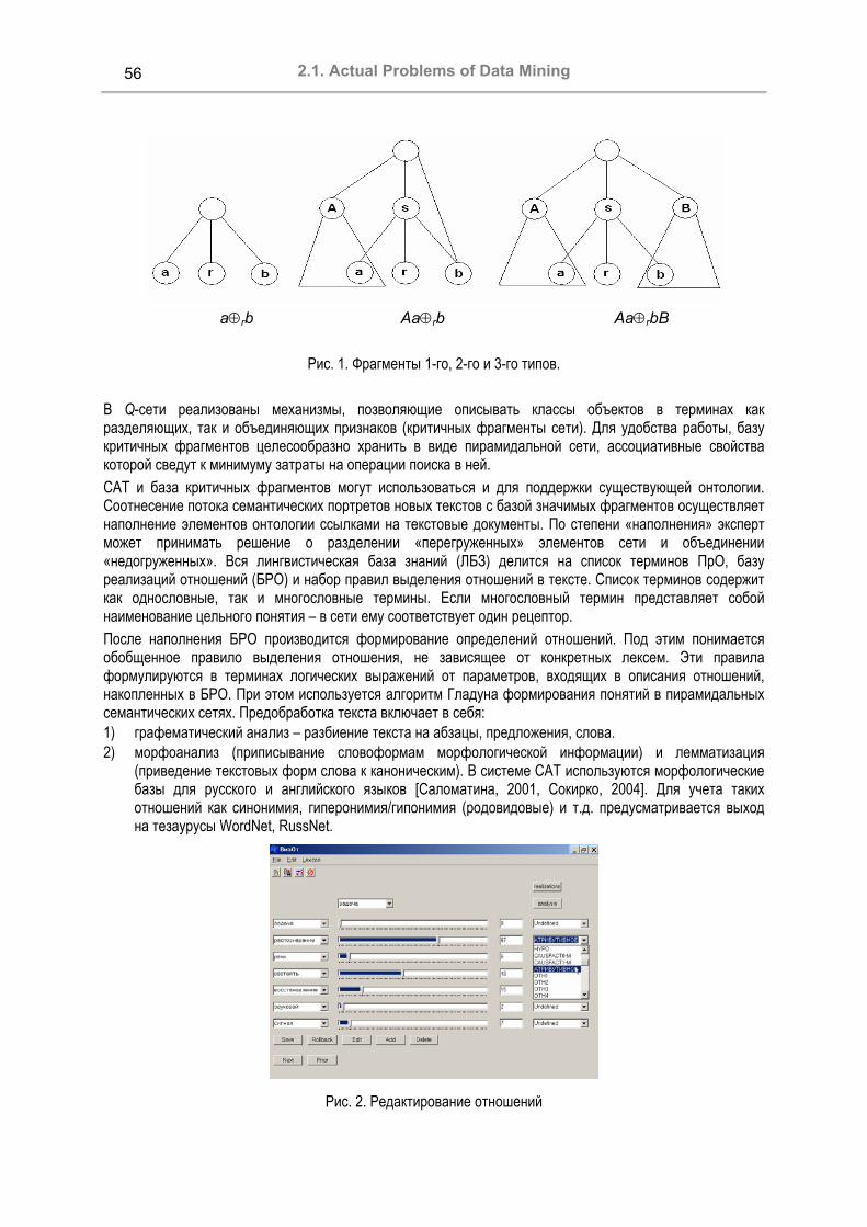
2.1. Actual Problems of Data Mining
56
a⊕rb Aa⊕rb Aa⊕rbB
Рис. 1. Фрагменты 1-го, 2-го и 3-го типов.
В Q-сети реализованы механизмы, позволяющие описывать классы объектов в терминах как разделяющих, так и объединяющих признаков (критичных фрагменты сети). Для удобства работы, базу критичных фрагментов целесообразно хранить в виде пирамидальной сети, ассоциативные свойства которой сведут к минимуму затраты на операции поиска в ней. САТ и база критичных фрагментов могут использоваться и для поддержки существующей онтологии. Соотнесение потока семантических портретов новых текстов с базой значимых фрагментов осуществляет наполнение элементов онтологии ссылками на текстовые документы. По степени «наполнения» эксперт может принимать решение о разделении «перегруженных» элементов сети и объединении «недогруженных». Вся лингвистическая база знаний (ЛБЗ) делится на список терминов ПрО, базу реализаций отношений (БРО) и набор правил выделения отношений в тексте. Список терминов содержит как однословные, так и многословные термины. Если многословный термин представляет собой наименование цельного понятия – в сети ему соответствует один рецептор. После наполнения БРО производится формирование определений отношений. Под этим понимается обобщенное правило выделения отношения, не зависящее от конкретных лексем. Эти правила формулируются в терминах логических выражений от параметров, входящих в описания отношений, накопленных в БРО. При этом используется алгоритм Гладуна формирования понятий в пирамидальных семантических сетях. Предобработка текста включает в себя: 1) графематический анализ – разбиение текста на абзацы, предложения, слова. 2) морфоанализ (приписывание словоформам морфологической информации) и лемматизация
(приведение текстовых форм слова к каноническим). В системе САТ используются морфологические базы для русского и английского языков [Саломатина, 2001, Сокирко, 2004]. Для учета таких отношений как синонимия, гиперонимия/гипонимия (родовидовые) и т.д. предусматривается выход на тезаурусы WordNet, RussNet.
Рис. 2. Редактирование отношений

KDS 2005 Section 2: Data Mining and Knowledge Discovery
57
Для автоматизации построения базы реализаций семантических отношений, а также для построения Q-сетей по текстам нами разработана программа «Визуализатор отношений» (ВизОт), ориентированная на поддержку работы эксперта [Загоруйко,1999]. При загрузке текста, ВизОт проводит его нормализацию и предоставляет эксперту набор обнаруженных в тексте лексем. В верхнем окне на экране дисплея (см. рис. 2) эксперту предъявляется некоторая лексема s0, а в серии окон слева показывается ряд других лексем s1, s2,…, si,…, sn. Эксперт может указать, какому отношению соответствует сочетание двух лексем (s0, si), и с какой вероятностью эти две лексемы, встретившись совместно в тексте данной ПрО, реализуют данное отношение. Вероятность ρ(s0, si) указывается положением курсора на отрезке 0-100 и числовым значением (%) в окнах центральной части экрана, а имя отношения выбирается из списка в правом окне на той же строке, где стоит лексема si. В ВизОт реализован алгоритм семантического анализ текста с использованием БРО и построение Q-сети текста по результатам этого анализа.
Автоматизации процессов создания и развития онтологии в GRID-сети
Структура системы автоматизированного построения онтологий «OntoGRID» должна отражать специфику трех типов ее клиентов: Эксперт, Пользователь и Администратор [Завертайлов,2004]. С точки зрения представления, создаваемая онтология - это комплект документов определённой структуры. Процесс построения онтологии состоит из итераций по дополнению и изменению этого комплекта документов. По результатам проведения ряда итераций администратор принимает решение о завершении очередного этапа процесса построения онтологии и публикации ее очередной стабильной версии. Система, поддерживающая автоматизированное создание и обработку документов онтологии в распределенном режиме, характеризуется набором специфических требований, определяющих ее технологическую организацию. Эти требования определяются тем, что в создании онтологии участвуют многочисленные географически разделенные коллективы экспертов. Топология задействованных узлов сети разработчиков меняется по мере подключения новых коллективов или прекращения работы старых. Адекватную основу для построения систем, удовлетворяющих таким требованиям, предоставляют вычислительные технологии, известные под общим названием GRID [GRID,2003]. Из них наиболее развитый инструментарий предлагается консорциумом The Globus Alliance. К числу последних разработок этого консорциума относится архитектура OGSA (Open Grid Services Architecture), основанная на концепции веб-сервисов. При разработке представления структуры онтологии были рассмотрены различные существующие на сегодняшний день подходы и стандарты. Как наиболее обоснованный и перспективный был принят стандарт OWL (Ontology Web Language) [Smith,2004], разработанный и рекомендованный консорциумом W3C. OWL обладает большей выразительной силой, чем такие структурные языки как XML, RDF и RDF-S, и может быть представлен в их форме. OWL-документ позволяет, используя лежащую в основе OWL дескриптивную логику, выводить такие факты о сущностях предметной области, которые не содержатся непосредственно в этом документе. В нашем проекте используется представление онтологии в нотации OWL-RDF. Для упрощения разработки новых онтологий удобно создавать шаблоны онтологий различных групп предметных областей. Данный проект ориентирован на построение шаблона онтологий научно-технических предметных областей, связанных с процессами анализа, синтеза и преобразования информации о произвольных фрагментах реального мира. К числу таких процессов относятся измерение и накопление данных, обнаружение закономерностей (знаний), хранение, обработка и передача данных и знаний, использование знаний для прогнозирования и синтеза [Galunov, 2004]. На рис. 3 приведен перечень базовых категорий онтологий проблемных областей такого рода. В дополнение к основному содержанию онтологии возможно формирование и хранение метаинформации об её элементах. Содержание метаинформации определяется в соответствии со стандартами Dublin (Guidelines for Implementing Dublin Core in XML) [Powell,2003], которые обеспечивают элементы онтологии такими данными, как реквизиты автора и соавторов, время создания и публикации, источники информации и т.д.

2.1. Actual Problems of Data Mining
58
В качестве индивидуального средства работы эксперта с фрагментом онтологии планируется использовать редактор, разработанный группой Protege Project [Protégé,2003]. Это средство обеспечивает удобный визуальный контроль за процессом разработки фрагментов онтологии. Описанная структура представления информации и архитектура ключевых сервисов были успешно апpобиpованы в ходе создания прототипа. В настоящее время ведутся работы по дальнейшей реализации системы OntoGRID.
структура использование использование решения
использование реализация
Рис. 3. Базовые категории онтологии
Заключение
Параллельно с описанными выше исследованиями по созданию инструментальной системы OntoGRID ведется подготовительная работа по организации виртуального коллектива экспертов из различных исследовательских центров, занимающихся проблемой «Интеллектуальный Анализ Данных» (Data Mining) для совместной разработки онтологии этой предметной области. С этой целью создается общедоступный двуязычный сайт, на котором будут помещены описания концепции и первого варианта предлагаемой онтологии. В настоящее время такой сайт (на русском и английском языках) создается на сервере Института Математики СО РАН. Авторы выражают благодарность Борисовой И.А., Дюбанову В.В., Кутненко О.А., Соколовой А.П. и Чуриковой В.А. за активное и полезное участие в обсуждении вопросов, затронутых в этой статье.
Библиография
[Ontology] http://xml.com/2002/11/06/Ontology_Editor_Survey.html [Dean,1070] Dean S. Worth, Andrew S. Kozak, Donald B. Johnson. Russian Derivational Dictionary. American Elsevier
Publishing Company, Inc. New York, 1970. [Гусев,1083] Гусев В.Д. Механизмы обнаружения структурных закономерностей в символьных последовательностях
// Проблемы обработки информации. – Новосибирск, 1983. – Вып. 100: Вычислительные системы. – С. 47 – 66. [Белоногов,2002] Белоногов Г.Г., Быстров И.И., Новоселов А.П. и др. Автоматический концептуальный анализ
текстов // НТИ, сер. 2. – 10, 2002. – С. 26 – 32.
Предметная область
“категория” наблюдаемые
объекты
“категория” наблюдаемые
свойства
“категория” типы задач
“категория” примеры решаемых задач
“категория” знания и гипотезы
“категория” методы
решаемых задач
<< структура >>

KDS 2005 Section 2: Data Mining and Knowledge Discovery
59
[Гусев,2004] Гусев В.Д., Саломатина Н.В. Алгоритм выявления устойчивых словосочетаний с учетом их вариативности (морфологической и комбинаторной) // Труды международной конференции Диалог – 2004 "Компьютерная лингвистика и интеллектуальные технологии", Верхневолжский, 2 – 7 июня 2004. – М., Наука, С. 530 – 535.
[Пащенко,1983] Пащенко Н.А., Кнорина Л.В., Молчанова Т.В. и др. Проблемы автоматизации индексирования и реферирования // Итоги науки и техники. Информатика – Т. 7, 1983. – С. 7 – 165.
[Гусев,2002] Гусев В.Д., Немытикова Л.А., Саломатина Н.В. Выявление аномалий в распределении слов или связных цепочек символов по длине текста // Интеллектуальный анализ данных. – Новосибирск, 2002. – Вып. 171: Вычислительные системы. – С. 51 – 74.
[Гладун,1987] Гладун В.П. Планирование решений. Киев. Наукова думка, 1987. С.17-51. [Кузнецов,1986] Кузнецов И.П. Семантические представления. Изд. «Наука», М. 1986 г. [Загоруйко,2004] Загоруйко Н.Г., Налетов А.М., Соколова А.А., Чурикова В.А.. Формирование базы лексических
функций и других отношений для онтологии предметной области //Труды конференции Диалог-2004. С.202-204. [Саломатина,2001] Саломатина Н.В. Количественные характеристики вариативности морфемных моделей (на
материале словаря канонических форм русского языка) // Методы обнаружения эмпирических закономерностей . – Новосибирск, 2001. – Вып.167: Вычислительные системы. – С. 93 – 114.
[Сокирко,2004] Сокирко А.В. Морфологические модули на сайте www.aot.ru //Труды конференции Диалог-2004. С.559-564.
[Загоруйко,1999] Загоруйко Н.Г. Метрологические свойства эксперта.// Обнаружение эмпирических закономерностей: Вычислительные системы, вып. 166, Тр. ИМ СО РАН, Новосибирск, 1999. С.119-128.
[Завертайлов,2004] Завертайлов А.В., Ковалев С.П. Система поддержки деятельности распределенных экспертных групп по разработке онтологий предметных областей // Труды Международной конференции по вычислительной математике <МКВМ-2004>. Рабочие совещания. Новосибирск: ИВМиМГ СО РАН, июнь 2004. С. 56-65.
[GRID,2003] Grid Computing: Making the Global Infrastructure a Reality. N. Y.: Wiley & Sons, 2003. [Smith,2004] Smith M.K., Welty C., McGuinness D.L. OWL Guide. W3 Consortium, 2004. http://www.w3.org/TR/owl-guide/. [Galunov, 2004] Valery I. Galunov, Boris M. Lobanov and Nikolay G. Zagoruiko. Ontology of the subject domain “Speech
signals recognition and synthesis”// Proc. of 9-th International Conference “Speech and Computer” (SPEECOM’2004), Saint-Peresburg, September 2004, p.448-454.
[Powell,2003] Powell A., Johnston P. Guidelines for implementing Dublin Core in XML. DCMI, 2003. http://dublincore.org/documents/dc-xml-guidelines/.
[Protégé,2003] Protege Project. http://protege.stanford.edu.
Информация об авторах
Николай Г. Загоруйко – Институт Математики СО РАН, пр. Коптюга, 4, Новосибирск, 630090, Россия; e-mail: [email protected] Владимир Д. Гусев – Институт Математики СО РАН, пр. Коптюга, 4, Новосибирск, 630090, Россия; e-mail: [email protected] Александр В. Завертайлов – Новосибирский Государственный Университет, ул. Пирогова, 2, 630090, Россия; e-mail: [email protected] Сергей П. Ковалёв – Новосибирский Государственный Университет, ул. Пирогова, 2, 630090, Россия; e-mail: [email protected] Андрей М. Налётов – Институт Математики СО РАН, пр. Коптюга, 4, Новосибирск, 630090, Россия; e-mail: [email protected] Наталия В. Саломатина – Институт Математики СО РАН, пр. Коптюга, 4,Новосибирск, 630090, Россия; e-mail: [email protected]

2.1. Actual Problems of Data Mining
60
APPLICATION OF THE MULTIVARIATE PREDICTION METHOD TO TIME SERIES 1
Tatyana Stupina, Gennady Lbov Abstract: An approach to solving the problem of heterogeneous multivariate time series analysis with respect to the sample size is considered in this paper. The criterion of prediction multivariate heterogeneous variable is used in this approach. For the fixed complexities of probability distribution and logical decision function class the properties of this criterion are presented.
Keywords: the prediction of multivariate heterogeneous variable, multivariate time series, the complexity of distribution.
Introduction
Let certain object (process) is described by the set of random features n1 XXX ,...,= , changing on time. On the base of analysis information, that presents features measurements in the consequent moments time series (prehistory), it is necessary to predict a values of features set m1 YYY ,...,= at certain future time moment (in particular, XY ⊆ . Distinguishing feature of considered below prediction problems is the measured features heterogeneity: the variable set be able consist of binary, nominal and quantitative variables simultaneously. In this case, multivariate time series presents itself a set of binary, symbol and numeric random sequences. Classical methods are directed to the analysis of numeric sequences basically. Many methods allow analyse univariate binary or symbol sequences. However the most of important applied problems number are concerned with need to heterogeneous time series analyse. There is reason to suppose in some problems that time series is the realization of random processes, in which probabilistic characteristics (distribution) are saved on a time. At other times such suggestions to do it is impossible under the matter of problem (probabilistic characteristics of process are changed on time). There is possible to offer a different depending on specified suggestions targets setting and the different methods of their decision accordingly. The methods of heterogeneous time series analysis for different targets setting, including the logical deciding functions class for heterogeneous variable are considered in work [Lbov G.S., 1994].
The Target Setting
One is considered the n – measured heterogeneity random process )(),...,(),...,( tXtXtXG nj1= . Let it set of predictable characteristic is jj XY = , n1j ,...,= . Fix some consequent moments of the time, NR1 ≤≤ .
Denote the value random variable jX at a moment of the time dt , jX
dj Dx ∈ , as this d
jx , and dx is the value
random variable of X , Xd Dx ∈ , ∏
==
n
1jXX j
DD . The problem consist of that, it is necessary to predict the values
set ),...,,...,( nj1 yyyy = at certain future moment of the time 1Rt + , where 1Rjj xy += using the data,
characterizing prehistory, djxb = , n1j ,..,= , R1d ,...,= . It is necessary to build decision function, allowing
predict a set of values ),...,,...,( nj1 yyyy = on prehistory b.
The set of every possible all prehistory, that have line measure R denote as B , and the set of every possible all
sets y denote as YD , Bb ∈ , YDy ∈ , ∏=
=n
1jYY j
DD . Let us understand a prediction decision function as a f
mapping of the B set on the YD set, i.e. YDBf →: . At the building decision functions f is used following
1 This work was financially supported by RFBR-04-01-00858

KDS 2005 Section 2: Data Mining and Knowledge Discovery
61
hypothesis: It is supposed that conditional distribution )/( byP does not depend on the shift on the time, i.e. distribution is specified for moments of the time 1RR1 ttt +,,..., is contemporized with distribution for moments of the time TtTtTt 1RR1 ∆±∆±∆± +,,..., . If the conditional distribution )/( byP is known, then it is possible to find optimum prediction decision function of . Since specified distribution is unknown, decision function shall be constructed on the base of multivariate time series analysis. Let the features nj1 XXX ,...,,..., are measured at consequent moments of the time with the gap 1dd ttt −−=∆ for the random process G . Denote this set of moments as ,...,,..., Nk1 tttT = . Thus, the empirical information is presented by n – measured heterogeneity time series N1kn1jxq k
j ,...,,,...,, === . The set of values
),...,,...,( dkn
dkj
dk1
dk xxxx −−−− = will is called prehistory with the number d , correlated with a moment of the time
kt , N1Rk ,...,+= . The prehistory with line measure R for a specified moment of the time kt is denoted as a table dkk xb −= , R1d ,...,= . Note that univariate symbol sequence for 1R = is the realization of simple Markoff process with the transfer probability matrix )/( xyP , Ax ∈ , Ay ∈ , A –an alphabet of symbols. Decision function f , constructed on the base of set prehistory analysis with line measure R, is named sample decision function of prediction. It is necessary to construct the sample decision function on the small sample in the multivariate heterogeneous space, so the most proper class is a class of logical decision functions [Lbov G.S., Starceva N.G, 1999]. Methods of time series analysis propose to decision of problem in two stages: It is constructing decision function for fixed prehistory with the number d ( R1d ,...,= ) it is constructing the generalise logical decision function (mapping
YDBf →: ). The first stage is consist of decision the prediction multivariate variable problem Y on other multivariate variable X, i. е. for each prehistory d we have two data tables dkx − , ky , N1Rk ,...,+= , on base which necessary to construct the sample decision function (mapping YX DD → ). Below it is considered a decision of this problem, in which is used criterion, introduced in work [Lbov G.S., Stupina T.A., 2002].
The Performance Criterion of Prediction
In the probabilistic statement of the problem, the value (x,y) is a realization of a multidimensional random variable (X,Y) on a probability space >ΡΒΩ< ,, , where YX DD ×=Ω is µ -measurable set (by Lebeg), Β is the borel σ -algebra of subsets of Ω , Ρ is the probability measure (probability distribution) on Β , XD is heterogeneous domain of under review variable, nDx =dim , yD is heterogeneous domain of objective variable, mDy =dim .
Definition 1. The strategy of nature is c=p(x,y)=p(x)p(y/x)), where a conditional probability p(y/x) is specified for any elements on Β . Let us put oΦ is a given class of decision functions. Class oΦ is µ -measurable functions that puts some subset of the objective variable Yy DE ⊆ to each value of the under review variable XDx ∈ , i.e. : yD
x 2Df →=Φo . This class of decision function is more total than class of logical decision functions [Lbov G.S., Starceva N.G, 1999]. In this paper, we will consider criterion for decision function from total class oΦ . So criterion was considered for logical decision functions in work [Lbov G.S., Stupina T.A., 2002]. But here we will achieve that class of logical decision functions is a universal class about relative to criterion. The quality ),( fcF of a decision function oΦ∈f under a fixed strategy of nature c is determined as follows.
)()))(()/)(((),( xdPxEµxxEPfcF yD
yx
−= ∫ ,
where )()( xfxEy = is a value of decision functions in x, )/)(( xxEyP y∈ is a conditional probability of event yEy ∈ under a fixed x, ))(( xEµ y is measurable of subset yE . Note that if ))(( xEµ y is probability measure,

2.1. Actual Problems of Data Mining
62
than criterion ),( fcF is distance apart distributions. If the specified probability coincides with equal distribution than such prediction does not give no information on predicted variable (entropy is maximum). The measure
))(( xEµ y = ∏=
=m
1j y
y
Y
y
j
j
DµEµ
DµEµ
)(
)(
)()(
is the normalized measure of the subset yE and it is introduced with taking into
account the type of the variable. The measure ))(( xEµ y is measure of interval, if we have a variable with ordered set of values and it is quantum of set, if we have a nominal variable (it is variable with finite non-ordering set of values). Clearly, the prediction quality is higher for those yE whose measure is smaller (accuracy is higher) and the conditional probability )/)(( xxEyP y∈ (certainty) is larger.
For a fixed strategy of nature c, we define an optimal decision function )(xfo as function for which ),(sup),( fcFfcF f oo Φ∈= , where oΦ is represented above class of decision functions.
As a rule, the strategy of nature is unknown; for this reason, a decision function is constructed from a training sample N1i
ii yxv ,...,),( == by sampling criterion )(fF with the use of some algorithm fvQ =)( , where )(xf is a sampling decision function and N is the size of the training sample. The sampling criterion )(fF is empirical risk of the criterion ),( fcF . When we solve this problem in practice the size of sample is very smaller and type of variables different. In this case is used class of logical decision function. The logical decision function f is assigned the pair >< βα, , where Mα Ψ∈ and MRβ∈ . The class MΨ is the set of partitions ,...,,..., M
xtx
1x EEEα = of the space XD into
disjoint subsets for which ∏=
=n
1i
tx
tx i
EE , ii X
tx DE ⊆ , ∅≠t
xiE and
ii Xtx WE ∈ , where
iXW is the set of all possible
intervals if iX is a variable with ordered set of values and iXW is the set of arbitrary subsets of
iXD if iX is a
nominal variable, i.e. a variable with a finite unordered set of values; we have Xtx WE ∈ , where ∏
==
n
1iXX i
WW .
The class MR is the set of decisions (arbitrary subset of the space YD ) ,...,,..., My
ty
1y EEEβ = for which
∏=
=m
1i
ty
ty i
EE ,ii Y
ty DE ⊆ , ∅≠t
y iE and ∅≠t
y iE , where
iYW is defined so as iXW . The decision function is
presented in simple form for understanding: if txEx ∈ than t
yEy ∈ . The subsets txE and t
yE represented as above can be described in terms of conjunctions of simple predicates. Such a coarsening of the decision function is caused by the necessity to construct solutions from small samples. The class of logical decision function MΦ can be represented as MM R×Ψ . Under the assumptions made, the complexity of the class MΦ is only determined by the M parameter:
Mν M =Φ )( . Thus, the larger the number M, the more complex the class MΦ . We achieve important property of this class by theorem. Theorem. For a fixed type of the predicate, the class MΦ of logic decision functions is a universal class in the problem of prediction multivariate heterogeneous value by criterion F(c,f), i.e. for any strategy of nature c and any
0ε > there exists a number M (M=1,2,3,…) and for some logical decision function f MΦ∈ (it is represented in the form of decision tree on M vertices) such that εfcFfcF ≤− ),(),( o , where of is optimal function in class oΦ . The proof of this theorem readily follows from the property of µ -measurability and P-measurability of space D and its projections on the space XD , YD correspondingly. The proof for the case where Y is a discrete variable is given in [Lbov G.S., Starceva N.G, 1994]. The proof for the case where Y is a continuous variable is given in [Berikov V.,1995].
KDS 2005 Section 2: Data Mining and Knowledge Discovery
63
We can introduce a complexity of distribution (strategy of nature c) using the class logical decision function. It is necessary for solving statistical stability problem of decision function. Statement 1. For any nature strategy c the quality criterion ),( fcF (risk function) of logical decision function f belonging to MΦ is presented by following expression:
∫ ∫ −=X YD D
dxdyyxpxfyL1fcF ),()))(,((),( ∑=
−=M
1t
ttxy
tx µpp )( / ,
where the loss function ),( fyL such as ⎩⎨⎧
∉∈
+=
βyβy
p1p
fyLo
o ,),( , )( tYo Eµp = , Mααfβ Ψ∈= ),( .
Proof.
)()))(()/)(((),( xdPxEµxxEPfcF yD
yx
−= ∫ = ∑ ∫ ∫ ∫= ⎥
⎥⎦
⎤
⎢⎢⎣
⎡−
M
1t E E Eo
tX
tY
tX
dxxppdxdyyxp )(),( =
∑ ∫ ∫ ∫ ∫= ⎥
⎥⎦
⎤
⎢⎢⎣
⎡−+
M
1t E E E Do
tX
tY
tX Y
dxdyyxppdxdyyxp ),()(),( =
∑ ∫ ∫ ∫ ∫ ∫ ∫= ⎥
⎥⎦
⎤
⎢⎢⎣
⎡−−−+−
M
1t E E E D E Eooo
tX
tY
tX Y
tX
tY
dxdyyxppdxdyyxppdxdyyxpp1 ),()(),()(),()( =
∑ ∫ ∫∫= ⎥
⎥⎦
⎤
⎢⎢⎣
⎡−+−=
M
1t E Eo
Eo
tX
tY
tY
dxdyyxppdxdyyxpp1 ),()(),()( ∫ ∫ −=X YD D
dxdyyxpxfyL1 ),()))(,(( .
Definition 2. To each subclass MΦ we put in correspondence the subset )(MLε = ),(),(,: εfcFfcFfc M ≤−Φ∈∃ o of nature strategies; ε is an arbitrarily small number determining an
admissible error level of this subset of strategies, where of is optimal function in class oΦ . The complexity measure of each subset )(MLε is defined as the complexity measure of the corresponding subclass of decision functions: MνMLν Mε =Φ= )())(( . Accordingly, the nature strategy c belonging to )(MLε has complexity measure M. The important statement follows from this theorem and definition. Statement 2. The set of all possible strategies can be ordered according to complexity, i.e.
oLML2L1L εεε ⊂⊂⊂⊂⊂ ...)(...)()( , and M1M εε ≤+ , where ))(( MLν ε =M is the complexity and Mε is the admissible error level of the strategy class ))(( MLν ε . Proof. For an arbitrary M, let us prove the embedding )()( 1MLML εε +⊂ i.e. show that )(MLc ε∈∀ ,
1Mf +Φ∈∃ such that εfcFfcF ≤− ),(),( o . The definition of the class )(MLε implies that Mg Φ∈∃ such that MεfcFgcF ≤− ),(),( o . Since 1MM +Φ⊂Φ , we can obtain f from g by partitioning some subset t
XE into two subsets: if >< βαg ,~ , M1t
tXEα ,..., == , M1t
tYEβ ,..., == than >′′< βαf ,~ ,
/,...,,,..., 2121 tX
tX
tX
MX
tX
tX
1X EEEEEEEα ∪==′ , /,...,,,..., 2121 t
YtY
tY
MY
tY
tY
1Y EEEEEEEβ ∪==′ , where
)()()( 21 tX
tX
tX EµEµEµ += and )()()( 21 t
YtY
tY EµEµEµ +≥ .
Therefore, M1M εεεfcFfcF ≤=≤− +),(),( o , it is followed from the definition ),( fcF .
We can suppose that the true (optimal) decision function belongs to MΦ it is followed from this statement 1. Definition 3. Define a nature strategy Mc (generated by logical decision function Mf Φ∈ ) such as set of parameters satisfying the following conditions:
1) 1pM
1t
tx =∑
=,
2) txy
tX
tY pEEP /)/( = (conditional distribution is same for any t
XEx ∈ and tYEy ∈ ),

2.1. Actual Problems of Data Mining
64
3) txy
tX
tY p1EEP /)/( −= ,
where αE tX ∈ , βE t
Y ∈ , Mfβα Φ∈>< ~, . The complexity of this strategy is M, i.e. Mcν M =)( . Note that Mc generated by logical decision function belongs to class )(MLε . Clearly, the decision function that generated this strategy is optimal function in class MΦ .
Statement 3. For a fixed nature strategy )(MLc εM ∈ of complexity M the quality criterion )~
,( fcF M (risk function) of logical decision function Mf ′Φ∈
~ of complexity M ′ is presented in following form:
∑∑′
=′
′′′′
=′
′′ −===M
1t
ty
txy
tx
M
1t
ttxM µppρpαFfcF )~(~~)~()
~,( / ,
where ∑=
′′′ ∩
=∈=M
1ttX
tX
tXt
xtX
tx Eµ
EEµpExPp)(
)~
()~
(~ ,
⎟⎟⎠
⎞⎜⎜⎝
⎛
−∩−
−+∩∩
=′′′
=
′
′′ ∑ )(
)~
()~
()()(
)~
()(
)~
(~
~/// t
Y
tY
tY
tYt
xytY
tY
tYt
xy
M
1ttX
tX
tXt
xtx
txy Eµ1
EEµEµp1Eµ
EEµpEµ
EEµpp1p .
Proof. Since the decision function f~
belongs to class M′Φ than there exists partition ~
,...,~
,...,~
~ MX
tX
1X EEEα ′′=
of space XD and according to it the set of subsets ~
,...,~
,...,~
~ M
YtY
tY EEEβ ′′′= of space YD . The expression of
the criterion ∑′
=′
′′′ −=M
1t
ty
txy
tx µppfcF )~(~)
~,( / follows from statement 1, where )
~(~ t
Xtx ExPp ′′ ∈= ,
)~
/~
(~/
tX
tY
txy ExEyPp ′′′ ∈∈= . Since the strategy Mcc = , )(MLc εM ∈ is generated by logical decision function
Mβαf Φ>∈< ,~ , there is a partition ,...,,..., MX
tX
1X EEEα = of space YD and according to it the set of
subsets ,...,,..., MY
tY
1Y EEEβ = of space YD , the sets of parameters )( t
Xtx EPp = , )/(/
tX
tY
txy EEPp = as
provided by definition 3. Late for simplicity we will not write the mark ‘∈’ and ‘ ∩ ’ in view of the events. Express the t
xp ′~ and txyp ′
/~ by way of t
xp and txyp / take account of the event distribution is inside of subsets t
XE , tYE :
∑=
′′′′ =∪==M
1t
tX
tX
tX
tX
tX
tX
tx EEPEPEEPEPp )/
~()()
~()
~(~ = ∑
=
′M
1ttX
tX
tXt
x EµEEµp
)()
~( ;
)~~
(~)~
()
~~()
~/
~(~
/tX
tYt
xtX
tX
tYt
Xt
Yt
xy EEPp1
EPEEPEEPp ′′
′′
′′′′′ === ,
∑=
′′′′′′′′ ==∪==M
1t
tX
tYY
tX
tX
tYY
tX
tX
tY
tX
tY EEDEPEEDEPEEDPEEP )
~~()
~~()
~~()
~~( ))
~~()
~~(( t
XtY
tY
tX
M
1t
tX
tY
tY
tX EEEEPEEEEP ′′
=
′′ +∑ ,
,)(
)~
()(
)~
(
)())
~~()(()/
~~()()
~~(
/ tY
tY
tYt
xytX
tX
tXt
x
tY
tX
tY
tX
tY
tXt
xytY
tX
tY
tX
tY
tX
tX
tY
tY
tX
EµEEµp
EµEEµp
EEµEEEEµpEEEEPEEPEEEEP
′′
′′′′′′
=
=∩
==
,)(
)~
()()(
)~
()(
))~~
()(()(
)/~~
()()~~
(
// tY
tY
tYt
xytX
tX
tXt
xtY
tX
tY
tX
tY
tXt
xytx
tY
tX
tY
tX
tY
tX
tX
tY
tY
tX
EµEEµp1
EµEEµp
EEµEEEEµp1p
EEEEPEEPEEEEP′′′′
′′′′
−=∩
−=
==
where )(
)~
()~
()(
)~
(tY
tY
tY
tY
tY
tY
tY
Eµ1EEµEµ
EµEEµ
−−
=′′
and tYY
tY EDE \= .

KDS 2005 Section 2: Data Mining and Knowledge Discovery
65
Remark. If the nature strategy Mc such that some subset tYE coincides with the space YD , than
)()
~(
)()
~(
~~
// tY
tY
tYt
xy
M
1ttX
tX
tXt
xtx
txy Eµ
EEµpEµ
EEµpp1p ∩∩
=′
=
′
′′ ∑ .
It is followed from that 1EDPp tXY
txy == )/(/ , 1Dµ Y =)( .
Consequence 1. If the decision function f~ belonging to MΦ coincides with the function f belonging to MΦ ,
than ),()~
,( fcFfcF = .
Consequence 2. For the decision function f~ belonging to M′Φ we have the expression t
xytX
tY p1EEP ′′′ −= /
~)~
/~
( . Really, it is follows from the statement 3, where
)E()E~E()E(
)E()EE~(
tY
tY
tY
tY
tY
tY
tY
µµµ
µµ ′′ −
= , )E(
)E~E()E~()E()E(
)EE~(tY
tY
tY
tY
tY
tY
tY
tY
µ1µµµ1
µµ
−
+−−=
′′′
.
Consequence 3. If we have M = 1 and the optimal function f generating 1c such that Y1Y DE = ,
than 0fcF 1 =),( .
Really, for the express of criterion we have ( )∑=
=−=−=M
1tYoYXo
tYo
tY
tX 0DPDDPEPEEPfcF )()()()(),( .
It means that we have the event distribution in D for the nature strategy of the complexity M=1. It is case when the entropy is maximum. Consequence 4. If we have M = 1 and the optimal function f generating 1c such that Y
1Y DE = ,
than for any decision function Mf ′Φ∈~ the criterion 0fcF 1 =)
~,( .
Really, )E~()D/D(P)D(
)DE~(p~ tYXYo
Y
YtYt
x/y′
′′ == µ
µµ , )
~()(
)()
~(~ t
XXoX
Xt
Ytx EµDP
DµDEµp ′
′′ == ,
∑′
=′
′′′ =−=M
1t
tY
tY
tX1 0EµEµEµfcF .))
~()
~()(
~()
~,(
Consequence 5. If the decision function f~ belongs to 1Φ and Y
1Y DE =
~ , than we have 0fcF M =)~
,( for any complexity 1M ≥ .
Really, we have ∑=
==M
1ttX
tXXt
xx 1Eµ
EDµpp)(
)(~ , 1Eµ1
EDµ1p1Eµ
EDµpppM
1ttY
tYYt
xytY
tYYt
xytxxy =⎟⎟
⎠
⎞⎜⎜⎝
⎛
−−
−+= ∑= )(
)()()(
)(~/// .
As stated above when the nature strategy is unknown the problem of statistical stability of sample decision functions is appeared. The quality ),( fcF of sample decision function depends on the size N of the sample, the complexity M of the distributions, and the complexity M ′ of the class of functions M ′Φ used by the algorithm
)(vQ and empirical criterion )(fF for constructing sample decision functions f . The empirical criterion )(fF (empirical risk function) is presented by expression:
∑=
=−=N
1i
ii yxL1N1fF )),(()( ∑∑
=
′
=−=⎟
⎟⎠
⎞⎜⎜⎝
⎛−
M
1t
ttxy
tx
ttX
tX
tY
M
1t
tX µppµ
ENEEN
NEN )ˆˆ(ˆ
)~
()
~~()
~(
/ ,
where )(∗N is a number of sample spots belonging to the corresponding subset *, )~
(ˆ tY
t Eµµ = , >< βαf
~,~~ M′Φ∈ .
On the one hand, if the constraints on the class of decision functions are too strong, then this class may be inadequate to the true distribution, and the higher the degree of inadequacy, then poorer the quality of the decision function. On the other hand, using a complex class of functions on small samples also lowers the quality for the decision function.

2.1. Actual Problems of Data Mining
66
At present time there are two well-known approaches solving this problem. The Vapnik -Chervonenkis approach uses the principle of uniform convergence [Vapnik V.N., Chervonenkis A.Ya, 1970]: the quality criterion
),( fcF depends on VC-complexity of the decision function class Φ and the level of empirical risk )(fF . In the case of one discrete variable prediction was provided results [Nedelko V.M., 2004]. When the nature strategy c belongs to even probability distribution class such problem was decided by the method of statistical modelling for the case of several heterogeneous variable prediction [Lbov G.S., Stupina T.A., 2003]. It is the particular case of our problem. Really, we can provide the biased estimator of criterion (risk function)
)(),( fFfcFEεENvN −= by the statistical modelling method for any nature strategy c belonging to the class
)(ML . It is follows from the consequence 1-4 that we have the expression )(fFEεENvN = for )(1Lc ∈ .
Another (Bayesian) approach to solving this problem consists in the construction of the evaluation ),( fcEF that is obtained by averaging over all samples of N-size. Raudys in [Raudis Sh.Yu.,1976] used that (Bayesian) approach to solving pattern recognition problem that is admitted small samples, but is imposed a fairly strong constraint on the form of the distribution. When the nature strategy is unknown, the quality of decision function is assigned by the expectation ),( fcEFEc of criterion ),( fcEF , which is obtained by averaging over all distributions. This problem was solved for pattern recognition problem in the case of one discrete variable prediction [Startseva N.G.,1995], [Berikov V.B., 2002] and for regression analysis in the case of one real variable prediction [Lbov G.S., Stupina T.A., 1999]. The problem concerned at this paper generalizes the problem of pattern recognition and the problem regression analysis. From the presented above properties of the quality criterion is followed that we can use both approaches solving statistical stability problem.
Conclusion
An approach to solving the problem of heterogeneous multivariate time series analysis with respect to the sample size was considered in this paper. The solution of this problem was assigned by means of presented criterion. The universality of the logical decision function class with respect to presented criterion makes the possible to introduce a measure of distribution complexity and order all possible distributions (nature strategies) according to this measure. The logical decision function class allows us to introduce such orderings in the space of heterogeneous multivariate variables. For the fixed complexities of probability distribution and logical decision function class, the properties of this criterion are presented by means of theorem, statements and consequences. The approaches to the solution of the statistical stability sampling decision function problem were considered.
Bibliography
[Lbov G.S., 1994] Lbov G.S. Method of multivariate heterogeneous time series analysis in the class of logical decision function. Proc. RBS, 339, Vol. 6, pp.750-753.
[Lbov G.S., Starceva N.G, 1999] Lbov G.S., Starceva N.G. Logical Decision Functions and Questions of Statistical Stability. Inst. Of Mathematics, Novosibirsk.
[Lbov G.S., Stupina T.A., 2002] Lbov G.S., Stupina T.A. Performance criterion of prediction multivariate decision function. Proc. of international conference "Artificial Intelligence", Alushta, pp.172-179.
[Lbov G.S., Starceva N.G, 1994] Lbov G.S., Starceva N.G. Complexity of Distributions in Classification Problems. Proc. RAS, Vol 338, No 5,pp 592-594.
[Berikov V.,1995] Berikov V. On the convergence of logical decision functions to optimal decision functions. Pattern Recognition and Image Analysis. Vol 5, No 1, pp.1-6.
[Vapnik V.N., Chervonenkis A.Ya, 1970] Vapnik V.N., Chervonenkis A.Ya .Theory of Pattern Recognition, Moscow: Nauka. [Nedelko V.M.,2004] Nedelko V.M. Misclassification probability estimations for linear decision functions. Proceedings of the
seventh International Conference "Computer Data Analysis and Modelling". BSU. Minsk. 2004. Vol 1. pp. 171–174. [Lbov G.S., Stupina T.A., 2003] Lbov G.S., Stupina T.A. To statistical stability question of sampling decision function of
prediction multivariate variable. Proc. of the seven international conference PRIP'2003, Minsk, Vol. 2, pp. 303-307.

KDS 2005 Section 2: Data Mining and Knowledge Discovery
67
[Raudis Sh.Yu.,1976] Raudis Sh.Yu. Limited Samples in Classification Problems, Statistical Problems of Control, Vilnus: Inst. Of Mathematics and Computer Science, 1976, vol. 18, pp. 1-185.
[Startseva N.G.,1995] Startseva N.G. Estimation of Convergence of the Expectation of the Classification Error Probability for Averaged Strategy, Proc. Ross. RAS, vol. 341, no. 5, pp. 606-609.
[Berikov V.B., 2002] Berikov V.B. An approach to the evaluation of the performance of a discrete classifier. Pattern Recognition Letters. Vol. 23 (1-3), 227-233
[Lbov G.S., Stupina T.A., 1999] Lbov G.S., Stupina T.A.. Some Questions of Stability of Sampling Decision Functions, Pattern Recognition and Image Analysis, Vol 9, 1999, pp.408-415.
Author's Information
Gennady Lbov – Institute of Mathematics SBRAS, 4 Koptuga St, Novosibirsk, 630090, Russia; e-mail: mailto:[email protected] Tatyana Stupina – Institute of Mathematics SBRAS, 4 Koptuga St, Novosibirsk, 630090, Russia; e-mail: mailto:[email protected]
К ОПРЕДЕЛЕНИЮ ИНТЕЛЛЕКТУАЛЬНОГО АНАЛИЗА ДАННЫХ
Ксения А. Найденова Аннотация: В работе рассматриваются ключевые проблемы интеллектуального анализа данных, анализируется содержание термина «интеллектуальный анализ данных (ИАД). Показывается роль методов машинного обучения для извлечения концептуальных знаний из данных. Рассматривается абстракция данных как метод формирования знаний. Взаимосвязь между базами данных и средствами машинного обучения выделяется как ключевая проблема реализации ИАД.
Ключевые слова: интеллектуальный анализ данных, машинное обучение, machine learning, извлечение знаний из данных, data mining.
Содержательный анализ ИАД
Несколько лет тому назад термин «интеллектуальный анализ данных» (ИАД) не был широко распространен, но широко употреблялся термин «интеллектуальные системы». Интеллектуальными назывались любые прикладные системы, независимо от их назначения, в которых для принятия решений в явном виде использовались знания специалистов, представленные в виде правил, процедур, эвристик, классификаций, моделей объектов и т. д. Использование знаний в интеллектуальных системах охватывало и охватывает не только проблемы извлечения знаний эксперта, но и всю проблематику машинного обучения (Machine Learning) с целью автоматизированного извлечения знаний из данных. Так, на 6-ой национальной конференции по искусственному интеллекту (КИИ-98) [Труды, 1998] работали следующие секции: «Прикладные системы», «Интеллектуальные системы и виртуальная реальность», «Интеллектуальные системы и формализация синтеза познавательных процедур», «Интеллектуальные производства и предприятия». Но уже через два года, на 7-ой национальной конференции по искусственному интеллекту (КИИ-2000) работала секция «Интеллектуальный анализ данных» [Труды, 2000]. Эта секция была посвящена работам в сравнительно новой области Data Mining (DM). Этот термин переводится как «добыча» полезных данных (сродни добыче полезных ископаемых) из баз данных (БД) и по существу употребляется как синоним термина «ИАД». Нередко наряду с Data Mining употребляются термины Knowledge Discovery (обнаружение знаний) и Data Warehouse (хранилище данных). ИАД и управление знаниями представляют сегодня самостоятельное направление в теории и приложении интеллектуальных систем [Забежайло, 1998а].

2.1. Actual Problems of Data Mining
68
ИАД выделяет подкласс задач, которые имеют дело с извлечением из данных зависимостей нестатистического характера. Такие зависимости позволяют делать заключения не в среднем по некоторому множеству объектов, а для каждого изучаемого объекта в отдельности. Исследуются объекты, описываемые не просто совокупностью элементов, но имеющие внутреннюю структуру, представленную набором качественных и количественных отношений между элементами. Практическая потребность в ИАД очень велика во всех областях, в том числе и в медицине, так как к настоящему времени в БД, поддерживающих различные системы принятия решений, накоплено такое количество информации, которое невозможно осмыслить и применить без помощи компьютера. Трудности анализа данных в больших хранилищах отягощаются не только объемом и разнородным характером данных, но и открытостью знаний специалиста и динамичностью практических потребностей. Какие именно знания необходимо получить специалисту из БД, невозможно сказать заранее, а тем более формализовать в виде стандартных запросов к БД. ИАД призван уменьшать все увеличивающийся разрыв между сбором данных и их пониманием. Практические цели ИАД: хранить данные, иметь к ним доступ в различных ситуациях, получать информацию для разных целей, часто не ограничиваясь форматом запросов к БД, создавать новые концепты и эффективно их использовать. Практические цели «извлечения знаний из данных» приводят к тому, что ИАД охватывает великое множество методов преобразования и анализа данных от первичной обработки данных до методов машинного обучения для выявления концептуальных знаний. Методы машинного обучения включают одновременно методы выявления логических правил (импликаций, причинных зависимостей) и методы аппроксимации различных зависимостей, которые не поддаются аналитическому описанию. ИАД охватывает также статистику, распознавание образов, нейронные сети, абстракцию данных (data abstraction), онтологии, средства визуализации для поддержки анализа данных и др. Трудно также разграничить ИАД и область, которая занимается построением БЗ на основе БД. ИАД и DM есть подзадачи одной общей задачи – Преобразование Данных в Знания. Разные авторы предъявляют различные, подчас противоречивые, требования к средствам анализа данных. По мнению ряда авторов, цель Data Mining состоит в выявлении скрытых закономерностей в больших и очень больших объемах данных, содержащих несколько миллионов и даже биллионов записей [Hand, 1998]. Разворачиваются дискуссии по поводу применимости статистических методов анализа данных в Data Mining. Традиционные методы статистики считаются основным инструментом анализа данных. Статистика оперирует усредненными характеристиками выборки, которые часто являются малоинформативными величинами при решении практических задач. Например, средняя платежеспособность клиента не позволяет прогнозировать состоятельность клиента и его намерения в условиях риска для принятия решений. Средняя интенсивность сигнала не выявляет характерных особенностей сигнала, положений пика сигнала и т. п. Вот взгляд на содержание термина «ИАД» российского выдающегося специалиста Н.Г. Загоруйко: «Методы интеллектуального анализа данных (Data Mining) применяются для автоматического обнаружения эмпирических закономерностей и использования их при решении задач классификации, распознавания образов и прогнозирования. Особенность этих методов состоит в их ориентации на задачи, для которых использование традиционных статистических методов вызывает значительные затруднения. Имеются в виду задачи анализа данных очень большого объема, плохо обусловленных таблиц (количество признаков сравнимо с количеством объектов), пораженных шумами и пробелами, с признаками, измеренными в разнотипных шкалах, при отсутствии оснований для выдвижения гипотез о законах распределения» [Загоруйко, 1999]. Можно заметить некоторые противоречия в требованиях к методам DM, например, традиционные статистические методы анализа данных не применимы к данным гигантского объема, являющимся конгломератом информации разнородного характера, поступившей от разных источников. Алгоритмы распознавания и машинного обучения в особенности имеют экспоненциальную сложность и плохо приспособлены, кроме специальных модификаций, к анализу данных гигантского объема. Тем не менее, они являются главным инструментом в DM. Обнаружение знаний в данных это область исследований, которая находится на пересечении технологии баз данных, статистики, машинного обучения (Machine Learning), распознавания образов, конструирования БЗ и многих других дисциплин, так или иначе связанных с обработкой данных и знаний.

KDS 2005 Section 2: Data Mining and Knowledge Discovery
69
Все авторы обзоров по ИАД [Загоруйко, 1999], [Забежайло, 1998б], [Рощупкина и Шапот, 1997], [Lavrač, 1998] согласны в том, что это направление связано с анализом гигантских объемов данных, накопленных в БД, с целью извлечения из них знаний в форме неожиданных, интересных, ранее неизвестных зависимостей, связей, ассоциаций, фактов. Большинство авторов согласны также и в том, какие методы обработки данных включаются в ИАД. Наиболее полный список методов представляется следующим образом:
1) первичная обработка данных (фильтрация, выделение однородных областей, анализ временных рядов, извлечение признаков и отдельных структурных элементов;
2) дискретизация данных (бинаризация, шкалирование, интервальный анализ, кластеризация, квантификация, укрупнение диапазонов и др.);
3) преобразование данных (быстрое преобразование Фурье, быстрое преобразование Уолша, преобразование пространства признаков и др.);
4) таксономия и методы выделения признаков; 5) выявление закономерных отношений статистическими (факторный анализ, корреляционный
анализ, регрессионный анализ) и логическими (Machine Learning) методами; 6) выявление информативных признаков; 7) методы анализа структурных объектов (динамическое программирование, скрытые марковские
процессы, иерархические структуры и др.); 8) распознавание образов и прогнозирование (нейронные сети; генетические алгоритмы,
моделирование правдоподобных рассуждений, заполнение пробелов в БД); 9) методы моделирования сложных объектов и систем; 10) нечеткие модели и мягкие вычисления.
Объединение в одном направлении такого большого количества различных методов требует объяснения. Но, что самое важное - цель ИАД не определена достаточно ясно. Какие именно знания извлекаются из данных, каждый исследователь понимает по-разному, исходя из задач своей специальной области. С точки зрения целей исследования главным является не объем данных, а природа данных, степень их генерализации, степень их структурированности (организованности) и степень их активности – то есть возможность их непосредственного использования, при решении задач. Таким образом, процесс извлечения знаний из данных при их анализе управляется содержанием тех знаний, которые пользователь хочет получить из данных. Чтобы более точно определить цели ИАД, рассмотрим, какие данные он объединяет. Это данные, которые имеют различную природу и разную степень генерализации: измерения (например, записи ЭКГ), данные, полученные от сенсорных датчиков, данные мониторинга (которые могут включать изображения и временные последовательности сигналов), наконец, информация в БД (такая как истории болезней, данные психофизиологического тестирования, текстовая информация, описания сложных структур через признаки и др.). Информация в БД более структурирована, чем данные сенсорных датчиков. Обычное представление данных – таблицы, в которых записи соответствуют объектам, а столбцы атрибутам или характеристикам объектов. В общем случае значения атрибутов могут быть представлены в различных шкалах – непрерывных, бинарных, категориальных и т.д. Данные разной природы, накопленные в БД различного назначения, потенциально содержат неограниченные знания, которые можно получить, «извлечь», «добыть», но которые не содержатся явно в этих «складах» информации. Например, БД может содержать истории болезней для пациентов, проходивших лечение в различных лечебных заведениях, в различных регионах и т. д. Целью исследования может быть зависимость времени излечения пациента при некотором заболевании от региона или возраста пациента или некоторого другого фактора. Понятие «время излечения» не содержится явно в записях. Однако его можно определить по тем данным, которые есть в записях: дата поступления больного в лечебное заведение, дата выписки из лечебного заведения, дата закрытия последнего бюллетеня перед выходом на работу. То есть необходимо создать новую «абстракцию», новый признак на основе имеющихся данных. Для этого потребуется явное формулирование нового термина, сведение его к имеющимся данным с помощью программно реализованных запросов и вычислительных и/или логических операций. Кроме того, потребуются программы, формирующие необходимые выборки записей, в соответствии с градациями управляющих факторов – конкретное заболевание, регион, возраст. Может понадобиться выделить интервалы значений факторов.

2.1. Actual Problems of Data Mining
70
Взаимосвязь между временем лечения и факторами может быть исследована разными способами, в зависимости от того, какую форму взаимосвязи выберет исследователь: вероятностную или логическую. Безусловно, это очень простой пример. Процесс извлечения нужных концептуальных знаний может потребовать создания целой системы взаимосвязанных процессов, которые включат как предварительную обработку «сырых» данных, так и процедуры обучения компьютера правилам, определяющим требуемый концепт. Характерный пример такого более сложного процесса можно взять из области анализа изображений с целью извлечения геологических пространственных структур, связанных с рудными месторождениями. К таким структурам относятся антиклинали, синклинали, кольцевые структуры. Для выделения структур необходимо на изображении выделить сначала элементарные пространственные составные части, такие как линия. Для выделения линий можно идти двумя путями: а) построить программу, в которой заложено определение линии и правила её выделения, б) задать примеры линий на изображении и с помощью индуктивного метода построить автоматически правила выделения линий. Когда линии выделены (прямые линии и линии, имеющие кривизну, волнистые линии – примитивы), можно формировать «компьютерное» понимание, что такое «кольцевая структура». Для этого, опять-таки, необходимо либо построить распознающую программу, в которой будут заложены сформулированные экспертом правила выделения «кольца», либо использовать метод «обучения с помощью примеров» и получить правила выделения кольцевых структур с помощью компьютера. ИАД – это многоступенчатый процесс трансформации данных в знания с многозначным выбором средств на каждом этапе обработки. Каждый метод извлечения знаний имеет определенные условия и пределы применения, которые включают степень генерализации данных, степень их структурности, форму их представления, точность, с которой они отображают объекты и, конечно, размерность. Рост размерности данных приводит к необходимости декомпозиции данных и процедур. Огромное значение приобретают пошаговые процедуры ИАД, которые при поступлении новых порций данных корректируют ранее полученные решения. В целом процесс извлечения знаний из данных можно представить как многоступенчатый процесс, на каждой ступени которого происходит преобразование концептов более низкого уровня к концептам более высокого уровня, причем это преобразование происходит на основе одних и тех же принципов не зависимо от уровня генерализации и природы данных. Концепты или паттерны более низкого уровня с их выделенными признаками служат исходным планом для выделения концептов или паттернов более высокого уровня. И есть принципиально два пути выделения концептов следующего более высокого уровня иерархии: использование уже готовых программных модулей, воплощающих известные математические методы и знания специалистов о свойствах выделяемых концептов, и использование индуктивных методов обучения концептам по примерам. Этот второй путь подразумевает большую активность эксперта в управлении процессом вывода новых знаний от задания обучающей выборки до использования процедур, моделирующих рассуждения специалистов. Прозрачность результата для пользователя в DM считается обязательным. Для этого при разработке методов анализа данных опираются на модели концептов. Один и тот же результат может получить разную интерпретацию при разных концептуальных базах. Программа DM может быть представлена следующей схемой действий: (данные + концепт) ⇒ (программа DM) = (прозрачный результат) [Загоруйко, 1999]. DM в качестве процесса преобразования данных в знание имеет немало применений как для конструирования БЗ на основе БД, так и для организации взаимодействия между БЗ и БД. Взаимодействие осуществляется не через фиксированные запросы, а через концепты, термины и задачи проблемной области. Вот почему приобретает все большее значение новое направление в искусственном интеллекте – создание онтологий для различных прикладных областей исследований. Под онтологией понимается смысловая теория о разновидностях, свойствах объектов и связях между ними. Онтологии предоставляют терминологию для описания знаний в предметных областях [Гаврилова, 2001; Левашова и др., 2002]. Онтологии необходимы для того, чтобы извлекаемые из данных концепты одинаково понимались многими пользователями. На основе онтологий возможно объединить разные источники данных для большого числа пользователей, интегрировать знания, извлекаемые из различных БД для их повторного использования.

KDS 2005 Section 2: Data Mining and Knowledge Discovery
71
Методы машинного обучения и извлечение концептуальных знаний из данных в ИАД
Остановимся более подробно на методах машинного обучения (Machine Learning), предназначенных для поиска в данных логических правил и закономерностей, на основе которых формируются концептуальные знания. Эти методы по существу моделируют человеческие способы правдоподобных (индуктивных, дедуктивных, абдуктивных, по аналогии и т. д.) рассуждений, с помощью которых любой человек, и специалист в том числе, приобретает и модифицирует свои знания. Именно на основе этих методов оказывается возможным построить «интерфейс» между исследователем и интеллектуальной системой анализа данных. Методы машинного обучения применяются к данным, которые имеют наиболее распространенную на практике форму представления в виде таблиц «объект - атрибуты», где атрибуты могут иметь различные числовые и качественные области значений. Можно выделить два относительно самостоятельных направления в машинном обучении: конструирование концептов или абстракций из данных (Data Abstraction) и выявление закономерных связей в данных в форме различных зависимостей выполняемых на множестве объектов между атрибутами (значениями атрибутов): функциональных, импликативных, ассоциативных, отношений «класс-подкласс», «часть-целое» и т.д. Машинное обучение включает также кластерный анализ (символьных и числовых сигналов), вероятностные каузальные сети, обучение на основе прецедентов (Case-Based Learning), метод ближайшего соседа, байесовский классификатор. Однако извлечение концептов или абстракций из данных и выявление зависимостей в данных являются основными процессами, с помощью которых происходит формирование концептуальных знаний на основе имеющихся данных, что по сути и есть главное содержание ИАД.
Абстракции данных как метод формирования знаний
В рамках этого направления наиболее развиты методы формирования и извлечения временных абстракций [Keravnou, E.T. et.al., 1996а]. Временные абстракции включают тренды, периодические события, временные паттерны. Процесс формирования абстракций есть эвристический процесс. Например, пусть необходимо сформировать абстрактное понятие «лихорадка». В этом случае можно опираться на знание, что если температура больше 39o, то это «лихорадка». Тогда если температура t = 41o, то можно применить абстракцию «лихорадка» к этому данному. Другие примеры – формирование понятия интервала времени или понятия «динамика изменения некоторого признака». Для каждого понятия необходимо разработать процедуру его определения через имеющиеся данные, т.е. осуществить сведение понятия к данным. Рассматривают генерализационную абстракцию, определительную абстракцию, абстракцию через слияние (данные можно слить, интервал расширить), расширительную абстракцию (можно продолжить во времени некоторое свойство, если предполагается, что это свойство сохранится во времени), трендовую абстракцию (выявляется направление изменения некоторого параметра и уровень его изменения), абстракцию периодичности (выявление повторяющихся событий). Абстракции данных становятся компонентами систем принятия решений. Абстракции можно рассматривать как частный случай онтологий, то есть определений, разделяемых всеми специалистами в данной области. Примеры создания абстракций можно найти во многих исследованиях. Создание абстрактных интервальных концептов из временных клинических данных рассматривается в работе [Shahar and Musen, 1996]. В этой работе определяются такие абстракции как «состояние пациента», «паттерн», «событие», «градиент», «уровень». Событие влечет некоторое терапевтическое действие. Интерпретация данных пациента контекстно-зависима. В статье [Haimowitz and Kohane, 1996] даны определения шаблонов для трендов или спецификации временных моделей для динамических процессов. Интерпретация данных вовлекает выбор шаблона, который наилучшим образом подходит к «сырым» временным данным. Производится детектирование шума в данных. Абстракции применяются для диагностики нарушений детского роста, для выявления трендов в гемодинамике.

2.1. Actual Problems of Data Mining
72
Временные абстракции используются в системе VIE-VENT для контроля и терапевтического планирования искусственного дыхания новорожденных [Miksh et. al., 1996]. Используются три типа трендов – очень короткого времени, короткого и среднего времени. Если интерпретация указывает на тревожную ситуацию, то вовлекается процесс рассуждений и производится оценка терапии. Режим пациента может быть изменен. Количественные данные преобразуются в качественные значения на уровне оперативного контекста. Система M-HTP & T – IDDM осуществляет мониторинг пациентов с трансплантацией сердца. Система имеет временные абстракции нескольких уровней сложности, описанные в статьях [Miksh, 1984; Larizza et. al., 1992]. В работе [Bellazzi et. al., 1998] описан интернет - сервер временных абстракций (HTTP – based Temporal Abstraction Server), который используется для ведения и поддержки больных диабетом. Осуществляется мониторинг инсулин - зависимых пациентов через телемедицинскую систему, которая обеспечивает врачей системой распределенных устройств и служб для хранения, анализа и интерпретации данных. Имеется также и система поддержки решений на основе правил. Выводу периодичностей в данных посвящены работы Керавноу Е.Т. (Keravnou, E.T.) [Keravnou, 1996b; Keravnou, 1996c; Keravnou, 1997; Gong, 1997; Xia, 1997]. Большинство медицинских явлений возникает периодически вновь. Болезнь вновь появляется, симптомы возвращаются, лечение имеет начало и конец. Часто событие из одного клинического эпизода дает ключ к пониманию того, что может проявиться в более отдаленном периоде времени. Способность мыслить о возвращающихся событиях есть существенная часть решения медицинских задач. Время интегрирует элементы решающих медицинских систем и формирует их процессы. Базовый элемент (примитив) онтологии есть временной объект, который рассматривается как связь между свойством и его существованием во времени. Определяются повторяющийся элемент, повторяющийся паттерн и прогрессирующий. Повторяющийся элемент, в свою очередь, может быть периодическим. История пациента есть коллекция конкретных временных объектов. Выявляются все периодичности в истории пациента с помощью двух базовых алгоритмов, один из которых выделяет периодичности первого порядка, второй – периодичности более высоких порядков. Решаются проблемы шума, пропущенных данных, производится валидизация и верификация данных. Абстракции применяются также для генерализации данных пациента путем индуктивного вывода свойств более высокого уровня из записей репрезентативных примеров пациентов. Профили пациентов сравниваются и определяются генерализации в терминах выведенных абстракций, таких как периодичности, тренды и другие временные паттерны. Следует сказать, что как метод формализации знаний формирование абстракций и конструирование процедур для их распознания не является новым. Примеры применения этого метода можно найти, например, в психодиагностике или психометрической психологии: психологическая характеристика есть концепт, который, с одной стороны, определяет некоторые аспекты человеческого поведения и его личности, с другой стороны, он определяется через независимые непосредственно измеряемые характеристики. Измерение происходит с помощью специально сконструированных тестов, в основе которых чаще всего лежат серии вопросов. От содержания вопросов зависит содержательное «наполнение» оцениваемого психологом концепта. В случае с временными абстракциями речь идет о конструировании понятий, определяемых математически точно. В психометрии дело обстоит иначе. Одна и та же психологическая характеристика может пониматься разными исследователями по-разному. Так существует большое количество психологических концепций интеллекта и соответствующих им тестов: интеллект «по Векслеру», «по Спирмену», «по Терстоуну», «по Кеттелу», «по Гарднеру» и т.д. Один из основоположников измерительной психологии крупнейший французский психолог Бине как-то сказал: «интеллект это то, что мерит мой тест». Хорошим примером формирования нового концепта может служить работа [Карпов, 2003], в которой конструируется концепт «Уровень Развития Рефлексивности» (УРФ) и разрабатывается вопросник для диагностики этого психологического свойства. После стандартной процедуры создания измерительной шкалы вопросника, её нормализации, проверки её валидности, надежности и т.д. авторы провели исследование с целью получения новых знаний о связи свойства рефлексивности с а) эффективностью

KDS 2005 Section 2: Data Mining and Knowledge Discovery
73
управленческой и исполнительской деятельностями и б) личностными качествами испытуемых. Для этого одновременно с измерением рефлексивности были получены экспертные оценки эффективности деятельности испытуемых, а также измерялись с помощью диагностических тестов около 40 личностных качеств. Структура личностных качеств респондентов изучалась с помощью структурограмм и с помощью матриц интеркорреляций личностных качеств. Анализировалась степень интегрированности и дифференцированности матриц интеркорреляций: матрицы сравнивались по критерию χ2 для оценки их однородности. Для получения классов респондентов со статистически значимыми различиями их личностных свойств, применялась таксономия матриц интеркорреляций. Изучались структурные различия личностных свойств для групп респондентов с низким и высоким значением УРФ. Новое направление концептуализации анализа мнений в социологии разрабатывается в нашей стране В.К. Финном и его сотрудниками [Финн и Михеенкова, 2002, Гусакова и др., 2001]. В этой работе, авторы предлагают определение концепта - «рациональность» - как аргументированное принятие решений или аргументированное высказывание мнений. Средствами ДСМ – метода автоматического порождения гипотез [Финн, 1999] осуществляется распознавание рационального поведения в отличие от поведения нерационального. Специалистом – социологом по каждому возможному мнению конструируется тема мнения, раскрываемая с помощью системы вопросов. В результате опроса респондентов формируется эмпирическое отношение «субъект – мнение». ДСМ – метод позволяет при анализе полученного эмпирического материала выявлять детерминанты мнений, которые могут использоваться для прогнозирования мнений или построения модели изучаемого социума. Практическое применение предложенной технологии осуществлено для анализа и прогноза электорального поведения студентов Российского государственного гуманитарного университета [Бурковская и др., 2004]. В работе [Fiorini et. al., 2004] описывается программная система GEOGINE – онтологическая модель для оптимального синтетического описания текстурных и морфологических признаков изображений, получаемых при люминесцентном микроскопическом анализе кожных покровов при ранней диагностике раковых кожных заболеваний. Система GEOGINE используется как ядро «Генератора Онтологической Модели», который создает описание кожного участка в пошаговом режиме от менее точного к более точному уровню на основе формального языка (словаря онтологий). Математический аппарат для создания онтологий – тензорный анализ, с помощью которого вычисляются инварианты, характеризующие цвет, форму, геометрические признаки изображений. Более подробное изложение онтологической модели для диагностики раковых кожных заболеваний можно найти в [Duta et. al., 2001; Flusser et. al., 2003, Dacquino et. al., 2002].
Ключевая проблема ИАД
Центральной проблемой в ИАД является проблема взаимодействия БД с системами извлечения знаний из данных, и главным образом, с системами Machine Learning (ML). С этой точки зрения основное противоречие в ИАД видится не между объемом данных и возможностями алгоритмов ML эффективно обрабатывать данные, а между реляционной структурой хранения данных в БД и структурой, удобной для реализации процессов ML. Наш опыт решения задач ML в рамках диагностического подхода (поиск хороших классификационных тестов) показывает, что наиболее удобной структурой для решения этих задач является алгебраическая решетка на множестве данных, которые представляют собой двойственные объекты, определяемые следующим образом. Пусть S = 1, 2,…, N – множество индексов примеров или записей, T = a1, a2, …, aj, …am – множество значений атрибутов, появляющихся в записях. Обозначим множество записей через R, пример или запись через ti, i = 1,…, N, где N – число примеров. Тогда пример ti ⊆ T есть подмножество множества значений. Данное определяется с помощью двух отображений S→T, T→S: t(s) = пересечение всех ti: i ∈ s, ti ⊆ T и T→S: s(t) = i: i ∈ S, t ⊆ ti. Каждое данное есть пара s,t, такая, что s(t) = t(s). Пара введенных нами отображений в математике известна как соответствия Галуа [Ore, 1944]. Соответствия Галуа лежат в основе определений концепта и концептуальной решетки, предложенных Рудольфом Вилле [Wille, 1982].

2.1. Actual Problems of Data Mining
74
Практически все алгоритмы вывода импликативных, функциональных, ассоциативных зависимостей из данных опираются на генерацию алгебраической решетки двойственных объектов. Операции решетки и подзадачи, которые выделяются в процессах выявления зависимостей, оказываются операциями и подзадачами правдоподобных естественных человеческих рассуждений [Naidenova, 2004b]. Таким образом, процессы машинного обучения представляют собой модель правдоподобных индуктивных рассуждений [Naidenova, 2004a]. Но при их реализации возникает проблема создания новой структуры данных – алгебраической решетки и постоянного обмена между этой структурой и какой-нибудь БД, в которой хранится исходная информация. Одно из решений проблемы взаимодействия между БД большого объема и процедурами машинного обучения предлагается в рамках направления On-Line Analytical Mining [Han, 1998]. Эта работа ставит своей целью интеграцию добычи данных (Data Mining) с OLAP (On-Line Analitical Processing) технологией с получением новой OLAM (On-Line Analitical Mining) технологии. Истоком этого направления послужили методы атрибутивно-ориентированной индукции для извлечения знаний, предложенной в [Cai et. al., 1991]. Была создана система извлечения знаний DBMiner [Chiag et. al., 1997], которая интегрирует технологию OLAP с методами Data Mining. Функции Data Mining включают: характеризацию, сравнение, ассоциацию, классификацию, предсказание, кластеризацию. Извлечение знаний происходит интерактивно, то есть при управлении с помощью мыши и при быстрой реакции системы. При этом данные для извлечения знаний выбираются порциями из различных частей много размерных баз данных и на различных уровнях абстракции. В основе обмена с БД лежит эффективное вычисление кубов данных (data cubes) – подробнее об этом можно прочесть в [Chaudhuri et. al., 1997; Zha et. al., 1997]. Различают два метода построения кубов данных: ROLAP (relational OLAP) – применяется, когда строится куб небольшой размерности и данные генерализуются к высокому уровню [Zha et. al., 1997], и MOLAP (multidimensional OLAP) применяется для много размерных данных В последнем случае нарезается много кубов малой размерности и используется браузер для навигации среди этих кубов. Разрезание и сегментирование данных выполняется с помощью мыши, управление которой встроено в браузер.
Библиография
[Бурковская и др., 2004] Бурковская Ж. И., Михеенкова М. А., Финн В. К. Об интеллектуальной системе анализа электорального поведения // Труды 9-ой национальной конференции по искусственному интеллекту с международным участием. - М.: Изд. Физико-математической литературы, 2004. Том 1. С.120 - 128.
[Гаврилова, 2001] Гаврилова Т.А. Использование онтологий в системах управления знаниями. // Труды международного конгресса «Искусственный интеллект в ХХI веке». - Россия, Дивноморск. - 2001. - С. 5-13.
[Гусакова и др., 2001] Гусакова С. М., Михеенкова М. А., Финн В. К. О логических средствах анализа мнений. // НТИ. Серия 2. 2001. 5. С. 4 – 22.
[Забежайло, 1998а] Забежайло М.И. Интеллектуальный анализ данных – новое направление развития информационных технологий //НТИ. Сер. 2.- 1998. - 8. - С. 6-17.
[Забежайло, 1998б] Забежайло М.И. Data Mining & Knowledge Discovery in Data Bases: предметная область, задачи, методы и инструменты // Труды 6-ой национальной конференции по искусственному интеллекту с международным участием. - Пущино. - 1998. - Том 1. - С. 592-600.
[Загоруйко, 1999] Загоруйко Н.Г. Прикладные методы анализа данных и знаний. - Новосибирск: Изд-во Института Математики, 1999. – 270 c.
[Карпов, 2003] Карпов А.В. Рефлексивность как психическое свойство и методика её диагностики. //Психологический журнал. Том 24. 5. 2003. С. 45-57.
[Левашова и др., 2002] Левашова Т.В., Пашкин М.П., Смирнов А.В., Шилов Н.Г. Web-DESO: система управления онтологиями // Труды 8-ой национальной конференции по искусственному интеллекту с международным участием. - М.: Физматлит, 2002. - Том 1. - С. 437-445.
[Михеенкова, 1997] Михеенкова М. А. ДСМ – метод правдоподобного рассуждения как средство анализа социального поведения // Известия РАН: Теория и системы управления. 1997. 5. С. 62-70.
[Рощупкина и Шапот, 1997] Рощупкина Б.Д., Шапот М.Д. Интеллектуальный анализ данных в бизнес приложениях: подход фирмы Cognos //Новости искусственного интеллекта. – 1997. - 4. - С. 25 –53.
[Труды, 1998] Труды 6-ой национальной конференции по искусственному интеллекту с международным участием. - Пущино, 1998. - Том 1, 2.

KDS 2005 Section 2: Data Mining and Knowledge Discovery
75
[Труды, 2000] Труды 7-ой национальной конференции по искусственному интеллекту с международным участием. - М.: Изд. Физико-математической литературы, 2000. - Том 1, 2.
[Финн, 1999] Финн В.К. Синтез познавательных процедур и проблема индукции. // НТИ. Серия 2. 1999. 1-2. С. 8-44. [Финн и Михеенкова, 2002] Финн В. К., Михеенкова М.А. О логических средствах концептуализации анализа мнений
// НТИ. Серия 2. 2002. 6. С. 4 – 22. [Bellazzi et. al., 1998] Bellazzi, R., Larizza, C., and Riva, A. Temporal Abstractions for Interpreting Chronic Patients
Monitoring Data, Intelligent Data Analysis, 2(2), 1998. - (http://www.elsevier.com/locate/ida). [Dacquino et. al., 2002] Dacquino, G., Aschedamini, R.A., Fiorini, A., and Meroni, A. Tensor Invariant Model for Target
Discrimination // In: Proc. of SPIE, Targets and Backgrounds VIII: Characterization and Representation, Watkins, W., Clement, D., Reynolds, W.R. Editors, Vol. 4718, pp. 170-178, Orlando, Florida, USA, April 1-3, 2002.
[Cai et. al., 1991] Cai, Y., Cercone, N., and Han, J. Attribute-Oriented Induction in Relational Databases.// In Piatetsky-Shapiro, G. and Frawley, W.J., editors, Knowledge Discovery in Databases, pp. 213-228, AAAI/MIT Press, 1991.
[Chaudhuri et. al., 1997] Chaudhuri, S. and Dayal, U. An Overview of Data Warehousing and OLAP Technology. ACMSIGMOD Record, 26: 65-74, 1997.
[Chiag et. al., 1997] Chiag S., Han J., Chee J., Chen Q., Chen S., Gong W., Kamber M., Liu G., Koperski K., Lu Y., Stefanivic N., Winstone L., Xia B., Zaiane O. R., Zhang S. and Zhu H.: DBMiner: a System for Data Mining in Relational Databases and Warehouses // In Proc. CASCONE’97: Meeting of Minds, pp. 249-260, Toronto, Canada, Nov. 1997.
[Duta et. al., 2001] Duta, N., Jain, A.K., and Dubuisson-Jolly, M. P. Automatic Construction of 2D Shape Models // IEEE Trans. Pattern Analysis and Machine Intelligence, Vol. 23, 5, 2001, pp. 433-446.
[Fiorini et. al., 2004] Fiorini, Rodolfo A., Dacquino, G., e Laguteta, G. GEOGINE – A Formal Ontological Model for Shape/Texture Optimal Synthetic Description. //In: Mathematical Methods for Learning -2004. Advances in Data Mining and Knowledge Discovery. Conference Abstracts, 2004, pp. 75-76.
[Flusser et. al., 2003] Flusser, J., Boldis, J., and Zitova, B. Moment Forms Invariant to Rotation and Blur in Arbitrary Number of Dimensions // IEEE Trans. Pattern Analysis and Machine Intelligence, Vol. 25, 2, 2003, pp. 234-245.
[Gong, 1997] Gong, W. Periodic Patterns Search in Time Related Data Sets: M. Sc. Thesis, Simon Fraser Univ., B. C., Canada, Nov. 1997.
[Haimowitz and Kohane, 1996] Haimowitz, I.J. and Kohane, I.S. Managing Temporal Worlds for Medical Trend Diagnosis. Artificial Intelligence in Medicine, 8(3): 299-321 (1996).
[Han, 1998] Han J. Towards On-Line Analytical Mining in Large Databases. ACM SIG MOD Record, 27(1), 1998, pp. 97-107. [Hand, 1998] Hand, David J. Data Mining: Statistics and More? //The American Statistician. - May 1998. - Vol. 52, No 2,
pp. 112-119. [Keravnou, et. al., 1996а] Keravnou, E.T. et.al. Special Issue on Temporal Reasoning in Medicine. AI in Medicine, 8(3):
187-326 (1996). [Keravnou, 1996b] Keravnou, E.T., Engineering Time in Medical Knowledge-based Systems Through Time-Axes and Time-
Objects. // In: Proc. TIME-96, IEEE Computer Society Press, 1996, pp. 160-167. [Keravnou, 1996c] Keravnou, E.T., An Ontology of Time Using Time-Axes and Time-Objects as Primitives. Technical Report
TR-96-9, Department of Computer Science, University of Cyprus, 1996 // In: Proc. TIME-96, IEEE Computer Society Press, 1996.
[Keravnou, 1997] Keravnou, E.T., Temporal Abstraction in Medical Data: Deriving Periodicity. Intelligent Data Analysis in Medicine and Pharmacology (Lavrac, N., Keravnou, E.T., and Zupan, B., eds.), Kluwer, 1997, pp. 61-79.
[Larizza et. al., 1992] Larizza et. al., 1992 Larizza, C., Moglia, A., and Stefanelli, M. M_HTTP: A System for Monitoring Heart Transplant Patients. Artificial Intelligence in Medicine, 4: 111-126 (1992).
[Lavrač, 1998] Lavrac, N. Data Mining in Medicine: Selected Techniques and Applications. // In.: Proceedings of Intelligent Data Analysis in Medicine and Pharmacology - IDAMAP-98, Brighton, UK, 1998, pp. 25-37.
[Miksh, 1984] Miksh, S., Towards a General Theory of Action and Time. Artificial Intelligence, 23: 123-154 (1984). [Miksh et. al., 1996] Miksh, S., Horn, W., Popov, C., and Paky, F. Utilizing Temporal Data Abstraction for Data Validation and
Therapy Planning for Artificially Ventilated Newborn Infants. Artificial Intelligence in Medicine, 8(3): 543-576 (1996). [Mizoguchi et. al., 1997] Mizoguchi, F. Ohwada, H., Daidoji, M., and Shirato, S. Using ILP to Learn Classification Rules that
Identify Glaucomatous Eyes, In: Intelligent Data Analysis in Medicine and Pharmacology (Lavrac, N., Keravnou, E., and Zupan, B., eds.), Kluwer, 1997, pp. 227- 242.
[Naidenova, 2004а] Naidenova, X. A Model of Common Sense Reasoning Based on the Lattice Theory. // In: Conference Abstracts of International Conference “Mathematical Methods for Learning 2004” (MML-2004), ed. By Carlo Vercellis and Giovanni Felici, Como, Italy, 2004, pp. 36-39.

2.1. Actual Problems of Data Mining
76
[Naidenova, 2004b] Naidenova, X. An Incremental Learning Algorithm for Inferring Logical Rules from Examples in the Framework of Common Sense Reasoning Process // In: “Data Mining & Knowledge Discovery Based on Rule Induction”, ed. By Evangelos Triantaphyllou and Giovanni Felici, Part 4, 60 pp. (in press).
[Ore, 1944] O. Ore, “Galois Connexions”, Trans. Amer. Math. Society, Vol. 55, No. 1, pp. 493-513, 1944. [Shahar and Musen, 1996] Shahar, Y. and Musen, M.A. Knowledge-based Temporal Abstraction in Clinical Domains.
Artificial Intelligence in Medicine, 8(3): 267-298 (1996). [Wille, 1992] R. Wille, “Concept Lattices and Conceptual Knowledge System”, Computer Math. Appl., Vol. 23, No. 6-9, pp.
493-515, 1992. [Xia, 1997] Xia, B. Similarity Search in Time Series Data Sets: M. Sc. Thesis, Simon Fraser Univ., B. C., Canada, Dec. 1997. [Yao et al., 2002] Hong Yao, Howard J. Hamilton, and Cry J. Butz, FD_ Mine: Discovering Functional Dependencies in a
Database Using Equivalences, University of Regina, Computer Science Department, technical Report CS-02-04, August, 2002,ISBN0-7731-0441-0.
[Zha et. al., 1997] Zha, Y., Deshpande, P. M., and Naughton J. F. An Array Based Algorithm for Simultaneous Multi Dimensional Aggregates // In Proc. 1997 ACM SIGMOD Int. Conf. Management of Data, pp. 159-170, Tucson, Arizona, May 1997.
Информация об авторе
Naidenova Xenia Alexandrovna - Military medical academy, Saint-Petersburg, Stoikosty street, 26-1-248, [email protected].
THE DEVELOPMENT OF THE GENERALIZATION ALGORITHM BASED ON THE ROUGH SET THEORY
M. Fomina, A. Kulikov, V. Vagin Abstract: This paper considers the problem of concept generalization in decision-making systems where such features of real-world databases as large size, incompleteness and inconsistence of the stored information are taken into account. The methods of the rough set theory (like lower and upper approximations, positive regions and reducts) are used for the solving of this problem. The new discretization algorithm of the continuous attributes is proposed. It essentially increases an overall performance of generalization algorithms and can be applied to processing of real value attributes in large data tables. Also the search algorithm of the significant attributes combined with a stage of discretization is developed. It allows avoiding splitting of continuous domains of insignificant attributes into intervals.
Keywords: knowledge acquisition, knowledge discovery, generalization problem, rough sets, discretization algorithm.
1. Introduction
Many enterprises in the various areas create and maintain huge databases with information about their activity. However without the productive analysis and generalization such streams of the "raw" data are useless. Due to the application of methods for information generalization in decision making systems, the construction of the generalized data models and processing of large arrays of experimental data are possible. There are sources of such large dataflows in many areas. Application domains of methods for generalization include marketing, medicine, the space researches and many others. Common for these data is that they contain a great many of the hidden regularities, which are important for the strategic solutions making. However, the discovery of these regularities lays outside the human possibilities mainly because of large and permanently increasing size of the data. Therefore the methods for generalization and computer systems implementing these methods are used to derive such regularities.

KDS 2005 Section 2: Data Mining and Knowledge Discovery
77
Concept generalization problem under redundant, incomplete or inconsistent information is very actual. The purpose of this paper is to consider opportunities of the using the rough set theory for solution of a problem of generalization, and to propose the methods improving work of known algorithms. The new discretization algorithm of continuous attributes and the search algorithm of the significant attributes which essentially increase an overall performance of algorithms for generalization will be proposed.
2. Statement of the Generalization Problem
For the description of object we will use features a1, a2, …, ak , which are further called attributes. Each object х is characterized by a set of given values of these attributes: х=v1, v2, …,vk, where vi is value of the i-th attribute. Such description of an object is called feature description. For example, the attributes may be a color, a weight, a form, etc.
Let we have a training set U of objects. It contains both the positive examples (which are concerning to interesting concept) and the negative examples. The concept generalization problem is the construction of the concept allowing the correct classifying with the help of some recognizing rule (decision rule) of all positive and negative objects of training set U. Here the construction of the concept is made on the basis of the analysis of a training set.
Let's introduce the following notions related with set U. Let U = x1, x2, …, xn is a non-empty finite set of objects. A = a1, a2, …, ak is a non-empty finite set of attributes. For each attribute the set Va is defined which refers to the value set of attribute a. We will denote given value of attribute a for object x∈U by a(x). At the decision of a generalization problem often it is necessary to receive the description of the concept, which is specified by value of one of the attributes. We will denote such attribute d and call it decision or decision attribute. The attributes which are included in A are called conditional attributes. The decision attribute can have some values though quite often it is binary. The number of possible values of a decision attribute d is called the rank of the decision and is designated as r(d). We will denote the value set of the decision by Vd = 1 2 ( ), ,...,d d d
r dv v v . The decision attribute d defines the partition of U into classes Сi = x∈U: d(x)= div ,
1≤i≤r(d). Generally the concept generated on the basis of training set U is an approximation to concept of set X, where the closeness degree of these concepts depends on the representativeness of a training set, i.e. how complete the features of set X are expressed in it.
3. Basic Notation of the Rough Set Theory
The rough set theory has been proposed in the beginning of 80th years of the last century by the Polish mathematician Z. Pawlak. Later this theory was developed by many researchers and was applied to the decision of various tasks. We will consider how the rough set theory can be used to solve concept generalization problem (also see [1-8]). In Pawlak’s works [1, 9] the concept of an information system has been introduced. An information system is understood as pair =S ( , )U A , where U = x1, x2, …, xn is a non-empty finite set of objects named training set or universe, and A = a1, a2, …, ak is a non-empty finite set of attributes. A decision table (or decision system) is an information system of the form = ∪S ( , )U A d , where d∉A is a distinguished attribute called decision or decision attribute, A is a set of conditional attributes. Let us introduce the indiscernibility or equivalence relation on the training set U: ⊆ ×( )IND A U U . We will say, that if (x, y) ∈ ( )IND A then x and y are indiscernible by values of attributes from A. A set of equivalence classes of relation IND(A) is denoted by 1
AX 2AX , …, A
mX . Then we can approximately define set X using attribute values by the constructing of the lower and upper approximations of X, designated by AX and AX respectively. As a lower approximation of set X we will understand the union of equivalence classes of an indiscernibility relation which belongs to X, i.e. = ⊆U | A A
i iAX X X X . And as an upper approximation of set X we will understand the union of equivalence classes which part of objects belongs to X, i.e.
= ∩ ≠ ∅U | A Ai iAX X X X . The set \U AX will consist of negative objects for X. A set

2.1. Actual Problems of Data Mining
78
POSA(d) = AC1∪…∪ACr(d) includes objects, which are guaranteed concerning to one of the decision classes, and this set is called positive region of the decision system S . Rough set X is formed by pair < >,AX AX . If upper and lower approximations of X are equal then X is an ordinary set. The equivalence relation can be associated not only with the full set of conditional attributes A but also with any attribute subset B⊆A. Further this relation is denoted as IND(B) and is called a B-indiscernibility relation. Formally the B-indiscernibility relation is defined as follows: IND(B) = (x, y) ∈ U×U: ∀a∈B (a(x) = a(y)). Thus two objects belong to same equivalence class, if they cannot be discerned by the given subset of attributes. The concepts of B-upper and B-lower approximations based on IND(B) are similarly introduced. Since it is not always possible to find a single-valued decision for all objects of a decision system, we will introduce notion of a generalized decision. We will define function ∂B: U→P(Vd) which is called a generalized decision of S on a set of attributes B⊆A, as follows: ∂ = ∈ ∃ ∈ ∧ =( ) : ' ( ' ( ) ( ') )B dx v V x U x IND B x d x v . The generalized decision ∂A of a system S is simply called the generalized decision of S . Instead of ∂A we also will write ∂S . The decision table S is consistent, if |∂A(x)|=1 ∀x∈U, otherwise S is inconsistent. Since not all conditional attributes are equally important, some of them can be excluded from a decision table without loss of the information contained in the table. The minimal subset of attributes B⊆A which allows to keep the generalized decision for all objects of a training set, i.e. ∂B(x) = ∂A(x) ∀ ∈x U , is called a decision-relative reduction of a table = ∪S ( , )U A d . In the sequel, when considering decision tables, instead of a decision-relative reduction we will use a reduction. Now let us consider the methods for concept generalization.
4. Methods of the Rough Set Theory
Generally a work of the algorithm based on a rough set theory consist of the following steps: search of equivalence classes of the indiscernibility relation, search of upper and lower approximations, search of a reduction of the decision system and constructing a set of decision rules. Moreover, discretization is applied to processing attributes with a continuous domain. In the case of the incomplete or inconsistent input information the algorithm builds two systems of decision rules, one of them gives the certain classification, the second gives the possible one. Further, we will consider the most labour-consuming steps: search of reduction and discretization making.
4.1. The Problem of Search of Reduction
Let's consider the process of search of a reduction that is very important part of any method used the rough set approach. Quite often an information system has more than one reduction. Each of these reductions can be used in procedure of decision-making instead of a full set of attributes of original system without a change of dependence of the decision on conditions that is characteristic for original system. Therefore, the problem of a choice of the best reduction is reasonable. The answer depends on an optimality criterion related to attributes. If it is possible to associate with attributes the cost function, which expresses complexity of receiving attribute values then the choice will be based on criterion of the minimal total cost. Otherwise as a rule the shortest reduction is chosen. However, the complexity of a search of such reduction consists in that the problem for checking whether exist a reduction, which length is less than some integer s is NP-complete. The problem of searching for a reduction with minimal length is NP-hard [10]. Thus, the problem of a choice of relevant attributes is one of the important problems of machine learning. There are several approaches based on rough set theory to its decision. One of the first ideas was to consider as the relevant attributes those attributes, which contain in intersection of all reductions of an information system. Other approach is related to dynamic reductions [2], i.e. conditional attribute sets appearing "sufficiently often" as reductions of sub-samples of an original decision system. The attributes belonging to the "most" of dynamic

KDS 2005 Section 2: Data Mining and Knowledge Discovery
79
reductions are considered as relevant. The value thresholds for "sufficiently often" and "most" should be chosen for a given data. The third approach is based on introduction of the notion of significance of attributes that allows by real values from the closed interval [0,1] to express how important an attribute in a decision table.
4.2. Discretization Making
The stage of discretization is necessary for the most of modern algorithms for generalization. The discretization is called a transformation of continuous domain of attributes in a discrete one. For example, the body temperature of the human being, which is usually measured by real numbers, can be divided into some intervals, corresponding to the low, normal, high and very high temperature. The choice of suitable intervals and partition of continuous domains of attributes is a problem, whose complexity grows in exponential dependence on the number of attributes to which discretization should be applied. Let's give formal definition of a considered discretization task. Let = ∪S ( , )U A d is a consistent decision system. We will assume that the domain of any attribute ∈a A is a real interval, i.e. = ⊂[ , )a a aV l r R . Any pair of the form pa = (a, c) where ∈a A and ∈c R , we will call cut on areas Va. For each attribute ∈a A a set Pa = +0 1 1 2 1[ , ),[ , ),...,[ , )
a a
a a a a a as sc c c c c c where sa is some integer, la = 0
ac < 1ac <… <
a
asc < +1a
asc = ra and Va
= +∪ ∪ ∪0 1 1 2 1[ , ) [ , ) ... [ , )a a
a a a a a as sc c c c c c , we will call partition of a domain Va. It is easy to notice, that the partition Pa is
uniquely defined by Ca = 1ac 2
ac , …, a
asc , which is called set of cuts of Va. Therefore in the sequel we often will
name Pa by a set of cuts and write down as Pa = × aa C = 1 2( , ),( , ),...,( , )a
a a asa c a c a c . Then full set of cuts P can
be presented as P =∈
×U aa A
a C .
Any set of cuts P on the basis of an original decision system = ∪S ( , )U A d determines a new decision system = ∪S ( , )P PU A d , where AP=aP: a∈A and aP(x)=i ⇔ a(x)∈ +1[ , )a a
i ic c for any object x∈U and i∈0, …, sa. A decision table SP is called P-discretization of the table S . Our purpose is that during discretization to construct such set of cuts P. It is obvious, that is possible to construct many of sets of cuts. Therefore there is a question how among them to find set with the minimal number of elements. For this purpose, we will introduce the following concepts. Two sets of cuts P and 'P we will regard as equivalent, if SP = S 'P . We will say that set of cuts P is consistent with S , if generalized decisions of systems S and SP are equal, i.e. ∂ =S ( )x ∂
S( )P x ∀ ∈x U . The consistent
set of cuts Pirr is irreducible in S if any its own subset is not consistent with S . Finally, the consistent set of cuts Popt we will call optimal in S if it has the minimal cardinality among sets of cuts, which are consistent with S . The problem of finding optimal set of cuts P for the given decision system S is NP-complete [11]. This fact clearly speaks about importance of development of effective heuristic algorithms for search of suboptimal set of cuts. The general approach of the most of discretization algorithms is based that any irreducible set of cuts of a decision table S is a reduction of other decision table = ∪S* ( *, * *)U A d constructed on a basis of S as follows [11]. Let = ∪S ( , )U A d be an original decision table. An arbitrary attribute ∈a A defines sequence
< < <1 2 ...a
a a anv v v , where 1 2 , ,...,
a
a a anv v v = ( ) :a x ∈ x U and ≤an n . Objects of new decision table S * are all
pairs of objects of S with different decisions, and the set of conditional attributes is defined as cuts of attribute domains of an original decision table, i.e. A* =
∈
=U : ( , ),a a ai i i
a Ap p a c where += + ≤ ≤ −1( ) 2, 1 1a a a
i i i ac v v i n .
These attributes are binary. Set A* is named an initial set of cuts. We will speak, that the cut = ( , )a ai ip a c
discerns objects x and y of different decision classes, if min(a(x), a(y)) < aic < max(a(x), a(y)). A value of the new
attribute corresponding to a cut aip for pair (x, y) is equal to 1 if objects x and y are discerned by this cut, and 0

2.1. Actual Problems of Data Mining
80
otherwise. Moreover a new object ⊥ for which all conditions and the decision d* are 0 is added to the objects of a new decision table. For all other objects of a new decision table, the new decision value is equal to 1. Reductions of a new decision table S * determine all irreducible sets of cuts of an original decision table S . On the basis of this general layout the heuristic algorithms finding a suboptimal set of cuts are developed. Often the discretization algorithm based on straightforward implementation of Jonson's strategy [8,12] is used. Computational complexity of this algorithm is equal to O(|P|⋅kn3). It does its inapplicable for processing large databases. Thus, the main problem of discretization stage of continuous attributes is its high computational complexity. Now we propose the effective modification that solves this problem.
4.3. The Modification of the Discretization Algorithm
Our algorithm is directed towards the decreasing of time and memory consumption. It is based on the Jonson's strategy and extension of idea of iterative calculation of number of pairs of objects, discerned by a cut. This idea has been offered in [4], however, originally, it is applicable only when some restrictions on the decision table are imposed. This idea is based on assumption that there is a close relation between two consecutive cuts. So, for example, it is possible to notice, that in each row of the table S * all the cells with value 1 are placed successively within one attribute. Therefore some pairs of objects are discerned by both consecutive cuts, and changes in the number of discernible pairs of objects can be only due to objects which attribute values lay between two these cuts. In [4], the situation, when no more than one object lies in this interval, is considered. We generalize this idea on a case of the arbitrary number of such objects. Thus, our algorithm extends idea of iterative calculating number of pairs of objects discerned by a cut to an arbitrary decision table. For some cut = ∈( , ) *a a
t tp a c A for the attribute a where ∈a A and ≤ ≤1 at n , and some subset ⊆X U we introduce the following notation: ( )X a
tW p is a number of pairs of objects from X discerned by a cut atp ; ( )X a
tl p and ( )X a
tr p is the number of objects from X, which have a value of the attribute a less (more) than atc ;
( )X aq tl p and ( )X a
q tr p is the number of objects from X, which have a value of the attribute a less (more) than atc
and belong to the q-th decision class, where q = 1, …, r(d); +1( , )X a at tN p p is the number of objects from X, values
of the attribute a which lay in an interval +1( , )a at tc c ; +1( , )X a a
q t tN p p is the number of objects from X, values of attribute a which lay in an interval +1( , )a a
t tc c and belonging to the q-th decision class, where q = 1, …, r(d). Now we formulate two our theorems which underlie proposed discretization algorithm. The first theorem will allow us to derive value +1( )X a
tW p from ( )X atW p , where a
tp and +1atp are two consecutive cuts of a domain of the
attribute a.
Theorem 1. Let set ⊆X U consists of +1( , )X a at tN p p objects which values of the attribute a belongs to an interval
+1( , )a at tc c . Then (a) + =1( )X a
q tl p ++ 1( ) ( , )X a X a aq t q t tl p N p p ∀ = 1,..., ( )q r d ;
(b) + =1( )X aq tr p +− 1( ) ( , )X a X a a
q t q t tr p N p p ∀ = 1,..., ( )q r d ;
(c) + =1( )X atW p ( )++ ⋅ − −1( ) ( , ) ( ) ( )X a X a a X a X a
t t t t tW p N p p r p l p
( ) ( )+ += =
− ⋅ − + −∑ ∑( ) ( ) 2
1 11 1
( , ) ( ) ( ) ( , )r d r d
X a a X a X a X a ai t t i t i t i t t
i iN p p r p l p N p p ( )+
21( , )X a a
t tN p p .
Let's consider a case when during discretization we have a set of cuts ⊆ *P A that defines equivalence classes X1, X2, …, Xm of the indiscernibility relation IND(AP) of table SP , and also two consecutive cuts a
tp and +1atp of
the attribute a. Then we can calculate value +1( )aP tW p from ( )a
P tW p as follows:
Theorem 2. Let there are K equivalence classes α α α1 2, ,...,
KX X X to each of which belongs α
+ ≥1( , ) 1iX a at tN p p
objects which values of attribute a are within an interval +1( , )a at tc c . Then

KDS 2005 Section 2: Data Mining and Knowledge Discovery
81
+ = +1( ) ( )a aP t P tW p W p ( )α α α
+=
⎡ ⋅ − −⎣∑ 11
( , ) ( ) ( )i i i
KX X Xa a a a
t t t ti
N p p r p l p ( )α α α+
=
⋅ − +∑( )
11
( , ) ( ) ( )i i i
r dX X Xa a a aq t t q t q t
qN p p r p l p
( )α+
=
−∑( ) 2
11
( , )i
r dX a aq t t
qN p p ( )α
+⎤⎥⎦
2
1( , )iX a at tN p p .
Now we present steps of our algorithm. We will name its GID (Generalized Iterative algorithm for Discretization). Algorithm 1. Algorithm GID. Input: The consistent decision table S . Output: Suboptimal set of cuts P. Used data structures: P is a suboptimal set of cuts, L = [IND( PA )] – the set of equivalence classes of an indiscernibility relation of the table SP ; A* - a set of possible cuts.
1. P := ∅ ; L := U; A*: = initial set of cuts; 2. For each attribute ∈a A do:
begin =0( ) : 0a
PW p ; For each ∈iX L do:
=:iXir X ; =: 0iXl ;
for q = 1,…, r(d) assign = ∈ =: : ( ) iX dq i qr x X d x v ; =: 0iX
ql ;
For each cut = ∈( , ) *a aj jp a c A do:
For all classes α iX which objects have a value of attribute a from an interval −1( , )a a
j jc c to
calculate αiXN and αiXqN .
Find ( )aP jW p according to the theorem 2.
Count values α α,i iX Xr l and α α,i iX Xq qr l under the theorem 1.
end; 3. Assume as pmax the cut with maximal value ( )PW p among all cuts p from A*. 4. Assign = ∪ max: P P p ; = max* : * \ A A p ; 5. For all ∈X L do: if pmax divides the set X into X1 и X2 then remove X from L and add to L two
sets X1 and X2. 6. If all sets from L consist of the objects belonging to same decision class then Step 7 otherwise
go to the Step 2. 7. End.
Let's estimate computational complexity of offered algorithm. The most labour-consuming steps of algorithm are the second and the fifth.
On step 2, during calculation of number of pairs of objects discerned by a cut = ( , )a aj jp a c values αiXr , α iXl ,
αiXN and αiXqr , α iX
ql , αiXqN are changed, where q = 1, …, r(d). These operations are carried out only for those
equivalence classes α iX , even which one object satisfies to the condition of belonging of value of attribute a to
interval ( −1,a aj jc c ). For one such equivalence class it will be executed 3 ⋅ r(d)+3 described operations. We will
designate this number as α . It does not depend on the number of objects n and the number of attributes k. The number of such equivalence classes cannot exceed the number nj of objects which belong to them and which value of attribute a are in interval ( −1,
a aj jc c ). Hence, during calculation ( )a
P jW p for one cut ajp it is carried out no

2.1. Actual Problems of Data Mining
82
more than α ⋅ jn operations. Therefore, during processing all cuts of one attribute it will be executed
α−
=
⋅ ≤∑1
1
n
jj
n α ⋅n operations. For processing the cuts of all k attributes it is required α ⋅kn operations.
The second step repeats |P | times. It means, that its total computational complexity is equal to O(|P| ⋅ kn). On step 5 splitting equivalence classes is carried out. We take the worse case when finally any class consists of exactly one object. Since there are n objects then during work of the algorithm it will be executed n-1 splitting operations. Hence, computational complexity of the fifth step is O(n). Thus total computational complexity of the proposed discretization algorithm is equal to O(|P| ⋅ kn) + O(n) = O(|P| ⋅ kn). It is less on two orders than computational complexity of Jonson's algorithm. Also we estimate the space complexity of our algorithm. It should be noticed that it does not build the auxiliary table S * . It is required only k(n-1) memory cells for a storing set of possible cuts from A*, n cells for designating an equivalence class to which belongs each of the objects, and no more than α ⋅n cells for storing numbers iXr ,
iXl , iXN and iXqr , iX
ql , iXqN for all equivalence classes ∈iX L where ≤i n and q = 1,…, r(d) and the value α
does not depend on k and n. Hence the space complexity of our discretization algorithm is equal to O(kn). It is less on the order than space complexity of Jonson's algorithm. For more details about our algorithm see [5, 6].
4.4. The Modification of Algorithm for Searching the Significant Attributes
In the majority of the algorithms which are based on the rough set theory and carrying out splitting of continuous attribute domains into finite number of intervals, the stage of discretization is considered as preparatory before search of significant attributes. And consequently at a stage of discretization there is a splitting of the domains of all continuous attributes, including insignificant. In this work the combined implementation of discretization with the search of a reduction is offered to make discretization only for those quantitative attributes which appear to be significant during search of a reduction. Besides, as significant attributes we will consider the attributes, which are included in approximate reductions with sufficiently high quality. The concept of an approximate reduction [8] represents generalization of concept of the reduction considered earlier. Any subset B of set A can be considered as an approximate reduction of set A, and value
( )( , )( , ) ( , ) ( , )1
( , ) ( , )A ddep A d dep B d dep B dB
dep B d dep A dε −
= = −
is named a reduction approximation error. Here the value dep(B, d) represents a measure of dependence between ⊆B A and d: dep(B, d) = |POSB(d)|/|U|. The reduction approximation error shows how precisely the set of attributes B approximates whole set of conditional attributes A (relatively d). Application of approximate reductions is useful while processing inconsistent and noisy data. Thus, the developed algorithm for search of significant attributes is based on two ideas: 1) combination of discretization of quantitative attributes with the search of significant attributes, 2) search for an approximation of a reduction, but no for reduction itself. Let's name it as Generalized Iterative algorithm based on the Rough Set approach, GIRS.
4.5. Results of the Experiments
The realized experiments show that the developed algorithm allows reducing time for search of significant attributes essentially, due to combination with discretization stage and use of proposed algorithm GID. The results of the experiments executed on 11 data sets from a well-known collection UCI Machine Learning Repository [7] of the University of California are given in table 1. For all data sets taken into the comparison, the developed algorithm has shown classification accuracy that not concedes to other generalization algorithms, and in some cases surpasses it. Average accuracy of classification is approximately 88.9 %. It is necessary to note that the classification accuracy received by our algorithm is much above that the classification accuracy achieved by methods of an induction of deciding trees (ID3, ID4, ID5R,

KDS 2005 Section 2: Data Mining and Knowledge Discovery
83
C4.5) at the solving the majority of the problems. It is explained by the impossibility of representation of the description of some target concepts as a tree. Moreover it is possible to note that combining of search of significant attributes and discretization procedure is very useful. Most clearly it is visible from the results received at the decision of the Australian credit task. It is possible to explain by the presence in these data the attributes both with continuous and with discrete domains. The modification of search procedure of significant attributes is directed namely to processing of such combination.
Classification accuracy
Data set ID3 C4.5 MD Holte-II GIRS
Monk-1 81.25 75.70 100 100 100 Monk-2 65.00 69.91 99.70 81.9 83.10 Monk-3 90.28 97.20 93.51 97.2 95.40 Heart 77.78 77.04 77.04 77.2 78.72 Hepatitis n/a 80.80 n/a 82.7 84.51 Diabetes 66.23 70.84 71.09 n/a 81.00 Australian 78.26 85.36 83.69 82.5 88.71 Glass 62.79 65.89 66.41 37.5 70.10 Iris 94.67 96.67 95.33 94.0 96.24 Mushroom 100 100 100 100 100 Soybean 100 95.56 100 100 100 Average 81.63 83.18 88.67 85.3 88.89
Table 1. Comparison of classification accuracy of the developed algorithm with other known generalization algorithms.
Conclusion
We have considered the concept generalization problem and the approach to its decision based on the rough set theory. The means provided by this approach have been shown. They allow solving the problem of processing of real-world data arrays. The heuristic discretization algorithm directed towards the decreasing of time and memory consumption has been proposed. It is based on Jonson's strategy and extension of idea of iterative calculating number of pairs of objects discerned by a cut. Computational and space complexities of the proposed algorithm have linear dependence on the number of objects of decision table. Also the search algorithm of the significant attributes combined with a stage of discretization is developed. It allows avoiding splitting into intervals of continuous domains of insignificant attributes.
Bibliography
[1] Pawlak Z. Rough sets and intelligent data analysis / Information Sciences, Elsevier Science, November 2002, vol. 147, iss. 1, pp. 1-12.
[2] Bazan J. A comparison of dynamic non-dynamic rough set methods for extracting laws from decision tables / Rough Sets in Knowledge Discovery 1: Methodology and Applications // Polkowski L., Skowron A. (Eds.), Physica-Verlag, 1998.
[3] Vagin V.N., Golovina E.U., Zagoryanskaya A.A., Fomina M.V. Dostovernyi i pravdopodobnyi vyvod v intellektual'nyh sistemah (Reliable and plausible inference in intellectual systems) / Pod red. V.N. Vagina, D.A. Pospelova. Moscow, Fizmatlit, 2004. – 704 p.
[4] Nguyen S.H., Nguyen H.S. Some efficient algorithms for rough set methods / Proc. of the Conference of Information Processing and Management of Uncertainty in Knowledge-Based Systems, Spain, 1996, pp. 1451-1456.
[5] Kulikov A., Fomina M. The Development of Concept Generalization Algorithm Using Rough Set Approach / Knowledge-Based Software Engineering: Proceedings of the Sixth Joint Conference on Knowledge-Based Software Engineering (JCKBSE 2004) // V.Stefanuk and K. Kajiri (eds). – IOS Press, 2004. – pp.261–268.

2.1. Actual Problems of Data Mining
84
[6] Vagin V.N., Kulikov A.V., Fomina M.V. Methods of Rough Sets Theory in Solving Problem of Concept Generalization / Journal of Computer and System Sciences International, Vol. 43, No. 6, 2004. – pp. 878 - 891.
[7] Merz C.J., Murphy P.M. UCI Repository of Machine Learning Datasets. – Information and Computer Science University of California, Irvine, CA, 1998. http://www.ics.uci.edu/~mlearn/MLRepository.html.
[8] Komorowski J., Pawlak Z., Polkowski L., Skowron A. Rough Sets: A Tutorial. / Rough Fuzzy Hybridization, Springer-Verlag, 1999.
[9] Pawlak Z. Rough Sets / International Journal of Information and Computer Science. 1982, 11(5), pp. 341-356. [10] Skowron A., Rauszer C. The Discernibility Matrices and Functions in Information Systems / Intelligent Decision Support -
Handbook of Applications and Advances of the Rough Sets Theory, Kluwer, 1992, pp. 331-362. [11] Nguyen H.S., Skowron A. Quantization of real value attributes / Second Annual Joint Conference on Information
Sciences (JCIS'95) // Wang P.P. (ed.), North Carolina, USA, 1995, pp. 34-37. [12] H.S. Nguyen, S.H. Nguyen. Discretization methods in data mining / Rough Sets in Knowledge Discovery 1: Methodology
and Applications // Polkowski L. and Skowron A. (Eds.), Heidelberg, Physica-Verlag, 1998. pp. 451-482.
Authors' Information
Marina Fomina – Moscow Power Engineering Institute, Krasnokazarmennaya str, 14, Moscow, 111250, Russia; e-mail: [email protected] Alexey Kulikov – Moscow Power Engineering Institute, Krasnokazarmennaya str, 14, Moscow, 111250, Russia; e-mail: [email protected] Vadim Vagin – Moscow Power Engineering Institute, Krasnokazarmennaya str, 14, Moscow, 111250, Russia; e-mail: [email protected]
EXTREME SITUATIONS PREDICTION BY MULTIDIMENSIONAL HETEROGENEOUS TIME SERIES USING LOGICAL DECISION FUNCTIONS1
Svetlana Nedel’ko Abstract: A method for prediction of multidimensional heterogeneous time series using logical decision functions is suggested. The method implements simultaneous prediction of several goal variables. It uses deciding function construction algorithm that performs directed search of some variable space partitioning in class of logical deciding functions. To estimate a deciding function quality the realization of informativity criterion for conditional distribution in goal variables' space is offered. As an indicator of extreme states, an occurrence a transition with small probability is suggested.
Keywords: multidimensional heterogeneous time series analysis, data mining, pattern recognition, classification, statistical robustness, deciding functions.
Introduction
The specifics of multidimensional heterogeneous time series analysis consists in simultaneous prediction of several goal variables. But the most of known algorithms construct decision function for each goal variable separately. Such approach looses some information about features interdependencies [Mirenkova, 2002]. The next problem is strong increasing of dimensionality when analysing window length increases. So one has to either simplify decision functions class or make the window shorter. The problem of insufficient sample appears much more essential [Raudys, 2001] when rare events are to be predicted. 1 The work is supported by RFBR, grant 04-01-00858-a

KDS 2005 Section 2: Data Mining and Knowledge Discovery
85
In this work an algorithm of prediction multidimensional heterogeneous time series based on finding certain partitioning that maximizes informativity criterion [Lbov, Nedel’ko, 2001] for matrix of transitions between partitioning areas. This allows to avoid increasing complexity when a window get longer, but prediction looses accuracy. Extreme situations are characterised by low number of precedents in a period under observation. Therefore, one need statistically robust methods of multidimensional heterogeneous time series forecast. It might be interesting also to predict events having only a few precedents or may be no precedents at all. In this case it seems to be impossible to forecast extreme situations themselves, but one could catch changing a probabilistic model of time series and consider this as an indicator of abnormal process behaviour.
Problem Definition
Let a random n-dimensional process Z(t)=(Z1(t), …, Zn(t)) with discrete time be given. Features may include both continuous and discrete (with ordered or unordered values) ones. Suppose that for a time moment t values of n variables depend on its values in previous l time moments, i. e. on a window of length l. The most algorithms for prediction multidimensional time series use replacement of time series sample by a sample in form of data table. This is made via new notation: goal values are designated as Yj(t)=Zj(t), and previous values (prehistory) as Xj(t)=Zj(t-1), Xj+n(t)=Zj(t-2), …, Xj+n(l-1)(t)=Zj(t-l) j = 1, …, n .
Now any time series realization ( ) TttZ ,1, = , may be represented like a sample ( ) Niyxv ii ,1, == , where
N = T – l –– the sample size. Here ( )in
ij
ii yyyy ,...,,...,1= , yij = Yj(i), ( )i
mij
ii xxxx ,...,,...,1= , xij = Xj (i+l),
m = nl –– predictor space dimensionality. Note that the first l time moments have no prehistory of length l. Such notation allows using a data mining methods to predict each feature separately. They may be for example classification or regression analysis methods in logical decision functions [Lbov, Startseva, 1999]. But this approach neglects features interdependence, so it is possible to construct an examples where separate decision functions give incompatible forecast [Mirenkova, 2002]. Let’s consider an example that shows the weakness of separate feature forecast. Suppose two discrete features are given and probabilistic measure on them is like shown on figure 1. Each of black points has probability 0,25; another points have probability zero. Methods those make decision for every feature separately give predicted value marked by white circle. But such value combination will never occur. This example shows necessity in methods constructing a decision rule for all features together because interdependencies are important. One need also to use decision in form of an area (in the example such area contains four black points), but not a single point. In this work, we suggest not to separate features onto X and Y but to build partitioning in space Z directly.
Quality Criterion
Let’s introduce quality criterion for decision in form of areas if goal features space. Such type criteria were proposed in [Rostovtsev, 1978]. It’s suitable now to consider again separately DX – space of predictors and DY – a goal features space. Let P(EY) and ( )xEP Y be unconditional and conditional measures for YY DE ⊆ . Suppose a set
1 2 3
1
2
3
Y1
Y2
Fig. 1.

2.1. Actual Problems of Data Mining
86
kdDEB YdYY ,...,1=⊆= of non-intersected areas to be given. Then quality criterion will be
( ) ( ) ( )( )∑=
−=k
d
dY
dYY EPxEPBK
1. Optimal decision in x will be ( )YY BKB maxarg* = .
Quality criterion for conditional probabilistic measure may be defined as [ ]( ) ( )YB
Y BKxDPKY
max= .
This criterion is some kind of distance between conditional by given x and unconditional measures on goal features space. There are known modifications those use uniform distribution instead of unconditional one. If BY is a partitioning of DY one needs to use modified criterion:
( ) ( ) ( )∑=
−=′k
d
dY
dYY EPxEPBK
1. (1)
It differs in taking absolute values. When the distribution is unknown and we have a sample only we can’t estimate criterion for each XDx ∈ , so need to build some partitioning λ of DX.
Then [ ]( )∑∈
⋅=λ
λXE
XXY EPEDPKK )()( will be integral decision quality criterion.
All probabilities in expression may be estimated on sample.
Algorithm
Suggested algorithm makes partitioning directly in space ∏=
=n
jjZ DD
1, where Dj – a set of feature Zj all values.
Since partitioning kiDE Zi ,1=∈=λ was fixed initial time series Z(t) may be represented by one symbolic
sequence ( ) kit i ,1=∈ ββ , where βi – a symbol correspondent to area Ei, and β(t) = βi when ( ) iEtZ ∈ .
Criterion (1) may be applied to transition matrix of process β(t):
( ) ∑ ∑∑∑∑= ==== ⎟
⎟⎠
⎞⎜⎜⎝
⎛⎟⎟⎠
⎞⎜⎜⎝
⎛−=′
k
i
k
jjji
k
j
k
jiijii
k
i l llll
pppK1 1
...11
......1
1010
1000
......λ , (2)
where ( )( )⎟⎟⎠
⎞⎜⎜⎝
⎛=−= ∧
=
τβτβτ
ilii tpl
0... P
0( )( )⎟⎟
⎠
⎞⎜⎜⎝
⎛∈−= ∧
=
τττ
ilEtZ
0P — the probability of given prehistory of
length l. To obtain sample estimation of the criterion need to replace
liip ...0 by NN
lii ...0 – a rate of prehistory
appearance in the sample. Transition probabilities for partitioning areas are a kind of multi-variant decision functions [Lbov, Nedel’ko, 2001]. Note that a partitioning λ may be constructed in any appropriate class, e. g. by linear discriminating functions or by logical deciding functions (decision trees).
Logical Decision Functions
For constructing a partitioning λ we shall use algorithm LRP [Lbov, Startseva, 1999] that builds a decision tree. This algorithm was designed first for classification task and applied then for various tasks of data analysis by using special quality criteria. The algorithm builds a partitioning onto multidimensional intervals. Here an interval is a set of neighbour values when order is defined or any subset of values if feature values are unordered. Multidimensional interval is a Cartesian product of intervals.

KDS 2005 Section 2: Data Mining and Knowledge Discovery
87
Algorithm LRP makes sequential partitioning the space D onto given number of areas.
Since partitioning si EEE ,...,,...,1 , DEi ⊆ , was constructed on step s – 1, on step s the algorithm goes over the all areas and selects one that being split by all possible ways onto two sub-areas provides criterion maximum. Then these sub-areas replace initial area and the process is repeated until k areas been produced. The partitioning may be represented by decision tree. Each non-terminal node ω is correspondent to some predicate ( )ωω
jj EzP ∈≡ , jj DE ⊆ω . Each terminal node corresponds to an area of the partitioning λ.
Rare Events Prediction
Extreme situations are characterised by low number of precedents in a sample. Therefore, statistical robustness of the methods used is especially actual. Proposed method of multidimensional heterogeneous time series prediction provide high robustness. Nevertheless, it may be not enough if there are only several precedents. Moreover, it might be interesting to predict events having no precedents. Obviously, in this case reliable prediction is impossible, but one could try to mark time moments where extreme situation is probable. One of indicators for such time moments may be changing a probabilistic model of time series. Since we represent initial time series by correspondent Markov chain, all related mathematical results are available. So, a moment of changing a probabilistic model can be revealed. Another indicator of process abnormality might be occurring in correspondent symbolic chain a transition with small probability.
Conclusion
Methods of simultaneous prediction the all variables of multidimensional heterogeneous time series allows using features interdependence information in comparison with method of separate constructing a decision function for each feature. It’s possible also to build decision based on partitioning initial features space that decreases algorithm complexity. As quality criterion the method uses transition matrix informativity that was introduced. The method proposed represents initial time series by correspondent Markov chain that allows avoiding great increasing complexity when considered prehistory length increases. This is especially important for predicting rare events. Such representation also allows applying all mathematical results related to Markov chains. To predict time moments when extreme situations have higher probability here was suggested using changes in probabilistic model of time series.
Bibliography
[Lbov, Startseva, 1999] Lbov G.S., Startseva N.G. Logical deciding functions and questions of statistical stability of decisions. Novosibirsk: Institute of mathematics, 1999. 211 p. (in Russian).
[Rostovtsev, 1978] P. S. Rostovtsev. Typology constructing algorithm for big sets of social-economy information. // Models for aggregating a social-economy information. Proceedings, publ. IE and SPP SB AS USSR, 1978. (in Russian).
[Lbov, Nedel’ko, 2001] G.S. Lbov, V.M. Nedel’ko. A Maximum informativity criterion for the forecasting several variables of different types. // Computer data analysis and modelling. Robustness and computer intensive methods. Minsk, 2001, vol 2, p. 43–48.
[Raudys, 2001] Raudys S., Statistical and neural classifiers, Springer, 2001. [Mirenkova, 2002] S. V. Mirenkova (Nedel’ko). A method for prediction multidimensional heterogeneous time series in class
of logical decision functions // Artificial Intelligence, No 2, 2002, p. 197–201. (in Russian).
Author's Information
Svetlana Valeryevna Nedel’ko – Institute of Mathematics SB RAS, Laboratory of Data Analysis, 630090, pr. Koptyuga, 4, Novosibirsk, Russia, e-mail: [email protected]

2.1. Actual Problems of Data Mining
88
CO-ORDINATION OF PROBABILISTIC EXPERT’S STATEMENTS AND SAMPLE ANALYSIS IN RECOGNITION PROBLEMS1
Tatyana Luchsheva Abstract: Considered in the paper is the method of the recognition problem decision on the base of an empirical information introduced with either probabilistic expert statements, or the sample, or expert statements and the sample simultaneously.
Keywords: pattern recognition, logical regularities, probabilistic expert statements.
Introduction
The problem of construction of a decision function of recognition in the class of logical decision functions in the space of heterogeneous variables is considered [1,2]. In the given class, the probabilistic logical regularities reflecting cause-and-effect relations of the complex objects under study are constructed by the sample. By the logical regularity we mean a probabilistic expression (conjunction of values of objects’ characteristics and of their combinations) having a large forecasting property. The set of such regularities introducing on a language close to a natural language of logical statements is logical-and-probabilistic model of the complex objects under study. At the same time, the extensive empirical information in the form of probabilistic expert’s statements exists. Suggested method of analysis and reconciliation of different expert’s statements is direct toward information can contain contradictions, reduplication, partial contradictions. Basic attention in the work will be given to the probabilistic expert statements’ reconciliation problem especially when a repeated appeal to the experts for a contradiction correction is impossible.
Target Setting
Let Г be a general population of objects under consideration. An object Гa ∈ is described with characteristics nXX ,...,1 ; jD is a range of variable jX , nj ,...,1= . The target variable Y is made use of to indicate which
pattern this object belongs to. Let ( )jEaJ , denote as the predicate taking on a value “true” or “false”. Predicate ( )jEaJ , is equal to the statement: "" jj EX ∈ ; an object Гa ∈ is described with characteristics YXX n ,,...,1 ; jE is the subset of range jD , nj ,...,1= .
Let ( ) ( ) ( )djj EaJEaJEaS ,...,,
1∧∧= name as the conjunction of length d. For any conjunction ( )S a E,
in the table of data υ it is possible to determine a number of objects of the first pattern ),1( SN and a number of objects of the second pattern ),2( SN , for which the given conjunction is true; and it can be defined the number of objects of the first pattern )1(N and the number of objects of the second pattern )2(N in the table of data.
Conjunction ( )S a E, we shall name as the logical regularity, describing the first pattern with the large probability
(let it denote as S*), if the following inequalities are fulfilled: ( )
( )N SN
11,
≥ δ , ( )( )
N SN
22,
≤ β , where δ and β are
parameters; 0 ≤ β < δ ≤ 1. The more δ and less β the stronger the logical regularity is. Let the set of all regularities denote as *S .
1 This work was financially supported by RFBR-04-01-00858

KDS 2005 Section 2: Data Mining and Knowledge Discovery
89
Conjunction ( )S a E, we shall name as the potential logical regularity for the first pattern (let it denote as S'), if
the following inequalities are fulfilled: ( )
( )N SN
11,
≥ δ , ( )
( )N SN
22,
> β . Let the set of all potential regularities
denote as S′ . Obviously, that from S'∈ S′ it is possible to obtain the regularity S* by a consecutive affiliation of
predicates, i.e. S' ∧ ( )jEaJ , ∧ …; if for some conjunction ( )S a E, the inequality ( )( )
N SN
11,
< δ is fulfilled,
conjunction S by definition is not the logical regularity and addition to S of any predicate will not give the regularity (let the set of similar conjunctions denote as S ). Thus, any conjunction ( )S a E, can be one of three types: *S , S′ , S .
Algorithm
The algorithm of finding the logical regularities consists of the consecutive execution of the following steps. At the first step all possible conjunctions of the length 1 are considered, i.e. conjunctions of the type
( ) ( )S a E J a E j, ,= , jE - is the subset of range jD , nj ,...,1= . If ( ) *, S∈EaS , it is included in the list
of the regularities and the appropriate subset E j is excluded from further contemplation; if ( ) S′∈EaS , , the appropriate subset E j is left for further contemplation; if ( ) S∈EaS , , the appropriate subset E j is excluded
from further contemplation. Let 1jQ denote as the set of subsets E j that is left for further contemplation after
execution of the first step of the algorithm. At the second step all possible conjunctions of length 2, i.e. conjunctions of the type
),(),(),( ji EaJEaJEaS ∧= , ij ≠ , 1ii QE ∈ , 1
jj QE ∈ are considered. If ( ) *, S∈EaS , the subsets
iE , E j are excluded from further contemplation and the appropriate conjunction is included in the list of the regularities; if ( ) S′∈EaS , , appropriate subsets iE , E j are left for further contemplation; if ( ) S∈EaS , ,
the appropriate subsets iE , E j are excluded from further contemplation. Similarly, we denote set 2jQ including
subsets E j which is left for further contemplation after execution of the second step of the algorithm.
Further, similarly, the conjunctions of the length three, four, five etc. are considered. As the result of the algorithm work, one can obtain the conjunctions of a small length only. For example, the maximal regularity length in the task described below is not more than 6.
Probabilistic Expert’s Statements. Main Concepts
Let L experts have statements about k patterns. General number of logical regularities is M and each statement has a large forecasting property. Stage of a primary processing of the statements of an each expert separately is supplemented with the following co-ordination of the different expert's statements. Let T denote as the true domain of the logical regularity (statement) S in the space of variables 1,..., nX X . Let a priori probability of two classes denote as 1P and 2P ; probability of true for the conjunction S as P(S) and conditional probabilities as
P(1/S), P(2/S). Weights of experts we denote as 1,..., Lb b . If a priori information is absent then 1( )P SM
= ,
1 ... 1Lb b= = = . In this paper we consider statements co-ordination of two experts (L=2), and all statements will be processed together.

2.1. Actual Problems of Data Mining
90
One Expert’s Statements Agreement
Let us consider a procedure suggested of statement co-ordination on the sample of the first expert. Procedure is similar for co-ordination of other expert’s statements. All the set of the first expert’s statements is divided into subsets of statements so each one contains statements about the first and the second pattern with the true domains in one variables' subspace. And procedure is realized separately for each subspace. Let 1 1
1 ,..., uS S ; 2 21 ,..., vS S are the first expert’s statements about the first and the second pattern in the one
variables' subspace. The statement 1iS , 1 i u≤ ≤ will be called a contradictory statement if the inequality is
fulfilled (1)( )
(2 | )( )i j
jj
T TP x T
Tµ
βµ
∈ ⋅ ≥I
for some statement 2jS , 1 j v≤ ≤ , where iT is a true domain for
the statement 2jS , jT is a true domain for the statement 2
jS , β is a parameter. We suggest (2 | )jP x Tβ θ= ⋅ ∈ where ,0>θ 1≈θ . The set of similar statements we will denote as 1ω . The set iΩ of
statements of 2 21 ,..., vS S satisfied inequality (1) we will call as contradictory set for the statement 1
iS .
The statement 1iS , 1 i u≤ ≤ we will call as a true statement if the inequality (1) is not fulfilled for any statement
2jS , 1 j v≤ ≤ . The set of such statements we will denote as 2ω .
Let 1
1 11 ,...,
tk kS Sω = , 1
1 12 ,...,
t uk kS Sω+
= .
The following algorithm 1 is suggested for co-ordination of true statements. STEP 1. The different pairs , 11
ji kk SS , 111 , ω∈
ji kk SS , 1 i j t≤ < ≤ are considered.
Let 1ikS : “ if 1x T∈ then the first pattern with the probability 1P ”.
1jkS : “if 2x T∈ then the first pattern with the probability 2P ”.
The Cartesian product 3T is compared to the pair 1 1 , i jk kS S , so 3T contains 1T , 2T , and 3T is a minimal.
If the inequality (2) εµ
µ≥
)())(\(
21
213
TTTTT
U
U, ε is a parameter, is fulfilled for the pair 1 1 ,
i jk kS S then the
statement of the type “if 3x T∈ then the first pattern with the probability 1 2
1 2
1 2
( ) ( )( ) ( )
T P T PT T
µ µµ µ
⋅ + ⋅+
” is included
in the list 1ℑ of the statements left for further consideration after the first algorithm step. If for the statement 1
ikS and for any statement 11jkS ω∈ , 1 i j t≤ < ≤ the inequality (2) is not fulfilled then the statement 1
ikS is
included in the list of a coordinated statements (let us denote such set as *ℑ ) and is excluded out of 1ω .
If 1ℑ ≠ ∅ STEP 2. The different pairs 1 1 , i jk kS S , 1 1
ikS ∈ ℑ , 11jkS ω∈ are considered.
Analogously to the step 1 the list 2ℑ of statements left for further consideration after the second algorithm step is found. If 2ℑ ≠ ∅ STEP 3. The different pairs 1 1 ,
i jk kS S , 1 2ikS ∈ ℑ , 1
1jkS ω∈ are considered etc.
We suppose that the number of statements in the set mℑ is decreased with the steps number m increased. And the program stops after execution of a small number of steps. The following algorithm 2 is suggested for co-ordination of contradictory statements.

KDS 2005 Section 2: Data Mining and Knowledge Discovery
91
The statements 1ikS , 1
2ikS ω∈ , 1t i u+ ≤ ≤ and the corresponding contradictory sets iΩ for the statement 1
ikS are considered. Let 1ikS : “if 1x T∈ then the first pattern with the probability 1P ”. Let
1
2 2 ,..., pi m mS SΩ =
and 2rmS , 1 r p≤ ≤ : “ if
rmx T∈ then the first pattern with the probability rmP ”. Let T is a Cartesian product
so it contains rmT , 1 r p≤ ≤ and 3T is a minimal. Let us denote 2 1 \T T T= . If 2
1
( )( )TT
µ δµ
≥ , δ is a
parameter, 0 1δ< ≤ , 1δ , then the statement of the type: “if 2x T∈ , then the first pattern with the probability 1P ” is included in the list of coordinated statements *ℑ . Procedures of the true statement's co-ordination and the contradictory statement's co-ordination (algorithm 1 and algorithm 2) are similar for other pattern's processing.
Different Expert’s Statements Agreement
At this step, the statements of each expert already have been co-ordinated by the procedure suggested above. For different experts’ statements co-ordination the following procedure is suggested. All the set of the L expert’s statements is divided into subsets of statements so each one contains statements about the first and the second pattern with the true domains in the one variables' subspace. The procedure is realized separately for each subspace. Let 1 ,..., LS S ′ - are statements about the first and the second pattern in the one variable subspace. The different pairs , i jS S , 1 i j L′≤ < ≤ are considered. We will find such sets of statements
1,...,
pm mS S of 1 ,..., LS S ′
that for any pair , i jm mS S ,
1, ,...,
i j pm m m mS S S S∈ the inequality is fulfilled:
( \ ) ( \ ( )12 ( ) ( )
j i i j i j
j i j
m m m m m m
m m m
T T T T T
T T T
µ µγ
µ µ
⎡ ⎤+ ≤⎢ ⎥
⎢ ⎥⎣ ⎦
U
U, 0γ ≥ ,
imT - is a true domain of statement imS ,
jmT - is a
true domain of statement jmS ,
i jm mT - is a minimal Cartesian product contained imT и
jmT . Let e′ is a number
of statements of 1,...,
pm mS S about the first pattern, e′′ - is a number of statements of 1,...,
pm mS S about the
second pattern, T - is a minimal Cartesian product containing 1,...,
pm mT T . To the statement with a true domain
T impute weight 1 ( )e eL
′ ′′⋅ − , if e e′ ′′> ; weight 1 ( )e eL
′′ ′⋅ − , if e e′′ ′> .
Procedure is similar for other patterns.
Bibliography
[1] Lbov G.S., Starceva N.G. Logical Decision Functions and Questions of Statistical Stability. Inst. Of Mathematics, Novosibirsk, 1999.
[2] Lbov G.S., Nedelko V.M. (1997). Bayes approach to the decision of a prediction problem on the base of an statements and sample. Proc. RBS. T. 357, Vol. 1, pp. 29-32.
Author's Information
Tatyana Luchsheva – Institute of Mathematics, SB RAS, Acad.V.Koptyug St., bl.4, Novosibirsk-630090, Russia; e-mail: [email protected]

2.1. Actual Problems of Data Mining
92
EVALUATING MISCLASSIFICATION PROBABILITY USING EMPIRICAL RISK1
Victor Nedel’ko Abstract: The goal of the paper is to estimate misclassification probability for decision function by training sample. Here are presented results of investigation an empirical risk bias for nearest neighbours, linear and decision tree classifier in comparison with exact bias estimations for a discrete (multinomial) case. This allows to find out how far Vapnik–Chervonenkis risk estimations are off for considered decision function classes and to choose optimal complexity parameters for constructed decision functions. Comparison of linear classifier and decision trees capacities is also performed.
Keywords: pattern recognition, classification, statistical robustness, deciding functions, complexity, capacity, overtraining problem.
Introduction
One of the most important problems in classification is estimating a quality of decision built. As a quality measure, a misclassification probability is usually used. The last value is also known as a risk. There are many methods for estimating a risk: validation set, leave-one-out method etc. But these methods have some disadvantages, for example, the first one decreases a volume of sample available for building a decision function, the second one takes extra computational resources and is unable to estimate risk deviation. So, the most attractive way is to evaluate a decision function quality by the training sample immediately. But an empirical risk or a rate of misclassified objects from the training sample appears to be a biased risk estimate, because a decision function quality being evaluated by the training sample usually appears much better than its real quality. This fact is known as an overtraining problem. To solve this problem in [Vapnik, Chervonenkis, 1974] there was introduced a concept of capacity (complexity measure) of a decision rules set. The authors obtained universal decision quality estimations, but these VC–estimations are not accurate and suggest pessimistic risk expectations. For a case of discrete feature in [Nedel’ko, 2003] there were obtained exact estimations of empirical risk bias. This allows finding out how far VC–estimations are off. The goal of this paper is to extrapolate the result on continuous case including linear and decision tree classifiers.
Formal Problem Definition
A classification task consists in constructing a deciding function that is a correspondence YXf →: , where X – a features values space and Y = 1, k – a forecasting values space. For simplicity let’s assume a number of classes k = 2. For the determination of deciding functions quality one need to assign a loss function: [ )∞→ ,0: 2YL that for
classification task will be ( )⎩⎨⎧
′≠
′==′
yyyy
yyL,1,0
, , where YyYy ∈′∈ , .
By a risk we shall understand an average loss: ( ) ( )( ) [ ]∫= DdPxfyLfcR c,, ,
where C is a set of probabilistic measures on YXD ×= and Cc ∈ is a measure [ ]DPc . The set C contains all the measures for those a conditional measure [ ]xYPc exists Xx ∈∀ .
1 The work is supported by RFBR, grant 04-01-00858-a

KDS 2005 Section 2: Data Mining and Knowledge Discovery
93
Hereinafter we shall use square parentheses to indicate that the measure is defined on some σ-algebra of subsets of the set held, i. e. [ ] [ ]1,0: →ΑDPc , where D2⊆Α – a σ-algebra.
For building a deciding function there is a random independent sample ( ) NiDyxv iic ,1, =∈= from
distribution [ ]DPc used.
An empirical risk will be sample risk estimation: ( ) ( )( )∑=
=N
i
iiN xfyLfvR
1
1 ,,~ .
For the all practically used classification algorithms an empirical risk appears biased risk estimation, being always lowered, as far as the algorithms minimize an empirical risk. So, estimating this bias is actual. Let
( ) ( )vQfcERQcF ,,, = , ( ) ( )vQfcREQcF ,,~,~= .
Here fvQ →: is an algorithm building deciding functions, and vQf , – a deciding function built on the sample v by the algorithm Q. An expectation is calculated over the all samples of volume N. Introduce an extreme bias function:
( ) ( ) 000~~ˆ~ FFFFS QQ −= , (1)
where ( )( )
( )QcFFFFQcFc
Q ,sup~ˆ0
~,~:0
== .
We use a supremum because a distribution c is unknown and we assume the “worst” case.
Multinomial Case
In [Nedel’ko, 2003] there is reported the dependency ( )0~FSQ for the multinomial case when X is discrete, i. e.
X = 1,…,n, and Q minimizes an empirical risk in each Xx ∈ . For the further comparison let’s remember a dependency ( )0
~FSQ in asymptotic case: nN = M = const, ∞→N ,
∞→n . Though this is an asymptotic case, the results are applicable to real tasks because the asymptotic bias dependency is close to one for finite samples. This asymptotic approximation is wholly acceptable already by n = 10, herewith it has only one input parameter M.
First, consider “deterministic” case when 0~0 =F . In this case ( )
⎪⎩
⎪⎨⎧
≥≤
=−
1,1,
02
1
2
MMe
SMe
M
Q .
In general case of 0~0 >F there is no simple analytical formula for ( )0
~FSQ and this dependence is given by plot.
Estimates by Vapnik and Chervonenkis
Now we can calculate an accuracy of Vapnik–Chervonenkis evaluations for the considered case of discrete X, as far as we know an exact dependency of average risk on the empirical risk for the "worst" probabilistic measure. For ( )0
~FS in [Vapnik, Chervonenkis, 1974] there is reported an estimate ( ) τ=′ 0~FSV , as well as an improved
estimate: ( ) ⎟⎟
⎠
⎞
⎜⎜
⎝
⎛++=′
202
0
~211~τ
τ FFSV , where τ asymptotically tends to M ′2
2ln , ( )MeMM −−=′ 1 .
By substitution 0~0 =F there is resulted ( )
MSV ′
=′ 2ln0 .

2.1. Actual Problems of Data Mining
94
Let’s perform a simple inference of the last formula. Consider a difference between risk and empirical risk:
( ) ( ) ( )NRRPRRP εεε −====>− 10~~ .
Since the algorithm minimizes an empirical risk, it maximizes the distance between risks:
( )N
fRRP εε −Φ<⎟⎟
⎠
⎞⎜⎜⎝
⎛>−
Φ∈1~sup ,
where Φ is a set of all decision functions. This step implies a replacement of a probability of a sum by the sum of probabilities that makes the main contribution to VC-estimates inaccuracy. Assume right term to be equal to 1 (all probabilistic levels are asymptotically equivalent) and take logarithms:
( ) 1ln1lnln =−+Φ εN .
Since ( )Men −−=Φ 12 and ( ) εε −≈−1ln obtain:
( )M
SV ′==′ 2ln0 ε .
Factor Me−−1 is a non-zero numbers probability from Poisson distribution and it appears because only “non-empty” values x contribute to capacity. A rate:
( )( ) 77,32ln22ln200
≈⎯⎯⎯ →⎯′
=′
∞→e
MMe
SS
MQ
V
shows how far VC-estimates are off. It is known that VC-estimates may be improved by using entropy as a complexity measure. Then the estimate inaccuracy will be:
( )( ) ( ) 38,22ln1200
≈−=′′
eSS
Q
V .
But in real tasks, entropy can’t be evaluated and the last improvement has no use in practice. On figure 1 there are drawn the dependency ( ) ( )MF
FSMS 0~~max
0= and its estimation ( ) ( )MV
FV FSMS 0~
~max0
= =
=M ′2
2ln . Plots demonstrate significant greatness of the last. Note that the accuracy of Vapnik–Chervonenkis
estimation falls since 0~F decreases.
By M ≤ 1 the “worst” distribution (that provides maximal bias) is uniform on X and the results obtained is consistent with results for multinomial case reported in [Raudys, 2001]. By M > 1 and restricted 0
~F the “worst” distribution is not uniform on X.
Nearest Neighbors Method
This method assigns to each x a class that the most of nearest sample neighbours belongs to. The number of neighbour objects taken into account is a parameter m that affects a statistical robustness. Assume a measure on D to be uniform. Then misclassification probability for any decision function is 0,5 and empirical risk is:
( ) [ ]mm
m
mF21
21~ 2
1
1C−
−−= .
Fig. 1. Risk bias and VC–estimation. Multinomial case, ER = 0,5.
M
S(M)

KDS 2005 Section 2: Data Mining and Knowledge Discovery
95
Here square parentheses denote an integer part of a value. Figure 2 shows S(M’) for multinomial case (solid line) and ( ) ( )mFmS ~5,0 −= for nearest neighbours classifier, where m = M’. Note that though there is no capacity concept defined for nearest neighbours method the number of neighbours m plays a role of M’. So the case m = 1 corresponds to unbounded capacity (when a sample can be split via decision functions by all the ways). If capacity is unbounded, we can say nothing about expected risk using empirical risk only. But it does not mean that unbounded capacity methods can not be used, it means that they must use other risk estimators. The fact that a risk bias for multinomial case is close to bias for nearest neighbours classifier is not accidental, because analytic expression for the first one appears to be some kind of averaging the bias for the second case.
Linear Decision Functions
Let us compare risk bias values for discrete case with bias for linear decision functions. For simplifying, there was considered uniform distribution on features for both classes. For such c misclassification probability equals to 0.5 for every decision function, but empirical risk appears to be much lower.
To find a dependence S(M) for linear deciding functions in X = [0,1]d a statistical modelling was used. By the modelling there was for each combination of parameters a hundred of samples drawn from uniform distribution on D, for each sample the best linear classifier built by exhaustive search. Note that the uniform distribution on D provides maximum of empirical risk bias since we put no restrictions on 0
~F . A table 1 shows the result of modelling. Here d – features space X dimensionality, N – sample size,
C2logNM =′ – sample size divided by VC-capacity of linear functions class ( ∑
=−=
d
m
mN
01C2C is a total number of
possible decision assignments to sample points by using linear decision functions), S – risk bias.
Tab. 1. Risk bias for linear decision functions
d N M’ S SF d N M’ S 1 3 1.16 0.4 0.4 1 10 2.31 0.27 1 20 3.75 0.2 0.2 1 50 7.53 0.13 1 100 13.1 0.1 0.1 2 4 1.05 0.47 2 10 1.53 0.36 0.27 2 20 2.33 0.27 2 50 4.44 0.18 0.13 2 100 7.53 0.13 3 5 1.02 0.48 0.35 3 10 1.25 0.41 3 20 1.79 0.32 0.2 3 50 3.28 0.22 3 100 5.46 0.16 0.09 4 10 1.11 0.45 4 20 1.5 0.36 0.19 4 50 2.66 0.25 5 10 1.04 0.48 0.27 5 50 2.27 0.28
Fig. 2. Risk biases for multinomial and nearest neighbours classifiers.
S(M’)
M’
Fig. 3. Risk biases for multinomial and linear classifiers.
M’
S(M’)
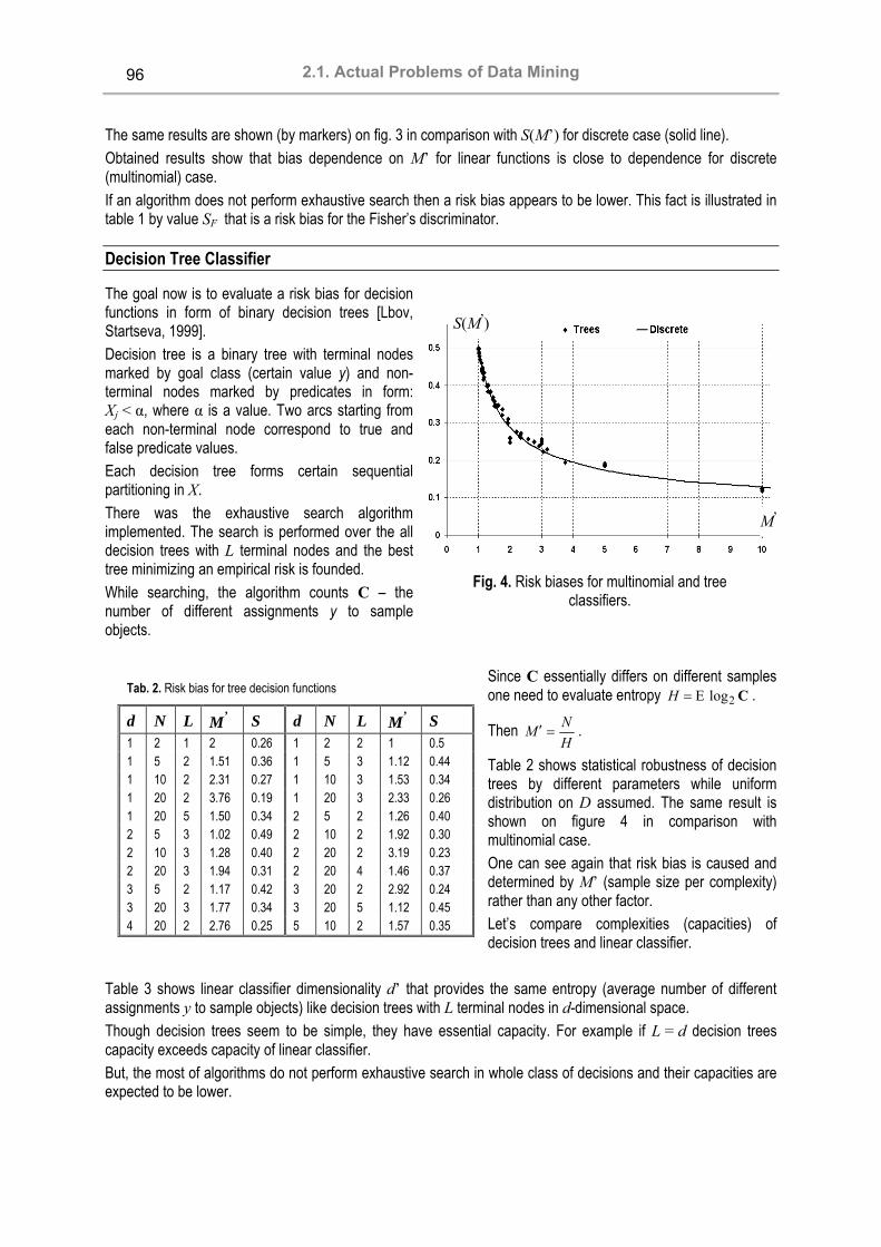
2.1. Actual Problems of Data Mining
96
The same results are shown (by markers) on fig. 3 in comparison with S(M’) for discrete case (solid line). Obtained results show that bias dependence on M’ for linear functions is close to dependence for discrete (multinomial) case. If an algorithm does not perform exhaustive search then a risk bias appears to be lower. This fact is illustrated in table 1 by value SF that is a risk bias for the Fisher’s discriminator.
Decision Tree Classifier
The goal now is to evaluate a risk bias for decision functions in form of binary decision trees [Lbov, Startseva, 1999]. Decision tree is a binary tree with terminal nodes marked by goal class (certain value y) and non-terminal nodes marked by predicates in form: Xj < α, where α is a value. Two arcs starting from each non-terminal node correspond to true and false predicate values. Each decision tree forms certain sequential partitioning in X. There was the exhaustive search algorithm implemented. The search is performed over the all decision trees with L terminal nodes and the best tree minimizing an empirical risk is founded. While searching, the algorithm counts C – the number of different assignments y to sample objects.
Since C essentially differs on different samples one need to evaluate entropy C2logE=H .
Then HNM =′ .
Table 2 shows statistical robustness of decision trees by different parameters while uniform distribution on D assumed. The same result is shown on figure 4 in comparison with multinomial case. One can see again that risk bias is caused and determined by M’ (sample size per complexity) rather than any other factor. Let’s compare complexities (capacities) of decision trees and linear classifier.
Table 3 shows linear classifier dimensionality d’ that provides the same entropy (average number of different assignments y to sample objects) like decision trees with L terminal nodes in d-dimensional space. Though decision trees seem to be simple, they have essential capacity. For example if L = d decision trees capacity exceeds capacity of linear classifier. But, the most of algorithms do not perform exhaustive search in whole class of decisions and their capacities are expected to be lower.
Tab. 2. Risk bias for tree decision functions
d N L M’ S d N L M’ S 1 2 1 2 0.26 1 2 2 1 0.5 1 5 2 1.51 0.36 1 5 3 1.12 0.44 1 10 2 2.31 0.27 1 10 3 1.53 0.34 1 20 2 3.76 0.19 1 20 3 2.33 0.26 1 20 5 1.50 0.34 2 5 2 1.26 0.40 2 5 3 1.02 0.49 2 10 2 1.92 0.30 2 10 3 1.28 0.40 2 20 2 3.19 0.23 2 20 3 1.94 0.31 2 20 4 1.46 0.37 3 5 2 1.17 0.42 3 20 2 2.92 0.24 3 20 3 1.77 0.34 3 20 5 1.12 0.45 4 20 2 2.76 0.25 5 10 2 1.57 0.35
Fig. 4. Risk biases for multinomial and tree classifiers.
S(M’)
M’

KDS 2005 Section 2: Data Mining and Knowledge Discovery
97
Note that if an algorithm implements good heuristic search and always founds the best decision function, then its capacity will be nevertheless equal to the capacity of exhaustive search algorithm. So, there is no use to count a number of decisions being really tested by an algorithm, because this number is irrelevant to actual capacity. Hence, calculation of effective capacity requires different approach. Effective algorithm capacity may be estimated by the following way. First one need to perform statistical modelling using uniform distribution on D. In this case misclassification probability (risk) equals to 0,5 for any decision function. Expectation of empirical risk is estimated by modelling, so risk bias is estimated too. Then via comparing the bias obtained by modelling with the bias for exhaustive search algorithm, the effective capacity of the algorithm under investigation is easily revealed.
Conclusion
Risk estimates by Vapnik and Chervonenkis are known to be excessively pessimistic. But the approach based on complexity measure is very attractive because of universality. The work presented shows that the reason for such pessimistic estimates is an inaccurate inference technique, but not the worst case orientation. So, it is possible to obtain estimates assuming the “worst” distribution and the ‘worst’ sample but these estimates will be appropriate in practice. For the multinomial case (a discrete feature) there was found how far Vapnik–Chervonenkis risk estimations are off. For continuous features the dependence of risk bias on complexity in considered cases is close to multinomial one that ensures a possibility to apply obtained scaling of VC-estimates to real tasks, e.g. linear decision functions and decision trees. The results obtained for multinomial case may be propagated on continuous one by using VC-capacity of decision function class instead of n. Comparison of linear classifier and decision trees capacities is also performed. There was also described a method for estimation an effective capacity of an algorithm that does not perform exhaustive search in the class of decision functions.
Bibliography
[Vapnik, Chervonenkis, 1974] Vapnik V.N., Chervonenkis A. Ja. Theory of pattern recognition. Moscow “Nauka”, 1974. 415p. (in Russian).
[Raudys, 2001] Raudys S., Statistical and neural classifiers, Springer, 2001. [Lbov, Startseva, 1999] Lbov G.S., Startseva N.G. Logical deciding functions and questions of statistical stability of
decisions. Novosibirsk: Institute of mathematics, 1999. 211 p. (in Russian). [Nedel’ko, 2003] Nedel’ko V.M. Estimating a Quality of Decision Function by Empirical Risk // LNAI 2734. Machine Learning
and Data Mining, MLDM 2003, Leipzig. Proceedings. Springer-Verlag. 2003. pp. 182–187.
Author's Information
Victor Mikhailovich Nedel’ko – Institute of Mathematics SB RAS, Laboratory of Data Analysis, 660090, pr. Koptyuga, 4, Novosibirsk, Russia, e-mail: [email protected]
Tab. 3. Correspondent dimensionality for tree and linear decision functions. Non-integer values of d’ appears because of interpolation performed.
d N L d' d N L d' 1 5 2 1 2 5 2 1.56 2 10 2 1.4 2 20 2 1.3 3 2 2 1 3 5 2 1.83 3 10 2 1.64 3 20 2 1.47 4 5 2 2.09 4 20 2 1.59 5 10 2 1.93 10 10 2 2.45 1 5 3 2 2 5 3 2.95 2 10 3 2.86 2 20 3 2.66 3 5 3 3.76 3 10 3 3.48 3 20 3 3.07 4 5 3 3.99 4 10 3 3.94 2 5 4 3.99 2 20 4 4.26 3 5 4 4 3 10 4 5.82 3 20 4 5.1 4 10 4 6.77 1 10 5 4 2 10 5 6.45 3 15 5 7.77

2.2. Structural-Predicate Models of Knowledge
98
2.2. Structural-Predicate Models of Knowledge
SCIT — UKRAINIAN SUPERCOMPUTER PROJECT
Valeriy Koval, Sergey Ryabchun, Volodymyr Savyak, Ivan Sergienko, Anatoliy Yakuba
Abstract: the paper describes a first supercomputer cluster project in Ukraine, its hardware, software and characteristics. The paper shows the performance results received on systems that were built. There are also shortly described software packages made by cluster users that have already made a return of investments into a cluster project.
Keywords: supercomputer, cluster, computer structure.
Introduction
To solve the most important tasks of an economy, technology, defense of Ukraine, that have large and giant computing dimensions, we need to be able to calculate extralarge information arrays. Such extremely large computations are impossible without modern high-performance supercomputers. Unfortunately, such computational resources are almost unavailable in Ukraine today. This can cause a precarious situation development in a different country's life areas. We can lose leading positions in a science, science intensive products' development, complex objects and processes modelling and design technologies. It is also impossible to import large supercomputers for the above mentioned tasks, because of embargo (for really powerful supercomputers), their extra-large prices, practically impossible upgrade, requirements to control the usage of imported supercomputers from abroad. In this situation Ukraine and other countries (India, China, Russia, Belarus) need to design its national supercomputers [1]. Today in Glushkov Institute of Cybernetics NAS of Ukraine, two high-performance and highly effective computational cluster systems SCIT-1 and SCIT-2 are running in an operation-testing mode. They are built on the basis of modern microprocessors INTEL® XEON™ и INTEL® ITANIUM® 2. On the basis of these supercomputer systems, a powerful joint computer resource will be built. It will be available for access for users from different organisations from different regions from all the NAS of Ukraine. The systems built are focused to applications from the fields of molecular biology, genetics, science of materials, solid-state physics, nuclear physics, semiconductor physics, astronomy, geology.
Development Ideology
While developing a supercomputer, system scientists and engineers face, a great amount of questions that requires to run a different kind of experiments. The experiments are run to understand a performance, features and characteristics of architecture, hardware platform for computing node solution, node interconnections, networking interfaces, storage system [2]. To make a right decision on system architecture we have made an analysis of world supercomputer tendencies. One of major sources we used was top500 list of the largest supercomputer installations. An analysis we made proves us, that a solution of cluster architecture is a right one. Cluster computer system – is a group of standard hardware and software components, coupled to solve tasks. Standard single processor or SMP (symmetric multiprocessor system) are used as processing elements in a cluster. Standard high-performance interconnect interfaces (Ethernet, Myrinet, SCI, Infiniband, Quadrics) are used to connect processing elements in a cluster system.

KDS 2005 Section 2: Data Mining and Knowledge Discovery
99
A development of supercomputer systems with cluster architecture is one of the most perspective ways in the world of high-performance computations today. The amount of supercomputer clusters installed in the world in increasing rapidly and the amount of finances spent for this direction is also increased. Tendencies of a development of supercomputers in the world for MPP (Massively Parallel Processing), PVP (Parallel Vector Processor) and cluster systems are shown on a Picture 1. As shown on the picture below, clusters are dominated in top500 list. For the several last years, an amount of cluster systems in the list have grown and an amount of MPP and PVP systems is going down.
When making a selection of a hardware platform of computational nodes we analyzed price/performance ratio. As LINPACK is rather narrow test, we choose SPECfp tests understand a performance of nodes on the basis of different kind of real applications. The prices we calculated were taken from Ukrainian IT market operators. The diagram received in analysis is shown on a Picture 2.
Picture 2. Price/performance ratio on the basis of SPECfp analysis
Today also new SPEChpc tests are available, that can give us an understanding of hpc computers performance for an applications from chemical, environment, seismic area and also OpenMP and MPI applications testing. Price/performance analysis is made with a calculation of costs of all the main components of a system and its environment with a focus on a theoretical peak 300 GFlops performance, which is near 120 000 SPECfp. We have also take into consideration performance downsize for different platforms scaling on the basis of self made tests.
Picture 1. World supercomputer tendencies
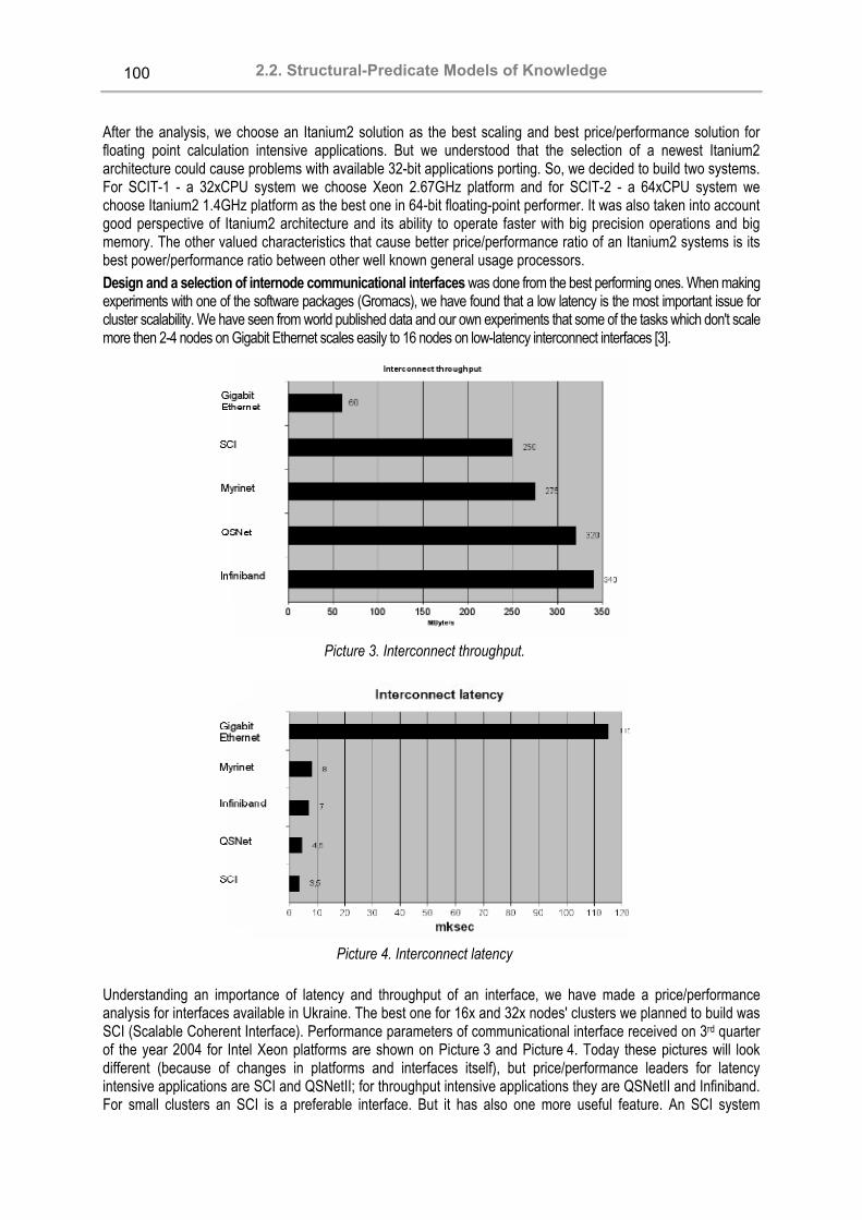
2.2. Structural-Predicate Models of Knowledge
100
After the analysis, we choose an Itanium2 solution as the best scaling and best price/performance solution for floating point calculation intensive applications. But we understood that the selection of a newest Itanium2 architecture could cause problems with available 32-bit applications porting. So, we decided to build two systems. For SCIT-1 - a 32xCPU system we choose Xeon 2.67GHz platform and for SCIT-2 - a 64xCPU system we choose Itanium2 1.4GHz platform as the best one in 64-bit floating-point performer. It was also taken into account good perspective of Itanium2 architecture and its ability to operate faster with big precision operations and big memory. The other valued characteristics that cause better price/performance ratio of an Itanium2 systems is its best power/performance ratio between other well known general usage processors. Design and a selection of internode communicational interfaces was done from the best performing ones. When making experiments with one of the software packages (Gromacs), we have found that a low latency is the most important issue for cluster scalability. We have seen from world published data and our own experiments that some of the tasks which don't scale more then 2-4 nodes on Gigabit Ethernet scales easily to 16 nodes on low-latency interconnect interfaces [3].
Understanding an importance of latency and throughput of an interface, we have made a price/performance analysis for interfaces available in Ukraine. The best one for 16x and 32x nodes' clusters we planned to build was SCI (Scalable Coherent Interface). Performance parameters of communicational interface received on 3rd quarter of the year 2004 for Intel Xeon platforms are shown on Picture 3 and Picture 4. Today these pictures will look different (because of changes in platforms and interfaces itself), but price/performance leaders for latency intensive applications are SCI and QSNetII; for throughput intensive applications they are QSNetII and Infiniband. For small clusters an SCI is a preferable interface. But it has also one more useful feature. An SCI system
Picture 3. Interconnect throughput.
Picture 4. Interconnect latency

KDS 2005 Section 2: Data Mining and Knowledge Discovery
101
network can be built on 2D mash topologies. Such architecture gives an ability to transfer data into two ways simultaneously. But to receive an advantage from this technology, software should be written with an understanding of this ability. It is known that performance and intelligence are the most important factors promoting the development of modern universal high-performance computers. The first factor forced a development of parallel architectures. The rational base of this development is universal microprocessors, connected into cluster system architectures. The second factor becomes clear when the notion of machine intellect (MI) is used. The concept of MI is introduced by V.M.Glushkov. MI defines “internal computer intelligence” and the term “intellectualisation” is used to define an increase of machine intellect. During the last 5-6 years, V.M.Glushkov Institute of Cybernetics NAS of Ukraine carries out the research aimed at the development of cluster based, knowledge-oriented architectures called intelligent solving machines (ISM). ISM implementing high- and super-high-level languages (HLL and SHLL) and effective operation with large-size data- and knowledge bases. They operate as with traditional computation tasks (mathematical physics, modelling of complex objects and processes, etc.) as artificial intelligence (AI) tasks (knowledge engineering, pattern recognition, diagnosis, forecasting) [4]. Large-size complex data- and knowledge bases in these clusters are displayed as oriented graphs of an arbitrary complexity – trees, semantic networks, time constrained, etc. In ISM computers it is possible to build graphs with millions nodes and to represent various knowledge domains. It is also important that the developed architecture can be easily integrated with distributed database architectures, which are developed in Glushkov Institute of Cybernetics NAS Ukraine. This database architecture makes search processes and data processing much faster than solutions with traditional architectures. The intellectual part of the cluster systems developed together with distributed databases is an advantage of this solution as compared with the systems developed in the other sites of the world. Hardware and software of the systems developed. Today the following SCIT (supercomputer for informational technologies) supercomputers are built in the institute (Picture 5):
Picture 5. Photo of SCIT clusters.
SCIT-1 – 32xCPU, 16xNodes cluster on the basis of Intel Xeon 2.67GHz 32-bit processors. They are oriented to operate with 64-bit and 128-bit data. The peak performance of SCIT-1 is 170 GFlops with an ability to be upgraded to 0,5-1 TFlops (right on a photo). SCIT-2 – 64xCPU, 32xNodes cluster on the basis of Intel Itanium2 1.4GHz 64-bit processors. They are oriented to operate with 128-bit and 256-bit data. The peak performance of SCIT-2 is 358 GFlops with an ability to be

2.2. Structural-Predicate Models of Knowledge
102
upgraded to 2,0-2,5 TFlops. The storage system has capacity of 1 TByte and ability to be upgraded to 10-15 TBytes (left on a photo). Each of two clusters is an array of computing nodes, connected together with three networks. The first one is a system network, based on SCI interface. The second one is a file data network, based on Gigabit Ethernet interface. The third one is a management network, based on Fast Ethernet interface. A general block-scheme of the SCIT supercomputer is shown on a Picture 6.
Picture 6. SCIT cluster structure.
A local data network is based on SCI and is used for a high-performance low-latency inter-node communication during a calculation process. A local data network is built as 2D mash. For 16x node cluster it is configured as 4x4 or 2x8 2D mash. For 32x node cluster it is configured as 4x8 or 2x16 2D mash. On data transfers based on MPI the throughput for Xeon E7501 platforms is 250 MB/s, for Itanium2 8870 platforms – 355 MB/s. A local control network is based on Gigabit Ethernet and is used to handle all cluster-computing nodes and to transfer data files between nodes and file server. A local monitor network is used for service information transfer and monitoring of all the cluster system. On a table 1 performance parameters of SCIT-1 and SCIT-2 systems are described.
Table 1. 64-bit performance parameters of SCIT-1 and SCIT-2 systems. SCIT-1 SCIT-2 1 Processors P-IV Xeon 2,67 GHz Itanium2 1,4 GHz 2 Peak performance of a single processor Integer operations per second, 10 9IPS 1,34 5,6 Floating point operations per second, GFLOPS 5,34 5,6 Node system bus performance, GB/s 4,2 6,4 3 Total peak performance of a system Integer operations per second, 10 9IPS 43 358 Floating point operations per second, GFLOPS 170 358 Total system bus performance, GB/s 67,2 204,8 4 Linpack performance of a system, GFLOPS 112,5 280
controlnode
local control networkGigabit Ethernet, Star Topology
local data networkSCI, 2D Mash Topology
localmonitornetwork
FastEthernet,
TreeTopology
computingnode
...computing
nodecomputing
node
gatewayfile server

KDS 2005 Section 2: Data Mining and Knowledge Discovery
103
Performance characteristics of developed systems SCIT-1 and SCIT-2 are on the one stage with world best systems. They are also one of the best systems in a world mathematical supercomputing construction. The creation of cluster systems SCIT-1 and SCIT-2 and their integration and finally launch was made due to a fruitful cooperation of Glushkov Institute of Cybernetics NAS of Ukraine with USTAR scientific and manufacturing company (based in Kiev) and Intel corporation (International). The partners of the institute delivered a technical support and consulting of a project.
System Level Software
Components of system level software of a cluster support all stages of user-level parallel software development. They also provide execution of users processes of substantial processing on a solving field. They run on all the nodes of a cluster and a control node as well. Operating system used are ALT Linux for SCIT-1 and Red Hat Enterprise Linux AS for SCIT-2. Message Passing Interface (MPI) over SCI is used for programming in a message-passing model. In addition, system level software includes optimized compilers of C, C++, Fortran languages for parallel programming, fast Math libraries, etc.
Application Level Software
The powerful hardware, system level, service and specific cluster software integrated in a system is a strong ground for an application level software development. It gives an ability to solve new extra large tasks in a fields of science, economy, ecology, agriculture, technology, defense, space industry, etc. Due to successful implementations of SCIT systems for the several months after the system was installed a lot of applications were developed and deployed on a supercomputer in Glushkov Institute of Cybernetics NAS of Ukraine. The software packages for the following tasks were developed: • soil ecology problems solution; • seismic data processing; • dynamical travelling salesman in a real time; • modelling a structural-technological changes in a developing economy; • a search for an optimal service center placement; • construction of an interference-tolerant code; • risk classification and evaluation decisions; • data clusterization with genetics algorithms; • decomposition, calculation, verification and solving of a theorems; • software component for linear algebra; • low-energy orbit selection; • software package for a natural and technogenic processes analysis.
Conclusion
The supercomputer cluster project, as a first stage of a national supercomputer resources development, made a great impact on an intellectualisation of information technologies in Ukraine. The next stage will be devoted to improvement of performance characteristics of supercomputers designed and their software. This should allow extending an amount of large complex tasks that would be solved on the systems.
Bibliography
1. Koval V.N., Savyak V.V., Sergienko I.V., “Tendencies of modern supercomputer systems development”, Control Systems and Computers, Vol.6, November-December 2004, 31-44 pp (In Russian).
2. Koval V.N., Savyak V.V., “Multiprocessor cluster systems: planning and implementation”, “Nauka osvita”, Artificial Intellect, Vol.3, 2004, 117-126 pp (In Russian).

2.2. Structural-Predicate Models of Knowledge
104
3. www.gromacs.org 4. Koval V., Bulavenko O, Rabinovich Z Parallel Architectures and Their Development on the Basis of Intelligent Solving
Machines // Proc. Int. Conf. on Parallel Computing in Electrical Engineering. — Warsaw (Poland).- 2002.- P.21-26
Authors' Information
Valeriy N. Koval – Institute of Cybernetics NAS Ukraine; Prospekt Academika Glushkova,40, Kiev, 03680 MCP, Ukraine; email: [email protected] Volodymyr V. Savyak – Institute of Cybernetics NAS Ukraine; Prospekt Academika Glushkova,40, Kiev, 03680 MCP, Ukraine; email: [email protected] Ivan V. Sergienko – Institute of Cybernetics NAS Ukraine; Prospekt Academika Glushkova,40, Kiev, 03680 MCP, Ukraine Sergey G. Ryabchun – Ustar Corp. ; office 1, 16A, Dovzhenko str., Kiev, 03057, Ukraine; email: [email protected] Anatoliy A. Yakuba – Institute of Cybernetics NAS Ukraine; Prospekt Academika Glushkova, 40, Kiev, 03680 MCP, Ukraine; email: [email protected]
DISCOVERY OF NEW KNOWLEDGE IN STRUCTURAL-PREDICATE MODELS OF KNOWLEDGE
Valeriy N. Koval, Yuriy V. Kuk Abstract: The effective mathematical method of finding new knowledge of structure of complex objects with required properties is developed. The method comprehensively takes into account the information on properties and relations of the primary objects, which are included in complex objects. It is based on measurement of distances between groups of predicates at their some interpretation. The optimum measure for measurement of these distances with the maximal discernibleness of different groups of predicates is constructed. The method is approved on the decision of a problem of discovery of the new compound possessing electrooptical properties.
Keywords: new knowledge, predicates, measure, complex objects, primary objects, maximal discernibleness.
Introduction
The given work is devoted to the further development of methods of practical extraction of knowledge from experimental data. Its purpose - development of an effective mathematical method of discovery of new knowledge of structure of the complex objects possessing those or other properties. Work is focused on the decision of the important applied problem - designing of structure of compound with the necessary properties. In previous our works [1] - [2] for discovery of new knowledge in the form production rules the concept of a variable predicate which can accept set of values - so-called predicate constants - predicates in the standard sense and the concept of distance between predicates were used. These both concepts have received the further development in the present work. However as against the above mentioned works in given article predicates with the subject domains consisting of objects, having internal structure are considered, that is objects from subject domains of predicates are assumed complex while earlier they were considered integral. Components of complex object we shall name primary objects [3], and the predicates designating properties and the relations of primary objects, we shall name primary predicates. About properties and relations of the primary objects included of complex objects, as a rule, also some information, which should be used in procedures of discovery of new knowledge of structure of the complex objects possessing those or other properties, is known. Procedure of discovery of such knowledge suggested in work is based on measurement of distances between groups of properties and relations of primary objects, or in language of logic, between groups of predicates at their some interpretation. The measure entered by us in works [1] - [2] for measurement of a degree of affinity of predicates,

KDS 2005 Section 2: Data Mining and Knowledge Discovery
105
cannot be directly transferred on groups of predicates. Therefore, in the given work the special measure, optimum by criterion of the maximal discernibleness of different groups of predicates, for measurement of distances between them is entered.
1. Structural-predicate Model of Knowledge
It is conveniently knowledge of complex objects to represent in the form which we have named structural - predicate model of knowledge. It is the further generalization of structural - attributive model of knowledge [3]-[4]. Generalization will be, that their relations, and not just properties of objects are considered also. For example, the two-place predicate « a difference of temperatures of fusion of two substances more ∆ » describes some relation between two objects. The structural - predicate model of knowledge (SPMK) is four-layer columns of a pyramidal network which separate layers form its tops. For presentation on fig. 1 it is resulted SPMK, containing knowledge of properties of chemical compounds with various types of structures of a crystal lattice: such as LiCaAlF6 (L-structure of a lattice), such as Na2SiF6 (N-structure of a lattice), such as Trirutile (T-structure of a lattice). We shall designate P , A , S , V the following sets of tops SPMK. The first layer P corresponds to predicate constants (values of variable predicates), designating properties and relations of primary objects. Elements P we shall name primary predicates. On fig. 1 primary variable predicates are: Tm - a melting point, So - standard entropy for corresponding simple oxides, H - standard enthalpy formations for corresponding simple oxides, Rs - radius of ions, C - an isobaric thermal capacity. On fig. 1 each of these predicates accepts on 2 values, and predicate constants corresponding to them are designated by numbers 1 and 2.
Fig. 1 the Example of structural - predicate model of knowledge
The second layer A corresponds to names of primary objects. They make subject domains of primary predicates at their interpretation. The third layer S corresponds to names of compound objects, the fourth V - to values of the variable predicates designating properties and the relations of compound objects. Elements V we shall name predicates of compound objects. Their subject domains are compound objects. On fig. 1 predicates of compound objects are 3 values of a variable predicate «to have the certain type of a crystal lattice». Arches of the bottom and top circles connect the tops representing objects, to the tops, representing predicate constants, and are directed from primary and compound objects to predicate constants. They are used at interpretation of predicates. Let ω designates multiplicity of some predicate constant. Then presence ω of the arches proceeding from ω objects and converging in the given predicate, corresponds to logic value of a predicate "true" at substitution of these objects in a predicate, and to value "lie" - at substitution of object in a predicate in a case absence of the arch, connecting given object with a predicate. Thus, at substitution of objects A and S from which to predicate constants arrows proceed from sets P and V , instead of arguments of these predicate
CrF3 AlF3 LiF InF3 VF3 MnF2 TiF3 CaF2 NiF2
LiCaInF6 LiCaCrF6 LiNiVF6 LiNiTiF6 LiMnTiF6 LiCaAlF6
L- structure of a lattice
N- structure of a lattice
T- structure of a lattice
Tm1 Tm2 So1 So2 H1 H2 Rs1 Rs2 C1 C2

2.2. Structural-Predicate Models of Knowledge
106
constants two sets of knowledge 1R and 2R in the form of true statements about properties and relations of primary and compound objects are formed. Arches of an average circle connect the tops corresponding to primary objects, to the tops representing compound. Primary elements, from which arches proceed, are part of those complex objects in which these arches comes to an end.
2. A Measure of Affinity of Groups of Predicates
Let's consider a problem of construction of a measure for measurement of a degree of affinity of groups of variable predicates. This measure should possess the following natural property: the distance between groups of the predicates, measured with its help, should not be equal to zero when these groups of predicates are various. From here follows, that it should possess property of the maximal discernibleness of different groups of predicates. We shall construct a measure satisfying this property. Let's designate N - number of primary predicates in structural - predicate model, M - number of predicates of compound objects, )(kn - number of the primary objects, which are included in complex object ks . Symbols
Npp L,1 we shall designate primary variable predicates of model. In case of numerical values of variable predicates we shall adhere to the following rule: indexes for their predicate constants get out so that the order of their following corresponded to the order of following of numerical values of variable predicates. Thus, at dividing an interval of change of numerical values of predicates into segments (digitization), indexes of predicate constants, which correspond to them, should coincide with numbers of these segments. Definition 1. The label ikx of a primary variable predicate ip for complex object ks is understood as an index of that predicate constant of a predicate ip which accepts logic value "True" at substitution in it instead of arguments of the primary objects included in ks and connected by arches with this predicate constant. Distribution of labels ),,,( 21 Nkkkk xxxx L= of primary predicates for compound ks we shall name a vector which elements are labels for complex object ks of all primary predicates which are included in structural - predicate model of knowledge. Typical distribution of labels for group of complex objects
)1()1(2
)1(11 ,,, KsssG L= we shall name a vector ),,,( )1()1(
2)1(
1)1(
Nxxxh L= which coordinates are equal to average values of components of vectors of labels in the group. We shall name a vector
),,,(~ 1122
111 NNkkkk xxxxxxx −−−= L a centralized vector of labels of primary predicates for the complex
object ks belonging to group of complex objects )1()1(2
)1(11 ,,, KsssG L= .
Distributions of labels of primary predicates for some group of complex objects represent set of points in space NR . If there are two groups of complex objects, we shall receive two such sets of points, which are mixed
among them in a random way. There is a following problem: it is required to find such characteristics of these sets that it was possible to measure a degree of affinity of groups with their help. The following decision arises: to take as characteristics of each of sets of points corresponding points with the average coordinates which represent that other as typical distribution of labels for corresponding groups, and Euclidean length of distance between them to take as a measure of affinity for these groups. However, this decision is not optimum. Really, we shall consider the following example. Let points of distributions of labels of primary predicates for both groups are located on two perpendicular straight lines symmetrically concerning their center of crossing, and points of each group lay on a separate line. It is easy to see, that typical distributions of labels for both groups will coincide, and, hence, the distance between them is equal to zero though groups of predicates are various. It is possible to look at the above-stated not optimum decision from other point of view, allowing finding the optimum decision. We shall lead a direct line through two points which are in NR typical distributions of labels of primary predicates for complex objects of both groups, and we shall project on it sets of points for both groups. It is easy to see that average values of projections for both sets of points, the so-called centers of projections 1z and 2z corresponding groups, coincide with the points representing typical distributions of labels. As the measure should possess property of the maximal discernibleness of different groups of predicates from here there is a following optimization problem: to construct in NR the direct line c which is not necessarily taking place through typical

KDS 2005 Section 2: Data Mining and Knowledge Discovery
107
distributions labels, such that the distance center to center projections of both sets of points was maximal. The criterion of optimization of the given problem looks like: max21 →− zz . The distance 21 zz − received as a result of optimization should be taken as a measure of affinity of complex objects for both groups.
3. The Mathematical Apparatus for Constructing the Measure
From the previous section follows, that for finding the optimum decision of a problem of construction of a measure for measurement of a degree of affinity of groups of variable predicates it is necessary to construct some auxiliary direct line c in space NR and to project distributions of labels for both groups of predicates on it. In result, we shall receive two crossed sets of points on a direct line. As the choice of a direction of a line c influences distances between projections of distributions of labels and, hence, on their affinity the direct line should be chosen so that projections of distributions of labels from different groups of complex objects would be removed from each other so far as far as it is possible. Such choice of a direction of a line will allow distinguishing different groups of complex objects in the optimum way. A direct line c , on which distributions of labels of primary predicates for complex objects are projected, we shall name a projective line. Let's result without the proof a number of auxiliary statements necessary for finding the required projective line. Lemma 1. The projection of distributions of labels ),,,( 21 Nkkkk xxxx L= of primary predicates for complex object ks to the projective line c , which is taking place through the beginning of coordinates in space NR , is
defined by the formula 12121111Pr NNc xcxcxcx +++= L , where ),,,( 21 Nccc L - cosines of the corners formed by a straight line with axes of coordinates. Definition 2. Disorder concerning any point z of projections of distributions of labels of primary predicates for group of complex objects )1()1(
2)1(
11 ,,, KsssG L= we shall name total distance )(1 zD .
∑=
−=K
zzzD1
)1(1 )(
νν , where )1(
1)1(
111)1(
1 NN xcxcz ++= L ,…, )1()1(11
)1(NKNKK xcxcz ++= L .
The center of projections for group of complex objects )1()1(2
)1(11 ,,, KsssG L= we shall name average value of
projections of distributions of labels of primary predicates for group 1G : ∑=
=K
zK
z1
)1()1( 1
νν .
Lemma 2. The disorder concerning any point z of projections of distributions of labels of primary predicates for group of complex objects )1()1(
2)1(
11 ,,, KsssG L= is minimal, when z is equal to the center of their
projections: )1(zz = , thus ∑=
−==K
zzzDzD1
2)1()1(11 )()()(
νν .
Let )1()1(2
)1(11 ,,, KsssG L= and )2()2(
2)2(
12 ,,, LsssG L= - two groups of the complex objects consisting accordingly from K and L complex objects. For each complex object of these groups, we shall construct on the basis of structural - predicate model of knowledge distribution of labels of its primary predicates. We shall receive
LK + vectors, which in space NR will be displayed by two sets of vectors: 1X - set of vectors )1(1x )1(
2x , …, )1(
Kx and 2X - set of vectors )2(1x )2(
2x , … )2(Lx . We shall project sets 1X and 2X on a projective line c .
On the basis of a lemma 1, we shall find values of projections: )1(1
)1(212
)1(111
)1(1
)1(1 Pr NNc xcxcxcxz +++== L , …, )2(
1)2(
212)2(
111)2(
1)2(
1 Pr NNc xcxcxcxz +++== L ,
)2(2
)2(222
)2(121
)2(2
)2(2 Pr NNc xcxcxcxz +++== L , … )2()2(
22)2(
11)2()2( Pr NLNLLLcL xcxcxcxz +++== L .
Let's designate sets of projections 1X and 2X accordingly 1Z and 2Z , and their centers:

2.2. Structural-Predicate Models of Knowledge
108
)(1 )1()1(2
)1(1
)1(Kzzz
Kz +++= L , )(1 )2()2(
2)2(
1)2(
LzzzL
z +++= L .
Definition 3. Disorder concerning an any point z of projections of distributions of labels of primary predicates for the pooled group of complex objects 21 GGG U= we shall name the general disorder of both groups )(zD .
It is obvious, that it is equal ∑∑==
−+−=LK
zzzzzD1
)2(
1
)1()(ν
νν
ν . The general center of the pooled set of
projections 21 ZZZ U= we shall name size )(1 )2()2(1
)1()1(1 LK zzzz
LKz +++++
+= LL .
Let's result without the proof the following theorem about the disorder of projections of distributions of labels of primary predicates. Theorem 1. The general disorder )(zDD = concerning the general center z of projections of distributions of labels of primary predicates of the pooled group of complex objects 21 GGG U= is calculated under the formula 2121 ˆˆ DDDDD +++= , where
∑=
−=K
zzD1
2)1()1(1 )(
νν , ∑
=−=
LzzD
1
2)2()2(2 )(
νν , 21
1 )(ˆ zzKD −= , 2)2(2 )(ˆ zzLD −= .
From the theorem 1 follows that to maximize a measure of discernibleness of both groups of predicates - distance 21 zz − it is necessary to maximize the sum 21
1 )(ˆ zzKD −= and 222 )(ˆ zzLD −= . We shall name the
sum 21 DD + full discernibleness . We shall receive expressions for the full discernibleness and the sums of disorders of projections of distributions of labels of both groups of predicates, which are used at the further calculations. Vector of a difference of typical distributions of labels for groups of complex objects 1G also 2G we shall
designate ),,,( )2()1()2(2
)1(2
)2(1
)1(1
)2()1(NN xxxxxxhhh −−−==−= L .
Let's construct a square matrix hhH T= where the top index T designates operation of transposing. Dimension H is equal NN × . It looks like
⎟⎟⎟⎟⎟
⎠
⎞
⎜⎜⎜⎜⎜
⎝
⎛
−−−−−
−−−−−
−−−−−
=
2)2()1()2(2
)1(2
)2()1()2(1
)1(1
)2()1(
)2()1()2(2
)1(2
2)2(2
)1(2
)2(1
)1(1
)2(2
)1(2
)2()1()2(1
)1(1
)2(2
)1(2
)2(1
)1(1
2)2(1
)1(1
)())(())((
))(()())((
))(())(()(
NNNNNN
NN
NN
xxxxxxxxxx
xxxxxxxxxx
xxxxxxxxxx
H
L
LLLL
L
L
.
Let's consider a matrix H ′ with elements ),(),( µνµν hLK
KLh+
=′ and designate )1(A and )2(A matrixes
which columns will consist of components centralized distributions of labels of primary predicates for corresponding groups of complex objects. They contain N lines and accordingly K and L columns.
⎟⎟⎟⎟
⎠
⎞
⎜⎜⎜⎜
⎝
⎛
−−
−−=
)1()1(11
11
)1()1(1
)1(1
)1(11
)1(
KNKN
KK
xxxx
xxxxA
L
LLL
L
, ⎟⎟⎟⎟
⎠
⎞
⎜⎜⎜⎜
⎝
⎛
−−
−−=
)2()2()2(1
)2(1
)2()2(1
)2(1
)2(11
)2(
LNLN
lKL
xxxx
xxxxA
L
LLL
L
Let's consider matrixes T
AAB )1()1()1( = and T
AAB )2()2()2( = . They look like:

KDS 2005 Section 2: Data Mining and Knowledge Discovery
109
⎟⎟⎟⎟⎟⎟⎟
⎠
⎞
⎜⎜⎜⎜⎜⎜⎜
⎝
⎛
−−−−−
−−−−−
=
∑∑∑
∑∑∑
===
===
K
NN
K
NN
K
NN
K
NN
KK
xxxxxxxxxx
xxxxxxxxxx
B
1
2)1()1(
1
)1(2
)1(2
)1()1(
1
)1(1
)1(1
)1()1(
1
)1()1()1(1
)1(1
1
)1(2
)1(2
)1(1
)1(1
1
2)1(1
)1(1
)1(
)())(())((
))(())(()(
νν
ννν
ννν
ννν
ννν
νν
L
LLLL
L
,
⎟⎟⎟⎟⎟⎟⎟
⎠
⎞
⎜⎜⎜⎜⎜⎜⎜
⎝
⎛
−−−−−
−−−−−
=
∑∑∑
∑∑∑
===
===
L
NN
L
NN
L
NN
L
NN
LL
xxxxxxxxxx
xxxxxxxxxx
B
1
2)1()1(
1
)1(2
)1(2
)1()1(
1
)1(1
)1(1
)1()1(
1
)1()1()1(1
)1(1
1
)1(2
)1(2
)1(1
)1(1
1
2)1(1
)1(1
)2(
)())(())((
))(())(()(
νν
ννν
ννν
ννν
ννν
νν
L
LLLL
L
In the following theorems, the formulas for calculation of the full discernibleness and the sum 21 DD + of disorders are resulted. The theorems we shall result without the proof. Theorem 2. The full discernibleness is equal
∑ ∑= =+
=+N N
hccLK
KLDD1 1
21 ),(ˆˆν µ
µν µν ,
where ),( µνh - the element of a matrix H which is taking place in a ν line and in a µ column.
Theorem 3. The sum of disorders of projections for distributions of labels of primary predicates 21 DD + is
equal ∑ ∑= =
=+N N
bccDD1 1
21 ),(ν µ
µν µν , where ),( µνb - elements of a matrix )2()1( BBB += .
We shall result without the proof the basic theorem, which allows distinguishing groups of predicates thus that full discernibleness was so big as far as, it is possible. Theorem 4. The full discernibleness 21 ˆˆ DD + reaches the maximum at the fixed value of the sum of disorders of groups when values cosines ),,,( 21 Nccc L of the corners formed by the projective line with axes of coordinates are the components of an eigen vector W for a nonzero eigen value of a matrix HB ′−1 .
6. Stages of Designing Structure of Complex Objects
Let's consider stages of the decision of a problem on designing structure of compounds with the set properties [3]. For presentation with this decision we shall accompany an example based on the data, resulted in [4]. Let it is required to design the new compounds possessing electrooptical properties. It is known, that electrooptical property crystals of fluorides, which have crystal structures of types LiCaAlF6 and Na2SiF6 possess, and the crystals of fluorides having structure such as Trirutile by such properties do not possess. For simplicity, we shall be limited to consideration of compounds with structures such as Na2SiF6 and Trirutile. At the first design stage SPMK, describing properties of compounds of fluorides, is under construction. The fragment of such model is resulted on fig. 1. At the second stage in SPMK the set of predicate constants of compound objects – +V to which there correspond required properties of projected compound, and set of predicate constants to which there correspond undesirable properties of projected compound is allocated – −V . In our example +V is a predicate «to have structure such as Na2SiF6», and −V is a predicate «to have structure such as Trirutile». At the third stage in SPMK the set of tops of the group 1G corresponding to known compounds which have connections with predicates of set +V is allocated, and have no connections with predicates of set −V , and set of the tops
2G corresponding to known compounds which have connections with predicates of set −V , and have no connections with predicates of set +V . Let the first group included 10 compounds which are resulted in the first column of the table 1, and the second group included 17 compounds resulted in the first column of table 2.
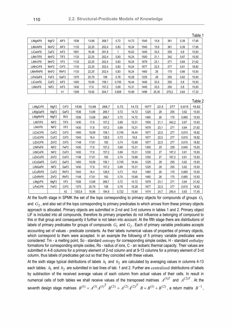
2.2. Structural-Predicate Models of Knowledge
110
Table 1 LiMgAlF6 MgF2 AlF3 1536 13,68 268,7 0,72 14,72 1545 15,8 361 0,39 17,95
LiMnAlF6 MnF2 AlF3 1133 22,25 202,4 0,83 16,24 1545 15,8 361 0,39 17,95 LiCaInF6 CaF2 InF3 1691 16,36 291,8 1 16,02 1445 33,5 250 0,8 15,93 LiMnTiF6 MnF2 TiF3 1133 22,25 202,4 0,83 16,24 1500 21,1 342 0,67 15,93 LiMnVF6 MnF2 VF3 1133 22,25 202,4 0,83 16,24 1679 23,1 271 0,64 21,62 LiMnCrF6 MnF2 CrF3 1133 22,25 202,4 0,83 16,24 1677 22,5 277 0,61 18,82 LiMnRhlF6 MnF2 RhF3 1133 22,25 202,4 0,83 16,24 1460 26 175 0,66 15,93
LiFeGaF6 FeF2 GaF3 1375 20,79 158 0,78 16,28 1225 28 255 0,62 15,93 LiCoInF6 CoF2 InF3 1400 19,59 159,1 0,745 16,44 1445 33,5 250 0,8 15,93 LiNiInF6 NiF2 InF3 1430 17,6 157,2 0,69 15,31 1445 33,5 250 0,8 15,93
h1 1309 19,92 204,7 0,808 15,99 1496 25,30 279,2 0,64 17,33
Table 2 LiMgCrF6 MgF2 CrF3 1536 13,68 268,7 0,72 14,72 1677 22,5 277 0,615 18,82 LiMgGaF6 MgF2 GaF3 1536 13,68 268,7 0,72 14,72 1225 28 255 0,62 15,93 LiMgRhF6 MgF2 Rh3 1536 13,68 268,7 0,72 14,72 1460 26 175 0,665 15,93 LiNiTiF6 NiF2 TiF3 1430 17,6 157,2 0,69 15,31 1500 21,1 342,2 0,67 15,93 LiNiVF6 NiF2 VF3 1430 17,6 157,2 0,69 15,31 1679 23,1 271 0,64 21,62
LiCoCrF6 CoF2 CrF3 1400 19,59 159,1 0,745 16,44 1677 22,5 277 0,615 18,82 LiCuCrF6 CuF2 CrF3 1043 16,4 128,5 0,73 16,8 1677 22,5 277 0,615 18,82 LiZnCrF6 ZnF2 CrF3 1148 17,61 183 0,74 15,69 1677 22,5 277 0,615 18,82 LiNiFeF6 NiF2 FeF3 1430 17,6 157,2 0,69 15,31 1300 25 239 0,645 15,93 LiNiCoF6 NiF2 CoF3 1430 17,6 157,2 0,69 15,31 1230 27 187,2 0,61 15,93 LiZnCoF6 ZnF2 CoF3 1148 17,61 183 0,74 15,69 1230 27 187,2 0,61 15,93 LiCoGaF6 CoF2 GaF3 1400 19,59 159,1 0,745 16,44 1225 28 255 0,62 15,93 LiNiGaF6 NiF2 GaF3 1430 17,6 157,2 0,69 15,31 1225 28 255 0,62 15,93 LiCuRhF6 CuF2 RhF3 1043 16,4 128,5 0,73 16,8 1460 26 175 0,665 15,93 LiZnRhF6 ZnF2 RhF3 1148 17,61 183 0,74 15,69 1460 26 175 0,665 15,93 LiMgVF6 MgF2 VF3 1536 13,68 268,7 0,72 14,72 1679 23,1 271 0,64 21,62 LiFeCrF6 FeF2 CrF3 1375 20,79 158 0,78 16,28 1677 22,5 277 0,615 18,82
h2 1352,8 16,96 184,9 0,722 15,60 1474 24,7 245,4 0,63 17,45
At the fourth stage in SPMK the set of the tops corresponding to primary objects for compounds of groups 1G and 2G , and also set of the tops corresponding to primary predicates to which arrows from these primary objects approach is allocated. Primary objects are submitted in 2-nd and 3-rd columns in tables 1 and 2. Primary object LiF is included into all compounds, therefore its primary properties do not influence a belonging of compound to this or that group and consequently it further is not taken into account. At the fifth stage there are distributions of labels of primary predicates for groups of compounds 1G and 2G . Each of primary variable predicates accepts accounting set of values - predicate constants. As their labels numerical values of properties of primary objects, which correspond to them were accepted. In an example the following of 5 primary variable predicates were considered: Tm - a melting point, So - standard entropy for corresponding simple oxides, H - standard enthalpy formations for corresponding simple oxides, Rs - radius of ions, C - an isobaric thermal capacity. Their values are submitted in 4-8 columns for a primary element of 2-nd column and at 9-13 columns for a primary element of 3-rd column, thus labels of predicates get out so that they coincided with these values. At the sixth stage typical distributions of labels 1h and 2h are calculated by averaging values in columns 4-13 each tables. 1h and 2h are submitted in last lines of tab. 1 and 2. Further are centralized distributions of labels by subtraction of the received average values of each column from actual values of their cells. In result in numerical cells of both tables we shall receive values of the transposed matrixes TA )1( and TA )2( . At the
seventh design stage matrixes T
AAB )1()1()1( =T
AAB )2()2()2( = )2()1( BBB += , a return matrix 1−B ,

KDS 2005 Section 2: Data Mining and Knowledge Discovery
111
and matrixes )()( )2()1()2()1( hhhhH T −−= and LK
KLHH+
=′ * , where 10=K , 17=L are calculated.
At the eighth stage, there is an eigen vector W for a nonzero eigen value of a matrix HB ′−1 (for example, with the help of program Matlab). For a considered example an eigen vector looks like == ),,,( 1021 cccW L (-0.0002 0.0359 0.0017 0.6283 -0.0276 0.0004 0.0363 0.0015 -0.7754 -0.0242). Cosines of the corners formed by an optimum projective line c with coordinate corners are proportional to values of this vector; thus, the coefficient of proportionality does not play any role. At the ninth stage, there are projections of typical distributions of labels to this line: ThWz 1
)1( *= and ThWz 2)2( *= . We have 889.1)1( =z , 6201.1)2( =z . Their common center
is equal 7545.1)(5.0 )2()1( =−= zzz . At the tenth stage gets out in SPMK primary objects for projected compound as follows. The objects having connections with primary predicates with which have also connections primary objects of group of compounds 1G get out, and there are no connections with primary predicates with which have connections primary objects of group of compounds 2G , thus possible restrictions on structure of compounds are taken into account. We shall assume that the compounds submitted in table 3 have been chosen.
Table 3 LiMgInF6 MgF2 InF3 1536 13,68 268,7 0,72 14,72 1445 33,5 250 0,8 15,93 LiMnFeF6 MnF2 FeF3 1133 22,25 202,4 0,83 16,24 1300 25 239 0,645 15,93 LiMnGaF6 MnF2 GaF3 1133 22,25 202,4 0,83 16,24 1225 28 255 0,62 15,93 LiMnInF6 MnF2 InF3 1133 22,25 202,4 0,83 16,24 1445 33,5 250 0,8 15,93 LiZnInF6 ZnF2 InF3 1148 17,61 183 0,74 15,69 1445 33,5 250 0,8 15,93 LiCdInF6 CdF2 InF3 1345 20 167,4 0,95 15,93 1445 33,5 250 0,8 15,93 LiMgTiF6 MgF2 TiF3 1536 13,68 268,7 0,72 14,72 1500 21,1 342,2 0,67 15,93 LiMgFeF6 MgF2 FeF3 1536 13,68 268,7 0,72 14,72 1300 25 239 0,645 15,93 LiMgCoF6 MgF2 CoF3 1536 13,68 268,7 0,72 14,72 1230 27 187,2 0,61 15,93 LiFeTiF6 FeF2 TiF3 1375 20,79 158 0,78 16,28 1500 21,1 342,2 0,67 15,93 LiCoTiF6 CoF2 TiF3 1400 19,59 159,1 0,745 16,44 1500 21,1 342,2 0,67 15,93 LiZnTiF6 ZnF2 TiF3 1148 17,61 183 0,74 15,69 1500 21,1 342,2 0,67 15,93 LiZnVF6 ZnF2 VF3 1148 17,61 183 0,74 15,69 1679 23,18 271 0,64 21,62 LiNiCrF6 NiF2 CrF3 1430 17,6 157,2 0,69 15,31 1677 22,5 277 0,615 18,82 LiFeFeF6 FeF2 FeF3 1375 20,79 158 0,78 16,28 1300 25 239 0,645 15,93 LiCoFeF6 CoF2 FeF3 1400 19,59 159,1 0,745 16,44 1300 25 239 0,645 15,93 LiCuFeF6 CuF2 FeF3 1043 16,4 128,5 0,73 16,8 1300 25 239 0,645 15,93 LiZnFeF6 ZnF2 FeF3 1148 17,61 183 0,74 15,69 1300 25 239 0,645 15,93 LiCuCoF6 CuF2 CoF3 1043 16,4 128,5 0,73 16,8 1230 27 187,2 0,61 15,93 LiCoRhF6 CoF2 RhF3 1400 19,59 159,1 0,745 16,44 1460 26 175 0,665 15,93 LiNiRhF6 NiF2 RhF3 1430 17,6 157,2 0,69 15,31 1460 26 175 0,665 15,93 LiCuGaF6 CuF2 GaF3 1043 16,4 128,5 0,73 16,8 1225 28 255 0,62 15,93
For check of correctness of a choice, the projection )3()3(22
)3(11z NN xсxсxс +++= L of distribution of labels
of each chosen connection to a projective straight line is calculated. If zzzz −<− )2()1( , than the choice is
considered correct. For compounds of table 3 consistently from top to down we find: z equally 1.8395, 1.9060, 2.0089, 2.1339, 1.8838, 2.0870, 1.6272, 1.6115, 1.5784, 1.7448, 1.6329, 1.6715, 1.6521, 1.6135, 1.7291, 1.6173, 1.5107, 1.6558, 1.4776, 1.5440, 1.4934, 1.6136. As 889.1)1( =z , 6201.1)2( =z only the first 6 compounds according to the given technique are chosen correctly, and the others it is erroneous. The considered example allows to check up also correctness of the technique as the structure of a lattice of compounds of table 3 is beforehand known: the first 6 compounds have structure of a crystal lattice such as Na2SiF6, and all subsequent chemical compounds have structure of a crystal lattice such as Trirutile. Thus, we receive 100 % of right answers that proves a technique while in work [4] 86,4 % of right answers for the same group of chemical compounds are received.

2.2. Structural-Predicate Models of Knowledge
112
Conclusion
In work complex objects with internal structure are considered. The structural - predicate model of knowledge, which is generalization of structural - attributive model of knowledge is offered. In work the method of reception of new knowledge of structure of complex objects with required properties which is based on measurement of distances between groups of predicates at their some interpretation is developed. The optimum measure for measurement of these distances with the maximal discernability of different groups of predicates is constructed. Stages of the decision of a problem designing of complex objects are considered.
Bibliography
1. V.N. Koval, Yu.V. Kuk. Distances between predicates in by-analogy reasoning systems, “Information Theories and Applications”, International Journal, vol. 10, N 1, p. 15-22, Sofia, 2003.
2. V.N. Koval, Yu.V. Kuk. Finding Unknown Rules of an Environment by Intelligent Goal-Oriented Systems, “Information Theories and Applications”, International Journal, vol. 17, N 3, p. 127-138, Sofia, 2001.
3. Гладун В.П. Партнерство с компьютером. Человеко-машинные целеустремленные системы. – Киев: «Port-Royal», 2000. –128 с.
4. Величко В.Ю. Розв’язання дослідницьких задач в дискретних середовищах методами виведення за аналогією. – Киев: Кандидатская диссертация. – 2003. – 150 с.
Authors' Information
Valeriy Koval – Institute of Cybernetics, Head of Department, address: 03680, Kiev, Prospect Glushkova, 40, Ukraine; e-mail: [email protected] Yuriy Kuk - Institute of Cybernetics, senior scientific researcher, address: 03680, Kiev, Prospect Glushkova, 40, Ukraine; e-mail: [email protected] .
CLUSTER MANAGEMENT PROCESSES ORGANIZATION AND HANDLING
Valeriy Koval, Sergey Ryabchun, Volodymyr Savyak, Anatoliy Yakuba Abstract: he paper describes cluster management software and hardware of SCIT supercomputer clusters built in Glushkov Institute of Cybernetics NAS of Ukraine. The paper shows the performance results received on systems that were built and the specific means used to fulfil the goal of performance increase. It should be useful for those scientists and engineers that are practically engaged in a cluster supercomputer systems design, integration and services.
Keywords: cluster, computer system management, computer architecture.
1. Cluster Complex Architecture
Basis cluster architecture is the array of servers (contains computing nodes and the control node), are connected among themselves by several local computer networks - a high-speed network of data exchange between computing nodes, a network of dynamic management of a server array and a network for cluster nodes monitoring. User access to cluster as a whole can cope by the access server - a gateway on which check of the rights of access of users to cluster and preliminary preparation of tasks for execution is realized. File services are given user tasks by a file server through the cluster control node. A file server in a system provides data access on file level protocols, like Network File System (NFS). A file server is connected directly to a local data network via high throughput channel. In some cases, the gateway and/or file server functions may be carried out on the control node.

KDS 2005 Section 2: Data Mining and Knowledge Discovery
113
Cluster computing node is a server, more often dual-processor, for direct execution of one user task in one-program mode. Computing nodes are dynamically united through a network in a resource for a specific task, simultaneously on cluster some problems may be executed, depending on amount of free computing nodes. The control node of cluster is a server on which are carried out compilation of tasks, assignment of cluster resources (computing modules - cluster nodes, processors) to the user task, global management of processes activated on nodes during task execution, granting to task needed services of a file server.
2. Dynamic Management with Cluster Nodes
The role of the dynamic management is to manage access to computing nodes and to provide a dynamic reconfiguration of a system. Dynamic management of a cluster system is mostly determined by the used logical systems of a parallel programming (LSPP) (i.e. their architecture and communication libraries). But it can also be influenced by nodes interconnect architecture, rather, a data communication network (means to connect the cluster nodes among themselves and with cluster control node). A basis of a dynamic cluster reconfiguration under a user task is defined by the list of cluster resources allocated to the task (nodes, processors). After the resources are reconfigured, the system provides a corresponding handling of a user task only within the framework of the appointed resources. The element of this list of cluster resources is assigning to task the name of node and quantity of processors, which are active in the node. A node always is appointed entirely, whereas the request of a task always specifies necessary amount of processors. The cluster resources handling system estimates real presence of resources and "collects" the number of processors necessary to a task from the pool of really active nodes at the moment of free nodes request. Processors are allocated always in the cluster node staff, i.e. it is impossible to allocate in one node on one processor to the different tasks, processors of node unused in a task always should stand idle. In the cluster, where the communication network is based on the switch (Gigabit Ethernet, Infiniband), any of nodes accessible to a task can cope irrespective of other nodes in this configuration up to full restart. Mutual influence of cluster nodes upon serviceability of a communication network does not exist as a whole - it is provided with the switch. For a network on basis SCI cards the opportunity of a direct handling of the cluster node within the framework of allocated cluster resources is sharply limited, as the communication network "rises" entirely and serviceability of separate node can depend on serviceability of connections with the next nodes essentially [1]. Though at application 2D-and 3D-topology, it is possible the dynamic change of routing that supposes detour short, but defective connection due to working, but longer, connections through other nodes. However if several
controlnode
local control network
local data network
localmonitornetwork
computingnode
...computing
nodecomputing
node
gateway file server
Cluster structure

2.2. Structural-Predicate Models of Knowledge
114
nodes die, then a general cluster performance is going down up to transition to a disabled condition. On the other hand, when using a central switch (which is not mirrored), the switch causes a death of all the system. An opportunity of reconfiguration depends also on a usage of local disk memory of the node. For a cluster systems with a distributed storage based on a local node’s hard drives there is a problem found with an execution of user tasks in a background batch mode. When a repeated return to a computing process for the task execution is required, it is necessary to receive the same cluster resources for a task that was provided in a previous stage of the task execution (it implicitly demands long reservation of disk resources on all cluster nodes, appointed to a task). Reduction of negative influence of this restriction is possible only at refusal from the local disk resource for background tasks for the benefit of network file systems (for example NFS) or the general file systems oriented on cluster application (GFS) [2]. This allows do not care about granting the same cluster resources for the task being executed in a background batch mode. After task is finished, all allocated resources should be returned in a pool of free resources. Rational use of this pool assumes a regular check of resources' state. The system diagnosis and makes a conclusion about an unavailable resources in an emergency configuration to exclude their incorrect usage. This part of a management system is one of the most important parts of all the cluster management software.
3. Management of Cluster Accessibility
There are several approaches known in a field of cluster resources access management. All of them are based on a standard user authentication on a stage of a system user login. After login is made there are following general ways possible: 1. A user receive an access to all cluster nodes, assigned as a resource to one’s queued task, i.e. the task is
executed on behalf of the user and a user has a full control over the behaviour of nodes, usage of node own resources (main memory, exchanges with a file server and other nodes, employment of the processor) is given to this user.
2. A user receives an access to an interface of a task status control and management of a task execution. Thus, a user has no real access to cluster nodes allocated.
At the first approach the list of users is exported to all cluster parts or the real system user is dynamically created for the period of a task execution. The control over access to the system variables, data and command files of cluster management, nodes essentially becomes complicated, as for communication network SCI this control should be more rigid, than for cluster on the basis of the switch. On the other hand, granting to the user the full access to node allows going to the manual management of task execution up to loading into local disk memory of a node. One of the examples of the mentioned approach implementation is MBC-1000М (Moscow) system [3]. In our opinion, the second approach, despite of considerably big system costs on the organization and support of user work, is represented to more reliable in preservation of integrity of the system software, its functioning and cluster security from the non-authorized access. In this case all works on task execution on nodes are carried out by the specialized pseudo-users existed only on cluster nodes. On behalf of these pseudo-users, the task is executed. For integrity of the approach, an every LSPP has the unique specialized pseudo-user; i.e. the policy of safety does not permit a real user, except for repair managers, to log in into cluster nodes. Such a system provides greater security and reliability of a cluster. Absence of direct access of the user to cluster nodes is compensated by presence of a specific user interface. An interface allows users to operate a task execution, task queues, to load the data for a task, to supervise a condition of the nodes, which are included in a resource of a task, etc. A program of the user interface cooperates with a demon started on the control node and carrying out all necessary user work. The cluster administrator has the possibility to execute any of these functions.
4. Task Processes Handling
Users, as with the remote access as taking place in a corporate local network, get access only to a gateway - access server, the last holds all user catalogues exported from a cluster file server and support user preparations of the tasks for execution. The subsystem of service of users and their tasks has client-server architecture: the

KDS 2005 Section 2: Data Mining and Knowledge Discovery
115
client part settles down on a gateway, the server part - on the control node, connection between these parts is organized under TCP- protocol.
Requests from the user are transferred to the control node and executed by a demon client_handlerd, at this one control node can serve a little clusters with identical architecture. The demon client_handlerd carries out the requested action and returns result of performance to the user. One of such actions is the definition of necessity to compile task and queue it up for compilation with the subsequent placing (at the absence of compiling mistakes) in the execution queue. Each of these queues is served by the demon, correspondingly, qcompilerd and qserverd, their activities on the control node; their Status may be change only by the cluster administrator. In the same way the user receives data about queued tasks, on cluster congestion, presence of free resources, etc. The qcompilerd functions are: • Search of a task (without the control of parameters of task execution); • Creation of working structure where this task is compiled; • Start of the compilation manager, monitoring the specified task, and return to search of other task to
compile.
The manager of compilation, in turn, starts as independent process a command file of compilation in a mode chroot, expects the end of compilation and returns after that results of compilation in the user individual catalogue. The qserverd functions are: • Search of a task (with the control of parameters of task execution); • Updating or creation of working structure of a task for execution; • Assignment of resources to a task; • Export of an environment, start of the manager of execution of a specific target and return to search another
task for execution. The manager of execution (manager), in turn, starts as independent process the command file of execution (exec_runtask) in a mode chroot, expects the end of execution exec_runtask or the user signal about task execution stopping - through a demon client_handlerd - and returns after that results of execution to the user individual catalogue.
client_request client_handlerd
access server
control node
TCP
qcompilerdqserverd
qcompilerd
manager_comp sleeper
exec_compiler
sleeper

2.2. Structural-Predicate Models of Knowledge
116
5. Cluster Management System (Base Functions)
Management system – cluster control facilities, used both the system administrator, and various software systems over the operating system, having for an object "continuous" monitoring of computing process, the equipment and the software. It contains, at least, three obligatory parts: • A direct control of computing process and functioning of the cluster equipment; • Management of service means of a task stream processing and user works with cluster; • Monitoring cluster infrastructure (system of power supplies and cooling, a cluster configuration and
availability of the cluster components through its communication networks). The management system may be resident on one of control nodes with an opportunity to change this place to another, and may be distributed among them is depends only on the rules of functioning of managing means. Obligatory functions of a management system are:
Management of start, stop and restart all cluster equipment, and its separate nodes and also active means of the cluster system software, in particular, means of a task stream processing;
Monitor service of the system administrator needs with results of the analysis of a cluster status, its configuration and availability of its nodes;
Management reconfiguration of node connections if it allows the accepted circuit of a configuration; User authentication at its local or remote login to the cluster, support of its functioning during task
preparation, granting of help services both online and offline; Support of service means of the user interface at compilation, assembly and task execution, under the
control of intermediate results over long task execution, on preservation of results of the task running, maintenance of user tasks with services of a file server and DBMS on it;
Support of a message exchange between the system administrator and users; Remote user maintenance with means upload/download to transfer the data between its local client
computer and the cluster client individual catalogue.
6. Support of the User Computing Process Means
Cluster oriented tasks should use the communication libraries, more often implementing the MPI interface. In this interface the task will start on the zero allocated node with the indication of necessary processors quantity, names of a task code file and some other parameters. For example, mpirun-np 16 /test/test2, where mpirun - standard command for task start, np - required number of processors, /test/test2 - a path to the task code file. Implicitly in this start rights of the owner of the catalogue from which start is carried out, and rights of the owner of a code file are taken into account also. The coordination of these rights and maintenance of start correctness, and also a correctness of access to the data, dissipated upon cluster file system, are assigned to service means. Compilation of a task is made on behalf of the pseudo-user, representing chosen LSPP, on the control node without attraction of cluster resources with the subsequent transferring the compiled task to queue for execution on cluster nodes under the control of the same pseudo-user determined as the only thing for ordered LSPP.
qserverd
manager sleeper
exec_runtask
sleeper
client_handlerdexec exit
call
startexit
startexit
signal

KDS 2005 Section 2: Data Mining and Knowledge Discovery
117
Client-server means of user’s interaction are included into means of support of the user computing process with control facilities tasks also. The accepted principle is the user alienation from executed tasks, that is client, placed in cluster environment, get access only to the gateway – access server physically separated by network addresses from the control node and other cluster nodes, and working areas of the tasks started on execution are placed on the control node. Functioning service means, client-request on the access server and client_handlerd on the control node, having established connection among them, support it activity till the moment of the termination of concrete user request. The direct task start is connected to significant inconveniences by the rights of access. More effectively to add additional interfacing means to start the task on allocated cluster resources. These interfacing means should coordinate correctly rights of access during start, estimate and prepare for real use the list of cluster resources, check their sufficiency and, maybe, real availability. As unification of LSPP is absent, these means are individually adjusted on each type of LSPP through environment variables of execution PATH, LD_LIBRARY_PATH and specific ones for concrete LSPP. Cluster tasks, as a matter of fact, are tasks with great volumes of calculations and consequently, the period of the maximal uninterrupted execution cannot be uncertain, that is why the monopolization of cluster as a whole or only some its parts under one task is incorrect, long on time of the task running should represent a chain of consecutive starts and breaks of the execution (i.e. a set of quantums to run the task), alternated by the idle periods waiting the reception of quantum. Service that means to support the execution of such tasks should provide a correctness of the termination of concrete quantum, preservation of the intermediate data and renewal the execution in the other quantum. One more service means, facilitated work of users, may be the debugger of cluster tasks, it allows with cluster resources limited from above receiving reports as task executions on the concrete processor, as characteristics of data exchanges between cooperating processors. The attitude to such debuggers dual, rough debugging on them goes conveniently enough and naturally, exact debugging is usually connected to searches of opportunities of increase of task productivity, searches of memory "leakage" and adjustment of a task for the big number of processors, that just and cannot really be supported by noncommercial cluster debuggers.
7. System Means for Increasing the Cluster Performance
Among many means to improve the quality of cluster functioning, it is possible to discuss the basic: To carry out hardware improvements in a communication network of nodes, in particular, using network
adapters SCI-technology instead of switch oriented Gigabit Ethernet, making up the connections on the basis of 2D-topology (or 3D-topology) and choosing the optimal variant of node switching (i.e., for 16-node cluster with processors Xeon only transition from the network based on switch with Gigabit Ethernet to a network based on SCI gives almost 30 % a gain of performance in Linpack test, and replacement of switching 2х8 nodes on switching 4х4 nodes gives a gain on 4-6 %).
To maximize the using of node main memory due to exact selection of the used software. So, use only a necessary minimum of demons on node allows to achieve employment of all 12-16MB on the unloaded node.
To use architecturally – optimized libraries and the compilers giving the most effective codes, in particular, Intel compilers for languages C and Fortran or family compilers GCC, use library MKL (Intel Math Kernel Labs) instead of library ATLAS.
Total results of consecutive changes for 16-node cluster with processors Xeon 2.66 GHz at 2 processors and main memory 1 GByte on node (that gives peak performance in 166 Gflops) are resulted in table 1. The analysis of table 1 shows, that obligatory elements of cluster adjustment, needed for the maximal productivity, should be - "thin" adjustment of a node main memory for system using, installation, adjustment and use of the richest noncommercial libraries, even for rather weak communication network on Gigabit Ethernet. In case of replacement of switch oriented weak network by more powerful (in particular, by SCI as with Infiniband [4] we did not have experiments) yet it is necessary to choose rational configuration of data connections, recommended the vendor firms, and to use communication library Scali, instead of MPICH-SCI.

2.2. Structural-Predicate Models of Knowledge
118
Table 1
Changes in structure and the system software The measured maximal performance in Linpack
test (Gflops)
Ratio max/peak performance
(%%) Initial configuration: Communication network =Gigabit Ethernet, Accessible MM = 0.83 GByte, Compiler = GNU, Library = ATLAS
71 43
Communication network =SCI, Switching = 2х8, Communication library = MPICH-SCI
94 57
Accessible MM = 0.99 Gbyte 99 60 Switching = 4х4 104 63 Library = MKL, Communication library = SCALI 112 67
One more factor influencing the common cluster performance is a rational choice of structure of file system. Generally, when installation of commercial OS Red Hat Cluster Suite which contains cluster oriented file system Global File System is not supposed, and there is a local system of a data storage based on a RAID-array in the structure of control node entering or served by the specialized server, and local disk memory on cluster nodes is absent, the most effective means may appear export of references to contents of a RAID-array to all points of the cluster where work with files is supposed. Thus even for the user individual catalogues which formally should be on a gateway – access server, their physical accommodation in disk memory of the gateway is not supposed, they only there are exported from a file server by the references. Similar by results of the decision can be offered for access to files in an executing task - despite of accommodation of the big data files in the individual catalogue of the user, direct access to which to the absolute address from node is impossible, and copying of data files in working structure of task execution is comprehensible only to the small sizes of files (for example, tens Mbytes), indirect addressing through tables of address transformation will provide access to the data of great volume without their moving to working task structures. The reference to databases, which are stored in the same RAID-array, actually does not differ from described. Unfortunately, experiments in this direction just begin, as well as authentic results are absent.
Bibliography
1. http://www.scali.com 2. http://www.redhat.com/software/rha/gfs 3. http://parallel.ru/computers/reviews/MVS1000M.html (In Russian) 4. http://www.mellanox.com
Authors' Information
Valeriy N. Koval – Institute of Cybernetics NAS Ukraine; Prospekt Academika Glushkova,40, Kiev, 03680 MCP, Ukraine; email: [email protected] Sergey G. Ryabchun – Ustar Corp., office 1, 16A, Dovzhenko str., Kiev, 03057, Ukraine; email: [email protected] Volodymyr V. Savyak – Institute of Cybernetics NAS Ukraine; Prospekt Academika Glushkova,40, Kiev, 03680 MCP, Ukraine; email: [email protected] Anatoliy A. Yakuba – Institute of Cybernetics NAS Ukraine; Prospekt Academika Glushkova,40, Kiev, 03680 MCP, Ukraine; email: [email protected]

KDS 2005 Section 2: Data Mining and Knowledge Discovery
119
MULTI-AGENT USER BEHAVIOR MONITORING SYSTEM BASED ON AGLETS SDK1
Alexander Lobunets Abstract: The paper describes an experience that was obtained during development of multi-agent system using Java and Aglets SDK. The user behavior monitoring system described in this paper utilizes a neural network classifier for user processes analysis. The overview of the neural classifier is out of the scope of this article. The main issues pointed in this paper include software technology evaluation, agent oriented patterns, usage of UML for software design and brief Aglet API overview. The monitoring system prototype is installed in local area network of IT Department of Space Research Institute NASU-NSAU, Ukraine.
Keywords: neural network, multi-agent system, network security system, user behavior model, intrusion detection system, aglet development.
Introduction
Nowadays computer user behavior monitoring is one of the important issues. As a result of agile development in the field of informational technologies, a computer's user becomes one of the centric objects for observing and monitoring. The analysis of user activity monitoring can be used in different application areas such as automatic user's environment adaptation, computer and network security, personnel observing, e-commerce, etc. Taking into account the urgency of information security issue a number of scientific efforts are focused on intrusion detection systems (IDS). A number of innovative approaches and new models for network security assurance system have been proposed recently [Gorod, 2001]. The basic ideas are to make the IDE more intellectual in terms of attack detection and data processing by means of rule based networks, neural networks [CannMah], genetic algorithms, human like immunology systems, variable sized Markov chains [Sokol], etc and make usage of the particular distributed components of IDS cooperative. Thus, new previously unknown types of attacks compromising computer network will be detected by IDS. For such an idea, the multi-agent system model proves to be very promising [BGISZ]. It should mention there are two key elements during the process of designing a monitoring system: user behavior model and implementation technologies evaluation. The article [SKL, 2004] describes user model evaluation in details. In this paper, implementation issues are pointed. Despite of existent extension for agent modelling [AUML] a row UML diagrams where used for notation during system analysis and design. This choice is based mostly on ASDK particularity and its incompatibility with world accepted standards such as FIPA [FIPA].
Agent-based User Behavior Monitoring System Architecture
The user behavior monitoring system architecture is based on a complex user's model [SK, 2004]. The mentioned model consists of two parts and considers both dynamic and static properties of user's behavior. Both parts of the model make use of neural networks for abnormality detection. It is known that integrated intrusion detection system (IDS) should detect different known attacks and unknown as well. Thus, IDS should contain various autonomous interactive modules. To meet these requirements the architecture of such system is designed using agent approach (Fig. 1). According to [SKL, 2004] the proposed system contains the following types of agents:
1 The work is particially supported by the grant of President of Ukraine for the support of scientific researches by
young scientists Ф8/323, "Prototype of intelligent multiagent security system”.

2.2. Structural-Predicate Models of Knowledge
120
User agent. This is agent is used to detect anomalies in user activity which is carried out on the basis of neural network. Host agent. Performs system calls processing and detects anomalies and known types of attacks. For example, it allows detecting „Trojan horse“ attacks. Network agent. Operates at the firewall and analyze the network traffic. The information extracted from packets is used to detect known attacks and anomalies in the network. It is expected to be implemented with a help of neural networks and probability approaches. Server agents. These agents are responsible for the server security. Controller agent. This agent is responsible for anomalies' analysis and detection of distributed attacks in the scale of whole system. Database. Contains data for different types of agents.
Fig. 1 – General system architecture
As a user logs on, Controller Agent instantiates corresponding User Agent. At the same time, User Agent obtains data about user behavior model. During user’s session agent performs monitoring of user's activity on the basis of neural network behavior model. At the same time, it aggregates data for further behavior model correction. When the session is finished, User Agent sends data to database. In case of anomaly detection, User Agent informs Controller Agent about suspicious activity. Host Agents and Server Agents detect system anomalies and known attacks.
Implementation Technology Evaluation
Java and Aglets Software Development Kit (ASDK) were chosen for implementation of the monitoring system. Java as a programming language for agents makes it easier than ever for programmers to build complex agents and offers the set of unique features for developing multi-agent systems. It should mention such features of Java as platform independence, secure code execution, dynamic class loading, multi threading and object serialization. ASDK is open source software, which was developed at the IBM Tokyo Research Laboratory and distributed later under the IBM Public License. Aglets is a Java mobile agent platform and library that eases the development of agent based applications. An aglet is a Java agent able to autonomously and spontaneously move from one host to another [ASDK]. ASDK includes both a complete agent platform with a standalone aglets server Tahiti and a Java library that allows development of mobile agents. Using ASDK developers can embed the aglets technology in their applications as well. An aglet runs as a thread or multiple threads inside the context of a hosting Java application. When aglets travel across a network, they migrate from one computer running a hosting platform to another. Each aglet host owns a security manager that enforces restrictions on the activities of the untrusted aglets [Venner, 1997]. The migration is performed via uploading aglet's code through class loading mechanism. Basic Aglets API classes and interfaces are shown at the Fig. 1 below:

KDS 2005 Section 2: Data Mining and Knowledge Discovery
121
Fig. 1 – Basic classes and interfaces of the Aglets API
Referring to Fig.1 agent is represented by a Java class Aglet that interacts with environment via AgletProxy class for security reasons. AgletContext plays a role of a sandbox and a runtime environment for the aglet code. An aglet has defined lifestyle (Fig. 2) and can experience the following events in its life [Oshima, 1998]: creation, cloning, dispatching, retraction, activation and deactivation, disposal and much more. Most of the activities involve either duplication, transmission across a network or persistent storage of aglet's state, which is carried out by one the mention above Java features – serialization.
Fig. 2 – Aglet object life cycle
The callback-programming model allows developers to make an agent response to corresponding events in its lifestyle. Thus, it is required to override a few methods that will be called from an external entity (the aglets runtime environment) during the agent life [Ferrari, 2004]. A detailed documentation, related to aglet programming, is available at [ASDK].
Requirements and Use Cases
According to general architecture concepts proposed in [SKL, 2004] the system can be divided into two components. These components communicate with each other via local area network (LAN) with the help of mobile agents and messages (Fig. 3). The first component provides agent-hosting facilities for Client Node. It should be installed on every user's workstation in LAN. The second component represents a Server Node. It serves queries from client agents and is used as an agent code repository.
Fig. 3 – System components diagram
Due to the paradigm, which was used for the development of such a system, agents are the structural functional elements. Each agent operates in a context of a hosting platform such as Client or Server Nodes. Depending on concrete set of functions executed by an agent the following types of agents were defined in [SKL, 2004]: a user behavior agent (UserAgent), а coordinating agent (ControllerAgent).

2.2. Structural-Predicate Models of Knowledge
122
The ControllerAgent is responsible for user registration, managing user related data storage such as process logs and neural network configuration, creating the Server Node agents and further communication with them. This agent is a Server Node resident (a static agent). The UserAgent encapsulates a neural network model for a concrete user. The functions of this kind of agent are aggregation and transfer of process logs from user workstation to Server Node, user’s processes analysis in a real time with the help of neural network. This agent is a mobile one and migrates to Client Node after its creation at Server Node. Aglets development model constates certain limitations related to agent communication. Thus there were introduced additional types of agents such as: Watcher agent and Host agent (has a similar name as mentioned in architecture description but performs different operations). The Watcher agent serves as intermediate agent in communication between Client and Server Nodes. In couple with UserAgent and HostAgent it implements a well-known Master-Slave pattern [LO, 1998]. In accordance with mentioned pattern, Watcher agent plays a role of master and creates its subordinates (slave agents). This agent is a Server Node resident (a static agent). As for the HostAgent its function is to provide connection reliability facilities via system heart-beat messages. This agent instantiated by Watcher agent and dispatched to user’s workstation. On arrival, HostAgent replies to a special type of message (if-alive) from its master. Thus, a Server Node knows that client workstation is reachable and current user is logged in. In case of three failed attempts to query HostAgent, Watcher agent considers this situation as user’s logout, sends sign off message to ControllerAgent and disposes itself. TrainAgent encapsulates a neural network training function. The agent activates on a schedule defined by ControllerAgent. After its initialization TrainAgent walks through user profiles and perform neural model correction for every user, operating system and workstation. The next time user signs in, an updated neural model will be loaded and used for analysis. This agent is a Server Node resident (a static agent). One of the key components of the system is a logging application. For the cross-platform purposes, a custom process logging application was used. The log format is described below: TIME | PROC_ID | PROC_NAME | STATUS, where TIME – process registration time; PROC_ID – process unique identifier (assigned by operating system); PROC_NAME – name of a registered process; STATUS – process status, accepts one of the following values STARTED or FINISHED. The following packages were defined for system use cases in terms of UML : • Controller package use cases • Create user data storage • Register user sign in/sign out • Instantiation of Watcher agent • Instantiation of TrainAgent • Watcher package use cases • UserAgent instantiation • HostAgent instantiation • Heart-beats generation • Process logs aggregation and storage • HostAgent packages use cases • Heart-beats handling • User sign out event notification • UserAgent package use cases • Launching logging application • Transferring process logs to Server Node • User activity analysis

KDS 2005 Section 2: Data Mining and Knowledge Discovery
123
• TrainAgent package use cases • Get user processes list • Perform neural network training Client and Server Nodes represent separate packages with their own use cases. User Node use cases are defined as following: • Create agent hosting environment • User sign in event notification • User sign out notification Server Node use cases are listed below: • ControllerAgent instantiation • TrainAgent schedule set up
Programming Agents and Hosting Platform
After the detailed analysis of the use cases defined above the following class diagram can be drawn:
Fig. 4 – Monitoring system class diagram
Let’s make a brief review of each class and package presented on Fig. 4 (Note that diagram was simplified for better understanding). ServiceAgent is a derived class of Aglet class from Aglets package (com.ibm.aglets). It inherits all required methods for agent’s life-cycle handling and defines additional properties and methods to be used by monitoring system agents. For example, a master-slave pattern was used to simplify the communication scenario. A slave agent needs to store master’s AgletProxy object for sending messages. Thus, Service agent defines a new property masterProxy of AgletProxy data type. As it was mentioned above, all system agents extend ServiceAgents functionality. Controller and Watcher agents implement master-slave pattern in the following way: a Controller creates Watcher agent, assigns masterProxy property the value pointing to its AgletProxy object and stores Watcher’s AgletProxy object for further communication. The same pattern is implemented by Watcher agent and HostAgent in couple with UserAgent. In this relation Watcher plays a role of master – creates both agents, assigns masterProxy property and stores their AgentProxy objects. The package imass.platform contains classes that implement agent-hosting platform since aglets exist only within AgletContext. The hosting platform performs the following operations [Oshima, 1998]: • platform parameters setting • AgletRuntime instance initialisation

2.2. Structural-Predicate Models of Knowledge
124
• user authentication • creating MAFAgentSystem_AgletsImpl instance • factory components installation • creating AgletContext instance • creating ContextListener instance and adding it to the created context • security manager installation • context start up • communication layer start up A detailed instructions regarding hosting platform implementation can be found in [Ferrari, 2004] as well.
Fig. 5 – System initialization sequence diagram
Fig. 5 and Fig. 6 describe the interaction between system functional elements. A user “sign in” event initiates Client Node application creation. A ClientNode object obtains remote AgeltProxy object of the Controller aglet using its getRemoteProxy() method:
AgletProxy massControllerProxy = this.getRemoteProxy(massURL, massController); if(massControllerProxy == null) print("failed to register Client Node at " + massURL); shutdown();
When Controller’s AgletProxy object was obtained successfully the registration message is sent to Controller agent as shown bellow:
Message msg = new Message("Register"); msg.setArg("senderhostURL", factory.getHostingURL()); msg.setArg("username", username); msg.setArg("os", os); Object[] reply = null; try reply = (Object[])massControllerProxy.sendMessage(msg); catch(Exception e) print("failed to send register message"); shutdown();
As shown at Fig. 5, at the Server Node side a Watcher agent is created and corresponding HostAgent and UserAgent aglets are disposed to Client Node (Fig. 6).

KDS 2005 Section 2: Data Mining and Knowledge Discovery
125
Fig. 6 – Monitoring system agents interaction sequence diagram
As it was mentioned before, one of the UserAgent functions is process logs aggregation. This operation is implemented using Aglets messaging. The UserAgent composes a message class if the “store-process-log” type and attaches latest process logs portion:
Message msg = new Message("store-process-log"); msg.setArg("content", DataPacket); watcherProxy.sendAsyncMessage(msg);
The composed message is sent to corresponded Watcher agent. The Watcher agent handles all incoming messages using a common callback method defined in com.ibm.aglets.Aglet class. The signature of the mentioned method is the following: public boolean handleMessage(Message msg) The Watcher agent fetches attachment from Message object and appends process logs to user’s data storage.
The architecture of the developed system and its components is presented on Fig. 7:
Fig. 7 – Deployment diagram for multi-agent monitoring system

2.2. Structural-Predicate Models of Knowledge
126
According To Fig.7, user’s workstation only needs to have installed aglets hosting platform. All service agents are stored on Server Node and migrate to Client Nodes on certain events described above. In such a way, it is easily to maintain the monitoring system without additional installations on workstations: update agent functions, add new types of agents.
Conclusion
In this paper the most suitable in our case technologies were evaluated – Java programming language and Aglets Software Development Kit – for implementation of a user behavior monitoring system using agent approach and neural network. The system has a scalable architecture and minimal requirements for foregoing installation on workstations. The further development is possible in the following directions: development of new types of agents (for example, network traffic analysis), implementation of decision making components (for instance, a fuzzy logic controller), administrative facilities enhancement (web based access, extended GUI).
Bibliography
[ASDK] Official ASDK website // http://aglets.sourceforge.net/ [AUML] Agent UML website // http://www.auml.org [BGISZ] Jai Sundar Balasubramaniyan, Jose Omar Garcia-Fernandez, David Isacoff, Eugene Spafford, Diego Zamboni.
An Architecture for Intrusion Detection using Autonomous Agents. http://citeseer.nj.nec.com/balasubramaniyan98architecture.html
[CannMah] James Cannady, James Mahaffey. The Application of Artificial Neural Networks to Misuse Detection: Initial Results.
[FIPA] Foundation for Intelligent Physical Agents website // http://www.fipa.org [Ferrari, 2004] L. Ferrari. The Aglets 2.0.2 User's Manual. October, 2004.
http://puzzle.dl.sourceforge.net/sourceforge/aglets/manual.pdf [Gorod, 2001] V.Gorodetski, O.Karsaev, A.Khabalov, I.Kotenko, L.Popyack, V.Skormin. Agent-based model of Computer
Network Security System: A Case Study. Proceedings of the International Workshop "Mathematical Methods, Models and Architectures for Computer Network Security". Lecture Notes in Computer Science, vol. 2052, Springer Verlag, 2001, pp.39-50.
[LO, 1998] Danny Lange, Mitsuru Oshima. Programming and deploying Java Mobile Agents with Aglets. ISBN: 0201325829; Published: Aug 20, 1998; Copyright 1998;
[Oshima, 1998] Mitsuru Oshima, Guenter Karjoth, Kouichi Ono. Aglets Specification 1.1 Draft. September, 1998. http://www.trl.ibm.com/aglets/spec11.htm
[SK, 2004] Скакун С.В., Куссуль Н.Н. Нейросетевая модель пользователя компьютерных систем // Кибернетика и вычислительная техника. 2004 Выпуск 143. С.55-68.
[SKL, 2004] С.В. Скакун, Н.Н. Куссуль, А.Г. Лобунец. Реализация нейросетевой модели пользователей компьютерных систем на основе агентной технологии.
[Sokol] Sokolov A.M. Computer System Intrusion Detection utilizing second-order Markoff chain. Artificial Intelligence. Vol. 1, pp. 376-380. (in Russian)
[Venners, 1997] B. Venners. The architecture of Aglets. Java World Magazine. April, 1997. http://www.javaworld.com/javaworld/jw-04-1997/jw-04-hood.html
Author's Information
Alexander G. Lobunets – Space Research Institute NASU-NSAU, system developer; 40 Glushkov Ave 03187, Kyiv, Ukraine; e-mail: [email protected]

KDS 2005 Section 2: Data Mining and Knowledge Discovery
127
2.3. Ontologies
DEVELOPMENT OF EDUCATIONAL ONTOLOGY FOR C-PROGRAMMING
Sergey Sosnovsky, Tatiana Gavrilova Abstract: Development of educational ontologies is a step towards creation of sharable and reusable adaptive educational systems. Ontology as a conceptual courseware structure may work as a mind tool for effective teaching and as a visual navigation interface to the learning objects. The paper discusses an approach to the practical ontology development and presents the designed ontology for teaching/learning C programming.
Keywords: Ontology Design, Knowledge, Educational Ontology, C Programming, Ontology Visualization.
Introduction The intensity of modern technology development makes exceptional demands of the process of education. The speed of the knowledge deterioration increases steadily. According to the experts’ reports the “half-value period” of a modern specialist is from 3 to 5 years. The number and the diversity of students grow up. Programs for life-long and distance education appear. Students differ in the learning goals, background, cultural aspects, which increase not only the volume of knowledge but also the ways, how it is taught. Different subjective views on the same knowledge for different groups of students may exist. In these conditions a teacher as the main knowledge provider in the framework of modern education is overloaded. It becomes impossible for him/her alone to preserve the high quality of the knowledge taught. The solution is now obvious, knowledge should be created in the reusable and sharable form, in a way that once developed it could be used by anyone as a whole or partially. Even greater need in making knowledge shareable and reusable is declared in the field of educational systems development. The knowledge base of a modern computer-based educational system should support the import and export of the knowledge in a standard format using standard protocols. Even for the domains where knowledge is pretty stable, like C Programming, such a perspective lead to the exceptional opportunity of using different systems from different developers in a common framework. The first step in this way is making the process of engineering of educational knowledge ontology-based. The term of ontology emerged and became popular (even fashionable) during the last one and half decades. Though very yang it is yet a quite mature area of research. Ontological engineering inherits the practical and theoretical results of knowledge engineering, which has about forty yeas of history. According to one of the definitions “ontology is a hierarchically structured set of terms for describing a domain that can be used as a skeletal foundation for a knowledge base" [Swartout et al., 1997]. It "defines the basic terms and relations comprising the vocabulary of a topic area, as well as the rules for combining terms and relations to define extensions to the vocabulary" [Neches et al., 1991]. In this paper we present the stepwise approach to ontology engineering and describe the experience of ontology developing for C-Programming. Developed knowledge structure is not just the hierarchy of the C language standard. It represents the application ontology designed for the purpose of education and accumulates the authors' experience of teaching several C-based programming courses. Next section gives details of the proposed algorithm for ontology development as well as a set of recommendations, which may be helpful in building a “beautiful ontology”. Then in the section 3 we describe our domain, the motivation for the work presented here and, finally, the developed educational ontology for C programming. The summary and future work discussion conclude the paper in the section 4.
Stepwise Ontology Design Generalizing our experience in developing different teaching ontologies for e-learning in the field of artificial intelligence and neurolinguistics [Gavrilova et al., 2004(a); Gavrilova, Voinov, 1998; Gavrilova et al., 1999;

2.3. Ontologies
128
Gavrilova, 2003; Gavrilova, 2004(b)] we propose a 5-step algorithm that may be helpful for visual ontology design. We put stress on visual representation as a powerful mind tool [Jonassen, 1996] in structuring process. Visual form influences both analyzing and synthesizing procedures in ontology development process. Concise Algorithm for Ontology Design: 1. Glossary development: gather all the information relevant to described domain, select and verbalize all
essential objects and concepts. 2. Laddering: define main levels of abstraction and define type of ontology (taxonomy, partonomy, genealogy,
etc.). Reveal hierarchies among these concepts and represent them visually on defined levels. 3. Disintegration: try to detail “big” concepts into a set of “smaller” ones via top-down strategy. 4. Categorization: group similar concepts and create meta-concepts to generalize the groups via bottom-up
structuring strategy. 5. Refinement: update the visual structure and exclude excessiveness, synonymy, and contradictions. Try to
create beautiful ontology. Some Precepts to Create Beautiful Ontology: Conceptual balance (Harmony). It is a challenge to formulate the idea of well-balanced tree, but some tips may be helpful: • One-level concepts should be linked with a “parent” concept by one type of relationship (is-a, has part, etc). • The depth of the branches should be more or less equal (±2 nodes). • The general outlay should be symmetrical. • Try to avoid cross-links. Clarity: • Minimal number of concepts is the best tip according Ockham’s razor principle proposed by William of
Ockham in the fourteenth century: "Pluralitas non est ponenda sine neccesitate'', which translates as "entities should not be multiplied unnecessarily''. The maximal number of branches and the number of levels should follow Miller’s number (7±2) [Miller, 1956].
• The type of relationship should be understandable if the name of relationship is missing.
C programming Ontology
Domain Description During a number of years, we have been teaching C-based programming courses to undergraduate students of the School of Information Sciences at the University of Pittsburgh and artificial intelligence disciplines in Saint-Petersburg State Polytechnic University. Several adaptive computer-based systems have been developed for serving such learning activities as parameterized quizzes, interactive examples and social navigation [Brusilovsky et al., 2004(a); Brusilovsky et al., 2004(b); Brusilovsky et al., 2004(c)]. The natural development of such tools is an evolvement towards the distributed web-based architecture where applications share the common students’ profiles (student model) and the ontology of the domain (domain model). Some progress in this direction has been made [Brusilovsky, 2004]. Ontology of the domain as a framework for common knowledge base would allow our applications to “speak the same language”. Moreover applications from side developers can share our knowledge base and become the part of the architecture. Another motivation to build the ontology of C programming is connected with the attempts to create more meaningful and effective teaching strategies as there is no predefined way to teach C. Different textbooks and different instructors (even when using the same textbook) may introduce C concepts, combine them into lectures and explain them one on the basis of another in very different orders. One teacher may believe that it is better to teach “while” before “if-else”, when another thinks visa versa. Not only the order of teaching concepts, but also the emphasis instructors' place on the different parts of the course and didactic paradigms they use could be different. Students may be required to learn first the structure of C program in details, or may be given “Hello World” example and immediately asked to code the similar program; the programming patterns for some courses

KDS 2005 Section 2: Data Mining and Knowledge Discovery
129
(like algorithm design or data structures) might have much higher importance then for the introductory C course etc. The advantage of the ontology is that it attempts to unify different views on the domain. Selected parts of the ontology could be used for different sections of the course. The order, in which a teacher presents the material, is up to him/her while the basic hierarchical link structure is not violated. Development of Educational C Ontology We used the algorithm described above to create the ontology for teaching/learning C programming. Figure 1 demonstrates four top levels of the developed ontology. Lower levels trivially expand the hierarchy therefore we have hidden them. The main type of relationships is “has part”. That is why this is partonomy. Naturally, the upper level central node is the C programming; second level represents the abstract meta-concepts, which combine more concrete entities. The major difficulties were to compose and to name these intermediate concepts. Figure 1 presents the fourth “release” of the design drafts. The concepts of the third level are the main parts of the material that students study. They combine very separate areas of C programming knowledge, where an emphasis needs to be placed. The entities of the third level in their turn are subdivided into programming topics as sub-concepts. These topics for some branches are already concrete enough to be the theme of the lecture or the section in a syllabus. However, as we mentioned before, this level is far from being the last one. As we told already, the purpose of this ontology is use in education; therefore it attempts to reflect not simply the standard of the language, but all necessary knowledge that students need to learn, including helpful programming techniques and compiler usage. It does not mean that we necessary provide a system, which teaches students for example to work with compilers. However, this branch in the ontology let us to use it, say, for navigating them in entering the online compiler tutorials.
Figure 1. Top Levels of the Educaional Ontology of C Programming

2.3. Ontologies
130
The association link between expression sub kind of statements and expressions as a section of the third level though adds some irregularity to our ontology, is needed because of the educational purpose. In C standard expression statement is a kind of statement. That is why expression is a sub concept of statements. However, from the point of view of teaching/learning C, expressions are totally different area then any other. The expressive power of the ontology allows us to encode different relations between concepts (by concepts we mean here entities in the hierarchy, but not the knowledge elements of the lowest level). Besides the link topology representing the whole-part hierarchical relationships, the order of concepts in a group represent the interconnection between them and preferred sequence of their study, though the last one is rather a recommendation then a directive. As the main source for knowledge elicitation on the stage of glossary development we used [Kernighan, Ritchie, 1988].
Summary and Future Work
The paper has proposed the stepwise algorithm for ontology development and implementation of this algorithm for creation of the educational ontology for C programming. Created ontology does not simply replicate the hierarchical structure of the C language standard, but reflects the authors’ vision on what is important in studying C and accumulates their experience of teaching C-related programming courses. Following three subsections discuss the directions of the future research. Ontology-based Common Domain Model The developed ontology is going to be used for several computer-based educational systems as a domain knowledge representation model. The C programming as a domain for adaptive educational systems is "lucky" to be formal enough for its concepts possess grammatical structure. This is especially true for the sub kinds of the SYNTAX meta-concept (see figure 1). Traditionally, the extraction of grammatically meaningful structures from textual content and the determination of concepts on that basis is a task for the special class of programs called parsers. In our case, we have developed the parsing component with the help of the well-known UNIX utilities: lex and yacc. This component processed source code of a C program and generates a list of concepts used in the program [Sosnovsky et al., 2004]. This tool will help us to automatically index the content of our adaptive systems in terms of the concepts of the developed ontology. This leads us to the exceptional opportunities of implementing mutual adaptation across different educational application. As a result, the possible set of instructional strategies increases, since on every step instructional treatments from more applications are available. Ontology Visualization As we already mentioned above the ontology is not just a technical instrument but a powerful mind tool also. Ontology visualization and creation of a student interface for an educational system is one of the authors’ primary goals. The hierarchical structure of the ontology makes it natural to create a navigable hypermedia interface on its basis. In 1995 Gaines and Shaw created the WebMap – system integrating concept maps (which can be to some extend considered as an ontology visualization technique) with WWW, making a first step in this direction [Gaines, Shaw, 1995]. It seems very natural to use hypermedia as an implementation framework for ontology; hence we can use different methods of hypermedia adaptation, which are well developed now [Brusilovsky, 2001]. Ontology Evaluation One more direction of future research is the evaluation of the developed ontology, from both perspectives: as a knowledge base framework and as an interface framework. From the first point of view, we can evaluate its structural consistency as a domain knowledge representation mechanism. Also, the quality of defined concepts as assessment units might be evaluated. From the second point of view, the quality of ontology-based interface is to be evaluated on the subjective and objective levels. Subjective evaluation could be done on the basis of questionnaires filled by students at the end of the course. To evaluate it objectively we are going to perform the statistical analysis of logs of students’ work with the system to find: first, how does work with the system correlates with course performance, second, how reasonable student use the interface, i.e. do they follow our hints and suggestions, and third, if they do, how do they benefit from it, how reasonably the system adapt its behavior to the specific student.

KDS 2005 Section 2: Data Mining and Knowledge Discovery
131
Acknowledgements
The work reported in this paper is supported by NSF grant # 7525 Individualized Exercises for Assessment and Self-Assessment of Programming Knowledge and by grant 04-01-00466 RFBR.
Bibliography [1] [Swartout et al., 1997] Swartout, B., Patil, R., Knight, K., Russ, T. Toward Distributed Use of Large-Scale Ontologies,
Ontological Engineering. AAAI-97 Spring Symposium Series, 1997, 138-148. [2] [Neches et al., 1991] Neches, R., Fikes, R., Finin, T., Gruber, T., Patil, R., Senator, T., Swartout, W. Enabling
Technology for Knowledge Sharing. AI Magazine. Winter 1991, 36-56. [3] [Gavrilova et al., 2004(a)] Gavrilova, T., Guian, F., Koshy, M. Ontological Tower of Babel. In proceedings of Second
International Conference on Knowledge Economy and Development of Science, KEST 2004, Beijing, Tsinghua. University Press, 2004, 101-106.
[4] [Gavrilova, Voinov, 1998] Gavrilova, T., Voinov, A. Work in Progress: Visual Specification of Knowledge Bases. In A.P. del Pobil, J. Mira, M. Ali (Eds.) Lecture Notes in Artificial Intelligence 1416 ”Tasks and Methods in Applied Artificial Intelligence”, Springer, 1998, 717-726.
[5] [Gavrilova et al., 1999] Gavrilova, T., Voinov, A., Vasilyeva, E. Visual Knowledge Engineering as a Cognitive Tool. In Proceedings of International Conference on Artificial and Natural Networks IWANN’99, Benicassim, Spain, 1999, 123-128.
[6] [Gavrilova, 2003] Gavrilova, T. Teaching via Using Ontological Engineering. In Proceedings of XI International Conference “Powerful ICT for Teaching and Learning” PEG-2003, St.Petersburg, Russia, 2003, 23-26.
[7] [Gavrilova et al., 2004](b) Gavrilova, T., Kurochkin, M., Veremiev, V. Teaching Strategies and Ontologies for E-learning Information Theories and Applications, vol.11, N1, 2004, 61-65.
[8] [Jonassen, 1996] Jonassen, D. Computers in the Classroom: Mindtools for Critical Thinking, Englewood Cliffs, NJ: Prentice Hall, 1996.
[9] [Miller, 1956] Miller, G. The Magical Number Seven, Plus or Minus Two: Some Limits on Our Capacity for Processing Information. The Psychological Review, 1956, vol. 63, pp. 81-97.
[10] [Brusilovsky et al., 2004(a)] Brusilovsky P., Sosnovsky S., Shcherbinina O. QuizGuide: Increasing the Educational Value of Individualized Self-Assessment Quizzes with Adaptive Navigation Support. In Janice Nall and Robby Robson (eds.) Proceedings of E-Learn 2004. Washington, DC, USA: AACE, 2004, 1806-1813.
[11] [Brusilovsky et al., 2004(b)] Brusilovsky P., Sosnovsky S., Yudelson M., An Adaptive E-Learning Service for Accessing Interactive Examples. In Janice Nall & Robby Robson (eds.) Proceedings of E-Learn 2004. Washington, DC, USA: AACE, 2004, 2556-2561.
[12] [Brusilovsky et al., 2004(c)] Brusilovsky, P., Chavan, G., Farzan, R. Social Adaptive Navigation Support for Open Corpus Electronic Textbooks. In: P.De Bra (ed.) Proceedings of the Third International Conference on Adaptive Hypermedia and Adaptive Web-based Systems (AH'2004), Eindhoven, The Netherlands, 2004.
[13] [Brusilovsky, 2004] Brusilovsky, P. A component-based distributed architecture for adaptive Web-based education. In: U. Hoppe, F. Vardejo and J. Kay (eds.) Proceedings of International Conference on Artificial Intelligence in Education: Shaping the Future of Learning through Intelligent Technologies (AI-ED'2004), Sydney, Australia, July 20-24, 2004. Amsterdam: OIS Press, 2004, 386-388.
[14] [Kernighan, Ritchie, 1988] Kernighan, B., Ritchie, D. C Programming Language (2nd Edition). Prentice Hall PTR; 2 edition: 1988.
[15] [Sosnovsky et al., 2004] Sosnovsky S., Brusilovsky P., Yudelson M. Supporting Adaptive Hypermedia Authors with Automated Content Indexing. In Lora Aroyo and Carlo Tasso (eds.) Proceedings of AH2004 Workshops: Part II /Second Workshop on Authoring Adaptive and Adaptable Educational Hypermedia/, Eindhoven, The Netherlands, 2004, 380-389.
[16] [Gaines, Shaw, 1995] Gaines, B. R. and Shaw, M. L. G. Concept maps as hypermedia components. International Journal of HumanComputer Studies, 43(3), 1995, pp. 323--361.
[17] [Brusilovsky, 2001] Brusilovsky, P. Adaptive hypermedia. User Modelling and User Adapted Interaction, Ten Year Anniversary Issue (Alfred Kobsa, ed.) 11 (1/2), 2001, 87-110.
Author's Information
Sergey Sosnovsky – University of Pittsburgh; 135, North Bellefield Street; Pittsburgh, PA, 15217, USA phone: +1 (412) 624-5513; e-mail: [email protected] Tatiana Gavrilova – Saint-Petersburg State Polytechnic University; Intelligent Computer Technologies Dept.; Politechnicheskaya, 29; Saint Petersburg - 195251, Russia; phone: + 7 (812) 550-40-73; e-mail: [email protected]

2.3. Ontologies
132
HOW CAN DOMAIN ONTOLOGIES RELATE TO ONE ANOTHER?1
Alexander S. Kleshchev, Irene L. Artemjeva Abstract: Building domain ontologies and applying them to different objectives, researchers faced the fact that many ontologies are associated with one another by one or another relations. Therefore, the problem arose to study relations among different ontologies of the same domains as well as of different ones. A formalization of a relation among domain ontologies is the analogous mathematical relation among mathematical models of these ontologies. The article considers the case when domain ontology model is represented by logical relationship system. Relations among domain ontologies give a possibility to reuse one ontology model when another ontology models are worked out and when new intellectual computer system for same or different domain is worked out.
Keywords: Mathematical model of domain ontology, ontologies representing the same conceptualisation, resemblance between ontologies, simplification of ontologies, composition of ontologies, intellectual task solver.
Introduction
Building domain ontologies and applying them to different objectives, researchers faced the fact that many ontologies are associated with one another by one or another relations. Therefore, the problem arose to study relations among different ontologies of the same domains as well as of different ones. Although, as noted in [van Heijst et al, 1996], the field is still in its infancy and many questions are unsolved or even unaddressed (for example, how can ontologies be compared and integrated?), by now there has been some information in professional literature related to this problem. Many works studying this problem considered relations among ontologies within the context of ontology integration. In [Gangemi et al, 1999] ontology integration is defined as the construction of an ontology C that formally specifies the union of the vocabularies of two other ontologies A and B. Three aspects of an ontology are taken into account: (a) the intended models of the conceptualisations of its vocabulary, (b) the domain of interest of such models, i.e. the topic of the ontology, and (c) the namespace of the ontology. The most interesting case is when A and B are supposed to commit to the conceptualization of the same domain of interest or of two overlapping domains. In particular, A and B may be: Alternative ontologies: `The intended models of the conceptualizations of A and B are different (they partially overlap or are completely disjoint) while the domain of interest is (mostly) the same. This is a typical case that requires integration: different descriptions of the same topic are to be integrated. Truly overlapping ontologies: Both the intended models of the conceptualisations of A and B and their domains of interest have a substantial overlap. This is another frequent case of required integration: descriptions of strongly related topics are to be integrated. Equivalent ontologies with vocabulary mismatches: The intended models of the conceptualisations of A and B are the same, as well as the domain of interest, but the namespaces of A and B are overlapping or disjoint. This is the case of equivalent theories with alternative vocabularies. Overlapping ontologies with disjoint domains: The intended models of the conceptualizations of A and B overlap while the domain of interest are disjoint. This concerns overlapping theories with different extensions. Actually, it is often the case that some fragments from an ontology A can be reused as components in another ontology B that models a different topic.
1 This paper was made according to the program of fundamental scientific research of the Presidium of the
Russian Academy of Sciences «Mathematical simulation and intellectual systems», the project "Theoretical
foundation of the intellectual systems based on ontologies for intellectual support of scientific researches".

KDS 2005 Section 2: Data Mining and Knowledge Discovery
133
Homonymically overlapping ontologies: The intended models of the conceptualizations of A and B do not overlap, but A and B overlap. This is the case of two unrelated ontologies with a vocabulary intersection that – if presented – generates polysemy: this is one of the reasons to maintain ontology modules. To be sure that A and B can be integrated at some level, C has to commit to both A's and B's conceptualizations. In other words, the intention of the concepts in A and B should be mapped to the intention of C's concepts. The authors call this approach principled conceptual integration. As noted in [Gangemi et al, 1996], the ontological integration envisaged is at a deeper level than representational integration. In fact, the representational integration concerns heterogeneity of formal languages, or heterogeneity of data base schemata. Ontological integration concerns the heterogeneity among conceptualizations. In [Guarino, 1998] it is noted that information integration is a major application area for ontologies. As well known, even if two systems adopt the same vocabulary, there is no guarantee that they can agree on a certain piece of information unless they commit to the same conceptualization. Assuming that each system has its own conceptualization, a necessary condition to make an agreement possible is that the intended models of the original conceptualizations overlap. Supposing now that these two sets of intended models are approximated by two different ontologies, it may be the case that the two ontologies overlap while the intended models do not. Hence, it seems more convenient to agree on a single top-level ontology rather than relying on agreements based on the intersection of different ontologies. In [Sowa] ontology integration is defined as the process of finding commonalities between two different ontologies A and B and deriving a new ontology C that facilitates interoperability between computer systems that are based on the A and B ontologies. The new ontology C may replace A or B, or it may be used only as an intermediary between a system based on A and a system based on B. Depending on the amount of change necessary to derive C from A and B, different levels of integration can be distinguished: alignment, partial compatibility, and unification. Alignment is a mapping of concepts and relations between two ontologies A and B that preserves the partial ordering by subtypes in both A and B. If an alignment maps a concept or relation x in ontology A to a concept or relation y in ontology B, then x and y are said to be equivalent. The mapping may be partial: there could be many concepts in A or B that have no equivalents in the other ontology. Before two ontologies A and B can be aligned, it may be necessary to introduce new subtypes or supertypes of concepts or relations in either A or B in order to provide suitable targets for alignment. No other changes to the axioms, definitions, proofs, or computations in either A or B are made during the process of alignment. Alignment does not depend on the choice of names in either ontology. For example, an alignment of a Japanese ontology to an English ontology might map the Japanese concept Go to the English concept Five. Meanwhile, the English concept for the verb go would not have any association with the Japanese concept Go. Partial compatibility is an alignment of two ontologies A and B that supports equivalent inferences and computations on all equivalent concepts and relations. If A and B are partially compatible, then any inference or computation that can be expressed in one ontology using only the aligned concepts and relations can be translated to an equivalent inference or computation in the other ontology. Refinement is an alignment of every category of an ontology A to some category of another ontology B, which is called a refinement of A. Every category in A must correspond to an equivalent category in B, but some primitives of A might be equivalent to non-primitives in B. Refinement defines a partial ordering of ontologies: if B is a refinement of A, and C is a refinement of B, then C is a refinement of A; if two ontologies are refinements of each other, then they must be isomorphic. Unification is a one-to-one alignment of all concepts and relations in two ontologies that allows any inference or computation expressed in the one to be mapped to an equivalent inference or computation in the other. The usual way of unifying two ontologies is to refine each of them to more detailed ontologies whose categories are one-to-one equivalent. Alignment is the weakest form of integration: it requires minimal change, but it can only support limited kinds of interoperability. It is useful for classification and information retrieval, but it does not support deep inferences and computations. Partial compatibility requires more changes in order to support more extensive interoperability, even though there may be some concepts or relations in one system or the other that could create obstacles to full interoperability. Unification or total compatibility may require extensive changes or major reorganizations of A

2.3. Ontologies
134
and B, but it can result in the most complete interoperability: everything that can be done with one can be done in an exactly equivalent way with the other. In [Wielinga et at, 1994] more general and more special ontologies are considered. Ontologies can have a recursive structure, meaning that ontology expresses a viewpoint on another ontology. Such a viewpoint entails a reformulation and/or reinterpretation on other ontology. This multi-level organization raises research questions such as the required expressiveness of the mapping formalisms for expressing viewpoints between ontologies. At least two different mapping operations can be identified. The first one is the mapping of terminology in one formalism onto the terminology of another formalism. The other one is the adding of supplementary commitments to one ontology by the mapping of the terms of the ontology onto the terms of the other ontology that takes additional commitments. The first terminology mapping will occur frequently. Since the ontology describes the meaning of the domain theory, for which it is a meta-model, without commitment to the language, in which this meaning is expressed, it will be confronted with meta-models, which partially convey the same meaning, but with different terminology. In this case merging of the two ontologies, or translation of the one ontology into the other is simply a mapping of terminology (e.g. boat in one ontology can be mapped on ship in another ontology if they refer to the same type of object in the universe of discourse (note that the knowledge bases described by these ontologies, even when they describe the same object in the real world, may be totally different!)). The second type of mapping occurs when it is necessary to provide an interpretation of underlying ontology or to provide a more specific interpretation that takes additional commitments. If the more restrictive ontology is already available (such as, sometimes, the ontology of a task or of a method) than it is necessary to map this ontology on the more general one. An example of this type of mapping occurs when there exists a model of the problem-solving task, that should be accomplished, and an existing ontology of the domain of the application. In this case, it is necessary to map terminology from the task (e.g. hypothesis) on terminology of the domain ontology. A simple mapping will not always be possible. Sometimes the ontology - introducing the additional commitments - needs to be constructed. This will often be the case with domain-model oriented ontologies. In [Laresgoiti et al] and [Schreiber et al] a combination of ontologies is introduced. An example of some artifact such as a ship is considered. One can define multiple viewpoints on a ship. Well-known examples of such viewpoints are the physical structures (what are the parts of a ship?) and the functional structure (how can a ship be decomposed in terms of functional properties?). Although these two viewpoints often partially overlap, they constitute two distinct ways of “looking” at a ship. The purpose of ontology is to make those viewpoints explicit. For a design application such as CAD application, one would typically need a combined physical/functional viewpoint: a combination of two ontologies. For a simulation application (e.g. modelling the behavior of a ship), one would need an additional behavioral viewpoint. Many other viewpoints exist such as the process type in the artifact (heat, flow, energy, ...). Each ontology introduces a number of specific conceptualizations, that allow an application developer to describe, for example, a heat exchange process. In [Studer et al, 1998] constructing ontologies from reusable ontologies is considered. Assuming that the world is full of well-designed modular ontologies, constructing a new ontology is a matter of assembling existing ones. There are several ways to combine ontologies. In [Studer et al, 1998] the most frequently occurring ones are only given. The simplest way to combine ontologies is through inclusion. Inclusion of one ontology into another has the effect that the composed ontology consists of the union of the two ontologies (their classes, relations, axioms). In other words, the starting ontology is extended with the included ontology. Conflicts between names have to be resolved. Another way to combine ontologies is by restriction. This means that the added ontology only is applied on a restricted subset of what it was originally designed for. The last way to assemble ontologies that is discussed in [Studer et al, 1998] is polymorphic refinement, known from object-oriented approaches. It is possible to make some conclusions from this overview. Many authors consider supporting interoperability as a main objective of ontology integration. But if this objective is reached, then it is not clear, what properties integrated ontologies and the result of their integration will have. Before studying these relations and building their formal models, it seems necessary to declare the fundamental properties, that all the relations among ontologies will have. Consideration of overlapping but different conceptualizations as a necessary condition for possibility of ontology integration seems slightly speculative. If a conceptualization is adequate [Kleshchev et al, 2000a], then it must include the domain reality. In this case, the reality must be a subset of the intersection of these

KDS 2005 Section 2: Data Mining and Knowledge Discovery
135
conceptualizations. But the conceptualization that is their intersection is adequate, too. And any top-level conceptualization is worse (wider) than initial ones and especially than their intersection. Vocabularies (concept systems) are only external structures, by which sets of intended situations, sets of intended knowledge systems and correspondences between them are expressed. Thus, it is unlikely that the union of the vocabularies can be considered as a principal property of ontology integration. In the same way a mapping of concepts between two ontologies can be but one of ways to determine relations between ontologies. This way cannot be always applied to do this. If there is a mapping between concepts of two ontologies, then this fact alone does not allow us yet to call corresponding concepts as equivalent. The notion of equivalence is defined in mathematics as reflexive, symmetric and transitive relation. When defining relations among ontologies, any references to properties of inferences or computations cannot be considered as admissible because they darken rather than clarify the meaning of introduced relations. The condition that all the inferences or computations are equivalent cannot be verified.
Properties of Relations among Domain Ontologies
Any domain is characterized by its reality, i.e. by the set of all the possible situations that have ever taken place in the past, are taking place now and will take place in the future [Kleshchev et al, 2000a]. Since the reality is known only partially, the domain knowledge system gives a more comprehensive idea of it. The knowledge system determines the set of situations admitted by the system, i.e. of such situations that are considered as possible in the reality by this knowledge system. So an observer comes across only situations of the reality, but a person possessing a knowledge system is able to imagine situations admitted by the knowledge system. Where does he or she take these imaginary situations from? They are determined by a conceptualization, that can be imagined as the implicitly given set of all the intended situations, i.e. all the situations which can be imagined within the framework of this conceptualization. In this case, the set of the situations admitted by a knowledge system is a subset of the set of all the intended situations. An investigation of a domain, i.e. of its reality, is aimed at obtaining such a knowledge system that admits the set of situations being as near to the reality as possible. So the set of the situations admitted by a knowledge system is considered as an approximation of the reality, and the investigation of the domain is aimed at obtaining the best (the most adequate) approximation of its reality. This investigation perpetually gives birth to new knowledge systems instead of outdated ones. Where does these knowledge systems come from? They are determined by a conceptualization, too. So a conceptualization can be imagined also as the implicitly given set of all the intended knowledge systems, i.e. of such knowledge systems that can be formed within the framework of the concept system introduced by the conceptualization. Ontology of a domain is an explicit representation of a conceptualization of the domain. Since the ontology can represent the conceptualization imprecisely, it determines two external approximations both for the set of all the intended situations and for the set of all the intended knowledge systems. A relation among knowledge systems of the same or different domains is a relation defined on the sets of the situations admitted by these knowledge systems. If this relation takes place among these knowledge systems, and another, more adequate, knowledge system is found instead of one of them, then, in the general case, this relation does not have to take place among the renewed collection of knowledge systems. But from practical needs, it is quite desirable to have a possibility to determine with what other knowledge systems the new knowledge system is in the same relation. A relation among ontologies of the same or different domains is a relation defined on the sets of all the intended knowledge systems of these ontologies (i.e. a subset of the Cartesian product of these sets) possessing the property that only the tuples consisting of knowledge systems belong to the relation that are in the analogous relation. Thus, if relations among ontologies are determined, then it determines the analogous relation among all the intended knowledge systems of these ontologies. In this article the relations possessing this property are considered only. A formalization of a relation among domain ontologies is the analogous mathematical relation among mathematical models of these ontologies. The article considers the case when domain ontology model is represented by logical relationship system [Kleshchev, 2000a, 200b].
2.3. Ontologies
136
Ontologies Representing the Same Conceptualization
Domain ontology is a collection of agreements. It defines domain terms, determines their interpretations, contains statements that restrict the meaning of these terms and also gives interpretations for these statements. These agreements are the result of understanding among some members of the community working in this domain [Kleshchev et al, 2000a]. Different members of this community can advance different ontologies of this domain. The question arises: do these ontologies represent the same conceptualization or different ones? Let us discuss this question on the assumption that the models of these ontologies have the form of unenriched logical relationship systems [Kleshchev et al, 2000b]. If a conceptualization is considered as a set of all the intended situations, then two ontologies can represent the same conceptualization only when the sets of terms for situation description in these ontologies are the same. If a conceptualization is considered as a set of all the intended knowledge systems, then two ontologies can represent the same conceptualization only when the sets of terms for knowledge description in these ontologies are the same (they can be empty sets). Let us consider the case when two different ontologies have the same sets of terms for situation description as well as the same sets of terms for knowledge description. In this case, to be different, these ontologies must have different sets of ontological agreements. Two points of view are possible on the condition under that these ontologies represent the same conceptualization: (1) when both the sets of intended situations and the sets of intended knowledge systems determined by these ontologies are the same; (2) when, following the definitions of the previous section, the sets of intended knowledge systems determined by these ontologies are the same, and for any knowledge system the sets of situations admitted by this knowledge system in these two ontologies are also the same. The models of these ontologies have the same sets of unknowns and the same sets of parameters but different sets of logical relationships. Formalization of the conditions above means that: 1. the sets of logical relationships for the models of these ontologies are equivalent as applied logical theories
(two applied logical theories are equivalent, if they have the same set of models [Kleshchev et al, 2000b]); 2. the models of this domain determined by the models of these ontologies for the same knowledge model
have the same models of the reality, i.e. the models of these ontologies are equivalent as unenriched logical relationship systems [Kleshchev et al, 2000b].
It is easily seen that both these conditions are equivalent. Thus, equivalent transformations of the logical relationship set for a domain ontology model (as an applied logical theory) lead to a model of another ontology representing the same conceptualization. These transformations can be, for example, transformation of an applied logical theory to a disjunctive normal form, a conjunctive normal form and so on. Now let us consider the case when two ontologies of the same domain have the same sets of terms for situation description but different sets of terms for knowledge description. In this case, following the previous section, we can consider these ontologies as representing the same conceptualization, if there is a one-to-one correspondence between their knowledge system sets, and for any corresponding knowledge systems the sets of the situations admitted by these knowledge systems are the same. When passing to models, it means that the models of these ontologies are equivalent [Kleshchev et al, 2000b]. Now let us consider the case when two ontologies of the same domain have different sets of terms for situation description but the same sets of terms for knowledge description. In this case, following the previous section, we can consider these ontologies as representing the same conceptualization if for any knowledge system there is a one-to-one correspondence between the sets of the situations admitted by this knowledge system in both these ontologies. When passing to models, it means that the models of these ontologies have the same sets of all possible enrichments and are isomorphic [Kleshchev et al, 2000b].
Resemblance between Ontologies
In the case when both terms for situation description and terms for knowledge description are different in two ontologies, it is possible to speak of resemblance between these ontologies only (of the same or different domains).

KDS 2005 Section 2: Data Mining and Knowledge Discovery
137
Two knowledge systems related to different ontologies (of the same or different domains) can be considered as resembled if there is a one-to-one correspondence between the sets of situations admitted by these knowledge systems. So two ontologies of the same or different domains can be considered as resembled if there is such a one-to-one correspondence between their sets of intended knowledge systems that any corresponding knowledge systems are resembled. It means that the models of these ontologies are isomorphic [Kleshchev et al, 2000b]. If terms of an ontology are substituted by different terms (by abstract designations), then, as a result, a resembled ontology will be obtained. The resemblance between ontologies is a relation of equivalence. It is reflexive, symmetric and transitive.
Simplification (Coarsening) of Ontologies
Comparing different ontologies of the same domain, one can sometimes say that one of these ontologies is a simplification (coarsening) of another. In the same way considering ontologies of different domains, one can sometimes say that an ontology of one of these domains resembles a simplified ontology of another domain. The availability of more simple and more complex ontologies of the same domain can be important to develop knowledge based systems for specialists of different qualifications (for example, medical systems for physicians of high qualification and for doctor’s assistants). One can say that a knowledge system related to an ontology is more simple than a knowledge system related to another ontology (of the same or different domains) if for every situation admitted by the second knowledge system (of the more complex ontology) the only situation admitted by the first knowledge system (of the more simple ontology) can be set as corresponding. Then one can consider an ontology as more simple than another ontology (of the same or different domains) if for every knowledge system of the second ontology the only more simple knowledge system of the first ontology can be set as corresponding. It means that a model of the first ontology is a homomorphic image of the second ontology [Kleshchev et al, 2000b]. A domain model <O1, k2> is a simplification (coarsening) of a domain model <O1, k1> if the enriched logical relationship system <O1, k2> is a homomorphic image of the system <O1, k1>. A coarsened model of medical diagnostics can be obtained, for example, by elimination of a few signs. The simplification determines a partial order of ontologies. If B is more simple than A, and C is more simple than B, then C is more simple than A. If one ontology is simpler than another, and the second ontology is simpler than the first ontology, then they resemble one another.
Composition of Ontologies
When we speak about complex domains, we must usually bear in mind that these domains include knowledge from other different domains. Thus, when knowledge and reality of complex domains are described, concepts related to other domains are used. These other domains are components of the complex domain. Ontologies of complex domains are built from components, which are ontologies of other domains. We can consider that a (starting) knowledge system related to a complex domain consists of knowledge systems (components) related to other domains if every component is more simple than the starting knowledge system, and the transfer from any situation admitted by the starting knowledge system to corresponding situations admitted by components takes place without the loss of information. The latter statement means that for any two different situations admitted by the starting knowledge system the two sets consisting of the situations corresponding to these two situations and admitted by all the components are different. In this case a starting ontology of a complex domain can be considered as consisting of components which are ontologies of other domains if every component is more simple than the starting ontology, every knowledge system of the starting ontology consists of knowledge systems of components, and the transfer from any knowledge system of the starting ontology to corresponding knowledge systems of components takes place without loss of information. The latter statement means that for any two different knowledge systems of the starting ontology the two sets consisting of the knowledge systems of components corresponding to these two knowledge systems are different. It follows from these definitions that every model of a starting ontology for a complex domain is the product of ontology models that are components [Kleshchev et al, 2000b].

2.3. Ontologies
138
Using Relations among Domain Ontologies for Working out Intellectual Solvers for Applied tasks
At present time, a demand arises to develop program systems for different domains having means for adaptation of problem solving methods to alteration of knowledge in these domains. Such program systems are called the intellectual solvers for applied problems. The base of developing an intellectual solver is domain ontology. Intellectual problem solvers on domain should permit experts and specialists to form and edit ontology and knowledge on domain and to get the programs for solving applied problems in this domain. If there are alternative points of view on the same domain then we can speak about equivalence or resemblance between different ontologies of the domain. Recognition of the equivalence between alternative points of view on the same domain can give a possibility to solve tasks arising within the framework of a point of view using methods worked out within the framework of another point of view. Recognition of a resemblance between ontologies of the same domain can give a possibility to solve the tasks described within the framework of one concept system by methods developed within the framework of the other concept system. Recognition of a resemblance between ontologies of different domains can give a possibility to solve the tasks of one domain by reasoning using analogy in the case when methods for solving analogous tasks of the other domain have been developed. A mathematical specification of an applied task can contain a domain model, input and output data of the task, task conditions (a set of formulas), and also criterion of selecting solutions. All the components of the applied task specification are represented in terms of the domain model. If every value of input data is replaced by a variable (different variables correspond to different values) in the task specification then the mathematical specification of the task will be transformed into a mathematical specification of a class of applied tasks. These variables will be called variables of the class of applied tasks. There is a one-to-one correspondence between the set of tasks belonging to the class and the set of all the admissible substitutions of values instead of these variables. To get the mathematical specification of an applied task belonging to a class it is necessary to replace all the variables of the class by values of input data. If the domain model is replaced by the domain ontology model and knowledge base of the domain are considered as another set of input data of all the tasks of the class then the mathematical specification of the class of applied tasks will be transformed into the mathematical specification of the class of applied tasks corresponding to the domain ontology. There is a one-to-one correspondence between the set of tasks belonging to the class and the Cartesian product of the set of all the admissible substitutions of values instead of variables of the class of the tasks by the set of all the possible knowledge bases for the domain ontology model. To get the mathematical specification of an applied task belonging to a class of tasks corresponding the domain ontology it is necessary to replace all the variables of the class by values of input data and to enrich the domain ontology model by an appropriate knowledge base. Finally, if domain terms in the mathematical specification of the class of applied tasks corresponding to a domain ontology are replaced by abstract designations then this mathematical specification of the class will be transformed into a mathematical task. The transformation of a mathematical specification of a class of applied tasks corresponding to a domain ontology into a mathematical task is important because different classes of applied tasks corresponding to ontologies of different domains, generally speaking, can be reduced to the same mathematical task. If intellectual solver can solve mathematical tasks then it can be used for any domain which ontology model is isomorphic or equivalent to ontology model from mathematical task specification. Let's consider a set of mathematical specifications of applied tasks such that every specification contains the same domain model. Such a set will be called an applied multitask. Just as an applied task was transformed into a class of applied tasks, the latter was transformed into a class of applied tasks corresponding to a domain ontology, and the latter was transformed into a mathematical task, so an applied multitask can be transformed into a class of applied multitasks, the latter can be transformed into a class of applied multitasks corresponding to a domain ontology, and the latter can be transformed into a mathematical multitask. An intellectual solver is intended for solving applied multitasks of a class of applied multitasks or for solving applied multitasks of a class of applied multitasks corresponding to a domain ontology. The availability of simpler and more complex ontologies of the same domain can be important to develop intellectual solvers for specialists of different qualifications. As this takes place, working out methods for solving

KDS 2005 Section 2: Data Mining and Knowledge Discovery
139
tasks based on a more simple ontology can be a simplification of methods for solving the corresponding tasks based on a more complex ontology. The same can also take place for ontologies of different domains. The same methods often can be used for solving a few tasks and subtasks. Abstraction of applied tasks to mathematical ones gives a possibility of reusing methods for their solving. If different applied tasks can be reduced to the same mathematical task then a method for solving the mathematical task can be used for solving these applied tasks too. A decomposition of a mathematical task into mathematical subtasks in working out a method for solving the mathematical task gives an additional possibility for reusing methods. In this case, the same mathematical subtasks can be components of decompositions of different mathematical tasks and methods for solving these subtasks can be components of methods for solving different mathematical tasks. Ontologies of complex domains are built from components, which are ontologies of other domains. The fact that an ontology of a complex domain is a composition of other domain ontologies can be used to work out methods for solving tasks in the complex domain. These tasks can be divided into subtasks corresponding to tasks for components of the ontology. If methods for solving these tasks have been already known, working out a method for solving the whole task may be considerably simplified.
Conclusions
In this article, general properties of relations among domain ontologies have been considered. Examples of these relations can be the relation between ontologies representing the same domain conceptualization, the relation of resemblance between ontologies, the relation “to be more simple or more complex” and the relation among an ontology consisting of components, which are other ontologies, and these components. A formalization of these relations has been suggested. This formalization preserves the properties above. These results show that the definitions of an ontology and its model given in [Kleshchev et al, 2000a] allow us to recognize these relations among ontologies. Relations among domain ontologies give a possibility to reuse one ontology model when another ontology models are worked out and when new intellectual computer system for same or different domain is worked out.
References
[van Heijst et al, 1996] van Heijst G., Schreiber A.T., and Wielinga B.J. Using Explicit Ontologies in KBS Development. In International Journal of Human and Computer Studies, 1996, 46 (2-3): 183-292.
[Gangemi et al, 1999] Gangemi A., Pisanelli D.M. and Steve G. An Overview of the ONIONS Project: Applying Ontologies to the Integration of Medical Terminologies // In Data & knowledge Engineering, Vol. 31, N 2, 1999, pp. 183–220
[Gangemi et al, 1996] A. Gangemi, G.Steve, F. Giacomelli. ONIONS: An Ontological Methodology for Taxonomic Knowledge Integration. In P. van der Vet (ed.) Proceedings of the Workshop on Ontological Engineering, ECAI96, 1996.
[Guarino, 1998] Guarino N. Formal Ontology and Information systems. In Proceeding of International Conference on Formal Ontology in Information Systems (FOIS’98), N. Guarino (ed.), Trento, Italy, June 6-8, 1998. Amsterdam, IOS Press, pp. 3-15.
[Kleshchev et al, 2000a] Kleshchev A.S., Artemjeva I.L. Mathematical Models of Domain Ontologies. Technical Report 18-2000. Vladivostok, 2000. 43 p. (available in http://iacp.dvo.ru/es/)
[Kleshchev et al, 2000b] Kleshchev A.S., Artemjeva I.L. Unenriched Logical Relationship Systems. Technical Report 1-2000. Vladivostok, 2000. 43 p. (available in http://iacp.dvo.ru/es/)
[Laresgoiti et al] L. Laresgoiti, A. Anjewierden, A. Bernaras, J. Corera, A.Th.Schreiber, B.J.Wielinga. Ontologies as Vehicles for Reuse: a Mini–expirement. Available from http://ksi.cpsc.ucalgary.ca/KAW/KAW96/laresgoiti/k.html
[Schreiber et al] G.Schreiber, W.Jansweijer, B.Wielinga. Framework & Formalism for expressing Ontologies (version 2). Technical Report, University of Amsterdam, DO1b2. http://www.swi.psy.uva.nl/projects/NewKACTUS/Reports.html
[Sowa] Sowa J., Knowledge Representation: Logical, Philosophical and Computational Foundations. In http://www.bestweb.net/sowa/ontology/gloss.htm
[Studer et al, 1998] R Studer, V.R. Benjamins, D. Fensel. Knowledge Engineering: Principles and methods. In Data & Knowledge Engineering 25, 1998, p 161–197
[Wielinga et at, 1994] Wielinga, B., Schreiber A.T., Jansweijer W., Anjewierden A. and van Harmelen F. Framework and Formalism for Expressing Ontologies (version 1). ESPRIT Project 8145 KACTUS, Free University of Amsterdam deliverable, DO1b.1, 1994. http://www.swi.psy.uva.nl/projects/NewKACTUS/Reports.html

2.3. Ontologies
140
Author's Information
Alexander S. Kleshchev – [email protected] Irene L. Artemjeva – [email protected] Institute for Automation & Control Processes, Far Eastern Branch of the Russian Academy of Sciences 5 Radio Street, Vladivostok, Russia
DEVELOPMENT OF PROCEDURES OF RECOGNITION OF OBJECTS WITH USAGE MULTISENSOR ONTOLOGY CONTROLLED INSTRUMENTAL COMPLEX
Alexander Palagin, Victor Peretyatko Abstract: the ontological approach to structuring knowledge and the description of data domain of knowledge is considered. It is described tool ontology-controlled complex for research and developments of sensor systems. Some approaches to solution most frequently meeting tasks are considered for creation of the recognition procedures.
Keywords: the tool complex, methods of recognition, ontology.
Introduction
One of the ambitious purposes of the world civilization is construction of the knowledge-oriented society. In computer science, a main priority direction thus is intellectualization of computer resources and technologies, in particular creation knowledge-oriented ontology controlled intelligence systems for various assignments. Information technologies on their basis are composing components of all high technologies. Except for usage in spheres of socioeconomic activity (the most difficult) spheres of research and development activity which result are objects of new knowledge, engineering, high technologies are rather important. The majority of these applications of intelligent systems is related to the problem solving, recognition (identifications), the diversification of their settings and implementation which are extremely various. The present material is devoted to usage of the instrumental ontology-controlled complex for development of sensor systems, and in particular new (and refinement of already known) methods of recognition.
Productivity
Productivity is the most important parameter for the tasks related to recognition of signals data acquisition from external sources and their processing. The logical approach to the execution of these conditions is creation of tool complexes. Instrumental complex (IC) should unite in itself the block of interaction with an environment, the block of digital signal processing, and the block of interaction with the user. (Fig. 1) The block of digital signal processing (DSP) contains the ontological component. Recently ontology’s designing and knowledge processing become the object of steadfast notice of contributors of the various domains mainly ones operating in the knowledge engineering area. Among others, it is possible to mark such important directions of their interests: • Knowledge management. To this directions such sections may be relevant as (intelligent) search, an
automatic information accumulation from various sources (channels of news operating RSS), extract of knowledge from texts (Text mining) or sets of others - unstructured documents (text, databases, HTML, XML, etc.). The result of such analysis should become the generated document, which briefly formulates the major positions of the document, or groups of documents.
Attempt to create advanced (system like ontology for WEB) [1]. Two key standards, which subsequently were used as a basis of the project named Semantic Web are completed. It is possible, that we are on a

KDS 2005 Section 2: Data Mining and Knowledge Discovery
141
threshold of significant events' variations comparable with those, which have brought the Internet, World Wide Web and HTML. The given development - attempt to correct an ancient disadvantage of the Internet - its weak structure ability. New standards are Resource Definition Framework (RDF) and Web Ontology Language (OWL). They are the part of Semantic Web project and the main idea consists in making the information transmitted on the Network more clear, having provided possibility of identification, sorting and processing. Till now Web has been mainly oriented to operation of the person, but Web of the following generation, by opinion of developers of the project will be designed on the computer processing of the formation [1]. As a basis of the future WEB is assumed to be not only to search and read, but also to understand a contents of the Internet - information, and to reach it not through the creation of programs of the artificial intelligence, simulating activity of the person, but through usage of resources of expression of semantics of the data and their links [2].
Ontologies designing on the basis of available program systems which are reduced to filling special forms by the description of this or that data domain. Such developments are carried on more often in the research (educational) projects, for example [7].
Fig. 1 Block-scheme of the tool complex.
Ontology
Ontology (О) as the formal description of the defined data domain can be represented as: O = X, R, F,
Where: O - a finite set concepts (terms, quantum’s of knowledge); R - a finite set of the relations between concepts; F - set of functions of interpretations of concepts and/or relations.
The set X is frequently bunched as subsets X = X1, X2, … Xq, q=1,2, …, Q on subsumption to tags, making tree-like network structure. In a case R⊂∅, F⊂∅, ontology O = X represents the usual dictionary - glossary. Relation R - are served for association concepts in orderly structure (semantic model of a field of knowledge). Link is always unidirectional - one of the concepts is a grandparent, and another - the descendant. Link can define the ratio between quantity of grandparents and descendants 1:1, 1:N, N:1, N:M. Link can be hierarchical i.e. if A it is coupled with B, and B - with C and so on. For effective scientific operation in this or that field of knowledge - it is necessary to fulfill the following standard procedures: to structure knowledge which concern both to a researched theme, and to adjacent areas, to study
The block of interactionwith the user
The block of interactionwith an environment
The block digitalprocessings of signals
Learning sampling(Knowledge base)
Methods ofrecognition
The block of theanalysis of the data
and resultsrecognition

2.3. Ontologies
142
existing methods of researches, putting forward hypotheses and trying to check them on concrete examples to develop new methods. Usually, the contributor fulfils all this, drawing up all logical chains as speak, in mind. In this case, designed in process of research operations ontology can help him in solution of a lot of the important tasks essentially. It is correctly and full constructed model of the field of knowledge can become the power factor for research and development designing operations. Even preliminary constructed variants оf ontology give more complete "imbedding" in a theme researches (general domain). The description of objects and links connecting them will allow presenting more precisely processes, which occur in this or that system (a fragment of the system). Ontology in the application to methods of recognition fulfils such functions:
Formalistic - structuring of knowledges; Information- retrieval - carries out relevant navigation; Creative- generation of applications; Transforming- perfecting of the base methods of recognition; Extension- support of extended model computer ontology.
Computer Ontology
In [7] computer ontology is described which have been created on Lotus Notes platform (though at the given stage editors of ontology are developed, such as OntoEdit, OILed, Protege which give a graphic interface and create an output file according to standards of representation for Semantic Web). The program fulfilled on Lotus-Domino platform, is non-relational database which has the defined advantages: the convenient system of replication, the power 128 bit system of encoding, a built-in system of navigation, broadcasting of contents of base - programs in Web, etc.
Fig. 2 Scheme ontology

KDS 2005 Section 2: Data Mining and Knowledge Discovery
143
The system is suitable for filling by the information from arbitrary fields of knowledges. In process of creation, the area of methods of recognition, which can be used, for construction of sensor systems has been selected. The program will consist of the following blocks:
Categories - the description of categories which concern to a given theme, Applications – examples of usages (demonstrations) of operations of different kind, Navigation - relevant navigation by category (both through headers, and internal content), Glossary – description of general scientific terms of ontology, The library - storage of necessary files, Diary - clone of an organizer. Allows to plan the operations and to bring various arbitrary records, Help for the user.
Ontology represents an outline (see fig. 2). The theme ontology "Recognition" has three main categories: base concepts, statistical methods and deterministic methods. Inside these subsections also are concepts - quantum’s of knowledge. It is necessary to mark that each of concepts can be referred to more than one subsection. For example, some methods of recognition are simultaneously statistical and deterministic ones. It is possible to connect the derived object of the application in which practical application of some concept is described in parent concepts to each quantum of knowledge. Besides, from anyone concept the reference to arbitrary others concepts, units of the application or a glossary can be created.
Fig. 3 Functional diagram instrumental complex

2.3. Ontologies
144
For each of concepts, (for each quantum of knowledge) it is underlined: Theme; The type of the message (definition, an explanation, an example, etc.) Category (in a case with methods of recognition - the class of a methods); Keywords; Weight coefficient of concept (on a five-point scale); The language of the message (Russian, English); Source. More detailed description of ontological components of the complex is resulted in [7].
The modern level of development of the methods of a multivariate statistical analysis allows to carry out classification of objects on a wide and objective basis, in view of all essential structural - typological tags and characters of object allocation in the preset system of tags. At logical level IC should contain such descriptions: Common procedures of operation with the complex for various conditions; Sets of characteristics of the block of interaction with an environment (a set of sensor controls, procedures of operation with them, errors, separating ability for various sorts of defined objects); A method (or several methods) of recognition; Procedures of choice of effective variables, for samplings; Procedures of choice (automatic or hand-held) of effective methods for operation with each concrete object or group of objects (fig. 3)
This tool complex is intended, in particular, for research of the gaseous environments, and coupled to a set of the sensor controls included in the projected instrument (system). Sampling procedure consists in removal of metrics from sensor controls at heating. The scheme of the procedure of removal of the data with the subsequent processing is represented on fig. 4.
Classification of Multivariate Objects
There are many methods of classification of multivariate objects with the help of a computer. Methods of the first group are connected with task of "recognition", identifications of objects and have received the name of methods of pattern recognition. The sense of recognition consists in that any object showed to the computer with the least probability of an error has been referred to one of beforehand-generated classes. Here to the computer all over again show a taught sequence of objects (about each it is known to what class or "image" ' it belongs), and then, "having trained", the computer should recognize to what classes from the investigated collection the proposed object is belonging.
More common approach to the classification includes not only reference of objects to one of classes, but also simultaneous creation of "images", the number of which can be beforehand unknown. At absence of a taught sequence such classification is made on the basis of tendency to collect in one group somewhat similar objects moreover so that objects from different groups (classes) were whenever not similar. Such methods have received the name of methods of automatic classification.
Now tens and hundreds of the various algorithms realizing multivariate classification automatically are developed. They are based on various hypotheses about character of allocation of objects in multivariate space of tags, on various mathematical procedures. Browses of these methods widely represented in the literature. Various requirements are characteristic for various types and procedures of recognition of the objects to the measured data. In general, choice given (variables for recognition) is the most challenge in all chain of the operations coupled to recognition. Thus, it is possible to speak about two types of choice:

KDS 2005 Section 2: Data Mining and Knowledge Discovery
145
About choice of the measured data: the most sensitive for these objects a range, periodicity, etc., that is those aspects which are defined by a procedure of samplings (and, accordingly, can be modified at this stage); About choice of variables – tags for recognition.
Fig. 4 Procedure of sampling
The Requirement of Independence
The requirement of independence of tags is typical of the majority of methods of recognition. The requirement is logically proved: if the data are dependent, the information contained in one tag, already is presented at the learning sampling, and in other measured variables the method of recognition can "tangle" its repetitions only. For example, for method Bayes (posterior probability) this requirement is extremely strict and mandatory.

2.3. Ontologies
146
For other methods, this rule can be neglected. To such ones the methods based on clusterizations, "cognizance" objects (a method to the nearest units, a method of measurement standards) are concerned. However, the independence of tags can be frequently guaranteed by the very sensor subsystem. For support of independence of tags pertinently takes advantage the check of correlation tags. For example, for obtaining an independent data set from 3 samplings the same process (object) it is possible to divide the data into intervals, and to check up on correlation each of intervals. Then the most correlated intervals are deleted from learning sampling (fig. 5.). Thus, it is possible to investigate, for definition of optimal quantity of parts.
Fig. 5 Scheme of division of an interval of sampling on 6 parts, for definition of minimum correlation
It is possible also, for the analysis of a digital data to make the various sorts of the intermediate conversions, for more visual data representation, and, more convenient extract of the information from these data. For example, at presence of a plenty of the schedules constructed in one range, it is possible to construct a matrix in which to point that quantity of schedules which passes through each of coordinate squares. This information (fig. 6) can be used for development and modification of existing methods of recognition. In particular, it carries the information on potential possibilities of definition of measured objects on various intervals of a scale of argument.
-500
0
500
1000
1500
2000
1 6 11 16 21 26
4 1 0 0 0 4 2 0 0 0 4 4 1 0 0 0 4 4 4 4
Fig. 6 Schedules of the data, and a matrix of quantities
Conclusion
Considered tool ontology- controlled complex is the tool for creation and learning of procedures of identification of objects. Some approaches are resulted in creation of new procedures of the analysis and direct recognition.
KDS 2005 Section 2: Data Mining and Knowledge Discovery
147
Bibliography
1. [T. Berners-Lee, 1999]. T. Berners-Lee Weaving the Web, Harper, San Francisco, 1999 P. 2-13 2. [T. Berners-Lee, 2001]. T. Berners-Lee. -"Semantic Web Road map ", http://www.w3.org/DesignIssues/Semantic.html 3. [Stin Deker, 2001] Stin Deker, Sergey Melnik, Franc van Hermelen, etc. - " Semantic Web: roles XML and RDF ",
"Open systems", #9 2001 of page 41-70; 4. [Fu K.S., 1977] Fu K.S. Structural methods in pattern recognition. - M.: the World, 1977, page 12-15 5. [Voloshin G.Ya., 2000] Voloshin G.Ya. Method of pattern recognition (the abstract of lectures) Page 9, 36-40, 42-43 6. [Gorelik A.L., 1977] Gorelik A.L., Skripkin V.A. Method of recognition. - M.: Высш. шк., 1977, page 37-45 7. [Palagin A.V.,2005] Palagin A.V., Peretyatko V.J. Tool ontology controlled complex for research and developments of
touch systems. УСиМ, 2, 2005.
Authors' Information
Alexander Palagin - Deputy director, professor. Institute of Cybernetics, NASU, Kiev, Ukraine e-mail: [email protected] Victor Peretyatko - postgraduate student of the Institute of the Cybernetics. Timoshenko st., apt 3-a, 12, e-mail: [email protected]
A CONCEPT OF THE KNOWLEDGE BANK ON COMPUTER PROGRAM TRANSFORMATIONS
Margarita A. Knyazeva, Alexander S. Kleshchev Abstract: The paper presents basic notions and scientific achievements in the field of program transformations, describes usage of these achievements both in the professional activity (when developing optimizing and unparallelizing compilers) and in the higher education. It also analyzes main problems in this area. The concept of control of program transformation information is introduced in the form of specialized knowledge bank on computer program transformations to support the scientific research, education and professional activity in the field. The tasks that are solved by the knowledge bank are formulated. The paper is intended for experts in the artificial intelligence, optimizing compilation, postgraduates and senior students of corresponding specialties; it may be also interesting for university lecturers and instructors.
Keywords: Knowledge bank; Ontology; Knowledge base; Ontology editor; Database editor; Knowledge processing
Introduction
The science, higher education and professional activity are closely linked in knowledge-intensive domains. Scientific achievements – the foundation of higher education content – are used in the professional activity and contribute to its progress. Higher education institutions train specialists both for science and professional activity. The more university graduates are aware of the latest scientific breakthroughs, the more they are in demand both in science and professional activity which is a validation and utility criterion of scientific knowledge in the last resort. It also formulates tasks to be solved by science. Finally, it sets up requirements for the training level of university graduates; the most important of which is a skill to apply obtained knowledge in practice. Progress in such domains is usually based upon ideas that help to solve problems in all the three areas – science, education and professional activity. One of the science-intensive domains where those areas are interlinked is computer program transformation.

2.3. Ontologies
148
At present the task of increasing processing power is still of current interest. The modern development of computer science is connected with new parallel architectures. With processors getting more powerful, the requirements to them are growing. The relevant software is necessary for achieving high efficiency of parallel machines. Computer architecture getting more complicated, the programming languages are also becoming more complicated. That leads to poor quality both of source programs and target ones. Therefore, to keep the gain obtained at the expense of the possibilities of new computer architectures it is necessary to optimize source programs and improve programming language compilers. A lot of problems connected with systems of program transformations still remain unsolved (for example, problems of taking context into account and choosing an order (strategy) of using transformations as any transformation used in wrong environment and at an inappropriate step may result in the deterioration of program instead of its improvement). Intensive scientific research on program transformations is to facilitate progress in high-technology professional activity – developing optimizing and unparallelizing compilers. Universities must train up-to-date specialists to ensure both scientific and professional activities in this field. The main achievements in the three spheres linked with program transformations, major problems impeding progress in the filed and possible solutions are considered in the present paper. Hereinafter classical transformations, restructuring transformations and transformations for parallel machines are regarded as program transformations. Classical transformations are those developed for sequential machines but also useful for parallel ones. Restructuring transformations are transformations that increase the degree of parallelism in the program at the expense of changes in the program structure. Transformations for parallel machines follow exclusively from the parallelism of the machine architecture [Evstigneev, 1996]. Some basic notions and scientific achievements in the field of program transformations are considered in the following part. This paper was made according to the program of fundamental scientific research of the Department of Power Engineering, Mechanical Engineering, Mechanics, Control Processes, the Russian Academy of Sciences, within the framework of the project “Synthesis of intellectual systems of control over knowledge bases and databases”; according to the program of the Far Eastern Branch of the Russian Academy of Sciences (the project code is 04-3-ZH-01-003).
Modern State on Program Transformations
The necessity of program optimization was first realized almost together with the creation of the first translators of programming languages. The practice showed that raised level of a source programming language told negatively on object program efficiency obtained as a result of translating. In this connection at the end of 1950s the task to increase efficiency with the help of transformations during the process of translating was taken on. This task will be called program optimizing transformation task. Transformations that increase the program efficiency are called optimizing transformations (OTs). The system of optimizing transformations is a set of OTs together with the strategy of their utilization [Kasyanov, 1988]. Program models provide theoretical base for studying and substantiating algorithms of program transformations. Thus, at present there are models of both sequential and parallel programs in the field of program transformations. Program transformations are introduced in terms of program models, i.e. over schemas not programs. The transformation description consists of two parts – the description of contextual conditions of the transformation, i.e. conditions under which the application of the transformation is possible and preferable, and the description of the transformation itself that assigns what should be changed in the schema. The same transformation under various contexts can determine transformations different in their contents. Each transformation is described in terms of one model and its application, as a rule, does not exceed its limits. It makes it possible to consider the transformed schema as a source one for further transformations. The transformation context is described in terms of program model and flow analysis, which is a means of getting reliable and accurate information about program performance without its execution. There are various classifications of transformation that are reflected in catalogues and information systems of transformations. There are means of formalizing knowledge about program transformations. One can state that program transformations are a developed field of the applied science that has already accumulated/acquired/gained extensive knowledge.

KDS 2005 Section 2: Data Mining and Knowledge Discovery
149
The knowledge about program transformations is necessary for using it in the professional activity while developing optimizing compilers. At present, there are compilers with wide sets of transformations for most widespread programming languages and types of computers. Thus, optimizing compiler manufacturing is a practical application of program transformations. Scientific and practical activities connected with program transformations require training relevant specialists. Some of these specialists perform practical tasks of developing optimizing compilers; others conduct research on program transformations. Thus, specialists in the sphere of optimizing compilers are still needed both in science and practice. They are trained by leading universities of Russia, the Commonwealth of Independent States (Former Soviet Union), and other countries. Knowledge of modern scientific achievements and ability to develop optimizing compilers are the essential requirements for the level of their training that is supported theoretically, methodologically, and instrumentally. However, there are a few interwoven problems in science, practice and education in the field of program optimization that are analyzed in the following part.
Analysis of Problems and Possible Ways of Their Solving
The main problem in the sphere of program optimization science is that it is impossible to carry out computer experiments opportunely. Their goal is to define how often transformations can be applied in real programs and what effect can be achieved. The only means of conducting such experiments is optimizing compilers. However, the period between the moment of the publication of the new transformation description and the moment of the ending of realization of optimizing compiler containing this transformation is so long that the results of computer experiments with this transformation appear to be out-of-date. Besides, an optimizing compiler usually contains a wide set of transformations and built-in strategy of their application so it is quite problematic to get results of computer experiments related to one transformation (not to the whole set). The heterogeneity of notions and models in the sphere of program transformations, impossibility to prototype optimizing compilers and their quick moral aging are important problems. The object of transformation is modeled by a lot of various schemas that are described in different terms, which makes it difficult to select one program model when designing each optimizing compiler. Describing transformations authors use different systems of notions, which hampers reading scientific literature by optimizing compiler developers. Optimizing compiler is an extremely complicated program system the development of which is quite labor-intensive and time-consuming. Real characteristics of such a compiler are not quite know until it is used. Usually when developing it they prototype it to determine its characteristics. However, no prototyping facilities for optimizing compilers have been proposed yet which makes the risk higher. Finally, each optimizing compiler is a program that is difficult to modify, i.e. it is virtually impossible to change a set of transformations in it. Because of a long period of its development, the compiler becomes somewhat obsolete by the moment of its putting into operation in comparison to the current level of program optimization science and gets more obsolete during its utilization. The above-mentioned heterogeneity of notions and models in the sphere of program transformations and impossibility to use active teaching methods in education are major problems. This heterogeneity creates difficulties for teachers when they systematically give information on the results achieved in this sphere and for students when they apprehend it. Training students needs acquiring logically complicated theory and gaining practical skills of using its results. Special tools are necessary to let students do practical tasks and carry out research sufficiently within the time limits set by the curriculum. However, such tools have not been designed yet. Therefore, as a rule, students try to assimilate program transformations as a theoretical discipline gaining practical skills after their graduation from the university. Thus, in spite of significant scientific, practical and educational achievements in program transformations there are a few problems hampering their development. To solve the above-mentioned problems is a topical task. The multipurpose computer knowledge bank is used as the general concept within the framework of which these problems can be solved [Orlov, 2003a].

2.3. Ontologies
150
The following section considers Specialized Knowledge Bank on Program Transformations (SKB_PT) as the concept of program transformation information control to solve the problems [Orlov, 2003a].
Concept of Specialized Knowledge Bank on Program Transformations
The general tasks of SKB_PT are centralization of knowledge on program transformations, coordination of their processing and collective development in order to achieve the most quality and up-to-date knowledge in this sphere and facilitate its using in science, education and professional activity. The definition of Multipurpose knowledge bank (MKB) is given in the work [Orlov, 2003a]. According to it, MKB is a set of specialized knowledge banks (SKB). SKB for support of scientific research, educational and professional activities in a domain is a resource integrating the relevant information, providing specialists and computer programs with the access to this information, and containing tools for performing those tasks of information processing the effective methods of solving them have been already developed. SKB_PT consists of Information Content (IC), Shell of IC, Program Content (PC) and Administration Block (AB). IC contains the relevant information. Shell of IC provides computer programs with the access to the information. Editing tools are necessary to form and develop IC. The work [Orlov, 2003b] proposes the concept of universal editor of information of different integration levels (Editor of IDIL). Other tools of information processing can be added to PC as effective methods of solving the corresponding tasks are developed. AB of SKB_PT manages users and controls the life cycle of SKB_PT. A special user of SKB_PT – Administrator – performs functions of managing other users and information resources. Shell of IC can be built on; new programs can be developed for PC. A special user of SKB_PT – Supporter – is responsible for building on Shell of IC and adding new programs to PC of SKB_PT [Orlov, 2003a]. The work [Orlov, 2003c] describes general methods of realization of MKB and specialized knowledge banks. The information contained in IC of SKB_PT includes the ontology of knowledge on program transformations, ontologies of programming languages, the ontology of Structural Program Models (SPM), the program base storing source programs represented in the ontology of SPM, the knowledge base storing knowledge about program transformations, the archive of program transformation histories. The editing tools are the editor of the ontology of knowledge on program transformations, ontologies of programming languages and the ontology SPM, the specialized editor of database and editors of programming languages that are developed using the editor of IDIL. The users of the editing tools are carriers of the following information: ontologies of programming languages (linguists), the ontology of SPM, the ontology of knowledge on PT (knowledge engineers), knowledge on a domain (experts) and programs (programmers). Besides information carriers, other users solving other IC tasks (connected with program transformations) can work with SKB_PT: scientists, optimizing compiler developers, teachers, students (users solving training IC tasks), and guests (users that are allowed only to view IC). PC of SKB_PT (i.e. service programs realized through the shell) includes editing tools of SKB_PT, Program transformer of SKB_PT, Tools visualizing program transformation histories and Code generators on different platforms. The prototyping tool for optimizing compilers (PT_OC) is also a part of PC. When entering, Program transformer gets the structural program model (the object of transformations), the data about necessary transformations from the database; when the processing is over it gives the transformed model of structural program and the information about the applied transformations – the program transformation history. The visualizing tools make it possible to view the history. Code generators on different platforms let generate object programs according to the transformed models of structural programs. The prototyping tool for optimizing compilers integrates four subsystems into one system (the optimizing compiler prototype): Program transformer, editors of programming languages, visualizing tools for the transformation history and Code generators on different platforms. The following section considers ways of using SKB_PT for scientific, industrial and educational purposes in the field of program transformations.

KDS 2005 Section 2: Data Mining and Knowledge Discovery
151
Possible Usage of Specialized Knowledge Bank on Program Transformations for Scientific, Industrial and Educational Purposes
The proposed concept of specialized knowledge bank allows to support the collective development of information resources (first of all, databases) and process them with the help of computer programs. The specialized knowledge bank can be used to support scientific research. It allows to minimize labor costs when writing scientific reviews, to make it possible to classify optimizing transformations, including new ones, to form and develop notion systems in this area, to include new transformations in the knowledge system, to promptly introduce specialists to new results, to conduct computer experiments, to present scientific results in a form convenient to use in the professional activity, to compare new results with the ones archived before. Having decided to participate in the activity of SKB_PT, the scientist applies to Administrator of the bank for a registration. In the application he\she explains which class of users he/she wants to belong to, what tasks he/she would like to solve, informs of his/her qualification in the sphere of program transformations. After screening the application (and, possibly, consulting the scientific society in order to get approval of his/her qualification and whether granting his/her application is desirable), Administrator makes a decision to register the applicant as a bank user and informs him/her of it via e-mail. Administrator gives Editing tools to scientists and creates theories for editing in the experimental domain of Information content. Administrator ensures that the information being edited by one user will be unavailable to other users both for editing and using. After describing and modifying the given theories, scientists submit an application to store them in the effective domain of IC. Administrator analyses the theories and makes a decision whether to provide free access to them or send them to be improved. Together with the application to open the edited theory in IC for free access, the scientist can give his/her articles (monographs, textbooks, etc.) describing it. That helps Administrator and other scientists to analyze the theory. When opening the modified theory for free access, Administrator makes a decision if it should substitute the old one (in case of its existence) or be left as an alternative. The base theories in the knowledge bank are the ontology and program transformation database [Artemjeva, 2002a] [Artemjeva, 2003b] [Artemjeva, 2003c]. Specialists can develop their own theories using the base ones as a foundation or propose their variants for storage and collective exchange. Program transformation experiments can be conducted in the following way. When entering, Program transformer of the knowledge bank gets SPM. SPM can be designed with the help of high-level language editors and the program transforming the results of the work of the editors into the structure determined by the SPM ontology. SKB_PT Program transformer makes a control flow analysis and data flow analysis in SPM. The obtained information is a source for transformation modelling. First, Program transformer defines saving sectors of SPM on the base of contextual conditions; then it transforms SPM. Transformations are made on the base of the transformation knowledge given in the knowledge database. The transformed SPM is a result of work of SKB_PT Program transformer. Special code generators transform SPM into a representation necessary for further processing (for example, imperative one). Measuring systems on different platforms allow knowing experimental results of the transformation efficiency. Visualizing tools provide information on histories of applied program transformations. SKB_PT can be used for prototyping of optimizing compilers. The specialist applies to Administrator of the bank for a registration. Administrator provides him/her with prototyping Tool, with the help of which the specialist integrates three subsystems of the bank: Programming language editors, Program transformer of the knowledge bank and Code generators on different platforms. The prototype developer selects a language of a number of languages having editors in the bank, a code generator on the necessary platform of a number of code generators in the bank, a set of optimizing transformations from the database and assigns the strategy of applying these transformations. If an empty set of optimizing transformations is assigned, the compiler prototype will be non-optimizing. Optimizing compiler prototyping makes it possible to research strategies and transformation sets in such compilers. The specialized knowledge bank can be used for self-developing optimizing compilers: a set of optimizing transformations contains all the transformations from the database both in its current state and in all the future ones. Since the database is constantly modified – new transformations are added and morally aged ones are

2.3. Ontologies
152
excluded, characteristics of the compiler prototype are automatically changed according to the changes in the database. SKB_PT can also be used for training students. Teachers can use Information content of the bank in their preparation for lectures on program transformations. Laboratory tutorials on program transformations can be given on the base of the specialized knowledge bank. Students are to prototype optimizing compilers and conduct experiments with them, to replenish the bank database. They are supposed to find new optimizing transformations in the scientific literature, to include them in the database, carry out research. Students are to use scientific publications on program transformations to find necessary knowledge to fulfill the task, to formalize the knowledge, and to put it into the database by means of the knowledge editor. To conduct the experiment the student has to select a lot of structural programs in the source programming language as an experimental material, to put these programs into the bank Archive by means of language editors and get optimized versions of the programs by means of Program transformer. Students can get transformation histories of these programs and study them using the bank visualizing tools. Students will better understand the subject – program transformations – by solving tasks and carrying out research. The bank mission is to provide thorough feedback in training and give an opportunity to acquire practical skills in knowledge formalizing and using; the teacher’s role is to estimate the final result.
Conclusion and Acknowledgements
This paper reviews the present of scientific research, professional activity and education and analyses the problems in the area of program transformations. The information resource concept based on the modern paradigm of information computer processing is proposed as an approach to the problems. The introduced resource is called Specialized Knowledge Bank on Program Transformations. The classes of users, the structure of its information and program content are described. The paper also describes the possible usage of knowledge banks in scientific research in the industry and education.
Bibliography
[Artemjeva, 2002a] Artemjeva I.L., Knyazeva M.A., Kupnevich O.A. Domain ontology model for the domain "Sequential program optimization". Part 1. The terms for optimization object description. In The Scientific and Technical Information, 2002. (In Russian).
[Artemjeva, 2003b] Artemjeva I.L., Knyazeva M.A., Kupnevich O.A. Domain ontology model for the domain "Sequential program optimization". Part 2. The terms for optimization process description. In The Scientific and Technical Information, 2003. (In Russian).
[Artemjeva, 2003c] Artemjeva I.L., Knyazeva M.A., Kupnevich O.A. Domain ontology model for the domain "Sequential program optimization". Part 3. Examples of optimizations transformation description. In The Scientific and Technical Information, 2003. (In Russian).
[Evstigneev, 1996] Evstigneev V.A., Kasyanov V. N. Optimizing transformations in unparallelizing compilers. Programming, 1996, 6, pp. 12-26. (In Russian).
[Kasyanov, 1988] Kasyanov V. N. Optimizing transformations of the programs. Moskow: Nauka, 1988. (In Russian). [Orlov, 2003a] Orlov V.A., Kleshchev A.S. Multi-purpose bank of knowledge. Technical report. Part 1. Notion and policy.
Vladivostok: IACP FEBRAS, 2003. 40 p. (http://www.iacp.dvo.ru/es/) (In Russian). [Orlov, 2003b] Orlov V.A., Kleshchev A.S. Multi-purpose bank of knowledge. Part 3. A notion of a unified idea editor.
Vladivostok: IACP FEBRAS, 2003. 28 p. (http://www.iacp.dvo.ru/es/) (In Russian). [Orlov, 2003c] Orlov V.A. Multi-purpose bank of knowledge. Part 6. Implementation details. Vladivostok: IACP FEBRAS,
2003. 28 p. (http://www.iacp.dvo.ru/es/) (In Russian).
Authors' Information:
Margarita A. Knyazeva, Alexander S. Kleshchev, – Institute for Automation & Control Processes, Far Eastern Branch of the Russian Academy of Sciences; 5 Radio Street, Vladivostok, Russia e-mail: [email protected], [email protected]

KDS 2005 Section 2: Data Mining and Knowledge Discovery
153
IMPLEMENTATION OF VARIOUS DIALOG TYPES USING AN ONTOLOGY-BASED APPROACH TO USER INTERFACE DEVELOPMENT
Valeriya Gribova Abstract. A new method to implementation of various dialog types using an ontology-based approach to user interface development is proposed. The main idea of the approach is to form necessary to the user interface development and implementation information using ontologies and then based on this high-level specification to generate the user interface. To combine various types of dialog (verbal and graphical) in the framework of the same interface two ontologies are suggested, the ontology of the graphical user interface and the ontology of graphical static scenes on a plane. Keywords: Ontology, interface model, user interface development
Introduction
The user interface is an integral part of most software systems. Experts note that complexity and functionality of software systems are increasing every year; at the same time the number of users with a wide range of expertise and, accordingly, requirements to software is rapidly growing. The competition at the software market is increasing, too. All these factors demand a tool capable of realizing dialog between the user and software in accordance with his or her requirements, which are subject to changes during the software life cycle. Modern tools for user interface development – Interface Builders, User Interface Management Systems, Model-Based Interface Development Environment – are, on the one hand, only oriented to implementation of the GUI (Graphical User Interface) based on using different interface elements – menus, windows, buttons, lists, etc. On the other hand, they do not support design of all user interface components. To solve the problems mentioned above a new ontology-based approach to user interface development is proposed. The main idea of the approach is to form information necessary for the user interface development and implementation using ontologies and then, based on this information, to generate the user interface. For implementation of different types of dialog (verbal and graphical), ontologies of the graphical user interface and of graphical static scenes on a plane have been developed. They manage design of the presentation component of the user interface and allow us to implement various types of the dialog. The aim of the present study is to describe implementation methods of various types of the dialog - verbal and graphical - within the limits of the ontology-based approach to user interface development.
The Basic Conception of the Ontology-based Approach Rapid software progress demands that the cost of interface development need to be decreased, and its maintenance need to be simplified, which is even more important. According to experts, for example, [1] software maintenance exceeds the cost of its development in 3 or 4 times. These requirements in full measure relate to user interface development. The user interface has an additional requirement, namely, adaptability for users with a wide range of expertise. Taking into account the requirements mentioned above, a new approach to user interface development based on ontologies is suggested [2]. The approach is a modification of the model-based approach to user interface development [3]. The main ideas of the ontology-based approach are as follows: aggregation of uniform information in components of an interface model, formation of information for every component on the basis of the appropriate ontology model and automated the code generation according to this information. The interface model consists of a domain model, a presentation model, an application program model, a model of a dialog scenario and a relation model.

2.3. Ontologies
154
The domain model determines domain terms, their properties and relations between them. In this system of concepts, output and input data of the application program and information on the intellectual support of the user are expressed. The presentation model determines a visual component of the interface. It provides support for various types of the dialog. The application program model determines variables, types of their values shared by the interface and the application program, protocols for communication between the application program and the interface, addresses of servers and methods of message transfer. The model of a dialog scenario determines abstract terms used to describe the response to events (sets of actions, executed when an event is occurs, sources of events, modes of transfer between windows, methods of the window sample selection and so on). The relation model determines relations between components of the interface model. Fig. 1 shows the basic architecture of the user interface development tool based on ontologies. We show only the basic one because (the architecture) as a whole involves additional components such as design critics, advisors, automated design tools, etc. These components are not included in the basic architecture.
Fig. 1. The basic architecture of the user interface development tool based on ontologies
An Approach to Implementation of Various Dialog Types
When the user interface is developed, it is necessary that information representing input and output data of an application program be presented in accordance to user requirements and in forms accepted in the domain for which the software is developed. In this case time various representation forms of information and types of dialog, for example, verbal and graphical, are often required in the framework of the same interface. Fig. 2 shows how the information can be

KDS 2005 Section 2: Data Mining and Knowledge Discovery
155
presented to users in various forms. According to our conception, an ontology model for creating and managing every component of the model interface is suggested. In this way, the interface developer creates domain information. It is a verbal description of domain terms, their properties and relations with other terms. This domain information can be presented in the interface verbally or graphically in various forms depending on user’s requirements to representation of information, expertise of users and on their preferences.
Fig. 2 Representation the same information in various forms
The presentation model is responsible for representation of a domain model. The former is the basis for visual representation of the interface. To combine various dialog types in the framework of the same interface two ontologies are suggested, the ontology of the graphical user interface (OGUI) and the ontology of graphical static scenes on a plane (OGSS). The OGUI is intended for presentation of information in the verbal form using interface elements – windows, menus, lists, buttons, etc. The OGUI describes interface elements, their properties and relation to one another. Interface elements permit the user to choose and install values, to start operation and also to move within the program. At present, the OGUI in the OIL language is available in the Internet [4]. The process of design information in the verbal form consists in correlating domain fragments with interface elements and specifying properties of interface elements (dimension, color, location and so on). The design process in the form of graphical scenes is accomplished by the OGSS. For this purpose terms of the domain are associated with graphical images and their properties peculiar for a particular interface are specified. The generation of graphical scenes, their interpretation (input data for an application program) and automated construction of graphical scenes (output data of a application program are accomplished by the OGSS. Thus, the OGSS is the managing structure for organization of dialog based on graphical scenes. To provide flexibility and simplify modification of the user interface the correlation between input and output data and term values is established on the basis of the domain model, as the output and input data are independent of the dialog type.
The Ontology of Graphical Static Scenes on a Plane
To implement dialog based on graphical scenes a domain independent the OGSS has been developed. A graphical static scene S on a plane is defined as: S = <B, F, P>, where B is the base graphic representation, F - filler, P - primitive. Fig. 3 shows the OGSS model in the URL language [5]. The base graphic representation B, further for brevity named the base, is any graphic figure, scheme, sketch, etc., being a basis for drawing various images on it. The base B consists of the following elements: B = (NmB, ImВ, Db, Db′), where NmB is the base name, ImВ is the base image, Db is the description of the main elements of the base, and Db′ is the alternative description of the base elements. The description of the main elements of the base is Db=(b1,nb1), (b2,nb2),…,(bn,nbn). Here b1,…,bn are simple elements of the base image, such as B=b1∪b2∪…∪bn, i.e. merging simple elements forms the base
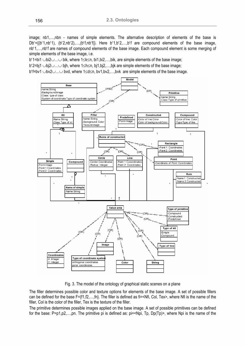
2.3. Ontologies
156
image; nb1,…,nbn - names of simple elements. The alternative description of elements of the base is Db′=(b′1,nb′1), (b′2,nb′2),…,(b′f,nb′f). Here b′1,b′2,…,b′f are compound elements of the base image, nb′1,…,nb′f are names of compound elements of the base image. Each compound element is some merging of simple elements of the base image, i.e. b′1=bi1 ∪bi2∪…∪ bik, where 1≤k≤n, bi1,bi2,…,bik, are simple elements of the base image; b′2=bj1 ∪bj2∪…∪ bjh, where 1≤h≤n, bj1,bj2,…,bjk are simple elements of the base image; b′f=bv1 ∪bv2∪…∪ bvd, where 1≤d≤n, bv1,bv2,…,bvk are simple elements of the base image.
Fig. 3. The model of the ontology of graphical static scenes on a plane
The filler determines possible color and texture options for elements of the base image. A set of possible fillers can be defined for the base F=f1,f2,…,fn. The filler is defined as fi=<Nfi, Cоl, Tex>, where Nfi is the name of the filler, Col is the color of the filler, Tex is the texture of the filler. The primitive determines possible images applied on the base image. A set of possible primitives can be defined for the base: P=p1,p2,…,pn. The primitive pi is defined as: pi=<Npi, Tp, Dp(Tp)>, where Npi is the name of the

KDS 2005 Section 2: Data Mining and Knowledge Discovery
157
primitive, Tp is the type of the primitive, Dp(Tp) is the description of the primitive. The type of any primitive can be defined as Tr is predefined, Tb is constructed, Tc is compound. By the predefined primitive is meant a primitive whose image is known. The description Dp(Tr) of the predefined primitive is Dp(Tr)= < Ip>, where Ip is the image of the primitive. The constructed primitive it defined by a form, a color of a line and a background. Hence it has the following description: Dp(Tb)=< F, R(F), Сl, Cb>, where F is the form of the primitive, R(F) is the rule for construction of the primitive of a specified form, Сl is the color of the line, Сb is the color of the background. The following forms of a primitive are defined: a circle, a point, a line and a rectangle. For each form, it is necessary to define rules of its construction. The rule of a circle construction is defined by the circle center coordinates and radius: R(circle) =<(х,y), r>; the point is defined by the coordinates: R(point) =<(х,y) >; the line is defined by coordinates of two points: R(line) =<(х1,y1), (х2,y2)>; a rectangle is defined by coordinates of two points, its top left and lower right vertexes: R(rectangle) =<(х1,y1), (х2,y2)> . The compound primitive is a set of constructed primitives, connected by themselves by lines of a certain color and type: Dp(Tc)=< (Npi, Npj), (Npj Npk),…, (Npn Npv), Cl, Lt>. To describe the compound primitive it is necessary to determine a set of pairs of constructed primitive names (Npi, Npj), that must be connected by lines of a certain color Cl and type Lt.
The Design Process of Dialog in the Form of Graphical Static Scenes
The design process of dialog in the form of graphical static scenes is carried out in two phases. At the first phase, it is necessary for the interface developer to correlate elements the OGSS with the information, specific for a certain domain. In this way, the developer defines a base, i.e. its image, name (a term of the domain), as well as names and images of base components. Further, with the same editor the developer determines fillers and/or primitives by specifying their possible properties. At the second phase the developer forms the design of the interface, namely, specifies location of the base, primitives, fillers and additional elements of the graphical user interface determined by the OGUI. The input data dialog of the user with the applied program consists in composing the graphic static scenes. Fig. 4 shows examples of graphical static scenes. According to the specification of the OGSS for a certain domain, the interface recognizes a graphic scene and transfers values of the output data to the applied program in the format assigned by the developer. Then the interface generates graphical scenes based on computation results of the applied program in conformity with the same description.
Discussion Development of the user interface combining various types of dialog (verbal and graphical) is a topical problem. No less important, as noted above, is the problem of reducing the cost of development and simplifying maintenance of the user interface. In the paper, we have considered how the proposed technology of development allows the specified problems to be solved. First, the interface is automatically generated based on the declarative description of its model. Second, information for each component of the model is formed on the basis of the ontology model offered to the developer. Third, the interface developer can generate various types of dialogues according to requirements of users (verbal and/or graphical on the basis of the OGUI and the OGSS.
Fig. 4 Examples of graphical static scenes for heat supply and medicine domains.

2.3. Ontologies
158
Fourth, information transmitted to the applied program and back (the input/output data) does not depend on the form of its representation to the user and is formed based on the domain model. Thus, modification of the dialog does not require any modification of other interface components.
Acknowledgements
The research was supported by the Far Eastern Branch of Russian Academy of Science, the grants 05-02-01-027, 05-01-01-119.
Bibliography
1. Sommerville I. Software engineering. Addison-Wesley Publishing company,1997. 2. Gribova V., Kleshchev A. From an ontology-oriented approach conception to user interface development International
//Journal Information theories & applications. 2003. vol. 10, num.1, p. 87-94 3. Da Silva P.P., Griffiths T. and Paton N.W., Generating User Interface Code in a Model-Based User Interface
Development Environment, Proc. Advanced Visual Interfaces, V. di Gesu, et al. (eds), ACM Press, 2000. 4. http://interface.es.dvo.ru/ontology.htm 5. The unified modelling language. http://www.uml.org/
Author's Information Gribova Valeriya –Ph.D. Senior Researcher of the Expert System Department, Institute for Automation & Control Processes, Far Eastern Branch of the Russian Academy of the Sciences: Vladivostok, +7 (4323) 314001 [email protected], http://www.iacp.dvo.ru/es.
ОНТОЛОГИИ КАК ПЕРСПЕКТИВНОЕ НАПРАВЛЕНИЕ ИНТЕЛЛЕКТУАЛИЗАЦИИ ПОИСКА ИНФОРМАЦИИ В МУЛЬТИАГЕНТНЫХ СИСТЕМАХ Е-КОММЕРЦИИ
Анатолий Я.Гладун, Юлия В.Рогушина Аннотация. Предлагается использовать онтологическое представление знаний об интересах покупателя в процессе е-коммерции. Это повышает эффективность поиска наиболее продавцов, наиболее подходящих покупателям, мультиагентными системами. Реализован алгоритм сравнения онтологий покупателей с онтологиями электронных магазинов (таксономий) и мультиагентная система электронной коммерции, использующая онтологии для поиска информации в распределенной среде.
Ключевые слова: онтология, е-коммерция, мультиагентная система.
Введение
Сегодня мы являемся свидетелями и участниками эволюции постиндустриального общества в общество, называемое информационным. В информационном обществе приоритетным направлением является создание и эффективное использование знаний и информационных ресурсов. Колоссальные перспективы развития рынка товаров и услуг в сети Интернет впечатляют даже специалистов - только за последние месяцы прошлого года торговый оборот сети возрос в несколько раз. Стремительный технический прогресс в этой области дает мощный импульс глобализации мировой экономики и делает все более привлекательным объектом инвестиций новые информационные технологии, направленные на развитие электронной коммерции (е-коммерции).

KDS 2005 Section 2: Data Mining and Knowledge Discovery
159
Однако происходящие изменения приводят к возникновению ряда новых проблем. Поистине огромный объем предложений, широкое разнообразие товаров и услуг, высокая динамика изменений рынка – все это приводит к резкому возрастанию сложности и трудоемкости работы как продавцов, так и покупателей в сети, отнимает их время и тем самым повышает стоимость данных услуг. Нужна кардинальная смена самой концепции обработки информации в сети Интернет, которая бы позволила более содержательно отвечать запросам клиентов, более оперативно реагировать на изменяющиеся требования и гибко адаптироваться к условиям рынка. Вхождение Украины в мировое информационное пространство требует решения многоаспектной проблемы автоматизации современных бизнес–приложений. Под электронным бизнесом понимают все формы электронной бизнес-деятельности, такие как е-коммерция, е-консалтинг, е-издательство и т. п. Е-коммерция является частным случаем электронного бизнеса. Под е-коммерцией понимают различные формы торговли товарами и услугами посредством использования электронных средств, в том числе и Интернета. При этом заказ товаров осуществляется через телекоммуникации, а расчеты между покупателем и продавцом - при помощи электронных средств платежа [1]. Улучшение эффективности выполнения задач е-бизнеса требуют дальнейшего развития методов автоматизации бизнес-процессов. Системы е-коммерции должны обеспечивать потребителю доступ к информации о товарах, представленной в электронной форме, и ее быстрый поиск в сетевой среде. Сложность транзакций очень велика из-за динамичности и огромного количества информации, доступной пользователям через Интернет. Индустриальная разработка программного обеспечения для е-коммерции требует создания и использования соответствующих моделей, стандартов, языков и форматов, ориентированных на обработку знаний. Для решения этих задач с успехом применяются агентно-ориентированные технологии, базирующиеся на использовании интеллектуальных программных агентов (ПА).
Системы поддержки е-коммерции
Сейчас для поддержки электронной коммерции разработано много разнообразных программных продуктов разного уровня сложности. Моделирование реальных приложений должно отображать сложность бизнес-процессов реального мира. Представляется очевидным, что необходима интеллектуализация таких средств, чтобы избавить пользователя от необходимости самостоятельно выполнять повторяющиеся действия. В частности, наиболее популярным на сегодняшний день является использование в е-коммерции ПА и мультиагентных систем (МАС). Одна из главных трудностей практического подхода связана с объединением сложных интеллектуальных способностей в мобильных ПА. ПА - это программное обеспечение, обладающее рядом характерных свойств, предназначено для упрощения диалога пользователя со сложным и динамичным информационным окружением. Многие исследователи определяют ПА как программную сущность, которая функционирует продолжительно и автономно в конкретном окружении, часто вместе с другими процессами и ПА [2]. Продолжительность и автономность позволяют ПА гибко и интеллектуально действовать в соответствии с изменениям среды без постоянных указаний или вмешательства пользователя. В идеальном варианте агент, который долгое время функционирует в среде, должен быть способен обучаться на своем опыте. Кроме того, ПА, который сосуществует в среде с другими агентами и процессами, должен быть способен общаться и кооперироваться с ними [3,4]. Мы проанализировали ряд агентов ЭК. PersonaLogic [5] отфильтровывает список товаров, которые удовлетворяют ограничениям пользователя. Firefly выбирает товары через оценки других потребителей. BargainFinder [6] - виртуальный агент покупок, способный оценить цены и их пригодность для пользователя. Он представляет вопрос потребителя параллельно группе on-line продавцов, заполняя форму на каждом сайте. Kasbah [7] - on-line МАС для транзакций типа "потребитель-потребителю". Пользователь, желающий продавать или покупать товары, создает агента, задает этому некоторое стратегическое направление и отсылает его к централизованному агентному рынку. Агенты Kasbah проактивно разыскивают потенциальных покупателей или продавцов и ведут переговоры с ними от имени их создателя. Tete-a-Tete [8] используется для посредничества и переговоров, обеспечивая потребностям и продавцов, и покупателей.

2.3. Ontologies
160
При поиске продукта покупатель выбирает набор характеристик товара, которые представляют для него интерес. Если не найден товар, полностью удовлетворяющий всем требованиям, тогда либо появляется сообщение, что результат не найден, либо список товаров, частично удовлетворяющих запросу. При этом принципы ранжирования результатов поиска часто непонятны пользователю. Заказчик не получает ни четкого обзора результатов, ни предложений для дальнейшего исследования. Идеальной была бы ситуация, в которой покупателю предлагались бы альтернативы, наиболее близкие к его потребностям. Но для этого система должна обрабатывать знания о конкретном заказчике. К сожалению, большинства существующих систем е-коммерции не обеспечивают общий язык взаимодействия, стандартизированное описание домена, адаптируемость, способность к обучению, персонализацию. Агенты е-коммерции, созданные различными разработчиками, не способны взаимодействовать друг с другом. Кроме того, использование многих терминов и выражений крайне неоднозначно и в значительной мере зависит от той предметной области (ПрО), которая интересует пользователя.
Постановка задачи ПА, которые ищут информацию только по ключевым словам, не имеют прикладных знаний о ПрО, которая интересует пользователя, а самостоятельно извлекать эти знания могут только после продолжительной работы и поэтому дают крайне нерелевантные результаты. Поэтому необходимо найти формализованные средства представления таких знаний и разработать алгоритмы, позволяющие агентам эффективно использовать их в поиске товаров и услуг мультиагентными системами е-коммерции. В связи с этим мы предлагаем использовать описания ПрО, которые интересуют конкретного пользователя, представленные в виде онтологий - средство построения распределенных и неоднородных систем баз знаний. Это позволяет избежать разногласий в использовании терминологии и помочь агентам установить правильные соответствия между предложениями продавцов и потребностями покупателей. При этом предполагается, что продавцы также предоставляют пользователям знания о предлагаемых товарах, представленные в виде онтологий.
Онтологическое представление знаний Онтология - это знания, формально представленные на базы концептуализации, которая предполагает описание множества объектов и понятий, связей между ними. Формально онтология состоит из терминов, организованных в таксономию, их определений и атрибутов, а также связанных с ними аксиом и правил вывода. Часто набор предположений, которые составляют онтологию, имеет форму логической теории первого порядка, где термины словаря являются именами унарных и бинарных предикатов, которые называют соответственно концептами и отношениями. В простейшем случае онтология описывает только иерархию концептов, связанных отношениями категоризации. В более сложных случаях к ней добавляются подходящие аксиомы для отображения других отношений между концептами и для того, чтобы ограничить их интерпретацию. Онтология - это база знаний, описывающая факты, которые предполагаются всегда истинными в рамках определенного сообщества на основе общепринятого значения словаря, который используется. Формальная модель онтологии О - упорядоченная тройка вида: O=<X, R, F>, где Х - конечное множество концептов предметной области, которое представляет онтология O; R - конечное множество отношений между концептами заданной предметной области; F - конечное множество функций интерпретации, заданных на концептах и/или отношениях онтологии O [9].
Создание онтологий покупателей
На сегодняшний день разработано довольно много языков представления онтологий (например, DAML-OIL, OWL [10]) и свободно распространяемых инструментальных средств их создания (например, Protégé [11], OntoEdit [12]). Большие онтологии, такие как CYC, создаются на основе абстрактного и очень общего описания понятий предметной области и связей между ними. Основная цель проекта CYC - раз и навсегда построить базу
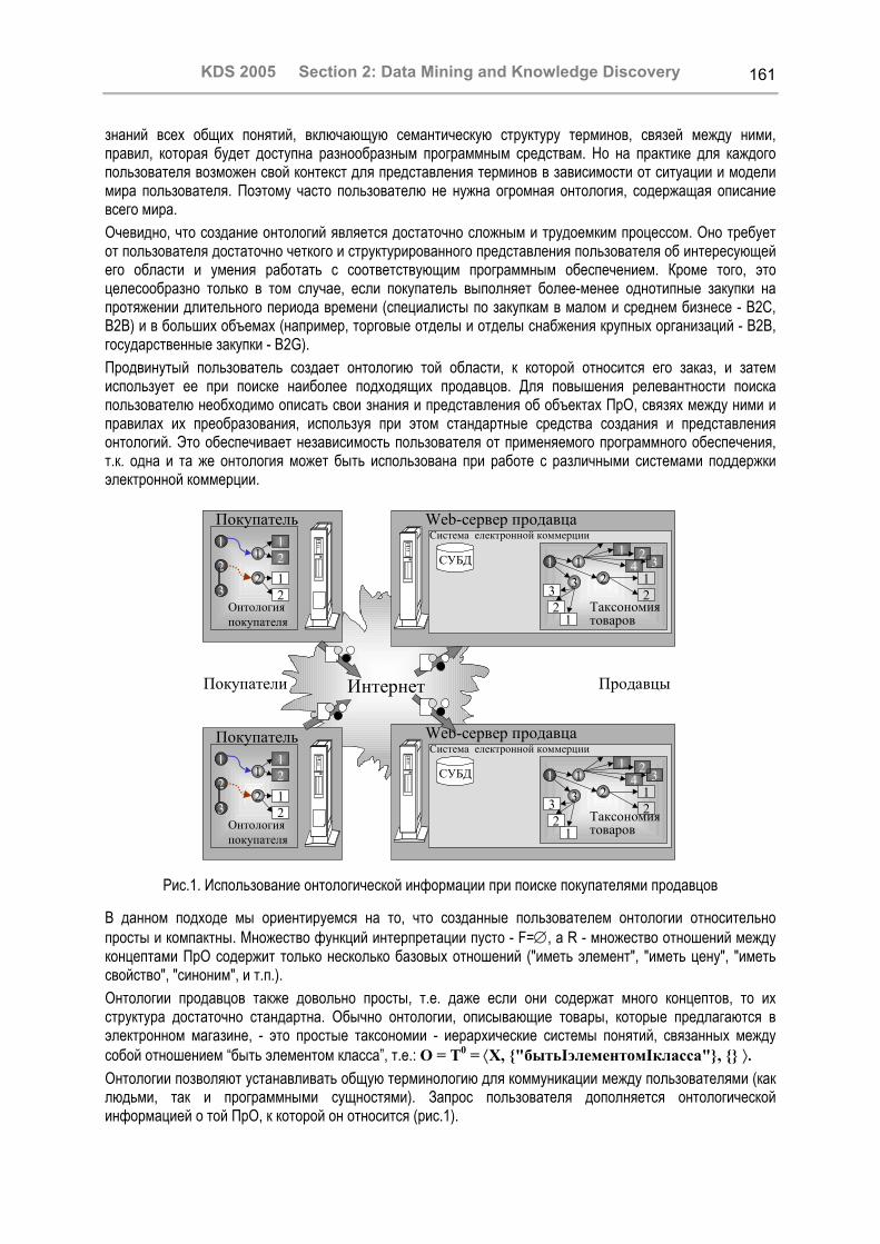
KDS 2005 Section 2: Data Mining and Knowledge Discovery
161
знаний всех общих понятий, включающую семантическую структуру терминов, связей между ними, правил, которая будет доступна разнообразным программным средствам. Но на практике для каждого пользователя возможен свой контекст для представления терминов в зависимости от ситуации и модели мира пользователя. Поэтому часто пользователю не нужна огромная онтология, содержащая описание всего мира. Очевидно, что создание онтологий является достаточно сложным и трудоемким процессом. Оно требует от пользователя достаточно четкого и структурированного представления пользователя об интересующей его области и умения работать с соответствующим программным обеспечением. Кроме того, это целесообразно только в том случае, если покупатель выполняет более-менее однотипные закупки на протяжении длительного периода времени (специалисты по закупкам в малом и среднем бизнесе - B2C, B2B) и в больших объемах (например, торговые отделы и отделы снабжения крупных организаций - В2В, государственные закупки - В2G). Продвинутый пользователь создает онтологию той области, к которой относится его заказ, и затем использует ее при поиске наиболее подходящих продавцов. Для повышения релевантности поиска пользователю необходимо описать свои знания и представления об объектах ПрО, связях между ними и правилах их преобразования, используя при этом стандартные средства создания и представления онтологий. Это обеспечивает независимость пользователя от применяемого программного обеспечения, т.к. одна и та же онтология может быть использована при работе с различными системами поддержки электронной коммерции.
Web-сервер продавцаСистема електронной коммерции
СУБД 1 13
3
12
3
421
2 12
Таксономиятоваров
1
2
3
1
2
1212
Онтологияпокупателя
Покупатель
1
2
3
1
2
1212
Онтологияпокупателя
Покупатель Web-сервер продавцаСистема електронной коммерции
СУБД 1 13
3
12
3
421
2 12Таксономия
товаров
Покупатели ПродавцыИнтернет
Рис.1. Использование онтологической информации при поиске покупателями продавцов
В данном подходе мы ориентируемся на то, что созданные пользователем онтологии относительно просты и компактны. Множество функций интерпретации пусто - F=∅, а R - множество отношений между концептами ПрО содержит только несколько базовых отношений ("иметь элемент", "иметь цену", "иметь свойство", "синоним", и т.п.). Онтологии продавцов также довольно просты, т.е. даже если они содержат много концептов, то их структура достаточно стандартна. Обычно онтологии, описывающие товары, которые предлагаются в электронном магазине, - это простые таксономии - иерархические системы понятий, связанных между собой отношением “быть элементом класса”, т.е.: O = T0 = ⟨X, "бытьІэлементомІкласса", ⟩. Онтологии позволяют устанавливать общую терминологию для коммуникации между пользователями (как людьми, так и программными сущностями). Запрос пользователя дополняется онтологической информацией о той ПрО, к которой он относится (рис.1).

2.3. Ontologies
162
Сравнение онтологий покупателей и продавцов Мы использовали онтологическое представление знаний в разрабатываемой МАС е-коммерции для персонификации агентов покупателей и агентов продавцов: преимущества предоставлялись тем продавцам, в онтологиях которых было больше терминов из онтологий покупателей. Сопоставление онтологий требует разнообразных методов, методологий и технологий, которые необходимы для эффективного использования в выполнении различных заданий онтологий, полученных из различных источников. Каждая из онтологий ПрО может охватывать определенные аспекты знания и может использовать различную терминологию. Должны быть созданы специальные онтологии отображения для связи различных терминологий и стилей моделирования, использованных в этой специфической для домена онтологии. Сегодня существуют программные системы, предназначенные для этого. Например, в проекте Sesame обеспечивается сравнение версий онтологий, представленных в формате RDF, и анализ этих изменений. Но такое программное обеспечение слишком сложно для пользователей, не специализирующихся в ИТ.
1
2
3
1
2
1212
Онтологияпокупателя
1
1
3
3
123
4
21
212
Онтологияпродавца
Данный элементприсутствует в
онтологиипродавца
Данный элементприсутствует в
онтологиипокупателя
БЗ
Онтологииимеют общий
элемент
Рис.2. Предварительный шаг сравнения онтологий – поиск одинаковых элементов.
Мы предлагаем сравнивать онтологии следующим образом: для пары онтологий О1 и О2 строится оценочная функция f(O1, O2), которая определяет их меру близости. При этом учитываются следующие факторы: − вхождение одного и того же термина в обе онтологии; − то, что два термина находятся в разных онтологиях в одном и том же отношении; − то, что два термина находятся в разных онтологиях в отношениях одного типа или разных
(например, в иерархическом отношении и отношении синонимии); − существуют ли вообще любые отношения (прямые или опосредствованные) между одними и теми же
терминами. На предварительном этапе сравнения онтологий (рис.2) формируется множество элементов – концептов ПрО , которые входят в обе онтологии.
Затем проверяются попарно все отношения, в которых состоят эти элементы. Пользователь должен определить для каждого используемого им отношения, к какой группе оно относится. В онтологии продавца такая проблема не возникает в связи с тем, что используется единственное иерархическое отношение. Коэффициенты, определяющие вес различных факторов, зависят от специфики ПрО и определяются пользователем. В наиболее простом случае используется только первый фактор.
21 OO XXY ∩=

KDS 2005 Section 2: Data Mining and Knowledge Discovery
163
Программная реализация
В системе е-коммерции выделяются три взаимосвязанные подсистемы: торговля, управление диалогом и поиск товаров на основе онтологий. В торговой подсистеме могут быть агенты товаров и заказов, а также агенты продавцов и покупателей, склада, поставщиков и т.д. Агенты товаров и заказов ведут переговоры со стратегиями скидок для постоянных покупателей, скидок за оптовую покупку, скидок по состоянию конкурентов, скидок по затовариванию склада и др. При этом несколько агентов покупателей (потенциальных конкурентов) могут объединить свои заказы для получения большей скидки, т.е. перейти от конкуренции к кооперации. В подсистеме же управления диалога нужно создать систему выдачи результатов переговоров агентов. Подсистема онтологии обеспечивает быстрый поиск в распределенной среде релевантного товара для покупателя.
Рис. 3 Окно ведения переговоров между торговцем и покупателем через посредника
На основе анализа существующих МАС е-коммерции [5-9] мы сформулировали требования к программной реализации: 1. Обеспечение переносимости кода на различные платформы (UNIX, LINUX, Windows). 2. Доступность других платформ в сети. Это требование является продолжением предыдущего.
Мобильные агенты должны осуществлять свою работу в гетерогенной компьютерной среде. 3. Поддержка сетевого взаимодействия. Помимо операций, непосредственно связанных с
перемещением между агентскими серверами, агент должен обладать средствами для коммуникации с другими агентами и доступа к удаленным ресурсам. Поэтому поддержка сетевых услуг должна включать в себя широкий спектр возможностей (служба имен, RPC, OLE, CORBA, RMI и т.д.).
4. Многопоточная обработка. Для реализации одновременного выполнения нескольких действий агентская система должна включать в себя поддержку параллельного выполнения функций агента и поддержку средств синхронизации.
5. Безопасность. Мобильные агенты, приходящие из сети, могут содержать потенциально опасный, вредоносный код. Поэтому система должна поддерживать средства безопасности, достаточные для ее нормальной работы.
Для разработки логической модели МАС использовался язык UML. Структура МАС включает: модуль интерфейса; модуль функций для взаимодействия с пользователем (обработчик событий); главный модуль МАС – модуль координации и управления (в соответствии с поставленной задачей) и модуль

2.3. Ontologies
164
онтологий для работы с данными (сортировка, фильтрация, поиск и т.д.); модуль возврата результатов пользователю (в виде log-файла - сообщений на интерфейс пользователя). На основе Java разработан FacilitatorAgent (агент–посредник), который управляет рынком, а также агенты BuyerAgents (агенты–покупатели) и SellerAgents (агенты–продавцы), используемые для взаимодействия внутри этого рынка. Все эти интеллектуальные агенты получены из базового класса CIAgent, который детально описан в [14]. Агенты клиента и продавца различаются, прежде всего, сложностью их стратегий переговоров. Переговоры начинаются с простой логики (в терминах if-then-else), а затем переходят к методам формирования правил, которые базируются на приобретенных фактах. Язык KQML конкретизирует формат и содержание взаимодействий между продавцом и покупателем. Процедура BuySellMessages описывает переговоры между продавцом и покупателем в процессе сделки на рынке. Покупатель и продавец никогда не общаются непосредственно, а используют для этого FacilitatorAgent (которого иногда называют агентом брокера) как посредника в переговорах о купле-продаже. Менеджер коммуникаций (BaySelMessage) содержит в себе сообщения, которые должны быть посланы другим агентам, представленные на языке коммуникаций с примитивами на языке KQML: обратиться с просьбой, принять, отвергнуть, изменить, предложить, проинформировать, запросить данные, отказаться и подтвердить. На рис.3 представлено окно МАС, предназначенное для ведения переговоров между торговцем и покупателем в процессе процедуры купли-продажи.
Заключение Представляется целесообразным использовать онтологическое представление знаний в электронной коммерции для автоматизации установления общего словаря для покупателей и продавцов. Применение стандартных форматов для представления онтологий обеспечивает их интероперабельность и возможность их повторного использования для решения других задач. Предложенный в статье подход значительно повысит релевантность поиска и позволит найти наиболее выгодные и соответствующие потребностям пользователя предложения продавцов. Кроме того, это стимулирует у продавцов создание описаний их товаров на семантическом уровне, что само по себе - еще один шаг по преобразованию Интернет в глобальную распределенную БЗ. Реализован алгоритм сравнения онтологий покупателей с онтологиями электронных магазинов (таксономий). Разработана МАС для е-коммерции, использующая онтологии для поиска информации в распределенной среде. Модуль принятия решения в МАС построен с использованием теории нечетких множеств (сочетание числового и лингвистического подходов). Алгоритм принятия решения позволил выделить три группы агентов в системе по уровню их “интеллектуальности”. Описан протокол переговоров сбыта, который предоставляет более широкие возможности контроля над процессом продажи. Как и в других областях, в е-коммерции повышение эффективности непосредственно связано с использованием знаний и их интероперабельностью. Представленная МАС может использоваться как для моделирования ситуаций, связанных с рынком, так и для разработки готового программного продукта не только для е-коммерции, но и для других бизнес-приложений, например, для электронного документооборота в корпоративных системах.
Перспективы дальнейших исследований Упорядочение онтологий очень важно в контексте Semantic Web. Semantic Web предоставит нам большое количество свободно доступных онтологий, специфических для разных доменов. Чтобы сформировать реальную семантическую сеть, которая позволит компьютерам комбинировать и выводить неявное знание, эти отдельные онтологии должны быть упорядочены и связаны. Формирование онтологии - трудная задача, которая требует углубленного знания домена и, в большинстве случаев, специальных навыков из области инжененерии знаний. Для того, чтобы облегчить процесс конструирования онтологии, необходимо разрабатывать методологии, которые позволят автоматизировать извлечение структурированного знаний пользователей об области их интересов. Еще одни важным направлением для дальнейших исследований представляется разработка более выразительных средств представления онтологий – как языков, так и программного обеспечения.

KDS 2005 Section 2: Data Mining and Knowledge Discovery
165
Список литературы 1. Gladun A., Rogushina J. Multiagent Ontology-Based Intelligent System Of E-Commerce // Proceedings of Int.Conf.
TPSD`2004, Kiev. - P.55-58. 2. Rao A.S., Georgeff M.P. Modelling rational agents within a BDI-architecture. In R. Pikes and E. Sandewall, eds.. Proc.
of Knowledge Representation and Reasoning (KR&R-91), Morgan Kaufmann Publishers: San Mateo, CA, April 1991. - P. 473-484.
3. Bratman M. E., Pollack M. E. Toward an architecture for resource-bounded agents. Technical Report CSLI-87-104, Center for the Studv of Language and Information, SRI and Stanford University, August 1987.
4. Cohen P.R., Levesque H.J. Intention is choice with commirment. Artificial Intelligence. N 42. 1990. - P.213-261. 5. PersonaLogic. - http://www.personalogic.com. 6. Firefly.- http://www.firefly.com. 7. BargainFinder. - http://bf.cstar.ac.com/bf. 8. Kasbah. - https://kasbah.media.mit.edu. 9. Tete-a-Tete. - (http://ecommerce.media.mit.edu/tete-atete. 10. OWL. Web Ontology Language. W3C. - http://www.w3c.org/TR/owl-features/. 11. Protégé. - http://protege.stanford.edu/ontologies/ ontologyOfScience. 12. OntoEditTM Datasheet. - http://www.ontoprise.de/customercenter/index.html. 13. Гаврилова Т.А., Хорошевский В.Ф. Базы знаний интеллектуальных систем. - Спб.: Питер, 2001. 14. Gladun A., Gritsenko V. Multi-Agent System Model For E-Business And Its Computer Software Implementation
Technology // Problems of Programming, 2004, 2-3, P. 510-520.
Информация об авторах
Гладун Анатолий Ясонович – к.т.н., с.н.с. Международного научно-учебного центра информационных технологий и систем НАНУ и МОН Украины Адрес для переписки – 01033, Киев, пр. Ак.Глушкова, 40, тел.(044)266-63-44, E-mail: [email protected] Рогушина Юлия Витальевна, к. ф.-м.н., с.н.с. Института программных систем НАНУ Адрес для переписки – 01033, Киев, пр. Ак.Глушкова, 40, тел.(044)268-46-98, E-mail: [email protected]
IMPLEMENTING SIMULATION MODULES AS GENERIC COMPONENTS
Anton Kolotaev Abstract: In this paper generic programming techniques applicability to build simulation models library is discussed. Policy-based design is proposed for implementation simple simulation modules.
Keywords: generic programming, library design, discrete-event simulation, policy-based design.
Introduction
Modular decomposition of a simulation model into a set of interacting components is generally accepted method and has a long history. Advantages of modular approach are well known. First of all, it allows reflecting the structure of a model being simulated into the simulation program code that undoubtedly helps in the program comprehension and makes its maintenance easier. Secondly, the approach gives opportunity for using a module as a building block for many simulations that is for module reuse. It greatly reduces new simulation models development and debugging costs. The more complex a model constructed the more evident modular approach advantages become. One of the most widely used languages to develop simulations of large and complex systems (such as telecommunication systems) is C++. This is due to flexibility and efficiency of the language.

2.3. Ontologies
166
One who develops a simulation program in C++ can use all power of the general-purpose programming language with its highly developed machinery to build abstractions that proves to be very useful when dealing with complex data structures and non-trivial algorithms that arise in complex systems simulations. C++ programming language allows creating highly expressive programs which executables are efficient as analogous programs written in lower level languages. When using C++ one can minimize penalty due to introducing abstractions and writing the program on a higher level that is to eliminate abstraction penalty. Execution slow down is acceptable in case it takes several seconds and efficiency could be sacrificed to easier model development. Simulations of large telecommunication systems may take hours of execution and a tool that introduces no abstraction penalty is very relevant to simulating large systems. General-purpose languages (including C++) don’t offer any ready components to build simulation programs. A platform providing simulation modules coordination have to implemented as well as auxiliary components that are often used when building simulations (for instance, various random number generators with certain distribution laws). Simulation libraries provide frameworks and auxiliary components to build simulations. Some libraries are delivered together with simulation model libraries for certain domains, e.g. ns-2 simulator [1] is delivered with large number components that simulate network routers and links. Several libraries come with tools that help in conducting simulation experiments. For example, OMNeT++ [2] contains graphical module editor GNED, running the simulation environment Tkenv, Plove for analyzing simulation results etc. To design a good library is more challenging task than to design a single application. One of the hardest tasks is to design a library so that it could evolve without making to modify a code that uses the library. A simulation model library should possess provide interoperable, customizable components. Invalid component parameter combinations as well as composing components which interaction is not permitted should be detected as soon as possible (it is advisable to detect and localize such situations before simulation execution). Simulation model library should be open for interaction with libraries in other domains (e.g. one may need graph library to deal with network topology; modern random number generators are made as standalone libraries, e.g. Boost.Random [3]). Extensibility is an important feature of a simulation library. The library user has to be given an opportunity to create own simulation model components easily. Such components should be interoperable as native for the library ones. The main method to achieve these qualities is abstracting a component that could describe in simplified form as a factoring any non-relevant points as the component’s parameters. Binding with the parameters various values, we can achieve different behaviors of the component. In object-oriented languages, the main way of such parameterization is applying dynamic polymorphism, which is often presented by virtual functions language feature. Unfortunately, such parameterization by OOP methods can be performed only to a certain extent, when virtual function usage overhead becomes unacceptable high. The main impact on performance lies in compilers’ inability to inline the virtual function body into the invocation point that prohibits many optimizations around the invocation point. In addition to the loss of performance type safety may be damaged (non-typed containers in Java and C# is illustrating example) and many checks that could have been performed at compile-time cannot be performed until run-time. Bounded dynamic polymorphism requires classes which to be used as parameters to be inherited from some base classes (so called intrusive, or invasive polymorphism) that reduces the components’ adaptability (we may mention primitive types boxing/unboxing in Java and C#). The issues stated could be solved if parameters’ binding is made at compile-time, so called static polymorphism, which is supported in C++ language by very powerful template machinery. Since language means providing static polymorphism differ from ones providing dynamic polymorphism by abstractions construction properties, design with static polymorphism requires following to principles that differ from OOP principles. Such principles are studied in the field of generic programming. According to [4], Generic programming is a sub-discipline of computer science that deals with finding abstract representations of efficient algorithms, data structures, and other software concepts, and with their systematic organization. The goal of generic programming is to express algorithms and data structures in a broadly adaptable, interoperable form that allows their direct use in software construction. There are some domains for which generic programming libraries are developed and widely used: linear data structures (dynamic array, list, deque, balanced tree) and algorithms on them – STL, algorithms and data

KDS 2005 Section 2: Data Mining and Knowledge Discovery
167
structures for computational geometry – CGAL (Computational Geometry Algorithm Library) [5], graphs – BGL (Boost Graph Library), matrices – MTL, GMCL (Generative Matrix Computational Library), arrays for numerical computing – blitz++, iterative numeric methods – ITL++ etc. OMNeT++ library design makes clear-cut distinction between simple and compound modules in simulation models library. Simple modules contain the algorithms in the model. All model behaviors are a composition of simple modules’ behavior. Compound modules govern such composition. They are composed of other modules (it doesn’t matter whether they are simple or compound) and are to bind aggregated modules parameters and input and output ports. The valuable idea is that all behavioral aspects of a model are contained in simple modules while all combinatorial aspects are contained in compound modules. In this paper generic programming techniques to implement, simple modules are discussed. For this purpose, we will consider applicability of policy-based design described in [6] in depth. We are aimed to achieve the following design goals:
1. Simple module should be as stable to changes in simulation library architecture as possible. 2. Models composed from library modules should not be less effective in terms of execution time and
memory consumed than monolithic models. 3. Simulation modules should be very customizable and allow every reasonable customization.
The techniques to be described are used telecommunication systems simulation library Tksym developed by the author for comparative analysis of various routing algorithms.
Language Features to Capture Variability
Firstly, we should select appropriate language mechanism to capture variability of simple modules. For throughout discussion of concepts about variability in software the reader is referred to [4]. Object-oriented programming offers two design patterns to capture behavioral variability namely Strategy and Template Method design patterns [7]. Let’s assume that we have component C with variable features f1, …, fN. When using Strategy design pattern each feature fi will be presented in C by a pointer to abstract base class F1. During run-time, the user binds the pointer with concrete strategy object. When N is quite big there is memory overhead to store N pointers. On the other hand, the user needs not to define new classes he/she only configures at run-time the component. When using Template Method class C has virtual functions F1, FN for each variable feature. The users bind the component with certain set of concrete features by defining a class that inherits from C and implements member functions F1, FN. In this case, memory overhead is fixed – storing virtual functions table pointer per class object. User has to implement a new class each time he/she needs to instantiate C with new feature combination. Without templates, it is very painful task. When we move from virtual functions to class templates more variability schemes arise. We may parameterize C by N template parameters F1, FN. There are several strategies to access from C to concrete features. Firstly, concrete features may be implemented as static member functions in Fi. There is no time or memory overhead but this approach doesn’t allow associating some state with concrete features. Alternative approach is to aggregate in C concrete feature objects of type Fi. Features may be accessed as ordinary member functions. Such approach has the following disadvantage: some memory is needed to store each object even it has zero size. The disadvantage can be avoided by inheriting class C from features F1, FN. If the compiler used supports Empty Base Class Optimization (EBCO), empty base classes will contribute no memory overhead to class C. This resembles Strategy design pattern except it is done at compile-time. Instead of parametrizing C by N parameters we may aggregate them as nested types to a single type which will be the parameter of C. We may parameterize C by a class derived from it. It is called curiously recurring template. Features are accessed from C by casting this pointer to derived class. It is very helpful technique in many cases. Suppose there are set of elementary functionalities E = e1, …, eN and there are set of concrete classes C = C1, …, CM and a concrete class Fi has functionality obtained by combining some subset of elementary features. An elementary feature embedded in concrete component might want to have access to other elementary features that constitutes the component. Curiously, recurring template trick is elegant solution to this design problem.

2.3. Ontologies
168
Unfortunately, it is not advisable to apply it to simulation module construction (it was the main method for combining elementary functionality in earlier versions of Tksym). Elementary functionality assume existence certain member functions in derived class that restricts the method scalability (Function member name collisions may appear as the concrete component is getting more complex and consisting more and more base classes. To solve such collisions the user has to introduce complicated class hierarchy that greatly reduces the program understanding). Policy-based design is chosen to implement simple modules in Tksym.
Implementing Simple Server Module in Policy-based Design
Let’s consider policy-based implementation of simple server s that behaves according the following algorithm. When an entity e arrives into s, check that s is free is performed. If s is busy then e is stored in a queue q associated with s. If s is in idle state, s starts processing e for some time t(e). After the processing has complete, e is to be sent further and s asks q is there are any entities to process. If q contains such an entity it is extracted from q and is sent for processing to s. If q is empty s returns to idle state.
template < class Base, class World, class Queue, class ProcessingTime, class Sink, class Events > struct Server : Base, World, Queue, ProcessingTime, Sink, Events typedef Base::Entity Entity;
using Queue::queue; using Events::events;
// input port of the module where it receives messages from other modules void process (Entity e) if (being_sent_) // if the server in busy state queue()->push(e); // store e in queue else // else startProcessing(e); // start processing it
// external clients may want to know state of the server Entity const & beingSent() const return beingSent_; private:
void startProcessing(Entity e) // evaluate time t to process e // and schedule to call “release” after t seconds World::schedule(ProcessingTime::get(e), boost::bind(&ResourceEx::release,this)); // go to busy state being_sent_ = e;
// notify event listeners processing of e has started events()->OnStartProcessing(e);
void release() // place entity has been processed to output port Sink::process(being_sent_);
// notify event listeners that processing of e has finished events()->OnStopProcessing(being_sent_);
// go to idle state being_sent_ = 0;
// if there are any entities to process if (!queue()->empty())

KDS 2005 Section 2: Data Mining and Knowledge Discovery
169
// start processing of the first one startProcessing(queue()->top());
// remove it from the queue queue()->pop();
private: Entity being_sent_; ;
At the first place, It is to be noted that template version of Server requires much less from the component’s parameters than if it were designed with virtual functions. Virtual function usage requires exact matching of the functions’ signatures. Template requires from parameters to have members that have parameters list that can be matched to call arguments (that is broader since it includes, for instance, type conversions). For example, the requirement on parameter Base is to contain inner type Entity. Type Entity must have default constructor, copy constructor and cast operator to a type that can be condition in is-statement. An entity constructed by default designates empty entity and serves to indicate idle state of the server. There are syntactic and semantic requirements. If syntactic requirements are violated a compile-time error is reported. Semantic requirement violation may be detected only at run-time by assertions, pre- and post-conditions checking. Let’s discuss some features of the policy-based design. A component is derived from a set of policies that are template parameters. If policy has several member functions they are composed into single class (see, for example Queue and Events policies). It helps to implement policy classes, which delegate their functionality to other classes. Each of the class parameters can be implemented in different ways. For example, class Server can operate with different queues. They may differ by queuing discipline: simple queues with principles first come – first served (FCFS_QueueHolder) or first come – last served (FCLS_QueueHolder), priority queues for which comparison criteria is to be provided (PriorityQueueHolder).
template <class QueueStorage>
struct QueueHolder
typedef QueueStorage queue_type;
queue_type const & queue() const return queue_;
queue_type & queue() return queue_;
private:
queue_type queue_;
;
template <class Entity>
struct FCFS_QueueHolder : QueueHolder <std::queue<Entity> >
;
template <class Enity>
struct FCLS_QueueHolder : QueueHolder <std::stack<Entity> >
;
template <class Entity, class ComparisionCriteria>
struct PriorityQueueHolder :
QueueHolder<std::priority_queue<Entity, ComparisionCriteria > >
;
Server may use exclusive queue (classes that make use of QueueHolder) or shared queue (QueueInDerived or QueueIndirect).
// We assume that Derived has member function QueueType & getQueue()
// and QueueInDerived is base (perhaps, indirect) for Derived

2.3. Ontologies
170
template <class QueueType, class Derived>
struct QueueInDerived
typedef QueueType queue_type;
queue_type const & queue() const
return static_cast<Derived const *>(this)->getQueue();
queue_type & queue()
return static_cast<Derived *>(this)->getQueue();
;
// accessing a queue placed somewhere else
template <class QueueType, class Holder>
struct QueueIndirect
typedef QueueType queue_type;
void setHolder(Holder * h) holder_ = h;
queue_type const & queue() const return holder_->queue();
queue_type & queue() return holder_->queue();
private:
Holder * holder_;
;
Note, since Queue should expose only queue() method there is no need to implement 4 queue_type members (push, pop, top, empty) in every delegating queue. A queue may have infinite or limited capacity. In case of limited capacity, several strategies are possible when an entity is being inserted into a full queue: to ignore the entity, to replace another entity, to move the entity to special handler. Each of the options can be easily implemented as a strategy class.
Conclusion We have discussed simple module implementation using policy-based design. We have made server class highly customizable without sacrifying its efficiency. We have minimized the module’s dependency from simulation platform (The only call to the simulation kernel is World::schedule with nullary callable entity as second argument). A question that remains open is how to compose together different modules, or in OMNeT++ classification how to create compound modules. It requires some kind of metaprogramming: static metaprogramming in C++ or writing special generator or even dedicated CASE tool that supports generic components description. We suggest that compound modules should be binders – metafunctions that bind several parameters with concrete values leaving the rest ones free. Currently in Tksym is being used manual component configuration that looks very awkward and ways to implement compound elegantly are being searched.
Bibliography [1] The Network Simulator - ns-2. Home page. http://www.isi.edu/nsnam/ns/ [2] OMNeT++ Home page. http://www.omnetpp.org/ [3] Boost Random Number Library Home Page. http://www.boost.org/libs/random/ [4] K. Czarnecki and U. Eisenecker. Generative Programming: Methods, Techniques, and Applications. Addison-Wesley, 1999. [5] Computational Geometry Algorithm Library Home Page. http://www.cgal.org [6] Alexandrescu, A. Modern C++ Design: Generic Programming and Design Patterns Applied, Addison-Wesley Professional,
2001. [7] Gamma E., Helm R., Johnson R., Vlissides J. Design Pattern. Addison-Wesley Professional; 1995.
Author's Information
Kolotaev Anton – SPIIRAS, Ph.D student, Saint-Peterburg, V.O. 13th line, 39, Russia; e-mail: [email protected]

KDS 2005 Section 2: Data Mining and Knowledge Discovery
171
ИСПОЛЬЗОВАНИЕ SEMANTIC WEB ТЕХНОЛОГИЙ ПРИ АННОТИРОВАНИИ ПРОГРАММНЫХ КОМПОНЕНТОВ
Михаил Рощин, Алла Заболеева-Зотова, Валерий Камаев Abstract: В данной статье описывается принципиально новый подход при аннотировании компонентов с использованием логического формализма.
Keywords: Semantic Web, компоненты, моделирование, семантика, логический формализм.
Вступление
Цель нашей исследовательской работы заключается в содействии создания программного обеспечения с использованием заранее созданных компонентов, предоставляя семантически полное описание этих компонентов, совместно с методами и техническими приемами для управления и манипуляции ими, внедряя Semantic Web технологии в так называемую структуру аннотирования (которая является универсальной программной системой, предоставляющей семантическое описание компонентов по открытым гибким и централизованным принципам, адаптированным к стандартам системных решений). При этом структура аннотирования приобретет новые свойства и технические возможности для лучшего решения задач логического вывода (например, проверка на непротиворечивость информации), для автоматизации процессов извлечения знаний на основе содержания описания, для обеспечения автоматизированного поиска и конструировании сложных запросов, а также для реализации механизма получения информации и ее интерпретации с различных точек зрения.
Основная часть
В настоящее время, компоненты и их использование являются ключевой проблемой в области создания программного обеспечения. Системы, основанные на компонентах, легко подаются пониманию, построению, системной разборке, в отличии от монолитных систем. Связующие технологии (middleware), ассоциирующиеся с компонентами (CORBA, COM, JavaBeans, и т.д.), обеспечивают стандартизированные независимые решения для взаимосвязи компонентов, способствуя приближению программного обеспечения к стандартам plug-and-play и лучшему повторному переиспользованию относительно системных решений. Кроме того, эти технологии предлагают такие модели компонентов, которые четко соответствуют решению проблемы развития системы. В результате, переиспользование компонентов приобретает все большую популярность в различных проектах. На ранних этапах переиспользованию компонентов придавалось чрезмерное внимание, но подход был слишком упрощенным. Сейчас, сфера практического применения и схема повторного использования, принятые в области технологии системных решений (с соответствующими средствами и методами поддержки создания ПО), делают повторное использование компонентов и развитие системных решений достаточно эффективным. Проведенный анализ подтверждает, что основой этого успеха является соответствующее описание семантической информации о компоненте (например, функциональные и нефункциональные свойства компонента, его поведение, временные требования и ограничения, необходимое обслуживание и т.п.). Стандартная структура аннотирования является универсальной программной системой, которая позволяет описывать компоненты (создавать аннотации, аннотировать) и интерфейсы, как отдельных компонентов, так и их групп. Аннотации могут быть представлены на протяжении всех фаз жизненных циклов компонентов – от предъявления требований к дизайну и его разработке до маркетинговых шагов и внедрения. Для того, чтобы упростить процесс аннотации и обеспечить адекватность ее содержания, аннотация предоставляется на основе модели. Модель аннотации определяются соответствующей проектной группой. Когда тип описания определен, необходимо определить форму, содержание и семантику понятий, используемых в аннотации. Аннотации используются в развитии области системных

2.3. Ontologies
172
решений, чтобы выделить наиболее подходящих кандидатов среди компонентов для включения их в разрабатываемую системы, а они в свою очередь содержат информацию необходимую для их интегрирования. Аннотации могут также служить средством достижения автоматизированного конфигурирования системы. Параллельно с дискуссиями о повторном использовании программного кода и развитии компонентно-ориентированного подхода, демонстрирующие необходимость семантического описания компонентов, Semantic Web технологии получили свое развитие в Internet. Semantic Web означает ассоциирование семантики с web информацией, которую в свою очередь можно использовать для развития интеллектуального программного обеспечения, собирающего информацию из различных независимых источников в Internet и автоматически интегрирующего эту информацию, несмотря на то, что значение этой информации в зависимости от месторасположения и групп пользователей может быть представлено по разному, что заранее не оговаривается. Основная цель Semantic Web заключается в описании различных специфических областей знаний с помощью онтологий, другими словами получение знаний и характеристика области специфических отношений и правил. Последним стандартом для описания онтологий, предложенным W3C, является язык описания web онтологий OWL (Web Ontology Language), который основан на синтаксисе XML. OWL базируется на логическом формализме Description Logics (Логика Описаний), который предназначен для описания правил, применяемых для различных задач логического вывода. Идея Semantic Web обеспечивает наилучшие результаты, когда речь идет о сравнении и соотнесении информации из различных источников, в отличии от простого поиска по ключевым словам, который теряет всякий смысл там, где объем информации растет экспоненциально. По Semantic Web технологиям доступно большое количество результатов исследований, но до сих пор никто не обращал внимания на особенности и специфические требования по семантическому описанию компонентов для повторного использования. Очевидно, что подходы Semantic Web и желаемые механизмы расширения структуры аннотирования имеют одинаковые задачи. При соответствующем подходе задача заключается в решении проблемы манипуляции аннотациями в структуре аннотирования путем добавления логического формализма для представления знаний (используя синтаксис OWL вместо XML) и механизма онтологий в качестве основы моделирования области знаний. Этот подход обеспечит возможность автоматизированного суждения о свойствах компонентов (анализ, проверка на непротиворечивость, извлечение информации и ее представление в различных формах). В дальнейшем, это обеспечит поиск компонентов (что очень важно для переиспользования компонентов), основанном на механизмах логического вывода, путем сравнения и наложения предварительных и окончательных условий на семантическое описание компонентов. До сих пор отсутствовали какие-либо исследования в области использования технологий Semantic Web для аннотирования компонентов в области систем программного обеспечения. Стандартная структура аннотирования предлагает описание компонентов, основанное на моделях и интерфейсе, с точки зрения сложно описываемых свойств, таких как поведение или нефункциональные свойства, требования. Введение технологии Semantic Web позволит усовершенствовать все характеристики, благодаря механизмам, которые содействуют появлению ряда важных новых свойств. Они включают в себя следующее: а) Систематизация описания области знаний:
• Это позволит разработать онтологии специфических областей знаний, написанных с помощью OWL, предоставляя формальное определение классов, ролей и отношений между ними, и соответствующие аннотации. Это обеспечивает создание иерархической структуры (определение классов с помощью других классов и ролей) и определение свойств ролей (например, симметрия, транзитивность и т.д.).
• Онтологии облегчают определение типов аннотаций и, соответственно, предоставляют лучшую структуризацию содержаний аннотаций и более четкое выражение когнитивных понятий.

KDS 2005 Section 2: Data Mining and Knowledge Discovery
173
б) Автоматизированные процедуры: • Автоматизированная мотивация на основе знаний извлеченных из аннотаций (т.е. свойства
компонентов) для многочисленных целей, в частности для получения адекватного компонента в зависимости от желаемых свойств, которые не поддаются точной спецификации. Это обеспечит отбор компонентов и их наложение или сравнение с выбранной схемой моделирования ПО.
• Автоматизированный поиск компонентов с помощью аннотаций. Подобный поиск необязательно должен быть ограничен одной областью знаний (благодаря способности сравнивать семантику).
• Использование и адаптация уже известных семантических описаний. Это используется для извлечения и реорганизации содержания аннотации, в частности при использовании различных языковых групп (например, язык маркетологов и разработчиков).
в) Логический формализм: • Включение дополнительной информации (например, формальное описание дизайна ПО с
помощью UML) в процесс поиска, основанного на аннотациях. • Обеспечение автоматизированной конфигурации компонентов. • Проверка аннотаций на непротиворечивость. • Трансформация аннотаций из одной области описания в другую.
Все эти новые качества будут содействовать уменьшению стоимости разработки и внедрения программного обеспечения основанного на компонентах.
Заключение
Предлагаемый подход при аннотировании программных компонентов предполагает использование логического формализма, что само собой подразумевает нетривиальные решения проблем логического вывода и выразительности языка описания. В данный момент мы работаем над созданием метамодели на верхнем уровне абстракции и проводим опыты для подтверждения предложенных решений. В частности мы пришли к выводу о необходимости ввода механизма так называемого «проблемно-ориентированного логического вывода», подразумевающего разбиение семантического описания на ролевые группы и использование соответствующих механизмов логического вывода, в зависимости от используемых логических операторов.
Информация об авторах
Рощин Михаил Александрович – аспирант Волгоградского государственного технического университета, [email protected] Заболеева-Зотова Алла Викторовна – доцент кафедры САПР и ПК, Волгоградского государственного технического университета, доктор технических наук, [email protected] Камаев Валерий Анатольевич – заведующий кафедрой САПР и ПК, профессор Волгоградского государственного технического университета, доктор технических наук, [email protected]

2.4. Computer Models of Common Sense Reasoning
174
2.4. Computer Models of Common Sense Reasoning
DIAGARA: AN INCREMENTAL ALGORITHM FOR INFERRING IMPLICATIVE RULES FROM EXAMPLES (PART 1)
Xenia Naidenova Abstract: An approach is proposed for inferring implicative logical rules from examples. The concept of a good diagnostic test for a given set of positive examples lies in the basis of this approach. The process of inferring good diagnostic tests is considered as a process of inductive common sense reasoning. The incremental approach to learning algorithms is implemented in an algorithm DIAGaRa for inferring implicative rules from examples.
Keywords: Incremental and non-incremental learning, learning from examples, machine learning, common sense reasoning, inductive inference, good diagnostic test, lattice theory.
Introduction Our approach to machine learning problems is based on the concept of a good diagnostic (classification) test. This concept has been advanced firstly in the framework of inferring functional and implicative dependencies from relations [Naidenova and Polegaeva, 1986]. But later the fact has been revealed that the task of inferring all good diagnostic tests for a given set of positive and negative examples can be formulated as the search of the best approximation of a given classification on a given set of examples and that it is this task that all well known machine learning problems can be reduced to [Naidenova, 1996]. We have chosen the lattice theory as a model for inferring good diagnostic tests from examples from the very beginning of our work in this direction. We believe that it is the lattice theory that must be the mathematical theory of common sense reasoning. One can come to this conclusion by analyzing both the fundamental work in the psychological theory of intelligence [Piaget, 1959], and the experience of modelling thinking processes in the framework of artificial intelligence. The process of objects’ classification has been considered in [Shreider, 1974] as an algebraic idempotent semi group with the unit element. An algebraic model of classification and pattern recognition based on the lattice theory has been advanced in [Boldyrev, 1974]. A lot of experience has been obtained on the application of algebraic lattices in machine learning: the works of Finn and his disciples [Finn, 1984], [Kuznetsov, 1993], the model of conceptual knowledge of Wille [1992], the works of the French group [Ganascia, 1989]. The following works are devoted to the application of algebraic lattices for extracting classifications, functional dependencies and implications from data: [Demetrovics and Vu, 1993], [Mannila and Räihä, 1992], [Mannila and Räihä, 1994], [Huntala, et al., 1999], [Cosmadakis, et al., 1986], [Naidenova and Polegaeva, 1986], [Megretskaya, 1989], [Naidenova, et al., 1995a], [Naidenova, et al., 1995b], and [Naidenova, 1992]. An advantage of the algebraic lattices approach is based on the fact that an algebraic lattice can be defined both as an algebraic structure that is declarative and as a system of dual operations with the use of which the elements of this lattice can be generated. This approach allows us to investigate the processes of inferring good classification tests as inductive reasoning processes. In the following part of this chapter, we shall describe our decomposition of the inductive inferring process into subtasks and operations that conform to the operations and subtasks of the natural human reasoning process. This paper is organized as follows. The concept of a good diagnostic test is introduced and the problem of inferring all good diagnostic tests for a given classification on a given set of examples is formulated. The next section contains the description of a mathematical model underlying algorithms of learning reasoning. We propose a decomposition of learning algorithms into operations and subtasks that are in accordance with human reasoning operations. In the second part of this paper, the concepts of an essential value and an essential example are also introduced and an incremental learning algorithm DIAGaRa is described. The paper ends with a brief summary section.

KDS 2005 Section 2: Data Mining and Knowledge Discovery
175
The Concept of a Good Classification Test Our approach for inferring implicative rules from examples is based on the concept of a good classification test. A good classification test can be understood as an approximation of a given classification on a given set of examples [Naidenova, 1996]. On the other hand, the process of inferring good tests realizes one of the known canons of induction formulated by J. S. Mille, namely, the joint method of similarity-distinction [Mille, 1900]. A good diagnostic test for a given set of examples is defined as follows. Let R be a table of examples and S be the set of indices of examples belonging to R. Let R(k) and S(k) be the set of examples and the set of indices of examples from a given class k, respectively. Denote by FM = R/R(k) the examples of the classes different from class k. Let U be the set of attributes and Т be the set of attributes values (values, for short) each of which appears at least in one of the examples of R. Let n be the number of examples of R. We denote the domain of values for an attribute Atr by dom(Atr), where Atr ∈ U. By s(a), a ∈ T, we denote the subset i ∈ S: a appears in ti, ti ∈ R, where S = 1, 2, .., n. Following [Cosmadakis, et al., 1986], we call s(a) the interpretation of a ∈ T in R. It is possible to say that s(a) is the set of indices of all the examples in R which are covered by the value a. Since for all a, b ∈ dom(Atr), a ≠ b implies that the intersection s(a) ∩ s(b) is empty, the interpretation of any attribute in R is a partition of S into a family of mutually disjoint blocks. By P(Atr), we denote the partition of S induced by the values of an attribute Atr. The definition of s(a) can be extended to the definition of s(t) for any collection t of values as follows: for t, t ⊆ T, if t = a1 a2 ... am, then s(t) = s(a1) ∩ s(a2) ∩ ... ∩ s(am). Definition 1. A collection t ⊆ T (s(t) ≠ ∅) of values, is a diagnostic test for the set R(k) of examples if and only if the following condition is satisfied: t ⊄ t*, ∀ t*, t*∈ FM (the equivalent condition is s(t) ⊆ S(k)). To say that a collection t of values is a diagnostic test for the set R(k) is equivalent to say that it does not cover any example belonging to the classes different from k. At the same time, the condition s(t) ⊆ S(k) implies that the following implicative dependency is true: ‘if t, then k. It is clear that the set of all diagnostic tests for a given set R(k) of examples (call it ‘DT(k)’) is the set of all the collections t of values for which the condition s(t) ⊆ S(k) is true. For any pair of diagnostic tests ti, tj from DT(k), only one of the following relations is true: s(ti) ⊆ s(tj), s(ti) ⊇ s(tj), s(ti) ≈ s(tj), where the last relation means that s(ti) and s(tj) are incomparable, i.e. s(ti) ⊄ s(tj) and s(tj) ⊄ s(ti). This consideration leads to the concept of a good diagnostic test. Definition 2. A collection t ⊆ T (s(t) ≠ ∅) of values is a good test for the set R(k) of examples if and only if the following condition is satisfied: s(t) ⊆ S(k) and simultaneously the condition s(t) ⊂ s(t*) ⊆ S(k) is not satisfied for any t*, t*⊆ T, such that t* ≠ t. Good diagnostic tests possess the greatest generalization power and give a possibility to obtain the smallest number of implicative rules for describing examples of a given class k.
The Characterization of Classification Tests Any collection of values can be irredundant, redundant or maximally redundant. Definition 3. A collection t of values is irredundant if for any value v∈t the following condition is satisfied: s(t)⊂s(t/v). If a collection t of values is a good test for R(k) and, simultaneously, it is an irredundant collection of values, then any proper subset of t is not a test for R(k). Definition 4. Let X → v be an implicative dependency which is satisfied in R between a collection X ⊆ T of values and the value v, v ∈ T. Suppose that a collection t ⊆ T of values contains X. Then the collection t is said to be redundant if it contains also the value v. If t contains the left and the right sides of some implicative dependency X → v, then the following condition is satisfied: s(t) = s(t/v). In other words, a redundant collection t and the collection t/v of values cover the same set of examples. If a good test for R(k) is a redundant collection of values, then some values can be deleted from it and thus obtain an equivalent good test with a smaller number of values.

2.4. Computer Models of Common Sense Reasoning
176
Definition 5. A collection t ⊆ T of values is maximally redundant if for any implicative dependency X → v, which is satisfied in R, the fact that t contains X implies that t also contains v. If t is a maximally redundant collection of values, then for any value v ∉ t, v ∈ T the following condition is satisfied: s(t) ⊃ s(t ∪ v). In other words, a maximally redundant collection t of values covers the number of examples greater than the collection (t ∪ v) of values. Any example t in R is a maximally redundant collection of values because for any value v ∉ t, v ∈ T s(t ∪ v) is equal to ∅. If a diagnostic test for a given set R(k) of examples is a good one and it is a maximally redundant collection of values, then by adding to it any value not belonging to it we get a collection of values which is not a good test for R(k). For example, in Table 1 the collection ‘Blond Blue’ is a good irredundant test for class 1 and simultaneously it is maximally redundant collection of values. The collection ‘Blond Embrown’ is a test for class 2 but it is not good test and simultaneously it is maximally redundant collection of values. The collection ‘Embrown’ is a good irredundant test for class 2. The collection ‘Red’ is a good irredundant test and the collection ‘Tall Red Blue’ is a maximally redundant and good test for class 1. It is clear that the best tests for pattern recognition problems must be good irredundant tests. These tests allow construction of the shortest rules of the first type with the highest degree of generalization.
Table - 1. Example 1 of Data Classification. (This example is adopted from [Ganascia, 1989]). Index of Example Height Color of Hair Color of Eyes Class
1 Short Blond Blue 1 2 Short Brown Blue 2 3 Tall Brown Embrown 2 4 Tall Blond Embrown 2 5 Tall Brown Blue 2 6 Short Blond Embrown 2 7 Tall Red Blue 1 8 Tall Blond Blue 1
An Approach for Constructing Good Irredundant Tests
Let R, T, s(t), t ⊆ T be as defined earlier. We give the following propositions the proof of which can be found in [Naidenova, 1999]. PROPOSITION 1. The intersection of maximally redundant collections of values is a maximally redundant collection. PROPOSITION 2. Every collection of values is contained in one and only one maximally redundant collection with the same interpretation. PROPOSITION 3. A good maximal redundant test for R(k) either belongs to the set R(k) or it is equal to the intersection of q examples from R(k) for some q, 2 ≤ q ≤ nt, where nt is the number of examples in R(k). One of the possible ways for searching for good irredundant tests for a given class of examples is the following: first, find all good maximally redundant tests; second, for each good maximally redundant test, find all good irredundant tests contained in it. This is a convenient strategy as each good irredundant test belongs to one and only one good maximally redundant test with the same interpretation. It should be more convenient in the following considerations to denote the set R(k) as R(+) (the set of positive examples) and the set R/R(k) as R(-) (the set of negative examples). We will also denote the set S(k) as s(+). The following Algorithm 1 solves the task of inferring all good maximally redundant tests for a given set of positive examples. The idea of this algorithm has been advanced in [Naidenova and Polegaeva, 1991].

KDS 2005 Section 2: Data Mining and Knowledge Discovery
177
By sq = (i1, i2, …, iq), we denote a subset of S, containing q indices from S. Let S(test-q) be the set of elements s = i1, i2, ..., iq, q = 1,2, ..., nt, satisfying the condition that t(s) is a test for R(+). Here nt denotes the number of positive examples. We will use an inductive rule for constructing i1, i2, ..., iq+1 from i1, i2, ..., iq, q = 1, 2, ..., nt-1. This rule relies on the following consideration: if the set i1, i2, ..., iq+1 corresponds to a test for R(+), then all its proper subsets must correspond to tests too and, consequently, they must be in S(test-q). Thus the set i1, i2, ..., iq+1 can be constructed if and only if S(test-q) contains all its proper subsets. Having constructed the set sq+1 = i1, i2, ..., iq+1, we have to determine whether it corresponds to the test or not. If t(sq+1) is not a test, then sq+1 is deleted, otherwise sq+1 is inserted in S(test-(q+1)). The algorithm is over when it is impossible to construct any element for S(test-(q+1)). We use in Algorithm 1 the function to_be_test(t): if s(t) ∩ s(+) = s(t) (s(t) ⊆ s(+)) then true else false. Algorithm 1. Inferring all Good Maximally Redundant Tests (GMRTs) for a set R(+) of positive examples.
1. Input: q = 1, R(+) , s(+)= 1,2,…, nt, S(test-q) = 1, 2, ..., nt. Output: the set TGOOD of all GMRTs for R(+). 2. Sq ::= S(test-q); 3. While Sq ≥ q + 1 do 3.1 Generating S (q + 1) = s =i1, ..., i(q + 1): (∀ j) (1 ≤ j ≤ q + 1) (i1, ..., i(j-1), i(j + 1), ..., i(q + 1)∈ Sq; 3.2 Generating S(test-(q + 1)) = s = i1, ..., i(q + 1): (s ∈ S(q + 1)) & (to_be_test(t(s)) = true); 3.3 S(test-q) ::= s = i1, ..., iq: (s ∈ S(test-q)) & ((∀ s’)(s’ ∈ S(test-(q + 1)) s ⊄ s’); 3.4. q ::= q + 1; 3.5. max ::= q; end while 4. TGOOD::= ∅; 5. While q ≤ max do TGOOD::= TGOOD ∪ t(s): s = i1, ..., is ∈ S(test-q) ; 5.1 q::= q + 1; end while end
The following Table 2 gives an illustration of inferring GMRTs for the examples of class 2 (see, please, Table 1). The set Sq, q = 2 consists of 10 elements 2,3, 2,4, 2,5, 2,6, 3,4, 3,5, 3,6, 4,5, 4,6, 5,6. But t(2,4), t(2,6), t(4,5), and t(5,6) are not tests for class2, hence we can construct only two elements of the next level for q = 3: S3 = S(test-3) = 2,3,5, 3,4,6. As a result, the tests obtained correspond to the following implicative rules: “if COLOR of HAIR = Brown, then Class = 2” and “if COLOR of EYES = Embrown, then Class = 2”. Algorithm 1 is also used for inferring all good irredundant tests (GIRTs) contained in a good maximally redundant test. Now let t = a1, a2,…, am ⊆ T be a collection of values that is a GMRT for R(+). We will use a rule of inductive transition from an element tq = (A1, A2, …, Aq) to another element tq+1 = (A1, A2, …, Aq+1), tq, tq+1 ⊆ t. But now we are interested in obtaining irredundant collections of values. If tq+1 = (A1, A2, …, Aq+1) is irredundant, then all its proper subsets must be irredundant too.
Table - 2. Example of inferring logical rules for Class 2 (Table 1) with the use of Algorithm 1. S(test-1) t(s), s∈ S(test-1) S(test-2) t(s), s∈ S(test-2) S(test-3) t(s), s∈ S(test-3) 2 ‘Short Brown Blue’ 2,3 ‘Brown’ 2,3,5 ‘Brown’ 3 ‘Tall Brown Embrown’ 2,5 ‘Brown Blue’ 4 ‘Tall Blond Embrown’ 3,4 ‘Tall Embrown’ 3,4,6 ‘Embrown’ 5 ‘Tall Brown Blue’ 3,5 ‘Tall Brown’ 6 ‘Short Blond Embrown’ 3,6 ‘Embrown’ 4,6 ‘Blond Embrown’

2.4. Computer Models of Common Sense Reasoning
178
Having constructed the set tq+1 = (A1, A2, …, Aq+1), we have to determine whether it is an irredundant collection of values or not. If tq+1 is redundant, then it is deleted, if tq+1 is a test, then tq+1 is inserted in the set TGOOD of all good irredundant tests contained in t. If tq+1 is irredundant but not a test, then it is a candidate for extension. The following Algorithm 2 solves the task of inferring all GIRTs contained in a maximally redundant test for a given set of positive examples. We use in Algorithm 2 the function to_be_irredundant(t)::= if for (∀ ai) (ai ∈ t) s(t) ≠ s(t/ ai ) then true else false. Algorithm 2. Inferring all GIRTs contained in a given GMRT for R(+). Input: q = 1, R, R(+), S, t = a1, a2,…, am – a collection of values – a GMRT, F(irredundant – q) = a1, a2, ..., am – the family of irredundant subsets of values with q equal to 1. Output: the set TGOOD of all the GIRTs for R(+) contained in t.
1. Fq::= F(irredundant – q ); 1.1 Generating F(test-q ) =t = ai1, ..., aiq: (t ∈ Fq ) & (to_be_test(t) = true); 1.2 Fq ::= Fq \ F(test-q) ; 2. While Fq ≥ q + 1 do 2.1. Generating F(q + 1) = = t = ai1, ..., ai(q + 1): (∀ j) (1 ≤ j ≤ q + 1) (ai1, ..., ai(j-1), ai(j + 1), ..., ai(q + 1)∈ Fq; 2.2. Generating F(irredundant – (q +1)) : F(irredundant – (q+1)) ::= t ∈ F(q + 1): to_be_irredundant(t) = true ; 2.3. q ::= q + 1; 2.4. max ::= q; end while 3. TGOOD ::= ∅; 4.While q ≤ max do 4.1. TGOOD ::= TGOOD ∪ t: t ∈ F(test-q) ; 4.2. q::= q + 1; end while end
The Duality of Good Diagnostic Tests
In Algorithms 1 and 2, we used (without explicit definition) correspondences of Galois G on S×T and two relations S → T, T → S [Ore, 1944], [Riguet, 1948]. Let s ⊆ S, t ⊆ T. We define the relations as follows: S → T: t(s) = intersection of all ti: ti ⊆ T, i ∈ s and T → S: s(t) = i: i ∈ S, t ⊆ ti. Extending s by an index j* of some new example leads to receiving a more general feature of examples: (s ∪ j*) ⊇ s implies t(s ∪ j*) ⊆ t(s). Extending t by a new value A leads to decreasing the number of examples possessing the general feature ‘tA’ in comparison with the number of examples possessing the general feature ‘t’: (t ∪ A) ⊇ t implies s(t ∪ A) ⊆ s(t). We introduce the following generalization operations (functions): generalization_of(t) = t′ = t(s(t)); generalization_of(s) = s′ = s(t(s)). As a result of the generalization of s, the sequence of operations s → t(s) → s(t(s)) gives that s(t(s)) ⊇ s. This generalization operation gives all the examples possessing the feature t(s). As a result of the generalization of t, the sequence of operations t → s(t) → t(s(t)) gives that t(s(t)) ⊇ t. This generalization operation gives the maximal general feature for examples the indices of which are in s(t). These generalization operations are not artificially constructed operations. One can perform mentally a lot of such operations during a short period of time. We give some examples of these operations. Suppose that somebody has seen two films (s) with the participation of Gerard Depardieu (t(s)). After that, he tries to know all the films

KDS 2005 Section 2: Data Mining and Knowledge Discovery
179
with his participation (s(t(s))). One can know that Gerard Depardieu acts with Pierre Richard (t) in several films (s(t)). After that, he can discover that these films are the films of the same producer Francis Veber t(s(t)). Namely, these generalization operations will be used in the algorithm DIAGaRa.
The Definition of Good Diagnostic Tests as Dual Objects
We implicitly used two generalization operations in all the considerations of diagnostic tests. Now we define a diagnostic test as a dual object, i.e. as a pair (SL, TA), SL ⊆ S, TA ⊆ T, SL = s(TA) and TA = t(SL). The task of inferring tests is a dual task. It must be formulated both on the set of all subsets of S, and on the set of all subsets of T. Definition 6. Let PM = s1, s2, …, sm be a family of subsets of some set M. Then PM is a Sperner system [Sperner, 1928] if the following condition is satisfied: si ⊄ sj and sj ⊄ si, ∀(i,j), i ≠ j, i, j = 1, …, m. Definition 7. To find all Good Maximally Redundant Tests (GMRTs) for a given class R(k) of examples means to construct a family PS of subsets s1, s2,…, snp of the set S such that: 1) sj ⊆ S(k), ∀j = 1,..., np; 2) PS is a Sperner system; 3) each sj is a maximal set in the sense that adding to it the index i of the example ti such that i ∉ sj, i ∈ S implies s(t(sj ∪ i)) ⊄ S(k). Putting it in another way, t(sj ∪ i) is not a test for the class k, so there exists such example t*, t* ∈ R(-) that t(sj ∪ i) ⊆ t*. The set of all GMRTs is determined as follows: t: t(sj), sj ∈ PS, ∀j, j = 1,..., np. Definition 8. To find all Good Irredundant Tests (GIRTs) for a given class R(k) of examples means to find a family PRT of subsets t1, t2,..., tnq of the set Т such that: 1) tj ⊄ t ∀j, j = 1,..., nq, ∀t, t∈ R(+) and, simultaneously, ∀tj, j = 1,..., nq, s(tj) ≠ ∅ there does not exist such a collection s* ≠ s(tj), s* ⊆ S of indices for which the following condition is satisfied s(tj) ⊂ s* ⊆ S(k); 2) PRT is a Sperner system; 3) each tj – a minimal set in the sense that removing from it any value A belonging to it implies s(tj without A) ⊄ S(k).
Decomposition of Good Classification Tests Inferring into Subtasks
The Algorithms 1 and 2 find all the GMRTs and GIRTs for a given set of positive examples but the number of tests can be exponentially large. In this case, these algorithms will be not realistic. Now we consider some decompositions of the problem that provide the possibility to restrict the domain of searching, to predict, in some degree, the number of tests, and to choose tests with the use of essential values and/or examples. This decomposition gives an approach to constructing incremental algorithms of inferring all good classification tests for a given set of examples. We consider two kinds of subtasks (please, see also [Naidenova, 2001]: for a given set of positive examples 1) given a positive example t, find all GМRТs contained in t; 2) given a non-empty collection of values Х (maybe only one value) such that it is not a test, find all GMRTs containing Х. Each example contains only some subset of values from T, hence each subtask of the first kind is simpler than the initial one. Each subset X of T appears only in a part of all examples, hence each subtask of the second kind is simpler than the initial one.

2.4. Computer Models of Common Sense Reasoning
180
Forming the Subtasks
The subtask of the first kind. We introduce the concept of an example’s projection proj(R)[t] of a given positive example t on a given set R(+) of positive examples. The proj(R)[t] is the set Z = z: (z is non-empty intersection of t and t') & (t' ∈ R(+)) & (z is a test for a given class of positive examples). If the proj(R)[t] is not empty and contains more than one element, then it is a subtask for inferring all GMRTs that are in t. If the projection contains one and only one element equal to t, then t is a GMRT. To make the operation of forming a projection perfectly clear we construct the projection of t2 = ‘Short Brown Blue’ on the examples of the second class (Table 1). This projection includes t2 and the intersections of t2 with the other positive examples of the second class, i.e. with the examples t3, t4, t5, t6 (Table 3).
Table - 3. The Intersections of Example t2 with the Examples of Class 2. Index of Example Height Color of Hair Color of Eyes Test?
2 Short Brown Blue Yes 3 Brown Yes 4 No 5 Brown Blue Yes 6 Short No
In order to check whether an element of the projection is a test or not we use the function to_be_test(t) in the following form: to_be_test(t) = if s(t) ⊆ s(+) then true else false, where s(+) is the set of indices of positive examples, s(t) is the set of indices of all positive and negative examples containing t. If s(-) is the set of indices of negative examples, then S = s(+) ∪ s(-) and s(t) = i: t ⊆ ti, i ∈ S. The intersection t2 ∩ t4 is the empty set. Hence, the row of the projection with the number 4 is empty. The intersection t2 ∩ t6 is not a test for Class 2 because s(Short) = 1,2,6 ⊄ s(+), where s(+) is equal to 2,3,4,5,6. Finally, we have the projection of t2 on the examples of the second class in Table 4. The subtask turns out to be very simple because the intersection of all the rows of the projection is a test for the second class: t(2,3,5) = ‘Brown’, s(Brown) = 2,3,5 and 2,3,5 ⊆ s(+). The subtask of the second kind. We introduce the concept of an attributive projection proj(R)[A] of a given value A on a given set R(+) of positive examples. The projection proj(R)[A] = t: (t ∈ R(+)) & (A appears in t). Another way to define this projection is: proj(R)[A] = ti: i ∈ (s(A) ∩ s(+)). If the attributive projection is not empty and contains more than one element, then it is a subtask of inferring all GМRТs containing a given value A. If A appears in one and only one example, then A does not belong to any GMRT different from this example. Forming the projection of A makes sense if A is not a test and the intersection of all positive examples in which A appears is not a test too, i.e. s(A) ⊄ s(+) and t′ = t(s(A) ∩ s(+)) is not a test for a given set of positive examples. Denote the set s(A) ∩ s(+) by splus(A). In Table 1, we have: s(+) = 2,3,4,5,6, splus(Short) → 2,6, splus(Brown) → 2,3,5, splus(Blue) → 2,5, splus(Tall) → 3,4,5, splus(Embrown) → 3,4,6, and splus(Blond) →4,6.
Table - 4. The Projection of the Example t2 on the Examples of Class 2. Index of Example Height Color of Hair Color of Eyes Test?
2 Short Brown Blue Yes 3 Brown Yes 5 Brown Blue Yes
For the value ‘Brown’ we have: s(Brown) = 2,3,5 and s(Brown) = splus(Brown), i.e. s(Brown) ⊆ s(+). Analogously for the value ‘Embrown’ we have: s(Embrown) = 3,4,6 and s(Embrown) = splus(Embrown), i.e. s(Embrown) ⊆ s(+).

KDS 2005 Section 2: Data Mining and Knowledge Discovery
181
Table - 5. The Result of Reducing the Projection after Deleting the Values ‘Brown’ and ‘Embrown’ Index of Example Height Color of Hair Color of Eyes Test?
2 Short Blue No 3 Tall No 4 Tall Blond No 5 Tall Blue No 6 Short Blond No
These values are irredundant and simultaneously maximally redundant tests because t(2,3,5) = ‘Brown’ and t(3,4,6) = ‘Embrown’. It is clear that these values cannot belong to any test different from them. We delete ‘Brown’ and ‘Embrown’ from further consideration with the following result as shown in Table 5. Now none of the remaining rows of the second class is a test because s(Short, Blue) = 1,2, s(Tall) = 3,4,5,7,8, s(Tall, Blond) = 4,8, s(Tall, Blue) =5,7,8, s(Short, Blond) = 1,6 ⊄ s(+). The values ‘Brown’ and ‘Embrown’ exhaust the set of the GMRTs for this class of positive examples.
Bibliography [Boldyrev, 1974 ] N. G. Boldyrev, “Minimization of Boolean Partial Functions with a Large Number of “Don’t Care” Conditions
and the Problem of Feature Extraction”, Proceedings of International Symposium “Discrete Systems”, Riga, Latvia, pp.101-109, 1974.
[Cosmadakis et al., 1986] S. Cosmadakis, P. C. Kanellakis, N. Spyratos, “Partition Semantics for Relations”, Journal of Computer and System Sciences, Vol. 33, No. 2, pp.203-233, 1986.
[Demetrovics and Vu, 1993] J. Demetrovics and D. T. Vu, “Generating Armstrong Relation Schemes and Inferring Functional Dependencies from Relations”, International Journal on Information Theory & Applications, Vol. 1, No. 4, pp.3-12, 1993.
[Finn, 1984] V. K. Finn, “Inductive Models of Knowledge Representation in Man-Machine and Robotics Systems”, Proceedings of VINITI, Vol. А, pp.58-76, 1984.
[Ganascia, 1989] J.- Gabriel. Ganascia, “EKAW - 89 Tutorial Notes: Machine Learning”, Third European Workshop on Knowledge Acquisition for Knowledge-Based Systems, Paris, France, pp. 287-296, 1989.
[Huntala et al., 1999] Y. Huntala, J. Karkkainen, P. Porkka, and H. Toivonen, “TANE: An Efficient Algorithm for Discovering Functional and Approximate Dependencies”, The Computer Journal, Vol. 42, No. 2, pp. 100-111, 1999.
[Kuznetsov, 1993] S. O. Kuznetsov, “Fast Algorithm of Constructing All the Intersections of Finite Semi-Lattice Objects”, Proceedings of VINITI, Series 2, No. 1, pp. 17-20, 1993.
[Mannila and Räihä, 1992] H. Mannila, and K. – J. Räihä, “On the Complexity of Inferring Functional Dependencies”, Discrete Applied Mathematics, Vol. 40, pp. 237-243, 1992.
[Mannila and Räihä, 1994] H. Mannila, and K. – J. Räihä, “Algorithm for Inferring Functional Dependencies”. Data & Knowledge Engineering, Vol. 12, pp. 83-99, 1994.
[Megretskaya, 1989] I. A. Megretskaya, “Construction of Natural Classification Tests for Knowledge Base Generation”, in: The Problem of the Expert System Application in the National Economy, Kishinev, Moldavia, pp. 89-93, 1988.
[Mille, 1900] J. S. Mille, The System of Logic, Russian Publishing Company “Book Affair”: Moscow, Russia, 1900. [Naidenova and Polegaeva, 1986] X. A. Naidenova, J. G. Polegaeva, “An Algorithm of Finding the Best Diagnostic Tests”,
The 4-th All Union Conference “Application of Mathematical Logic Methods”, Theses of Papers, Mintz, G; E, Lorents, P. P. (Eds), Institute of Cybernetics, National Acad. of Sciences of Estonia, Tallinn, Estonia, pp. 63-67, 1986.
[Naidenova and Polegaeva, 1991] X. A. Naidenova, J. G. Polegaeva, “The System of Knowledge Acquisition from Experimental Facts”, in: “Industrial Applications of Artificial Intelligence”, James L. Alty and Leonid I. Mikulich (Eds), Elsevier Science Publishers B.V., Amsterdam, The Netherlands, pp. 87-92, 1991.
[Naidenova, 1992] X. A. Naidenova, “Machine Learning As a Diagnostic Task”, in: “Knowledge-Dialogue-Solution”, Materials of the Short-Term Scientific Seminar, Saint-Petersburg, Russia, editor Arefiev, I., pp.26-36, 1992.
[Naidenova et al., 1995a] X. A. Naidenova, J. G. Polegaeva, J. E. Iserlis, “The System of Knowledge Acquisition Based on Constructing the Best Diagnostic Classification Tests”, Proceedings of International Conference “Knowledge-Dialog-Solution”, Jalta, Ukraine, Vol. 1, pp. 85-95, 1995a.
[Naidenova et al., 1995b] X. A. Naidenova, M. V. Plaksin, V. L. Shagalov, “Inductive Inferring All Good Classification Tests”, Proceedings of International Conference “Knowledge-Dialog-Solution”, Jalta, Ukraine, Vol. 1, pp.79-84, 1995b.
[Naidenova, 1996] X. A. Naidenova, “Reducing Machine Learning Tasks to the Approximation of a Given Classification on a Given Set of Examples”, Proceedings of the 5-th National Conference at Artificial Intelligence, Kazan, Tatarstan, Vol. 1, pp. 275-279, 1996.

2.4. Computer Models of Common Sense Reasoning
182
[Naidenova, 1999] X. A. Naidenova, “The Data-Knowledge Transformation”, in: “Text Procesing and Cognitive Technologies”, Paper Collection, editor Solovyev, V. D., - Pushchino, Russia, Vol. 3, pp. 130-151, 1999.
[Naidenova and Ermakov, 2001] X. A. Naidenova, A. E. Ermakov, “The Decomposition of Algorithms of Inferring Good Diagnostic Tests”, Proceedings of the 4-th International Conference “Computer – Aided Design of Discrete Devices” (CAD DD’2001), Institute of Engineering Cybernetics, National Academy of Sciences of Belarus, editor A. Zakrevskij, Minsk, Belarus, Vol. 3, pp. 61-69, 2001.
[Naidenova, 2001] X. A. Naidenova, “Inferring Good Diagnostic Tests as a Model of Common Sense Reasoning”, Proceedings of the International Conference “Knowledge-Dialog-Solution” (KDS’2001), State North-West Technical University, Publishing House « Lan », Saint-Petersburg, Russia, Vol. II, pp. 501-506, 2001.
[Ore, 1944] O. Ore, “Galois Connexions”, Trans. Amer. Math. Society, Vol. 55, No. 1, pp. 493-513, 1944. [Piaget, 1959] J.Piaget, La genèse des Structures Logiques Elémentaires, Neuchâtel, 1959. [Riguet, 1948] J. Riguet, “Relations Binaires, Fermetures, Correspondences de Galois”, Bull. Soc. Math., France, Vol. 76.,
No 3, pp.114-155, 1948. [Shreider, 1974] J. Shreider, “Algebra of Classification”, Proceedings of VINITI, Series 2, No. 9, pp. 3-6, 1974. [Sperner, 1928] E. Sperner, “Eine satz uber Untermengen einer Endlichen Menge”. Mat. Z., Vol. 27, No. 11,
pp. 544-548, 1928. [Wille, 1992] R. Wille, “Concept Lattices and Conceptual Knowledge System”, Computer Math. Appl., Vol. 23, No. 6-9, pp.
493-515, 1992.
Author's Information
Naidenova Xenia Alexandrovna - Military medical academy, Saint-Petersburg, Stoikosty street, 26-1-248, [email protected].
DIAGARA: AN INCREMENTAL ALGORITHM FOR INFERRING IMPLICATIVE RULES FROM EXAMPLES (PART 2)
Xenia Naidenova Abstract: An approach is proposed for inferring implicative logical rules from examples. The concept of a good diagnostic test for a given set of positive examples lies in the basis of this approach. The process of inferring good diagnostic tests is considered as a process of inductive common sense reasoning. The incremental approach to learning algorithms is implemented in an algorithm DIAGaRa for inferring implicative rules from examples.
Keywords: Incremental and non-incremental learning, learning from examples, machine learning, common sense reasoning, inductive inference, good diagnostic test, lattice theory.
Introduction
In the part 1 of this paper, we considered the decompositions of inferring all good classification tests for a given set of examples into the subtasks of the first kind and of the second kind. We also considered the operations of forming the subtasks of both kinds. Now we continue by introducing the rules of reducing the subtasks.
Reducing the Subtasks
The following theorem gives the foundation for reducing projections both of the first and the second kind. The proof of this theorem can be found in [Naidenova et al., 1995b].

KDS 2005 Section 2: Data Mining and Knowledge Discovery
183
THEOREM 1. Let A be a value from T, X be a maximally redundant test for a given set R(+) of positive examples and s(A) ⊆ s(X). Then A does not belong to any maximally redundant good test for R(+) different from X. To illustrate the way of reducing projections, we consider another partition of the rows of Table 1 (see, please Part 1 of this paper) into the sets of positive and negative examples as shown in Table 6.
Table - 6. The Example 2 of a Data Classification. Index of Example Height Color of Hair Color of Eyes Class
1 Short Blond Blue 1 2 Short Brown Blue 1 3 Tall Brown Embrown 1 4 Tall Blond Embrown 2 5 Tall Brown Blue 2 6 Short Blond Embrown 2 7 Tall Red Blue 2 8 Tall Blond Blue 2
Let s(+) be equal to 4,5,6,7,8. The value ‘Red’ is a test for positive examples because s(Red) = splus(Red) =7. Delete ‘Red’ from the projection. The value ‘Tall’ is not a test because s(Tall) = 3,4,5,7,8 and it is not equal to splus(Tall) = 4,5,7,8. Also t(splus(Tall)) = ‘Tall’ is not a test. The attributive projection of the value ‘Tall’ on the set of positive examples is in Table 7. In this projection, splus(Blue) = 5,7,8, t(splus(Blue)) = ‘Tall Blue’, s(Tall Blue) = 5,7,8 = splus(Tall Blue) hence ‘Tall Blue’ is a test for the second class. We have also that splus(Brown) = 5, but 5 ⊆ 5,7,8 and, consequently, there does not exist any good test which contains simultaneously the values ‘Tall‘ and ‘Brown’. Delete ‘Blue’ and ‘Brown’ from the projection as shown in Table 8. However, now the rows t5 and t7 are not tests for the second class and they can be deleted as shown in Table 9. The intersection of the remaining rows of the projection is ‘Tall Blond’. We have that s(Tall Blond) = 4,8 ⊆ s(+) and this collection of values is a test for the second class.
Table - 7. The Projection of the Value ‘Tall’ on the Set R(+). Index of Example Height Color of Hair Color of Eyes Test?
4 Tall Blond Embrown Yes 5 Tall Brown Blue Yes 7 Tall Blue Yes 8 Tall Blond Blue Yes
Table - 8. The Projection of the Value ‘Tall’ on R(+) without the Values ‘Blue’ and ‘Brown’. Index of Example Height Color of Hair Color of Eyes Test?
4 Tall Blond Embrown Yes 5 Tall No 7 Tall No 8 Tall Blond Yes
Table - 9. The Projection of the Value ‘Tall’ on R(+) without the Examples t5 and t7.
Index of Example Height Color of Hair Color of Eyes Test? 4 Tall Blond Embrown Yes 8 Tall Blond Yes
As we have found all the tests for the second class containing ‘Tall’ we can delete ‘Tall’ from the examples of the second class as shown in Table 10.

2.4. Computer Models of Common Sense Reasoning
184
Table - 10. The Result of Deleting the Value ‘Tall’ from the Set R(+). Index of Example Height Color of Hair Color of Eyes Test? Class
1 Short Blond Blue Yes 1 2 Short Brown Blue Yes 1 3 Tall Brown Embrown Yes 1 4 Blond Embrown Yes 2 5 Brown Blue No 2 6 Short Blond Embrown Yes 2 7 Blue No 2 8 Blond Blue No 2
Next we can delete the rows t5, t7, and t8. The result is in Table 11. The intersection of the remaining examples of the second class gives a test ‘Blond Embrown’ because s(Blond Embrown) = splus(Blond Embrown) = 4,6 ⊆ s(+).
Table - 11. The Result of Deleting t5, t7, and t8 from the Set R(+). Index of Example Height Color of Hair Color of Eyes Class
1 Short Blond Blue 1 2 Short Brown Blue 1 3 Tall Brown Embrown 1 4 Blond Embrown 2 6 Short Blond Embrown 2
The choice of values or examples for forming a projection requires special consideration. In contrast to incremental learning, where the problem is considered of how to choose relevant knowledge to be best modified, here we come across the opposite goal to eliminate irrelevant knowledge not to be processed.
Choosing Values and Examples for the Formation of Subtasks Next, it is shown that it is convenient to choose essential values in an example and essential examples in a projection for the decomposition of the problem of inferring GMRTs into the subtasks of the first or second kind.
An Approach for Searching for Essential Values Let t be a test for positive examples. Construct the set of intersections t ∩ t’: t’ ∈ R(-). It is clear that these intersections are not tests for positive examples. Take one of the intersections with the maximal number of values in it. The values complementing the maximal intersection in t is the minimal set of essential values in t. Return to Table 6. Exclude the value ‘Red’ (we know that ‘Red’ is a test for the second class) and find the essential values for the examples t4, t5, t6, t7, and t8. The result is in Table 12. Consider the value ‘Embrown’ in t6: splus(Embrown) = 4,6, t(4,6) = ‘Blond Embrown’ is a test. The value ‘Embrown’ can be deleted. But this value is only one essential value in t6 and, therefore, t6 can be deleted too. After that splus(Blond) is modified to the set 4,8. We observe that t(4,8) = ‘Tall Blond’ is a test. Hence, the value ‘Blond’ can be deleted from further consideration together with the row t4. Now the intersection of the rows t5, t7, and t8 produces the test ‘Tall Blue’.
Table - 12. The Essential Values for the Examples t4, t5, t6, t7, and t8. Index of Example Height Color of Hair Color of Eyes Essential Values Class
1 Short Blond Blue 1 2 Short Brown Blue 1 3 Tall Brown Embrown 1 4 Tall Blond Embrown Blond 2 5 Tall Brown Blue Blue, Tall 2 6 Short Blond Embrown Embrown 2 7 Tall Blue Tall, Blue 2 8 Tall Blond Blue Tall 2

KDS 2005 Section 2: Data Mining and Knowledge Discovery
185
An Approach for Searching for Essential Examples
Let STGOOD be the partially ordered set of elements s satisfying the condition that t(s) is a GMRT for R(+). We can use the set STGOOD to find indices of essential examples in some subset s* of indices for which t(s*) is not a test. Let s* = i1, i2, … , iq. Construct the set of intersections s* ∩ s’: s’∈ STGOOD. Any obtained intersection s* ∩ s’ corresponds to a test for positive examples. Take one of the intersections with the maximal number of indices. The subset of s* complementing in s* the maximal intersection is the minimal set of indices of essential examples in s*. For instance, s* = 2,3,4,7,8, s’ = 2,3,4,7, s’ ∈ STGOOD, hence 8 is the index of essential example t8 in s*. In the beginning of inferring GMRTs, the set STGOOD is empty. Next we describe the procedure with the use of which a quasi-maximal subset of s* that corresponds to a test is obtained. We begin with the first index i1 of s*, then we take the next index i2 of s* and evaluate the function to_be_test (t(i1, i2)). If the value of the function is true, then we take the next index i3 of s* and evaluate the function to_be_test (t(i1, i2, i3)). If the value of the function is false, then the index i2 of s* is skipped and the function to_be_test (t(i1, i3)) is evaluated. We continue this process until we achieve the last index of s*. For example, in Table 6, s(+) = 4,5,6,7,8. Find the quasi-minimal subset of indices of essential examples for s(+). Using the procedure described above we get that t(4,6) = ‘Blond Embrown’ is a test for the second class and 5,7,8 are the indices of essential examples in s(+). Consider row t5. We know that ‘Blue’ is essential in it (see, please, Table 12). We have t(splusBlue) = t(5,7,8) = ‘Tall Blue’, and ‘Tall Blue’ is a test for the second class of examples. Delete‘Blue’ and t5. Now t7 is not a test and we delete it. After that splus(Tall) is modified to be the set 4,8, and t(4,8) = ‘Tall Blond’ is a test. Hence, the value ‘Tall’ together with row t8 cannot be considered for searching for new tests. Finally s(+) = 4,6 corresponds to the test already known.
An Approach for Incremental Algorithms
The decomposition of the main problem of inferring GMRTs into subtasks of the first or second kind gives the possibility to construct incremental algorithms for this problem. The simplest way to do it consists of the following steps: choose example (value), form subproblem, solve subproblem (with the use of Algorithm 1 or Algorithm 2), delete example (value) after the subproblem is over, reduce R(+) and T and check the condition of ending the main task. A recursive procedure for using attributive subproblems for inferring GMRTs has been described in [Naidenova et al., 1995b]. Some complexity evaluations of this algorithm can be found in [Naidenova and Ermakov, 2001]. In the following part of this chapter, we give an algorithm for inferring GMRTs the core of which is the decomposition of the main problem into the subtasks of the first kind combined with searching essential examples.
DIAGaRa: An Algorithm for Inferring All GMRTs with the Decomposition into Subtasks of the First Kind
The algorithm DIAGaRa for inferring all the GMRTs with the decomposition into subproblems of the first kind is briefly described in Figure 1.
s * ← s ( + ) = 1 , , n t ; t* ← T ;
D o B e g in
1 . to f in d a ll th e G M R T s fo r a g iv e n s e t o f p o s it iv e e x a m p le s w i th th e u s e o f th e b a s ic a lg o r ith m o f s o lv in g s u b ta s k o f th e f ir s t
k in d ; E n d
Figure - 1. The Algorithm DIAGaRa.

2.4. Computer Models of Common Sense Reasoning
186
The Basic Recursive Algorithm for Solving a Subtask of the First Kind
The initial information for the algorithm of finding all the GMRTs contained in a positive example is the projection of this example on the current set R(+). Essentially the projection is simply a subset of examples defined on a certain restricted subset t* of values. Let s* be the subset of indices of examples from R(+) which have produced the projection. It is useful to introduce the characteristic W(t) of any collection t of values named by the weight of t in the projection: W(t) = ||s* ∩ s(t)|| is the number of positive examples of the projection containing t. Let WMIN be the minimal permissible value of the weight. Let STGOOD be the partially ordered set of elements s satisfying the condition that t(s) is a good test for R(+). The basic algorithm consists of applying the sequence of the following steps: Step 1. Check whether the intersection of all the elements of projection is a test and if so, then s* is stored in STGOOD if s* corresponds to a good test at the current step; in this case the subtask is over. Otherwise the next step is performed (we use the function to_be_test(t): if s(t) ∩ s(+) = s(t) (s(t) ⊆ s(+)) then true else false). Step 2. For each value A in the projection, the set splus(A) = s* ∩ s(A) and the weight W(A) = ||splus(A)|| are determined and if the weight is less than the minimum permissible weight WMIN, then the value А is deleted from the projection. We can also delete the value A if W(A) is equal to WMIN and t(splus(A)) is not a test – in this case A will not appear in a maximally redundant test t with W(t) equal to or greater than WMIN. Step 3. The generalization operation is performed: t′ = t(splus(А)), А ∈ t*; if t′ is a test, then the value A is deleted from the projection and splus(A) is stored in STGOOD if splus(A) corresponds to a good test at the current step. Step 4. The value A can be deleted from the projection if splus(A) ⊆ s’ for some s’ ∈ STGOOD. Step 5. If at least one value has been deleted from the projection, then the reduction of the projection is necessary. The reduction consists of deleting the elements of projection that are not tests (as a result of previous eliminating values). If, under reduction, at least one element has been deleted from the projection, then Step 2, Step 3, Step 4, and Step 5 are repeated. Step 6. Check whether the subtask is over or not. The subtask is over when either the projection is empty or the intersection of all elements of the projection corresponds to a test (see Step 1). If the subtask is not over, then the choice of an essential example in this projection is performed and the new subtask is formed with the use of this essential example. The new subsets s* and t* are constructed and the basic algorithm runs recursively. The important part of the basic algorithm is how to form the set STGOOD. We give in the Appendix an example of the work of the algorithm DIAGaRa.
An Approach for Forming the Set STGOOD
Let L(S) be the set of all subsets of the set S. L(S) is the set lattice [Rasiova, 1974]. The ordering determined in the set lattice coincides with the set-theoretical inclusion. It will be said that subset s1 is absorbed by subset s2, i.e. s1 ≤ s2, if and only if the inclusion relation is hold between them, i.e. s1 ⊆ s2. Under formation of STGOOD, a collection s of indices is stored in STGOOD if and only if it is not absorbed by any collection of this set. It is necessary also to delete from STGOOD all the collections of indices that are absorbed by s if s is stored in STGOOD. Thus, when the algorithm is over, the set STGOOD contains all the collections of indices that correspond to GMRTs and only such collections. Essentially the process of forming STGOOD is an incremental procedure of finding all maximal elements of a partially ordered set. The set TGOOD of all the GMRTs is obtained as follows: TGOOD = t: t = t(s), (∀s) (s ∈ STGOOD).
The Estimation of the Number of Subtasks to Be Solved
The number of subtasks at each level of recursion is determined by the number of essential examples in the projection associated with this level. The depth of recursion for any subtask is determined by the greatest cardinality (call it ‘CAR’) of set-theoretical intersections of elements s ∈ STGOOD corresponding to GMRTs: CAR = max (||si ∩ sj||, ∀(si, sj) si, sj ∈ STGOOD). In the worst case, the number of subtasks to be solved is of order O(2 CAR).

KDS 2005 Section 2: Data Mining and Knowledge Discovery
187
CASCADE: Inferring all GMRTs of Maximal Weight
The algorithm CASCADE serves for inferring all the GMRTs of maximal weight. At the beginning of the algorithm, the values are arranged in decreasing order of weight such that W(A1) ≥ W(A2) ≥… ≥ W(Am), where A1, A2, …, Am is a permutation of values. The shortest sequence of values A1, A2, …, Aj, j ≤ m is defined such that it is a test for positive examples and WMIN is made equal to W(Aj). The procedure DIAGaRa tries to infer all the GMRTs with weight equal to WMIN. If such tests are obtained, then the algorithm stops. If such tests are not found, then WMIN is decreased, and the procedure DIAGaRa runs again.
Conclusion
In this paper, we used a unified model for inferring implicative logical rules from examples. The key concept of our approach is the concept of a good diagnostic test. We define a good diagnostic test as the best approximation of a given classification on a given set of examples. In the framework of our approach, we show the equivalence between implicative rules and diagnostic tests for a given set of examples. The task of inferring good diagnostic tests from examples serves as an ideal model of inductive reasoning because this task realizes the canons of induction that has been originally formulated by English logician J.-S. Mille. We have given the decomposition of inferring all good maximally redundant tests for a given set of examples into operations and subtasks that are in accordance with main human common sense reasoning operations. This decomposition allows, in principle, to transform the process of inferring good tests (and imlicative rules) into a “step by step” reasoning process. Incremental algorithms of inferring good classification tests from examples demonstrate the possibility of this transformation in the best way. We consider two kinds of subtasks: for a given set of positive examples 1) given a positive example t, find all GМRТs contained in t; 2) given a non-empty collection of values Х (maybe only one value) such that it is not a test, find all GMRTs containing Х. The decomposition of good classification tests inferring into subtasks implies introducing a set of special rules to realize the following operations: choosing examples (values) for subtask, forming subtask, deleting values or examples from subtask and some other rules controlling the process of good test inferring. The concepts of an essential value and an essential example are introduced in order to optimize the choice of subtasks of the first and second kinds. We have described an inductive algorithm DIAGaRa for inferring all good maximally redundant tests for a given set of positive examples. This algorithm realizes one of the possibilities to transform the searching of diagnostic tests (implicative logical rules) into “step by step” learning procedure. Our approach is also applicable for inferring functional and associative dependencies from data.
Acknowledgements
The author is very grateful to Professor Evangelos Triantaphyllou (Louisiana StateUniversity) who inspired and supported this paper, and to Dr. Giovanni Felici (IASI – Italian National Research Council), for his invaluable advice concerning all the parts of this work.
Appendix
The data to be processed are in Table 13 (the set of positive examples) and in Table 14 (the set of negative examples).
An Example of Using the Algorithm DIAGaRa
We use the algorithm DIAGaRa for inferring all the GMRTs having a weight equal to or greater than WMIN = 4 for the training set of the examples represented in Table 13 (the set of positive examples) and in Table 14 (the set of negative examples). We begin with

2.4. Computer Models of Common Sense Reasoning
188
s* = S(+) = 1, 2, …, 14, t* = T = A1, A2, ….., A26, SPLUS = splus(Ai): Ai ∈ t* (see SPLUS in Table 15).
Please observe that splus(A12) = 2,3,4,7 and t(2,3,4,7) is a test, therefore, A12 is deleted from t* and splus(A12) is inserted into STGOOD. Then W(A8), W(A9), W(A13), and W(A16) are less than WMIN, hence we can delete A8, A9, A13, and A16 from t*. Now t10 is not a test and can be deleted. After modifying splus(A) for A5, A18, A2, A3, A4, A6 A20, A21, and A26 we find that splus(A5) = 1,4,7 and t(1,4,7) is a test, therefore, A5 is deleted from t* and splus(A5) is inserted into STGOOD. Then W(A18) turns out to be less than WMIN and we delete A18, which implies deleting t13. Next we modify splus(A) for A1, A19, A23, A4, A26 and find that splus(A4) = 2,3,4,7. A4 is deleted from t*. Finally, W(A1) turns out to be less than WMIN and we delete A1.
We can delete also the values A2, A19, and A6 because W(A2), W(A19), and W(A6) are equal to 4, t(splus(A2)), t(splus(A19)), and t(splus(A6)) are not tests and, therefore, these values will not appear in a maximally redundant test t with W(t) equal to or greater than 4. After deleting these values we can delete the examples t9, t5 because A19 is essential in t9, and A2 is essential in t5. Next we can observe that splus(A23) = 1,2,12,14 and t(1,2,12,14) is a test, thus A23 is deleted from t* and splus(A23) is inserted into STGOOD. Now t14 and t1 are not tests and can be deleted. We can delete the value A22 because W(A22) is now equal to 4, t(splus(A22)) is not a test and this value will not appear in a maximally redundant test with weight equal to or greater than 4.
Table - 13. The Set of Positive Examples R(+). Table - 14. The Set of Negative Examples R(−). index of example R(+) index of
example R(−)
1 A1 A2 A5 A6 A21 A23 A24 A26 15 A3 A8 A16 A23 A24 2 A4 A7 A8 A9 A12 A14 A15 A22 A23 A24 A26 16 A7 A8 A9 A16 A18 3 A3 A4 A7 A12 A13 A14 A15 A18 A19 A24 A26 17 A1 A21 A22 A24 A26 4 A1 A4 A5 A6 A7 A12 A14 A15 A16 A20 A21 A24 A26 18 A1 A7 A8 A9 A13 A16 5 A2 A6 A23 A24 19 A2 A6 A7 A9 A21 A23 6 A7 A20 A21 A26 20 A10 A19 A20 A21 A22 A24 7 A3 A4 A5 A6 A12 A14 A15 A20 A22 A24 A26 21 A1 A10 A20 A21 A22 A23 A24 8 A3 A6 A7 A8 A9 A13 A14 A15 A19 A20 A21 A22 22 A1 A3 A6 A7 A9 A10 A16 9 A16 A18 A19 A20 A21 A22 A26 23 A2 A6 A8 A9 A14 A15 A16 10 A2 A3 A4 A5 A6 A8 A9 A13 A18 A20 A21 A26 24 A1 A4 A5 A6 A7 A8 A11 A16 11 A1 A2 A3 A7 A19 A20 A21 A22 A26 25 A7 A10 A11 A13 A19 A20 A22 A26 12 A2 A3 A16 A20 A21 A23 A24 A26 26 A1 A2 A3 A5 A6 A7 A10 A16 13 A1 A4 A18 A19 A23 A26 27 A1 A2 A3 A5 A6 A10 A13 A16 14 A23 A24 A26 28 A1 A3 A7 A10 A11 A13 A19 A21 29 A1 A4 A5 A6 A7 A8 A13 A16 30 A1 A2 A3 A6 A11 A12 A14 A15 A16 31 A1 A2 A5 A6 A11 A14 A15 A16 A26 32 A1 A2 A3 A7 A9 A10 A11 A13 A18 33 A1 A5 A6 A8 A9 A10 A19 A20 A22 34 A2 A8 A9 A18 A20 A21 A22 A23 A26 35 A1 A2 A4 A5 A6 A7 A9 A13 A16 36 A1 A2 A6 A7 A8 A10 A11 A13 A16 A18 37 A1 A2 A3 A4 A5 A6 A7 A12 A14 A15 A16 38 A1 A2 A3 A4 A5 A6 A9 A11 A12 A13 A16 39 A1 A2 A3 A4 A5 A6 A14 A15 A19 A20 A23 A26 40 A2 A3 A4 A5 A6 A7 A11 A12 A13 A14 A15 A16 41 A2 A4 A5 A6 A7 A9 A10 A11 A12 A13 A14 A15 A19 42 A1 A2 A3 A4 A5 A6 A12 A16 A18 A19 A20 A21 A26 43 A4 A5 A6 A7 A8 A9 A10 A11 A12 A13 A14 A15 A16 44 A3 A4 A5 A6 A8 A9 A10 A11 A12 A13 A14 A15 A18 A19 45 A1 A2 A3 A4 A5 A6 A7 A8 A9 A10 A11 A12 A13 A14 A15 46 A1 A3 A4 A5 A6 A7 A10 A11 A12 A13 A14 A15 A16 A23 A24 47 A1 A2 A3 A4 A5 A6 A8 A9 A10 A11 A12 A14 A16 A18 A22 48 A2 A8 A9 A10 A11 A12 A14 A15 A16

KDS 2005 Section 2: Data Mining and Knowledge Discovery
189
Table - 15. The Set SPLUS of the Collections splus(A) for all A in Tables 13 and 14. SPLUS = splus(Ai): s(Ai) ∩ s(+), Ai ∈ T: splus(A*) → 2,8,10 splus(A13) → 3,8,10 splus(A16) → 4,9,12 splus(A1) → 1,4,11,13 splus(A5) → 1,4,7,10 splus(A12) → 2,3,4,7 splus(A18) → 3,9,10,13 splus(A2) → 1,5,10,11,12 splus(A+) → 2,3,4,7,8 splus(A19) → 3,8,9,11,13
splus(A22) → 2,7,8,9,11 splus(A23) → 1,2,5,12,13,14 splus(A3) → 3,7,8,10,11,12 splus(A4) → 2,3,4,7,10,13 splus(A6) → 1,4,5,7,8,10 splus(A7) → 2,3,4,6,8,11 splus(A24) → 1,2,3,4,5,7,12,14 splus(A20) → 4,6,7,8,9,10,11,12 splus(A21) → 1,4,6,8,9,10,11,12 splus(A26) → 1,2,3,4,6,7,9,10,11,12,13,14
Now choose t6 as a subtask because this positive example is more difficult to be distinguished from the negative examples. By resolving this subtask, we find that t6 produces a new test t with s(t) equal to 4,6,8,11. Delete t6. We can also delete the value A21 because W(A21) is now equal to 4, t(splus(A21)) is not a test and this value will not appear in a maximally redundant test with weight equal to or greater than 4. Now choose t8 as a subtask because it is essential in the current projection with respect to the subset 2,3,4,7 that corresponds to one of the GMRTs already obtained. By resolving this subtask, we find that t8 does not produce any new test. Delete t8. After that we can delete the values A+, A7, A3, and A20 and these deletions imply than all of the remaining rows t2, t3, t4, t7, t11, and t12 are not tests. The list of all the GMRTs for the training set of positive examples is given in Table 16.
Table - 16. The sets STGOOD and TGOOD for the Examples of Tables 19 and 20. STGOOD TGOOD STGOOD TGOOD 1 13 A1 A4 А18 A19 A23 A26 9 2,7,8 A+ A22 2 2,10 A4 A* A26 10 1,5,12 A2 A23 A24 3 3,10 A3 A4 A13 A18 A26 11 4,7,12 A20 A24 A26 4 8,10 A3 A6 A* A13 A20 A21 12 3,7,12 A3 A24 A26 5 9,11 A19 A20 A21 A22 A26 13 7,8,11 A3 A20 A22 6 3,11 A3 A7 A19 A26 14 2,3,4,7 A4 A12 A+ A24 A26 7 3,8 A3 A7 A13 A+ A19 15 4,6,8,11 A7 A20 A21 8 1,4,7 A5 A6 A24 A26 16 1,2,12,14 A23 A24 A26
Bibliography [Boldyrev, 1974 ]N. G. Boldyrev, “Minimization of Boolean Partial Functions with a Large Number of “Don’t Care” Conditions
and the Problem of Feature Extraction”, Proceedings of International Symposium “Discrete Systems”, Riga, Latvia, pp.101-109, 1974.
[Cosmadakis et al., 1986] S. Cosmadakis, P. C. Kanellakis, N. Spyratos, “Partition Semantics for Relations”, Journal of Computer and System Sciences, Vol. 33, No. 2, pp.203-233, 1986.
[Demetrovics and Vu, 1993] J. Demetrovics and D. T. Vu, “Generating Armstrong Relation Schemes and Inferring Functional Dependencies from Relations”, International Journal on Information Theory & Applications, Vol. 1, No. 4, pp.3-12, 1993.
[Finn, 1984] V. K. Finn, “Inductive Models of Knowledge Representation in Man-Machine and Robotics Systems”, Proceedings of VINITI, Vol. А, pp.58-76, 1984.
[Ganascia, 1989] J.- Gabriel. Ganascia, “EKAW - 89 Tutorial Notes: Machine Learning”, Third European Workshop on Knowledge Acquisition for Knowledge-Based Systems, Paris, France, pp. 287-296, 1989.
[Huntala et al., 1999] Y. Huntala, J. Karkkainen, P. Porkka, and H. Toivonen, “TANE: An Efficient Algorithm for Discovering Functional and Approximate Dependencies”, The Computer Journal, Vol. 42, No. 2, pp. 100-111, 1999.
[Kuznetsov, 1993] S. O. Kuznetsov, “Fast Algorithm of Constructing All the Intersections of Finite Semi-Lattice Objects”, Proceedings of VINITI, Series 2, No. 1, pp. 17-20, 1993.
[Mannila and Räihä, 1992] H. Mannila, and K. – J. Räihä, “On the Complexity of Inferring Functional Dependencies”, Discrete Applied Mathematics, Vol. 40, pp. 237-243, 1992.
[Mannila and Räihä, 1994] H. Mannila, and K. – J. Räihä, “Algorithm for Inferring Functional Dependencies”. Data & Knowledge Engineering, Vol. 12, pp. 83-99, 1994.
[Megretskaya, 1989] I. A. Megretskaya, “Construction of Natural Classification Tests for Knowledge Base Generation”, in: The Problem of the Expert System Application in the National Economy, Kishinev, Moldavia, pp. 89-93, 1988.

2.4. Computer Models of Common Sense Reasoning
190
[Mille, 1900] J. S. Mille, The System of Logic, Russian Publishing Company “Book Affair”: Moscow, Russia, 1900. [Naidenova and Polegaeva, 1986] X. A. Naidenova, J. G. Polegaeva, “An Algorithm of Finding the Best Diagnostic Tests”,
The 4-th All Union Conference “Application of Mathematical Logic Methods”, Theses of Papers, Mintz, G; E, Lorents, P. P. (Eds), Institute of Cybernetics, National Acad. of Sciences of Estonia, Tallinn, Estonia, pp. 63-67, 1986.
[Naidenova and Polegaeva, 1991] X. A. Naidenova, J. G. Polegaeva, “The System of Knowledge Acquisition from Experimental Facts”, in: “Industrial Applications of Artificial Intelligence”, James L. Alty and Leonid I. Mikulich (Eds), Elsevier Science Publishers B.V., Amsterdam, The Netherlands, pp. 87-92, 1991.
[Naidenova, 1992] X. A. Naidenova, “Machine Learning As a Diagnostic Task”, in: “Knowledge-Dialogue-Solution”, Materials of the Short-Term Scientific Seminar, Saint-Petersburg, Russia, editor Arefiev, I., pp.26-36, 1992.
[Naidenova et al., 1995a] X. A. Naidenova, J. G. Polegaeva, J. E. Iserlis, “The System of Knowledge Acquisition Based on Constructing the Best Diagnostic Classification Tests”, Proceedings of International Conference “Knowledge-Dialog-Solution”, Jalta, Ukraine, Vol. 1, pp. 85-95, 1995a.
[Naidenova et al., 1995b] X. A. Naidenova, M. V. Plaksin, V. L. Shagalov, “Inductive Inferring All Good Classification Tests”, Proceedings of International Conference “Knowledge-Dialog-Solution”, Jalta, Ukraine, Vol. 1, pp.79-84, 1995b.
[Naidenova, 1996] X. A. Naidenova, “Reducing Machine Learning Tasks to the Approximation of a Given Classification on a Given Set of Examples”, Proceedings of the 5-th National Conference at Artificial Intelligence, Kazan, Tatarstan, Vol. 1, pp. 275-279, 1996.
[Naidenova, 1999] X. A. Naidenova, “The Data-Knowledge Transformation”, in: “Text Procesing and Cognitive Technologies”, Paper Collection, editor Solovyev, V. D., - Pushchino, Russia, Vol. 3, pp. 130-151, 1999.
[Naidenova and Ermakov, 2001] X. A. Naidenova, A. E. Ermakov, “The Decomposition of Algorithms of Inferring Good Diagnostic Tests”, Proceedings of the 4-th International Conference “Computer – Aided Design of Discrete Devices” (CAD DD’2001), Institute of Engineering Cybernetics, National Academy of Sciences of Belarus, editor A. Zakrevskij, Minsk, Belarus, Vol. 3, pp. 61-69, 2001.
[Naidenova, 2001] X. A. Naidenova, “Inferring Good Diagnostic Tests as a Model of Common Sense Reasoning”, Proceedings of the International Conference “Knowledge-Dialog-Solution” (KDS’2001), State North-West Technical University, Publishing House « Lan », Saint-Petersburg, Russia, Vol. II, pp. 501-506, 2001.
[Ore, 1944] O. Ore, “Galois Connexions”, Trans. Amer. Math. Society, Vol. 55, No. 1, pp. 493-513, 1944. [Piaget, 1959] J.Piaget, La genèse des Structures Logiques Elémentaires, Neuchâtel, 1959. [Riguet, 1948] J. Riguet, “Relations Binaires, Fermetures, Correspondences de Galois”, Bull. Soc. Math., France, Vol. 76.,
No 3, pp.114-155, 1948. [Shreider, 1974] J. Shreider, “Algebra of Classification”, Proceedings of VINITI, Series 2, No. 9, pp. 3-6, 1974. [Sperner, 1928] E. Sperner, “Eine satz uber Untermengen einer Endlichen Menge”. Mat.Z., Vol.27, No.11, pp.544-548, 1928. [Wille, 1992] R. Wille, “Concept Lattices and Conceptual Knowledge System”, Computer Math. Appl., Vol. 23, No. 6-9, pp.
493-515, 1992.
Author's Information Naidenova Xenia Alexandrovna - Military medical academy, Saint-Petersburg, Stoikosty street, 26-1-248, [email protected].
ПРОГРАММНЫЕ СИСТЕМЫ И ТЕХНОЛОГИИ ДЛЯ ИНТЕЛЛЕКТУАЛЬНОГО АНАЛИЗА ДАННЫХ
Александр E. Ермаков, Ксения A. Найденова Аннотация: Работа знакомит с несколькими программными средствами, используемыми для решения задач интеллектуального анализа данных. В первом разделе рассматриваются специализированные пакеты программ, предназначенные для решения различных задач анализа данных, опыт применения которых свидетельствует о перспективности их использования в современных условиях (ОТЭКС, ОМИС и др.). Во втором разделе описываются несколько инструментальных программных систем, помогающих пользователю создавать свои собственные технологии извлечения знаний из данных, адаптированные к различным условиям, данным и целям анализа в конкретных проблемных областях исследования. Приводятся примеры применения прикладных систем анализа данных в медицине.
Ключевые слова: интеллектуальный анализ данных, извлечение знаний из данных

KDS 2005 Section 2: Data Mining and Knowledge Discovery
191
1. Пакеты прикладных программ для интеллектуального анализа данных
1.1 Пакет прикладных программ ОТЭКС ОТЭКС предназначен для решения задач, которые встречаются в практике обработки информации наиболее часто [Загоруйко, 1986; Загоруйко и др., 1999]: 1) ТАКСОНОМИЯ. В пакете имеются разные варианты программ из семейства FOREL и KRAB; 2) ВЫБОР СИСТЕМЫ ИНФОРМАТИВНЫХ ПРИЗНАКОВ. В этом разделе есть программы, реализующие идеи алгоритмов NTPP (направленный таксономический поиск признаков) [Загоруйко, 1999] и алгоритмов поиска логических решающих правил. 3) ВЫДЕЛЕНИЕ ГРУПП СВЯЗАННЫХ ПРИЗНАКОВ. 3) РАСПОЗНАВАНИЕ ОБРАЗОВ. Программы основаны на разных вариантах гипотезы компактности: унимодальной, полимодальной, локальной и проективной унимодальной. Реализованы правила из линейных, логических и таксономических классов правил. 4) ЗАПОЛНЕНИЕ ПРОБЕЛОВ И ОБНАРУЖЕНИЕ ОШИБОК В ТАБЛИЦАХ. В пакете имеются программы из двух семейств: ZET и WANGA [Загоруйко, 1999]. 5) ПРОГНОЗИРОВАНИЕ. Продолжение динамических рядов осуществляется программой ZET. Первые версии этого пакета были реализованы более 20 лет тому назад. По мере появления новых вычислительных машин создавались очередные версии пакета. В него добавлялись новые программы, реализующие более эффективные алгоритмы, совершенствовалось сервисное сопровождение пакета, но основной круг решаемых задач оставался практически неизменным. Количество объектов ограничено объемом памяти компьютера. Число объектов может быть сравнимо с числом признаков. Признаки могут быть разнотипными, допускаются ошибки и пробелы в данных. Достоинства пакета - его ориентированность на пользователя, не являющегося программистом и хорошая документированность. Алгоритмы, реализованные в системе ОТЭКС, описаны в монографии «Прикладные методы анализа данных и знаний» [Загоруйко, 1999]. Пакет ОТЭКС применялся во многих областях – социологии, экономике, геологии, технологии, медицине, биологии. Рассмотрим три примера извлечения знаний в генетике, соответствующих различным уровням организации молекулярно-генетических систем (МРНК, белок, генная сеть). Пример 1. ПРЕДСКАЗАНИЕ КОЛИЧЕСТВЕННОГО УРОВНЯ ТРАНСЛЯЦИОННОЙ АКТИВНОСТИ МРНК: алгоритм ZET [Загоруйко, 1999; Загоруйко и др., 1986]. Выявлялись значимые контекстные характеристики генов, коррелированных с величиной их трансляционной активности. Алгоритм ZET предназначен для прогнозирования значений пропущенных элементов в таблицах данных типа «объект-свойство». На первом этапе работы алгоритма для заданного пробела выбирается «компетентная» подматрица в виде строк, наиболее похожих на ту строку, в которой локализован заданный пробел, и столбцов, наиболее коррелированных со столбцом, в котором локализован заданный пробел. На втором этапе автоматически определяются параметры формулы, используемой для предсказания пропущенного значения. На третьем этапе выполняется непосредственное прогнозирование. Компетентная матрица имела размеры 3*3. Получены предсказания активности для 171-го гена дрожжей. Точность предсказания различна. Наименьшая ошибка прогноза – 20% была получена для 30% генов. Пример 2. РАСПОЗНАВАНИЕ САЙТОВ: алгоритм AddDel [Загоруйко, 1999]. Автоматическое распознавание сигнальных пептидов и сайтов разрезания в белках является актуальной задачей как для распознавания их внутриклеточной локализации, так и для решения прикладных задач в медицине и биотехнологии. В исследовании использовались 10 свойств Kidera и 434 структурных и физико-химических свойства аминокислот (более подробно решение задачи изложено в [Загоруйко и др., 2002]). В качестве решающего правила использовалось правило «k ближайших соседей». Для выбора признаков использовался алгоритм AddDel, который сочетает идеи последовательного добавления наиболее ценных признаков и последовательного удаления наименее ценных. Тестирование экспериментальных данных показало, что сайты разрезания правильно обнаруживаются и локализуются в 85% случаев. Пример 3. РАСПОЗНАВАНИЕ ТИПА МУТАЦИОННЫХ НАРУШЕНИЙ В ГЕННЫХ СЕТЯХ. Появившиеся в последние годы новые экспериментальные технологии (Laboratories-on-a-chip) позволяют автоматически получать кинетические характеристики функционирования в клетках сотен и тысяч генов и их продуктов. Актуальной задачей анализа этих данных является распознавание типа мутационных нарушений в генных

2.4. Computer Models of Common Sense Reasoning
192
сетях. Решение этой задачи позволит разрабатывать методы диагностики заболеваний, связанных с нарушением работы генных сетей, и лекарственные препараты узко специализированного воздействия на заданные молекулярно-генетические и биохимические процессы, протекающие в клетке. В работе [Борисова и др., 2002] исследовалась генная сеть регуляции дифференцировки эритроидной клетки под действием эритропротеина. С помощью модели этой сети [Ratushny et. al., 2002] были получены данные об изменении концентраций различных веществ, участвующих в биохимических реакциях. Было промоделировано 19 мутаций, нарушающих работу определенного звена в генной сети, по 10 вариаций для каждой мутации. Разработана методика распознавания принадлежности некоторого состояния сети к одному из 19 типов мутаций. В основу решения задачи распознавания лег принцип парного сравнения эталонов [Загоруйко, 2000]. В результате работы алгоритма выяснилось, что для построения решающего правила, предназначенного для различения всех типов мутаций, необходима информация о концентрации только 3-х компонентов генной сети: гема, рецепторов, связанных на поверхности с трансферрином и МРНК GATA-1 на интервалах времени длиной 11, 23 и 2 часа соответственно. По выбранным характеристикам все контрольные мутации были распознаны безошибочно. 1.2 Интеллектуальная программа для диагностики больных с заболеваниями предстательной железы Авторами (Сошников Д.В., Лукьянов И.В., Заведеев И.А.) разработан и внедрен в клиническую практику прототип интеллектуальной учетно-диагностической системы в области урологии, который опирается на практику лечения заболеваний предстательной железы в урологической клинике ГКБ им. С.П.Боткина. Система содержит базу данных (БД) пациентов (в настоящее время 156 больных), включающую помимо симптомов и результатов обследования больных, учетные данные и сведения о лечении, а также интеллектуальную компоненту, обеспечивающую выработку диагноза и рекомендаций по лечению на основании информации из БД. Наличие средств диагностики, встроенных в систему, выгодно отличает данную систему от существующих аналогов (например, учетная система ПРОСТАТА, разработанная в НИИ урологии МЗ РФ) и позволяет начинающему специалисту использовать на начальных этапах диагностирования знания и методику врача-эксперта высокой квалификации. Диагностика проводится системой в 5 этапов: на основании жалоб больного (симптомов) формируется предварительный диагноз, затем на основании инструментальных тестов формируется окончательный диагноз и вырабатываются рекомендации по лечению с учетом возраста, качества жизни и состояния больного. На каждом этапе работает отдельная экспертная система. Первоначальный вариант системы предназначен для автономного использования на рабочем месте врача. Диагностика может осуществляться как с помощью встроенного модуля с фиксированной базой знаний (БЗ), так и при помощи внешней СУБЗ Diet. Встроенный модуль диагностики реализуется при помощи автоматической генерации кода по исходным правилам базы знаний, которые записаны на языке Object Pascal. Было разработано средство генерации кода для несложного продукционного представления знаний с использованием обратного вывода. Полученный интеллектуальный модуль компилируется вместе с системой и не допускает дальнейшего просмотра и модификации правил. Использование внешней СУБЗ Diet, допускающей распределённое хранение и использование знаний, позволяет организовать централизованную модифицируемую БЗ, которая может поддерживаться несколькими специалистами и использоваться для выработки оптимального диагноза. Такой подход удобен для групп специалистов, работающих с одним учетно-диагностическим комплексом. 1.3 ОМИС – система интеллектуального анализа медицинских данных ОМИС – современная компьютерная технология системного анализа и обобщения клинико-лабораторных данных [Генкин, 1999]. В 1988 году для решения задач автоматизации научных исследований в области физиологии и медицины было организовано малое предприятие. В конце 1988 года предприятие получило заказ от ЦКДЛ 1 Ленинградского мединститута на разработку системы анализа данных в области гематологии – ГЕМА. В 1990 году ГЕМА начала эксплуатироваться. В системе ГЕМА исследовательский модуль для анализа клинико-лабораторных данных был сопряжен с компьютерной историей болезни и с экспертным модулем. Знания экспертного модуля формировались компьютерной программой на основании результатов исследований, проводимых в диалоге с пользователем. Система ГЕМА создана на базе клиники факультетской терапии 1-го Ленинградского мединститута. В ней реализованы новые возможности анализа средних тенденций, корреляционных связей, методы оценки информативности лабораторных и инструментальных признаков, анализ интервальных и бинарных

KDS 2005 Section 2: Data Mining and Knowledge Discovery
193
структур, обеспечивалась информационная поддержка клинических решений. В 1993 году была разработана первая версия оболочки для создания интеллектуальных медицинских систем (программный комплекс ОМИС). ОМИС предоставляет клиницисту возможности самому генерировать компьютерную историю болезни и использовать ресурсы исследовательского и экспертного модулей не только в гематологии, но и в других предметных областях медицины. С помощью ОМИС проводились исследования в области гематологии, пульмонологии, кардиологии, урологии, онкологии, клинической лабораторной диагностики, результаты исследований отражены в ряде диссертационных работ [Бируля, 1998; Дудина, 1995; Киреенков, 1998; Клименкова, 1997; Крутиков, 1996; Кутузов, 1996; Пань Лю Лан, 1996; Степанова, 1996; Филиппова, 1997; Хирманов, 1994]. Высокое качество анализа клинико-лабораторных данных при помощи программного комплекса ОМИС достигается за счет: 1) Сопряжения исследовательского модуля с компьютерной историей болезни. 2) Выбора традиционных статистических функций, ориентированных на анализ сложно организованных
данных. 3) Использования ряда дополнительных функций, специально предназначенных для анализа
физиологической и клинической информации. 4) Организации анализа динамики данных, в частности, сравнением информационных образов,
приуроченных к разным временным срезам. 5) Выявления отношений между элементами физиологических процессов разных типов (ЭЭГ, ЭКГ и др.)
и отношений физиологических процессов с клинико-лабораторными данными. 6) Удобного интерфейса, активного диалога клинициста с компьютером и автоматического построения
последовательности функций, приводящих к цели исследования. 7) Автоматизации введения вероятностной меры в пространстве признаков (формирование
интервальных и бинарных структур) и формирования БЗ в процессе обучения (приобретение знаний из данных истории болезни и протоколов эксперимента).
8) Автоматизированной разработки консилиума (коллектива) алгоритмов принятия решений (6 различных стратегий).
9) Организации экспертной системы, позволяющей принимать дифференциально-диагностические, прогностические и другие решения.
Исследовательский модуль системы ОМИС отличается простотой интерфейса и набором функций, который позволяет проводить количественный анализ патологий у больных клиницисту, не имеющему специальной математической подготовки. Достигается это специальной организацией меню, при обращении к которому от клинициста требуется выбор не конкретной функции, например, t-критерия, а лишь интересующей его задачи. Интеллектуальная система ОМИС осуществит предварительный анализ данных и сама выберет статистические функции (как параметрические, так и непараметрические), которые обеспечат решение выбранной задачи. В системе ОМИС автоматизировано формирование интервальных и бинарных структур – новых понятий медицинской информатики [смотри www.intels.spb.ru/pr01.html]. Интервальные структуры лучше, чем другие статистики представляют информацию о вариабельности признака, а бинарные (матричные) структуры оценивают связи между двумя признаками. Они легко модифицируются в процессе обучения при увеличении эмпирического материала. Полностью автоматизированы в системе и все этапы разработки диагностических алгоритмов: формирование обучающих и контрольных выборок, введение вероятностной меры в пространстве признаков, оценка информативности одномерных и двухмерных признаков, формирование оптимального подмножества информационно-ценных признаков при использовании определенного алгоритма, формирование БЗ, сравнение результативности различных алгоритмов, создание консилиума решающих правил и оценка результатов его работы.
2. Инструментальные программные системы для интеллектуального анализа данных
2.1 Интеллектуальный помощник для извлечения знаний [Bernstein, Provost, 2001] Data Mining в этой системе рассматривается как процесс анализа данных, в котором на разных этапах применяются различные методы. Процесс анализа данных включает 5 основных подпроцессов: выборка данных, разведочный анализ, обработка и трансформация данных, задание и применение модели или вида анализа, анализ результатов. Анализируя результаты каждого этапа, можно в принципе

2.4. Computer Models of Common Sense Reasoning
194
перенастроить модель или структуру следующей стадии. Можно вернуться назад и провести некоторые стадии анализа заново. Интеллектуальный помощник для извлечения знаний – система IDA (Intelligent Discovery Assistant) создана для того, чтобы помочь разным пользователям (новичкам и профессионалам) осуществить выбор методов обработки данных и обнаружения знаний наиболее подходящим образом с точки зрения вида исходных данных, целей исследования, тех или иных ограничений и пользовательских предпочтений. Система отвечает на вопросы следующего типа: какой метод выбрать - построение дерева решений, метод Байеса или логистическую регрессию? Нужна ли дискретизация? Каким методом? Процесс обнаружения знаний проходит 3 стадии: предварительная обработка данных, применение индуктивных алгоритмов и обработка результатов. Система получает от пользователя описание его данных, целей и желаемые параметры процессов, такие как скорость и точность. Выбор процедур осуществляется для каждой стадии, определяется порядок их выполнения на основе характеристик входных данных, ограничений пользователя и онтологий, то есть формальных определений каждого процесса (оператора). Система формирует возможные планы процесса и пользователю предоставляется возможность выбора плана. Система настраивает все параметры процедур по сформированному плану, осуществляет настройку процесса и генерирует соответствующий код для его выполнения. Онтология для каждого оператора содержит: 1) Информацию для пользователя о каждом операторе. 2) Спецификацию условий, при которых каждый оператор применяется; эти спецификации содержат
предусловия, не только связанные с текущим состоянием процесса обработки данных, но и условия согласования оператора с предыдущим процессом.
3) Спецификацию воздействий данного оператора на состояние процесса и данных (постусловия). 4) Оценки влияния оператора на такие характеристики процесса как скорость, точность, модель
понимания процесса и т.д. В дополнение к онтологии все операторы разбиты на логические классы, чтобы уменьшить число рассматриваемых операторов на каждой стадии планирования процесса. В структуре классификации операторов машинного обучения в системе можно выделить три главные группы операторов – предпроцессы, индукция и постпроцессы. Каждая из этих групп подразделяется на подклассы. В листьях классификационного дерева находятся непосредственно исполняемые операторы. Например, индуктивные алгоритмы подразделяются на классификаторы, операторы оценки вероятности класса и блок построения регрессий. Классификаторы далее делятся на решающие деревья и построение правил по примерам. Действующим прототипом системы IDA служит система IDEA. Скорость работы этой системы очень велика. При числе онтологий немногим более дюжины планировщик генерирует все возможные процессы для нескольких сотен проблем с небольшими ограничениями менее чем за секунду. В системе предусмотрены эвристические функции оценки и ранжирования операторов с помощью весовых коэффициентов, формируемых пользователем. Практическая эксплуатация системы IDEA показала, что с её помощью действительно генерируются полезные и интересные для пользователей процессы извлечения знаний. Причем система оказалась неожиданно полезна как для новичков, так и для профессиональных пользователей по той причине, что в ней генерируются сотни планов и она позволяет пользователю уйти от применения только тривиальных, привычных последовательностей обработки и перейти к исследованию новых интересных и раннее не просматриваемых возможностей извлечения знаний. На основе онтологий система предлагает не только прямые пути обработки данных с заданными характеристиками, но и учитывает возможные трансформации данных из одной формы представления в другую. Например, система может преобразовать дерево решений во множество правил и применить к этому множеству оптимизирующую процедуру сокращения правил, которая не применима к решающим деревьям. Байесовский классификатор применим только для категориальных данных, но планировщик включает процесс трансформации данных в необходимую форму представления. Были проведены исследования по оценке эвристических функций ранжирования планов и процессов извлечения знаний в системе IDEA, которые показали очень высокую согласованность системных оценок по ранжированию планов с оценками независимых экспертов. Множество онтологий в IDEA представляет собой мощное средство взаимодействия между специалистами в развитии методов обнаружения знаний в данных. То, что разработано одним исследователем, при включении в онтологию может быть доступно и другим пользователям системы. Это особенно важно при работе многих пользователей в сети. Например, онтологии были пополнены методом двойственного шкалирования [Nishisato, 1994]. Этот метод был

KDS 2005 Section 2: Data Mining and Knowledge Discovery
195
найден одним из специалистов по литературе, опробован для преобразования категориальных данных в числовые и оказался полезен для некоторого класса задач классификации. Неоценимые возможности система IDEA предоставляет для обучения специалистов в области извлечения знаний из данных. Система IDEA генерирует код для инструментальной системы извлечения знаний WEKA [Witten, Frank, 2000]. WEKA представляет собой коллекцию алгоритмов машинного обучения для решения проблем извлечения знаний (data mining problems) реального мира (задачи с данными большой размерности). Программное обеспечение написано на языке Java и работает почти на всех компьютерных платформах. Алгоритмы можно непосредственно применять к данным или они могут вызываться из программы пользователя. Библиотека программ WEKA также хорошо подходит для развития новых пользовательских методов машинного обучения. Кроме библиотеки программ система WEKA хранит библиотеку наборов данных, полученных из разных источников. Обе библиотеки пополняются пользовательскими программами и наборами данных. Программы и данные WEKA доступны через INTERNET, вместе с программами загружается учебник WEKA и документация для освоения системы. Использование этого ресурса может быть очень полезно, так как в нем сосредоточены программы, реализующие практически все известные методы обработки данных и извлечения знаний. 2.2 Пакет программ Statistica Data Mining Компанией StatSoft была разработана система Statistica Data Mining. Данная система спроектирована как универсальное средство анализа данных (от взаимодействия с БД до создания готовых отчетов), реализующее графически-ориентированный подход. Statistica Data Mining представляет собой наиболее полный пакет методов Data Mining на рынке программного обеспечения [Большаков, 2003]. Этот пакет обладает большим набором готовых решений, удобным пользовательским интерфейсом, полностью интегрированным с MS Office, мощными средствами разведочного анализа. Statistica Data Mining - оптимальное средство для работы с огромным объемом информации, имеющее гибкий механизм управления. Пакет также обеспечивает многозадачность и имеет открытую архитектуру. Для поддержки пользовательских приложений используется промышленный стандарт VB, Java, C/C++. Основой пакета Statistica Data Mining является браузер, содержащий 300 основных процедур, оптимизированных под задачи Data Mining, и средства логической связи между ними. В пакете предусмотрены средства управления потоками данных, которые позволяют конструировать аналитические методы пользователя. Рабочее пространство пакета разделено на 4 части: Data Acquisition - Сбор данных. Здесь пользователь идентифицирует источник данных для анализа (файл данных или запрос к БД). Data Preparation, Cleaning, Transformation – Подготовка, Преобразование и Очистка данных. Здесь данные преобразуются, фильтруются, группируются. Data Analysis Modelling, Classification, Forecasting – Анализ данных, Моделирование, Классификация, Прогнозирование. Здесь пользователь может при помощи браузера или готовых моделей задать необходимые виды анализа данных. Reports – Результаты. В данной части пользователь может просмотреть, задать вид и настроить результаты анализа (например, отчет или электронная таблица). В пакете предлагается широкий набор процедур и методов визуализации данных. Средства анализа, предлагаемые пакетом, можно разделить на две группы – средства анализа преимущественно на основе методов статистики и специализированные средства Data Mining. Средства анализа на основе методов статистики разделены на 5 основных классов. Разметка/разбиение и углубленный анализ. Набор процедур этого класса позволяет группировать переменные, вычислять описательные статистики, строить исследовательские графики. Классификация. Это набор процедур классификации таких, как обобщенные линейные модели, деревья классификации, регрессионные деревья, кластерный анализ. Обобщенные линейные и нелинейные регрессионные модели. Данный класс процедур содержит обобщенные регрессионные модели и элементы анализа деревьев классификации. Прогнозирование. Включает модели АРПСС (авторегрессия проинтергированного скользящего среднего), сезонные модели АПРСС, экспоненциальное сглаживание, спектральный анализ Фурье, сезонная декомпозиция, прогнозирование при помощи нейронных сетей и др. Специализированные процедуры Statistica Data Mining включают:

2.4. Computer Models of Common Sense Reasoning
196
1) Нейросетевой анализ. 2) Специальную выборку и фильтрацию данных (для больших объемов данных). Модуль может
обработать около миллиона входных переменных с целью определения предикторов для регрессии и классификации.
3) Правила ассоциации. Модуль реализует индуктивные методы обнаружения правил ассоциации в данных.
4) Интерактивный углубленный анализ с помощью средств гибкого исследования больших объемов данных.
5) Обобщенный метод максимума среднего и кластеризация методом К - средних. Метод ориентирован на кластеризацию больших наборов данных как непрерывной, так и категориальной природы. Обеспечивает предпосылки для распознавания образов.
6) Обобщенные аддитивные модели. 7) Обобщенные классификационные и регрессионные деревья. Модуль реализует методы,
разработанные в [Breiman et. al., 1984]. 8) Обобщенные CHAID (Chi – square Automatic Interaction Detection) модели (Хи – квадрат
автоматическое обнаружение взаимодействия). Модель предназначена для больших объемов данных.
9) Интерактивная классификация и регрессионные деревья. 10) Расширяемые простые деревья (Boosted Trees) - специальный метод построения расширяемых
деревьев. 11) Многомерные адаптивные регрессионные сплайны. В пакете эти алгоритмы приспособлены для
задач обработки непрерывных и категориальных данных. 12) Критерии согласия как для непрерывных, так и для категориальных данных. 13) Быстрые прогнозирующие модели для большого числа наблюдаемых значений. Для пользователей, которые слабо разбираются в методах анализа данных, предусмотрены встроенные модули для решения наиболее важных и популярных задач. Более детальное описание пакета можно найти в книгах [Боровиков, 2001; Боровиков, Ивченко, 1999]. 2.3 Инструментальное средство для создания и изменения компьютерных систем психофизиологической диагностики Первая версия инструментального средства (ИС) была разработана в 1996 году для автоматизации процесса создания компьютерных психологических тестов и процедур совместной интерпретации (обработки) результатов применения комплексов (батарей) этих тестов [Naidenova, Ermakov, 1996; Ермаков и др., 1996]. В последующих редакциях в ИС были добавлены возможности автоматизации адаптивных (ветвящихся) диагностических тестов и процедур интерпретации результатов [Ермаков, Найдёнова, 1998]. С самого начала ИС создавалось как элемент технологии, в которую входит также универсальный интерпретатор описаний, сформированных экспертом с помощью ИС. Знания (описания) структурных и функциональных параметров диагностической процедуры (системы) представляются в виде объектно-ориентированной базы, оформленной совокупностью файлов специальной структуры. ИС и интерпретатор описаний содержат систему мета-знаний о правилах работы с описаниями диагностических систем при их создании и применении [Найдёнова и др., 1997]. В ходе дальнейших исследований было установлено, что предложенная модель знаний [Найдёнова и др., 1996] наряду с психодиагностикой может успешно использоваться и для решения ряда задач оценки физиологического состояния человека. При формировании описаний создаваемой диагностической системы в ИС возможны два режима работы эксперта: по сценарию, автоматически формируемому ИС на базе содержащихся в нём мета-знаний и режим выборочного изменения элементов базы описаний по выбору эксперта. С помощью данной технологии был разработан ряд прикладных систем психологической и физиологической диагностики, в том числе в интересах профессионального отбора специалистов и прогнозирования их профессиональной работоспособности в экстремальных условиях деятельности. Одним из объектов базы описаний создаваемых диагностических систем, как правило, являются процедуры перевода значений измеряемых и (или) вычисляемых психологических и физиологических показателей в измерительные шкалы, более удобные для анализа специалистами – процентильную, стенов, станайнов, Т-баллов и ряд других. В ранних версиях ИС для перевода значений первичных шкал в производные (далее –

KDS 2005 Section 2: Data Mining and Knowledge Discovery
197
формирования производных шкал) использовалось явное задание экспертом таблиц пересчета. В явном же виде эксперт должен был задавать и правила продукционного типа, использовавшиеся для управления диагностической процедурой и обработки результатов обследования. Однако в процессе совершенствования технологии в ИС были добавлены возможности интеллектуального анализа данных (ИАД). Во-первых, это автоматизированное формирование ряда производных измерительных шкал на основе обучающих выборок значений диагностических показателей. При этом в ходе формирования стандартизированных шкал (стенов, станайнов, Т-баллов и др.) производится оценка соответствия распределения первичных значений показателя нормальному закону по критерию согласия на основе асимметрии и эксцесса в модификации Фишера [Ллойд, Ледерман, 1989]. Если обучающая выборка согласована с нормальным законом, то по специальным формулам производится непосредственное формирование требуемой стандартизированной шкалы, в противном случае выполняется нормализация выборки за счет нелинейного преобразования её значений – перехода к шкале процентилей, после чего необходимая шкала формируется на базе полученной промежуточной шкалы. Помимо описанной процедуры формирования измерительных шкал в новой версии ИС реализована возможность автоматизированного индуктивного формирования квазиоптимальных комплексов правил – продукций по обучающим выборкам. Для этого используется алгоритм, основанный на поиске наилучших диагностических тестов, аппроксимирующих задаваемые пользователем классификации примеров обучающей выборки [Naidenova, 1992]. Применение перечисленных процедур индуктивного вывода знаний из данных позволило ускорить формирование экспертом баз описаний создаваемых диагностических систем и повысить их адекватность решаемым задачам. В настоящее время ведутся работы по наращиванию описанной компоненты ИАД инструментального средства рядом дополнительных методов, расширяющих его возможности: регрессионного анализа, формирования интегральных показателей на основе взвешенной свертки частных диагностических показателей [Ермаков, Найдёнова, 2001] и рядом других.
Библиография [Бируля, 1998] Бируля И.В. Лабораторные методы оценки метаболической функции легких и функции состояния
почек при бронхиальной астме. - Автореферат диссертации канд. мед. наук. – Санкт-Петербург, 1998. [Большаков, 2003] Большаков, П. С.. Возможности Statistica Data Mining // Exponenta Pro: математика в приложениях.
– 2003. - 1(1). - С. 13 – 16. [Борисова и др., 2002] Борисова И.А., Загоруйко Н.Г. и др. Диагностика мутации на основе анализа динамики генных
сетей // Информационные технологии в генетике. – Новосибирск, 2002. - С. 16 -32. [Боровиков, Ивченко, 1999] Боровиков В.П., Ивченко Г.И. Прогнозирование в системе Statistica в среде WINDOWS. –
М.: Финансы и статистика, 1999. - 382 c. [Боровиков, 2001] Боровиков В.П. Statistica: искусство анализа данных на компьютере. Для профессионалов. – Санкт-
Петербург.: Питер, 2001. - 656 c. [Виноградов, Галицкий, 2002] Виноградов Д.В., Галицкий Б.А. ИДА для предсказания сдвигов областей на матрице
контактов белков // Труды 8-ой национальной конференции по искусственному интеллекту с международным участием (КИИ-2002). - М.: Физматлит, 2002. - Том 1. - С. 94 –102.
[Генкин, 1999] Генкин А. А. Программный комплекс ОМИС как инструмент системного анализа клинико-лабораторных данных (к 10-летию научно-исследовательской фирмы "Интеллектуальные системы") // Клиническая лабораторная диагностика. - 1999. - 7. - С. 38-48.
[Дудина, 1995] Дудина О.В.. Гомеостаз глюкокортико-стероидных гормонов, магния, кальция, цинка, меди у больных бронхиальной астмой. - Автореферат диссертации канд. мед. наук. – Санкт-Петербург, 1995.
[Ермаков и др., 1996] Ермаков А.Е., Найдёнова К.А., Левич С.Н. Инструментальное средство генерации экспертных психодиагностических систем // Сборник научных трудов 5-ой нац. конфер. с межд. участием «Искусственный интеллект - 96», Казань, 5 -11 октября 1996 г., с.422-425.
[Ермаков, Найдёнова, 1998] Ермаков А.Е., Найдёнова К.А. Концепция автоматизированной разработки адаптивных компьютерных систем психологической и физиологической диагностики // Морской медицинский журнал, 6, 1998 г., с.29 - 34
[Eрмаков, Найдёнова, 2001] Ермаков А.Е., Найденова К.А. Интегральная оценка психологических и физиологических параметров человека // Проблемы реабилитации. - Санкт-Петербург, 1(4), 2001, с.132-139.
[Загоруйко и др., 1986] Загоруйко Н.Г., Ёлкина В.Н., Емельянов С.В., Лбов Г.С. Пакет прикладных программ ОТЭКС (для анализа данных). - М.: Финансы и статистика, 1986. – 160 c.
[Загоруйко, 1999] Загоруйко Н.Г. Прикладные методы анализа данных и знаний. - Новосибирск: Изд-во института математики, 1999. – 270 c.

2.4. Computer Models of Common Sense Reasoning
198
[Загоруйко, 2000] Загоруйко Н.Г. Распознавание образов методом попарного сравнения эталонов в компетентных подпространствах признаков // Доклады АН, М.: Наука, 2000. - Том 382. - 1. - С. 24-26.
[Загоруйко и др., 2002] Загоруйко Н.Г., Кутенко О.А., Иванесенко В.А. Распознавание наличия и места локализации сайта разрезания в сигнальных пептидах // Информационные технологии в генетике. – Новосибирск, 2002. - С. 32-46.
[Киреенков, 1998] Киреенков И.С. Артериальная гипертензия у больных бронхиальной астмой с диаритмиями и влияние электрокардиостимуляции на артериальное давление. - Автореферат диссертации канд. мед. наук. – Санкт-Петербург, 1998.
[Клименкова, 1997] Клименкова С.Ф. Легочный фактор переноса и его компоненты у больных бронхиальной астмой. - Автореферат диссертации канд. мед. наук. – Санкт-Петербург, 1997.
[Крутиков, 1996] Крутиков А.Н. Роль гемодинамических и нейро-гормональных факторов в патогенезе сердечной недостаточности при объемной перегрузке сердца. - Автореферат диссертации канд. мед. наук. – Санкт-Петербург, 1996.
[Кутузов, 1996] Кутузов А.Э. Применение проб с изометрической физической нагрузкой у больных инфарктом миокарда на этапах реабилитации. - Автореферат диссертации канд. мед. наук. – Санкт-Петербург, 1996.
[Ллойд, Ледерман, 1989] Справочник по прикладной статистике. В 2-х т. Т. 1: Пер. с англ. / Под ред. Э. Ллойда, У. Ледермана, Ю.Н. Тюрина. – М.: Финансы и статистика, 1989. – 510 с.
[Найдёнова и др., 1996] Найдёнова К.А., Ермаков А.Е., Маклаков А.Г. и др. Модель знаний для автоматизированного проектирования экспертных психодиагностических систем (доклад) // Сб. научных трудов 5-ой национальной конференции с межд. участием «Искусственный интеллект - 96», Казань, 5 -11 октября 1996 г., т.2, с.275-279.
[Найдёнова и др., 1997] Найдёнова К.А., Ермаков А.Е., Левич С.Н. Генерация психодиагностических экспертных систем // Материалы 2-ой международной конференции «Автоматизация проектирования дискретных систем» ноябрь 1997 г., Минск, том 2, с. 214 – 221.
[Пань Лю Лан, 1996] Пань Лю Лан. Динамика глюкокортикоидной активности при лечении больных бронхиальной астмой методами традиционной китайской медицины. - Автореферат диссертации канд. мед. наук. – Санкт-Петербург, 1996.
[Степанова, 1996] Степанова И.А. Обоснование зависимости гемодепрессивного эффекта от различных вариантов комбинированного лечения лимфогранулематоза. - Автореферат диссертации канд. мед. наук. – Санкт-Петербург, 1996.
[Филиппова, 1997] Филиппова Н.А. Иридологические исследования в оценке состояния больных бронхиальной астмой. - Автореферат диссертации канд. мед. наук. – Санкт-Петербург, 1997.
[Хирманов, 1994] Хирманов В.Н. Натрийуретические гормоны и их роль в нарушении мембранного транспорта натрия и патогенезе некоторых форм артериальных гипертензий. - Автореферат диссертации канд. мед. наук. – Санкт-Петербург, 1994.
[Bernstein, Provost, 2001] Bernstein, А. and Provost, F. An Intelligent Assistant for Knowledge Discovery Process. The paper was presented at IJCAI 2001 Workshop on Wrappers for Performance Enhancement in Knowledge Discovery in Databases. Working Paper of the Center for Digital Economy Research, New York, University – Leonard Stern School of Business, CeDER Working Paper # IS-01-01.
[Breiman et. al., 1984] Breiman, L., Friedman, J.H., Olshen, R.A. and Stone, C.J. Classification and Regression Trees. Wadsworth, Belmont, 1984.
[Naidenova, 1992] Naidenova, X.A. Machine Learning as a Diagnostic Task. // Knowledge-Dialog-Solution. Materials of Scientific and Technical Seminar, Arefiev, I. B. editor. June 16-17, 1992, pp. 26-36.
[Naidenova, Ermakov, 1996] Naidenova K., Ermakov A. CASE-technology for psychodiagnostic // Proceedings of Second Joint Conference on Knowledge - Based Software Engineering, Sozopol, Bulgaria, Sept. 21-22, 1996, p.246-250
[Ratushny et. al., 2002] Ratushny, A.V., Podkolodnaya, O.A. Ananko, E.A., Likhoshvai, V.A. Mathematical Model of Erithroid Cell Differentiation Regulation // Proc. of the 2nd Intern. Conference on Bioinformatics of Genome Regulation and Structure. - Novosibirsk, Russia. - Vol. 1. - P. 203-206.
[Witten, Frank, 2000] I.H.Witten, E. Frank. Data Mining. Practical Machine Learning Tools and Techniques with Java Implementations. San Francisco, Morgan Kaufmann, 2000.
Информация об авторах
Ермаков Александр Евгеньевич – Военно-медицинская академия; Санкт-Петербург, ул. Сикейроса, дом 19, корп. 2, кв. 55; e-mail: [email protected] Найденова Ксения Александровна – Военно-медицинская академия; Санкт-Петербург, ул. Стойкости, дом 26, корпус 1, кв. 248; e-mail: [email protected]

KDS 2005 Section 2: Data Mining and Knowledge Discovery
199
МОДУЛЬ ФОРМИРОВАНИЯ ТАБЛИЦ СООТВЕТСТВИЯ ИЗМЕРИТЕЛЬНЫХ ШКАЛ В ПОДСИСТЕМЕ ИНДУКТИВНОГО ВЫВОДА ЗНАНИЙ ПРОБЛЕМНО-
ОРИЕНТИРОВАННОГО ИНСТРУМЕНТАЛЬНОГО СРЕДСТВА
Александр Е. Ермаков, Вадим А. Ниткин Аннотация: Описывается разработанный авторами подход к формированию таблиц соответствия значений первичных и стандартизированных измерительных шкал психологических и физиологических показателей с учетом статистического закона распределения этих значений, реализованный в подсистеме индуктивного вывода знаний проблемно-ориентированного инструментального средства, используемого для автоматизированного создания компьютерных систем психологической и физиологической диагностики. Рассмотрен алгоритм и особенности формирования этих таблиц.
Ключевые слова: стандартизированная шкала, таблица соответствия значений измерительных шкал, процентиль, диагностический показатель, эмпирический закон распределения значений показателя, обучающая выборка значений показателя, критерий нормальности распределения значений показателя
Введение
Рассматриваемый модуль формирования таблиц соответствия измерительных шкал входит в подсистему индуктивного вывода знаний из данных проблемно-ориентированного инструментального средства [Ermakov, Naidenova, 1998; Ермаков, Найдёнова, 1999], предназначенного для автоматизированного создания определённого класса компьютерных систем психологической и физиологической диагностики. Эти диагностические системы используются для решения диагностических задач с адаптивной (ветвящейся) структурой диагностической процедуры. Кроме данного модуля в подсистему индуктивного вывода знаний инструментального средства входит модуль автоматизированного формирования минимальных наборов правил-продукций, описывающих закономерности в обучающей выборке и применяемых при вычислении значений диагностических показателей в процедурах, строящихся на основе комплексов правил. Инструментальное средство снабжено проблемно-ориентированным пользовательским интерфейсом, обеспечивает эксперту возможность быстрой спецификации создаваемых диагностических систем и автоматизированного формирования баз знаний, исчерпывающе описывающих их структурные и функциональные параметры. Сформированная база знаний (описаний) затем используется программой - интерпретатором описаний для сбора диагностической информации и её обработки по содержащимся в этой базе правилам и алгоритмам. Инструментальное средство и интерпретатор описаний содержат систему мета-знаний о правилах работы с описаниями диагностических систем при их формировании и практическом применении [Найдёнова и др., 1997]. Используемая модель знаний описывает все структурные и функциональные параметры диагностических задач, решаемых создаваемой диагностической системой. Одним из них является множество измеряемых и вычисляемых психологических и физиологических показателей, каждый из которых связан с одной или несколькими измерительными шкалами (первичной и дополнительными). Другим объектом модели знаний, используемой при формировании базы описаний диагностической системы, являются процедуры пересчета значений психологических и физиологических показателей из первичных измерительных шкал в шкалы, более удобные для восприятия психологами и врачами – процентилей, станайнов, стенов, Т-баллов и ряд других. Рассматриваемый модуль позволяет эксперту, формирующему базу описаний, автоматизировать процесс получения новых знаний (таблиц соответствия значений измерительных шкал) из данных обучающих выборок и включить эти таблицы в состав базы знаний создаваемой диагностической системы.

2.4. Computer Models of Common Sense Reasoning
200
Стандартизированные шкалы Практика показывает, что первичные результаты различных психологических тестов и процедур оценки физиологических характеристик обычно выражаются в разнотипных измерительных шкалах. Более наглядный вид результаты этих тестов и процедур приобретают при использовании однотипных, сопоставимых шкал, для чего первичные результаты подвергают определённым преобразованиям. Одним из таких преобразований является стандартизация - приведение первичных значений показателей к специальной единой измерительной шкале: Т-баллов, станайнов, стенов или др. [Анастази, 1982; Глушко, 1994; Кулагин, 1984; Осипов, 1976]. Использование стандартизированных измерительных шкал облегчает и формирование различных интегральных оценок психофизиологического состояния обследуемых. Если закон распределения первичных значений тестовых показателей может считаться нормальным в рамках используемого критерия (критериев) согласия [Ллойд, Ледерман, 1989], то приведение значений этих показателей к стандартизированной шкале осуществляется при помощи линейных преобразований [Анастази, 1982]. При этом обычно переход к стандартизированной шкале осуществляется через шкалу стандартных z-оценок, полученную в результате Z – преобразования, выполняемого по формуле:
z = (x - М) / σ, где z - стандартная величина, x - первичный результат тестового измерения, М - среднее арифметическое значений первичных результатов, σ - стандартное отклонение этих значений. Недостатком шкалы z-оценок является то, что в ней приходится оперировать отрицательными и дробными величинами. Поэтому от шкалы z-оценок обычно переходят к более удобной в обращении нормализованной шкале. Для этого используется допустимое на уровне интервальной шкалы линейное преобразование типа
s = аz + b, где а и b - действительные числа, выбор которых определяется удобством дальнейшей работы со шкалой. При психологическом тестировании обычно используются следующие стандартизированные измерительные шкалы [Анастази, 1982]:
1) шкала Т-баллов (T-шкала Мак-Колла): Т = 50 + 10 (x - М) / σ = 50 + 10z; 2) шкала стенов Кэттелла: ST = 5,5 + 2 (x - М) / σ = 5,5 + 2z; 3) шкала станайнов Гилфорда: C = 5 + 2 (x - М) / σ = 5 + 2z; 4) шкала структуры интеллекта Амтхауэра: Z = 100 + 10 (x - М) / σ = 100 + 10z; 5) шкала Векслера: JQ = 100 + 15 (x - М) / σ = 100 + 15z; 6) шкала оценок Линерта: SN = 3 + (x - М) / σ =3 + z.
Для проверки гипотезы о нормальности эмпирического распределения, как известно, может быть использован целый ряд критериев согласия: критерий асимметрии и эксцесса, Dn - критерий Колмогорова, критерий χ2 Пирсона, критерий Шапиро-Уилка и др. [Ллойд, Ледерман, 1989]. После предварительного сравнительного анализа этих критериев для оценки нормальности эмпирических распределений значений диагностических показателей в модуле формирования таблиц соответствия измерительных шкал мы выбрали критерий, базирующийся на расчете выборочной асимметрии и эксцесса в модификации Фишера [Ллойд, Ледерман, 1989], в силу его алгоритмической простоты и высокой прогностичности. При несоответствии распределения первичных значений диагностического показателя нормальному закону в рамках используемого критерия согласия, можно идти двумя путями. 1. Изменить само диагностическое средство, например психологический тест или тест оценки знаний
таким образом, чтобы добиться соответствия распределения значений показателя нормальному закону.
2. Выполнить принудительную нормализацию исходного, отличного от нормального распределения, с помощью некоторого нелинейного преобразования первичных значений показателя.
Первый путь, по мнению большинства авторов [Анастази, 1982; Глушко, 1994], предпочтителен, но его рассмотрение выходит за рамки данной работы. На практике нередко возникает ситуация, когда тест задан заранее и его по каким-то причинам нельзя заменить другим, более адекватным обследуемому контингенту.

KDS 2005 Section 2: Data Mining and Knowledge Discovery
201
Проанализировав известные нелинейные преобразования диагностических данных, применяемые для их нормализации, мы остановились на процедуре расчета процентилей, являющихся простой и содержательно достаточно понятной числовой характеристикой. Поэтому алгоритм формирования таблиц соответствия первичных и стандартизированных измерительных шкал диагностических показателей, используемый нами в модуле индуктивного вывода знаний из данных, можно описать последовательностью из 5 шагов. 1. Если целевая (требуемая на данном этапе вычислений) шкала - процентильная, то таблица
соответствия значений первичной шкалы этой шкале формируется сразу по приводимым далее формулам.
2. Если целевая шкала является одной из выше перечисленных стандартизированных шкал, то по критерию согласия оценивается соответствие эмпирического закона распределения показателя нормальному закону.
Если эмпирический закон распределения можно считать нормальным в рамках используемого критерия согласия, то переходим к шагу 3, иначе – к шагу 4. 3. По ранее приведенным формулам первичные значения оцениваемого показателя преобразуются в
z-оценки, а затем - в оценки требуемой стандартизированной шкалы и работа алгоритма завершается.
4. По приведенным далее формулам производится пересчет первичных значений показателя в процентили (значения процентильной шкалы), после чего переходим к шагу 5.
5. Всегда нормально распределенные процентильные значения оцениваемого диагностического показателя преобразуются в значения требуемой стандартизированной шкалы.
Критерий нормальности эмпирического распределения
Для оценки соответствия выборочного распределения значений диагностического показателя нормальному закону, согласно рекомендациям [Ллойд, Ледерман, 1989], необходимо сформировать обучающую выборку и для неё рассчитать следующие характеристики. 1. Среднее арифметическое m1 значений показателя. 2. Центральные моменты (моменты выборки относительно среднего) 2-го, 3-го и 4-го порядка,
соответственно обозначенные m2, m3 и m4. 3. Модифицированные в соответствии с рекомендациями Фишера оценки g1 и g2 выборочных
коэффициентов асимметрии и эксцесса. 4. Стандартные отклонения σ1 и σ2 оценок g1 и g2. Для расчета перечисленных величин используются следующие формулы [Ллойд, Ледерман, 1989]:
k
m1 = Σ (fi × xi) / n, i = 1
где xi – i-тое значение оцениваемого показателя, fi – частота появления значения xi в обучающей выборке, n – объем обучающей выборки, k – количество различных значений xi в выборке, i – порядковый значения показателя xi., × и / - обозначения операций умножения и деления. Очевидно, что
k
n = Σ fi. i = 1
Обучающей будем называть выборку первичных значений оцениваемого показателя, используемую для формирования требуемой стандартизированной измерительной шкалы. Согласно литературным данным [Осипов, 1976; Ллойд, Ледерман, 1989] каждый критерий согласия имеет границы применения в плане объема обучающей выборки, достаточного для получения удовлетворительных погрешностей при оценивании статистических характеристик генеральной совокупности. Для используемого нами критерия минимальный объем выборки составляет 30 наблюдений. Оценить погрешности, возникающие при формировании стандартизированных шкал, производимом на основе обучающих выборок различного объема, достаточно сложно. Поэтому мы придерживаемся следующей итерационной схемы расчета

2.4. Computer Models of Common Sense Reasoning
202
таблиц соответствия первичных и стандартизированных измерительных шкал психологических и физиологических показателей, используемых при оценке психофизиологического состояния обследуемых. 1. Производится накопление данных о значениях требуемого показателя, частотах их появления и
формируется первоначальная обучающая выборка доступного объема из не менее 30 наблюдений. 2. По данным обучающей выборки производится формирование таблиц соответствия измерительных
шкал. 3. Сформированная таблица используется в течение определенного интервала времени и
одновременно осуществляется накопление новых данных для формирования расширенной обучающей выборки.
4. Производится переход к п.2 и т.д. Процесс уточнения таблицы соответствия шкал может быть остановлен после прекращения её изменения в результате очередного расширения обучающей выборки или продолжен при наличии объективных предпосылок к её дальнейшему изменению. Значение m2 – несмещенной оценки дисперсии выборки рассчитывается по формуле:
k
m2 = Σ fi × (xi - m1)2 / (n-1). i = 1
Значения выборочных моментов m3 и m4 вычисляются по формуле: k
ms = Σ fi × (xi - m1)s / n, s = 3, 4. i = 1
Значения оценок g1 и g2 рассчитываются по формулам [Ллойд, Ледерман, 1989]: g1 = k3 / k23/2, g2 = k4 / k22, k2 = m2 / (1-1/n), k3 = m3 / (1-1/n)×(1-2/n),
k4 = m4 / (1 - 2/[n+1])×(1 - 2/n)×(1-3/n)- 3×m22 / (1-2/n)×(1-3/n). Здесь через n, как и ранее, обозначен объем обучающей выборки; k2, k3, k4 – промежуточные величины, формируемые на основе моментов m2, m3 и m4. Для расчета значений стандартных отклонений σ1 и σ2 используются формулы [Ллойд, Ледерман, 1989]:
σ1 = [6×n×(n-1) / (n+3)×(n+1)×(n-2)]1/2, σ2 = [24×n×(n-1)2 / (n+5)×(n+3)×(n-2)×(n-3)]1/2. Критерием нормальности анализируемой выборки является соотношение абсолютных значений (модулей) оценок g1 и g2 с абсолютными величинами стандартных отклонений σ1 и σ2 [Ллойд, Ледерман, 1989]. При этом если |g1| < |σ1| и |g2| < |σ2|, то g1 и g2 не являются значимыми и данные обучающей выборки согласованы с гипотезой о нормальности. Если же |g1| ≥ |σ1| или |g2| ≥ |σ2|, то данные обучающей выборки считаются не согласованными с гипотезой о нормальности.
Расчет процентилей
Процентиль - процентная доля измерений из обучающей выборки, величина которых ниже или выше данного значения первичного показателя (в зависимости от физического смысла показателя). Процентили указывают на относительное положение данного значения в выборке. По мнению специалистов [Анастази, 1982; Кулагин, 1984] расчет процентилей можно проводить при объеме обучающей выборки не менее 100 человек. При разработке алгоритма мы исходили из предположения, что обучающая выборка значений диагностического показателя может быть как полной, т.е. содержать все его возможные значения (в случае дискретных величин), появившиеся с некоторыми частотами, так и неполной - содержать лишь некоторое подмножество множества возможных значений. При этом, исходя из практики, мы считали возможными ситуации, когда процентильная шкала, сформированная на основе неполной обучающей выборки, затем используется для пересчета первичных значений показателя, не вошедших в обучающую выборку. Поэтому в реализованном алгоритме нами предусмотрена возможность линейной интерполяции с произвольным шагом для отсутствующих в обучающей выборке первичных значений показателей и формирования таблицы соответствия значений первичной шкалы показателя шкале процентилей, а также

KDS 2005 Section 2: Data Mining and Knowledge Discovery
203
построенным на её основе или напрямую стандартизированным измерительным шкалам даже в случае неполных обучающих выборок. Для этого использовалось известное в аналитической геометрии уравнение прямой, проходящей через две точки А(x1, y1) и B(x2, y2) [Циркунов, 1966]. В данном случае в качестве точек A и B брались соседние первичные значения показателя x1, x2, имеющиеся в обучающей выборке, и соответствующие им уже рассчитанные значения процентилей P1, P2. Формула для расчета значения искомого промежуточного процентиля P, соответствующего первичному значению x, отсутствующему в обучающей выборке, имеет вид:
P = Round (x - x1)×(P2 - P1) / (x2 - x1) + P1. Здесь через RoundС обозначена функция округления значения С до ближайшего целого (в большую или в меньшую сторону). Процентиль для первичного значения показателя, имеющегося в обучающей выборке, вычисляется по формуле:
P = Round 100 × fcum / n, где fcum – кумулятивная (накопленная) частота, соответствующая первичному значению показателя x, для которого ищется процентиль P. Частота fcum равна сумме частот всех значений показателя, предшествующих данному, плюс частота появления в обучающей выборке данного значения x. Линейная интерполяция используется нами, если необходимо, и при прямом расчете стандартизированных шкал, когда закон распределения первичных значений - нормальный. При переходе от первичных значений показателя к процентилям, с последующим их пересчетом в значения стандартизированных шкал или без такового, нами предусмотрена возможность сортировки первичных значений xi по возрастанию или убыванию в зависимости от того, должен ли наибольший процентиль соответствовать наибольшему первичному значению показателя или наименьшему. Выбор типа сортировки определяется содержательным смыслом показателя и особенностями решаемой диагностической задачи.
Рис.1 Экранная форма программного модуля индуктивного формирования таблиц соответствия значений измерительных шкал

2.4. Computer Models of Common Sense Reasoning
204
На рис. 1 приведена экранная форма программного модуля индуктивного формирования таблиц соответствия значений первичных шкал психологических и физиологических показателей стандартизированным на примере формирования T-шкалы Мак-Колла. Формирование T-шкалы производится на основе неполной обучающей выборки первичных значений показателя (см. таблицу «Исходные данные»), не подчиняющихся нормальному закону распределения. Как и другие процедуры инструментального средства, модуль запрограммирован на языке Visual Basic 6.0.
Выводы
1. Предложенный подход к автоматизированному формированию таблиц соответствия значений первичных и стандартизированных измерительных шкал психологических и физиологических показателей позволяет обеспечить их корректное формирование даже в случае, если закон распределения первичных значений показателей не соответствует нормальному, за счет перехода к промежуточной шкале процентилей - множеству процентильных значений показателя, всегда распределенных по нормальному закону. 2. Использование метода линейной интерполяции обеспечивает пользователю возможность пересчета первичных значений диагностических показателей в процентильную и стандартизированные измерительные шкалы даже при неполных обучающих выборках. 3. Расчет таблиц соответствия значений первичных и стандартизированных измерительных шкал целесообразно осуществлять на итерационной основе, периодически уточняя их по мере увеличения объема обучающей выборки.
Литература [Анастази, 1982] Анастази А. Психологическое тестирование: Книга 1, Пер. с англ./ Под ред. К.М.Гуревича,
В.И.Лубовского. - М.: Педагогика, 1982. - 320 с. [Глушко, 1994] Глушко А.Н. Основы психометрии. - М.: МО, 1994. – 100 с. [Дюк, 1994] Дюк В.А. Компьютерная психодиагностика - СПб.: «Братство», 1994 - 364 с. [Ермаков и др., 1996] Ермаков А.Е., Найдёнова К.А., Левич С.Н. Инструментальное средство генерации экспертных
психодиагностических систем // Сборник научных трудов 5-ой национальной конференции с международным участием «Искусственный интеллект - 96», Казань, 5 -11 октября 1996 г., с.422-425.
[Ермаков, Найдёнова, 1999] Ермаков А.Е., Найдёнова К.А. Технология автоматизированной разработки адаптивных компьютерных систем психологической и физиологической диагностики (доклад) // Материалы 3-ей международной конференции «Автоматизация проектирования дискретных систем», ноябрь 1999 г., Минск, т. 3, с.72-79.
[Ermakov, Naidenova, 1998] A tool for adaptive programming the applied psychodiagnostic systems // International conference «Knowledge - Dialog - Solution» (KDS-98), Szczecin, sept. 1998, p. 91-98.
[Кулагин, 1984] Кулагин Б.В. Основы профессиональной психодиагностики - Л.: Медицина, 1984. – 215 с. [Ллойд, Ледерман, 1989] Справочник по прикладной статистике. В 2-х т. Т. 1: Пер. с англ. / Под ред. Э. Ллойда, У.
Ледермана, Ю.Н. Тюрина. – М.: Финансы и статистика, 1989. – 510 с. [Найдёнова и др., 1997] Найдёнова К.А., Ермаков А.Е., Левич С.Н. Генерация психодиагностических экспертных
систем // Материалы 2-ой международной конференции «Автоматизация проектирования дискретных систем» ноябрь 1997 г., Минск, том 2, с. 214 – 221.
[Осипов, 1976] Рабочая книга социолога / Под ред. Г.В. Осипова. – М.: Наука, 1976. – 511 с. [Циркунов, 1966] Циркунов А.Е. Сборник математических формул – Минск: «Вышэйшая школа», 1966. – 179 с.
Информация об авторах
Ермаков Александр Евгеньевич – Военно-медицинская академия, 194354, Санкт-Петербург, ул. Сикейроса, дом 19, корп.2, кв.55, e-mail: [email protected] Ниткин Вадим Алексеевич – Военно-медицинская академия, 193275, Санкт-Петербург, ул. Верности, дом 10, кв.271, e-mail: [email protected]

KDS 2005 Section 3: Decision Making
205
Section 3. Decision Making
3.1. Actual Problems of Decision Making
О ПРОБЛЕМАХ ПРИНЯТИЯ РЕШЕНИЙ В СОЦИАЛЬНО-ЭКОНОМИЧЕСКИХ СИСТЕМАХ
Алексей Ф. Волошин
Аннотация: Анализируются причины ограниченной применимости моделей принятия решений в социально-экономических системах. Предлагаются 3 основных принципа повышения их адекватности – «локализация» решений, непосредственный учет влияния субъекта на процесс принятия решений («субъективизация объективности») и уменьшение влияния индивидуальных психосоматических характеристик субъекта («объективизация субъективности»). Принципы иллюстрируются на математических моделях принятия решений в эколого-экономических и социальных системах.
Ключевые слова: принятие решений, эколого-экономические и социальные системы, последовательный анализ вариантов, нечеткий анализ, методы экспертного оценивания, коллективное принятие решений, системы поддержки принятия решений.
Введение
Во второй половине ХХ столетия появилось большое количество математических моделей эколого-экономических и социальных процессов [1], успех применения которых, однако, несравним с практическими достижениями в применении моделей “неживой природы”. Экономические, политические, техногенные и экологические кризисы характерны как отдельным странам, регионам, политико-экономическим системам, так и всему человечеству в целом. Проникая в глубины Вселенной, раскрывая тайны микромира современная цивилизация не в состоянии предотвратить военные конфликты (за 5500 лет современной истории человечество жило без войн всего 292 года), накормить голодных (с 6.4 млрд. живущих людей голодают 800 млн., хотя продуктов питания производится на 20% больше необходимого), предотвратить террористические акции, нерешенные экологические проблемы угрожают самому существованию человечества. Возникает естественный вопрос – почему современные достижения теории принятия решений применяются в практике моделирования экономико-социальных процессов очень ограничено? Ответ очевиден – потому что они имеют очень низкую «адекватность» реальному миру, очень высокую степень неопределенности результата, более того, зачастую этот результат является «бессмысленным» (т.е. в принципе непроверяемым). Причем это относится как к нормативным математическим моделям экономико-социальных процессов (которые отвечают на вопрос «что нужно делать, чтобы достичь желаемое?»), так и позитивным (которые отвечают на вопрос «почему имеем то, что имеем?» и, в лучшем случае, «что будет?»). В рамках существующей парадигмы разработки и анализа эколого-экономических и социальных процессов для преодоления указанных недостатков необходимо, во-первых, учитывать как можно большее количество факторов, которые влияют на процесс принятия решений (что ведет к «проклятию

3.1. Actual Problems of Decision Making
206
размерности»), во-вторых, учитывать неточность и нечеткость значений параметров модели (а нередко и их полное отсутствие), которые связаны как с «объективной неопределенностью» [2] (которая присуща самой организации нашего мира), так и с «субъективной неопределенностью» (которая характерна человеческой природе в целом). Стандартные подходы, ориентированные на разработку алгоритмов, которые гарантируют сходимость (в классическом понимании) к точному решению, не столько решают поставленные проблемы, сколько создают иллюзию их решения. Проблема же состоит не в нахождении с любой степенью точности решения задачи (при неточных данных !), а его «локализации» [3] - в определении интервалов изменения компонент решения (которые зависят, конечно, от точности вычисления данных). В идеале желательно достичь максимальной локализации решения – минимальных (в некоторой метрике) интервалов неопределенности решения. И если такой подход в естественных науках (вспомним «принцип неопределенности» Гейзенберга [4]), давно уже стал естественным, то при моделировании социально-экономических процессов он не нашел широкого применения. И это при условии, что субъект является их активной компонентой! Все особенности субъективного восприятия выбора принятия решения в «классическом» подходе «загоняются» в аксиомы и задача исследователя сводится к тестированию их «реальности» [5]. Здесь априори принимается, что «реальность» гипотезы означает ее «реальность» для каждого субъекта в любой момент времени (или в достаточно продолжительном интервале времени). Не нашли применения в современной математической экономике и принципы теории группового мышления, которые с начала 70-х годов прошлого века успешно используются в принятии военно-политических решений [6]. Осознание необходимости использования субъективных особенностей в принятии решений в экономике привело к появлению в 90-х годах ХХ столетия «ситуативной экономики». Возникновение в 60-х годах прошлого века «нечеткого анализа» [7] также является подтверждением необходимости (а, зачастую, и «единодоступности») непосредственного использования субъекта при построении социально-экономических моделей (значение «функции принадлежности» нечеткого множества может интерпретироваться как «субъективная вероятность»). Таким образом, при построении математических и информационных моделей социально-экономических процессов возникают две проблемы – «субъективизация объективности» (непосредственный учет влияния субъекта на процесс принятия решения) и «объективизация субъективности» (уменьшение влияния индивидуальных характеристик субъекта» - учет его «объективных» психосоматических особенностей познания действительности). «Субъективизация объективности», в свою очередь, приводит к необходимости использования при построении и исследовании моделей теории нечеткого анализа, теории группового мышления, разработки локализующих решения алгоритмов. «Объективизация субъективности» в моделях может осуществляться на основе социально-психологических дисциплин, например, путем учета принадлежности субъекта к одному из соционических типов, склонности к риску, степени независимости и т.п. [8]. В свою очередь, для увеличения степени объективизации целесообразно использовать описание субъекта в нечетком виде, в идеале «объективизация» субъекта должна «накладываться» на «субъективизированное» описание объекта. Предложенные принципы иллюстрируются ниже на теоретических и прикладных моделях задач принятия решений в социально-экономических системах.
Модели анализа статических балансовых эколого-экономических моделей большой размерности
Рассматривается статическая балансовая модель Леонтьева — Форда в такой постановке [9]:
⎪⎪⎪⎪
⎩
⎪⎪⎪⎪
⎨
⎧
≥>∈∈
−+=
++=
∑ ∑
∑∑
∈ ∈
∈∈
;x,x;Jj,Ii
,yxaxax
,yxaxax
Ipj
Jqqqjppjj
iJq
qqiIp
ppii
00 21
22221122
12211111
(1)

KDS 2005 Section 3: Decision Making
207
где ( )Iii
T xx∈
= 11 — вектор объемов производства продукции, ( )Jjj
T xx∈
= 22 — вектор объемов
уничтожения загрязнителей, I = 1,2,…,n, J = 1,2,…,m — множества индексов переменных соответственно “экономическойї” и “экологической” составляющих модели, T — знак транспонирования;
Ij
IiijaA∈
∈= 11
11 — квадратная матрица нормативных коэффициентов затрат продукции j при
производстве единицы продукции i , Ii
JjjiaA∈
∈= 12
12 — прямоугольная матрица” нормативных
коэффициентов затрат продукции i при уничтожении единицы загрязнителя j, Jj
IiijaA∈
∈= 21
21 —
прямоугольная матрица нормативных коэффициентов выброса загрязнителя j при производстве
единицы продукции i , Jj
JiijaA∈
∈= 22
22 — квадратная матрица нормативных коэффициентов выброса
загрязнителя j при уничтожении единицы загрязнителя i , [ ]1;0a ji ∈ , ( )Iii
T yy∈
= 11 — вектор
объемов конечной продукции, ( )Jjj
T yy∈
= 22 — вектор объемов загрязнителей, которые не
уничтожаются, 01 >iy , Ii∈ , 02 ≥jy , Jj∈ .
∏∏∈∈
×=Jj
jIi
XXX i21 — гиперпараллелепипед решений задачи, который учитывает содержание
ограничений экономических и экологических составляющих:
( ) ( )[ ]( ) ( ) ( )
( )
( ) ( )⎪⎩
⎪⎨
⎧
=∈
∈
…+=
,I\IIi
,Ii
,d,,d,d
,d,dX
HЦ
H
BiHiHi
BiHii
111
11
1
1 (2)
( ) ( )[ ]( ) ( ) ( )
( )
( ) ( )⎪⎩
⎪⎨
⎧
=∈
∈
…+=
,J\JJj
,Jj
,d,,d,d
,d,dX
HЦ
H
BjHjHj
BjHjj
222
22
2
1 (3)
де ( )1
Hid , ( )1
Bid и ( )2
Hjd , ( )2
Bjd — границы (верхняя и нижняя соответственно) переменных 1ix и 2
jx
соответственно, ( ) ( ) 011 ≥≥ HiBi dd , ( ) ( ) 022 ≥≥ HjBj dd (в случае целочисленной постановки задачи (1)
( )1
Hid , ( )1
Bid и ( )2
Hjd , ( )2
Bjd считаются целыми), индексы (Н) и (Ц) делят множество индексов на множества индексов соответственно непрерывных и целочисленных переменных. Если начальные границы не заданы, тогда ( )
1Hid и ( )
2Hjd считаются нулями, а ( )
1Bid и ( )
2Bjd выбираются достаточно
большими (исходя из экономических соображений). В основе методов, которые предлагаются для преодоления указанных во вступлении трудностей, которые возникают при анализе моделей (1-3) большой размерности, лежат схемы последовательного анализа вариантов [10-15]. Основу алгоритма решения задач (1-3) составляет процедура WB [16] аппроксимации множества D решений гиперпараллелепипедом *X таким, что DXX ⊇⊇ * .
Аналитическая оценка эффективности процедуры WB имеет следующий вид. Пусть 1ε , 01 >ε , 2ε , 02 >ε , — относительные ошибки приближения величин ( )kQ1 и ( )kQ 2 , ,,…= 1,0k к границам

3.1. Actual Problems of Decision Making
208
1
1min
01
1min
01
1min
*1
1limlim
λλλ
−==⎟
⎟⎠
⎞⎜⎜⎝
⎛= ∑∑
=∞→
=∞→
yyyQ
k
s
s
k
k
s
s
k,
2
2min
1
02
2min
1
02
2min
*2
1limlim
λλλ
−==⎟
⎟⎠
⎞⎜⎜⎝
⎛= ∑∑
−
=∞→
−
=∞→
yyyQ
k
s
s
k
k
s
s
k.
Тогда 1loglog
12
121 +≤
λε
k , 1loglog
22
222 +≤
λε
k , где 11,
11
1 1min
ii
ipIppi
Ii a
a
−=
∑≠∈
∈λ , 22
,
22
2 1min
jj
jqJqqj
Jj a
a
−=
∑≠∈
∈λ .
Пусть ( ) ( )( ) amnmnL 22 log3 +++= — длина входа задачи (1), 1logmax 2 += jiaa , тогда
относительная ошибка решения L−≥= 2,max 21 εεε . Количество элементарных операций M процедуры WB имеет порядок ( )LOM = ), а вычислительная
трудоемкость оценивается [17]: ( ) ⎟⎟⎠
⎞⎜⎜⎝
⎛−==
λ2
2
logLOMkON , где 1
loglog
2
2 +≤λε
k , 21,min λλλ = . При
отсутствии начальных ограничений ( )( )01Hid , ( )
( )01Bid , Ii∈ , ( )
( )02Hjd , ( )
( )02Bjd , Jj∈ , для процедуры WB можно
положить: ( )( )
1
1min01
1 λ−=
yd Hi , Ii∈ , ( )
( )
2
2min02
1 λ−=
yd Hj , Jj∈ , ( )
( )
1
1max01
1 λ−=
yd Bi , Ii∈ , ( )( )
2
2max02
1 λ−=
yd Bj ,
Jj∈ , где 11max max i
Iiyy
∈= , 11
,
11
11
maxii
ipIppi
Ii a
a
−=
∑≠∈
∈λ , 21
212max max yyAy
Jj−=
∈, 22
,
22
21
maxjj
jqJqqj
Jj a
a
−=
∑≠∈
∈λ .
Подробные результати вычислительного эксперимента по процедуре WB приведены в [18] (ПЭОМ с тактовой частотой процессора 266 МГц, процент экологической состоавляющей 5100 =⋅
+ nmm %).
Эффективность использования вычислительной процедуры определяется временем, потраченным на вычисление, и точностью результата. При относительной ошибке с точностью до шестого знака и размерности задачи m+n=1000 время для решения непрерывной и целочисленной задачи составляет порядка 30 мин. Поскольку при увеличении размерности задачи удельный вес ненулевых элементов уменьшается, представляет практический интерес модификация процедуры WB на случай разреженных матриц [18]. При приведенной относительной ошибке и размерности порядка 10000 при заполнении матриц на 1% время для непрерывной целочисленной задачи составляет порядка 10 мин.
Нечеткие и многокритериальные модели
«Субъективизация объективности» предполагает активное участие субъекта в принятии решения, учет в моделях социально-экономических процессов субъективной компоненты. Рассмотрим два основных способа реализации этого принципа – нечеткость (на примере статической модели Леонтьева [1]) и многокритериальность (на примере задачи коллективного принятия решений [21]). Рассмотрим модель Леонтьева х = Ах + у, х≥0. Объем конечного потребления, как правило, задается в виде гиперпараллелепипеда Y = П[yj-, yj+], где yj- - нижняя „норма” потребления j-го продукта, yj+ - верхняя. Более того, логично (и, как правило, так и делается) на интервале Іj = [yj-, yj+] задается „функция принадлежности” µІj в виде экспертных рекомендаций по объему потребления j-го продукта. Аналогично для модели Леонтьева-Форда логично задавать нижние и верхние „нормы” объемов неуничтоженных загрязнителей, то есть задавать гиперпараллелепипед Y2 = П[yj-, yj+]. Тогда и решение моделей х ∈ Х логично находить, учитывая пожелания экспертов, в виде функции принадлежности µХ. Для модели Леонтьева (для модели Леонтьева-Форда построения аналогичные) необходимо найти х ∈ x: х = Ах + у, х ∈ Х, у ∈ Y при заданных функциях принадлежности µХ, µY. Запишем нечеткое множество в виде: X~ =
[ ]U
1,0∈
Χα
αα , де αΧ αµ ≥= Χ )(| xx .
По определению функция принадлежности нечеткого множества αA задается как:⎩⎨⎧
∉∈
=AaAa
aA ,0,
)(α
µα .

KDS 2005 Section 3: Decision Making
209
Аналогично Y~ = [ ]U
10ααα
,Y
∈. Основное предположение, которое накладывается на решение нечеткой
модели Леонтьева, состоит в следующем: αΧ∈x тогда и только тогда, когда αYAxx ∈− Рассмотрим кусочно-линейные функции принадлежности, тогда:
( ) ( )[ ] )(xIαx,xn
k
n
kkk κ
1α
1αΧα ∏∏
==
+− == , α1α10αΧ ααα ⋅+−= ±±± )(x))((x)( , ( )kn
ki x)x( ∏
==
1Χ µµ .
Обозначим: ΧxAxAΧ ∈= | , ΥyΧxyxΥΧ ∈∈+=+ ,| . Учитывая, что αα AXAΧ =)( и аддитивность процедуры WB, вычисления границ гиперпараллелепипеда для каждого значения α ведется независимо по формуле:
∏ ∑ ∑ ∑ ∑⎥⎥⎦
⎤
⎢⎢⎣
⎡++=
> < > <
−++−
j a,j a,j a,j a,jjijjijjijjij
ij ij ij ij
xaxa;xaxaAX0 0 0 0
.
При применении описанного выше подхода к задаче с нечеткими данными имеем: 1. Решения нечеткой задачи сводится к решению р (по количеству α - уровней) обычных задач
Леонтьева, которые решаются независимо; 2. Решением нечеткой задачи будем считать нечеткое множество с функцией принадлежности,
образованной линиями уровня для каждой компоненты решения этих р задач; 3. Алгоритм последовательного анализа вариантов не ухудшает параметры решения:
„неопределенность” решения нечеткой задачи будет „не большей” неопределенности начальных данных.
Предложенный подход применим и в случае нечеткой матрицы нормативных коэффициентов. Наиболее общая постановка задачи принятия коллективного решения, имеющая многочисленные приложения в экономике, политике и других областях человеческой деятельности, связанных с анализом и разрешением конфликтов, сводится к следующей математической модели:
Ui(x) →max, i ∈ I, x ∈ ПXi, (4) где: Ui - функция полезности i-го субъекта (агента), Xi - множество его стратегий, набор стратегий х называется ситуацией. В отличие от классической постановки игровой задачи, в которой стратегии выбираются игроками (агентами) одновременно и независимо, в общем случае игроки могут договариваться об очередности ходов, о совместном выборе стратегии и т.п. Наиболее распространенным принципом оптимального поведения («принципом оптимальности») в задаче (4) считается «равновесие Нэша» [19], в котором индивидуальные отклонения игроков от стратегий, входящих в эту ситуацию, не увеличивают выигрыша отклонившегося игрока при условии, что остальные игроки придерживаются зафиксированных в этой ситуации стратегий. Выделение ситуаций равновесия в качестве претендента на оптимальное поведение достаточно естественно, однако ситуации равновесия могут обладать рядом свойств, затрудняющих их практическое применение. В первую очередь – это неединственность, причем разные ситуации равновесия предпочтительны разным игрокам. В [19] выделяются два критерия выбора единственного равновесия – доминирование по выигрышу и доминирование по риску. В тех случаях, когда доминирование по выигрышу и доминирование по риску имеют различные направления, авторы [19] отдают приоритет доминированию по выигрышу. Однако на практике представляется разумным учитывать психосоматические особенности агентов – в данном случае «склонность к риску» [25]. В общем случае логично рассматривать многокритериальный выбор с учетом двух приведенных критериев. С целью «субъективизации» модели (4) целесообразно рассматривать не скалярные функции полезности Ui, а векторные [20,21], и применять свертки, зависящие от психосоматических особенностей лица, принимающего решение (ЛПР). Поскольку в абсолютном большинстве случаев значения функций полезности есть результат экспертной оценки, то представляет практический интерес рассмотрение нечетких постановок задачи (4) [22].

3.1. Actual Problems of Decision Making
210
Методы экспертного оценивания
В данном разделе рассмотрим возможность совместного использования принципов локализации и субъективизации модели для задачи экспертного оценивания [23]. Исследования в области получения непосредственной непротиворечивой информации от эксперта о численных значениях весовых коэффициентов критериев показывает, что эксперт или ЛПР могут адекватно определять весовые коэффициенты в случае, когда количество параметров объектов не превышает «магического» числа 5-9 [24]. Если же объекты характеризуются большим количеством параметров, необходимо применение косвенных методов, в которых отношения предпочтения последовательно уточняются на основе принятых ранее решений (интервалы относительной важности объектов «локализуются»). Пусть А – множество объектов аj, j∈J. Каждый из объектов аj характеризуется набором параметров аj =( аji), i∈I. Объекту аj необходимо поставить в соответствие векторную оценку в Rn, определяемую набором критериев, по которым ЛПР оценивает объекты. Рассмотрим два объекта а1 и а2 из множества эффективных объектов А. Объект а1 считается «лучшим», чем объект а2, если сумма взвешенных отклонений параметров от их оптимальных значений у объекта а1 меньше, чем у а2, т.е.
( ) ( )21i
iii
ii aa ωρωρ ∑∑ < , (5)
где ρ – нормированный вектор относительной важности параметров объектов для утверждения ЛПР об отношении предпочтения между объектами; ( )j
iaω - некоторое монотонное преобразование, определяющее степень отклонения от оптимального значения параметра и преобразующее все значения параметров к безразмерному виду в интервале [0,1]. На основе метода локализации решений [3] предлагаются процедуры вычисления интервалов [ н
iρ , вiρ ],
сохраняющих отношение (5). Разработано программное обеспечение, которое в режиме реального времени позволяет решать задачи с 50 объектами.
Системы поддержки принятия решений
Методы оценки развития социально-экономических процессов, в основе которых лежит «продолжение прошлого», позволяет получить прогноз, как правило, с очень высокой степенью неопределенности, поскольку в них «законсервированы» прошлые опыт, знания, действия субъектов этих процессов. Желание максимально приблизить субъективные восприятия к действительности приводит, во-первых, к необходимости использования экспертной информации в данный момент времени, во-вторых, сложность моделируемых процессов не позволяет использовать непосредственные знания эксперта в более-менее широких областях. Поэтому возникает проблема создания «гибких» систем принятия решений, настраивающихся на конкретную предметную область, требующих узкопрофессиональных, «локальных» знаний, которые, естественно, будут слабоструктурированными, нечеткими, размытыми. «Объективизация» таких форм знаний возможна путем учета психосоматических особенностей эксперта и его предыдущего опыта. Одним из наиболее адекватно моделирующих процесс принятия решений человеком общепризнано является метод дерева решений [25], однако его применение затруднено «проклятием размерности», возникающей при его использовании. Поэтому необходима разработка специальных методов обработки дерева решений [8]. На основе вышеизложенных концепций разработана инструментальная система создания прикладных систем поддержки принятия решений (СППР) в различных областях. Построение прикладной СППР сводится к выделению экспертами проблем и подпроблем (вершин дерева) и связей между ними (дуг дерева). Экспертами далее определяются веса (вероятности) переходов между вершинами. Допускаются нечеткие оценки экспертов с помощью логических переменных, описываемых значениями функции принадлежности (векторами действительных чисел от 0 до 1). Каждый эксперт задает три оценки –

KDS 2005 Section 3: Decision Making
211
оптимистическую, реалистическую и пессимистическую, скаляризация которых осуществляется с учетом психологического типа эксперта. Тип определяется на основании психологических тестов, заложенных в систему. На основе психологических тестов определяются также коэффициенты «правдивости», «независимости», «осторожности» и т.д. [8]. Дерево строится на основе коллективных оценок экспертов с применением метода попарных сравнений. Для построения результирующего дерева применяются алгебраические методы обработки экспертной информации, в качестве расстояния между ранжировками применяется метрика Хемминга и мера несовпадений рангов объектов. Результирующее дерево определяется как медиана Кемени-Снелла:
∑=
n
i
iA
)A,A(dminArg1
или как компромисс: iA
maxminArg ),( iAAd ,
где iA - матрица, задаваемая i-м экспертом, в которой элемент аij =1 тогда и только тогда, когда i-я вершина предпочтительнее для эксперта j-ой, аji = -1, для равноценных объектов аij =0, аii =0. В случае задания преимущества в нечеткой форме элементы матрицы задаются через функции принадлежности. Для определения оптимальных путей в дереве предлагаются алгоритмы последовательного анализа вариантов [10-15], позволяющие обрабатывать деревья с сотнями вершин. Дерево решений задается таблицами. Каждая таблица – это отдельный уровень дерева, каждая строка таблицы – отдельная вершина на этом уровне. Каждый элемент строки – это вероятность, с которой возможен переход из данной вершины в вершину нижнего уровня. Эти вероятности задаются функциями принадлежности, представляющие собой вектора действительных чисел от 0 до 1 любой длины. Таблица заполняется путем опроса экспертов. Существующие функции позволяют добавлять столбцы, строки, задавать словарь (который позволяет вербальным оценкам эксперта ставить в соответствие вероятности, путем задания определенных уровней), сохранять таблицы в файле, считывать таблицы из файла. Экспертным путем задаются матрицы – результат сравнения вариантов вершин, которые могут быть включены в дерево. На основе анализа матриц определяются вершины, которые включаются в дерево и вероятности, с которыми возможен переход в них из вершин верхнего уровня. Если дерево решения декомпозируется на несколько поддеревьев, которые имеют одинаковые листья, вначале вычисляются вероятности этих листьев в каждом из них, а затем находятся вероятности для всего дерева в целом. Созданы ряд прикладных систем – прогнозирование курса валют, опосредованного расчета валового национального продукта, диагностики сердечно-сосудистых заболеваний, прогнозирование индекса инфляции и др.
Библиография 1. Леонтьев В.В. Межотраслевая экономика. - М.: Экономика, 1997. - 479 с. 2. Нариньяни А.С. Неточность как Не - фактор. Попытка доформального анализа. – Москва – Новосибирск, 1994.
Препринт РосНИИ ИИ, 2. - 34с. 3. Волошин А.Ф. Метод локализации области оптимума в задачах математического программирования //Доклады
АН СССР. - 1987. - Т. 293, 3. - С. 549–553. 4. Орир Дж. Физика. - М.:Мир,1981,том 2. - 288с. 5. Nikolson W. Microeconomic theory. -The DRYDEN PRESS, 1998. -821 p. 6. Janis I.L. Groupthink//Psychology Today, 1971. –P.43-46. 7. Орловский С.Г. Проблемы принятия решений при нечеткой исходной информации. - М.:Наука,1981. 8. Voloshin O.F., Panchenko M.V. The System of Quality Prediction on the Basis of a Fuzzy Data and Psychografphy of
the Experts// “Information Theories & Applications”, 2003, Vol.10, 3.-P. 261-265. 9. Леонтьев В.В., Форд Д. Межотраслевой анализ воздействия структуры экономики на окружающую среду //
Экономика и математические методы. - 1972. - т. VIII, вып. 3. - С. 370–400. 10. Михалевич В.С. Последовательные алгоритмы оптимизации и их применение // Кибернетика. - 1965. - 1. -
С. 45–55; -2. - С.85-89. 11. Волкович В.Л., Волошин А.Ф. Об одной схеме последовательного анализа и отсеивания вариантов //
Кибернетика. - 1978. - 4. - С. 98–105.

3.1. Actual Problems of Decision Making
212
12. Михалевич В.С., Волкович В.Л., Волошин А.Ф. Метод последовательного анализа в задачах линейного программирования большого размера // Кибернетика. - 1981. - 4. - С. 114–120.
13. Волошин О.Ф., Мащенко С.О., Охрименко М.Г. Алгоритм послідовного аналізу варіантів для розв’язання балансових моделей // Доповіді АН УРСР. - 1988. - Сер. А, 9. - С. 67–70.
14. Волкович В.Л., Волошин А.Ф. и др. Методы и алгоритмы автоматизированного проектирования сложных систем управления. - К.: Наукова думка, 1984. - 216 с.
15. Волкович В.Л., Волошин А.Ф. и др. Модели и методы оптимизации надежности сложных систем. - К.: Наукова думка, 1993. - 312с.
16. Волошин О.Ф., Чорней Н.Б. Алгоритм послідовного аналізу варіантів для розв’язання міжгалузевої моделі Леонтьєва-Форда // Вісник Київського університету. - 1999. - Сер. фіз. - мат. н., 1.
17. Пападимитриу Х.,Стайглиц К. Комбинаторная оптимизация. - М.:Мир,1985. - 510 с. 18. Волошин А.Ф. Методы анализа статических балансовых эколого-экономических моделей большой
размерности//Киевский национальный университет им.Т.Шевченко, «Научные записки», 2004, Том. VII.-С.43-55. 19. Харшаньи Дж., Зельтен Р. Общая теория выбора равновесия в играх.-Санкт-Петербург: «Экономическая
школа», 2001.-406с. 20. Мащенко С.О. Равновесие Нэша в многокритериальной игре//Вестник Киевского университета,2001,3.-С.214-
222. 21. Волохова О.В. Задача коллективного принятия решений с векторными функциями полезности//Труды школы-
семинара «Теория принятия решений», Ужгород, 2004.-С.14. 22. Мащенко С.О. Равновесие Нэша в нечетких играх//Вестник Киевского уни-та,2004,2.-С.204-212. 23. Волошин А.Ф., Гнатиенко Г.Н. Метод косвенного определения интервалов весовых коэффициентов параметров
объектов//Проблемы управления и информатики, 2003, 2.-С.34-41. 24. Тоценко В.Г. Методы и системы поддержки принятия решений.-Киев:Наукова думка, 2002.-382с. 25. Ларичев О.И. Теория и методы принятия решений.-М.:Логос,2000.-296с.
Информация об авторе
Волошин Алексей Федорович – Киевский национальный университет им. Т. Шевченко, факультет кибернетики, профессор. Киев, Украина. е-mail: [email protected]
ОПТИМАЛЬНАЯ ТРАЕКТОРИЯ МОДЕЛИ ДИНАМИЧЕСКОГО МЕЖОТРАСЛЕВОГО БАЛАНСА ОТКРЫТОЙ ЭКОНОМИКИ
Игорь Ляшенко, Елена Ляшенко
Аннотация: Дано обобщение классических качественных результатов магистральной теории на случай оптимизационной модели динамического межотраслевого баланса для открытой экономики, когда экспорт и импорт оказываются связанными с выпуском основной продукции, а целевой функционал представляет конечное состояние экономики.
Ключевые слова: Динамический межотраслевой баланс, оптимизационная задача, магистральная теория, открытая экономика, траектория сбалансированного роста.
Основные трудности при практическом применении многоотраслевых моделей экономической динамики связаны с большой размерностью оптимизационных задач линейного программирования. В связи с этим возник интерес специалистов к качественным методам исследования оптимальных траекторий. На этом пути были получены интересные результаты, касающиеся создания так называемой магистральной теории. Одним из наиболее красивых результатов в теории расширяющейся экономики является теорема, принадлежащая Дорфману, Самуэльсону и Солоу [Dorfman, 1958] и утверждающая, что эффективная траектория экономического роста имеет долгосрочную тенденцию приближаться к

KDS 2005 Section 3: Decision Making
213
неймановскому пути устойчивого сбалансированного роста. После публикации книги Дорфмана, Самуэльсона и Солоу [Dorfman, 1958] были установлены теоремы о магистрали Хиксом, Моришимой и Мак-Кензи – для модели фон Неймана-Леонтьева; Раднером и Никайдо – для модели фон Неймана-Гейла со строго выпуклым множеством производственных процессов; Мак-Кензи – для обобщенной леонтьевской модели, включающей капитальные блага. Основные понятия и следствия магистральной теории можно продемонстрировать на примере оптимизационной задачи для модели Неймана [Ашманов, 1984; Пономаренко, 1995]:
,,...,2,1,0,max,
1 TtxBxAxxc
ttt
TT
=≥≤→
−
(1)
где 0,0 ≥≥ BA – неотрицательные прямоугольные mn × матрицы затрат и выпуска соответственно, 0Bx - заданный вектор, 0>Tc - заданный положительный вектор, tx - вектор интенсивностей технологического процесса в промежуток времени t. Стационарная траектория интенсивностей для модели Неймана (A, B) определяется темпом роста
1−= λα и лучом Неймана x и имеет вид xx tt
−= λ , где 0>λ , 0>x – единственное с точностью до скалярного множителя решение системы неравенств
xBxA λ≤ . (2) Характерным является то, что магистраль x оказывается малочувствительной к изменению коэффициентов целевого функционала 0>Tc , вследствие чего задача (1) сводится к следующей задаче Неймана
0,min, ≥≤→ xBxAx λλ . (3)
Основной результат относительно минимального собственного значения 1<λ модели Неймана (максимального темпа роста) формулируется в виде следующей теоремы.
Теорема 1. Пусть неотрицательные матрицы 0,0 ≥≥ BA такие, что матрица выпуска B не имеет нулевых строк, а матрица затрат A не имеет нулевых столбцов. Тогда неразложимая продуктивная модель Неймана (3) имеет единственный темп роста 1<λ и магистраль 0>x . Здесь неразложимость модели Неймана понимается как невозможность путем одновременной перестановки строк и столбцов в матрицах A и B свести их к виду
⎟⎟⎠
⎞⎜⎜⎝
⎛=⎟⎟
⎠
⎞⎜⎜⎝
⎛=
22
1211
22
1211
0,
0 BBB
BAAA
A ,
где прямоугольные матрицы-блоки A11 та B11 имеют одинаковую размерность, 0 - нулевая матрица размерности больше 1. Неразложимость модели Неймана эквивалентна условию: число Фробениуса модели (3) простое, а вектор Фробениуса строго положительный.
Продуктивность модели Неймана понимается как существование решения системы неравенств 0, ≥≥− xcAxBx
при любом nRc +∈ . Продуктивность модели Неймана эквивалентная условию: число Фробениуса модели (3) меньше 1. Одной из наиболее известных схем динамического межотраслевого баланса закрытой экономики является так называемая общая схема π–модели (детальная схема разработана Ю.П.Иваниловым и А.А.Петровым [Иванилов, 1971]):

3.1. Actual Problems of Decision Making
214
( ) ,,...,2,1,0,,,,
,,,
11
TtLxLlx
xxcLDAx
tttt
tt
ttttt
tttt
=≥≤
+≤≤≤++
−−
ηξ
ηξξξη
(4)
где индекс t – номер временного промежутка (года), ( )Tnxxxx ,...,, 21= - совокупный запас товаров,
технологические затраты каждой из n отраслей описываются матрицей Леонтьева A, ( )Tnξξξξ ,...,, 21=
– совокупный максимально возможный валовой выпуск (мощности отраслей), ( )Tnηηηη ,...,, 21= - желаемое приращение мощностей, материальные затраты на приращение основных мощностей всех n отраслей описываются матрицей D, ( )Tnllll ,...,, 21= - затраты трудовых ресурсов на единицу валового
выпуска, L - общее количество нанятых рабочих, ( )Tncccc ,...,, 21= - вектор потребления на одного работающего (его натуральная заработная плата), 0ξ - основные мощности в начальный момент t=0.
Для модели (4) чаще всего используется терминальный критерий max→TT xc , (5)
где 0>Tc , что непосредственно связывается с максимальным темпом роста экономики. Основной результат относительно существования магистрали для задачи (4) - (5) формулируется в виде следующей теоремы [Ашманов, 1984].
Теорема 2. Пусть 0ξ >0, матрица ( )njilcR1
= , матрица A+R неразложимая и продуктивная, матрица
DRAQ )1()()( λλλ −++= примитивная. Тогда вектор ( )Lx ,,, ηξ , где 1<= λλ и 0>x соответственно число Фробениуса и правый собственный вектор матрицы ( )λQ , является магистралью для модели (4-5). Нерешенным на сегодня является вопрос о расширении схемы (4) π–модели на случай открытой экономики, когда экспорт и импорт достигают таких больших объемов, что отказ от них приводит к ситуации невозможности экономического развития. Следующим вопросом становится вопрос о существовании магистрали развития открытой экономики, как это показано для случая закрытой экономики. Разрешению этих двух вопросов и посвящается данная статья. Для открытой экономики, имеющей экспорт и импорт в больших объемах, ниже предлагается выделить экспортирующие отрасли (первая группа отраслей) и импортирующие отрасли (вторая группа отраслей), а на векторы экспорта e1(t) и импорта i2(t) наложить производственные ограничения на их объемы. Предлагается следующая модель:
.T,...,,t,)t(L,)t(i,)t(e,)t(,)t(,)t(,)t(,)t(x,)t(x
),t(xH)t(i),t(xF)t(e),t(L)t(xl)t(xl
),t()t()t(),t()t()t(),t()t(x),t()t(x
),t(x)t(i)t(Lc)t(D)t(D)t(xA)t(xA),t(x)t(e)t(Lc)t(D)t(D)t(xA)t(xA
max,)T(xc)T(xc TT
210000η0η0ξ0ξ00
η1ξξη1ξξ1ξ1ξ
ηηηη
21
212121
122111
2211
222111
2211
222222121222121
111212111212111
2211
=≥≥≥≥≥≥≥≥≥
≤≥≤+
+−≤+−≤−≤−≤
≤−++++≤+++++
→+
(6)
В модели (6) запас продукции экспортирующей группы отраслей x1(t) в промежуток времени t обеспечивает прямые производственные затраты A11x1(t) и A12x2(t), потребления L(t)c1, создания

KDS 2005 Section 3: Decision Making
215
приращения мощностей обеих групп отраслей )(111 tD η и )(212 tD η , а также экспорт e1(t). В то же время запас продукции импортирующей группы отраслей x2(t) в промежуток времени t может обеспечить прямые производственные затраты A21x1(t) и A22x2(t), потребления L(t)c2, создания приращения мощностей
)(121 tD η и )(222 tD η , но уже с помощью использования импорта i2(t). В модели (6) F1 означает неотрицательную матрицу коэффициентов минимального экспорта продукции первой группы отраслей, H2 - неотрицательную матрицу коэффициентов максимального импорта для обеспечения производственных потребностей первой группы отраслей. В частности, матрица F1 может быть диагональной матрицею с диагональными элементами меньшими единицы. Модель (6) является динамической, в результате ее функционирования мы получим при начальных данных )0(ξ последовательность векторов, удовлетворяющую всем ограничениям модели -
( ))(),(),(),(),(),(),(),(),()( 21212121 tLtitetttttxtxtX ηηξξ= , t=1,2,…,T. Такая последовательность представляет траекторию. В конце исследуемого периода (в момент времени T) состояние модели характеризуется вектором X(T) (так называемое терминальное состояние модели). Исследуем состояние равновесия в модели (6). Соответствующая стационарная траектория интенсивностей определяется темпом роста 1−= λα >1, лучом Неймана
( )LiexxX ,,,,,,,, 21212121 ηηξξ= и имеет вид
.)(,)(,)(,)(,)(,)(,)(,)(,)(
22112211
22112211
LtLitietettttxtxxtx
ttttt
tttt
−−−−−
−−−−
=========
λλληληηληξλξξλξλλ
(7)
Если соотношения (7) подставить в (6), то для состояния равновесия ( )Liexx ,,,,,,,,, 21212121 ηηξξλ при больших T получим оптимизационную задачу:
.0,0,0,0,0,0,0,0,0
,,,
,)1(,)1(,,
,,
min,
21
212121
122111
2211
2211
2211
222221212221212
112121112121111
≥≥≥≥≥≥≥≥≥
≤≥≤+
≤−≤−≤≤
−++++≥+++++≥
→
Liexx
xHixFeLxlxl
xxiLcDDxAxAxeLcDDxAxAx
ηηξξ
ηξληξλλξλξ
ηηηη
λ
(8)
Введем в рассмотрение матрицы ( ) ( ) ( ) ( ).,,, 22
2212
2121
1211
11 jijijiji lcRlcRlcRlcR ====
Поскольку при 10 << λ имеем
,1
,1 222111 η
λλλξη
λλλξ
−≤≤
−≤≤ xx
а следовательно
,1,12211 xx
λλη
λλη −
≥−
≥
то с учетом 0,0,0,0 22211211 ≥≥≥≥ DDDD получим
.1,1,1,1222222121121212212111111 xDDxDDxDDxDD
λλη
λλη
λλη
λλη −
≥−
≥−
≥−
≥
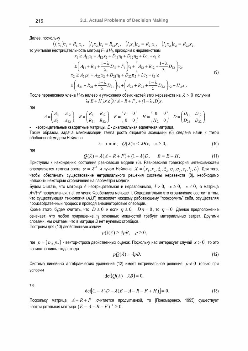
3.1. Actual Problems of Decision Making
216
Далее, поскольку ( ) ( ) ( ) ( ) 222222121211212122111111 ,,, xRcxlxRcxlxRcxlxRcxl ==== ,
то учитывая неотрицательность матриц F1 и H2, приходим к неравенствам
.xHxDRAxDRA
iLcDDxAxAx
,xDRAxFDRA
eLcDDxAxAx
1222222221212121
222221212221212
212121211111111
112121112121111
λλ1
λλ1
ηηλλ1
λλ1
ηη
−⎟⎠⎞
⎜⎝⎛ −
+++⎟⎠⎞
⎜⎝⎛ −
++≥
≥−++++≥
⎟⎠⎞
⎜⎝⎛ −
+++⎟⎠⎞
⎜⎝⎛ +
−++≥
≥+++++≥
(9)
После перенесения члена H2x1 налево и умножения обеих частей этих неравенств на 0>λ получим [ ] ,xD)()FRA(x)HE( λ1λλ −+++≥+
где
⎟⎟⎠
⎞⎜⎜⎝
⎛=⎟⎟
⎠
⎞⎜⎜⎝
⎛=⎟⎟
⎠
⎞⎜⎜⎝
⎛=⎟⎟
⎠
⎞⎜⎜⎝
⎛=⎟⎟
⎠
⎞⎜⎜⎝
⎛=
2221
1211
2
1
2221
1211
2221
1211
000
000
DDDD
D,H
H,F
F,RRRR
R,AAAA
A
- неотрицательные квадратные матрицы, E - диагональная единичная матрица. Таким образом, задача максимизации темпа роста открытой экономики (6) сведена нами к такой обобщенной модели Неймана
,0,)(min, ≥≤→ xBxxQ λλλ (10) где
.,)1()()( HEBDFRAQ +=−+++= λλλ (11) Приступим к нахождению состояния равновесия модели (6). Равновесная траектория интенсивностей определяется темпом роста 1−= λα и лучом Неймана ( )LiexxX ,,,,,,,, 21212121 ηηξξ= . Для того, чтобы обеспечить существование нетривиального решения системы неравенств (8), необходимо наложить некоторые ограничения на параметры модели. Будем считать, что матрица A неотрицательная и неразложимая, ,0,0,0 ≠≥> ccl а матрица A+R+F продуктивная, т.е. ее число Фробениуса меньше 1. Содержательно это ограничение состоит в том, что существующая технология (A,l,F) позволяет каждому работающему “прокормить” себя, осуществляя производственный процесс и проводя внешнеторговые операции. Кроме этого, будем считать, что 0≥D и если 0,0 =≥ ηη D , то 0=η . Данное предположение означает, что любое приращение η основных мощностей требует материальных затрат. Другими словами, мы считаем, что в матрице D нет нулевых столбцов. Построим для (10) двойственную задачу
,0,)( ≥≥ ppBpQ λλ
где ( )21, ppp = - вектор-строка двойственных оценок. Поскольку нас интересует случай 0>x , то это возможно лишь тогда, когда
.)( pBpQ λλ = (12)
Система линейных алгебраических уравнений (12) имеет нетривиальное решение 0≠p только при условии
( ) ,0)(det =− BQ λλ
т.е. [ ] .0)()1(det =+−−−−− HFRAED λλ (13)
Поскольку матрица FRA ++ считается продуктивной, то [Пономаренко, 1995] существует неотрицательная матрица 0)( 1 ≥−−− −FRAE .

KDS 2005 Section 3: Decision Making
217
Пусть также матрица H такая, что FRAH ++≤ (это может выполняться, поскольку 0,0,0 ≥>≥ FRA ). Тогда матрица 0≥−++= HFRAA остается продуктивной, т.е.
существует неотрицательная матрица ( ) 0)( 11 ≥+−−−=− −− HFRAEAE . Именно последнее оказывается наиболее важным требованием. Уравнение (13) можно переписать в виде
[ ] ,0)(det 1 =−+−−− − EDHFRAE µ
где 011
11
>−−
=−
=λλ
λµ при 10 << λ . Наименьшему значению λ соответствует наибольшее
значение µ . Матрица 0)( 1 ≥+−−− −HFRAE . Тогда согласно теореме Перрона-Фробениуса [Пономаренко, 1995] существует число Фробениуса 0>µ и соответствующий вектор Фробениуса 0≥z такой, что
zzDHFRAE µ=+−−− −1)( .
Отметим при этом, что ,)()( 11 DFRAEDHFRAE −− −−−≤+−−−
и поэтому *µµ ≤ , где *µ - число Фробениуса матрицы DFRAE 1)( −−−− . Вернемся теперь к задаче (10), которую перепишем в виде
.0,)(min, 1 ≥≤+−−−→ − xxxHFRAE µµ
Решение этой задачи достигается при zx == ,µµ . При этом темп роста 1µ11
µ11λ 1 >+≥+=−
* , а
также структура выпуска 0≥x . Основной результат данной статьи формулируется в виде такой теоремы.
Теорема 3. Если матрица RA+ продуктивная, матрица FRAH ++≤ , а матрица D не имеет
нулевых столбцов, то в модели (6) существует состояние равновесия с темпом роста µ11λ 1 +=− ,
которому соответствует единственный луч Неймана ( )L,y,,,,,x,x 2212121 ηηξξ , причем: 1) µ - число Фробениуса, x - правый вектор Фробениуса матрицы D)HFRAE( 1−+−−− ;
2) .xlL,xHi,xFl,x,x ===−
== −122111
1
λλ1ηλξ
Литература
[Dorfman, 1958] Dorfman R., Samuelson P.A., Solow R.M. Linear Programming and Economic Analysis, New York: McGraw-Hill, 1958.
[Ашманов, 1984] Ашманов С.А. Введение в математическую экономику. - М.: Наука, 1984.- 296 с. [Пономаренко, 1995] Пономаренко О.І., Перестюк М.О., Бурим В.М. Основи математичної економіки. – К.:
Інформтехніка. 1995.- 320 с. [Иванилов, 1971] Иванилов Ю.П., Петров А.А. Динамическая модель расширения и перестройки производства ( π-
модель). – В кн.: Кибернетику – на службу коммунизму, т.6, М.: Энергия, 1971, с.23-50.
Информация об авторах
Игорь Ляшенко – Киевский национальный университет имени Тараса Шевченко, ул. Васильковская, 42, кв. 44, Киев –22, 03022, Украина; e-mail: [email protected] Елена Ляшенко – Киевский национальный университет имени Тараса Шевченко, ул. Васильковская, 42, кв. 44, Киев –22, 03022, Украина; e-mail: [email protected]

3.1. Actual Problems of Decision Making
218
НЕЧЕТКИЕ МНОЖЕСТВА: АКСИОМА АБСТРАКЦИИ, СТАТИСТИЧЕСКАЯ ИНТЕРПРЕТАЦИЯ, НАБЛЮДЕНИЯ НЕЧЕТКИХ МНОЖЕСТВ
Владимир С. Донченко
Abstract: Рассматриваются вопросы, касающиеся определения нечётких множеств, введения аналога аксиомы свёртки, статистической интерпретации и её связи с аксиомой свёртки, наблюдений нечётких множеств
Keywords:нечёткое подмножество, функция принадлежности, теория множеств
Введение
Нечёткие множества, предложенные Лотфи Заде в работе [1] (см. систематическое изложение в [2]) рассматривались с одной стороны – как метод моделирования, реализующий представления о неопределённости моделируемой ситуации и альтернативный статистическим методам описания неопредлённости, с другой – как теория альтернативная или обощающая класссическую теорию множеств. Претнзии на обобщающий характер теории основывали на нечёткой логике, под которой подразумевалась алгебра оперирования с числами из интервала [0,1] с операциями минимума и максимума в которой справедливы все соотношения булевской алгебры кроме закона исключённого третьего. Однако то, что выходило за рамки булевской алгебры, классическая теорий нечйтких подмножеств не рассматривалось В частности, важнейшим элементом аксиоматики теории множеств является аксиома, которая известная под несколькими названиями: аксиома свертки, принцип абстракции [3] или аксиома выделения [4], которая устанавливает связь между множествами в классическом понимании: “четкими” множествами, - и свойствами элементов универсального множества, собственно, - предикатами, заданными на этом универсальном множестве. В теории нечетких множеств проблема аналога аксиомы свертки (принципа абстракции) исключается из рассмотрения ссылкой на то, что с самого начала рассматриваются нечеткие подмножества, и хотя в обозначении функции принадлежности употребляют элемент, который формально содержит ссылку A на множество: )e(µ A , – тем не менее обозначение A относится к самому нечеткому подмножеству, под которым понимают, собственно, график функции принадлежности[2]:
)Ee )),e(µ,e(A A ∈= , 0≤ Aµ ≤1.
Отсутствие аналога аксиомы свертки или принципа абстракции порождает вопрос о том, какой именно объект или свойство характеризуется нечётко в рамках нечеткого подмножества (E, )e(µ A ). Неявно и только отчасти проблема отсутствия связи между подмножеством и свойством реализуется в понятии лингвистической переменной и её значениях. Именно в рамках понятия лингвистической переменной неявно реализуется принцип абстракции: связь, эквивалентность свойств (предикатов) и подмножеств. Эта неявная реализация принципа абстракции при использовании лингвистических переменных осуществляется рассмотрением для той или иной числовой характеристики: числовой переменной в чётком описании, к примеру расстояния, – свойств, например: “большое”, “среднее” и “малое”, которые связаны с той или иной частью интервала возможных значений расстояния в целом. После этого на соответствующих под интервалах определяется функция принадлежности, которая, собственно реализует нечёткое описание именно отмеченного свойства. Полученные нечеткие подмножества считаются значениями лингвистической переменной. Таким образом, лингвистическая переменная является не просто нечетким подмножеством с соответствующим носителем – а нечеткое подмножество плюс свойство, которое это нечёткое подмножество описывает нечётко, как в упомянутом выше примере со свойствами расстояния. Таким образом в понятии лингвистической переменной неявно реализуется представление об объекте нечеткости: это свойства “большое”, “среднее”, “малое”, а с другой - устанавливается связь между нечеткими подмножествами и соответствующим свойством свойствами.

KDS 2005 Section 3: Decision Making
219
Такой подход только частично реализует связь между свойством и нечетким подмножеством, так как, соответствующие нечеткие объекты являются нечеткими подмножествами заданными на разных носителях E: на подинтервалах исходного множества. Так в примере с расстояниями значениями лингвистической переменной являются нечеткие подмножества, связанные с разными подинтервалами – разными носистелями. В работах [5-6] автора предлагается теоретико-вероятностная интерпретация нечеткого подмножества, точнее: функции принадлежности, – в которой с нечётким подмножеством связывается вполне определённое событие-свойство-предикат. В работе [7] предлагается уточнение определения нечёткого подмножества, в котором подходящий предикат P вводится в само определение нечёткого подмножества: при сохранении общего подхода к заданию нечёткого подмножества носителем и функцией принадлежности, эта последняя приписывается, связывается с предикатом P, который вводится в обозначение функции принадлежности: )e(µ P . Типичным примером такой функции принадлежности, приписываемой определённому событию-свойству является обобщенная логит- и пробит- регрессия. В ней событие-свойство с самого начала присутствует явно: это свойство, которое описывается фиксируется событием 1Y = , которое отвечает совершению покупки и т.д.
Уточнение понятия нечеткого подмножества
Путем решения проблемы построения аналога аксиомы абстракции или выделения для нечетких подмножеств, на взгляд автора, была бы явная ссылка на свойство – или соответствующее ему множество, – неопределенность в определении которой и описывается, собственно, функцией принадлежности. Эта ссылка должен быть явным образом отраженное, например, в обозначении для
функции принадлежности нечеткого подмножества: )e(µ P, где P – соответствующее свойство
(предикат или четкое подмножество). Учитывая наличие аксиомы свертки (абстракции или выделения) для множеств классических, вместо свойства P может стоять подходящее подмножество – классическая – множества E. В рамках такого подхода две функции принадлежности )e(µ P 1 и )e(µ P 2 с P1≠ P2, задают два разных нечетких подмножества, даже, если они совпадают как функции e, e∈E. Определение. Нечетким подмножеством множества E, которое нечетко описывает свойство P на E или соответствующую P множество PE⊆ E, называется пара (E, )e(µ )P( ) или пара (E, )e(µ )P( E ), где: • E - абстрактное множество, которые будем называть универсальным множеством или носителем
нечеткого подмножества; • P – предикат на E, а PE – подмножество множества E, которое отвечает предикату P; • )e(µ )P( – функция двух аргументов: e, e∈E и P из множества предикатов на E. Эту функцию, как и в
классической теории нечетких подмножеств, будем называть функцией принадлежности, прибавляя, что она нечетко реализует или характеризует свойство P или соответствующее множество PE.
Замечание1. По определению, функция принадлежности является функцией двух аргументов: e∈E и P на E или EPE ⊆ . В дальнейшем, учитывая наличие аксиомы свертки в “четкой” теории, если это не обусловлено дополнительно, будем считать функцию принадлежности )e(µ )A( функцией двух аргументов: e∈E и EA ⊆ . Таким образом, нечетким подмножеством с носителем – универсальным множеством – E называется пара (E, )e(µ )A( ). Подытоживая, отметим, что вероятностная интерпретация нечетких подмножеств и пример обобщенных вариантов логит- и пробит- регрессий как функции принадлежности нечеткого множества, а также внутренние потребности теории, связанные с одной стороны с необходимостью явного определения объекта нечеткости, а с другой - с логической полнотой аналогии с “четкими” множествами: введением аналога принципа свертки - приводит к необходимости уточнения понятия нечеткого подмножества. Это уточнение представлено основным определением этого пункта или вариантом, представленным в замечании.

3.1. Actual Problems of Decision Making
220
Вероятностная интерпретация нечетких подмножеств
В общем, основатели теории нечетких подмножеств неоднократно подчеркивали отличие и принципиальную альтернативность теории нечетких подмножеств статистике. Настойчиво подчёркивается, что эта теория является альтернативным средством описания неопределенности, которая отражает степень субъективной уверенности исследователя, хотя сам объект характеризации оставался, как отмечено выше, вне определения нечеткого подмножества. Пример обобщенных вариантов логит- и пробит-регрессий, упоминавшийся выше, не имеет универсального характера хотя бы потому что связан со специальным выбором носителя. С другой стороны, рассмотрение теории нечетких подмножеств как инструмента прикладных исследований: математического моделирования для той или иной предметной области, требовал и требует применения определенной интерпретации нечетких объектов, которая бы выводя за рамки субъективной уверенности, предоставляла возможности говорить о том, какие объективные черты реальных объектов проявляются в виде нечетких объектов и, в частности, отвечала бы на вопрос, что можно считать наблюдением нечеткого множества. Важность последнего вопроса тяжело переоценить, так как на представлении о совокупности объектов и его математическом воплощении в виде абстрактного множества построена вся современная математика.
3.1. Вероятностная интерпретация нечетких подмножеств - дискретный случай
Этот пункт посвящен рассмотрению теоретико - вероятностной интерпретации нечеткого подмножества в классическом варианте определения для случая дискретного носителя. Конечно, эта интерпретация в полной мере касается и уточненного варианта определения. Собственно, теоретико - вероятностная интерпретация является следствием теоремы 1, которая устанавливает связь между функцией принадлежности нечеткого подмножества и системой условных вероятностей по полной группе событий в некотором вероятностном пространстве. Теорема 1. Для любого нечеткого в классическом варианте определения подмножества (E, )e(µ A ) с дискретным носителем E обнаружится такое дискретное вероятностное пространство ( P,B, ΩΩ ), событие Ω∈BA и полная группа событий He: Ω∈BHe , e∈E, – в рамках этого вероятностного пространства, что функция принадлежности )e(µ A представляется системой условных вероятностей в виде:
)e(µ A =PA|He , для произвольного e∈E.
Доказательство. Выберем и зафиксируем любое двоелементное множество с элементами, скажем, α и α . Рассмотрим Ω = Eα,α × . Его элементами являются пары ω вида: ω=( α ,e) или ω=( α ,e) для произвольного e: Ee∈ , – а именно множество Ω , – учитывая дискретность E,– тоже будет дискретной. Пусть pe, pe > 0, e∈E – вероятности любого ряда распределения на E, которые удовлетворяют единому требованию: все эти вероятности ненулевые. С помощью функции принадлежности )e(µ A , e∈E и вероятностей pe, e∈E выбранного ряда распределения определим на булеане Ω вероятность, которая, учитывая дискретность этого множества, задается соответствующим рядом распределения Ω∈ω,pω :
)α(e,ω для ,p))e(µ1(
)α(e,ω для ,p)e(µp
eA
eA
ω⎪⎩
⎪⎨
⎧
=−
== .
Действительно: • для произвольного Ω∈ω 0pω ≥ ;
• ∑∑∑∈∈Ω∈
+=Ee
e),α(Ee
e),α(ω
ω ppp = 1p))e(µ1(p)e(µEe
eAEe
eA =−+∑∑∈∈

KDS 2005 Section 3: Decision Making
221
Определим событие ΩBA∈ и полную группу событий ΩBHe ∈ , e∈E соотношениями соответственно: EαA ×=
He=(α ,e), (α ,e , e∈E. Очевидным образом: A I He=(α ,e). Кроме того: Р He = Р( α ,e)+ Р(α ,e)= pe > 0, P(AI He)=P( α ,e)= )e(µA ·pe,
а, ведь: e
eA
ee
ee p
p)e(µp
)e,α(P)H(P
)HA(P)H|A(P ===I = )e(µA .
Затем: )e(µA = )H|A(P e .
И доказательство закончено. Результат, сформулированный в теореме 1, можно распространить на систему нечетких множеств, которую будем называть полной в понимании следующего определения.
Определение. Систему ))e(µ,E(iA , n,1i = нечетких в классическом определении подмножеств будем
называть полной группой нечетких подмножеств, если для произвольного Ee∈ выполняется соотношение:
∑=
n
1iA )e(µ
i=1.
Теорема 2. Для любой полной нечеткой в классическом варианте определения группы подмножеств ))e(µ,E(
iA , n,1i = одним и тем самым дискретным носителем E обнаружится такое дискретное
вероятностное пространство ( P,B, ΩΩ ), набор событий Ω∈BAi , n,1i = и полная группа событий He: Ω∈BHe , e∈E, – в рамках этого вероятностного пространства, что функции принадлежности
iAµ ,
n,1i = представляется системой условных вероятностей в виде: )e(µiA =PAi|He , для произвольного
e∈E, n,1i = .
Доказательство. Выберем и зафиксируем любое n-элементное множество ℜ с элементами, скажем,
iα , n,1i = : n1 α,,α K=ℜ . Рассмотрим Ω = E×ℜ . Его элементами являются пары ω вида: ω=( α ,e) для произвольных e: Ee∈ , ℜ∈α , а само множество Ω , – учитывая дискретность E тоже будет дискретным. Пусть, как и в доказательстве предыдущей теоремы, pe, pe > 0, e∈E – вероятности любого ряда распределения на E, которые, так же, удовлетворяют единому требованию положительности. С помощью функций принадлежности )e(µ
iA , n,1i = и вероятностей pe, e∈E выбранного ряда распределения на E определим на булеане ΩB множества Ω вероятность, которая, учитывая дискретность этого множества, задается соответствующим рядом распределения Ω∈ω,pω :
)α(e,ω для µ
)α(e,ω для µ
n
1
ω
1
⎪⎪⎩
⎪⎪⎨
⎧
=
==
,p))e(
,p)e(p
eA
eA
n
L
3.1. Actual Problems of Decision Making
222
Действительно: • для произвольного Ω∈ω 0pω ≥ ;
• ∑∑∑= ∈Ω∈
=n
1i Eee),α(
ωω i
pp =∑∑= ∈
n
1i EeeA p)e(µ
i = ∑ ∑
= ∈
n
1i EeeA p)e(µ
i =∑
=
n
1iA )e(µ
i =1.
Определим события Ω∈BAi , n,1i = и полную группу событий Ω∈BHe , e∈E соотношениями соответственно:
EA ii ×α= , n,1i = eHe ×ℜ= , e∈E.
Очевидным образом: Ai I He=( iα ,e), n,1i = , e∈E.
Кроме того: Р He = ∑∈ eHω
ωp =∑=
n
1i)e,α( i
p =∑=
n
1ieA p)e(µ
i = pe > 0, P(AiI He)=P( iα ,e)= )e(µ
iA ·pe,
а, ведь: e
eA
e
i
e
eiei p
p)e(µp
)e,α(P)H(P
)HA(P)H|A(P i===I == )e(µ
iA .
Затем: )e(µiA = )H|A(P ei , n,1i = , Ee∈ .
И доказательство теоремы закончено.
Вероятностная интерпретация нечетких подмножеств - непрерывный случай
Результат предыдущего пункта удается значительно усилить: собственно, к уровню представления системами условных вероятностей дискретного случая, - если носитель E является структурированным, и эта структура является структурой пространства с мерой. Теорема 1. Пусть: • ( E, ( , m )- пространство с мерой; • ))e(µ,E(
iA , n,1i = µ i(e), i > 0 – полная группа нечетких множеств с одним и тем самым носителем E:
• все функции принадлежности )e(µ )A( i , n,1i = являются измеримыми функциями относительно пары σ -алгебр ℑ, £, £– борелевская σ -алгебра в R1.
Тогда: • существует вероятностное пространство (Ω, BΩ, P), • существует дискретная случайная величина ξ со значениями из некоторого дискретного множества
Sp=S1, S2,…,Sn; • существует обобщенная случайная величина (со значениями в E) такая, что для произвольного
n,1i = • )e(µ )A( i = P ξ = Si | η = e , где Pξ = Si | η – условное распределение в.в. ξ относительно в.в. η. Условное распределение является регулярным: для произвольного e:P(B | η= e является вероятностью по B. Доказательство в этом случае воплощает общую идею доказательства дискретного случая построения подходящего вероятностного пространства по условным распределениям.
Наблюдение нечетких множеств.
Уточнение понятия нечеткого множества и соответствующая вероятностная интерпретация дают возможность объективизировать понятие нечеткого объекта и дает возможность говорить о наблюдении нечеткого множества, когда речь идет о применении нечеткости в математическом моделировании.

KDS 2005 Section 3: Decision Making
223
Под наблюдением нечёткого множества можно в уточнённом варианте определения понимать пару (e, P(e))– значения елемента e носителя и значения предиката на рассматриваемом элементе. При таком понимании наблюдения, собственно, речь идёт о предъявляемом элементе и фиксации выполнения или невыполнения свойства Р для этого элемента. Именно такое понимание наблюдения и наблюдаемости имеет место в обобщениях логит- и пробит-регрессии. При построении-оценивании функций принадлежности, например по методу максимального правдоподобия, как это делается в упомянутой выше регрессии или иным способом. При привлечении экспертов для оценивания функции принадлежности, указанные эксперты могут при предъявлении элемента e либо отвечать на вопрос о величине )e(µ )A( i либо – на вопрос о том, отвечает ли e требованию А и давать ответь в виде 0, когда по его мнению отвечает и 0 – когда нет. Способ оценивания функции принадлежности в подходящей параметризации может быть подходящая линейная комбинация функционала метода максимальной правдоподобности и метода наименьших квадратов.
Литература 1. Zadeh, Lotfi. Fuzzy Sets/ Information and Control, 8(3). June 1965. pp. 338-53. 2. Кофман А. Введение в теорию нечетких множеств.- Г.: Радио и связь. 1982.- 322 с. 3. Столл Роберт Р. Множества.Логика. Аксиоматические теории.- Г.: Просвещение.- 1968.-231 с. 4. Куратовский К., Мостовский А. Теория множеств.-М.:Мир.-1970.-416 с. 5. Донченко В.С. Условные распределения и нечеткие множества.//Вестник Киевского университета, 3, 1998. 6. Донченко В.С. Вероятность и нечеткие множества.//Вестник Киевского университета, 4,1998. 7. Донченко В.С. Статистические модели наблюдений и нечеткие множества.//Вестник Киевского университета,
1, 2004.
Информация об авторе
Владимир С. Донченко – профессор, Киевский национальный университет имени Тараса Шевченко, факультет кибернетики, кафедра Системного анализа теории принятия решений; e-mail: [email protected]
ТЕХНОЛОГИЯ КЛАССИФИКАЦИИ ЭЛЕКТРОННЫХ ДОКУМЕНТОВ С ИСПОЛЬЗОВАНИЕМ ТЕОРИИ ВОЗМУЩЕНИЯ ПСЕВДООБРАТНЫХ МАТРИЦ
Владимир С. Донченко, Виктория Н. Омардибирова
Аннотация: предложена технология классификации электронных документов с использованием теории возмущения псевдообратных матриц.
Ключевые слова: классификация, обучающая выборка, псевдообратная матрица,Web Data Mining.
Введение
Одной из важнейших современных прикладных задач классификации является классификация электронных документов. Приложения могут быть самые разные. Например, классификация электронной почты и отсеивания так называемого спама, то есть писем не представляющих интерес для пользователя; или классификация документов по тематике при получении их из такого неструктурированного хранилища как Интернет. Данные задачи относятся к классу задач добычи полезных данных из Интернет (Web Data Mining). В представленной статье описана технология классификации электронных документов по заданным классам. В качестве математического аппарата используется теория возмущения псевдобратных матриц. [1]

3.1. Actual Problems of Decision Making
224
Постановка задачи
Имеется несколько классов электронных документов из некоторой предметной области. Каждый класс характеризуется набором документов-эталонов. Вся предметная область характеризуется некоторым заданным тезаурусом одинаковым для всех классов документов. Необходимо создать и обучить с помощью сформированной из документов-эталонов обучающей выборки классификатор, который будет относить вновь поступающие документы к одному из известных классов. Стандартным в решении задачи распознавания является с одной стороны формирование значимых признаков(Feature Extraction) [2], с другой – выбор подходящий функции близости к формируемым классам.
Основные обозначения
Пусть имеется K классов электронных документов, которые будем обозначать соответственно, kΩ , K,k 1= для которых фиксирован один и тот же тезаурус, количество терминов которого будем
обозначать L. Признаками, по которым будет производиться классификация, выбираются относительные частоты использования терминов тезауруса. Таким образом, каждый документ можно представляется в виде вектора a: )a,...,a(a L
T1= состоящего из относительных частот встречаемости слов из тезауруса в
данном. Пусть kn , K,k 1= – количество документов обучающей выборки, относящихся к каждому из классов. Введём в рассмотрение матрицы kA , K,k 1= , составленные из «частотных» векторов каждого из классов. Очевидным образом каждая из матриц имеет размерность knL× , K,k 1= .
Обозначим среднее векторов обучающей выборки по каждому из классов через ka , K,k 1= :
∑∈
=kak
k an
aΩ
1 , K,k 1= . (1)
Сдвинем каждый из векторов обучающей выборки того или иного класса на среднее по тому же классу, и матрицы, составленные из полученных векторов как по векторам столбцам. Составим новые матрицы, аналогичные kA , K,k 1= . Будем обозначать полученные матрицы, связанные с каждым из классов через kA~ , K,k 1= .
Алгоритм классификации
Алгоритм классификации предлагается строить на основе вычисления векторов ka , K,k 1= и построения сингулярного разложения [1] для матриц kA~ , K,k 1= , характеризующих соответствующие классы. Как известно, в соответствии с сингулярным разложением матрицы допускают представление:
( ) )k(i
r
i
T)k(i
)k(ik
kyA~ λx
1∑=
= , kkk ArankA~rankr == , K,k 1= , где 221 λλ r≥≥K . (2)
Собственные значения iλ и собственные векторы kn)k(i
L)k(i Rx,Ry ∈∈ , kr,i 1= , K,k 1= в данном
представлении могут быть вычислены, например, методом Якоби или методом сингулярного разложения матрицы SVD [3]. Сингулярные разложения (2) матриц классов можно использовать для построения приближений этих матриц, которые в свою очередь будут использованы для построения мер близости к каждому из классов. Эти приближения строятся в два этапа: на первом отбрасываются «старшие члены» сингулярных разложений: слагаемые, отвечающие меньшим значениям модулей собственных чисел; на втором – полученные матрицы используются для построения мер близости к классам. Оценка ошибки,

KDS 2005 Section 3: Decision Making
225
совершаемой при отбрасывании «старших членов» сингулярного разложения, если оставляется sk членов: kk rs < описывается следующим неравенством[1]:
21
1
221
2
1
22λλλ∆ )(x)(x)( )k(
s
r
si
)k(i
)k(s
)k(i
r
si
)k(is k
k
kk
k
kik +
+=+
+=∑∑ ≤≤= , где
( ) kkis)k(
i
s
i
T)k(i
)k(ik rs,yA~
k
k<+= ∑
=∆λx
1, K,k 1=
( ) )k(i
r
si
T)k(i
)k(iis
k
kk
y λx∆1
∑+=
=
(3)
Параметр ks , kk rs < , K,k 1= выбирается из соображений малости ошибки, совершаемой при построении подходящего приближения kA~ , K,k 1= , и как правило sk выбирается так, чтобы
)k(sk 1λ + соответствовало процентам или нескольким процентам от модуля максимального собственного
числа. Такое построение приближения существенно упрощает вычислительную процедуру построения меры близости к каждому из классов: мер, которые можно построить либо на основе исходных матриц
kA~ , K,k 1= , либо их приближений, построенных в соответствии с процедурой, описанной выше.
Меры близости определяются как квадратичные формы с матрицами Rk, K,k 1= , которые строятся на основе подходящих приближений матриц kA~ , K,k 1= ,– которые будем обозначать соответственно
ks,kA~ , K,k 1= – в соответствии с формулами:
( ) ++ ⋅=kk s,k
Ts,kk A~A~R = ∑
=
−ks
i
)k(i
T)k(i
)k(i )()y(y
1
2λ (4)
Процедура отнесения электронного документа, характеризующегося «частотным» вектором )b,...,b(b L
T1= к одному из классов kΩ , K,k 1= производится на основе вычисления для каждого из
них «расстояния» km , K,k 1= до класса, которое определяется выражением:
( ) ( )⎟⎠⎞
⎜⎝⎛ −⋅⋅−= )k(
kT)k(
k abRabm , K,k 1= (5)
Классифицируемый документ будет относиться к тому классу, для которого значение расстояния km , K,k 1= , определяемое в соответствии с (5) будет принимать минимальное значение.
Результаты экспериментов
Для проверки правильности работы предложенной технологии была выбрана книга в электронном формате «The Handbook of Data Mining» [2] размером 689 страниц и состоящая из 3 частей. Соответственно была сформирована обучающая выборка из трех классов по 5 первых документов-глав в каждом классе. После обучения классификатора на его вход подавались главы книги, которые не использовались в обучении классификатора для того, чтобы он отнес их к одному из 3 классов. Для 8 главы первой части подданной на вход классификатора значения функционала (10) равны:
0.01959 0.15240 0.09561
Так как наименьшее значение функционала равно 0.01959, то классифицируемый документ относится к первому классу.

3.1. Actual Problems of Decision Making
226
Выводы
В статье описана технология классификации электронных документов по заданным классам с использованием теории возмущения псевдообратных матриц, которая показала свою эффективность по крайней мере в рассмотренных модельных примерах. Предложенная технология может использоваться для автоматической классификации поступающей электронной почты или для автоматической добычи интересующей информации из сети Интернет (Web Data Mining). Благодаря использованию приближений для псевдообращенных матриц, удаётся существенно повысить скорость работы алгоритма.
Список литературы
Кириченко Н.Ф., Куц Р., Лепеха Н.П. Распознавание трехмерных объектов по ультразвуковым эхо-сигналам // Проблемы управления и информатики.− 1999.− 5− С.110−122.
The Handbook of Data Mining / edited by Nong Ye, LAWRENCE ERLBAUM ASSOCIATES, London, 2003, 689p. Форсайт Дж., Малькольм М., Моулер К. Машинные методы математических вычислений.-М.:Мир,1980.-280 с. Гантмахер Ф.Р. Теория матриц.-М.:Наука,1967.-287 с.
Информация об авторах
Владимир С. Донченко – профессор, Киевский национальный университет имени Тараса Шевченко, кафедра Системного анализа и теории оптимальных решений, e_mail: [email protected] Виктория Н. Омардибирова – аспирантка, Киевский национальный университет имени Тараса Шевченко, кафедра Системного анализа и теории оптимальных решений, e_mail: [email protected]
ВЕКТОРНЫЕ РАВНОВЕСИЯ ВО МНОГОКРИТЕРИАЛЬНЫХ ИГРАХ
Сергей Мащенко
Abstract: There are proposed the necessary and sufficiency conditions of the vector Nash’s equilibria in multicriterion games.
Keywords: Nash’s vector equilibria, multicriterion game.
Введение
Концепция равновесия по Нешу, несомненно, является важнейшим теоретико-игровым инструментом, который наиболее часто применяется в экономике, социологии, экологии. Пусть N – множество игроков. Рассмотрим многокритериальную игру )Ni;U,X(G ii ∈= в нормальной форме [1,2], где n,...,,N 21= - множество из n игроков; iX - множество стратегий і–го игрока, элементы которого называют стратегиями и обозначают через ix , Ni∈ ;
iMjj
ii ))x(u()x(U ∈= - вектор критериев, ii m,...,,M 21= - множество индексов критериев i–го игрока, im - их количество (каждый критерий )x(u j
i представляет собой действительнозначную функцию, определенную на множестве ситуаций игры ∏
∈=
NiiXX ). Каждый из игроков стремится получить по возможности большее значение
всех своих критериев. Если каждый игрок может однозначно определить предпочтение на множестве своих критериев, то в соответствии с методами многокритериальной оптимизации [3], многокритериальную игру можно легко

KDS 2005 Section 3: Decision Making
227
превратить в обычную (однокритериальную) игру, где функциями выигрыша игроков будут свертки критериев, например, Ni),x(umin)x(W j
iji
ji ∈= ρ , где Ni,Mj, i
ji ∈∈> 0ρ , - весовые коэффициенты
соответствующие предпочтению і–го игрока на множестве своих критериев, Ni ∈ . Однако, проблема состоит в том, что во многих игровых ситуациях игрок априори не может определить предпочтение на множестве своих критериев, так как оно уже само становится элементом игры, зависит от других игроков и должно формироваться в процессе игры.
Векторные равновесия
Поскольку во многокритериальной игре выигрыши игроков определяются векторными функциями
iMjj
ii ))x(u()x(U ∈= , Ni∈ , то нам следует определить в данном случае понятия предпочтения.
В этой работе мы будем придерживаться строгой и слабой аксиом Парето [3]. Интерпретация этих аксиом в условиях многокритериальной игры состоит в следующем. Говорят, что ситуация х доминирует ситуацию y по вектору критериев Mj
j ))x(u()x(U ∈= , если Mj),y(u)x(u)y(U)x(U jj ∈≥⇔ f ,
и хотя бы одно неравенство строгое, т. е. )y(U)x(U ≠ , и говорят, что х сильно доминирует y, если Mj),y(u)x(u)y(U)x(U jj ∈>⇔ ff .
Для формализации равновесия Неша в условиях многокритериальной игры нам будут необходимы специальные отношения доминирования, которые мы назовем отношением доминирования по Нешу и слабым отношением доминирования по Нешу. Будем говорить, что ситуация х многокритериальной игры
доминирует по Нешу ситуацию х’ ( 'xxNEf ), которая получается из ситуации х изменением, каким-то, но
лишь одним игроком, своей стратегии, если: )x,'x(U)x,x(U:Ni i\Niii\Nii f∈∃ . В случае
слабого доминирования: 'xxNEff )x,'x(U)x,x(U:Ni i\Niii\Nii ff∈∃⇔ .
В соответствии с отношением доминирования (NEf ) на множестве ситуаций Х определим множество
векторных равновесий Неша (обозначим его через )Ni;U,X(NE ii ∈ ). Оно будет состоять из ситуаций х*, которые не доминируются по Нешу ни одной другой ситуацией, т. е.
*xx:Xx)Ni;U,X(NE*xNE
ii f ∈¬∃⇔∈∈ . (1)
Аналогично определяется множество слабых векторных равновесий Неша
⎭⎬⎫
⎩⎨⎧
∈¬∃=∈ *xx:Xx*x)Ni;U,X(SNENE
ii ff .
Рассмотрим подробнее векторные равновесия Неша. Предположим, что для любой критериальной функции Ni,Mj),x(u i
ji ∈∈ , выполняются условия существования максимума на множестве ситуаций
игры (множество ситуаций компактно, а критериальные функции непрерывны; множество ситуаций конечно и т.п.). Тогда, если провести аналогию к задачам многокритериальной оптимизации [3], то определение векторного равновесия можно сформулировать в следующем виде:
Ni,)*x,y(U*)x(U)Ni;U,X(NE*x i\NiiXy
iiiii
∈=⇔∈∈∈
MaxVect . (2)
Действительно, при фиксированном і (номере игрока) и фиксированном наборе стратегий других игроков i\N*x из (1) получим определение Парето-оптимальной альтернативы i*x для многокритериальной
задачи: )*x,y(U i\NiiXy ii∈
MaxVect .
Рассмотрим пример векторного равновесия Неша для следующей двух-критериальной игры двух лиц:

3.1. Actual Problems of Decision Making
228
A21 A22 A23 (3,3) (3,1) (1,1)
A11 (1,1) (2,2) (3,3)
(2,2) (2,2) (2,2) A12
(1,3) (2,2) (3,1) (1,1) (1,3) (3,3)
A13 (3,3) (2,2) (1,1)
В этом примере: A11, A12, A13 – множество стратегий первого игрока, A21, A22, A23 - множество стратегий второго игрока; векторы выигрышей первого игрока представленные в верхнем левом углу каждой ячейки таблицы, а выигрыш второго – в нижнем правом углу. Интересная особенность примера - отсутствие равновесий Неша в этой игре, если каждый игрок будет оценивать свой выигрыш только по одному (любому) критерию. По определению векторного равновесия получим:
NE= =∩∈∈
)y,(U),y(UA,A,AyA,A,Ay
22232221
11131211
12AMaxArgVect22AMaxArgVect21
(A12,A22).
Условия оптимальности
Сформулируем сначала общие (те, что не основываются на специальных свойствах множества стратегий и критериальных функций выигрыша игроков) условия векторного равновесия Неша, которые будут в некотором роде аналогами условий оптимальности в теории многокритериальной оптимизации [3]. Теорема 1. Для того чтобы ситуация х* была векторным равновесием Неша, необходимо и достаточно, чтобы она была решением системы оптимизационных задач:
NiMk,Mj*),x(u)x,x(u)x,x(umax*)x(u iij
ii\Nij
ii\Niki
Xxki
ii
∈∀∈∀∈≥= ∗∗
∈ , . (3)
Доказательство. Докажем необходимость. Пусть )Ni;U,X(NE*x ii ∈∈ . Тогда по определению (1)
получим: *xx:XxNEf ∈¬∃ . Построим множества ,Mj*),x(u)x,x(uXx*)x(V i
jii\Ni
jiii
i ∈≥∈= ∗
Ni∈∀ . Заметим, что Ni,*)x(V i ∈∀∅≠ . Предположим противное, что
*)x(Vx)x,x(umax)x(u*)x(u:Mk,Ni iii\Ni
ki
ki
kii ∈=<∈∃∈∃ ∗ . Тогда имеем *)x(u)x(u j
ij
i ≥ ,
iMj∈∀ ; *)x(u)x(u ki
ki > . Отсюда, по определению доминирования Неша, получим *xx
NEf , что
приводит к противоречию )Ni;U,X(NE*x ii ∈∉ . Докажем достаточность. Пусть ситуация х* удовлетворяет (3). Предположим противное, что
)Ni;U,X(NE*x ii ∈∉ . Тогда существует такой игрок с номером Ni ∈ , для которого обнаружится
такая ситуация X)*x,x(x i\Ni ∈= , которая *xxNEf , т. е. *)x(u)x(u j
ij
i ≥ , iMj∈∀ , а для некоторого
:Mk i∈ *)x(u)x(u ki
ki > . Отсюда
ijii\Ni
jii\Ni
ki
Xxki
ki Mj*),x(u)x,x(u)x,x(umax)x(u*)x(u
ii
∈≥≤< ∗∗
∈ . Получили противоречие.♦
Следует отметить, что, с вычислительной точки зрения, система задач (3) есть довольно сложной и многоразмерной (количество задач равняется суммарному количеству критериев всех игроков -∑
∈NiiM ),
поэтому целесообразно рассмотреть следующее условие векторного равновесия, которое может быть полезным в определенных случаях.

KDS 2005 Section 3: Decision Making
229
Теорема 2. Пусть )( ii Uϕ - действительнозначная, монотонно возрастающая по каждой переменной функция, Ni ∈ . Тогда, для того чтобы ситуация х* была векторным равновесием Неша, необходимо и достаточно, чтобы она была решением системы оптимизационных задач:
NiMjxuxxuxxUxU ijiiNi
jiiNiiiii ∈∀∈≥= ∗∗ , *),(),( ),((max*))(( \\ϕϕ . (4)
Доказательство. Докажем необходимость. Пусть )Ni;U,X(NE*x ii ∈∈ . Тогда по определению (1)
получим: *xx:XxNEf ∈¬∃ . Построим множества ,Mj*),x(u)x,x(uXx*)x(V i
jii\Ni
jiii
i ∈≥∈= ∗
Ni∈∀ . Заметим, что Ni,*)x(V i ∈∀∅≠ . Предположим противное, что
*)x(Vx))x,x(U(max))x(U(*))x(U(:Ni iii\Niiiiiii ∈=<∈∃ ∗ . Тогда, поскольку функция iϕ
монотонно возрастает по каждой переменной, имеем *)x(u)x(u ji
ji ≥ , iMj∈∀ (из условия
*)(xVx ii ∈ ); iMk ∈∃ : *)()( xuxu k
iki > (из монотонности iϕ ). Отсюда, по определению доминирования
Неша, получим *xxNEf . Поэтому получим противоречие );,(* NiUXNEx ii ∈∉ .
Докажем достаточность. Пусть ситуация х* удовлетворяет (4). Предположим противное, что )Ni;U,X(NE*x ii ∈∉ . Тогда существует такой игрок с номером Ni ∈ , для которого обнаружится
такая ситуация X)*x,x(x i\Ni ∈= , которая *xxNEf , то есть *)x(u)x(u j
ij
i ≥ , iMj∈∀ , а для
некоторого критерия :Mk i∈ *)x(u)x(u ki
ki > . Благодаря тому что функция iϕ есть монотонно
возрастающей за каждой переменной, получим: ij
iiNijiiNiiiXxiiii MjxuxxuxxUxUxU
ii
∈≥≤< ∗∗
∈ *),(),( )),((max))((*))(( \\ϕϕϕ .
Что противоречит начальному предположению.♦ Рассмотрим следствия из этой теоремы для определенных классов функций )( ii Uϕ , Ni ∈ . Без ограничения всеобщности будем считать Ni,Mj,u i
ji ∈∀∈∀> 0 .
Следствие 1. Пусть Ni,Mj, iji ∈∀∈∀> 0ρ , тогда =⇔∈∈ ∑
∈Ni
ji
jiii *)x(u)Ni;U,X(NE*x ρ
Ni,Mj*),x(u)x,x(u)*x,x(umax ij
ii\Nij
iNi
i\Nij
iji
Xx ii
∈∀⎭⎬⎫
⎩⎨⎧ ∈≥= ∗
∈∈∑ ρ .
Следствие 2. Пусть Ni,Mj,,s iji ∈∀∈∀>> 0ρ 0 , тогда ⇔∈∈ )Ni;U,X(NE*x ii
.Ni,Mj*),x(u)x,x(u))*x,x(u(max*))x(u( ij
ii\Nij
is
Ni
si\Ni
ji
ji
Xx
s
Ni
sji
ji
ii
∈∀⎪⎭
⎪⎬
⎫
⎪⎩
⎪⎨
⎧∈≥⎥
⎦
⎤⎢⎣
⎡=⎥⎦
⎤⎢⎣
⎡⇔ ∗
∈∈∈∑∑ ρρ
11
Следствие 3. Пусть Ni,Mj,,s iji ∈∀∈∀>> 0ρ 0 , тогда ⇔∈∈ )Ni;U,X(NE*x ii
.Ni,Mj*),x(u)x,x(u))x,x(u(max*))x(u( ij
ii\Nij
iNi
i\Nij
iXxNi
ji
ji
ii
ji ∈∀
⎭⎬⎫
⎩⎨⎧
∈≥=⇔ ∗
∈
∗
∈∈∏∏
ρρ
Остановимся теперь на слабых векторных равновесиях Неша. Теорема 3. Пусть (без ограничения общности) функции выигрыша всех игроков в ситуации х* принимают положительные значения, т. е. NiMjxu i
ji ∈∈> ,,0*)( . Ситуация х* будет слабым векторным
равновесием Неша тогда и только тогда, когда существуют векторы параметров
Ni,Mj,;)(Mi
iMj
iji
jiMj
jiiii ∈
⎪⎭
⎪⎬⎫
⎪⎩
⎪⎨⎧
∈>===∈ ∑∈
∈+ 0µ 1µµµµ такие, что ситуация х* будет
равновесием Неша в следующей параметрической игре:

3.1. Actual Problems of Decision Making
230
)Ni);x(umin,X()(G ji
jiMj
ii
∈=∈
µµ . (5)
Для слабого векторного равновесия х* можно принять Niii ∈= ,µµ , где +∈ ii Mµ - вектор параметров с компонентами:
Ni,*)x(u
;Mj,*)x(uˆiMk k
iii
jii
ji ∈=∈= ∑
∈ 11λ λµ , (6)
и тогда Ni,ˆ*)x,x(uˆminmax ii\Nij
ijiMjXx iii
∈=∈∈
λµ , т.е. iλ будет выигрышем і – го игрока в равновесии х*
параметрической игры (5). Доказательство. Докажем достаточность. Пусть х* - равновесие Неша параметрической игры (5) при некоторых значениях параметров +∈ ii Mµ , Ni ∈ . Отсюда следует, что для любой ситуации Xx∈ и любого игрока Ni ∈ имеют место неравенства: µµ i
ji
jii\Ni
ji
jiMj
Mj*),x(uˆ*)x,x(uˆmini
∈∀≤∈
, поэтому
существует такой номер критерия iMj ∈ , что Ni,Xx),x(u*)x(u ji
ji ∈∀∈∀≥ . Следовательно
*: xxXxNEff∈¬∃ . Отсюда *x будет слабым векторным равновесием Неша.
Докажем необходимость. Для этого возьмем вектор Ni,ˆ i ∈ µ с компонентами, которые определены формулами (6). Отметим, что +∈ ii Mµ , Ni∈ . Из того, что *x - слабое векторное равновесие следует,
что *xx:XxNEff ∈¬∃ , т.е. )*x,(xu*)(xu:Mj,Ni i\Ni
ji
jii ≥∈∃∈∃ , а значит, неравенство
)*x,(xuˆ*)(xuˆ i\Nij
iji
ji
ji µ µ ≥ . Поскольку const
*)x(u*)(xuˆ
iMk ki
ij
iji === ∑
∈
11λµ , то для любой
ситуации Xx∈ и любого игрока Ni∈ имеют место неравенства: µµ i
ji
jii\Ni
ji
jiMj
Mj*),x(uˆ*)x,x(uˆmini
∈∀≤∈
. Поэтому х* - равновесие Неша параметрической игры (5).♦
Часто бывают полезными специальные условия оптимальности. Рассмотрим следующее.
Теорема 4. (достаточное условие векторного равновесия Неша). Пусть 1RX i ⊆ , iMj
jii ))x(u()x(U ∈= -
на NX векторные функции, Ni∈∀ . Тогда каждое решение х следующей системы алгебраических неравенств:
0; 0 ,Ni,Mk,jx
)x,x(ux
)x,x(ux
,x
)x,x(ux
)x,x(ui
i
i\Niki
i
i\Nij
i
ii
i\Niki
i
i\Nij
i ∈∈<⎟⎟⎠
⎞⎜⎜⎝
⎛
∂∂
∂∂
∂∂
≤∂
∂•
∂∂ (7)
если оно есть внутренней точкой множества ситуаций Х, будет векторным равновесием игры G. Доказательство. Покажем сначала, что для того, чтобы вектор *x был векторным равновесием достаточно существования для каждого игрока Ni∈ такого вектора параметров:
iMjjii )( ∈= ρρ , i
ji
m
j
ji Mj,,
i∈>=∑
=0ρ1ρ
1, что Ni,)*x,y(umax*)x(u
iiii Mji\Ni
ji
jiXy
ji
Mj∈= ∑∑
∈∈∈ ρ . (8)
Действительно, пусть х* удовлетворяет (8). Предположим от противного, что )x,x(u)x,y(u:Mk;Mj),x,x(u)x,y(uXy,Ni i\Ni
kii\Ni
kiiii\Ni
jii\Ni
jiii >∈∃∈∀≥∈∃∈∃ : ,
тогда суммируя эти неравенства с коэффициентами iji Mj, ∈> 0ρ , получим
∑∑∈∈
>ii Mj
i\Nij
iji
Mji\Ni
ji
ji )*x,*x(u)*x,y(u ρρ , что противоречит условию (8).
Запишем достаточные условия экстремума для системы параметрических задач оптимизации (8):

KDS 2005 Section 3: Decision Making
231
,x
)x,x(u
iMj i
i\Nij
iji 0ρ =
∂∂
∑∈
,iMj
ji 1ρ =∑
∈ (9)
,Mj, iji ∈≥ 0ρ 0ρ 2
2<
∂
∂∑∈ iMj i
i\Nij
iji x
)x,x(u (10)
и докажем, что они эквивалентны (7). Без ограничения общности будем считать ранг функциональной матрицы
iMk
i
i\Niki
x)x,x(u
∈⎟⎟⎟
⎠
⎞
⎜⎜⎜
⎝
⎛
∂∂
1максимальным и равным 2 (в противном случае или все критерии игры - константы,
или они совпадают с точностью до констант), тогда одно из решений системы двух уравнений (9), с im
неизвестными для некоторых iMk,j ∈ при условии i
i\Nij
i
i
i\Niki
x)x,x(u
x)x,x(u
∂∂
≠∂
∂ имеет вид:
isi
ji
i
i\Nij
i
i
i\Niki
i
i\Nikij
i Ms;k,js;;;x
)x,x(ux
)x,x(ux
)x,x(u∈≠=−=⎟
⎟⎠
⎞⎜⎜⎝
⎛
∂∂
−∂
∂∂
∂= 0ρ ρ1ρ ρ k
i . (11)
После подстановки (11) в условия (10) получим следующее. Если i
i\Nij
i
i
i\Niki
x)x,x(u
x)x,x(u
∂∂
>∂
∂ , то
00 ≤∂
∂≥
∂∂
i
i\Nij
i
i
i\Niki
x)x,x(u
,x
)x,x(u и имеем неравенства (7), если i
i\Nij
i
i
i\Niki
x)x,x(u
x)x,x(u
∂∂
<∂
∂ , то
,x
)x,x(u
i
i\Niki 0≤∂
∂ 0≥∂
∂
i
i\Nij
i
x)x,x(u , и снова получим (7).♦
Заключение
В заключение следует отметить, что приведенные выше общие условия векторного равновесия (теоремы 1, 2) существенно проигрывают в плане конструктивности условию слабого векторного равновесия (теорема 3), поскольку для их проверки надо решать достаточно сложные системы оптимизационных (не игровых) задач (3) или (4). В случае же слабого векторного равновесия, проверка условий сводится к игровой задаче (5), что позволяет более гибко использовать теорему 3 для решения прикладных задач. С другой стороны, сильная аксиома Парето, на которой базируется понятие векторного равновесия, имеет более широкий спектр применения на практике, чем слабая аксиома Парето, что сужает круг задач, в которых, может быть использована концепция слабого векторного равновесия.
Ссылки
[1] Мащенко С.О., Бабенко О.В. Использование функции полезности для поиска осторожных и доминирующих стратегий в многокритериальной игре// Вестник Киевского университета. Серия: физ.-мат. науки. 2000. 4. с.234-242.
[2] Мащенко С.О. Равновесия Неша в многокритериальных играх// Вестник Киевского университета. Серия: физ.-мат. науки. 2001. 3. с.214-222.
[3] Подиновский В.В., Ногин В.Д. Парето-оптимальные решения многокритериальных задач. М.: Наука, 1982.
Информация об авторе
Мащенко Сергей Олегович – Киевский национальный университет имени Тараса Шевченко, Доцент; Проспект академика Глушкова, 6, Киев – 207, Украина; e-mail: [email protected]

3.1. Actual Problems of Decision Making
232
ЭВОЛЮЦИОННАЯ КЛАСТЕРИЗАЦИЯ СЛОЖНЫХ ОБЪЕКТОВ И ПРОЦЕССОВ
Виталий Снитюк
Аннотация: В статье предложен метод кластеризации сложных объектов и процессов, базирую-щийся на использовании генетического алгоритма. Рассмотрены аспекты его реализации и формиро-вания фитнесс-функции. Представлено решение задачи кластеризации областей Украины по соци-ально-экономическим показателям и осуществлен его сравнительный анализ с результатами класси-ческих методов.
Ключевые слова: Кластеризация, генетический алгоритм.
Введение Процесс поступательного движения к созданию информационного общества сопровождают проблемы, связанные с хранением и обработкой больших массивов данных. Их решение связано с интеллектуаль-ным анализом данных, технологии которого формируются на пересечении искусственного интеллекта, статистики, теории баз данных. К ним принадлежат KDD (knowledge discovery in databases) – обнаружение знаний в базах данных, data mining (“раскопка данных”), OLAP (On-line analysis processing) – извлечение информации из многомерных баз данных и другие. Элементы указанных технологий становятся неотъем-лемой частью электронных хранилищ данных (Warehouses). Значительную часть информации представ-ляют данные, являющиеся социально-экономическими показателями функционирования сложных систем. Большим массивам информации свойственно присутствие шумовых эффектов, их обработка приводит к накоплению совокупной ошибки. Для преодоления указанной проблемы необходимо определять значимые факторы и осуществлять их анализ. Уменьшение информационной энтропии может быть также достигнуто путем группировки объектов и извлечения знаний в меньших и функционально связанных со-вокупностях. Такие процедуры направлены на последовательное преодоление неопределенности. Пер-вым его шагом является решение задачи кластеризации.
Анализ моделей и методов кластеризации Задача кластеризации заключается в определении групп объектов (процессов), которые являются наиболее близкими один к другому по некоторому критерию. При этом никаких предположений об их структуре, как правило, не делается [Мандель, 1988], [Gorban, 2002]. Большинство методов кластеризации базируется на анализе матрицы коэффициентов сходства, в качестве которых выступают расстояние, сопряженность, корреляция и др. Если критерием или метрикой выступает расстояние, то кластером на-зывают группу точек ,Ω такую, что средний квадрат внутригруппового расстояния до центра группы
меньше среднего расстояния до общего центра в исходном наборе объектов, т.е. ,d 22σ<Ω где
.XN
X,)XX(N
dii X
iX
i ∑∑∈∈
=−=ΩΩ
Ω2
Ω2Ω
11 В общем случае, критериями являются:
1. Расстояние Эвклида 21
1
21 ))XX(m
()X,X(dm
jljkjlk ∑
=−= .
2. Максимальное расстояние по признакам ljkjmj
lk XXmax)X,X(d −=≤≤1
.
3. Расстояние Махалонобиса 21
1 ])XX(R)XX[()X,X(d Tlklklk −⋅⋅−= − .
4. Расстояние Хэмминга ∑=
−=m
jljkjlk XX
m)X,X(d
1
1 .

KDS 2005 Section 3: Decision Making
233
Решение задачи минимизации расстояния между объектами равносильно решению задачи минимизации расстояния до объекта, имеющего усредненные характеристики, поскольку, например, для расстояния Хэмминга
.XXXXXXXXXXXXXXXXm
jkj
m
jlj
m
jkj
m
lkj
lj
m
lkj
kj
m
lkj
ljkj
m
lkj
ljkj ∑∑∑∑∑∑∑===
<=
<=
<=
<=
−=−+−≤−+−≤++−=−1111111
2
Задаче кластеризации сопутствуют две проблемы: определение оптимального количества кластеров и получение их центров. Исходными данными для задачи кластеризации являются значения параметров объектов исследования. Очевидно, что определение оптимального количества кластеров является преро-гативой исследователя. Предположим, что число кластеров K задано и mk << , где m - количество объектов. Получим задачу
minXXK
i
im
jij →−∑∑
= =1 1, (1)
где K,i,X i 1= - среднее значение в кластере, ij XX − - расстояние между объектами. Решением задачи
(1) являются центры кластеров ,X i которые могут содержаться среди рассматриваемых объектов, что является достаточно строгим условием, и могут быть представлены любыми точками области исследования. К традиционным методам кластерного анализа относят древовидную кластеризацию, двухвходовое объединение, метод К средних, метод дендритов, метод корреляционных плеяд и метод шаров [Плюта, 1989]. Преимуществами указанных методов является их простота, инвариантность их техники относи-тельно характера исходных данных и используемых метрик. К недостаткам относят слабую формализо-ванность, что затрудняет применение вычислительной техники, а также низкую точность, следствием чего является предварительные оценки структуры пространства факторов и их информативности. Еще одним методом решения задачи кластеризации является использование самоорганизованной карты Кохонена [Kohonen, 1988]. Проблемой использования такой нейронной сети является выбор начальных весовых коэффициентов, непрерывный характер функционирования и эффективность, оценка которой на сего-дняшний день остается проблемой. В качестве альтернативного метода предлагаем использовать генетический алгоритм.
Генетические алгоритмы – неклассический метод решения задачи оптимизации
Первые варианты генетического алгоритма и рассмотрение аспектов его применения появились в работах [Fraser, 1962], [Fraser, 1968], [Bremermann, 1965], [Holland, 1969], [Holland, 1975]. Дальнейшие ис-следования показали его эффективность в решении инженерных, экономических экологических и других проблем. Главной идеей, лежащей в основе построения генетического алгоритма, является использова-ние идей природного отбора, селекции и мутаций. Его канонический вариант содержит такие этапы:
1. Определение генеральной совокупности особей Θ , являющихся потенциальными решениями за-дачи оптимизации фитнесс-функции.
2. Выполнение предварительных шагов алгоритма, заключающихся в определении количества элементов K выборочной популяции ,Ξ причем Θ<<k ; выборе способа нормирования исходных данных; выборе варианта кроссовера, мутации и инверсии, а также соответствующих веро-ятностей.
3. Для каждого элемента k,i,i 1=Ξ∈θ вычисляем значения фитнесс-функции ).(Ff ii θ= 4. С вероятностями ,Pk
i пропорциональными значением if , выбрать две особи и осуществить кроссо-вер, вследствие выполнения которого получим две новых особи.
5. С вероятностью 21 выбираем одну из полученных особей и с вероятностью mP осуществляем
мутацию.

3.1. Actual Problems of Decision Making
234
6. Полученную особь помещаем в новую популяцию nΞ .
7. Повторяем шаги 3-6 ⎥⎦⎤
⎢⎣⎡
2k раз.
8. Переписываем элементы nΞ в популяцию ,Ξ удаляя старые особи. Критерием окончания генетического алгоритма могут выступать следующие условия: сходимость элементов популяции Ξ к одному элементу; максимальное абсолютное отклонение между элементами популяции Ξ будет меньше некоторого положительного числа δ ; максимальное абсолютное отклонения между значениями фитнесс-функции будет меньше некоторого малого положительного числа .ε
Формирование фитнесс-функции задачи кластеризации
Исходными данными задачи кластеризации являются значения факторов (табл. 1). Таблица 1: Значения факторов исследования
1 X11 X12 … X1n 2 X21 X22 … X2n … … … … … m Xm1 Xm2 … Xmn
Предварительно, выполним их нормирование, например, по формуле .xx
xxx
minjmaxj
minjij'ij −
−= Вследствие
такого преобразования значения всех факторов будут лежать в единичном гиперкубе n],[ 10 . Фитнесс-функция реализуется следующим алгоритмом:
Шаг 1. Значение фитнесс-функции положить равным нулю ( .F 0= ) Шаг 2. Задать количество кластеров K и указать значение .m Шаг 3. Выполнить инициализацию матрицы принадлежности элементов к кластерам kT . Шаг 4. Для всех объектов выполнить следующие шаги. Пусть 1=n Шаг 5. Вычислить расстояние от n -го объекта до центров всех K кластеров, которые является осо-
бями из выборочной популяции. Шаг 6. Среди всех расстояний K,j,d j 1= выбрать минимальное qd и отнести n -й объект к q -му
кластеру. Внести соответствующую запись в матрицу kT . Шаг 7. .dFF q+= .nn 1+= Шаг 8. Если шаги 5-7 выполнены для всех объектов, то получено значение фитнесс-функции F , в
противном случае перейти на шаг 5. Очевидно, что алгоритм получения фитнесс-функции можно оптимизировать. Возможность улучшения является его внутренним свойством. Многообразие вариантов операций генетического алгоритма представляют множество внешних свойств процесса получения фитнесс-функции. Возможность решения задачи ее оптимизации также предполагает двоичное и десятичное представление исходных данных. И если в первом случае в процедурах генетического алгоритма доминирующим является равномерное рас-пределение, то во втором – при поиске оптимального решения предпочтение отдается значениям, имею-щим нормальное распределение с математическим ожиданием, совпадающим с центром кластера. Опре-деление оптимальной дисперсии – еще одна задача, которая остается нерешенной.
Кластеризация областей Украины по социально-экономическим признакам
Для проверки эффективности предложенного метода кластеризации были выбраны области Украины. Кластеризация должна была быть осуществлена, исходя из значений социально-экономических показателей. Такими показателями являются:
1X - валовая прибавочная стоимость в расчете на одного человека (в фактических ценах, грн.);

KDS 2005 Section 3: Decision Making
235
2X - территория (тис. кв. км); 3X - инвестиции в основной капитал на одного человека (в сравнительных ценах, грн.); 4X - прямые иностранные инвестиции на одного человека (долл. США); 5X - занятость населения на 10 тыс. человек; 6X - денежные доходы населения на одного человека (грн.); 7X - кредиты, предоставленные субъектам хозяйствования на одного человека; 8X - количество полученных патентов на изобретения на 10 тыс. человек.
В качестве классических методов были выбраны древовидная классификация и метод K средних. Априорно задано два кластера. По методу K средних получены следующие результаты (табл. 2). К первому кластеру отнесены Днепропетровская, Донецкая, Запорожская, Николаевская, Одесская, Полтавская и Харьковская области. Согласно древовидной кластеризации (рис. 1) к первому кластеру отнесены те же области, кроме Донецкой области, хотя она и близка к элементам первого кластера.
Таблица 2
область
1 2 3 4 5 6 7 8 9 10 11 12 13 14 15 16 17 18 19 20 21 22 23 24
кластер
2 2 2 1 1 2 2 1 2 2 2 2 2 1 1 1 2 2 2 1 2 2 2 2
Кластеризация была проведена также с использованием эволюционного моделирования. Критерием окончания вычислительного процесса была выбрана максимальное количество итераций равное 1000. Для тех же двух кластеров и восьми факторов количество переменных (хромосома), для которых проводилась оптимизация фитнесс-функции, составило 16. В выборочную популяцию вошло двадцать элементов. Учитывая, что фитнесс-функция являлась полиэкстремальной, вероятность мутации составила 0, 4. Такое значение увеличило время вычислений, но значительно увеличило точность расчетов за счет выбивания функции из локальных минимумов.
Рис.1 – Результаты древовидной кластеризации Рис.2 – Значение фитнесс-функции

3.1. Actual Problems of Decision Making
236
Рис.3 – Расстояние между центрами кластеров Рис.4 – Координаты центров кластеров
Для контроля за процессом вычислений в режиме реального времени выводилась информация о значении фитнесс-функции на каждой итерации (рис.2); о среднем расстоянии между центрами кластеров (рис. 3); значения центров кластеров (рис. 4). Значение фитнесс-функции уменьшилось с 9106 ⋅ до 11351587, причем на начальных этапах уменьшение происходило гиперболически, а на последних – линейно. Среднее расстояние между центрами кластеров уменьшалось линейно, с постоянно уменьшающейся дисперсией. В результате вычислений получено два центра кластеров. Координаты первого
.,X,X,X,X,X,X,,X,X 34179125544623999150104553 87654321 ======== Координаты второго ,X,X,X,X,,X,X 15554288585300202952 654321 ======
.,X,X 590297 87 == К первому кластеру относятся Днепропетровская, Донецкая, Николаевская, Одесская, Полтавская и Харьковская области. Результаты трех рассмотренных методов являются близкими, что свидетельствует о точности эволюционного моделирования. Его преимуществом является также указание центров кластеров и формализация вычислительного процесса. Как было указано выше, предложенная технология может быть усовершенствована.
Заключение
Предложенный метод эволюционного моделирования, базирующийся на использовании генетического алгоритма, эффективно функционирует при обработке массивов большой размерности, поскольку в нем оптимально сочетаются целенаправленный поиск и элементы случайности, направленные на выбивание целевой функции из локальных минимумов. Никаких предварительных условий для его использования не требуется. Главным условием оптимизации вычислений является правильная алгоритмизация расчета значений целевой функции. Многовекторность процесса улучшения быстроты алгоритма (для генетических алгоритмов особенно актуально) и его точности (поиска глобального минимума фитнесс-функции), а также его востребованность свидетельствуют о необходимости решении задачи оптимизации предложенного метода.
Библиография
[Мандель, 1988] И.Д. Мандель. Кластерный анализ. Москва, Финансы и статистика, 1988. [Gorban, 2002] A.N. Gorban, A.Yu. Zinovyev. Method of Elastic Maps and its Applications in Data Visualization and Data Modelling // Int. Journal of Computing Anticipatory Systems, CHAOS. - 2002. - Vol. 12. - P. 353-369.

KDS 2005 Section 3: Decision Making
237
[Плюта, 1989] В. Плюта. Сравнительный многомерный анализ в эконометрическом моделировании. – Москва: Фи-нансы и статистика, 1989.
[Kohonen, 1988] T. Kohonen. Self-organization and associative memory. – New-York, 2d. ed., Springer Verlag, 1988. [Fraser, 1962] A.S. Fraser. Simulation of genetic systems. J. of Theor. Biol., vol. 2, pp. 329-346, 1962. [Fraser, 1968] A.S. Fraser. The evolution of purposive behavior. In Purposive Systems, H. von Foerster, J.D. White, L.J. Peterson, and J.K. Russel, Eds. Washington, DC: Spartan Books, pp. 15-23, 1968. [Bremermann, 1965] H.J. Bremermann, M. Rogson, S. Salaff. Search by Evolution. In Biophysics and Cybernetic Systems. M. Maxfield, A. Callahan, and L. J. Fogel, Eds. Washington DC: Spartan Books, pp. 157-167, 1965. [Holland, 1969] J.H. Holland. Adaptive plans optimal for payoff-only environments. Proc. of the 2nd Hawaii Int. Conf. on
System Sciences, pp. 917-920, 1969. [Holland, 1975] J.H. Holland. Adaptation in Natural and Artificial Systems. Ann Arbor: Univ. of Michigan Press, 1975. [Skurikhin, 1993] A.N. Skurikhin, A.J. Surkan. Identification of parallelism in neural networks by simulation with language J.
Proc. of the Intern. Cohf. on KPL, APL Quote Quad, Vol.24, No.I, pp.230-237, Toronto, Canada, August 1993.
Информация об авторе
Виталий Снитюк – Киевский национальный университет имени Тараса Шевченко, докторант факультета кибернетики; пр. Акад. Глушкова 2, стр. 6, Киев, Украина; e-mail: [email protected]
СИСТЕМА КАЧЕСТВЕННОГО ПРОГНОЗИРОВАНИЯ НА ОСНОВЕ НЕЧЕТКИХ ДАННЫХ И ПСИХОГРАФИИ ЭКСПЕРТОВ
А.Ф. Волошин, В.М. Головня, М.В. Панченко
Резюме. Дается описание системы технологического прогнозирования, основанной на методе дерева решений. Ставится задача сбора и обработки экспертной информации, предлагаются методы ее обработки, которые позволяют учитывать нечеткость информации и разрешают проблему большой размерности, которая возникает при значительном объеме дерева решений. Приводится описание системы диагностики эпилептических заболеваний.
Ключевые слова. Метод дерева решений, нечеткие экспертные данные, поиск оптимальных путей.
Вступление
Для прогнозирования поведения немонотонных процессов существует целый ряд так называемых методов качественного анализа, которые используют данные экспертов. Одним из наиболее распространенных из них является метод дерева решений, суть которого состоит в представлении развития исследуемого явления в виде некоторой иерархической структуры, которая строится на основе экспертной информации [Тэрано, 1993]. Представляемая система позволяет организовывать опрос экспертов[Макаров, 1982], на основе собранной информации строить дерево решений и на основе его анализа делать прогноз развития явления на определенный период. Для этого ставится задача сбора экспертной информации, ее анализа, предлагаются оригинальные методы, которые ее решают. На основе предложеной системы были созданы такие прикладные СППР:
- система диагностики эпилептических заболеваний; - система диагностики кардиологических заболеваний.

3.1. Actual Problems of Decision Making
238
В процесе их создания проведены опросы экспертов, построены соответствующие деревья решений. Для нахождения прогноза к построенным деревьям применяются указанные методы, основная цель работы которых – найти оптимальные пути в дереве решений и суммарные веса вершин. Представленные результаты являются развитием работ [Волошин, 1999],[Волошин, 2001],[Voloshin, 2003].
Поиск оптимальных путей
Постановка задачи анализа дерерва решений:
пусть KiaayxyxTayxxf iyy
iyyl
l
j
iyyi lljj
,1);,...,),(),(()(),,(1211
021
01
1
1
02
01 =−−∗=
−+∑−
=
, - K оценочных
функционалов для альтернативы (пути) nlyyy l ≤= ),,...,( 1 , l - количество дуг, которые входят в путь y , n - количество вершин в дереве решений, 0
1x - начальная вершина, 02x - конечная вершина.
Тут 0),...,(121
=− ll yyyy aaT , если 0...
13221=
− ll yyyyyy aaa и 1),...,(121
=− ll yyyy aaT иначе, Y - множество
всех возможных путей (то есть множество всех возможных комбинаций N вершин дерева решений). Тогда задача обработки решений имеет вид: 1) в случае задания отношения предпочтения четко: необходимо найти такую альтернативу
),...,( **1
*pyyy = , что )()(:);,...,(; **
1 yfyfyyyyyYy l ≥≠=∈¬∃ , где l -количество элементов в векторе y , при условии
),...,),(),(()(),,(1211
021
01
1
1
02
01 lljj yyyyl
l
jyy aayxyxTayxxf
−+−−∗= ∑
−
=
;
2) в случае задания отношения предпочтения нечетко: необходимо найти такое множество YY ⊆' , что для '' Yy ∈∀ выполняется условие: ', YyYy ∉∈¬∃ , что )()(,,1, ' yfyfKii ii ≤=∀ ;
)()(,,1, ' yfyfKii ii ≥=∀ (если необходимо найти самые длинные пути); или необходимо найти такое множество YY ⊆' , что для '' Yy ∈∀ выполняется условие:
', YyYy ∉∈¬∃ , ),...,( 1 lyyy = , где l -количество элементов в векторе y , что
)()(,,1, ' yfyfKii ii ≥=∀ (если необходимо найти самые коротки пути).
Ни один из существующих на данный моент методов не позволяет решить такую задачу. Поэтому, на основе известных методов Дейкстры и Флойда [Майника, 1981], созданы оригинальные методы поиска на дерерве.
Алгоритм поиска самого длинного пути. Необходимо найти самый длинный путь из вершины s в вершину t . Каждой вершине x соответствует оценка )(xd . Каждая вершина может быть окрашена и раскрашена (лишена окраски). Шаг 1. Окрашиваем вершину s. Пусть syxdsd =−∞== ,)(,0)( . Шаг 2. Для всех вершин пересчитываем:
),()(),(max)( xyaydxdxd += , где ),( xya соответствует длине дуги, которая соединяет вершины y и x . Если же такая дуга отсутствует, то −∞=),( xya . Если −∞=)(xd для всех неокрашенных вершин x и вершина t не окрашена, закончить процедуру алгоритма: в исходном графе отсутствуют пути из s в неокрашенные вершины. Иначе окрасить ту из неокрашеннных вершин x , для которой величина )(xd наибольшая. Кроме того, окрасить дугу, которая ведет в выбранную на даном шаге x . Положим xy = . Если )(xd для неокрашенной вершины x увеличивается, то раскрашиваем ее и соответствующую дугу.

KDS 2005 Section 3: Decision Making
239
Шаг 3. Если для всех неокрашенных вершин −∞=)(xd и вершина t окрашена, то самый длинный путь найден, закончить работу алгоритма. Для этого метода сформулировано и доказано утверждение:
Утверждение 1. Алгоритм нахождения самого длинного пути требует выполнения 35,1 n операций сравнения, где n – количество вершин в дереве.
Для случая задания переходов в дереве решений нечетко, то есть когда ),...,( 1 mijijij aaa = , nji ,1, = ,
m - колличество элементов вектора ija , разработано оригинальный метод нахождения самого длинного пути.
Модифицированный алгоритм поиска самого длинного пути. Необходимо найти самый длинный путь из вершини s в вершину t . Дуги графа заданы нечетко, с помощью векторов. Каждой вершине x соответствует вектор оценок )(xdi . Каждую вершину можно окрасит и раскрасить. Шаг 1. )0,...,0()( =sd i и ),...,()( −∞−∞=xdi для всех sx ≠ , 0=i . Шаг 2. Для каждой неокрашеной вершины x следующим образом пересчитываем величину )(xdi :
),()(),(max)( xyaydxdxd iii += . где вектор ),( xya соответствует длине дуги, которая соединяет вершини y и x , и max рассматривается поэлементно. Если же такая дуга отсутствует, то ),...,(),( −∞−∞=xya . Очевидно, что возможен случай, когда векторы )(xdi и ),()( xyaydi + невозможно сравнить. Тогда
)()( xdxd ii = , та ),()()(1 xyaydxd ii +=+ , 2+= ii . Это значит, что в зту вершину существуют два возможные пути. Если же векторы можно сравнить, то
),()(),(max)( xyaydxdxd iii += та 1+= ii . Таким образом имеем для вершин ix такие характеристики:
))(),...,(()( 1 ikii xdxdxd = .
)( ii xd - это вектор, который определяет длину одного из возможных путей к вершине ix .
После этого выделяем из множества оценок )( ixd паретовское множество [Макаров, 1982]. Если для i -ї окрашенной вершини после выделения паретовского множества размер вектора )( ixd изменился, то раскрашиваем ее. Затем выбираем доминирующие вершины Aixi ∈, , A - некоторые множества, для которых выполняется pxdxdkAjx ipjkj ∀≥¬∃∉¬∃ )()(:; , и окрашиваем их.
Шаг 3. Если все вершины, для которых −∞>)(xd окрашены, и после шага 2 ни одно )(xd не увеличилось, завершить процедуру. Иначе перейти к шагу 2. Для этого метода сформулировано и доказано такое утверждение: Утверждение 2. Модифицированный алгоритм нахождения самого длинного пути требует выполнения
)2ln( 4 KnO операций, где n – колличество вершин в дереве, а K - колличество элементов в векторах, которыми задаются переходы в дереве. При применении метода поиска самого длинного пути и модифицированного метода поиска самого длинного пути для обработки деревьев значительного объема, возникает проблема большой размерности [Волошин, 1989], связанная со значительными временными затратами. Для ее решения создано оригинальный метод локальной оптимизации, на основе известного метода вектора спада [Сергиенко, 1985].

3.1. Actual Problems of Decision Making
240
Модифицированный метод вектора спада. Необходимо найти самый длинный путь из вершины sa в вершину ta . Известен некоторый начальный путь ),...,( ts aaa = , который соединяет эти две вершины. Задаем некоторую окрестность r (глубину поиска). Шаг 1. sy = . Шаг 2. С помощью описанных методов находим самый длинный путь из ya в rya + . Заменяем соответствующий сегмент в пути a ; 1+= yy . Шаг 3. Если try <+ , то перейти к шагу 2. Если же try ≥+ , то находим самый длинный путь из y в t . Заменяем соответствующий сегмент в пути a . Заканчиваем работу алгоритма. Таким образом, улучшая начальный путь a , мы находим оптимальный (локально оптимальный) путь. Для этого метода сформулировано и доказано такое утверждение.
Утверждение 3. Применение модифицировнного алгоритма вектора спада требует выполнения )(3 rKr −∗ операций сравнения, где r – глубина поиска, K – длина начального пути.
Описание инструментальной системы
Дерево решений задается матрицей инцидентностей. В каждой ячейке матрицы находится вектор ija - который задает вероятность перехода из вершины i в вершину j . Он состоит из десяти натуральных чисел 10),,...,( 101 ≤≤ iaaa . Сумма элементов каждой строки равна единичному вектору. Матрица заполняется путем опроса экспертов. Существуют функции: добавление строк и столбцов, дублирование числа, словарь, сохранение таблицы в файле, загрузка таблицы из файла.
Рис. 1
Построение дерева решений (главной таблицы)
Вспомогательная таблица
Инструменты управления главной таблицей
Применение сверток
Блок опроса экспертов
Обработка полученной информации
Вычисление суммарного веса каждой вершины в дереве
Методы поиска оптимальных путей в дереве
Приближенные методы поиска оптимальних путей в дереве
Формирование группы экспертов, тестирование экспертов
END Анализ полученной информации

KDS 2005 Section 3: Decision Making
241
Рис. 2
Эпилепсия
Возраст манифестации
Картина припадков
ЕЕГ ЕЕГ во время припадка
Неврология Психика Нейрорадиология
Етиология
Первые дни жизни
5-10 лет
10-20 лет
Более 20 лет
Во сне Не во сне
Частые
Редкие Вокализации
При сознании Без сознания
Дизартрия
Конбюгирован-ные движения
глаз Дневные
Ночные
Галюцинации
Внешний фактор
Жевательные движения
Жестикулья-торные
автоматизмы
Аура
Покалывания
Нарушения речи
Макро и микросоматогнозии
Дизориентация
Абсансы
Депресия Тонические приступы
Изменение температуры Фокальные
Спайк
Острая волна
Спайк-волна
Острая-волна -
медленная волна
Вспышка
Розряд
Паттерн
Реакция на открытие закрытие
глаз
Реакция на дихание
Без изм.
Голов. боль
Вегет. растройства
Опухоль
Гемипарез
Цереб. парезы
Енцефало-патия
Атаксия
Без изм.
Емоц. растр.
Задержка псих.
развития
Трудности обучения
Поверх-ностность
Экстра-вертность
Тяжелая деменция
Без
Возм. струк-турные изм.
90% струк. наруш
Наследст-венность
Вирус-новос-палит.
Врожд. повреж-дения ЦНС
Травма
Опухоль
Нару-шения коры
1 2 3 4 5 6 7 8 9 10 11 12 13 14 15 16 17 18 19 20 21 22 23 24 25 26 27 28 29 30 31 32 33 34
Сопоставлние симптомов формам эпилепсии
Первые месяцы жизни
1-5 лет

3.1. Actual Problems of Decision Making
242
Для экспертного опроса необходимо воспользоваться формой, которая позволит задать до 10 матриц одинаковой размерности. Каждая такая матрица – это результат сравнения экспертом вариантов вершин, которые могут быть включены в дерево (матрицы jA ). Далее проводится анализ этих матриц в результате которого определяются вершины, которые включаются в дерево, и вероятности, с которыми возможен переход в них из вершины верхнего уровня. Эти результаты заносятся в текущую строку матрицы таблицы, которая описывает уровень дерева решений. После задания матрицы инцидентностей, возможен ее анализ. Для этого необходимо задать две вершины в дереве решений, и будет найден самый короткий (наименее вероятностный) и самый длинный (наиболее вероятностный) путь, соединяющий эти вершины. Так же возможен подсчет общего веса каждой вершины в дереве. Схема работи созданной программной системы поддержки принятия решений изображена на рисунке 1. Созданная инструментальная система применялась для создание СППР, которые успешно решали практические задачи, в частности, для создания системы диагностики эпелептических заболеваний на базе знаний эксперта (одного из авторов). Для этого было построено соответсвующее дерево решений, которое изображено на рисунке 2. На верхних уровнях этого дерева находятся основные характеристики, анализируя которые врач ставит диагноз пациенту. На нижних уровнях собраны конкретные значения, которые могут принимать эти характеристики. В листах этого дерева находятся варианты заболевания, соответствующие международной классификации заболеваний. Расставляя оценки наличия у пациента конкретных симптомов и применяя описанные методы и алгоритмы, врач-эпилептолог может вычислить вес (вероятность) каждого листа (заболевания) или найти самый длинный (самый вероятносный) путь, который соединяет пару заданных вершин, что соответсвует нахождению наиболее вероятностного сценария развития заболевания. Фрагмент дерева решений приведен на рисунке 2. Также, с помощью описанной системы была создана СППР, которая позволяет диагностировать кардиологические заболевания на основе електрокардиограммы. С помощью экспертов было построено аналогичное предыдущему дерево решений, на верхнем уровне которого находятся элементы электорокардиограммы (QRS комплекс, P и S пики и т.д.), на нижних уровнях – конкретные значения этих параметров, а в листах – варианты заболевания (по международной классификации их 65). Как и в предыдущем случаи, анализ построенного дерева решений состоит в вычислении суммарных весов листов и нахождении оптимальных путей в дереве решений.
Вывод
Возможно применение данной системы в таких областях как медицинская диагностика, прогнозирование курса валюты и т.п. Причем точность работы системы зависит только от квалифицированности экспертов.
Библиография
1. [Тэрано, 1993] Т. Тэрано, К. Асаи, М. Сугэно. Прикладные нечеткие системы.- М.: Мир 1993. –345 c. 2. [Волошин, 2001] Волошин А.Ф., Панченко М.В. Прогнозирование нестабильных процессов с помощью метода
дерева решений, на основе метода попарных сравнений для анализа экспертной информации // Труды Международной научно-практической конференции KDS-2001 “Знание – диалог - решение”, Т.1, Санкт-Петербург, 2001. – С.50-53. (англ.)
3. [Волошин, 1989] Волошин А.Ф. Метод локализации области оптимума в задачах математического программирования// Доклады АН СССР, т. 293, 3, 1989. – C. 269-273.
4. [Волошин, 1999] Волошин А.Ф., Панченко М.В., Пихотник Е.П. Экспертная система поддержки прогнозирования курса гривны // Искусственный интеллект, 1999, 2. – C.354-359. (укр.)
5. [Макаров, 1982] Макаров И. М. и др. Теория выбора и принятия решений М.: Наука, 1982. – 328 c. 6. [Волошин, 2001] Волошин А.Ф., Гнатиенко Г.М. Построение коллективной ранжировки на основе меры рангов
объектов // Вестник Киевского Национального Университета, Кибернетика, 4, 2001. – 478 c. (укр.)

KDS 2005 Section 3: Decision Making
243
7. [Сергиенко, 1985] Сергиенко И.В. Математические модели и методы решения задач дискретной оптимизации. – Киев: Наука Думка, 1985.-384 с.
8. [Майника, 1981] Э. Майника. Алгоритмы оптимизации на сетях и графах. - М.: Мир, 1981. – 321 с. 9. [Voloshin, 2003] Voloshin O.F., Panchenko M.V. The System of Quality Prediction on the Basis of a Fuzzy Data and
Psychography of the Experts // International Journal “Information & Application”.-2003.-3. - P. 261-265.
Информация об авторах
Волошин О.Ф., профессор, КНУ им. Тараса Шевченко, факультет кибернетики, Украина, Киев. Головня М.В., врач-эпилептолог, 1-я клиническая больница, Украина, Киев. Панченко М.В., инженер первой категории, КНУ им. Тараса Шевченко, факультет кибернетики; e-mail: – [email protected]
ПРОЦЕДУРЫ ЛОКАЛИЗАЦИИ ВЕКТОРА ВЕСОВЫХ КОЭФФИЦИЕНТОВ ЗА ОБУЧАЮЩИМИ ВЫБОРКАМИ В ЗАДАЧЕ ПОТРЕБЛЕНИЯ
Елена В. Дробот
Abstract: Тhe author analyses the task of an individual consumers’ choice on the set of teaching excerpts. It is suggested to analyse the function of consumer’s value as additive reduction. For localization of the vector of weighting coefficients of additive reduction the procedures based on metrics of distance of the object towards the ideal point are suggested.
Keywords: The theory of consuming, the function of value.
Аннотация: Рассматривается задача индивидуального потребительского выбора на множестве обучающих выборок. Предлагается рассматривать функцию полезности потребителя в виде аддитивной свертки. Для локализации вектора весовых коэффициентов аддитивной свертки предлагаются процедуры, базирующиеся на метрике близости объекта к идеальной точке.
Ключевые слова: теория потребления, функция полезности.
Введение
Типичной задачей в теории потребления математической экономики традиционно считается [Пономаренко, 1994] задача построения (восстановления, определения) функции полезности потребителя, которая определяет его предпочтения относительно определенного набора товаров (благ). При этом рассматриваются, как правило, так называемые “обучающие выборки”: векторные наборы благ
)x,...,x,x(x n21= , каждая компонента которых является количеством единиц соответствующих товаров, n – количество товаров. Цены товаров и бюджетные ограничения считаются заданными. Выбор потребителя характеризуется отношением предпочтения R, суть которого состоит в следующем: о каждых двух наборах благ он может указать наличие (степень) предпочтения или же их равноценность. Априори считается, что выбор потребителем осуществляется в соответствии с его собственной функцией полезности )x(U , значение которой на обучающей выборке ),...,,( 21 nxxxx = соответствует индивидуальной оценке пользователя для этого набора. Задача потребительского выбора состоит в выборе такого потребительского набора, который максимизирует его функцию полезности при заданном бюджетном ограничении:

3.1. Actual Problems of Decision Making
244
( )
⎪⎩
⎪⎨
⎧
≥≤→
,0,
max
xIpx
xU
где p – вектор цен, I – доход потребителя. Классические методы, используемые для определения функции полезности, представляющей бинарное отношение предпочтений R ( ( ) ( ) 2121 RxxxUxU ⇔≥ , для Xxx ∈∀ 21 , ), в общем случае являются достаточно “жесткими”. Основанием для их применения, в частности служат достаточные условия ее существования, которые задаются, например, теоремой Дебре [Пономаренко, 1994]: отношение предпочтения должно быть полным, рефлексивным, транзитивным и непрерывным, множество решений – связным. Если условия Дебре не выполняются (субъективное отношение предпочтения может быть, в первую очередь, нетранзитивным), и функция полезности, которая представляет отношение R не существует, применение классических методов теории потребления затруднено. Предлагается альтернативный подход для определения функции полезности. Считается, что эксперт (потребитель) при оценивании объекта имеет в виду его векторную оценку. Предлагается процедура формализации проблемы, путем замены «векторной оценки полезности» аддитивной сверткой и тогда задача сводится к уточнению весовых коэффициентов аддитивной свертки.
Постановка задачи
Пусть на множестве товаров nRX +⊆ рассматривается конечный набор потребительских товаров (обучающая выборка). Цены товаров считаются заданными, задано также бюджетное ограничение на суммарную стоимость единиц товаров в выборке. Пусть X – множество обучающих выборок хj, Jj∈ , где J - множество индексов выборок, сформированное в рамках бюджетного ограничения. Каждая выборка
Xx j ∈ , Jj∈ , характеризуется своим распределением единиц для каждого товара )x,...,x,...,x(x n
ji
j1
jj = . Множество индексов товаров выборки обозначим Ι, n,...,1I = . Каждой выборке, Xx j ∈ , Jj∈ , ставится в соответствие ее векторная оценка в пространстве товаров Ωn.
В дальнейшем будем рассматривать не само множество значений единиц товаров Ax j ∈ , Jj∈ , а соответствующее ему множество )x( i
jω , Ii∈ , Jj∈ , где ω некоторое монотонное преобразование, которое определяет степень отклонений количественных характеристик от оптимальных значений для каждого товара i
jx , Ii∈ , Jj∈ , и преобразует все значения количественных характеристик товаров к нормализованному виду в интервале [0,1]. Пусть потребитель (эксперт) последовательно задает свои предпочтения на множестве X в виде бинарного отношения предпочтения R. Предлагается следующий подход к решению задачи: предполагается, что при оценке объекта ( в нашем случае – обучающей выборки) эксперт (сознательно или неосознанно) имеет в виду его векторную оценку. Если рассматривать «векторную» функцию полезности в виде аддитивной свертки, то задача сводится к нахождению весовых коэффициентов свертки (1)-(2):
)x()x(Rxx 2i
Iii
1i
Iii
21 ωρ≤ωρ⇔ ∑∑∈∈
, Xxx ∈21 , , (1)
),...,( n1 ρρ=ρ , Ii∈ , 0i >ρ , 1Ii
i =ρ∑∈
, (2)
где (2) - нормированный вектор относительной важности параметров объектов для утверждения эксперта об отношении предпочтения между объектами. Таким образом, задача состоит в локализации весовых коэффциентов аддитивной свертки (1)-(2).

KDS 2005 Section 3: Decision Making
245
Процедуры локализации вектора весовых коэффициентов
Предлагаются процедуры локализации компонент вектора весовых коэффициентов путем последовательного уточнения интервалов изменения соответствующих компонент вектора ρ (гиперпараллелепипеда весовых коэффициентов в пространстве предпочтений):
],,[ Вi
Ii
Нi ρρ=Π∈ρ ∏
∈
)Ii,( i ∈ρ=ρ , ,10 Ві
Нi <ρ≤ρ< Ii,0,1 i
Iii ∈>ρ=ρ∑
∈
(3)
Идеологическим основанием процедур является гипотеза про «идеальную точку», которая отображает «идеальную выборку» в пространстве товаров (вектор предпочтений в пространстве предпочтений), целостный «образ» которой существует у эксперта. Предполагается, что при сравнении обучающих выборок эксперт сравнивает именно их степень близости относительно некой метрики к «идеальной» выборке с оптимальным распределением единиц товаров. Для преобразования всех значений единиц товаров хjі, Ii∈ , Jj∈ , к нормализированому виду в интервале [0,1] применяется, в частности, следующая формула [Волкович, 1993]:
i0
iopt
ij
iopt
ij
xxxx)x(
−−
=ω , (4)
где хji∈Х, Ii∈ , Jj∈ ; хopti∈Х, Ii∈ , - наиболее желательное количество единиц і-го товара на множестве возможных выборок: х0i∈Х, Ii∈ , - наименее желательное количество единиц і-го товара на множестве возможных выборок. Будем считать, что хopt и х0 могут быть заданы непосредственно экспертом на множестве допустимых обучающих выборок. С учетом (4), обобщенный критерий, который отображает суммарное отклонение j-го объекта, Jj∈ , от оптимальных значений, запишется как
i0
iopt
ij
iopt
Iiii
j
Iii
optj
xxxx)x()x,x(D
−−
ρ=ωρ= ∑∑∈∈
, Jj∈ .
Последняя формула является метрикой близости вектора хj∈ X , Jj∈ , представляющего распределение единиц товаров в j-й выборке к некоторому идеальному (оптимальному) вектору распределений хopt = (хopt1, хopt2,…хoptn), взвешенных в пространстве товаров. Формула (1) запишется в виде:
)x()x(Rxx 2i
Iii
1i
Iii
21 ωρ≤ωρ⇔ ∑∑∈∈
),(),( 21 optopt xxDxxD ≤⇔ , Xxx ∈21 , .
Последнее неравенство можно интерпретировать таким образом: утверждение “выборка х1 предпочтительней выборки х2 ” обозначает, что в пространстве товаров Ωn точка, которая соответствует выборке х1, находится на меньшем расстоянии по отношению к идеальной точке, чем точка, которая соответствует выборке х2. В случае же отношения равноценности выборок соответствующие им точки в Ωn находятся на одинаковом расстоянии от точки, соответствующей идеальному объекту. Процедуры локализации вектора весовых коэффициентов (2) представляют собой фактически две процедуры: процедуру уточнения интервалов весовых коэффициентов (3) и процедуру отсеивания из первоначального множества рассматриваемых обучающих выборок «неперспективных» выборок. Процедуры базируются соответственно на утверждениях 1 и 2, приводимых ниже. Доказательства этих утверждений, обобщенные для случая задания экспертом предпочтений в метризированнной форме, приводятся в работе [Волошин, 2003].
Утверждение 1. Вектор предпочтений, соответствующий равноценным выборкам в пространстве предпочтений Е1, определяет границы интервалов изменения весовых коэффициентов товаров, что численно выражается:
)x()x()x()x( 2i
Ii
Н)s(i
1i
Ii
В)s(i
2i
Ii
Н)s(i
1i
Ii
В)s(i
ssj
2ss
i1
ssj
2ss
i1
ωρ+ωρ=ωρ+ωρ ∑∑∑∑Π∈ρ
∈Π∈ρ
∈Π∈ρ
∈Π∈ρ
∈
, Xx,x 21 ∈ ,

3.1. Actual Problems of Decision Making
246
где ρі(s)В, ρі(s)Н, i∈І, - соответственно верхняя и нижняя границы і-го интервала весовых коэффициентов на s-й итерации сравнений; ∅≠>= ))()(:( 21
1 xxiI ii ωω , ∅≠≤= ))()(:( 212 xxiI ii ωω ,
21 IIIi ∪=∈ . Таким образом, гиперпараллелепипед весовых коэффициентов (ГВК) на (s+1)-ом шаге станет равным:
[ ]∏∏∈
++
∈
+ ρρ×ρρ=Π21 Ii
В)s(Н)1s(В)1s(i
Ii
Н)s(i
1s ,],[ . (5)
Нахождение вектора предпочтений, соответствующего равноценным объектам в [Волошин, 2003], предлагается осуществлять решением n уравнений вида:
0))x(()x(())x()x(( 2i
Ii
1ii
2i
Ii
1ii
21
=ω−ωρ−ω−ωρ∈∈
, Xx,x 21 ∈ , Ii,0,1 iIi
i ∈>ρ=ρ∑∈
. (6)
Утверждение 2. Условием отсеивания объектов ωj, Jj∈ , из множества Хs является непринадлежность ГВК вектора, который проходит через начало координат и точку ω(хj ), х∈Хs, Jj∈ , то есть ρ(ω(хj))∉П(s+1). Вектор весовых коэффициентов определяется по формуле [Волкович, 1993]:
)a(/)a(:))a((qlIq Il
lj
tj
itIt
iij ∑∏∏
≠∈ ∈
≠∈
ωω=ρρ=ωρ=ρ .
Процедуры локализации вектора весовых коэффициентов используются в следующей человеко-машинной процедуре. Шаг 1. Выделение конечного множества обучающих выборок X на бесконечном множестве
потребительских товаров. Первоначальный ГВК полагается равным единичному гиперкубу. Шаг 2. Выбор экспертом двух выборок х1 и х2 из множества Хs в ГВК Пs, s =1,2,...(шаг сужения ГВК) с
указанием факта предпочтения или эквивалентности. Шаг 3. Построение системы уравнений вида (6). Нахождение решения системы уравнений. Шаг 4. Уточнение границ ГВК по формуле (5). Если гиперкуб П(s+1) удовлетворяет эксперта, то
окончание процедуры. Иначе переход к следующему шагу. Шаг 5. Выделение множества «перспективных» выборок Х(s+1) (Х(s+1)⊆Х(s)) в ГВК П(s+1) и предъявление
их эксперту для выбора очередных двух объектов с указанием для них отношения предпочтения.
Шаг 6. Присоединение выборок, указанных экспертом на предыдущем шаге к множеству рассмотренных и исследование на полученном множестве условия транзитивности. Если транзитивность не нарушается, то увеличение номера итерации: s=s+1 и переход к шагу 2. Если же транзитивность нарушается, то исключение этих выборок из множества рассмотренных объектов и переход на шаг 6.
Итерационный процесс завершается, когда эксперта удовлетворяют найденные интервалы изменения весовых коэффициентов товаров. Для нахождения коллективных решений на базе формализованных таким способом интервальных индивидуальных оценок, можна применить, например, методы, предложенные в [Гнатиенко, 2002].
Выводы
Предложенные процедуры, не требуя полной матрицы парных сравнений обучающих выборок, позволяют на множестве бинарных отношений восстановить функцию полезности потребителя. Кроме того, задание вектора весовых коэффициентов в виде интервалов можно интерпретировать и как отображение нечеткости в социально-экономических системах. Поэтому предложенные процедуры позволяют уменьшить уровень неопределенности в нечетких моделях принятия решений. Автор благодарит проф. Волошина А.Ф. за поставленную задачу.

KDS 2005 Section 3: Decision Making
247
Библиография [Пономаренко, 1994] Пономаренко О.І. Системні методи в економиці, менеджменті та бізнесі. – К.: Наукова думка,
1994. – 242 с. [Волкович, 1993] Волкович В.Л., Волошин А.Ф. и др. Модели и методы оптимизации надежности сложных систем /
Под ред. Михалевича В.С. – К.: Наукова думка, 1993. – 312 с. [Волошин, 2003] Волошин А.Ф., Гнатиенко Г.Н., Дробот Е.В. Метод косвенного определения интервалов весовых
коэффициентов параметров для метризированных отношений между объектами // Проблемы управления и информатики, 2003, 2. – с. 34 - 41.
[Гнатиенко, 2002] Гнатієнко Г.М., Дробот О.В., Санько-Новік М.О. Агрегування матриць парних порівнянь // Праці міжнародної школи-семінару “Теорія прийняття рішень”, Ужгород, УжНУ, 2002. – С. 27.
Информация об авторе
Дробот Елена Витальевна – Кировоградский педагогический университет имени В. Винниченко, кандидат технических наук, доцент. Кировоград, Украина. Е-mail: [email protected]
НЕЧЕТКИЕ МОДЕЛИ МНОГОКРИТЕРИАЛЬНОГО КОЛЛЕКТИВНОГО ВЫБОРА
Алексей Ф. Волошин, Николай Н. Маляр
Аннотация: Для многокритериальной задачи с конечным числом альтернатив определяется нечеткая задача достижения “точки удовлетворения лица, принимающего решения”. Предлагаются различные типы “точек удовлетворения ЛПР”, в качестве функций принадлежности предлагаются различные типы сверток, для выбора которых учитываются психосоматические характеристики экспертов. Задача обобщается на случай принятия коллективного решения.
Ключевые слова: коллективный выбор, многокритериальная оптимизация, нечеткая модель, свертка критериев, точка удовлетворения.
Введение
Одна из наиболее общих постановок задачи принятия коллективного решения, имеющая многочисленные приложения в экономике, политике и других областях человеческой деятельности, сводится к следующей математической модели [1]:
max)( →xUi , pIi ,1=∈ , Xx∈ , (1) где iU – функция полезности i-го лица, принимающего решение (ЛПР), X – множество альтернатив (ситуаций). Будем рассматривать модели, в которых множество альтернатив X конечно, nX = , каждая
альтернатива Xx j ∈ оценивается i-м ЛПР набором критериев iK с “универсального” набора
mJi ,1=∈ , оценка альтернатив осуществляется каждым ЛПР независимо, каждый ЛПР имеет свой “тип” функции полезности (определяемой той или иной сверткой “своих” критериев), каждый ЛПР при формировании решения использует свой “принцип оптимальности”. К такой постановке сводится, например, задача формирования комплексных целевых программ [2], в которой в качестве альтернатив выступают множества проектов, связвнных в составные альтернативы причинно-следственными связями, в качестве целей – политические, социальные, экономические и научно-технические критерии: “Увеличение действенности социальной защиты”, “Повышение уровня экономики”, “Повышение уровня науки и культуры”, “Информатизация стратегических направлений развития государственности, безопасности и обороны”, “Улучшение состояния окружающей среды” и т.д.

3.1. Actual Problems of Decision Making
248
([2], С. 340–349, всего 162 целей). Естественно, что оценки таких разнообразных целей различными экспертами, министерствами и ведомствами будут существенно отличаться, отличаться будут и “принципы оптимальности” – от пессимистического (при оценке, например, “экологических” критериев) до оптимистических (при оценке, например, информатизации). При решении поставленной задачи, отличающейся очень высоким уровнем неопределенности, субъективизмом в выборе критериев, оценках альтернатив по ним, естественным будет использование нечеткого анализа [3] для описания субъективной компоненты модели и учет психологических характеристик как отдельных экспертов, так и их коалиций с целью уменьшения “субъективной неопределенности” (см. доклад А.Ф. Волошина “О проблемах принятия решений в социально-экономических” в настоящем сборнике ).
Постановка задачи нечеткого выбора Рассмотрим вначале случай 1=p (один ЛПР). Задача (1) тогда задается одной матрицей решений
)( ijKK = , mi ,1= , nj ,1= (2) где ijK – оценка по i-му критерию j-й альтернативы.
Не ограничивая общности, предположим, что все альтернативы пренадлежат множеству Парето [4], а наилучшей считается альтернатива, для которой все оценки достигают своего максимального и минимального значения. Пусть все оценки – положительные числа, иначе применяем преобразование:
ijj
ijj
ijij KKKK −⎟⎟
⎠
⎞
⎜⎜
⎝
⎛+=′ minmax (3)
Таким образом, множество альтернатив X представляет собой некоторое подмножество эвклидового m мерного пространства mR ++ , каждая альтернатива рассматривается как точка )( ij
j Kx = , Ii∈ , Jj∈ .
Введем точку “удовлетворения ЛПР” mRT ++∈ и опишем множество точек “близких” к этой точке как нечеткое множество
)(, xxA AT µ= , mRXx ++⊂∈ . (4) где )(xAµ – функция принадлежности нечеткого множества TA , характеризирующая “степень принадлежности” элементов Xx∈ нечеткому множеству TA . “Точка удовлетворения ЛПР” T может как принадлежать множеству X (т.е. быть достижимой), так и не принадлежать X (быть недостижимой, например, “идеальной”). Задача выбора теперь сводится к выбору “наилучшей” (по некоторому критерию оптимальности) альтернативы TAx ∈* . Опишем построение функции принадлежности )(xAµ . Предположим, что известна матрица ЛПР (2) и задана точка его “удовлетворения” ( ) miitT ,1== . Опредилим оптимальную безразмерную оценку достижения “точкой удовлетворения ЛПР” оптимальных значений критериев следующим образом:
⎭⎬⎫
⎩⎨⎧ −−−−= iijjijjiiji
ji tKKtKtx max;minmax1 , Ii∈ , Jj∈ . (5)
Построение функции принадлежности Для построения функции принадлежности, как свертки заданных критериальных оценок, предлагается использование следующих сверток критериев эффективности (при условии их равноважности):
∑=
= m
iji
jA
x
mx
1
2
1)(µ , m j
i
m
i
jA xx
1
3 )(=∏=µ ,
m
xx
m
i
ji
jA
∑== 14 )(µ ,
m
xx
m
i
ji
jA
∑== 1
2
5)(
)(µ (6)

KDS 2005 Section 3: Decision Making
249
Как известно, между этими свертками существует следующая субординация: )(2 xAµ ≤ )(3 xAµ ≤ )(4 xAµ ≤ )(5 xAµ , Xx ∈∀ (7)
Последнее означает, что привыборе, например, с помощью “наиболее пессимистической” свертки 2µ “наилучшей” точки TAx ∈* , степень принадлежности ее множеству точек, “близких к точке удовлетворения ЛПР”, будет всегда меньшей, чем при использовании “оптимистической” свертки 5µ . Значит, предлагаемая модель позволяет учитывать достижение определенной “степени удовлетворения ЛПР” от его субъективных особенностей, учитываемых при выборе критерия оптимальности и точки удовлетворения. Таким образом, “объективизация” субъекта накладывается на субъективное описание объекта (см. доклад А.Ф. Волошина).
Точки удовлетворения ЛПР
В качестве “точек удовлетворения ЛПР” предлагается использовать точки iT , 6,1=i , с координатами:
ijji Kt min1 = , ∑=
= n
j ij
i
K
nt
1
2
1, n
ij
n
ji Kt
1
3
=∏= ,
n
Kt
n
jij
i
∑== 14 ,
n
Kt
n
jij
i
∑== 1
2
5 , ijji Kt max6 = . (8)
Учитывая, что между предлагаемыми точками справедлива аналогичная (7) субординация, можно опредилить “степень удовлетворения ЛПР” при выборе конкретной свертки и различных точек удовлетворения.
Методы нечеткой многокритериальной оптимизации
Теперь определенным образом модифицируются “классические” методы многокритериальной оптимизации. Метод идеальной точки. Пусть y = (y1, …, yn) идеальная точка. Зададим правило выбора: выбирается альтернатива x ∈ X, для которой функция принадлежности нечеткому множеству ”близка к идеальной точке” максимальна. Метод с учетом количества доминирующих критериев. Пусть заданы точка удовлетворения T и матрица решений (2). Для каждой альтернативы строятся оценки по следующему правилу:
⎪⎩
⎪⎨⎧
≥<
=.,1,,
ijj
ijjjij
i KtеслиKtеслиx
y
Дальше для каждого вектора оценок jy строится функция принадлежности нечеткому множеству (4) согласно одной из формул (6). Правило выбора: выбирается альтернатива, для которой количество доминирующих критериальных оценок наибольше и/или функция принадлежности принимает максимальное значение.
Заключение
При переходе к общему случаю (количество ЛПР p>1, критерии для каждого ЛПР неравноценны) предлагается применить методы обработки экспертной информации (при усреднении оценок экспертов), учитывающие психосоматические особенности экспертов [6] (степень “реалистичности”, “риска”, “независимости” и т.д). При организации “групповой” экспертизы (все множество экспертов разбивается на коалиции, оценивающие, например, экологические, экономические, социальные, технические и т.д. параметры), необходимо учитывать принципы группового мышления [7].

3.1. Actual Problems of Decision Making
250
Библиография
1. Дж. Харшаньи, Р. Зельтен. Общая теория выбора равновесия в играх. – С.-Петербург: Экономическая школа, 2001. – 406 с.
2. В.Г. Тоценко. Методы и системы принятия решений. – Киев: Наукова думка, 2002. – 382 с. 3. С.А. Орловський. Прблемы принятия решений при нечеткой исходной информации. – М.: Наука, 1981.– 207 с. 4. И.М. Макаров, Т.М. Виноградская и др. Теория выбора и принятия решений. – М.: Наука, 1982.– 328 с. 5. Э. Мушик, П. Мюллер. Методы принятия технических решений. – М.: Мир, 1990. – 208 с. 6. А.Ф. Волошин, М.В. Панченко (ММС). 7. J.L. Janis, L. Mann. Decision making: a Phychological analises of Conflict, Choice and Commitment. – New York: Free
Press, 1977.
Информация об авторах
Волошин Алексей Федорович – Киевский национальный университет имени Тараса Шевченко, доктор технических наук, проффесор. Киев, Украина. Е-mail: [email protected] Маляр Николай Николаевич – Ужгородский национальный университет, кандидат технических наук, доцент. Ужгород, Украина. Е-mail: [email protected]
АЛГОРИТМ ПОСЛЕДОВАТЕЛЬНОГО АНАЛИЗА И ОТСЕИВАНИЯ ЕЛЕМЕНТОВ В ЗАДАЧЕ ОПРЕДЕЛЕНИЯ МЕДИАНЫ СТРОГИХ РАНЖИРОВАНИЙ ОБЪЕКТОВ
Павел П. Антосяк, Григорий Н. Гнатиенко
Аннотация: Рассматривается задача нахождения результирующего ранжирования объектов по индивидуальным ранжированиям, заданных экспертами. Предлагается алгоритм, основанный на последовательном анализе вариантов и условии ацикличности решения. Приводятся результаты вычислительного эксперимента.
Ключевые слова: последовательный анализ, результирующее ранжирование.
Введение
Задачи ранжирования (упорядочения множества объектов по степени проявления некоторого свойства) относятся к одной из основных задач экспертного оценивания [1]. Суть задачи состоит в определении полного порядка на множестве объектов, которые сравниваются, по заданному частичному порядку. Среди задач принятия решений проблема линейного упорядочения объектов выделяется большим количеством конкретных применений и безусловной актуальностью темы. Эта проблема традиционно находится в центре внимания исследователей и количество работ, посвященных вопросам построения оптимальных в том или ином смысле линейных порядков (или квазипорядков) на множестве объектов, которые сравниваются, очень велико [2]. Практическое применение задач ранжирования очень разнообразно [3]. Такие задачи возникают, например, при решении проблемы определения последовательности загрузки и разгрузки транспортного космического корабля; нахождение последовательности устранения неисправностей некоторой системы; комплексном анализе качества продукции; анализе характеристик продукции и выделении главных показателей качества; нахождении узких мест в некой сложной системе, которая имеет такие свойства как устойчивость (например, живучесть), управляемость, самоорганизация; проектирование каналов связи между узлами в информационно-вычислительных сетях; экспертного оценивания различных проектов развития некоторых отраслей или научных исследований; планирование построения жилья и т.п.

KDS 2005 Section 3: Decision Making
251
Будем рассматривать задачи качественного и количественного ранжирования. Суть задач состоит в том, что необходимо ввести отношение порядка на множестве объектов, которые сравниваются. При этом с целью обеспечения большей объективности полученных результатов упорядочение объектов осуществляется группой экспертов. При решении таких задач на этапе задания экспертной информации наиболее широкое применение нашел метод парных сравнений. Но известно, что во многих задачах бинарные отношения, которые представляют мнение экспертов и коллективное мнение экспертной группы, часто содержат контуры (циклы), поэтому анализу этих задач посвящено множество работ [4]. Одной из самых распространенных задач ранжирования есть задача нахождения результирующего ранжирования по ранжированиям (или матрицам парных сравнений, которые соответствуют бинарным отношениям в общем случае нетранзитивным), заданных экспертами. Для вычисления результирующего отношения (которое принадлежит некоторому классу – в нашем случае классу строгих ранжирований) вводится мера близости (как правило, выбирается метрика Хемминга [5]) и выбирается критерий качества результирующего отношения (наиболее распространенным и обоснованным считается вычисление медианы заданных отношений). При этом получают сложную комбинаторную задачу, для решения которой необходимы специальные алгоритмы.
Постановка задачи
Пусть на фиксированном множестве объектов Aa ∈ν , n,...,1=ν , експертами заданы матрицы парных сравнений iP , kIi ,...,1=∈ , где kn, – соответственно количество объектов и экспертов. Элементы
1,1−∈ipνη матриц iP представляют собой результат сравнения і-м экспертом объектов νa и ηa , n,...,1, ∈ην .
Одним из методов нахождения результирующего ранжирования есть вычисление медианы Кемени-Снелла [6]:
( )∑∈ℜ∈
∈Ii
i
RPRdArgR ,min* ,
где ℜ – множество всех матриц, которые соответствуют строгим ранжированиям n объектов (ранжирования и матрицы, которые им соответствуют, будем обозначать одинаковыми символами), ( )iPRd , – расстояние Хемминга между R и iP .
Для решения проблемы вычисления точного решения сложной комбинаторной задачи, NP – сложной в сильном смысле, предлагается алгоритм, который основан на последовательном анализе вариантов [7]. Задача нахождения результирующего ранжирования объектов в изложенной постановке формализируется в классе однокритериальных комбинаторных моделей:
( ) min→−=∑∑∈ ∈Jj Ii
jij xcxf , (1)
1,10 −=∈ jj Xx , 2/)1(,...,1 −==∈ nnNJj , (2) 0XDx A ⊂∈ , (3)
где ∏∈
=Jj
jXX 00 – множество всех возможных векторов вида νηrx j = , ( ) ( ) 2/11 ννην +−+−= nj ,
n≤≤≤ ην1 , νηr – элемент матрицы парных сравнений; AD – множество векторов, которые
соответствуют ацикличным отношениям; ijc – j-я компонента вектора, построенного по матрице iP , заданной і-м экспертом.
Алгоритм определения строгого результирующего ранжирования
С учетом модификации процедур sW для однокритериальных моделей и процедур анализа и сужения множества допустимых вариантов, базирующихся на условии ацикличности решения, опишем алгоритм анализа и отсеивания недопустимых элементов задачи (1)–(3).

3.1. Actual Problems of Decision Making
252
Шаг 1. Вычисление значения ( ) 2maxmin* ss
s fff += , где ss ff maxmin , – соответственно минимальное и максимальное значение целевой функции на s-й итерации, s=0,1,2,...:
∑= ∈
−=N
jjj
Xx
s xcfsjj1
min min , ∑= ∈
−=N
jjj
Xx
s xcfsjj1
max max .
Шаг 2. Применение процедуры sW , суть которой состоит в отсеве элементов множества sjX ,
NJj ,...,1=∈∀ , которые не могут принимать участие при построении решения sXx∈ . Условие отсева имеет вид:
∑∑∑≠∈ ∈ ∈∈
−−−>−
jtJt Ii
titXx
ijsIi
jij xccfxcstt
minarg*
если отсев недопустим, переход к шагу 7. Иначе – к следующему шагу. Шаг 3. Анализ множества допустимых вариантов, основанный на условии ацикличности решения. Если отсев недопустим, переход к шагу 7. Иначе – к следующему шагу.
Шаг 4. Вычисление границ изменения целевой функции sfmin , sfmax . Если границы изменились, то есть 1
minmin−> ss ff или 1
maxmax−< ss ff , переход к шагу 1, иначе – к шагу 5.
Шаг 5. Допустимый отсев: ∅≠sjX для ∀ Jj∈ . Если на множестве sX существуют полные
допустимые решения и общее количество возможных решений ( )∏ ∈= JjXX sj
s , , велико для прямого перебора, переход к следующему шагу. Иначе – к шагу 8.
Шаг 6. Уменьшение значения *sf – выбор, например, методом дихотомии ( ) 2min
**1
sss fff +=+ . Переход
к шагу 2.
Шаг 7. Наращивание *sf – выбор, например, методом дихотомии из интервала ( )s
ss fff max**
1 ,∈+ . Переход к шагу 2.
Шаг 8. Если количество возможных элементов на множестве sX не велико, то путем прямого перебора находим решение *x . Если такое решение единственное и удовлетворяет неравенству
2/)( maxmin* ss
sJj
jij fffxc +=≤−∑∈
, то оно есть искомым решением и соответствует результирующему
ранжированию.
Вычислительный эксперимент
Описанный алгоритм был реализован в программной среде Delphi, вычислительный эксперимент проводился на ПЭВМ с тактовой частотой процессора 1,53 ГГц. Исследовалась задача (1)-(3) с
20050 ÷=n , данные генерировались случайным образом. Изучалась интенсивность отсеивания в зависимости от размерности задачи и времени работы процессора при сужении допусков по целевой функции до **
1 ss ff −= +ε , ∅=+1sX . При 1210≤sX решение находилось прямым перебором (работа процесса порядка 20–30 мин.). Если за один час работы процесса ( 1310>sX ) решение не было найдено, то на суженом множестве генерировалось решение с
использованием эвристических процедур. Рассматривались δεx решения, где ε – точность по целевой
функции, δ – точность по ограничениям [7]. Авторы выражают благодарность проф. Волошину А.Ф. за помощь при подготовке работы.

KDS 2005 Section 3: Decision Making
253
Библиография 1. Литвак Б.Г. Меры близости и результирующие ранжирования// Кибернетика. 1983. 1. – С. 57-63. 2. Миркин Б.Г. Анализ качественных признаков и структур. М.: Статистика. 1980. – 319 с. 3. Левин М.Ш. Современные подходы к оценке эффективности плановых и проектных решений в
машиностроении. Обзорная информация. Сер.С–9. Автоматизированные системы проектирования и управления. М.: ВНИИТЭМР. 1987. Вып.3. – 56 с.
4. Гнатиенко Г.Н., Микулич А.Ю. Методы метризации качественных ранжировок объектов. Киев. ун-т. – Киев. 1993. Библиогр.: 6 назв. Рус. Деп. вУкрНИИНТИ 10.03.93. 432–Ук93. – 10 с.
5. Макаров И.М., Виноградская Т.М. и др. Теория выбора и принятия решений: Учебное пособие. М.: Наука, 1982.– 328с.
6. Кемени Дж.Г., Снелл Дж.Л. Кибернетическое моделирование. М.: Советское радио. 1972. 192 с. 7. Волошин А.Ф. Метод локализации области оптимума в задачах математического программирования// Докл.АН
СССР, т.293, 3, 1987. – С. 234–237.
Информация об авторах
Антосяк Павел Павлович – Киевский национальный университет имени Тараса Шевченко, аспирант. Киев, Украина. Е-mail: [email protected] Гнатиенко Григорий Николаевич – Киевский национальный университет имени Тараса Шевченко, кандидат технических наук. Киев, Украина.
ОДИН ПОДХОД К МОДЕЛИ ТЕОРИИ ИНВЕСТИЦИОННОГО АНАЛИЗА С УЧЕТОМ ФАКТОРА НЕЧЕТКОСТИ
Ольга В. Дьякова
Аннотация: рассматривается классическая модель Гари Марковица, которая используется для формирования оптимального портфеля ценных бумаг; недостатки вероятностного описания прибыльности ценной бумаги и анализируется в качестве такого описания использование теории нечётких множеств; рассматриваются расчетные формулы степени риска неэффективности инвестиций на основании предположения о том, что показатель эффективности инвестиций – треугольное нечёткое число, где коэффициент рассчитывается на основании критического и фактического значений прибыльности портфеля ценных бумаг.
Ключевые слова: принятие решений, степень риска, эффективность инвестиций, нечёткие числа, прибыльность.
Введение
Начиная со второй половины XX-го столетия, большое внимание уделяется построению теоретической базы теории инвестиций. Она получила настолько значительное распространение среди экономистов, что говорят о её революционном развитии. То внимание, которое уделяется портфельным инвестициям, полностью отвечает радикальным изменениям, которые произошли во второй половине двадцатого столетия в экономике промышленно развитых стран. На месте отдельных изолированных региональных финансовых рынков возник общий международный финансовый рынок. Отметим, что традиционный подход к инвестированию, который имел преимущество до возникновения классической теории, имеет два недостатка. Во-первых, он «атомистический», поскольку в нём основное внимание уделялось анализу поведения отдельных активов. Во-вторых, он «одноизмеримый», поскольку основной характеристикой актива является исключительно прибыльность, тогда как другой фактор – риск – не получает чёткой оценки при инвестиционных решениях. [3]

3.1. Actual Problems of Decision Making
254
Базовой среди классических моделей является модель Гари Марковица. На сегодняшний день эта модель используется на первом этапе формирования портфеля активов при распределении капитала, который инвестируется, по разным типам активов. Вероятностный подход Марковица имеет, однако, некоторые модельные характеристики не полностью соответствующие реальностям фондового рынка. Это слабость гипотезы про статичность случайных процессов. Классическая теория, вероятно, констатирует статичность случайных событий в тех условиях, где имеет место статическая однородность выборки событий. Но однородность в силу неисполнения одинаковости условий наблюдения может нарушаться. Изменилось рыночное окружение фирмы и, соответственно, изменилась рыночная позиция эмитента. Следовательно, риск убытков по данной бумаге падает или растёт; но причина этих колебаний внешняя, она не имеет прямого отношения к эмитенту, то есть, не свойственна ему. Поэтому нельзя говорить про статичность случайного процесса доходности ценных бумаг. Если нет статичности случайных процессов дохода по ценным бумагам, тогда нет и статической связи между этими случайными процессами. Когда коэффициенты корреляции задаются константами, предусматривается, что раз и навсегда известен характер причинно-наследственной связи между доходностями двух типов бумаг. Но характер рассмотренной причинности не может быть описанным экспертом полностью точно, а только с некоторой степенью приближения. Намного больше правды в выводах эксперта, когда он вместо чисел употребляет лингвистически нечёткие высказывания с той или иной степенью уверенности. Неопределённость в этом случае имеет двойной характер: с одной стороны – нечёткость в описании самой ситуации, а с другой стороны – неуверенность эксперта при различии одной ситуации от другой. [2] Существенным преимуществом теории вероятности является многовековой исторический опыт использования вероятностей и логических схем, построенных на их основе. Но, когда неопределённость относительно будущего состояния объекта исследования теряет черты статической неопределённости, то классическая вероятность, как измеримая в процессе опытов характеристика массовых процессов, уходит в неизвестность. Ухудшение информационной обстановки вызывает к жизни субъективную вероятность, однако сразу возникает проблема истинности вероятностных оценок. Субъект, который принимает решение, приписывая вероятностям точечные значения в процессе некоторого виртуального пари, исходит из соображений собственных экономических или других преимуществ, которые могут быть деформированы перекрученными надеждами и эмоциями. В рамках существующей интерпретации возникают две проблемы - непосредственный учёт влияния эксперта на процесс принятия решения и уменьшение влияния индивидуальных характеристик эксперта (учёт его «объективных психосоматических особенностей познания действительности»). [1] Предложенный принцип иллюстрируется ниже на прикладной модели задачи принятия решения Гари Марковица в теории инвестиционного анализа.
Метод анализа эффективности инвестиций, модель Г. Марковица
Рассматривается модель Гари Марковица, которая используется для формирования оптимального портфеля ценных бумаг. Она основывается на минимизации риска портфеля при заданном уровне доходности:
1 1
min,n n
p i j iji j
V x x v= =
= →∑∑ при 1
1;n
ii
x=
=∑ 0, 1,ix i n≥ = ; *
1
n
i ii
x m m=
=∑ . (1)
где xi – представляющий вектор (вектор частиц вложений); Ri – случайная величина (величина, которая по результатам исследования может принимать то или иное значение, заранее неизвестно какое именно), которая определяет норму дохода i-той ценной бумаги; ряд значений Ri1 … RiT является реализацией данной случайной величины на временном отрезке T; mi - ожидаемое значение доходности i-той ценной бумаги ( Mi im R= ); vij – ковариация доходности i-той та j-той ценных бумаг. В качестве описания доходности ценных бумаг используются треугольные нечёткие числа, которые моделируют экспертное высказывание следующего типа: “Доходность ценной бумаги по окончанию периода владения ожидаемо равно r и находится в расчётном диапазоне [r1, r2]”. При этом эксперт отказывается от вероятностного описания доходности, отрезает слабовероятностные случайные результаты по двум сторонам от ожидаемого значения r (вероятность таких результатов при

KDS 2005 Section 3: Decision Making
255
нормальном распределении не равно нулю) и формирует расчётный коридор, в котором ожидается уровень доходности ценной бумаги. При этом за r эксперт принимает или наиболее ожидаемое, или среднее значение доходности с расчётного коридора. Функция принадлежности нечёткого числа имеет треугольный вид, если степень субъективной уверенности эксперта в отношении доходности равно нулю за пределами расчётного коридора значений доходности, а максимум этой уверенности, равный единице, достигается в точке r . Эксперт уверен, что r определённо попадёт в какой-либо расчётный коридор доходности, как бы не изменялись границы этого коридора. Приведённый способ описания ожидаемой прибыльности в форме нечёткого числа автоматически снимает все проблемы, связанные с учётом связи ценных бумаг по тенденциям. Если прибыльность ценной бумаги – треугольное нечёткое число, а прибыльность портфеля – линейная комбинация прибыльности компонент, тогда результирующий вид доходности портфеля также известен. Пусть ( )1 2, ,i i ir r r r= – прибыльность по i-той ценной бумаге, треугольное нечёткое число. Тогда прибыльность портфеля также является треугольным нечётким числом:
min 1 max 21 1 1
, ,n n n
i i i i i ii i i
m m x r m x r m x r= = =
⎛ ⎞= = = =⎜ ⎟⎝ ⎠
∑ ∑ ∑ , (2)
Зафиксируем m* – критическое значение прибыльности портфеля. Если фактическое значение прибыльности m окажется ниже m*, то считается, что портфель был сформирован неэффективно. Степень риска неэффективности инвестиций по предположению, что показатель эффективности инвестиций – треугольное нечёткое число, определяется по формулам:
min
min
max
max
0, * ,1(1 ln(1 )), * ,
11 (1 )(1 ln(1 )), * ,
1, * ,
p
при m m
R при m m mV
R при m m m
при m m
α αα
α αα
<⎧⎪ −⎪ + − ≤ <⎪= ⎨ −⎪ − − + − ≤ <⎪⎪ ≥⎩
(3)
где min
maxmax min
max
* , * ,
1, * ,
m m при m mm mR
при m m
−⎧ <⎪ −= ⎨⎪ ≥⎩
(4)
min
minmin
min
maxmax
max
max
0, * ,* , * ,
1, * ,* , * ,
0, * .
при m mm m при m m mm m
при m mm m при m m mm m
при m m
α
<⎧⎪ −⎪ ≤ <⎪ −⎪⎪= =⎨⎪ −⎪ < <
−⎪⎪ ≥⎪⎩
(5)
Отличием полученной модели от стандартной является то, что в качестве фактора риска выступает не стандартное отклонение портфеля, а степень риска неэффективности инвестиций. Стандартные подходы, ориентированные на разработку алгоритмов, которые обеспечивают сходимость к точному решению в классическом понимании, не столько решают поставленные проблемы, сколько создают иллюзию их решения. Проблема состоит не в нахождении с какой-либо точностью решения задачи при неточных данных, а в нахождении интервалов изменения компонент решения. [Ужгород]
Благодарности
Автор благодарен профессору Волошину А.Ф. за помощь при написании статьи.

3.1. Actual Problems of Decision Making
256
Библиография 1. Волошин А.Ф. Проблемы принятия решений в социально-экономических системах.//Труды школы-семинара
«Теория принятия решений» - Ужгород, 2004 – с.15. 2. Недосекин А.О. Применение теории нечётких множеств к задачам управления финансами//Аудит и финансовый
анализ. – 2000. – 1 - с. 15-21. 3. Орловский С.А. Проблемы принятия решений при нечеткой исходной информации. – Москва: Наука, 1981. 4. Шарп У, Александр Дж, Бейли К. "Инвестиции.", М. 1997. 5. S. A. Ross, R. W. Westerfield, J. Jaffe, Corporate finance. – the McGraw-Hill Companies Inc., 1996. 6. Voloshin O.F., Panchenko M.V. The System of Quality Prediction on the Basis of a Fuzzy Data and Psychografphy of the
Experts// “Information Theories & Applications”, 2003, Vol.10, 3.-P.261-265. 7. William N. Goetzmann. In Introduction to Investment Theory //
http://viking.som.yale.edu/will/finman540/classnotes/notes.html.
Информация об авторе
Дьякова Ольга Владимировна – Киевский национальный университет им. Т. Шевченко, факультет кибернетики, аспирантка, Киев, Украина; e-mail: [email protected].
MODEL OF ACTIVE MONITORING
Sergey Mostovoi, Vasiliy Mostovoi
Abstract: Active monitoring and problem of non-stable of sound signal parameters in the regime of piling up response signal of environment is under consideration. Math model of testing object by set of weak stationary dynamic actions is offered. The response of structures to the set of signals is under processing for getting important information about object condition in high frequency band. Making decision procedure by using researcher’s heuristic and aprioristic knowledge is discussed as well. As an example the result of numerical solution is given.
Keywords: math model, active monitoring, set of weak stationary dynamic actions.
Introduction
The distinctive feature of seismic monitoring is the particular, seismic frequency range, encompassing infrasonic and low range of a sound spectrum. The characteristics of each monitoring object are slowly varied in time, but at the same time sometimes processes might be occurred is too rapid. The seismic monitoring deals with the large size objects, down to the sizes of a terrestrial Globe. Because of mankind anxiety on possible earthquakes, the extremely passive monitoring has a deep history, but at latest time, the active monitoring is often used. The active monitoring is such an experiment, which one is connected to generation of sounding signal of a different type, both on a spectral band, and on duration and power, down to atomic explosions. But in active experiment only monitoring approach enables to obtain ecological pure result, i.e. without any of appreciable influencing on an environment. Monitoring is a set of regime observations, and condition of observations and the characteristics of sounding signal depend on the purposes of given investigation. There are many such purposes, but, from our point of view, we select two basic one. It is dynamics of variations happening in investigated object, and it is detail of estimations, which characterize this object. Despite of large discrepancy of these two purpose, the approaches both to experimentation and to processing receivable data are very close, as well as problems, originating at it. To problems, first of all from the ecological point of view, it is necessary to refer necessity to realize active monitoring of investigated object by low-power signals, commensurable with a level of a natural background. This circumstance results that the estimation of sounding signal parameters, passing the studied object, i.e. signal response of an investigated system on a sounding signal, is hampered because of a low signal-noise proportion.

KDS 2005 Section 3: Decision Making
257
Therefore there is a necessity for the special conditions of experiment and applying special, sometimes very composite, signal processing procedures of an investigated system response. The used above words "the regime observations" consider rigid stability in implementation of a condition. It means stability of monitoring time characteristic and parameter stability of a sounding signal, i.e. invariance of its spectral characteristic. With evidence it is clear, that always there is an extreme accuracy of arguments describing a signal and arguments temporary experiment providing. In this article the problem is put: when and to what arguments the instability is essential, in what it results, and how to eliminate its influencing, if it is possible? First of all, it is necessary to construct a mathematical model of experiment, in which one the most essential moments of monitoring process would be reflected, including both processes, and, accompanying this process background noise, and natural hum noise. The prior knowledge of noise stochastic process will allow largely weakening its influencing on deriving of estimation obtainment of process arguments, which one is perceived as a useful signal. This slackening is reached by optimization of processing procedures, which is taking into account prior statisticians of noise stochastic processes. In a series of treatises [1-4], the separate aspects of a reduced problem were regarded. Into the given paper there is an attempt to summarize earlier reviewed the approach to procedure modelling of active experiment, analysis of experiment parameters instability influence and optimization of procedure processing of observed data, by yardsticks taking into account the characteristics of a natural background noise, instability of sounding signal parameters and consequences caused by this instability.
The Mathematical Model of Active Monitoring
The math model of i-th experiment in a serial from M -th ones is proposed. In active monitoring serial can be introduced as follows:
( ) ( ) ( ) ( ) ( )T,t,tntH*h,,tSty iiiiii +∈+= τττ , (1)
where i is number of experiment, ( )tyi - response of environment to an sound signal ( )ii htS ,,τ , depending
from vector of parameters ih , which one is convoluted with reacting of environment ( )tH on a delta-function signal ( )tδ , ( )tni an additive noise accompanying experiment, T - duration of one experiment, ( )Tii +ττ , - time period of i -th experiment conducting of, and ∗ - a convolution operator symbol. The experiment is constructed in such a manner that energy of a signal, registered by sensors, [ ( ) ( ) ]tHhtSE i *,
r and energy of
a natural background ( )[ ]tnE i are commensurable in the selected metric, it means, that influencing of experiment on a state of the environment is negligible. In the pattern that circumstance is taken into account, that the non-linear phenomena in experiment can be neglected, a linear routine of the specification statement of interplay of environment and exploring signal by the way convolutions therefore is selected. Let's mark, that the convolution is described by following integral:
( ) ( ) ( ) ( ) ,dtSHtH*tS τττ0
−= ∫∞
(2)
The full experiment is defined by following model
∑=
=M
ii )t(y)t(y
1 (3)
As a time of experiment T we shall consider the time for which one the reaction level of environment to an exploring signal becomes less then some level ε , which one can be selected depending on a level of a natural background. For example, in the metric TC
ii T >>ΓΓ++ ;),( ττ is instituted from a condition:
ε≤))t(ymax( i ; ),T(t ii Γττ ++∈ for iτ∀ (4) Certainly ε , and after it and T as well, is exclusively selected by the feeling of explorer heuristics, his point of view to experiment and a priori estimations of a noise ( )tn power. As it was noted, the monitoring guesses a serial from M experiments, i.e. .,1 Mi =

3.1. Actual Problems of Decision Making
258
The Model of an Exploring Signal
Let's consider, that the signal ( )ihtS , depends on the vector of parameters iNii hhh ,...,1= , which components are define the shape and energy of signal. It is naturally to consider that a signal is physically realizable, i.e. to be fitting two conditions: causality and stability. The same conditions are natural to the reacting of the environment ( )tH as well.
( ) ( )⎪⎭
⎪⎬⎫
⎪⎩
⎪⎨⎧
<
≥=
00
0
t,
t,h,tSh,tS i
i
rr
; ( )( )∫∞
∞<0
2dth,tS i
r (5)
Causality means, that if the signal has been started at the moment iτ , it means that the experiment has begun at this moment and up to this moment the signal did not exist.
( ) ( )⎪⎭
⎪⎬⎫
⎪⎩
⎪⎨⎧
<−
≥−−=
0τ0
0τττ
i
iiiii
t,
t,h,tS,h,tS
rr
(6)
In a condition of causality we at once consider also a condition of stationary that is reflected in the dependence of a signal on a difference of time t and the signal start moment iτ The stability means, that for any value ε of an energy level in the metric 2L there is such value of T , that
( )( )∫∞
<T
i dthtS ε2
,r
. for ih∀ (7)
The last circumstance allows determining duration of one experiment T , for this purpose it is necessary, that the level ε was less or much less then the energy level of a natural background. It is possible to consider iτ as one of the component (for example, with a zero subscript) of a vector of arguments, which are defining the signal and which are non-linear - including in the pattern of a signal. The duration value of T is a value of deterministic argument, for example, which is equal to the last component of vector h
r. Let’s try to represent other non-linear arguments of a signal. The signal can be introduced as a linear
combination of known functions (for example, fragment of a vector of orthogonal functions ( ) T,,t)k,t( iiiiik +−⋅− τψτχωτ 0 , N,k 1= at an interval of length T .
( ) ( )T,,t)k,t(h,h,tS iiiN
kiikikii +−⋅−= ∑
=τψτχωττ
10
r (8)
Here is i0ω - a sample unit of random argument 0ω , which defines system of functions ),,,( ψωτϕ tr
, and ψ is the applicable phase for this system
( ) N,...,k,T,,t)k,t(),,,t( k 1τψτχωτψωτ =+−⋅⋅−=r
(9) Here is characteristic interval function ( )T,,t +− τψτχ , which is also a non-linear characteristic of the signal model, as well as argument T ,
( ) ( )( ) ⎭
⎬⎫
⎩⎨⎧
+−∉+−∈
=+−;T,t,,T,t,
T,,tiii
iiiiii τψτ0
τψτ1τψτχ .
Let's consider argument 0ω as one more component of arguments vector hr
, namely 1+Nh . Then ψ - 2+Nh ,
and T we shall consider as a 3+Nh component of vector 3,...,0, +== Nkhh k
r.
In this case a sound signal in experiment with number i will be ( )ihtSr
, .
So, the signal model is a random function which is supposed to be physically realizable and a stationary, which one is completely instituted by a random vector h
r, N parameters of which one are linearly entered into
the model.

KDS 2005 Section 3: Decision Making
259
Under consideration is a case, when set of vectors ,,1 ..., Mhhrr
is sampling from set of probable values of vector
hr
with a priori known distribution )(hPr
. It means, that the stochastic nature of process ∑=
=M
ii tyty
1
)()( is
defined by a random vector hr
and stochastic additive noise )(tn . As a determined component into this process is a response of environment ( )tH on a testing signal such as a delta-function. This response contains the environment information. As fluctuations of arguments of an exploring signal is determined and linearly, through the convolution equations, are connected to a signal ),( ihts
r, registered by sensors on an exit of an observation
system, that, allowing identifications (2) for a convolution ∗ , we shall obtain
)t(H)h,t(S)h,t(s ii ∗=rr
and ( ) ( ) ( ) ( ) 30τττ +==+∈+= Niiiiiii hT,h,T,t,tnh,tsty . (10)
Hereinafter we shall esteem only response of environment ( )ihtsr
, . Let's decipher separated values of a vector of
components, defining both signal ),( ihtSr
and response of environment ( )ihtsr
, . First, try to separate arguments, which are included linearly and non-linear into the model.
( )30201
10 χ ++=
+ +−⋅⎟⎠
⎞⎜⎝
⎛ ⋅−= ∑ iNiN,iiN
kN,iikiki hh,hh,t)kh,ht(h)h,t(S
r (11)
0iτ is the component of vector ihr
with zero index, 0iω - 1+N , and T - 2+N -th of a component.
Function vector ( ) N,...,k,T,,t)k,t()h,t( k 1τψτχωτ =+−⋅⋅−=
rr (12)
might be set of convenient for approximation an exploring cue of functions or piece orthonormalized on a spacing ( )T,0 of basis functions. The approximating of an exploring signal in seismic survey by the way of damped sine wave can be regarded as the example
( ) ( )T,,ttsintexp)h,t(S iiiiiiii +−⋅−⋅⋅−⋅= τψτχτωαθr
. (13) In this case vector of free parameters of the pattern, which defines the signal, is
,T,,,,,hh iiiiiiki ψωαθτ==r
50,...,k = and has only five components, from which only the second one
1ih is entered into the model linearly. In general, and relevant for practice of seismic sounding case, the signal is represented by the way of approximating piece of its expansion in a series of orthonormalized base, as in the expression (6). The response of environment in i th experiment will be
( )T,,td)(H)k,t(h)h,t(s iiiN
k
T
iikikii
i
+−⋅⎟⎟
⎠
⎞
⎜⎜
⎝
⎛
⎟⎟⎠
⎞⎜⎜⎝
⎛⋅⋅−−= ∑ ∫
=
+τψτχττωττ
1
τ
τ
r (14)
Taking into account above-mentioned result of a serial from M trials )(ty becomes:
( ) ( ) ( ) ( )
( ) ( ) ( )TM,t,tnT,,t
d)(H)k,t(htntH*h,tSty)t(y
iiii
M
i
N
k
T
iikikM
iii
M
ii
i
i
⋅∈++−⋅
⎟⎟
⎠
⎞
⎜⎜
⎝
⎛
⎟⎟⎠
⎞⎜⎜⎝
⎛⋅⋅−−=+== ∑ ∑ ∫∑∑
= =
+
==
0τψτχ
ττωττ1 1
τ
τ11
(15)
Let's define:
( ) ∫+
⋅⋅−−+−=⋅−T
iikiiiiiiki
i
d)(H)k,t(T,,t),k,t(~ τ
τττωτττψτχψωτ . (16)
With allowance for (16) model of monitoring becomes:
( ) ( )TM,t,tn),k,t(~h)t(y iiiikN
kik
M
i⋅∈+⎟
⎠
⎞⎜⎝
⎛ ⋅−= ∑∑==
0ψωτ11
(17)

3.1. Actual Problems of Decision Making
260
Model of Additive Noise )(tn
In this place we shall note, that for the further analysis the aprioristic knowledge of statistical characteristics of noise ( )tn~ is important. The ideal situation is a knowledge of aprioristic distributions of all sections of stochastic process ( )tn~ , but in our case would be enough to know only its first moment ( )[ ] )(ttnE µ= , as the further procedure of processing assumes summation of record result of fragments of an experiment, i.e. reception of an estimation ( )[ ]tnE . This knowledge is still important and that as a result of carrying out of experiment and at data processing supervision there would be no accumulation of a regular error. The aprioristic knowledge of
)(tµ will allow to carry out preliminary such procedure as )()( tty µ− and by that to minimize a regular error at an estimation of a signal, i.e. to take under consideration such process )(tn for which 0)( =tµ . In this case, procedure of summation of experiments set would state an estimation of value µ in each point t asymptotically, by quantity of the experiments, coming nearer to zero, i.e.
( )[ ] )(ttnE µ= . (18)
Model of Data Processing
The following procedure of the observant data processing, which is based on piling signals up experiment of the environment response, is chosen.
( )[ ] ( ) ( ) ( )∑∑ ∑== =
⋅−−+⋅−−=⋅−−=+I
i
M
i
I
iii T)i(tn
Ih,T)i(ts
IT)i(ty
I)t(ntsE
11 1111111 r
(19)
Here ( )[ ])t(ntsE + is an estimation of a population mean of the environment response and an additive noise, and TMI ⋅= is the time of monitoring. Density of distribution of the random parameters which are included in model (1) are necessary for definition of a
population mean (19) us. Reception of estimations of aprioristic distributions of a vector of parameters hr
does not represent work since the source of probing signals always can be tested a priori, before carrying out of experiment, and the necessary statistics of the non-stable parameters determining a signal, thus can be received a priori. We shall consider, that the aprioristic statistics gives the good consent with some density ( )hdP
r.
Example
With the purpose to get the monument spectral characteristics, logarithmic decrement of the oscillations of the object and to analyses of damping ability of the system, which was realized at the monument for oscillation reduction, the site tests were carried out. For registration of fluctuations, three-directional geophone with gauges located on three mutually perpendicular axes was used. The special characteristics of gauges represent one-modal curve with the extreme point in f=l Hz. Geophones were placed at a horizontal surface, on the level of 42 meters. They served as a part of interface of the monitoring registration and processing automated system. This system allows correcting the spectral characteristic up to uniform in the chosen range of frequencies. The first part of experiment consisted in registration of monument reaction on a natural background as an input signal. This signal represents a superposition of the large number of the external factors from natural microseism noise and men made one up to signals from ground transport. The important moment is that the total spectrum of this signals is much wider then the response spectrum of the monument. For the monument it was obtained three modes on frequencies 0.48 Hz, 0.93 Hz and 1.47 Hz with corresponding amplitudes 1.0, 0.07 and 0.12. The frequency of 1.47 Hz with rather intensive amplitudes hypothetically is devoted to the mode of the top sculpture, the framework of which is less rigid then the framework of the self column. The second part of experiment was consisted in to get a logarithmic decrement of oscillation of the monument on the basic resonant frequency. For this purpose was used a damp of pendulum type. By compulsory swinging of this pendulum the monument was coupled in fluctuations and then the fluctuations faded by a natural way. The average value estimation of the logarithmic decrement of the oscillations was equaled 0.055. This figure shows that the metal column with granite

KDS 2005 Section 3: Decision Making
261
shell has rather low capacity to dampen fluctuations. The damper, when it was put in operation during the tests, has increased the ratio of the logarithmic decrement of the oscillations up to the level was equaled 0.18-0.25. The damper construction gives the possibility to obtain greater ratio of logarithmic decrement of the oscillations via increasing of the friction coefficient the energy absorber. It's necessary to note that the spectrum of a structure is its steady characteristic. This function varies with change of mechanical parameters of a structure and can be used for detection of "age" changes of a structure while in exploitation. It's possible to consider that the fixed spectral monument characteristics further can be used as reference for detection of a beginning of the moment "age" changes during a structure-monitoring period.
There are three curves at the picture: the first one, which is marked as )(ts , is model of sounding signal. The second one ( )(tf ) is misshaped signal by random frequency fluctuation, the third one ( )(tg ) is misshaped signal by random frequency fluctuation and start time fluctuation. Having fulfilled procedure of signal reconstruction one get the curve shape very closed to be the shape of origin one )(ts .
Conclusion
One can find proposed and analyzed original math model of an active monitoring system for manmade and natural objects. The system was used for analyzing of real object characteristics physically. The measurement is based on piling environment response up as a reaction for flow of stochastic weak signals. The response signal correction is used premature probability of instability parameters of testing signals set generator. It is shown that the main source of instability testing signals is not only the time of signal departure but frequency and phase instability as well. For elimination of defects, the decision-making procedure is proposed.
Bibliography 1. Gay A.E., S.V. Mostovoi, V.S. Mostovoi, A.E. Osadchuk. Model and Experimental Studies of the Identification of
Oil/Gas Deposits, Using Dynamic Parameters of Active Seismic Monitoring, Geophys. J., 2001, Vol. 20, pp. 895-9009. 2. Mostovoi S.V., A.E. Gui, V.S. Mostovoi, A.E. Osadchuk. Model of Active Structural Monitoring and decision-making for
Dynamic Identification of buildings, monuments and engineering facilities. KDS 2003, Varna 2003, pp. 97-102 3. Kondra M., I. Lebedich, S. Mostovoi, R. Pavlovsky, V. Rogozenko. Modern approaches to assurance of dynamic
stability of the pillar type monument with an application of the wind tunnel assisted research and the site measuring of the dynamic characteristics. Eurodyn 2002, Swets & Zeitlinger, Lisse, 2002, pp. 1511-1515.
4. Mostovoi S., V. Mostovoi et al. Comprehensive aerodynamic and dynamic study of independence of Ukraine monument. Proceedings of the National Aviation University. 2’ 2003, pp. 100-104.
Authors' Information
Sergey V. Mostovoi – e-mail: [email protected]; [email protected] Vasiliy S. Mostovoi –e-mail: [email protected]; [email protected] Institute of Geophysics of the National Academy of Sciences, Kiev, Ukraine.

3.1. Actual Problems of Decision Making
262
TOWARDS THE PROBLEMS OF AN EVALUATION OF DATA UNCERTAINTY IN DECISION SUPPORT SYSTEMS
Victor Krissilov, Daria Shabadash
Abstract: The question of forming aim-oriented description of an object domain of decision support process is outlined. Two main problems of an estimation and evaluation of data and knowledge uncertainty in decision support systems – straight and reverse, are formulated. Three conditions being the formalized criteria of aim-oriented constructing of input, internal and output spaces of some decision support system are proposed. Definitions of appeared and hidden data uncertainties on some measuring scale are given.
Keywords: decision support systems, straight and reverse problems of data uncertainty, three conditions of aim-oriented object domain constructing, appeared and hidden uncertainties.
Introduction
One of the most actual questions of decision making theory – is the question of forming aim-oriented description of an object domain, namely, description of input, internal and output spaces of decision support systems (DSS). Practically, any input data has uncertainty, sources of which can be: inaccuracy of measuring and inaccuracy of rounding-up, scale restrictions, impossibility of measuring or definition of values with needed precision, hidden semantic uncertainty of qualitative data, etc [1, 2]. In addition, uncertainty in DSS may be caused by methods, used for obtaining, storage and processing of knowledge. A great deal of uncertainty to the decision making process brings the subjective factor that appears when the person making a decision (PMD) formulates the set of alternatives decisions and the set of descriptive criteria for them. Main known approaches to the evaluation of uncertainty in DSS are methods of the probability theory [3, 4] and methods of fuzzy logic [2, 5]. The first are used in that case, when the extensive statistical information about the decision making process is accessible. The second are applied for description of system behavior, when it is too expensive or practically impossible to construct precise mathematical models. However, frequently in real DSS there is a necessity of the composite approach for estimation and aim-oriented handling of input and output space uncertainty. The given paper is devoted to the problems of an estimation and evaluation of data and knowledge uncertainty in DSS.
Straight and Reverse Problems of Data Uncertainty in DSS
We will consider some DSS in the way of a "black box" (fig. 1).
On fig. 1. are represented: x,...,x,xX n21= - the set of input parameters
(dimensions); y,...,y,yY m21= - the set of output parameters
(dimensions); q,...,q,qQ l21= - the set of internal
(intermediate) states (dimensions).
The representation form of results, to be exact – uncertainty that exists in them, we shall designate it 3N , essentially influences on a constructional usage of them in a particular problem of decision making, and it is characterized by the working conditions of DMS as a whole. Uncertainty of results 3N , is conditioned by uncertainty of input data ( 1N ) and uncertainty of system ( 2N ) (fig. 1.) [1].
Fig. 1. Uncertainty in DSS

KDS 2005 Section 3: Decision Making
263
Within the frameworks of such approach, let’s formulate two main problems of estimation and evaluation of data and knowledge uncertainty in DMS – straight and reverse. The straight problem consists of determination of result’s limit accessible uncertainty 3N , on the base of known uncertainty of input data 1N and uncertainty of system functional 2N . Then making a comparison of received 3N with the value of a result’s limit acceptable uncertainty max3N , that is determined by PMD, on the base of solving tasks aim. This problem arises when, on the base of already available data, for example, stored in some data warehouse [6, 7] and had some level of uncertainty, it is necessary to construct the definite rules for decision making. The reverse problem consists of aim-oriented forming of internal and input dimensions so, that it can provide an uncertainty of output dimension 3N not bigger than top limit acceptable uncertainty max3N . This problem arises at solving tasks of pattern recognition, cluster analysis, constructing of object domain of some DSS [6, 7]. Solving two main problems of estimation and evaluation of data and knowledge uncertainty in DMS makes possible to formulate three main conditions, being the formalized criteria of aim-oriented constructing of input, internal and output spaces of some DSS. 1. Condition of insufficient detailing (an excessive generality) of space: 3N > max3N 2. Condition of redundant detailing of space: 3N < min3N . 3. Condition of constructive usage of space: max3N ≥ 3N ≥ min3N . where:
3N – uncertainty of result, calculated on the base of input data uncertainty ( 1N ) and uncertainty of system ( 2N ) max3N , min3N – respectively, top limit acceptable and low limit sufficient uncertainties, determined from the aim of
decision support task Surely, essential requirement is that - min3N <= max3N .
Concepts of Appeared and Hidden Data Uncertainties
In practice, usually, process of formation of DSS’s input and output spaces has iterative character. At the same time, each iteration represents conversion between various types of scales, or transition to more or less detailed scale of the same type. So, the straight problem formulated above is, from this point of view, the process of sequential granulation. The reverse problem represents the process of sequential decomposition. Traditionally values 1N , 2N and 3N characterize uncertainty of DSS on some final iteration [3, 4]. Hence, the big influence on the solving problem has type of the scale, which is used for display of input and output spaces. Depending on a required precision, measuring scales of various types are used: nominative, order, interval, relative and absolute [7]. Let's consider more in detail representing of some data on different scales. First of all, in an explicit form, there is some set of values on a scale, the amount and form of which depends on the type of selected measuring scale. Up to the moment of measurement (observation), there is uncertainty of what value on a scale will be selected as a result of measurement. This uncertainty can be semantically compared to the entropy of the initial alphabet, known in information theory [3, 4]. Thus, the uncertainty of the measuring scale values set, described above, we shall name the appeared uncertainty, and designate as прH . Usually, during the characterizing of some measurement uncertainty only this uncertainty is taken into consideration. However, on the other hand, data on a measuring scale are represented with some finite precision. It means, that each value on the scale hides in itself whole "cloud" of the real values. At that, distinguishing these values is impossible because of resolution limitation of measuring devices or inexpedience of this for the given task. Thus, some value on a scale represents analogue of concept of the granule, offered by L. A. Zadeh [2]. Therefore, takes place the uncertainty of the data, which is "hidden" in values of a measuring scale. We shall name it as hidden uncertainty, and designate as скH . Let's choose the scale of absolute type and consider the limiting case, when only two values are located on it (for example, «0» and «1»). In this case, appeared uncertainty of the scale is minimal, as the possible quantity of values on it – is minimal. Hidden uncertainty, in this case, on the contrary – is maximal, as in two values, that lies

3.1. Actual Problems of Decision Making
264
on the given scale, all variety of possible values of entrance data is contained. When increase in scale detailing, obviously, the quantity of values on the scale increases and the number of the "not distinguished" values decreases. Hence, appeared uncertainty of the scale increases, and hidden - decreases. At use of all possible values on the absolute scale, hidden uncertainty - is minimal and is defined only by inaccuracy of the received data. Appeared uncertainty, at the same time, - achieves its maximum. As there is unique transformation from strong to weaker scales, the changing of appeared and hidden uncertainties values, described above, is valid for other types of scales - nominative, order, interval, and relative. Definitions of appeared and hidden uncertainties are given independently of measuring scales types.
Conclusion
Choice of measuring scale type determines the form of data representation in DSS data domain. Then, the ratio of hidden and appeared uncertainties can characterize conversion between various measuring scales, on each iteration of forming DSS’s input, internal and output spaces. So, considering the straight problem from the point of view of appeared and hidden uncertainties, formulated above, we shall receive the following. At the known uncertainty of input data ( 1N ) and uncertainty of the system ( 2N ) the process of solving the straight problem represents the process of sequential granulation of input scales values up to obtaining the result with the uncertainty min3N ≤ 3N ≤ max3N . Thus, it is expedient to estimate changing of appeared and hidden uncertainties on each iteration of this transformation, in order to check up conditions (1), (2), (3). Similarly, at solving of the reverse problem, the basic carried out operation is – decomposition. At the known uncertainty of results 3N , it is expedient to characterize process of sequential decomposition from the result scale to the input space scales by changing of appeared and hidden uncertainty values on each iteration. Real tasks often are the composition of these processes, i.e. demands iterative execution of both: granulation and decomposition. And exactly the analysis of appeared and hidden uncertainties changes on each iteration makes all process of solving straight and reverse problems aim-oriented. Hence, on the basis of the introduced concepts of appeared and hidden uncertainty, it becomes possible to characterize and manage the processes of decomposition and granulation at formation input and output spaces of DSS. The further studies should be directed to the development of formalized methods of the quantitative evaluation of data and knowledge uncertainty, supplying a choice and/or developing of adequate means for decision making process.
Bibliography [1] В.А. Крисилов, Д.В. Шабадаш. Неопределённость данных и знаний в системах поддержки принятия решений. In:
Искусственный интеллект 1’2003. Наука і освіта, Донецк, 2003. [2] L. A. Zadeh. Toward a theory of fuzzy information granulation and its centrality in human reasoning and fuzzy logic. In:
Fuzzy Sets Syst., Vol. 90, No. 2, 1997. [3] C. E. Shannon. Information Theory. In: Encyclopedia Britannica. IL, 14th Edition, Vol. 12, pp. 246B-249, Chicago, 1968. [4] A.N. Kolmogorov, A.N. Shiryayev. Selected Works of A.N. Kolmogorov: Information Theory and the Theory of Algorithms
(Mathematics and Its Applications). In: Kluwer Academic Pub, 1993. [5] R. R. Yager. On the measure of fuzziness and negation. II. Littices. In: Information and Control, 44, 236 – 260, 1980. [6] Peter Jackson. Introduction to expert systems. In: West Group, Rochester, NY, 2001. [7] Nikolay G. Zagoruiko. Applied methods of data and knowledge analysis. In: Novosibirsk, 1999.
Authors' Information
Victor A. Krissilov – ph. d., head of chair “System Programming”, computer departament, Odessa national polytechnic university. Shevchenko Av.1, Odessa 65044, Ukraine, e-mail: [email protected] Daria V. Shabadash – post-graduate student, chair “System Programming”, ONPU, e-mail: [email protected]

KDS 2005 Section 3: Decision Making
265
3.2. Decision Support Systems
ПРИМЕНЕНИЕ КВАЛИМЕТРИЧЕСКИХ МОДЕЛЕЙ ПРИ РЕШЕНИИ СОЦИАЛЬНО-ЭКОНОМИЧЕСКИХ ЗАДАЧ
А. Крисилов, В. Степанов, И. Голяева, Б. Блюхер
Аннотация: В работе описано применение векторной модели, предложенной для оценки сложных объектов, в некоторых задачах социально-экономического мониторинга в Украинском Причерноморье.
Ключевые слова: уровень социально-экономического развития, совокупности признаков, векторная модель, пространство описания, весовые коэффициенты.
Введение
При решении задач управления постоянно возникает необходимость адекватно оценивать различные сложные объекты и процессы. К этой группе задач относятся, в частности, задачи оценки уровня социально-экономического развития территорий, уровня и качества жизни населения [1, 2 и др.] Применение для этих целей различных алгоритмических методов и средств является весьма актуальным. В настоящее время средний уровень жизни (т. е. основные социальные характеристики) для большинства населения Украины является весьма низким. Это отмечают различные авторы, это видно из данных социальной статистики, это констатировано в различных выступлениях и публикациях на всех уровнях. Наметившиеся позитивные сдвиги в экономике еще не нашли отражения в социальной сфере. Мало того, целый ряд основных характеристик социальной жизни имеет тенденцию к ухудшению: продолжает расти поляризация населения по материально-финансовому и имущественному положению, увеличивается безработица, продолжаются депрессивные процессы на селе и т. д. Указанные негативные явления (как и целый ряд других, например, ухудшающаяся экологическая ситуация) в значительной степени имеют место и на территории Украинского Причерноморья. Таким образом, возникает насущная задача ведения социально-экономического мониторинга, то есть регулярного построения целой гаммы оценок, в агрегированном виде описывающих различные стороны социально-экономической действительности. В настоящей работе описано применение некоторых математических методов для оценки уровня социально-экономического развития областей Украинского Причерноморья и социального благополучия придунайских районов. Акцент сделан на применении для этих целей достаточно простой векторной оценочной модели, опирающейся на геометрическое описание оцениваемых объектов и ситуаций.
Построение интегрального показателя
Задачи получения обобщенной оценки на базе некоторого набора замеренных локальных показателей не являются новыми. В технике, в экологии, в социальных исследованиях, безусловно – в задачах квалиметрии (оценки качества), в десятках других прикладных областей имеется нужда в получении некой обобщенной интегральной характеристики. Не вдаваясь детально в настоящем изложении в постановочные, технологические и математические вопросы, рассмотрим вкратце три варианта моделей, предлагаемых в настоящее время специалистами для оценки уровня жизни и использующих разные методологические подходы. В ряде работ [3, 4, 5, и др.], посвященных количественной оценке уровня и качества жизни, используется техника факторного анализа, разработанного на стыке математики и системных исследований в 60-х – 70-х годах, в частности, такая разновидность факторного анализа, как метод главных компонент.

3.2. Decision Support Systems
266
Факторный анализ был разработан, как известно, именно для решения задач сжатия информации (или извлечения наибольшей информации) при наличии большого числа локальных признаков, описывающих некую предметную область, и при отсутствии итогового, результирующего признака, адекватно описывающего данную область. «Факторами» и назывались определенные синтетические показатели, полученные комбинационными методами из имеющихся первичных локальных показателей, при этом одним из критериев построения и отбора такого комбинированного показателя служил максимум сохраняемой в нем информации обо всем анализируемом процессе или объекте. В работах [3, 4] описан метод, основанный на построении и применении для оценки уровня и качества жизни на данной территории первой главной компоненты имеющегося (обрабатываемого) перечня частных (локальных) пронормированных показателей. Процедура включает в себя построение трех непересекающихся множеств показателей: стимулянтов (увеличение которых повышает уровень жизни), дестимулянтов (повышение которых понижает уровень жизни) и множества эталонных показателей. Далее, все показатели приводятся к диапазону [0, 1], для различных множеств – по-разному, затем происходит их нормирование, т. е. преобразование с учетом границ реального диапазона, минимальных и максимальных значений. После этого и производится свертка в интегральный показатель. Для этого среди всех скалярных переменных, описывающих уровень жизни, ищется такая, которая могла бы с наибольшей точностью (с наилучшей мерой приближения) восстановить значения всех локальных показателей уровня жизни. Таким свойством и обладает первая главная компонента (главный фактор), построенная на исходных локальных показателях. Для получения по этой квалиметрической модели (назовем ее Мy) искомой главной компоненты выполняются достаточно сложные операции. Нужно по центрированным значениям локальных показателей подсчитать определенным образом элементы ковариационной матрицы, найти наибольшее собственное значение (НСЗ) этой матрицы, т. е. наибольший по величине корень соответствующего характеристического уравнения. Для выделенных множеств строится относительно НСЗ система уравнений, из которой находят компоненты собственного вектора. Для каждой из обследуемых территорий определяется значение 1-й главной компоненты и затем, с использованием наибольших и наименьших значений этой компоненты, вычисляется интегральный показатель качества или уровня жизни населения данной территории. Описанная модель Мy была использована в [5] для сравнительного анализа 27 административных районов и городов Львовской области за 1997-1999 гг. В ней в качестве исходной использовалась матрица локальных показателей размерностью р=18 (число показателей) х n=27 (число единиц сравнения) х 3 (количество лет). Рассмотренные таким образом районы по результатам оценки были условно разбиты по величине уровня жизни на 4 класса: маргинальный класс (с оценкой на 20% ниже среднего значения интегрального индикатора для всех единиц сравнения); класс неудовлетворительных объектов (чьи оценки оказались в границах от 20% до 10% ниже среднего значения); класс районов с удовлетворительным уровнем жизни (уср± 10%); класс условно хороших районов (их оценки уi превышали уровень уср+10%). Близкая к этому варианту модель, также использующая метод главных компонент, описана в [4]. Здесь в качестве обобщающего показателя уровня жизни используется линейная комбинация исходных локальных показателей х(j), также приведенных перед этим к сопоставимому виду. Эта линейная комбинация исчисляется как:
i)j(
p
jiji xaF ε+⋅= ∑
В этом выражении (назовем его моделью Мf) фигурируют следующие величины: х(j) – j-тый исходный показатель; аij – нагрузка i-того фактора на х(j) (например, информационный или иной вес); ε i – случайная компонента.
Так же, как и в модели Му, в данной методике в качестве обобщающего показателя уровня жизни принимается один или два первых фактора, дающих наибольший вклад в суммарную дисперсию.

KDS 2005 Section 3: Decision Making
267
Содержательная интерпретация выделенных главных компонент определяется значениями факторных нагрузок аij, измеряющих корреляцию выделенного фактора Fi с исходными локальными показателями. Среди других синтетических показателей модели Му и Мf могут считаться более полными и адекватными. Однако и они не свободны от ряда недостатков.
Описание векторной модели Настоящая модель (назовем ее «Модель МЕ») была разработана в свое время в Институте проблем рынка и экономико-экологических исследований НАН Украины и в Одесском политехническом институте для оценки сложных объектов, в частности, процессов социально-экономического развития. Задачи такого оценивания аналогичны описанным ранее: на базе набора локальных характеристик построить агрегированную оценку рассматриваемого объекта или процесса. При этом система должна быть построена так, чтобы наш обобщенный показатель адекватно учитывал вклад каждого из локальных параметров, отношения между ними, их свойства, тенденции изменения и др. Эта модель была опробована при работе с различными социальными, социально-экономическими и социально-экологическими объектами: оценка уровня социально-экономического развития миллионных городов и приморских областей Украины [6], оценка социального благополучия районов Одесской области, эффективности работы промышленных предприятий [7, 8], различных хозяйственных проектов гидротехнического и экологического характера [10] и др. По определенному несложному алгоритму была разработана программная экспертная система, рассчитанная на работу в диалоговом режиме с пользователем и предназначенная именно для обобщенной оценки сложных объектов, описываемых в норме набором локальных показателей. На рис.1 приведено упрощенное изображение последовательности работы системы. Деятельность разработчика должна включать в себя следующие этапы: • работа над системой показателей (совместно с экспертами); • построение модели; собственно вычисление обобщенной оценки.
СОДЕРЖАНИЕ РАБОТЫ ЭКСПЕРТНОЙ СИСТЕМЫ
Рис. 1. Описание работы программной экспертной системы. Левый столбец – перечень предварительных действий с экспертами; правый столбец – работа с системой в диалоговом режиме.
Установление весовых коэффициентов
Отбор совокупности показателей
Диапазонные преобразования
Метрические и афинные преобразования
Вычислительные процедуры
Оценка объектов
Построение эталонов
Заполнение базы данных
Формулирование требований

3.2. Decision Support Systems
268
При построении программной экспертной системы на первом этапе с участием специалистов в данной предметной области должен быть отобран и согласован перечень показателей, характеризующих данный социальный объект или ситуацию, проведено ранжирование этих признаков (взвешивание), определены и/или оценены отношения и зависимости между ними. Как было указано выше, отбор системы показателей представляет собой самостоятельную задачу, и для разных постановок оценки уровня и качества жизни будет заканчиваться различными вариантами совокупности описывающих характеристик. Обозначим знаком fi объект (район, территорию, страну), уровень жизни населения которого нам нужно оценить обобщенным показателем. Как указывалось, для этого объекта должны быть определены (измерены) значения yj различных отобранных показателей (j=1,…, n), в достаточной мере описывающих данный объект с точки зрения интересующего нас качества:
E=y1,…,yj,…yn. Воспользуемся для построения оценки нашего объекта определенным геометрическим представлением. Введем в рассмотрение пространство Е, размерность которого определяется числом n показателей, отобранных для получения интегральной оценки. В этом n-мерном пространстве каждая из осей координат закреплена за определенным показателем (на рис. 2 представлен случай для n = 3).
АЛГОРИТМ ОЦЕНКИ
Классы качества (уровней): К1, К2, К3
Yi ||Km||
О Рис. 2. Изображение оценочной модели
К1 – К3 - векторы-описания оцениваемых объектов
При непосредственной оценке уровня и качества жизни исследуемого объекта производится измерение величины показателей yі, после чего эти значения нормируются, претерпевают определенные линейные преобразования (масштабирование и др.) и откладываются на осях в пространстве показателей. На этой базе строится векторная сумма измеренных локальных показателей. Модуль суммарного многомерного вектора, представляющего собой некий обобщенный показатель оцениваемого объекта, и будем использовать для интегральной системной оценки Yi данного объекта fi, для количественного, формального описания уровня или качества жизни на данной территории:
∑= 2j0 )y(
S1Y
Это выражение представляет собою по сути дела уравнение состояния описываемой системы, т.е. это и есть интегральная оценка искомого уровня, построенная на локальных показателях. В математическом смысле она представляет собой векторную сумму исходных (преобразованных) локальных показателей. При сопоставлении трех описанных моделей следует отметить, что при факторном анализе имеет место ряд ограничений: показатели считаются независимыми, что далеко не всегда верно; в построении
К3
К1

KDS 2005 Section 3: Decision Making
269
главных компонент участвуют не все показатели; нужна проверка на информативность, то есть полученная оценка содержит лишь часть информации об оцениваемом объекте. Кроме того, и это очень важно, результаты измерений с помощью факторных моделей зависят от статистики, оценка будет меняться с изменением числа сравниваемых объектов и т. д. Векторная модель в значительной мере свободна от этих недостатков. Она умеет работать с зависимыми признаками, используя направляющие косинусы при построении пространства показателей; в построении обобщенной оценки участвуют (со своими весами) все показатели и т. д. Очень важно, что при необходимости может быть моментально проведен внутренний анализ – за счет какого показателя произошло ухудшение или улучшение; система несравнимо более проста (например, не нужно строить и обрабатывать ковариационную матрицу, искать собственные значения компонент и т. д.). Может быть выполнен прогноз и классификация объектов и оценок [8, 10]. Но наиболее важно то, что здесь для оценки берутся не косвенные обобщенные характеристики из факторов, порой даже весьма остроумно построенных, а используется непосредственно уравнение состояния системы, написанное на языке ее прямых характеристик.
Примеры применения
Ниже приведены примеры применения модели МЕ при анализе различных сторон управления в задачах повышения уровня и качества жизни: оценка уровня социально-экономического развития южных областей Украины и оценка благосостояния нескольких административных районов Придунавья. Для получения интегральной оценки социально-экономического развития данной области целесообразно рассмотреть в совокупности (с учетом их вклада) различные важные сферы хозяйственного комплекса этой области, различные характеристики внешних (в основном - экономических) и внутренних (в основном - социальных) функций области как единого организма [6]. Как указывалось выше, в основу программной экспертной системы была положена достаточно простая математическая модель, использующая измерение расстояний в условном пространстве оценок. Ее применение дало возможность рассматривать отобранные социально-экономические показатели с точки зрения соответствия поставленным целям, различным СНиП’ам и "образцовым" ситуациям. Такой оптимизированный условный уровень и принимается за 100 баллов. Отметим, что по отношению к этому уровню усредненная оценка социально-экономического состояния южных областей Украины в середине 80-х годов составляла примерно 60-70 баллов. Основой для заполнения базы данных системы явились взятые из официальных статистических источников характеристики по областям региона (статистические ежегодники [9]). Всего для построения обобщенной оценки было использовано около 70 показателей: группа социально-демографических характеристик (рождаемость, смертность, браки, разводы и т.п.), группа показателей здравоохранения (число врачей и среднего медперсонала, больничных коек и их оборота, пропускная способность амбулаторно-поликлинических учреждений и др.), показатели работы промышленности, транспорта, сельского хозяйства, капитального строительства, науки, состояния сферы образования, торговли, жилья, культуры и т.д. На основе этой информационной базы было сделано построение обобщенного агрегированного балльного показателя, характеризующего уровень социально-экономического развития данной территории. Для учета содержательного вклада каждого показателя в выстраиваемую оценку уровня социально-экономического развития использовались весовые коэффициенты, назначаемые экспертами-специалистами с последующим усреднением и обработкой. Значения весов различных показателей отличались не более, чем на 30% - 40%. Так, весовая оценка вклада (значимость) 1 м2 жилой площади была на 20% - 25% выше оценки вклада 1 м2 торговых площадей, негативное значение от увеличения младенческой смертности превышало на 40% таковое от увеличения смертности вообще и т. д. Большинство показателей было взято в удельном представлении – по отношению к численности населения данной области, к ее площади, величине полного прироста населения и т. д. Это дает возмож-ность более корректно определить обобщенную оценку и производить сопоставление различных областей.

3.2. Decision Support Systems
270
На рис. 3 показаны результаты модельного сравнения уровня социально-экономического развития трех причерноморских областей Украины (Одесской, Николаевской и Херсонской) с 1991г. по 2002 г.
0
5
10
15
20
25
30
35
40
45
50
1991г.
1992г.
1993г.
1994г.
1995г.
1996г.
1997г.
1998г.
1999г.
2000г.
2001г.
2002г.Николаевская обл.
Одесская обл.Херсонская обл.
1991 1992 1994 1995 1997 1998 2000 2001 2002 Николаевская 43,8 38,6 25,2 18,1 7,6 7,2 5,75 6,2 6,2 Одесская 42,5 40,7 29,7 20,4 9,2 7,3 5,8 6,2 6,2 Херсонская 36,1 32,7 24,2 18,0 7,6 6,5 5,35 6,1 6,15
Рис. 3. Динамика уровня социально-экономического развития областей Украинского Причерноморья за 1991-2002 г.г., в баллах
Определенным примером локального социально-экономического мониторинга, посвященного наблюдению и контролю лишь части характеристик, описывающих уровень и качество жизни, является следующая работа. В разрезе административных районов Одесской области нами за ряд лет были взяты такие показатели как: средние зарплаты и пенсии по району, доля приходящихся на одного жителя доходов и расходов в местных бюджетах, демографические показатели, характеристики безработицы (в структуре, т.е. отдельно женская безработица, молодежная), статистика правонарушений (также в структуре). Были также взяты некоторые показатели, которые имеют наиболее выраженный социальный характер: заболеваемость туберкулезом и смертность в связи с ним, детская анемия и др. На этой информационной базе, с применением модели МЕ, была построена обобщенная характеристика социального благополучия-неблагополучия в районах Одесской области за несколько лет. На рис. 4 приведена эта усредненная картина для придунайских районов Одесской области. На этом рисунке белым цветом показаны районы, интегральная оценка социального состояния которых находится в верхней части всего диапазона полученных оценок (т.е. в которых это социальное состояние лучше других районов); серым отмечены районы, находящиеся в средней части шкалы полученных оценок; черным показаны те районы, которые в данном году оказались в нижней части всего диапазона оценок. Из рисунка видно, в частности, что в 1997 г. среди обследованных районов не оказалось ни одного «черного», а Измаильский, Ренийский и Болградский районы получили более или менее приличную оценку; к концу же 1999 г. на этой территории не осталось ни одного «белого» района… Помимо приведенных примеров, векторная модель построения интегрального показателя применялась для сравнения трех вариантов прокладки судоходного глубоководного хода Дунай – Черное море. Сравнение велось по набору из 50-ти показателей: экономических, технологических, социальных, экологических, эксплуатационных и т. д. Вариант по гирлу Быстрое, реализованный фирмой «Дельта - Лоцман» и проходящий через Дунайский биосферный заповедник, получил самую низкую оценку.

KDS 2005 Section 3: Decision Making
271
Рис.4. Обобщенная характеристика социального состояния Придунайских районов Украины в 1997–1999
Литература 1. Симоненко В.К. Украинское Причерноморье: потенциальные возможности и перспективы развития.- К.: Вища
школа, 1996. 2. Integrated and coordinated implementation and follow-up of major United Nations Conferences and Summits; A critical
review of the development of indicators in the context of conferences follow-up (7 April 1999,United Nations, E/1999/11).
3. Айвазян С. А., Мхитарян В. С. Прикладная статистика и основы эконометрики. – М.: ЮНИТИ, 1998. 4. Социальная статистика. / Под ред. И. И. Елисеевой.- М., 1997. 5. Артеменко В. Б. Соціально-економічний моніторинг регіонів обласного рівня: концепція та методичний
інструментарій. // Регіональна економіка. – 1998. 3. 6. Крисилов А.Д. Интегральная оценка социально-экономического развития приморских областей Украины:
ресурсы, ситуация, приоритеты // Національні і регіональні особливості реформування соціально-економічних відносин і регулювання екологічних процесів в Україні та Польщі.- Киев – Одесса – Варшава, 1997.
7. Крисилов В. А. Оценка сложных объектов – основной механизм при решении задач количественного обоснования решений. // Труды Одесск. политехн. ун-та, вып. 1 (19). – Одесса, 2003.
8. Krissilov V. A., Krissilov A. D., Tarasenko R. A. Transformation of object feature space under the goal of evaluation. // Proc. of Confer. “IPMU’98”. – Paris, 1998.
9. Сборники «Народное хозяйство Украины» и «Статистичні щорічники України», 1991-2003 гг., Киев. 10. Степанов В. Н., Крисилов А.Д., Крисилов В. А., Волошин Д. В., Ивахненко А. Г. и др Экономико-экологическое
прогнозирование (методология, методы, приложения). Под ред. В. Н. Степанова. – Одесса, ИПРЭЭИ, 2004.

3.2. Decision Support Systems
272
Информация об авторах Крисилов А. Д. – Ин-т проблем рынка и экономико-экологических исследований НАН Украины, ст. н. с., Одесса-44, 65044, Французский бульв., 29, e-mail: [email protected] Степанов В.Н. – Ин-т проблем рынка и экономико-экологических исследований НАН Украины, зам. директора по научной работе, проф., Одесса-44, 65044, Французский бульв., 29 Голяева И. И. – Региональное изд. «Одесские известия», обозреватель, Одесса-19, Канатная, 83. Блюхер Б. – Indiana University, Chief of Public Health Dept., PhD, Prof., P.O.Box: 1125, Terrahaute-306, IN, USA.
ANALOGOUS REASONING FOR INTELLIGENT DECISION SUPPORT SYSTEMS
A.P. Eremeev, P.R. Varshavsky
Abstract: Methods of analogous reasoning for intelligent decision support systems are considered. Special attention is drawn to methods based on a structural analogy that use the analogy of properties, the analogy of relations, and take the context into account. This work was supported by RFBR (project 02-07-90042).
1. Introduction Investigation of mechanisms that are involved in the analogous reasoning process is an important problem both for psychologists and specialists in artificial intelligence (AI). The analogy can be used in various applications of AI and for solving various problems, e.g., for generation of hypotheses about an unknown subject domain or for generalizing experience in the form of an abstract scheme. Psychologists study mechanisms underlying analogies in order to understand how human beings learn and reason. In turn, AI experts model analogous reasoning by computers in order to develop more flexible models of search for solutions and learning. The great interest in this problem is caused by the necessity of modelling human reasoning (common sense reasoning) in AI systems and, in particular, in intelligent decision support systems (IDSS). In this paper, we consider approaches and methods of search for solutions based on structural analogy, which are oriented to use in real-time (RT) IDSS. These systems are usually characterized by strict constraints on the duration of the search for the solution. One should note that, when involving models of analogous reasoning in IDSS, it is necessary to take into account a number of the following requirements to systems of this kind [1]:
− The necessity of obtaining a solution under time constraints defined by real controlled process; − The necessity of taking into account time in describing the problem situation and in the course of the
search for a solution; − The impossibility of obtaining all objective information related to a decision and, in accordance with this,
the use of subjective expert information; − Multiple variants of a search, the necessity to apply methods of plausible (fuzzy) search for solutions with
active participation of a decision making person (DMP); − Nondeterminism, the possibility of correction and introduction of additional information in the knowledge
base of the system. The generalized structure of a real-time IDSS [2] is given in Fig. 1. The search for an analogous solution may be applied in units of analysis of the problem situation, search for solutions, learning, adaptation and modification, modelling, and forecasting. The use of the respective methods in IDSS broadens the possibilities of IDSS and increases the efficiency of making decisions in various problem (abnormal) situations. Special attention in this paper will be paid to the most efficient inference methods on the basis of structural analogy that take into account the context and rest on the structure mapping theory.

KDS 2005 Section 3: Decision Making
273
BLOCK OF TRAINING, ADAPTATION AND
MODIFICATION
DATA BASE
MODEL BASE
KNOWLEDGE BASE
SIMULATION
BLOCK
PREDICTION
BLOCK
KNOWLEGE ASQUISITION AND
ACCUMULATION BLOCK
USER
INTE
RFAC
E (D
ECIS
ION-
MAKE
R)
OUTD
OOR
ENVI
ROME
NT IN
TERF
ACE
(OBJ
ECT,
DBM
S etc
.)
PROBLEM SITUATION ANALYZER
DECISION MAKING BLOCK
Fig. 1 Base RT IDSS structure
2. Analogous Reasoning Questions about the nature of analogies, a formal definition, justification of reasoning by analogy, etc., arose in the time of epicureans and stoics. The attempts to answer these questions, starting from the first attempts of Leibniz to formalize this notion up to our time, have not received a final answer [3-4]. In encyclopedia the word analogy (analogia, Greek: correspondence, similarity, likeness, closeness) is defined as the similarity of objects (phenomena, processes) with respect to some properties. Reasoning by analogy is the transfer of knowledge obtained from an object to a less studied one, which is similar to the latter with respect to some essential properties or attributes. Thus, analogous reasoning can be defined as a method that allows one to understand a situation when compared with another one [4-5]. In other words, an analogy is an inference method that allows one to detect likeness between several given objects due to transfer of facts and knowledge valid for both objects, to other objects and to determine a means of problem solution or to forecast unknown properties. It is this type of inference that is used by a human in the first stages of solving a new problem. Notwithstanding the fact that the method of analogy is intuitively clear to everyone and is actively used by humans in everyday life, the notion of analogy does not allow for complete formal definition and, hence one cannot uniquely describe the mechanism of reasoning by analogy. At the present time, there are a great number of various models, schemes, and methods that describe mechanisms of analogous reasoning [3-11]. Analogy types Analysis of the literature has shown that one can distinguish various types of analogies. In [6] it was proposed to distinguish two types: an analogy for solving problems and an analogy for forecasting. The analogy for solving problems assumes applying reasoning by analogy for increasing the efficiency of the solution of problems, which, generally speaking, can be solved without analogy as well, as, e.g., in programming and proving theorems. Analogy for prediction (forecasting) uses reasoning by analogy for obtaining new facts. Due to the transformation of knowledge based on the likeness of objects, one can make the conclusion that new facts probably hold. For example, if an analogy is applied to a system of axioms, the result may be certain theorems valid with respect to the system. Here, using the similarity between axiom systems, one can transform a theorem in a system to a logical formula in another system and make a conclusion that the latter is a theorem. Depending on the nature of information transferred from an object of an analogy to the other one, the analogy of properties and that of relations can be distinguished. The analogy of properties considers two single objects or a pair of sets (classes) of homogeneous objects, and the transferred attributes are properties of these objects, for example, an analogy between illness symptoms of

3.2. Decision Support Systems
274
two persons or an analogy in the structure of the surfaces of Earth and Mars, etc. The analogy of relations considers pairs of objects, where the objects can be absolutely different and the transferred attributes are properties of these relations. For example, using the analogy of relations, bionics studies processes in nature in order to use the obtained knowledge in modern technology. According to plausibility degrees one can distinguish three types of analogies: strict scientific analogies, nonstrict scientific analogies, and nonscientific analogies. A strict scientific analogy is applied to scientific studies and mathematical proofs. For example, the formulation of the attributes of the similarity of triangles is based on a strict analogy, which results in a deductive inference, i.e., which deduces a valid conclusion. Unlike the strict analogy, a nonstrict scientific analogy results only in plausible (probable) reasoning. If the probability of a false statement is taken equal to 0 and that of the true statement is taken equal to 1, then the probability of inference by a nonstrict analogy lies in the interval from 0 to 1. To increase this probability, one needs to satisfy a number of requirements to the method of reasoning by analogy, otherwise, a nonstrict analogy may become nonscientific. The probability of conclusions by a nonscientific analogy is not high and often is close to 0. A nonscientific analogy is often used deliberately to perplex the opponent. Sometimes, a nonscientific analogy is used unintentionally, by someone not knowing the rules of analogies or having no factual knowledge concerning the objects and their properties that underlie the inference. For example, nonscientific analogies underlie superstitions. In what follows, we consider in detail the methods of search for a solution on the basis of structural analogy, which allows one to take into account the context and are based on the theory of structural mapping. We use semantic networks (SNs) as a model of knowledge representation.
3. Knowledge Representation in the Form of a Semantic Network for Analogous Reasoning The choice of an SN for knowledge representation is due to an important advantage, which distinguishes it from other models, such as natural representation of structural information and fairly simple renewal in a relatively homogenous environment. The latter property is very important for RT IDSSs oriented to open and dynamical subject domains. A semantic network is a graph <V,E> with labelled vertices and arcs, where V and E are sets of vertices and arcs, respectively. The vertices can represent objects (concepts, events, actions, etc.) of the subject domain, and the arcs represent the relation between them. We consider the structure of the SN in more detail using an example from power engineering -operation control of nuclear power unit (Fig. 3). We give a semantic interpretation of the information given in the SN for Situation 1 (Fig. 3b): − It is recommended to inject TH11B01 with boric concentrate 40 g/kg caused by switching off ACS 1
(automatic cooling system) due to closing the gates TH11S24 and TH11S25; − ACS is switched off due to the closed gates TH12S24 and TH12S25; − The upper setting T517B01 (pressure in the container of ACS 1) is equal to 63; − The lower setting T517B01 (pressure in the container of ACS 1) is equal to 56; − The upper setting TH11T500 (temperature in the frame of ACS 1) is equal to 60; − The lower setting TH11T500 (temperature in the frame of ACS 1) is equal to 20.
Network classes. Network objects.
- belonging relation.
- Indicates the objects, which initiate action; - Indicates the object being, exposed to action.
Situation ACS
Situation 2 Situation 3 Situation 4
Events Properties Logical operations
Situation 1
Universum

KDS 2005 Section 3: Decision Making
275
Fig. 3 (a) A fragment of the semantic network that represents the metalevel
Fig. 3 (b) A fragment of the semantic network that represents the situations (Situation 1 and Situation 2) that were formed in the course of ACS functioning
AND
Situation 2
Events
Attributes
Logical operations
Level high
Level low TH11T500 20
Off Off ACS 1
Off ACS 3
Nourish
Level low
Level high TH11T500 60
Level low T519B01 56
Level high T519B01 63
TH11B01
ACS 3
TH11S24
ACS 1
TH13S24
TH13S25
TH11S25
Boric concentrate 40 g/kg T519B01
60
TH11T500
63
20
On-Off On-Off TH13S25
On-Off TH11S24
On-Off TH11S25
On-Off TH13S24
Suggestion Suggestion Nourish TH11B01 boric concentrate 40 g/kg
Nourish TH11B01 boric concentrate 40 g/kg
AND On-Off TH13S24 On-Off TH13S25
AND On-Off TH11S24 On-Off TH11S25
56
AND
Situation 1
Events
Attributes
Logical operations
Level high
Level low TH11T500 20
Off Off ACS 1
Off ACS 2
Nourish
Level low
Level high TH11T500 60
Level low T517B01 56
Level high T517B01 63
TH11B01
ACS 2
TH11S24
ACS 1
TH12S24
TH12S25
TH11S25
Boric concentrate 40 g/kg T517B01
60
TH11T500
63
20
On-Off On-Off TH12S25
On-Off TH11S24
On-Off TH11S25
On-Off TH12S24
Suggestion Suggestion Nourish TH11B01 boric concentrate 40 g/kg
NourishTH11B01 boric concentrate 40 g/kg
AND On-Off TH12S24 On-Off TH12S25
AND On-Off TH11S24 On-Off TH11S25
56

3.2. Decision Support Systems
276
Fig. 3 (c) A fragment of the semantic network that represents the situations (Situation 3 and Situation 4)
that were formed in the course of ACS functioning
4. Search for a Solution on the Basis of Structural Analogy Taking into Account the Context
In [7] it was proposed to consider an analogy as a quadruple A = <O, C, R, P>, where O and R are the source object and the receiver object and C is the intersection object, i.e., the object that structurally intersects the object source and object receiver, which has a larger cardinality of the set of properties as compared with these objects. In other words, the analogy between the source object and receiver object is considered in the context of the intersection, and P is the property for definition of the original context. The structure of this analogy is represented in Fig. 4.
Fig. 4 Structure of analogy using the context
Using the described structure of the analogy, the authors of [7] propose an algorithm for the problem solution that is based on an analogy of the properties. An SN with information about the subject domain, a receiver R, and the property for defining the original context P provide input data for this algorithm.
The algorithm for the problem solution on the basis of an analogy taking into account the context consists of the following steps. Step 1. Determine all objects of the SN, except for receiver R, that have property P. If there are no objects of this kind, then the search for a solution fails (without finding an analogy), otherwise, go to step 2. Step 2. For the objects found in step 1, determine all possible intersections of C with R taking into account P. If there are no intersections of C, the first search for a solution fails, otherwise, go to step 3.
O R С
P
Situation 4
Events
Logical operations
Off
Attributes Current value T517B01 60
TH11B01
TH11S24
ACS 1
TH11S25
Boric concentrate 40 g/kg T517B01
60
On-Off
On-Off TH11S24
On-Off TH11S25
Nourish TH11B01 boric concentrate 40 g/kg
AND On-Off TH11S24 On-Off TH11S25
AND
Nourish
Off ACS 1
Current value
Off ACS 1 Off ACS 1
Situation 3
Events
Logical operations
Attributes Current value T518B01 60
TH11B01
TH11S24
TH11S25
Boric concentrate 40 g/kg T518B01
60
On-Off
On-Off TH11S24
On-Off TH11S25
Nourish TH11B01 boric concentrate 40 g/kg
AND On-Off TH11S24 On-Off TH11S25
AND
Suggestion
Nourish
Suggestion Nourish TH11B01 Boric concentrate 40 g/kg
Current value

KDS 2005 Section 3: Decision Making
277
Step 3. From the objects extracted in step 1, determine all possible sources O for analogies with the receiver R and the intersection C taking into account P. In the case of success (possible analogies for R are defined), go to step 4, otherwise, the search for a solution fails. Step 4. From the analogies extracted in step 3, choose the most appropriate (taking into account the requirements of the DMP). In the case of success, go to step 5; otherwise, the search for a solution fails. Step 5. The analogies obtained in step 4 (which could be previously compared with each other taking into account the context) are given to the DMP, which means successful termination of the algorithm. Having obtained analogies, the DMP may then make the final choice of the best ones. On the basis of these facts, the facts (properties) that hold for the source O are transferred to the receiver R. Consider a modified algorithm for a problem solution that uses the structural analogy based on the modified structure of an analogy and the algorithm for the search of minimal intersections [5]. The modification consists in the fact that P is considered not as a unique property, but as a set of properties that determine the original context of the analogy. As compared with the base variant, one of the main advantages of this modified algorithm is the possibility of realizing the search for a solution on the basis of an analogy without refining the original context, since in the result of the search for the minimal intersection, one can easily distinguish all possible contexts for the analogy. For example, if it is necessary to find analogues for Situation 4 (Fig. 3c), then, for the base algorithm, one should indicate property P to determine the original context (e.g., the property "Switch off ACS") since in the result analogues will be obtained in all possible contexts. Another important advantage of the modified algorithm is the possibility of a more detailed refinement of the original context for the determination of analogies; i.e., as P, one can choose several properties (e.g., "Switch off ACS" and "Switch off-Close TH11S24"). This is especially important in the work with a complex object, when one should operate with large amount of information, since the more detailed the original context, the faster the search for a solution on the basis of analogies will be realized and the more qualitative the solution obtained will be. Moreover, in the modified algorithm there is a possibility to construct an analogy taking into account the context between well-known objects, the source and the receiver. Thus, in the execution of the modified algorithm the procedure of searching for minimal intersections is used. In turn, the minimal intersections determine the context for the analogy. At the second stage, depending on the fact whether an object source and a property or a set of properties are given, or there is no refinement of the original context from objects that are contained in the set of generators of minimal intersections, analogies are formed. In the case of successful termination of the search for a solution on the basis of analogies, new facts for the receiver object will be obtained.
5. Search for Solution on the Basis of an Analogy Based on the Structure Mapping Theory Structure mapping theory (SMT) allows one to formalize the set of implicit constraints, which are used by the human who operates notions such as analogy and similarity [8]. This theory uses the fact that an analogy is a mapping of knowledge of one domain (base) in another domain (target) based on the system of relations between objects of the base domain, as well as the target domain. The main principle of SMT is that of a systematic character, which reflects the fact that humans (DMP) prefer to deal with a system of connected relations, not just with a set of facts or relations. According to SMT, the inference process on the basis of analogies consists of the following stages. 1) Definition of potential analogies. Having the target situation (target), define another situation (base) that is analogous or similar to it. 2) Mapping and inference. Construct a mapping that consists of matches between the base and the target. This mapping can contain additional knowledge (facts) about the base that can be transferred to the target. These pieces of knowledge are called candidates of conclusions formed by an analogy. 3) Estimate the match "quality." Estimate the correspondence found using structural criteria such as the number of similarities and differences, the degree of structural correspondence, and the quantity and type of new knowledge synthesized by analogy from the conclusion candidates. We stress that the estimate of the "quality" of matching in SMT is based only on structural criteria that distinguish analogies from other types of inference. Besides analogies, other types of likeness based on structurally compatible mapping can be represented in SMT. In the case of an analogy, only structures of relations are mapped, while the properties of objects that do not play
3.2. Decision Support Systems
278
role in the structure of relations are ignored. In strict likeness both the structures of relations and the properties of objects are mapped. In purely external matching, object properties are mapped (e.g., as in the metaphor "The road is like a silver band"), and in abstract mapping the entities in the base domain are not objects, but some variables. Consider the structure mapping engine (SME) which is based on SMT [8-9]. This mechanism is suited for modelling inference by an analogy providing the match of an estimate independent of the subject domain. The input data for the SME algorithm are structural representations of the base and target domains. Algorithm SME consists of the following steps: Step 1. Constructing local mappings. Determine the matches (mapping hypotheses) between separate elements in the base and target domains by means of the following rules: (1) If two relations have the same name, then create a mapping hypothesis. (2) For the mapping hypothesis between relations, test the arguments: if they are objects or functions, then create for them local mapping hypotheses. Determine the plausibility estimates for these local hypotheses using the following rules: (a) increase the plausibility degree for the correspondence if the base and the target relations have the same names; (b) increase the plausibility degree for the correspondence if it is known that the base relation has the parent relation. Rule (a) prefers the identity of relations, and (b) reflects the principle of the systematic character of relations. Step 2. Construction of global mappings. Form mapping systems that use compatible pairs of objects (Emaps). Unite them in systems of relation with compatible mapping of objects. With each global mapping of this kind (Gmap), relate the set of conclusion candidates. Step 3. Construct conclusion candidates. For each mapping Gmap, construct a set of the facts (possibly empty) that occur in the base domain, which does not occur originally in the target domain. Step 4. Estimate of global matches. The global matches receive a structural estimate that is formed taking into account the plausibility of local correspondence. Terminate. Thus, as a result, the most systematic consistent mapping structure Gmap that includes the following components arises: matches is set of paired mappings between base and target domains; conclusion candidates is the set of new facts that presumably are contained in the target domain; structure estimate is a numeric equivalent of the match quality based on the structural properties of Gmap. The main advantages of SME that are especially important for RT IDSS are the polynomiality of the considered SME-algorithm and the simplicity of importing the conclusion candidates in the target domain. Note that this mechanism is used in a number of research systems (in the domain of plausible inference on the basis of analogies), in particular, in the systems ACME, LISA, IAM, Sapper, CyclePad, PHINEAS [10].
6. Conclusion Methods of the search for a solution on the basis of a structural analogy were considered from the aspect of their applications in modern IDSS, in particular, for a solution of problems of real-time diagnostics and forecasting. Methods based on analogies of properties and relations were described. An example of an algorithm for the search of a solution on the basis of an analogy of properties that takes into account the context was proposed. A more efficient algorithm, in the sense of the solution quality, is proposed. It uses a modified structure of an analogy that is capable of taking into account not one property (as in the base algorithm), but a set of properties. These properties determine the original context of the analogy and transfer from the source to the receiver only those facts that are relevant in the context of the constructed analogy. We stress once again that analogous reasoning can be used both for solution of well-formalized problems and for the problems of search forecast (as is done, e.g., in the JSM-method of automated hypothesis generation [11]). In other words, analogous reasoning is an approximate inference rule based on heuristic mechanisms. Therefore, any solutions obtained with the use of it should be amplified by reliable methods of reasoning if their use is planned for making important decisions or actions. The presented method was applied in realization of a prototype of a real-time IDSS on the basis of nonclassical logics for monitoring and control of complex objects like power units.

KDS 2005 Section 3: Decision Making
279
References 1. Vagin V.N., Eremeev A.P. Construction of real time intelligent decision support system. Intelligent control: new
intelligent technologies for control problems (ICIT'99). Third. Intern. Conf., Pereyaslavl-Zalesskiy, Russia, -М.: Science, Phizmatlit, 1999.
2. Eremeev A.P. On model integration in intelligent decision support systems. 9th National Conf. CAI-2004, in 3 vol., V.2. -М.: Phizmatlit, 2004, Russia, pp 815-823.
3. Pospelov D.A. Reasoning modelling. -М.: Radio and communication, 1989, Russia. 4. Uemov A.I. Logical basis of modelling method. -М.: “Idea”, 1971, Russia.. 5. Eremeev A.P., Varshavsky P.R. Implementation of method of approximate reasoning based on analogues. Integrated
models and flexible calculations in artificial intelligence. Collection of scientific papers of the second international science-practice seminar. – М.: Phizmatlit, 2003, Russia.
6. Varshavsky P.R. Analogy method and its applications to case-based reasoning in intelligent decision support systems. 9th National Conf. CAI-2004, in 3 vol., V.1. -М.: Phizmatlit, 2004, Russia, pp 218-226.
7. D. Long, R. Garigliano Reasoning by analogy and causality: a model and application. Ellis Horwood Series in Artificial Intelligence, 1994.
8. D. Gentner. Analogical inference and analogical access. In Analogica, Prieditis, A.(Ed.), Morgan Kaufmann, Los Altos, California US, 1988.
9. Varshavsky P.R. The use of structure mapping engine (SME) in analogous reasoning method. International informatization forum 2002: International conference reports «Informative devices and technologies», in 3 vol., V1. -М.: Yanus-K, 2003, Russia.
10. B. Falkenhainer, K. Forbus, D. Gentner The Structure-Mapping Engine. In Proceedings of AAAI-86 PA, Philadelphia, 1986.
11. Phinn V.K. Cognitive procedures generation and problem of induction. STI. SER. 2. 1-2 1999, Russia.
Authors' Information A.P. Eremeev – [email protected] P.R. Varshavsky – [email protected] Applied Mathematics Department of the Moscow Power Engineering Institute (Technical University)
A MULTICRITERIA DECISION SUPPORT SYSTEM MULTIDECISION-11
Vassil Vassilev, Krasimira Genova, Mariyana Vassileva
Abstract: The present paper describes some basic elements of the software system developed (called MultiDecision-1), which consist of two separate parts (the systems MKA-1 and MKO-1) and which is designed to support decision makers in solving different multicriteria analysis and multicriteria optimization problems. The class of the problems solved, the system structure, the operation with the interface modules for input data entry and the information about DM’s local preferences, the operation with the interface modules for visualization of the current and final solutions for the two systems MKA-1 and MKO-1 are discussed.
Keywords: multicriteria analysis, multicriteria optimization, multicriteria decision support system.
Introduction Multicriteria decision making problems can be divided [Vincke, 1992] into two separate classes depending on their formal statement. In the first class of problems a finite number of alternatives are explicitly given in a tabular form. These problems are called discrete multicriteria decision making problems or multicriteria analysis
1 This paper is partially supported by NSF of the MES, contract И-1401/04 "Interactive Algorithms and Software
Systems Supporting Multicriteria Decision Making"

3.2. Decision Support Systems
280
problems. In the second class, a finite number of explicitly set constraints in the form of functions define an infinite number of feasible alternatives. These problems are called continuous multicriteria decision making problems or multicriteria optimization problems Different methods have been developed to solve multicriteria analysis problems, which can be divided into several groups. A great number of the methods developed up to now can be grouped in three separate classes: weighting methods, outranking methods and interactive methods. Each one of these methods has its advantages and shortcomings, connected mostly with the ways of deriving information by the decision-maker (DM) regarding his/her local and global preferences. The main element in the weighting methods is the way of determining the criteria weights, which reflect DM’s preferences to the highest degree. Many methods for criteria weighting have been developed. A value tradeoff method is proposed in [Keeney and Raiffa, 1976]. Several versions of the analytic hierarchy process (AHP method) are developed in [Saaty, 1980], [Saaty, 1994], using pair-wise criteria comparison. A direct ranking and rating method is proposed in [Von Winterfeldt and Edwards, 1986], in which the DMs first rank all the criteria according to their importance. The weighting methods use a DM’s preference model, which does not allow the existence of incomparable alternatives and the preference information obtained by the DM (different types of criteria comparison) is sufficient to determine whether one of the alternatives must be preferred or whether the two alternatives are equal for the DM. The outranking methods use a DM’s preference model which allows the existence of incomparable alternatives and the preference information obtained by the DM may be insufficient to determine whether one of the alternatives is to be preferred or whether the two alternatives are equal for the DM. The criteria and the alternatives are not compared by the DM in these methods, but he/she has to provide the so-called inter- and intra-criteria information. Some of the more well-known representatives of the outranking methods are ELECTRE I-IV methods [Roy, 1991], PROMETHEE I-II methods [Brans and Mareschal, 1990], TACTIC method [Vansnick, 1986] and others. In order to solve multicriteria analysis problems with a large number of alternatives and a small number of criteria, the “optimizationally motivated” interactive methods have been suggested [Korhonen, 1988], [Sun and Steuer, 1996], [Narula et al., 2003]. One of the most developed and widespread methods for solving multicriteria optimization problems are the interactive methods [Gardiner and Vanderpooten, 1997], [Miettinen, 1999]. This is due to their basic advantages – a small part of the Pareto optimal solutions must be generated and evaluated by the DM; in the process of solving the multicriteria problem, the DM is able to learn with respect to the problem; the DM can change his/her preferences in the process of problem solution. The interactive methods of the reference point (direction) and the classification-oriented interactive methods [Miettinen, 1999] are the most widely spread interactive algorithms solving multicriteria optimization problems. Though the interactive methods of the reference point are still dominating, the classification-oriented interactive methods enable the better solution of some chief problems in the dialogue with the DM, relating to his/her preferences defining, and also concerning the time of waiting for new non-dominated solutions that are evaluated and selected. The software systems supporting the solution of multicriteria analysis and multicriteria optimization problems can be divided in two classes – software systems with general purpose and problem-oriented software systems. The general-purpose software systems aid the solution of different multicriteria analysis and multicriteria optimization problems by different decision-makers. One method or several methods from one and the same group are usually realized in them for solving multicriteria analysis and multicriteria optimization problems. This is due to the following two reasons: - in the methods from the different groups, different types of procedures are used to get information from the
DM, which leads to considerable difficulties in the realization of appropriate user’s interface modules in the software systems;
- the designers of the software systems are usually interested in the realization of their own method (methods) or have distinct preferences towards methods from one and the same group.
The problem-oriented multicriteria analysis systems are included in other information-control systems and serve to support the solution of one or several types of specific multicriteria analysis problems. Hence, some simplified user’s interface modules are usually realized in them. That is why methods from different groups of multicriteria analysis methods are included in some of these systems. Well-known general-purpose software systems supporting the solution of multicriteria analysis problem are the systems Expert Choice [Saaty, 1994], Web-HIPRE [Mustajoki and Hamaiainen, 2000], HIVIEW [Peterson, 1994], ELECTRE III-IV [Roy, 1991], PROMCALC and GAIA [Brans and Mareschal, 1994], Decision Lab [Brans and

KDS 2005 Section 3: Decision Making
281
Mareschal, 2000], VIMDA [Korhonen, 1988]. One representative of the problem-oriented systems called Agland Decision Tool is discussed in [Parsons, 2002]. Some well-known general-purpose software systems, which solve problems of multicriteria optimization, are the systems VIG [Korhonen, 1987], NIMBUS [Miettinen and Makela, 2000], DIDAS [Lewandowski and Wierzbicki, 1989], CAMOS [Osyczka, 1988], LBS [Jaszkiewicz and Slowinski, 1994], DINAS [Ogryczak et al., 1992], MOLP-16 [Vassilev et al., 1993], MONP-16 [Vassilev et al., 1993], MOIP [Vassilev et al., 1997]. The first type comprises the interactive algorithms of the reference point and of the reference direction [Wierzbicki, 1980], [Korhonen, 1987]. These are systems such as DIDAS, VIG, CAMOS, DINAS and LBS. The second type of interactive algorithms includes the classification-oriented algorithms [Benayoun et al, 1971], [Miettinen, 1999], [Narula and Vassilev, 1994], [Vassileva et al., 2001]. These interactive algorithms are built in the systems NIMBUS, MOLP-16, MONP-16 and MOIP. The present paper describes some basic elements of the software system developed (called MultiDecision-1), which consist of two separate parts (the systems MKA-1 and MKO-1) and which is designed to support decision makers in solving different multicriteria analysis and multicriteria optimization problems. The class of the problems solved, the system structure, the operation with the interface modules for input data entry and the information about DM’s local preferences, the operation with the interface modules for visualization of the current and final solutions for the two systems MKA-1 and MKO-1 are discussed.
Functions, Structure and User’s Interface of MultiDecision-1 System
The system MKA-1, the first part of the system MultiDecision-1, is designed to support decision-makers in solving different multicriteria analysis problems. In MKA-1 system an attempt has been made to realize three methods – a weighting method, an outranking method and an interactive method. These methods are respectively AHP method [Saaty, 1994], PROMETHEE II method [Brans and Mareschal, 1990] and CBIM method [Narula et al., 2003]. They are the most often used methods in the three groups of methods. The interface modules in the system allow the successful realization of different types of procedures for obtaining information by the DM and also for the entry of different types of criteria – quantitative, qualitative and ranking criteria. The system MKO-1, the second part of the system MultiDecision-1, is designed to support decision-makers in solving linear and linear integer problems of the multicriteria optimization. Three classification-oriented interactive algorithms [Vassilev et al., 2003], [Vassileva, 2004] are included in MKO-1 system, which enable the DM define not only desired and acceptable levels of the criteria (as in reference point interactive algorithms), but also desired and acceptable intervals and directions of alteration in the values of the separate criteria. The first interactive algorithm, called GAMMA-L is intended to solve linear problems of the multicriteria optimization: The second and the third algorithms, called GAMMA-I1 and GAMMA-I2 respectively, are designed to solve linear integer problems. In solving integer problems of the multicriteria optimization, the dialogue with the DM is influenced largely by the time, during which he/she is expecting new non-dominated solutions for evaluation and choice. This is so, because the single-criterion integer problems [Nemhauser and Wolsey, 1988], solved at a given iteration, are NP-problems and the time for their exact solution is an exponential function of their dimension. When the solution time proves to be much longer, the DM may lose patience and interrupt the dialogue, refusing to look for a new solution. The classification-oriented interactive algorithms GAMMA-I1 and GAMMA-I2 allow at each iteration the solving of single-criterion problems with two basic properties: a known initial feasible solution and a comparatively “narrow” feasible region. The properties of this type of single-criterion problems, above indicated, facilitate their solution, and also enable the use of approximate single-criterion algorithms. There exists at that high probability that the solutions found will be close to or coincide with the non-dominated solutions of the multicriteria problem. The system MKA-1 consists of solving modules, interface modules and internal-system modules. This modularity enables greater flexibility when including new methods or new interface realizations. The MKA-1 system contains three solving modules. Every module encloses a software realization of one of the three methods - AHP method, PROMETHEE II method and CBIM method and help procedures for each method as well. The system modules contain all global definitions of variables, functions and procedures of general purpose. The object possibilities of Visual Basic are utilized in MKA-1 system, creating several classes with respect to internal system structures. They are: a class for messages, which capsules the output of error messages, dynamic context help information and registering of events in the debug window; a class matrix with some specific
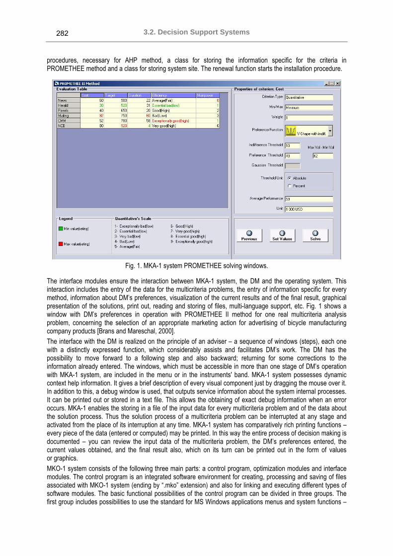
3.2. Decision Support Systems
282
procedures, necessary for AHP method, a class for storing the information specific for the criteria in PROMETHEE method and a class for storing system site. The renewal function starts the installation procedure.
Fig. 1. MKA-1 system PROMETHEE solving windows.
The interface modules ensure the interaction between MKA-1 system, the DM and the operating system. This interaction includes the entry of the data for the multicriteria problems, the entry of information specific for every method, information about DM’s preferences, visualization of the current results and of the final result, graphical presentation of the solutions, print out, reading and storing of files, multi-language support, etc. Fig. 1 shows a window with DM’s preferences in operation with PROMETHEE II method for one real multicriteria analysis problem, concerning the selection of an appropriate marketing action for advertising of bicycle manufacturing company products [Brans and Mareschal, 2000]. The interface with the DM is realized on the principle of an adviser – a sequence of windows (steps), each one with a distinctly expressed function, which considerably assists and facilitates DM’s work. The DM has the possibility to move forward to a following step and also backward; returning for some corrections to the information already entered. The windows, which must be accessible in more than one stage of DM’s operation with MKA-1 system, are included in the menu or in the instruments' band. MKA-1 system possesses dynamic context help information. It gives a brief description of every visual component just by dragging the mouse over it. In addition to this, a debug window is used, that outputs service information about the system internal processes. It can be printed out or stored in a text file. This allows the obtaining of exact debug information when an error occurs. MKA-1 enables the storing in a file of the input data for every multicriteria problem and of the data about the solution process. Thus the solution process of a multicriteria problem can be interrupted at any stage and activated from the place of its interruption at any time. MKA-1 system has comparatively rich printing functions – every piece of the data (entered or computed) may be printed. In this way the entire process of decision making is documented – you can review the input data of the multicriteria problem, the DM’s preferences entered, the current values obtained, and the final result also, which on its turn can be printed out in the form of values or graphics. MKO-1 system consists of the following three main parts: a control program, optimization modules and interface modules. The control program is an integrated software environment for creating, processing and saving of files associated with MKO-1 system (ending by “.mko” extension) and also for linking and executing different types of software modules. The basic functional possibilities of the control program can be divided in three groups. The first group includes possibilities to use the standard for MS Windows applications menus and system functions –

KDS 2005 Section 3: Decision Making
283
“File”, “Edit”, “View”, “Window”, “Help” and others in system own environment. The second group of control program facilities includes the control of the interaction between the modules realizing: creating, modification and saving of “.mko” files associated with MKO-1 system, which contain input data and data concerning the process and the results from solving multicriteria linear and linear integer problems; interactive solution of the multicriteria linear and linear integer problems which have been entered; localization and identification of the errors occurring during the system operation. The third group of the functional features of the control program includes possibilities for visualization of important information concerning the DM and the system operation as a whole. The optimization modules realize three classifications oriented interactive algorithms GAMMA-L, GAMMA-I1 and GAMMA-I2, and also exact and approximate single-criterion algorithms solving problems of the linear and linear integer programming. The interface modules realize the dialogue between the DM and MKO-1 system during the entry and correction of the input data necessary for the multicriteria problems during the interactive process of these problems solution, and also for the dynamic visualization of the main parameters of the process. An editing module serves to enter, alter and store the descriptions of the criteria, of the constraints, and also of the type and bounds of variables' alteration. Another interface module enables the setting of DM’s local preferences for alteration in the values of the separate criteria. A third interface module realizes two types of graphic presentation of the information about the values of the criteria at different steps and the possibilities for comparison. Dynamic Help is provided, which outputs specific information about the purpose and way of use of the fields and radio buttons in a separate window.
Fig. 2 MKO-1 Solving

3.2. Decision Support Systems
284
MKO-1 system is working under MS Windows. It can be added to Programs group and/or with a Desktop icon, from where it is started. The system registers the “.mko” extension and associates it. Thus at double clicking on a valid “.mko” file, the system will be started and this file will be loaded. There is a menu in the main window with the standard for MS Windows drop-down menus and commands. With their help, the operation of a new file is started or an existing “.mko” file is loaded and the operation may continue with the information stored in it. The entry and correction of the problem criteria and constraints is realized in “MKO-1 Editor” window. Every criterion and every constraint is entered separately in the respective text field for edition. Syntax check is accomplished when they are added to the data already entered. The syntax accepted is similar to the mathematical record of this class of optimization problems. The type of the optimum looked for is entered first – “min” or “max”. After that, the digital coefficient with its sign is entered, followed by the variable name it refers to. The variables names can be an arbitrary set of letters and numbers. Each one of these elements is separated by a space. The constraints have similar syntax – digital coefficients and variables names are successively entered. The type of the constraints is defined by some of the symbols “<=”, “>=” or “=”. By double clicking on the constraint or criterion already entered, they are transferred to the editing field again, if subsequent corrections are necessary. The interactive problems' solution is realized in “MKO-1 Solving” window. “MKO-1 Solving” window is divided into several zones (Fig. 2). Its upper part contains a band with buttons that realize the main functions of the process for interactive solution of multicriteria linear and linear integer problems. The next field of “MKO-1 Solver” window contains radio buttons for setup of the MKO-1 solution looked for: continuous, integer, approximate integer, the closest integer, as well as weak Pareto optimal or Pareto optimal. Below them information is found about the time of the system operation for the current problem in seconds, the number of the step being currently considered and the total number of the executed steps. Two text fields follow. The first one outputs successively the values of the criteria obtained at the current step. It is an operating field where DM’s preferences relating to the search of the next solution are set. After marking each one of the criteria, a context field is opened with the help of the mouse right button, where the DM sets the desired alteration in the value of this criterion at a following iteration. In case the selection is connected with the necessity to enter a particular value, MKO-1 system opens an additional dialogue window and waits for the entry of the corresponding digital information. When interactive algorithms are used for multicriteria optimization problems solving, it is an advantage to present information not only about the last solution found, but also about the process of search, about all the previous steps. Given that some significant solutions are made on the basis of these results, it is important for the DM to be able to “testify” how he has reached this solution. That is why the information about the interactive process of multicriteria optimization problem considered, which consists of the problem input data, the solutions obtained at each step, the preferences set by the DM for a new search and the constructed scalarizing problems, saved in *.mko files associated with MKO-1 system serve not only for restarting an interrupted solution process, but also for documentation. ”Print” command from the main menu can be used for selective print of the type of information chosen by the DM.
Conclusion
MultiDecision-1 system is designed to support DMs in solving different multicriteria analysis and multicriteria optimization problems. MKA-1 system is designed to support the DM in modelling and solving problems of multicriteria ranking and multicriteria choice. The integrating of three different types of methods expands DM’s possibilities to set his/her preferences about the quality of the most preferred solution. MKO-1 system is designed to model and solve linear and linear integer problems of multicriteria optimization. The interactive classification-oriented algorithm included in the system offers the DMs wide possibilities to set his/her preferences about the qualities of the most preferred solution. The user-friendly interface of MKA-1 system and MKO-1 system facilitates the operation of DMs with different qualification level relating to the analysis and the optimization methods and software tools. MKA-1 and MKO-1 systems can be used for the purposes of education and for experimental and research problems solving as well.

KDS 2005 Section 3: Decision Making
285
Bibliography [Benayoun, et al.,1971] R. Benayoun, J. Montgolfier, J. Tergny, O. .Laritchev. Linear Programming with Multiple Objective
Functions: Step Method (STEM). Mathematical Programming, 1, 136-375. 1971 [Brans and Mareschal, 1990] J. P. Brans, and B. Mareschal. The Promethee Methods for MCDM: the Promcale, Gaia and
Bankadviser Software. In: Readings in Multiple Criteria Decision Aid. Ed. C. A.. Bana e Costa. Springer-Verlag, Berlin, 216-252. 1990.
[Brans and Mareschal, 1994] J. P. Brans, and B. Mareschal. The PROMCALC & GAIA Decision Support System for Multicriteria Decision Aid. Decision Support System, 12, 297-310. 1994.
[Brans and Mareschal, 2000] J. P. Brans, and B. Mareschal. How to Decide with PROMETHEE? http://www.visualdecision. com. 2000.
[Gardiner and Vanderpooten, 1997] L. R Gardiner and D. Vanderpooten. Interactive Multiple Criteria Procedures: Some Reflections. In: Multicriteria Analysis. Ed. J. Climaco. Springer-Verlag, Berlin, 290-301. 1997.
[Jaszkiewicz and Slowinski, 1994] A. Jaszkiewicz and R. Slowinski. The Light Beam Search Over a Non-Dominated Surface of a Multiple-Objective Programming Problem, In: Multiple Criteria Decision Making. Eds G.H. Tzeng, H.F. Wang, U.P. Wen and P.L. Yu. Spinger-Verlag, Berlin, 87-99. 1994.
[Keeney and Raiffa, 1976] R. Keeney, and H. Raiffa. Decisions with Multiple Objectives, Preferences and Value Trade Offs. John Wiley & Sons. New York. 1976.
[Korhonen, 1988] P. Korhonen. A Visual Reference Direction Approach to Solving Discrete Multiple Criteria Problems. European Journal of Operational Research, 34, 152-159. 1988.
[Korhonen, 1987] P. Korhonen. VIG - A Visual Interactive Support System for Multiple Criteria Decision Making. Belgian Journal of Operations Research, Statistics and Computer Science 27(1), 3-15. 1987.
[Lewandowski and Wierzbicki, 1989] A. Lewandowski and A.P. Wierzbicki. Aspiration Based Decision Support Systems, Lecture Notes in Economics and Mathematical Systems, 331, Spinger – Verlag, Berlin. 1989.
[Miettinen, 1999] K. Miettinen. Nonlinear Multiobjective Optimization. Kluwer Academic Publishers, Boston. 1999. [Miettinen and Makela, 2000] K. Miettinen and M. Makela. Interactive Multiobjective Optimization System WWW-NIMBUS on
the Internet. Computer and Operation Research, 27, 709-723. 2000. [Mustajoki and Hamaiainen, 2000] J. Mustajoki and R. P. Hamalainen. Web-HIPRE: Global Decision Support by Value Tree
and AHP Analysis. INFOR, 38, 208-220. 2000. [Narula et al., 2003] S.C.Narula, V. Vassilev, K. Genova, M. Vassileva. A Partition-Based Interactive Method to Solve
Discrete Multicriteria Choice Problems, Cybernetics and Information Technologies, 2, 55-66. 2003. [Narula and Vassilev, 2003] S. C. Narula and V. Vassilev. An Interactive Algorithm for Solving Multiple Objective Integer
Linear Programming Problems. European Journal of Operational Research, 79, 443-450. 1994. [Nemhauser and Wolsey, 1988] G. L Nemhauser and L. Wolsey. Integer and Combinatorial Optimization. Wiley,
New York. 1988. [Ogryczak et al., 1992] W. Ogryczak, K. Stuchinski, K. Zorychta. DINAS: A Computer-Assisted Analysis System for
Multiobjective Transhipment Problems with Facility Location. Computers and Operations Research 19, 637-648. 1992. [Osyczka, 1988] A. Osyczka. Computer Aided Multicriterion Optimization System. In: Discretization Methods and Structural
Optimization – Procedures and Applications. Eds. H. A. Eschenauer and G. Thierauf. Spinger-Verlag. 263-270. 1988. [Parsons, 2002] J. Parsons. Agland Decision Tool: A Multicriteria Decision Support System for Agricultural Property, iEMSs
2002, Integrated Assessment and Decision Support, Proceedings, Volume 3, 181-187, http://www.iemss.org/iemss2002/. [Peterson, 1994] C. R. Peterson. HIVIEW – Rate and Weight to Evaluate Options. OR/MS Today, April. 1994. [Roy, 1991] B. Roy. The Outranking Approach and the Foundations of ELECTRE Methods. Theory and decision, 31,
49-73. 1991. [Saaty, 1980] T. S. Saaty. The Analytic Hierarchy Process. McGraw-Hill, New York. 1980. [Saaty, 1994] T. S. Saaty. Highlights and Critical points in the Theory and Application of the Analytic Hierarchy Process.
European Journal of Operational Research, 74, 426-447. 1994. [Sun and Steuer, 1996] M. Sun and R. Steuer. InterQuad: An Interactive Quad Free Based Procedure for Solving the
Discrete Alternative Multiple Criteria Problem. European Journal of Operational Research, 89, 462-472. 1996. [Vansnick, 1986] J. C. Vansnick. On the Problem of Weights in Multiple Criteria Decision Making (the noncompensatory
approach). European Journal of Operational Research, 24, 288-294. 1986. [Vassilev et al., 1993] V. Vassilev, A. Atanassov, V. Sgurev, M. Kichovitch, A. Deianov, L. Kirilov., Software Tools for Multi-
Criteria Programming. In: User-Oriented Methodology and Techniques of Decision Analysis and Support. Eds. J. Wessels and A. Wierzbicki. Spinger- Verlag, Berlin, 247-257. 1993.
[Vassilev et al., 1997] V. Vassilev, S. Narula, P. Vladimirov, V. Djambov. MOIP: A DSS for Multiple Objective Integer Programming Problems. In: Multicriteria Analysis, Ed. J. Climaco. Springer-Verlag, Berlin, 259-268. 1997.

3.2. Decision Support Systems
286
[Vassilev et al., 2003] V. Vassilev, K. Genova, M. Vassileva, S. Narula. Classification-Based Method of Linear Multicriteria Optimization. International Journal on Information Theories and Aplications, vol.10, 3, 266-270. 2003.
[Vassileva et al., 2001] M. Vassileva, K. Genova, V. Vassilev, A Classification based Interactive Algorithm of Multicriteria Linear Integer Programming. Cybernetics and Information Technologies, 1, 5 – 20. 2001.
[Vassileva, 2004] M. Vassileva. A Learning-oriented Method of Linear Mixed Integer Multicriteria Optimization. Cybernetic and Information Technologies, 4, No 1, 13-25. 2004.
[Vincke, 1992] P. Vincke. Multicriteria Decision-Aid. John Wiley & Sons, New York. 1992. [Von Winterfeldt and Edwards, 1986] D. Von Winterfeldt and W. Edwards. Decision Analysis and Behavioral Research,
Cambridge University Press, London. 1986. [Wierzbicki, 1980] A. P. Wierzbicki. The Use of Reference Objectives in Multiobjective Optimization. In: Multiple Criteria
Decision Making Theory and Applications. Lecture Notes in Economics and Mathematical Systems 177, Eds. G. Fandel and T. Gal. Spinger-Verlag, Berlin, 468-486. 1980.
Author information
Vassil Vassilev – Institute of Information Technologies, BAS, Acad. G. Bonchev St., bl. 29A, Sofia 1113, Bulgaria; e-mail: [email protected] Krasimira Genova – Institute of Information Technologies, BAS, Acad. G. Bonchev St., bl. 29A, Sofia 1113, Bulgaria; e-mail: [email protected] Mariyana Vassileva – Institute of Information Technologies, BAS, Acad. G. Bonchev St., bl. 29A, Sofia 1113, Bulgaria; e-mail: [email protected]
RECOGNITION ON FINITE SET OF EVENTS: BAYESIAN ANALYSIS OF STATISTICAL REGULARITY AND CLASSIFICATION TREE PRUNING
Vladimir B. Berikov
Abstract: The problem of recognition on finite set of events is considered. The statistical regularity of decision functions for this problem is studied within the Bayesian approach. The results are applied in pruning of classification trees.
Keywords: statistical regularity, Bayesian learning, classification tree pruning.
Introduction
In the theory of statistical pattern recognition, an important problem is the statistical regularity of decision functions. This problem arises from the need to find a decision function having good generalization ability provided that the probability distribution is unknown, and learning sample has limited size. A number of different approaches to the solution of the problem can be formulated: experimental approach (based on one-hold-out procedure and its modifications), probabilistic approach (based on preliminary evaluation of distribution law), the approach based on principles of multivariate statistical analysis, statistical learning theory, algorithmic approach, Bayesian learning theory. Experimental approach is extremely labor-consuming; within the framework of the probabilistic approach asymptotic quality evaluations are received basically. In the next approaches, the finiteness of sample is taken into account; however multivariate analysis requires rather bounded classes of distributions and types of decision functions. Statistical and algorithmic approaches are oriented basically on worst-case analysis. So the received performance estimates are powerfully lowered. Within the Bayesian approach, the average-case estimates are received, which, as was shown in [1], are more fit to volumes of samples available in practical tasks.

KDS 2005 Section 3: Decision Making
287
Regrettably, the expressions, received within the Bayesian approach, as a rule, have unclosed form, are cumbersome and labor-consuming in calculating. Thus, a problem of finding more effectively calculated evaluations (possibly, approximate) is actual. These evaluations are to be applied as a quality criterion in a learning step at the building of decision functions from the sample. The study of statistical regularity undertaken in given work has the following particularities. Firstly, the Bayesian approach is applied. Secondly, the narrower class of recognition problems – the problems of recognition on finite set of events is considered. This type of problems is most suitable for analytical studies. On the other hand, the results can be extended on broadly used classes of decision functions – logical decision functions and decision trees.
Main Definitions
Let us consider a pattern recognition problem with K≥2 classes, input features X1,X2,…,Xn and output feature Y with domain DY=1,…,K. Denote Di as a set of values of feature Xi, i=1,…,n. Suppose that the examples from
general sample are extracted by chance, therefore the features Y, Xi are casual. A function1
n
i Yi
f : D D=
→∏ is
called the decision function. A special kind of the decision function is a decision tree T. Consider binary trees: each node Tt∈ of the tree can be branched out into two branches. Each internal node is labeled with a feature and each branch corresponds to a subdomain of definition of that feature. To each leaf we assigned the majority class of all examples of this leaf. Decision function is built by the random sample of observations of X and Y («learning» sample). Let learning sample be divided on two parts. The first part is used to design decision tree T, and the second part to prune it. Let prT be a pruned decision tree. During the pruning process, one or more nodes of T can be pruned. By numbering the leaves of a tree, we can reduce the problem to one feature X. The values of this feature are coded by numbers 1,…,j,…, M, where M is number of leaves. Let i
jp be the probability of joint event “X=j,Y=i”. Denote
a priory probability of the i-th class as pi. It is evident that Σipi=1, Σjpij=pi. Let N be sample size, ijn be a
frequency of falling the observations of i-th class into the j-th cell. Denote )n,...,n,n,...,n,n(s KM
K 121
21
11= . Let us
consider the family of models of multinomial distributions with a set of parameters θΘ = , where )p,...,p,p,...,p,p( K
MK 1
2121
11θ = , ,p,p
j,i
ij
ij ∑ =≥ 10 K...i,M...j 11 == . Let N~ be a number of errors on
learning sample for the given decision function. The random vector of frequencies S belongs to the multinomial distribution with parameter vectorθ . In applied problems of recognition a vector θ is usually unknown. We use the Bayesian approach: suppose that random vector Θ = )P,...,P,P,...,P( K
MK 1
211
1 with known priory distribution )(θp is defined on the set of parameters. In the given work the case of uniform density constp =)(θ is considered. This assumption is defensible if a priory vagueness in choice of model is available. Let Y=f(X) be a decision function which has been found on sample s with the help of some deterministic algorithm. The probability of misclassification for this function equals to ∑−=
j
)j(fjf P)(P 1Θ .
Bayesian Estimate of Decision Function Performance and Decision Tree Pruning
The mean misclassification probability for decision function f is denoted as )(EPP fs,f Θ= .
Proposition 1:KMN
M)K(N~P s,f +−+
=1 .
The value Pf,s will be called the Bayes estimate of misclassification probability for decision function f and sample s.

3.2. Decision Support Systems
288
Proposition 2. The variance of misclassification probability equals: 1
1++
−=
KMN)P(P
VP s,fs,fs,f .
The proofs are given in [2]. The mean and variance, Pf,s and VPF,s, can be used for calculation of tolerance interval for the value of misclassification probability [2]. Let us suppose that there is an algorithm which can grow decision tree for classification of observations from first part of the sample. The parameters of the algorithm should be chosen in such a way to get a large number of leaves in the tree. Next, we classify the examples from the second part of the sample to define how many examples of each class are assigned to each node. Consider arbitrary subtree T of the initial tree (T and initial tree have the same root). The set of leaves of T can be considered as a set of values of feature Х. The vector of the observed frequencies for all leaves can be considered as a vector of frequencies s. Note that subtree T does not depend on the vector s, because the observations from pruning part are not participated in the tree building. For subtree T, we can compute the Bayesian estimate of misclassification probability PT,s. This value can be used as criterion of quality for subtree. An optimization of the criterion gives optimization of the tree complexity (the number of leaves become optimal). Let us suppose that vector θ is fixed, but unknown parameter vector. In this case, the Bayesian estimate of misclassification probability for decision function is the approximation of the true unknown generalization error. It is possible to show that the Bayes estimate is asymptotically unbiased. In the same time the empirical error estimate ( N
N~ ) is unbiased, however the variance of the Bayesian estimate is less than the variance of the empirical estimate. In this sense, the Bayes estimate is more stable.
Numeric Simulation
For numeric experiments the breast cancer database [3] was used. For decision tree building was used standard algorithm C4.5 [4]. The algorithm grows a large tree from learning sample. Then this tree is pruned by second part of learning sample. The “greedy” algorithm of optimal pruning variant search is applied. After the pruning, obtained decision tree is evaluated by test data set. Three different strategies of experiments were considered. 1. The data set is divided into three parts: for decision tree growing 50%, for pruning 30% and for testing 20%.
Standard reduced error pruning method (REP) [4] was used for pruning. 2. The data set divided in the same way as in first strategy. We used the Bayesian estimate of error probability
for pruning. 3. The data set is divided into two parts. The first one (80%) is used for decision tree growing and then for
pruning and the second one (20%) is used for testing. The Bayesian estimate is used for pruning. It is known that if growing and pruning sets coincide, the effect of overtraining arises. The purpose of this experiment is to study the behavior of the decisions in this situation.
All experiments were repeated 200 times. Before each experiment, the observations in data set were randomly mixed. The following results of computer modelling were obtained. For first and second strategy, the errors on test sample coincide (0.022 at average). For third strategy, REP could not prune the tree; the average error on test samples for the Bayesian pruning algorithm was 0,067. For the next experiment, artificially generated data table was used. This table was unbalanced: the frequencies of classes differ in a large degree (fist class represents 5% and second 95% of sample size of 1000 examples). The 10-fold cross-validation technique was applied for quality estimation. It turned out that the proposed method accuracy was 7% better than the accuracy of REP.
Conclusion
Within the framework of the Bayesian learning theory, the problem of statistical regularity of decision functions for recognition on finite set of events was considered. It was shown that the obtained results can be applied for classification tree pruning. Numeric experiments showed that the Bayesian pruning has at least the same efficiency or better than standard reduced error pruning, and at the same time it is more resistant to overtraining.

KDS 2005 Section 3: Decision Making
289
Acknowledgements
This work was supported by the Russian Foundation of Basic Research, grant 04-01-00858a
Bibliography
[1] Lbov, G.S., Startseva, N.G., About statistical robustness of decision functions in pattern recognition problems. Pattern Recognition and Image Analysis, 1994. Vol 4. No.3. pp.97-106.
[2] Berikov V.B., Litvinenko A.G. The influence of prior knowledge on the expected performance of a classifier. Pattern Recognition Letters, Vol. 24/15, 2003, pp. 2537-2548.
[3] UCI Machine Learning Database Repository. http://www.ics.uci.edu/~mlearn/ MLRepository.html [4] Quinlan, J.R. C4.5: Programs for Machine Learning. Morgen Kaufmann, San Mateo, CA, 1989.
Author's Information
Vladimir Berikov – Sobolev Institute of Mathematics SD RAS, Koptyug pr.4, Novosibirsk, Russia, 630090; e–mail: [email protected]
DECISION FOREST VERSUS DECISION TREE
Vladimir Donskoy, Yuliya Dyulicheva
Abstract: A research and improvement of learning and recognition algorithms based on building up binary decision trees (BDT); to working out the rules for binary decision trees pruning on the basis of conjunctive regularities evaluation; to creating consistent decision tree family synthesis procedure (i.e. the empirical decision forest synthesis algorithm) and pruned decision trees family correction methods as a set of heuristic procedures for decision making are considered.
Keywords: empirical decision forest, conjunctive regularity, decision tree pruning criterion, overfitting, VCD of decision rules class
Introduction
A decision forest versus a decision tree problem is to compare the advantages and disadvantages of two inductive models. In this paper we discuss the following question. What are the possibilities that make the empirical decision forest more effective versus the decision tree? The advantages of the proposed empirical decision forest versus the decision tree are grounded a more effective mechanism of regularities reveal from data; the maximal employment possibility of all initial training information; insignificant complication of the decision making procedure; a possibility of accurate fitting on the correct classification of much more training objects number; insignificant complication of the decision rules class generated from the empirical decision forest compared to the decision rules class generated from the single decision tree. It is known that increase of the decision tree structure complexity facilitates to obtaining of a correct recognition algorithm according to the initial training sample, i.e. precisely fitted on the training sample. If the decision tree structure complexity is not restricted, it is always possible to build up the non-unique precisely fitted on the training sample (correct according to the initial training sample) learning algorithm with the decision tree structure. Based on Vapnik-Chervonenkis’ statistical learning theory the decisions (the required recognition algorithms) will be found in the class of unbounded capacity that one makes a learning ability with the given guaranteed accuracy

3.2. Decision Support Systems
290
impossible. A theoretically grounded undesirability of the decision tree structure complication in the synthesis (learning) process finds a confirmation in an overfitting effect discovered in the numerous experiments. The decision trees complexity is naturally restricted based on the decision trees branches pruning or the leaves number reduction. The well-known approaches [Breiman, 2001; Breslow, Aha, 1997; Frank, 2000; Ho, 1995; Ho, 1998; Malerba, Esposito, Semeraro, 1996; Murphy, Pazzani, 1994; Schaffer, 1993] aimed to the restriction of the decision trees structure complexity were dedicated to a compromise searching for the redundant complication of the decision tree structure and the obtaining of quality evaluation of the constructed decision tree as high as possible. Saving the ability to the classification quality increase on control the pruning usually leads to the incorrect decision tree synthesis according to the training sample. However pruning process can lead to the classification rules errors according to the reliable training sample in case of the incorrect decision tree precisely fitted on the sample. It is arisen a following new “subtle” problem statement. Is it possible (and if possible then how) to obtain the decrease of the decision tree structure complexity saving the requirement of its correction according to the reliable training sample? Exactly in this context the investigations were carried out directed to the dilemma resolving: to fit the decision tree precisely on the reliable training sample or to restrict the decision rules complexity for saving the high capability to generalization of the initial training sample properties on the basis of the empirical induction principle.
1. Decision Trees Pruning Criterion Reasoning
Since it is undesirable to complicate the decision trees in connection with their overfitting on the training sample, the decision tree complexity ground problem is becoming especially important. For binary decision tree structure this problem is connected with decision tree pruning. Unfortunately most acknowledged decision tree pruning algorithms have no any grounding. We propose a grounded decision tree pruning strategy on the basis of a conjunctive regularity notion. Let mnT be an initial training sample that is given as an empirical training table, where m be the objects number or the table’s rows number; n be the attributes number or the table’s columns number and a goal column is not separated from the training table columns. Let lmnT be a standard training table with separated goal column where l the number of classes and the goal column consists of the classes’ labels. Suppose that the classes’ label values are Boolean and if ( ) lmnnj Txxxx ∈= ~,...,,...,1 then 1,0∈ix , ni ,1= .
Whereas the training sample size is bounded compared to a universe size the regularities reveal process from the empirical training table has a hypothesis character. We specify a notion of a conjunctive regularity of rank r according to the training table mnT .
Definition 1.1 A conjunction of rank r ri
r
iiiiir xxxKσσσ
&&& 22
11
K= is called the conjunctive regularity
of rank r according to the empirical training table mnT if there exists r columns with numbers riii ,,, 21 K and column with number riiik ,,, 21 K∉ such that the variable kx takes on the same value σγ ~ for all rows mnTx ∈~ with a property
rr iiiiii xxx σσσ === ,,,2211K . In addition the sets
1,,,:~2211
TTxxxx mniiiiii rr=∩=== σσσ K and 1\ TTmn are not empty.
Let nmBDT ,,µ be a binary decision tree (BDT) with µ leaves being built up according to the training table
mnT . Based on the conjunctive regularity notion BDT defines the conjunctive regularities set
µrrr KKK ,,,21K ensuring the decisions derivation. These conjunctions are orthogonal by pairs since they
correspond to different branches of the decision tree.

KDS 2005 Section 3: Decision Making
291
Theorem 1.1 A probability ( )nmPBDT ,,µ of a random derivation of property kx for an arbitrary object ( )nkk xxxxxx ,,,,,,~
1121 KK +−= being uniformly selected from Boolean vectors set with length n-1 based on the correct binary decision tree with µ leaves being built up according to the empirical training table is evaluated by the following inequality
( ) ( ) ⎟⎠⎞⎜
⎝⎛ −+−
=−∑<
jrjj
rmrnj
jBDT CrnnmP
2
12,,
µµ (1.1)
where µrrr ,,, 21 K are the decision tree branches’ ranks.
Remark 1.1 If the decision tree being built up according to the standard training table with n Boolean attributes then the probability of the random finding of this decision tree is evaluated by the following inequality
( )⎟⎠⎞⎜
⎝⎛ −+−
=∑<
jjj
rrmrn
jBDT CnmP
2
1
* 2,,µ
µ (1.2),
where µrrr ,,, 21 K be the ranks of conjunctions that correspond to BDT’s branches; and µ be the number of leaves. The conjunctive regularity of rank r defines an implicative rule of the decision making
σγσσσ ~22
11
&&& kiii xxxx ri
r
ii →⎟⎠⎞
⎜⎝⎛ K (1.3), i.e. this rule allows to compute a value of the goal variable kx if
a vector ( )nxxxx ,,,~21 K= belongs to the interval
rKN corresponding to the conjunction rK from the left part of the implicative rule (1.3). Based on Kolmogorov’ approach which considers regularity as non-randomness, the remark 1.1 result and the implicative rule (1.3) a “non-random” decision will be derived from the training sample with probability less than
⎟⎠⎞⎜
⎝⎛ −+−
=∑−
jrjj
rmrn
jC
2
121
µ.
Let nmD ,,µ be a class of all possible correct decision trees with µ leaves being built up according to the
standard empirical training table lmnT . On the basis of evaluation (1.2) it is defined a quality functional RD nm →,,: µϕ as follows
( )⎟⎟⎟
⎠
⎞
⎜⎜⎜
⎝
⎛=
⎟⎠⎞⎜
⎝⎛ −+−
≤≤
jrjj
rmrn
jCd
2
12max
µϕ (1.4)
The quality functional ( )dϕ is the evaluation of “worse” case, i.e. decision making is accomplished the decision tree branch of maximal rank. It is grounded by the following lemma.
Lemma 1.1 A value ( ) ( )rrmrnCrmnh 22,, −+−= is growing monotonously along with the growth of BDT
branches’ rank r, if 2≥r and 1+≥ rn . Hence it is naturally arisen the quality functional minimization problem. The result of lemma 1.2 is the optimal decision tree structure.
Lemma 1.2 The quality functional ( )dϕ minimum defined on the set nmD ,,µ of the binary decision trees
( )⎟⎟⎟
⎠
⎞
⎜⎜⎜
⎝
⎛=
⎟⎠⎞⎜
⎝⎛ −+−
≤≤∈
jrjj
nm
rmrn
jDdCd
2
1* 2maxmin
,, µµϕ

3.2. Decision Support Systems
292
is reached if Nkk ∈= ,2µ , i.e. *d be the complete decision tree or if k2≠µ and the decision tree *d
satisfies to condition 1max1
≤−≤<≤
qjqj
rrµ
, where µrrr ,,, 21 K be conjunctions’ ranks corresponding to the
branches of BDT *d .
Definition 1.2 The binary decision tree is named uniform if its branches’ rank differ at most one.
Theorem 1.2 The uniform trees have the minimum evaluation (1.4) of the probability of random decision derivation in the empirical decision trees class nmD ,,µ .
Theorem 1.2 result is the theoretical grounding of the decision tree branches pruning that maximize the quality functional value (1.4), i.e. the decision tree branches criterion. The pruning process directs to the decision tree structure simplification for obtaining the decision tree structure which is as close as possible to the uniform decision tree structure.
2. Decision Forest and Decision Rules Synthesis Algorithms
A new proposed synthesis algorithm of an empirical decision forest inductive model is the prepruning strategy with a special mechanism of the attributes review. The empirical decision forest (EDF) synthesis is aimed at searching for such forest’s branch system that would give a correct classification for all objects of the no contradictory training sample based on the conjunctive regularity of the predetermined admissible rank. Definition 2.1 An interval
jKN corresponding to the decision tree branch with rank rrj > (r be the
predetermined admissible rank) is named a binary decision tree rejection set. It is supposed that the empirical binary decision tree rejection set contains objects influencing on the binary decision tree structure complication, i.e. the leaves number increase or the branches’ ranks increase. Definition 2.2 A pointer on the decision tree 2d root node placed in every leaf of the decision tree 1d corresponding to the rejection set is called a reference 12c from the decision tree 1d to the decision tree 2d .
Definition 2.3 An ordered set of the empirical decision trees ( )qr dddD ,,, 21 K= with the references
qqccc 12312 ,,, −K is named the empirical decision forest. Define two types of the empirical decision forest depending on the capability to recognize correctly objects from the initial training sample, i.e. the capability to fit precisely on the training sample without the overfitting effect appearance. Definition 2.4 The empirical decision forest is called r-correct according to the standard training table lmnT if all its trees ( )qddd ,,, 21 K have branches’ rank values no more than predetermined admissible rank r value, the
last in order decision tree qd has no branches corresponding to the rejection sets and decision rules being generated from the empirical decision forest allow to compute precisely the classes’ label for all objects from the training table lmnT . The empirical decision forest is called r-incorrect according to the training table lmnT if there exists at least one training object incorrectly classified by the empirical decision forest. The main idea of the decision rules synthesis so called decision making procedure with references switching based on the empirical decision forest that is made up by the decision tree family ( )qddd ,,, 21 K is as follows.
In case there is no conjunctive regularity in 1d decision tree with the rank admissible for the classification of the object that is not a part of training, its classification is to be performed by another decision tree 2d . If there is no conjunctive regularity in 1d decision tree with the predetermined admissible rank, the object is to be “transferred” to the next decision tree that is defined by the order of the empirical decision forest tree synthesis.
The synthesis algorithm of the r-pruned empirical decision forest

KDS 2005 Section 3: Decision Making
293
10. The decision tree 1d is built up based on one of the synthesis strategies proposed in [Донской В.И., Башта А.И., 1992; Cremilleux, Robert, 2000]. If it is correct according to the standard training table lmnT and its branches’ ranks do not exceed the predetermined admissible rank r then the empirical decision forest synthesis is complete and the algorithm result is the forest composed of one decision tree ( )1dDr = . Otherwise go to 20.
20. Let nxxxX ,,, 21 K= be an initial attributes set, 1dX be an attributes set used in the first decision tree
1d synthesis process. If there exists at least one branch of the first decision tree 1d which rank value exceeds the predetermined admissible rank value then this branch is pruned and the reference from the first decision tree
1d to the second decision tree 2d is placed. The decision tree branch pruning is to replace internal node with number (r+1) by a special terminal node named the reference. The rejection set is defined as interval corresponding to the decision tree pruned branch. The decision tree with the references, i.e. not empty rejection sets, is named r-pruned decision tree. The references to the decision tree 2d are placed for all decision tree 1d rejection sets. The decision tree 2d is built up first of all on the attributes from
1\ dXX set if the set is not
empty and it has enough training objects for the decision tree 2d synthesis. If =1
\ dXX Ø then the attributes
choice order is changed compared to the decision tree 1d attributes choice order. Let 1jKN be the decision
tree 1d united rejection set; 12 jKmn NTT ∩= l be a set of the training objects from different classes that
belong to the rejection set 1jKN . The decision tree 2d is built up according to the training table 2T and then is
rebuilt up according to the training table 2\ TTmnl . The result of two algorithm steps is as a matter of fact the r-incorrect decision tree 2d and therefore the r-incorrect empirical decision forest ( )21, ddDr = . If the r-correct empirical decision forest is obtained then the decision forest synthesis algorithm is complete, otherwise it is necessary to construct a decision tree 3d with reiteration all main stages of step 20 .
Picture 2.1 The main stages of the empirical decision forest synthesis algorithm
. . .
first decision tree synthesis according to
lmnT
Pruning and first decision tree rejection set (Rejection Set1)
creation
second decision tree synthesis according to Rejection Set1
objects and
1\ dXX attributes
second decision tree “completion” according to \lmnT Rejection
Set1 training objects
pruning and the total rejection set creation (Rejection Set1 and Rejection
Set2) based on first and second decision

3.2. Decision Support Systems
294
The possible stopping criteria of the empirical decision forest synthesis process are 1. r-correct empirical decision forest has been built up; 2. the attempts of new decision trees synthesis have been performed more than given repeats number; 3. Computer resources needed for decision forest trees location have been limited.
The picture 2.1 illustrates the main stages of the empirical decision forest synthesis process.
The decision trees as components of the constructed empirical decision forest contain two types of the terminal nodes: the terminal node with class label typically named leaf and the terminal node corresponding to the rejection set named cut (pruned node) or reference. The empirical decision forest correctness condition will be met if some conjunctive regularity of the predetermined admissible rank is found for each object from the noncontradictory training table. Theorem 2.1 The r-correct empirical decision forest according to the training table lmnT exists if and only if
there exists the interval rxN~ with rank value that does not exceed the predetermined admissible rank value such
that rxNx ~~∈ and the set lmn
rx TN ∩~ contains the training objects belonging to only one class.
The decision rules (disjunctive normal forms) synthesis algorithm generated from the empirical decision forest
10. The conjunctions corresponding to the all branches of first decision tree as forest component with classes’ label are “written out” and the disjunctive normal form ( )jD ω1 is formed for each class jω , l,1=j as the logical description of the class with number j .
i0. Let ( )jiD ω1− , 1−iR have been built up (let 1,1 ≠− iRi be the rejection sets intersection as the logical
description of all 1−i decision trees generated from the empirical decision forest). For the decision tree id the logical description construction for class with number j is given as recursive procedure
( ) ( ) ( )( )jiijiji DRDD ωωω ∧∨= −− 11 .
The decision derived from the empirical decision forest according to the recognition algorithm with references switching out is made on the basis of only one conjunction of the bounded rank but possibly in condition when all previous decision trees from the empirical decision forest are rejected to decide. The main property of each such conjunction is its correctness according to the training table lmnT , i.e. it is implemented only for one class objects. The appropriateness of further recognition rules complication for building up decision making correction procedures is grounded on the basis of VCD evaluations for recognitions class algorithms that are defined by the empirical decision forest, i.e. the decision trees family using special pruning procedure. Compared VCD evaluation for decision rules class generated from the decision tree with Simon’s bounded rank [Simon, 1991; Дюличева Ю.Ю., 2003] ( ) ( )r
n nrDTVCD Θ= with VCD evaluation for the decision rules class generated from the decision tree with bounded leaves number ( )( ) ( )nnBDTVCD 2log, Θ=µ it is valid to say that the decision tree structure optimization on the basis of leaves number is more effective than the decision tree structure optimization on the basis of Simon’s bounded rank. The conclusion novelty concludes in grounding of the decision tree structure optimization on the leaves number according to Vapnik-Chervonenkis’ theory. The evaluations of VCD of the decision rules class generating from the empirical decision forest were derived:
( ) ( )( )2
loglog,,,log,max 222qqnqrqrnBDFVCDnq µµµµµ −<<
( )( ) ( )nqrnBDFVCD 2log,,, Θ=µ where constqr =,,µ , ∞→n The evaluations show that the recognition algorithms class based on the empirical decision forest synthesis has the same degree of complexity as the class of algorithms that are based on the single decision tree use and is equal to ( )n2logΘ where n be the attributes space dimension.

KDS 2005 Section 3: Decision Making
295
3. Decision Forest Based Technology. Some Experiments Result
The worked out program software so called Forest Based Learning (FBL) system is intended to solve the training and recognition problems based on the single decision tree and the empirical decision forest synthesis according to the same attributes choice principle with using the new decision tree branches pruning strategy. FBL system allows users to compare the quality characteristics of the single decision tree and the correct empirical decision forest. In particular it is possible to obtain information about the number of control objects that are correctly classified by the single decision tree and the empirical decision forest, the number of objects in the rejection sets formed in each synthesis stage of the decision tree as next component of the empirical decision forest, the number of leaves in each decision tree as forest’s component, the decision tree branches’ rank values that lead to “error” in recognition process, i.e. the redundant branches’ rank values and to obtain the logical description of classes as disjunctive normal forms. The table demonstrates that 6-correct (the branches’ ranks are not more 6) empirical decision forest facilitates to significant decrease of the recognition errors percent compared to the single correct BDT (the average branches’ ranks are not more than 8 and the average number of leaves are 20).
the average errors percent on the control sample correct BDT 6,1
EDF with rank 5 6,18 EDF with rank 6 5,5
The practical confirmation of the theoretically grounded results was obtained in the recognition problem solving process of the pathogenic vibrios and aeromonads that provoke the different gastrointestinal sicknesses. The experiments that allow to evaluate the reliability of the constructed empirical decision forest were carried out on the training samples with size 310=m selected randomly and independently from real database of size 465. The correct decision tree and the r-correct empirical decision forest were built up according to these randomly selected training samples. In each such experiment BDT and EDF were evaluated on control set of size 55. The experiment were repeated n=100 times. As the experiments result such outcomes as events A, B, С were considered. Let A was the event that EDF performed less errors on control than BDT; B was the event that EDF and BDT performed equal number of errors on control; C was the event that BDT performed less error on control than EDF. The event A was appeared 24=Am times in 100 experiments; the event C was
appeared 5=Bm times in the same 100 experiments. The frequencies ( )An
mA ν= and ( )Bn
mB ν= were
corresponded to the probability evaluations ( )AP and ( )BP of the recognition accuracies on the arbitrary control set for EDF and BDT accordingly. Based on the criterion [Гмурман В.Е., 2001] a hypothesis 1H : ( ) ( )BPAP > was checked versus a competitive hypothesis 0H : ( ) ( )BPAP =
7,3111
≈
⎟⎠⎞
⎜⎝⎛ +⎟⎠⎞
⎜⎝⎛
++
−++
−=
nnnnmm
nnmm
nmnmUBABA
BAH
The evaluations ( ) 49,0221 =− α ; ( ) 49,0=Φ крU ; 32,2=крU ; Hкр UU =<= 7,332,2 (3.1) were obtained on the basis of the significance level 01,0=α . Based on the obtained inequality (3.1) the hypothesis
1H was taken up. Thus, it is valid to say that on the significance level 0.01 the empirical decision forest will make less recognition errors on control than the binary decision tree in average. The picture illustrates the synthesis fragment of the single correct decision tree and the correct empirical decision forest with branches’ rank 5 on the basis of Forest Based Learning Technology.

3.2. Decision Support Systems
296
Conclusion
The major results of the paper done are as follows. The probabilistic decision tree pruning criterion was worked out which applies to the branches with the number of internal nodes exceeding the predetermined admissible value of r rank. The grounding for the pruning as viewed as non-randomness of detecting r rank conjunctive regularity in the empirical training sample is suggested in the paper. The methods for building up a correct decision tree family so called empirical decision forest were worked out which offers a possibility for accurate fitting on the training sample, with the restriction applying to BDT rank branches being observed. The appropriateness of further complication of recognition rules for building up decision making correction procedures is grounded on the basis of VCD (with the decision rules complexity according to Vapnik-Chervonenkis theory [Вапник В.Н., 1979]) evaluation for recognition class algorithms that are defined by the binary decision tree with the pruning applying to the number of nodes. The algebraic correction model of the incorrect empirical decision trees family was worked out which gives way to more accurate classification [Журавлев, 1978, Донской В.И., 1986]. The software was created to implement the algorithms introduced in the paper, and experiments had been carried out with real data involved that justified the theoretical results reached. The procedural technique of pruned BDT correction so called empirical decision forest that is introduced in the paper enables one to achieve a much more recognition algorithm compared to the algorithms that are realized by the single correct BDTs. Along with that the EDF is still available for logical description of objects as disjunctive normal forms. The appropriateness of applying the empirical decision forest in modern intellectualized informational systems is justified by Forest Based Learning - the program realization that was tested and approved in the paper.
Bibliography [Вапник В.Н., 1979] Вапник В.Н. Восстановление зависимостей по эмпирическим данным. – М.: Наука, 1979. – 448 с. [Гмурман В.Е., 2001] Гмурман В.Е. Теория вероятностей и математическая статистика. – М.: Высшая школа, 2001. 479с. [Донской В.И., Дюличева Ю.Ю., 2002] Донской В.И., Дюличева Ю.Ю. Индуктивная модель r-корректного эмпирического
леса // Труды международной конференции по индуктивному моделированию: Львов. – 2002. – С.54-58. [Донской В.И., Башта А.И., 1992] Донской В.И., Башта А.И. Дискретные модели принятия решений при неполной
информации. – Симферополь: Таврия, 1992. – 166 с. [Донской В.И., 1986] Донской В.И. О корректности линейного замыкания множества алгоритмов распознавания типа
решающих деревьев // Динамические системы. Вып.5. Киев: Вища школа. 1986. – С.91-94. [Дюличева Ю.Ю., 2003] Дюличева Ю.Ю. Оценка VCD r-редуцированного эмпирического леса // Таврический вестник
информатики и информатики. – 2003. - 1. – С. 31-42. [Журавлев, 1978] Ю.И. Журавлёв Об алгебраическом подходе к решению задач распознавания или классификации //
Проблемы кибернетики. Вып.3. – М.: Наука, 1978. – С.5-68. [Breiman, 2001] L. Breiman Random Forests CA 94720: Technical Report / Statistics Department University of California,
Berkley, 2001.

KDS 2005 Section 3: Decision Making
297
[Breslow, Aha, 1997] L.A. Breslow, D.W. Aha Simplifying Decision Trees: A Survey In: Knowledge Engineering Review 12, 1997.
[Cremilleux, Robert, 2000] B. Cremilleux, C.Robert Use of Attribute Selection Criteria in Decision Trees in Uncertain Domains In: Uncertainty in Intelligent and Information Systems, Advances in Fuzzy Systems, Application and Theory, World Scientific, Vol. 20, 2000.
[Frank, 2000] E. Frank Pruning Decision Trees and Lists In: Ph. D. Thesis. University of Waikato. Department of Computer Science. Hamilton, New Zealand, 2000.
[Ho, 1998] T.K. Ho C4.5 Decision Forests In: Proceedings of the 14th International Conference of Pattern Recognition, Brisbane, Australia, 1998.
[Ho, 1995] T.K. Ho Random Decision Forests In: Proceedings of the 3rd International Conference on Document Analysis and Recognition, Montreal, Canada, 1995.
[Ho, 1998] T.K. Ho The Random Subspace Method for Constructing Decision Forests In: IEEE Transactions on Pattern Analysis and Machine Intelligence, Vol.20, 8, 1998.
[Malerba, Esposito, Semeraro, 1996] D. Malerba, F. Esposito, G. Semeraro A Further Comparison Methods of Decision Tree Induction In: Learning From Data: Artificial Intelligence and Statistics V, D. Fisher and H.Lenz, eds., Lecture Notes in Statistics. Berlin: Springer, No.112, 1996.
[Murphy, Pazzani, 1994] P.M. Murphy, M.J. Pazzani Exploring the Decision Forest: An Empirical Investigation of Occam’s Razor in Decision Tree Induction In: Journal of Artificial Intelligence Research, Vol.1, 1994.
[Schaffer, 1993] C. Schaffer Overfitting Avoidance as Bias In: Machine Learning, 10, 1993. [Simon, 1991] H.U. Simon The Vapnik-Chervonenkis Dimension of Decision Trees with Bounded Rank In: Information
Processing Letters, 39, 1991.
Authors' Information Vladimir Donskoy – Vernadskiy Taurida National University; P.O.Box: Vernadskiy Avenue 4, Simferopol, Ukraine, 95007; e-mail: [email protected] Yuliya Dyulicheva – Vernadskiy Taurida National University; P.O.Box: Vernadskiy Avenue 4, Simferopol, Ukraine, 95007; e-mail: [email protected]
GENERALIZED SCALARIZING PROBLEMS GENS AND GENSLEX OF MULTICRITERIA OPTIMIZATION1
Mariyana Vassileva
Abstract: Generalized scalarizing problems, called GENS and GENSLex, for obtaining Pareto optimal solutions of multicriteria optimization problems are presented in the paper. The basic properties of these scalarizing problems are described. The existence of single-criterion problems with differentiable objective functions and constraints, which are equivalent to GENS and GENSLex scalarizing problems, are pointed out.
Keywords: multicriteria optimization, interactive methods, decision support systems.
Introduction
Various real problems can be modelled as multicriteria optimization problems. In multicriteria optimization problems, several criteria are simultaneously optimized in the feasible set of alternatives. In the general case, there does not exist one alternative, which optimizes all the criteria. There is a set of alternatives however, characterized by the following: each improvement in the value of one criterion leads to deterioration in the value of at least one other criterion. This set of alternatives is called a set of the Pareto optimal alternatives (solutions). 1 This paper is partially supported by the National Science Fund of Bulgarian Ministry of Education and Science under contract I – 1401\2004.

3.2. Decision Support Systems
298
Each alternative in this set could be a solution of the multicriteria optimization problem. In order to select one alternative, it is necessary to have additional information set by the so-called decision-maker (DM). The information that the DM provides reflects his/her global preferences with respect to the quality of the most preferred alternative. The general problem of multicriteria optimization (MO) can be represented in the following way: “max” ( ) Kkxfk ∈,
subject to x∈X, where:
- ( )xf k , k∈K=1,2,…,p are different criteria (objective functions) of the type kf : nR →R , which must be simultaneously maximized;
- ),...,,...,( 1 nj xxxx = is the vector of variables, belonging to the non-empty feasible set nRX ⊂ ;
- Z=f(X) pR⊂ is the feasible set of the criteria values.
The scalarizing approach is one of the main approaches in solving MO problems. The basic representatives of the scalarizing approach ([Wierzbicki, 1980], [Sawaragi, Nakayama and Tanino, 1985], [Steuer, 1986], [Narula and Vassilev, 1994], [Buchanan, 1997], [Miettinen, 1999], [Vassileva, 2004], [Ehrgott and Wiecek, 2004]) are the interactive algorithms. The MO problem in these algorithms is treated as a decision-making problem and the emphasis is placed on the real participation of the DM in the process of its solution. Each interactive algorithm consists of two procedures in the general case – an optimization one and an evaluating one, which are cyclically repeated until the stopping conditions are satisfied. During the evaluating procedure the DM estimates the current Pareto optimal solution obtained, either approving it as the final (the most preferred) one, or setting his/her preferences in the search for a new solution. On the basis of these preferences a scalarizing problem is formed and solved in the optimization procedure and a new Pareto optimal solution is obtained with its help, which is presented to the DM for evaluation and choice. The main feature of each scalarizing problem is that every optimal solution is a Pareto optimal solution of the corresponding MO problem. The scalarizing problem is a single-criterion optimization problem, which allows the application of the theory and methods of single-criterion optimization. A number of scalarizing problems and a set of interactive algorithms developed on their basis have been proposed up to now. The different algorithms offer different possibilities to the DM in the control or in stopping the process of the final solution finding. On its hand, this searching process can be divided into two phases. In the first phase (the learning phase), the DM usually defines the region, in which he expects to find the most preferred solution, whereas in the second phase (the concluding phase) he is looking for this solution namely in this region. The present paper describes generalized scalarizing problems, called GENS and GENSLex. They are extensions of the generalized scalarizing problem GENWS [Vassilev, 2004] and enables the obtaining of Pareto optimal solutions. Almost all scalarizing problems known up to now can be obtained from GENS and GENSLex problems, as well as new scalarizing problems with different properties can be generated from these problems.
Generalized Scalarizing Problems GENS and GENSLex
For easier description of the topic further on, the following definitions will be introduced: Definition 1: The solution x∈X is called a Pareto optimal solution of the multicriteria optimization problem, if there does not exist another solution Xx∈ , satisfying the following conditions:
( ) ( )xfxf kk ≥ , k∈K and ( ) ( )xfxf kk > for at least one index k∈K.
Definition 2: The vector ( ) ( )( )Tp xfxfxfz ,...,)( 1== ∈ Z is called a Pareto optimal solution in the criteria space, if x∈X is a Pareto optimal solution in the variables' space.
Definition 3: The current preferred solution ),...,,...,( 1 pk fffz = ∈ Z is a Pareto optimal solution in the criteria space, selected by the DM at the current iteration.

KDS 2005 Section 3: Decision Making
299
Definition 4: The most preferred solution is the current preferred solution, which satisfies the DM to the highest extent. Definition 5: The criteria classification is called the implicit division of the criteria into classes, depending on the alterations in the criteria values at the current solution, which the DM wishes to obtain.
In order to obtain Pareto optimal solutions starting from the current preferred solution, GENS scalarizing problem is proposed. It has the following type:
Minimize
(1) T(x)=max ( ( )( ) ( )( ) ( )( ) 332
221
11 maxmaxmax kkkKk
kkkKk
kkkKk
GxfFRGxfFRGxfF −−−<≤≥ ∈∈∈
( )( ) )443 max kkk
KkGxfFR −
>∈( )( )∑
∈
+−+0
55
Kkkkk GxfF
( )( ) ( )( ) ( )( )∑ ∑ ∑≥ ≤ <∈ ∈ ∈
+−+−+−+Kk Kk Kk
kkkkkkkkk GxfFGxfFGxfF 332211(ρ
( )∑>∈
−+Kk
kkk GxfF 44 )( ( ) )6∑><=∪∈
−KKk
kk Gxf ,
subject to: (2) => ∪∈≥ KKkfxf kk ,)(
(3) ≤∈−≥ KkDfxf kkk ,)(
(4) ><− ∈−≥ Kktfxf kkk ,)(
(5) ><+ ∈+≤ Kktfxf kkk ,)(
(6) x∈X where:
- 54321 ,,,, kkkkk GGGGG are scaling, normalizing or weighting positive coefficients;
- 54321 ,,,, kkkkk FFFFF are parameters, connected with aspiration, current or other levels of the criteria values;
- 321 ,, RRR are equal to the arithmetic “+” or to a separator “ , ”;
- кD is the value, by which the DM agrees the criterion with an index ≤∈Kk to be deteriorated ( кD > 0); - −
kt and +kt are the lower and upper bound of the feasible for the DM interval of alteration of the criterion
with an index ><∈Kk ( −kt > 0; +
kt > 0);
- kf is the value of the criterion with an index Kk∈ in the current solution obtained; - K is the set of all the criteria; - ≥K is the set of criteria, the current values of which the DM wishes to be improved up to desired by him/her
levels 1kF ;
- >K is the set of the criteria, the current values of which the DM wishes to be improved; - ≤K is the set of the criteria, for which the DM agrees their current values to be deteriorated up to set by
him/her feasible levels 2kF , but not more than certain values кD ( кD >0);
- <K is the set of criteria, for which the DM agrees their current values to be deteriorated; - =K is the set of criteria, for which the DM agrees their current values not to be deteriorated;

3.2. Decision Support Systems
300
- ><K is the set of the criteria, for which the DM agrees their values to alter in defined intervals; - 0K is the set of criteria, for which the DM does not set explicit preferences concerning the change of their
values; - ρ is a small positive number.
The constraints (2) - (6) define a subset of X, containing Pareto optimal solutions.
Theorem 1: The optimal solution of GENS scalarizing problem is a Pareto optimal solution of the multicriteria optimization problem. Proof : Let ≥K ≠ Ø and/or >K ≠ Ø, or KK =0 and let *x X∈ be an optimal solution of GENS scalarizing problem. Then the constraints (2) - (6) are satisfied for *x X∈ , together with the following condition: (7) )()( * xТxТ ≤ , x∈X.
Let us assume that *x X∈ is not a Pareto optimal solution of the multicriteria optimization problem. Then there must exist another 'x ∈X, for which the constraints (2) – (6) are satisfied, as well as the conditions given below: (8) )()( *' xfxf kk ≥ , k∈K and )()( *' xfxf kk > for at least one index k ∈K.
Inequality (8) follows from the definition of a Pareto optimal solution. Using constraint (8) and the definitions of 321 ,, RRR , the objective function Т(x ) of scalarizing problem GENS can be transformed, obtaining the following inequality: (9) )'(xТ =max ( ( )( ) ( )( ) 2'2
11'1 maxmax kkk
Kkkkk
KkGxfFRGxfF −−
≤≥ ∈∈
( )( ) ( )( ) )+−−>< ∈∈
4'33
3'32 maxmax kkk
Kkkkk
KkGxfFRGxfFR
( )( )∑∈
+−+0
5'5
Kkkkk GxfF
( )( ) ( )( ) ( )( )∑∑ ∑<≥ ≤ ∈∈ ∈
+−+−+−+Kk
kkkKk Kk
kkkkkk GxfFGxfFGxfF 3'32'21'1(ρ
( )( ) ( ) )∑∑><=> ∪∈∈
−−+KKk
kkKk
kkk GxfGxfF 6'4'4 =
= ( ( ))(( ( ) ( )( )) 11'**1maxmax RGxfxfxfF kkkkk
Kk−+−
≥∈
( )(( ) ( ) ( )( )) 22'**2max RGxfxfxfF kkkkk
Kk−+−
≤∈
((( )) ( ) ( )( )) 33'**3max RGxfxfxfF kkkkk
Kk−+−
<∈
((( )) ( ) ( )( )) )+−+−>∈
4'**4max kkkkkKk
GxfxfxfF
( )(( ) ( ) ( ))( ) +−+−+ ∑∈
5'**5
0kkk
Kkkk GxfxfxfF
( )(( ) ( ) ( )( )) +−+−+ ∑≥∈
1'**1( kKk
kkkk GxfxfxfFρ
( )(( ) ( ) ( ))( ) +−+−+ ∑≤∈
2'**2kkk
Kkkk GxfxfxfF
( )(( ) ( ) ( )))( +−+−+ ∑<∈Kk
kkkkk GxfxfxfF 3'**3
( )(( ) ( ) ( )))(∑>∈
−−+−+Kk
kkkkk GxfxfxfF 4'**4

KDS 2005 Section 3: Decision Making
301
( ) ( ) ( )))( <−+− ∑><= ∪∈ KKk
kkkk Gxfxfxf )( 6*'*
( (( )) (( )) 2*21
1*1 maxmaxmax kkkKk
kkkKk
GxfFRGxfF −−<≤≥ ∈∈
( )( ) ( )( ) )+−−>< ∈∈
4*33
3*32 maxmax kkk
Kkkkk
KkGxfFRGxfFR
( )( )∑∈
+−+0
5*5
Kkkkk GxfF
( )( ) ( )( ) ( )( ) +−+−+−+ ∑ ∑ ∑≥ ≤ <∈ ∈ ∈Kk Kk Kk
kkkkkkkkk GxfFGxfFGxfF 3*32*21*1(ρ
( )( ) ( ) )=−−+ ∑∑><=> ∪∈∈
6*4*4k
KKkk
Kkkkk GxfGxfF
( )*xT= .
It follows from (9) that ( ) ( )*' xTxT < , which contradicts to (7). Hence, x*∈X is a Pareto optimal solution of the multicriteria optimization problem.
The scalarizing problem GENS guarantees that Pareto optimal solutions are generated. The common drawback [Miettinen, 1999] is how to select the coefficient ρ . An alternative way is to use a lexicographic approach. The following GENSLex problem in two phases is a lexicographic variant of scalarizing problem GENS. The first problem GENSLex1 to be solved is the following:
Minimize (10) )(1 xT =max ( ( )( ) ( )( ) ( )( ) 33
222
111 maxmaxmax kkk
Kkkkk
Kkkkk
KkGxfFRGxfFRGxfF −−−
<≤≥ ∈∈∈
( )( ) ) ( )( )∑∈
∈−+−
>0
55443 max
Kkkkkkkk
KkGxfFGxfFR
subject to: (11) => ∪∈≥ KKkfxf kk ,)( (12) ≤∈−≥ KkDfxf kkk ,)( (13) ><− ∈−≥ Kktfxf kkk ,)( (14) ><+ ∈+≤ Kktfxf kkk ,)( (15) x∈X
Let us denote the optimal objective function value of (10) by *1T . The final solution is obtained by solving the
following problem GENSLex2:
Minimize (16) )(2 xT = ( )( ) ( )( ) ( )( )∑ ∑ ∑
≥ ≤ <∈ ∈ ∈
+−+−+−Kk Kk Kk
kkkkkkkkk GxfFGxfFGxfF 332211
( )( ) −−+ ∑>∈Kk
kkk GxfF 44 ( ) )6∑><=∪∈ KKk
kk Gxf
subject to (17) )(1 xT =max ( ( )( ) ( )( ) ( )( ) 33
222
111 maxmaxmax kkk
Kkkkk
Kkkkk
KkGxfFRGxfFRGxfF −−−
<≤≥ ∈∈∈
( )( ) ) ( )( )∑∈∈
−+−>
0
55443 max
Kkkkkkkk
KkGxfFGxfFR ≤ *
1T
and constraints (11) - (15).

3.2. Decision Support Systems
302
Theorem 2: The optimal solution of GENSLex scalarizing problem is a Pareto optimal solution of the multicriteria optimization problem. Proof : Let ≥K ≠ Ø and/or >K ≠ Ø, or KK =0 and let *x X∈ be an optimal solution of GENLex scalarizing problem. Then the constraints (11) - (15) are satisfied for *x X∈ , together with the following conditions:
)()( 1*
1 xTxT ≤ and )()( 2*
2 xTxT ≤ , x∈X.
Let us assume that *x X∈ is not a Pareto optimal solution of the multicriteria optimization problem. Then there must exist another 'x ∈X, for which the constraints (11) – (15) are satisfied, as well as the condition given below: (18) )()( *' xfxf kk ≥ , k∈K and )()( *' xfxf kk > for at least one index k ∈K. It is clear that independently of defined values of 321 ,, RRR and from (18) and (10 - 17) follows that:
)()( *1
'1 xTxT ≤ and )()( *
2'
2 xTxT < or
)()( *1
'1 xTxT < and )()( *
2'
2 xTxT ≤ ,
which contradicts with *x being an optimal solution of GENLex scalarizing problem.
Scalarizing problem GENS is in the general case an optimization problem with a non-differentiable objective function. Every GENS scalarizing problem (defined values of 321 ,, RRR ) can be reduced to an equivalent optimization problem with a differentiable objective function on the account of additional variables and constraints. The equivalency of each pair of optimization problems is in relation to the obtained values of the objective functions (criteria) and the main variables. Different types of equivalent problems are obtained at different values of 321 R,R,R . Each equivalent problem can be presented as follows:
⎟⎟⎠
⎞⎜⎜⎝
⎛++ ∑∑
∈∈ 00 \
minKKk
kKk
k yy ρµ
and satisfies two groups of constraints. The first group of constraints is equal for all types of equivalent problems and has the following form: (19) (( )) ≥∈−≥ KkGxfF kkk ,11α (20) (( )) ≤∈−≥ KkGxfF kkk ,22β (21) (( )) <∈−≥ KkGxfF kkk ,33γ (22) Ω (( )) >∈−≥ KkGxfF kkk ,44 (23) ( )( ) ≥∈=− KkyGxfF kkkk ,11 (24) ( )( ) ≤∈=− KkyGxfF kkkk ,22 (25) ( )( ) <∈=− KkyGxfF kkkk ,33 (26) ( )( ) >∈=− KkyGxfF kkkk ,44 (27) ( )( ) 055 , KkyGxfF kkkk ∈=− (28) ( ) ><= ∪∈=− KKkyGxf kkk ,6 (29) ( ) => ∪∈≥ KKkfxf kk , (30) ( ) ≤∈−≥ KkDfxf kkk , (31) ( ) ><− ∈−≥ Kktfxf kkk ,

KDS 2005 Section 3: Decision Making
303
(32) ( ) ><+ ∈+≤ Kktfxf kkk , (33) x∈X α , β , γ , Ω, Kkyk ∈/ - arbitrary
The second group of constraints has different type and number of constraints depending on the values of 321 ,, RRR . The constraints from the second group for one equivalent problem of scalarizing problem GENS,
which is obtained when R1 is equal to the separator “,”, 2R and 3R are equal to the arithmetic operation “+”, have the following form: (34) αµ ≥ (35) ++≥ γβµ Ω µ - arbitrary
The constraints from the second group in the other equivalent problems can be stated in a similar way.
Scalarizing problems GENSLex1 and GENSLex2 are in the general case optimization problems with a non-differentiable objective functions and constraints. Every scalarizing problem of both types GENSLex1 and GENSLex2 (defined values of 321 ,, RRR ) can be reduced to an equivalent optimization problems with a differentiable objective functions and constraints on the account of additional variables and constraints.
Different types of equivalent problems of scalarizing problem GENSLex1 are obtained at different values of 321 ,, RRR . Each equivalent problem can be presented as follows:
(36) ⎟⎟⎠
⎞⎜⎜⎝
⎛+ ∑
∈ 0
minKk
kyµ ,
satisfying two groups of constraints. The first group of constraints is equal for all types of equivalent problems and has the following form: (37) (( )) ≥∈−≥ KkGxfF kkk ,11α (38) (( )) ≤∈−≥ KkGxfF kkk ,22β (39) (( )) <∈−≥ KkGxfF kkk ,33γ (40) Ω (( )) >∈−≥ KkGxfF kkk ,44 (41) ( )( ) 055 , KkyGxfF kkkk ∈=− (42) ( ) => ∪∈≥ KKkfxf kk , (43) ( ) ≤∈−≥ KkDfxf kkk , (44) ( ) ><− ∈−≥ Kktfxf kkk , (45) ( ) ><+ ∈+≤ Kktfxf kkk , (46) x∈X α , β , γ , Ω, 0/ Kkyk ∈ - arbitrary.
The second group of constraints has different type and number of constraints depending on the values of 321 ,, RRR . The constraints from the second group for one equivalent problem of scalarizing problem
GENSLex1, which is obtained when R1 is equal to the separator “,”, 2R and 3R are equal to the arithmetic operation “+”, have the following form: (47) αµ ≥ (48) ++≥ γβµ Ω µ - arbitrary

3.2. Decision Support Systems
304
Different types of equivalent problems of scalarizing problem GENSLex2 are obtained at different values of 321 ,, RRR . Each equivalent problem can be presented as follows:
(49) ⎟⎟⎠
⎞⎜⎜⎝
⎛ ∑∈ 0\
minKKk
ky
and satisfies two groups of constraints. The first group of constraints is equal for all types of equivalent problems and has the following form: (50) ( )( ) ≥∈=− KkyGxfF kkkk ,11 (51) ( )( ) ≤∈=− KkyGxfF kkkk ,22 (52) ( )( ) <∈=− KkyGxfF kkkk ,33 (53) ( )( ) >∈=− KkyGxfF kkkk ,44 (54) ( ) ><= ∪∈=− KKkyGxf kkk ,6 (55) ( ) => ∪∈≥ KKkfxf kk , (56) ( ) ≤∈−≥ KkDfxf kkk , (57) ( ) ><− ∈−≥ Kktfxf kkk , (58) ( ) ><+ ∈+≤ Kktfxf kkk , (59) x∈X o
k KKky \/ ∈ - arbitrary The second group of constraints has different type and number of constraints depending on the values of
321 ,, RRR . The constraints from the second group for one equivalent problem of scalarizing problem GENSLex2, which is obtained when R1 is equal to the separator “,”, 2R and 3R are equal to the arithmetic operation “+”, have the following form: (60) (( )) ≥∈−≥ KkGxfF kkk ,11α (61) (( )) ≤∈−≥ KkGxfF kkk ,22β (62) (( )) <∈−≥ KkGxfF kkk ,33γ (63) Ω (( )) >∈−≥ KkGxfF kkk ,44 (64) ( )( ) 055 , KkyGxfF kkkk ∈=− (65) αµ ≥ (66) ++≥ γβµ Ω
(67) ≤⎟⎟⎠
⎞⎜⎜⎝
⎛+ ∑
∈ 0Kkkyµ *
1T
α , β , γ , Ω, µ , 0/ Kkyk ∈ - arbitrary.
Conclusion
The interactive algorithms solving different types of multicriteria optimization problems use different scalarizing problems. The features of each scalarizing problem are defined by the possibilities offered to the decision-maker to set his/her preferences, as well as by the quality of the Pareto optimal solutions obtained. Altering the parameters of the generalized scalarizing problems GENS and GENSLex, a great part of the already known scalarizing problems can be obtained and also new scalarizing problems can be generated. In connection with this, generalized interactive algorithms with alterable scalarization and parameterization can be designed, which expand to a great extent the possibilities of the decision-maker in describing his/her preferences.

KDS 2005 Section 3: Decision Making
305
Bibliography [Buchanan, 1997] J.T. Buchanan. A Naive Approach for Solving MCDM Problems: The GUESS Method. Journal of the
Operational Research Society, 48, pp.202 – 206, 1997. [Ehrgott and Wiecek,2004] M. Ehrgott and M. Wiecek. Multiobjective Programming. In: Multiple Criteria Decision Analysis:
State of the Art Surveys. Eds. J. Figueira, S. Greco and M. Ehrgott. Springer Verlag, London, 2004. [Miettinen, 1999] K.Miettinen. Nonlinear Multiobjective Optimization. Kluwer Academic Publishers, Boston, 1999. [Narula and Vassilev, 1994] S.Narula and V.Vassilev. An Interactive Algorithm for Solving Multiple Objective Integer Linear
Programming Problems. European Journal of Operational Research, 79, pp. 443–450, 1994. [Sawaragi, Nakayama and Tanino, 1985] Y.Sawaragi, H.Nakayama and T.Tanino. Theory of Multiobjective Optimization.
Academic Press, Inc., Orlando, Florida, 1985. [Steuer, 1986] R.E.Steuer. Multiple Criteria Optimization: Theory, Computation and Applications. John Wiley & Sons, Inc.,
1986. [Vassilev, 2004] V.Vassilev. A Generalized Scalarizing Problem of Multicriteria Optimization. Working papers of IIT-BAS,
IIT/ WP-187B, 2004. [Vassileva, 2004] M.Vassileva. A Learning-oriented Method of Linear Mixed Integer Multicriteria Optimization. Cybernetic and
Information Technologies, vol.4, No 1, pp. 13-25, 2004. [Wierzbicki, 1980] A.P.Wierzbicki. The Use of Reference Objectives in Multiobjective Optimization. In: Multiple Criteria
Decision Making Theory and Applications, Lecture Notes in Economics and Mathematical Systems, vol. 177, pp. 468-486. Ed. G.Fandel and T.Gal. Berlin, Heidelberg, Spinger-Verlag, 1980.
Author's Information
Mariyana Vassileva – Ivanova, PhD – Research Associate, Institute of Information Technologies, BAS; Acad. G. Bonchev Str., bl. 29A, Sofia 1113, Bulgaria; e-mail: [email protected].
INFORMATION SYSTEM FOR SITUATIONAL DESIGN
T. Goyvaerts, A. Kuzemin, V. Levikin Extended Abstract: From the standpoint of the system analysis the quantitative simulation of the information-technological complex (a situational center – SC) as an object of simulation and management requires consideration of a simulation object as a complex multilevel stochastic and self-developing system; its current state imitative modelling also requires the use of the fuzzy media description. To build an informational model of a “situation” development and to manage it there is a good reason to use the informational technology of integration of aerospace monitoring and ground contact measurements by the minimization criterion of expenditures of time T and material resources S. Equipment of different type for information recording through remote sounding can be placed on the mobile platforms (space, flying, aerostat vehicles). With the initial information obtained with these methods it is possible to solve various problems of monitoring and prompt detection of important abnormal events on the earth surface. In the general case time trecogn for recording and recognition of the sought objects necessary for practice can vary from a month to fractions of a minute. In this case
trecogn = tk + tc + tn + te where:
tk – is “Camera” time, i.e. time of the launch-control command to an approach to the object mapping photography tc – is “Mapping photography” time, i.e. time of the object image recording process duration;

3.2. Decision Support Systems
306
tn – is “Post” time, i.e. duration of time from the moment of the recording end to the moment of transmission to the user; te – is “Experiment” time, i.e. duration of time from the moment of reception of the picture by the user to the moment of its recognition by experts and identification of presence or absence of the sought information parameters on it.
In case of detection of the pictures necessary for the recognition problems the so-called time of search ts of the needed picture should be distinguished in the already existing distributed data bases with the results of remote sounding. In this case the recognition time will be calculated in the following way:
trecogn = min tk + tc; ts + tn + te . The decision-making system is a methodology for a complex solution of the problem making it possible to simulate problematic situations of unlimited complexity and therewith providing a high quality of the made decision. In other words, this system is the main direction in complex decision-making; it performs one of the main functions of the situational center (SC). Making of the right decision is realized using many parameters being measured with corresponding sensors. SC realizes the decision making in the automatic regime when indeterminate parameters and features appear. Moreover, it is necessary to make a decision in the real time with a high probability that this decision will be made right. This decision is defined by the ratio of the measured values to the standard ones. As the information being obtained represents clear and fuzzy set then such a set is the universal one and it can be presented as:
X = x1, x2,…, xn where xi are the parameters being measured. In this universal set there are both clear Ai and fuzzy Bk sets, µΑ(x) and µΒ(x) are membership functions.
Ai = x∈ X ⎟ µAi (x) = 1, Bk = x∈ X ⎥ µBk (x) ≠ 1.
The system performs polling of all sensors and analyses the obtained values comparing them wit the standard. Initially the polling is carried out using the clear set features and then it is performed with the fuzzy set. The fuzzy set should be divided into a number of fuzzy sets each of them having their own features. This will make it possible to take a decision close to a real time and increase the probability of the right decision making as the probability of a right decision-making is equal to the sum of probabilities obtained with all clear and fuzzy sets. Decision-making with a clear set is performed by comparison of the obtained value with the standard. With a mutual action of separate elements of the system on each other uncertainty in a right decision-making concerning a particular parameter arises. A totality of such uncertain parameters comprises a fuzzy set Bk. A complicated situation arises as a membership function in addition to the interval [0, 1] can assume its values in the interval [-1, 1]. With µ (x) > 0 there is a possibility to make a right decision. If –1 ≤ µ (x) < 0 then a false decision is made. A right decision-making by fuzzy sets is defined by α-cut, i.e. Bk = x ∈ X ⎥ µBk (x) = α. To build a membership function for a right decision-making three approaches should be taken: the objective, subjective and statistical ones.
Authors' Information
Thierry Goyvaerts – ICT co-ordinator Brusselsesteenweg 64/5 3080 Tervuren (near Brussels) Belgium Kuzemin A.Ya. – Prof. of Information Department, Kharkov National University of Radio Electronics, Head of IMD, (Ukraine), [email protected] Levikin V. – Prof. of Kharkov National University of Radio Electronics, Head of IMD, (Ukraine),

KDS 2005 Section 3: Decision Making
307
IMPLEMENTATION OF THE SYSTEM APPROACH IN DESIGNING INFORMATION SYSTEM FOR ENSURING ECOLOGICAL SAFETY OF MUDFLOW
AND CREEP PHENOMENAE
E. Petrov, A. Kuzemin, N.Gusar, D. Fastova, I. Starikova, O. Dytshenko
Abstract: In this assignment pit into practice the researching of language identification of the information analytic system of the situation center for the region energy safety. This method proposes the creating of the scientific grounded and economically sound information system to control situations that are built on the base of wide application new information technologies. Also, there are given foundation of choice of the context-sensitive language for the simulation of the system and instrument application of fuzzy logic. And has developed the mathematics model of the system that reflect main point of manage process especially tariff manage for energy safety.
1. Introduction The creating of situation centers is one of the most relevant effectiveness increase problem of the management. There are few hundred situation centers in the world, but the quantity is growing up. Organs of government, first-rate corporations, Enterprises of oil-gas field, power engineering, machine building, airplane building, atomic industry need in the creating of such centers. Most important factors, that guaranteeing the inculcation of the situation centers into practice, are:
- Need in the perfection of the managerial procedures by force of including the management not only on the stage of decision, but also on the stage of making of the decision;
- The possible optimization of the decisions by force of expert valuation and modelling situation by using modern information technologies;
- The possible improving of the information and output decision pilot analysis by force of using modern information technologies that guaranteeing agglomeration of communications facilities, analytical treatment and visualization of information;
- Need in providing persons firsthand and full information about this problem; - The possibility of surgical approach first persons to all information
So, situation center is the aggregate of the technical software tools, scientific-and-engineering methods and engineering decisions for the automation of the representation, modelling, analysis of situation and management processes. There are a lot of problems for each region that can change living conditions and the development of inhabitants, provoke different conflicts and crises. We could put to such problems next problems: the problem of peace conservation, impoverishment, demographic, energy, and ecological problems. Keeping of energy safety should view as one of primary object in regional energy politics. Experience study of application situation centers permit to claim that situation centers can be used as instrument of energy control, on the state level and on the regional level. Prerequisites of such application are:
- High importance of power engineering for the economics of the country and life sustenance; - Complexity of achievement of the balance between consumer interests and concern of producers, when
actually producer is monopolist; - Using of the situation center technology to manage in the power engineering, especially in tariff manage,
can help to develop decisions taking into account next changing in economics; - Big quantity of subjects, that take a part on the energy market, generates corresponding size of
technical, economic and lawful information. Tools of the situation center permit to analyze this information and make it available for all interested persons. The object of research automation is building information analysis system, which can used for effective decision in the managing of power engineering. In the base of this system lying the problem of the building expert model that can imitate the specialist behavior upon he decide practice tasks. This method could help to safe knowledge of the specialist and could help specialist to work in different fields.

3.2. Decision Support Systems
308
2. Target Setting
We have to build information analysis system to achieve the target: - To gather information about all energy safety organizations, industry buyer and population; - Monitoring of this information - Automation of formalized part of the calculation process - Approval in decision-making when tariffs are changed (attraction of interested persons) - The defense of approved tariffs - Composition of report
For the creating of such systems, first you have to decide few tasks, which are primary: - To organize input data’s: creating of knowledge base, rules of deduction; - The choice of system description language; - Description of the system and the building of mathematics model; - The choice of decision devise; - Data analysis and decision
After this, we receive tools for the regulation of the control process in power engineering, which guarantee stability of the market and development of the region.
3. Model of the System The main target when you plan the system of automatic manage is making of optimal decision for very short period. Let’s view next task, the task of guaranteeing of region energy safety and the process of making-decision, which we could put into the base of the system. Let’s make the diagram 1: In the diagram 1 you can see next symbols:
- Guaranteeing of energy safety (GES) - Safety criteria (SC) - Information about energy market (IEM) - Tariff valuation (TV) - Human resource (HR) - data domain (DD) - Region administration (RA) - Economic objects (EO) - Producers of energy (PE)
Diagram 1
From diagram we can image model system in the following way: S = F(U,V,K,R,G,S) Manage system is the interaction function of all components:
U – information about energy safety organizations, industry buyers and population, region budget; V – decision about control of tariff;
P
GES
SC
AR
TV IEM
RA
EO
NAS
PE

KDS 2005 Section 3: Decision Making
309
K – Set manage criteria’s: the dynamics of energy production; energy intensity; diversification of energy carrier export; social and politics stability in the regions; national financing of research engineering; structure of energy using and stocks of basic fuel kinds etc; R – customers, suppliers, service personnel; G – producers of energy, inhabitants, region administration, economic objects; S – collection, treatment and keeping of information; analysis of information; making-decision.
4. Representation and Description Language of the System
We should mark very important detail on this step. As you know, manage system are lying on the making, structuring and exchanging of information. So, How we should present the information in manage system. The main feature of these systems is that most information for the mathematics description exists in the form of presentations and wishes of experts. But on the language of traditional mathematics, we don’t have those objects, which could adequately describe fuzziness of expert’s presentation. Representation and description language of the system, language of management is prime characteristics, from which depends valuation of the level of approach to the contact with the system. Context-free language it is description of the system using the standard mathematics methods, therefore it is most suitable for the closed systems that don’t change in time and where the final result is predefined. In our case, we have system that has constant cooperation with outward things and she always change in time. At that we don’t know the kind of this changing, their character and result. The main character of concerned system it is that intelligence about object of management, criteria of management and set possible decisions could be submission in the form of pronouncement on usual natural language. These systems are open and the process of their management training never ends by creating of formalize model. The classic method is unacceptable for management in conditions of impossibility of creating certain mathematics, algorithmic and other model object. So we have to go aside from apparatus of context-free languages to the side of searching waives improvement of making-decision quality. This improvement can be reach only thanks to context-dependent language. Context-dependent language (natural human language) we will present like language, in which meaning of certain pronouncement depends from previous pronouncements on this language, i.e. we have logic chain of inferences. So, we proceed to real system in their outside circle. We can present them using languages, which represent semantics of cooperation this system with outside world. As a result of these remarks, we choose language of fuzzy logic in the role of context-dependent language. This method has three distinguishing features:
1. we use fuzzy values and “linguistic” variables instead of or further to numerical variables 2. simple ratios between variables are presented with the help of fuzzy pronouncements – predicates; 3. Difficult ratios are described by fuzzy procedures.
This language give us possibility to reflect adequate the main point of the making-decision process in fuzzy conditions for multilevel system, operate with fuzzy limitations and targets, and to specify them using linguistic variables. Therefore, the mathematics apparatus of the fuzzy set theory can be viewed like basic description apparatus of multistage hierarchy system, of making-decision process and of engineering procedure control. So, we will think that all input sets are fuzzy.
5. System Description Let’s do the decomposition of our task, divide it on two subgoals. They are part of the making-decision process. The decomposition will be in functional meaning, because main interest for our investigation presents in examination like functional object. Each function is built using the principle of gradual refinement of information. It permits to localize all deflection from normal work. As a result we’d receive components of the system, which will maintain the functionality, integrity and also will represent functional objects lower level of decomposition.

3.2. Decision Support Systems
310
The system could be represented like ,...,i,SS i 21=∪= where iS – set of elements that could be composed. For description of cooperation of the system components, we use next apparatus. We have three algebras: operation algebra (AO), condition algebra (AU), connection algebra( AS ). Like we know, concept of algebra involves concept of set and operation fixed on it. Thus we have operation algebra ,,OAO ∨∧= , where O – set of operations, iO and jO - elements of this set – operations; ji OO ∧ – operation of conjunctive, ji OO ∨ - operation of disjunctive.
Thus we have condition algebra E,,,EAU ∨∧= , where E – set of conditions, iE and jE - elements of
this set – conditions; ji EE ∧ – operation of conjunctive, ji EE ∨ - operation of disjunctive, E - operation of negation. Connection algebra T,,,TAS ∨∧= , where T – set of connections, iT and jT - elements of this T set
– connections; ji TT ∧ – operation of conjunctive, ji TT ∨ - operation of disjunctive, T - operation of negation.
Connections between elements and elements of the system can be expressed like aggregate of operations, conditions and connections. Element of the system can be expressed next way: )TE(O)TE(S jjkiii = , where )TE( ii - input data,
)TE( jj – output data, kO - operation.
So, system S can be expressed like composition of owns elements and connections between they self, i.e. nmlinnmmlli SS....SSSOSO...SOSS ∧∧∧∧== , where nmli S,S,...,S,S correspond next element
)TE(O)TE(S jjkiii = .
Otherwise, this we can show by next pronouncement: if iS and lS and … and mS and nS , so DECISION. Decomposing further all elements and analyzing them, as a result we receive set of elementary components of the system next form )TE(O)TE(S jjkiii = , suitable for pronouncements IF ”inputs”, THEN “outputs”.
Then producing this expressions, beginning from elementary parts to larger we will receive full description of the system on natural language, mathematically shown by combination )TE(O)TE(S jjkiii =
At that time, we will use these axioms: 1. Idempotentive iii SSS =∧ , iii SSS =∨ . 2. Commutative ijji SSSS ∧=∧ , ijji SSSS ∨=∨ . 3. Associative )SS(SS)SS( ijiiji ∧∧=∧∧ , )SS(SS)SS( ijiiji ∨∨=∨∨ . 4. Distributive ijiiiji SSSSS)SS( ∨=∧∨ , )SS)(SS(S)SS( ijiiiji ∨∨=∨ . 5. Elimination(absorption) ijii SSSS =∨ , ijii S)SS(S =∨ .
6. Folding ijji SSSS =∨ , ijji S)SS(S =∨ .
7. Double negation. ii SS = .
6. Fuzzy Logic So, this model of the system would be present as set of the elements like )TE(O)TE(S jjkiii = , where
)TE( ii - input data and )TE( jj -output (transformation) data. Let's do some comments. This expression means, that every element of the system iS would be present like predicate – pronouncement, which shows some element state of the system ))TE(),TE((PS jjiii = Let's look next statement. Increasing of quantity energy sellers entailed to decreasing of energy price. We see that this pronouncement could be divided on two earthier sentences: “Quantity of energy sellers increases” and

KDS 2005 Section 3: Decision Making
311
“Energy price decreases”, which are predicates too, but they have lower order. However, we will be think that components of the system present predicates of first order, i.e. )T,E(P)TE( iiii = correspond to: “Quantity of energy sellers increases” and )T,E(P)TE( jjjj = - “Energy price decreases”.
As a result, we could say, that the system would be present like predicate same order. We should to mark, that there are some properties for every predicate:
Reflexivity: 1=))TE(),TE((P iiii Symmetry 11 =⇒= ))TE(),TE((P))TE(),TE((P iijjjjii ; Transitivity: 1=))TE(),TE((P jjii and 1=))TE(),TE((P mmjj , so 1=))TE(),TE((P mmii
Reflexivity means, that equal inputs entail equal outputs. Symmetry of predicate means that after input data change their place, then result will be same. Transitivity means that if results of the first and second pronouncements are equal, and result of the second and third pronouncements are equal too, then result of the first and third pronouncements will be equal. We should to mark that every predicate will be given on data domain - DD, i.e. for example, arguments ii T,E of
)T,E(P ii predicate are given on E and T sets corresponding to EEi ∈ и TTi ∈ How we said earlier, these sets are fuzzy, every variable (for example ii T,E ) is as linguistic. In this case, DD presents fuzzy set, which rounds all problem area. For fuzzy subset, we bringing not functional, but characteristic function on object’s dimension aA = , which gets for all elements degree of presence some property by this property they are belong to B subset. This characteristic function is membership function for fuzzy subset. Fuzzy subset B of the A described by membership function BA: →µ , which put into accordance to every element Aa∈ number )a(µ from interval ],[ 10 . This number defines degree of membership element a to B subset. At that, 0 and 1 correspond to the lowest and the highest degree of element membership to some subset. Numerical value of membership function describes degree of element membership to some fuzzy set. This fuzzy set is elementary characteristic of event on natural language. Form of membership function defines according to concrete problem. It would be next:
1. C/)a( ij 1µ = , where .n,...i;m,...j,)c/)ba((С jji 111 21 ==−+=−
where ii c,b – parameters of the function, which we have to attune, m - quantity of terms in system. 2. k
iij e)a( −=µ , where 22 σα ijiji /)a(k −−= , α - Midline, σ - dispersion and other.
Thus, nP,...,P,P 21 are elements of the system, which realizing some predicate )T,E(P jj , n - quantity of elements, jj T,E -arguments of predicate. From experimental study elements behavior nP,...,P,P 21 , we are concluding their characteristic properties, which are system of logic equations:
1211 =)P,...,P,P(F n ; 1212 =)P,...,P,P(F n ;
............................ 121 =)P,...,P,P(F nr ;
r - quantity of equations, rF,...,F,F 21 - predicates from predicates. This logic conditions are axioms of elements… Aggregate of true pronouncements about objects nP,...,P,P 21 is T theory of these elements. Aggregate of any pronouncements of the T theory, from which we can logically conclude any true pronouncement of the T theory we will identify as system of axioms T theory. Composition of the concrete (individual, fixed) predicates )P,...P,P( *
n**21 , which satisfy the axiom of T theory,
we will identify as model of T theory.

3.2. Decision Support Systems
312
General model form we received as a result of system decision of the logical equations.
Conclusion Presented method, which suppose organization and mechanism of the representation language choice and description of the system for energy safety of the region, permit to accelerate the process of modelling of this system. It unifies next ideas: the modelling of the system based into apparatus of fuzzy logic; the system is open and always changed. Scientific novelty of received results concludes in special point of view to the building of the system and to the creating of unified language area, in which all elements are cooperating. Practice significance of developed system exceeds on 35% per-existing systems. In case of full evolution of the situation center tariff policy will be agree with higher echelon. And the region will receive active instrument to control the power engineering, which ensure the stability of energy market and development of region economics as a whole. In future, we see sense in deeper investigations for improvement of this method and potential realization it in different areas of local, regional and national management.
Authors' Information Petrov E. – Prof., Manager by faculty of system engineering of Information Department, Kharkov National University of Radio Electronics, (Ukraine), [email protected] Kuzemin A.Ya. – Prof. of Information Department, Kharkov National University of Radio Electronics, Head of IMD, (Ukraine), [email protected] Fastova D., Starikova I. – Aspirant, Kharkov National University of Radio Electronics, (Ukraine), [email protected] Dytshenko N., Gusar N. – Magistrate, Kharkov National University of Radio Electronics, (Ukraine), [email protected]
A METHOD OF THE SPEAKER IDENTIFICATION ON BASIS OF THE INDIVIDUAL SPEECH CODE
M.F. Bondarenko, A.V. Rabotyagov, M.I. Sliptshenko
Abstract: A new method for speaker identification is being offered. The base of the method lies in new theoretical statements and non-traditional views on the questions of formal voice signals transformation and voice objects classification. These views rest upon the concept of heuristic simulation. The novelty of the method is that the identification is carried out on basis of the individual speech code, which is assigned to each voice code during the classification of voice objects adaptive search for informative signs. The digital code pattern of a personal voice code as an informative signs combination represents a set of elements with significant functions.
Introduction
It is generally accepted by the scientists that among the numerous scientific problems of today, one of the leading roles is played by the automated speech processing, and, in particular, the development of effective methods for the speaker identification on basis of the acoustic-phonetic analysis. During the last 15 years, there's been a tendency for more speech researches. Most of the researches are based on the spectral ideology [1]. However, the progress in this branch was not as rapid as expected. What caused this situation? Analyzing the speech research, the famous linguist scientist R.K. Potapova concludes, "The main complication for both speech identification and its understanding is the definition of durable signs on the acoustic-phonetic level" [1, p. 295].

KDS 2005 Section 3: Decision Making
313
Objective The work is directed to the development of a new speaker identification method based on the new knowledge about speech signals, ways of their transformation, and further processing. The method will allow the identification research of extremely limited and distorted speech material. To solve the problem, two hypotheses are introduced. The first hypothesis involves the possibility to perform the speaker identification on basis of so called structural signs of vowel elementary segments [2] as a set of primary informative differentiation signs defining the individual quality of the speaker. The second hypothesis lies in the possibility of speaker identification on basis of so called individual speech code as a set of secondary (global) informative differentiation signs defining the individual quality of the speaker. Problem definition The research problems directly follow the introduced hypotheses:
− research the identification ability of structural signs of vowel elementary segments; − research the identification ability of an individual speech code; − if the introduced hypotheses are proved to be true, develop a method for the speaker identification based
on limited and distorted speech material. Content In special literature concerning the field of applied linguistics, it is stressed that the problem of informative signs definition appears when the researcher faces “difficult” vocal signals during, for instance, an identification research. This category of speech objects (signals) includes objects characterized in particular by little voice information (for example, 1 to 3 seconds), various range of distortion (for example, the objects are recorded from different transmitting channels). The inefficiency of the “traditional” spectral signs base causes the search for new, non-trivial signs.
Table 1 Functional description of ISC digits
Digit value Space Digit # Digit function 0 1 2 3 4 5 6 0 constructive line k1 position "0" "2" "4" - - - - 1 constructive line k2 position "0" "2" "4" "-2" "-4" - - 2 constructive line k3 position "0" "2" "4" - - - - 3 constructive line h1 position "0" "2" "4" - - - - 4 constructive line h2 position "0" "2" "4" "-2" "-4" - - 5 constructive line h3 position "0" "2" "4" - - - -
Vr
6 number of windows in constructive part "2" "4" "6" "8" - - - 7 exclusion of constructive part "A" "B" "C" "D" "E" "F" - Vc 8 exclusion of constructive part signs "l" "S" "lS" - - - -
9 signs transformation ("a" – by rows, "b" – by columns) "a" "b" "ab" - - - -
Vm 10 transformation rule
("s" – subtraction, "d" – division) "s" "d" "sd" - - - -
11 normalization rule ("l" – "by length", "h" – "by height") "l" "h" "lh" - - - -
12 value of normalization coefficient "l" "4" "6" "8" "10" "15" "20" "25" Vd
13 value of normalization coefficient "h" "2" "4" "6" "8" "10" "15" -
Vw 14 signs transformation rule (subtraction min, ranking) ("s" – subtraction, "d" – division) "s" "d" "sd" - - - -
15 setting sound fragment for comparison "1" "1/2" - - - - - Z1
16 value of closeness measure 1ε "10" "20" "30" "40" "50" - - Z2 17 value of closeness measure 2ε "10" "20" "30" "40" "50" - - Z3 18 value of closeness measure 3ε "10" "20" "30" "40" "50" - -
The "-" mark means that "the value is not used in the code combination digit".

3.2. Decision Support Systems
314
What is the novelty and peculiarity of our signs? According to their quality the introduced identification signs are characterized as multilevel interconnected signs that make a so called (according to the accepted terminology) individual speech code (ISC). We fill the ISC notion with the following meaning:
1. ISC represents an information structure complementary to the voice signal properties, which define the individual vocal features of the speaker.
2. ISC is the basis for the classification of etalon speech objects and speaker identification. 3. A digital decimal combination of ISC code is assigned to a particular etalon object during the adaptation,
optimization, and selection procedure. 4. ISC is a code with its every digit representing a pointer to the type of specified speech processing
procedures and the conditions of their implementation. From the factual point of view, the procedure types and the conditions of their implementation are realized as separate subprograms having their mathematical and logical ground in simple mathematical equations and logical functions (predicates) of mathematical logic.
Thus, to authenticate speech objects as differentiation identification signs, there are individual processing rules (procedures) that correspond to a specified speech object during the adaptive search; i.e. the identification is not carried out according to the primary signs as accepted in existing identification methods, but is based on the set of individual optimal rules selected from a large initial set for each object. According to the classification accepted in the coding theory, ISC is characterized as a 19-bit uniform code (see table 1). To prove experimentally the consistency of the introduced hypotheses, we set the following problem: when the identification signs are not exactly, but partly, known a priori, develop an adaptive model able to find the optimal identification signs and the rules ensuring the EO set classification between a finite number of classes and identification. The formalization of an adaptive modelling problem lies in mathematico-logical description of the model stages and uniting them into a single system whole on basis of pattern recognition theory, heuristic analysis, and some ideas of neurophysiology. The model consists of two basic stages: 1) etalon objects classification and 2) identification of the unknown object with the etalon ones. Each stage includes substages involving the execution of specified subprograms (see pic.1) The EO classification stage is oriented to the definition of the optimal identification signs and rules ensuring the classification
EO bank
EO classification
Begin
Set preliminary conditions
EO description
The limit ISC code combinationreached
Space Vr
Space Vw
Space Vd
Space Vm
Space Vc
Two-by-two EO comparison
Space Z1
Space Z3
Space Z2
Selection
The criterion met
ISC matrix
Save EO comparison results
Optimization
Next ISC code combination
The criterion met
Form ISC for each EO
UO to EO identification
Begin
EO description
Compare UO to EO
UO description
Identification result
Exit
Select EO from EO bank
Limit EO reached
no
yes
no
no
yes
yes
yes
no
Pic. 1. Structure functional model scheme.

KDS 2005 Section 3: Decision Making
315
of an EO set. An object is called etalon, because the researcher and, therefore, the model, know beforehand which class the object belongs to. Each EO is an audio file of a special format containing a vowel pronounced by a specific announcer. To realize the adaptive-coding concept, an ISC matrix is introduced. The code matrix is a table of digits and possible digital values of code combinations, among which a specific ISC code combination is selected during the adaptive search. ISC code combination digits are denoted as )(xFGr , where the r subscript represents the number of the digit, x – the numerical value of the digit. For example, )3(2FG says, “the value of the 2nd digit is 3”. The full number of code combinations N is defined by the following formula: )( rFGnN ∏= , where )( rFGn is the base of digit r. On the EO description stage, the images of all EO are formed. EO description is carried out due to a uniform algorithm and includes several stages (in spaces Vr, Vc, Vm, Vd, Vw), during which the ISC digit functions are realized (see table 1). In spare Vr, the primary description objects are vowel elementary segments (VES) [2]. VES is represented as a geometric object (see pic. 2). On the acoustic level, we agreed to take analytic geometry elements as primary signs: straight line (chord) and complex plain figure. Such representation (“speech geometry” in a way) and signs definition appeals to the researcher’s intuition and is guided not only by linguistic knowledge, but also by other sciences, like neurophysiology. Forming the primary image means changing the values of length and area for the mentioned geometric elements that make the vector of sign values.
A255
192
a
0
64
10 2 3 4 5 6
L
A B C D E F
Рiс.2. primary VES description in the model.The abscissa axis (T) shows the time scale (milliseconds). The ordinate axis (A) showsthe scale of digital speech signal amplitudes. VES duration (L) is 6 milliseconds.
T
l1
l4l3
l2
k1 k2 k3
h3
h2
h1
w1 w2
w3 w4
S1 S2
S4S3
As shown in pic. 2, VES structure consists of 6 constructive parts: А, B, C, D, E and F. Each of the parts is “divided” into several constructively simpler elements. The “dividing” element is a rectangular window limited by horizontal h and vertical k constructive lines. Each window has two geometric structural elements: a complex figure and a horizontal straight line (chord) created by the window dimensions and the VES form. For instance, in constructive part A, four windows are marked: w1, w2, w3 and w4; in window w1, the complex figure area 1S and the chord length 1l are defined. In space Vr, the adaptation is realized through the repositioning of constructive lines l and h, which directly affects the window dimensions and, therefore, the primary signs [3]. The position of constructive lines is “manages” by the specified ISC digits. Contentwise, the “management” is carried out due to the fact that some of the ISC digital values (see table 1) call corresponding subprograms ensuring adaptive properties of the computer model.

3.2. Decision Support Systems
316
For example, 3FG executes adaptive function “constructive line h1 position”, its numerical value defines a particular position of this line for corresponding windows of all constructive parts of VES: by )1(3FG , constructive line h1 moves 2 units up. The “centerline” value is calculated as maximal number of situations when the speech signal crosses “0” in a “noisy” section. Since each EO is represented with one vowel formed by a VES sequence, then the description of an EO as a whole is reduced to the description of all VES. As the result of primary description, a square matrix is formed, its rows are the VES vectors, and its columns are the vector coordinates. Considering the 6FG values, the dimension of each VES is 24 to 96. During the next modelling stages, there appears a necessity to perform some mathematico-logic operations over the acquired values of primary signs. It depends on the existing values of ISC digits (see table 1): − in each vector of space Vc, particular VES constructive parts and Vr vector coordinates are excluded; − in space Vm, according to some rule, the minimal value of the matrix column (row) coordinate is subtracted
from (divided by) all coordinates of the same type located in the matrix row (column) in space Vc; − in space Vd, the Vm vectors are normalized according to some rule; − in space Vw, according to some rules, in each vector of space Vd, the minimal coordinate value is
calculated considering the VES constructive part and the type of structural signs (“S” and “l”); coordinate values are ranked.
EO classification on basis of decision rules is carried out in so called state spaces Z1, Z2 and Z3. The classification is carried out due to the two-by-two comparison of all EOs according to the “all-to-all” rule on basis of distance zd defined in the normalized metric space, and the values of closeness measures. Distance
zd between two EOs is calculated according to the following algorithm: 1. Each EO vector of a greater facility is in turn compared to all EO vectors of less facility. During the two-by-
two EO comparison, each pair of coordinates is threshold confronted: if the distance between coordinates is less than the closeness measure 1ε , then the result is assigned logical value “1”, otherwise it is “0”. As a result of one comparison, vector 1Z is formed, the values of its coordinates belong to the binary set of 0, 1. As a result of comparing an EO vector of greater facility to all EO vectors of less facility, the maxZ vector is found (vector 1Z with the maximal number of “1”s). Comparing all the vectors results in a set of
maxZ vectors.
2. Grounding on the number of “1” coordinates in vectors maxZ , the dimension and number of vectors maxZ , one vector Z is formed. The values of its coordinates belong to the binary set of 0, 1. Z coordinates are defined by a threshold comparison of the number of “1” coordinates in vector maxZ with the dimension of vector maxZ : if the distance between them is less than the 2ε closeness measure, then the result (a Z coordinate) is assigned a value of “1”, otherwise it is “0”. The dimension of vector Z is equal to the number of vectors maxZ .
3. Distance zd between two compared EOs is calculated as the result of threshold comparison of the number of “1” Z vector coordinates and the dimension of vector Z : if the distance between them is less than the
3ε closeness measure, then the result (distance zd ) is assigned a value of “1”, otherwise, it is “0”. Two compared EOs are regarded as identical, i.e. belonging to the same EO class, if distance zd between them is “1”; if it is “0”, then the EOs are not identical. The objective of the “Selection” stage is finding the selective code combinations, i.e. the ISC code combinations containing no classification errors: I and II type errors [2] (in a different interpretation, they are “target omission” and “decoy lock-on”). If an EO classification provides only the EO identities, then the model saves the results of EO two-by-two comparisons in a table.

KDS 2005 Section 3: Decision Making
317
The “Optimization” stage is oriented to finding the optimal ISC code combinations in the set of selective code combinations, and assigning them to the EOs. Code combinations are regarded as optimal if they provide the minimal value of optimization criterion for each EO pair. The model supports various ways of solving the EO classification problem. The adaptive search for optimal solutions is carried out automatically due to the step-by-step modification of the ISC code combination values, and the current model state analysis on basis of the selection and optimization criteria. Within the “EO classification” stage, N = 124.002.900.000 iterations can be carried out. After all the iterations have been carried out, the adaptive search defines the final form of the optimal code combination for each EO. This combination makes the EO individual speech code (ISC). EO characterized by its individual ISC code combination has the following symbolic notation in the model:
))(),...,(),(( 1810 xFGxFGxFGO k
i or ),...,,( 1810 xxxO k
i , where O is the symbolic notation of the object, k is the EO class number, I is the EO number, rx is the numerical value of digit r. For example,
)1,2,3,1,1,3,3,0,0,0,1,5,0,1,0,2 ,2 ,0 ,1(6
29O .
In this model, the identification is carried out according to the “classic” scheme - the “one-to-all” rule. The unknown object (UO) is compared to all EOs in turn. The identification includes 3 essential stages: 1) EO description, 2) UO description and 3) comparing UO with EO by the “one-to-all” rule. The description and comparison on the stage of “Identification” are similar to those of the “EO classification” with the only difference: the comparison and identification of UO with EO is carried out due to the rules that correspond to the values of the ISC code combination digits for etalon objects. For the experimental check up of the model, 190 EOs were selected from the EO bank. Each EO was represented by the only vowel, for example, o surrounded by cl in word cold. Every fourth vowel was purposely pronounced in a distorted way. Every four vowels were recorded from a different transmitting channel and under different conditions. The identification result was in advance known to the researcher: the researcher knew which class the “unknown” object belonged to. This object was called a testing object (TO). One testing class of objects was represented by 8 TOs. Identification results were the following: the model identified the testing objects as objects that belonged to the corresponding (known in advance) EO classes. When establishing the identity (non-identity) of the UO and EO, no II type errors occurred on the whole EO set. The method has the following limitations:
1. vowel segmentation to VES is organoleptic (manual); 2. the number of experimental objects is not large; 3. the whole identification process requires much time.
Conclusion
The work presents a new solution to the scientific problem of speaker identification relying on the speech parameters. The solution is based on the new knowledge about speech signals, ways of their transformation and further processing. The work shows an empiric research of communicative properties of speech signals and the development complementary ways of analysis. To complete identification, the speech signal is separated into special relevant fragments, so called vowel elementary segments, which are the minimal functional vowel units, objective and regular acoustic micro events. The primary informative signs are accepted to be the structural signs of elementary segments, which are the best to represent regular features of the speaker’s speech. The structural signs are defined by the smoothing effect in hearing. This allows refusing the spectral methods of speech description and using the methods describing elementary areas under the signal curve, which completely correspond to the processing method applied in the auditory analyzer. The ISC-based identification method makes it possible to perform identification research, first, on an extremely limited and distorted speech material and, second, on a set of objects. This raised the reliability and effectiveness of the method, and expanded the area of its application.

3.2. Decision Support Systems
318
References [1] Potapova R.K. Speech: communication, information, cybernetics. Teaching aid. 3rd edition, stereotype. – M.: Editorial
USSR, 2003. – 568p. [2] Bondarenko M.F., Druchenko A.Ya., Shabanov-Kushnarenko Yu.P. Vowels in theory and experiment. – Kharkov:
KNURE, 2002. – 348 p. [3] Rabotyagov A.V. Solving the problem of speaker identification by speech parameters on basis of the adaptation and
optimization principles // Automated control systems and automatics equipment. Ukrainian interdepartmental scientific and technical collection. Edition 121. – Kharkov: KNURE, 2002. – P. 80-87.
Authors' Information Bondarenko M.F – Prof., Rector of Kharkov National University of Radio Electronics Slipchenko M.I. – Prof., Prorector of Kharkov National University of Radio Electronics Rabotyagov A.V. – Aspirant of Kharkov National University of Radio Electronics
MATHEMATICAL MODEL FOR SITUATIONAL CENTER DEVELOPMENT TECHNOLOGY
V.M. Levykin Extended Abstract: As the experience shows there are general systems problems emerging when creating an information-analytical system (IAS) (a situational center - SC) regardless of its complexity [1]. These problems are associated with developers’ and customers’ functions due to incomplete understanding of both the object domain and the structure (components) of the future system. Among these problems there are: IAS customers definition, functional complexes and problems detection according to the SC activity direction, the customers information requirements when solving managerial problems in accordance with requirements of the functional complex and required resources. Realization of these problems envisages the development of technology and creation of such a system, which would take into account peculiarities of the object domain in the system structure. Such technology envisages definition of the object domain in the framework of the information resources necessary for the customers with a transition to the functional structure of the system and its enveloping components. Assigning the list and aspect of the output documents (messages), the conditions of their reception according to the offered technology there is a possibility to realize the SC development with the preset parameters as these conditions should be the basis for formation and implementation of the requirements to every covering complex and its elements. It is practically impossible to use classical methods of this technology starting from the specific character of the object domain and peculiarities of the SC being developed. So, the most acceptable approach in this case is the criteria theory use with a further description of the given technology in the form of the composition of the functors [2]. Derivation of the mathematical model of customers’ requirements to the functions and the system interface, functional structure, information and hardware-software complex gives the possibility of transition to the element by element development of every complex and the system as a whole. References 1. Clir J. Systems engineering. Automation of the system problems solution. M.: Radiosviaz. 1990. 544p. 2. Face K. Algebra: rings, modules, categories. M.: mir, 1997. 688p.
Author's Information Levykin V.M. – Prof., Doctor, director of Institute Computer Sciences, Kharkov National University of Radio Electronics,[email protected]

KDS 2005 Index of Authors
319
INDEX OF AUTHORS
Pavel P. Antosyak 250 Irene L. Artemjeva 132 Andrey Averin 509
Ruslan A. Bagriy 504 Andrii A. Baklan 454
Vladimir B. Berikov 286 Vyacheslav Bikov 37
B. Blyuher 265 Yevgeniy Bodyanskiy 622
Igor A. Bolshakov 328 Elena I. Bolshakova 328
M.F. Bondarenko 312 Frank M. Brown 529,537,545,553,560
David Burns 336 T.I. Burtseva 517
Yuriy A. Byelov 23,32 Dmitry Cheremisinov 496
Liudmila Cheremisinova 496 Andrey Danilov 638,649 Dimiter Dobrev 461
Volodymyr S. Donchenko 218,223,404,605 Vladimir Donskoy 289 Elena V. Drobot 243 Olga V. Dyakova 253
Pawel Dymora 412 O. Dytshenko 307
Yuliya Dyulicheva 289 Alexander P. Eremeev 272 Alexander E. Ermakov 190,199
Richard Fallon 336 D. Fastova 307
Boris E. Fedunov 446 M. Fomina 76
Alla Galinskaya 584 Tatiana Gavrilova 127
Krasimira Genova 279 Anatoliy Ya. Gladun 158
Gleb S. Gladun 395 Victor P. Gladun 344,395
Grigoriy N. Gnatienko 250 Lilia Gnibeda 627
Anastasiya V. Godunova 395 V.M. Golovnya 237 Iryna Golyayeva 265 Petro Gopych 608
Yevgen Gorshkov 622
T. Goyvaerts 305 Valeriya Gribova 153
Leonid L. Gulyanitskiy 454 N. Gusar 307
Vladimir D. Gusev 53 Violeta Gzhivach 389
Miroslaw Hajder 412 Roman V. Iamborak 23,32
Luke Immes 355 Krassimira Ivanova 631,638
Natalia Ivanova 638 Yurii L. Ivaskiv 395
Vladimir A. Izotov 17 Grigorii V. Jakemenko 395 Valeriy A. Kamaev 171 Mykola F. Kirichenko 404
Nadezhda N. Kiselyova 364 Alexander S. Kleshchev 132,147 Margarita A. Knyazeva 147
Vitaliy Kolodyazhniy 622 Anton Kolotaev 165
Michael Korbakov 567 May Korniychuk 486
Aleksey P. Kotlyarov 328 Todorka Kovacheva 616
Valeriy N. Koval 98,104,112 Sergey P. Kovalyov 53
Alexey Kravchenko 567 Anatoliy Krissilov 265
Victor Krissilov 262 Sergey Krivoi 389,412 Larissa Kuizemina 669 Yuriy V. Kuk 104
A. Kulikov 76 Michael Kussul 584 Natalia Kussul 567, 570
Alexander Ya. Kuzemin 305,307,670 Alla Lavrenyuk 627
Gennady Lbov 60 Yu.G. Lega 517
Natalja Leshchenko 375 V.M. Levykin 305,318 Phil Lewis 336
Alexander Lobunets 119 Vladimir Lovitskii 336
Vitaliy Lozovskiy 657

KDS 2005 Index of Authors
320
Tatyana Luchsheva 88 Elena Lyashenko 212
Igor Lyashenko 212 Alexander Makarenko 600 Nikolay N. Malyar 247 Krassimir Markov 631,638
Sergiy Mashchenko 226 Lyudmyla Matveyeva 389 Miroslaw Mazurek 412
V.V. Melnik 517 Nadiya Mishchenko 347
Ilia Mitov 631,638 Sergey Mostovoi 256 Vasiliy Mostovoi 256 Xenia Naidenova 67,174,182,190
Andrey M. Nalyotov 53 Svetlana Nedel’ko 84
Victor Nedel’ko 92 Olga Nevzorova 351 Agris Nikitenko 418
Vadim A. Nitkin 199 Viktoriya N. Omardibirova 223
Stuart Owen 336 Alexander Palagin 140
M.V. Panchenko 237 A.N. Papusha 517
Victor Peretyatko 140 E. Petrov 307
Nguyen Thanh Phuong 465,567 Julia Pisarenko 427
Valery Pisarenko 427 Nicolaj Pjatkin 351 Stoyan Poryazov 655,656
Elina V. Postol 395 Viktoriya Prokopchuk 427
Ilya Prokoshev 400 A.V. Rabotyagov 312
Zinoviy L. Rabynovych 1 Dmitri Rachkovskij 522,578 Elena Revunova 578
Yulia V. Rogushina 158 Mikhail Roshchin 171
Leonid V. Rudoi 381 Sergey Ryabchun 98,112
Victor Rybin 433 Galina Rybina 433
Natalia V. Salomatina 53 Volodymyr Savyak 98,112
Denis P. Serbaev 404,605 Ivan Sergienko 98
Fatma Sevaee 479 Daria Shabadash 262
Natalya Shchegoleva 347 Andriy Shelestov 567
S. Skakun 570 Velina Slavova 355
M.I. Sliptshenko 312 Vitaliy Snytyk 232 Artem Sokolov 522 Alona Soschen 355
Sergey Sosnovsky 127 Yuri Sotskov 375,381
Nadezhda Sotskova 381 Inna Sovtus 486
I. Starikova 307 V. Stepanov 265
Tatyana Stupina 60 Vyacheslav Suminov 400
Leonid A. Svyatogor 371 Adil V. Timofeev 442, 591
Sergiy V. Tkachuk 23,32 Daniela Toshkova 616 Yevgen Tsaregradskyy 486 Vadim Vagin 76,509 Yuriy Valkman 37 Ivan Varava 427 P.R. Varshavsky 272
Vassil Vassilev 279 Mariyana Vassileva 279,297
Vitaly J. Velichko 344,395 Olexy F. Voloshin 205,237,247
Gennady S. Voronkov 9,17 Karola Witschurke 321
Anatoliy Yakuba 98,112 Ekaterina Yarovaya 627
Alla V. Zaboleeva-Zotova 171 Nikolay G. Zagoruiko 53 Arkadij D. Zakrevskij 491
Alexandr V. Zavertaylov 53 Yuri P. Zaychenko 473,479
Julia Zin’kina 351 Stepan G. Zolkin 45


ADUIS
ASSOCIATION OF DEVELOPERS AND USERS OF INTELLIGENT SYSTEMS
offers
to businessmen, engineers, sociologists, managers - all who use data bases -
collaboration in forming analytical information. ♦ Association has long-term experience in collaboration with teams, working in different fields of
research and development. Methods and programs created in Association were used for revealing regularities, which characterize chemical compounds and materials with desired properties. Some thousands of high precise prognoses have been done in collaboration with chemists and material scientists of Russia and USA.
♦ Association can help businessmen to find out conditions for successful investment taking into account region or field peculiarities as well as to reveal user’s requirements on technical characteristics of products being sold or manufactured.
♦ Physicians can be equipped with systems, which help in diagnosing or choosing treatment methods, in forming multi-parametric models that characterize health state of population in different regions or social groups.
♦ Sociologists, politicians, managers can obtain the Association’s help in creating generalized multi-parametric “portraits” of social groups, regions, enterprise groups. Such “portraits” can be used for prognostication of voting results, progress trends, and different consequences of decision making as well.
♦ Association provides a useful guide in technical diagnostics, ecology, geology, and genetics.
ADUIS has at hand a broad range of high-efficiency original methods and program tools for solving analytical problems, such as knowledge discovery, classification, diagnostics, prognostication.
ADUIS unites the creative potential of highly skilled scientists and engineers.
For contacts: V.M.Glushkov Institute of Cybernetics of NAS of Ukraine
Prospekt Academika Glushkova, 40, 03680 GSP, Kiev 187, Ukraine Tel. (380+44) 526 22 60, Fax: (380+44) 526 33 48
e-mail: [email protected]