xcel energy minnesota dsm market potential assessment · table of contents xcel energy minnesota...
TRANSCRIPT

Xcel Energy Minnesota DSM Market Potential Assessment
Final Report – Volume 1
Prepared for
Xcel Energy Minneapolis, MN Prepared by
KEMA, Inc. Oakland, California April 20, 2012

Experience you can trust.
Copyright © 2012, KEMA, Inc. The information contained in this document is the exclusive, confidential and proprietary property of KEMA, Inc. and is protected under the trade secret and copyright laws of the U.S. and other international laws, treaties and conventions. No part of this work may be disclosed to any third party or used, reproduced or transmitted in any form or by any means, electronic or mechanical, including photocopying and recording, or by any information storage or retrieval system, without first receiving the express written permission of KEMA, Inc. which has been granted to the Missouri Public Service Commission. Except as otherwise noted, all trademarks appearing herein are proprietary to KEMA, Inc.

Table of Contents
Xcel Energy Minnesota April 20, 2012 DSM Market Potential Assessment
i
1. Executive Summary .......................................................................................................................... 1–1 1.1 Scope and Approach ............................................................................................................... 1–1 1.2 Results .................................................................................................................................... 1–3
1.2.1 Aggregate Base Energy-Efficiency Potential Results ............................................... 1–5 1.2.2 Achievable Savings Potentials over Time ................................................................. 1–8 1.2.3 Sensitivity to Alternative Avoided-Cost Forecasts .................................................... 1–9 1.2.4 Base Energy-Efficiency Results by Sector .............................................................. 1–10 1.2.5 Behavioral-Conservation Results ............................................................................ 1–13 1.2.6 Emerging Technology Results ................................................................................. 1–14 1.2.7 Demand Response Results ....................................................................................... 1–16 1.2.8 Uncertainty of Results ............................................................................................. 1–18
1.3 Conclusions .......................................................................................................................... 1–18 2. Introduction ....................................................................................................................................... 2–1
2.1 Overview ................................................................................................................................ 2–1 2.2 Study Approach ...................................................................................................................... 2–1 2.3 Layout of the Report ............................................................................................................... 2–2
3. Methods and Scenarios ..................................................................................................................... 3–1 3.1 Characterizing the Energy-Efficiency Resource ..................................................................... 3–1
3.1.1 Defining Energy-Efficiency Potential ....................................................................... 3–1 3.2 Summary of Analytical Steps Used in this Study ................................................................... 3–3 3.3 Scenario Analysis ................................................................................................................... 3–6
3.3.1 Business as Usual (BAU) Incentive Scenario............................................................ 3–7 3.3.2 Fifty-percent Incentive Scenario ................................................................................ 3–7 3.3.3 Seventy-five-percent Incentive Scenario ................................................................... 3–7 3.3.4 One-hundred-percent Incentive Scenario .................................................................. 3–8 3.3.5 Summary of Scenarios ............................................................................................... 3–8 3.3.6 Avoided-Cost Scenarios ............................................................................................ 3–9
4. Baseline Results ................................................................................................................................ 4–1 4.1 Overview ................................................................................................................................ 4–1 4.2 Residential .............................................................................................................................. 4–4 4.3 Commercial .......................................................................................................................... 4–11 4.4 Industrial ................................................................................................................................ 4-22 4.5 Opt-Out Analysis ................................................................................................................... 4-28

Table of Contents
Xcel Energy Minnesota April 20, 2012 DSM Market Potential Assessment
ii
5. Electric Energy-Efficiency Potential Results ..................................................................................... 5-1 5.1 Technical and Economic Potential .......................................................................................... 5-1
5.1.1 Overall Technical and Economic Potential ................................................................ 5-1 5.1.2 Technical and Economic Potential Detail ................................................................... 5-2 5.1.3 Avoided Cost Scenarios .............................................................................................. 5-9 5.1.4 Energy-Efficiency Supply Curves ............................................................................ 5-11
5.2 Achievable (Program) Potential ............................................................................................ 5-12 5.2.1 Breakdown of Achievable Potential ......................................................................... 5-15
5.3 Behavioral Conservation and Emerging Technologies ......................................................... 5-35 5.3.1 Behavioral Conservation .......................................................................................... 5-35 5.3.2 Emerging Technologies ............................................................................................ 5-37
6. Demand Response Potential Results .................................................................................................. 6-1 6.1 DR Potential Results ................................................................................................................ 6-3

Table of Contents
Xcel Energy Minnesota April 20, 2012 DSM Market Potential Assessment
iii
List of Figures:
Figure 1-1 Estimated Electric Energy-Efficiency Savings Potential, 2011-2020 ..................................... 1–5 Figure 1-2 Estimated Peak-Demand Savings Potential, 2011-2020 ......................................................... 1–6 Figure 1-3 Benefits and Costs of Electric Efficiency Savings—2011-2020* ........................................... 1–7 Figure 1-4 Achievable Electric Energy-Savings: All Sectors ................................................................... 1–9 Figure 1-5 Net Program Achievable Energy Savings (2020) by Sector ................................................. 1–10 Figure 1-6 Residential Net Energy Savings Potential by End Use (2020) .............................................. 1–11 Figure 1-7 Commercial Savings Potential by End Use (2020) ............................................................... 1–12 Figure 1-8 Industrial Savings Potential by End Use (2020) ................................................................... 1–13 Figure 1-9 Emerging Technology Adoption Paths ................................................................................. 1–16 Figure 3-1 Conceptual Framework for Estimates of Fossil Fuel Resources ............................................. 3–2 Figure 3-2 Conceptual Relationship among Energy-Efficiency Potential Definitions ............................. 3–3 Figure 3-3 Conceptual Overview of Study Process .................................................................................. 3–4 Figure 3-4 Electric Avoided-Cost Forecast - Base ................................................................................. 3–11 Figure 3-5 Electric Avoided-Cost Forecast Comparison ........................................................................ 3–11 Figure 4-1 Electricity Usage Breakdown – Xcel Energy Minnesota Service Territory ............................ 4–2 Figure 4-2 Residential Energy Use by End-Use ....................................................................................... 4–8 Figure 4-3 Residential Energy Use by Building Type ............................................................................. 4–9 Figure 4-4 Commercial Energy Use by End-Use .................................................................................... 4-18 Figure 4-5 Commercial Energy Use by Building Type ........................................................................... 4-19 Figure 4-6 Industrial Energy Use by End-Use ......................................................................................... 4-25 Figure 4-7 Industrial Energy Use by Industry ......................................................................................... 4-26 Figure 4-8 Comparison of Industrial Energy Use before and After Likely Opt-Outs ............................. 4-30 Figure 4-9 Industrial Energy Use by Industry with and without Likely Additional Opt-Out
Customers ........................................................................................................................................ 4-31 Figure 5-1 Estimated Electric Technical and Economic Potential, 2020 Xcel Energy Minnesota
Service Territory ................................................................................................................................ 5-2 Figure 5-2 Technical and Economic Potential (2020) Energy Savings by Sector—GWh per Year .......... 5-3 Figure 5-3 Technical and Economic Potential (2020) Demand Savings by Sector—MW ........................ 5-3 Figure 5-4 Technical and Economic Potential (2020) Percentage of Base Energy Use ............................ 5-4 Figure 5-5 Technical and Economic Potential (2020) Percentage of Base Peak Demand ......................... 5-4 Figure 5-6 Residential Energy-Savings Potential by Building Type (2020) ............................................. 5-4
Table of Contents
Xcel Energy Minnesota April 20, 2012 DSM Market Potential Assessment
iv
Figure 5-7 Residential Demand-Savings Potential by Building Type (2020) ........................................... 5-4 Figure 5-8 Commercial Economic Energy-Savings Potential by Building Type (2014) .......................... 5-5 Figure 5-9 Commercial Economic Demand-Savings Potential by Building Type (2014)......................... 5-5 Figure 5-10 Industrial Economic Energy-Savings Potential by Business Type (2020) ............................. 5-6 Figure 5-11 Industrial Economic Demand-Savings Potential by Business Type (2020) ........................... 5-6 Figure 5-12 Residential Economic Energy-Savings Potential by End Use (2020) .................................... 5-7 Figure 5-13 Residential Economic Demand-Savings Potential by End Use (2020) .................................. 5-7 Figure 5-14 Commercial Economic Energy Savings Potential by End Use (2020) .................................. 5-8 Figure 5-15 Commercial Economic Demand Savings Potential by End Use (2020) ................................ 5-8 Figure 5-16 Industrial Economic Energy-Savings Potential by End Use (2020) ...................................... 5-9 Figure 5-17 Industrial Economic Demand-Savings Potential by End Use (2020) .................................... 5-9 Figure 5-18 Estimated Electric Technical and Economic Potential for Alternative Avoided Cost
Scenarios, 2020 ................................................................................................................................ 5-10 Figure 5-19 Electric Energy Supply Curve* ............................................................................................ 5-11 Figure 5-20 Peak-Demand Supply Curve* .............................................................................................. 5-12 Figure 5-21 Achievable Electric Energy-Savings: All Sectors ................................................................ 5-13 Figure 5-22 Benefits and Costs of Energy-Efficiency Savings—2011-2020* ........................................ 5-14 Figure 5-23 Achievable Energy Savings (2020) by Sector—GWh per Year .......................................... 5-16 Figure 5-24 Achievable Peak-Demand Savings (2020) by Sector—MW ............................................... 5-16 Figure 5-25 Achievable Energy Savings: Residential Sector .................................................................. 5-18 Figure 5-26 Residential Energy-Savings Potential by End Use (2020) ................................................... 5-19 Figure 5-27 Residential Peak-Savings Potential by End Use (2020) ....................................................... 5-19 Figure 5-28 Residential Energy-Savings Potential by Building Type (2020) ......................................... 5-20 Figure 5-29 Residential Peak-Savings Potential by Building Type (2020) ............................................. 5-20 Figure 5-30 Achievable Energy Savings: Commercial Sector ................................................................ 5-23 Figure 5-31 Commercial Energy-Savings Potential by End Use (2020) ................................................. 5-24 Figure 5-32 Commercial Peak-Savings Potential by End-Use (2020) ..................................................... 5-24 Figure 5-33 Commercial Net Energy-Savings Potential by Building Type (2020) ................................. 5-25 Figure 5-34 Commercial Net Peak-Savings Potential by Building Type (2020) ..................................... 5-25 Figure 5-35 Achievable Energy Savings: Industrial Sector ..................................................................... 5-29 Figure 5-36 Industrial Energy-Savings Potential by End-Use (2020) ..................................................... 5-30 Figure 5-37 Industrial Peak-Savings Potential by End-Use (2020) ......................................................... 5-30 Figure 5-38 Industrial Energy-Savings Potential by End-Use (2020) ..................................................... 5-31

Table of Contents
Xcel Energy Minnesota April 20, 2012 DSM Market Potential Assessment
v
Figure 5-39 Industrial Peak-Savings Potential by End-Use (2020) ......................................................... 5-31 Figure 5-40 Electric Technical and Economic Potentials with Behavioral-Conservation Activities ...... 5-36 Figure 5-41 Emerging Technology: Baseline Adoption Path ................................................................. 5-41 Figure 5-42 Emerging Technology: Scenario 1 (Little Change) Path - 25% Cost Reduction ................ 5-41 Figure 5-43 Emerging Technology: Scenario 2 (Competition) Path – 75% Cost Reduction ................. 5-42 Figure 6-1 Demand Response Potential Results by Scenario and Sector - 2020 ....................................... 6-4 Figure 6-2 Demand Response Potential Results by Scenario and Mechanism - 2020 .............................. 6-5

Table of Contents
Xcel Energy Minnesota April 20, 2012 DSM Market Potential Assessment
vi
List of Tables:
Table 1-1 Summary of Cumulative DSM Potentials from All Sources—2011-2020 ............................... 1–4 Table 1-2 Summary of Achievable Electric Potential Results—2011-2020 ............................................. 1–8 Table 1-3 Comparison of Estimated Electricity Technical and Economic Potential for Alternative
Avoided Cost Scenarios, 2020 ........................................................................................................ 1–10 Table 1-4 Achievable Potentials for Electric Behavioral Conservation (2011-2020)............................. 1–14 Table 1-5 Summary of Emerging Technology Simulations ................................................................... 1–15 Table 1-6 Summary of Demand Response Potential by 2020 - MW ...................................................... 1–17 Table 3-1 Scenario Average Spending during 2011-2020 Forecast Period ($1000s) Electric
Programs ........................................................................................................................................... 3–9 Table 3-2 Electric Time-of-Use Period Definitions ................................................................................ 3–10 Table 4-1 Results of Nonresidential Billing Analysis ............................................................................... 4–3 Table 4-2 Energy Use and Number of Customers by Building Type from Residential Billing
Analysis ............................................................................................................................................ 4–4 Table 4-3 Residential End-Use Saturations by Base Measure .................................................................. 4–5 Table 4-4 Residential End-Use Energy Intensities (kWh/household with end-use) ................................. 4–6 Table 4-5 Residential Energy Use by Building Type and End-Use .......................................................... 4–7 Table 4-6 Residential Peak Demand by Building Type and End Use (MW) ......................................... 4–10 Table 4-7 Commercial Sector Equipment Saturations ............................................................................ 4–12 Table 4-8 Commercial End-Use Energy Intensities (kWh per End-Use Square Foot) ............................ 4-14 Table 4-9 Commercial Sector Floorspace (1000 sf) by Building Type ................................................... 4-16 Table 4-10 Commercial Sector Energy Use (MWh) by End-Use and Building Type ............................. 4-16 Table 4-11 Commercial Peak Demand by Building Type and End Use (MW) ....................................... 4-20 Table 4-12 Percent of Industrial Energy Use by Industry and End-Use .................................................. 4-23 Table 4-13 Industrial Energy Use by Industry and End-Use ................................................................... 4-24 Table 4-14 Industrial Peak Demand by Industry and End-Use (MW) ..................................................... 4-27 Table 4-15 Results of Nonresidential Billing Analysis with and without Likely Opt-Outs .................... 4-29 Table 4-16 Industrial Building Stock for Opt-Out Analysis .................................................................... 4-32 Table 5-1 Comparison of Estimated Electricity Technical and Economic Potential for Alternative
Avoided Cost Scenarios, 2020 ......................................................................................................... 5-10 Table 5-2 Summary of Achievable Potential Results—2011-2020 ......................................................... 5-15 Table 5-3 Achievable Energy Savings (2020) by Sector– GWh per Year ............................................... 5-17

Table of Contents
Xcel Energy Minnesota April 20, 2012 DSM Market Potential Assessment
vii
Table 5-4 Achievable Energy Savings (2020) by Sector – MW .............................................................. 5-17 Table 5-5 Measure-Specific Residential Results (Cumulative to 2020) – GWh ..................................... 5-21 Table 5-6 Measure-Specific Commercial Results (Cumulative to 2020) – GWh .................................... 5-26 Table 5-7 Measure-Specific Industrial Results (Cumulative to 2020) – GWh ........................................ 5-33 Table 5-8 Achievable Potentials for Electric Behavioral Conservation .................................................. 5-37 Table 5-9 Emerging Technology Diffusion Parameters .......................................................................... 5-39 Table 5-10 Summary of Emerging Technology Simulations .................................................................. 5-40 Table 5-11 Incremental Emerging Technology Savings Potentials ......................................................... 5-42 Table 6-1 Demand Response Potential Results by Scenario, Mechanism, and Sector - 2020 ................... 6-3

Xcel Energy Minnesota April 20, 2012 DSM Market Potential Assessment
1–1
1. Executive Summary Xcel Energy Minnesota engaged KEMA to assess the potential for electric energy (kWh) and demand (kW) savings from company-sponsored demand side management (DSM) programs over a ten-year horizon. The assessment produced:
• Estimates of the magnitude of potential savings on an annual basis under a range of program design scenarios;
• Estimates of the costs associated with achieving those savings;
• Calculation of the cost-effectiveness of the measures and programs based on the estimates above.
KEMA used its proprietary DSM ASSYST™ to produce these outputs. To supplement the results of the DSM ASSYST™ analysis, which include only measures with known inputs (e.g. savings, cost, and adoption rates), KEMA developed a bounded estimate of the potential that might be achieved from emerging technologies, those that are likely to be in the market in the foreseeable future. KEMA also developed an estimate of the potential for additional demand savings from demand response (DR) programs by using company-specific inputs to the Federal Energy Regulatory Commission’s National Demand Response Potential Model (NADR model).
KEMA undertook an extensive data collection effort to determine the inputs for the modeling effort. This included on-site inventories of energy-using equipment and systems at customer facilities and homes; telephone surveys of residential customers and market actors; and intensive review, interpretation, and analysis of Xcel Energy public and confidential data in concert with Xcel Energy staff. The result of this process was detailed, comprehensive, and accurate set of model inputs.
1.1 Scope and Approach In this study, three basic types of energy-efficiency potential were estimated:
• Technical potential, defined as the complete penetration of all measures analyzed in applications where they were deemed technically feasible from an engineering perspective
• Economic potential, defined as the technical potential of those energy-efficiency measures that are cost-effective when compared to supply-side alternatives
• Achievable program potential, the amount of savings that would occur in response to specific program funding, marketing, and measure incentive levels.
DSM ASSYST™ develops an estimate of naturally occurring savings, those savings that are projected to result from normal market forces in the absence of any intervention by utility sponsors. These savings are not included in the estimate of achievable program potential. At the request of Xcel Energy, KEMA developed a refinement on the economic potential estimate, denominated “net economic potential.” Net

Xcel Energy Minnesota April 20, 2012 DSM Market Potential Assessment
1–2
economic potential is the portion of economic potential that is available to be captured by program intervention. It is calculated by subtracting the naturally occurring savings, developed during the analysis of achievable potential, from the estimates of total economic potential.
The method used for estimating potential is a “bottom-up” approach in which energy-efficiency costs and savings are assessed at the customer-segment and energy-efficiency measure level. For cost-effective measures (based on the total resource cost, or TRC, test), program savings potential was estimated as a function of measure economics, rebate levels, and program marketing and education efforts. The modeling approach was implemented using KEMA’s DSM ASSYSTTM model. This model allows for efficient integration of large quantities of measure, building, and economic data to determine energy-efficiency potential.
For this study, KEMA constructed four different program funding scenarios to estimate achievable energy efficiency potential. The first scenario, the business as usual (BAU) scenario, projects the current program design and implementation features across the forecast horizon. Xcel Energy and KEMA staff went through several cycles of data exchange and model iteration to calibrate the model under the BAU scenario. Once calibrated, the model produces outputs closely in alignment with the known program savings results of the most recent program. This assures that the model, to the extent possible, can appropriately represent reality under a set of known conditions.
KEMA estimated the results of program efforts under three additional incentive scenarios using the calibrated model. One scenario assumed that 50 percent of incremental measure costs are paid out in customer incentives. The second scenario allowed for incentives covering 75 percent of incremental measure costs. In the final scenario, incentives covered 100 percent of incremental measure costs. Program marketing costs were scaled upward across scenarios to reflect increasing program effort, and program administration costs were adjusted across scenarios proportional to achievable program energy savings. These scenarios are referenced, respectively, as “50-percent scenario,” “75-percent scenario,” and “100-percent scenario.” Program energy and peak-demand savings, as well as program cost effectiveness, were assessed under all funding scenarios.
The base energy efficiency assessment addressed measures and processes that are commercially available with proven savings and customer acceptance. Emerging technologies (primarily LED lighting and commercial HVAC) and behavioral-conservation approaches were addressed separately, so that results would be isolated from the other parts of the analysis. These components show promise for future DSM program impacts but projections of their savings potentials are more uncertain than those of more standard measures
The study did not address incremental improvements in energy efficiency due to the ongoing evolution and gradual improvement of existing technologies. These improvements will lead to increased energy-
Xcel Energy Minnesota April 20, 2012 DSM Market Potential Assessment
1–3
efficiency potential over time. Nor did the study address the ongoing tightening of equipment and building standards (beyond those known to be effective within the study period), which will lead to a decrease in energy-efficiency potential over time. The improvements in energy-efficient technologies provide opportunities for additional program savings over a static base-case technology. However, as the market matures, codes and standards are tightened to raise base-case efficiency, and the result is subsequent reduction in program savings opportunities back to levels that were available prior to the improvements in leading technology efficiency. We feel that the effects of gradual technology improvement and ongoing tightening of codes and standards offset each other over an extended period,
To estimate demand response (DR) impacts, we reviewed impacts from the Federal Energy Regulatory Commission’s 2009 National Assessment of Demand Response Potential1 for the State of Minnesota and customized the results to the Xcel Energy Minnesota service territory, utilizing information on Xcel Energy’s peak demand, relative to Minnesota peak demand, and information on current programs being run by Xcel Energy.
We note that the results of this study are estimates of energy and demand savings potential based on certain program assumptions. The study can be used to help target measures and customer segments for DSM programs and can also be utilized by resource planners to determine to appropriate mix of demand-side and supply-side resources. The study does not attempt to provide estimates of optimal levels of DSM activity, but rather, provides estimates of the demand-side parameters that can be used for this type of analysis.
The scenarios shown in this study are also fairly broad-brush, showing potentials for incentive rates that vary by scenario but are constant for all measures within a scenario. In reality, we expect that Xcel Energy will adjust incentives and related program expenditures on a measure-by-measure basis to reflect differences in markets for different measures and to enhance the amount of savings that are achievable within limited program budgets.
1.2 Results In Table 1-1, we present overall results of the DSM potential study, showing potentials for base energy-efficiency (that developed by the DSM Assyst™ model) and behavioral conservation programs, emerging technologies, and demand-response programs. Cumulative results from 2011 to 2020 are shown for energy efficiency, behavioral conservation, and demand response. Only technical and economic potential are shown for emerging technologies because achievable potential estimates are considered too
1 A National Assessment of Demand Response Potential, Staff Report, Federal Energy Regulatory Commission, prepared by The Brattle Group, Freeman, Sullivan & Co., and Global Energy Partners, LLC, June 2009.

Xcel Energy Minnesota April 20, 2012 DSM Market Potential Assessment
1–4
speculative. We also show total program costs for the base energy efficiency and behavioral conservation programs. Future emerging technology costs are not well understood, and the FERC NADR model does not product estimates of program costs, although all demand response potentials are considered to be cost effective. All results include line losses.
Table 1-1 Summary of Cumulative DSM Potentials from All Sources—2011-2020
Source of Potential
Scenario
Technical Economic Net
Economic 100%
Incentives 75%
Incentives 50%
Incentives BAU
Incentives
Energy Efficiency/ Conservation
Base Energy Efficiency - GWh 10,249 7,164 6,599 4,596 3,825 3,351 3,213 Behavioral Conservation - GWh 175 175 175 175 152 102 102 Total - GWh 10,424 7,339 6,774 4,771 3,977 3,453 3,315 Base Energy Efficiency - MW 1,972 1,415 1,355 823 591 475 466 Behavioral Conservation - MW 47 47 47 47 41 28 28 Total - MW 2,019 1,463 1,403 871 633 503 494 Program Costs - $ Million $1,777 $1,154 $773 $635
Emerging Technologies
Base Cost - GWh 1,944 1,477 25% Cost Reduction - GWh 1,944 1,574 75% Cost Reduction - GWh 1,944 1,692 Base Cost - MW 559 395 25% Cost Reduction - MW 559 409 75% Cost Reduction - MW 559 447
Demand Response
Full Participation
Achievable Participation
Expanded BAU BAU
Peak Savings - MW 1,552 1,444 1,209 941 Notes: Net economic potential is defined as economic potential minus naturally occurring savings. Behavioral-conservation measures were modeled under high, medium, and low program-effort scenarios that correspond to the 100%, 75%, and 50%/BAU incentives scenarios. All program incentive scenarios reflect net savings. Demand response utilizes four scenarios: business–as-usual (BAU) expanded BAU, achievable participation, and full participation- all based on FERC NADR model categories; we aligned with the energy efficiency scenarios based on level of potential. Emerging technologies show varying levels of economic potential depending on expected measure cost. Emerging technology potential is incremental to base potential. Emerging technology penetration was considered too speculative to include in achievable potentials.
Base energy-efficiency and demand-response measures account for the majority of the net economic and achievable program potentials. These are measures where we have the most confidence in the savings estimates. Residential behavioral-conservation activities, if current assumptions hold, could increase achievable electric potentials by 3 percent to 4 percent depending on the scenario. The emerging technologies analyzed in this study could increase the pool of economic DSM savings by 20 percent to 25 percent, depending on the technology cost assumptions. However, substantive impacts from emerging technologies might not materialize for several more years.
We discuss the various aspects of DSM potentials next, with a focus on the base energy-efficiency potentials because they provide the largest, most reliable source of future savings.

Xcel Energy Minnesota April 20, 2012
1.2.1 Aggregate Base Energy-Efficiency Potential Results
Estimates of electric energy-savings potential are presented in Figure 1-1. These savings reflect cumulative annual savings over a 10-year period. Technical potential is estimated at 10,249 GWh per year by 2020; much of this potential is estimated to be economically viable. Economic potential is estimated at 7,164 GWh by 2020, and net economic potential is estimated at 6,599 GWh by 2020. Achievable program potentials range from 4,596 GWh per year by 2020 in the 100-percent incentive scenario to 3,825 GWh per year for the 75-percent incentive scenario to 3,351 GWh per year for the 50-percent incentive scenario to 3,213 GWh for the BAU scenario. Economic potential for energy savings is estimated to be 20 percent of base 2020 energy use; achievable potentials range from 13 percent of base energy use in the 100-percent incentive case to 11 percent of base usage in the 75-percent incentive case to 10 percent of base usage in the 50-percent incentive case to 9 percent of base usage in the BAU case. Note that all results include line losses.
Figure 1-1 Estimated Electric Energy-Efficiency Savings Potential, 2011-2020
35,130
10,249
7,164 6,5994,596 3,825 3,351 3,213
0
5,000
10,000
15,000
20,000
25,000
30,000
35,000
40,000
Base Use Technical Economic Economicminus
Nat Occ
100%Incentives
75%Incentives
50%Incentives
BAUIncentives
Cum
ulat
ive
Annu
al S
avin
gs b
y 20
20 -
GW
h
Note that base use includes 260 GWh associated with customers who have opted out of Xcel Energy’s energy efficiency programs and are not included in the potentials.
Cumulative 10-year peak-demand savings potential estimates are provided in Figure 1-2. Technical potential is estimated at 1,972 MW, economic potential is estimated at 1,415 MW, and net economic potential is estimated at 1,355 MW. Achievable program potential ranges from a high of 823 MW in the 100-percent incentive case down to 466 MW in the BAU case. Economic potential for peak demand savings is estimated to be 19 percent of base 2020 peak demand; achievable potentials range from 11 percent of base peak demand in the 100-percent incentive case to 8 percent of base peak demand in the
DSM Market Potential Assessment 1–5

Xcel Energy Minnesota April 20, 2012
75-percent incentive case to 6 percent of base peak demand in the 50-percent incentive case and the BAU case. All results include line losses.
Figure 1-2 Estimated Peak-Demand Savings Potential, 2011-2020
7,325
1,972
1,415 1,355
823591 475 466
0
1,000
2,000
3,000
4,000
5,000
6,000
7,000
8,000
Base Use Technical Economic Economicminus
Nat Occ
100%Incentives
75%Incentives
50%Incentives
BAUIncentives
Cum
ulat
ive
Peak
Sav
ings
by
2020
-M
W
Notes: Base peak demand includes Xcel Energy’s business-as-usual demand response program impacts. Base use also includes 53 MW associated with customers who have opted out of Xcel Energy’s energy efficiency programs and are not included in the potentials.
Figure 1-3 depicts the cumulative costs and benefits under each program funding scenario from 2011 to 2020. The present value of program costs (including administration, marketing, and incentives) is $497 million under the BAU scenario, $615 million under the 50-percent incentive scenario, $926 million under the 75-percent incentive scenario, and $1,461 million under the 100-percent incentive scenario. The present value of total avoided-cost benefits is $2,188 million under the BAU scenario, $2,290 million under 50-percent incentives, $2,722 million under 75-percent incentives, and $3,487 million under 100-percent incentives. The present value of net avoided-cost benefits, i.e., the difference between total avoided-cost benefits and total costs (which include participant costs in addition to program costs), is $1,148 million under BAU, $1,175 million under 50-percent incentives, $1,358 million under 75-percent incentives, and $1,662 million under 100-percent incentives.
As a result of dramatically increasing incentive costs for higher incentive scenarios, increases in program costs outpace the increases in benefits as one moves to higher incentive scenarios. As modeled, all program participants receive the same incentives in a given scenario, even though some customers would have accepted lower incentives. (Note, there are participant costs in the 100-percent incentives scenario because the DSM Assyst model assumes measures initially purchased with program incentives are repurchased without program incentives if then burn out during the forecast period.)
DSM Market Potential Assessment 1–6

Xcel Energy Minnesota April 20, 2012
Figure 1-3 Benefits and Costs of Electric Efficiency Savings—2011-2020*
$227 $239 $272 $320
$270 $376 $655
$1,141 $543
$499
$438
$364
$2,188 $2,290
$2,722
$3,487
$0
$500
$1,000
$1,500
$2,000
$2,500
$3,000
$3,500
$4,000
BAU 50 Percent 75 percent 100 percent
Mill
ion
$
Total Avoided Cost Benef its
Participant Costs
Program Incentives
Program Admin and Marketing
$1,148
Net Benefits:$1,175
Net Benefits: $1,358
Net Benefits:$1,662
Net Benefits:
Incentive Scenario * PV (present value) of benefits and costs is calculated for 2011-2020 program years using a nominal discount rate = 7.4 percent, and an assumed inflation rate = 1.9 percent.
All four of the funding scenarios are cost-effective based on the TRC test, which is the test used in this study to determine program cost-effectiveness. The TRC benefit-cost ratios are 2.1 for the BAU and 50-percent incentive scenarios, 2.0 for the 75-percent incentive scenario, and 1.9 for the 100-percent incentive scenario. This indicates that program cost-effectiveness declines somewhat with increasing program effort, reflecting increased penetration of more measures with lower cost-effectiveness levels. Key results of our efficiency scenario forecasts from 2010 to 2020 are summarized in Table 1-2 .
DSM Market Potential Assessment 1–7

Xcel Energy Minnesota April 20, 2012 DSM Market Potential Assessment
1–8
Table 1-2 Summary of Achievable Electric Potential Results—2011-2020
Result - Programs Program Scenario:
BAU Incentives
50 percent Incentives
75 percent Incentives
100 percent
Incentives Total Market Energy Savings - GWh 3,778 3,916 4,390 5,161
Total Market Peak Demand Savings - MW 526 535 651 883
Program Energy Savings – Net GWh 3,213 3,351 3,825 4,596
Program Peak Demand Savings – Net MW 466 475 591 823
Program Costs - Real, $ Million
Administration $167 $174 $200 $244
Marketing $115 $124 $136 $150
Incentives $330 $453 $773 $1,316
Total $613 $751 $1,110 $1,710
PV Avoided Costs $2,188 $2,290 $2,722 $3,487
PV Annual Program Costs (Adm/Mkt) $227 $239 $272 $320
PV Net Measure Costs $813 $875 $1,093 $1,505
Net Benefits $1,148 $1,175 $1,358 $1,662
TRC Ratio 2.1 2.1 2.0 1.9
PV (present value) of benefits and costs is calculated for 2011-2020 program years using a nominal discount rate = 7.4 percent, and an assumed inflation rate = 1.9 percent; GWh and MW savings are cumulative through 2020.
1.2.2 Achievable Savings Potentials over Time
Figure 1-4 shows our estimates of achievable program potential energy savings over time. (Peak demand savings follow a similar pattern but are not shown.) Naturally occurring savings are also shown to provide a picture of total market potential. The figure shows that the rate of increase in cumulative savings declines over time. This result occurs because retrofit measures (measures that are not dependent on equipment turnover cycles and can be added at any time) reach high saturations over time, reducing the available pool for these opportunities, and making it more difficult to capture additional savings. While the decline in additional savings is fairly modest in the BAU scenario, it is more pronounced in the higher incentive cases. For the 100-percent incentives scenario, savings accumulate rapidly during the first few years of the forecast horizon, but then flatten out considerably thereafter. This can be perceived as a boom-bust phenomenon – where a program ramps up dramatically over a few years, and then must be scaled back significantly afterwards as program participation declines due to high saturation levels. While the high incentive scenario may lead to front-loaded energy savings, it could lead to dramatically reduced program effort and funding in later years, which may affect the program’s ability to evolve and continue to capture emerging opportunities.

Xcel Energy Minnesota April 20, 2012
Figure 1-4 Achievable Electric Energy-Savings: All Sectors
0
1,000
2,000
3,000
4,000
5,000
6,000
2011 2012 2013 2014 2015 2016 2017 2018 2019 2020
Cum
ulat
ive
Annu
al S
avin
gs -
GW
h
Nat Occ
100% Incent
75% Incent
50% Incent
BAU Incent
BAU Incent: Prog Cost to 2020: $613 Mil
50% Incent: Prog Cost to 2020: $751 Mil
75% Incent: Prog Cost to 2020: $1,110 Mil
100% Incent: Prog Cost to 2020: $1,710 Mil
1.2.3 Sensitivity to Alternative Avoided-Cost Forecasts
We examined economic potential under two alternative avoided cost scenarios in addition to the base scenario. The low avoided cost scenario reflects costs that are about 5 percent below the base avoided costs, while the high avoided cost scenario reflects costs that are about 57 percent above the base avoided costs. Table 1-3 provides a summary of the results. As shown, the economic potentials are not substantially impacted by the avoided cost variations. For the high-avoided cost scenario, energy savings are only 10 percent above the base scenario and demand savings are only 7 percent above the base scenario. The low avoided-cost energy savings are only 4 percent below the base scenario, with demand savings coming in at 5 percent below the base scenario. Given the limited variation in economic potential for the alternative cases, achievable potentials were only estimated for the base avoided cost scenario.
DSM Market Potential Assessment 1–9

Xcel Energy Minnesota April 20, 2012
Table 1-3 Comparison of Estimated Electricity Technical and Economic Potential for Alternative
Avoided Cost Scenarios, 2020 Base Usage Technical
Potential Economic -
High Economic -
Base Economic -
Low Energy: GWh 35,130 10,249 7,872 7,164 6,877
% of Base Consumption 29% 22% 20% 20%
% Technical Potential 77% 70% 67%
% of Economic - Base Avoided Cost 110% 100% 96%
Demand: MW 7,325 1,972 1,510 1,415 1,345
% of Base Consumption 27% 21% 19% 18%
% Technical Potential 77% 72% 68%
% of Economic - Base Avoided Cost 107% 100% 95%
Note that base use includes 260 GWh and 53 MW associated with customers who have opted out of Xcel Energy’s energy efficiency programs and are not included in the potentials.
1.2.4 Base Energy-Efficiency Results by Sector
Cumulative program savings potential estimates by customer class are presented in Figure 1-5 for the 2011-2020 period. The figure shows results for each funding scenario. Achievable program energy savings are highest for the commercial sector, and peak-demand savings are similar for the residential and commercial sectors except in the 100-percent incentive scenario, where the residential sector is higher, due to a projected increase in adoption of high-efficiency quality installed air conditioners, which could show much larger penetration if the measure were offered at the same cost as a base unit.
Figure 1-5 Net Program Achievable Energy Savings (2020) by Sector
Energy – GWh Peak Demand – MW
832
1,657
725 720
1,823
808 912
2,024
888
1,297
2,292
1,007
-
500
1,000
1,500
2,000
2,500
3,000
Residential Commercial Industrial
Cum
ulat
ive
Annu
al S
avin
gs b
y 20
20 -
GW
h BAU Achievable50% Achievable75% Achievable100% Achievable
218
170
78
202 186
88
280
214
97
451
262
111
-
50
100
150
200
250
300
350
400
450
500
Residential Commercial Industrial
Cum
ulat
ive
Pea
k Sa
ving
s by
202
0 -M
W BAU Achievable50% Achievable75% Achievable100% Achievable
DSM Market Potential Assessment 1–10

Xcel Energy Minnesota April 20, 2012
1.2.4.1 Residential Sector
Figure 1-6 shows the residential end-use distribution of electricity savings potential through 2020. Key end uses for energy-savings potential include lighting, cooling, refrigeration, furnace fans, and new construction measures. Cooling, furnace fans (also used for central air conditioning) and new construction measures provide much of the peak-demand savings potential. Refrigeration shows a large BAU potential because incentives are relatively high for the refrigerator recycling measure in the BAU case. Single family homes account for over 80 percent of both energy and peak demand savings potentials.
Figure 1-6 Residential Net Energy Savings Potential by End Use (2020)
Energy – GWh Peak Demand - MW
265
250
212
48
51
45
203
50
173
153
245
75
34
49
42
171
47
97
107
238
37
25
46
38
127
43
58
111
240
161
30
46
38
95
43
68
0 100 200 300
Space Cooling
Lighting
Refrigeration
Water Heating
Space Heating
Home Electronics
Furnace Fan
Miscellaneous
Whole Bldg (New Constr)
Cumulative Annual Savings by 2020 - GWh
100% Incent
75% Incent
50% Incent
BAU Incent
283.2
22.7
28.7
4.7
0.0
5.7
53.4
5.6
46.7
163.0
22.3
10.1
3.4
0.0
5.2
45.1
5.1
26.2
113.7
21.6
5.0
2.5
0.0
4.8
33.4
4.7
15.8
118.4
21.8
21.8
2.9
0.0
4.8
25.0
4.7
18.5
0 100 200 300
Space Cooling
Lighting
Refrigeration
Water Heating
Space Heating
Home Electronics
Furnace Fan
Miscellaneous
Whole Bldg (New Constr)
Cumulative Peak Savings by 2020 - MW
100% Incent75% Incent50% IncentBAU Incent
DSM Market Potential Assessment 1–11
Xcel Energy Minnesota April 20, 2012
1.2.4.2 Commercial Sector
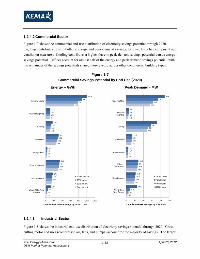
Figure 1-7 shows the commercial end-use distribution of electricity savings potential through 2020. Lighting contributes most to both the energy and peak-demand savings, followed by office equipment and ventilation measures. Cooling contributes a higher share to peak-demand savings potential versus energy-savings potential. Offices account for almost half of the energy and peak demand savings potential, with the remainder of the savings potentials shared more evenly across other commercial building types.
Figure 1-7 Commercial Savings Potential by End Use (2020)
Energy – GWh Peak Demand - MW
1,003
112
168
317
43
345
170
134
890
109
137
302
39
334
162
51
781
102
119
281
36
323
152
29
698
94
112
256
33
302
142
18
0 200 400 600 800 1,000 1,200
Indoor Lighting
Outdoor Lighting
Cooling
Ventilation
Refrigeration
Of f ice Equipment
Miscellaneous
Whole Bldg (New Constr)
Cumulative Annual Savings by 2020 - GWh
100% Incent75% Incent50% IncentBAU Incent
89.5
6.0
71.8
14.5
5.2
28.3
21.9
24.9
74.3
5.8
58.1
13.7
4.7
27.4
20.8
9.4
61.7
5.5
50.4
12.7
4.4
26.4
19.4
5.4
55.6
5.0
47.8
11.5
4.0
24.8
18.2
3.3
0 20 40 60 80 100
Indoor Lighting
Outdoor Lighting
Cooling
Ventilation
Refrigeration
Off ice Equipment
Miscellaneous
Whole Bldg (New Constr)
Cumulative Peak Savings by 2020 - MW
100% Incent75% Incent50% IncentBAU Incent
1.2.4.3 Industrial Sector
Figure 1-8 shows the industrial end-use distribution of electricity savings potential through 2020. Cross-cutting motor end uses (compressed air, fans, and pumps) account for the majority of savings. The largest
DSM Market Potential Assessment 1–12

Xcel Energy Minnesota April 20, 2012
industries in terms of savings potential are the food processing and petroleum refining industries, followed by chemicals, plastics, industrial machinery, and electronics.
Figure 1-8 Industrial Savings Potential by End Use (2020)
Energy – GWh Peak Demand - MW
208
269
179
128
45
75
18
11
72
195
208
166
110
40
72
16
11
71
183
176
155
98
36
67
14
10
68
170
150
141
86
32
59
12
9
66
0 100 200 300
Compressed Air
Fans
Pumping
Drives
Process Heating
Refrigeration
Other Process
Cooling
Lighting
Cumulative Annual Savings by 2020 - GWh
100% Incent75% Incent50% IncentBAU Incent
23.7
25.2
17.4
15.8
5.8
9.0
2.3
1.0
10.5
22.0
18.5
15.9
13.5
5.1
8.6
2.0
0.9
10.2
20.6
15.1
14.7
12.0
4.6
8.0
1.8
0.9
9.9
19.0
12.5
13.3
10.5
4.0
7.0
1.6
0.8
9.5
0 10 20 3
Compressed Air
Fans
Pumping
Drives
Process Heating
Refrigeration
Other Process
Cooling
Lighting
Cumulative Peak Savings by 2020 - MW0
100% Incent75% Incent50% IncentBAU Incent
1.2.5 Behavioral-Conservation Results
Residential behavioral-conservation programs have shown some promise in motivating customers to use less energy. However, factors such as persistence and the realized amount of energy savings have not been confirmed over a significant period of time or across a wide range of customers. Program designs include indirect feedback approaches, which feature periodic energy information reports, sometimes with comparative information to stimulate competitive behaviors, and direct feedback interventions, such use of in-home energy-use monitors. Both types theoretically result in behaviors that decrease energy usage. For this analysis, we focused on indirect feedback methods since these are experiencing wider adoption by utilities across the U.S. While there is probably overlap in the impacts of these two methods, this overlap is not well understood. Consequently, we present potential impacts from the indirect approach,
DSM Market Potential Assessment 1–13
Xcel Energy Minnesota April 20, 2012 DSM Market Potential Assessment
1–14
with the understanding that these impacts may serve as a proxy for savings from both types of behavior-motivation methods.
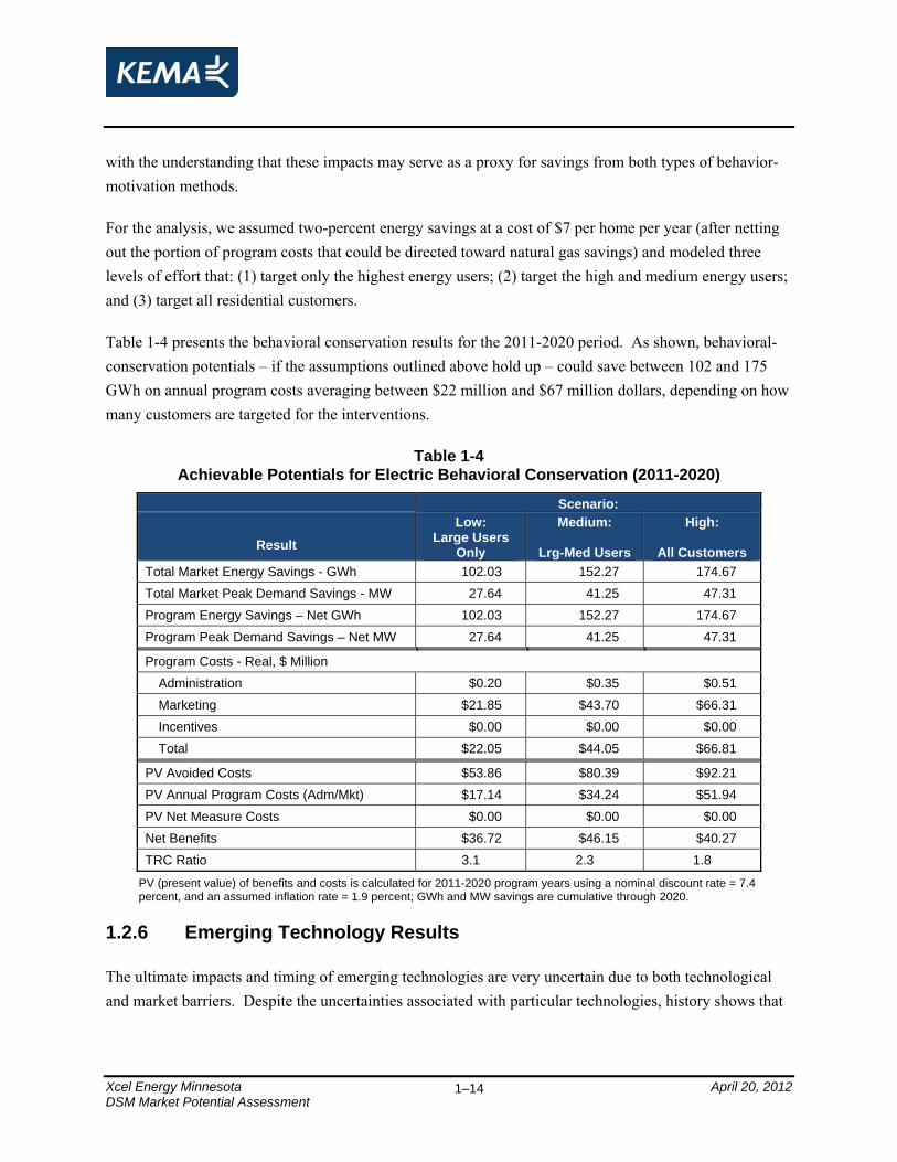
For the analysis, we assumed two-percent energy savings at a cost of $7 per home per year (after netting out the portion of program costs that could be directed toward natural gas savings) and modeled three levels of effort that: (1) target only the highest energy users; (2) target the high and medium energy users; and (3) target all residential customers.
Table 1-4 presents the behavioral conservation results for the 2011-2020 period. As shown, behavioral-conservation potentials – if the assumptions outlined above hold up – could save between 102 and 175 GWh on annual program costs averaging between $22 million and $67 million dollars, depending on how many customers are targeted for the interventions.
Table 1-4 Achievable Potentials for Electric Behavioral Conservation (2011-2020)
Scenario: Low: Medium: High:
Result Large Users Only Lrg-Med Users All Customers
Total Market Energy Savings - GWh 102.03 152.27 174.67 Total Market Peak Demand Savings - MW 27.64 41.25 47.31 Program Energy Savings – Net GWh 102.03 152.27 174.67 Program Peak Demand Savings – Net MW 27.64 41.25 47.31
Program Costs - Real, $ Million Administration $0.20 $0.35 $0.51 Marketing $21.85 $43.70 $66.31 Incentives $0.00 $0.00 $0.00 Total $22.05 $44.05 $66.81
PV Avoided Costs $53.86 $80.39 $92.21 PV Annual Program Costs (Adm/Mkt) $17.14 $34.24 $51.94 PV Net Measure Costs $0.00 $0.00 $0.00 Net Benefits $36.72 $46.15 $40.27 TRC Ratio 3.1 2.3 1.8
PV (present value) of benefits and costs is calculated for 2011-2020 program years using a nominal discount rate = 7.4 percent, and an assumed inflation rate = 1.9 percent; GWh and MW savings are cumulative through 2020.
1.2.6 Emerging Technology Results
The ultimate impacts and timing of emerging technologies are very uncertain due to both technological and market barriers. Despite the uncertainties associated with particular technologies, history shows that
Xcel Energy Minnesota April 20, 2012 DSM Market Potential Assessment
1–15
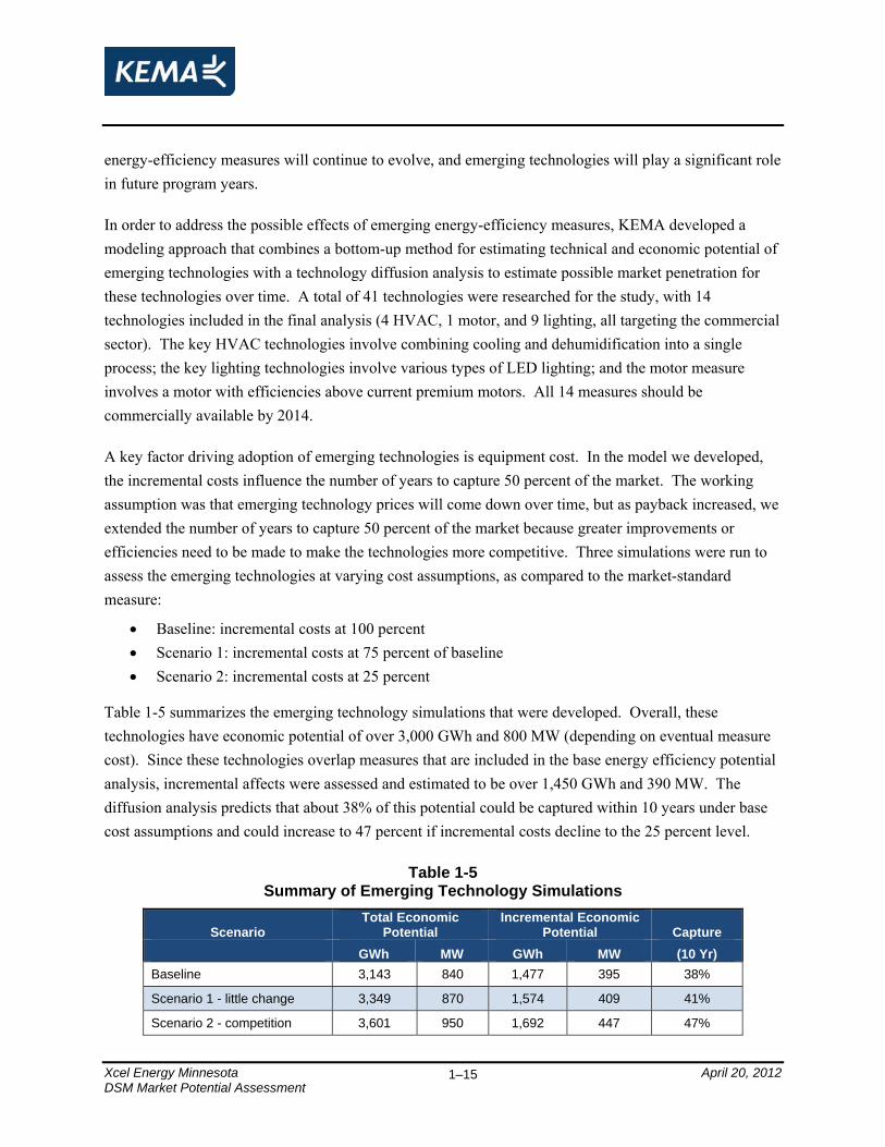
energy-efficiency measures will continue to evolve, and emerging technologies will play a significant role in future program years.
In order to address the possible effects of emerging energy-efficiency measures, KEMA developed a modeling approach that combines a bottom-up method for estimating technical and economic potential of emerging technologies with a technology diffusion analysis to estimate possible market penetration for these technologies over time. A total of 41 technologies were researched for the study, with 14 technologies included in the final analysis (4 HVAC, 1 motor, and 9 lighting, all targeting the commercial sector). The key HVAC technologies involve combining cooling and dehumidification into a single process; the key lighting technologies involve various types of LED lighting; and the motor measure involves a motor with efficiencies above current premium motors. All 14 measures should be commercially available by 2014.
A key factor driving adoption of emerging technologies is equipment cost. In the model we developed, the incremental costs influence the number of years to capture 50 percent of the market. The working assumption was that emerging technology prices will come down over time, but as payback increased, we extended the number of years to capture 50 percent of the market because greater improvements or efficiencies need to be made to make the technologies more competitive. Three simulations were run to assess the emerging technologies at varying cost assumptions, as compared to the market-standard measure:
• Baseline: incremental costs at 100 percent • Scenario 1: incremental costs at 75 percent of baseline • Scenario 2: incremental costs at 25 percent
Table 1-5 summarizes the emerging technology simulations that were developed. Overall, these technologies have economic potential of over 3,000 GWh and 800 MW (depending on eventual measure cost). Since these technologies overlap measures that are included in the base energy efficiency potential analysis, incremental affects were assessed and estimated to be over 1,450 GWh and 390 MW. The diffusion analysis predicts that about 38% of this potential could be captured within 10 years under base cost assumptions and could increase to 47 percent if incremental costs decline to the 25 percent level.
Table 1-5 Summary of Emerging Technology Simulations
Scenario Total Economic
Potential Incremental Economic
Potential Capture GWh MW GWh MW (10 Yr)
Baseline 3,143 840 1,477 395 38%
Scenario 1 - little change 3,349 870 1,574 409 41%
Scenario 2 - competition 3,601 950 1,692 447 47%

Xcel Energy Minnesota April 20, 2012
Figure 1-9 shows possible adoption paths for the emerging technologies under the baseline scenario and under Scenario 2, which reflects a 75 percent reduction in the incremental cost of the emerging technologies. (Note that the adoption path for Scenario 1, with a 25 percent cost reduction, was not very different than the baseline adoption path.) The figure shows that the HVAC measures are only affected somewhat by the drop in cost; these technologies already appear to be very cost effective with current equipment price assumptions. However, both the lighting and motor measures show substantially increased penetration if costs could drop significantly – either through market forces or from utility-provided incentives.
Figure 1-9 Emerging Technology Adoption Paths
Baseline Scenario 2 – 75% Cost Reduction
0
250
500
750
1,000
1,250
1,500
1,750
2,000
2,250
Cum
ulat
ive
Annu
al S
avin
gs -
GW
h
LightingHVACMotors
0
250
500
750
1,000
1,250
1,500
1,750
2,000
2,250
Cum
ulat
ive
Annu
al S
avin
gs -
GW
hLightingHVACMotors
1.2.7 Demand Response Results
Demand response potential estimates were developed using the NADR model as noted above. The model estimates impacts for four customer segments (residential and small, medium, and large nonresidential) and five DR program categories (direct load control, interruptible rates, dynamic pricing with enabling technologies, dynamic pricing without enabling technologies, and other DR programs such as demand bidding). Estimates are developed for four different scenarios:
• Business-as-usual (BAU): current programs and tariffs are held constant.
• Expanded BAU (EBAU): BAU program participation rates are increased to equal the 75th percentile of ranked participation rates of similar programs across the U.S.
• Achievable Participation (AP): further assumes advanced metering infrastructure (AMI) is universally deployed, and dynamic pricing is the opt-out default tariff.
DSM Market Potential Assessment 1–16

Xcel Energy Minnesota April 20, 2012 DSM Market Potential Assessment
1–17
• Full Participation (FP): similar to the AP scenario, except that dynamic pricing and the acceptance of enabling technology is mandatory. This scenario quantifies the maximum cost-effective DR potential, absent any regulatory and market barriers.
Table 1-6 summarizes the results of the DR potential analysis. Potential demand reductions by 2020 range from 941 MW in the BAU case to 1,209 MW in the Expanded BAU case to 1,444 MW in the Achievable Participation case to 1,552 in the Full Participation case. The primary sources of savings potential are interruptible rates and direct load control, with the pricing without enabling technologies mechanism also showing substantial savings for the Achievable and Full Participation scenarios. Pricing with enabling technologies was only cost effective for the medium C&I segment and does not contribute much to the DR potential. The residential segment accounts for between 32 percent and 44 percent of total DR potentials and the large C&I segment accounts for between 50 percent and 63 percent of total DR potentials, depending on the scenario.
Table 1-6 Summary of Demand Response Potential by 2020 - MW
DR Mechanism BAU Expanded
BAU Achievable
Participation* Full
Participation Pricing with Technology 0 0 13 37 Pricing without Technology 0 11 304 422 Automated/Direct Load Control 438 465 440 438 Interruptible/Curtailable Tariffs 503 643 643 643 Other DR Programs 0 90 44 12 Total 941 1,209 1,444 1,552
* Achievable Participation is the name given to a specific scenario in the FERC NADR study; these potentials are only achievable under the specific assumptions that define this scenario.
There are a number of barriers to achieving the DR potentials developed in this study, including:
• Limits to AMI installations required for critical peak pricing;
• Regulatory barriers that include reluctance to adopt dramatically different pricing structures and reluctance fund investments in AMI installations or in customer-side enabling technologies;
• Technology barriers such as the limitations on cost-effective enabling technologies; and,
• Customer barriers including: lack of awareness regarding DR, risk aversion to new technologies and pricing strategies, and perceived lack of ability to respond to DR events.
In addition, the analysis does not address the need for DR. It just shows the peak savings reductions possible if a number of different DR strategies are implemented. Identifying the optimal amount of DR for Xcel Energy’s Minnesota service territory, taking into account DR resources and existing generation and T&D capacity, is a planning exercise that is not part of this potential study.

Xcel Energy Minnesota April 20, 2012 DSM Market Potential Assessment
1–18
1.2.8 Uncertainty of Results
We want to caution the reader that there is inherent uncertainty in the results presented in this report because they are forecasts of what could happen in the future. Our estimates of technical and economic potential have the lowest degree of uncertainty. These are estimates that account for savings, costs, and current saturations of DSM measures but do not factor in human behavior.
The achievable program estimates do take into account behavior, as our modeling efforts try to predict program participation levels while factoring in measure awareness and economics, as well as barriers to measure uptake. Hence, the uncertainty in our achievable potential estimates is greater. This uncertainty is lowest for the BAU scenario as these results are most consistent with current program experience. Uncertainty is higher for the 75-percent and 100-percent incentive scenarios, as these scenarios are based on projections from limited historical experience. Uncertainty is greatest for the 100-percent incentive scenario because there is no “real world” program experience where all the incremental measure costs for all customer segments are paid for by the utility over an extended period of time. Typically, a utility may offer the equivalent of 100-percent incentives for limited measures and customer segments in order to overcome high barriers in specific markets and to gain a high level of program participation while limiting program costs.
Uncertainty around the results of the behavioral conservation analysis is rooted in the persistence of the measure. Early findings have shown that these types of measures can save in the neighborhood of two percent per year in the near term, but it is not clear whether ongoing customer feedback messages will be able to maintain the savings.
Emerging technologies have many inherent uncertainties, including: technology performance, corporate interest in supporting R&D efforts, equipment cost, and customer acceptance. Our efforts in this study attempted to minimize the first two sources on uncertainty by focusing on products that should be commercially viable in the next few years and that have sufficient producer support to ensure the likelihood of market deployment.
1.3 Conclusions As the results of this study indicate, there is a significant amount of DSM potential remaining in the Xcel Energy Minnesota service territory. The residential and commercial sectors provide the largest sources of identified potential savings. While savings potentials in the industrial sector are lower, this segment is more complex and less understood that the other sectors, and it is likely that our bottom-up analysis understates, to some degree, all the custom energy efficiency opportunities available in this sector.

Xcel Energy Minnesota April 20, 2012 DSM Market Potential Assessment
1–19
We note that Xcel Energy’s current programs, as modeled in the business-as-usual scenario, are expected to capture a significant amount of the available savings (about nine percent of base energy usage by 2020) at current program expenditure levels. These programs have developed over a number of years and appear to utilize program funding efficiently. While increased achievable savings are possible at increased levels of program effort, we caution that these increases could be expensive. The 75-percent incentive scenario shows a 16-percent increase in energy savings by 2020, but comes with a 181-percent increase in program costs. The 100-percent incentive scenario shows a 37-percent increase in energy savings by 2020, but comes with a 279-percent increase in program costs.
We also note that a dramatic increase in program activity over an extended period does not seem to be supported by the available energy efficiency resources. While the higher-incentive scenarios show large amounts of achievable potential over the first few years of the forecast horizon, an accelerated program approach is likely to lead to a substantial drop-off in program accomplishments in later years as many of the retrofit measure reach high saturation levels. This boom-bust phenomenon could be detrimental to long-term program sustainability and would likely reduce the ability of Xcel Energy’s program structure to accommodate emerging technologies and adapt to other market developments.
Additional conclusions, by topic area, are summarized below:
• Savings opportunities
o Residential sector – The potential is greatest for cooling, lighting, and furnace fan end use measures. Whole-building new constructions measures are also a large source of potential savings.
o Commercial sector – Lighting and HVAC measures continue to provide the largest sources of energy efficiency potential. Office equipment, including data center and server measures, also appears to be a substantial source of savings.
o Industrial sector – Cross-cutting motor-driven end uses (fans, pumps, and compressed air) offer the greatest potential in this sector, and are associated with measures that apply to a wide variety of industrial classifications.
• Behavioral conservation measures may also play a role in reducing energy consumption in Xcel Energy’s service territory. However, the persistence of behavior-oriented measures has not been tested over an extended period of time, so continued evaluation of behavioral conservation programs will be necessary to ensure that savings don’t dissipate over time.
• Emerging technologies will play an increasing role in the energy efficiency portfolio as traditional measures reach high market saturation levels. It may be necessary to initially offer fairly high incentives to promote some of the emerging technologies, especially the LED lighting technologies that have a high first cost compared to base technologies.

Xcel Energy Minnesota April 20, 2012 DSM Market Potential Assessment
1–20
• Demand response is already a significant part of Xcel Energy’s DSM portfolio, as shown by projected demand reductions of over 900 MW of by 2020 under business as usual. Additional savings of up to 300MW could possibly be acquired through current program augmentation, but further additions to savings that are tied to critical peak pricing would require investments in AMI, and those investments would need to be evaluated on many parameters in addition to the DR benefit.

Xcel Energy Minnesota April 20, 2012 DSM Market Potential Assessment
2–1
2. Introduction
2.1 Overview KEMA, Inc. (KEMA) was retained by Xcel Energy to conduct this demand-side management (DSM) market potential study. The study provides estimates of potential electricity and peak-demand savings from DSM measures in Xcel Energy’s Minnesota service territory.
The study was designed to:
1. Help determine how much electric technical, economic, achievable (market), and naturally occurring potential exists within Xcel Energy’s Minnesota service territory for cost-effective energy-efficiency and demand-response resources.
2. Be used to help inform the Company’s 2013 - 2015 triennial filings 3. Assist in establishing mechanisms by which the company can continuously evaluate opportunities
for cost-effective DSM, including but not limited to financial modeling. 4. Assess the impact of factors that may affect baseline assumption since the last potential study.
These factors may include changes in codes, standards and rates.
The scope of this study includes new and existing residential and nonresidential buildings, as well as industrial process savings. The study covers an 10-year period spanning 2011-2020. Given the near- to mid-term focus, the base potential analysis was restricted to DSM measures that are presently commercially available. In addition, a number of measures were evaluated as emerging technologies, for example LED lighting. While commercially available (or soon to be commercially available), these products are characterized by limited availability, low consumer awareness, uncertainty about average energy savings, and high current costs that have the potential to drop significantly with market adoption.
Data for the study come from a number of different sources, including primary data collected for this project, secondary sources that include internal Xcel Energy studies and data, as well as a variety of information from third parties. The primary data collection efforts for this study involved 300 residential on-site, 150 commercial on-site surveys, 50 industrial on-site surveys, 804 residential decision-maker telephone surveys, and 41 market actor interviews.
2.2 Study Approach This study involved identification and development of baseline end-use and measure data and development of estimates of future energy-efficiency impacts under varying levels of program effort. Residential, commercial, and industrial on-site surveys were utilized, in conjunction with telephone

Xcel Energy Minnesota April 20, 2012 DSM Market Potential Assessment
2–2
interviews of market actors and information from secondary sources, to aid in development of the baseline and measure data.
The baseline characterization allowed us to identify the types and approximate sizes of the various market segments that are the most likely sources of DSM potential in Xcel Energy’s Minnesota service territory. These characteristics then served as inputs to a modeling process that incorporated Xcel Energy energy-cost parameters and specific energy-efficiency measure characteristics (such as costs, savings, and existing penetration estimates) to provide more detailed potential estimates.
To aid in the analysis, we utilized the KEMA DSM ASSYST™ model. This model provides a thorough, clear, and transparent documentation database, as well as an extremely efficient data processing system for estimating technical, economic, and achievable potential. We estimated technical, economic, and achievable program potential for the residential, commercial, and industrial sectors, with a focus on energy-efficiency impacts over the next 10 years.
To estimate demand response (DR) impacts, we reviewed impacts from the Federal Energy Regulatory Commission’s 2009 National Assessment of Demand Response Potential2 for the State of Minnesota and customized the results to the Xcel Energy Minnesota service territory, utilizing information on Xcel Energy’s peak demand relative to the Minnesota peak demand and information on current programs being run by Xcel Energy.
2.3 Layout of the Report Section 3 discusses the methodology and concepts used to develop the technical, economic, and achievable potential estimates. Section 4 provides baseline results developed for the study. Section 5 discusses the results of the electric energy-efficiency potential analysis by sector and over time. Section 6 presents demand-response potential results.
The report contains the following appendices:
• Appendix A: Detailed Methodology and Model Description – Further detail on what was discussed in Section 2.
• Appendix B: Measure Descriptions – Describes the measures included in the study.
• Appendix C: Economic Inputs – Provides avoided cost, electric rate, discount rate, and inflation rate assumptions used for the study.
2 A National Assessment of Demand Response Potential, Staff Report, Federal Energy Regulatory Commission, prepared by The Brattle Group, Freeman, Sullivan & Co., and Global Energy Partners, LLC, June 2009

Xcel Energy Minnesota April 20, 2012 DSM Market Potential Assessment
2–3
• Appendix D: Building and TOU Factor Inputs – Shows the base household counts, square footage estimates for commercial building types, and base energy use by industrial segment. This appendix also includes time-of-use factors by sector and end-use.
• Appendix E: Measure Inputs – Lists the electric measures included in the analysis with the costs, estimated savings, applicability, and estimated current saturation factors.
• Appendix F: Non-Additive Measure Level Results – Shows energy-efficiency potential for each measure independent of any other measure.
• Appendix G: Supply-Curve Data – Shows the data behind the energy supply curves provided in Section 5 of the report.
• Appendix H: Achievable Program Potential – Provides the forecasts for the achievable potential scenarios.
• Appendix I: Residential On-Site Surveys – Summarizes the on-site survey results.
• Appendix J: Commercial On-Site Surveys – Summarizes the on-site survey results.
• Appendix K: Industrial On-Site Surveys – Summarizes the on-site survey results.
• Appendix L: Residential Awareness Research Report – Provides results of the telephone surveys.
• Appendix M: Market Actor Research Report – Provides results of interviews with market actors.
• Appendix N: Benchmarking of Demand Response Potentials Report – Summarizes inputs and outputs of the Demand Response analysis.

Xcel Energy Minnesota April 20, 2012 DSM Market Potential Assessment
3–1
3. Methods and Scenarios
This section provides a brief overview of the concepts, methods, and scenarios used to conduct this study. Additional methodological details are provided in Appendix A.
3.1 Characterizing the Energy-Efficiency Resource Energy efficiency has been characterized for some time now as an alternative to energy supply options, such as conventional power plants that produce electricity from fossil or nuclear fuels. In the early 1980s, researchers developed and popularized the use of a conservation supply-curve paradigm to characterize the potential costs and benefits of energy conservation and efficiency. Under this framework, technologies or practices that reduced energy use through efficiency were characterized as “liberating ‘supply’ for other energy demands” and could therefore be thought of as a resource and plotted on an energy supply curve. The energy-efficiency resource paradigm argued simply that the more energy efficiency or “nega-watts” produced, the fewer new plants would be needed to meet end-users’ power demands.
3.1.1 Defining Energy-Efficiency Potential
Energy-efficiency potential studies were popular throughout the utility industry from the late 1980s through the mid-1990s. This period coincided with the advent of what was called least-cost or integrated resource planning (IRP). Energy-efficiency potential studies became one of the primary means of characterizing the resource availability and value of energy efficiency within the overall resource planning process.
Like any resource, there are a number of ways in which the energy-efficiency resource can be estimated and characterized. Definitions of energy-efficiency potential are similar to definitions of potential developed for finite fossil-fuel resources, like coal, oil, and natural gas. For example, fossil-fuel resources are typically characterized along two primary dimensions: the degree of geological certainty with which resources may be found and the likelihood that extraction of the resource will be economic. This relationship is shown conceptually in Figure 3-1.
Somewhat analogously, this energy-efficiency potential study defines several different types of energy-efficiency potential, namely, technical, economic, achievable program, and naturally occurring. These potentials are shown conceptually in Figure 3-2 and described below.
• Technical potential is defined in this study as the complete penetration of all measures analyzed in applications where they were deemed technically feasible from an engineering perspective.

Xcel Energy Minnesota April 20, 2012
Figure 3-1 Conceptual Framework for Estimates of Fossil Fuel Resources
Decreasing Economic Feasibility
Dec
reas
ing
Cer
tain
ty o
f Exi
sten
cePossible
and Economically Feasible
Possiblebut not
Economically Feasible
Knownbut not
Economically Feasible
Knownand
Economically Feasible
• Economic potential refers to the technical potential of those energy conservation measures that are cost effective when compared to supply-side alternatives.
• Achievable program potential refers to the amount of savings that would occur in response to specific program funding and measure incentive levels. Savings associated with program potential are savings that are projected beyond those that would occur naturally in the absence of any market intervention.
• Naturally occurring potential refers to the amount of savings estimated to occur as a result of normal market forces; that is, in the absence of any utility or governmental intervention.
DSM Market Potential Assessment 3–2

Xcel Energy Minnesota April 20, 2012
Figure 3-2 Conceptual Relationship among Energy-Efficiency Potential Definitions
Achievable Program
Technical
Economic
Naturally Occurring
Achievable Program
Technical
Economic
Naturally Occurring
3.2 Summary of Analytical Steps Used in this Study The crux of this study involves carrying out a number of basic analytical steps to produce estimates of the energy-efficiency potentials introduced above. The basic analytical steps for this study are shown in relation to one another in Figure 3-3. The bulk of the analytical process for this study was carried out in a model developed by KEMA for conducting energy-efficiency potential studies. Details on the steps employed and analyses conducted are described in Appendix A. The model used, DSM ASSYST™, is a Microsoft Excel®-based model that integrates technology-specific engineering and customer behavior data with utility market saturation data, load shapes, rate projections, and marginal costs into an easily updated data management system.
DSM Market Potential Assessment 3–3

Xcel Energy Minnesota April 20, 2012
Figure 3-3 Conceptual Overview of Study Process
Building DataEnd Use Saturation
End Use ConsumptionLoadshapes
Building ft2, # Homes
Building DataEnd Use Saturation
End Use ConsumptionLoadshapes
Building ft2, # Homes
Measure DataCosts
SavingsCurrent Saturation
Measure DataCosts
SavingsCurrent Saturation
Program Data and
Adoption Inputs
Economic Potential
Economic Potential
TechnicalPotentialTechnicalPotential
NaturallyOccurring Efficiency
NaturallyOccurring Efficiency
Model InputsModel Inputs
Sce n ar io s
Economic DataAvoided Costs
RatesDiscount/Inflation Rate
Economic DataAvoided Costs
RatesDiscount/Inflation Rate
Achievable Program Potential
The key steps implemented in this study are:
Step 1: Develop Initial Input Data
• Develop a list of energy-efficiency measure opportunities to include in scope. In this step, an initial draft measure list was developed and circulated internally within Xcel Energy and to an external advisory group. The final measure list was developed after incorporating comments.
• Gather and develop technical data (costs and savings) on efficient measure opportunities. Data on measures were gathered from a variety of sources. Measure descriptions are provided in Appendix B, and detail on measure inputs is provided in Appendix E.
• Gather, analyze, and develop information on building characteristics, including total square footage or total number of households, energy consumption and intensity by end use, end-use consumption load patterns by time of day and year (i.e., load shapes), market shares of key electric consuming equipment, and market shares of energy-efficiency technologies and practices. Section 4 of this report describes the baseline data developed for this study.
To aid in development of baseline data for the project, several primary data collection efforts were undertaken:
DSM Market Potential Assessment 3–4
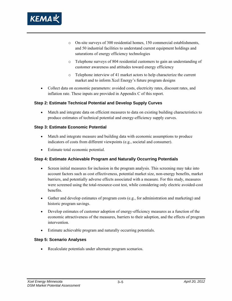
Xcel Energy Minnesota April 20, 2012 DSM Market Potential Assessment
3–5
o On-site surveys of 300 residential homes, 150 commercial establishments, and 50 industrial facilities to understand current equipment holdings and saturations of energy efficiency technologies
o Telephone surveys of 804 residential customers to gain an understanding of customer awareness and attitudes toward energy efficiency
o Telephone interview of 41 market actors to help characterize the current market and to inform Xcel Energy’s future program designs
• Collect data on economic parameters: avoided costs, electricity rates, discount rates, and inflation rate. These inputs are provided in Appendix C of this report.
Step 2: Estimate Technical Potential and Develop Supply Curves
• Match and integrate data on efficient measures to data on existing building characteristics to produce estimates of technical potential and energy-efficiency supply curves.
Step 3: Estimate Economic Potential
• Match and integrate measure and building data with economic assumptions to produce indicators of costs from different viewpoints (e.g., societal and consumer).
• Estimate total economic potential.
Step 4: Estimate Achievable Program and Naturally Occurring Potentials
• Screen initial measures for inclusion in the program analysis. This screening may take into account factors such as cost effectiveness, potential market size, non-energy benefits, market barriers, and potentially adverse effects associated with a measure. For this study, measures were screened using the total-resource-cost test, while considering only electric avoided-cost benefits.
• Gather and develop estimates of program costs (e.g., for administration and marketing) and historic program savings.
• Develop estimates of customer adoption of energy-efficiency measures as a function of the economic attractiveness of the measures, barriers to their adoption, and the effects of program intervention.
• Estimate achievable program and naturally occurring potentials.
Step 5: Scenario Analyses
• Recalculate potentials under alternate program scenarios.

Xcel Energy Minnesota April 20, 2012 DSM Market Potential Assessment
3–6
3.3 Scenario Analysis Scenario analysis is a tool commonly used to structure the uncertainty and examine the robustness of projected outcomes to changes in key underlying assumptions. This section describes the alternative scenarios under which demand-side management (DSM) potential was estimated in this study. We developed these scenarios of DSM potential for two key reasons:
1. Our estimates of potential depend on future adoptions of energy-efficiency measures that are a function of data inputs and assumptions, which are themselves forecasts. For example, our projections depend on estimates of measure availability, measure cost, measure savings, measure saturation levels, retail rates, and avoided costs. Each of the inputs to our analysis is subject to some degree of uncertainty.
2. The ultimate achievable energy-efficiency potential depends, by definition, on policy choices, including the level of resources and strategies used to increase measure adoption.
The cost components of program funding that vary under each scenario include:
Marketing and Education Expenditures
• Customers must be aware of efficiency measures and their associated benefits in order to adopt those measures. In our analysis, program marketing expenditures are converted to increases in awareness. Thus, under higher levels of marketing expenditures, higher levels of awareness are achieved.
Incentives and Direct Implementation Expenditures
• The higher the percentage of measure costs paid by the program, the higher the participants’ benefit-cost ratios and, consequently, the number of measure adoptions.
Administration Expenditures
• Purely administrative costs, though necessary and important to the program process, do not directly lead to adoptions; however, they have been included in program funding because they are an input to program benefit-cost tests.
For the study, the primary analysis focused a base case consisting of commercially available, established efficiency technologies. In addition to this base analysis, we analyzed:
• Emerging technologies • Behavioral-conservation measures • Demand response

Xcel Energy Minnesota April 20, 2012 DSM Market Potential Assessment
3–7
For each analysis, four program-funding scenarios were considered: a business-as-usual (BAU) funding scenario, a 50-percent incentive scenario, a 75-percent incentive scenario, and a 100-percent incentive scenario. These scenarios are discussed below.
In all scenarios, a number of measures were modeled without financial incentives. These include office equipment power-management enabling, industrial operations and maintenance (O&M) measures, and Energy Star office equipment and consumer electronics for the residential sector. Because these measures are very cost effective, it was deemed that provision of an incentive would primarily benefit free riders.
Note for the low-income segment, all scenarios reflect 100 percent incentives (as a percent of incremental measure cost). Program effort was adjusted across scenarios such that low-income program potentials roughly track other residential program potentials.
3.3.1 Business as Usual (BAU) Incentive Scenario
In this scenario we modeled existing Xcel Energy programs and incentive levels. This scenario was used to calibrate the DSM Assyst model to equate current incentive and other program effort expenditures to expect program savings. Incentives (as a percent of incremental measure costs) varied by measure in this scenario. Average incentives, by sector, utilized for this scenario were: 59 percent for the residential sector, 30 percent for the commercial sector, and 28 percent for the industrial sector.
3.3.2 Fifty-percent Incentive Scenario
In the 50-percent incentive scenario, base incentive levels are set to 50 percent of incremental measure costs. Marketing/customer education and administration budgets were increased from current Xcel Energy budgets. For the behavioral conservation program, which isn’t tied to incentives, we extended the program to cover only the largest residential energy users. Program administration budgets are set at modest amounts, roughly corresponding to minimum program support levels.
3.3.3 Seventy-five-percent Incentive Scenario
In this scenario, incentives were increased to cover 75 percent of incremental measure costs, except for the low-income giveaway items and measures that had constrained incentives as discussed above. For the behavioral conservation program, we extended coverage to both the large and medium sized residential energy users. Program marketing and administration budgets were also increased for this scenario.

Xcel Energy Minnesota April 20, 2012 DSM Market Potential Assessment
3–8
3.3.4 One-hundred-percent Incentive Scenario
In this scenario, incentives were increased to cover 100 percent of incremental measure costs, with the exception of constrained measures. The behavioral conservation program was extended to cover all residential customers. Program marketing and administration budgets were increased again for this scenario.
3.3.5 Summary of Scenarios
Table 3-1 shows average spending on electricity programs for each of the scenarios for the 2011-2020 forecast period for the base analysis, which does not include emerging technologies, behavioral-conservation measures, or demand response.

Xcel Energy Minnesota April 20, 2012 DSM Market Potential Assessment
3–9
Table 3-1 Scenario Average Spending during 2011-2020 Forecast Period ($1000s)
Electric Programs
% Incremental Funding Market Cost Components Measure Cost
Level Segment Admin Marketing Incentives Total Paid* BAU Residential Existing $7,701 $4,499 $9,618 $21,818 58% Incentives Residential New Construction $637 $949 $1,064 $2,650 58% Residential Low Income $908 $726 $6,530 $8,164 100% Commercial Existing $5,446 $3,218 $11,324 $19,988 30% Commercial New Construction $28 $74 $296 $398 25% Industrial $2,028 $2,084 $4,195 $8,308 28% Total $16,750 $11,549 $33,027 $61,326 50% Residential Existing $7,521 $4,323 $11,487 $23,330 50% Incentives Residential New Construction $564 $902 $791 $2,257 50% Residential Low Income $930 $798 $6,653 $8,382 100% Commercial Existing $5,924 $3,779 $16,384 $26,088 50% Commercial New Construction $42 $88 $947 $1,078 50% Industrial $2,389 $2,501 $9,065 $13,954 50% Total $17,371 $12,391 $45,327 $75,089 75% Residential Existing $8,620 $4,755 $23,881 $37,256 75% Incentives Residential New Construction $847 $992 $1,958 $3,797 75% Residential Low Income $954 $878 $6,788 $8,620 100% Commercial Existing $6,638 $4,157 $27,539 $38,334 75% Commercial New Construction $68 $97 $2,483 $2,648 75% Industrial $2,890 $2,751 $14,672 $20,313 75% Total $20,017 $13,630 $77,322 $110,969 100% Residential Existing $10,215 $5,230 $48,296 $63,742 100% Incentives Residential New Construction $1,385 $1,091 $4,680 $7,156 100% Residential Low Income $981 $966 $6,935 $8,881 100% Commercial Existing $7,768 $4,573 $40,791 $53,132 100% Commercial New Construction $166 $107 $8,994 $9,267 100% Industrial $3,875 $3,026 $21,952 $28,853 100% Total $24,390 $14,993 $131,648 $171,032
3.3.6 Avoided-Cost Scenarios
The avoided-cost assumptions used in the study are based on the marginal energy cost forecast that Xcel Energy provided in October 2011. This base forecast resulted in a 5 percent reduction from the assumptions filed in 2010-2012 Minnesota DSM Triennial Plan. In order to test the sensitivity of the potential analysis to varying avoided costs, we also developed estimates of energy efficiency potential using lower and higher cost assumptions.

Xcel Energy Minnesota April 20, 2012 DSM Market Potential Assessment
3–10
The electric avoided costs were developed by time-of-use (TOU) period. These periods are shown in Table 3-2. Figure 3-4 shows the base electric avoided-cost forecast by TOU period. Figure 3-5 provides a comparison of the base, low, and high forecasts using load-weighted averages of the TOU forecasts. Overall, the high-cost forecast is about 57 percent higher than the base forecast, and the low-cost forecast is about 5 percent lower than the base forecast (before. Note that all forecasts include adders for environmental externalities (CO2 and SOx) and adders for non-energy benefits. In addition to energy avoided costs, capacity avoided costs are included in the analysis, starting at $121 per kW and increasing by about 2 percent per year.
Table 3-2 Electric Time-of-Use Period Definitions
TOU Period Weekday Hours Weekend Hours
Summer Off-Peak 0:01-6:00 0:01-8:00
Summer Mid-Peak 6:01-7:00, 23:01-24:00 8:01-9:00, 22:01-24:00
Summer On-Peak 7:01-12:00, 17:01-23:00 9:01-22:00
Summer Super-Peak 12:01-17:00
Winter Off-Peak 0:01-6:00, 23:01-24:00 0:01-9:00, 23:01-24:00
Winter On-Peak 6:01-23:00 9:01-23:00
Summer June-September
Winter October-May * Time-of-use periods were determined by analysis of hourly marginal costs to identify periods that have similar prices. These periods are independent of any billing TOU rates.

Xcel Energy Minnesota April 20, 2012
Figure 3-4 Electric Avoided-Cost Forecast - Base
$0.00
$0.01
$0.02
$0.03
$0.04
$0.05
$0.06
$0.07
$0.08
$0.09
$0.10
$ pe
r kWh
2011 2012 2013 2014 2015 2016 2017 2018 2019 2020
Summer Super PeakSummer On PeakSummer Mid PeakSummer Off PeakWinter On PeakWinter Off Peak
Figure 3-5 Electric Avoided-Cost Forecast Comparison
$0.000
$0.010
$0.020
$0.030
$0.040
$0.050
$0.060
$0.070
$0.080
$0.090
$0.100
2011 2012 2013 2014 2015 2016 2017 2018 2019 2020
$ pe
r kWh
High‐Average
Base‐Average
Low‐Average
DSM Market Potential Assessment 3–11

Xcel Energy Minnesota April 20, 2012 DSM Market Potential Assessment
4–1
4. Baseline Results
4.1 Overview Estimating the potential for energy-efficiency improvements requires a comparison of the energy impacts of standard-efficiency technologies with those of alternative high-efficiency equipment. This, in turn, dictates a relatively detailed understanding of the energy characteristics of the marketplace. Baseline data that were required for each studied market segment includes:
• Total count of energy-consuming units (floor space of commercial buildings, number of residential dwellings, and the base kWh consumption of industrial facilities)
• Annual energy consumption for each end use studied (both in terms of total consumption in GWh and normalized for intensity on a per-unit basis (e.g., kWh/ft2)
• End-use load shapes (that describe the amount of energy used or power demand over certain times of the day and days of the year)
• The saturation of electric end uses (e.g., the fraction of total commercial floor space with electric air conditioning)
• The market share of each base equipment type for example, the fraction of total commercial floor space served by 4-foot fluorescent lighting fixtures)
• Market share for each energy-efficiency measure in scope (for example, the fraction of total commercial floor space already served by CFLs).
Data for the baseline analysis comes from a number of sources, including Xcel Energy billing data extracts, Xcel Energy internal studies and analyses, U.S. Department of Energy studies, on-site surveys, and other secondary sources. Baseline data sources vary by sector and are described further below.
Figure 4-1 shows the overall breakdown of electricity use and peak demand by sector for the Xcel Energy Minnesota service territory. The commercial sector accounts for the largest share of energy usage, followed by the residential, industrial, and TCU (transportation, communications, and utilities) sectors. The chart breaks out “opt-out” customers. These are commercial and industrial customers that as of October 1, 2011 had opted out of Minnesota’s Resource Adjustment Rider and are therefore ineligible for Xcel Energy’s efficiency and demand response programs (see section 1.1 for further discussion). While we identify them here in the context of Xcel’s total customer base, they are excluded from the remainder of the analysis since as opt-outs they cannot contribute to program potential.

Xcel Energy Minnesota April 20, 2012
Figure 4-1 Electricity Usage Breakdown – Xcel Energy Minnesota Service Territory
Residential28.9%
Commercial42.7%
Industrial (including
WWT)21.5%
Opt-Outs0.9%Agriculture
0.4%
Mining0.2%
Costruction1.0%
TCU (except WWT)2.5%
Unclassif ied1.9%
Total Electric Use 28,111 GWh
Source: Xcel Energy Billing Records
Table 4-1 shows the results of the nonresidential billing analysis. Note that at the bottom of the table we show an unclassified category. These categories account for only 2.7 percent of nonresidential electricity use. Detailed results of the billing analysis by sector are reported in the sector-specific sections below.
DSM Market Potential Assessment 4–2

Xcel Energy Minnesota April 20, 2012 DSM Market Potential Assessment
4–3
Table 4-1 Results of Nonresidential Billing Analysis
SECTOR BUSINESS TYPE # of Sites kWh % of kWh
AG Agriculture 2,278 120,602,970 0.6% COM College 733 299,093,618 1.4% COM Com misc 8,543 1,181,007,404 5.6% COM Grocery 1,859 629,625,523 3.0% COM Health 701 476,726,003 2.3% COM Lodging 898 345,952,865 1.6% COM Office-L 271 2,647,088,675 12.6% COM Office-S 47,250 2,995,139,537 14.2% COM Restaurant 4,715 652,125,308 3.1% COM Retail-L 91 447,797,056 2.1% COM Retail-S 14,273 1,235,200,928 5.9% COM School 1,377 559,105,741 2.7% COM Warehouse 6,642 1,208,700,827 5.7% CST Construction 5,937 294,274,373 1.4% IND Chemicals 305 584,987,128 2.8% IND Electronics 481 438,973,482 2.1% IND Fabricated metals 648 295,426,049 1.4% IND Food 485 981,997,945 4.7% IND Ind machinery 1,198 507,483,821 2.4% IND Ind misc 948 420,602,887 2.0% IND Paper 175 389,462,178 1.8% IND Petroleum 55 1,073,932,634 5.1% IND Plastics 378 439,621,890 2.1% IND Primary metals 184 548,282,354 2.6% IND Printing 940 375,279,206 1.8% IND Stone-clay-glass 260 224,673,531 1.1% IND Textiles 223 26,557,686 0.1% IND Transp equip 216 131,672,489 0.6% IND Wood 442 167,015,964 0.8% MIN Mining 127 48,306,675 0.2% TCU Tcu 6,010 715,056,269 3.4% TCU Water-WWT 120 82,195,101 0.4% UNC Unclassified 12,610 540,897,823 2.6%
Total NonRes 121,373 21,084,865,940
Source: Xcel Energy Minnesota billing analysis
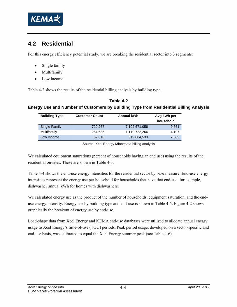
Xcel Energy Minnesota April 20, 2012 DSM Market Potential Assessment
4–4
4.2 Residential For this energy efficiency potential study, we are breaking the residential sector into 3 segments:
• Single family • Multifamily • Low income
Table 4-2 shows the results of the residential billing analysis by building type.
Table 4-2 Energy Use and Number of Customers by Building Type from Residential Billing Analysis
Building Type Customer Count Annual kWh Avg kWh per household
Single Family 720,267 7,102,671,058 9,861 Multifamily 264,635 1,110,722,266 4,197 Low Income 67,610 519,884,533 7,689
Source: Xcel Energy Minnesota billing analysis
We calculated equipment saturations (percent of households having an end use) using the results of the residential on-sites. These are shown in Table 4-3.
Table 4-4 shows the end-use energy intensities for the residential sector by base measure. End-use energy intensities represent the energy use per household for households that have that end-use, for example, dishwasher annual kWh for homes with dishwashers.
We calculated energy use as the product of the number of households, equipment saturation, and the end-use energy intensity. Energy use by building type and end-use is shown in Table 4-5. Figure 4-2 shows graphically the breakout of energy use by end-use.
Load-shape data from Xcel Energy and KEMA end-use databases were utilized to allocate annual energy usage to Xcel Energy’s time-of-use (TOU) periods. Peak period usage, developed on a sector-specific and end-use basis, was calibrated to equal the Xcel Energy summer peak (see Table 4-6).

Xcel Energy Minnesota April 20, 2012 DSM Market Potential Assessment
4–5
Table 4-3 Residential End-Use Saturations by Base Measure
Single Family Multifamily Low Income
Base Split-System Air Conditioner (11 SEER) 74% 47% 38% Base Early Replacement Split-System Air Conditioner (11 SEER) 13% 8% 7% Base Room Air Conditioner - EER 9.7 14% 30% 45% Base Early Replacement Room Air Conditioner- EER 9.0 2% 5% 8% Base Dehumidifier- New Federal Standard 8% 6% 10% Base Furnace Fans 48% 17% 38% Base Resistance Space Heating (Primary) 9% 9% 12% Base High-Efficiency Incandescent Lighting,<1.15 hrs/day 100% 100% 100% Base High-Efficiency Incandescent Lighting,1.15-2.15 hrs/day 100% 100% 100% Base High-Efficiency Incandescent Lighting,2.15-5 hrs/day 100% 100% 100% Base High-Efficiency Incandescent Lighting,>5 hrs/day 100% 100% 100% Base Lighting 15 Watt CFL, <1.15 hrs/day 100% 100% 100% Base Lighting 15 Watt CFL, 1.15-2.15 hrs/day 100% 100% 100% Base Lighting 15 Watt CFL, 2.15-5 hrs/day 100% 100% 100% Base Lighting 15 Watt CFL, >5 hrs/day 100% 100% 100% Base Fluorescent Fixture 1.8 hrs/day 100% 100% 100% Base Refrigerator 85% 85% 85% Base Early Replacement Refrigerator 15% 15% 15% Base Second Refrigerator 18% 33% 27% Base Freezer 33% 38% 31% Base Early Replacement Freezer 6% 7% 6% Base 40 gal. Water Heating (EF=0.88) 7% 7% 3% Base Early Replacement Water Heating to Heat Pump Water Heater 1% 1% 0% Base Clothes Washer (MEF=1.26) 83% 87% 83% Base Clothes Dryer (EF=3.01) 45% 43% 40% Base Dishwasher (EF=0.65) 67% 80% 81% Base Single Speed Pool Pump (RET) 0% 0% 0% Base Two Speed Pool Pump (1.5 hp) (ROB) 0% 0% 0% Base Plasma TV 10% 13% 9% Base LCD TV 68% 56% 64% Base CRT TV 79% 62% 78% Base Set-Top Box 73% 67% 71% Base DVD Player 84% 80% 72% Base Desktop PC 68% 62% 51% Base Laptop PC 72% 66% 35% Base Cooking 61% 65% 53% Base Miscellaneous 100% 100% 100% Base House Practices 100% 100% 100%
Source: Residential on-site survey data

Xcel Energy Minnesota April 20, 2012 DSM Market Potential Assessment
4–6
Table 4-4 Residential End-Use Energy Intensities (kWh/household with end-use)
Single Family Multifamily Low Income
Base Split-System Air Conditioner (11 SEER) 1,789 322 1,321 Base Early Replacement Split-System Air Conditioner (11 SEER) 2,236 403 1,652 Base Room Air Conditioner - EER 9.7 773 315 736 Base Early Replacement Room Air Conditioner- EER 9.0 827 337 788 Base Dehumidifier- New Federal Standard 1,064 351 851 Base Furnace Fans 1,105 332 978 Base Resistance Space Heating (Primary) 5,658 1,700 5,007 Base High-Efficiency Incandescent Lighting,<1.15 hrs/day 133 66 64 Base High-Efficiency Incandescent Lighting,1.15-2.15 hrs/day 575 284 277 Base High-Efficiency Incandescent Lighting,2.15-5 hrs/day 249 123 120 Base High-Efficiency Incandescent Lighting,>5 hrs/day 377 186 182 Base Lighting 15 Watt CFL, <1.15 hrs/day 6 3 4 Base Lighting 15 Watt CFL, 1.15-2.15 hrs/day 51 22 29 Base Lighting 15 Watt CFL, 2.15-5 hrs/day 45 19 25 Base Lighting 15 Watt CFL, >5 hrs/day 67 29 38 Base Fluorescent Fixture 1.8 hrs/day 242 62 84 Base Refrigerator 790 575 773 Base Early Replacement Refrigerator 790 575 773 Base Second Refrigerator 1,071 842 1,089 Base Freezer 549 549 549 Base Early Replacement Freezer 549 549 549 Base 40 gal. Water Heating (EF=0.88) 4,516 3,447 4,516 Base Early Replacement Water Heating to Heat Pump Water Heater 4,516 3,447 4,516 Base Clothes Washer (MEF=1.26) 81 81 81 Base Clothes Dryer (EF=3.01) 969 583 776 Base Dishwasher (EF=0.65) 162 162 162 Base Single Speed Pool Pump (RET) 822 822 822 Base Two Speed Pool Pump (1.5 hp) (ROB) 419 419 419 Base Plasma TV 235 235 268 Base LCD TV 158 142 165 Base CRT TV 186 123 208 Base Set-Top Box 234 197 233 Base DVD Player 33 26 34 Base Desktop PC 729.5 571.8 684.6 Base Laptop PC 191.9 168.5 170.2 Base Cooking 316 316 316 Base Miscellaneous 1,803 34 1,800 Base House Practices 9,861 4,197 7,689
Source: Various sources, calibrated to overall Xcel Energy consumption per household

Xcel Energy Minnesota April 20, 2012 DSM Market Potential Assessment
4–7
Table 4-5 Residential Energy Use by Building Type and End-Use
Single Family Multifamily Low Income Total
Base Split-System Air Conditioner (11 SEER) 949,555 39,908 34,176 1,023,639 Base Early Repl Split-System Air Conditioner (11 SEER) 209,461 8,803 7,539 225,803 Base Room Air Conditioner - EER 9.7 76,694 24,941 22,240 123,875 Base Early Replacement Room Air Conditioner- EER 9.0 14,482 4,710 4,199 23,391 Base Dehumidifier- New Federal Standard 63,148 5,984 5,795 74,928 Base Furnace Fans 386,034 15,090 25,368 426,492 Base Resistance Space Heating (Primary) 355,364 39,050 41,638 436,052 Base High-Efficiency Incandescent Lighting,<1.15 hrs/day 96,014 17,397 4,339 117,750 Base High-Efficiency Incandescent Lighting,1.15-2.15 hrs/day 414,177 75,045 18,718 507,940 Base High-Efficiency Incandescent Lighting,2.15-5 hrs/day 179,513 32,526 8,113 220,152 Base High-Efficiency Incandescent Lighting,>5 hrs/day 271,532 49,199 12,271 333,003 Base Lighting 15 Watt CFL, <1.15 hrs/day 4,545 723 240 5,508 Base Lighting 15 Watt CFL, 1.15-2.15 hrs/day 36,868 5,863 1,951 44,682 Base Lighting 15 Watt CFL, 2.15-5 hrs/day 32,067 5,100 1,697 38,864 Base Lighting 15 Watt CFL, >5 hrs/day 48,505 7,714 2,567 58,786 Base Fluorescent Fixture 1.8 hrs/day 174,235 16,496 5,685 196,417 Base Refrigerator 483,874 129,295 44,395 657,564 Base Early Replacement Refrigerator 85,389 22,817 7,834 116,041 Base Second Refrigerator 135,815 73,268 19,587 228,670 Base Freezer 130,507 55,748 11,635 197,889 Base Early Replacement Freezer 23,031 9,838 2,053 34,922 Base 40 gal. Water Heating (EF=0.88) 223,074 66,752 9,178 299,004 Base Early Repl Water Heating to Heat Pump Water Heater 24,786 7,417 1,020 33,223 Base Clothes Washer (MEF=1.26) 48,465 18,496 4,549 71,510 Base Clothes Dryer (EF=3.01) 314,980 67,024 21,128 403,132 Base Dishwasher (EF=0.65) 78,178 34,262 8,827 121,267 Base Single Speed Pool Pump (RET) 2,368 870 - 3,238 Base Two Speed Pool Pump (1.5 hp) (ROB) 1,208 444 - 1,651 Base Plasma TV 16,934 7,770 1,660 26,363 Base LCD TV 77,158 20,961 7,114 105,233 Base CRT TV 106,235 20,018 10,944 137,197 Base Set-Top Box 123,215 34,770 11,106 169,091 Base DVD Player 20,083 5,581 1,645 27,309 Base Desktop PC 359,468 93,777 23,533 476,778 Base Laptop PC 98,900 29,530 4,077 132,507 Base Cooking 138,224 54,440 11,383 204,047 Base Miscellaneous 1,298,586 9,094 121,680 1,429,360 Base House Practices 7,102,671 1,110,722 519,885 8,733,278 Total 7,102,671 1,110,722 519,885 8,733,278
Source: KEMA analysis, calibrated to overall Xcel Energy residential consumption

Xcel Energy Minnesota April 20, 2012
Figure 4-2 Residential Energy Use by End-Use
Lighting17.4%
Space Cooling16.9%
Miscellaneous16.4%Refrigeration
11.5%
Space Heating9.9%
PC7.0%
TV5.3%
Clothes Dryer4.6%
Water Heating3.8%
Freezer2.7%
Cooking2.3% Dishwashers
1.4%
Clothes Washer0.8% Pool Pump
0.1%
5
72
121
204
233
332
403
465
609
863
1,002
1,429
1,472
1,523
0 500 1,000 1,500 2,000
Pool Pump
Clothes Washer
Dishwashers
Cooking
Freezer
Water Heating
Clothes Dryer
TV
PC
Space Heating
Refrigeration
Miscellaneous
Space Cooling
Lighting
GWh
Source: KEMA analysis, calibrated to overall Xcel Energy residential consumption
DSM Market Potential Assessment 4–8
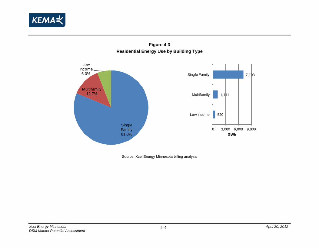
Xcel Energy Minnesota April 20, 2012
Single Family81.3%
Multifamily12.7%
Low Income6.0%
520
1,111
7,103
0 3,000 6,000 9,000
Low Income
Multifamily
Single Family
GWh
Source: Xcel Energy Minnesota billing analysis
Figure 4-3 Residential Energy Use by Building Type
DSM Market Potential Assessment 4–9

Xcel Energy Minnesota April 20, 2012 DSM Market Potential Assessment
4–10
Table 4-6 Residential Peak Demand by Building Type and End Use (MW)
Single Family Multifamily Low Income Total
Base Split-System Air Conditioner (11 SEER) 1,013 43 36 1,092 Base Early Replacement Split-System Air Conditioner (11 SEER) 224 9 8 241 Base Room Air Conditioner - EER 9.7 82 27 24 132 Base Early Replacement Room Air Conditioner- EER 9.0 15 5 4 25 Base Dehumidifier- New Federal Standard 7 1 1 8 Base Furnace Fans 105 4 7 116 Base Resistance Space Heating (Primary) 0 0 0 0 Base High-Efficiency Incandescent Lighting,<1.15 hrs/day 9 2 0 11 Base High-Efficiency Incandescent Lighting,1.15-2.15 hrs/day 38 7 2 46 Base High-Efficiency Incandescent Lighting,2.15-5 hrs/day 16 3 1 20 Base High-Efficiency Incandescent Lighting,>5 hrs/day 25 4 1 30 Base Lighting 15 Watt CFL, <1.15 hrs/day 0 0 0 0 Base Lighting 15 Watt CFL, 1.15-2.15 hrs/day 3 1 0 4 Base Lighting 15 Watt CFL, 2.15-5 hrs/day 3 0 0 4 Base Lighting 15 Watt CFL, >5 hrs/day 4 1 0 5 Base Fluorescent Fixture 1.8 hrs/day 16 1 1 18 Base Refrigerator 65 17 6 89 Base Early Replacement Refrigerator 12 3 1 16 Base Second Refrigerator 18 10 3 31 Base Freezer 18 8 2 27 Base Early Replacement Freezer 3 1 0 5 Base 40 gal. Water Heating (EF=0.88) 22 7 1 30 Base Early Replacement Water Heating to Heat Pump Water Heater 2 1 0 3 Base Clothes Washer (MEF=1.26) 7 2 1 10 Base Clothes Dryer (EF=3.01) 41 9 3 52 Base Dishwasher (EF=0.65) 11 5 1 18 Base Single Speed Pool Pump (RET) 0 0 0 0 Base Two Speed Pool Pump (1.5 hp) (ROB) 0 0 0 0 Base Plasma TV 2 1 0 3 Base LCD TV 10 3 1 13 Base CRT TV 13 3 1 17 Base Set-Top Box 15 4 1 21 Base DVD Player 3 1 0 3 Base Desktop PC 39 10 3 52 Base Laptop PC 11 3 0 15 Base Cooking 37 14 3 54 Base Miscellaneous 142 1 13 157 Base House Practices 1,924 301 141 2,366 Total 2,032 211 126 2,369
Source: KEMA analysis, calibrated to overall Xcel Energy peak load

Xcel Energy Minnesota April 20, 2012 DSM Market Potential Assessment
4–11
4.3 Commercial For this energy efficiency potential study, we broke the commercial sector into 12 segments, including small and large categories for office and retail buildings, with large defined as customers using more than 3,000,000 kWh per year.
We calculated equipment saturations (percent of households having an end use) from the results of the commercial onsite surveys. These are shown in Table 4-7.
Table 4-8 shows the end-use energy intensities for the commercial sector by base measure. End-use energy intensities represent the energy use per square foot for buildings that have that end-use.
Commercial floorspace is shown in Table 4-9 and energy use by building type and end-use is shown in Table 4-10. Figure 4-4 and Figure 4-5 show graphically the breakout of energy use by end-use and building type, respectively.
KEMA utilized load shape data from Xcel Energy to allocate annual energy usage to Xcel Energy’s time-of-use (TOU) periods. Peak-period usage, developed on a sector-specific and end-use basis, was calibrated to equal the Xcel Energy summer peak. Table 4-11shows the commercial peak electricity consumption results developed for the study.

Xcel Energy Minnesota April 20, 2012 DSM Market Potential Assessment
4–12
Table 4-7 Commercial Sector Equipment Saturations
End Use Office-S
Office-L
Restaurant Retail-S
Retail-L
Grocery Warehouse School College Health Lodging Other
Base Fluorescent Fixture, 4L4'T8 61% 57% 6% 35% 34% 85% 70% 39% 15% 49% 2% 24% Base Fluorescent Fixture, 2L4'T8, 1 EB 2% 1% 70% 12% 0% 0% 0% 4% 23% 12% 9% 22% Base Other Fluorescent Fixture 5% 1% 0% 0% 0% 0% 0% 1% 3% 4% 0% 1% Base High-Efficiency Incandescent Flood, 53W to Screw-in Replacement
1% 1% 15% 10% 0% 0% 0% 2% 16% 1% 2% 2%
Base High-Efficiency Incandescent Flood, 53W to Hardwired Replacement
1% 0% 54% 2% 0% 0% 0% 1% 6% 11% 7% 21%
Base CFL 3% 8% 7% 9% 0% 0% 0% 4% 10% 9% 64% 9% Base High Bay Metal Halide, 400W 0% 0% 16% 0% 24% 4% 2% 3% 0% 1% 2% 10% Base Parking Garage Metal Halide, 250 W 0% 44% 0% 0% 0% 0% 0% 0% 18% 7% 0% 0% Base Parking Garage Fluorescent 10% 32% 0% 0% 0% 0% 0% 0% 0% 0% 2% 7% Base Exit Sign 82% 100% 79% 42% 100% 99% 100% 100% 100% 100% 100% 98% Base Outdoor High Pressure Sodium 250W Lamp
42% 35% 100% 45% 100% 99% 43% 93% 52% 93% 74% 87%
Base Streetlighting High Pressure Sodium 0% 0% 0% 0% 0% 0% 0% 0% 0% 0% 0% 100% Base Centrifugal Chiller, 0.58 kW/ton, 500 tons 0% 67% 0% 7% 0% 42% 0% 30% 23% 30% 39% 11% Base DX Packaged System, EER=10.3, 10 tons
39% 18% 85% 46% 135% 54% 19% 57% 44% 62% 19% 48%
Base PTAC, EER=8.3, 1 ton 0% 0% 0% 0% 0% 0% 0% 0% 0% 0% 25% 16% Base Fan Motor, 5hp, 1800rpm, 87.5% 42% 48% 50% 43% 100% 97% 30% 33% 82% 19% 65% 54% Base Fan Motor, 15hp, 1800rpm, 91.0% 7% 21% 0% 2% 0% 0% 0% 89% 69% 65% 0% 43% Base Fan Motor, 40hp, 1800rpm, 93.0% 5% 36% 0% 2% 0% 96% 10% 37% 69% 69% 11% 34% Base Built-Up Refrigeration System 0% 1% 38% 0% 10% 11% 3% 8% 1% 1% 2% 0% Base Self-Contained Refrigeration 2% 0% 40% 5% 100% 100% 0% 57% 0% 5% 41% 1% Base Desktop PC 100% 84% 95% 62% 100% 97% 100% 93% 99% 92% 100% 96% Base Monitor, CRT 24% 0% 27% 29% 41% 2% 92% 75% 36% 67% 27% 38% Base Monitor, LCD 100% 57% 95% 62% 100% 97% 100% 93% 99% 92% 100% 100% Base Copier 87% 57% 70% 53% 100% 97% 99% 92% 68% 88% 95% 88% Base Laser Printer 84% 25% 25% 29% 100% 2% 95% 88% 51% 92% 100% 86%

Xcel Energy Minnesota April 20, 2012 DSM Market Potential Assessment
4–13
Table 4-7 Commercial Sector Equipment Saturations
End Use Office-S
Office-L
Restaurant Retail-S
Retail-L
Grocery Warehouse School College Health Lodging Other
Base Data Center/Server Room 0.3% 0.1% 0.0% 0.0% 0.0% 0.1% 0.0% 0.0% 0.1% 0.2% 0.0% 0% Base Water Heating 51% 65% 17% 34% 0% 5% 63% 11% 3% 0% 0% 32% Base Vending Machines 100% 69% 24% 100% 100% 100% 73% 83% 37% 88% 18% 69% Base Cooking 2% 31% 67% 7% 75% 97% 0% 90% 30% 22% 33% 6% Base Heating 0% 32% 7% 2% 0% 0% 0% 0% 0% 0% 33% 1% Base Miscellaneous 100% 100% 100% 100% 100% 100% 100% 100% 100% 100% 100% 100%
Source: Commercial on-site survey data

Xcel Energy Minnesota April 20, 2012 DSM Market Potential Assessment
4-14
Table 4-8 Commercial End-Use Energy Intensities (kWh per End-Use Square Foot)
Office-S
Office-L
Restaurant Retail-S
Retail-L
Grocery Warehouse School College Health Lodging Other
Base Fluorescent Fixture, 4L4'T8 8.0 7.8 6.8 3.7 3.4 7.5 1.6 3.2 8.5 5.6 1.8 2.6 Base Fluorescent Fixture, 2L4'T8, 1 EB 4.6 4.6 3.0 2.2 3.1 6.2 1.4 2.2 5.3 2.7 1.3 2.1 Base Other Fluorescent Fixture 3.6 1.7 0.0 1.0 0.0 0.0 2.1 0.4 2.2 2.1 0.6 0.5 Base High-Efficiency Incandescent Flood, 53W to Screw-in Replacement
24.3 6.8 3.0 3.9 10.4 5.1 0.0 0.2 4.3 2.7 3.6 3.1
Base High-Efficiency Incandescent Flood, 53W to Hardwired Replacement
24.3 0.0 3.0 3.9 0.0 5.1 2.8 0.2 4.3 2.7 3.6 3.1
Base CFL 1.4 2.3 0.8 0.6 0.0 6.3 0.7 1.3 1.3 0.9 0.6 0.6 Base High Bay Metal Halide, 400W 0.0 4.7 0.1 0.0 3.3 11.0 1.2 3.3 13.5 0.0 2.0 1.1 Base Parking Garage Metal Halide, 250 W 0.0 3.0 0.0 0.0 0.0 0.0 0.0 0.0 0.1 0.4 0.0 0.0 Base Parking Garage fluorescent 0.2 0.2 0.0 0.0 0.0 0.0 0.0 0.0 0.0 0.0 0.4 0.7 Base Exit Sign 0.0 0.0 0.1 0.0 0.0 0.0 0.0 0.0 0.0 0.0 0.0 0.0 Base Outdoor Metal Halide 295W Lamp 1.0 0.2 3.6 1.2 0.5 0.4 0.6 0.8 0.7 0.4 0.4 0.4 Base Street Lighting High Pressure Sodium 0.0 0.0 0.0 0.0 0.0 0.0 0.0 0.0 0.0 0.0 0.0 0.7 Base Centrifugal Chiller, 0.58 kW/ton, 500 tons 2.9 2.9 3.8 2.3 0.9 1.7 1.0 0.9 1.7 3.1 0.9 0.9 Base DX Packaged System, EER=10.3, 10 tons 4.9 4.9 6.7 4.0 1.6 2.9 1.7 1.5 2.9 5.3 1.6 1.6 Base PTAC, EER=8.3, 1 ton 0.0 0.0 0.0 0.0 0.0 0.0 0.0 1.6 2.9 0.0 1.8 1.4 Base Fan Motor, 5hp, 1800rpm, 87.5% 2.4 3.2 6.1 4.1 1.9 1.1 0.7 0.6 1.0 2.0 2.7 0.6 Base Fan Motor, 15hp, 1800rpm, 91.0% 2.2 2.9 5.6 3.8 1.8 1.0 0.6 0.6 0.9 1.9 2.5 0.6 Base Fan Motor, 40hp, 1800rpm, 93.0% 2.2 2.9 5.5 3.7 1.7 1.0 0.6 0.6 0.9 1.9 2.5 0.6 Base Built-Up Refrigeration System 13.0 0.4 7.0 8.0 1.6 16.2 18.0 0.3 0.5 0.7 0.8 2.0 Base Self-Contained Refrigeration 0.1 0.1 4.5 3.1 3.0 2.4 0.1 0.2 0.2 0.2 0.2 0.1 Base Desktop PC 1.2 1.8 0.3 0.1 0.1 0.1 0.2 0.2 0.1 0.7 0.0 0.1 Base Monitor, CRT 0.0 0.0 0.0 0.0 0.0 0.0 0.0 0.0 0.0 0.0 0.0 0.0 Base Monitor, LCD 0.4 0.5 0.1 0.0 0.0 0.0 0.1 0.1 0.0 0.2 0.0 0.0 Base Copier 0.0 0.1 0.0 0.0 0.0 0.0 0.0 0.0 0.0 0.1 0.0 0.0 Base Laser Printer 0.2 0.1 0.0 0.0 0.0 0.0 0.0 0.0 0.0 0.1 0.0 0.0 Base Data Center/Server Room 236.0 236.0 265.8 282.2 282.2 407.5 25.9 94.6 75.2 118.3 194.9 116.2

Xcel Energy Minnesota April 20, 2012 DSM Market Potential Assessment
4-15
Table 4-8 Commercial End-Use Energy Intensities (kWh per End-Use Square Foot)
Office-S
Office-L
Restaurant Retail-S
Retail-L
Grocery Warehouse School College Health Lodging Other
Base Water Heating 0.4 0.2 2.2 0.3 0.3 0.5 0.1 0.2 0.2 0.4 1.0 0.4 Base Vending Machines 0.1 0.1 0.1 0.1 0.1 0.2 0.1 0.1 0.1 0.1 0.1 0.0 Base Cooking 0.1 0.1 10.4 0.3 0.3 1.6 0.0 0.2 0.3 0.4 0.7 0.3 Base Heating 0.4 1.6 0.7 11.1 0.4 0.6 10.2 0.2 10.4 1.0 1.5 10.0 Base Miscellaneous 1.0 0.7 1.4 0.8 0.8 0.7 0.4 0.3 0.5 2.5 1.1 1.1
Source: Various sources, calibrated to estimates of overall building energy intensity per square foot.

Xcel Energy Minnesota April 20, 2012 DSM Market Potential Assessment
4-16
Table 4-9 Commercial Sector Floorspace (1000 sf) by Building Type
Office-S Office-L Restau-rant
Retail-S Retail-L
Grocery Ware-house
School College Health Lodging Other Total
Floorspace (1000 sf) 235,208 171,167 21,851 157,204 40,659 34,749 359,597 106,866 34,360 31,790 55,723 214,634 1,463,808
Source: KEMA analysis
Table 4-10 Commercial Sector Energy Use (MWh) by End-Use and Building Type
Office-S Office-L Restau-rant
Retail-S Retail-L Grocery Ware-house
School College Health Lodging Other Total
Base Fluorescent Fixture, 4L4'T8 1,148,900 756,385 8,330 204,417 46,766 221,859 393,477 136,257 43,760 87,238 1,497 134,666 3,183,553
Base Fluorescent Fixture, 2L4'T8, 1 EB 19,208 4,585 46,043 40,736 433 775 2,596 8,529 40,874 10,668 6,156 100,297 280,898
Base Other Fluorescent Fixture 41,041 1,783 0 294 0 0 367 678 2,017 2,822 118 1,280 50,400
Base High-Efficiency Incandescent Flood, 53W to Screw-in Replacement 68,936 6,774 9,971 60,106 1,464 157 0 390 24,417 1,100 3,334 11,981 188,631
Base High-Efficiency Incandescent Flood, 53W to Hardwired Replacement 32,599 0 35,721 12,308 0 477 5,061 194 9,078 9,338 13,753 139,680 258,210
Base CFL 8,851 32,170 1,142 9,192 0 506 67 5,793 4,416 2,583 22,494 11,170 98,385
Base High Bay Metal Halide, 400W 0 1,665 237 0 32,120 14,844 8,688 10,369 584 0 2,561 21,849 92,916
Base Parking Garage Metal Halide, 250 W 0 226,267 0 0 0 0 0 0 688 935 0 0 227,890
Base Parking Garage Fluorescent 3,798 11,505 0 0 0 0 0 0 0 0 418 9,212 24,931
Base Exit Sign 2,889 2,550 1,005 966 591 379 1,388 1,125 776 862 1,388 653 14,572
Base Outdoor High Pressure Sodium 250W Lamp 102,310 9,277 78,714 84,907 21,978 14,889 85,831 78,158 13,072 11,166 15,070 72,944 588,316
Base Street Lighting High Pressure Sodium 0 0 0 0 0 0 0 0 0 0 0 141,146 141,146
Base Centrifugal Chiller, 0.58 kW/ton, 500 tons 0 325,084 0 26,818 0 24,575 703 27,520 13,145 28,823 20,058 21,659 488,384
Base DX Packaged System, EER=10.3, 10 tons 452,042 150,049 123,607 293,428 85,163 55,366 115,833 90,600 44,544 104,274 16,756 161,142 1,692,805
Base PTAC, EER=8.3, 1 ton 0 0 0 0 0 0 0 547 266 0 25,209 49,900 75,921
Base Fan Motor, 5hp, 1800rpm, 87.5% 236,615 257,726 66,769 276,043 76,867 35,349 72,461 22,073 28,618 12,252 100,040 69,501 1,254,315

Xcel Energy Minnesota April 20, 2012 DSM Market Potential Assessment
4-17
Table 4-10 Commercial Sector Energy Use (MWh) by End-Use and Building Type
Office-S Office-L Restau-rant
Retail-S Retail-L Grocery Ware-house
School College Health Lodging Other Total
Base Fan Motor, 15hp, 1800rpm, 91.0% 38,001 102,723 0 8,917 0 0 0 54,770 22,367 39,475 0 51,358 317,610
Base Fan Motor, 40hp, 1800rpm, 93.0% 23,560 175,482 0 8,769 0 31,861 21,909 22,452 21,996 41,249 15,766 40,079 403,124
Base Built-Up Refrigeration System 3,455 793 58,585 6,125 6,587 60,031 191,464 2,465 152 247 907 270 331,082
Base Self-Contained Refrigeration 776 0 39,800 26,369 121,247 83,365 0 11,170 0 367 4,736 295 288,125
Base Desktop PC 272,332 256,373 5,383 6,888 2,574 1,781 68,275 23,910 2,799 20,061 2,329 16,127 678,832
Base Monitor, CRT 544 0 120 160 207 8 4,228 190 131 805 71 0 6,466
Base Monitor, LCD 105,818 51,434 1,772 3,117 698 513 20,252 6,286 769 5,914 632 4,562 201,767
Base Copier 8,017 7,147 724 1,637 293 524 7,211 489 102 1,645 196 1,324 29,308
Base Laser Printer 32,143 3,588 119 1,225 667 6 9,192 1,226 157 2,335 458 2,206 53,323
Base Data Center/Server Room 185,733 23,009 1,002 7,996 4,126 9,596 2,090 838 1,876 8,001 2,447 132 246,845
Base Water Heating 49,182 26,702 8,246 13,362 0 886 15,285 2,469 247 0 0 24,039 140,419
Base Vending Machines 13,459 10,771 745 16,106 5,537 5,715 24,085 11,277 1,495 1,619 1,166 6,094 98,068
Base Cooking 582 6,408 153,435 3,029 7,952 53,090 0 17,283 3,332 3,019 13,272 3,580 264,982
Base Heating 0 89,355 1,134 29,776 0 0 13,475 0 808 0 27,855 11,377 173,779
Base Miscellaneous 232,856 111,258 30,373 125,764 32,527 25,839 157,471 27,785 17,180 80,747 62,410 231,805 1,136,014
Total 3,083,648 2,650,863 672,975 1,268,455 447,797 642,391 1,221,409 564,846 299,664 477,545 361,099 1,340,327 13,031,018
Source: KEMA analysis, calibrated to overall energy use by building type from the analysis of Xcel Energy’s billing data

Xcel Energy Minnesota April 20, 2012
Figure 4-4 Commercial Energy Use by End-Use
Indoor Lighting33.8%
Cooling17.3%
Ventilation15.2%
Off ice Equip9.3%
Miscellaneous
8.8%
Outdoor Lightng5.6%
Refrigeration4.8% Cooking-
Vending2.8%
Heating1.3%
Water Heating
1.1%
140
174
363
619
729
1,151
1,217
1,975
2,257
4,406
0 2,000 4,000 6,000
Water Heating
Heating
Cooking-Vending
Refrigeration
Outdoor Lightng
Miscellaneous
Off ice Equip
Ventilation
Cooling
Indoor Lighting
GWh
Source: KEMA analysis, calibrated to total commercial energy use
DSM Market Potential Assessment 4-18

Xcel Energy Minnesota April 20, 2012
Figure 4-5 Commercial Energy Use by Building Type
Off ice-S23.7%
Off ice-L20.3%
Com Misc
10.3%Retail-S
9.7%Warehouse
9.4%
Restaurant5.2%
Grocery4.9%
School4.3%
Health3.7%
Retail-L3.4%
Lodging2.8% College
2.3%
300
361
448
478
565
642
673
1,221
1,268
1,340
2,651
3,084
0 1,000 2,000 3,000 4,000
College
Lodging
Retail-L
Health
School
Grocery
Restaurant
Warehouse
Retail-S
Com Misc
Of f ice-L
Off ice-S
GWh
Source: Xcel Energy Minnesota billing analysis
DSM Market Potential Assessment 4-19
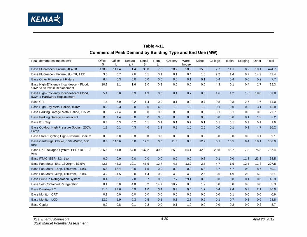
Xcel Energy Minnesota April 20, 2012 DSM Market Potential Assessment
4-20
Table 4-11 Commercial Peak Demand by Building Type and End Use (MW)
Peak demand estimates MW Office-S
Office-L
Restau-rant
Retail-S
Retail-L
Grocery Ware-house
School College Health Lodging Other Total
Base Fluorescent Fixture, 4L4'T8 178.3 117.4 1.4 30.8 7.0 28.2 58.0 15.6 7.7 11.1 0.2 19.1 474.7 Base Fluorescent Fixture, 2L4'T8, 1 EB 3.0 0.7 7.6 6.1 0.1 0.1 0.4 1.0 7.2 1.4 0.7 14.2 42.4 Base Other Fluorescent Fixture 6.4 0.3 0.0 0.0 0.0 0.0 0.1 0.1 0.4 0.4 0.0 0.2 7.7 Base High-Efficiency Incandescent Flood, 53W to Screw-in Replacement
10.7 1.1 1.6 9.0 0.2 0.0 0.0 0.0 4.3 0.1 0.4 1.7 29.3
Base High-Efficiency Incandescent Flood, 53W to Hardwired Replacement
5.1 0.0 5.9 1.9 0.0 0.1 0.7 0.0 1.6 1.2 1.6 19.8 37.8
Base CFL 1.4 5.0 0.2 1.4 0.0 0.1 0.0 0.7 0.8 0.3 2.7 1.6 14.0 Base High Bay Metal Halide, 400W 0.0 0.3 0.0 0.0 4.8 1.9 1.3 1.2 0.1 0.0 0.3 3.1 13.0 Base Parking Garage Metal Halide, 175 W 0.0 27.4 0.0 0.0 0.0 0.0 0.0 0.0 0.1 0.1 0.0 0.0 27.7 Base Parking Garage Fluorescent 0.5 1.4 0.0 0.0 0.0 0.0 0.0 0.0 0.0 0.0 0.1 1.3 3.2 Base Exit Sign 0.4 0.3 0.2 0.1 0.1 0.1 0.2 0.1 0.1 0.1 0.2 0.1 1.9 Base Outdoor High Pressure Sodium 250W Lamp
1.2 0.1 4.3 4.6 1.2 0.3 1.0 2.6 0.0 0.1 0.1 4.7 20.2
Base Street Lighting High Pressure Sodium 0.0 0.0 0.0 0.0 0.0 0.0 0.0 0.0 0.0 0.0 0.0 9.1 9.1 Base Centrifugal Chiller, 0.58 kW/ton, 500 tons
0.0 110.6 0.0 12.5 0.0 11.5 0.3 12.9 6.1 13.5 9.4 10.1 186.9
Base DX Packaged System, EER=10.3, 10 tons
226.6 51.0 57.8 137.2 39.8 25.9 54.1 42.3 20.8 48.7 7.8 75.3 787.4
Base PTAC, EER=8.3, 1 ton 0.0 0.0 0.0 0.0 0.0 0.0 0.0 0.3 0.1 0.0 11.8 23.3 35.5 Base Fan Motor, 5hp, 1800rpm, 87.5% 42.5 46.3 10.1 45.5 12.7 4.5 13.2 2.5 4.7 1.5 12.5 11.8 207.8 Base Fan Motor, 15hp, 1800rpm, 91.0% 6.8 18.4 0.0 1.5 0.0 0.0 0.0 6.3 3.7 4.7 0.0 8.7 50.1 Base Fan Motor, 40hp, 1800rpm, 93.0% 4.2 31.5 0.0 1.4 0.0 4.0 4.0 2.6 3.6 4.9 2.0 6.8 65.1 Base Built-Up Refrigeration System 0.4 0.1 7.0 0.7 0.8 7.7 29.1 0.3 0.0 0.0 0.1 0.0 46.3 Base Self-Contained Refrigeration 0.1 0.0 4.8 3.2 14.7 10.7 0.0 1.2 0.0 0.0 0.6 0.0 35.3 Base Desktop PC 31.5 29.6 0.9 1.0 0.4 0.3 9.5 1.7 0.4 2.4 0.3 2.1 80.0 Base Monitor, CRT 0.1 0.0 0.0 0.0 0.0 0.0 0.6 0.0 0.0 0.1 0.0 0.0 0.9 Base Monitor, LCD 12.2 5.9 0.3 0.5 0.1 0.1 2.8 0.5 0.1 0.7 0.1 0.6 23.8 Base Copier 0.9 0.8 0.1 0.2 0.0 0.1 1.0 0.0 0.0 0.2 0.0 0.2 3.7

Xcel Energy Minnesota April 20, 2012 DSM Market Potential Assessment
4-21
Table 4-11 Commercial Peak Demand by Building Type and End Use (MW)
Peak demand estimates MW Office-S
Office-L
Restau-rant
Retail-S
Retail-L
Grocery Ware-house
School College Health Lodging Other Total
Base Laser Printer 3.7 0.4 0.0 0.2 0.1 0.0 1.3 0.1 0.0 0.3 0.1 0.3 6.4 Base Data Center/Server Room 21.5 2.7 0.2 1.2 0.6 1.4 0.3 0.1 0.3 0.9 0.3 0.0 29.4 Base Water Heating 5.5 3.0 1.2 1.8 0.0 0.1 2.0 0.2 0.0 0.0 0.0 3.0 16.8 Base Vending Machines 1.6 1.3 0.1 2.4 0.8 0.8 3.8 0.8 0.2 0.2 0.2 0.8 13.1 Base Cooking 0.1 0.8 26.2 0.5 1.2 6.1 0.0 1.1 0.6 0.5 2.3 0.5 39.7 Base Heating 0.0 5.1 0.0 0.2 0.0 0.0 0.0 0.0 0.1 0.0 0.7 0.3 6.2 Base Miscellaneous 28.2 13.5 5.0 18.7 4.8 3.4 24.7 2.1 2.7 9.4 8.4 32.2 153.1 Total 592.7 475.0 134.7 282.7 89.6 107.2 208.3 96.1 65.9 102.7 62.6 251.0 2,468.5
Source: KEMA analysis, calibrated to overall Xcel Energy peak demand

Xcel Energy Minnesota April 20, 2012 DSM Market Potential Assessment
4-22
4.4 Industrial We broke out the share of energy use by industry and end use using the results of the industrial on-site surveys. Due to the small sample size at the industry level, these were calculated based on a breakdown of industries into assembly and process industries. These results were used to calibrate industry-level estimates from the Department of Energy’s Manufacturing End Use Consumption Survey (MECS). The results of this analysis are shown in Table 4-12.
We applied these breakout percents to energy use by industry from the billing analysis to obtain energy use by end-use and industry, shown in Table 4-13. Industrial energy use by end-use and by industry are shown in Figure 4-6 and Figure 4-7, respectively.

Xcel Energy Minnesota April 20, 2012 DSM Market Potential Assessment
4-23
Table 4-12 Percent of Industrial Energy Use by Industry and End-Use
Compressed Air
Fans Pumps Drives Process Heating
Process Cooling
Other Process
Chiller DX Lighting Other Total
Food 7% 26% 8% 18% 8% 20% 1% 0% 2% 5% 5% 100% Textiles 10% 9% 7% 30% 11% 10% 2% 0% 5% 14% 2% 100% Wood 4% 23% 5% 43% 8% 1% 1% 0% 1% 5% 9% 100% Paper 3% 36% 11% 32% 10% 1% 2% 0% 1% 2% 2% 100% Printing 11% 10% 7% 33% 4% 5% 1% 0% 7% 16% 6% 100% Chemicals 8% 9% 21% 21% 10% 7% 15% 0% 2% 5% 2% 100% Petroleum 12% 25% 30% 18% 6% 5% 1% 0% 1% 2% 2% 100% Plastics 10% 9% 7% 31% 16% 7% 2% 0% 4% 11% 3% 100% Stone, Clay, Glass 4% 36% 8% 21% 18% 2% 3% 0% 1% 3% 3% 100% Prim Metals 9% 10% 7% 10% 27% 1% 31% 0% 1% 4% 1% 100% Fab Metals 29% 8% 6% 18% 17% 2% 4% 0% 3% 10% 2% 100% Ind Mach 36% 6% 5% 15% 6% 2% 2% 0% 6% 16% 4% 100% Electronics 28% 4% 3% 8% 15% 7% 8% 0% 8% 14% 6% 100% Transp Equip 32% 7% 5% 10% 13% 5% 3% 0% 6% 16% 4% 100% Misc. 15% 10% 9% 42% 9% 6% 0% 0% 4% 5% 0% 100% WWTP 0% 41% 57% 0% 1% 0% 0% 0% 0% 1% 0% 100%
Source: Billing data analysis, on-site survey results, and Department of Energy’s Manufacturer Energy Consumption Survey data

Xcel Energy Minnesota April 20, 2012 DSM Market Potential Assessment
4-24
Table 4-13 Industrial Energy Use by Industry and End-Use
Compressed Air
Fans Pumps Drives Process Heating
Process Cooling
Other Process
Chiller DX Lighting Other Total
Food 67,745 251,375 78,786 173,443 81,719 199,069 11,319 0 19,448 49,216 52,705 984,825 Textiles 2,808 2,512 1,863 8,058 2,846 2,620 421 77 1,248 3,663 659 26,774 Wood 5,886 37,770 8,822 72,704 13,457 1,502 1,328 0 2,231 8,200 15,544 167,443 Paper 10,251 141,122 41,830 125,922 37,229 3,892 7,542 0 3,192 8,433 9,062 388,477 Printing 41,816 37,403 27,183 123,597 14,240 19,119 3,129 1,536 24,834 61,047 22,366 376,269 Chemicals 45,423 54,447 122,443 123,598 56,245 39,989 90,266 746 12,069 28,636 12,553 586,416 Petroleum 131,636 267,768 317,949 194,258 60,126 49,902 7,584 0 9,836 18,669 16,732 1,074,461 Plastics 46,004 41,148 29,905 135,975 71,038 33,051 7,802 999 16,156 49,108 13,676 444,860 Stone, Clay, Glass 10,139 80,781 18,265 47,460 41,801 3,973 7,225 0 2,759 6,606 7,230 226,240 Prim Metals 28,003 31,097 21,879 31,364 85,312 2,243 97,210 210 3,389 13,231 2,848 316,786 Fab Metals 88,688 23,343 16,965 54,315 50,790 7,400 12,585 533 8,628 30,794 6,743 300,784 Ind Mach 185,506 31,740 23,067 78,194 30,636 10,174 11,296 2,040 32,993 82,182 21,933 509,760 Electronics 124,115 17,772 12,916 34,924 63,793 29,894 33,646 2,082 33,664 62,426 24,287 439,520 Transp Equip 41,774 8,838 6,423 13,335 16,762 5,969 4,047 462 7,474 21,736 4,953 131,773 Misc. 64,398 42,352 37,238 181,335 38,197 26,617 0 474 18,535 21,876 0 431,022 WWTP 160 33,864 47,045 0 416 99 0 18 134 463 0 82,200 Total 894,352 1,103,331 812,579 1,398,481 664,607 435,512 295,399 9,177 196,591 466,288 211,293 6,487,611
Source: KEMA analysis, calibrated to Xcel Energy total industrial energy use by building type from billing analysis

Xcel Energy Minnesota April 20, 2012
Figure 4-6 Industrial Energy Use by End-Use
Drives 21.6%
Fans 17.0%
Compressed
Pumps 12.5%
Process Heating 10.2%
Lighting 7.2%
Refrigeration 6.7%
Other Process
4.6%
Other 3.3%
Cooling 3.2%
Air 13.8%
206211
295436466
665813
8941,103
1,398
0 500 1,000 1,500
Cooling
OtherOther Process
Refrigeration
LightingProcess Heating
PumpsCompressed Air
Fans
Drives
GWh
Source: On-site survey results and Department of Energy’s Manufacturer Energy Consumption Survey data
DSM Market Potential Assessment 4-25

Xcel Energy Minnesota April 20, 2012
Figure 4-7 Industrial Energy Use by Industry
Petroleum 16.6%
Food 15.2%
Chemicals 9.0%
Ind Mach Electronics
Misc. 6.6%
Paper 6.0%
Printing 5.8%
Prim Metals 4.9%
Fab Metals 4.6%
Stone,Clay,Glass
3.5%
Wood 2.6%
Transp Equip 2.0%
WWTP 1.3% Textiles
0.4%
7.9%Plastics 6.9%
6.8%
27
82
132
167
226
301
317
376
388
431
440
445
510
586
985
1,074
0 200 400 600 800 1,000 1,200
Textiles
WWTP
Transp Equip
Wood
Stone,Clay,Glass
Fab Metals
Prim Metals
Printing
Paper
Misc.
Electronics
Plastics
Ind Mach
Chemicals
Food
Petroleum
GWh
Source: Xcel Energy Minnesota billing analysis
DSM Market Potential Assessment 4-26

Xcel Energy Minnesota April 20, 2012 DSM Market Potential Assessment
4-27
Table 4-14 Industrial Peak Demand by Industry and End-Use (MW)
Compressed Air
Fans Pumps Drives Process Heating
Process Cooling
Other Process
Chiller DX Lighting Other Total
Food 8.0 29.6 9.3 20.4 9.6 23.5 1.3 0.0 2.3 5.8 6.2 116.1 Textiles 1.1 1.0 0.8 3.2 1.1 1.1 0.2 0.0 0.5 1.5 0.3 10.8 Lumber 0.9 5.5 1.3 10.6 2.0 0.2 0.2 0.0 0.3 1.2 2.3 24.3 Paper 0.8 11.0 3.3 9.8 2.9 0.3 0.6 0.0 0.2 0.7 0.7 30.3 Printing 5.4 4.8 3.5 15.8 1.8 2.4 0.4 0.2 3.2 7.8 2.9 48.2 Chemicals 5.0 6.1 13.6 13.7 6.3 4.4 10.0 0.1 1.3 3.2 1.4 65.2 Petroleum 14.6 29.8 35.3 21.6 6.7 5.5 0.8 0.0 1.1 2.1 1.9 119.4 Plastics 6.2 5.5 4.0 18.3 9.6 4.4 1.1 0.1 2.2 6.6 1.8 59.9 Stone-clay-glass 1.1 8.8 2.0 5.2 4.6 0.4 0.8 0.0 0.3 0.7 0.8 24.7 Primary Metals 3.9 4.3 3.0 4.4 11.9 0.3 13.5 0.0 0.5 1.8 0.4 44.1 Fab Metals 12.0 3.2 2.3 7.3 6.9 1.0 1.7 0.1 1.2 4.2 0.9 40.6 Ind Machinery 40.1 6.9 5.0 16.9 6.6 2.2 2.4 0.4 7.1 17.8 4.7 110.2 Electronics 15.4 2.2 1.6 4.3 7.9 3.7 4.2 0.3 4.2 7.7 3.0 54.5 Transp Equip 5.6 1.2 0.9 1.8 2.2 0.8 0.5 0.1 1.0 2.9 0.7 17.7 Misc 7.1 4.7 4.1 19.9 4.2 2.9 0.0 0.1 2.0 2.4 0.0 47.4 WWT 0.0 3.7 5.2 0.0 0.0 0.0 0.0 0.0 0.0 0.1 0.0 9.0 Total 127.2 128.2 95.1 173.4 84.3 53.3 37.8 1.4 27.5 66.4 27.9 822.5
Source: KEMA analysis, calibrated to overall Xcel Energy peak demand

Xcel Energy Minnesota April 20, 2012 DSM Market Potential Assessment
4-28
4.5 Opt-Out Analysis The analysis above was the basis for the potential analysis presented in this report. Xcel Energy requested that KEMA also look at the potential impacts of additional customers opting out of Minnesota’s Resource Adjustment Rider under the Omnibus Energy Policy bill. The bill exempts customers with electric demand over 20 MW or gas use over 500,000 Dth. These customers can elect to opt out of the rider and in doing so would be ineligible for any Xcel Energy energy efficiency or demand response programs.
The analysis above already excludes existing opt-out customers; however, Xcel Energy was concerned about the impact of potential additional customers opting out. KEMA reanalyzed the billing data, omitting customers identified by Xcel Energy as being exempt, or possibly exempt, from the rider. The result was a change in the building stock for the industrial sector, but no change to saturations or EUIs. This section presents the results of that analysis.
Table 4-15 compares the results of the nonresidential billing analysis for all nonresidential customers, nonresidential customers minus the current opt outs, and finally nonresidential customers minus existing and potential new opt outs.

Xcel Energy Minnesota April 20, 2012 DSM Market Potential Assessment
4-29
Table 4-15 Results of Nonresidential Billing Analysis with and without Likely Opt-Outs
All Customers Minus existing Opt-outs Minus existing and potential opt-outs
Sector Business Type Accounts kWh Accounts kWh Accounts kWh
AG Agriculture 2,278 121,456,178 2,278 121,456,178 2,278 121,456,178
COM College 733 299,663,809 733 299,663,809 733 299,663,809
COM Com misc 8,543 1,199,180,803 8,543 1,199,180,803 8,543 1,199,180,803
COM Grocery 1,859 642,391,389 1,859 642,391,389 1,859 642,391,389
COM Health 701 477,545,281 701 477,545,281 701 477,545,281
COM Lodging 898 361,098,555 898 361,098,555 898 361,098,555
COM Office-L 271 2,650,863,075 271 2,650,863,075 271 2,650,863,075
COM Office-S 47,250 3,083,647,936 47,250 3,083,647,936 47,250 3,083,647,936
COM Restaurant 4,715 672,974,975 4,715 672,974,975 4,715 672,974,975
COM Retail-L 91 447,797,056 91 447,797,056 91 447,797,056
COM Retail-S 14,273 1,268,454,809 14,273 1,268,454,809 14,273 1,268,454,809
COM School 1,377 564,845,806 1,377 564,845,806 1,377 564,845,806
COM Warehouse 6,642 1,221,408,759 6,642 1,221,408,759 6,642 1,221,408,759
CST Construction 5,937 299,645,047 5,937 299,645,047 5,937 299,645,047
IND Chemicals 305 586,415,802 305 586,415,802 293 523,660,664
IND Electronics 481 439,520,166 481 439,520,166 481 439,520,166
IND Fabricated metals 648 300,783,758 648 300,783,758 648 300,783,758
IND Food 485 984,825,485 485 984,825,485 485 984,825,485
IND Ind machinery 1,198 509,760,023 1,198 509,760,023 1,198 509,760,023
IND Ind misc 948 431,021,652 948 431,021,652 948 431,021,652
IND Paper 175 399,082,548 168 388,476,763 168 388,476,763
IND Petroleum 55 1,079,088,762 41 1,074,460,742 40 37,104,895
IND Plastics 378 444,860,498 378 444,860,498 378 444,860,498
IND Primary metals 184 563,765,842 173 316,786,010 173 316,786,010
IND Printing 940 376,268,923 940 376,268,923 940 376,268,923
IND Stone-clay-glass 260 226,240,094 260 226,240,094 260 226,240,094
IND Textiles 223 26,774,298 223 26,774,298 223 26,774,298
IND Transp equip 216 131,773,344 216 131,773,344 216 131,773,344
IND Wood 442 167,442,509 442 167,442,509 442 167,442,509
MIN Mining 127 56,024,350 127 56,024,350 127 56,024,350
TCU TCU 6,010 744,868,411 6,010 744,868,411 6,010 744,868,411
TCU Water-WWT 120 82,200,449 120 82,200,449 120 82,200,449
UNC Unclassified 12,610 586,111,213 12,610 586,111,213 12,610 586,111,213
Total 121,373 21,447,801,605 121,341 21,185,587,968 121,328 20,085,476,983

Xcel Energy Minnesota April 20, 2012 DSM Market Potential Assessment
4-30
The potential opt-outs are all industrial customers in the chemical and petroleum industries, so only those building types show a change from the current opt-out scenario to the current and potential opt-out scenario. Figure 4-8 and Figure 4-8 and compare industrial energy use with just the current opt-outs and with both the current and potential new opt-outs. The petroleum industry is dramatically affected, while the chemical industry has a much smaller change.
Figure 4-8 Comparison of Industrial Energy Use before and After Likely Opt-Outs
0 500 1,000 1,500
TextilesWater-WWT
Transp EquipWood
Stone-Clay-GlassFabricated Metals
Primary MetalsPrinting
PaperInd Misc
ElectronicsPlastics
Ind MachineryChemicals
FoodPetroleum
GWh
Minus current opt-outs
Minus current and new opt-outs

Xcel Energy Minnesota April 20, 2012
Figure 4-9 Industrial Energy Use by Industry with and without Likely Additional Opt-Out Customers
Textiles0.4%
Water-WWT1.3%
Transp Equip2.0% Wood
2.6%
Stone-Clay-Glass3.5%
Fabricated Metals4.6%
Primary Metals4.9%
Printing5.8%
Paper6.0%
Ind Misc6.6%
ElectronicsInd Machinery
Chemicals9.0%
Food15.2%
Petroleum16.6%
Industrial Minus Current Opt-Outs
6.8%Plastics6.9%7.9%
Textiles0.5%
Water-WWT1.5%
Transp Equip2.4%Wood
3.1%
Stone-Clay-Glass4.2%Fabricated
Metals5.6%
Primary Metals5.9%
Printing7.0%
Paper7.2%
Ind Misc8.0%
Plastics8.3%
Ind Machinery9.5%
Chemicals9.7%
Food18.3%
Petroleum0.7%
Industrial Minus Current and New Opt-Outs
Electronics8.2%
DSM Market Potential Assessment 4-31

Xcel Energy Minnesota April 20, 2012 DSM Market Potential Assessment
4-32
Table 4-16 shows the new building stock for the industrial sector after the potential additional opt outs.
Table 4-16 Industrial Building Stock for Opt-Out Analysis
Base Energy Use (kWh)
Food 912,252,445 Textiles 26,557,686 Wood 167,015,964 Paper 389,462,178 Printing 375,279,206 Chemicals 193,497,871 Petroleum 36,576,787 Plastics 439,621,890 Stone,Clay,Glass 144,886,780 Prim Metals 475,417,489 Fab Metals 295,426,049 Ind Mach 507,483,821 Electronics 438,973,482 Transp Equip 76,300,383 Misc. 420,602,887 WWTP 82,195,101 Total 4,981,550,019

Xcel Energy Minnesota April 20, 2012 DSM Market Potential Assessment
5-1
5. Electric Energy-Efficiency Potential Results
In this section, we present estimates of electric energy-efficiency potential. First, we present technical and economic potential results for all electric measures considered in the study. Next, we present estimates of achievable program potential under different program funding scenarios. The base energy-efficiency results exclude impacts from behavioral-conservation programs and from emerging technologies. These additional elements are discussed separately, since these measures do not have the track record of more proven energy-efficiency technologies, and their impacts are more uncertain.
5.1 Technical and Economic Potential Estimates of overall energy-efficiency technical and economic potential are discussed in section 5.1.1. More detail on these potentials is presented in section 5.1.2. Energy-efficiency supply curves are shown in section 5.1.3.
5.1.1 Overall Technical and Economic Potential
Figure 5-1 presents our overall estimates of total technical and economic potential for electrical energy and peak-demand savings for the Xcel Energy Minnesota service territory. Technical potential represents the sum of all savings from all of the measures deemed applicable and technically feasible. Economic potential is based on efficiency measures that are cost-effective, which is based on the total resource cost (TRC) test―a benefit-cost test that compares the value of avoided energy production and power-plant construction to the costs of energy-efficiency measures and program activities necessary to deliver them. The values of both energy savings and peak-demand reductions are incorporated in the TRC test.
Energy Savings. Technical potential is estimated at about 10,249 GWh per year, and economic potential at 7,164 GWh per year by 2020 (about 29 and 20 percent of base 2020 usage, respectively).
Peak-Demand Savings. Technical potential is estimated at about 1,972 MW, and economic potential at 1,415 MW by 2020 (about 27 and 19 percent of base 2020 demand, respectively).

Xcel Energy Minnesota April 20, 2012 DSM Market Potential Assessment
5-2
Figure 5-1 Estimated Electric Technical and Economic Potential, 2020
Xcel Energy Minnesota Service Territory
35,130 GWh
7,325 MW
10,249 GWh
1,972 MW
7,164 GWh
1,415 MW
0
5,000
10,000
15,000
20,000
25,000
30,000
35,000
40,000
Energy Savings Potential Peak Demand Savings Potential
2020 BaseTechnical PotentialEconomic Potential
5.1.2 Technical and Economic Potential Detail
In this subsection, we explore technical and economic potential in more detail, looking at potentials by sector and by end use.
5.1.2.1 Potentials by Sector
Figure 5-2 and Figure 5-3 show estimates of technical- and economic-energy and demand savings potential by sector. Figure 5-4 and Figure 5-5 show the same potentials as a percentage of 2020 base energy and base peak demand.
The commercial sector provides the largest contribution to both technical and economic potential for energy savings, accounting for just under 50 percent of these potentials. The residential sector contributes the most to the technical and economic potential for peak-demand savings, accounting for over 55 percent of these potentials. While the industrial sector contributes low amounts to the potentials, we note that industrial facilities typically contain complex custom measures that are difficult to completely capture in a bottom-up study such as this one, and this effect could lead to an understatement of industrial potentials.

Xcel Energy Minnesota April 20, 2012 DSM Market Potential Assessment
5-3
Figure 5-2 Technical and Economic Potential (2020)
Energy Savings by Sector—GWh per Year
Figure 5-3 Technical and Economic Potential (2020)
Demand Savings by Sector—MW
3,691
5,046
1,512
2,531
3,339
1,294
0
1,000
2,000
3,000
4,000
5,000
6,000
Residential Commercial Industrial
Cum
ulat
ive
Ann
ual S
avin
gs b
y 20
20-G
Wh Technical
Economic
1,094
713
165
807
467
141
0
200
400
600
800
1,000
1,200
Residential Commercial Industrial
Cum
ulat
ive
Savi
ngs
by 2
020
-MW
Technical
Economic
As shown in Figure 5-4 and Figure 5-5, the residential and commercial sectors have a similar savings potential in relation to base energy use. The estimated savings fraction is lowest for the industrial sector, but this potential is in the range of the 14 to 22 percent of cost-effective industrial savings estimated by the National Academy of Sciences3.
3 Real Prospects for Energy Efficiency in the United States, America’s Energy Future Energy Efficiency Subcommittee, Nation Academy of Sciences, National Academy of Engineering, National Research Council, 2009.

Xcel Energy Minnesota April 20, 2012 DSM Market Potential Assessment
5-4
Figure 5-4 Technical and Economic Potential (2020)
Percentage of Base Energy Use
Figure 5-5 Technical and Economic Potential (2020)
Percentage of Base Peak Demand
37%35%
21%
25%23%
18%
0%
5%
10%
15%
20%
25%
30%
35%
40%
Residential Commercial Industrial
Perc
ent o
f For
ecas
t Ene
rgy
Use
Technical
Economic
39%
25%
17%
29%
16%15%
0%
5%
10%
15%
20%
25%
30%
35%
40%
45%
Residential Commercial Industrial
Perc
ent o
f For
ecas
t Pea
k D
eman
d
Technical
Economic
5.1.2.2 Potentials by Building Type
Figure 5-6 and Figure 5-7 show the potentials in the residential sector by building type. Single-family homes account for about 84 percent of the economic potential, and low-income homes account for about 5 percent of the potential.
Figure 5-6 Residential Energy-Savings Potential by
Building Type (2020)
Figure 5-7 Residential Demand-Savings Potential by
Building Type (2020)
3,008
500
183
2,128
286
117
0 500 1,000 1,500 2,000 2,500 3,000 3,500
Single Family
Multifamily
Low Income
Cumulative Annual Savings by 2020 - GWh
Technical
Economic
949
96
49
726
48
33
0 200 400 600 800 1,000
Single Family
Multifamily
Low Income
Cumulative Peak Savings by 2020 - MW
Technical
Economic

Xcel Energy Minnesota April 20, 2012 DSM Market Potential Assessment
5-5
Figure 5-8 and Figure 5-9 show the building-type breakdown of commercial potential. Offices account for almost 60 percent of the economic energy savings potential, with small offices (office accounts under 3 GWh per year consumption) accounting for over 30 percent of total potential. The retail and restaurant segments account for the next largest shares of potential.
Figure 5-8 Commercial Economic Energy-Savings
Potential by Building Type (2014)
Figure 5-9 Commercial Economic Demand-Savings
Potential by Building Type (2014)
1,343
1,103
268
466
129
230
419
244
119
134
1,060
901
187
338
78
151
168
80
82
91
0 500 1,000 1,500
Office-S
Office-L
Restaurant
Retail-S
Retail-L
Grocery
Warehouse
School
College
Health
Cumulative Annual Savings by 2020 - GWh
Technical
Economic
185
133
45
83
21
29
54
28
20
25
143
103
36
59
10
21
20
10
14
19
0 50 100 150 200
Office-S
Office-L
Restaurant
Retail-S
Retail-L
Grocery
Warehouse
School
College
Health
Cumulative Peak Savings to 2020 - MW
Technical
Economic
Figure 5-10 and Figure 5-11 show the business-type breakdown of industrial potential. Key industries in terms of economic potential include food processing and petroleum refining, plastics, chemicals, industrial machinery, and electronics.
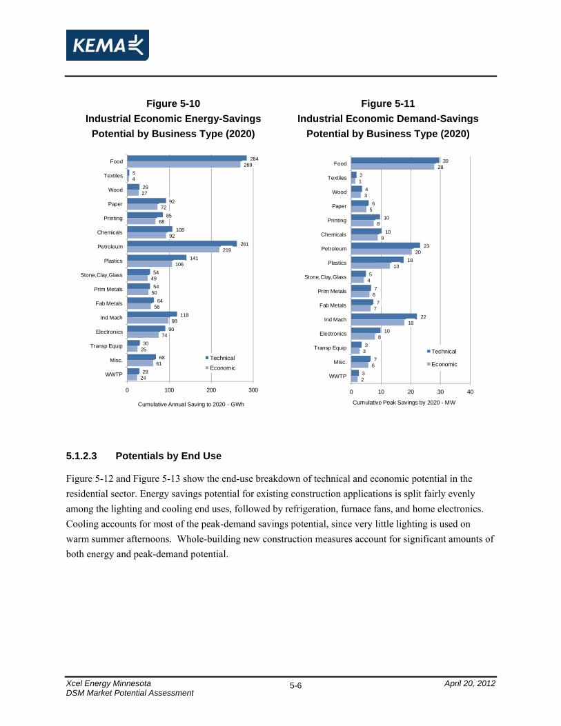
Xcel Energy Minnesota April 20, 2012 DSM Market Potential Assessment
5-6
Figure 5-10 Industrial Economic Energy-Savings
Potential by Business Type (2020)
Figure 5-11 Industrial Economic Demand-Savings
Potential by Business Type (2020)
284
5
29
92
85
108
261
141
54
54
64
118
90
30
68
29
269
4
27
72
68
92
219
106
49
50
56
98
74
25
61
24
0 100 200 300
Food
Textiles
Wood
Paper
Printing
Chemicals
Petroleum
Plastics
Stone,Clay,Glass
Prim Metals
Fab Metals
Ind Mach
Electronics
Transp Equip
Misc.
WWTP
Cumulative Annual Saving to 2020 - GWh
Technical
Economic
30
2
4
6
10
10
23
18
5
7
7
22
10
3
7
3
28
1
3
5
8
9
20
13
4
6
7
18
8
3
6
2
0 10 20 30 40
Food
Textiles
Wood
Paper
Printing
Chemicals
Petroleum
Plastics
Stone,Clay,Glass
Prim Metals
Fab Metals
Ind Mach
Electronics
Transp Equip
Misc.
WWTP
Cumulative Peak Savings by 2020 - MW
Technical
Economic
5.1.2.3 Potentials by End Use
Figure 5-12 and Figure 5-13 show the end-use breakdown of technical and economic potential in the residential sector. Energy savings potential for existing construction applications is split fairly evenly among the lighting and cooling end uses, followed by refrigeration, furnace fans, and home electronics. Cooling accounts for most of the peak-demand savings potential, since very little lighting is used on warm summer afternoons. Whole-building new construction measures account for significant amounts of both energy and peak-demand potential.

Xcel Energy Minnesota April 20, 2012 DSM Market Potential Assessment
5-7
Figure 5-12 Residential Economic Energy-Savings
Potential by End Use (2020)
Figure 5-13 Residential Economic Demand-Savings
Potential by End Use (2020)
587
801
432
215
215
135
211
375
720
406
512
296
84
71
135
211
95
720
0 250 500 750 1,000
Cooling
Lighting
Refrigeration
Water Heating
Space Heating
Electronics
Furnace Fan
Miscellaneous
Whole Bldg (New Constr)
Cumulative Annual Savings by 2020 - GWh
Technical
Economic
627
73
59
22
0
17
56
46
195
434
46
40
8
0
17
56
10
195
0 200 400 600 800
Cooling
Lighting
Refrigeration
Water Heating
Space Heating
Electronics
Furnace Fan
Miscellaneous
Whole Bldg (New Constr)
Cumulative Peak Savings by 2020 - MW
Technical
Economic
Figure 5-14 and Figure 5-15 show the end-use breakdown of commercial potential. The lighting end use is the largest contributor to both energy savings potential while space cooling accounts for the largest share of demand savings potential. Despite more stringent lighting standards coming into play, we still expect premium T8 lamps with electronic ballasts and CFLs to be key lighting measures. Office equipment (including commercial-sector data centers), ventilation, and new construction measure also provide substantial sources of potential savings.

Xcel Energy Minnesota April 20, 2012 DSM Market Potential Assessment
5-8
Figure 5-14 Commercial Economic Energy Savings
Potential by End Use (2020)
Figure 5-15 Commercial Economic Demand Savings
Potential by End Use (2020)
1,988
458
673
470
97
585
247
529
1,346
122
400
380
70
573
197
251
0 500 1,000 1,500 2,000 2,500 3,000
Indoor Lighting
Outdoor Lighting
Cooling
Ventilation
Refrigeration
Off ice Equipment
Miscellaneous
Whole Bldg (New Constr)
Cumulative Annual Savings by 2020 - GWh
Technical
Economic
214
20
269
24
11
49
31
95
134
7
177
20
9
48
26
47
0 50 100 150 200 250 300
Indoor Lighting
Outdoor Lighting
Cooling
Ventilation
Refrigeration
Off ice Equipment
Miscellaneous
Whole Bldg (New Constr)
Cumulative Peak Savings by 2020 - MW
Technical
Economic
Figure 5-16 and Figure 5-17 show the end-use breakdown of industrial potential. Cross-cutting motor-based end uses (fans, compressed air, and pumps) provide the largest source of economic potential. These are end uses that are fairly common and similar across industries, and the measures directed at them are better understood. Other process end uses (drives, heating, refrigeration, and “other”) are more heterogeneous across industries, often involve more complex technologies and systems, and are therefore more difficult to develop bottom-up potentials savings estimates for. It is possible that our analysis may be conservative on the low side for these less-understood measures.

Xcel Energy Minnesota April 20, 2012 DSM Market Potential Assessment
5-9
Figure 5-16 Industrial Economic Energy-Savings
Potential by End Use (2020)
Figure 5-17 Industrial Economic Demand-Savings
Potential by End Use (2020)
275
436
232
196
68
84
25
38
157
269
370
222
167
68
84
25
13
75
0 100 200 300 400 500 600
Compressed Air
Fans
Pumps
Drives
Heating
Refrigeration
Other Process
Cooling
Lighting
Cumulative Annual Savings by 2020 - GWh
Technical
Economic
30
39
23
24
9
10
3
5
23
29
36
22
21
9
10
3
1
11
0 10 20 30 40 50 60
Compressed Air
Fans
Pumps
Drives
Heating
Refrigeration
Other Process
Cooling
Lighting
Cumulative Peak Savings by 2020 - MW
Technical
Economic
5.1.3 Avoided Cost Scenarios
We examined two alternative avoided cost scenarios in addition to the base scenario. As indicated above in Section 3, the low avoided cost scenario reflects costs that are about 5 percent below the base avoided costs, while the high avoided cost scenario reflects costs that are about 57 percent above the base avoided costs. Figure 5-18 shows technical potential and economic potential for the three scenarios. (Technical potential does not vary across scenario.) Table 5-1 provides similar information in tabular form. As shown, the economic potentials are not substantially impacted by the avoided cost variations. For the high-avoided cost scenario, energy savings are only 10 percent above the base scenario and demand savings are only 7 percent above the base scenario. The low avoided-cost energy savings are only 4 percent below the base scenario, with demand savings coming in a 5 percent below the base scenario. Given the limited variation in economic potential for the alternative cases, achievable potentials were only estimated for the base avoided cost scenario.

Xcel Energy Minnesota April 20, 2012 DSM Market Potential Assessment
5-10
Figure 5-18 Estimated Electric Technical and Economic Potential for Alternative Avoided Cost
Scenarios, 2020
10,249
7,872
7,1646,877
1,9721,510 1,415 1,345
0
2,000
4,000
6,000
8,000
10,000
12,000
Technical Potential Economic - High Economic - Base Economic - Low
Cum
ulat
ive
Savi
ngs
by 2
020
GWh
MW
Table 5-1 Comparison of Estimated Electricity Technical and Economic Potential for Alternative
Avoided Cost Scenarios, 2020 Base Usage Technical
Potential Economic -
High Economic -
Base Economic -
Low Energy: GWh 35,130 10,249 7,872 7,164 6,877
% of Base Consumption 29% 22% 20% 20%
% Technical Potential 77% 70% 67%
% of Economic - Base Avoided Cost 110% 100% 96%
Demand: MW 7,325 1,972 1,510 1,415 1,345
% of Base Consumption 27% 21% 19% 18%
% Technical Potential 77% 72% 68%
% of Economic - Base Avoided Cost 107% 100% 95%

Xcel Energy Minnesota April 20, 2012 DSM Market Potential Assessment
5-11
5.1.4 Energy-Efficiency Supply Curves
A common way to illustrate the amount of energy savings per dollar spent is to construct an energy-efficiency supply curve. A supply curve typically is depicted on two axes: one captures the cost per unit of saved energy (e.g., levelized $/kWh saved), and the other shows energy savings at each level of cost. Measures are sorted on a least-cost basis, and total savings are calculated incrementally with respect to measures that precede them. The costs of the measures are levelized over the life of the savings achieved.
Figure 5-19 and Figure 5-20 present the supply curves constructed for this study for electric energy-efficiency and peak-demand efficiency, respectively. Each curve represents savings as a percentage of total energy or peak demand. These curves show that energy savings of about 18 percent are available at under $0.05 per kWh, and peak demand savings of about 5 percent are available at under $100 per MW. Savings potentials and levelized costs for the individual measures that comprise the supply curves are provided in Appendix G.
Figure 5-19 Electric Energy Supply Curve*
$0.00
$0.05
$0.10
$0.15
$0.20
$0.25
$0.30
$0.35
$0.40
$0.45
0% 5% 10% 15% 20% 25% 30% 35%
Leve
lized
$/k
Wh
Save
d
Savings Potential as a Percent of Total Energy Sales
$0.50
*Levelized cost per kWh saved is calculated using a 7.4 percent nominal discount rate.

Xcel Energy Minnesota April 20, 2012 DSM Market Potential Assessment
5-12
Figure 5-20 Peak-Demand Supply Curve*
$0
$100
$200
$300
$400
$500
$600
$700
$800
$900
$1,000
0% 5% 10% 15% 20% 25% 30%
Leve
lized
$/k
W S
aved
Savings Potential as a Percent of Total Peak Demand
*Levelized cost per kW saved is calculated using a 7.4 percent nominal discount rate.
5.2 Achievable (Program) Potential In contrast to technical and economic potential estimates, achievable potential estimates take into account market and other factors that affect the adoption of efficiency measures. Our method of estimating measure adoption takes into account market barriers and reflects actual consumer- and business-implicit discount rates. This section presents results for achievable program potential, first at the summary level and then by sector. More detail on achievable program potential is shown in Appendix H.
Achievable program potential refers to the amount of savings that would occur in response to one or more specific program interventions. These are savings that are projected beyond those that would occur naturally in the absence of any market intervention. Because achievable potential depends on the type and degree of intervention applied, we developed potential estimates under alternative funding scenarios: Business as Usual (BAU) incentives, 50-percent incentives, 75-percent incentives, and 100-percent incentives. These scenarios reflect the percentage of incremental measure cost that is assumed to be paid in customer incentives. Adjustments to program marketing and administration costs were also made across scenarios. (The low-income market segment was modeled using 100-percent incentives for each scenario, but the level of program effort increased across scenarios in line with increases in other market segments.) We estimated program energy and peak-demand savings under each scenario for the 2011-2020 period.

Xcel Energy Minnesota April 20, 2012 DSM Market Potential Assessment
5-13
Figure 5-21 shows our estimates of achievable potential energy savings over time. Peak demand savings follow a similar pattern. Naturally occurring savings is also shown to provide a picture of total market potential. As shown in Figure 5-21, by 2020, cumulative program energy savings are projected to be 3,213 GWh under the BAU scenario, 3,351 under the 50-percent incentive scenario, 3,825 GWh under the 75-percent incentive scenario, and 4,596 GWh under the 100-percent incentive scenario. (Program costs increase substantially as one moves to higher-incentive scenarios as the analysis assumes you need to increase incentives to capture additional potential but also have to pay all other customers the higher incentives as well.)
Figure 5-21 Achievable Electric Energy-Savings: All Sectors
0
1,000
2,000
3,000
4,000
5,000
6,000
2011 2012 2013 2014 2015 2016 2017 2018 2019 2020
Cum
ulat
ive
Annu
al S
avin
gs -
GW
h
Nat Occ
100% Incent
75% Incent
50% Incent
BAU Incent
BAU Incent: Prog Cost to 2020: $613 Mil
50% Incent: Prog Cost to 2020: $751 Mil
75% Incent: Prog Cost to 2020: $1,110 Mil
100% Incent: Prog Cost to 2020: $1,710 Mil
Figure 5-21 also shows that the increase in cumulative savings declines over time. This result occurs because retrofit measures (measures that are not dependent on equipment turnover cycles and can be added at any time) begin reaching high saturations over time, and it becomes more difficult to capture additional savings as the retrofit opportunities diminish. While the decline in additional savings is fairly modest in the BAU scenario, it is more pronounced in the higher incentive cases. For the 100-percent incentives scenario, savings accumulate rapidly during the first few years of the forecast horizon, but then flatten out considerably thereafter. This can be perceived as a boom-bust phenomenon – where a program ramps up dramatically over a few years, and then must be scaled back significantly afterwards as program participation declines due to high saturation levels. While the high incentive scenario may lead to front-loaded energy savings (a good thing), it could lead to dramatically reduced program effort and funding in

Xcel Energy Minnesota April 20, 2012 DSM Market Potential Assessment
5-14
later years, which may affect the program’s ability to evolve and continue to capture emerging opportunities.
Figure 5-22 depicts costs and benefits under each funding scenario from 2011 to 2020. The present value of program costs (including administration, marketing, and incentives) is $497 million under the BAU scenario, $615 million under the 50-percent incentive scenario, $926 million under the 75-percent incentive scenario, and $1,461 million under the 100-percent incentive scenario. The present value of total avoided-cost benefits is $2,188 million under the BAU scenario, $2,290 million under 50-percent incentives, $2,722 million under 75-percent incentives, and $3,487 million under 100-percent incentives. The present value of net avoided-cost benefits, i.e., the difference between total avoided-cost benefits and total costs (which include participant costs in addition to program costs), is $1,148 million under BAU, $1,175 million under 50-percent incentives, $1,358 million under 75-percent incentives, and $1,662 million under 100-percent incentives. As a result of dramatically increasing incentive costs for higher incentive scenarios, increases in program costs outpace the increases in benefits as one moves to higher scenarios. (Note, there are participant costs in the 100-percent incentives scenario because the DSM Assyst model assumes measures initially purchased with program incentives are repurchased without program incentives if then burn out during the forecast period.)
Figure 5-22 Benefits and Costs of Energy-Efficiency Savings—2011-2020*
$227 $239 $272 $320
$270 $376 $655
$1,141 $543
$499
$438
$364
$2,188 $2,290
$2,722
$3,487
$0
$500
$1,000
$1,500
$2,000
$2,500
$3,000
$3,500
$4,000
BAU 50 Percent 75 percent 100 percent
Mill
ion
$
Total Avoided Cost Benef its
Participant Costs
Program Incentives
Program Admin and Marketing
$1,148
Net Benefits:$1,175
Net Benefits: $1,358
Net Benefits:$1,662
Net Benefits:
Incentive Scenario * PV (present value) of benefits and costs is calculated for 2011-2020 program years using a nominal discount rate = 7.4 percent, and an assumed inflation rate = 1.9 percent.

Xcel Energy Minnesota April 20, 2012 DSM Market Potential Assessment
5-15
All four of the funding scenarios are cost-effective based on the TRC test, which is the test used in this study to determine program cost-effectiveness. The TRC benefit-cost ratios are 2.1 for the BAU and 50-percent incentive scenarios, 2.0 for the 75-percent incentive scenario, and 1.9 for the 100-percent incentive scenario. This indicates that program cost-effectiveness declines somewhat with increasing program effort, reflecting penetration of more measures with lower cost-effectiveness levels. Key results of our efficiency scenario forecasts from 2010 to 2020 are summarized in Table 5-2.
Table 5-2 Summary of Achievable Potential Results—2011-2020
Result - Programs Program Scenario:
BAU Incentives
50 percent Incentives
75 percent Incentives
100 percent
Incentives Total Market Energy Savings - GWh 3,778 3,916 4,390 5,161
Total Market Peak Demand Savings - MW 526 535 651 883
Program Energy Savings – Net GWh 3,213 3,351 3,825 4,596
Program Peak Demand Savings – Net MW 466 475 591 823
Program Costs - Real, $ Million
Administration $167 $174 $200 $244
Marketing $115 $124 $136 $150
Incentives $330 $453 $773 $1,316
Total $613 $751 $1,110 $1,710
PV Avoided Costs $2,188 $2,290 $2,722 $3,487
PV Annual Program Costs (Adm/Mkt) $227 $239 $272 $320
PV Net Measure Costs $813 $875 $1,093 $1,505
Net Benefits $1,148 $1,175 $1,358 $1,662
TRC Ratio 2.1 2.1 2.0 1.9 PV (present value) of benefits and costs is calculated for 2011-2020 program years using a nominal discount rate = 7.4 percent, and an assumed inflation rate = 1.9 percent; GWh and MW savings are cumulative through 2020.
5.2.1 Breakdown of Achievable Potential
Cumulative net achievable potential estimates by customer class for the period of 2011-2020 are presented in Figure 5-23 and Figure 5-24. These figures show results for each funding scenario. Under the program assumptions developed for this study, achievable energy savings are highest for the commercial sector, while peak-demand savings are similar for the residential and commercial sectors except in the 100-percent incentive scenario, where the residential sector is substantially higher. The increase in residential potential between the 75-percent and 100-percent incentive scenarios is largely driven by

Xcel Energy Minnesota April 20, 2012 DSM Market Potential Assessment
5-16
projected increase uptake of high-efficiency quality installed air conditioners, which could show much larger penetration if the measure were offered at the same cost as a base unit.
Figure 5-23 Achievable Energy Savings
(2020) by Sector—GWh per Year
Figure 5-24 Achievable Peak-Demand Savings
(2020) by Sector—MW
832
1,657
725 720
1,823
808 912
2,024
888
1,297
2,292
1,007
-
500
1,000
1,500
2,000
2,500
3,000
Residential Commercial Industrial
Cum
ulat
ive
Annu
al S
avin
gs b
y 20
20 -
GW
h BAU Achievable50% Achievable75% Achievable100% Achievable
218
170
78
202 186
88
280
214
97
451
262
111
-
50
100
150
200
250
300
350
400
450
500
Residential Commercial Industrial
Cum
ulat
ive
Pea
k Sa
ving
s by
202
0 -M
W BAU Achievable50% Achievable75% Achievable100% Achievable
Table 5-3 and Table 5-4 show similar information as the previous figures, but also compare potentials to 2020 base energy use. Overall, achievable energy savings potentials range between 10 percent of base use for the BAU scenario (equating to about 1 percent savings per year) and 15 percent of base use for the 100-percent incentive scenario (equation to about 1.5 percent savings per year).Achievable residential energy savings potentials range between 7 percent and 13 percent of base usage, with commercial potentials ranging between 12 percent and 16 percent of base use, and industrial potentials ranging between 10 percent and 15 percent of base use.
Total achievable demand savings range between 7 percent of peak demand for the BAU scenario and 13 percent of peak demand for the 100-percent incentive scenario. The residential sector show the widest range in demand savings relative to base demand, with less variation for the commercial and industrial sectors.

Xcel Energy Minnesota April 20, 2012 DSM Market Potential Assessment
5-17
Table 5-3 Achievable Energy Savings (2020) by Sector– GWh per Year
2020 Base Energy
Use (GWH)
Ten Year Cumulative Potential - GWh
Sector BAU Achievable (Program)
50% Achievable (Program)
75% Achievable (Program)
100% Achievable (Program)
Residential 10,020 832 720 912 1,297
Savings % of Base 8% 7% 9% 13%
Commercial 14,309 1,657 1,823 2,024 2,292
Savings % of Base 12% 13% 14% 16%
Industrial 7,124 725 808 888 1,007
Savings % of Base 10% 11% 12% 14%
Total 35,130* 3,213 3,351 3,825 4,596
Savings % of Base 9% 10% 11% 13%
* Base use includes 3,678 GWh of “Other” sector usage that is not addressed in the potential study. Base use also includes 260 GWh associated with customers who have opted out of Xcel Energy’s energy efficiency programs and are not included in the potentials.
Table 5-4 Achievable Energy Savings (2020) by Sector – MW
2020 Base Demand
(MW)
Ten Year Cumulative Potential - MW
Sector BAU Achievable (Program)
50% Achievable (Program)
75% Achievable (Program)
100% Achievable (Program)
Residential 2,772 218 202 280 451
Savings % of Base 8% 7% 10% 16%
Commercial 2,841 170 186 214 262
Savings % of Base 6% 7% 8% 9%
Industrial 947 78 88 97 111
Savings % of Base 8% 9% 10% 12%
Total 7,325* 466 475 591 823
Savings % of Base 6% 6% 8% 11%
* Base use includes 765 MW of “Other” sector usage that is not addressed in the potential study. Base use also includes 53 MW associated with customers who have opted out of Xcel Energy’s energy efficiency programs and are not included in the potentials.

Xcel Energy Minnesota April 20, 2012 DSM Market Potential Assessment
5-18
5.2.1.1 Residential Sector
Figure 5-25 shows cumulative net achievable program energy savings by program scenario for the residential sector. Demand savings show a similar yearly pattern. By 2020, net energy savings reach 832 GWh under the BAU scenario, 720 GWh under the 50-percent incentive scenario, 912 GWh under the 75-percent incentive scenario, and 1,297 GWh under the 100-percent incentive scenario. Energy savings are most sensitive to changes in incentives in the 75- to 100-percent range. Key measures driving this sensitivity are Energy Star homes, high efficiency air conditioning with quality install, variable speed furnace fans, refrigerator recycling, and high efficiency refrigerators. Most of these measures are for higher efficiency (and higher quality) equipment that would be made available at the same cost as standard efficiency equipment under the 100-percent incentive scenario.
Figure 5-25 Achievable Energy Savings: Residential Sector
0
200
400
600
800
1,000
1,200
1,400
1,600
1,800
2011 2012 2013 2014 2015 2016 2017 2018 2019 2020
Cum
ulat
ive
Annu
al S
avin
gs -
GW
h
Nat Occ
100% Incent
75% Incent
BAU Incent
50% Incent
Note the order of scenarios is different for the residential sector versus similar charts for total potentials and for commercial and industrial potentials. The 50-percent incentive scenario is the lowest scenario for residential while the BAU scenario is lowest for the others.
Figure 5-26 and Figure 5-27 show the end-use distribution of energy and peak-demand savings, cumulative to 2020. Key end uses for energy-savings potential include lighting, cooling, refrigeration, furnace fans, and new construction measures. Cooling, furnace fans (also used for central air conditioning) and new construction measures provide much of the peak-demand savings potential. The figures also show that our models predict a large increase in savings for certain end uses when incentives are increased from 75 percent to 100 percent of incremental measure cost. This is mainly due to the

Xcel Energy Minnesota April 20, 2012 DSM Market Potential Assessment
5-19
replace-on-burnout measures where customers are much more likely to choose energy-efficient equipment at the time of replacement if there is no cost premium over standard-efficiency equipment. Refrigeration shows a large BAU potential because incentives are high for this measure in the BAU case.
Figure 5-26 Residential Energy-Savings Potential
by End Use (2020)
Figure 5-27 Residential Peak-Savings Potential
by End Use (2020)
265
250
212
48
51
45
203
50
173
153
245
75
34
49
42
171
47
97
107
238
37
25
46
38
127
43
58
111
240
161
30
46
38
95
43
68
0 100 200 300
Space Cooling
Lighting
Refrigeration
Water Heating
Space Heating
Home Electronics
Furnace Fan
Miscellaneous
Whole Bldg (New Constr)
Cumulative Annual Savings by 2020 - GWh
100% Incent
75% Incent
50% Incent
BAU Incent
283.2
22.7
28.7
4.7
0.0
5.7
53.4
5.6
46.7
163.0
22.3
10.1
3.4
0.0
5.2
45.1
5.1
26.2
113.7
21.6
5.0
2.5
0.0
4.8
33.4
4.7
15.8
118.4
21.8
21.8
2.9
0.0
4.8
25.0
4.7
18.5
0 100 200 300
Space Cooling
Lighting
Refrigeration
Water Heating
Space Heating
Home Electronics
Furnace Fan
Miscellaneous
Whole Bldg (New Constr)
Cumulative Peak Savings by 2020 - MW
100% Incent
75% Incent
50% Incent
BAU Incent
Figure 5-28 and Figure 5-29 show how results vary by building type. Single family homes account for between 80 and 85 percent of achievable energy savings and between 87 and 92 percent of achievable

Xcel Energy Minnesota April 20, 2012
demand savings. The low-income segment accounts between 5 and 7 percent of energy and demand savings. Note that the low-income segment was not modeled using varying incentive levels. Rather, this segment was assumed to receive incentives equal to 100 percent of incremental measure cost for all program scenarios, and the level of program effort was adjusted to allow for the low-income potentials to track other residential segments in terms of program achievements.
Figure 5-28 Residential Energy-Savings Potential
by Building Type (2020)
Figure 5-29 Residential Peak-Savings Potential
by Building Type (2020)
1,097
140
60
769
88
56
599
69
52
665
115
52
0 200 400 600 800 1,000 1,200
Single Family
Multifamily
Low Income
Cumulative Annual Savings by 2020 - GWh
100% Incent
75% Incent
50% Incent
BAU Incent
415.1
21.0
14.7
254.9
12.1
13.4
180.4
8.6
12.6
190.4
15.0
12.6
0.0 100.0 200.0 300.0 400.0 500.0
Single Family
Multifamily
Low Income
Cumulative PeakSavings by 2020 - MW
100% Incent
75% Incent
50% Incent
BAU Incent
Table 5-5 lists the various potentials for residential measures. The list is sorted by economic potential.
DSM Market Potential Assessment 5-20

Xcel Energy Minnesota April 20, 2012 DSM Market Potential Assessment
5-21
Table 5-5 Measure-Specific Residential Results (Cumulative to 2020) – GWh
Measure
Average TRC Ratio Technical Economic
Econ Net of Nat Occ
Ach @ 100%
Incentives
% of Net
Econ
Ach @ 75%
Incentives
% of Net
Econ
Ach @ 50%
Incentives
% of Net
Econ
Ach @ BAU
Incentives
% of Net
Econ Nat Occ
Energy Star New Home 3.5 720.3 720.3 711.5 172.5 24% 96.8 14% 58.2 8% 68.2 10% 8.8
CFLs - Standard 8.7 481.1 481.1 240.0 237.7 99% 235.6 98% 230.1 96% 231.5 96% 241.2
HE AC with Quality Install 1.4 277.3 266.3 265.5 133.8 50% 45.2 17% 25.1 9% 25.9 10% 0.8
Variable Speed Furnace Fans 1.1 210.6 210.6 201.1 202.7 101% 171.1 85% 126.8 63% 95.0 47% 9.5
Refrigerator Recycling 2.0 197.3 197.3 197.2 147.6 75% 41.8 21% 15.9 8% 140.2 71% 0.1
HE Refrigerator 0.7 202.3 99.1 98.3 63.9 65% 32.8 33% 20.8 21% 20.8 21% 0.8
Energy Star PC 20.5 88.9 88.9 74.9 41.7 56% 38.7 52% 35.9 48% 35.9 48% 14.0
Quality AC Install 2.3 78.1 75.3 71.6 67.3 94% 57.5 80% 44.5 62% 46.6 65% 3.8
Energy Star TV 13.3 74.9 74.9 67.7 26.9 40% 24.7 36% 22.6 33% 22.6 33% 7.1
Weatherization 3.6 92.0 60.7 39.9 39.4 99% 38.5 96% 36.5 92% 35.9 90% 20.8
Energy Star Set-Top Box 24.8 45.6 45.6 41.0 15.7 38% 14.4 35% 13.1 32% 13.1 32% 4.6
HE AC - Early Replace 1.1 47.6 44.4 43.1 44.1 102% 31.9 74% 21.6 50% 22.8 53% 1.3
Tankless Water Heater 1.0 52.3 39.4 39.3 12.3 31% 5.7 15% 3.4 9% 3.5 9% 0.1
T8 Lighting 1.8 31.1 31.1 31.0 5.9 19% 3.5 11% 2.3 7% 2.3 7% 0.1
Prog Thermostat 2.0 18.1 16.4 14.3 15.1 105% 13.3 93% 10.9 76% 11.3 79% 2.1
HE Water Heater 1.4 13.1 13.1 12.9 9.5 73% 5.5 43% 3.6 28% 3.7 28% 0.2
Low Flow Showerhead 1.5 11.8 11.8 10.9 10.3 95% 8.7 79% 6.9 63% 10.1 92% 0.8
Energy Star Dehumidifier 9.2 10.7 10.7 10.2 4.4 43% 3.6 36% 3.0 29% 3.0 30% 0.6
Drain Water Heat Recov (GFX) 1.8 10.4 10.4 9.6 9.4 98% 8.2 85% 6.6 69% 6.9 72% 0.8
Energy Star DVD Player 5.7 10.2 10.2 9.7 2.9 29% 2.6 27% 2.4 25% 2.4 24% 0.5
Floor Insulation 1.6 10.2 9.4 8.2 8.0 98% 7.7 94% 6.9 83% 7.0 85% 1.2
Pipe Wrap 29.2 6.5 6.5 3.1 2.9 95% 2.8 92% 2.7 87% 2.8 89% 3.4
Ductless Heat Pump 2.2 3.3 3.3 3.2 3.0 92% 2.5 77% 1.9 60% 2.0 62% 0.1
Faucet Aerators 0.8 4.3 1.6 1.5 1.4 92% 1.1 75% 0.9 59% 1.4 90% 0.1
Heat Pump Water Heater 0.8 32.9 1.6 1.5 1.6 105% 1.3 88% 1.0 68% 1.1 71% 0.1
HE Windows 0.2 132.8 0.8 0.8 2.1 264% 2.1 259% 2.0 255% 2.0 251% 0.0
AC Maintenance 0.4 48.2 0.0 0.0 0.9 0% 0.8 0% 0.8 0% 0.8 0% 0.0
Ceiling Fans 0.2 5.7 0.0 0.0 0.2 0% 0.2 0% 0.2 0% 0.2 0% 0.0
Ceiling Insulation 0.3 16.9 0.0 0.0 0.4 0% 0.4 0% 0.4 0% 0.4 0% 0.0
Duct Insulation/Repair 0.3 13.3 0.0 0.0 0.2 0% 0.2 0% 0.2 0% 0.2 0% 0.0

Xcel Energy Minnesota April 20, 2012 DSM Market Potential Assessment
5-22
Table 5-5 Measure-Specific Residential Results (Cumulative to 2020) – GWh
Measure
Average TRC Ratio Technical Economic
Econ Net of Nat Occ
Ach @ 100%
Incentives
% of Net
Econ
Ach @ 75%
Incentives
% of Net
Econ
Ach @ 50%
Incentives
% of Net
Econ
Ach @ BAU
Incentives
% of Net
Econ Nat Occ
Wall Insulation 0.3 54.1 0.0 0.0 2.0 0% 1.9 0% 1.9 0% 1.9 0% 0.0
HE Room AC 0.7 4.6 0.0 0.0 0.1 0% 0.1 0% 0.1 0% 0.1 0% 0.0
CFLs - Specialty 0.5 17.4 0.0 0.0 0.4 0% 0.4 0% 0.4 0% 0.4 0% 0.0
LEDs 0.4 262.6 0.0 0.0 5.7 0% 5.6 0% 5.5 0% 5.4 0% 0.0
Photocell/timeclock 0.1 8.5 0.0 0.0 0.1 0% 0.1 0% 0.1 0% 0.1 0% 0.0
HE Freezer 0.8 32.5 0.0 0.0 0.4 0% 0.4 0% 0.4 0% 0.4 0% 0.0
Solar Water Heating 0.2 76.3 0.0 0.0 0.2 0% 0.2 0% 0.2 0% 0.2 0% 0.0
HE Clothes Washer 0.1 27.6 0.0 0.0 0.2 0% 0.2 0% 0.2 0% 0.2 0% 0.0
HE Dishwasher 0.1 1.2 0.0 0.0 0.0 0% 0.0 0% 0.0 0% 0.0 0% 0.0
Heat Pump Dryer 0.2 187.6 0.0 0.0 1.1 0% 1.1 0% 1.0 0% 1.0 0% 0.0
HE Clothes Dryer 0.4 31.0 0.0 0.0 0.2 0% 0.2 0% 0.1 0% 0.1 0% 0.0
Variable Speed Pool Pump 0.5 3.2 0.0 0.0 0.0 0% 0.0 0% 0.0 0% 0.0 0% 0.0
Plug Load Controls 0.4 27.2 0.0 0.0 2.9 0% 2.8 0% 2.8 0% 2.7 0% 0.0
Energy Star Ventilating Fans 0.1 9.3 0.0 0.0 0.1 0% 0.1 0% 0.1 0% 0.1 0% 0.0
Note: TRC ratios are averages across multiple market segments. In some cases, the average TRC ratio may be below 1.0, but the measure is cost effective for some market segments, and thus, economic savings can be positive. Some measures show achievable savings potential although economic potential is zero; these results occur because all measures were included in the achievable potential for low income customers, regardless of their economic potential. This is also why achievable savings potentials exceed net economic potential for some measures.

Xcel Energy Minnesota April 20, 2012 DSM Market Potential Assessment
5-23
5.2.1.2 Commercial Sector
Figure 5-30 shows cumulative net achievable program savings by commercial program scenario. By 2020, achievable energy savings reach 1,657 GWh under the BAU scenario, 1,823 GWh under the 50-percent incentive scenario, 2,024 GWh under the 75-percent incentive scenario, and 2,292 GWh under the 100-percent incentive scenario. Growth in savings levels off considerably after the first few years in both the 75-percent incentive scenario and the 100-percent incentive scenario.
Figure 5-30 Achievable Energy Savings: Commercial Sector
0
500
1,000
1,500
2,000
2,500
2011 2012 2013 2014 2015 2016 2017 2018 2019 2020
Cum
ulat
ive
Annu
al S
avin
gs -
GW
h
3,000
Nat Occ
100% Incent
75% Incent
50% Incent
BAU Incent
Figure 5-31 and Figure 5-32 show the end-use distribution of energy and peak-demand savings. Lighting contributes most to both the energy and peak-demand savings, followed by office equipment and ventilation measures. Cooling contributes a higher share to peak-demand savings potential versus energy-savings potential. While office equipment measures (including data center measures) are shown to be a contributor to achievable savings, incentives are only provided for data center measures and not for computer, monitor, copier, and printer measures. Results for the zero-incentive measures show effects of program marketing and education efforts to make customers more aware of the benefits of implementing equipment power-management capabilities.

Xcel Energy Minnesota April 20, 2012 DSM Market Potential Assessment
5-24
Figure 5-31 Commercial Energy-Savings Potential
by End Use (2020)
Figure 5-32 Commercial Peak-Savings Potential
by End-Use (2020)
1,003
112
168
317
43
345
170
134
890
109
137
302
39
334
162
51
781
102
119
281
36
323
152
29
698
94
112
256
33
302
142
18
0 200 400 600 800 1,000 1,200
Indoor Lighting
Outdoor Lighting
Cooling
Ventilation
Refrigeration
Off ice Equipment
Miscellaneous
Whole Bldg (New Constr)
Cumulative Annual Savings by 2020 - GWh
100% Incent75% Incent50% IncentBAU Incent
89.5
6.0
71.8
14.5
5.2
28.3
21.9
24.9
74.3
5.8
58.1
13.7
4.7
27.4
20.8
9.4
61.7
5.5
50.4
12.7
4.4
26.4
19.4
5.4
55.6
5.0
47.8
11.5
4.0
24.8
18.2
3.3
0 20 40 60 80 100
Indoor Lighting
Outdoor Lighting
Cooling
Ventilation
Refrigeration
Off ice Equipment
Miscellaneous
Whole Bldg (New Constr)
Cumulative Peak Savings by 2020 - MW
100% Incent75% Incent50% IncentBAU Incent
Figure 5-33 and Figure 5-34 show achievable potential by commercial building type. Similar to technical and economic potentials, the office segments present the largest source of savings potential. What is also clear from these figures is that savings start out fairly high for the BAU scenario, across building types, and increasing incentives does not result in a commensurate increase in potential savings. Similar to residential, a spike is seen in the savings increase between the 75-percent and 100-percent incentives scenarios, which is again driven by replace-on-burnout measures that are made cost-equivalent to base equipment with the high level of incentives.

Xcel Energy Minnesota April 20, 2012
Figure 5-33 Commercial Net Energy-Savings Potential
by Building Type (2020)
Figure 5-34 Commercial Net Peak-Savings Potential
by Building Type (2020)
717
685
132
207
50
112
93
43
64
61
19
110
633
613
111
178
44
93
82
39
57
55
17
101
572
559
96
160
39
81
73
36
52
50
15
90
517
511
87
147
36
74
64
33
48
47
14
81
0 200 400 600 800
Off ice-S
Off ice-L
Restaurant
Retail-S
Retail-L
Grocery
Warehouse
School
College
Health
Lodging
Other
Cumulative Annual Savings by 2020 - GWh
100% Incent
75% Incent
50% Incent
BAU Incent
74.9
69.8
22.7
23.7
5.3
13.2
10.2
4.3
9.2
10.4
2.1
16.3
60.0
57.8
18.6
17.8
4.3
10.1
8.7
3.7
7.6
8.9
1.7
14.9
52.0
50.7
16.0
15.3
3.7
8.5
7.5
3.2
6.5
7.9
1.5
13.1
47.3
46.3
14.8
14.2
3.4
7.8
6.5
3.0
5.9
7.6
1.4
12.0
0.0 20.0 40.0 60.0 80.0 100.0
Off ice-S
Off ice-L
Restaurant
Retail-S
Retail-L
Grocery
Warehouse
School
College
Health
Lodging
Other
Cumulative Peak Savings by 2020 - MW
100% Incent
75% Incent
50% Incent
BAU Incent
Table 5-6 lists the various potentials for commercial measures. Lighting measures, especially the premium T8 lighting with electronic ballast, CFLs and lighting controls, account for a significant amount of the achievable savings potential. Other measures with substantial contributions to achievable potential include VSDs for ventilation motors and office equipment power management. Lower achievable program potentials for some replace-on-burnout measures (such as air conditioners, chillers, and ventilation motors) reflect the fact that these measures that have limited opportunities due to equipment lifecycles.
DSM Market Potential Assessment 5-25

Xcel Energy Minnesota April 20, 2012 DSM Market Potential Assessment
5-26
Table 5-6 Measure-Specific Commercial Results (Cumulative to 2020) – GWh
Measure
Average TRC Ratio Technical Economic
Econ Net of Nat
OCC
Ach @ 100%
Incentives
% of Net
Econ
Ach @ 75%
Incentives
% of Net
Econ
Ach @ 50%
Incentives
% of Net
Econ
Ach @ BAU
Incentives
% of Net
Econ Nat Occ
T8 Lighting 2.2 582.1 582.1 571.9 342.0 60% 258.8 45% 204.1 36% 188.1 33% 10.2
Office Equip Power Management 5.1 340.9 329.5 280.9 259.5 92% 253.4 90% 246.4 88% 230.9 82% 48.6
VSD - Ventilation 3.5 351.0 292.8 270.3 271.0 100% 261.2 97% 244.9 91% 224.8 83% 22.5
HE DX Cooling 2.5 317.3 251.6 251.1 49.9 20% 26.7 11% 18.2 7% 18.4 7% 0.4
Occupancy Sensor 7.4 221.3 220.5 180.3 180.6 100% 173.8 96% 164.1 91% 148.7 82% 40.2
Continuous Dimming 0.9 281.4 194.9 189.5 190.5 101% 185.4 98% 168.4 89% 139.7 74% 5.3
Energy Star Office Equipment 2.5 180.7 180.5 177.5 37.7 21% 34.9 20% 32.3 18% 29.9 17% 3.1
CFLs 2.2 176.6 176.6 168.0 155.4 93% 144.7 86% 125.8 75% 114.7 68% 8.6
High-Perm Lighting Remodel 2.3 215.3 167.9 159.8 160.6 101% 156.8 98% 148.6 93% 138.5 87% 8.1
High Perf Building Design - 30% Savings 1.1 256.9 166.8 166.2 88.9 54% 33.9 20% 19.5 12% 11.9 7% 0.6
Outdoor Lighting Controls 6.0 79.4 78.2 69.1 69.5 101% 67.5 98% 64.9 94% 60.1 87% 9.1
Lighting Control Tuneup 2.1 92.6 70.9 66.0 66.3 101% 64.8 98% 62.5 95% 57.6 87% 4.9
High Perf Building Design - 50% Savings 1.0 96.3 62.6 62.4 33.3 53% 12.4 20% 7.1 11% 4.3 7% 0.2
LEDs 0.4 770.6 48.5 46.6 46.8 101% 45.5 98% 41.3 89% 37.9 81% 1.9
Duct Sealing 6.5 36.5 34.1 31.6 31.8 101% 31.0 98% 29.7 94% 29.0 92% 2.5
HE Chiller 1.8 36.4 34.0 34.0 8.2 24% 3.9 11% 2.4 7% 2.4 7% 0.0
Efficient Steamer 7.2 44.0 32.6 31.8 22.1 69% 19.6 61% 17.5 55% 16.4 52% 0.8
High Bay T5 3.8 31.2 31.2 31.1 7.0 22% 4.7 15% 3.4 11% 3.1 10% 0.1
ECM on Air Handler Unit 2.3 33.5 29.0 28.9 8.8 31% 5.5 19% 3.8 13% 3.2 11% 0.1
DX Coil Cleaning 2.2 33.3 28.3 27.5 27.6 101% 26.9 98% 25.1 91% 24.3 88% 0.8
Data Center Best Practices 17.8 27.9 27.9 21.4 21.4 100% 20.6 96% 19.8 93% 18.6 87% 6.5
Energy-Star Refrigerator/Freezer 140.7 26.8 26.8 25.5 12.9 51% 11.1 43% 9.9 39% 9.1 36% 1.3
Demand Controlled Ventilation 1.1 36.0 24.3 23.7 23.8 101% 23.1 98% 21.0 89% 18.2 77% 0.7
Data Center Improved Operations 40.9 24.2 24.2 17.1 17.1 100% 16.6 97% 16.0 93% 15.0 87% 7.1
HE Fan Motor 8.0 25.6 24.0 23.8 4.9 20% 3.6 15% 2.8 12% 2.4 10% 0.2
Solar Water Heater 1.1 36.3 21.0 20.7 20.8 101% 20.0 97% 17.5 84% 14.7 71% 0.3
High Perf Building Design - 15% Savings 0.8 160.5 17.2 17.2 9.3 54% 3.9 23% 2.3 13% 1.4 8% 0.1
Cool Roof 1.2 45.4 13.6 13.1 13.1 101% 12.6 97% 11.4 88% 10.1 77% 0.5
Oversized Air Cooled Refrig Condenser 12.6 13.4 13.4 11.4 11.5 101% 11.0 97% 10.1 89% 9.1 80% 1.9
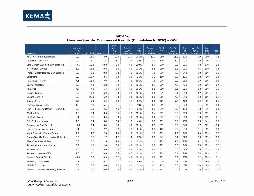
Xcel Energy Minnesota April 20, 2012 DSM Market Potential Assessment
5-27
Table 5-6 Measure-Specific Commercial Results (Cumulative to 2020) – GWh
Measure
Average TRC Ratio Technical Economic
Econ Net of Nat
OCC
Ach @ 100%
Incentives
% of Net
Econ
Ach @ 75%
Incentives
% of Net
Econ
Ach @ 50%
Incentives
% of Net
Econ
Ach @ BAU
Incentives
% of Net
Econ Nat Occ
VSD - Chiller Pumps/Towers 2.2 13.0 13.0 12.6 12.7 101% 12.3 98% 11.2 89% 9.9 79% 0.4
HE Refrig Fan Motors 9.3 11.6 11.6 11.5 2.6 23% 1.5 13% 1.0 9% 0.9 8% 0.1
Data Center State of the Art practices 10.5 10.8 10.8 9.0 9.0 100% 8.7 97% 8.3 93% 7.8 87% 1.9
Air Handler Tuneups 1.3 15.2 9.3 9.0 9.0 101% 8.8 98% 8.3 93% 7.5 83% 0.4
Freezer-Cooler Replacement Gaskets 9.2 9.3 9.3 7.8 7.9 101% 7.6 97% 7.3 94% 6.9 89% 1.5
Delamping 0.8 110.7 8.4 8.4 2.6 31% 1.3 16% 0.9 10% 0.8 9% 0.0
Heat Recovery Unit 4.1 11.0 7.9 7.3 7.3 101% 7.1 97% 6.6 91% 6.0 82% 0.6
Ceiling Insulation 2.7 7.3 6.8 6.2 6.2 101% 5.7 93% 4.8 77% 3.9 63% 0.7
Heat Trap 4.7 7.2 6.4 5.9 6.0 101% 5.8 98% 5.6 95% 5.3 90% 0.5
Cooling Tuneup 0.7 19.3 5.9 5.8 5.8 101% 5.6 97% 5.1 88% 4.2 73% 0.1
Cooling Controls 0.7 22.9 5.9 5.8 5.8 101% 5.5 96% 4.9 84% 3.9 68% 0.1
Efficient Fryer 5.7 5.6 5.5 5.4 3.7 69% 3.1 58% 2.7 49% 2.4 45% 0.1
Tankless Water Heater 1.3 7.6 5.1 5.1 0.7 13% 0.3 6% 0.2 4% 0.1 3% 0.0
High Perf Building Design - Near ZNE 0.9 15.0 4.5 4.5 2.4 54% 0.9 21% 0.5 12% 0.3 7% 0.0
Window Film 1.2 12.4 3.6 3.5 3.5 101% 3.4 98% 3.2 93% 2.9 85% 0.1
HE Chiller Motors 2.1 3.5 3.4 3.3 3.3 101% 3.2 97% 2.9 86% 2.8 83% 0.1
Cold Cathode Lamps 1.3 3.4 3.4 3.4 1.5 46% 0.9 25% 0.5 16% 0.5 14% 0.0
Demand Hot Gas Defrost 16.3 3.4 3.4 3.0 3.0 101% 2.9 98% 2.8 94% 2.7 90% 0.4
High Efficiency Water Heater 2.1 2.5 2.2 2.2 0.5 21% 0.3 12% 0.2 8% 0.1 6% 0.0
Night Covers for Display Cases 2.2 4.7 2.0 1.8 1.8 101% 1.7 98% 1.7 94% 1.6 90% 0.2
Energy Star Hot Food Holding Cabinets 0.5 6.5 1.7 1.7 1.2 67% 0.6 34% 0.4 22% 0.3 18% 0.0
Fiber Optic Case Lighting 0.3 15.7 1.5 1.4 1.4 101% 1.4 98% 1.3 90% 1.1 79% 0.0
Refrigeration Commissioning 6.2 1.6 1.0 0.9 0.9 101% 0.8 97% 0.8 94% 0.8 89% 0.2
Refrig Controls 2.5 0.6 0.6 0.6 0.6 101% 0.6 98% 0.5 94% 0.5 87% 0.0
Refrig Compressor VSD 2.8 7.1 0.6 0.5 0.5 101% 0.5 97% 0.4 94% 0.4 89% 0.1
Demand Defrost Electric 44.6 0.3 0.3 0.2 0.2 101% 0.2 97% 0.2 93% 0.2 88% 0.1
HE Refrig Compressor 6.7 0.1 0.1 0.1 0.1 69% 0.1 60% 0.1 52% 0.1 49% 0.0
HE PTAC Cooling 0.5 10.2 0.0 0.0 0.0 32% 0.0 13% 0.0 8% 0.0 9% 0.0
Demand controlled circulating systems 0.2 2.0 0.0 0.0 0.0 101% 0.0 96% 0.0 83% 0.0 69% 0.0

Xcel Energy Minnesota April 20, 2012 DSM Market Potential Assessment
5-28
Table 5-6 Measure-Specific Commercial Results (Cumulative to 2020) – GWh
Measure
Average TRC Ratio Technical Economic
Econ Net of Nat
OCC
Ach @ 100%
Incentives
% of Net
Econ
Ach @ 75%
Incentives
% of Net
Econ
Ach @ 50%
Incentives
% of Net
Econ
Ach @ BAU
Incentives
% of Net
Econ Nat Occ
Economizer 0.7 94.1 0.0 0.0 0.0 0% 0.0 0% 0.0 0% 0.0 0% 0.0
Duct/Pipe Insulation 0.1 10.5 0.0 0.0 0.0 0% 0.0 0% 0.0 0% 0.0 0% 0.0
Geothermal Heat Pump 0.3 11.3 0.0 0.0 0.0 0% 0.0 0% 0.0 0% 0.0 0% 0.0
Energy Recovery Vent 0.3 8.5 0.0 0.0 0.0 0% 0.0 0% 0.0 0% 0.0 0% 0.0
High R-Value Refrig Glass Doors 0.1 0.7 0.0 0.0 0.0 0% 0.0 0% 0.0 0% 0.0 0% 0.0
Multiplex Refrig Compressor System 0.5 0.7 0.0 0.0 0.0 0% 0.0 0% 0.0 0% 0.0 0% 0.0
Refrig Strip Curtains 0.0 0.4 0.0 0.0 0.0 0% 0.0 0% 0.0 0% 0.0 0% 0.0
LED Refrig Case Lighting 0.3 1.0 0.0 0.0 0.0 0% 0.0 0% 0.0 0% 0.0 0% 0.0
Hot Water Pipe Insulation 0.5 0.8 0.0 0.0 0.0 0% 0.0 0% 0.0 0% 0.0 0% 0.0
Vending Misers 0.4 3.4 0.0 0.0 0.0 0% 0.0 0% 0.0 0% 0.0 0% 0.0
Convection Oven 0.2 1.3 0.0 0.0 0.0 0% 0.0 0% 0.0 0% 0.0 0% 0.0
Note: TRC ratios are averages across multiple market segments. In some cases, the average TRC ratio may be below 1.0, but the measure is cost effective for some market segments, and thus, economic savings can be positive. In some cases achievable potential at the 100% incentives scenario exceeds net economic potential by a small amount; this is due to rounding error.

Xcel Energy Minnesota April 20, 2012 DSM Market Potential Assessment
5-29
5.2.1.3 Industrial Sector
Figure 5-35 shows cumulative net achievable program savings by industrial program scenario. By 2020, energy savings reach 725 GWh under the BAU scenario, 808 GWh under the 50-percent incentive scenario, 888 GWh under the 75-percent incentive scenario, and 1,007 GWh under the 100-percent incentive scenario.
Figure 5-35 Achievable Energy Savings: Industrial Sector
0
200
400
600
800
1,000
1,200
2011 2012 2013 2014 2015 2016 2017 2018 2019 2020
Cum
ulat
ive
Annu
al S
avin
gs -
GW
h
Nat Occ
100% Incent
75% Incent
50% Incent
BAU Incent
Figure 5-36 and Figure 5-37 show the end-use distribution of energy and peak-demand savings in the industrial sector. Similar to technical and economic potential, cross-cutting motor end uses (compressed air, fans, and pumps) account for the majority of savings. The fan end use shows a large increase between the 75-percent and 100-percent incentive scenarios due to fan control measures being offered at no incremental cost.

Xcel Energy Minnesota April 20, 2012 DSM Market Potential Assessment
5-30
Figure 5-36 Industrial Energy-Savings Potential
by End-Use (2020)
Figure 5-37 Industrial Peak-Savings Potential
by End-Use (2020)
208
269
179
128
45
75
18
11
72
195
208
166
110
40
72
16
11
71
183
176
155
98
36
67
14
10
68
170
150
141
86
32
59
12
9
66
0 100 200 300
Compressed Air
Fans
Pumping
Drives
Process Heating
Refrigeration
Other Process
Cooling
Lighting
Cumulative Annual Savings by 2020 - GWh
100% Incent75% Incent50% IncentBAU Incent
23.7
25.2
17.4
15.8
5.8
9.0
2.3
1.0
10.5
22.0
18.5
15.9
13.5
5.1
8.6
2.0
0.9
10.2
20.6
15.1
14.7
12.0
4.6
8.0
1.8
0.9
9.9
19.0
12.5
13.3
10.5
4.0
7.0
1.6
0.8
9.5
0 10 20 3
Compressed Air
Fans
Pumping
Drives
Process Heating
Refrigeration
Other Process
Cooling
Lighting
Cumulative Peak Savings by 2020 - MW0
100% Incent75% Incent50% IncentBAU Incent
Figure 5-38 and Figure 5-39 show industrial savings by industry type. Food processing and petroleum are the leading sources of potential. Similar to the commercial sector, savings potentials start our fairly high for the BAU scenario and increase gradually with higher program-effort scenarios.

Xcel Energy Minnesota April 20, 2012 DSM Market Potential Assessment
5-31
Figure 5-38 Industrial Energy-Savings Potential
by End-Use (2020)
Figure 5-39 Industrial Peak-Savings Potential
by End-Use (2020)
215
3
21
54
55
72
168
75
39
36
45
80
59
20
49
18
192
3
19
44
49
63
144
61
33
31
42
75
54
19
45
15
174
3
18
38
45
57
131
53
29
28
39
70
50
17
42
13
154
3
16
34
41
51
118
46
26
25
35
64
46
16
39
12
0 50 100 150 200 250
Food
Textiles-Apparel
Lumber-Furniture
Paper
Printing
Chemicals
Petroleum
Rubber-Plastics
Stone-Clay-Glass
Prim Metals
Fab Metals
Ind Mach
Electronics
Transp Equip
Misc Ind
Water/WW
Cumulative Annual Savings by 2020 - GWh
100% Incent
75% Incent
50% Incent
BAU Incent
22.1
1.2
2.7
3.7
6.2
7.0
15.7
9.1
3.4
4.3
5.3
14.8
6.3
2.3
4.7
1.6
19.5
1.1
2.5
3.0
5.5
6.0
13.2
7.3
2.7
3.7
4.8
13.7
5.8
2.1
4.3
1.3
17.6
1.0
2.3
2.6
5.1
5.4
11.8
6.2
2.4
3.4
4.5
12.8
5.4
2.0
4.0
1.1
15.5
1.0
2.0
2.3
4.5
4.8
10.5
5.4
2.1
3.0
4.1
11.8
4.9
1.8
3.6
1.0
0.0 10.0 20.0 30.0
Food
Textiles-Apparel
Lumber-Furniture
Paper
Printing
Chemicals
Petroleum
Rubber-Plastics
Stone-Clay-Glass
Prim Metals
Fab Metals
Ind Mach
Electronics
Transp Equip
Misc Ind
Water/WW
Cumulative PeakSavings by 2020 - MW
100% Incent
75% Incent
50% Incent
BAU Incent

Xcel Energy Minnesota April 20, 2012 DSM Market Potential Assessment
5-32
Table 5-7 lists the various potentials for industrial measures. There are a large number of industrial measures that contribute to industrial savings potential. Limited penetration of some industrial measures is, in part, due equipment turnover cycles that limit energy-efficiency opportunities.
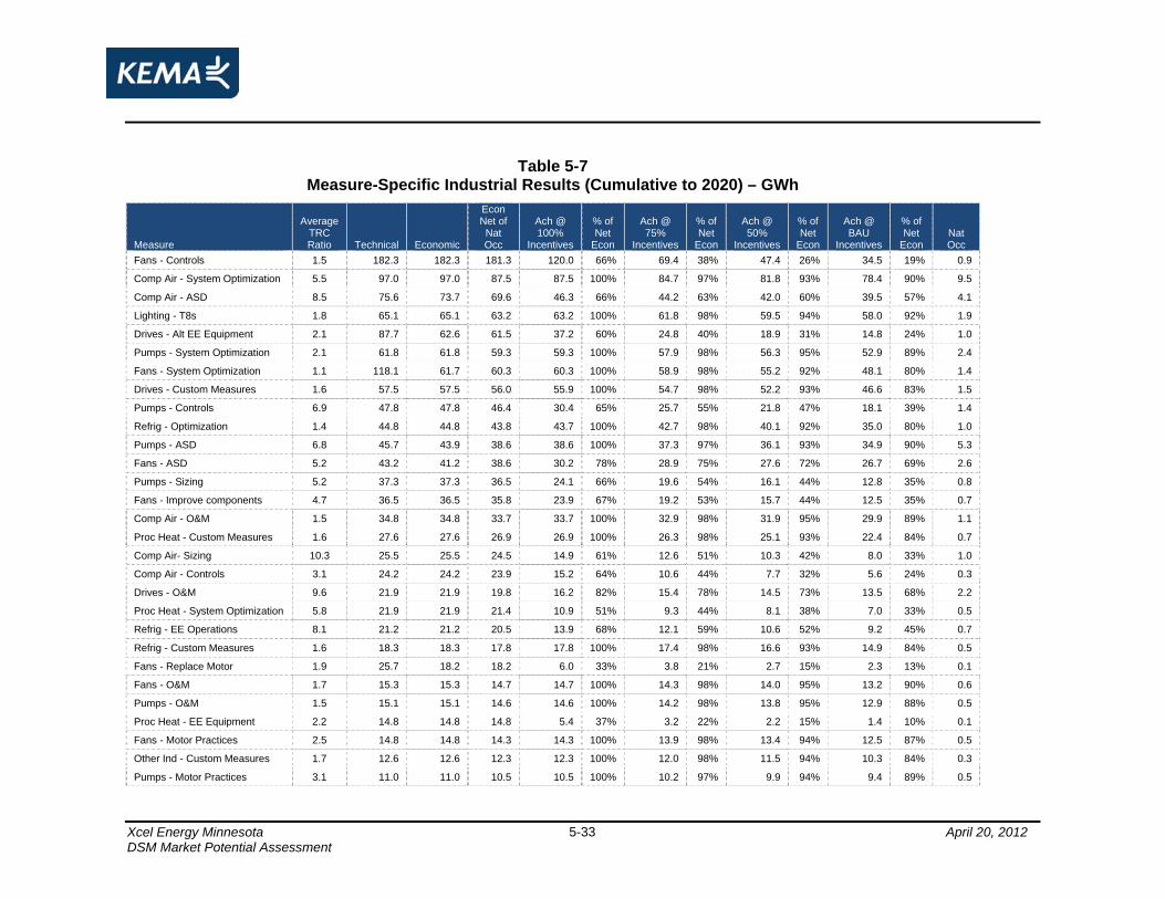
Xcel Energy Minnesota April 20, 2012 DSM Market Potential Assessment
5-33
Table 5-7 Measure-Specific Industrial Results (Cumulative to 2020) – GWh
Measure
Average TRC Ratio Technical Economic
Econ Net of Nat Occ
Ach @ 100%
Incentives
% of Net
Econ
Ach @ 75%
Incentives
% of Net
Econ
Ach @ 50%
Incentives
% of Net
Econ
Ach @ BAU
Incentives
% of Net
Econ Nat Occ
Fans - Controls 1.5 182.3 182.3 181.3 120.0 66% 69.4 38% 47.4 26% 34.5 19% 0.9
Comp Air - System Optimization 5.5 97.0 97.0 87.5 87.5 100% 84.7 97% 81.8 93% 78.4 90% 9.5
Comp Air - ASD 8.5 75.6 73.7 69.6 46.3 66% 44.2 63% 42.0 60% 39.5 57% 4.1
Lighting - T8s 1.8 65.1 65.1 63.2 63.2 100% 61.8 98% 59.5 94% 58.0 92% 1.9
Drives - Alt EE Equipment 2.1 87.7 62.6 61.5 37.2 60% 24.8 40% 18.9 31% 14.8 24% 1.0
Pumps - System Optimization 2.1 61.8 61.8 59.3 59.3 100% 57.9 98% 56.3 95% 52.9 89% 2.4
Fans - System Optimization 1.1 118.1 61.7 60.3 60.3 100% 58.9 98% 55.2 92% 48.1 80% 1.4
Drives - Custom Measures 1.6 57.5 57.5 56.0 55.9 100% 54.7 98% 52.2 93% 46.6 83% 1.5
Pumps - Controls 6.9 47.8 47.8 46.4 30.4 65% 25.7 55% 21.8 47% 18.1 39% 1.4
Refrig - Optimization 1.4 44.8 44.8 43.8 43.7 100% 42.7 98% 40.1 92% 35.0 80% 1.0
Pumps - ASD 6.8 45.7 43.9 38.6 38.6 100% 37.3 97% 36.1 93% 34.9 90% 5.3
Fans - ASD 5.2 43.2 41.2 38.6 30.2 78% 28.9 75% 27.6 72% 26.7 69% 2.6
Pumps - Sizing 5.2 37.3 37.3 36.5 24.1 66% 19.6 54% 16.1 44% 12.8 35% 0.8
Fans - Improve components 4.7 36.5 36.5 35.8 23.9 67% 19.2 53% 15.7 44% 12.5 35% 0.7
Comp Air - O&M 1.5 34.8 34.8 33.7 33.7 100% 32.9 98% 31.9 95% 29.9 89% 1.1
Proc Heat - Custom Measures 1.6 27.6 27.6 26.9 26.9 100% 26.3 98% 25.1 93% 22.4 84% 0.7
Comp Air- Sizing 10.3 25.5 25.5 24.5 14.9 61% 12.6 51% 10.3 42% 8.0 33% 1.0
Comp Air - Controls 3.1 24.2 24.2 23.9 15.2 64% 10.6 44% 7.7 32% 5.6 24% 0.3
Drives - O&M 9.6 21.9 21.9 19.8 16.2 82% 15.4 78% 14.5 73% 13.5 68% 2.2
Proc Heat - System Optimization 5.8 21.9 21.9 21.4 10.9 51% 9.3 44% 8.1 38% 7.0 33% 0.5
Refrig - EE Operations 8.1 21.2 21.2 20.5 13.9 68% 12.1 59% 10.6 52% 9.2 45% 0.7
Refrig - Custom Measures 1.6 18.3 18.3 17.8 17.8 100% 17.4 98% 16.6 93% 14.9 84% 0.5
Fans - Replace Motor 1.9 25.7 18.2 18.2 6.0 33% 3.8 21% 2.7 15% 2.3 13% 0.1
Fans - O&M 1.7 15.3 15.3 14.7 14.7 100% 14.3 98% 14.0 95% 13.2 90% 0.6
Pumps - O&M 1.5 15.1 15.1 14.6 14.6 100% 14.2 98% 13.8 95% 12.9 88% 0.5
Proc Heat - EE Equipment 2.2 14.8 14.8 14.8 5.4 37% 3.2 22% 2.2 15% 1.4 10% 0.1
Fans - Motor Practices 2.5 14.8 14.8 14.3 14.3 100% 13.9 98% 13.4 94% 12.5 87% 0.5
Other Ind - Custom Measures 1.7 12.6 12.6 12.3 12.3 100% 12.0 98% 11.5 94% 10.3 84% 0.3
Pumps - Motor Practices 3.1 11.0 11.0 10.5 10.5 100% 10.2 97% 9.9 94% 9.4 89% 0.5

Xcel Energy Minnesota April 20, 2012 DSM Market Potential Assessment
5-34
Table 5-7 Measure-Specific Industrial Results (Cumulative to 2020) – GWh
Measure
Average TRC Ratio Technical Economic
Econ Net of Nat Occ
Ach @ 100%
Incentives
% of Net
Econ
Ach @ 75%
Incentives
% of Net
Econ
Ach @ 50%
Incentives
% of Net
Econ
Ach @ BAU
Incentives
% of Net
Econ Nat Occ
Other Ind - EE Equipment 3.8 9.2 9.2 9.1 4.0 44% 2.9 31% 2.0 22% 1.4 15% 0.1
Drives - Controls 1.8 10.1 8.9 8.8 5.5 63% 3.4 39% 2.4 27% 1.7 19% 0.1
Comp Air - Motor Practices 2.7 8.7 8.7 8.4 8.4 100% 8.2 97% 7.8 94% 7.4 88% 0.3
Lighting - Controls 1.7 8.5 8.5 8.2 8.2 100% 8.0 98% 7.7 94% 7.1 86% 0.2
Drives - System Optimization 3.2 8.5 8.5 8.0 8.0 100% 7.8 97% 7.5 94% 6.9 87% 0.5
Drives - EE Equipment 2.3 10.2 7.9 7.8 5.2 66% 3.7 48% 2.8 36% 2.3 29% 0.1
Cooling - Controls 6.4 7.5 7.0 5.8 5.8 100% 5.5 96% 5.3 92% 5.0 86% 1.2
Cooling - Window Film 1.6 5.4 5.1 5.0 5.0 100% 4.9 98% 4.7 94% 4.2 85% 0.1
Pumps - Replace Motor 1.2 13.0 4.8 4.7 1.5 33% 0.9 20% 0.6 14% 0.5 11% 0.0
Comp Air - Replace Motor 1.4 8.4 4.4 4.3 1.4 31% 0.8 18% 0.5 12% 0.4 8% 0.0
Other Ind - Controls 1.5 3.2 3.2 3.2 2.1 65% 1.2 38% 0.8 26% 0.6 17% 0.0
Proc Heat - Controls 2.2 2.1 2.1 2.1 0.9 44% 0.6 27% 0.4 19% 0.3 14% 0.0
Proc Heat - Alt EE Equipment 3.9 2.1 2.1 2.0 1.1 54% 0.8 39% 0.6 31% 0.5 24% 0.0
Cooling - HE Chiller 3.2 1.2 1.2 1.2 0.4 31% 0.2 21% 0.2 14% 0.1 13% 0.0
Lighting - CFLs 1.4 1.0 0.9 0.9 0.9 100% 0.9 98% 0.9 94% 0.8 92% 0.0
Comp Air - Power recovery 1.1 0.8 0.8 0.8 0.8 100% 0.8 97% 0.8 91% 0.6 78% 0.0
Cooling - EE DX 0.8 10.6 0.1 0.1 0.0 33% 0.0 11% 0.0 6% 0.0 6% 0.0
Other EE Measures 2.2 0.0 0.0 0.0 0.0 74% 0.0 53% 0.0 39% 0.0 28% 0.0
Cooling - Equipment Tuneup 0.2 7.1 0.0 0.0 0.0 100% 0.0 95% 0.0 82% 0.0 81% 0.0
Cooling - Cool Roof 0.4 5.8 0.0 0.0 0.0 0% 0.0 0% 0.0 0% 0.0 0% 0.0
Cooling - VSD Pumps 0.3 0.3 0.0 0.0 0.0 0% 0.0 0% 0.0 0% 0.0 0% 0.0
Lighting - Metal Halide 0.2 82.9 0.0 0.0 0.0 0% 0.0 0% 0.0 0% 0.0 0% 0.0
Note: TRC ratios are averages across multiple market segments. In some cases, the average TRC ratio may be below 1.0, but the measure is cost effective for some market segments, and thus, economic savings can be positive.

Xcel Energy Minnesota April 20, 2012 DSM Market Potential Assessment
5-35
5.3 Behavioral Conservation and Emerging Technologies In addition to the base energy-efficiency potential forecast described above, we also investigated the effects of behavioral conservation and emerging technologies. The impacts of these components are much more uncertain than the impacts of the more standard, commercially available measures that are included in the base analysis, and this is why they receive separate treatment.
5.3.1 Behavioral Conservation
Residential behavioral-conservation programs have shown some promise in motivating customers to use less energy. However, factors such as persistence and the expected amount of energy savings have not been tested over a significant period of time or across a wide range of customers. Programs can include both direct and indirect feedback methods. The direct methods involve in-home installation of feedback devices that monitor energy usage and provide the customer with real time information on consumption. Indirect methods involve periodic reporting to customers, providing information such as: comparisons to neighbors’ energy usage, assessment of energy usage by appliance, tips for reducing energy consumption, and information about programs that can be utilized to help in the energy reduction effort.
For this analysis, we focused on indirect feedback methods since these are experiencing wider adoption by utilities across the U.S. Also, there is probably a lot of overlap in the impacts of these two methods, but this overlap is not well understood, so we present potential impacts from the indirect approach, with the understanding that these impacts can serve as a proxy for savings from both types of behavior-motivation methods.
We assumed that the indirect measures would save about two percent of household energy consumption at a cost of about $7 per customer per year (after netting out the portion of program costs that could be allocated to natural gas savings). These measures could be offered to the entire residential population, or targeted to strategic subsets of the population. Direct methods could save somewhat more energy, about five percent per year, at an equipment cost of about $140 per customer, with a measure life of four years. These direct methods could be applied to between five and ten percent of the residential population, and are sometimes considered most effective for customer groups that are already very interested in energy usage and energy reduction efforts. Both direct and indirect measure parameters noted above are
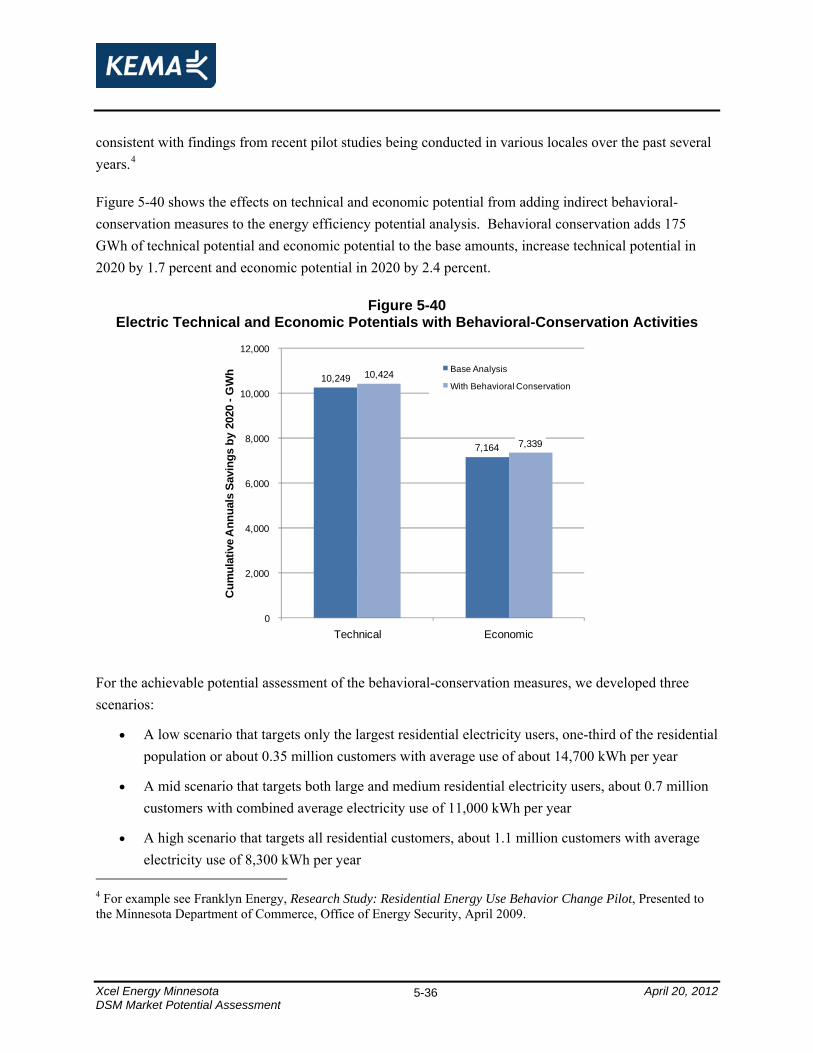
Xcel Energy Minnesota April 20, 2012 DSM Market Potential Assessment
5-36
consistent with findings from recent pilot studies being conducted in various locales over the past several years.4
Figure 5-40 shows the effects on technical and economic potential from adding indirect behavioral-conservation measures to the energy efficiency potential analysis. Behavioral conservation adds 175 GWh of technical potential and economic potential to the base amounts, increase technical potential in 2020 by 1.7 percent and economic potential in 2020 by 2.4 percent.
Figure 5-40 Electric Technical and Economic Potentials with Behavioral-Conservation Activities
10,249
7,164
10,424
7,339
0
2,000
4,000
6,000
8,000
10,000
12,000
Technical Economic
Cum
ulat
ive
Ann
uals
Sav
ings
by
2020
-G
Wh Base Analysis
With Behavioral Conservation
For the achievable potential assessment of the behavioral-conservation measures, we developed three scenarios:
• A low scenario that targets only the largest residential electricity users, one-third of the residential population or about 0.35 million customers with average use of about 14,700 kWh per year
• A mid scenario that targets both large and medium residential electricity users, about 0.7 million customers with combined average electricity use of 11,000 kWh per year
• A high scenario that targets all residential customers, about 1.1 million customers with average electricity use of 8,300 kWh per year
4 For example see Franklyn Energy, Research Study: Residential Energy Use Behavior Change Pilot, Presented to the Minnesota Department of Commerce, Office of Energy Security, April 2009.

Xcel Energy Minnesota April 20, 2012 DSM Market Potential Assessment
5-37
In each case, program efforts were ramped up over a three-year period. Table 5-8 summarizes the results of the analysis over the 2011-2020 time period. As shown, behavioral-conservation potentials—if the assumptions outlined above hold up—could save between 102 and 174 GWh per year, with annual program costs ranging between $22 million and $67 million dollars over a 10-year period, depending on how many customers are targeted for the indirect interventions. (It is also possible that Xcel Energy could reduce program costs by better targeting customers, so these estimates are probably an upper-bound of program costs.) All scenarios have TRC ratios that are greater than 1.0, the cutoff for cost-effectiveness. The scenarios that target the larger users show the highest TRC ratios because energy savings per customer are assumed to be higher, while program costs are the same as for lower-use customers.
Table 5-8 Achievable Potentials for Electric Behavioral Conservation
Scenario: Low: Medium: High:
Result Large Users Only Lrg-Med Users All Customers
Total Market Energy Savings - GWh 102.03 152.27 174.67 Total Market Peak Demand Savings - MW 27.64 41.25 47.31 Program Energy Savings – Net GWh 102.03 152.27 174.67 Program Peak Demand Savings – Net MW 27.64 41.25 47.31
Program Costs - Real, $ Million Administration $0.20 $0.35 $0.51 Marketing $21.85 $43.70 $66.31 Incentives $0.00 $0.00 $0.00 Total $22.05 $44.05 $66.81
PV Avoided Costs $53.86 $80.39 $92.21 PV Annual Program Costs (Adm/Mkt) $17.14 $34.24 $51.94 PV Net Measure Costs $0.00 $0.00 $0.00 Net Benefits $36.72 $46.15 $40.27 TRC Ratio 3.1 2.3 1.8
PV (present value) of benefits and costs is calculated for 2011-2020 program years using a nominal discount rate = 7.4 percent, and an assumed inflation rate = 1.9 percent; GWh and MW savings are cumulative through 2020.
5.3.2 Emerging Technologies
The ultimate impacts and timing of emerging technologies are very uncertain due to both technological and market barriers. Despite these uncertainties associated with particular technologies, we know that energy-efficiency measures will continue to evolve, and emerging technologies will play a significant role in future program years.

Xcel Energy Minnesota April 20, 2012 DSM Market Potential Assessment
5-38
In order to address the possible effects of emerging energy-efficiency measures, KEMA developed a modeling approach that combines a bottom-up method for estimating technical and economic potential of emerging technologies with a technology diffusion analysis to estimate possible market penetration for these technologies over time.
The following steps were utilized in the analysis:
Identification of technologies and applications to be used in the study: A list of 41 technologies that are expected to be commercially available by 2014 were taken from a U.S. Department of Energy publication5 and augmented with 4 additional technologies requested by Xcel Energy to provide a total of 45 technologies to be investigated in the study.
Segment the selected technologies by market and end use: Each measure was categorized by its end use and the market segment it applied to. Baseline measures and energy use were determined from this categorization, consistent with the base energy efficiency potential analysis.
Populate the model: We researched publications and contacted research groups and manufacturers to get an understanding of product commercialization dates, pricing structures, and estimated savings. For technologies already in the market, pricing, estimated useful life, expected payback period, power draw, and likely application were gathered from manufacturers’ catalogues. For technologies still in development, KEMA research similar competitor products and projected necessary model inputs based on trends and patterns. At this point some products were removed from the research list because their introduction to the market was deemed not feasible given current R&D and funding efforts. Fourteen measures (4 HVAC, 1 Motor, and 9 Lighting) were included in the final model, all directed toward the commercial sector.
Estimate market potential: Technical potential was calculated is a similar fashion to the base energy efficiency potential analysis. Economic potential was also calculated using the same benefit/cost screening as the base analysis.
Estimate market penetration: The market penetration calculation uses a logit functional form (an S-shaped curve), based on the traditional BASS technology diffusion curve, to trace the adoption path of the technologies. In a variation on the BASS curve, the functional form used in this study uses the first year of practical market availability and the number of years to capture 50 percent of the technical potential as input parameters instead of the traditional BASS coefficients of innovation and imitation. For emerging technologies, this provides a more intuitive approach to understanding the process and outputs of the forecast. 5 Buildings R&D Breakthroughs: Technologies and Products Supported by the Building Technologies Program, U.S. Department of Energy’s Office of Energy Efficiency and Renewable Energy, June, 22, 2011.

Xcel Energy Minnesota April 20, 2012 DSM Market Potential Assessment
5-39
Simulation: to summarize the possible energy savings and adoption paths into the future, we varied one key modeling parameter, the incremental cost of the emerging technology, and generated three forecast scenarios. In the model, the incremental costs influence the number of years to capture 50 percent of the market. The working assumption was that emerging technology prices will come down over time, but as payback increased, we extended the number of years to capture 50 percent of the market because greater improvements or efficiencies need to be made to make the technologies more competitive. We adjusted the initial year of earnest sales in a similar fashion. Table 5-9 lists the diffusion parameters used in the analysis:
Table 5-9 Emerging Technology Diffusion Parameters
Simple payback Years to capture 50% of market
Sales start year (earnest)
=< 2.0 years 7 year + 0
=< 2.5 years 10 ---
=< 3.0 years 12 year + 3
> 3.0 years 15 ---
=< 5.0 years 15 year + 4
5.3.2.1 Results
The following 14 technologies were included in the final analysis:
1. HVAC: Liquid Desiccant Air Conditioner (2.5 hp)
2. HVAC: Liquid Desiccant Air Conditioner (5hp)
3. HVAC: Ammonia Absorption Technologies for HVAC systems
4. HVAC: Hypak: A high efficiency rooftop packaged HVAC system
5. Lighting: LED High-Bay fixtures
6. Lighting: LED replacement fixture for linear fluorescent area lighting
7. Lighting: LED replacement for linear fluorescent lamps in existing fixtures
8. Lighting: Electro-Ceramescent, low power Light-Emitting Device
9. Lighting: 100 Lumen/ Watt warm white LED (lamp only)
10. Lighting: 100 Lumen/ Watt warm white LED (lamp and fixture)
11. Lighting: HE solid-state down light luminaires w/ novel cooling
12. Lighting: Efficient LED System-in-Module for general lighting
13. Lighting: Kilo-Lumen SSL exceeding 100 lumens per Watt

Xcel Energy Minnesota April 20, 2012 DSM Market Potential Assessment
5-40
14. Motors: Nova Torque highly efficient electric motor
The three simulations run for the analysis are described here and summarized in Table 5-10 and Figure 5-41 through Figure 5-43. (Note that the emerging technology savings potential estimates do not factor in overlap with the base energy efficiency potential results. A subsequent analysis was conducted to determine that approximately half of the emerging technology potentials could be incremental to measures already addressed in the base analysis. The incremental results are presented in Table 5-11 below.)
• Baseline: incremental costs at 100 percent (baseline) and potential of success at 100 percent.
• Scenario 1: incremental costs at 75 percent of baseline and potential of success at 100 percent.
• Scenario 2: incremental costs at 25 percent of baseline and potential of success at 100 percent.
Table 5-10 Summary of Emerging Technology Simulations
Scenario Technical Potential Economic Potential Capture Capture MW GWh (20 Yr) GWh (10 Yr) (20 Yr)
Baseline 1,190 4,137 840 3,143 38% 76%
Scenario 1 - little change 1,190 4,137 870 3,349 41% 81%
Scenario 2 - competition 1,190 4,137 950 3,601 47% 87%
Note: Potentials reflect savings over base technologies and are not adjusted for overlap with base energy efficiency results.

Xcel Energy Minnesota April 20, 2012 DSM Market Potential Assessment
5-41
Figure 5-41 Emerging Technology: Baseline Adoption Path
0
250
500
750
1,000
1,250
1,500
1,750
2,000
2,250
2011 2013 2015 2017 2019 2021 2023 2025 2027 2029
Cum
ulat
ive
Annu
al S
avin
gs -
GW
hLightingHVACMotors
Figure 5-42 Emerging Technology: Scenario 1 (Little Change) Path - 25% Cost Reduction
-
250
500
750
1,000
1,250
1,500
1,750
2,000
2,250
2011 2013 2015 2017 2019 2021 2023 2025 2027 2029
Cum
ulat
ive
Annu
al S
avin
gs -
GW
h
LightingHVACMotors

Xcel Energy Minnesota April 20, 2012 DSM Market Potential Assessment
5-42
Figure 5-43 Emerging Technology: Scenario 2 (Competition) Path – 75% Cost Reduction
0
250
500
750
1,000
1,250
1,500
1,750
2,000
2,250
2011 2013 2015 2017 2019 2021 2023 2025 2027 2029
Cum
ulat
ive
Annu
al S
avin
gs -
GW
hLightingHVACMotors
The emerging technology analysis focused on measure saving in relation to base technology, but this analysis double counts with some savings already contained in base energy efficiency potential results discuss in prior subsections. A review of the emerging technology savings in relation to competing energy efficiency technologies revealed that just under 50 percent of the emerging technology savings presented above could be incremental to the base energy efficiency analysis. Incremental savings estimates are presented in the last two columns of Table 5-11.
Table 5-11 Incremental Emerging Technology Savings Potentials
Scenario Total Economic Potential Incremental Economic Potential MW GWh MW GWh
Baseline 840 3,143 395 1,477
Scenario 1 - Little Change 870 3,349 409 1,574
Scenario 2 - Competition 950 3,601 447 1,692
5.3.2.2 Discussion of Results
The availability, timing and ultimate adoption of emerging technologies is inherently uncertain. We know that many of these technologies will improve and evolve. We also know that most incumbent technologies will not give away their market share quietly. These technologies also will innovate to keep their current pricing and applicability advantages.

Xcel Energy Minnesota April 20, 2012 DSM Market Potential Assessment
5-43
As Figure 5-41 to Figure 5-43 show, the HVAC measures under review showlarge penetration across all three scenarios. The measure contributing most to HVAC potential promises very good cost savings over existing technologies and should find fairly good market acceptance. The Scenario 1 adoption path is not very different from the Baseline path, indication that further price reductions (either by the manufacturer or through utility incentives) will not do much to push the market. Only under larger cost reductions (Scenario 2) does the penetration increase in a significant way.
For the lighting and motor measures, large cost reductions or incentives may be necessary to move the market substantially beyond the baseline path, as illustrated by the Baseline and Scenario 1 figure not showing much difference and only the Scenario 2 with 75 percent cost reductions leading to a significant increase in penetration.
Overall, the emerging technologies may provide a significant boost to future energy efficiency portfolios, and market developments should be monitored. Depending on cost assumptions, the emerging technologies studied here could increase base energy efficiency potential of 7,164 GWh by over 20 percent.
As these emerging technologies become market-ready, the use of program incentives may be useful in acceleration measure uptake, but it is likely that, at least initially, incentives would need to cover a large portion of the incremental measure cost.

Xcel Energy Minnesota April 20, 2012 DSM Market Potential Assessment
6-1
6. Demand Response Potential Results
KEMA estimated the potential of demand response (DR) programs by customizing inputs to the model developed to support the Federal Energy Regulatory Commission’s 2009 National Assessment of Demand Response Potential6.KEMA customized inputs to the National Assessment of Demand Response (NADR) model to represent the Xcel Energy Minnesota service territory by using information on Xcel Energy data, forecasts, and current program accomplishments.
The NADR model uses a bottom-up approach to estimate DR resources. The model estimates impacts for four customer segments (residential and small, medium, and large nonresidential segments) and five DR program categories (direct load control, interruptible rates, dynamic pricing with enabling technologies, dynamic pricing without enabling technologies, and other DR programs such as demand bidding). Estimates are developed for four different scenarios:
• Business-as-usual (BAU): current programs and tariffs are held constant;.
• Expanded BAU (EBAU): BAU program participation rates are increased to equal the 75th percentile of ranked participation rates of similar programs across the U.S.
• Achievable Participation (AP): further assumes advanced metering infrastructure (AMI) is universally deployed, and dynamic pricing is the opt-out default tariff.
• Full Participation (FP): similar to the AP scenario, except that dynamic pricing and the acceptance of enabling technology is mandatory. This scenario quantifies the maximum cost-effective DR potential, absent any regulatory and market barriers.
For the Xcel Energy Minnesota analysis, we recalibrated the NADR model’s default Minnesota parameters to reflect Xcel Energy customer characteristics and adjusted the BAU scenario to reflect Xcel Energy’s current demand response program projections. For the other 3 scenarios (EBUA, AP, and FP), we applied the NADR model’s default assumptions to the Xcel Energy customer base to develop estimates of DR potential under expanded program offerings.
We note that the NADR model results should be qualified. As stated on page 18 of the 2009 NADR report:
“It is important to note that the results of the four scenarios are in fact estimates of potential, rather than projections of what is likely to occur. The numbers reported in this study should be interpreted
6 A National Assessment of Demand Response Potential, Staff Report, Federal Energy Regulatory Commission, prepared by The Brattle Group, Freeman, Sullivan & Co., and Global Energy Partners, LLC, June 2009.

Xcel Energy Minnesota April 20, 2012 DSM Market Potential Assessment
6-2
as the amount of demand response that could potentially be achieved under a variety of assumptions about the types of programs pursued, market acceptance of the programs, and the overall cost-effectiveness of the programs. This report does not advocate what programs/measures should be adopted/implemented by regulators; it only sets forth estimates should certain things occur.
As such, the estimates of potential in this report should not be interpreted as targets, goals, or requirements for individual states or utilities. However, by quantifying potential opportunities that exist in each state, these estimates can serve as a reference for understanding the various pathways for pursuing increased levels of demand response.
As with any model-based analysis in economics, the estimates in this Assessment are subject to a number of uncertainties, most of them arising from limitations in the data that are used to estimate the model parameters. Demand response studies performed with accurate utility data have had error ranges of up to ten percent of the estimated response per participating customer. In this analysis, the use of largely publicly-available, secondary data sources makes it likely that the error range for any particular estimate in each of the scenarios studied is larger, perhaps as high as twenty percent.”
There are a number of barriers to achieving the DR potentials developed in this study. These include:
• Constraints on the number of AMI installations which are required for critical peak pricing, with the understanding that there are many other factors with more significant costs and benefits that influence the decision to install AMI, beyond DR
• Regulatory barriers that include reluctance to adopt dramatically different pricing structures such as mandatory critical peak pricing and reluctance fund investments in AMI installations or in customer-side enabling technologies
• Technology barriers such as the limitations on cost-effective enabling technologies
• Customer barriers including: lack of awareness regarding DR, risk aversion to new technologies and pricing strategies, and perceived lack of ability to respond to DR events
These barriers may limit the ability to achieve the potentials developed in this analysis. In addition, the analysis does not address the need for DR. It just shows the peak savings reductions possible if a number of different DR strategies are implemented. Identifying the optimal amount of DR for Xcel Energy’s Minnesota service territory, taking into account DR resources and existing generation and T&D capacity, is outside the scope of this study.

Xcel Energy Minnesota April 20, 2012 DSM Market Potential Assessment
6-3
6.1 DR Potential Results Table 6-1 summarizes demand response potential estimates by scenario, DR mechanism and sector. Total DR potentials by 2020 increase from 941 MW in the BAU case to 1,209 MW in the Expanded BAU case to 1,444 MW in the Achievable Potential case to 1,552 MW in the Full Participation case. Potential reductions could increase from 12 percent of system peak in the BAU scenario up to 20 percent of system peak in the Full Participation scenario if these types of capacity reductions were needed on the Xcel Energy system.
Table 6-1 Demand Response Potential Results by Scenario, Mechanism, and Sector - 2020
Residential (MW)
Residential(% of
system)
Small C&I
(MW)
Small C&I
(% of system)
Med. C&I
(MW)
Med C&I
(% of system)
Large C&I
(MW)
Large C&I
(% of system)
Total (MW)
Total (% of
system)
BAU Pricing with Technology 0 0.0% 0 0.0% 0 0.0% 0 0.0% 0 0.0%
Pricing without Technology 0 0.0% 0 0.0% 0 0.0% 0 0.0% 0 0.0%
Automated/Direct Load Control 375 4.8% 12 0.2% 18 0.2% 33 0.4% 438 5.6%
Interruptible/Curtailable Tariffs 0 0.0% 0 0.0% 0 0.0% 503 6.5% 503 6.5%
Other DR Programs 0 0.0% 0 0.0% 0 0.0% 0 0.0% 0 0.0%
Total 375 4.8% 12 0.2% 18 0.2% 536 6.9% 941 12.1%
Expanded BAU Pricing with Technology 0 0.0% 0 0.0% 0 0.0% 0 0.0% 0 0.0%
Pricing without Technology 7 0.1% 0 0.0% 1 0.0% 3 0.0% 11 0.1%
Automated/Direct Load Control 375 4.8% 39 0.5% 18 0.2% 33 0.4% 465 6.0%
Interruptible/Curtailable Tariffs 0 0.0% 0 0.0% 10 0.1% 634 8.1% 643 8.3%
Other DR Programs 0 0.0% 0 0.0% 0 0.0% 90 1.2% 90 1.2%
Total 382 4.9% 39 0.5% 29 0.4% 758 9.7% 1,209 15.5%
Achievable Participation* Pricing with Technology 0 0.0% 0 0.0% 13 0.2% 0 0.0% 13 0.2%
Pricing without Technology 225 2.9% 1 0.0% 18 0.2% 60 0.8% 304 3.9%
Automated/Direct Load Control 375 4.8% 14 0.2% 18 0.2% 33 0.4% 440 5.6%
Interruptible/Curtailable Tariffs 0 0.0% 0 0.0% 10 0.1% 634 8.1% 643 8.3%
Other DR Programs 0 0.0% 0 0.0% 0 0.0% 44 0.6% 44 0.6%
Total 600 7.7% 15 0.2% 59 0.8% 770 9.9% 1,444 18.5%
Full Participation Pricing with Technology 0 0.0% 0 0.0% 37 0.5% 0 0.0% 37 0.5%
Pricing without Technology 301 3.9% 1 0.0% 19 0.2% 100 1.3% 422 5.4%
Automated/Direct Load Control 375 4.8% 12 0.2% 18 0.2% 33 0.4% 438 5.6%
Interruptible/Curtailable Tariffs 0 0.0% 0 0.0% 10 0.1% 634 8.1% 643 8.3%
Other DR Programs 0 0.0% 0 0.0% 0 0.0% 12 0.1% 12 0.1%
Total 676 8.7% 13 0.2% 85 1.1% 778 10.0% 1,552 19.9%
* Achievable Participation is the name given to a specific scenario in the FERC NADR study; these potentials are only achievable under the specific assumptions that define this scenario.
Figure 6-1 shows potential demand reductions in 2020 by DR scenario and sector. Most of the savings are concentrated in the residential and large C&I segments. As shown in the table above, most of the residential potential in the BAU and Expanded BAU scenarios comes from direct control activities, and the jump in
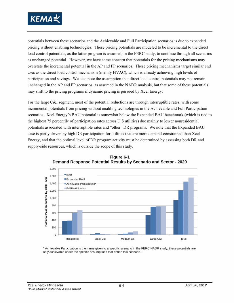
Xcel Energy Minnesota April 20, 2012 DSM Market Potential Assessment
6-4
potentials between these scenarios and the Achievable and Full Participation scenarios is due to expanded pricing without enabling technologies. These pricing potentials are modeled to be incremental to the direct load control potentials, as the latter program is assumed, in the FERC study, to continue through all scenarios as unchanged potential. However, we have some concern that potentials for the pricing mechanisms may overstate the incremental potential in the AP and FP scenarios. These pricing mechanisms target similar end uses as the direct load control mechanism (mainly HVAC), which is already achieving high levels of participation and savings. We also note the assumption that direct load control potentials may not remain unchanged in the AP and FP scenarios, as assumed in the NADR analysis, but that some of these potentials may shift to the pricing programs if dynamic pricing is pursued by Xcel Energy.
For the large C&I segment, most of the potential reductions are through interruptible rates, with some incremental potentials from pricing without enabling technologies in the Achievable and Full Participation scenarios. Xcel Energy’s BAU potential is somewhat below the Expanded BAU benchmark (which is tied to the highest 75 percentile of participation rates across U.S utilities) due mainly to lower nonresidential potentials associated with interruptible rates and “other” DR programs. We note that the Expanded BAU case is partly driven by high DR participation for utilities that are more demand-constrained than Xcel Energy, and that the optimal level of DR program activity must be determined by assessing both DR and supply-side resources, which is outside the scope of this study.
Figure 6-1 Demand Response Potential Results by Scenario and Sector - 2020
0
200
400
600
800
1,000
1,200
1,400
1,600
1,800
Residential Small C&I Medium C&I Large C&I Total
Pot
entia
l Pea
k R
educ
tion
by 2
020
-MW
BAU
Expanded BAU
Achievable Participation*
Full Participation
* Achievable Participation is the name given to a specific scenario in the FERC NADR study; these potentials are only achievable under the specific assumptions that define this scenario.

Xcel Energy Minnesota April 20, 2012
Figure 6-2 shows potential demand reductions in 2020 by scenario and DR mechanism. The largest contributors to potential for all scenarios are direct load control activities and interruptible rates. Dynamic pricing without enabling technologies shows increased contribution to potentials for the Achievable and Full Participation scenarios. Pricing with enabling technologies was determined to be cost effective only for the medium C&I segment. Potentials from Other DR programs decreases in the AP and FP scenarios as customers are assumed to move out of these programs into the pricing programs.
Figure 6-2 Demand Response Potential Results by Scenario and Mechanism - 2020
0
100
200
300
400
500
600
700
Pricing withTechnology
Pricing withoutTechnology
Automated/Direct Load Control
Interruptible/Curtailable Tarif fs
Other DR Programs
Pote
ntia
l Pea
k R
educ
tion
by 2
020
-MW BAU
Expanded BAU
Achievable Participation*
Full Participation
* Achievable Participation is the name given to a specific scenario in the FERC NADR study; these potentials are only achievable under the specific assumptions that define this scenario.
DSM Market Potential Assessment 6-5