www.themegallery.com

LOGO

Time Series technical analysis via new fast estimation

methods

Time Series technical analysis via new fast estimation

methods

Yan Jungang A0075380EHuang Zhaokun A0075386UBai Ning A0075461E

Yan Jungang A0075380EHuang Zhaokun A0075386UBai Ning A0075461E

Contents

Introduction

Technical analysis

Trading strategies

Presentation

Fundamental Approach based on a wide range of data regarded as

fundamental economic variables that determine exchange rates

Forecast foreign exchange rates

Steps of fundamental approach1. starts with a model

2. collects data to estimate the forecasting equation

3. generation of forecasts

4. evaluation of the forecast

Fundamental Approach

Trading Signal 1. significant difference between the expected

foreign exchange rate and the actual rate

2. a mispricing or a heightened risk premium

3. a buy or sell signal is generated

Fundamental Approach

Technical Approach does not rely on a fundamental analysis of

the underlying economic determinants of exchange rates or asset prices, but only on extrapolations of past price trends

Forecast foreign exchange rates

Steps of technical approach1. recognize the type of trend the market is

2. a level of support

3. form trend lines

Technical Approach

Models1. Autocorrelations

2. MA model

3. GARCH model

Technical Approach

in-sample: works within the sample at hand

out-of-sample works outside the sample

Two kinds of forecasts:

where is the trendline which satisfies the above linear equation

is the mismatch between the real data and the trendline

Linear difference equations

1( ) ( 1) ( ) 0 (1)

( ) ( ) ( ) (2)n

trendline

x t n a x t n a x t

x t x t t

( )trendlinex t

( )t

Thus

we only assume that

Linear difference equations

1

1

( ) ( 1) ( ) ( ) (3)

( ) ( ) ( 1) ( ) (4)n

n

x t n a x t n a x t t

t t n a t n a t

,

(0) (1) ( )lim 0

1,

( ) ( 1) ( )( )

10 large enough

N

N

v N

Nt N the moving average

t v t t NMA t

Nis close to if N is

From equation (4) that also satisfies (5) and (6).

Hence, the finite linear combinations of i.i.d. zero-mean process, do satisfy almost surely such a weak assumption.

Þ Our analysis Does not make any difference between non-

stationary and stationary time series

Linear difference equations

( )t

Consider again Equation (1). The Z-transform X of x satisfies

where

Rational generating functions

1 ( 1)

1

[ (0) (1) ( 1) ]

[ (0)] 0 (7)

n n

n n

z X x x z x n z

a z X x a X

1 20 1 1

1

( )

( )

( ), ( ) ( )

n nn

nn n

b z b z b P zX

z a z a Q z

P z Q z R z

We introduce the Wronskian matrix

Parameter identifiability

1 2

1 21

( 1) ( 1) ( 1

1

)1 2

1

For real or complex valued functions , ..., , which are

  1 

, ..., as a function on is def

( ) ( ) ( )

( ) ( ) ( )( , , )( ) , .

( ) ( )

ined b

( )

y

n

nn

n n nn

n

n

f x f x f x

f x f x f xW f f x x I

f x

n f f

n

W f

f

f

f

I

x x

times differentiable on an interval I, the Wronskian

The unknown linearly identificable parameters can be solved by the matrix linear equation

Parameter identifiability

1 1 2

1 1 2

2 2 1 2 2 1 2 2 2

2 2 2 2 2 2

1

( ) ( ) ( ) ( ) (1)

( , ,1) 0

( ) ( ) ( ) ( ) (1)

n n n n

n n n n

n

n n n n n n n n n n

n n n n n n

z X z X X z z

d z X d z X dX d z d z d

dz dz dz dz dz dz

f z X

d z X d z X d X d z d z d

dz dz dz dz dz dz

Methodology

Data Analysis Model Setup Example: US Dollar/Euros Exchange Rate

Sample data:

US Dollar – €uros

Time interval:

1999-01-04 to 2011-03-11

The data can be downloaded from here:

http://www.ecb.int/stats/exchange/eurofxref/html/index.en.html

Data Analysis

Data Analysis

volatility clusters volatility evolves over time in a continuous

manner volatility varies within some fixed range leverage effect

Data Analysis

Stylized-facts of financial return series

The {rt2}

is highly correlated

The changes in { rt } tend to be clustered.

{ rt } is heavy tailed

stylized-facts of financial

return series

Data Analysis: Clustered

daily returns of exchange rate

daily exchange rate

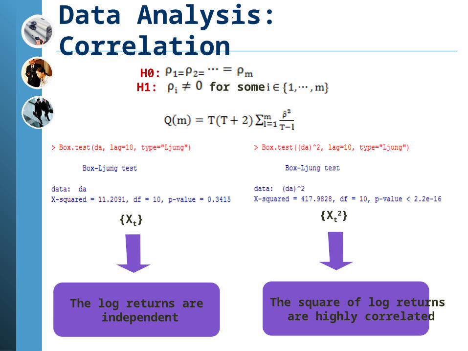
Data Analysis: Correlation

{Xt}{Xt

2}

The log returns are independent

The square of log returns are highly correlated

.

H0:H1: for some

.

Data Analysis : Heavy tail

Density function of exchange rate Normal-QQ plot

Model Setup

GARCH Model

Model Setup

Forecast of GARCH Model

.

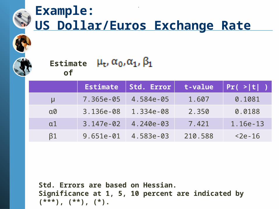
Example:US Dollar/Euros Exchange Rate

Estimate Std. Error t-value Pr( >|t| )

μ 7.365e-05 4.584e-05 1.607 0.1081

α0 3.136e-08 1.334e-08 2.350 0.0188

α1 3.147e-02 4.240e-03 7.421 1.16e-13

β1 9.651e-01 4.583e-03 210.588 <2e-16

.

Estimate of

Std. Errors are based on Hessian. Significance at 1, 5, 10 percent are indicated by (***), (**), (*).

Example:US Dollar/Euros Exchange Rate

Residuals Tests

The Ljung-Box Test are performed for standardized residuals and squared standardized residuals respectively

Trading strategy

Simulate data (ACF)

ACF of historical return ACF of simulated return

Green:| rt | Red: rt ^2 Blue: rt

Trading strategy

Take the 10-day historical volatility (HV) reading.

Take the 50-day historical volatility (HV) reading.

If (VAR(10) < 0.5*VAR(50)) Display(“a big move is likely near!”)

Trading strategy

Using historical data to test:

If(VAR(+n)>VAR(-10))

The strategy is efficient

VAR(-10):volatility between trading signal and10 days before the trading signal VAR(+n):volatility between trading signal and n days after the trading signal

Trading strategy

n VAR(+n) > VAR(-10)

1 0.4194

2 0.5161

3 0.6419

4 0.7161

5 0.7548

6 0.7871

7 0.8161

8 0.8419

9 0.8484

10 0.8581

Trading strategy

Make an assumption:

when we face the trading signal : exchange our US dollar to Euro dollar at current time t. exchange Euro dollar back to US dollar n days after.

By using the historical 3024 days’ exchange rate data,

the program gave us 310 trading signals.

Trading strategy n Probability of making profit

1 0.4645

2 0.4645

3 0.4484

4 0.4677

5 0.4806

6 0.4806

7 0.5065

8 0.4968

9 0.5161

10 0.4935

11 0.5129

12 0.5290

13 0.5484

14 0.5290

15 0.5355

Trading strategy

Property of GARCH:

Large shocks tend to be followed by another large shock;

Small shocks tend to be followed by another small shock.

Trading signal

Market will volatile in next days

Trading strategy

Problems we faced by now

Know some significance moves are about to take place.

Not sure what the direction will turn out to be.

using STRADDLE or STRANGLE

Trading strategy

Straddle: purchase the same number of call and put options at

the same strike price with the same expiration date.

Strangle: purchase the same number of call and put options at

different strike prices with the same expiration date.

Trading strategy

Steps of trading:Straddle : Buy an ATM (At-The-Money) Put Buy an ATM CallStrangle: Buy an OTM (Out-The-Money) Put Buy an OTM Call

Trading strategy

Risk and Reward : The maximum risk of a Straddle/ Strangle is equal to the

amount that you paid for the two option contracts. If the stock moves nowhere, and volatility drops to nothing, you lose.

The reward is that same as for calls and puts - unlimited.

Trading strategy

Tricks to buy the straddle/ strangle

Buy options while volatility is relatively slow Sell as volatility increase either just before a news report or

soon after.

www.themegallery.com

LOGO