1

Seismic envelope inversion and modulation signal model

Ru-Shan Wu, Jingrui Luo, and Bangyu Wu

ABSTRACT

We first point out that envelope fluctuation and decay of seismic records carries ULF (ultra-low

frequency, i.e. frequency below the lowest frequency in the source spectrum) signals which can

be used to estimate the long-wavelength velocity structure. We then propose to use envelope

inversion for the recovery of low-wavenumber components of media (smooth background) so

that the initial model dependence of waveform inversion can be reduced. We derive the misfit

function and the corresponding gradient operator for envelope inversion. In order to understand

the long-wavelength recovery by the envelope inversion, we suggest a nonlinear seismic signal

model: the “modulation signal model” as the basis for retrieving the ULF data and discuss the

nonlinear scale separation by the envelope operator. To separate the envelope data from the

wavefield data (envelope extraction), a demodulation operator (envelope operator) is applied to

the waveform data. Numerical tests using synthetic data for the Marmousi model demonstrated

the validity and feasibility of the proposed approach. The final results of combined EI+WI

(envelope-inversion for smooth background plus waveform-inversion for high-resolution

velocity structure) can deliver much improved results than the regular FWI (Full Waveform

Inversion) alone. Furthermore, to test the independence of envelope to the source frequency-band,

we use a low-cut source wavelet (cut from 5Hz below) to generate the synthetic data. The

envelope inversion and the combined EI+WI show no appreciable difference from the full-band

source results. The proposed envelope inversion is also an efficient method with very little extra

work compared with conventional FWI.

INTRODUCTION

It is known that the lack of ultra low-frequency data leads to the difficulty in recovering long-

wavelength background structure and therefore to the starting-model dependence of full

waveform inversion (FWI) (for a review see Virieux and Operto, 2009). Traditionally, the

starting model for FWI is provided by some other methods such as traveltime tomography

(including ray-based or wave-based, first-arrival traveltime tomography and reflection traveltime

tomography) and velocity analysis. Within FWI, long offsets, multi-scale inversion has been

developed to reduce the starting model dependence (Bunks et al., 1995; Pratt et al., 1996, 1998;

Sirgue and Pratt, 2004; Ravaut et al., 2004; Plessix et al., 2010, Vigh et al., 2011, Baeten et al.,

2013). Multi-scale inversion is a cascade inversion starting from the lowest frequency available

for the recovery of the largest scale possible. Recent development of low-frequency land source

(down to 1.5 Hz) has allowed multi-scale FWI to use 1-D smooth starting model (Baeten et al.,

2013). They showed that the lowest frequency band (1.5 – 2.0 Hz) is crucial in recovering the

correct long-wavelength background velocity structure. However, in general, the ultra-low

frequency sources are not available and the standard seismic records can go down only to about

2

5Hz. Therefore, starting model is still a pressing problem for FWI. Shin and Cha (2009) has

performed inversion in the Laplace-Fourier domain using seismic data below 5Hz, to estimate

the smooth, large-scale velocity structure. A recent trend is that by introducing some extra terms

in the misfit functional, FWI can incorporate into its framework some other inversion methods,

such as traveltime tomography or inversion (Mora, 1989; Clément et al., 2001; Xu et al., 2012;

Ma and Hale, 2013; Wang et al., 2013) and velocity analysis (Biondi and Almomin, 2012, 2013;

Almomin and Biondi, 2012; Tang et al., 2013).

In this paper, we extract the ULF (ultra-low frequency) signals contained in seismic trace

envelopes and apply to the recovery of long-wavelength background structure without the use of

low-frequency sources which are expensive or unavailable. Normalized integration method

(Chauris et al., 2012; Donno et al., 2013) has used the normalized time integration of the squared

waveform data as a new type of data for least-square minimization. However, much information

of the envelope function has been lost due to the integration operator. We demonstrate that

envelope fluctuation and decay of seismic records carries ULF signals but inaccessible from the

conventional linear convolution signal model. In order to extract the envelope data from the

wavefield data and keep the useful information, we need to perform a nonlinear operation using

demodulation operator. For inversion we derive the gradient operator for envelope data and

perform iterative inversion to obtain a smooth background model. Then we use the smooth

model from envelope inversion as the starting model of waveform inversion to recover the high-

wavenumber components of the model. Comparing to the linear multi-scale inversion of FWI,

this is a nonlinear two-scale inversion in which the nonlinear scale separation is done by the

envelope operator. The other advantage of the envelope inversion is its independence to the

source wavelet. We use a low-cut source wavelet (cut from 5Hz below) to generate the synthetic

data. The envelope inversion and the combined EI+WI show no appreciable difference from the

full-band source results. Numerical tests using the Marmousi model demonstrated the validity

and special features of the approach.

ENVELOPE INVERSION

Review of conventional FWI in the time domain

FWI (Full Waveform Inversion) can retrieve information of subsurface by fitting the difference

between the recorded data obsd and the simulated data synd with the proposed model. The classical

least squares misfit functional is given by:

2

0

2

0

1( ) ( )

2

1 = [ ( ) ( )]

2

T

syn obs

sr

T

sr

d d dt

y t u t dt

d

(1)

Where obsu d is the observed wavefield, syny d is the synthetic wavefield. The summation

is over all the sources and receivers.

The goal is to obtain the model parameter m , which can be updated as follows:

3

1n n n nm m (2)

where n is the step length in the thn iteration, n corresponds to the updating direction which

can be obtained from the gradient of the misfit function, so the gradient of the misfit function

with respect to the model m must be calculated first.

Consider velocity v as the model parameter, the gradient of the misfit function with respect to v

can be obtained by:

0

( )[ ( ) ( )]

T

sr

y ty t u t dt

v v

(3)

Introduce an operator J (Jacobian) and a vector (data residual) η , where

( )

, = ( ) ( )y t

y t u tv

J η (4)

then equation (3) can be written as

T

v

J η (5)

The Jacobian J is also called the linear Fréchet derivative. It is known that this gradient can be

calculated by zero-lag correlation of the forward propagated source wavefields and the backward

propagated residual wavefields η (Lailly, 1983; Tarantola, 1984; Pratt et al., 1998; Pratt, 1999).

Misfit functional and gradient operator for envelope inversion

Now we define the misfit functional and derive the corresponding gradient operator for the

envelope inversion. Here the “data” to be used in the misfit functional are the trace envelopes,

not directly the traces (waveforms). Bozdag et al. (2011) have discussed the envelope misfit

functional and its use in the kernel sensitivity analysis of global seismic tomography. However,

their purpose is to use the instantaneous amplitude and phase information of individual arrivals,

such as the first P or S arrivals, so they apply a short time-window to the traces for isolating the

chosen arrivals. For our envelope inversion, we need to extract and treat the envelope of the

whole trace.

We adopt the power objective functional to minimize the residual:

2 2

0 0

2

2 2 2 2

0

2

0

1 1( )

2 2

1( ) ( ) ( ) ( )

2

1

2

T Tp pp psyn synobs obs

sr sr

p pT

H H

sr

T

sr

d d dt e e dt

y t y t u t u t dt

E dt

d

(6)

4

where e is the envelope function, u and y are the observed and synthetic waveforms respectively,

Hu and Hy are the corresponding Hilbert transforms. “E” is the instant envelope data residual

and the summation is over all the sources and receivers. p is the power for the envelope data, it

can be any positive numbers. The extraction of the envelope function and the information

contained in envelopes will be discussed in details in next section. The gradient operator can be

derived from the partial derivative of the misfit with respect to the model perturbations as

follows (for detailed derivation, see Appendix):

2 2

0

22 2

0

2

0

2

( ) ( )

( )( ) = ( ) ( ) ( ) ( )

( )( ) = ( ) ( )

( ) = ( ) ( )

p

T H

sr

pTH

H H

sr

T p Hsyn H

sr

psyn H sy

y t y tE dt

v v

y ty tp E y t y t y t y t dt

v v

y ty tp E e y t y t dt

v v

y tp Ey t e H Ey t e

v

2

0

2 2

0

( )

( ) = ( ) ( )

T pn

sr

T p psyn H syn

sr

y tdt

v

y tp Ey t e H Ey t e dt

v

(7)

We introduce the Fréchet derivative operator (matrix) J and the effective residual vector η ,

defined as

2 2( ), = ( ) ( )p p

syn H syn

y tEy t e H Ey t e

v

J η (8)

So equation (7) can also be written as a matrix equation

T

v

J η (9)

This envelope inversion can also be implemented using back propagation method, and the term

in the square brackets serves as the effective residual, which is the envelope residual riding on

the carrier signal (modulation). Note that operator J includes a backpropagation operator and a

virtual source operator (See Pratt et al., 1998). From the above equations, we see that the L-S

(least-square) residual is calculated using envelope data, but the backprojection of the envelope

residual to the model space is done by backpropagation using the carrying signal with the

envelope residual riding on its shoulder. Based on the above equations, envelope inversion

algorithm can be developed following the algorithm of time-domain waveform inversion.

To see the effect of the parameter p , we rewrite the misfit function in equation (6) as follow:

5

2

0

2

0

2

0

1( ) ( )

2

1( )

2

1( ) ( )

2

T ppsyn obs

sr

W ppsyn obs

sr

W ppsyn obs

sr

e e t dt

e e d

e e d

d

(10)

Calculate the gradient operator, we get:

0

( )( ) ( )

pW synpp

syn obssr

ee e d

v v

(11)

Since syne is a function with respect with y and Hy , using the chain rule we know that the above

equation can be written in the following form:

0

( ) ( )( ) ( )

p pW syn synpp H

syn obsHsr

e e yye e d

v y v y v

(12)

Figure 1 shows two traces generated from the Marmousi model. The top panel are the original

traces; the middle panel are trace envelope in the time domain with different value of p (the

amplitudes have been normalized); the bottom panel are the trace envelope in the frequency

domain with different value of p (the amplitudes have been normalized). We see that different

values of power p of envelope data have the effect of preconditioning the data in both the time

and frequency domains. In the time domain higher power p put heavier weight on the energetic

arrivals, in this case (acoustic wave) earlier envelope arrivals, especially the direct arrivals

(including turning waves); while in the frequency domain, heavier weight on the low-frequency

envelope data. We tested three cases, p = 1, 2, 3. The parameter p = 3 diminish the later arrivals

too much and the inversion cannot penetrate to the depth. Therefore, in applications we use only

p = 1, 2. In next section, we show that p = 2 is a good choice for the Marmousi data set, which

provides a good balance on windowing the data for stable inversion to recover the long-

wavelength background velocity structure.

INFORMATION IN THE ENVELOPE AND THE MODULATION SIGNAL MODEL

Envelope operator (demodulation operator)

In equation 6 we have introduced the envelope function for the misfit functional. The envelope

function is extracted from the waveform data by an envelope operator (or demodulation

operator). The envelope operator ( )f t is consisted of two steps:

(1) Analytic transform of trace f t

a Hf t f t iH f t f t if t (13)

6

(a)

(b)

Figure 1 Data traces generated from Marmousi model and their envelopes with different powers (different values of

p) in both the time domain and frequency domain.

7

where ( )H f t is the Hilbert transform of a real function f, and af is the analytic signal (complex)

corresponding to f.

(2) Take magnitude of the analytic signal

22 2 2 2 2 2

2

( ) ( ) Re( ] [Im( ] ( ) ( )

( ) ( )

f a a a H

f f

t f t f t f t f t f t f t

t sqrt t

(14)

Now we discuss the properties of the envelope operator and information contained in envelopes.

Since envelope operator contains a square-root operator, it is a nonlinear operator (nonlinear

filtering). From the modulation theory in signal processing (e.g. Robinson et al., 1986), we see

that the envelope operator is equivalent to a demodulation operator if we consider a seismogram

as a modulated signal: the low-frequency envelope is the modulation signal and the high-

frequency reflection waveforms as the carrier signal. We will discuss the signal model in the next

subsection. But let us know concentrate on the properties of the extracted envelopes. From the

modulation theory we know that amplitude modulation is a nonlinear operation, and the

modulation frequency is riding on the shoulders of the carrying frequency, as show schematically

in Figure 2. Although the modulation frequency may be very low, it does not show up in the

corresponding low frequency range in the frequency-domain representation of the modulated

signal. In this Figure, (a) is the modulation signal (the envelope); the carrier signal is a sinusoidal

signal with a carrier frequency of 8Hz, (b) is the modulated signal which is the product of the

modulation signal and the carrier signal; (c) and (d) is the spectra of the modulation signal and

the modulated signal respectively (the amplitudes have been normalized). Only the nonlinear

demodulation operator can extract the low-frequency information coded in the envelope.

Figure 3(a) shows a shot profile of waveform data (top) and envelope data (bottom) from the

synthetic data set of the Marmousi model (see next section); The corresponding waveform

spectra (top) and envelope spectra (bottom) are plot in Figure 3(b). We clearly see that the

envelope data have ULF spectra compared with the waveform data. From Figure 1 and 3, we can

also see that envelope shapes are different for different parts of the traces. For the early arrivals

of near offsets, the envelopes look like individual envelopes of the source wavelet; however, for

later arrivals and even early arrivals of far offsets, the envelopes become continuous fluctuations

due to the interference between many arrivals and the nonlinearity of the envelope operator. The

match of envelope data residual may avoid the high-frequency cycle skipping, reduce local

minima and decrease the sensitivity to high-frequency noises.

Modulation signal model

In order to better understand the nonlinear nature of the envelope operator and its effects on

information extraction from seismograms, we first discuss the modulation signal model for

surface reflection seismic data.

In surface reflection survey, the data set (wavefield records) is composed of direct arrivals

(including turning waves) and scattered waves from subsurface reflectors. For the formation of

8

(a) (b)

(c) (d)

Figure 2 (a) The modulation signal; (b) the modulated signal; (c) the spectra of the modulation signal (with a carrier

frequency of 8Hz); (d) the spectra of the modulated signal.

reflection data, the roles of forward scattering and backscattering are very different from each

other. Forward scattering only modifies the Green’s function (propagator) of the background

medium (smooth part), while backscattering of reflectors is actually responsible for the

generation of reflection signals.

In the frequency domain the wave field measured on the surface can be modeled as:

0, , , , , ,scr s r s r sp p p x x x x x x (15)

where 0 , , , ,r s r sp g x x x x is the direct wavefield in the background medium (including

turning waves), and ,scr sp x x is scattered field received by geophone at rx due to a source at sx .

Now we discuss the seismograms formed by backscattered waves, which can be modeled as:

9

(a) (b)

Figure 3 (a) A shot profile of waveform data (top) and envelope data (bottom); (b) waveform spectra (top) and

envelope spectra (bottom). The data are from the synthetic data set of the Marmousi model.

, , ( ) , , ( )bscr s M s M rS

p s g g dS x x x x x x x x (16)

where S represents all the reflection surfaces in the model space, Mg is the modeling Green's

function which is a full-wave Green's function, ( )s is the source spectrum and x is scattering

coefficient of the reflector element. The full-wave Green's function can be decomposed into a

primary-wave part and a multiple-wave part:

M F mulg g g (17)

where Fg is the forward-scattering Green's function, which includes all the forward-scattering

effects (the transmission mode), such as refraction, diffraction, geometric spreading and focusing

effects and therefore contains the average velocity information along the propagation path; while

mulg contains multiply scattered waves from other scatterers. To simplify the treatment, we

consider only the primary reflections, so mulg is neglected. The approximation is similar to the De

Wolf approximation (De Wolf, 1971, 1985; Wu, 1994, 2003). We know that the scattering

models for forward-scattering and backscattering are very different, and therefore the

information contained in the reflection series x and in the forward scattering approximated

10

Green's function Fg represents different properties of medium perturbations. In the case of direct

arrivals, Fg contains velocity perturbations along the propagation path; while for reflected

arrivals, x corresponds to local reflectivity due to impedance jump (velocity jump for acoustic

media with constant density).

Assuming there are totally L’s interfaces (including reflector surfaces) and each interface has lM

elements (after discretization), so the total number of scattering elements is1

L

l

l

N M

. Then the

primary backscattered field (discretized version of (16)) can be modeled as reflection series

1

, , ( ) , , , , ( )N

bscr s F i s F r i i i

i

p s g g ds

x x x x x x x x (18)

For simplicity, we take the reflection coefficients as frequency-independent. The frequency-

domain and time-domain solutions for reflected signals can be written as:

, , ( ) , , , ,

, , ( ) , , , ,

bscr s F i s F r i i

i

bscr s F i s F r i i

i

p s g g

p t s t g t g t

x x x x x x x

x x x x x x x

(19)

where “*” denotes time convolution. Green’s functions can be expressed in a form

( ) [ ( )]

( ) [ ( )

,

, ]

,

,

F i s is s

r r

i

F i r i i

g g

g

exp i

exp ig

x x x x

x x x x (20)

where s and r are the corresponding time-delays due forward-scattering along the source path

and receiver path, respectively. We define a propagator

( ) ( ) [ ( ); )], (, s r ssr i i rs r iexpG ig g x x x x x (21)

so the reflection seismograms can be modeled as reflection time series

, , , ; , ; , ,)

, )

(

(

bscr s w r s i sr i s r i

i i

i i i

p t R t G t t

t t

s t

x x x x x x x x

x

(22)

Here the spatial distribution of reflectors in the 3-D space is transformed into a time series by a

distance-time correspondence in a background medium (e.g. homogeneous medium). The above

equation is the traditional convolution signal model (Robinson, 1957; Robinson et al., 1986), in

which the propagator (Green's function pairs) , ; ,sr i s rG t x x x only modify the travel-times and

amplitudes of the reflection events, and the signal spectrum is mainly determined by the source

wavelet. Both the amplitude and phase functions of the propagator srG are smoothly varying

11

functions. The neglect of mulg is equivalent to the drop of “reverberation waveform” in the

convolution model (Robinson et al., 1986). We see that the propagator, although carrying smooth

medium information, can only modify the source spectrum. Based on the linear signal model, we

are restricted to only access the information provided within source spectra. This convolution

model is good for seismic imaging, since it provides the mathematical model for resolution

analysis and resolution enhancement (such as deconvolution) in high-resolution imaging.

However, depending on the information you want to extract from the seismic records

(seismograms), one can define different signal models. In fact, seismograms have much rich

information than the convolution model predicts. For seismic inversion, we need the low-

frequency information contained in seismograms for the recovery of long-wavelength

background velocity structure. We see from the above analysis that there is low-frequency

information coded into the envelope fluctuation and decay of seismograms, but not accessible

from linear convolution model. The problem is how to take use of the information associated

with Fg coded in the envelope for the estimate of long-wavelength velocity structure in

waveform inversion. Demodulation operator can peel off the envelope from the seismograms,

and therefore can in certain way decode the low-frequency information not reachable by linear

methods. To understand the demodulation operator and its effect to the signal spectra, we need to

consider the modulation signal theory.

We reformulate and redefine the signal model of equation (18) as a modulation model. Since the

propagator , ; ,sr i s rG t x x x is a smooth function of time with respect to the reflection series, so

the signal model (18) can be rewritten as:

( )

( )

, , ; , ( , )

; ,

( , )

bscr s sr s r i i

i

wsr s r

i

i

w i

p t G t t

G t t

t

s t

s t t

x x x x x

x x

x

(23)

where w t is the reflectivity series with the source wavelet signature, which is considered as the

carrier signal, while srG is the modulation signal. The high-frequency carrier signal is modulated

by the earth medium though wave propagation (only forward-scattering involved). We can

consider the reflection series (23) as a Modulation-convolution signal model, or simply as a

modulation signal model for the reflection series if we are concern mainly on the low-

wavenumber background recovery (This signal model has been briefly discussed in Wu et al.,

2012, 2013). In fact we can say that the carrier and the modulation signals contain quite different

information about the earth media. The carrier w t is formed by impedance discontinuities

convolved with the source wavelet; while the modulator srG contains mainly the information on

the smoothed medium velocity structure (under the forward-scattering approximation).

Now we include the direct arrivals, which can be written as:

0, , , , , ,

, , ( ( ), , )

d dscr s r s r s

d dr s r s

p p p

p t g t s t

x x x x x x

x x x x (24)

12

where

( , , ) ( , , )d i t dr s r sg t d e g x x x x (25)

is the Green's function for the direct arrival and is assumed to be a much slower time-varying

function than the source wavelet. Since the direct arrivals are single arrivals or sparse arrivals, so

the convolution can be approximated by product. Including the direct arrivals (24) and the

reflection series (23), the modulation signal model for the whole seismogram can be expressed as:

, , ( , , ) ; ,( )dr s r s sr s r ws tp t g t G t t x x x x x x (26)

For a seismogram including the reflection series, we can view it as a product of two functions: a

carrier signal and a modulator. For the direct arrivals, the carrier is the source wavelet, and the

modulator is the direct propagator (Green's function); for the reflect series, the carrier is w t

and the modulator is the propagator ; ,sr s rG t x x . If we apply a long-wavelength velocity

perturbation to a given model, but keep the impedance jumps unchanged, then the propagator

will change, resulting in a modulation in both amplitude and phase to the original reflection

series. After demodulating the traces, the envelope changes (residuals) contain the long-

wavelength information of the velocity perturbation. This provides the signal basis for long-

wavelength background recovery.

Now we look at the consequence and effect of demodulation operator applied to the modulation

model (equation (26)). We apply the Hilbert transform product theorem, i.e. the Bedrosian-

Brown theorem (Bedrosian, 1962; Brown, 1986), to the trace model (26),

, , ( , , ) ; ,

( , , ) ;

( )

( ) ,

dr s r s sr s r

dr s sr

w

s r w

H p t H g t Gs t t

g t H G t H t

t

s t

x x x x x x

x x x x (27)

Since the propagator functions ( , , )dr sg t x x and ; ,sr s rG t x x are low-pass functions (slowly

varying function) (under the forward-scattering approximation) and satisfies the Brown’s

condition for demodulation (ibid), so it can be pulled out of the Hilbert transform. Therefore, the

envelope function of the seismic traces can be approximated by

22 2 2

2 222 22

22 2 2

( ) ( ) ( ) ( )

( ) ( )( )

( )( () )

a H

dH sr

dsr

w w

w

t p t p t p t

g t s t G t ts t

s t t

H t

g t G t

(28)

where 2 ( )s t is the squared envelope of the source wavelet. In deriving the above equation, we

neglected the cross-talk between the direct arrival energy and the reflection series energy. This

assumption is valid for near and medium offsets due to the travel-time difference. For far offsets,

the approximation may not be valid and needs further study. However, this approximation is not

critical for envelope extraction. We see that taking envelope of seismograms (demodulation) is

13

equivalent to the application of a nonlinear signal filtering, resulting in the extraction of low-

frequency information coded in the seismograms. For direct arrivals (the first term in the right-

hand side), the resulted envelope-gram (envelogram) has the effect of using a low-resolution

wavelet (a Gaussian pulse) to replace the original high-frequency wavelet (Ricker wavelet). For

reflection series (The second term in the right-hand-side), 2 ( )w t will extract only the low-

frequency part of the carrier signal ( )w t . We also noticed that the envelope operator keeps the

long-wavelength information riding on the propagator srG untouched. In this way, the high-

wavenumber reflection information is peeled off and only low-wavenumber background is kept

in the envelograms.

Nonlinear scale separation by envelope operator

It is well-known that seismic data has a wavenumber gap (or a scale gap) in terms of subsurface

structure inversion. That is the lack of intermediate wavenumber (medium-scale) information

about the subsurface media in the data (Claerbout 1983; Jannane et al. 1989; Mora, 1989; Ghosh

2000; Latimer et al. 2000; Plessix et al., 2012; Baeten et al., 2013). For 3-D earth structure, this

gap is the combined results of limited acquisition frequency-band and limited observation

aperture. For surface reflection survey with limited acquisition aperture, the gap is mainly caused

by the lack of low-frequencies in source spectra (e.g., Latimer et al., 2000; Baeten et al., 2013).

Therefore, substantial efforts have been paid to develop low-frequency sources. Big gun arrays

and a deeper towing depth can provide low frequencies down to as low as 2Hz, but even lower

frequencies are still needed (Vigh et al, 2011; Baeten et al., 2013 ). Recently, low-frequency land

source (vibrator with nonlinear frequency sweep) has been reported (Plessix et al., 2012; Baeten

et al., 2013) which can extent the low-frequency end to 1.5 Hz. FWI using the corresponding

data showed improved low-wavenumber background recovery. Due to the availability of low-

frequency data, they could use a 1-D smooth starting model in their multi-scale inversion scheme.

They showed that the lowest frequency band (1.5 – 2.0 Hz) is crucial in recovering the correct

low-wavenumber background velocity structure.

As we mentioned above, the linear scale separation is usually realized by a multi-scale inversion:

the large-scale recovery is done using the low-frequency data and the smaller scales are

recovered from the high-frequency data subsequently. In this linear approach, the expensive low-

frequency source is a necessary and critical armament for success. In the following we discuss

the nonlinear scale separation through envelope operator.

To simplify the scale analysis, in the following we mainly discuss the scale response for vertical

structural variations as in previous discussions (Jannane et al., 1989; Baeten et al., 2013). From

equation (28) and Figure 2-3, we see that the envelope operator can peel off the low-frequency

envelope from the waveform traces. The low-frequency nonlinear extraction in fact separates the

large-scale response which is coded in the envelope, from the waveform data which are the band-

limited response to the medium perturbation. This is very different from the concept of linear

scale separation which depends on the linear correspondence between the signal frequency and

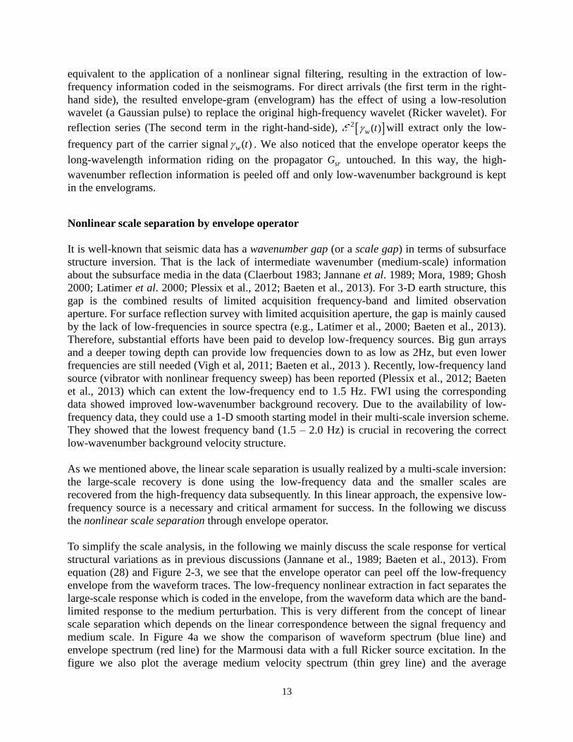
medium scale. In Figure 4a we show the comparison of waveform spectrum (blue line) and

envelope spectrum (red line) for the Marmousi data with a full Ricker source excitation. In the

figure we also plot the average medium velocity spectrum (thin grey line) and the average

14

velocity perturbation (medium velocity subtracts the background velocity) spectrum (dotted line).

In order to see the correspondence of medium wavenumber spectra to the data frequency spectra,

we perform a z-t transform using the known velocity structure. The medium spectrum shown on

the figure is the average over all the vertical profiles. The same has done for the perturbation

spectrum. Form Figure 4a, we see that for the waveform data, the low-frequency spectral

components are missing so the long-wavelength part of the perturbation spectrum is not covered.

Compared with envelope spectrum, we see the complimentary role of envelope data which has

strong low-frequency components but has very weak high-frequency components. This property

of the envelope function can reduce the cycle skipping and local minima problems of waveform

data and can recover the long-wavelength components of the perturbation structure as show in

the next section for the Marmousi model. Of course its limitation needs to be further studied.

Because of the nonlinear nature of the envelope operator, the low-frequency contents of the

envelope data do not tightly depend on the source spectrum, which is a sharp contrast to the

conventional FWI. In Figure 4b we plot a similar spectral comparison as in Figure 4a, but using a

low-cut Ricker source. When generating synthetic seismograms, the source wavelet was filtered

with a 5 Hz low-cut taper. From the spectrum of waveform data thus generated, we see very little

energy exists below 5 Hz. Later in the FWI tests we can see much worse results than the full-

band source because of the lack of low-frequency energy. However, the spectrum of the envelope

data (average over all the traces) does not show too much difference from the full-band source

case. This demonstrates the nonlinear nature of the envelope extraction, which does not have the

linear correspondence between the source spectrum and the data spectrum. Later in the inversion

test section, we will show that the inversion results for these two cases are very similar, showing

the independence of envelope inversion to the source spectra.

(a) (b)

Figure 4 (a) Comparison of waveform spectrum and envelope spectrum for the Marmousi data with a full Ricker

source excitation; (b) Same as (a) but with a low-cut source excitation. The low-cut source is obtained by a 5Hz low-

frequency taper.

This kind of nonlinear scale separation is similar to the Laplace domain inversion (Shin and Ha,

2008) and the normalized integration method (Chauris et al., 2012; Donno et al., 2013). For

15

linear scale separation in the multi-scale inversion method, the inversion theory is based on the

Born modeling. However, for nonlinear scale separation, the forward modeling theory for the

long-wavelength part is not the Born modeling. The forward modeling theory for envelope

inversion needs further investigation, which may provide more insight on the benefit and

limitation of the envelope inversion.

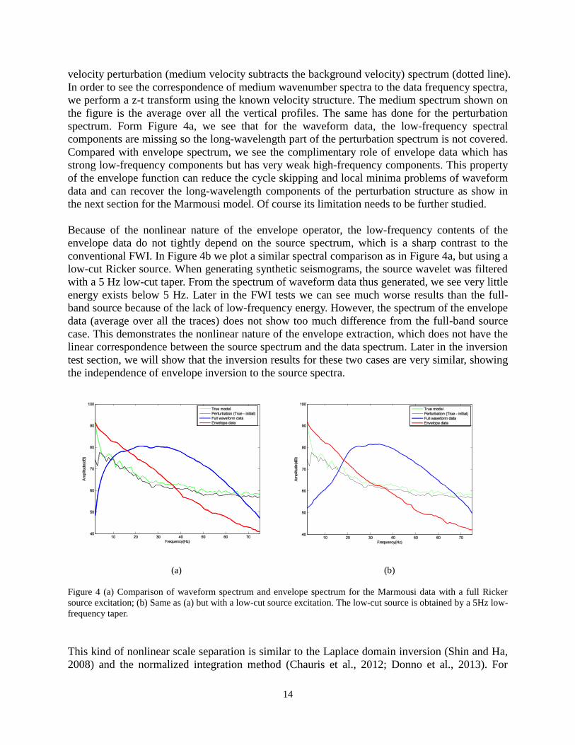
INVERSION TESTS WITH THE MARMOUSI MODEL

The data were generated by a FD algorithm with an acquisition system composed of 50 shots

evenly distributed along the surface. We used total 228 receivers across the surface for each shot.

The true model is shown in Figure 5(a). A linear gradient model is used as the initial model

(Figure 5(b)).

(a) (b)

Figure 5 (a) True Marmousi model; (b) linear gradient initial model.

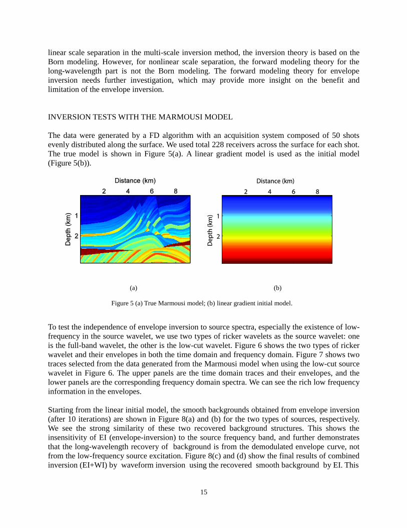
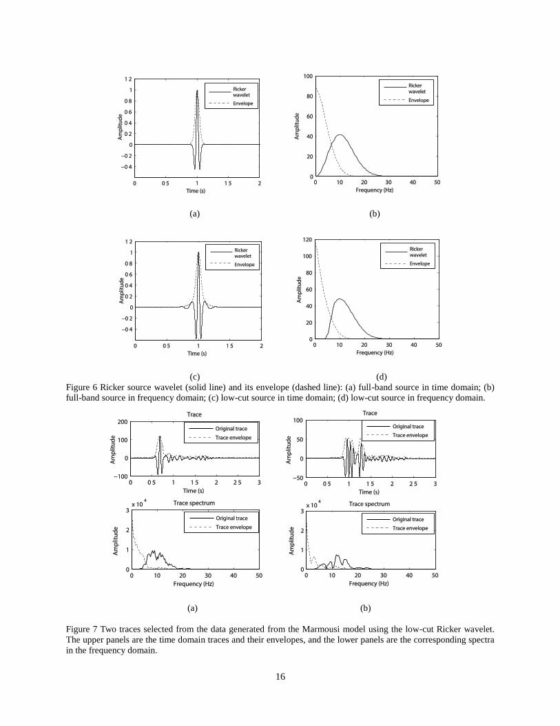
To test the independence of envelope inversion to source spectra, especially the existence of low-

frequency in the source wavelet, we use two types of ricker wavelets as the source wavelet: one

is the full-band wavelet, the other is the low-cut wavelet. Figure 6 shows the two types of ricker

wavelet and their envelopes in both the time domain and frequency domain. Figure 7 shows two

traces selected from the data generated from the Marmousi model when using the low-cut source

wavelet in Figure 6. The upper panels are the time domain traces and their envelopes, and the

lower panels are the corresponding frequency domain spectra. We can see the rich low frequency

information in the envelopes.

Starting from the linear initial model, the smooth backgrounds obtained from envelope inversion

(after 10 iterations) are shown in Figure 8(a) and (b) for the two types of sources, respectively.

We see the strong similarity of these two recovered background structures. This shows the

insensitivity of EI (envelope-inversion) to the source frequency band, and further demonstrates

that the long-wavelength recovery of background is from the demodulated envelope curve, not

from the low-frequency source excitation. Figure 8(c) and (d) show the final results of combined

inversion (EI+WI) by waveform inversion using the recovered smooth background by EI. This

16

(a) (b)

(c) (d)

Figure 6 Ricker source wavelet (solid line) and its envelope (dashed line): (a) full-band source in time domain; (b)

full-band source in frequency domain; (c) low-cut source in time domain; (d) low-cut source in frequency domain.

(a) (b)

Figure 7 Two traces selected from the data generated from the Marmousi model using the low-cut Ricker wavelet.

The upper panels are the time domain traces and their envelopes, and the lower panels are the corresponding spectra

in the frequency domain.

17

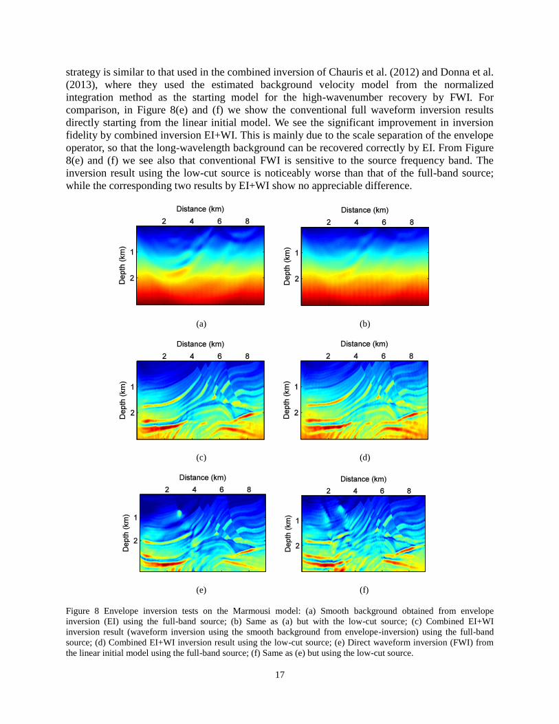
strategy is similar to that used in the combined inversion of Chauris et al. (2012) and Donna et al.

(2013), where they used the estimated background velocity model from the normalized

integration method as the starting model for the high-wavenumber recovery by FWI. For

comparison, in Figure 8(e) and (f) we show the conventional full waveform inversion results

directly starting from the linear initial model. We see the significant improvement in inversion

fidelity by combined inversion EI+WI. This is mainly due to the scale separation of the envelope

operator, so that the long-wavelength background can be recovered correctly by EI. From Figure

8(e) and (f) we see also that conventional FWI is sensitive to the source frequency band. The

inversion result using the low-cut source is noticeably worse than that of the full-band source;

while the corresponding two results by EI+WI show no appreciable difference.

(a) (b)

(c) (d)

(e) (f)

Figure 8 Envelope inversion tests on the Marmousi model: (a) Smooth background obtained from envelope

inversion (EI) using the full-band source; (b) Same as (a) but with the low-cut source; (c) Combined EI+WI

inversion result (waveform inversion using the smooth background from envelope-inversion) using the full-band

source; (d) Combined EI+WI inversion result using the low-cut source; (e) Direct waveform inversion (FWI) from

the linear initial model using the full-band source; (f) Same as (e) but using the low-cut source.

18

Figure 9 shows the reduction of L-S residuals with iterations. Compared with FWI (dashed line),

the convergence of EI+WI (solid line) is faster and has avoided the false local minima.

Figure 9 Reduction of L-S residuals with iterations. Comparison of EI+WI (solid line) and FWI (dashed line).

To demonstrate the effect of data power p to the result of envelope inversion, in Figure 10 we

show the result of envelope inversion (EI) with p=1 and the final result of EI+WI. As we

discussed in the previous section, the EI results in this case are much rougher than the case of

p=2 due to the heavier weight on the later arrivals (reflections) and on the high-frequency

components of the envelope data. We know that the backpropagation of envelope data is similar

to energy-pact imaging, so there is no destructive interference, resulting in a noisier image than

the FWI image. Note that even though the EI results of p=1 are very different from that of p=2,

the final result of EI+WI in this case is very similar to the case of p=2. This indicates that long-

wavelength background media recovered in these two cases are fairly close to each other.

(a) (b)

Figure 10 Envelope inversions (EI) with p=1 (a). and the final result of EI+WI (b). Note that even the EI results of

p=1 are very different from that of p=2, the final result of EI+WI in this case is very similar to the case of p=2.

19

CONCLUSION

Envelope fluctuation and decay of seismic records carries ULF (ultra-low frequency) signals

which can be used to estimate the long-wavelength velocity structure. We proposed a nonlinear

seismic signal model: the “modulation model” for retrieving the ULF information in seismic

waveform data. Eenvelope inversion based on least-square minimization of envelope data can

recover the low-wavenumber components of unknown velocity strucutes (smooth backgrounds)

so that the initial model dependence of waveform inversion can be reduced. This is demonstrated

by the Marmousi model tests, in which a 1-D linear grandient starting model is used and the

combined EI+WI (envelope-inversion plus waveform inversion) can correctively recover both

the low- and high-wavenumber structure of the model. The other advantages of the envelope

inversion are its independence to the source wavelet and its low cost (very little extra cost

beyond the regular FWI cost). Futher study is needed for the inversion dependence on reflector

distribution, acquisition aperture, and other limintations of the envelope inversion. The other

important research topic for better understanding the advantages and limitations of envelope

inversion is the forward modeling of envelope formation, which will be investigated in the future

study.

Acknowledgments: We thank Mimi Dai, Jian Mao, Yu Geng, Lingling Ye, Rui Yan, Xiao-Bi

Xie for discussions and helps. The suggestions and comments of reviewers are appreciated. We

thank also the WTOPI members who participated in the discussions during our last year’s annual

WTOPI meeting. This research is supported by the WTOPI Research Consortium at the

University of California, Santa Cruz.

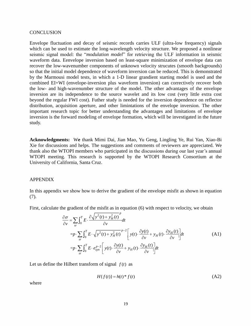
APPENDIX

In this appendix we show how to derive the gradient of the envelope misfit as shown in equation

(7).

First, calculate the gradient of the misfit as in equation (6) with respect to velocity, we obtain

2 2

0

22 2

0

2

0

( ) ( )

( )( ) = ( ) ( ) ( ) ( )

( )( ) = ( ) ( )

p

T H

sr

pTH

H H

sr

T p Hsyn H

sr

y t y tE dt

v v

y ty tp E y t y t y t y t dt

v v

y ty tp E e y t y t dt

v v

(A1)

Let us define the Hilbert transform of signal ( )f t as

{ ( )} ( )* ( )H f t h t f t

(A2)

where

20

1

( )h tt

(A3)

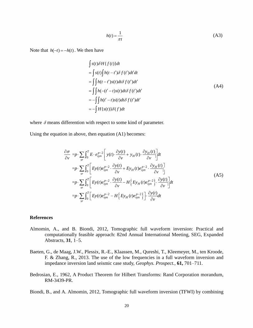
Note that ( ) ( )h t h t . We then have

( ) { ( )}

( ) ( ) ( )

( ) ( ) ( )

( ( ) ( ) ( )

( ) ( ) ( )

{ ( )} ( )

s t H f t dt

s t h t t f t dt dt

h t t s t dt f t dt

h t t s t dt f t dt

h t t s t dt f t dt

H s t f dt

(A4)

where means differention with respect to some kind of parameter.

Using the equation in above, then equation (A1) becomes:

2

0

2 2

0

2 2

0

( )( ) = ( ) ( )

( )( ) = ( ) ( )

( ) ( ) = ( ) ( )

=

T p Hsyn H

sr

T p p Hsyn H syn

sr

T p psyn H syn

sr

y ty tp E e y t y t dt

v v v

y ty tp Ey t e Ey t e

v v

y t y tp Ey t e H Ey t e dt

v v

p

2 2

0

( )( ) ( )

T p psyn H syn

sr

y tEy t e H Ey t e dt

v

(A5)

References

Almomin, A., and B. Biondi, 2012, Tomographic full waveform inversion: Practical and

computationally feasible approach: 82nd Annual International Meeting, SEG, Expanded

Abstracts, 31, 1–5.

Baeten, G., de Maag, J.W., Plessix, R.-E., Klaassen, M., Qureshi, T., Kleemeyer, M., ten Kroode,

F. & Zhang, R., 2013. The use of the low frequencies in a full waveform inversion and

impedance inversion land seismic case study, Geophys. Prospect., 61, 701–711.

Bedrosian, E., 1962, A Product Theorem for Hilbert Transforms: Rand Corporation morandum,

RM-3439-PR.

Biondi, B., and A. Almomin, 2012, Tomographic full waveform inversion (TFWI) by combining

21

full waveform inversion with wave equation migration velocity analysis: SEG Expanded

Abstract.

Doi: 10.1190/segam2012-0275.1

Biondi, B and A. Almomin, 2013, Tomographic full waveform inversion (TFWI) by extending

the velocity model along the time-lag axis, SEG Expanded Abstract, 1031-1034.

Bozdag, E, J., Trampert, and J., Tromp, 2011, Misfit functions for full waveform inversion based

on instantaneous phase and envelope measurements: Geophys. J. Int., 185, 845-870.

Brittan, J., J. Bai, H. Delome, C. Wang and D. Yingst, 2013, Full waveform inversion – the state

of the art, First break, 31, 75-81.

Brown, J.L. Jr., 1986, A Hilbert transform product theorem: Proceedings of the IEEE, 74, 520-

521.

Chauris, H., D. Donno, H. Calandra, 2012, Velocity estimation with the normalized integration

method, : 74th

EAGE Conference & Exhibition, Expanded Abstracts, W020.

Claerbout, J. F., 1985, Imaging the Earth's interior: Blackwell Sci. Pub..

Clément, F., G. Chavent, and S. Gómez, 2001, Migration-based traveltime waveform inversion

of 2-D simple structures: A synthetic example: Geophysics, 66, 845-860.

De Wolf, D. A., 1971, Electromagnetic reflection from an extended turbulent medium:

Cumulative forward-scatter single-backscatter approximation: IEEE Trans. Antennas and

Propagations AP-19, 254–262.

De Wolf, D. A., 1985. Renormalization of EM fields in application to large-angle scattering from

randomly continuous media and sparse particle distributions: IEEE Trans. Antennas and

Propagations AP-33, 608–615.

Donno, D., H. Chauris and H. Calandra, 2013, Estimating the background velocity model with

the normalized integration method, 75th

EAGE Conference & Exhibition, Expanded

Abstracts.

Fichtner, A., Trampert, J., 2011. Resolution analysis in full waveform inversion. Geophys. J. Int.

187, 1604–1624.

Jannane, M., W. Beydoun, E. Crase, D. Cao, Z. Koren, E. Landa, M. Mendes, A. Pica, M. Noble,

G. Roeth, S. Singh, R. Snieder, A. Tarantola, D. Trezeguet, and M. Xie, 1989,

Wavelength of earth structures that can be resolved from seismic reflection data:

Geophysics, 54, 906-910.

Lailly, P., 1983, The seismic inverse problem as a sequence of before stack migrations, in Bednar,

J. B., Redner, R., Robinson, E., and Weglein, A., Eds., Conference on Inverse Scattering:

22

Theory and Application, Soc. Industr. Appl. Math..

Ma, Y. and D. Hale, 2013, Wave-equation reflection traveltime inversion with dynamic warping

and full-waveform inversion: Geophysics, 78, R223-R233.

Mora, P. , 1989, Inversion=migration+tomography. Geophysics, 54, 1575-1586.

Plessix, R., G. Baeten, J. W. de Maag, M. Klaassen, R. Zhang and Z. Tao, 2010, Application of

acoustic full waveform inversion to a low-frequency large-offset land data set, SEG

Expanded Abstract, 930-934.

Pratt, R. G., 1999, Seismic waveform inversion in the frequency domain, Part I: Theory and

verification in a physical scale model: Geophysics, 64, 888–901.

Pratt R.G., Song Z.M., Williamson P.R. and Warner M. 1996. Twodimensional velocity model

from wide-angle seismic data by wavefield inversion. Geophysical Journal International

124, 323–340.

Pratt, R. G., C. Shin, and G. J. Hicks, 1998, Gauss-Newton and full Newton methods in

frequency-space seismic waveform inversion: Geophysical Journal International, 133,

341–362.

Ravaut, C., S. Operto, L. Improta, J. Virieux, A. Herrero and P. Dell’Aversana, 2004, Multiscale

imaging of complex structures from multifold wide-aperture seismic data by frequency-

domain full-waveform tomography: application to a thrust belt, Geophys. J. Int., 159,

1032–1056.

Robinson, E. A., 1957, Predictive decomposition of seismic traces: Geophysics, 22, 767-78.

Robinson, E. A., T. S., Durrani, and L. G., Peardon, 1986, Geophysical signal processing:

Prentice-Hall International.

Shin, C. and Y.H. Ha, 2008, waveform inversion in the Laplace domain, Geophysical J.

International, 173(3), 922-931.

Sirgue, L. and Pratt, R.G. 2004, Efficient waveform inversion and imaging: A strategy for

selecting temporal frequencies. Geophysics, 69, 231–248.

Sirgue, L., Barkved, O.I., Dellinger, J., Etgen, J., Albertin, U. and Kommedal, J.H. 2010, Full-

waveform inversion: the next leap forward in imaging at Valhall. First Break, 28 (4), 65–

70. Shin, C., and Y. H. Cha, 2009, Waveform inversion in the Laplace-Fourier domain:

Geophys. J. Int., 177, 1067-1079.

Tarantola, A., 1984, Inversion of seismic reflection data in the acoustic approximation:

Geophysics, 49, 1259-1266.

23

Tarantola, A., 1987, Inverse problem theory, Elsevier.

Tang, Y., S. S, Lee, A. Baumstein and D. Hinkely, 2013, Tomographically enhanced full

wavefield inversion, 83rd Annual International Meeting, SEG, Expanded Abstracts

Virieux J. and Operto S. 2009. An overview of full waveform inversion in exploration

geophysics. Geophysics 64, WCC1–WCC26.

Vigh, D., J. Kapoor, N. Moldoveanu, and H. Li, 2011, Breakthrough acquisition and technologies

for subsalt imaging: Geophysics, 76, WB41-WB51.

Wang, F., H. Chauris, D. Donno & H. Calandra, 2013, Taking Advantage of Wave Field

Decomposition in Full Waveform Inversion: 75th

EAGE Conference & Exhibition,

Expanded Abstracts.

Wu, R. S., 1994, Wide-angle elastic wave one-way propagation in heterogeneous media and an

elastic wave complex-screen method: J. Geophys. Res., 99, 751-766.

Wu, R. S., 2003, Wave propagation, scattering and imaging using dual-domain one-way and one-

return propagators: Pure and Applied Geophysics, 160(3/4), 509-539.

Wu, R.S., B. Wu and M. Dai, 2012, Ultra-low-frequency information in seismic data： Its

representation and extraction: MIP-report, MIP-23, 69-95, University of California, Santa

Cruz.

Wu, R.S., J. Luo and B. Wu, 2013, Ultra-low-frequency information in seismic data and

envelope inversion: SEG Extended abstract.

Xu, S., D. Wang, F. Chen, Y. Zhang, and G. Lambare, 2012, Full waveform inversion for

reflected seismic data: 74th EAGE Conference & Exhibition, Expanded Abstracts, W024.