wp4.4. combi systems â€“ integrated or external boiler

New Generation of Solar Thermal Systems

SUMMARY (ARIAL 12, BOLD) Side-by-side measurements of the REBUS and the SolvisMax SX-655 solar combi systems are described. Both systems use a condensing gas boiler as auxiliary energy supply system. In one system, the gas boiler is build into the hot water storage tank. The other system uses an external gas boiler. 1. Introduction The document will describe laboratory tests carried out at the Technical University of Denmark on two solar combisystems, one with an integrated boiler and one with an external boiler.

WP4.4. COMBI SYSTEMS –

INTEGRATED OR EXTERNAL BOILER

January 2007 CONTENTS 1. INTRODUCTION 2. SIDE-BY-SIDE MEASUREMENTS OF THE REBUS AND THE SOLVISMAX SX-655 SOLAR COMBI SYSTEMS 3. CONCLUSIONS REFERENCES

NEGST – NEW GENERATION OF SOLAR THERMAL SYSTEMS – is a project financed by the European Commission

TOWARDS NEW STANDARDS FOR ADVANCED STORES – JAN. 2007 page 2 of 7 pages

2. Side-by-side measurements of the REBUS and the SolvisMax SX-655 solar combi systems. The REBUS system is described in detail in /1/. The condensing gas boiler is a Nefit Milton Smartline HR 24 from the Danish company Milton A/S. The boiler is modulating in the interval from 5.7 kW to 23 kW for space heating load and to 28.5 kW for domestic hot water preparation. Figure 1 shows the design of the compact solar combi system units consisting of a technical unit and a hot water storage tank unit and the hydraulic scheme of the system. The volume of the hot water tank is 300 l. The boiler uses the upper 70-80 l.

Figure 1 Right: Design of the compact solar combi system as two 60 x 60 cm units: On the left side a solar tank and on the right side the prefabricated technical unit with integrated condensing natural gas boiler or pellet boiler and all the other components like pumps, switching valves, mixing valves, expansion vessels, plate heat exchanger, controller, etc. Right: Hydraulic scheme of the REBUS solar combi system. Figures from /1/. The SolvisMax system has an integrated gas boiler which is modulating in the interval 5 kW to 20 kW. The total tank volume is 635 l. The upper 136 l are used for heating of domestic hot water. 30 l are reserved for space heating. The remaining 469 litres are reserved for the solar collectors. Figure 2 shows schematic illustration of the heat storage tank of the SolvisMax system and the positions of the temperature sensors used for the investigations.

Solar Store Unit Technical Unit

HW

CW

Space heating

Solar loop

Boiler

S

S

M

Radiators Floor heating

SS

Domestic hot water

Solar Store Unit Technical Unit

HW

CW

Space heating

Solar loop

Boiler

S

S

M

Radiators Floor heating

SS

Domestic hot water



Figure 2 The heat storage tank of the SolvisMax system. Side-by-side measurements of the two systems have been carried out in the test laboratory at the Department of Civil Engineering at the Technical University of Denmark. The SolvisMax system has an auxiliary volume for heating of domestic hot water. Hence the temperature in the top of the SolvisMax tank is kept at a constant high temperature level regardless of the temperature level in the space heating system. The REBUS system does not have an auxiliary volume for domestic hot water. Hence the temperature in the top of the REBUS tank is only a few degrees higher than the required temperature for the space heating system. During the tests, constant space heating loads in the range from 5 kW to 10 kW were drawn from the systems. The solar collector loop and the domestic hot water draw off were not used. Figure 3 shows a schematic illustration of the principle of the space heating system. A mixing valve determines the temperature of the water going to the space heating system (Tflow). The volume flow rate in the space heating system is fixed. The return temperature from the space heating system (Treturn) results from the flow temperature to the space heating system, the volume flow rate and the size of the space heating system.

DHW

SH

AUXILIARY ENERGY

SOLAR

SIDEARM



Figure 3 Schematic of the heating system. Figure 4 and 5 show examples of the temperatures in the SolvisMax and the REBUS system during operation, respectively. From Figure 4 it can be seen that the flow temperature is about 47ºC with a return temperature of about 25ºC. Further, it can be seen that the boiler in the SolvisMax system starts approximately two times per hour, and that the exhaust gas temperature is about 42ºC. Figure 5 shows that the flow temperature in the REBUS system is about 46ºC when the boiler is not in operation and increases to about 52ºC when the boiler is in operation. The exhaust gas temperature is about 48ºC. The REBUS boiler starts about once every hour. The volume reserved for space heating in the SolvisMax system is only 30 l. The space heating volume in the REBUS system is 70-80 l. This explains why the SolvisMax system has more boiler operation periods. The exhaust gas temperature is higher in the REBUS system than in the SolvisMax system because the volume flow rate going through the REBUS boiler is very high. This enables the REBUS boiler to modulate to a low power.

Heating system

to space heating

from space heating

Mixing valve



Figure 4 Temperatures in the SolvisMax system. T1-T10 show the temperatures in the storage tank from top to bottom. Tsidearm is the temperature in the side arm before the heat exchanger. The temperature in the side arm is kept hot (>25ºC) by the pump in the side arm. The explanation for this strategy is that the pump during a domestic hot water draw off is activated by a sudden temperature drop.

Figure 5 Temperatures in the REBUS system.

20

30

40

50

60

70

80

90

15:1

1:02

15:4

6:57

16:2

1:57

16:5

6:57

17:3

1:57

18:0

6:57

18:4

1:57

19:1

6:56

19:5

1:56

20:2

6:56

21:0

1:56

21:3

6:56

22:1

1:56

22:4

6:56

23:2

1:56

23:5

6:56

00:3

1:56

01:0

6:56

01:4

1:56

02:1

6:56

02:5

1:56

03:2

6:56

04:0

1:56

04:3

6:56

05:1

1:56

05:4

6:56

06:2

1:56

06:5

6:56

07:3

1:56

08:0

6:56

08:4

1:56

09:1

6:55

040107 - 050107, Time

Tem

pera

ture

[°C

]

-50

-40

-30

-20

-10

0

10

20

Pow

er fo

r spa

ce h

eatin

g [k

W]

Treturn (SH) T1 T2 T3 T4 T5T6 T7 T8 T9 T10 TexhTsidearm Tflow (SH) Power (SH)

SolvisMax SX-655 Power (SH)

Tflow (SH)

Texh

Treturn (SH)

20

30

40

50

60

70

80

90

15 15 16 16 17 18 18 19 19 20 21 21 22 22 23 23 0 1 1 2 2 3 4 4 5 5 6 6 7 8 8 9

040107 - 050107, Hour

Tem

pera

ture

[°C

]

-50

-40

-30

-20

-10

0

10

20P

ower

for s

pace

hea

ting

[kW

]

Treturn (SH) Tflow (SH) Texh Power (SH)

REBUS

Texh

Tflow (SH)

Power (SH)

Treturn (SH)



The measurements are carried for the systems operated in space heating mode with a space heating power in the interval 5-10 kW and a logarithmic mean temperature difference between the radiator and the ambient in the interval 10-25 K. Based on the measurements, the system efficiencies are determined. The system efficiency is defined as: The energy amount supplied to the space heating system / Energy of the gas consumption. The lower heating value of 11.02 kWh/nm3 is used to determine the energy of the gas. The average system efficiencies are measured to 106% for the REBUS system and 105% for the SolvisMax system. The space heating power and the mean radiator temperature do not influence the system efficiency. In /3/ the system efficiency for the SolvisMax system operated in space heating mode was measured to about106%. In /2/ the maximum boiler efficiency of the boiler operated in space heating mode, excluding the tank, was measured to about 108%. The uncertainty of the measurements was stated to be 3%. The measured results correspond very well to the results from the previous investigations /2,3/. 3. Conclusions Preliminary side-by-side measurements of the REBUS and the SolvisMax XS-655 solar combi systems show that the system efficiencies for the systems operated in space heating mode is very high. The results indicate that it is possible to reach high system efficiencies with good solar combi system designs both with an integrated boiler and with an external boiler. Further measurements should include periods with:

• Space heating load with a power in the range from 0-5 kW.

• Space heating load and domestic hot water load.

• Domestic hot water load without space heating load. .



References /1/ Thür A., Furbo S., Fiedler F., Bales C., 2006. Development of a compact

solar combisystem. European Solar Energy Congress EuroSun 2006, Glasgow, Scotland

/2/ Milton SmartLine HR24 Test Report – 726.62 – NE05, August 2004.

/3/ Solar Combisystems, Task 26. Industry Workshop, Oslo, Norway, April 8, 2002.

File: NEG4_EPBD1.doc

NEGST – NEW GENERATION OF SOLAR THERMAL SYSTEMSis a project financed by the European Commission DGTREN within FP6

SUMMARYThe goal of the work described in this report was to develop ananalytical calculation method for the system output of solardomestic hot water (DHW) systems and solar combisystems.The calculation procedure is intended to is an alternative to theone that is currently used in the EN 15316-4-3 (Heating systemsfor buildings - Method for calculation of system energyrequirements and system efficiencies - Part 2.2.3 Heatgeneration systems, thermal solar systems). The standardseries EN 5316 is established on the basis of the EnergyPerformance of Buildings Directive (EPBD, Council Directive2002/91/EC). Beside others, the directive aims to use solarenergy for domestic hot water preparation and space heatingwith the goal to save primary energy and hence to reduce CO2emissions.

In the first stage of the introduced method solar gains weredetermined by system simulations performed for DHW systemsand combisystems for three climatic zones within Europe, usingTRNSYS1. For Stockholm in Sweden, Würzburg in Germanyand Madrid in Spain simulations based on the specific weatherdata, represented by the diffuse and the direct irradiance andthe ambient temperature, a given heat load, a fixed volume ofthe storage tank and the collector area were carried out.

For the calculation procedure the information is restricted tomonthly data of the solar radiation at the location considered,the heating load for domestic hot water preparation and optionalfor space heating and the collector area.

The validation of the method described hereafter showed, thatfor the considered cases the calculated system output lies withina bandwidth of ±40% compared to the results derived byTRNSYS simulations. In most cases the calculated systemoutput is lower than the system output simulated with TRNSYS.This is particularly the case for systems with an output of lessthan 250 kWh/(m²a) and more than 450 kWh/(m²a).

With the introduced method an approach for a simple analyticalestimation of the system output of thermal solar systems isavailable. For more accurate and detailed results systemsimulation might be used.

1 Transient System Simulation Program

WP4-D2.4.bNEW METHOD FOR CALCULATING THE

PERFORMANCE OF COMBISYSEMSDissemination level: Public

Author: Markus PeterReviewer: Harald Drück

July 2007

CONTENTS

This document describes a newmethod for calculating theenergy performance of solardomestic hot water and solarcombisystems. The method is analternative to the one that iscurrently used in the EN 15316-4-3 (Heating systems forbuildings - Method for calculationof system energy requirementsand system efficiencies - Part2.2.3 Heat generation systems,thermal solar systems )This standard series EN 15316is established in the frameworkof the European Building Per-formance Directive, EPBD.

of 23 pages


Table of contents

SUMMARY ...................................................................................................................... 1

1 Introduction ........................................................................................................... 3

2 Thermal Solar Systems......................................................................................... 4

3 Development of the Calculation Method ............................................................... 43.1 Weather Data........................................................................................................ 43.1.1 Calculation of weather data variables ............................................................ 53.2 Simulation Data .................................................................................................... 63.2.1 Calculation of simulation data variables......................................................... 83.3 Calculation Method ............................................................................................... 93.3.1 Calculations Based on Weather Data ............................................................ 93.3.2 Calculations with Simulation Data for DHW systems................................... 113.3.3 Calculations with Simulation Data for Solar Combisystems......................... 133.3.4 Final Correlation of Constants ..................................................................... 153.3.5 Correlation for Individual Systems ............................................................... 163.4 System Output .................................................................................................... 163.4.1 Annual System Output................................................................................. 163.4.2 Monthly System Output ............................................................................... 19

4 Validation of the Calculation Procedure .............................................................. 204.1 Validation of the Annual System Outputs............................................................ 204.2 Validation of the Monthly System Output ............................................................ 22

of 23 pages


1 Introduction

In the past years all over Europe the costs for primary energy increases significantly. InGermany, for instance, between February 2004 and February 2006 the price for natural gasincreased by approx. 30 %.Due to this and maybe because of apparent changes of the climate and weather conditions,people started to become more concerned about their consumption of fossil fuels. With regard toclimatic change the Kyoto Protocol /Kyo06/ aims on a reduction of the CO2 emissions of aboutat least 5% worldwide in 2012. This corresponds to a reduction of 8% at the average in theEuropean Union, related to the CO2 emission of the year 1990. National standards like theGerman DIN 4701 Part 10 /DIN00/ supports the use and the dimensioning of solar heatingsystems to provide domestic hot water and space heating with a minimum of CO2 emissions.The Energy Performance of Buildings Directive (EPBD, Council Directive 2002/91/EC) of theEuropean Union aims on decreasing the use of primary energy for heating purpose of buildingsby providing uniform boundary conditions regarding the maximum allowed primary energyconsumption within buildings in the European Union; hence to reduce the CO2 emission to meetthe requirements of the Kyoto Protocol. One standard resulting from the implementation of theEPBD is the prEN 15316, former prEN 14335. In part 2.2.3 of the prEN 15316 thermal solarsystems are implemented (The prefix “pr” means projet, the French expression for draft).The standard includes virtually the whole heating technology for buildings: Part 1 deals withgeneral questions, part 2.1 with space heating emission systems, part 2.2 with space heatinggeneration systems and part 2.3 with space heating distribution systems.Part 2.2.3 of prEN 15316 is comparable to the German standard DIN 4701 Part 10, but isextended to solar combisystems. Among others, prEN 15316 part 2.2.3 differs from DIN 4701part 10 in so fare, that the energy gain of a solar system is calculated for each single month andthat the used calculation algorithms have to be valid for all over Europe. All calculations withinthe standard have to be valid for the different climatic zones met in the European Union.Generally the system outputs are based on monthly values. The directive aims on the use ofsolar energy to heat up domestic hot water (DHW) and to support space heating to save primaryenergy and to reduce CO2 emission. Obviously the utilisation of solar energy is most feasible inmonths with high solar irradiance. However, in transition periods between summer and winterbeside domestic hot water preparation the irradiance is often high enough to support the spaceheating system.The goal of the work presented in this report was to develop an analytical calculation procedureto estimate the amount of energy used for domestic hot water and space heating withinresidential buildings that can be substituted by utilization of solar energy. With the introducedprocedure the monthly and annual solar gain can be calculated for locations all over Europe. Toestimate the solar gains the weather data of the location were the system is considered, theactual load for domestic hot water preparation and optional for space heating and the totalcollector area are required. The calculation procedure ought to influence the European StandardprEN 15316 part 2.2.3 (developed as prEN 14335). As soon as the European Standard isadopted, it should be transferred into national right and e.g., in the case of Germany, replacesthe German Standard DIN 4701 part 10.To develop the calculation algorithms outlined in this report, Europe was divided into threeclimatic zones. For these three zones detailed calculations of typical solar systems for DHW andcombisystems that supplementary support the space heating have been carried out using thesimulation software TRNSYS. The aim was to specify the solar gain for both, domestic hot waterand space heating. Based on simulated monthly values of the energy gain of DHW orcombisystems respectively and with the aid of the hours of daylight and the amount of solarradiation, a calculation method deriving the typical system outputs of the various cases hadbeen developed. The calculations archive results in the range of the simulated outputs usingTRNSYS. Hence, at least for rough estimations system simulations might be substituted by thenew method.

of 23 pages


2 Thermal Solar Systems

The main components of typical thermal solar systems are the solar collector, the storage tank,controller equipment and a supplementary heat source. With regard to the presented calculationmethod two systems, mainly used in residential buildings are considered:

Domestic hot water systemsDomestic hot water systems (DHW systems) heat up domestic hot water to be tapped,e.g. for shower, hand washing and cleaning dishes.

Solar combisystemsSolar combisystems serves for domestic hot water preparation and supportthe space heating of a building.

3 Development of the Calculation Method

The calculation method is based on two different data sources:

• Weather data of the location the results should be valid for. These data arecharacteristic for the climate at the specific location and can either be artificiallygenerated or recorded by a meteorological station.

• Solar energy gains based on system simulation. These data are representing theresults from system simulations for the respective locations carried out with TRNSYS.The simulation data show a clear dependency on the location.

In the following the weather data and the system simulations used to define the combined basisto develop the calculation method are described. Derived from the simulations, data like theoverall heat load, the simulated system output, the solar load ratio and the relative, simulatedsystem output are determined.To apply the calculation method the respective weather data and information about the DHW orsolar combisystems respectively have to be considered.As the result the calculation method constitute a correlation for annual and monthly systemoutput for both, a solar domestic hot water and a solar combisystem.

3.1 Weather DataFor each location to be investigated, weather data representing the appropriate climatic zonehave to be available. The locations investigated within the development of the calculationmethod were Stockholm, Würzburg and Madrid.For investigation and the later determination of the method the following data are required:

- direct solar irradiance

- diffuse solar irradiance

- ambient air temperature

of 23 pages


Typically these data are available in hourly time steps representing the average value within thetime step. For simulation with TRNSYS, hourly time steps of the data are common. In so-calledTest Reference Years, published by meteorological institutions as reference conditions, theirradiance is typically given in W/m² on a horizontal plane while the ambient temperature is givenin degree centigrade. For the calculations beside the TRNSYS simulations, the data have to beintegrated to monthly values. Figure 3-1 a) shows the monthly values of the direct solar radiationon a horizontal plane for the three locations investigated. Figure 3-1 b) shows the diffuse solarradiation for these locations. In Figure 3-1 e) the average monthly values of the ambient airtemperature is plotted.

3.1.1 Calculation of weather data variablesFor use within the calculation method three additional variables: the global radiation, the relativeglobal radiation and the hours of daylight have to be calculated out of the weather data. Withrespect to the presented calculation method daylight is defined with the presence of diffuseirradiance. Of course, all direct irradiance is accounted to be daylight.

Global Solar Radiation Gmonth

The monthly global solar radiation Gmonth is calculated as the sum of direct solar radiation anddiffuse solar radiation, see equation (3.1) and Figure 3-1 c).

month diffuse,month direct,month G G G += [kJ/(h·K)] (3.1)

Relative Global Radiation Gmonth, rel

The relative monthly global solar radiation Gmonth, rel is the monthly global solar radiation dividedby the annual sum of the global solar radiation of the particular location, see Equation (3.2) andFigure 3-1 d).

totannual,

monthrelmonth, G

G G = [-] (3.2)

Hours of daylightFor every day the time of diffuse solar irradiance is longer than the time of direct solarirradiance. For this reason the diffuse solar irradiance is used to determine the hours of daylight.The monthly value of daylight is defined as the average time per day within a month, wherediffuse solar irradiance occurs, see Figure 3-1 f).

of 23 pages


0

150

300

450

600

750

900

1 2 3 4 5 6 7 8 9 10 11 12

Month

Dir

ect R

adia

tion

[kJ/

(h m

²)] MadridWürzburgStockholm

a)

0

150

300

450

1 2 3 4 5 6 7 8 9 10 11 12

Month

Diffu

se R

adia

tion

[kJ/

(h m


b)

0

200

400

600

800

1000

1200

1 2 3 4 5 6 7 8 9 10 11 12

Month

Glo

bal R

adia

tion

[kJ/

(h m


c)

0.00

0.04

0.08

0.12

0.16

0.20

1 2 3 4 5 6 7 8 9 10 11 12

Month

Rel

. Glo

bal R

adia

tion

[-]

MadridWürzburgStockholm

d)

-5

0

5

10

15

20

25

30

1 2 3 4 5 6 7 8 9 10 11 12

Month

T_am

b [°C

]


e)

0

4

8

12

16

20

1 2 3 4 5 6 7 8 9 10 11 12

Month

Ligh

t Hou

rs [h

]


f)

Figure 3-1: Monthly Data for three European locations: a) Direct Solar Radiation,b) Diffuse Solar Radiation, c) Global Solar Radiation, d) Relative Global Solar Radiation,e) Ambient Air Temperature, f) Mean Values of Hours of Daylight per Month.

3.2 Simulation DataBeside the weather data simulations of solar domestic hot water systems and solarcombisystems carried out with TRNSYS represent the second data basis for the development ofthe calculation method. The locations that are chosen represent three different climatic zoneswithin Europe: Stockholm for the northern European climate, Würzburg for central Europeanclimate and Madrid for southern European climate.Every single TRNSYS simulation has a specific set of inputs and parameters like the weatherdata for the particular location, the heat load, the collector area and other values describing thesystem. With these parameters the monthly gain of the thermal solar system is calculated. Intotal 45 simulations for the domestic hot water systems and 36 simulations for the solarcombisystems have been carried out.

As an example Table 3.1 shows a selection of the outputs resulting from simulations of a DHWsystem located in Madrid. The total annual heat load is approximately 900 kWh, the collectorarea is 3 m² and the store volume amount to 102 l.

of 23 pages


MONTH TIME Qrad Qload Qcirc Qaux Qhx_sol Qls Qcol Qlp Stag_Tim Pump_Tim[-] [h] [kWh/m²] [kWh] [kWh] [kWh] [kWh] [kWh] [kWh] [kWh] [h] [h]

JAN 744.00 117.40 -75.99 -8.56 31.65 95.71 -39.49 129.20 -33.28 0.00 145.60FEB 1416.00 111.10 -69.95 -7.73 24.87 88.27 -36.16 120.40 -31.97 0.00 141.20MAR 2160.00 179.00 -76.32 -8.57 6.08 134.90 -53.36 189.90 -54.55 2.65 186.60APR 2880.00 152.30 -70.47 -8.29 13.36 111.00 -45.06 157.30 -45.99 0.00 173.70MAY 3624.00 182.10 -67.88 -8.57 3.04 129.30 -55.04 188.50 -58.66 0.00 193.90JUN 4344.00 187.20 -60.84 -8.30 0.33 129.20 -59.65 193.50 -63.67 5.80 184.40JUL 5088.00 197.20 -59.19 -8.57 0.13 133.90 -66.47 203.50 -69.05 22.60 175.10AUG 5832.00 195.50 -57.83 -8.57 0.32 133.40 -65.11 204.10 -70.06 19.00 186.40SEP 6552.00 177.80 -57.32 -8.30 0.97 125.00 -59.37 186.60 -61.07 9.63 169.70OCT 7296.00 148.00 -62.96 -8.57 13.53 107.70 -52.45 157.40 -49.26 1.60 153.20NOV 8016.00 105.70 -65.79 -8.29 29.98 84.90 -38.82 116.10 -31.04 0.00 129.60DEC 8760.00 82.06 -72.91 -8.56 46.31 67.49 -34.57 91.14 -23.55 0.00 114.30SUM 8760.00 1836.00 -797.50 -100.90 170.60 1341.00 -605.50 1938.00 -592.20 61.27 1954.00

Table 3.1: Example of simulation results of a DHW system located in Madrid, Spain

The results of the simulations of the DHW system contain:

Month: name of the month and the annual sum [-]Time: time of the year of the last hour of the month (and year) [h]Qrad: monthly solar radiation in the collector plane [kWh/m²]Qload: monthly load of domestic hot water [kWh]Qcirc: monthly load caused by circulation of domestic hot water within the building [kWh]Qaux: monthly auxiliary energy delivered by the back up heater [kWh]Qhx_sol: monthly heat transferred by the solar loop heat exchanger [kWh]Qls: monthly heat loss of the domestic hot water store [kWh]Qcol: monthly heat delivered by the solar collector [kWh]Qlp: monthly heat loss of the pipework [kWh]Stag_Tim: time within the month the collector is in stagnation [h]Pump_Tim: operation time of the circulation pump of the solar loop [h]

As an example Table 3.2 shows a selection of the outputs resulting from simulations of acombisystem located in Madrid. The total annual heat load is approximately 16500 kWh, thecollector area is 10 m², the domestic hot water volume of the combistore (tank-in-tank concept)is 210 l and the volume for the space heating amounts to 500 l.

MONTH TIME Qrad QlBW QauxBW QLRH QaRH Qsl Qcol Qpl Stag_Tim Pump_Tim[-] [h] [kWh/m²] [kWh] [kWh] [kWh] [kWh] [kWh] [kWh] [kWh] [h] [h]

JAN 9504.00 117.60 -424.40 264.80 -960.50 911.90 -107.40 356.00 -30.35 0.00 133.80FEB 10176.00 111.40 -388.00 235.00 -760.90 698.10 -96.84 338.30 -28.96 0.00 131.40MAR 10920.00 179.30 -421.80 195.60 -611.60 426.30 -118.90 578.90 -43.49 0.00 190.80APR 11640.00 152.50 -389.80 190.70 -175.90 92.96 -120.90 451.70 -41.71 0.00 170.60MAY 12384.00 182.20 -377.50 120.20 -132.70 60.00 -148.60 541.00 -53.24 0.00 189.60JUN 13104.00 187.20 -341.70 35.75 0.00 0.00 -171.10 548.90 -60.16 0.00 182.20JUL 13848.00 197.10 -336.40 14.52 0.00 0.00 -193.00 586.60 -66.28 0.00 181.40AUG 14592.00 195.30 -331.90 16.90 0.00 0.00 -190.40 585.00 -66.81 0.00 187.90SEP 15312.00 177.50 -330.00 68.45 -114.40 24.17 -156.10 559.80 -54.79 0.00 181.80OCT 16056.00 147.70 -361.10 184.80 -359.60 216.40 -124.90 476.90 -41.13 0.00 164.60NOV 16776.00 105.60 -374.10 256.50 -630.70 557.20 -102.10 325.00 -27.65 0.00 127.60DEC 17520.00 82.04 -410.40 304.40 -887.10 865.40 -98.51 242.00 -21.25 0.00 106.30SUM 17520.00 1835.00 -4487.0 1888.00 -4633.0 3852.00 -1629.0 5590.00 -535.80 0.00 1948.00

Table 3.2: Example of simulation results of a solar combisystem located in Madrid, Spain

of 23 pages


The results of the simulation of the solar combisystem contain:

Month: name of the month and an annual sum [-]Time: time of the year of the last hour of the month (and year) [h]Qrad: monthly solar radiation in the collector plane [kWh/m²]QlBW: monthly load of domestic hot water [kWh]QauxBW: monthly auxiliary energy delivered for DHW preparation [kWh]QLRH: monthly load of space heating [kWh]QaRH: monthly auxiliary energy delivered for space heating [kWh]Qsl: monthly heat loss of the store [kWh]Qcol: monthly heat delivered by the solar collector [kWh]Qpl: monthly heat loss of the pipework [kWh]Stag_Tim: time within the month the collector is in stagnation [h]Pump_Tim: operation time of the circulation pump of the solar loop [h]

3.2.1 Calculation of simulation data variablesIn the following the variables total Qload, slr, Qsys,Sim and Qsys,rel,Sim are introduced. Thetotal Qload is defined as the total heat load of the system, slr stands for the solar load ratio andQsys,Sim is the overall heat output of the system. The index ”Sim“ indicates values determinedby simulation. Qsys,rel,Sim is the relative system output calculated out of simulation results.

Note that all definitions and equations given in chapter 3.2.1 are valid for both, monthly andannual values. Different equations are used for DHW systems and combisystems.

Total QloadSolar DHW systemsIn the case of DHW systems the total Qload is calculated as the sum of the domestic hot waterheat load Qload and the heat load caused by circulation of domestic hot water, Qcirc. Theenergy Qload is needed to heat up the water for domestic use from the temperature of theincoming cold water to a water temperature of 45 °C. The circulation load Qcirc is the energyrequired to compensate the circulation heat losses in the hot water distribution loop caused bycirculating the water between the store and the tap(s) for comfort reasons. Since they representenergy that is removed from the system, in the simulation summary Qload and Qcirc appear asnegative values, see Table 3.1. For further use total Qload is calculated by equation (3.3).

Qcirc Qload Qload total += [kWh] (3.3)

Solar CombisystemsFor combisystems the total Qload is calculated as the sum of the load for domestic hot waterpreparation QlBW and the space heating load QLRH. Since the heat load for DHW and spaceheating is calculated separately, the required total heat load of the entire system is calculated byequation (3.4).

QLRH QlBW Qload total += [kWh] (3.4)

Solar Load RatioThe solar load ratio slr is a characteristic figure for the system dimensioning. All investigatedsystems have different collector areas and heat loads. The solar load ratio is the ratio betweenthe collector area and the total heat load, see equation (3.5).

of 23 pages


Qload totalareacollector slr = [m²/kWh] (3.5)

Qsys,SimThe simulated system output Qsys,Sim is the net solar energy gain per square meter of collectorarea. It is defined as the difference of the total heat load and the auxiliary energy Qaux dividedby the collector area, see equation (3.6) and (3.7).

For DHW systems

areacollector Qaux - Qload total Q DHW Sim, sys, = [kWh/m²] (3.6)

For CombisystemsFor combisystems the auxiliary energy Qaux is the sum of the auxiliary energy for domestic hotwater QauxBW and the auxiliary energy of space heating QaRH, see equation (3.7).

areacollector ) QaRH QauxBW ( - Qload total Q com Sim, sys,

+= [kWh/m²] (3.7)

Qsys,rel,SimIn order to calculate the relative system output Qsys,rel,Sim, the value Qsys,Sim of each monthis divided by the total annual value, which is the monthly values summed up over one year, seeequation (3.8).

Simsys,

Simsys,Sim rel, sys, Q of sum annual

Q Q = [-] (3.8)

In the following chapter, which is describing the calculation method, the relative system outputQsys,rel,Sim calculated by equation (3.8) will be used to derive equations for the output of solardomestic hot water and solar combisystems.

3.3 Calculation MethodThe calculation method is divided in two steps. The first step deals with the weather data and istherefore valid for both, DHW systems and combisystems. The second step uses specific datafrom the simulations. Although the procedure for the second step in principle is the same forboth kinds of systems, each system is discussed separately. Finally the results lead to a generalequation to predict the performance of a solar domestic hot water or a solar combisystem.

3.3.1 Calculations Based on Weather DataBased of the respective weather data, for the calculation of the system output the relative globalradiation and the hours of daylight are determined and used.The curves for the three climate zones represented by Stockholm, Würzburg and Madrid show asimilar pattern with only a view differences. The curve of Stockholm indicates a slightly higherrelative global solar radiation in the summer months and less than the other two locations duringthe winter months, see Figure 3-1. This is because the absolute monthly difference in the global

of 23 pages


solar radiation is much larger for Stockholm than for Würzburg. On the other hand, for Madridcompared to Stockholm and Würzburg the entire level of the solar radiation is much higher, seeFigure 3-1 c).

0.00

0.04

0.08

0.12

0.16

0.20

1 2 3 4 5 6 7 8 9 10 11 12

Month

Rel.

Glo

bal R

adia

tion

[-]MadridWürzburgStockholm

Figure 3-1: Relative Global Solar Radiation for three European locations.

Looking at the hours of daylight, there is a comparable pattern to that of the relative global solarradiation, see Figure 3-2. Northern Europe (Stockholm) has the largest differences of hours ofdaylight between summer and winter.

0

4

8

12

16

20

1 2 3 4 5 6 7 8 9 10 11 12

Month

Ligh

t Hou

rs p

er D

ay [h

]


Figure 3-2: Average Hours of Daylight per day of a respective month for three Europeanlocations.

In order to compensate for the summer peak of the relative global solar radiation particularly tobe observed for Stockholm, the monthly values of the relative global solar radiation are dividedby the average hours of daylight, see equation (3.9).

daylight

rel month,

tG

[1/h] (3.9)

of 23 pages


For the three locations the quotient is shown in Figure 3-3.

0.000

0.002

0.004

0.006

0.008

0.010

0.012

1 2 3 4 5 6 7 8 9 10 11 12

Month

Rel.

Glo

b. R

ad. /

Lig

ht H

rs [1

/h]


Figure 3-3: Quotient of the Relative Global Solar Radiation and the Hours of Daylight.

3.3.2 Calculations with Simulation Data for DHW systemsTo elaborate an equation suitable to predict the system performance based on climaticconditions, the heat load and the collector area, the results of the simulations have to becorrelated with the used weather data. To enhance the accuracy of the determined correlation asystem constant, named bDHW is introduced. The target is to find a constant that is valid for adefined system design all over the year and for each location. To derive this constant at first therelative global solar radiation, slravg,DHW, Qsys,rel,Sim,DHW and the hours of daylight calculated mainlyfrom the results of 45 simulations of DHW systems are merged, see equation (3.10).

daylightDHW Sim, rel, sys,avg

rel month,

tQslrG

⋅⋅[kW/m²] (3.10)

Based on average values from these 45 simulations of DHW systems, Figure 3-1 presents theresults of the quotient defined in equation (3.10).

0

2

4

6

8

1 2 3 4 5 6 7 8 9 10 11 12

Month

Rel

.Glo

b.R

ad/(L

ight

Hrs

* Q

sys,

rel,a

vg,D

HW

* sl

r avg

) [kW

/m²]


Figure 3-1: Quotient of the relative global solar radiation and the product of the average valuesof slr, Qsys,rel,Sim,DHW and the hours of daylight.

of 23 pages


During summer, between month 3 (March) and month 10 (October), the curves are relativelyplain and close together, see Figure 3-1. One reason, particular for DHW systems is the evenlydistributed load all over the year. To account for and to smooth the differences during winter,each month has to be multiplied with a correction factor. As an example Table 3.1 shows thecorrection factors dmonth for DHW systems and combisystems. The factor is dimensionless andits yearly sum for each system is equal to one.

all locations/climates dmonth [-]

Sum Jan Feb March April May June July Aug Sept Oct Nov DecDHW system 1 15/247 35/494 25/247 25/247 25/247 25/247 25/247 25/247 25/247 25/247 25/494 2/247combisystem 1 1/22 5/88 3/44 1/11 1/11 5/44 5/44 5/44 9/88 1/11 3/44 1/22

Table 3.1: Example of the Monthly Correction Factor dmonth for DHW and combisystems

The correction factors are determined in that way, that bmonth,location of the curves in the wintermonths, particular for December and January, is in the region of bmonth,location for the summermonths, see equation (3.11). After multiplying the data of Figure 3-1 with the correction factors,the courses of the curves changed, see Figure 3-2.

daylightDHW Sim, rel, sys,avg

monthrel month,locationmonth, tQslr

dGb

⋅⋅⋅

= [kW/m²] (3.11)

wherebmonth,location ´ is the factor for each month and location [kW/m²]Gmonth,rel is the monthly average of the relative global radiation [-]dmonth is a correction factor [-]slravg is the average solar load ratio all over the year [m²/kWh]Qsys,rel,Sim,DHW is the relative system output of the DHW simulation [-]tdaylight is the monthly average of hours per day with daylight [h]

0.00

0.05

0.10

0.15

0.20

0.25

0.30

0.35

0.40

1 2 3 4 5 6 7 8 9 10 11 12

Month

(Rel

.Glo

b.R

ad *

dmon

th) /

(Lig

ht H

rs *

Qsy

s,re

l,Sim

,avg

,DH

W *

slr av

g)

[kW

/m²]

Madrid WürzburgStockholm b=0.211848b_month

Figure 3-2: Example of the Final Correlation for the Constant bDHW for DHW systems

of 23 pages


As shown in Figure 3-2 the monthly values for bmonth,location are individual for each location. Thebold black line bmonth shows the average of the different monthly values from Figure 3-2. In thefinal step the mean value of this average monthly values is calculated. This mean value isrepresented with constant b. In the case of DHW systems the constant is bDHW = 0.211848,indicated in Figure 3-2 by the bold grey line.

3.3.3 Calculations with Simulation Data for Solar CombisystemsTo determine the constant bcombi the procedure described in Chapter 3.3.2 is repeated forcombisystems. Due to the reason, that solar combisystems have a different annual distributionof Qsys,rel,Sim,combi, see Figure 3-1, the constant bcombi for combisystems is different frombDHW for DHW systems.

0.00

0.03

0.06

0.09

0.12

0.15

0.18

0.21

1 2 3 4 5 6 7 8 9 10 11 12

Month

Qsy

s,re

l,Sim

,com

bi [-

] MadridWürzburgStockholm

Figure 3-1: Qsys,rel,Sim,combi for solar combisystems at three different climate zones

Qsys,rel,Sim,combi represents the average monthly value of all 36 system simulations forcombisystems for each location. Characteristically is the behaviour of the curves duringsummer, month 6, 7 and 8 (June, July, August), were no space heating is required.

Dividing the relative global monthly radiation by Qsys,rel,Sim,combi and the related hours ofdaylight, see equation (3.12), results in curves as shown in Figure 3-2

daylightcombi Sim, rel, sys,

rel month,

tQG

⋅[1/h] (3.12)

of 23 pages


0.00

0.05

0.10

0.15

0.20

0.25

0.30

1 2 3 4 5 6 7 8 9 10 11 12

Month

Rel

.Glo

b.R

ad. /

(Lig

ht H

rs *

Qsy

s,re

l,Sim

,com

bi) [

1/h] Madrid

WürzburgStockholm

Figure 3-2: Relative Global Monthly Radiation divided by Qsys,rel,Sim,combi and the hours of daylight

During the summer months June, July, and August no space heating is required. This leads tothe high plateau in this month as can be seen in Figure 3-2.In order to eliminate the plateau in the quotient of the relative global monthly radiation and theproduct of Qsys,rel,Sim,combi and the hours of daylight, the quotient in addition is divided by theaverage slr, see equation (3.13). This operation leads to Figure 3-3.

daylightcombi Sim, rel, sys,avg

rel month,

tQslrG

⋅⋅[kW/m²] (3.13)

0

2

4

6

8

1 2 3 4 5 6 7 8 9 10 11 12

Month

Rel.G

lob.

Rad/

(Lig

ht H

rs *

Q

sys,

rel,a

vg,c

ombi

* sl

r avg)

[k

W/m

²]


Figure 3-3: Relative Global Monthly Radiation divided by the average slr for combisystems,Qsys,rel,Sim,combi and the hours of daylight.

Equal to the DHW systems, the results are smoothed by multiplying the correction factors dmonthgiven in Table 3.1. Note that the correction factor dmonth for combisystems is different from thatfor DHW systems.

of 23 pages


Again the correction factors are determined in that way, that bmonth,location of the curves for allmonths are approximately equal, see equation (3.14). After multiplying the data of Figure 3-3with the correction factors, the courses of the curves changed as shown in Figure 3-4.

daylightcombi Sim, rel, sys,avg

monthrel month,location month, tQslr

dGb

⋅⋅⋅

= [kW/m²] (3.14)

With the exception of Qsys,rel,Sim,combi, which is the dimensionless relative system output of thesimulation of the combisystem, the symbols of equation (3.14) are defined together withequation (3.11).

Individual for the three locations the monthly values for bmonth,location are shown in Figure 3-4.

0.00

0.05

0.10

0.15

0.20

0.25

0.30

0.35

0.40

1 2 3 4 5 6 7 8 9 10 11 12

Month

(Rel

.Glo

b.R

ad *

dm

onth

) / (L

ight

Hr

s *

Qsy

s,re

l,Sim

,avg

,DH

W *

slr a

vg) [

kW/m

²]

MadridWürzburgStockholmb=0.0988606b_month

Figure 3-4: Example of the final correlation for constant bcombi for combisystems.

The bold black line bmonth represents the average of the different monthly values. In the final stepthe mean value of this average monthly values is calculated. This mean value is representedwith constant b. In the case of combisystems the constant is bcombi = 0.0988606, indicated inFigure 3-4 by the bold grey line.

3.3.4 Final Correlation of ConstantsIn Chapter 3.3.2 and Chapter 3.3.3 the values of the constants bDHW and bcombi were derived forDHW systems and combisystems respectively. Equation (3.15) shows the final correlation forthe constant b. In Qsys,rel,Sim,avg the abbreviation “avg” stands for both, DHW and combisystems. Ithas to be inserted for the case and system to be calculated.

daylightavg Sim, rel, sys,avg

monthrel month,location month, tQslr

dGb

⋅⋅⋅

= [kW/m²] (3.15)

of 23 pages


With the exception of Qsys,rel,Sim,avg, which is the dimensionless average relative system output ofthe simulation, the symbols of equation (3.15) are defined together with equation (3.11).

3.3.5 Correlation for Individual SystemsSo far the average values of all simulations were used to determine Qsys,rel,Sim,avg and slravg. Inorder to get a correlation for each individual system, a conversation is necessary. For eachsystem Qsys,rel,Sim,avg is replaced by QXmonth. The average slr is replaced by the individual slr ofthe system under investigation. This leads to Equation (3.16), variable QXmonth is dimensionless.

daylightsys

rel month,month tbslr

GQX

⋅⋅= [-] (3.16)

where

Gmonth,rel is the monthly average of the relative global solar radiation [-]

slr is the solar load ratio, dependent on the total load and the collector area [m²/kWh]

bsys is the constant, bDHW = 0.211848 for solar DHW systems andbcombi = 0.0988606 for solar combisystems [kW/m²]

tdaylight is the monthly average of hours per day with daylight [h]

The variable QXmonth is used to calculate the annual and the monthly system output.

3.4 System Output

3.4.1 Annual System OutputThe procedure to calculate the annual system output is valid for DHW systems andcombisystems as well. In Figure 3-1 QXannual is plotted versus Qsys,sim. QXannual is the annual sumof QXmonth, see Equation (3.17).

∑=

=1month

monthannual QXQX [-] (3.17)

Qsys,sim is the simulated system output calculated with TRNSYS, see Chapter 3.2.1.

If QXannual is plotted versus the simulated system output a kind of logarithmic correlation can beobserved, see Figure 3-1.

of 23 pages


0.000

50.000

100.000

150.000

200.000

250.000

300.000

350.000

400.000

450.000

500.000

0 100 200 300 400 500 600 700 800 900 1000

Qsys,Sim [kWh/m²]

QX

annu

al [-

]

Madrid combi

Würzburg combi

Stockholm combi

Madrid DHW

Würzburg DHW

Stockholm DHW

Figure 3-1: Plot of QXannual versus Qsys,Sim

In order to compensate for this “logarithmic behaviour”, the natural logarithm of QXannual is used.In Figure 3-2 Qsys,sim is plotted on the x-axis and ln(QXannual) on the y-axis. Again QXannual isdimensionless.

of 23 pages


0.000

1.000

2.000

3.000

4.000

5.000

6.000

7.000

0 100 200 300 400 500 600 700 800 900 1000

Qsys,Sim [kWh/m²]

ln(Q

Xan

nual

) [-]

Madrid combi

Würzburg combi

Stockholm combi

Madrid DHW

Würzburg DHW

Stockholm DHW

Figure 3-2: Natural Logarithm of QXannual plotted versus Qsys,Sim

In the next step the natural logarithm of QXannual is multiplied by another correction factor,containing the local annual average ambient temperature and the annual sum of the globalradiation. The result is the annual output as defined by Equation (3.18).

( ) ucc - C112.35

GQXlnQ sysavg

annualannualannuals,out, ⋅⎟

⎟⎠

⎞⎜⎜⎝

⎛+⎟⎟⎠

⎞⎜⎜⎝

⎛

ϑ°⋅= [kWh/m²] (3.18)

where

QXannual is the annual sum of all QXmonth [-]

Gannual is the annual sum of the global radiation Gmonth [kJ/(h·m²)]

ϑavg is the average annual temperature in °C.

csys is a factor, cDHW=59.08 for DHW systems and ccombi=3.75 for combisystems[kJ/(h·m²·°C)]

uc is a unit correction factor [kWh·h·°C/kJ]

of 23 pages


The values 112.35 °C and csys were evaluated by minimising the sum of the absolute differencesbetween Qout,s,annual and Qsys,Sim.The constants csys and uc are valid for all systems and locations under investigation. Theparameters Gannual and ϑavg are valid for all systems at one specific location. The variableQXannual is specific for each single system.

In Figure 3-3 the annual system output Qout,s,annual calculated with Equation (3.18) is plottedversus the annual system output Qsys,Sim, derived by means of system simulations with TRNSYS.For a more detailed discussion of Figure 3-3, see Chapter 4.1.

0

100

200

300

400

500

600

700

800

900

1000

0 100 200 300 400 500 600 700 800 900 1000

Qsys,Sim [kWh/m²]

Qou

t,s,a

nnua

l [kW

h/m

²]

Madrid combi

Würzburg combi

Stockholm combi

Madrid DHW

Würzburg DHW

Stockholm DHW

line through origin

Figure 3-3: Comparison of the annual System Output (Qout,s,annual), calculated withEquation (3.18) and the System Output (Qsys,Sim) derived by TRNSYS simulations

3.4.2 Monthly System OutputIn prEN 15316 part 2.2.3 the monthly system output is introduced as a new reference quantity.In earlier standards like DIN 4701 part 10, only the annual system output was calculated. Inorder to account for the interaction between a thermal solar system and other heating systems,such as heat pumps, the monthly system output is required.

The monthly values for the system output are calculated on the basis of QXmonth, see Equation(3.16). In Equation (3.19) QXmonth is multiplied by the correction factor dmonth to get Q*month. Inorder to get Q*annual, the annual sum of all 12 monthly values is taken, see Equation (3.20).

of 23 pages


In Equation (3.21) the relative monthly distribution is calculated by dividing Q*month through theannual value of Q*annual. To get the monthly system output Qout,s,month, the resulting factorQ*month,rel is multiplied by the annual system output Qout,s,annual, see Equation (3.22).

monthmonthmonth dQX*Q ⋅= [-] (3.19)

∑=

=12

1monthmonthannual *Q*Q [-] (3.20)

annualmonthrel month, *Q*Q*Q = [-] (3.21)

annual s, out,rel month,month s, out, Q*Q*Q ⋅= [kWh/m²] (3.22)

where

Q*month is the previously calculated OXmonth multiplied with a correction factor dmonth [-]

dmonth is a correction factor for each month [-] (dmonth is distinguished between DHWsystems and combisystems. The correction factors dmonth are given in Table 3.1)

Q*month,rel is the relative value of Q*month, referring to Q*annual [-]

Q*annual is the annual sum of Q*month [-]

Qout,s,annual is the calculated annual system output [kWh/m²]

Qout,s,month is the calculated monthly system output [kWh/m²]

4 Validation of the Calculation Procedure

In this chapter the annual system output and the monthly system output calculated by thedescribed procedures are compared with the simulated system output derived from TRNSYSsimulations.

4.1 Validation of the Annual System OutputsA comparison between the results derived from applying the calculation procedure presentedabove with results from system simulations using TRNSYS is shown in Figure 3-3. While theordinate refers to the calculated annual system outputs, the abscissa refers to the simulatedannual system outputs. An exact agreement would result in all points located on the black lineplotted through the origin.

Defined as the difference between the calculated and the simulated system output divided bythe simulated system output, the relative error is calculated according to Equation (4.1).

100Q

Q-QError relative annual

Sim sys,

Sim sys,annual s, out, ⋅= [%] (4.1)

of 23 pages


The annual relative errors are shown in Figure 4-1. As is evident in Figure 3-3 particularly thedata points for higher system outputs are located below the line through the origin. Thisindicates higher values resulting from system simulation with TRNSYS compared to thecalculated outputs. This coherence is confirmed by Figure 4-1. For DHW systems above400 kWh/m² and combisystems above 250 kWh/m² the calculated system output is lower thanthe simulated one. The difference can be up to 40% less system output for the calculation. Onthe other hand, with regard to system outputs lower than 170 kWh/m² the calculated output canbe 70% higher as the simulated. Because small outputs like this are far away from ordinarysystem design and in practice less relevant, these extremely designed systems are onlyincluded to get information about the limitations of the introduced method.

For systems with an output higher than 170 kWh/m² the calculated results have an error smallerthan ±40 % compared to the simulated system output. This is valid for both, DHW andcombisystems.

-60

-40

-20

0

20

40

60

80

0 100 200 300 400 500 600 700 800 900 1000

Qsys,Sim [kWh/m²]

(Qou

t,s,a

nnua

l - Q

sys,

Sim

) / Q

sys,

Sim

[%]

Madrid combi

Würzburg combi

Stockholm combi

Madrid DHW

Würzburg DHW

Stockholm DHW

Figure 4-1: Relative Error of the Calculated Annual System Output referred to the SimulatedAnnual System Output calculated according to equation (4.1).

In Figure 4-2 the relative error according to equation (4.1) is plotted versus the annual slr givenon the x-axis. While a simulated system output of 400 kWh/m² corresponds to an annual slr of0.0025 m²/kWh for DHW systems, 250 kWh/m² for combisystems corresponds to an annual slrof 0.004 m²/kWh.

Annual values of slr lower than 0.0025 m²/kWh for DHW systems and 0.004 m²/kWh forcombisystems respectively in most cases show lower values for the calculated system output

of 23 pages


than determined by system simulations. Annual slr higher than these values lead to highersystem outputs derived by calculation compared to the simulated ones.

-60

-40

-20

0

20

40

60

80

0.000 0.002 0.004 0.006 0.008 0.010 0.012

annual slr [m²/kWh]

(Qou

t,s,a

nnua

l - Q

sys,

Sim

) / Q

sys,

Sim

[%]

Madrid combi

Würzburg combi

Stockholm combi

Madrid DHW

Würzburg DHW

Stockholm DHW

Figure 4-2: Relative Error plotted versus the annual slr

4.2 Validation of the Monthly System OutputIn Chapter 3.4.2 a procedure for the determination of the monthly system output based on ananalytical calculation was developed.

Figure 4-1 and Figure 4-2 shows the monthly error between the calculated and the simulatedsystem output for several systems in percent. The values are calculated using Equation (4.2).

100Q

121

Q-QError relativemonthly

annual s, out,

Sim sys,month s, out, ⋅⋅

= [%] (4.2)

Figure 4-1 shows the smallest deviations between the calculated and simulated system outputsfor all considered DHW systems at Stockholm. The highest error of about 100 % occurs for onesystem in June, while the average error in June is approx. 10 %. The overall, annual error forDHW systems located in Stockholm is about 2 %.

of 23 pages


-200.00

-150.00

-100.00

-50.00

0.00

50.00

100.00

150.00

200.00

JAN FEB M AR APR M AY JUN JUL AUG SEP OCT NOV DEC SUM

Month

Err

or [%

]

Figure 4-1: Smallest Relative Error of the monthly system output for DHW Systems atStockholm.

Figure 4-2 shows the largest deviation (error) for combisystems for Würzburg in July. In thiscase the system output is calculated 200 % smaller compared to the simulated results.

-200.00

-150.00

-100.00

-50.00

0.00

50.00

100.00

150.00

200.00

JAN FEB M AR APR M AY JUN JUL AUG SEP OCT NOV DEC SUM

Month

Erro

r [%

]

Figure 4-2: Largest Relative Error of the monthly system output for different combisystems atWürzburg.

of 23 pages


It should be noted that most systems do not have such extreme deviations. The average error inJuly is approx. 40 %. The average error during the year is represented for DHW systems inFigure 4-1 and for combisystems in Figure 4-2 by the bold black line. For combisystems thelargest average error is about –60 %. For combisystems it can be observed that mostly theaverage error is positive during the months November, December, January and February(winter), while in contrast it is negative during summer (April to October). A negative errormeans that the calculated system output is smaller than the simulated. Nevertheless, somesystems behave in the opposite. Overall the annual error between calculated and simulatedsystem output is typically in the range of ±10 %. Compared to combisystems, DHW systems ingeneral have a smaller deviation between the calculated and simulated system output. Thedifferences of the positive and negative errors between the summer and the winter months aremuch smaller. For some systems seasonal dependence even does not appear.

References

/DIN00/ DIN V 4701-10, Energy efficiency of heating and ventilation systems inbuildings - Part 10: Heating, domestic hot water supply, ventilation

/Grü06/ Grüninger, A., Drück, H., Müller-Steinhagen, H.: Development of an AnalyticalCalculation Procedure for the Energy Gain of Solar Thermal Systems, ITW,University of Stuttgart

/Hah00/ Hahne, E., Drück, H., Fischer, S., Müller-Steinhagen, H.:Script of the lecture “Solartechnik I”, ITW, University of Stuttgart

/Kyo06/ Homepage of the Federal Government of Germany, Das Kyoto-Protocol,June2006http://www.bundesregierung.de/nn_774/Content/DE/Artikel/2005/11/2005-11-21-das-kyoto-protokoll.html

NEGST – NEW GENERATION OF SOLAR THERMAL SYSTEMS is a project financed by the European Commission DGTREN within FP6

SUMMARY A full Direct Characterisation (DC) test has been carried out on a 600 litres solar combistore. Testing was based on the DC test procedure resulting from Task 26 of the IEA Solar Heating and Cooling Programme plus implementation work of the test procedure into the TNO test facilities.

In the nine-days test, the solar combistore was combined with a simulated collector area of 7 m2. European climate zone II (Central European weather) was used for outdoor conditions and the annual heat demand of the house was 51.27 GJ for space heating and 10.77 GJ for hot water. The nine-days test was carried out several times in order to also characterize and tune properties of the test facilities. Test results show that the test facilities are able to reproduce conditions with respect to the loads very good. Annual performance prediction differs due to difference in input from the collector. Reasons are interaction between collector control and test facility behavior, variability in store ambient temperature and a non-optimized controller and solar combisystem. Adaptation of the test facility provided more unambiguous test results.

In principle, DC testing can be used as part of the infrastructure for assessment of solar combisystems in terms of the Energy Performance of Buildings Directive (EPBD). The methodology for incorporation of the DC test result into an update of the new European standard EN 15316-4-3 has been outlined.

WP4.D2: Direct Characterisation test procedure for solar combisystems

Dissemination level: Public

Authors: Huib Visser and Henk Oversloot (TNO) June 2007

CONTENTS: DIRECT CHARACTERISATION TEST METHOD FOR SOLAR COMBISYSTEMS

with main features of the test method and its implementation in the TNO test facilities.

DC TEST ON A 600 LITRES COMBISTORE

improved both test facility and test method

DC TESTING AND THE ENERGY PERFORMANCE OF BUILDINGS DIRECTIVE

where the DC test method provides the missing link in solar combisystem characterisation.

NEGST – NEW GENERATION OF SOLAR THERMAL SYSTEMS

is a project financed by the European Commission DGTREN within FP6

WP4.D2: Direct Characterisation test method for solar combisystems Date: July 2007 page 2 of 7 pages

TABLE OF CONTENTS 1. DIRECT CHARACTIRISATION TEST METHOD FOR SOLAR COMBISYSTEMS _____________ 2

1.1 Main features of the DC test method____________________________________________ 2 1.2 Implementation of the DC test method in the TNO test facilities _____________________ 2

2. DC TEST ON THE 600 LITRES COMBISTORE ________________________________________ 2 3. DC TESTING AND THE ENERGY PERFORMANCE OF BUILDINGS DIRECTIVE_____________ 2 REFERENCES______________________________________________________________________ 2




1. DIRECT CHARACTIRISATION TEST METHOD FOR SOLAR COMBISYSTEMS The Direct Characterisation (DC) test method for solar combisystems started its development in Task 26 of the IEA Solar Heating and Cooling Programme. At the end of the work in Task 26, verification of the method was still insufficient for incorporation in CEN TC312 standardisation. The method needed verification through implementation in a test facility as well as actually testing solar combisystems. After that, introduction of a new work item in CEN TC312 was foreseen as well as incorporation of the DC test method in the Energy Performance of Buildings (EPBD) infrastructure. Aim of the work on solar combisystems in Work Package 4 was to provide the verification of the DC test method.

1.1 Main features of the DC test method Scope of the DC test method is that it covers the majority of solar combisystems on the market. Restriction is that there is a clear separation between solar combisystem and dwelling. The method suits systems with heat stores up to 1500 litres and up to 15 kW heating power from the solar collector. The solar combisystem is tested including auxiliary heating.

The basic performance figure from the DC test is the annual final energy use of the solar combisystem, such as gas, oil, wood or electricity (to be seen as primary system input). Presentation of this figure prevents discussion on the reference combisystem, i.e. without solar thermal. It also prevents discussion on the efficiency of the auxiliary heating. For presentation of savings on final energy, one does have to define a (conventional) reference system with corresponding functionality for comparison.

DC testing features a simple method where test results are simply processed into an annual system performance. No calculation model is needed for the data processing. In principle, there is a choice out of three European climates, i.e. South, Central and North, and three reference single family houses, i.e. SFH30, SFH60 and SFH100 having a space heating load of about 30 kWh, 60 kWh respectively 100 kWh per m2 floor area for the Central European climate. Space heating demand has been elaborated for climate zone II (Central European weather) in combination with the SFH60 and SFH100 dwelling. In all cases, hot water demand is 10.77 GJ/year. Choice out of nine fixed combinations of climate and heat demand brings on straightforwardness. However, drawback is that extrapolation into other climates and/or heat demands gets more difficult and inaccurate.

The DC test involves ‘black box’ in laboratory testing with the following elements: (a) initial conditioning, (b) check on whether or not requirements with respect to climate and heat demand are met, (c) simulation of all seasons in six days (‘core phase’), (d) final conditioning and (e) processing of the test data. Full description of the DC test procedure, i.e. the 5th draft and corrections of this draft can be found in [1].

1.2 Implementation of the DC test method in the TNO test facilities The DC test method was implemented in the test facilities at TNO. Main characteristics of these test facilities are: − Collector circuit:

• The solar collector is simulated by a modulating electrical element (up to 12 kW) which is controlled by the collector efficiency curve and data from the climate file.

• Flow rate in the collector circuit is determined by the supplier’s usual collector pump. − Space heating circuit:

• Space heating is simulated by a cooling unit (up to 20 kW) controlled by data from the space heating demand file.




− Hot water draw-off: • Hot water draw-off is controlled by data from hot water demand file. • There is 600 litres available at 9.7°C. • The flow rate is 10 litres/min.

− Outdoor conditions (for the outdoor sensor): • The outdoor temperature is simulated in an insulated box controlled by data from the

climate file.

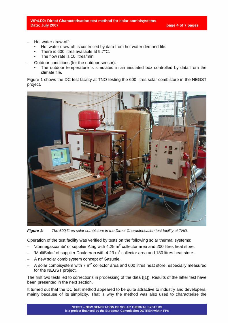
Figure 1 shows the DC test facility at TNO testing the 600 litres solar combistore in the NEGST project.

Figure 1: The 600 litres solar combistore in the Direct Characterisation test facility at TNO. Operation of the test facility was verified by tests on the following solar thermal systems: − ‘Zonnegascombi’ of supplier Atag with 4.25 m2 collector area and 200 litres heat store. − ‘MultiSolar’ of supplier Daalderop with 4.23 m2 collector area and 180 litres heat store. − A new solar combisystem concept of Gasunie. − A solar combisystem with 7 m2 collector area and 600 litres heat store, especially measured

for the NEGST project.

The first two tests led to corrections in processing of the data ([1]). Results of the latter test have been presented in the next section.

It turned out that the DC test method appeared to be quite attractive to industry and developers, mainly because of its simplicity. That is why the method was also used to characterise the




combination of solar domestic hot water system and gas-fired auxiliary heater as put together by suppliers Alpha Boilers and Itho Images. The method was even used as basis for characterising a conventional combisystem with gas saving device (Alpha Boilers) and a micro-system for cogeneration of heat and electricity (Gasunie). 2. DC TEST ON THE 600 LITRES COMBISTORE A full Direct Characterisation test has been carried out at TNO on a 600 litres solar combistore in combination with a common combi gas heater; see Figure 1. In the nine-days test, the solar combistore was combined with a simulated collector area of 7 m2. European climate zone II (Central European weather) was used for outdoor conditions and heat demand of the house was according to SFH100 with annual space heat demand of 51.27 GJ and hot water demand of 10.77 GJ. The nine-days test was carried out several times in order to also characterize and tune properties of the test facilities. The table below presents the results for two of the tests carried out. Table 1: DC test results and annual gas use as result of data processing for two the tests

on the 600 litres solar combistore.

Test QL,SH,test [GJ]

QL,dhw, test [GJ]

Vgas,test [m3]

mwater,test [kg]

Qcol,test [GJ]

Vgas,y [m3]

I 0.8896 0.1886 34.52 8.500 0.1185 2014 II 0.8897 0.1901 33.90 10.845 0.1682 1976

QL,SH,test: Heat delivered to space heating during the 6 days core phase of the test. QL,dhw, test: Heat delivered to hot water during the 6 days core phase of the test. Vgas,test: Gas used during the 6 days core phase of the test. mwater,test: Water mass from the combustion gas during the 6 days core phase of the test. Qcol,test: Collector output during the 6 days core phase of the test. Vgas,y: Annual gas use.

Conclusions from the test results in the table are: − The test facilities are able to reproduce conditions with respect to the loads very good: within

1%. − Gas use in the test differs due to difference in input from the collector. Of course this

difference can also be seen in the annual performance prediction.

Further research on the difference in collector input revealed a complex combination of grounds, i.e.: − Interaction between collector control and test facility behavior. − Sensitivity of collector control on ambient temperature as the store was not put up in a

conditioned room. − A non-optimized controller and solar combisystem.

Result was very frequent collector pump switching. Adaptation of the device of the test facility providing the heat from the collector led to less frequent collector switching and more unambiguous test results. 3. DC TESTING AND THE ENERGY PERFORMANCE OF BUILDINGS DIRECTIVE Recently, a new European standard, EN 15316-4-3 ([2]), on the thermal performance of solar domestic hot water (DHW) systems and solar combisystems was published. The new standard provides the link between European product standards and the Energy Performance of Buildings Directive (EPBD); see Figure 2. Product standards involve EN 12976-2 for solar DHW




systems, EN 12975-2 for solar collectors and EN 12977-3/4/5 for heat stores and controllers. EN 15316-4-3 supports two methods, i.e. the system approach and the component approach. For the component approach default values for collectors, heat stores and other components can be used to determine the thermal performance of the solar thermal system, or (better) values from component testing. Currently, the system approach has been elaborated for solar DHW systems only and uses the Dynamic System Test procedure as indicated in EN 12976-2. The DC test method provides a potential system approach for solar combisystems to be added in EN 15316-4-3 in future.

Figure 2: New European standard EN 15316-4-3 providing the link between product standards, the

DC test and the EPBD. New standard EN 15316-4-3 estimates reduction of heat load for any climate, space heating and hot water load (see Figure 3), whereas DC testing yields final energy use (and savings) of solar thermal for one climate, one space heating and one hot water load. That means that using the DC test result requires translation into EPBD terms. The so-called FSC method ([3]), result of the work in IEA Solar Heating and Cooling Task 26 may be used for this translation.

Figure 3: Input and output of European standard EN 15316-4-3. The FSC method presents the fractional energy savings Fsav as function of FSC. Fractional energy savings are obtained through dividing the savings by the final energy use of the reference system and the Fractional Solar Contribution presents the annual maximum contribution of solar energy to the final energy use of the reference system. This way of presentation enables characterisation of a solar combisystem in a single curve. Generally, every solar combisystems has its own curve; see Figure 4.




Figure 4: Exale of a calculated solar combisystem in various climates and houses presented in

energy savings as function of fractional solar contribution FSC (left) as well as a whole collection of solar combisystems presented in this way.

The slope of the curve in the FSC figure is rather constant for all solar combisystems. This provides the basis for extrapolation of the ‘one point’ DC result into thermal performance for a whole range of climates and heat demands; see Figure 5.

Figure 5: Example of extrapolation of the DC test result into thermal performance for a whole range

of climates and heat demands. REFERENCES [1] Visser, H. Solar combisystems – infrastructure for thermal performance

characterisation and possibilities for further knowledge development. Report no. 2004-DEG-R014, TNO, Delft, The Netherlands, 2004.

[2] Heating systems in buildings – Method for calculation of system energy requirements and system efficiencies – Part 4-3: Heat generation systems, thermal solar systems. European standard EN 15316-4-3, CEN, Brussels, Belgium.

[3] T. Letz. Validation and background information on the FSC procedure. Technical report Task 26 – Subtask A. IEA Solar Heating and Cooling Programme.

wp4.4. combi systems â€“ integrated or external boiler

Documents