worldline approach to the casimir effect
TRANSCRIPT

Worldline Approach to the Casimir Effect
Holger Gies
Institute for Theoretical PhysicsHeidelberg University
Holger Gies Worldline Approach to the Casimir Effect
”during my first years at Philips I did some workthat even Pauli regarded as physics ...
H.B.G. Casimir, Autobiography, 1983
Holger Gies Worldline Approach to the Casimir Effect

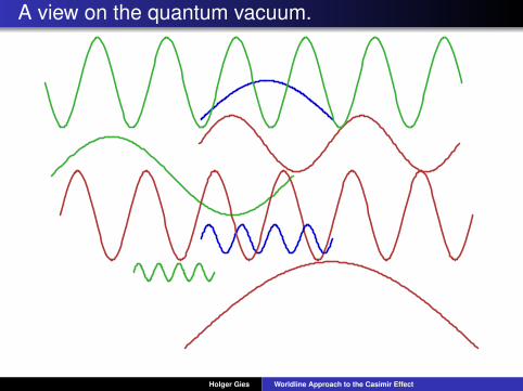
A view on the quantum vacuum.
Holger Gies Worldline Approach to the Casimir Effect
A view on the quantum vacuum.
Holger Gies Worldline Approach to the Casimir Effect

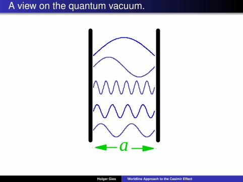
A view on the quantum vacuum.
Holger Gies Worldline Approach to the Casimir Effect

A view on the quantum vacuum.
Holger Gies Worldline Approach to the Casimir Effect
A view on the quantum vacuum.
a
Holger Gies Worldline Approach to the Casimir Effect

Casimir effect.
B origin:
E =12
∑~ω[a]− 1
2
∑~ω[∞]
B Hendrik B.G. Casimir 1948:
FA
= − π2
240~ ca4
relativistic: cquantum: ~“universal”: no other parameters
kgm · s2 =
kg ·m2
sms
1m4
Holger Gies Worldline Approach to the Casimir Effect

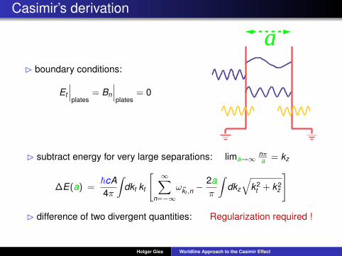
Casimir’s derivation
B boundary conditions:
Et
∣∣∣plates
= Bn
∣∣∣plates
= 0
a
B “vacuum energy”
12
∑~ω =
~2
A∫
d2kt
(2π)2
∞∑n=−∞
ω~kt ,n, ω~kt ,n
= c
√~k2
t +(πn
a
)2
Holger Gies Worldline Approach to the Casimir Effect

Casimir’s derivation
B boundary conditions:
Et
∣∣∣plates
= Bn
∣∣∣plates
= 0
a
B “vacuum energy”
12
∑~ω =
~2
A∫
d2kt
(2π)2
∞∑n=−∞
ω~kt ,n, ω~kt ,n
= c
√~k2
t +(πn
a
)2
→∞
Holger Gies Worldline Approach to the Casimir Effect
Casimir’s derivation
B boundary conditions:
Et
∣∣∣plates
= Bn
∣∣∣plates
= 0
a
B subtract energy for very large separations: lima→∞nπa = kz
∆E(a) =~cA4π
∫dkt kt
[ ∞∑n=−∞
ω~kt ,n− 2a
π
∫dkz
√k2
t + k2z
]
B difference of two divergent quantities: Regularization required !
Holger Gies Worldline Approach to the Casimir Effect

Casimir’s regulator
B smooth cutoff function F (k/km)
F (k/km) = 1 for k � km
F (k/km) = 0 for k →∞
“The physical meaning is obvious: for veryshort waves (X-rays, e.g.) our plate ishardly an obstacle at all and therefore thezero-points energy of these waves will notbe influenced by the position of the plate.”
Holger Gies Worldline Approach to the Casimir Effect

Casimir’s regulator
B smooth cutoff function F (k/km)
F (k/km) = 1 for k � km
F (k/km) = 0 for k →∞
B regularization~2
∑ω → ~
2
∑ω F (ω/km)
B remove the regulator
∆E(a) = limkm→∞
∆E reg(a) = −c~π2A720a3
Holger Gies Worldline Approach to the Casimir Effect

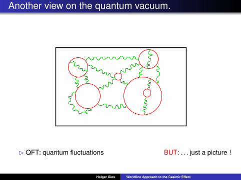
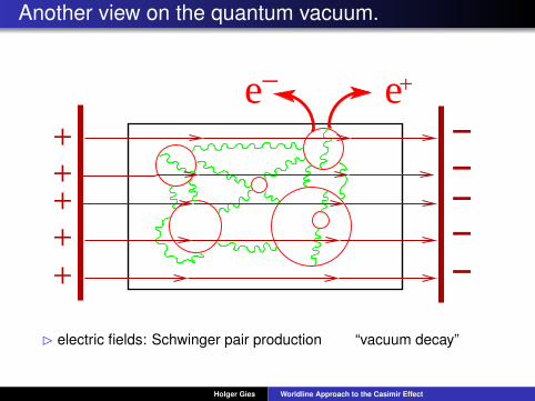
Another view on the quantum vacuum.
B ρ→ 0: “pneumatic vacuum”
Holger Gies Worldline Approach to the Casimir Effect
Another view on the quantum vacuum.
B QFT: quantum fluctuations BUT: . . . just a picture !
Holger Gies Worldline Approach to the Casimir Effect
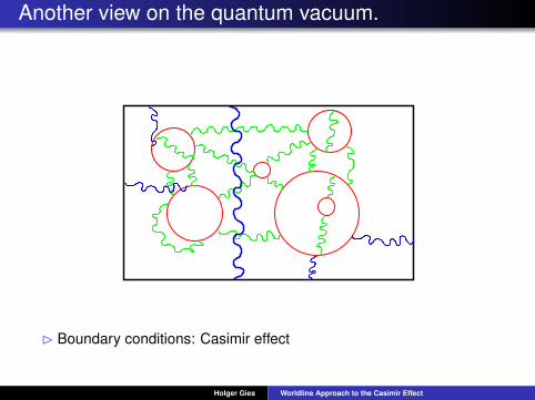
Another view on the quantum vacuum.
B Boundary conditions: Casimir effect
Holger Gies Worldline Approach to the Casimir Effect

Another view on the quantum vacuum.
B Probing the quantum vacuum, e.g., by external fields:“modified quantum vacuum”
Holger Gies Worldline Approach to the Casimir Effect
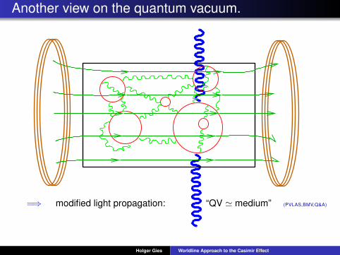
Another view on the quantum vacuum.
=⇒ modified light propagation: “QV ' medium” (PVLAS,BMV,Q&A)
Holger Gies Worldline Approach to the Casimir Effect
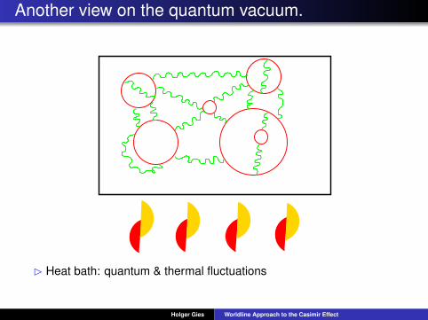
Another view on the quantum vacuum.
B Heat bath: quantum & thermal fluctuations
Holger Gies Worldline Approach to the Casimir Effect
Another view on the quantum vacuum.
+++++
−−−−−
ee + −
B electric fields: Schwinger pair production “vacuum decay”
Holger Gies Worldline Approach to the Casimir Effect

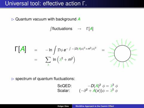
Universal tool: effective action Γ.
B Quantum vacuum with background A∫fluctuations → Γ[A]
Γ[A] =⇒
δΓ[A]δA = 0, quantum Maxwell equations → (light prop.)
EQV = Γ[A]T , FCasimir = −∂EQV
∂A , Casimir force
W = 2Im Γ[A]VT , Schwinger pair production rate
(HEISENBERG&EULER’36; WEISSKOPF’36; SCHWINGER’51)
(CASIMIR’48)
Holger Gies Worldline Approach to the Casimir Effect
Universal tool: effective action Γ.
B Quantum vacuum with background A∫fluctuations → Γ[A]
Γ[A] = − ln∫Dφe−
R−|D(A)φ|2+m2|φ|2 =
=∑
λ
ln(λ2 + m2
)
B spectrum of quantum fluctuations:
ScQED: −D(A)2 φ = λ2 φScalar: (−∂2 + A(x))φ = λ2 φ
Holger Gies Worldline Approach to the Casimir Effect

Universal tool: effective action Γ.
Γ[A] =∑
λ
ln(λ2 + m2
)=
Problem solved, “in principle”
find spectrum λ for a given background Asum over spectrum
Holger Gies Worldline Approach to the Casimir Effect
Universal tool: effective action Γ.
Holger Gies Worldline Approach to the Casimir Effect

Universal tool: effective action Γ.
Holger Gies Worldline Approach to the Casimir Effect

Universal tool: effective action Γ.
Γ[A] =∑
λ
ln(λ2 + m2
)=
BUT:
In general practice:
spectrum {λ} not knownanalyticallyspectrum {λ} not bounded∑
λ →∞ (regularization)renormalization
Holger Gies Worldline Approach to the Casimir Effect

Measurements of the Casimir force.
B Experimental milestones
Sparnaay 1958,van Blokland & Overbeek 1978,Lamoreaux 1997,Mohideen & Roy 1998,
∆FF ' 100%
∆FF ' 50%
∆FF ' 5%
∆FF ' 1%
B Sparnaay’s fundamental requirements:
clean plate surfacesprecise measurement of separation acontrol of electrostatic potentials Vres
Holger Gies Worldline Approach to the Casimir Effect
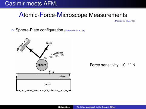
Casimir meets AFM.
Atomic-Force-Microscope Measurements(MOHIDEEN ET AL.’98)
B Sphere-Plate configuration (DERJAGUIN ET AL.’56)
Force sensitivity: 10−17 N
Holger Gies Worldline Approach to the Casimir Effect
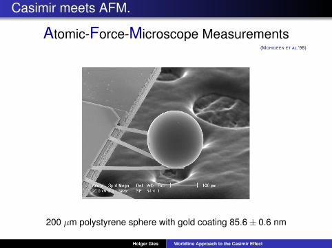
Casimir meets AFM.
Atomic-Force-Microscope Measurements(MOHIDEEN ET AL.’98)
200 µm polystyrene sphere with gold coating 85.6± 0.6 nm
Holger Gies Worldline Approach to the Casimir Effect

Casimir meets AFM.
Atomic-Force-Microscope Measurements(MOHIDEEN ET AL.’98)
B Sphere-Plate configuration (DERJAGUIN ET AL.’56)
B Results
B Corrections:
material
{surface roughness
finite conductivity
finite temperature
geometry
}QFT
Holger Gies Worldline Approach to the Casimir Effect

Casimir Morphology.(BINNS’05)
Holger Gies Worldline Approach to the Casimir Effect

Casimir Morphology.
a
R
F = − π2
240~ ca4 A F = ? F = ?
Holger Gies Worldline Approach to the Casimir Effect

Casimir vs. Newton.
B gravity:
F12 = − Gm1m2
|r1 − r2|2r12
B quantum force:
F‖ = − π2
240~ ca4 A
?Holger Gies Worldline Approach to the Casimir Effect

Casimir Edge Effects.
F‖ = − π2
240~ca4 · A
F1si = ?
(CF. BRESSI,CARUGNO,ONOFRIO,RUOSO’02)
Holger Gies Worldline Approach to the Casimir Effect

Casimir Edge Effects.
F‖ = − π2
240~ca4 · A
B parallel-plate
energy density
Holger Gies Worldline Approach to the Casimir Effect
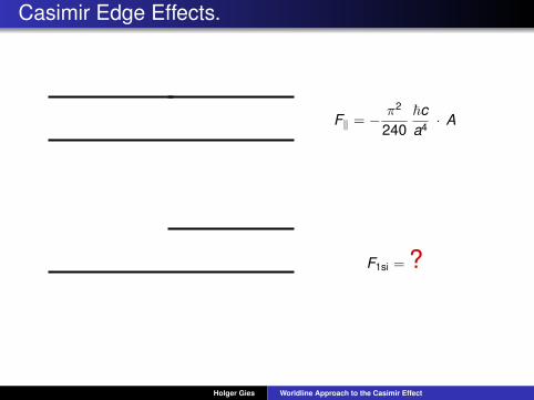
Casimir Edge Effects.
F‖ = − π2
240~ca4 · A
F1si = ?
Holger Gies Worldline Approach to the Casimir Effect

Casimir Edge Effects.
F‖ = − π2
240~ca4 · A
F1si = ?
Holger Gies Worldline Approach to the Casimir Effect

Casimir Edge Effects.
F‖ = − π2
240~ca4 · A
F1si = ?
Holger Gies Worldline Approach to the Casimir Effect

Worldline representation of Γ.
B pedestrian approach
Γ[A] =∑
λ
ln(λ2 + m2
)= Tr ln
[−(D(A))2 + m2
]
= −∞∫
1/Λ2
dTT
e−m2T Tr exp[D(A)2 T
]︸ ︷︷ ︸
=〈x|eiH(iT )|x〉
= −∞∫
1/Λ2
dTT
e−m2T N∫
x(T )=x(0)
Dx(τ) e−
TR0
dτ“
x24 +ie x·A(x(τ)
”
Holger Gies Worldline Approach to the Casimir Effect
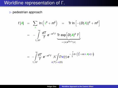
Worldline representation of Γ.
B pedestrian approach
Γ[A] =∑
λ
ln(λ2 + m2
)= Tr ln
[−(D(A))2 + m2
]
= −∞∫
1/Λ2
dTT
e−m2T Tr exp[D(A)2 T
]︸ ︷︷ ︸
=〈x|eiH(iT )|x〉
= −∞∫
1/Λ2
dTT
e−m2T N∫
x(T )=x(0)
Dx(τ) e−
TR0
dτ“
x24 +ie x·A(x(τ)
”
Holger Gies Worldline Approach to the Casimir Effect

Worldline representation of Γ.
Γ[A] = −∞∫
1/Λ2
dTT
e−m2T N∫
x(T )=x(0)
Dx(τ) e−
TR0
dτ“
x24 +ie x·A(xτ)
”
x(T ) =
(FEYNMAN’50)
...(HALPERN&SIEGEL’77)
(POLYAKOV’87)
(FERNANDEZ,FRÖHLICH,SOKAL’92)
...(BERN&KOSOWER’92; STRASSLER’92)
(SCHMIDT&SCHUBERT’93)
(KLEINERT’94)
Holger Gies Worldline Approach to the Casimir Effect

Worldline representation of Γ.
Γ[A] = −∞∫
1/Λ2
dTT
e−m2T N∫
x(T )=x(0)
Dx(τ) e−
TR0
dτ“
x24 +ie x·A(xτ)
”
x(T ) =
Worldline approach:
effective action Γ ∼∫
closed worldlines x(τ)
worldline ∼ spacetime trajectory of φ fluctuationsgauge-field interaction ∼ “Wegner-Wilson loop”finding {λ} and
∑λ done in one finite (numerical) step (HG&LANGFELD’01)
Holger Gies Worldline Approach to the Casimir Effect

Worldline Numerics.
∫x(1)=x(0)
Dx(t) −→nL∑
l=1
, nL = # of worldlines
→ statistical error
x(t) −→ x i , i = 1, . . . ,N (ppl)→ systematical error
−→ → spacetime remains continuous
Holger Gies Worldline Approach to the Casimir Effect

Trajectory of a Quantum Fluctuation.
B Feynman diagram (conventionally in momentum space)
Holger Gies Worldline Approach to the Casimir Effect

Trajectory of a Quantum Fluctuation.
B worldline (artist’s view)
Holger Gies Worldline Approach to the Casimir Effect

Trajectory of a Quantum Fluctuation.
B worldline numerics: N = 4 points per loop (ppl)
Holger Gies Worldline Approach to the Casimir Effect

Trajectory of a Quantum Fluctuation.
B worldline numerics: N = 10 points per loop (ppl)
Holger Gies Worldline Approach to the Casimir Effect

Trajectory of a Quantum Fluctuation.
B worldline numerics: N = 40 points per loop (ppl)
Holger Gies Worldline Approach to the Casimir Effect

Trajectory of a Quantum Fluctuation.
B worldline numerics: N = 100 points per loop (ppl)
Holger Gies Worldline Approach to the Casimir Effect
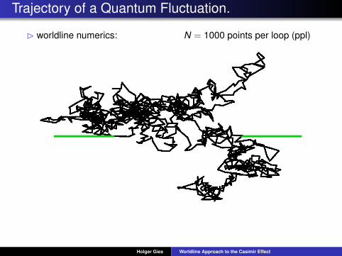
Trajectory of a Quantum Fluctuation.
B worldline numerics: N = 1000 points per loop (ppl)
Holger Gies Worldline Approach to the Casimir Effect

Trajectory of a Quantum Fluctuation.
B worldline numerics: N = 10000 points per loop (ppl)
Holger Gies Worldline Approach to the Casimir Effect

Trajectory of a Quantum Fluctuation.
B worldline numerics: N = 100000 points per loop (ppl)
Holger Gies Worldline Approach to the Casimir Effect

Propertime T .
T ∼ regulator scale of smeared momentum shells
Holger Gies Worldline Approach to the Casimir Effect

Propertime T .
B “Measuring” the Wegner-Wilson loop exp(−ie
∮dx · A
)
Holger Gies Worldline Approach to the Casimir Effect

Casimir Effect.
B Casimir effect = “strong-field QFT”
S =12
(∂φ)2 +m2
2φ2 + Aφ2
A(x) = λ
∫S
dσ[δ(x − xσ) + δ(x − xσ)
]
xσ
xσ
(BORDAG,HENNIG,ROBASCHIK’92; GRAHAM ET AL.’03)
B Casimir energy on the worldline:
E [A] = −12
∞∫0
dTT
e−m2T N∫
x(T )=x(0)
Dx(τ) e−
TR0
dτ“
x24 +A(x(τ))
”
Holger Gies Worldline Approach to the Casimir Effect

Benchmark test: parallel plates
Holger Gies Worldline Approach to the Casimir Effect

Benchmark test: parallel plates
Holger Gies Worldline Approach to the Casimir Effect

Benchmark test: parallel plates
B for finite m, λ, a
(BORDAG,HENNIG, ROBASCHIK ’92) (HG,LANGFELD,MOYAERTS ’03)
Holger Gies Worldline Approach to the Casimir Effect

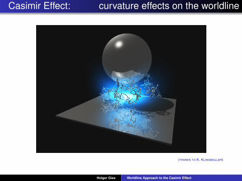
Casimir Effect: curvature effects on the worldline
S2
(a) (b) (c)
S1
Holger Gies Worldline Approach to the Casimir Effect

Casimir Effect: curvature effects on the worldline
−εR
4
0.012
0.01
0.008
0.006
0.004
0.002
0
Holger Gies Worldline Approach to the Casimir Effect
Casimir Effect: curvature effects on the worldline
(THANKS TO K. KLINGMULLER)
Holger Gies Worldline Approach to the Casimir Effect

Casimir Effect: sphere above plate.
0.001 0.01 0.1 1 10 100a/R
0
0.5
1
1.5
2
EC
asim
ir/E
PFA
(a/R
<<
1)
PFA plate-basedPFA sphere-based
Holger Gies Worldline Approach to the Casimir Effect

Casimir Effect: sphere above plate.
0.001 0.01 0.1 1 10 100a/R
0
0.5
1
1.5
2E
Cas
imir/E
PFA
(a/R
<<
1)
PFA plate-basedPFA sphere-basedworldline numerics
Holger Gies Worldline Approach to the Casimir Effect

Casimir Effect: sphere above plate.
0.001 0.01 0.1 1 10 100a/R
0
0.5
1
1.5
2E
Cas
imir/E
PFA
(a/R
<<
1)
PFA plate-basedPFA sphere-basedoptical approximationworldline numerics"KKR" multi-scattering map
(HG,LANGFELD,MOYAERTS’03; JAFFE,SCARDICCHIO’04; BULGAC,MAGIERSKI,WIRZBA’05; HG,KLINGMÜLLER’05)
Holger Gies Worldline Approach to the Casimir Effect

Future Casimir curvature measurements.
B cylinder-plate geometry (BROWN-HAYES,DALVIT,MAZZITELLI,KIM,ONOFRIO’05)
(EMIG,JAFFE,KARDAR,SCARDICCHIO’06; HG,KLINGMULLER’06; BORDAG’06)
Holger Gies Worldline Approach to the Casimir Effect

Casimir Edge Effects.
F‖ = −γ‖~ca4 · A
F1si = ?
(CF. BRESSI,CARUGNO,ONOFRIO,RUOSO’02)
Holger Gies Worldline Approach to the Casimir Effect

Casimir Edge Effects.
F‖ = −γ‖~ca4 · A
F1si = ?
(CF. BRESSI,CARUGNO,ONOFRIO,RUOSO’02)
Holger Gies Worldline Approach to the Casimir Effect

Casimir Edge Effects.
F‖ = −γ‖~ca4 · A
F1si = ?
(CF. BRESSI,CARUGNO,ONOFRIO,RUOSO’02)
Holger Gies Worldline Approach to the Casimir Effect

Casimir Edge Effects.
Σ2
aΣ1
Holger Gies Worldline Approach to the Casimir Effect

Casimir Edge Effects.
εC
asim
ira
4
0
-0.002
-0.004
-0.006
-0.008
-0.01
-0.012
-0.014
Holger Gies Worldline Approach to the Casimir Effect
Casimir Edge Effects.
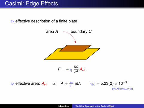
B effective description of a finite plate
area A boundary C
F = −γ‖~ca4 Aeff,
B effective area: Aeff ' A + γ1siγ‖
aC, γ1si = 5.23(2)× 10−3
(HG,KLINGMULLER’06)
Holger Gies Worldline Approach to the Casimir Effect

Casimir Edge Effects.
B effective description of a finite plate
area A boundary C
F = −γ‖~ca4 Aeff,
B effective area: Aeff ' A + γ1siγ‖
aC, γ1si = 5.23(2)× 10−3
(HG,KLINGMULLER’06)
Holger Gies Worldline Approach to the Casimir Effect

Further Worldline Applications.
Heisenberg-Euler effective actions, spinor QED,flux tubes, quantum-induced vortex interactions
(HG,LANGFELD’01; LANGFELD,MOYAERTS,HG’02)
thermal fluctuations, free energies(HG,LANGFELD’02)
+++++
−−−−−
ee + − “spontaneous vacuum decay”, Schwinger pairproduction in inhomogeneous electric fields
(HG,KLINGMÜLLER’05)
nonperturbative effective actions(HG,SÁNCHEZ–GUILLÉN,VÁZQUEZ’05)
Holger Gies Worldline Approach to the Casimir Effect

Higher loops per pedes
B Feynman diagrammar:
∼∫
dDp1
(2π)D
∫dDp2
(2π)D
∏i
∆i(qi)
Holger Gies Worldline Approach to the Casimir Effect

Higher loops per pedes
B Worldline:
∼∫
T
⟨ ∫dτ1dτ2 ∆(x(τ1), x(τ2))
⟩x
B photon propagator in coordinate space
∆(x1, x2) =
∫dDp
(2π)D1p2 eip(x1−x2) =
Γ(D−2
2
)4πD/2
1|x1 − x2|D−2
Holger Gies Worldline Approach to the Casimir Effect

Higher loops per pedes
B Worldline:
∼∫
T
⟨e−ie
Hdx·A(x)
∫dτ1dτ2 ∆(x(τ1), x(τ2))
⟩x
Holger Gies Worldline Approach to the Casimir Effect

Higher loops per pedes
B Feynman diagrammar:
+ ∼∫
dDp1
(2π)D
∫dDp2
(2π)D
∫dDp3
(2π)D
∏i
∆i(qi)
+
∫dDp1
(2π)D
∫dDp2
(2π)D
∫dDp3
(2π)D
∏i
∆i(qi)
Holger Gies Worldline Approach to the Casimir Effect
Higher loops per pedes
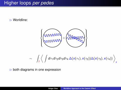
B Worldline:
+
∼∫
T
⟨ ∫dτ1dτ2dτ3dτ4 ∆(x(τ1), x(τ2))∆(x(τ3), x(τ4))
⟩x
B both diagrams in one expression
Holger Gies Worldline Approach to the Casimir Effect

Higher loops per pedes
B Worldline:
+
∼∫
T
⟨ (∫dτ1dτ2 ∆(x(τ1), x(τ2))
)2 ⟩x
B both diagrams in one expression
Holger Gies Worldline Approach to the Casimir Effect
Higher loops per pedes
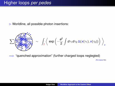
B Worldline, all possible photon insertions:
∑∼
∫T
⟨exp
(−e2
2
∫dτ1dτ2 ∆(x(τ1), x(τ2))
) ⟩x
=⇒ “quenched approximation” (further charged loops neglegted)(FEYNMAN’50)
Holger Gies Worldline Approach to the Casimir Effect
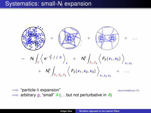
Systematics: small-Nf expansion
+ + + . . .
∼ Nf
∫T
⟨e−
e22
R R∆
⟩x
+ N2f
∫T 1,T 2
⟨F2{x1, x2}
⟩x1,x2
+ N3f
∫T 1,T 2,T 3
⟨F3{x1, x2, x3}
⟩x1,x2,x3
+ . . .
=⇒ “particle-~ expansion” (HALPERN&SIEGEL’77)
=⇒ arbitrary g, “small” A (. . . but not perturbative in A)
Holger Gies Worldline Approach to the Casimir Effect
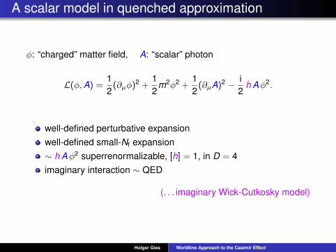
A scalar model in quenched approximation
φ: “charged” matter field, A: “scalar” photon
L(φ,A) =12
(∂µφ)2 +12
m2φ2 +12
(∂µA)2 − i2
h Aφ2.
well-defined perturbative expansionwell-defined small-Nf expansion∼ h Aφ2 superrenormalizable, [h] = 1, in D = 4imaginary interaction ∼ QED
(. . . imaginary Wick-Cutkosky model)
Holger Gies Worldline Approach to the Casimir Effect
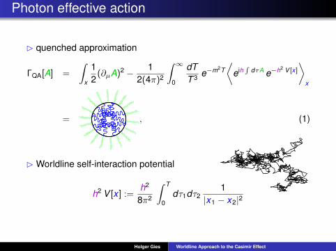
Photon effective action
B quenched approximation
ΓQA[A] =
∫x
12
(∂µA)2 − 12(4π)2
∫ ∞
0
dTT 3 e−m2T
⟨eih
RdτA e−h2 V [x ]
⟩x
= , (1)
B Worldline self-interaction potential
h2 V [x ] :=h2
8π2
∫ T
0dτ1dτ2
1|x1 − x2|2
Holger Gies Worldline Approach to the Casimir Effect

Self-interaction potential
Holger Gies Worldline Approach to the Casimir Effect

Self-interaction potential
Holger Gies Worldline Approach to the Casimir Effect
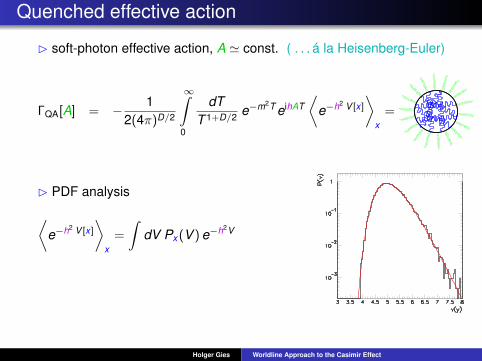
Quenched effective action
B soft-photon effective action, A ' const. ( . . . á la Heisenberg-Euler)
ΓQA[A] = − 12(4π)D/2
∞∫0
dTT 1+D/2 e−m2T eihAT
⟨e−h2 V [x ]
⟩x
=
B PDF analysis⟨e−h2 V [x ]
⟩x
=
∫dV Px(V ) e−h2V
Holger Gies Worldline Approach to the Casimir Effect
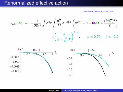
Renormalized effective action(HG,SANCHEZ-GUILLEN,VAZQUEZ’05)
ΓQA,R[A] = − 132π2
∫d4x
∞∫0
dTT 3 e−m2
RT(
eihAT − 1− ihAT +(hAT )2
2
)
×
(β
β + h2
8π2 T
)1+α
, α ' 0.79, β ' 13.2
0.5 1 1.5 2A
-0.002
-0.0015
-0.001
-0.0005
Re G 8h=1<
0.5 1 1.5 2A
-0.8
-0.6
-0.4
-0.2
Re G 8h=5<
Holger Gies Worldline Approach to the Casimir Effect

Massless Limit?
B one-loop small-φ-mass limit: IR divergence
Γ1-loop[A]∣∣
hAm2
R�1 ' −
164π2
∫d4x (hA)2 ln
hAm2
R
B quenched small-φ-mass limit: finite
ΓQA,R[A]|mR=0 = −[−Γ(−2− α)] cos π
2α
25−3απ2(1−α)βα
∫d4x (hA)2
(Ah
)α
[1+O((A/h))]
=⇒ break-down of massless limit ∼ artifact of perturbation theory
. . . large log’s summable
Holger Gies Worldline Approach to the Casimir Effect

Conclusions.
Probing the quantum vacuum by strongfields, Casimir boundaries, etc . . .
. . . brings QFT to the desktop
“quantum fields meet micro mechanics”
Worldline numerics :
efficient tool
intuitive picture
Holger Gies Worldline Approach to the Casimir Effect

Conclusions.
Probing the quantum vacuum by strongfields, Casimir boundaries, etc . . .
. . . brings QFT to the desktop
“quantum fields meet micro mechanics”
Worldline numerics :
efficient tool
intuitive picture
Holger Gies Worldline Approach to the Casimir Effect

Conclusions.
Probing the quantum vacuum by strongfields, Casimir boundaries, etc . . .
. . . brings QFT to the desktop
“quantum fields meet micro mechanics”
Worldline numerics :
efficient tool
intuitive picture
Holger Gies Worldline Approach to the Casimir Effect

Holger Gies Worldline Approach to the Casimir Effect

Fermions on the worldline I.
B Grassmann loops
Γ1spin = ln det
[γµ∂µ + ieγµAµ + m
]= − 1
2(4π)D/2
∫ ∞
1/Λ2
dTT 1+D/2 e−m2T
∫PDx∫
ADψ e−
R T0 dτLspin
Lspin =14
x2 + iexµAµ+12ψµψ
µ − ieψµFµνψν
Holger Gies Worldline Approach to the Casimir Effect

Fermions on the worldline II.
B spinor QED (parity-even part):
Γ =− 1
2
(4π)D2
∫dDxCM
∞∫1/Λ2
dTT D
2 +1e−m2T
⟨Wspin[A]
⟩x
Wspin[A] = W [A] × PT exp
ie2
T∫0
dτ σµνFµν
Fσ Fσ
FσFσ
FσFσFσ
FσFσ
Fσ
FσFσ
Holger Gies Worldline Approach to the Casimir Effect
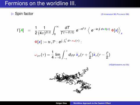
Fermions on the worldline III.
B Spin factor (STROMINGER’80,POLYAKOV’88)
Γ[A] =12
1(4π)D/2
∫ ∞
0
dTT (1+D/2)
e−m2T⟨
e−ieH
dxA(x) Φ[x ]⟩
x
Φ[x ] := trγP : ei2
R T0 dτ σω(τ) :
ωµν(τ) =14
limε→0
∫ ε
−ε
dρρ xµ(τ +ρ
2)xν(τ − ρ
2)
(HG&HAMMERLING’05)
Holger Gies Worldline Approach to the Casimir Effect