world bank human development network health, nutrition and...

1

World Bank Human Development Network

Health, Nutrition and Population Unit

Results-Based Financing for Health Impact Evaluation

Handbook For Data Analysts

In Impact Evaluations

Part I: Baseline Household

Data Analysis

2

CONTENTS

ABBREVIATIONS AND ACRONYMS ................................................................................................ 3

INTRODUCTION ............................................................................................................................ 4

1 GENERAL DO’S AND DON’TS ................................................................................................... 7

1.1 DATA ASSESSMENT .................................................................................................................. 7 1.2 DATA CLEANING ..................................................................................................................... 9 1.3 MERGING DATASETS .............................................................................................................. 10 1.4 CONSTRUCTING NEW VARIABLES .............................................................................................. 11 1.5 DATA ANALYSIS .................................................................................................................... 13

2 VALIDATING EVALUATION DESIGN........................................................................................ 14

2.1 UNDERSTANDING STUDY ARMS ................................................................................................ 14 2.2 CLUSTERING AND WEIGHTING, SURVEY OR “SVY” DATASET ............................................................. 16 2.3 INITIAL ANALYSIS ON “SVY” AND NON “SVY” DATA ........................................................................ 17 2.3.1 CALCULATING MEANS FOR THE TOTAL SAMPLE .................................................................................... 18 2.3.2 CALCULATING MEANS FOR EACH STUDY ARM ...................................................................................... 18 2.3.3 DIFFERENCE IN MEANS TESTS ACROSS STUDY ARMS ............................................................................. 18 2.3.4 USING THE F-TEST OF DIFFERENCE IN MEANS ...................................................................................... 22

3 CONSTRUCTING KEY HOUSEHOLD AND INDIVIDUAL OUTPUTS AND OUTCOMES .................... 23

4 GENERATING COVARIATE VARIABLES FROM THE HOUSEHOLD SURVEY ................................. 23

3

Abbreviations and acronyms

ANC: Antenatal care CHW: Community Health Workers DHS: Demographic and Health Surveys GOR: Government of Rwanda HNP: Health Nutrition and Population ID: Identifier IE: Impact Evaluation JHU: Johns Hopkins University PBF: Performance-Based Financing RBF: Results-Based Financing WHO: World Health Organization

4

Introduction

This handbook intends to guide data analysts supporting the impact evaluation of Results-Based Financing (RBF) for health programs. The Global IE team that supports evaluation in the context of the Health Results Innovation Trust Fund developed it.

Goal of the handbook

This handbook presents techniques and tips that data analysts can use to:

Clean and analyze baseline household data using STATA software version 10 SE,

Produce a baseline household report that assesses the difference in means between treatment and comparison groups at baseline and calculates outcome indicators.

Companion resources

Data analysts can find additional supporting materials referenced in the Impact Evaluation Toolkit developed by the Global IE team, and posted on the Analysis tab of the RBF impact evaluation website http://hrbfevaluation.org. A few additional resources are also available under the Workshop tab of the http://hrbfevaluation.org website. This handbook will refer to these resources, listed in table 1, whenever data analysts should consult them.

The examples given throughout this handbook are based on the 2010 Rwanda Community Performance-Based Financing (PBF) impact evaluation baseline data.

Handbook structure

This handbook is structured as follows:

Section 1: General Do’s and Don’ts. This section reviews the main guidelines to get started with data analysis on STATA software

Section 2: Validating evaluation design. This section explains study arms assignment, how to set up the dataset, calculate means and run mean tests across treatment groups on STATA software

Section 3: Constructing key household and individual outcomes and outputs. This section provides an overall guide to create indicators appropriately.

Section 4: Generating covariate variables from the household survey. This section highlights the general technique data analysts should use to create covariates

5

Table 1: Resources for Data Analysis

Tasks Instruments Where to find instruments Reproducibility of instruments

Create outcome and output indicators

Create general variables and core output and outcome indicators

Johns Hopkins University (JHU) report on core indicators to be calculated to assess program impact: lists inputs/ process/ outputs/ outcome/ impact indicators that could be calculated to evaluate an RBF intervention

Referenced in Toolkit, Chapter 7: Data Analysis & Dissemination. Posted at http://hrbfevaluation.org

Reference only

World Health Organization (WHO) Indicators Compendium 2010

http://www.who.int/gho/indicator_registry/en/

Reference only

Table of core indicators calculated for the analysis of RBF in Rwanda based on JHU and WHO guidelines, with corresponding STATA codes (to be used as reference but each IE should develop its own depending on their indicators)

Toolkit, Chapter 7: Data Analysis & Dissemination Posted at http://hrbfevaluation.org

Serves as reference for definition of indicators on STATA, but data analyst should develop its own table according to indicators relevant to country analysis

Do-files developed on Rwanda RBF analysis cleaning data, creating variables and output/outcome indicators for mean tests: do-files starting with “rwanda_cr” from “rwanda_cr1” to “rwanda_cr27”


Serves as reference for STATA codes, but data analyst should develop own codes for cleaning and creation of variables according to relevance for country study

Conduct data analysis including mean tests and graphs

Calculate means, for treatment groups altogether and by treatment group. Perform mean tests

Do-files developed for the Rwanda RBF analysis of baseline data: do-files starting with “rwanda_an” from “rwanda_an2” to “rwanda_an5” + “rwanda_an1000_programs” which defines programs calculating means, running mean tests and saving results. Ado-file “iesummarystats” and “svyiesummarystats” performing mean tests and creating standardized tables of results. Should be loaded into STATA personal ado-file folder.


Do-files serve as reference for STATA codes but should be tailored to analysis of country-specific variable names. Do-file “rwanda_an1000_programs” and ado-file “iesummarystats” and “svyiesummarystats” may be used as is and facilitate reproducibility of results

Produce standardized Do-files compiling all results obtained from Rwanda Toolkit, Chapter 7: Data Analysis & Do-files should be tailored to

6

Tasks Instruments Where to find instruments Reproducibility of instruments

tables of those results RBF analysis in standardized tables: do-files “rwanda_cr28”. “rwanda_cr29”, “rwanda_cr30”

Dissemination Posted at http://hrbfevaluation.org

country-specific variable names and dataset names

Create additional tables on sample structure and % of unbalanced variables

Do-files “rwanda_an1”, “rwanda_cr31”, “rwanda_an7” and “rwanda_an8”


Do-files serve as reference for STATA codes and potential content. Should be tailored to country analysis

Graph relevant indicators and variables

Do-file “rwanda_an6_graphs” Toolkit, Chapter 7: Data Analysis & Dissemination Posted at http://hrbfevaluation.org

Reference for STATA codes and graph techniques. Variable names should be adjusted.

Obtain general support for data analysis and specific commands

PowerPoint presenting commands and methodology to obtain tables assessing sample balance across treatment groups

Workshops, Tunis 2010, STATA Lesson 3 Posted at http://hrbfevaluation.org

Reference only

Other PowerPoints giving general STATA commands, including graphs commands

Workshops, Tunis 2010, STATA Lessons 1 and 2 Posted at http://hrbfevaluation.org

Reference only

General guide to main STATA commands Workhops, Tunis 2010, STATA Getting Started Guide Posted at http://hrbfevaluation.org

Reference only

STATA Lessons materials including problem sets Workhops, Tunis 2010, STATA Lessons materials Posted at http://hrbfevaluation.org

Reference only

Disseminate results in report

Write report 2010 Rwanda baseline survey analysis report Toolkit, Chapter 7: Data Analysis & Dissemination Posted at http://hrbfevaluation.org

Reference on structure and content of the report.

Source: Author

7

1 General do’s and don’ts

We start with a review of a few general recommendations for data analysts to consider prior to initiating data analysis.

1.1 Data Assessment

Never modify the original datasets. Make sure you don’t risk altering the original data, by saving the datasets under a new name, or in a different directory. Before starting the analysis, create a “data” folder, with the following subfolders: “original”, “clean”, “temp”. When opening an original dataset from the “original” folder, never save it back to the same location, but in the “clean” or “temp” folder.

Work in STATA do-files. STATA do-files offer two advantages: (i) replicating results and (ii) improving efficiency for future analysis.

A very important element of data analysis is being able to replicate results. Since many of the variables required for analysis necessitate construction across multiple variables in the original databases, a STATA do file serves as the dictionary for how variables are constructed, as well as how difference in means tests are specified and exported.

Do-files also allow you to work more efficiently. STATA codes developed for baseline data analysis will be useful as a basis to develop codes for the analysis of follow-up and endline surveys, since variable names should be the same across survey rounds. For example the definition of indicators on do-files can be reused at endline to calculate the value of those indicators at endline.

Define a directory do-file

Reference Do-files:

rwanda_directories

A directory do-file uses macros to define the path to the “data”, “dofiles”, “logfiles” and “results” folders, or directories. When you run the directory do-file, STATA defines a macro for each of these directories. In the do-files that you run subsequently to the directory do-file, every time STATA needs to access these folders, you can use these macros instead of having to write out file paths, which can save a lot of time. In addition, if you wish to run the same analysis on another computer where file paths may be different, you will only need to modify the directories do-file, and not all of your do-files.

Define a master do-file

Reference Do-files:

rwanda_master

The master do-file indicates in which order do-files should be run, and briefly describes what each do-file does. The master do-file is the first point of entry for anyone who wants an overview of the data analysis. Data analysts will find that a master do-file helps them return to the analysis more easily after breaks in the analysis.

In the Rwanda community PBF example, do-files listed in the master do-file starting with “rwanda_cr” create new datasets or variables (“cr” standing for create). Do-files starting with “rwanda_an” conduct the analysis (“an” standing for analysis).

8

Label datasets with one word. In STATA, using quotes is sometimes cumbersome, and can create difficulties if combined with the name of a macro. If the name of your dataset is not in one word, you will have to use quotes every time you refer to the dataset, and you may experience difficulties assigning macros. To avoid this issue, just rename your original dataset and name any new datasets in one word, using underscore as a separation if needed.

Identify critical variables in your datasets. Prior to data analysis, you should be able to correctly identify the key variables in the datasets:

Study arm: confirm the appropriate variable for defining assignment to treatment group (or groups) and comparison group.

Unit of assignment: Following the sampling plan, the cluster unit should be clearly identified in the documentation and data.

Weights: Following the sampling plan, you may need to weight the data for it to be representative of the target population. If weights do not exist already, you may have to create weights yourself. During sampling, a mapping of the households present in each geographic entity, or the number of districts, sectors, etc. per geographic entity, must have been created. Refer to this documentation to calculate weights appropriately.

Unique Identifiers (IDs): Spot household and individual unique identifiers. They are usually the key variables allowing you to merge the different sections of the datasets together. When defined correctly - and this is something to check absolutely, they uniquely identify an individual, or a household.

Understand the level of your datasets. RBF datasets can feature information on households, household members, health facilities, Community Health Workers (CHWs), CHW cooperatives, etc. In the RBF household data, datasets can be at the health sector level, household level, or individual level. A sector-level dataset includes one observation for each sector, a household-level dataset one observation for each household, and an individual-level dataset one observation for each participant in the survey (or each respondent in a given section of the questionnaire). Some datasets from the household survey are even defined at a sub-individual level, as explained in the examples below.

Reference Do-files:

rwanda_cr1_a00

rwanda_cr10_a06

rwanda_cr18_b06

Based on the construction of the RBF household Data Entry Program, most datasets are at the individual level, i.e. one row corresponds to one individual. However, other datasets are presented differently, and you should browse or codebook your dataset to figure out which level you will be working on and if any changes are necessary. For example:

Dataset A00 (or RWHRBF_A_HOUSEHOLD-00.dta) is at the household level: one observation corresponds to one household.

Dataset A06 (or RWHRBF_A_HOUSEHOLD-06.dta) is at the livestock level: for each household, there are 9 rows that correspond to the 9 kinds of livestock the household may own (1-Cattle, 2-Goat, 3-Sheep, etc.). We created new variables and reformatted the data to obtain household-level statistics.

Dataset B06 (or RWHRBF_B_FEMALE-06.dta) is at the pregnancy-level: for each woman, the dataset contains one row per pregnancy that took place since January 2008. Depending on the number of pregnancies that a woman had, the number of rows per woman thus varies.

Investigate when something looks wrong. Review the data for any immediate anomalies before initiating data construction or analysis. Carefully review key variables, such as unique identifiers, key administrative level variables or study arm variables, for any missing or repeated values. The survey

9

team and survey firm reports may be able to justify any missing data, however you should also correct repeated observations prior to data analysis.

Keep a record and document any recurring error and discuss it with the survey team.

1.2 Data Cleaning

All of the recommendations below refer to do-files developed to create databases for analysis, i.e. do-files that should start with the “country_cr” prefix.

Make sure that unique identifiers are unique. In Chapter 6 of the RBF for Health Impact Evaluation Toolkit, we explain how the IE team and survey firm can uniquely identify observations within the dataset(s) using geo-codes as well as RBF specific unique identification codes.

Once the dataset(s) is (are) produced, it is your turn to confirm whether each observation is uniquely identified. In STATA, the commands duplicates report or duplicates tag report whether there are any ID duplicates in the dataset.

Please note: Do not create a new variable combining household and individual identifiers. Say you have household number 12, and individual number 14, and household number 121, and individual number 4. Both combinations of household and individual IDs give the same number, 1214, so you would create duplicates. Please check Chapter 6 of the RBF for Health Impact Evaluation Toolkit for recommendations on how to create a unique identifier that is linked to the geo-codes.

Check and correct the range of variables. You will need to systematically check the range of all variables, and correct out-of-range values. Where values cannot be corrected, you should reassign out-of-range values to missing values. STATA provides not only standard missing values represented by a dot in STATA, but also missing values represented by a dot followed by a letter (.a, .b. …, .z). These letters can replace out-of-range values if you wish to distinguish which observations were originally missing and which ones were out of range. If you do so, please remember that a non-missing value will be different from a dot missing value and different from a letter missing value, therefore it will be “<.” but not only “!=.”(see help missing in STATA for more details).

In the “rwanda_cr” do-files, we tabulated all variables using the tab1 command to assess variables range. Another command that could be used to make sure no variable equals absurd values is assert.

Confirm skips between questions are respected. It happens that during the interview, enumerators forget to skip some questions if the respondent answered in a specific way to the previous question. Again assert is a useful command to make sure skips are respected: you can assert a variable that should have been skipped in certain conditions is indeed missing under these conditions.

Confirm respondents” answers are logical with respect to previous answers. A good way to check data quality is to cross-check answers with one another when a logical link exists between questions. You can use the assert command for that. You can also cross-tabulate two variables in order to check respondents” answers are consistent, using tabulate (twoway).

Reference Do-files:

rwanda_cr18_b06

To verify the accuracy of the skilled delivery indicator, we cross-tabulate variables b13_058 and b13_059, which assess respectively who assisted with the delivery and in which kind of facility the woman delivered. The majority of women who indicated a skilled delivery should have delivered in a formal health facility, even if skilled professionals may have assisted a minority of women in a different place, at home for example. In-country health specialists should be able to inform you on what should or should not occur in the

10

country context.

1.3 Merging Datasets

Correctly merging datasets is essential to a correct analysis, but it can be a tricky exercise. Here are a few tips to help you merge your data successfully.

Identify which variable(s) should be used as the merging variable to merge datasets. Sometimes, it may not be obvious what variable(s) should be used to merge two or more datasets. Be sure you identify whether you need to merge on one or more variables. For example, if you want to merge two individual-level datasets, you will need to merge based on complete individual unique identifiers.

Reference Do-files:

rwanda_cr3_a02

rwanda_cr23_c01

In the Rwanda Community PBF household datasets, individual IDs are composed of the combination of a health sector ID variable (hrbf_id1), a household ID variable (hrbf_id2), and a household member ID (generally renamed as a1_pid). To merge the roster of all individuals in each household with each individual-level dataset, such as the education section dataset A02 (or RWHRBF_A_HOUSEHOLD-02), all those three variables have to be matched and used as the merging variables. For the merge to work, each combination of hrbf_id1/hrbf_id2/a1_pid has to be unique in each dataset, and the data have to be sorted according to these variables prior to or during the merge. We use the following commands after the data have been sorted:

use $cleandatadir/rwhrbf_household_roster.dta, clear merge hrbf_id1 hrbf_id2 a1_pid using $tempdatadir/rwhrbf_a02.dta, unique

The situation is different in the child health status and utilization section C01. While respondents are mothers of children under five, the information collected concerns their children. Therefore, when merging this section with the household roster, it is not respondents’ IDs (variable c14_01) that have to be merged with individual IDs from the roster (a1_pid), but children IDs (c14_pid). We use the following commands:

ren c14_pid a1_pid save $tempdatadir/rwhrbf_c01.dta, replace use $cleandatadir/rwhrbf_household_roster.dta, clear merge hrbf_id1 hrbf_id2 a1_pid using $tempdatadir/rwhrbf_c01.dta, unique

Decide whether the merge command should be used with the unique, uniqusing or uniqmaster option. In a merge, the “master” dataset is the dataset currently open in STATA. The “using” dataset is the dataset you will merge with the dataset currently open. You may merge one master dataset with one or several using datasets. The option uniqmaster indicates the variables used to merge datasets uniquely identify observations in the master dataset only. The option uniqusing indicates the variables used to merge datasets uniquely identify observations in the using dataset only. The unique option indicates merging variables uniquely identify observations in both the master and the using datasets.

You should use the default merge command when merging individual-level data to individual-level data or household-level data to household-level data. The default merge command is equivalent to the merge command with the unique option. The default merge command, without uniqusing or uniqmaster options, won’t work if your merging variable(s) is (are) not uniquely identified in all the

11

datasets that are merged. You may use the duplicates report or duplicates tag commands prior to merging to identify any duplicate observations.

In some instances, datasets to be merged are not at the same level, for example if you want to merge a household-level dataset with an individual-level dataset, or if you want to merge a sector-level health facility dataset with a household-level dataset. In these situations, you must specify the uniqmaster or uniqusing options.

Reference Do-files:

rwanda_cr1_a00

rwanda_cr2_a01_roster

In the RBF for Health household data, we run two successive merges to create an individual-level dataset with a variable that indicates which study arm every individual was allocated to:

- First, we merge the “master” household-level dataset (which includes the health sector in which the household lives) with a “using” sector-level dataset that indicates for each sector, which study arm it belongs to. In this case, the merging variable is the sector variable. This variable is unique in the using dataset, but is not in the household-level master dataset, since several households live in the same sector. Therefore, in order for the merge command to work, we use the option uniqusing.

- Second, merge the master individual-level dataset, including individual and household IDs, with the using household-level dataset just created including study arms for each household. The merging variable in this case is the household ID – a combination of the health sector variable hrbf_id1 and the household variable hrbf_id2. The household ID is unique in the using household-level dataset, but not in the master individual-level dataset since one household usually comprises several members. Again, in order for the merge command to work, we specify the uniqusing option.

Confirm the result of the merge. After each merge, STATA automatically creates a “_merge” variable summarizing the results of the merge. You should tabulate this variable and check the accuracy of the results according to what you would expect from the merge. Unless you used specific options, the “_merge” variable indicates if the observations in the new merged dataset come from the master or using datasets according to the following norms: - If merge==1: observations come from master data - If merge==2: observations come from only one using dataset - If merge==3: observations come from at least two datasets, master or using.

1.4 Constructing New Variables

Use standard naming system. In general, name new variables you created after the variable they are mainly based on. In the household data analysis template, we created most new variables as the name of the variable it was based on, followed by underscore and a number, increasing incrementally starting from one. In most cases, the number used for core indicators started at 100 to spot output or impact indicators more easily throughout the tables produced.

Reference Do-files:

rwanda_cr18_b06

For example, in the Antenatal and Postnatal Care section (dataset B06), existing variable b13_069a equaled one if the mother ever breastfed her child, 2 if not. We created the “Timely initiation of breastfeeding” indicator as b13_069a_100.

12

Create discrete 0-1 variables (“dummy variable”) for existing discrete variables in order to obtain frequencies. In the case of a bimodal yes-no question, you should create a dummy variable, equal to one if the answer is yes, 0 if the answer is no (in general). That way, when you calculate the mean of this dummy variable, you obtain the frequency of respondents who answered yes to the question. In the case of a more-than-2-modality discrete variable, you should create as many dummy variables as there were possible answers.

Reference Do-files:

rwanda_cr23_c01

For example, in the child health status and utilization section of the household RBF questionnaire, question c14_05 asks whether the child has been sick in the past four weeks. Coding 1 means yes, 2 means no. We create the following variable:

gen c14_05_1=c14_05==1 replace c14_05_1=. if c14_05==.

Calculating the average of the c14_05_1 variable gives the frequency of children less than 5 years old who got sick in the past four weeks. We then test this frequency for a significant difference across treatment groups.

Multinomial variable c14_06a corresponds to the question “What was the child mainly suffering from?” Discrete answers range from 1 to 19 (with a “96-other” modality) for each possible disease. We create the following 0-1 discrete variables:

forvalues v=1(1)19 { gen c14_06a_`v’=c14_06a==`v’ replace c14_06a_`v’=. if c14_06a==. }

Calculating the average of say, c14_06a_2 is equivalent to obtaining the frequency of children who got sick with cough/chest infection in the past four weeks. We test this frequency for significant differences across treatment groups.

Create output and outcome indicators with careful consideration of denominators and numerator

Reference resources:

Toolkit, Chapter 7 Data analysis and dissemination, 2 resource documents:

- WHO and JHU Indicators used for baseline report (Excel)

- JHU RBF for health program impact indicators

Visit http://www.who.int/gho/indicator_registry/en/

When you construct the variables for analysis, make sure the variable is defined for the appropriate population, the correct age range, the correct gender, according to WHO guidelines or other international guidelines.

You should refer to the RBF for Health Household Data Indicators excel file for instructions on how to calculate indicators in STATA for specific populations, such as pregnant women, children under one year old, children under five years old, etc. However, you will need to adapt this table according to relevant indicators, based on the context of the country where the survey was conducted, the content of the survey and specific research questions that need to be addressed. You can use the STATA commands preserve and

13

restore to temporarily restrict the sample to certain categories of individuals for the analysis, without altering the data.

1.5 Data Analysis

Think of results export while you run the analysis. Properly running the analysis is crucial. However, you also need to make sure the results you obtain are not only displayed in your log-files (the record of the analysis that came out of your do-files), but are exported to a file where you can compile summary statistics and the results of mean tests. Ultimately, you want to see your results in tables as pre-formatted as possible in Excel. It can usually be challenging, because not all STATA commands will let you export results easily. You can use the STATA commands return and ereturn to figure out what results were stored in STATA’s memory after it has executed a command. They tell you if STATA stored in memory the value of your coefficients, of your P-values or T-stats, of your number of observations, etc.

Useful commands to export those results in formatted tables are, among others, outsheet, insheet, outreg, outreg2, makematrix and mat2txt. Please note most of these commands are not default commands in STATA: you usually need to install them yourself using ssc install command_name. Also note that most commands allow you to export your results as text files (.txt). These text files can be opened in Excel to view them as tables: right click on the text file, select “Open with” and choose the Excel program.


Toolkit, Chapter 7 Data analysis and dissemination, resource do-files:

- rwanda_an1, rwanda_an2, rwanda_an1000 and rwanda_an8 do-files for mat2txt and outsheet

- rwanda_cr28 to rwanda_cr31 do-files for insheet, merge, formatting within STATA and outsheet.

Workshops, Tunis 2010, resource documents:

- STATA Getting Started Guide

For a detailed description on how to store and export results, please refer to STATA Getting Started Guide. We used these commands extensively to:

Build separate tables of means or of the results of T-tests or F-tests after each analysis do-file

Combine means, T-tests and F-tests results tables together: in general, we took these results from text files back to STATA using insheet and merge, worked on them in STATA, especially regarding formatting, before re-exporting complete and formatted tables to text files using outsheet. Writing formatting codes within Stata instead of formatting tables in Excel is a time saver, because whenever you have to re-run the analysis and construct tables, you already have the appropriate codes and obtain formatted tables easily.

Keep in mind the goal of the baseline report. The IE team should provide you guidance on the objective of the baseline report. First and foremost, the objective at baseline is to produce difference in means tests to validate the evaluation design. The evaluation design is succeeded in identifying and measuring a counterfactual: the comparison group is equal at baseline to the treatment group(s) on key characteristics. However, you may need to consider additional objectives for content and format of the baseline report, particularly at the request of the project task team leader and/or Government. In addition, the baseline report should document average characteristics of the

14

respondents, and their comparability with characteristics obtained in other surveys (e.g. Demographic and Health Surveys, DHS), or external validity.


Toolkit, Chapter 7 Data analysis and dissemination, 1 resource document:

- Household 2010 baseline data report Rwanda

Your analysis should assess the balance of the sample throughout study arms. You could perform additional analysis depending on country policy and research priorities. For example, you could break down statistics by gender, by urban/rural status, by age group.

The baseline report should be as reader-friendly as possible. Keep in mind country-specific priorities, and ultimately highlight the external and internal validity of the IE. Use tables and graphs as the main content of the report. The former give a precise overview of the results, the latter gives a less specific but more straightforward snapshot of the results.

Refer to the RBF for Health Impact Evaluation Toolkit.


Toolkit, Chapter 7 Data analysis and dissemination, resource documents:

- All “rwanda_an” do-files

Workshops, Tunis 2010, resource documents:

- STATA Getting Started Guide

- 3 STATA training Powerpoints and corresponding lessons materials

As mentioned above, baseline analyses have specific goals. We developed the resources from the RBF for Health Impact Evaluation Toolkit, especially those presented in Chapter 7 of the Toolkit, Data Analysis and Dissemination, to assist you in this process. The RBF for Health household data analysis do-files, based on the analysis of Community PBF in Rwanda, provide an overview of how to conduct the whole analysis. STATA training presentations and manuals from the 2010 Tunis workshop provide an overview of the commands used throughout the analysis and how they can be used to build standardized tables assessing the balance of the sample across study arms.

2 Validating Evaluation Design

Before starting any kind of analysis on your baseline data, you must understand the structure of your sample:

How many study arms are there?

How was treatment assigned?

Should the data be clustered and/or weighted?

The following paragraphs go through this set of questions to allow you to set up of the data correctly before beginning the analysis.

2.1 Understanding Study Arms

Each RBF for Health impact evaluation will have its own policy questions, and therefore the evaluation designs may be similar or vary across countries. At a minimum, each RBF for Health IE sample will be divided in two groups: (i) a treatment group, which receives the intervention, e.g. supply-side incentives to health facilities for the delivery of priority services, and (ii) the comparison group, which does not benefit from the intervention and serves as a counterfactual, i.e. “What would have happened to the treatment group, had it not benefited from the intervention?”.

15

The Rwanda Community PBF models were designed to stimulate both the demand for maternal and child healthcare services by the target female population and the supply of healthcare-related services within the community through CHWs. The Government was interested in understanding the impact of each model individually, but also whether synergies could be drawn from the implementation of the two measures combined. To answer these questions, three treatment groups were created, in addition to the comparison group, which as we mentioned is a prerequisite to the IE:

Treatment group 1 (T1): Demand-side incentives

Treatment group 2 (T2): Supply-side incentives

Treatment group 3 (T3): Demand- and supply-side incentives

Comparison group (C)

For the IE to be valid, treatment and comparison groups should be balanced at baseline, which means households and individuals in the comparison group should have, on average, the same characteristics as households and individuals in the treatment group(s). Showing to what extent the treatment and comparison groups are balanced is the primary purpose of the baseline report. It requires difference in means tests for all major outputs, outcomes and covariates.

Identify the study arm variable, make sure individuals are allocated to appropriate study arms. The first step in the analysis is to identify the number of study arms of your study and the variable used to identify which households and individuals are located in which study arm.

For simplicity purposes, make sure the study arm variable is a numeric variable, or a string variable encoded as numeric. You could also create a discrete 0-1 variable for each treatment group, equal to one if a given individual in the dataset belongs to the treatment group in question, 0 if not.

Reference Do-files:

rwanda_cr1_a00


In the case of Rwanda Community PBF, a numeric “group_code” variable exists in a sector-level dataset. Each sector surveyed, represented by a unique sector geo-code, corresponds to either group_code=1 if the sector has been allocated to T1, group_code=2 if the sector has been allocated to T2, group_code=3 if the sector has been allocated to T3, and group_code=4 if the sector has been allocated to C. To know which study arm each household and individual belong to, we go through two steps:

- Merge this sector-level dataset, comprising for each sector the corresponding study arm code, with a household-level dataset comprising IDs uniquely identifying households and composed of the combination of the sector ID (variable hrbf_id1) and the household ID (hrbf_id2). We use the sector code as the merging variable. We obtain a household-level dataset that indicates for each household, not only in which sector they live, but to which study arm they have been allocated.

- Merge the household-level dataset just created with an individual-level dataset, which is a complete household member roster that comprises for each individual a unique combination of sector (hrbf_id1), household (hrbf_id2) and household member (a1_pid) ID. This unique combination allows us to make sure one combination of sector, household and household member ID corresponds to one individual, and only one. The merging variables used to merge the household-level dataset with the individual-level dataset are the combination of sector ID and household ID. For each individual, the group_code variable now indicates which study arm he/she belongs to. In addition to the group_code variable, we create four group_code_1, group_code_2, group_code_3 and group_code_4

16

discrete 0-1 variables that indicate if an individual belongs respectively to T1, T2, T3 or C. These variables will turn out to be useful for F-tests, described later on.

2.2 Clustering and Weighting, Survey or “svy” dataset

Identify Cluster Unit, or Primary Sampling Unit (PSU). The RBF for Health impact evaluation samples are typically designed through a multiple stage sampling. Therefore you must identify treatment assignment level, which is in general an administrative entity level, such as the district-level or sector-level. This assignment level will also serve as the cluster unit for analysis. For a more detailed description on clustering, please refer to Impact Evaluation in Practice (Gertler et al. 2010).

In the Rwanda Community PBF example, treatment was assigned at the sector-level, meaning all health facilities, community health worker cooperatives, community health workers and households located in one sector were assigned to the same group: T1, T2, T3 or C. Based on power calculations estimating the required sample size, 50 sectors were randomly allocated to T1, 50 sectors to T2, 50 sectors to T3, and the remaining 50 sectors to C.

Therefore we cluster the data for household or individual level analysis at the sector-level.

Reference Do-files:


rwanda_an2_a01

In the Rwanda Community PBF data, the unique identifier for the sector variable is hrbf_id1. While we run the whole analysis, including calculating variable and indicator means for the sample and for the different study arms, we indicate to STATA that the data must be clustered at the sector level. We do that by first setting up the data as a survey dataset, or “svyset” the data prior to analysis: we tell STATA what our primary sampling unit (PSU, or cluster unit) is in the dataset, with the following command used before saving our dataset (please note the command is completed in the next section on weights):

svyset, psu(hrbf_id1

Then we use the svy: prefix before each analysis command so that STATA remembers the survey setup of the dataset and applies it during the analysis (more details below).

If clustering is the only specific setup of the dataset, another possibility is to use the vce(cluster hrbf_id1) option in each STATA analysis command.

Identify Weighting Unit. Depending on the sampling, you may need to weight the sample to allow the sample of households to be representative at a higher level, generally national level. In this case, two options are possible and equally valid:

Including a weight (and a cluster option) in the STATA commands calculating means or running analysis in general, usually specified in braces as [weight_type=weight_variable] within the analysis command, such as regress (type help weight in STATA to determine the type of weight).

Setting up your dataset from the beginning to indicate your dataset should be weighted (and clustered) using the svyset command in STATA, and then using the svy: prefix before your analysis commands.

Reference Do-files: In the Rwanda Community PBF data, we apply weights to each household

17

rwanda_cr1_a00


according to sampling design. Based on power calculations, the number of sectors needed to detect a minimum standardized effect size of 0.2 for institutional deliveries and prenatal care is approximately 50 per study arm, assuming 12 households (one per village) sampled per sector and 2 CHWs sampled per household (i.e. per village). For each household, we calculate a sampling weight called a pweight in STATA. We use the following command, with number_hh2 the number of households in total in each village, and number_villages the number of villages in total in each sector, both drawn from a household mapping used for power calculations:

gen hhpweight=1/((1/number_hh2)*(12/number_villages))

We assign these weights to each individual when we merge the household-level dataset with the individual level roster.

Finally we setup the individual-level roster as survey data, so that we can use the svy: prefix in the analysis:

svyset [pweight=hhpweight], psu(hrbf_id1)

One thing to note is that the cluster and weight options render some basic STATA commands harder to perform: many basic commands do not allow for a weight option or do not run with the svy: prefix, which means detours must be found to obtain the final output desired. This is the case for the ttest command, which matters for the purpose of validating the evaluation design through difference in means tests.

To determine which type of weight you should apply to your dataset (aweights, fweights, iweights or pweights – see help weight in STATA), you should assess what the weights in your dataset represent, usually using documentation from the survey firm and the IE team. Ultimately, the IE Principal Investigator should confirm the cluster and weight units.

2.3 Initial Analysis on “svy” and non “svy” data

Once you have understood the structure of the dataset, assigned individuals to study arm codes and know which options or survey setup to use in the analysis, you can start the baseline data analysis. As mentioned above, the major goal of the baseline survey is to assert study arms are comparable at baseline, or in other words that the sample is balanced across study arms at baseline. To ensure household and individual characteristics are the same on average across treatment groups, you should:

1. Calculate the general mean of core outcome and impact indicators and other variables for the total sample 2. Calculate those same means for each study arm separately 3. Run difference in means tests on those means across study arms

Performing 1 and 2 is relatively straightforward. The methodology and STATA commands to perform the third analysis depend on both the number of study arms in your study (two or more than two), and the structure of your dataset (clustered, weighted, svyset).

18

2.3.1 Calculating means for the total sample

Reference Do-files:


rwanda_an2_a01

rwanda_an1000_programs

To calculate means, you have the option to use the mean or regress command. In the Rwanda Community PBF analysis, we used the second command.

For example, in the case of continuous variables, to calculate the average age (variable a1_11a) in the sample, we used:

svy: regress a1_11a

In the case of discrete variables, we applied the same technique. The only preliminary step was to create discrete 0-1 variables, which indicated if the individual was or was not concerned by a modality. For example, to calculate the average proportion of individuals covered by health insurance or “mutuelle” (variable a1_20) in the total sample, we first created a 0-1 variable, which indicated if an individual was covered by a “mutuelle”, through the following commands:

gen a1_20_01=a1_20==1 replace a1_20_01=. if a1_20==.

Then we applied the same technique as the technique used to calculate the average age in the sample to calculate the average “mutuelle” coverage:

svy: regress a1_20_01

We applied the same method throughout the whole analysis.

2.3.2 Calculating means for each study arm

To calculate means in a specific treatment group, you should add the if condition to identify in which treatment group you want to calculate the mean.

Reference Do-files:

rwanda_an2_a01

For example, to calculate the average age (variable a1_11a) in treatment group T2 only, we used the following command: svy: regress a1_11a if group_code_2==1

To calculate the average “mutuelle” health insurance coverage in treatment group T3 only, we used: svy: regress a1_20_01 if group_code_3==1

2.3.3 Difference in Means tests across study arms

STATA commands used to run mean tests depend on both the number of study arms (two versus more than two), and the structure of the dataset (clustered, weighted, svyset). Table 2 presents the basic commands you can use depending on the situation.

19

Table 2: STATA commands to perform mean tests

Two Study Arms: one comparison group

versus one treatment group

More than two study arms: one comparison group versus several

treatment groups

Data with no clustering or svyset

ttest, by() oneway or anova

Clustered data mean or regress with vce(cluster) option + lincom or lincomest

mean or regress with vce(cluster) option + lincom or lincomest

svyset data, usually for both weights and clustered data

svy: regress + lincom or lincomest OR: Load svyiesummarystats ado-file developed for RBF IE teams into Stata and use svyiesummarystats command

svy: regress + lincom or lincomest OR: Keep only the two treatment groups to be tested against each other using preserve, keep if and restore; load svyiesummarystats ado-file developed for RBF IE teams into Stata and use svyiesummarystats command

Source: Author

A review of all cases follows. For simplicity purposes, we use the following variable names:

outcome_variable corresponds to the variable for which the mean should be calculated and tested across study arms. In previous examples, this variable would be a1_11a or a1_20_01.

group_variable corresponds to the variable coding study arms. In previous examples, this would be group_code.

group_code_1, group_code_2, …, group_code_X corresponds to discrete 0-1 variables indicating if an observation belongs respectively to treatment group 1, 2, …, or X, as it was the case in previous examples with X=4.

cluster_variable is the variable on which the data should be clustered, previously referred to as hrbf_id1.

Case 1: Two-study-arm study, no clustering, no svyset This case is the simplest one. The basic command is: ttest outcome_variable, by(group_variable)

This command tests if a significant difference exists in the mean of outcome_variable between the two modalities of group_variable. It produces a table, which presents the P-value of the test of difference in the means at the bottom under “Ha: diff != 0”. If the P-value is less than 0.01, the probability to be wrong when rejecting the null hypothesis is low. Therefore in this case you should reject the null hypothesis, and conclude the means of the two study arms are significantly different at the 10% confidence level. Case 2: More than two-study-arm study, no clustering, no svyset The basic command for this case is: oneway outcome_variable group_variable

The above command gives the results of a global F-test of difference across study arms. When it is significant, it would be interesting to know which groups in particular are different from one another. You can know that by adding one of the options constructed to take into account a probable increase in type I/II errors, such as bonferroni, scheffe, sidak, etc. For example, you can modify the above command to:

20

oneway outcome_variable group_variable, tab bonferroni

It will report the results of a Bonferroni multiple-comparison test in addition to the results of the F-test. Case 3: Two-study-arm study, clustering With clustered data, the ttest command is not applicable anymore. You can run the following set of two commands to test the difference in means between the treatment and the comparison group: regress outcome_variable group_code_1 group_code_2, vce(cluster cluster_variable) lincomest group_code_1-group_code2

The lincomest command produces a table indicating the magnitude of the difference between the average outcome_variable in treatment groups 1 and 2 in the “Coef.” column, and the significance of this difference in the “P>|t|” column. If the P-value is less than 0.1, the mean in the treatment group is significantly different from the mean in the comparison group. After lincomest, you can export the results of the T-test with STATA commands such as outreg2, or store some of the results in matrices and export them later. Case 4: More than two-study-arm study, clustering You can use a similar command to the previous one. You can run the following set of two commands to test the difference in means between say treatment group 1 and 3: regress outcome_variable group_code_1 group_code_2 … group_code_X, vce(cluster cluster_variable) lincomest group_code_1-group_code_3

If you have say four different treatment groups, you would have to run the set of two commands for each combination of treatment groups (six in total). You may use the following commands:

quietly regress a1_11a group_code_1 group_code_2 group_code_3 group_code_4, vce(cluster cluster_variable) lincomest group_code_1-group_code_4 quietly regress a1_11a group_code_1 group_code_2 group_code_3 group_code_4, vce(cluster cluster_variable) lincomest group_code_2-group_code_4 quietly regress a1_11a group_code_1 group_code_2 group_code_3 group_code_4, vce(cluster cluster_variable) lincomest group_code_3-group_code_4 quietly regress a1_11a group_code_1 group_code_2 group_code_3 group_code_4, vce(cluster cluster_variable) lincomest group_code_1-group_code_2 quietly regress a1_11a group_code_1 group_code_2 group_code_3 group_code_4, vce(cluster cluster_variable) lincomest group_code_1-group_code_3 quietly regress a1_11a group_code_1 group_code_2 group_code_3 group_code_4, vce(cluster cluster_variable) lincomest group_code_2-group_code_3

After each lincomest command, you can store results in a matrix, and export all the results of the T-tests at once after all the regressions have been run with commands such as matrix define and mat2txt for example. This will allow you to produce tables formatted the way you want.

Case 5: Two-study-arm study, svyset With an svyset dataset, you should precede the regress command with the svy prefix: svy: regress outcome_variable group_code_1 group_code_2 lincomest group_code_1-group_code_2

Another option is to use the svyiesummarystats ado-file developed by Christel Vermeersch, Global RBF IE coordinator.

Ado files are STATA programs that are loaded into STATA’s permanent memory. Unlike do-files, ado-

21

files do not only run analysis using STATA built-in commands. Once loaded into STATA’s memory, ado-files are considered by STATA as a command, which you may reuse anytime you open STATA. Therefore ado-files are defined as a command, with a specific syntax that you will have to respect when using the command, like any other STATA command.

You should always load Ado-files into your Personal Ado directory. One way to do this is to copy and paste the ado-file and its corresponding help file into your personal Ado directory (type sysdir to see what your personal directory is). There is nothing more to do. You can check if it worked as planned by typing help ado_file_name. If the help file opens, it means your ado-file and associated help file are ready to use.

In summary, the svyiesummarystats command allows you to build a dataset of the following items: - line: line number - variablename: name of the variable tested - meantreatment: mean value of this variable in the treatment group - errortreatment: standard deviation of this variable in the treatment group - nosbtreatment: number of observations for this variable in the treatment group - meancontrol: mean value of this variable in the comparison group - errorcontrol: standard deviation of this variable in the comparison group - nosbcontrol: number of observations for this variable in the comparison group - difference: value of the difference in the mean value of the variable between treatment and comparison groups - tstat: T-statistic resulting from the mean-test between treatment and comparison groups - noobstotal: total number of observations for this variable in treatment and comparison groups - significance: P-value resulting from the mean-test between treatment and comparison groups - stars: Stars indicating the significance of the mean-test between treatment and comparison groups The table can be built for as many variables as needed. In the svyiesummarystats command, the cluster or PSU unit, weights and potentially strata should be specified. Please load svyiesummarystats ado-file and see help svyiesummarystats for more details on the syntax. Case 6: More than two-study-arm study, svyset Finally, if you wish to assess if the means of outcome_variable are different in say, treatment group 2 versus treatment group 3, on an svyset dataset comprising more than two study arms, you may use: svy: regress outcome_variable group_code_1 group_code_2 … group_code_X lincomest group_code_2-group_code_3

Alternatively, you may use the svyiesummarystats command.

Reference Do-files:

rwanda_an2_a01

rwanda_an1000_programs

rwanda_cr29_baselinetables

In the Rwanda Community PBF analysis, the svyiesummarystats command is used and embedded in a program that runs svyiesummarystats for each possible combination of treatment and comparison groups (T1-C; T2-C; T3-C; T1-T2; T1-T3; and T2-T3) and saves the results of all these tests in different text files.

After all T-tests are run for all indicators and covariates in each combination of treatment and comparison groups, the results are combined into Stata to build complete summary tables. These tables are stored as text files, which can be open in Excel (right click, “Open with”, choose Excel).

22

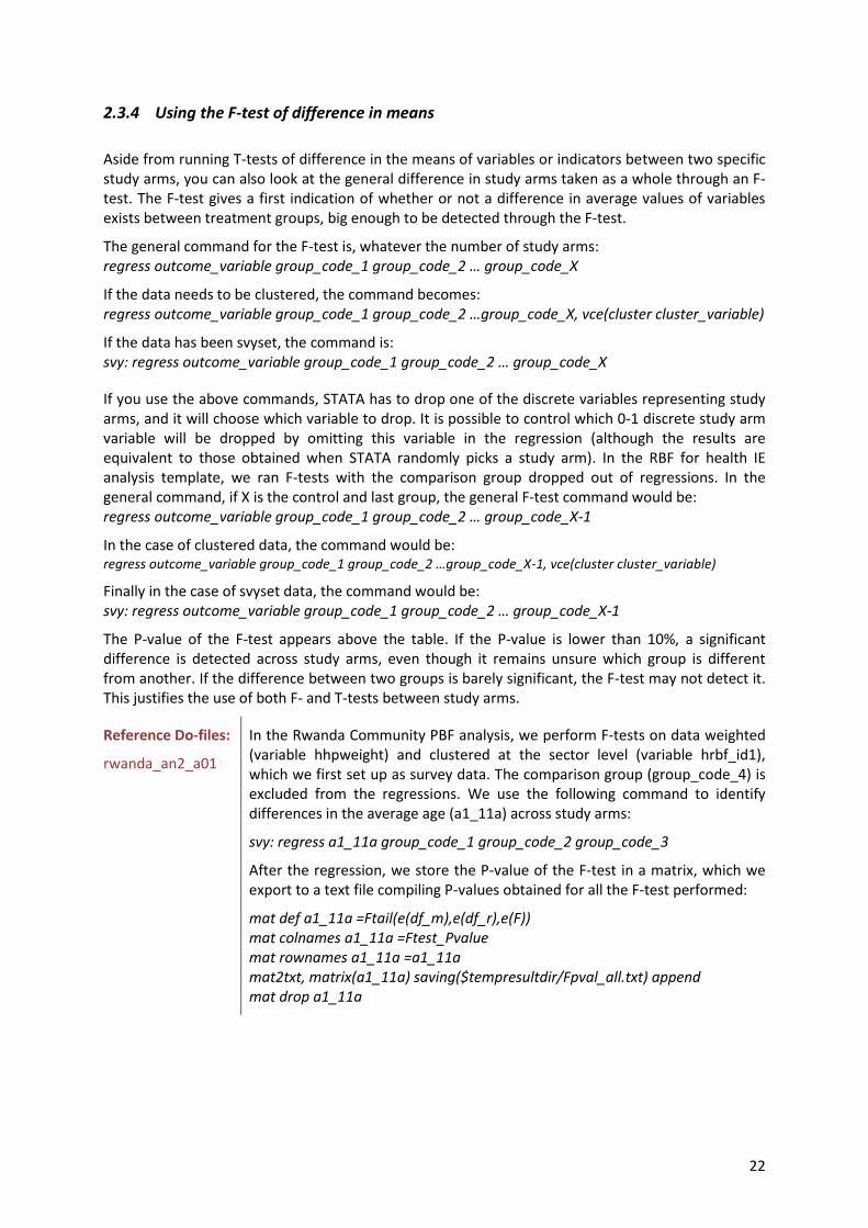
2.3.4 Using the F-test of difference in means

Aside from running T-tests of difference in the means of variables or indicators between two specific study arms, you can also look at the general difference in study arms taken as a whole through an F-test. The F-test gives a first indication of whether or not a difference in average values of variables exists between treatment groups, big enough to be detected through the F-test.

The general command for the F-test is, whatever the number of study arms: regress outcome_variable group_code_1 group_code_2 … group_code_X

If the data needs to be clustered, the command becomes: regress outcome_variable group_code_1 group_code_2 …group_code_X, vce(cluster cluster_variable)

If the data has been svyset, the command is: svy: regress outcome_variable group_code_1 group_code_2 … group_code_X

If you use the above commands, STATA has to drop one of the discrete variables representing study arms, and it will choose which variable to drop. It is possible to control which 0-1 discrete study arm variable will be dropped by omitting this variable in the regression (although the results are equivalent to those obtained when STATA randomly picks a study arm). In the RBF for health IE analysis template, we ran F-tests with the comparison group dropped out of regressions. In the general command, if X is the control and last group, the general F-test command would be: regress outcome_variable group_code_1 group_code_2 … group_code_X-1

In the case of clustered data, the command would be: regress outcome_variable group_code_1 group_code_2 …group_code_X-1, vce(cluster cluster_variable)

Finally in the case of svyset data, the command would be: svy: regress outcome_variable group_code_1 group_code_2 … group_code_X-1

The P-value of the F-test appears above the table. If the P-value is lower than 10%, a significant difference is detected across study arms, even though it remains unsure which group is different from another. If the difference between two groups is barely significant, the F-test may not detect it. This justifies the use of both F- and T-tests between study arms.

Reference Do-files:

rwanda_an2_a01

In the Rwanda Community PBF analysis, we perform F-tests on data weighted (variable hhpweight) and clustered at the sector level (variable hrbf_id1), which we first set up as survey data. The comparison group (group_code_4) is excluded from the regressions. We use the following command to identify differences in the average age (a1_11a) across study arms:

svy: regress a1_11a group_code_1 group_code_2 group_code_3

After the regression, we store the P-value of the F-test in a matrix, which we export to a text file compiling P-values obtained for all the F-test performed:

mat def a1_11a =Ftail(e(df_m),e(df_r),e(F)) mat colnames a1_11a =Ftest_Pvalue mat rownames a1_11a =a1_11a mat2txt, matrix(a1_11a) saving($tempresultdir/Fpval_all.txt) append mat drop a1_11a

23

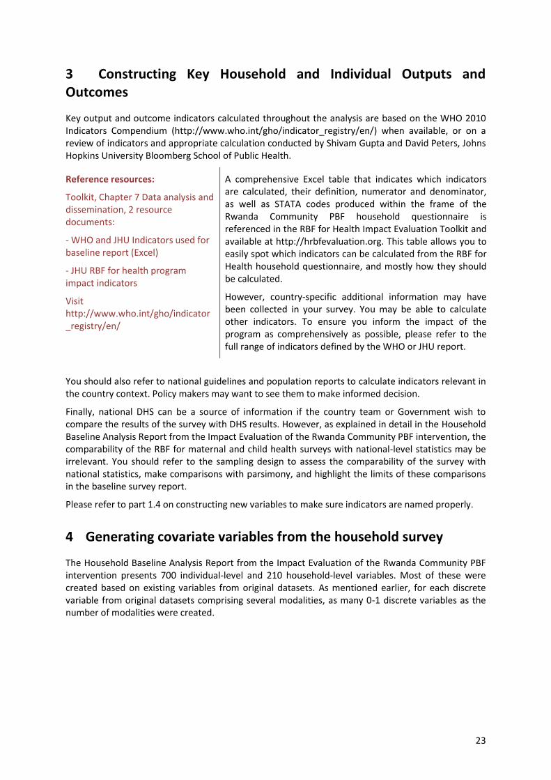
3 Constructing Key Household and Individual Outputs and Outcomes

Key output and outcome indicators calculated throughout the analysis are based on the WHO 2010 Indicators Compendium (http://www.who.int/gho/indicator_registry/en/) when available, or on a review of indicators and appropriate calculation conducted by Shivam Gupta and David Peters, Johns Hopkins University Bloomberg School of Public Health.


Toolkit, Chapter 7 Data analysis and dissemination, 2 resource documents:

- WHO and JHU Indicators used for baseline report (Excel)

- JHU RBF for health program impact indicators

Visit http://www.who.int/gho/indicator_registry/en/

A comprehensive Excel table that indicates which indicators are calculated, their definition, numerator and denominator, as well as STATA codes produced within the frame of the Rwanda Community PBF household questionnaire is referenced in the RBF for Health Impact Evaluation Toolkit and available at http://hrbfevaluation.org. This table allows you to easily spot which indicators can be calculated from the RBF for Health household questionnaire, and mostly how they should be calculated.

However, country-specific additional information may have been collected in your survey. You may be able to calculate other indicators. To ensure you inform the impact of the program as comprehensively as possible, please refer to the full range of indicators defined by the WHO or JHU report.

You should also refer to national guidelines and population reports to calculate indicators relevant in the country context. Policy makers may want to see them to make informed decision.

Finally, national DHS can be a source of information if the country team or Government wish to compare the results of the survey with DHS results. However, as explained in detail in the Household Baseline Analysis Report from the Impact Evaluation of the Rwanda Community PBF intervention, the comparability of the RBF for maternal and child health surveys with national-level statistics may be irrelevant. You should refer to the sampling design to assess the comparability of the survey with national statistics, make comparisons with parsimony, and highlight the limits of these comparisons in the baseline survey report.

Please refer to part 1.4 on constructing new variables to make sure indicators are named properly.

4 Generating covariate variables from the household survey

The Household Baseline Analysis Report from the Impact Evaluation of the Rwanda Community PBF intervention presents 700 individual-level and 210 household-level variables. Most of these were created based on existing variables from original datasets. As mentioned earlier, for each discrete variable from original datasets comprising several modalities, as many 0-1 discrete variables as the number of modalities were created.

24

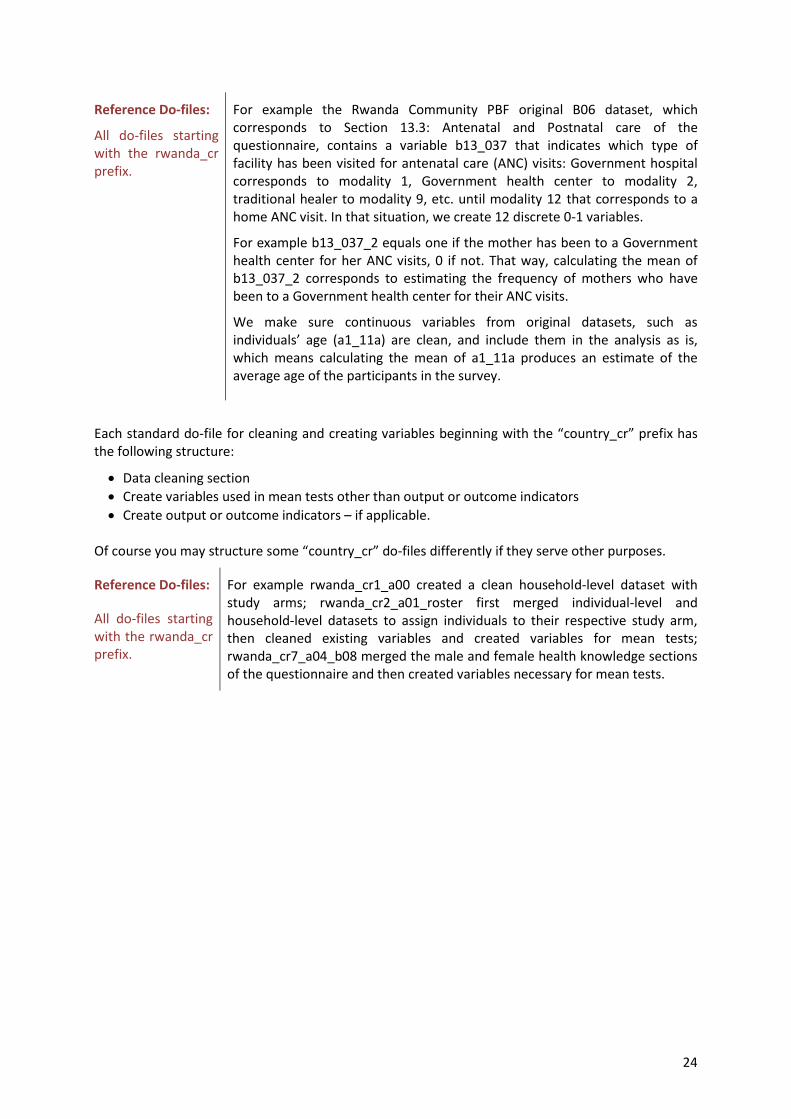
Reference Do-files:

All do-files starting with the rwanda_cr prefix.

For example the Rwanda Community PBF original B06 dataset, which corresponds to Section 13.3: Antenatal and Postnatal care of the questionnaire, contains a variable b13_037 that indicates which type of facility has been visited for antenatal care (ANC) visits: Government hospital corresponds to modality 1, Government health center to modality 2, traditional healer to modality 9, etc. until modality 12 that corresponds to a home ANC visit. In that situation, we create 12 discrete 0-1 variables.

For example b13_037_2 equals one if the mother has been to a Government health center for her ANC visits, 0 if not. That way, calculating the mean of b13_037_2 corresponds to estimating the frequency of mothers who have been to a Government health center for their ANC visits.

We make sure continuous variables from original datasets, such as individuals’ age (a1_11a) are clean, and include them in the analysis as is, which means calculating the mean of a1_11a produces an estimate of the average age of the participants in the survey.

Each standard do-file for cleaning and creating variables beginning with the “country_cr” prefix has the following structure:

Data cleaning section

Create variables used in mean tests other than output or outcome indicators

Create output or outcome indicators – if applicable. Of course you may structure some “country_cr” do-files differently if they serve other purposes.

Reference Do-files:

All do-files starting with the rwanda_cr prefix.

For example rwanda_cr1_a00 created a clean household-level dataset with study arms; rwanda_cr2_a01_roster first merged individual-level and household-level datasets to assign individuals to their respective study arm, then cleaned existing variables and created variables for mean tests; rwanda_cr7_a04_b08 merged the male and female health knowledge sections of the questionnaire and then created variables necessary for mean tests.

world bank human development network health, nutrition and...

Documents