Policy Ress ich 1WORKING PAPfRS.

Intrnatlona! Economic Analysisand Prospects

International Economics DepartmentThe World BankSeptember 1993

WPS 1187

How Should Sovereign DebtorsRestructure Their Debts?

Fixed Interest Rates, FlexibleInterest Rates, or Inflation-indexed

Andrew Warner

The presumption that fixed-rate debt is, in general, less riskythan flexible-rate debt is historically inaccurate. In some com-mon circumstances, flexible-rate borrowing actually reducesnet risk - whether debt service payments are indexed tonominal interest rates or to inflation in industrial countries.

Policy RauerWodkinsPopcddieuminatedsc fidingayof doik wp10gm.e.X s &xdn sam 7biadulleb i.d in dswynt Thmpapma, diai! bdy dwR.aaziAdiory Staff. caiy diesna of habcu.rui3a

andabul_d be md adcitdcodnl,h.fdinp. ,aiv n coum m-a3oou Thq'Aaab. audmed to the ieldd uik. BaDad dDioa, is uuu. _$_ey alias uan,bmw; aI

,a, .. .- . . .

Pub

lic D

iscl

osur

e A

utho

rized

Pub

lic D

iscl

osur

e A

utho

rized

Pub

lic D

iscl

osur

e A

utho

rized

Pub

lic D

iscl

osur

e A

utho

rized

Pokby Rswbol

InrSoa Eoonombc Anlysand Prospect

WPS 1187

This paper - a product of the Intemational Economic Analysis and Prospects Division, InternationalEconorncs Department - is part of a larger effort in the department to understand the links between theinternational economic environment and the growth process in developing countries. Copies of the paperare available free from the World Bank, 1818 H Street NW, Washington, DC 20433. Please contactJacquelyn Queen, room S8-216, extension 33740 (September 1993, 35 pages).

Can developing countries affect the variance of The worst-case scenario for developingreal imports solely by altering the way debt countries is flexible interest rate borowingservice is paid? The answer, says Warner, is a combined with monetary contraction in thequalified yes. industrial world, which raises nominal interest

rates, reduces inflation, and wors,ns the terms of-Te presumption thiat fixed-rate debt is less trade of developing countries. To the extent that

risky than flexible-rate debt is historically developing countries want to avoid this scenario,inaccurate as a general proposition. Using annual borrowing at either fixed interest rates or infla-data for 1970-90, Warner shows that for many tion-indexed rates would be preferable to bor-developing countries, flexible-rate borrowing rowing at flexible nominal interest rates.actually reduced net risk - whether debt servicepayments were indexed to nominal interest rates To reduce risk, countries should seek debtor to inflation in industrial countries. The contracts in which debt service payments varycovaiiance terms are larger and more often positively with their terns of trade. Resultspositive with inflation than with nominal interest indicate that inflation-indexed debt is mostrates. desirable on this score.

Wamer presents a macro-model of the Warner examines only extreme options, withindustrial countries to organize thoughts about all debt of one type. The optimal strategy wouldthe comovements of these variables in response probably entail all three kinds of borrowing.to shocks. The termns of trade of developing And the paper does not examine options forcountries are linked to this model by the assump- efficient intemational ri-k-sharing.tion that the level of demand in industrialcountries positively affects the terms of trade ofdeveloping countries.

ThnPrSedhe Policy Research DaperSeiesdissernianaes diefindings of wo Ckunder wayin therBanL Anobjoctveof the saiesis to Set these findings out quiclcly, even if presentations are less dhv fully polished. The findings, intMetatiom nsudconclusions in these papers do not necessaily represent of ficial Bank policy.

Produced by the Policy Researh Dissemiuition Center

.How Should Sovereign Deb.ors Restructure their Debts:Fixed Interest Rates. Flexible Interest Rates. or Inflation-Indexed?

Andrew Warner

Room S-8018International Economics Department

The World BankWashington, DC 20433

1. Introduction,

Should risk averse sovereign debtors borrow at fixed or flexible rates? And if borrowing at

flexible rates, rather than paying a fixed premium over a nominal interest rate like LIBOR, would it be

in the interests of the country to pay instead a fixe-d premium over the inflation rate in the currency of

the lending bank?

These questions have gained renewed importance as several debtors have already shifted, or are

now actively considering a shift from flexible to fixed rate debt. This shift is motivated by the belief that

fixed rate borro"'ing is less risky than flexible rate borrowing, and that in particular, it helps insure

debtors against a repeat of 1982, when the combination of flexible rate borrowing, high nominal interest

rates, and declining terms of trade helped precipitate the debt crisis. At issue is whether this presumption

is warranted after framing the question in a more general framework that does not exclusively rely on

the 1982 example.

Consider briefly the choice between fixed interest rate debt and flexible interest rate debt. To

decide the issue for a given country, it would be helpful, although perhaps infeasible, to know both the

future path of nominal interest rates and the covariance between interest rates and other sources of

income. For concreteness, assume that the country desires both low debt service payments and a low

variance of its real purchasing power over imports. The future path of interest rates matters because one

may wish to lock in now if rates are temporarily low, and borrow at flexible rates if they are temporarily

high. The covariance matters because if it is -2sitve and sufficiently large, then floating rate debt can

actually reduce the overall variance of real imports, and in this sense be less risky than fixed rate debt.

The purpose of this paper is to flag some of the relevant macroeconomic issues and to provide

useful gu.delines for policy makers dealing with these issues.

Since all recommendations require clarity about the objectives, this paper begins by assuming that

the objective is to minimize the variance of real purchasing power over imports, although some other

I

objectives are also considered. It is worth stating explicitly that this objective is best suited to the case

where countries have inherited debt, and have little ability to borrow and lend on international capital

markets to insulate real imports against the effects of temporary shocks. Clearly if countries could

borrow freely, then borrowing would be a simnpler way to deal with temporary interest rate shocks and,

consequently, the choice of debt contract would De less importan.. The assumption is also best suited to

the case where countries import essential intermediate inputs ind capital goods. In this situation, a shock

to interest payments can also become a supply shock by compressing essential imports, which would have

further ramifications on the real side or the economy. However, both of these cases, limited access to

global credit markets, and a high intermediate and capital goods content of imports, are arguably

important facts that currently confront developing countries.

To place this paper in a wider context, it is part of a literature that looks at ways developing

countries can reduce their exposure to risk from fluctuating export prices. There are three broad

approaches to this problem. The first is to seek ways to intervene in the market to control export prices.

Examples include buffer stocks and funds, quotas and variable expo. taxes. There is already an

extensive literature analyzing and criticizing these schemes (see Newbery and Stiglitz, 1981). A second

approach is to make better and more extensive use of market mechanisms for managing risks, such as

insurance markets, forward, futures and options markets. But several authors, (see Arrow, 1974), argue

that there are entrenched sources of market failure that make replication not possible with Ulese

instruments for developing countries. A third alternative is to design financial instruments that can serve

as hedging instruments in addition to their function as financing instruments. Examples include swaps,

commodity-linked bonds and indexed variable rate loans. With the possible exception of the recent past,

developing countries have not made full use of the range of feasible instruments.

Within this last alternative, the merits and demerits of commodity-linked bonds have been

examined by Meyers (1990). This scheme is best suited for countries whose exports are dominated by

2

homogenous commodities. In the case where countries expurt a range of commodities and where the

composition changes over time, it is less obvious how to implement such a scheme.

To avoid analyzing what the literature has already covered, this paper does not consider

commodity-linked bonds, and instead focusses on three options which are closer to what developing

courtriec are already Hoing or at least closer in spirit. The three options are, first, borrowing at fixed

interest rates without any indexing; second, indexing to a nominal interest rate; and finally, indexing to

an inflation rate. The last option is not commonly considered, but the paper will show a case where it

can achieve better diversification than nominal interest rate indexing. Essentially it amounts to

guaranteeing a fixed real interest rate to the creditor bank, since the interest rate paid can be set at a fixed

markup over inflation in the home curreacy of the bank.

1. The Countries.

To provide an idea of the list of countries that such a question woul *e relevant for, table I

presents statistics on the amount of commercial bank debt and variable rate debt. The country list is

restricted to countries that owed at least 5 percent of their long term debt to commercial banks in 1991.

The debt data are expressed in millions of US dollars.

3

Table 1. The ;mportance of Commercial Bank Debt and Variable Rate Debt, 1991

Long Term Percent to Percent atCOUNTRY Debt (LDOD) Commercial Banks Variable Rates

AGO.ANGOLA 7370 10.3 6.5ARG.ARGENTI 47188 49.0 58.3BGR.BULGARI 11023 47.6 73.0BOL.BOLIVIA 3676 9.8 24.2BRA.BRAZIL 95130 54.3 71.8BRB.BARBADO 483 37.3 24.6CHL.CHILE 14744 60.4 76.6CHN.CHINA 50502 29.4 33.1CIV.COTE DI 15167 48.9 65.7CMR.CAMEROO 5254 11.0 18.7COG.CONGO 3989 10.5 27.3COL.COLOMBI 15617 33.7 50.6CRI.COSTA R 3620 8.9 32.1CSK.CZECHOS 5846 43.0 33.3CYP.CNPRUS 1513 28.0 31.0DOM.DOMINIC 3554 24.2 31.5DZA.ALGERIA 26557 20.0 41.6ECU.ECUADOR 10094 50.0 61.0FJI.FIJI 346 24.3 31.5GAB.GABON 2935 6.2 10.2GTM.GUATEMA 2230 12.3 16.8GUY.GUYANA 1554 5.1 10.4HND.HONDURA 2940 7.8 21.7HTI.HAITI 609 7.6 0.7HUN. HUNGARY 19221 42.3 56.4IDN.INDONES 59960 27.9 43.1IND.INDIA 64315 13.3 21.0IRN.IRAN, 1 2736 38.6 84.7JAM.JAMAICA 3779 8.3 25.7JOR.JORDAN 7570 15.9 28.2KEN.KENYA 5776 27.1 20.2KOR.KOREA, 29318 36.8 41.8LBR.LIBERIA 1127 15.5 10.9LKA.SRI LAN 5758 6.9 5.6MAR.MOROCCO 20332 16.6 52.5MEX.MEXICO 83891 15.3 45.9MUS.MAURITI 960 28.9 11.0MYS.MALAYSI 18753 34.3 52.2NER.NICER 1503 16.1 16.4NGA.NIGERIA 33588 17.7 31.8NIC.NICARAG 8703 14.9 25.9OMN.OMAN 2270 71.3 59.6PAN.PANAMA 3939 54.1 61.3PER.PERU 15298 25.8 27.8PHL.PHILIPP 25893 28.1 4,.7PNG.PAPUA N 2565 46.6 52.7POL.POLAND 44057 23.1 67.7PRT.PORTUGA 20170 46.0 27.0PRY.PARAGUA 1800 16.6 16.8SDN.SUDAN 9717 21.4 19.6SLV.EL SALV 2069 8.0 14.1SYC.SEYCHEL 154 16.2 8.4THA.THAILAN 23336 54.0 56.6TTO.TRINIDA 1817 32.0 51.7TUN.TUNISIA 7369 6.7 23.4TUR.TURKEY 41135 33.2 35.5URY.URUGUAY 3128 20.6 60.1VEN.VENEZUE 28839 13.1 62.7YUG.YUGOSLA 15872 56.5 75.1ZAR.ZAIRE 9151 5.7 11,.37ur 7TURaDU AR ,R

Debt i, measLred in millions of 1991 U.S. dollars. Sour^e: World Bank: World Debt Table., 1992.

2. When will flexible rate debt be less risky than fixed rate debt?411

It was mentioned in the introduction that flexible rate debt may actuaily be less risky than fixed

rate debt as long as the covariance term is large enough to overcome the higher variability of flexible rate

debt. Of course, this may hold for either of the two kinds of flexible rate debt, nominal interest rate

indexed or intlation indexed, but the equations below are written for the case of nominal interest rate

indexing. This section derives a condition on the covariance term to gauge when flexible rate borrowing

has a lower variance that fixed rate borrowing, and then examines data to determine the extent to which

this criterion was satisfied in the past.

First, let P i md Pm represent aggregate export and import price indexes with 1987=1.0; let x

represent real expor:s in billions of 1987 dollars; let i and 8 represent the nominal interest rate on

outstanding debt and the fraction of principal that is repaid each year; and let D renresent outstanding

debt in billions of 19P7 dollars. Then the quantity of real imports that can be purchased in a given year

without borrowing is simply:

P.X D-x- (i+6)-pP. P.,

To simplify the notation and the analysis slightly, assume 0=0 and rewrite the expression as

follows.

z = px - id

Where p is the terms of trade, x is real imports, and d is real debt measured in terms of the

aggregate import good. Taking exports and debt as pre-determined, and the terms of trade and the

nominal interest rate as stochastic, the variance of real import purchases under flexible rate borrowing

would be:

5

Var(px - d) = x2Vart.p) + d2 Var(i) - 2xdCov(p,i)

And the variance under tixed interest rate borrowing would be:

Var(px - id) = x2Var(p)

Hence flexible rate borrowing can achieve a lower variance of real impoa purchases wvhen

d2 Var(Q) - 2xdCov(p,i) < 0.

Re-writing this condition, we have

Cov(p,a) > d (6)Var(i) 2x

To interpret this condition, note first that the coefficient from a simple bivariate regression of the terms

of .rade on nominal interest rates provides an estimate of the left hand side; and the right hand side is

simply one-half the debt to export ratio. Hence the condition states that flexible rate borrowing will be

less risky than fixed interest rate borrowing if the regression coefficient is positive and exceeds one half

the debt export ratio.

The next question is whether this condition has been satisfied in practice. To answer this

question, table 2 reports sample estimates of the left hand side of (6), denoted by #, using both a

representative nominal interest rate (Dollar LIBOR ' ate) and inflation (US inflation using the GDP

deflator). The estimates of the ,E's use 20 years of annual data covering the period 1970-1990; and the

estimates of the term d/2x uses 1990 data. The debt term (d) is total long term debt owed to commercial

banks in 1990.

6

The evidence indicates that when the O's are estimated using neminal interest rates, the irequality

is satisfied in about a third of the cases (21 out of 61 countries); using infl tion the inequality is satisfied

in just under 90 percent of the cases (54 of 61). Therefore, the past twenty years of data indicate that

in many countries inflation-indexed debt is more likely to satisfEy the lower variance criteria than interest-

rate-inJexed debt. Also notice that the estimates of 0 are typically sufficiently large that the question of

whether (6) is satisfied does not hinge important!y on the debt rm used to compute d/2x.

7

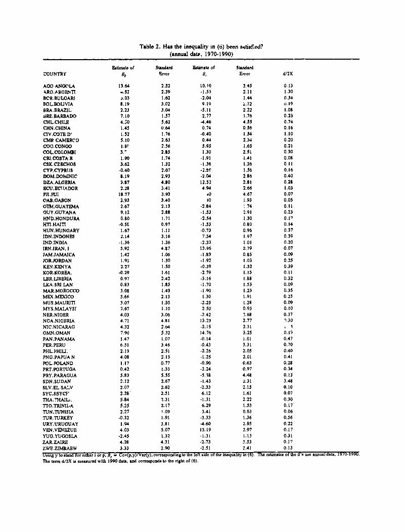
Table 2. Has the inequality in (6) been stfisfied?(annual dat., 1970-1990)

EBtiumte of Standard Estimut, of StandardCOUNTRY ,IS Error ,6 Ernor d/2X

AGO ANGOLA 13.64 2.52 10,10 2.45 0.13ARM.AROENTI -.52 2.39 -1.33 2.11 1.30BCR.BULOARI . 03 1.62 -2.04 1.44 0.34BOL.BOLIVIA S.19 3.02 9.19 2.32 U.19BRA.BRAZII. 2.23 3.04 -5.12 2.22 1.08JRE,BARBADO 7.10 1.57 2.77 1.76 0,23CHL.CHILE 4.;0 5.62 -4.46 4.55 0.74CHN.CHINA 1,45 0.64 0.74 0.56 0.16CIV.COTE D' 1.52 1.76 -0.40 1.54 1.10CMR CAMERCO 5.10 2.63 0.44 2.34 0.20COO.CONOO I.Sf, 2.56 5.95 1.65 0.21COLCOLOMDI 3.' 2.85 1.30 2.51 0.30CRI.COSTA R 1.90 1.74 -1.91 1.41 0.08CSK,CZBCHOS 3.62 1,32 -1.36 1.26 0.1lCYP.CYPRtIS -0.40 2.07 -2.S9 1.56 0.16DOM.DOMINIC 8.19 2.93 -2.04 2.86 0.40DZA.ALOERIA 3.87 4.80 12,52 2.81 0.28ECU.ECtIADOR 2.28 3.41 4.94 2.66 1.03Ffl.IJi .1877 3.93 40 4.67 0.07OAB.GABON 2.93 3.40 10 1.93 0.05OTM.GUATEMA 2.67 2.13 -2.84 1.74 0.11GUY.GUYANA 9.12 2.88 -1.53 2.91 0.23HND.HONDURA 0.80 1.71 -2.54 1.30 0.17HTI.HAI -0.5St 0.97 -1.53 0.80 0.14HUN.HUNGARY 1.67 1.11 -0.73 0.96 0.37IDNINDONES 2.14 3.16 7.54 1.97 0.39INDINDIA -1.36 1.36 -2.33 1.01 0.20IRN.IRAN, 1 5.92 4.87 13.96 2.79 0.07JAM.JAMAICA 1.42 1.06 -1.83 0.85 0.09JOR.JORDAN 1.91 1.30 -1.92 1.03 0.25KEN.KENYA 2.27 1.50 .0.39 1.32 0.39KOR.K.OREA, -0.29 1.61 -2.79 1.15 0.11LBR.LIBERIA 0.97 2.42 -3.16 1.88 0.32LKA.SRI LAN 0.83 2.85 -1.70 1.53 0.09MARMOROCCO 3.08 1.43 -1.90 1.23 0.35ME.MEXICO 3.66 2.13 1.30 1.91 0.23MUS.MAURITI 3.07 1.50 -2.25 1.28 0.09MYS.MALAYSI 2.67 1.10 2.50 0.93 0.10NER.NIGER 4.03 3.06 -2.42 7.68 0.37NGA.NIGERIA 4.71 4.81 13.23 2.77 ".30NIC.NICARAG 4.32 2.64 -2.25 2.31 . IOMN.OMAN 7.90 5.32 14.76 3.25 0.19PAN.PANAMA 1.47 1.07 -0.14 1.01 0.47PER.PERU 6.51 3.46 -0.43 3.31 0.70PHL.PHI- ' 2.13 2.51 -2.26 2.05 0.40PNG.PAPUAN 4.08 2.13 -1.25 2.01 0.41POL.POLAND 1.17 0.77 -0.90 0.63 0.28PRT.PORTUGA 0.42 1.33 -2.24 0.97 0.34PRY.PARAGUA 5.83 5.55 -5.38 4.48 0.13SDN.SUDAN 2.12 2.67 -1.43 2.31 3.48SLV.EL SA-V 2.07 2.62 -2.33 2.15 0.10SYC.SEYC} 2.28 2.51 6.12 1.61 0.07THA.THAIL'. 5.84 2.31 -1.31 2.22 0.307T0.TRINIbA 5.25 2.17 6.29 1.53 0.17TUN.TUNISIA 2.27 1.09 3.41 0.63 0.06TUR.TURKEY -0.32 1.91 *3.33 1.36 0.56URY.URUGUAY 1.94 3.81 -4.60 2.95 0.22VEN,VENEZUE 4.03 5.07 13.19 2.97 0.17YUU.YUJOSLA -2.45 1.32 -1.31 1.13 0.31ZAR.ZAIRE 4.28 4.31 -2.73 3.53 0.17ZWE.ZIMBABW 3.33 2.90 -2.51 2.41 0.13Using y to stand for either a orp, p, - Cov(p,y)/Vaf(y), correapoiagto the left side of the inequality in (6). The estimates of the W's use annual data, 1970-1.The term d/2X is measured with 1990 data, and corresponds to the right of (6).

The data summarized in the precediag section show that the covariance terms have been large

enough to make a difference. Given this evidence, this section presents a model to tiirnk more

systematically about the ultimate sources of co-r.ovements between the key economic variables. The

model is a closed economy model of the OECD block which determines OECD nominai interest rates and

inflation as a function of exogenous monetary policy, fiscal policy and oil price variables. Developing

economies ar- linked to this block with the assumption that their terms of trade respond to the level of

demar.d in the developed world.

The model may be seen as a leaner version of more elaborate models suAh as McKibbin and

Sachs, 1991. Since the main purpose is expository, I have dclberately ehosen simp;ifications which focus

on the main points. All of the qualitative effects which underlie the conclusions io this paper have been

replicated with simulations of the McKibhib and Sachs model.

To repeat, the model determines the three main variables of interest, nominal interest rates,

OECD inflation, and the external terms of trade of less developed countries, and distinguishes between

short run and long run effects. IThe exogenous variables are an OECD fiscal variable, g, a money supply

variable, m, and world oil prices, pO. All variabies are in natural logs.

9

y = f3y - a(i - p) + g (7)

m -p e Oy - xi (8)

P=Y(Y - (9)

P, = y (10)

= -,po.l (11)

Equation (7) is a semi-reduced form equilibrium condition for the goods market. Aggregate

demand on the right hand side is a function of output, the real interest rate, and a fiscal variable.

Equation (8) is a conventional money market equation, where money demand depends on output and the

opportunity cost of holding money, given by the nominal interest rate. Equation (9) is a simple Phillips

curve that expresses inflation as a function of the gap between current output and potential outptut. The

assumption is that the OECD price level, p, cannot jump in response to shocks in the short run, and

instead adjusts gradually over time according to (9). In this sense the model shares the price stickiness

assumption uf static Keynesian models. Equation (10) (with p, representing the terms of trade of

developing countries) embodies a purely demand side view of terms of trade determination. And equation

(I1) is a production function where labor and capital are not written explicitly, since they will be held

constant in the experiments. The price of oil is modelled to reduce potential output because it is a key

10

intermeJaae in OECD economies. This is similai to the way oil prices are treated in Bruno and Sachs

(1985), and is supported by econometric evidence that energy and capital are complements, (see Berndt

and Wood (1979)).

Although the main points of the model will be presented graphically, it is worth documenting the

algebraic solution in addition. Treating the long run or steady state solution first, inflation is zero by

assumption and hence output equals potential output from equation (9). Equations (7) and (8) then jointly

determine the long run level of nominal interest rates and the price level. The full solution is in equations

(12) to (17) below.

p =0 (12)

y = Poil (13)

Y = (14)

i = 1 (g - (1-p)T) (15)

p = _g _r[ (1) + } + m (16)

P,=Y (17)

Of this set of equations, the most relevant for the question at hand is the nominal interest rate

11

equation (15). It is worth noting that since inflation is zero, this equation is also a real interest rate

equation. Note that real interest rates are permanently raised by a permanent rise in government

spending. The reason is that with output fixed at its full employment level, the real interest rate must

rise to shift demand from the private sector to the government. A rise in oil prices also raises the real

interest rate in the long run because it reduces value-added output, and with nothing else changing on the

demand side, real interest rates must rise to bring demand to this lower level (the term l-$ is assumed

to be a positive fraction). Finally, a rise in the money supply increases p proportionally in the long run

and has no effect on the other variables of interest.

According to this model one would not want to borrow at flexible interest rates if a fiscal

expansion is anticipated, since this will simply raise OECD interest rates and developing country debt

service payments. It is also clear that an oil price increase is the worst of all possible outcomes for non-

oil exporting developing countries, since both OECD output and developing country commodity prices

will fall at the same time that OECD interest rates rise. If such an event is anticipated, then fixed rate

borrowing will at least insulate developing countries from higher future interest rates. On the other hand,

flexible rate borrowing would be better if oil prices were expected to come down, since the future interest

rate decline would work in favor of indebted developing countries.

Between steady state's, the price level is treated as a slowly adjusting variable whose motion is

governed by equation (9). Hence (7) (8) and (9) are solved simultaneously for output, nominal interest

rates and inflation. The solution is given below.

P = r(Y - i) (18)

-pp,i (19)

12

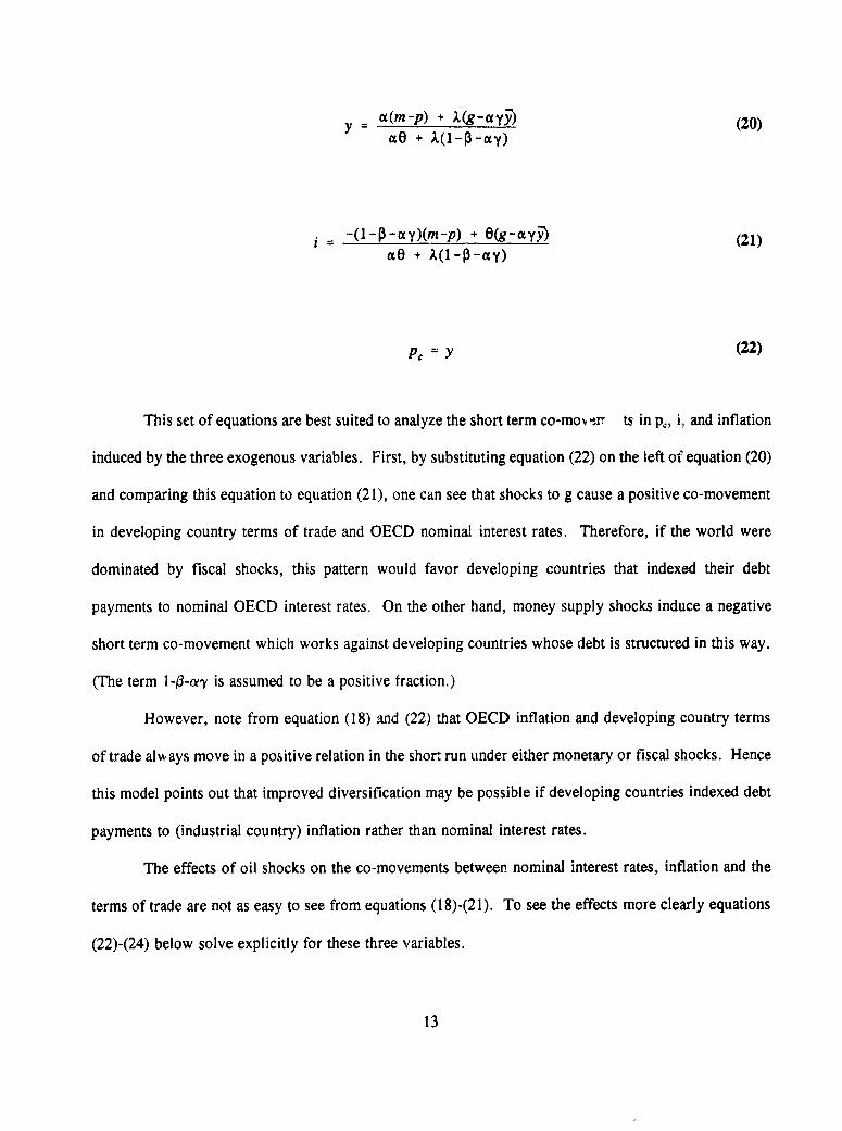
y c (m-p) X(g-cey5) (20)ote + A(l ay)

-(O--eay)(m-p) + 0(g-ayD) (21)ae + A(1-P-ay)

P, = Y (22)

This set of equations are best suited to analyze the short term co-movelr ts in pc, i., and inflation

induced by the three exogenous variables. First, by substituting equation (22) on the left of equation (20)

and comparing this equation to equation (21), one can see that shocks to g cause a positive co-movement

in developing country terms of trade and OECD nominal interest rates. Therefore, if the world were

dominated by fiscal shocks, this pattern would favor developing countries that indexed their debt

payments to nominal OECD interest rates. On the other hand, money supply shocks induce a negative

short term co-movement which works against developing countries whose debt is structured in this way.

(The term l-0-cYy is assumed to be a positive fraction.)

However, note from equation (18) and (22) that OECD inflation and developing country terms

of trade always move in a positive relation in the shor. run under either monetary or fiscal shocks. Hence

this model points out that improved diversification may be possible if developing countries indexed debt

payments to (industrial country) inflation rather than nominal interest rates.

The effects of oil shocks on the co-movements between nominal interest rates, inflation and the

terms of trade are not as easy to see from equations (18)-(21). To see the effects more clearly equations

(22)-(24) below solve explicitly for these three variables.

13

(a(m-p + 1(g+ay AP,p,) + p (23)

e aO + l(1-0-UY)

-(1-p-cty)(m-p) + e(g+aypPop,) (25)

ae + X(l-P-ay)

It is clear from these equations that oil shocks will move all three variables in the same direction. Hence

the short run dynamics provide no basis on which to choose between inflation indexing and nominal

interest rate indexing, but both achieve a positive co-movement that fixed rate debt would not achieve.

Having outlined the analytical solution of the model in both the long and the short run, the

behavior of the model is summarized in figures I to 3, with figure I showing the response to a permanent

OECD monetary expansion, figure 2 showing the response a permanent OECD fiscal expansion and

figure 3 showing the response to a permanent rise in the price cf oil.

14

3. Summary of policy recommendations from the model.

The policy prescriptions from such a model regarding fixed versus flexible rate borrowing can

now be summarized (see also the summary in table 3). It should be stressed that these recommendations

take into account only the direction in which the key variables move in response to shocks. When

recommendations hinge on favorable co-movements between variables, it is implicitly assumed that the

condition in equation (6) is satisfied.

Money Supply shocks.

If you know that a monetary expansion is on the horizon, then flexible nominal rate borrowing

is oest: you will benefit from the commodity price boom; and nominal rates will come down. Fixed rate

borrowing simply will deprive you of the benefit from falling nominal rates. Inflation indexing is even

worse because inflation will rise and you will incur higher debt service payments as inflation rises.

If you know that a monetary contraction is on the horizon, then inflation indexing is best: you

will suffer a commodity price decline no matter what you do; but at least with inflation-indexing your

debt service payments will come down as inflation comes down. In contrast, flexible nominal rate

contracts expose you to higher debt service payments as nominal rates rise. Fixed rate contracts would

not expose you to higher debt service payments, but would not be as good as inflation indexing.

If you do not know which way OECD monetary policy will turn, and just want insurance against

any outcome, then inflation-indexed borrowing is best: the reason is that OECD inflation and commodity

prices will vary positively in response to either a monetary expansion or contraction. Neither fixed nor

flexible rate borrowing will achieve this kind of insurance.

Fiscal shocks.

If you know that a fiscal expansion is on the horizon, then fixed nominal rate borrowing is best:

you will benefit from the commodity price boom; and lock in at currently low rates now before they go

up. Flexible rate borrowing exposes you to interest rate increases both in the short and long term.

15

Inflation indexing is not as bad as interest rate indexing because the inflation increase would not be

permanent (as the interest rate increase will be), but is still worse than fixed rate borrowing.

If you know that a fiscal contraction is on the horizon, then flexible nominal rate borrowing is

best: the interest rate decline will cushion the decline in commodity prices, and you will benefit further

in the long run as interest rates stay low (while commodity prices recover as OECD output returns to

capacity). Fixed rdte borrowing will lock you in to temporarily high interest rates and is therefore a bad

idea. Inflation indexing is basically similar to nrminal interest rate indexing in the short run, but is not

as good in the long run because inflation will not stay low permanently as will nominal interest rates.

If you do not know which way OECD fiscal policy will turn, and just want insurance against any

outcome, then inflation indexing is best: the reason is that OECD inflation and commodity prices will

have a positive covariance under any fiscal shock. Neither fixed or flexible rate borrowing will achieve

this kind of insurance.

Oil price shocks:

Non-oil exporting developing countries.

If you know that oil prices will rise, then fixed interest rate contracts are best. In the long run,

the terms of trade will decline and interest rates will rise, so that flexible interest rate borrowiiig is bad

idea. Inflation indexing is less bad than nominal interest rate indexing because the rise in inflation will

not be sustained, but is still inferior to fixed rate borrowing.

If you know that oil prices will fall, then it is best to contract at flexible interest rates. In the

long run, the terms of trade will rise and interest rates will fall. Since interest rates will fall permanently

while inflation will not, inflation indexing is inferior to nominal interest rate indexing.

When oil price movements are uncertain, both forms of indexing are risky because the costs can

be quite high if oil prices increase. Hence fixed interest rate contracts are safer.

Oil-exporting developing countries.

16

If you know that oil prices will rise then fixed interest rate contracts are best because you will

avoid paying higher nominal interest rates. If you know that oil prices will decline, then flexible interest

rate contracts are best so that you can benefit from lower interest rates. If future oil prices are uncertain,

then note that both oil prices and nominal interest rates vary positively in both the short and long runs:

hence flexible interest rate contracts can provide insurance against large shocks to real imports.

17

Table 3. Summary of policy recommendations from the model

Contingencv Preferred contract

Expansion flexible i

Money Contraction inflation indexed

Insurance inflation indexed

Expansion fixed i

Fiscal Contraction flexible i

Insurance inflation indexed

Oil-importing countries:

Rise fixed i

Oil Price Fall flexible i

Insurance fixed i

Oil-exporting countries:

( Rise fixed i

Oil Prkie Fall flexible i

Insurance flexible i

4. Possible modifications to the model.

One possible objection to the model so far is that equation (10) assumes that the tcrms of trade

of developing countries is solely a function of dtemand in industrialized countries. An alternative

approach would be to emohasize that less developed countries tend to export commodities and thus use

a more explicit mode; of commodity price formation. For example, under the competitive model of

commodity price formation with storage, commodity prices would be affected by real interest rates in

addition to other variables. The reason is that if the commodities are storable, there is an arbitrage

equation equating the required rate of return (real interest rate) with expected capital gain in commodity

prices. Under this model, for a given level of expected future commodity prices, a rise in the real

interest rate would depress current commodity prices (this argument goes back to Hotelling, 1932).

How would the conclusions change if this effect (higher real interest rates depressing the terms

of trade) were added to equation (10)? First, this change would reinforce the conclusions regarding

monetary shocks. The reason is that a monetary expansion strongly depresses real interest rates, raising

commodity prices at the same time that it raises aggregate demand. Hence the real interest rate effect

would reinforce the demand effect on the terms of trade. However, with fiscal shocks the conclusions

would be reinforced in the short run but offset in the long run. The reason they would be offset is that

a permanent fiscal expansion raises real interest rates in the long run, thus lowering commodity prices

below the level they would obtain in the absence of the real interest rate effect. Finally, the addition of

real interest rate effects on commodity prices would offset the demand effects of oil price shocks. Higher

oil prices depress real interest rates in the short run and raise them in the long run; exactly the opposite

of the demand effect.

A second possible objection is that the model only incorporates the effect of oil prices on potential

output, to the exclusion of demand effects. To the extent that higher oil prices raise inflation and nominal

interest rates under-adjust to inflation, the model can yield lower real interest rates in response to oil price

19

increases. Since output in the short run is demand determined, these lower real rates stimulate demand

and output. This result of higher oil prices stimulating OECD output in the short run seems sharply at

odds with the evidence of the 1970s. To resolve this issue, oil prices could be directly added to the right

hand side of equation (7), to depress aggregate demand through income or wealth effects. The effect of

oil prices on output would then depend on the magnitude of parameters. However, since none of the

main conclusions of this paper depend on the short run output effects of oil prices, this modification is

not pursued.

20

5. Wealth effects and access to financing.

Earlier parts of this paper analyzed issues that come into play when countries cannot borrow

freely on international capital markets to finance temporary shocks to their balance of payments.

Different issues are relevant in the intermediate case where countries have some access to financing but

their access is sensitive to perceptions about the solvency of the country by potential creditors.

When a country experiences a decline in export revenues, and the decline is severe enough that

the international financial comnimnity questions the solvency of the country, it is important that the form

of debt contract the country has adopted does not exacerbate the situation by lowering the likelihood that

the country can obtain financing. This section presents a simple framework to show how this car happen,

and then asks what the evidence of the past 20 years suggests about the importance of the form of debt

contract for this issue.

It is first necessary to write some model of how the international financial community evaluates

a country's creditworthiness. For this purpose, assume that potential creditors use the present value

model to evaluate creditworthiness. That is, they compute the present discounted value of exp3rts and

debt service payments on the (admittedly naive) assumption that variables such as interest rates and

exports will remain constant in the future at current levels. This provides one possible measure of a

country's capacity to repay additional debt, and it is assumed further that access to financing depends on

the difference between this computation of export wealth and debt liability. This procedure is crude, but

it does have the virtue of matching what many allege is standard practice in country risk analysis in major

banks.

Concerning the asset side of this calculation, let current nominal exports be given by x(t) and let

the current (and therefore expected future) growth in nominal exports be r,(t). Using the current nominal

interest rate as the discount rate, nominal export wealth, W1 is finite as long as the discount rate exceeds

export growth,

21

W (t) = x(t) > ° (26)

and infinite if export growth exceeds the discount rate, i(t) - 7r,(t) < 0.

On the other side of the balance sheet, the countries' liabilities are the present discounted value

of expected future debt service payments. These payments differ according to the form of debt contract.

Abstracing from several details about the debt contracts, with flexible rate borrowing debt service

payments would essentially be i(t) * D(t), while under fixed interest rate borrowing they would be i * D(t)

and under inflatiosi indexing they would be ir(t) * D(t). The main point to note is that the interest rate

term cancels out of the present discounted value calculation with flexible interest rate borrowing but does

not under the two alternatives:

Under flexibl rate: f c -')' iD ds = D(t), (27)

Under fixed rate: e ez"1 iD ds = D(t), (28)

i(t)D()(9

Under an indexed rate: f e('-') 7rD ds =(tD(t) (29)

Combining these liabilities with the export wealth calculation in (26), the perceived net worth of

22

the country under the three kinds of borrowing (flexible interest rate, fixed interest rate, and inflation

indexed) can be represented as follows.

Under flexible rate: W = x D (30)

Underfixed rate: W = x. _ - (31)

Under an indexed rate: W = x _ D (32)i-7Cr ~x

These calculations are for the case where the interest rate exceeds export growth, which is

precisely the case where solvency can be questioned. In the other case when export growth is high,

solvency is less likely to be a real issue. The important point to note from equations (30) - (32) is that

the difference between them is due to the terms i/i and 7r/i in (31) and (32). Hence knowing more about

the relationship between shocks to export wealth and shocks to these two terms is important in assessing

the contracts under question.

Annual data was collected on i (nominal LIBOR), 7r (US GNP deflator), x, and 7rt, for the 61

developing countries covering the years 1970-1990. Export wealth, Wx, was then calculated in all cases

where export growth was sufficiently low, 7rt < i. Since export growth was typically higher than i, this

condition reduced the number of usable observations sufficiently that it was decided to pool the data

rather than examine individual countries. We then look at the conditional distribution of A(i/i) and

4(7r/i) given that countries experienced negative shocks to export wealth (AWnV < 0).

The reason for conditioning on the event AWt<0 is that years in which export wealth declined

represent potential crisiL years in which financing may have been at risk. The debt contract woulk' soften

23

the blow in these years if liabilities as perceived by external financiers also declined during these years.

Therefore the more the conditional density is shifted to the left, the better.

Figures I and 2 present the empirical frequency distributions for the cases of inflation-indexed

and fixed interest rate borrowing (i is set at 0.05). On the basis of the evidence from the past 20 years

displayed in these figures, there are grounds for slightly preferring inflation indexing over the other kinds

of borrowing, but the evidence is not strong. The mean of the density in figure I is -0.000103, that of

figure 2 is 0.000815. Given the standard errors of 0.0011 and 0.0012 respectively, neither mean is

significantly different from 0 and the means are not significantly different from each other. Therefore,

although access to financing may be an important concern, there is not strong evidence from the past 20

years that the form of debt contract affects this significantly.

24

6. How much difference would inflation-indexing have made?

Much of this paper has suggested that inflation indexing would have been superior to nominal

interest rate indexir, or fixed interest rate borrowing. For example, the data in table 2 show that the

condition in (6), namely that Cov(p,j)/Var(j) > d/2x, is satisfied for a larger group of countries when

j = U.S. inflation than when j = U.S. nominal interest rates. In addition, when the world is dominated

by mon1etary shocks emanating from the high income economies, the model provides a reason to exect

that the terms of trade in low income economies will vary together with inflation in the high incoine

economies, but will vary inversely with nominal interest rates in the high income economies. Hence

under monetary shocks, the variance of equation (2), that is, the variance of z(j) = px - jd, should be

lower when j = inflation than when j = nominal interest rates, and in this sense inflation indexing should

achieve better insurance for lower income economies. The z's have welfare significance because they

measure the quantity of real imports that a country could purchase without any external borrowing or

lending.

Given these prior results, the next natural question is the following. Suppose developing

countries had their debt indexed to inflation rather than to nominal interest rates during the past 20 years.

How much difference would it have made? To answer this, z(j) = px - jd was simulated using actual

data for p, x, and d, combined with six alternatives for j. The first three of these were flexible interest

rate simulations, where j was the nominal 3-month government bond rate for Germany and Japan and the

3-month dollar LIBOR rate for the U.S.; and in the remaining three simulations, j was GDP-deflator

inflation for the same three countries plus a real interest rate markup. This markup was set equal to the

average ex-post real interest rate over the period 1970-1990, using the same interest rates and inflation

rates. Thiese real interest rates were 0.035 for Germany, 0.023 for Japan and 0.033 for the United States.

So for each developing country, six time series using annual data during the period 1970-1990 were

generated for z(), corresponding to j = (i0DrU,iJPN'USA' 7rDEU+O.O35,IrJPN+O.O23 ,rru,+ 0.033). Finally,

25

to eliminate the trend due to population growth, each time series of z(j) was divided by population in the

relevant developing country.

To compare the I-vo broad alternatives of borrowing at flexible nominal interest rates or inflation

indexing, table 4 reports sample variance ratios of the simulated z's divided by population. The first

column uses U.S. inflation and interest rates, the second uses German data and the third uses Japanese

data. Since in each column the numerator is the variance for inflation indexing, a value below 1.0 reveals

that inflation indexing would have entailed lower variance than interest rate indexing. The table shows

that there are many countries where this would have been, the case, and in some of these the difference

in variance would have been substantial. However, there is considerable dispersion across countries so

that generalizations are not very informative. But the table does show that the reduction in variance from

inflation-indexed borrowing can be substantial for particular countries.

26

Table 4. Inflation indexing versus interest rate indexing: variances

V(z(wvA+ 033))N(z(j,S)) V(z(wDg u+ 035)) N(r(6m)) V(z(,w .023))/N(z(i3)

ARG 0.61 0.94 0.89BOR 1.03 0.99 0.98BOL 0.79 0.97 0.86BRA 0.97 1.23 1.45CHL 0.89 1.02 1.18CHN 1.01 1.03 1.05CiV 0.82 0.86 0.76CMR 1.12 1.01 1.08COo 1.28 1.11 1.22COL 0.90 1.05 1.27CR] 0.60 0.83 0.75CSK 1.05 1.01 1.03DOM 0.79 0.92 0.77DZA 1.12 1.05 1.13ECU 1.01 1.04 1.10FJI 0.96 0.99 0.94GAB 0.96 1.00 0.98GTM 0.91 0.95 0.90GUY 0.88 0.91 0.82HND 0.85 0.87 0.80HTI 1.09 0.99 1.12HUN 1.12 1.12 1.19IDN 1.10 1.09 1.20IND 1.02 1.38 2.19IRN 1.00 1.00 1.00

JAM 0.69 0.75 0.70JOR 1.13 1.10 1.21KEN 0.83 0.87 0.75KOR 1.02 1.02 1.04LBR 0.93 0.94 0.89LKA 1.08 1.06 1.45MAR 0.69 0.87 0.71MEX 1.65 1.42 1.70MUS 1.00 1.01 1.02MYS 1.04 1.04 1.08NER 0.93 0.93 0.93NOA 0.98 0.99 0.98NIC 0.86 0.88 0.75PAN 1.09 1.07 1.14PER 0.96 0.94 1.01PHL 0.74 0.91 0.76PNG 0.92 1.02 0.80POL 1.01 1.18 1.27

PRT 0.99 1.03 1.06PRY 0.99 1.04 1.08SLV 0.89 0.94 0.90SYC 1.03 1.05 1.06THA 1.00 1.04 1.06rTO 0.98 0.97 0.95

TUN 1.16 1.16 1.26TUR 1.09 1.08 1.14URY 0.97 1.04 1.35VEN 0.99 1.01 0.99ZAR 0.94 0.93 0.84ZWE 0.93 0.94 0.88

Averge 0.97 1.01 1.04

7. Summary and main conclusions.

This paper basically attempts to answer the following question. Does theory and the evidence

from the past twenty years provide grounds for thinking that developing countries can affect the variance

of real imports soley by altering the way debt is paid? The answer is a qualified yes. More specifically,

the paper makes the following points.

The paper first shows that if there is a presumption that fixed rate debt is less risky than flexible

rate debt, then this presumption is historically inaccurate. For many developing countries, using annual

data over the period 1970-1990, the relevant covariance terms are sufficiently large that flexible rate

borrowing can actually reduce overall risk. This statement is true whether debt service payments are

indexed to industrial-country nominal intelest rates or inflation. But it is noteworthy that the covariance

terms are larger and more often positive with inflation than with nominal interest rates.

The paper then presents a macro-model of the industrialized countries to organize thinking about

the co-movements of these variables in response to shocks. The terms of trade of less developed

countries are linked to this model by the assumption that the level of demand in industrialized countries

positively affects their terms of trade. The model rules out causality running from the terms of trade of

developing countries to the indistrialized country equilibrium.

The worst case scenario for many developing countries is flexible interest rate borrowing

combined with a monetary contraction in the industrialized world. A monetary contraction raises nominal

interest rates, reduces inflation and reduces the terms of trade of developing countries. As happened in

the early 1980s, developing countries whose debt service payments depend on nominal interest rates will

suffer because the terms of trade decline at the same time that debt service payments rise. To the extent

that countries wish to avoid this scenario, either fixed interest rate debt or inflation indexing would be

preferable to borrowing at flexible nominal interest rates.

More generally, paper points out that to reduce risk countries should seek debt contracts where

28

debt payments vary positively with their terms of trade. Several of the results in this paper point to

inflation-indexed debt as being desirable on this score.

First, using eata from the period 1970-1990, the covariance between developing country terms

of trade data and OECD inflation is generally positive and larger than the covariance using nominal

interest rates. Second, the model offers a reason for this observation. Nominal interest rates in

industrialized countries should vary inversely with monetary shocks in industrialized countries, but

inflation in industrialized countries and the terms of trade of developing countries should -ary positively

with monetary shocks. To the extent that this kind of monetary shock was part of the mix of shocks

affecting the world economy in the past twenty years, the stronger positive relation between developing

country terms of trade data and OECD inflation than with OECD interest rates is not surprising. Third,

simulations using actual data indicate that many developing countries could have achieved less variation

in their imports if all of their debt was inflation-indexed rather than nominal interest rate indexed.

It is also worth pointing out what the paper does not do. First, the paper examines effects on the

variance of real imports rather than the mean or other aspects of the distribution. This is not to deny that

higher mean import purchases would be beneficial, instead it reflects scepticism that there is anythinig

constructive too add on this issue. Of course, if countries could lock-in their debt at a very low rate, then

they snould do so. But there is no strong reason to think that developing countries can out-forecast their

creditors about the future path of interest rates. Second, the paper examines only extreme options: either

the debt is all inflation indexed, all interest rate indexed or all fixed rate debt. The reason for doing so

is to bring out the contrasts between these options. It should be clear that the optimal strategy would

probably entail all three kinds of borrowing.

Finally, the paper does not analyze the issues from the perspective of the creditor banks, and

therefore does not fully examine risk sharing issues. For example, it may be the case that creditors

wouw- welcome the introduction of inflation-indexed bonds as an additional asset to minimize their own

29

risk, (these are not widely available in industrialized countries) and thus there may be some scope for

more efficient international risk sharing.

30

Figure 1. The time oath of nominal interest rates. inflation and commodity pricein response to a permanent monetary expansion in the OECD.

( P.

* I_

,. = _ _~~~~~tme

Figure 2. The time path of nominal interest rates. inflation and commodity pricesin response to a germanent fiscal exnansion in the OECD.

I ~ ~~ ;

PC~~~~~~~~~~~~~~~~~~~~~l

, -

Figure 3. Th- rim gath Qf nominl interet rates. inflation aad comodity prcjsin response to an oil rice inctease (or any adverse supply shozk) in the OECD,

r -7

1~~~~~~~~~~~~~~~

t

Figure 4. Conditional frequency distribution for inflation-indexed borrowing: f(4(w/i)fAW1 <O)

70equency

60 -

50 -

40

30

20

10

-3 -2 -1 0 1 2 3 4 5

* 1000

Figure 5. Conditional frequency distribution for fixed interest rate borrowing: f(A(0.05/i) AW3 < 0)

60

Frequency

50

40-

30-

20-

10

-4 -3 -2 -1 0 1 2 3

A(0.05/i) * 1000

References

Arrow, Kenneth J., (1974), "Limited Knowledge and Economic Analysis", American Economic Review64, 1-10.

Bruno, Michael, and Jeffrey D. Sachs (1985), Economics of Worldwide Stagflation, Harvard UniversityPress.

Hotelling, Harold, (1931), "The Economics of Exhaustible Resources", Journal of Political Economy,39, 137-175.

Meyers, Robert J. (1992) "Incomplete Markets and Commodity Linked Finance in Developing Countries"World Bank Research Observer, 7, January, 79-94.

Newbery, David M. G., and Joseph E. Stiglitz (1981), The Theory of Commodity Price Stabilizationi,Oxford, Oxford University Press.

Pindyck, Robert S. and Julio J. Rotemberg, (1990) "The Excess Co-movement of Commodity Prices",The Economic Journal, 100, December, 1173-1189.

Policy Research Working Paper Series

ContactTitle Author Date for paper

WPSI 164 Power, Distortions, Revolt, and Hans P. Binswanger July 1993 H. BinswangerReform in Agricu,tural Land Relations Klaus Deininger 31871

Gershon Feder

WPS1 165 Social Costs of the Transition to Branko Milanovic August 1993 R. MartinCapitalism: Poland, 1990-91 39026

WPS1 166 The Behavior of Russian Firms In Simon Commander August 1993 0. del Cid1992: Evidence from a Survey Leonid Liberman 35195

Cecilia UgazRuslan Yemtsov

WPS1 167 Unemployment and Labor Market Simon Commander August 1993 0. del CidDynamics in Russia Leonid Liberman 35195

Ruslan Yerntsov

WPS1 168 How Macroeconomic Proections Rashid Faruqee August 1993 N. Tannanin Policy Framework Papers for the 34581Africa Region Compare with Outcomes

WPS1 169 Costs and Benefits of Debt and Eduardo Fernandez-Arias August 1993 R. VoDebt Service Reduction 33722

WPS1 170 Job Search by Employed Workers: Avner Bar-Ilan August 1993 D. BallartyneThe Effects of Restrictions Anat Levy 37947

WPS1 171 Finance and Its Reform: Beyond Gerard Caprio, Jr. August1993 P. Sintim-Laissez-Faire Lawrence H. Summers Aboagye

38526

WPS1 172 Uberaling Indian Agriculture: Garry Pursell September 1993 D. BallantyneAn Agenda for Reform Ashok Gulati 37947

WPS1 173 Morocco's Free Trade Agreement with Thomas F. Rutherford September 1993 N. Artisthe European Community: E. E. Ruw.tr6m 38010A Quantitative Assessment David Tarr

WPS1 174 Asian Trade Barriers Against Primary Raed Safadi September 1993 J. Jacobsonand Processed Commodities Alexander Yeats 33710

WPS1 175 OECD Trade Barriers Faced by the Bartiomiej Kaminski September 1993 J. JacobsonSur,essor States of the Soviet Alexander Yeats 33710Union

WPS1 176 Cash Social Transfers, Direct Taxes, Branko Milarovbc September 1993 R. Martinand Income Distribution in Late 39065Socialism

WPS1 177 Environmental Taxes and Policies Neil Bruce September 1993 C. Jonesfor Developing Countries Gregory M. Ellis 37699

Policy Research Working Paper Series

CuntactTitle Author Date for paper

WPS1 178 Productivity of Public Spending, Johr, Baffes September 1993 C. JonesSectoral Allocation Choices, and Anwar Shah 37699Economic Growth

WPS1 179 How tho Market Transition Affected Bartlomiej Kaminski September 1993 P. KokllaExport Performance in the Central 33716European Economies

WPSI 180 The Financing ar d Taxation of U.S. Harry Huizinga September 1993 R. VoDirect Investmen. Abroad 31047

WPS1 181 Reforming Health Care: A Case for Zeljko Bogetic September 1993 F. SmithStay-Well Health Insurance Dennis Heffley 36072

WPS1 182 Corporate Governance in Central Cheryl W. Gray September 1993 M. Bergand Eastern Europe: Lessons from Rebecca J. Hanson 31450Advanced Market Economies

WPS1 183 Who Would Vote for Inflation in Cheikh Kane September 1993 T. HollestelleBrazil? An Integrated Framework Jaoques Morisett 30968Approach to Inflation and IncomeDistributicn

WPS1 184 Providing Social Benefits in Russia: Simon Commander September 1993 0. del CidRedefining the Roles of Firms and Richard Jackman 35195and Government

WPS1185 Reforming Hungarian Agricultural Morris E. Morkre September 1993 N. ArtisTrade Policy: A Quantitative David G Tarr 37947Evaluation

WPS1 186 Recent Estimates of Capital Flight Stijn Claessens September 1993 R. VoDavid Naud6 31047

WPS1 187 How Should Sovereign Debtors Andrew Warner September 1993 J. QueenRestructure Their Debts? Fixed 33740Interest Rates, Flexible InterestRates, or Inflation-indexed

WPS1 188 Developmentalism, Socialism, and Mario Marcel September 1993 S. FlorezFree Market Retorm: Three Decades Andres Solimano 39075of Income Distribution in Chile

WPS1 189 Can Communist Economies Alan Gelb September 1993 PRDTMTransform Incrementally? China's Gary Jefferson 37471Experience Inderjit Singh

WPS1 190 The Government's Role in Japanese Youn Je Cho September 1993 T. Ishibeend Korean Credit Markets: A New Thomas Hellmann 37665Institutional Economics Perspective