Policy Research Working Paper 5846

Tall Claims

Mortality Selection and the Height of Children

Harold AldermanMichael LokshinSergiy Radyakin

The World BankDevelopment Research GroupHuman Development and Public Services TeamOctober 2011

WPS5846P

ublic

Dis

clos

ure

Aut

horiz

edP

ublic

Dis

clos

ure

Aut

horiz

edP

ublic

Dis

clos

ure

Aut

horiz

edP

ublic

Dis

clos

ure

Aut

horiz

edP

ublic

Dis

clos

ure

Aut

horiz

edP

ublic

Dis

clos

ure

Aut

horiz

edP

ublic

Dis

clos

ure

Aut

horiz

edP

ublic

Dis

clos

ure

Aut

horiz

ed

Produced by the Research Support Team

Abstract

The Policy Research Working Paper Series disseminates the findings of work in progress to encourage the exchange of ideas about development issues. An objective of the series is to get the findings out quickly, even if the presentations are less than fully polished. The papers carry the names of the authors and should be cited accordingly. The findings, interpretations, and conclusions expressed in this paper are entirely those of the authors. They do not necessarily represent the views of the International Bank for Reconstruction and Development/World Bank and its affiliated organizations, or those of the Executive Directors of the World Bank or the governments they represent.

Policy Research Working Paper 5846

Data from three rounds of nationally representative health surveys in India are used to assess the impact of selective mortality on children’s anthropometrics. The nutritional status of the child population was simulated under the counterfactual scenario that all children who died in the first three years of life were alive at the time of measurement. The simulations demonstrate that the difference in anthropometrics due to selective mortality would be large only if there were very large

This paper is a product of the Human Development and Public Services Team, Development Research Group. It is part of a larger effort by the World Bank to provide open access to its research and make a contribution to development policy discussions around the world. Policy Research Working Papers are also posted on the Web at http://econ.worldbank.org. The author may be contacted at mlokshin@worldbank.org.

differences in anthropometrics between the children who died and those who survived. Differences of this size are not substantiated by the research on the degree of association between mortality and malnutrition. The study shows that although mortality risk is higher among malnourished children, selective mortality has only a minor impact on the measured nutritional status of children or on that status distinguished by gender.

TALL CLAIMS:

MORTALITY SELECTION AND THE HEIGHT OF CHILDREN

Harold Alderman, Michael Lokshin and Sergiy Radyakin*

Keywords: Mortality, nutrition, children, India

JEL: J12, I32, O12

* Harold Alderman, World Bank, 1818 H Street, NW, Washington DC, 20433, MSN MC3-306;

halderman@worldbank.org. Michael Lokshin, World Bank, 1818 H Street, NW, Washington DC, 20433,

MSN MC3-306; Sergiy Radyakin, World Bank, 1818 H Street, NW, Washington DC, 20433, MSN MC3-

306. The authors are grateful to Jishnu Das, Monica Das Gupta, and Adam Wagstaff for comments on an

earlier draft. The findings, interpretations and conclusions of this paper are those of the authors and should

not be attributed to the World Bank, its Executive Directors, or the countries they represent.

2

I. Introduction

Anthropometric status is often used as an indicator of welfare (Steckel 1995, 2009).

Many people also consider adequate nutrition to be of intrinsic value—a good in its own

right. Others have emphasized its instrumental role in productivity and economic growth

(Fogel 2004; Alderman, Behrman, and Hoddinott 2005). But regardless of whether

nutritional status is used to explain welfare or to understand growth, it may be important

to determine whether trends or differences in anthropometric measures of nutritional

status in population groups1 are a reflection of trends and differences in another key

indicator of welfare, mortality.

For example, Deaton (2007) explores the relationship of income and adult height

and speculates on explanations for a positive relationship between mortality and height in

Africa. This relationship, which contrasts with that found for all other countries pooled in

a separate regression, is observed even after accounting for country specific effects. One

possible reason for this association is that in Africa mortality selection dominates the

what Deaton refers to as ―scarring― – a reduction in adult height because of disease and

malnutrition in childhood, Mortality selection is, of course, an extreme form of sample

attrition, widely recognized as a potential source of bias in economic analysis (Fitzgerald,

Gottschalk, and Moffitt 1998). The well documented association of malnutrition and

mortality (see, for example, Victora and others 2008) may truncate the lower tail of the

height distribution, and this may be sufficient to offset the negative association of child

mortality with the causes of malnutrition.

While Deaton‘s study is an attempt to explain the pattern of heights in Africa, the

concern that selection may mask patterns of health is more general. For example, in a

review dominated by evidence from developed countries Almond and Currie (2009),

write: ―Finally, Bozzoli, Deaton, and Quintana-Domeque [2009] highlight that in

developing countries, high average mortality rates cause the selection effect of early

childhood mortality to overwhelm the ‘scarring’ effect. Thus, the positive relationship

between early childhood health and subsequent human capital may be absent in analyses

that do not account for selective attrition in high mortality settings―. Almond and Currie,

however, do not offer functional definition for ‗high‘. Results of studies on nutrition may

be called into question when mortality is high. For example, Maccini and Yang (2009)

worry about the possible bias in their estimates of heights that might come from selective

mortality (though they offer a simple argument that this is not a concern for Indonesia).

Our paper is partially motivated by the view that the legitimate concern for extreme

mortality environments might be taken out of their range of validity.

1 While anthropometry does not cover all aspects of nutrition – many micronutrient deficiencies do not

manifest in changes in weight or height – it is a commonly tracked measure. Unless otherwise stated, this

paper implies anthropometric measures of nutritional status when discussing nutrition and malnutrition.

3

Steckel (2009) suggests that this impact of mortality on the height of survivors

can be tested through simulations. The current paper is in keeping with this strategy.

Although it does not simulate the effect of sample truncation on nutritional status across

countries, it does employ simulations at the individual level that can indicate whether

selective mortality might mask improvements in nutritional status over time in a country

where mortality rates have been declining rapidly or whether truncation might bias

comparisons across genders. Three rounds of nationally representative health survey data

from India are used to simulate the nutritional status of the child population under the

polar counterfactual that all children who died in the first three years of life are alive at

the time of measurement.

The objective of this study is similar to that of studies by Boerma et al (1992), Pitt

(1997) and Dancer, Rammohan, and Smith (2008), although the approach differs.

Boerma et al. use data from longitudinal studies and retrospective data from cross-

sectional studies in 17 countries to analyze the effect of selective survival on children‘s

anthropometric measures. Their study concludes that selective survival has only a

marginal effect on the comparisons of anthropometric outcomes across geographic areas,

subpopulation and time. Pitt recognizes that children who fail to survive through

childhood are not a random draw from a population and furthermore that fertility itself is

a choice. He addresses this by simultaneously estimating the probability of these two

events along with nutritional status and finds that although fertility and mortality are

statistically significant determinates of nutrition there is no behaviorally significant bias

in the parameters if this selection is ignored. Dancer, Rammohan, and Smith use a

selection correction to estimate models of nutritional status and find that survival is

positively associated with nutritional status. That is, they find that scarring, to use

Deaton‘s terminology, is more prevalent in the sample than is selection.

Similarly, a paper by Gorgens et al. (2007) finds evidence that extremely high

mortality rates during the 1959-196 famine in China impacts trends in adult height in

rural areas, but the affect of the estimated selection is relatively small. At the same time,

no significant mortality bias was found for urban population in China. Bozzoli, Deaton

and Quintana-Domeque (2009) also demonstrate that the selection could have a

significant positive impact on adult height at very high mortality rates2. A recent paper

by Moradi (2010) estimates the size of the selection affect of survival in Gambia and

finds it to be too small to account for the tall adult heights observed in Sub-Saharan

Africa.

2 The paper presents several specifications of the regression of adult height on pre-adult mortality rates and

mortality rates squared. The coefficients on the linear mortality rates are negative and those on quadratic

mortality rates are positive and significant. The estimated inflection rate after which higher pre-adult

mortality rates have a positive effect on adult height varies by specification, but for all specifications this

rate is outside of the data range (i.e. at or above pre-adult 250 deaths per 1000).

4

The current study confirms that even when mortality risk is higher among

malnourished children, this has only a minor impact on the measured nutritional status of

the child population or on that status by gender with evidence from a country with high

rates of malnutrition and moderately high mortality. We show this, first, by illustrating

the degree to which the nutrition results reported in various surveys form India would

have changed had mortality rates differed. While our initial simulations impute results

using global evidence on the relationship of nutrition and risk of mortality we also bolster

these simulations with additional simulations based on the estimated hazard of mortality

from survey data.

The paper is organized as follows: The next section describes the data and

presents some descriptive statistics. Section II outlines the theoretical framework and the

empirical strategy. Section III discusses the main results, and section IV presents some

implications of the findings.

II. Data and Descriptive Statistics

This analysis uses data from three waves of India‘s National Family Health Survey

(NFHS; 1992/93, 1998/99 and 2005/06), a survey of representative households in states

and territories covering some 99 percent of the population3 and similar in structure to

demographic and health surveys conducted in several other countries. The NFHS follows

the pattern of a standard Demographic and Health Survey. The main sample of NFHS

contains information on 45,279 children in 33,032 households from the 1992/93 round,

30,984 children in 26,056 household from the 1998/99 round, and 48,679 children in

33,968 households from the 2005/06 round.4

Because the NFHS does not collect information on household income or

consumption, a household wealth index was constructed from the data on household

assets using the method based on principal components (see, for example, Filmer and

Pritchett 2001; Rutstein and Johnson 2004).

The NFHS provides height and weight data for children under age 48 months in

1992/93, under age 36 months in 1998/99, and under age 60 months in 2005/06. The

NFHS contains no anthropometric information for deceased children at the time of their

death. For comparability between NFHS rounds, the sample was restricted to children

under age 36 months. The analysis focuses on the age-adjusted measure of height-for-

3

Kashmir, Sikkim, and some remote territories were not covered in NFHS-1. Detailed information on

NFHS methodology and sample design is available at www.nfhsindia.org/. The data are available from

MEASURE DHS, Macro International Inc. at www.measuredhs.com. 4 The number of observations in the 1998/99 round is smaller, as it collected height and weight information

only for the last two children under age 3 of ever-married women who were interviewed. In the 1992/93

round, measurements of height were not collected in Andhra Pradesh, Himachal Pradesh, Madhya Pradesh,

Tamil Nadu, and West Bengal.

5

age, which reflects children‘s development relative to a reference population of well-

nourished children (WHO 2006).5

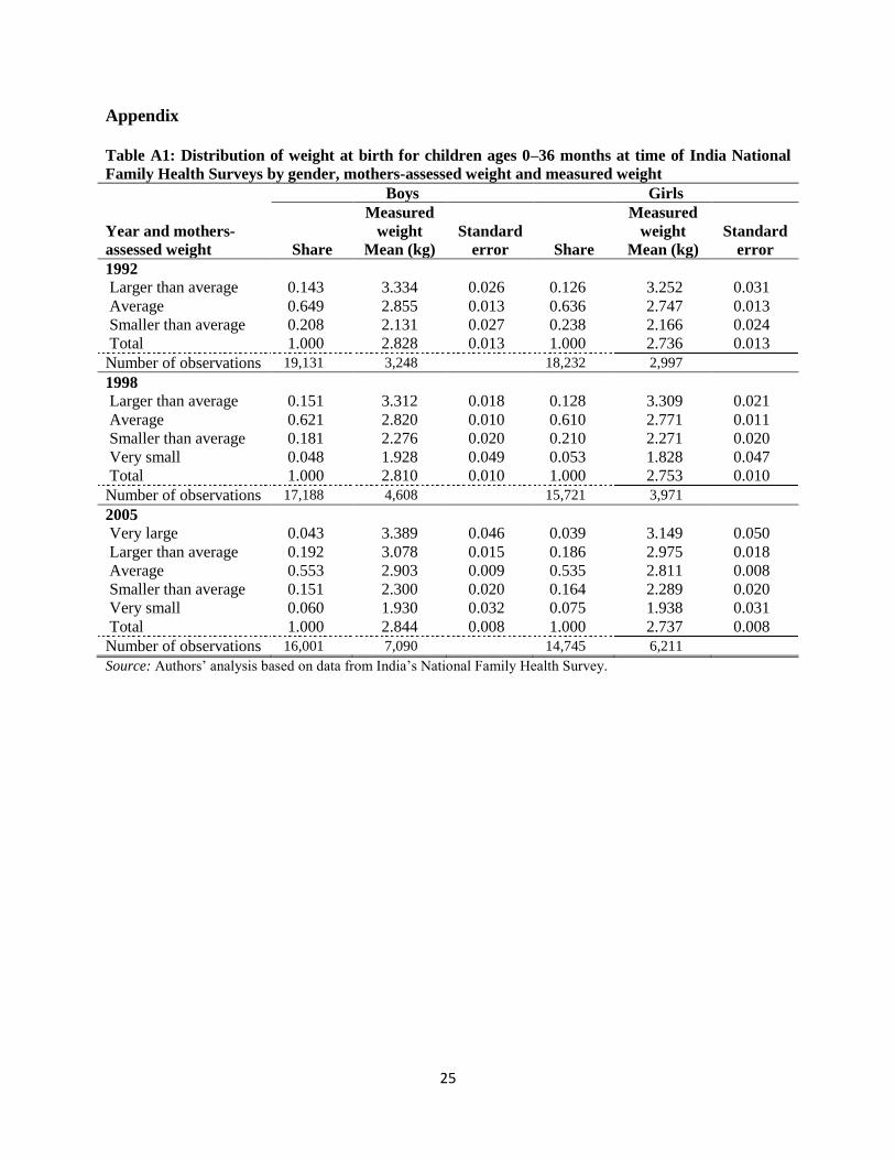
Because children‘s weight at birth influences their health and prospects for

survival (Rosenzweig and Shultz 1982), a key variable for this study is the data on

children‘s weight at birth in the survey. The NFHS collects information on weight at birth

in addition to weight at the time of the survey and asks mothers to categorize the weight

of their children at birth as large, average, or small.6 The sample of children with weight

measured at birth is much smaller than the sample of children whose weight was assessed

by their mother (table A1 in the appendix). The study relies mainly on these subjective

assessments as a proxy for health endowments at birth. The weight of about 20–25

percent of children was lower than average according to their mothers‘ assessments (see

table A1), a figure not out of keeping with the rate of low birth weight children in India.

The data show that average height-for-age has risen over time for both boys and

girls, with z-scores rising from –1.91 in 1992 to –1.55 in 2005 for boys and from –1.86 to

–1.53 for girls. Correspondingly, stunting declined from 72 percent of boys and 70

percent of girls in 1995 to 65 percent for both sexes by 2005. Despite these

improvements, malnutrition remains prevalent in India.

Deaths around the time of birth (neonatal) are high in all rounds of the NFHS

(table 1). Boys accounted for about 56 percent of all deaths in the immediate postnatal

period. However, beyond age 6 months, the share of deaths is higher for girls than for

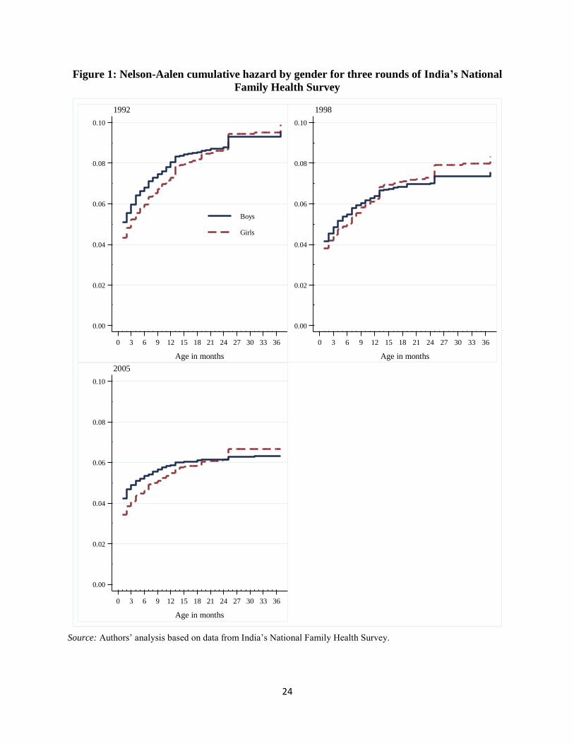
boys. A plot of the cumulative mortality hazard by gender for the three rounds of the

NFHS again shows that more than half the deaths in children under age 36 months occur

in the first month after birth, with little change over the years. It also shows a higher

mortality risk for boys than for girls in the early months of life (figure 1), followed by a

reversal in later months. This switch in mortality patterns results in almost identical total

mortality rates for boys and girls ages 0–36 months.

5 A report by Nutrition Foundation of India concluded that the World Health Organization (WHO) standard

was generally applicable to Indian children (IIPS 2000). The nutritional status of children calculated in this

way is compared with the nutritional status of an international reference population recommended by the

WHO (Dibley and others 1987). The use of this reference group is based on the empirical finding that well-

nourished children in all population groups for which data exist follow similar growth patterns (Martorell

and Habicht 1986). Across rounds of the NFHS, about 10 percent of eligible children were not measured,

either because the children were not at home or because their mothers refused to allow the measurements

(Lokshin, Das Gupta, and Ivaschenko 2005). 6 There is a good correspondence between the measured weight and the weight at birth assessed by the

mothers. For example, in 1992, only about 3 percent of children who were assessed as large at birth had

measured weight in the lowest quintile of the weight distribution. Seidman and others (1987) show that

about 75 percent of self-reported birth weights were accurate within 100 grams. A study by Adegboyea and

Heitmannb (2008) that uses a weight categorization similar to NFHS concludes that maternal assessment of

a child‘s weight at birth ―seems to be sufficiently accurate for clinical and epidemiological use.‖

6

III. Quantifying the Impact of Selective Mortality on Nutritional Indicators

The magnitude of the influence of selective mortality on nutritional status of a population

depends on child mortality level, prevalence of malnutrition among living children, and

prevalence of malnutrition among deceased children (Boerma et al. 1992). Our

population – all children – consists of living and deceased children. Taking a height-for-

age z-score as a measure of malnutrition, the average height-for-age z-score for all

children Zall can be expressed as:

(1) (1 )all s d d dZ Z P Z P ,

where Zs and Zd are average z-scores for survivors and deceased children,

correspondingly, and Pd is the proportion of dead children. The change in the z-score had

deceased children survived is then:

(2)

Assuming that at least some deaths are related to malnutrition (Zd < Zs) the inclusion of

dead children in the sample results in lower average z-scores (Zall < Zs). Δ is larger the

higher is child mortality and the larger is the difference in the average z-scores of living

and deceased children.

The analysis starts with simple simulations illustrating empirically the magnitude

of the potential influence of selective mortality and then moves on to simulations based

on a proportional hazard model.

Simulations Illustrating the Magnitude of Potential Impact of Selective Mortality

What would be the observed height-for-age for all Indian children ages 0–36 months had

the children who died before age 36 months survived? Table 2 presents the simulated

changes in the average height-for-age z-score for different imputation scenarios for three

rounds of NFHS.

The first set of results demonstrates how large the difference in z-scores between

children who died before age 36 months (Zd) and those who survived (Zs) should for Δ in

(2) to be statistically significant. In 1992, 7.7 percent of boys and 8.0 percent of girls died

before age 36 months. The average height-for-age z-score of surviving children (Zs) was

–1.91 with a standard error of 0.016 for boys and –1.86 with a standard error of 0.017 for

girls. The first row of table 2 shows, that imputing a z-score of -2.5 for dead boys results

in the statistically significant changes in overall z-score (Zall) from the actual -1.91 to -

1.95. For girls, the impact of selective mortality would be statistically significant had the

currently deceased girls survived and their average z-score were -2.3.

7

If the average height-for-age of children who died was twice as far below the age

and gender reference mean as that of children who survived (–3.83 rather than –1.91), the

height-for-age z-score for the total sample would rise from –1.91(Zs) to –2.17(Zall), or by

13.5 percent. If a height-for-age z-score of –5.0 (the lower bound recommended as the

cut-off for outliers; WHO 1995) is imputed to a sample of children who died, the overall

z-score would rise from –1.91 to –2.32, or by 21.8 percent. Similar tendencies are

observed for the 1998 and 2005 samples.

The impact of the imputations for height-for-age on the total sample is

proportional to the mortality rates. For example, the imputation of a height-for-age z-

score twice as low as the average to the sample of girls who died before age 36 months

results in a 13.0 percent change in the overall mean z-score in 1992 but only a 8.4 percent

change in 1998 and a 6.6 percent change in 2005, reflecting the decline in girls‘ mortality

rates from 0.077 in 1992 to 0.056 in 2005.

But not all deaths before age 36 months were caused by malnutrition. The next

simulation is based on the results from the literature that estimates the contribution of

malnutrition to child mortality. Puffer and Serrano (1973) found that malnutrition was an

underlying cause in 54 percent of deaths for children ages 2–4 years. Pelletier (1994)

explored 28 prospective datasets and found that the population-attributable risk of

mortality associated with anthropometric deficits varied from 17 percent to 74 percent in

eight studies for Asia and Africa. Pelletier and others (1994) applied to prospective

surveys in Ethiopia, Guatemala, India, and Malawi a new methodology for determining

the association of malnutrition and mortality by the severity of malnutrition. They

demonstrated that 42–57 percent of deaths of children ages 6–59 months were associated

with malnutrition‘s potentiating effects on infectious disease, 76–89 percent of them

attributable to mild to moderate malnutrition. Analysis of data for 53 developing

countries for the 1980s found that about 56 percent of child deaths were associated with

malnutrition. The proportion is close to 67 percent for India, with 73–74 percent of it

attributable to mild to moderate malnutrition (Pelletier and others 1995).

While this approach is based on weight for age and not height-for-age, it makes a

good starting point for a simulation of imputed height-for-age, based on the assumption

that 67 percent of deaths in children up to age 36 months in India were related to

malnutrition (the upper bound for that association; see bottom panel of table 2). The

height-for-age of living children by gender in a particular year was used to impute the

average height-for-age of children whose deaths were not associated with malnutrition.

Of deaths among children related to malnutrition, 70 percent were assumed to have

occurred among children with moderate to mild malnutrition, and an average height to

8

age z-score of –2.5 was imputed to them. For the rest of the sample of children who had

died, an average height to age z-score of –4 was imputed7.

Even though these imputations are based on the upper bound estimates of Pelletier

and others (1995), they result in only modest changes in the overall mean. The largest

changes are observed for the 1992 sample because mortality rates are highest in that year

(see bottom panel of table 2). Had all the children who died survived, the total mean

height-for-age z-score for boys would change from –1.91 to –2.01, a 4.9 percent change.

The impact of imputations is smaller for 1998, at 3.6 percent and 2005, at 4.1 percent.

For girls, the imputations change the total mean from –1.86 to –1.95 in 1992, a 5.1

percent change, and by 3.3 percent for 1998 and 4.09 percent for 2005. The change in

height-for-age z-score is slightly larger in percentage terms in 2005 than in 1998

(although the absolute value of the change is smaller) in keeping with the lower mortality

rate.

Recent studies by Pelletier and Frongillo (2003) and Black and other (2008)

indicate that globally among children younger than 36 months the proportion of deaths

associated with malnutrition declined to 37 percent in the late 1990s and early 2000s

because of the effect of expanded coverage of immunizations, oral rehydration therapy,

antibiotics, and other child survival interventions. Imputations of height-for-age z-scores

corrected for contemporaneous mortality selection based on these estimates would yield

smaller and statistically insignificant changes in the total mean for the 1998 and 2005

NFHS samples. While these more modest associations are not illustrated in table 2, the

simulations that are shown demonstrate that the selectivity mortality would only have a

large impact on observed anthropometrics if there were very large differences in

anthropometrics between the children who died and those who survived. Current research

on the association between mortality and malnutrition does not substantiate such large

differences.

Simulations Based on a Proportional Hazard Model

The simulations discussed in the previous section were based on imputations of a few

categories of height-for-age data to the children in the sample who had died. It is more

realistic to assume that children‘s anthropometrics and survival depend on their

individual characteristics, prenatal conditions, health of the mother, and those of their

household (Wolpin 1997). To approximate this, children who died were matched with

children who survived past the age of 36 months using the estimated survival hazard as a

matching score. The anthropometric scores of children who survived were then imputed

7 Boerma et al (1992) demonstrate that the differences in malnutrition between the children who died after

the measurement and who survived a specified time period in longitudinal studies in Indian states of Tamil

Nadu and Punjab were relatively small: height-for-age z-scores of 60 percent of dead children were lower

than -2 SD from the mean compared to 50 percent among survivors.

9

to the children who had died, and the impact of these imputations on the average height-

for-age z-score of the total sample was estimated.

The estimation uses a standard theoretical framework of household utility

maximization that incorporates the production function of a child‘s health (Behrman and

Deolalikar 1988). Household utility is a function of the consumption and leisure of

household members and the quality (health) and quantity of their children. A household

maximizes its utility subject to budget constraints and the restrictions imposed by the

health production function. The household demand for child health at time t depends on a

set of exogenous characteristics of the child and its mother, household, and community,

as well as some unobserved factors captured by the random error term it (Thomas,

Strauss, and Henriques 1991). This relation can be expressed, in linear form, as:

(3) it it itH X

where vectoriX combines the child‘s, mother‘s, household‘s, and community‘s

characteristics, and β is a vector of parameters.

The child‘s health can be linked to mortality through the stochastic rule for

observing death (Sickles and Taubman 1997). The mortality state for child i at time t is

defined as:

(4)

*1

0

it it itM if H H

otherwise

where *

itH is a child- and time-specific mortality threshold that can be interpreted as a

shock whose arrival time follows a Poisson distribution. The probability that a shock *

itH

occurs during the period ( , )t t is 0( ) ( )P h t o . Then the hazard of dying during

this period is:

(5) 0( ) ( )[1 ( )]i ith t h t F H

where h0(t) is the baseline hazard and F(Hit) is the health distribution function. The

survival function is then:

(6) 0( | ) exp{ ( )[1 ( )] }.i i itS t x h t F H t

Assumptions about the distribution of the health shocks that are standard in the

literature on mortality can be used to estimate the survival function using the Weibull

proportion hazard model, such that:

(7)

1 1

1

( ) exp{ } exp{ }

( | ) exp{ exp( ) }

i it i

i i

h t t H t x

and

S t x t x t

10

where θ is an unknown parameter.

To control for the unobserved heterogeneity in children‘s health (frailty), a

parameter is introduced that represents the effect of unobserved factors on survival. This

effect is not directly estimated from data but is assumed to have unit mean and variance

αi that is estimated (see Vaupel, Manton, and Stallard 1979; Lancaster 1979; Hougaard

1995). In the presence of such unobserved heterogeneity, survival function (7) becomes:

(8) ( | , ) { ( | )} i

i i iS t x S t x .

The unconditional survival function is obtained by integrating out the

unobservable factor by assuming a distribution for α. If the unobserved factor is inverse-

Gaussian-distributed,8 the survival function of the Weibull proportional hazard model (8)

becomes:

(9) 1/21 [1 2 ln( ( ))]

( | , ) exp{ }i

S tS t x

.

The parameters of equation (9) are estimated using the maximum likelihood algorithm.

Once these parameters are obtained, dead and surviving children can be matched on the

estimated hazard as a matching score, and this matching can be used to impute a height-

for-age z-score for children who died. The matching approach used here is analogous to

the approach used in propensity score matching (see Rubin 1973, 1979; Rosenbaum and

Rubin 1983), but the hazard function is a different functional form than commonly used

for propensity score matching. It was chosen for its ability to account for censoring and

truncation, making it the preferred model for estimating survival.9 The overall conclusion

is robust to an estimation of survival based on a probit regression (results not reported in

tables), the functional form more commonly employed in propensity score matching.

IV. Results

The explanatory variables used in proportional hazard estimation (equation 7) include the

child‘s sex, birth order, and weight at birth; the mother‘s age, educational attainment,

employment status, and other characteristics; household size, socio-demographic

8 For the inverse-Gaussian frailty distribution, the relative variability of frailties among surviving children

decreases with age, which could be a more realistic assumption for modeling child mortality; Gamma

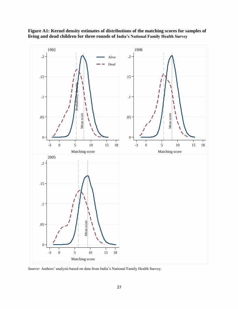
frailty distribution assumes constant variability of frailty with age (Gutierrez 2002). 9 Samples of dead and surviving children were matched using a nearest neighbor algorithm with the

restriction that observations in both samples are on a common support in terms of the matching score

(Heckman, LaLonde, and Smith 1999). The probability density functions of matching scores for dead and

surviving children are shown in figure A1 in the appendix. An alternative, and probably more intuitive, way

to run these simulations would be to model children‘s height for age z-scores as a function of their

characteristics and to impute height for age z-scores to the dead children using out-of-sample prediction.

The approach here is similar to that because the out-of-sample prediction could be interpreted as a case of

matching. The advantages of the current approach are the use of a more flexible function form for the

matching and the ability of the hazard model to deal better with attrition issues.

11

composition, wealth index, religion, and caste; and the availability of community services

and infrastructure. The descriptive statistics for these variables are presented in table 3.

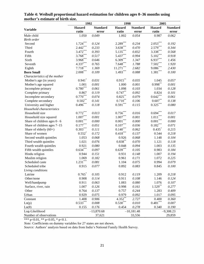
Tables 4 and 5 show the coefficients of the Weibull proportional hazard

estimation for children younger than age 36 months using three rounds of the NFHS.10

Table 4 includes the child‘s weight at birth estimated by the mother; Table 5 uses weight

measured at birth. The weight at birth is one of the important factors affecting neo-natal

child mortality that combines the unobserved information about pre-natal conditions and

shocks experienced by the mother and her child (i.e., Claeson, et al. 2000). The results of

the two estimations are not directly comparable as one is a categorical variable (mother‘s

assessment of weight at birth) and the other is a continuous variable (measured weight),

but the implications are similar11

. The remainder of the discussion focuses on the

estimations based on the specification using mother-assessed weight at birth because the

sample sizes are much larger.

The estimated hazard odds ratios on the control variables in the estimations of

proportional hazard models reveal the expected relationship between child mortality and

characteristics of the child, mother, and household. A child‘s gender has no effect on

mortality hazard: mortality rates for boys are higher than for girls in the six months after

birth and lower after that. A higher birth order has a negative impact on survival

probabilities (Miller et al. 1992). Weight at birth, whether assessed by the mother or

measured at birth, is a strong predictor of mortality. Children whose mother‘s assessed

their weight as small (with an odds ratio greater than 1 on the dummy variable reported in

table 4) and children with low measured weight (with odds ratios less than one on the

continuous measured weight variables in table 6) are significantly less likely to survive

than are children who weigh more at birth.

Children living in the wealthiest households and with better educated mothers

have better prospects for survival than do children from poor households and with less

educated mothers. In an inverted U-shaped relationship, children‘s survival improves

with the mother‘s age till about age 40 and declines thereafter.

10

The specification with Weibull distribution is selected based on the comparison of Akaike (1974)

information criterion values for specifications with exponential, Weibull, Gompertz, log-normal, log-

logistic, and general gamma distributions. 11

Note that the interpretation of the numbers presented in tables 5 and 6 are different from the standard

interpretation of the regression coefficients. The odds ratios are always positive; odds ratios that are less

than one indicate that an increase in a particular factor reduces the probability of an event, while odds ratios

greater than 1 mean that a particular factor increases the probability of an event. Correspondingly, the t-

tests of the odds ratio test the null hypothesis of odds ratios being equal to 1. For comparability, we re-

estimated the hazard model shown in Table 5 with the continuous variable on weight at birth categorized as

a binary indicator equal to 1 for children with weight at birth < 2,500 grams. The odds ratio for this dummy

is less than 1 and significant, but the effect of being born with low weight is smaller compared to

coefficient in Table 5. One explanation for this could be that children whose weight was measured at birth

come from the wealthier families with better access to post-natal health care.

12

Table 6 presents the simulated impact of the matched imputations of height-for-

age z-scores for all children ages 0–36 month who did not survive till the age of 36

months. The average z-score is higher for children with measured weight at birth than for

children with mother-assessed weights at birth reflecting wealth differences.

In 1992, the average height-for-age z-score for boys who survived past age 36

months was –1.913. When the matched z-score estimates are imputed to children who

died before age 36 months, the overall average height-for-age z-score becomes –1.936;

the difference of –0.023 is not statistically significantly different from 0. Similar

differences are observed for other years. In all years, for both boys and girls, the

imputations have no significant impact on the overall anthropometric indices. In all cases,

the average imputed height-for-age z-score in the simulations based on the survival

model is smaller than the imputed z-score that would result in a statistically significant

change in the overall height-for-age z-score as shown in first panel of table 212

. These

results resonate with other studies that use longitudinal data from surviving and non-

surviving children and find a modest amount of selection via child mortality on height-

for-age z-scores i.e., Boerma et al (1992), Moradi (2010)13

.

The effect of the change in mortality on gender patterns of height-for-age z-scores

was also simulated using the results of hazard function estimations. This simulation

closes the gender gap in mortality in the age 3–36 month group by artificially increasing

the mortality among boys14

. The simulation assumes that 144 of the boys in the sample

with the lowest probabilities of survival did not survive and thus did not contribute to the

observed height-for-age z-scores. The simulation of this increase in boys‘ mortality on

the data from 1992 of NFHS demonstrates a 0.12 percent increase in the height-for-age z-

score. This clearly has a negligible impact on the difference in nutritional status between

boys and girls.

Finally, taking our model a step further, we simulate the health outcomes of

Indian children if the mortality rates in India were as high as one of the highest rates

current in Africa. In this simulation we change the surviving status of living children with

lowest probabilities of survival to reach the mortality rate of 15 percent for both boys and

12

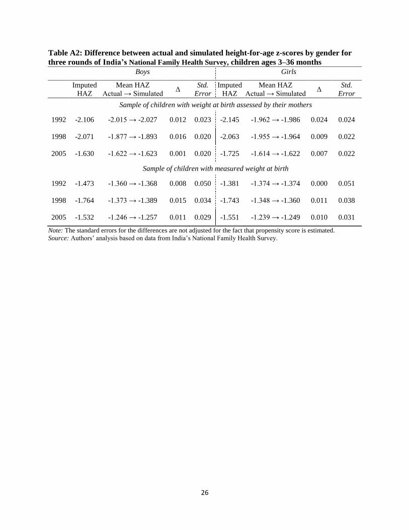
Table A2 in Appendix presents the simulated impact of the matched imputations of height-for-age z-

scores for children ages 3–36 months who did not survive till the age of 36 months. Neonatal mortality was

excluded in the hazard estimates as it could have a different set of correlates, but the results are not

particularly sensitive to the exclusion of this age group. 13

Our empirical model fails to account for the possible selection bias due to high levels of maternal

mortality in India (e.g., Ronsmans and Graham 2006). Correction of this bias would increase the gap in

anthropometric outcomes between the deceased and living children. Unfortunately, the nature of IFHS

sample makes it difficult to look on the relationship of maternal mortality and children health outcomes. 14

In principle, one could, simulate a more desirable decrease in girls‘ mortality to close this gap, but it is

more direct to use the estimates from boys actually in the sample then to make projections for girls who

would otherwise have been in the sample.

13

girls.15

The results of the simulation (table 7) show only minor changes in the aggregate

height-for-age z-scores when the mortality rates are increased from 5 – 8 percent (table 1)

to 15 percent. The changes are statistically significant for the samples of boys and girls in

1998 and for the sample of boys in 2005, but even in these cases the magnitudes of the

changes have not exceeded 3 percent.

V. Conclusion

This paper used data from three rounds of a nationally representative health survey in

India to assess the magnitude of the bias in children‘s anthropometrics due to selective

mortality. The nutritional status of the child population was simulated under the

counterfactual scenario that all children who had died in the first three years of life were

alive at the time of measurement. These simulations imputed various values of height-

for-age z-scores to the sample of dead children. The simple simulations, with imputed z-

scores that are independent of the child‘s characteristics, show that, at the rates of child

mortality prevailing in India in 1992–2005, the selective mortality could have only a

moderate impact on overall anthropometric measures. The imputations based on the

literature on the association between child mortality and nutrition result in only a 5

percent difference between the counterfactual and the actual height-for-age z-scores.

The simulations based on the hazard model that takes into account differences in

mortality and anthropometrics related to child characteristics are consistent with the

observation that malnourished children are less likely to survive and thus to contribute to

anthropomorphic measurements. However, the results also show that with the current low

(and declining) mortality rates by historical standards, improved survival rates have an

insignificant impact on overall height-for-age z-scores. The changes in mortality between

1992 and 2005 imply that some malnourished children who would previously have died

instead survived and are measured in the 2005 survey. To the degree that selective

mortality affects overall malnutrition levels or rates, the reductions in child mortality

mask some of the improvement in nutrition. However, the results of this study suggest

that progress on the fourth Millennium Development Goal to reduce child mortality only

lightly obscures the results for the target for the first Millennium Development Goal to

reduce malnutrition and hunger.16

Similarly, the findings imply that differences in mortality are unlikely to explain

gender differences in anthropometrics—or their absence. While the NFHS data do not

15

This rate corresponds to the high mortality rate of 14.2 percent observed among boys in Cote d‘Ivoire in

1998. The rate for Cote D‘Ivoire was the highest mortality rate from 30 DHS of African countries

reviewed. 16 This target is measured in terms of underweight rather than height for age. Underweight is somewhat

easier to measure in a survey covering young children, though height for age is a clearer indicator of

cumulative health. While underweight rates and stunting rates often differ, trends in the two tend to move

together.

14

show a marked gender pattern in overall mortality of children 0–36 months, deaths are

higher for girls after the neonatal period. Nevertheless, the imputations here have no

significant impact on relative nutritional status. While the results reported here are from

India over a two decade period, in a more general sense, it appears that selective

mortality is unlikely to be of significant magnitude in most countries to have a large

impact on trends in populations or subpopulations.

15

References

Adegboye, A., and B. Heitmannb. 2008 ―Accuracy and correlates of maternal recall of

birth weight and gestational age.‖ International Journal of Obstetrics and

Gynaecology 115 (7): 866–93

Alderman, H., Behrman, J. and J. Hoddinott. 2005. ―Nutrition, malnutrition, and

economic growth.‖ In Health and economic growth: findings and policy

implications, ed. Guillem López-Casasnovas, Berta Rivera, and Luis Currais.

Cambridge, Mass: MIT Press.

Almond, D. and J. Currie (2010) ―Human Capital Development before Age Five,‖ NBER

Working Paper Series, Working Paper #15827

Behrman, J., and A. Deolalikar (1988) ―Health and nutrition.‖ In Handbook of

development economics, Vol. 1, ed. H. Chenery and T. Srinivasan. Amsterdam:

North Holland.

Black, R., L. Allen, Z. Bhutta, L. Caulfi, M. Onis, M. Ezzati, C. Mathers, and J. Rivera.

2008. ―Maternal and child undernutrition: global and regional exposures and

health consequences.‖ Lancet 371: 243–60.

Boerma, J., Sommerfelt, E., and G. Bicego. 1992. ―Child Anthropometry in Cross-

Sectional Surveys in Developing Countries: an Assessment of the Survivor Bias,‖

American Journal of Epidemiology, Vol. 135(4): 438–49

Bozzoli, C., Deaton, A., and C. Quintanta-Domeque. 2007. ―Adult Height and Childhood

Mortality.‖ Demography, Vol. 46(4): 647–69

Claeson, M., Bos, E., Mawji, T. and I. Pathmanathan (2000) ―Reducing child mortality in

India in the new millennium.‖ Bulletin of the World Health Organization, Vol.

78: 1192-1199

Dancer, D., Rammohan, A., and M. Smith. 2008. ―Infant mortality and child nutrition in

Bangladesh.‖ Health Economics 17: 1015–35.

Deaton, A. 2007. ―Height, health and development.‖ Proceeding of the National

Academy of Science 104 (33): 13232–37.

Dibley, M., J. Goldsby, N. Staehling, and F. Trowbridge. 1987. ―Development of

normalized curves for the international growth reference: historical and technical

considerations.‖ American Journal of Clinical Nutrition 46: 736–48.

Filmer, D. and L. Pritchett. 2001. ―Estimating wealth effects without expenditure data—

or tears: an application to educational enrollments in states of India.‖

Demography 38 (1): 115–32.

Fitzgerald, J., P. Gottschalk, and R. Moffitt. 1998. ―An analysis of sample attrition in

panel data.‖ Journal of Human Resources 33: 251–99.

Fogel, Robert W. 2004. ―Health, nutrition, and economic growth.‖ Economic

Development & Cultural Change 52 (3): 643–58.

16

Gørgens, T., Meng, X. and R. Vaithianathan. 2007. ―Stunting and Selection Effects of

Famine: A Case Study of the Great Chinese Famine.‖ IZA Discussion Paper No.

2543. Institute for the Study of Labor, Bonn, Germany.

Gutierrez, R. 2002. ―Parametric frailty and shared frailty survival models.‖ Stata Journal

2 (1): 22–44.

Heckman, J., R. LaLonde, and J. Smith. 1999. ―The economics and econometrics of

active labor market programs.‖ In Handbook of labor economics, Vol.III, ed. O.

Ashenfelter and D. Card. Amsterdam: Elsevier.

Hougaard, P. 1995. ―Frailty models for survival data.‖ Lifetime Data Analysis 1: 255–73

Lancaster, T. 1979. ―Econometric methods for the duration of unemployment.‖

Econometrica, 47: 939–56

Lokshin, M., Das Gupta, M., and O. Ivaschenko. 2005. ―An assessment of India's

Integrated Child Development Services Nutrition Program.‖ Development and

Change 36 (4): 613–40.

Maccini, Sharon and Dean Yang (2009). Under the Weather: Health, Schooling, and

Economic Consequences of Early-Life Rainfall. American Economic Review. June

99 (3), 1006-26.

Martorell, R. and J. Habicht. 1986. ―Growth in early childhood in developing countries.‖

In Falkner, F. and J. Tanner (eds): Human Growth. Volume 3. Methodology.

Ecological, Genetic, and Nutritional Effects on Growth. Second Edition. New

York: Plenum, pp. 241-262.

Miller, J., Trussel, J., Pebley, A., and B. Vaughan. 1992. ―Birth spacing and child

mortality in Bangladesh and the Philippines.‖ Demography 29: 305–18.

Moradi, A. 2010. ―Selective mortality or growth after childhood? What really is Key to

understand the Puzzlingly Tall Adult Heights in Sub-Saharan Africa". CSAE

WPS 2010-17

Pelletier, D. 1994. ―Relationship between child anthropometry and the mortality in

developing countries: implications for policy programs and future research.‖

Journal of Nutrition, 124 (10): 2047S–81S.

Pelletier, D., and E. Frognillo. 2003. ―Change in child survival are strongly associated

with changes in malnutrition in developing countries.‖ Journal of Nutrition 133:

107–19.

Pelletier, D., A. Frongillo, D. Schroeder, and J. Habicht. 1994. ―A methodology for

estimating the contribution of malnutrition to child mortality in developing

countries.‖ Journal of Nutrition 124 (10): 2106S–22S

Pelletier, D., E. Frognillo, D. Schroeder, and J. Habicht. 1995. ―The effects of

malnutrition on child mortality in developing countries.‖ Bulletin of the World

Health Organization 73 (4): 443–46.

Pitt, Mark. 1997. ―Estimating the determinants of child health when fertility and

mortality are selective.‖ Journal of Human Resources 32 (1): 129–58.

17

Puffer, R., and C. Serrano. 1973. Patterns of mortality in childhood. Scientific

Publication 262. Washington, DC: Pan American Health Organization.

Ronsmans, C., and W. Graham. 2006. ―Maternal mortality: who, when, where,

and why.‖ Lancet, Vol. 368: 1189-200

Rosenzweig, M., and T. Schultz. 1982. ―The behavior of mothers as inputs to child

health: the determinants of birth weight, gestation, and rate of fetal growth.‖ In

Economic aspects of health ed. V. Fuchs. Chicago: University of Chicago Press,

Chicago.

Rosenbaum, P., and D. Rubin. 1983. ―The central role of the propensity score in

observational studies for causal effects.‖ Biometrika 70 (1): 41–55.

Rubin, D. 1973. ―Matching to remove bias in observational studies.‖ Biometrics 29: 159–

83.

________, 1979 ―Using multivariate matched sampling and regression adjustment to

control bias in observation studies.‖ Journal of the American Statistical

Association 74 (366): 318–28.

Rutstein, S., and K. Johnson. 2004. ―The DHS wealth index.‖ DHS Comparative Reports.

6., Calverton, Maryland: ORC Macro.

Seidman, D., P. Slater, P. Ever-Hadani, and R. Gale. 1987. ―Accuracy of mothers' recall

of birthweight and gestational age.‖ International Journal of Obstetrics &

Gynaecology 94 (8): 731–35.

Shrimpton R, C. Victora, M. de Onis, R. Costa Lima, M. Blössner, and G. Clugston.

2001. ―Worldwide timing of growth faltering: implications for nutritional

interventions.‖ Pediatrics 107: 75-81.

Sickles R., and P. Taubman. 1997. ―Mortality and morbidity among adults and elderly.‖

in Handbook of population and family economics, Vol. 1A, ed. M. Rosenzweig

and O. Stark. Amsterdam: North-Holland.

Steckel, Richard H. 1995. ―Stature and the standard of living.‖ Journal of Economic

Literature 33 (4): 1903–40.

———. 2009. ―Heights and human welfare: recent developments and new directions.”

Explorations in Economic History 46 (1): 1–23.

Thomas, D., J. Strauss, and M. Henriques. 1991. ―How does mother's education affect

child height?‖ Journal of Human Resources 26 (2): 183–211.

Victora, C., L. Adair, C. Fall, P. Hallal, R. Martorell, L. Richter, and H. Sachdev. 2008.

―Maternal and Child Undernutrition Study Group. Maternal and child

undernutrition: consequences for adult health and human capital.‖ Lancet 371

(9609): 302.

Victora, C, M. de Onis, P. Hallal, M. Blossner and R. Shrimpton. 2010. Worldwide

timing of Growth Faltering: Revisiting Implications for Interventions. Pediatrics.

125: 473-480..

Vaupel, J., K. Manton, and E. Stallard. 1979. ―The impact of heterogeneity in individual

frailty on the dynamics of mortality.‖ Demography 16: 439–54.

18

Wolpin, K. 1997. ―Determinants and consequences of the mortality and health of infants

and children.‖ In Handbook of population and family economics, Vol. 1A, ed. M.

Rosenzweig and O. Stark. Amsterdam: North-Holland.

WHO (World Health Organization). 1995. Physical status: the use and interpretation of

anthropometry. WHO technical report series 854. Geneva: World Health

Organization.

———. 2006. ―Child growth standards: length/height-for-age, weight-for-age, weight-

for-length, weight-for-height and body mass index-for-age: methods and

development.‖ Geneva: World Health Organization.

19

Table 1: Proportion of total deaths by age and gender for three rounds of India’s

National Family Health Survey (percent)

1992 1998 2005

Age Boys Girls Boys Girls Boys Girls

Neonatal 50.7 40.6 53.75 44.0 56.9 47.3

0–6 months 19.7 20.7 18.9 19.4 18.6 19.6

7–12 months 14.2 17. 8 12. 5 16.2 10.9 14.5

13–18 months 2.2 2.7 2.0 2.6 1.7 2.3

19–24 months 8.4 11.6 8.2 11.5 7.4 10.6

25–36 months 4.9 6.6 4.7 6.3 4.5 5.6

Total 100 100 100 100 100 100

Mortality rate

Standard error 0.080

(0.001)

0.077

(0.001)

0.064

(0.001)

0.066

(0.002)

0.058

(0.002)

0.056

(0.002)

Source: Authors‘ analysis based on data from India‘s National Family Health Survey.

Table 2: Changes in the total mean height-for-age z-score (HAZ) for different

imputation scenarios.

Boys Girls

Imputed

HAZ

Zd

Mean HAZ

Actual → Simulated

Zs → Zall

%Δ

total

HAZ

Imputed

HAZ

Zd

Mean HAZ

Actual → Simulated

Zs → Zall

%Δ

total

HAZ

Imputed HAZ (Zd) that results in a statistically significant change in total HAZ (Zall)

1992 -2.15 -1.91 → -1.95 1.70 -2.13 -1.86 → -1.90 1.85

1998 -2.12 -1.77 → -1.80 1.58 -2.22 -1.85 → -1.88 1.65

2005 -1.95 -1.55 → -1.57 1.77 -1.98 -1.53 → -1.56 1.92

Imputed HAZ (Zd) is twice as low as the average observed HAZ (Zs)

1992 -3.83 -1.91 → -2.17 13.51 -3.72 -1.86 → -2.10 12.99

1998 -3.55 -1.77 → -1.92 8.12 -3.71 -1.85 → -2.01 8.37

2005 -3.09 -1.55 → -1.65 6.78 -3.06 -1.53 → -1.63 6.60

Imputed HAZ (Zd) = - 5SD

1992 -5.00 -1.91 → -2.33 21.81 -5.00 -1.86 → -2.27 21.90

1998 -5.00 -1.77 → -2.03 14.78 -5.00 -1.85 → -2.12 14.21

2005 -5.00 -1.55 → -1.78 15.13 -5.00 -1.53 → -1.76 14.95

HAZ imputed based on upper bounds of Pelletier et al. (1995) estimates

1992 -2.61 -1.91 → -2.01 4.91 -2.59 -1.86 → -1.95 5.09

1998 -2.56 -1.77 → -1.84 3.61 -2.59 -1.85 → -1.92 3.32

2005 -2.49 -1.55 → -1.61 4.12 -2.48 -1.53 → -1.59 4.09

Source: Authors‘ analysis based on data from India‘s National Family Health Survey and estimates from

Pelletier and others (1995) on the upper bound of deaths in children due to malnutrition.

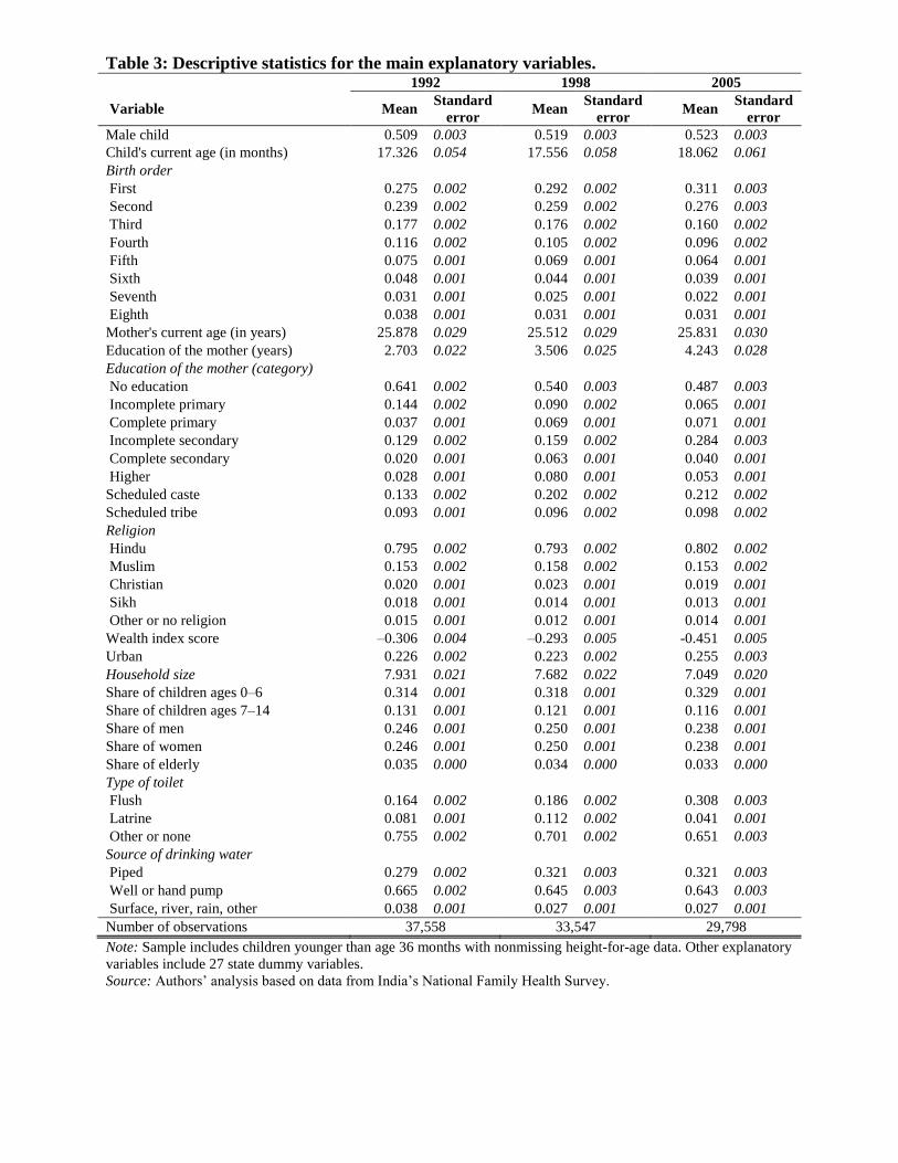
Table 3: Descriptive statistics for the main explanatory variables. 1992 1998 2005

Variable Mean Standard

error Mean

Standard

error Mean

Standard

error

Male child 0.509 0.003 0.519 0.003 0.523 0.003

Child's current age (in months) 17.326 0.054 17.556 0.058 18.062 0.061

Birth order

First 0.275 0.002 0.292 0.002 0.311 0.003

Second 0.239 0.002 0.259 0.002 0.276 0.003

Third 0.177 0.002 0.176 0.002 0.160 0.002

Fourth 0.116 0.002 0.105 0.002 0.096 0.002

Fifth 0.075 0.001 0.069 0.001 0.064 0.001

Sixth 0.048 0.001 0.044 0.001 0.039 0.001

Seventh 0.031 0.001 0.025 0.001 0.022 0.001

Eighth 0.038 0.001 0.031 0.001 0.031 0.001

Mother's current age (in years) 25.878 0.029 25.512 0.029 25.831 0.030

Education of the mother (years) 2.703 0.022 3.506 0.025 4.243 0.028

Education of the mother (category)

No education 0.641 0.002 0.540 0.003 0.487 0.003

Incomplete primary 0.144 0.002 0.090 0.002 0.065 0.001

Complete primary 0.037 0.001 0.069 0.001 0.071 0.001

Incomplete secondary 0.129 0.002 0.159 0.002 0.284 0.003

Complete secondary 0.020 0.001 0.063 0.001 0.040 0.001

Higher 0.028 0.001 0.080 0.001 0.053 0.001

Scheduled caste 0.133 0.002 0.202 0.002 0.212 0.002

Scheduled tribe 0.093 0.001 0.096 0.002 0.098 0.002

Religion

Hindu 0.795 0.002 0.793 0.002 0.802 0.002

Muslim 0.153 0.002 0.158 0.002 0.153 0.002

Christian 0.020 0.001 0.023 0.001 0.019 0.001

Sikh 0.018 0.001 0.014 0.001 0.013 0.001

Other or no religion 0.015 0.001 0.012 0.001 0.014 0.001

Wealth index score –0.306 0.004 –0.293 0.005 -0.451 0.005

Urban 0.226 0.002 0.223 0.002 0.255 0.003

Household size 7.931 0.021 7.682 0.022 7.049 0.020

Share of children ages 0–6 0.314 0.001 0.318 0.001 0.329 0.001

Share of children ages 7–14 0.131 0.001 0.121 0.001 0.116 0.001

Share of men 0.246 0.001 0.250 0.001 0.238 0.001

Share of women 0.246 0.001 0.250 0.001 0.238 0.001

Share of elderly 0.035 0.000 0.034 0.000 0.033 0.000

Type of toilet

Flush 0.164 0.002 0.186 0.002 0.308 0.003

Latrine 0.081 0.001 0.112 0.002 0.041 0.001

Other or none 0.755 0.002 0.701 0.002 0.651 0.003

Source of drinking water

Piped 0.279 0.002 0.321 0.003 0.321 0.003

Well or hand pump 0.665 0.002 0.645 0.003 0.643 0.003

Surface, river, rain, other 0.038 0.001 0.027 0.001 0.027 0.001

Number of observations 37,558 33,547 29,798

Note: Sample includes children younger than age 36 months with nonmissing height-for-age data. Other explanatory

variables include 27 state dummy variables.

Source: Authors‘ analysis based on data from India‘s National Family Health Survey.

21

Table 4: Weibull proportional hazard estimation for children ages 0–36 months using

mother’s estimate of birth size.

1992 1998 2005

Variable Hazard

ratio

Standard

error

Hazard

ratio

Standard

error

Hazard

ratio

Standard

error

Male child 1.050 0.049 1.002 0.054 0.987 0.062

Birth order

Second 1.724***

0.124 2.289***

0.234 2.053***

0.192

Third 2.442***

0.233 3.638***

0.470 2.579***

0.344

Fourth 3.472***

0.393 5.135***

0.832 3.338***

0.568

Fifth 3.768***

0.517 5.437***

0.994 5.102***

0.918

Sixth 3.968***

0.646 6.309***

1.347 6.937***

1.456

Seventh 4.337***

0.765 7.648***

1.788 7.502***

1.920

Eighth 7.718***

1.369 11.271***

2.682 9.086***

2.430

Born Small 2.008***

0.109 1.493***

0.088 1.381***

0.100

Characteristics of the mother

Mother's age (in years) 0.941* 0.031 0.915

** 0.035 1.045 0.057

Mother's age squared 1.001 0.001 1.000 0.001 0.998**

0.001

Incomplete primary 0.780***

0.061 1.098 0.103 1.034 0.128

Complete primary 0.867 0.119 0.747**

0.092 0.824 0.101

Incomplete secondary 0.770***

0.074 0.825**

0.079 0.642***

0.061

Complete secondary 0.502**

0.141 0.710**

0.106 0.607**

0.138

University and higher 0.496***

0.118 0.591***

0.115 0.325***

0.080

Household characteristics

Household size 0.772***

0.013 0.756***

0.016 0.694***

0.017

Household size squared 1.007***

0.001 1.007***

0.001 1.011***

0.001

Share of children ages 0– 6

years

0.001***

0.000 0.001***

0.000 0.001***

0.000

Share of children ages 7–15

years 0.177

*** 0.051 0.107

*** 0.036 0.182

*** 0.071

Share of elderly (60+) 0.303***

0.111 0.140***

0.062 0.435* 0.215

Share of women 0.552* 0.172 0.418

*** 0.137 0.544 0.218

Second wealth quintiles 1.053 0.068 0.926 0.068 1.148 0.104

Third wealth quintiles 1.021 0.076 0.838**

0.070 1.121 0.118

Fourth wealth quintiles 0.921 0.080 0.848 0.094 1.003 0.135

Fifth wealth quintiles 0.634***

0.097 0.639***

0.105 0.983 0.184

Hindu religion 0.944 0.151 0.931 0.148 1.007 0.194

Muslim religion 1.069 0.182 0.961 0.171 1.072 0.225

Scheduled caste 1.231***

0.081 1.104 0.075 0.994 0.079

Scheduled tribe 0.915 0.077 0.892 0.083 0.845 0.100

Living conditions

Latrine 0.765* 0.105 0.912 0.119 1.209 0.218

Other/none 0.908 0.114 0.911 0.108 1.146 0.124

Well/handpump 0.911 0.063 1.083 0.080 1.076 0.107

Surface, river, rain 1.007 0.126 0.998 0.161 1.529**

0.277

Other 0.764 0.137 0.757 0.244 1.283 0.409

Urban 0.929 0.075 0.979 0.092 1.017 0.095

Constant 1.408 0.906 4.352**

2.727 0.400 0.360

Ln(p) 0.533***

0.008 0.530***

0.010 0.481***

0.007

Ln(θ) 0.155 0.176 0.454 0.278 0.340 0.190

Log-Likelihood –13,870.68 –10,181.48 –9,308.23

Number of observations 37,621 33,556 29,859

*** p<0.01, ** p<0.05, * p<0.1.

Note: Coefficients on dummy variables for 27 states are not shown.

Source: Authors‘ analysis based on data from India‘s National Family Health Survey.

22

Table 5: Weibull proportional hazard estimation for children ages 0–36 months using

recorded weights.

1992 1998 2005

Variable Hazard

ratio

Standard

error

Hazard

ratio

Standard

error

Hazard

ratio

Standard

error

Male child 1.588**

0.287 1.181 0.186 1.133 0.168

Birth order

Second 1.967***

0.479 4.476***

0.986 2.983***

0.547

Third 3.994***

1.287 4.205***

1.334 4.367***

1.212

Fourth 7.157***

3.013 4.286***

2.062 9.430***

3.451

Fifth 11.530***

6.806 10.650***

5.736 3.081* 1.946

Sixth 0.000***

0.000 5.201**

3.669 49.997***

26.524

Seventh 1.277 1.473 17.193***

11.702 30.526***

16.715

Eighth 16.028***

13.796 10.887**

12.939 1.214 1.539

Measured weight at birth 0.457***

0.068 0.533***

0.074 0.668***

0.098

Characteristics of the mother

Mother's age (in years) 0.905 0.107 0.905 0.103 1.293* 0.193

Mother's age squared 1.001 0.002 1.001 0.002 0.994**

0.003

Incomplete primary 0.930 0.238 0.821 0.190 1.047 0.257

Complete primary 1.358 0.426 0.533* 0.196 0.763 0.247

Incomplete secondary 0.642 0.182 0.461***

0.105 0.555***

0.104

Complete secondary 0.791 0.324 0.477**

0.141 0.469**

0.147

University and higher 0.512 0.210 0.317***

0.100 0.209***

0.078

Household characteristics

Household size 0.756***

0.046 0.668***

0.038 0.684***

0.042

Household size squared 1.006***

0.001 1.012***

0.002 1.010***

0.003

Share of children ages 0–6 years 0.001***

0.000 0.001***

0.000 0.001***

0.000

Share of children ages 7–15

years 0.063

*** 0.063 0.075

*** 0.070 0.022

*** 0.018

Share of elderly (60+) 0.637 0.741 0.078**

0.092 0.222* 0.194

Share of women 0.467 0.424 0.581 0.484 0.214**

0.150

Second wealth quintiles 0.694 0.320 0.787 0.250 1.147 0.327

Third wealth quintiles 0.653 0.289 0.884 0.271 1.628* 0.426

Fourth wealth quintiles 0.613 0.276 0.872 0.279 1.915**

0.542

Fifth wealth quintiles 0.399* 0.201 1.235 0.454 2.078

** 0.686

Hindu religion 0.835 0.221 1.194 0.348 0.846 0.234

Muslim religion 0.670 0.271 1.011 0.395 0.802 0.287

Scheduled caste 0.663 0.247 1.038 0.218 1.084 0.191

Scheduled tribe 0.426* 0.190 1.011 0.326 0.756 0.232

Living conditions

Latrine 0.819 0.243 0.981 0.280 0.957 0.358

Other/none 1.228 0.325 0.928 0.249 1.344 0.279

Well/handpump 0.938 0.177 0.916 0.158 1.351**

0.194

Surface, river, rain 1.301 0.686 1.154 0.697 1.043 0.559

Other 0.394 0.238 2.168* 0.990 1.342 0.837

Urban 1.546* 0.346 0.888 0.213 1.071 0.184

Constant 22.884* 39.678 55.530

** 100.703 0.339 0.744

Ln(p) 0.547***

0.027 0.517***

0.023 0.522***

0.018

Ln(θ) 0.001***

0.000 0.001***

0.000 0.001***

0.000

Log-Likelihood –1,011.30 –1,239.06 –1,791.04

Number of observations 6,228 8,555 12,755

***p<0.01, **p<0.05, *p<0.1.

Note: Coefficients on dummy variables for 27 states are not shown.

Source: Authors‘ analysis based on data from India‘s National Family Health Survey

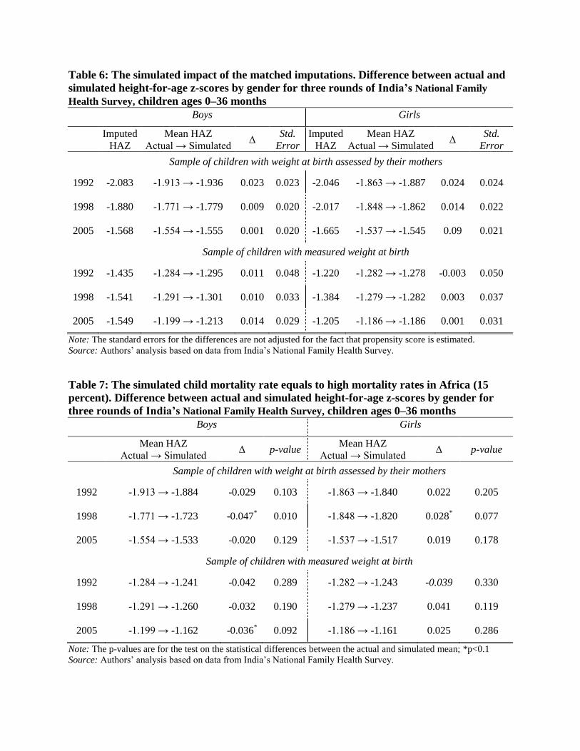
Table 6: The simulated impact of the matched imputations. Difference between actual and

simulated height-for-age z-scores by gender for three rounds of India’s National Family

Health Survey, children ages 0–36 months

Boys Girls

Imputed

HAZ

Mean HAZ

Actual → Simulated Δ

Std.

Error

Imputed

HAZ

Mean HAZ

Actual → Simulated Δ

Std.

Error

Sample of children with weight at birth assessed by their mothers

1992 -2.083 -1.913 → -1.936 0.023 0.023 -2.046 -1.863 → -1.887 0.024 0.024

1998 -1.880 -1.771 → -1.779 0.009 0.020 -2.017 -1.848 → -1.862 0.014 0.022

2005 -1.568 -1.554 → -1.555 0.001 0.020 -1.665 -1.537 → -1.545 0.09 0.021

Sample of children with measured weight at birth

1992 -1.435 -1.284 → -1.295 0.011 0.048 -1.220 -1.282 → -1.278 -0.003 0.050

1998 -1.541 -1.291 → -1.301 0.010 0.033 -1.384 -1.279 → -1.282 0.003 0.037

2005 -1.549 -1.199 → -1.213 0.014 0.029 -1.205 -1.186 → -1.186 0.001 0.031

Note: The standard errors for the differences are not adjusted for the fact that propensity score is estimated.

Source: Authors‘ analysis based on data from India‘s National Family Health Survey.

Table 7: The simulated child mortality rate equals to high mortality rates in Africa (15

percent). Difference between actual and simulated height-for-age z-scores by gender for

three rounds of India’s National Family Health Survey, children ages 0–36 months

Boys Girls

Mean HAZ

Actual → Simulated Δ p-value

Mean HAZ

Actual → Simulated Δ p-value

Sample of children with weight at birth assessed by their mothers

1992 -1.913 → -1.884 -0.029 0.103 -1.863 → -1.840 0.022 0.205

1998 -1.771 → -1.723 -0.047* 0.010 -1.848 → -1.820 0.028

* 0.077

2005 -1.554 → -1.533 -0.020 0.129 -1.537 → -1.517 0.019 0.178

Sample of children with measured weight at birth

1992 -1.284 → -1.241 -0.042 0.289 -1.282 → -1.243 -0.039 0.330

1998 -1.291 → -1.260 -0.032 0.190 -1.279 → -1.237 0.041 0.119

2005 -1.199 → -1.162 -0.036* 0.092 -1.186 → -1.161 0.025 0.286

Note: The p-values are for the test on the statistical differences between the actual and simulated mean; *p<0.1

Source: Authors‘ analysis based on data from India‘s National Family Health Survey.

24

Figure 1: Nelson-Aalen cumulative hazard by gender for three rounds of India’s National

Family Health Survey

Source: Authors‘ analysis based on data from India‘s National Family Health Survey.

0.00

0.02

0.04

0.06

0.08

0.10

Nel

son

-Aal

en c

um

ula

tiv

e h

azar

d

0 3 6 9 12 15 18 21 24 27 30 33 36

Age in months

Boys

Girls

1992

0.00

0.02

0.04

0.06

0.08

0.10

0 3 6 9 12 15 18 21 24 27 30 33 36

Age in months

1998

0.00

0.02

0.04

0.06

0.08

0.10

Nel

son

-Aal

en c

um

ula

tiv

e h

azar

d

0 3 6 9 12 15 18 21 24 27 30 33 36

Age in months

2005

25

Appendix

Table A1: Distribution of weight at birth for children ages 0–36 months at time of India National

Family Health Surveys by gender, mothers-assessed weight and measured weight

Boys Girls

Year and mothers-

assessed weight Share

Measured

weight

Mean (kg)

Standard

error Share

Measured

weight

Mean (kg)

Standard

error

1992

Larger than average 0.143 3.334 0.026 0.126 3.252 0.031

Average 0.649 2.855 0.013 0.636 2.747 0.013

Smaller than average 0.208 2.131 0.027 0.238 2.166 0.024

Total 1.000 2.828 0.013 1.000 2.736 0.013

Number of observations 19,131 3,248 18,232 2,997

1998

Larger than average 0.151 3.312 0.018 0.128 3.309 0.021

Average 0.621 2.820 0.010 0.610 2.771 0.011

Smaller than average 0.181 2.276 0.020 0.210 2.271 0.020

Very small 0.048 1.928 0.049 0.053 1.828 0.047

Total 1.000 2.810 0.010 1.000 2.753 0.010

Number of observations 17,188 4,608 15,721 3,971

2005

Very large 0.043 3.389 0.046 0.039 3.149 0.050

Larger than average 0.192 3.078 0.015 0.186 2.975 0.018

Average 0.553 2.903 0.009 0.535 2.811 0.008

Smaller than average 0.151 2.300 0.020 0.164 2.289 0.020

Very small 0.060 1.930 0.032 0.075 1.938 0.031

Total 1.000 2.844 0.008 1.000 2.737 0.008

Number of observations 16,001 7,090 14,745 6,211

Source: Authors‘ analysis based on data from India‘s National Family Health Survey.

26

Table A2: Difference between actual and simulated height-for-age z-scores by gender for

three rounds of India’s National Family Health Survey, children ages 3–36 months

Boys Girls

Imputed

HAZ

Mean HAZ

Actual → Simulated Δ

Std.

Error

Imputed

HAZ

Mean HAZ

Actual → Simulated Δ

Std.

Error

Sample of children with weight at birth assessed by their mothers

1992 -2.106 -2.015 → -2.027 0.012 0.023 -2.145 -1.962 → -1.986 0.024 0.024

1998 -2.071 -1.877 → -1.893 0.016 0.020 -2.063 -1.955 → -1.964 0.009 0.022

2005 -1.630 -1.622 → -1.623 0.001 0.020 -1.725 -1.614 → -1.622 0.007 0.022

Sample of children with measured weight at birth

1992 -1.473 -1.360 → -1.368 0.008 0.050 -1.381 -1.374 → -1.374 0.000 0.051

1998 -1.764 -1.373 → -1.389 0.015 0.034 -1.743 -1.348 → -1.360 0.011 0.038

2005 -1.532 -1.246 → -1.257 0.011 0.029 -1.551 -1.239 → -1.249 0.010 0.031

Note: The standard errors for the differences are not adjusted for the fact that propensity score is estimated.

Source: Authors‘ analysis based on data from India‘s National Family Health Survey.

27

Figure A1: Kernel density estimates of distributions of the matching scores for samples of

living and dead children for three rounds of India’s National Family Health Survey

Source: Authors‘ analysis based on data from India‘s National Family Health Survey.

Mean

sco

re

0

.05

.1

.15

.2

Pro

bab

ilit

y d

ensi

ty

-3 0 5 10 15 18

Matching score

Alive

Dead

1992

Mean

sco

re

0

.05

.1

.15

.2

Pro

bab

ilit

y d

ensi

ty

-3 0 5 10 15 18

Matching score

1998

Mean

sco

re

0

.05

.1

.15

.2

Pro

bab

ilit

y d

ensi

ty

-3 0 5 10 15 18

Matching score

2005