Outline

• Deep learning

– Greedy layer-wise training (for supervised learning)

– Deep belief nets

– Stacked denoising auto-encoders

– Stacked predictive sparse coding

1

– Stacked predictive sparse coding

– Deep Boltzmann machines

• Applications

– Vision

– Audio

– Language

Applications

• Cannot always apply one of our deep learning

methods to get best results (yet).

– Scale (e.g., 32x32 RGB image = 3072 inputs)

– Domain knowledge (e.g., invariance)

– Other design choices (e.g., nonlinearities)

2

– Other design choices (e.g., nonlinearities)

– Tuning (e.g., penalties, optimization algorithm)

Convolutional Neural Networks

Local Receptive Fields Shared Weights

Spatial Pooling

3Input Image Convolution Layer Subsampling Layer

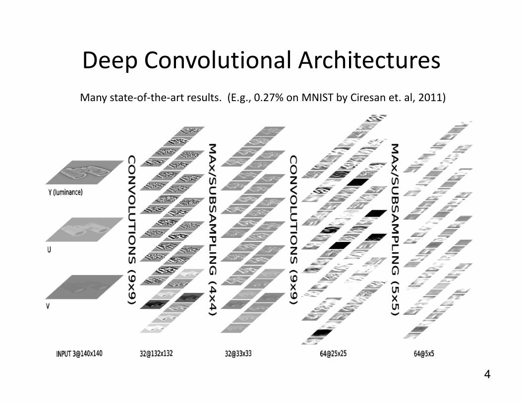
Deep Convolutional Architectures

Many state-of-the-art results. (E.g., 0.27% on MNIST by Ciresan et. al, 2011)

4

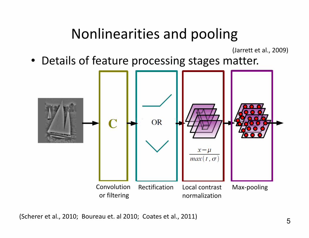
Nonlinearities and pooling

• Details of feature processing stages matter.(Jarrett et al., 2009)

5

Local contrast

normalization

Max-poolingRectificationConvolution

or filtering

(Scherer et al., 2010; Boureau et. al 2010; Coates et al., 2011)

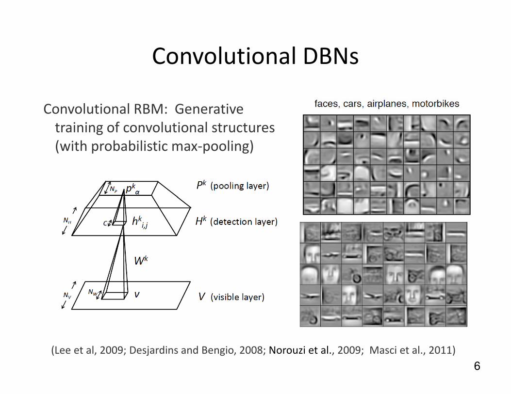
Convolutional DBNs

Convolutional RBM: Generative

training of convolutional structures

(with probabilistic max-pooling)

6

(Lee et al, 2009; Desjardins and Bengio, 2008; Norouzi et al., 2009; Masci et al., 2011)

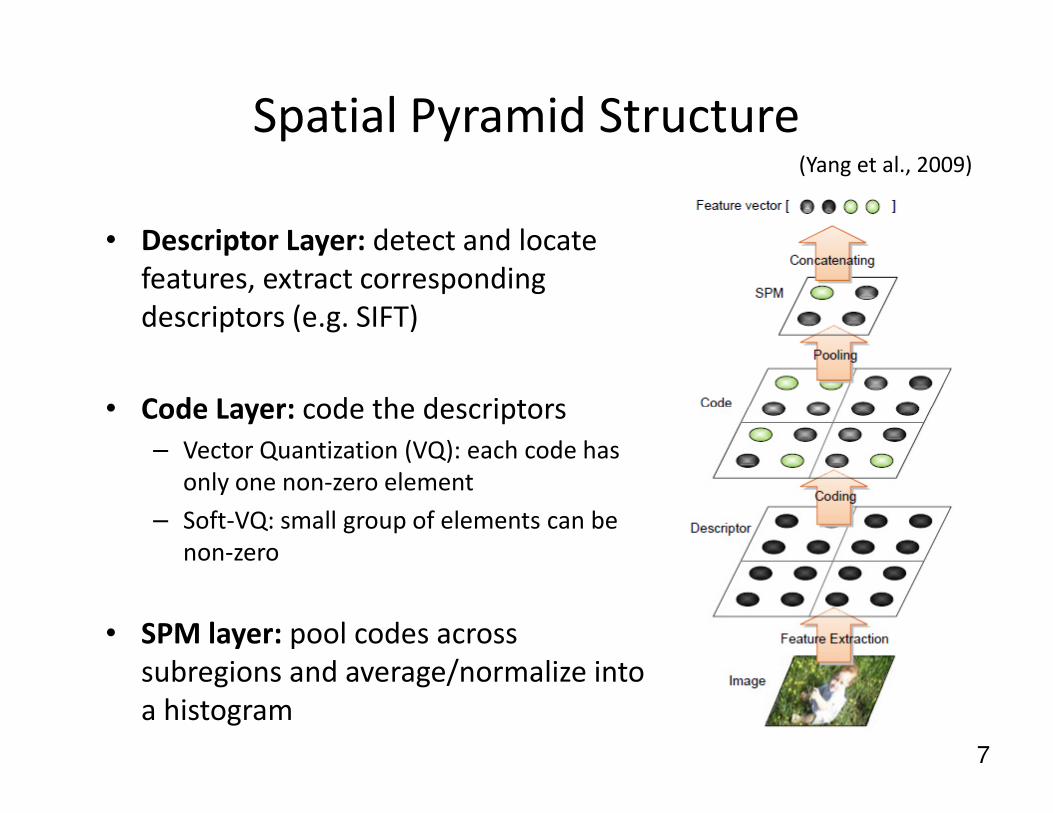
Spatial Pyramid Structure

• Descriptor Layer: detect and locate

features, extract corresponding

descriptors (e.g. SIFT)

• Code Layer: code the descriptors

(Yang et al., 2009)

7

• Code Layer: code the descriptors

– Vector Quantization (VQ): each code has

only one non-zero element

– Soft-VQ: small group of elements can be

non-zero

• SPM layer: pool codes across

subregions and average/normalize into

a histogram

Improving the coding step

• Modify the Coding step to produce

better feature representations

– Sparse coding

• Sparse like VQ

• Multiple non-zeros (more expressive)

– Local Coordinate coding

(Yang et al., 2009)

8

– Local Coordinate coding

Experimental results

• Competitive performance to other state-of-

the-art methods using a single type of

features on object recognition benchmarks

• E.g.: Caltech 101 (30 examples per class)

– Using pixel representation: ~65% accuracy (Jarret

9

– Using pixel representation: ~65% accuracy (Jarret

et al., 2009; Lee et al., 2009; and many others)

– Using SIFT representation: 73~77% accuracy (Yang

et al., 2009; Jarret et al., 2009, Boureau et al.,

2011, and many others)

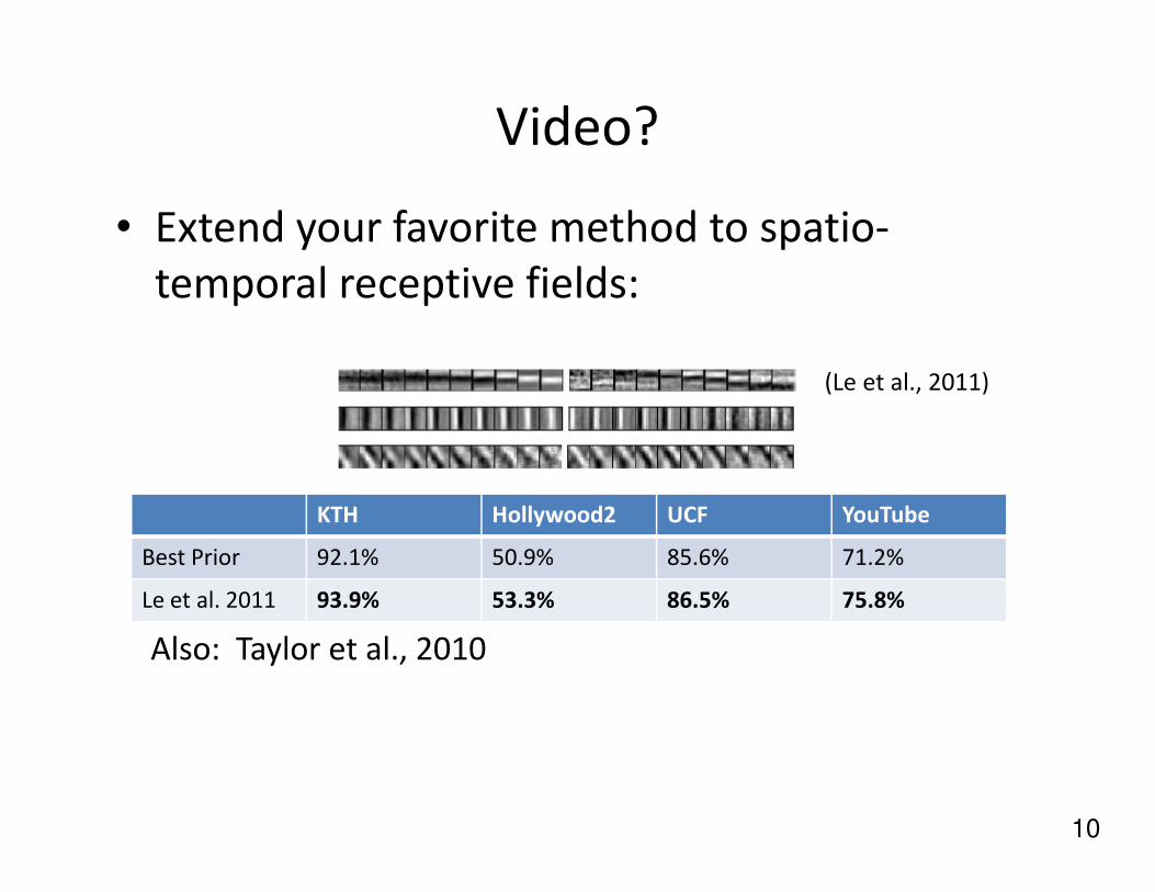
Video?

• Extend your favorite method to spatio-

temporal receptive fields:

(Le et al., 2011)

10

KTH Hollywood2 UCF YouTube

Best Prior 92.1% 50.9% 85.6% 71.2%

Le et al. 2011 93.9% 53.3% 86.5% 75.8%

Also: Taylor et al., 2010

Outline

• Deep learning

– Greedy layer-wise training (for supervised learning)

– Deep belief nets

– Stacked denoising auto-encoders

– Stacked predictive sparse coding

11

– Stacked predictive sparse coding

– Deep Boltzmann machines

• Applications

– Vision

– Audio

– Language

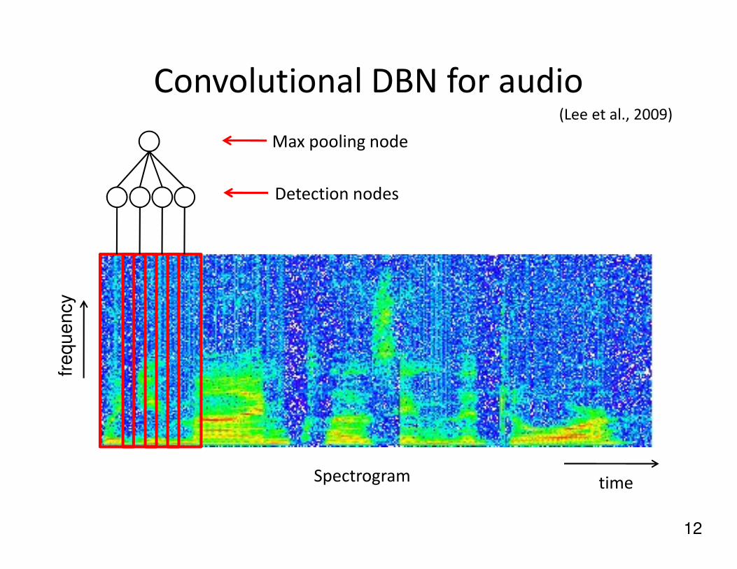
Convolutional DBN for audio

Detection nodes

Max pooling node

(Lee et al., 2009)

12

Spectrogram time

fre

qu

en

cy

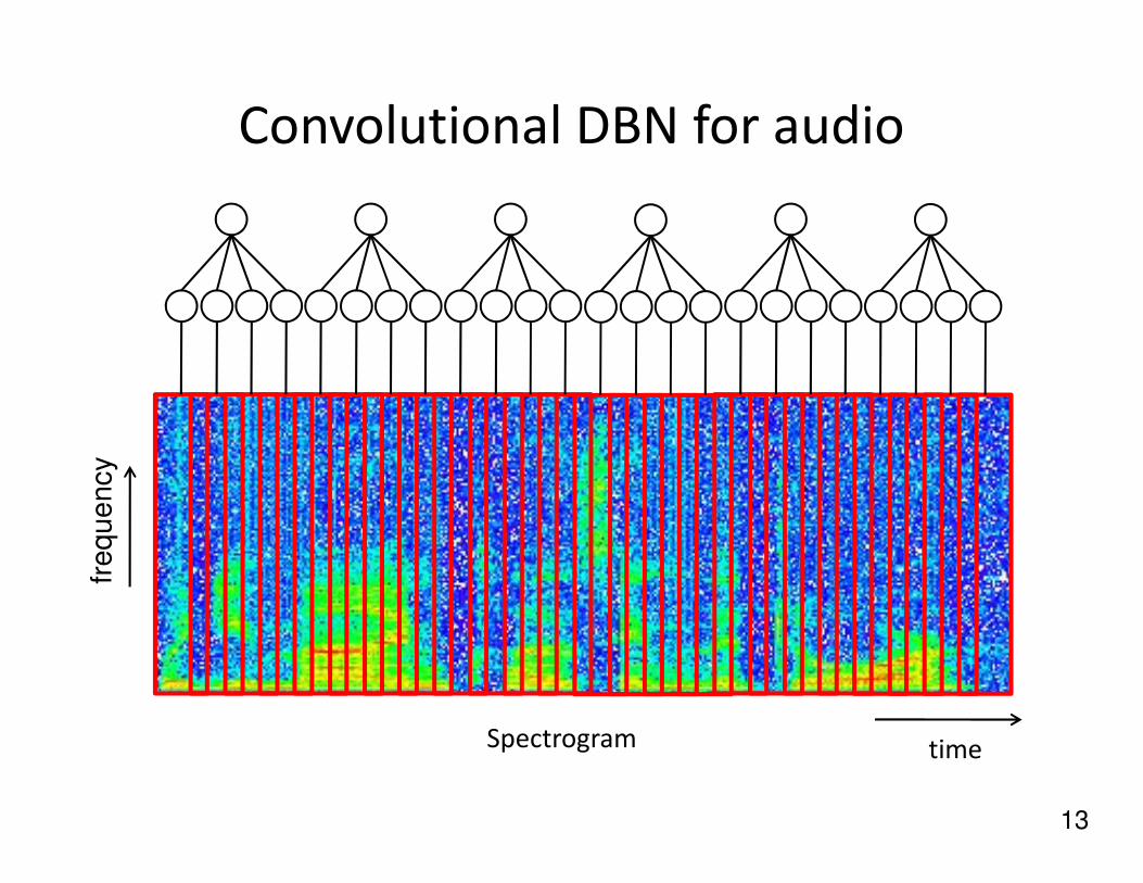
Convolutional DBN for audio

13

Spectrogram time

fre

qu

en

cy

CDBNs for speech

Trained on unlabeled TIMIT corpus

14

Learned first-layer bases

Experimental Results

• Speaker identification

• Phone classification

TIMIT Speaker identification Accuracy

Prior art (Reynolds, 1995) 99.7%

Convolutional DBN 100.0%

(Lee et al., 2009)

15

• Phone classificationTIMIT Phone classification Accuracy

Clarkson et al. (1999) 77.6%

Gunawardana et al. (2005) 78.3%

Sung et al. (2007) 78.5%

Petrov et al. (2007) 78.6%

Sha & Saul (2006) 78.9%

Yu et al. (2009) 79.2%

Convolutional DBN 80.3%

Phone recognition using DBNs

• Pre-training RBMs followed by fine-tuning

with back propagation

(Dahl et al., 2010; Mohamed et al., 2011)

16

Phone recognition using DBNs

• Can use predicted labels to recognize phones

in stream of audio with HMM.

(Dahl et al., 2010; Mohamed et al., 2011)

17

+1

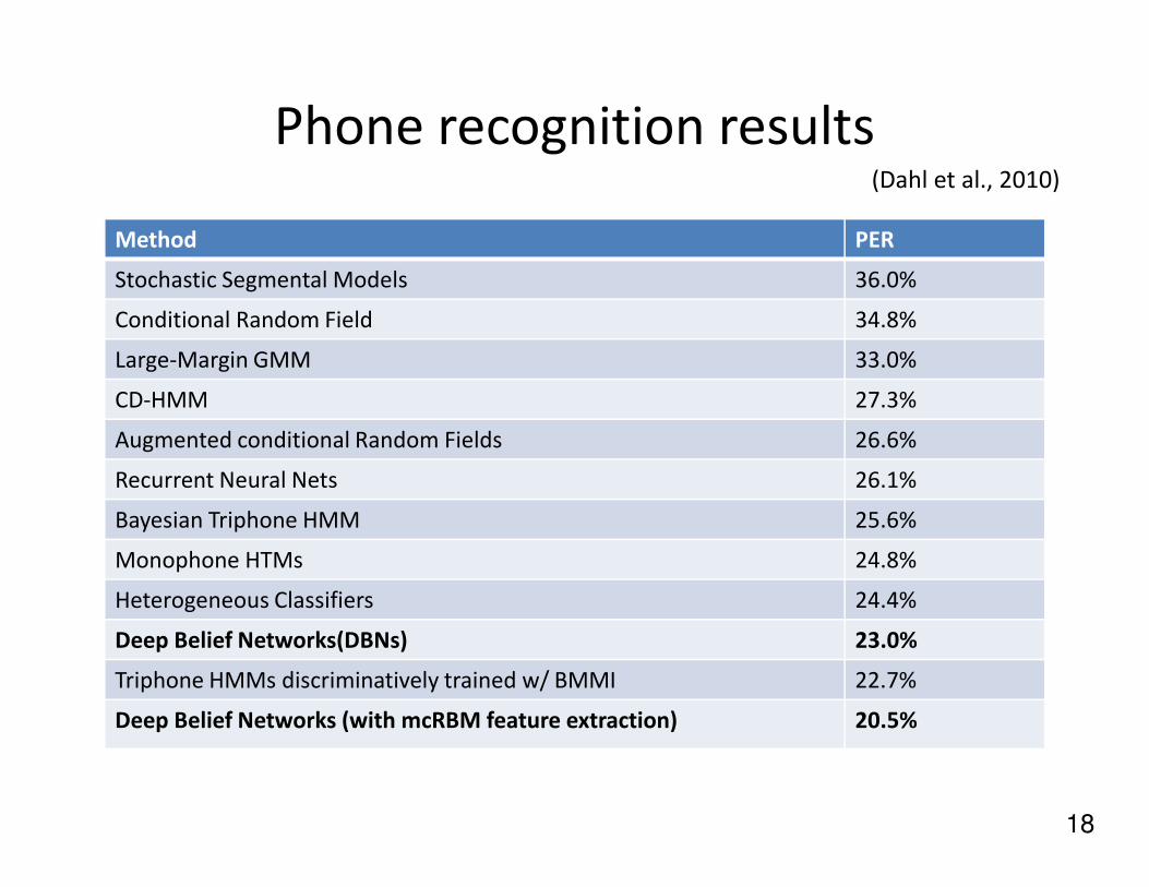
Phone recognition results

Method PER

Stochastic Segmental Models 36.0%

Conditional Random Field 34.8%

Large-Margin GMM 33.0%

CD-HMM 27.3%

Augmented conditional Random Fields 26.6%

(Dahl et al., 2010)

18

Augmented conditional Random Fields 26.6%

Recurrent Neural Nets 26.1%

Bayesian Triphone HMM 25.6%

Monophone HTMs 24.8%

Heterogeneous Classifiers 24.4%

Deep Belief Networks(DBNs) 23.0%

Triphone HMMs discriminatively trained w/ BMMI 22.7%

Deep Belief Networks (with mcRBM feature extraction) 20.5%

Outline

• Deep learning

– Greedy layer-wise training (for supervised learning)

– Deep belief nets

– Stacked denoising auto-encoders

– Stacked predictive sparse coding

19

– Stacked predictive sparse coding

– Deep Boltzmann machines

• Applications

– Vision

– Audio

– Language

Language modeling

• Language Models

– Estimating the probability of the next word w given a sequence of words

• Baseline approach in NLP

– N-gram models (with smoothing):

20

– N-gram models (with smoothing):

• Deep Learning approach

– Bengio et al. (2000, 2003): via Neural network

– Mnih and Hinton (2007): via RBMs

Predicting the next wordBengio et al. (2000, 2003)

Neural Net

Predict:

21

w1 w2 w3

… 0 1 0 0 0 0 … … 0 0 0 1 0 0 … … 1 0 0 0 0 0 …

0.2 1.6 0.9 1.20.1 0.4 -1.3 0.20.9 -0.2 0.8 0.2

C C C

Shared

Weights

A unified architecture for NLP

• Main idea: use as unified architecture for NLP

– Deep Neural Network

– Trained jointly with different tasks (feature sharing

and multi-task learning)

(Collobert and Weston, 2009)

22

and multi-task learning)

• Shows the generality of the architecture

General Deep Architecture for NLP

Basic features (e.g., word,

capitalization, relative position)

Embedding by lookup table

(Collobert and Weston, 2009)

23

Convolution (higher-level features

that fold in context)

Max pooling

Supervised learning

Other NLP tasks

• Part-Of-Speech Tagging (POS)– mark up the words in a text (corpus) as corresponding

to a particular tag• E.g. Noun, adverb, ...

• Chunking– Also called shallow parsing

(Collobert and Weston, 2009)

24

– Also called shallow parsing

– In the view of phrase: Labeling phrase to syntactic constituents

• E.g. NP (noun phrase), VP (verb phrase), …

– In the view of word: Labeling word to syntactic role in a phrase

• E.g. B-NP (beginning of NP), I-VP (inside VP), …

Other NLP tasks

• Named Entity Recognition (NER)

– In the view of thought group: Given a stream of

text, determine which items in the text map to

proper names

– E.g., labeling “atomic elements” into “PERSON”,

(Collobert and Weston, 2009)

25

– E.g., labeling “atomic elements” into “PERSON”,

“COMPANY”, “LOCATION”

• Semantic Role Labeling (SRL)

– In the view of sentence: giving a semantic role to a

syntactic constituent of a sentence

– E.g. [John]ARG0 [ate]REL [the apple]ARG1 (Proposition Bank)

• An Annotated Corpus of Semantic Roles (Palmer et al.)

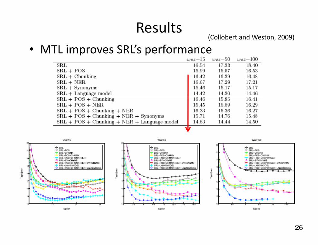
Results

• MTL improves SRL’s performance(Collobert and Weston, 2009)

26

Summary

• Training deep architectures

– Unsupervised pre-training helps training deep networks

– Deep belief nets, Stacked denoising auto-encoders, Stacked predictive sparse coding, Deep Boltzmann machines

27

Boltzmann machines

• Deep learning algorithms and unsupervised feature learning algorithms show promising results in many applications

– vision, audio, natural language processing, etc.