workshop on traffic assignment with equilibrium methods · workshop on traffic assignment with...
TRANSCRIPT
Workshop on Traffic Workshop on Traffic Assignment with Equilibrium Assignment with Equilibrium
MethodsMethods
Presented by:Presented by:David Boyce and Michael FlorianDavid Boyce and Michael Florian
Northwestern University and University of MontrealNorthwestern University and University of Montreal
Sponsored by:Sponsored by:Subcommittee on Network Equilibrium Modeling Subcommittee on Network Equilibrium Modeling
Transportation Network Modeling CommitteeTransportation Network Modeling Committee
January 9, 2005, 8:30 am January 9, 2005, 8:30 am –– 12:00 pm12:00 pm
Contents of second partContents of second part
►►Variable demand equilibrium assignmentVariable demand equilibrium assignment
►►MultiMulti--modal models : equilibrationmodal models : equilibration
►►Some large scale applicationsSome large scale applications
►►Stochastic user equilibrium assignmentStochastic user equilibrium assignment
Variable demand equilibrium Variable demand equilibrium assignment assignment
►► The demand for travel is assumed to be The demand for travel is assumed to be given by a direct demand function which given by a direct demand function which has the property that as travel time (cost) has the property that as travel time (cost) increases the demand decreasesincreases the demand decreases
►►The network equilibrium is established when The network equilibrium is established when all used routes are of equal time (cost) and all used routes are of equal time (cost) and the travel time leads to a demand which the travel time leads to a demand which yields the equilibrium link flowsyields the equilibrium link flows
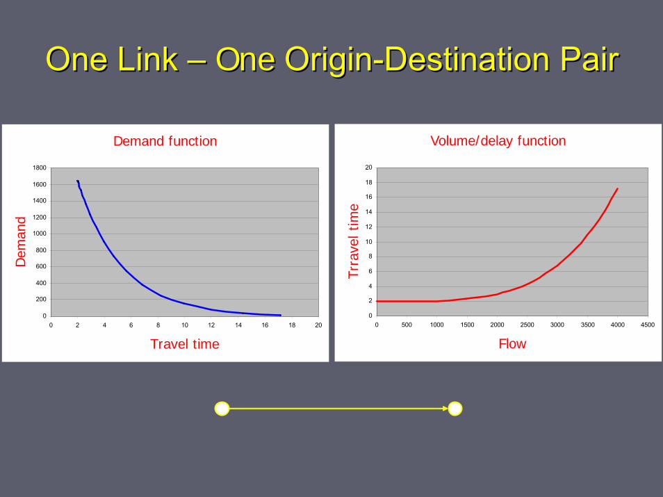
One Link One Link –– OneOne OriginOrigin--Destination PairDestination Pair
Volume/delay function
0
2
4
6
8
10
12
14
16
18
20
0 500 1000 1500 2000 2500 3000 3500 4000 4500
FlowTr
rave
l tim
e
Demand function
0
200
400
600
800
1000
1200
1400
1600
1800
0 2 4 6 8 10 12 14 16 18 20
Travel time
Dem
and
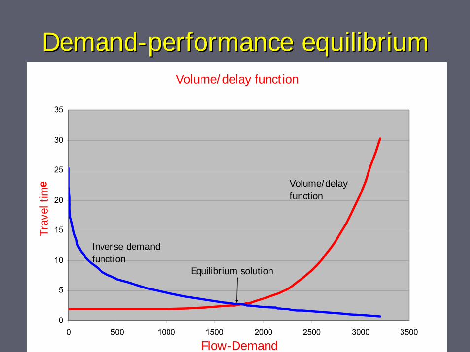
DemandDemand--performance equilibriumperformance equilibriumVolume/delay function
0
5
10
15
20
25
30
35
0 500 1000 1500 2000 2500 3000 3500
Flow-Demand
Trav
el t
ime
Inverse demand function
Volume/delay function
Equilibrium solution
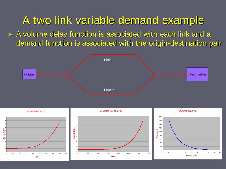
A two link variable demand exampleA two link variable demand example►► A volume delay function is associated with each link and a A volume delay function is associated with each link and a
demand function is associated with the origindemand function is associated with the origin--destination pairdestination pair
Origin Destination
Volume/delay function
0
2
4
6
8
10
12
14
16
18
20
0 500 1000 1500 2000 2500 3000 3500 4000 4500
Flow
Trra
vel t
ime
Demand function
0
200
400
600
800
1000
1200
1400
1600
1800
0 2 4 6 8 10 12 14 16 18 20
Travel timeD
eman
d
Link 1
Link 2
Volume/delay function
0
5
10
15
20
25
30
35
0 500 1000 1500 2000 2500 3000 3500
Flow
Trra
vel t
ime
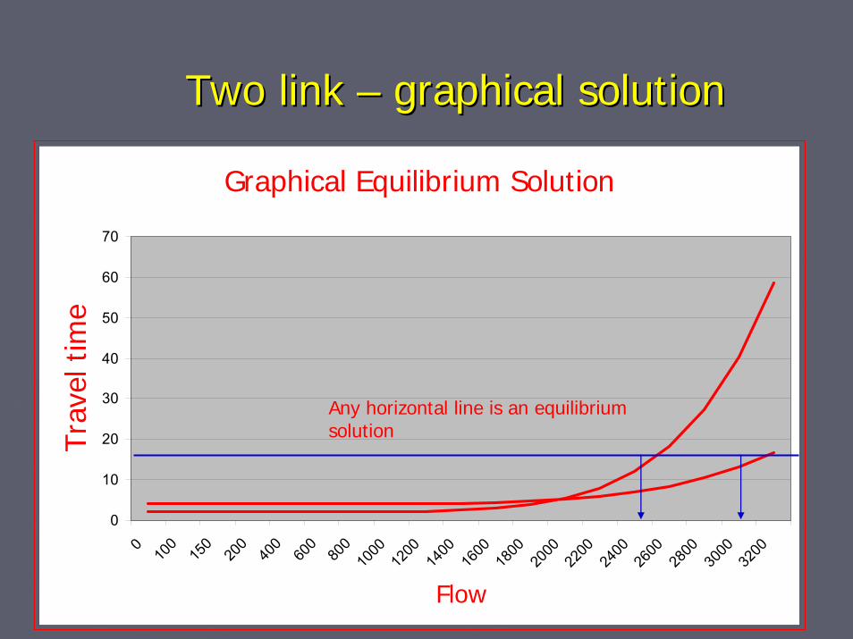
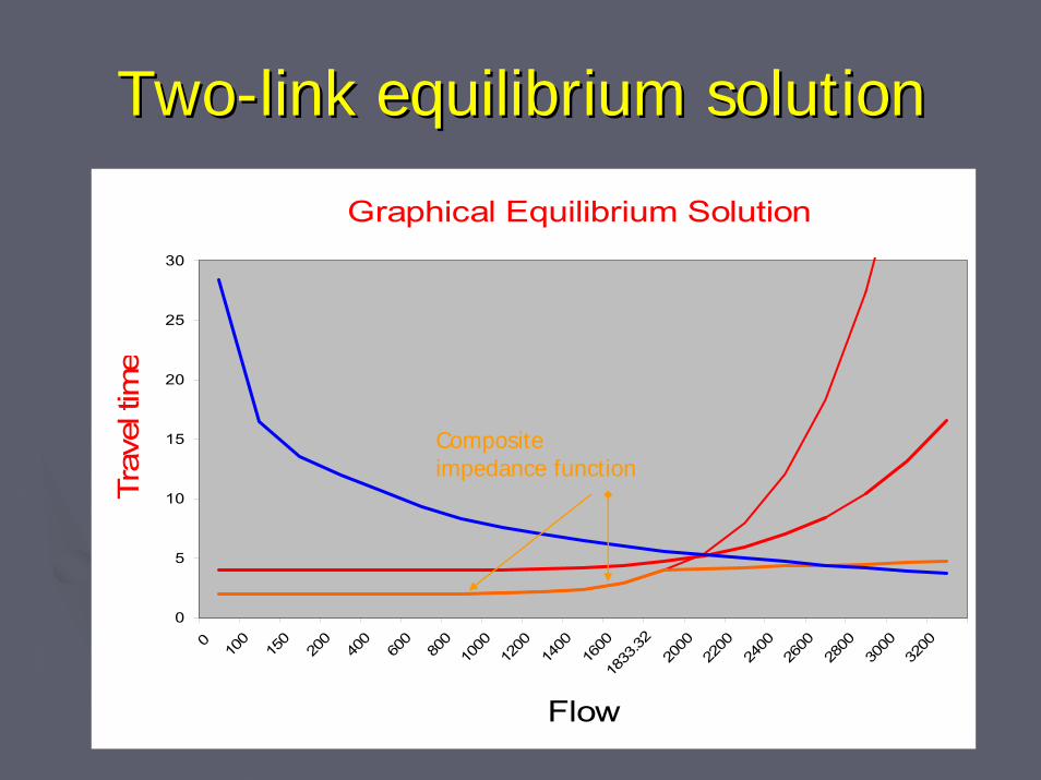
Two link Two link –– graphical solutiongraphical solution
Graphical Equilibrium Solution
0
10
20
30
40
50
60
70
010
015
020
040
060
080
010
0012
0014
0016
0018
0020
0022
0024
0026
0028
0030
0032
00
Flow
Trav
el t
ime
Any horizontal line is an equilibrium solution
The twoThe two--link equilibrium solutionlink equilibrium solution
►► The travel time on both links is the sameThe travel time on both links is the same►► The demand on each link is that which corresponds to the The demand on each link is that which corresponds to the
travel time of the two pathstravel time of the two paths►► One computes the aggregate of the two volume/delay One computes the aggregate of the two volume/delay
functions. It is the lower free flow time volume/delay functions. It is the lower free flow time volume/delay function until it reaches the free flow time of the higher function until it reaches the free flow time of the higher travel time function. Then for each equilibrium travel timetravel time function. Then for each equilibrium travel time
►► One adds the corresponding flow on the two links.One adds the corresponding flow on the two links.►► Then the intersection of the inverse demand function with Then the intersection of the inverse demand function with
the aggregate impedance curve is the equilibrium solution the aggregate impedance curve is the equilibrium solution for the link that gives the minimum travel timefor the link that gives the minimum travel time
TwoTwo--link equilibrium solutionlink equilibrium solution
Equilibrium solution
O-D impedance function
Graphical Equilibrium Solution
0
5
10
15
20
25
30
0
100
150
200
400
600
800
1000
1200
1400
1600
1833
.3220
0022
0024
0026
0028
0030
0032
00
Flow
Trav
el ti
me
Composite impedance function
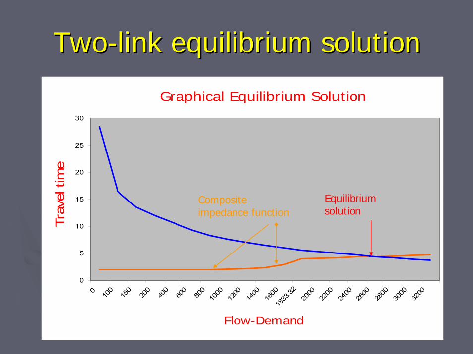
TwoTwo--link equilibrium solutionlink equilibrium solution
Equilibrium solution
O-D impedance function
Graphical Equilibrium Solution
0
5
10
15
20
25
30
0
100
150
200
400
600
800
1000
1200
1400
1600
1833
.3220
0022
0024
0026
0028
0030
0032
00
Flow-Demand
Trav
el tim
e
Composite impedance function
Equilibrium solution
Variable demand network equilibriumVariable demand network equilibrium
►►This is a well solved problemThis is a well solved problem►►Numerous algorithms have been proposed Numerous algorithms have been proposed
to solve this problemto solve this problem►►The applications are few since the demand The applications are few since the demand
is usually not specified by a direct demand is usually not specified by a direct demand functionfunction
►►Has been used for combined mode choice Has been used for combined mode choice assignment equilibrationassignment equilibration
►►Variable demand equilibrium assignmentVariable demand equilibrium assignment
►►MultiMulti--modal models : equilibrationmodal models : equilibration
►►Some large scale applicationsSome large scale applications
►►Stochastic user equilibrium assignmentStochastic user equilibrium assignment
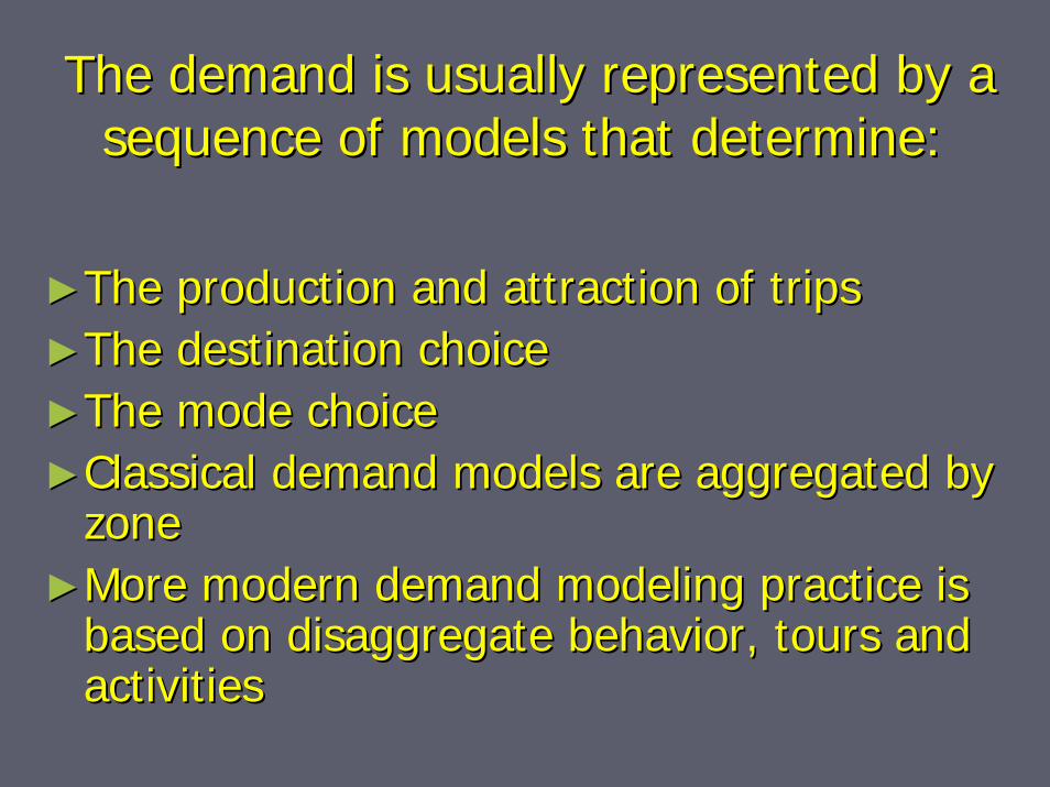
The demand is usually represented by a The demand is usually represented by a sequence of models that determinesequence of models that determine::
►►The production and attraction of tripsThe production and attraction of trips►►The destination choiceThe destination choice►►The mode choiceThe mode choice►►Classical demand models are aggregated by Classical demand models are aggregated by
zonezone►►More modern demand modeling practice is More modern demand modeling practice is
based on disaggregate behavior, tours and based on disaggregate behavior, tours and activitiesactivities
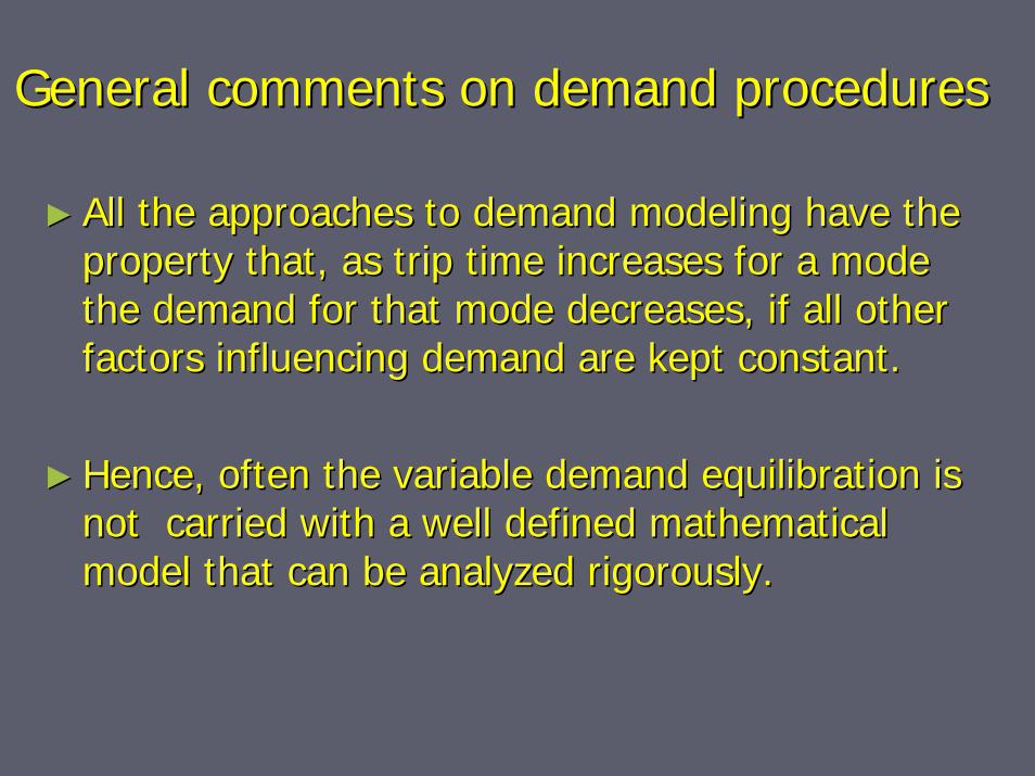
General comments on demand proceduresGeneral comments on demand procedures
►► All the approaches to demand modeling have the All the approaches to demand modeling have the property that, as trip time increases for a mode property that, as trip time increases for a mode the demand for that mode decreases, if all other the demand for that mode decreases, if all other factors influencing demand are kept constant.factors influencing demand are kept constant.
►► Hence, often the variable demand equilibration is Hence, often the variable demand equilibration is not carried with a well defined mathematical not carried with a well defined mathematical model that can be analyzed rigorously.model that can be analyzed rigorously.
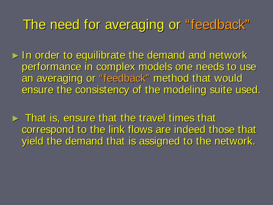
The need for averaging or The need for averaging or ““feedbackfeedback””
►► In order to equilibrate the demand and network In order to equilibrate the demand and network performance in complex models one needs to use performance in complex models one needs to use an averaging or an averaging or ““feedbackfeedback”” method that would method that would ensure the consistency of the modeling suite used.ensure the consistency of the modeling suite used.
►► That is, ensure that the travel times that That is, ensure that the travel times that correspond to the link flows are indeed those that correspond to the link flows are indeed those that yield the demand that is assigned to the network.yield the demand that is assigned to the network.
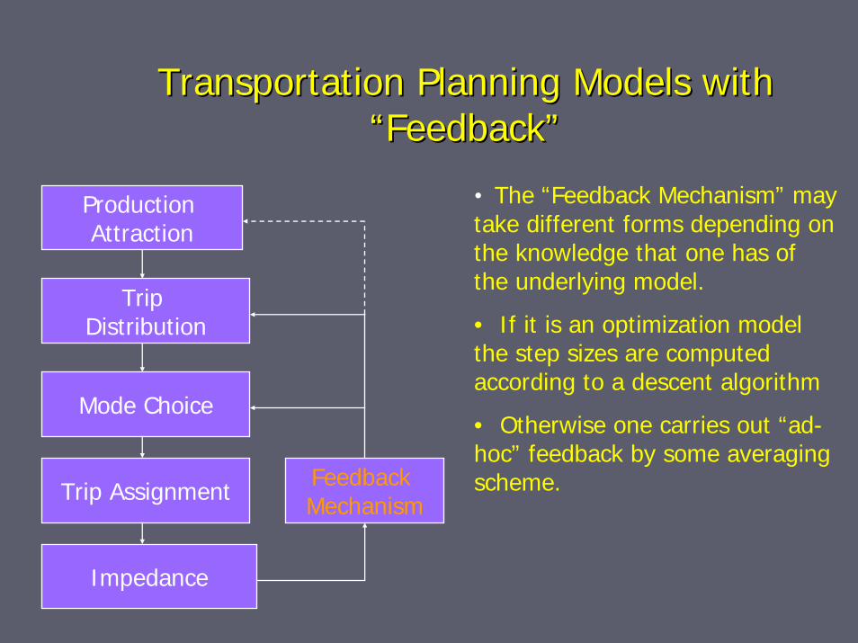
Transportation Planning Models with Transportation Planning Models with ““FeedbackFeedback””
Production Attraction
Trip Distribution
Mode Choice
Trip Assignment
Impedance
Feedback Mechanism
• The “Feedback Mechanism” may take different forms depending on the knowledge that one has of the underlying model.
• If it is an optimization model the step sizes are computed according to a descent algorithm
• Otherwise one carries out “ad-hoc” feedback by some averaging scheme.
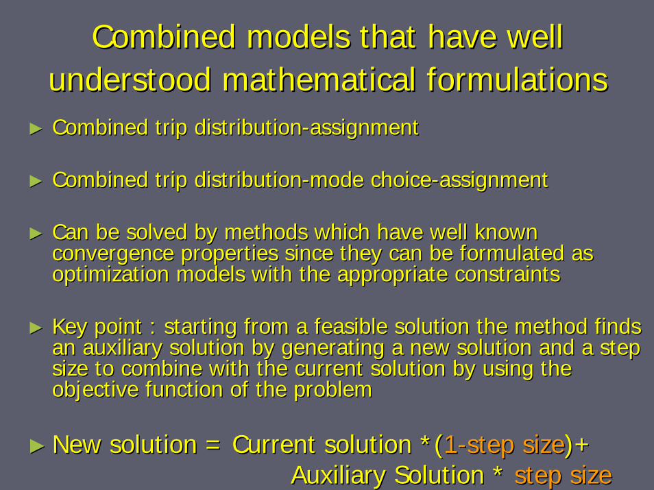
Combined models that have well Combined models that have well understood mathematical formulationsunderstood mathematical formulations
►► Combined trip distributionCombined trip distribution--assignmentassignment
►► Combined trip distributionCombined trip distribution--mode choicemode choice--assignmentassignment
►► Can be solved by methods which have well known Can be solved by methods which have well known convergence properties since they can be formulated as convergence properties since they can be formulated as optimization models with the appropriate constraintsoptimization models with the appropriate constraints
►► Key point : starting from a feasible solution the method finds Key point : starting from a feasible solution the method finds an auxiliary solution by generating a new solution and a step an auxiliary solution by generating a new solution and a step size to combine with the current solution by using the size to combine with the current solution by using the objective function of the problemobjective function of the problem
►► New solution = Current solution *(New solution = Current solution *(11--step sizestep size)+)+Auxiliary Solution * Auxiliary Solution * step sizestep size
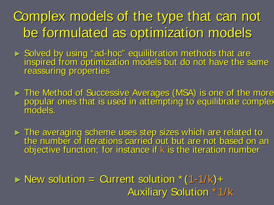
Complex models of the type that can not Complex models of the type that can not be formulated as optimization modelsbe formulated as optimization models
►► Solved by using Solved by using ““adad--hochoc”” equilibration methods that are equilibration methods that are inspired from optimization models but do not have the same inspired from optimization models but do not have the same reassuring propertiesreassuring properties
►► The Method of Successive Averages (MSA) is one of the more The Method of Successive Averages (MSA) is one of the more popular ones that is used in attempting to equilibrate complexpopular ones that is used in attempting to equilibrate complexmodels.models.
►► The averaging scheme uses step sizes which are related to The averaging scheme uses step sizes which are related to the number of iterations carried out but are not based on an the number of iterations carried out but are not based on an objective function; for instance if objective function; for instance if kk is the iteration numberis the iteration number
►► New solution = Current solution *(New solution = Current solution *(11--1/k1/k)+)+Auxiliary SolutionAuxiliary Solution *1/k*1/k
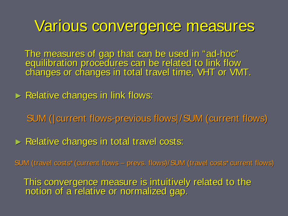
Various convergence measuresVarious convergence measures
The measures of gap that can be used in The measures of gap that can be used in ““adad--hochoc””equilibration procedures can be related to link flow equilibration procedures can be related to link flow changes or changes in total travel time, VHT or VMT.changes or changes in total travel time, VHT or VMT.
►► Relative changes in link flows:Relative changes in link flows:
SUM (|current flowsSUM (|current flows--previous flows|/SUM (current flows)previous flows|/SUM (current flows)
►► Relative changes in total travel costs:Relative changes in total travel costs:
SUM (travel costs*(current flows SUM (travel costs*(current flows –– prevs. flows)/SUM (travel costs*current flows)prevs. flows)/SUM (travel costs*current flows)
This convergence measure is intuitively related to the This convergence measure is intuitively related to the notion of a relative or normalized gap.notion of a relative or normalized gap.
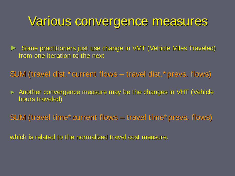
Various convergence measuresVarious convergence measures
►► Some practitioners just use change in VMT (Vehicle Miles TraveleSome practitioners just use change in VMT (Vehicle Miles Traveled) d) from one iteration to the nextfrom one iteration to the next
SUM (travel dist.*current flows SUM (travel dist.*current flows –– travel dist.*travel dist.*prevsprevs. flows). flows)
►► Another convergence measure may be the changes in VHT (Vehicle Another convergence measure may be the changes in VHT (Vehicle hours traveled)hours traveled)
SUM (travel time*current flows SUM (travel time*current flows –– travel time*prevs. flows)travel time*prevs. flows)
which is related to the normalized travel cost measure.which is related to the normalized travel cost measure.
Various convergence measuresVarious convergence measures
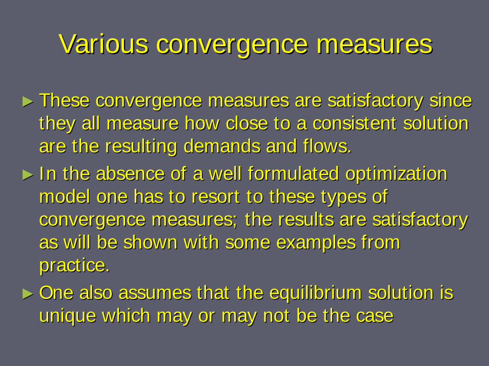
►► These convergence measures are satisfactory since These convergence measures are satisfactory since they all measure how close to a consistent solution they all measure how close to a consistent solution are the resulting demands and flows. are the resulting demands and flows.
►► In the absence of a well formulated optimization In the absence of a well formulated optimization model one has to resort to these types of model one has to resort to these types of convergence measures; the results are satisfactory convergence measures; the results are satisfactory as will be shown with some examples from as will be shown with some examples from practice.practice.
►► One also assumes that the equilibrium solution is One also assumes that the equilibrium solution is unique which may or may not be the caseunique which may or may not be the case
►►Variable demand equilibrium assignmentVariable demand equilibrium assignment
►►MultiMulti--modal models : equilibrationmodal models : equilibration
►►Some large scale applicationsSome large scale applications
►►Stochastic user equilibrium assignmentStochastic user equilibrium assignment
Examples of Equilibration:Examples of Equilibration:Some examples derived from practiceSome examples derived from practice
where where ““feedbackfeedback”” was usedwas used
Metro Portland, ORWinnipeg, Manitoba
Santiago, ChileSCAG, California
(None of these are current models)
The Metro Portland Model Study on The Metro Portland Model Study on EquilibrationEquilibration
►► This part of the presentation is based on work This part of the presentation is based on work done by Dick Walker, Cindy Pederson and Scott done by Dick Walker, Cindy Pederson and Scott HigginsHiggins
►► The paper is entitled The paper is entitled ““ Equilibrating the Input and Equilibrating the Input and Output Impedances in the Demand Modeling Output Impedances in the Demand Modeling ProcessProcess”” November 1995 November 1995
►► The paper is publicly availableThe paper is publicly available
The Metro Portland Model Study on The Metro Portland Model Study on EquilibrationEquilibration
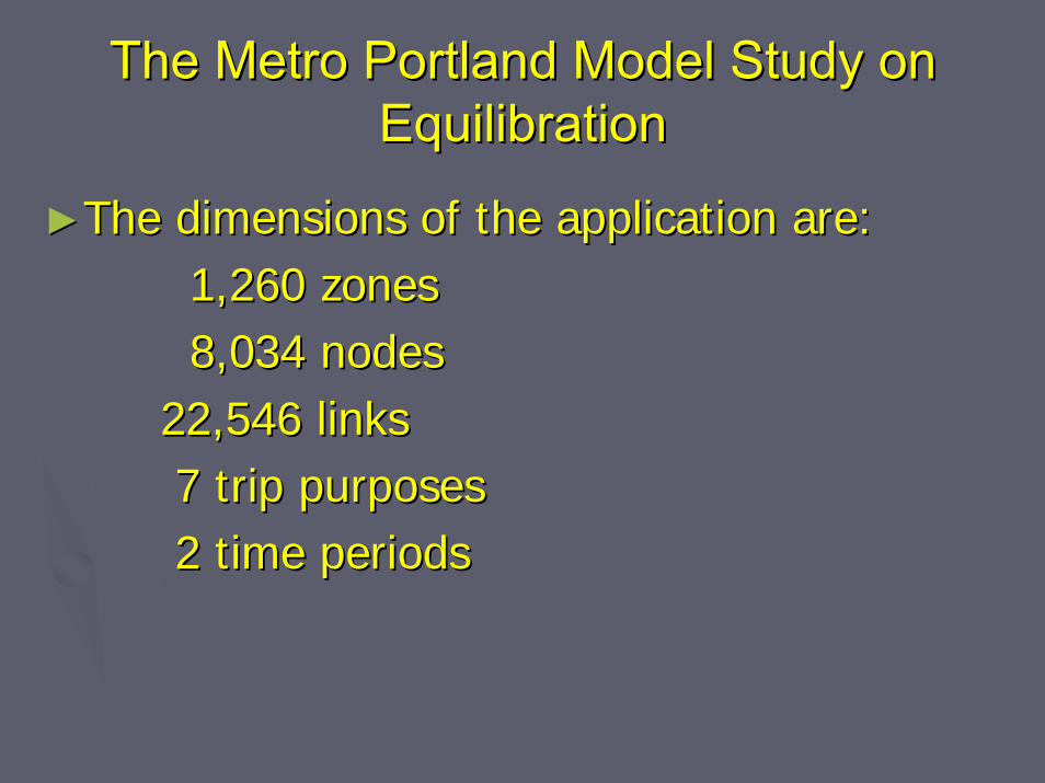
►►The dimensions of the application are:The dimensions of the application are:1,260 zones1,260 zones8,034 nodes8,034 nodes
22,546 links22,546 links7 trip purposes7 trip purposes2 time periods2 time periods
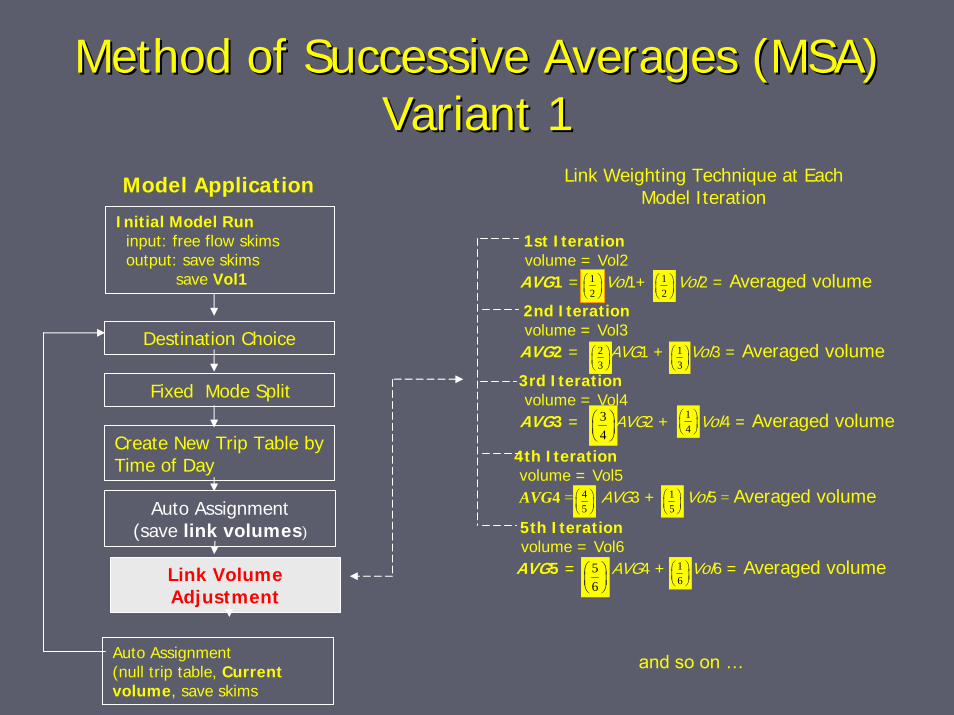
Method of Successive Averages (MSA) Method of Successive Averages (MSA) Variant 1Variant 1
Link Weighting Technique at Each Model IterationModel Application
Initial Model Runinput: free flow skimsoutput: save skims
save Vol1
1st Iterationvolume = Vol2
AVG1 = Vol1+ Vol2 = Averaged volume
2nd Iterationvolume = Vol3
AVG2 = AVG1 + Vol3 = Averaged volume
12
⎛ ⎞⎜ ⎟⎝ ⎠
12
⎛ ⎞⎜ ⎟⎝ ⎠
13
⎛ ⎞⎜ ⎟⎝ ⎠
3rd Iterationvolume = Vol4
AVG3 = AVG2 + Vol4 = Averaged volume
23
⎛ ⎞⎜ ⎟⎝ ⎠
34
⎛ ⎞⎜ ⎟⎝ ⎠
14
⎛ ⎞⎜ ⎟⎝ ⎠
4th Iterationvolume = Vol5AVG4 = AVG3 + Vol5 = Averaged volume4
5⎛ ⎞⎜ ⎟⎝ ⎠
15
⎛ ⎞⎜ ⎟⎝ ⎠
5th Iterationvolume = Vol6
AVG5 = AVG4 + Vol6 = Averaged volume56
⎛ ⎞⎜ ⎟⎝ ⎠
16
⎛ ⎞⎜ ⎟⎝ ⎠
Destination Choice
Fixed Mode Split
Create New Trip Table by Time of Day
Auto Assignment(save link volumes)
Link VolumeAdjustment
Auto Assignment(null trip table, Current volume, save skims
and so on …
The implied step sizeThe implied step size
►►The step size used is in this variant of MSA The step size used is in this variant of MSA is simply 1/iteration numberis simply 1/iteration number
►►That is, the last volume obtained is given a That is, the last volume obtained is given a decreasing weight as the number of decreasing weight as the number of iterations increaseiterations increase
►► This is the most conventional form of the This is the most conventional form of the MSA methodMSA method
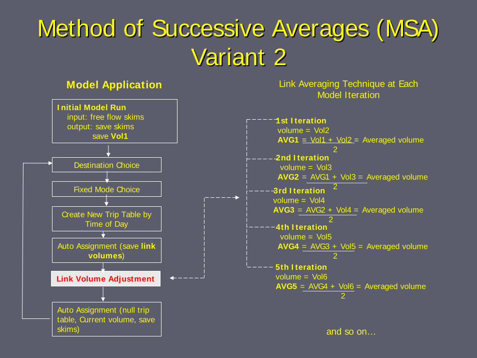
Method of Successive Averages (MSA) Method of Successive Averages (MSA) Variant 2Variant 2
Model Application Link Averaging Technique at Each Model Iteration
Initial Model Runinput: free flow skimsoutput: save skims
save Vol1
1st Iterationvolume = Vol2AVG1 = Vol1 + Vol2 = Averaged volume
22nd Iterationvolume = Vol3
AVG2 = AVG1 + Vol3 = Averaged volume23rd Iteration
volume = Vol4AVG3 = AVG2 + Vol4 = Averaged volume
24th Iterationvolume = Vol5
AVG4 = AVG3 + Vol5 = Averaged volume2
5th Iterationvolume = Vol6AVG5 = AVG4 + Vol6 = Averaged volume
2
Destination Choice
Fixed Mode Choice
Create New Trip Table by Time of Day
Auto Assignment (save link volumes)
Link Volume Adjustment
Auto Assignment (null trip table, Current volume, save skims) and so on…
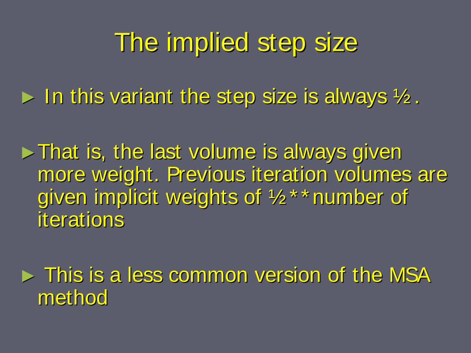
The implied step sizeThe implied step size
►► In this variant the step size is always In this variant the step size is always ½½..
►►That is, the last volume is always given That is, the last volume is always given more weight. Previous iteration volumes are more weight. Previous iteration volumes are given implicit weights of given implicit weights of ½½**number of **number of iterationsiterations
►► This is a less common version of the MSA This is a less common version of the MSA methodmethod
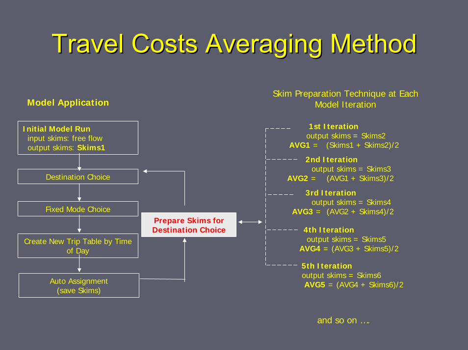
Travel Costs Averaging MethodTravel Costs Averaging Method
Skim Preparation Technique at Each Model IterationModel Application
Initial Model Runinput skims: free flowoutput skims: Skims1
Destination Choice
Fixed Mode Choice
Create New Trip Table by Time of Day
1st Iterationoutput skims = Skims2
AVG1 = (Skims1 + Skims2)/2
2nd Iterationoutput skims = Skims3
AVG2 = (AVG1 + Skims3)/2
3rd Iterationoutput skims = Skims4
AVG3 = (AVG2 + Skims4)/2
4th Iterationoutput skims = Skims5
AVG4 = (AVG3 + Skims5)/2
5th Iterationoutput skims = Skims6AVG5 = (AVG4 + Skims6)/2
Prepare Skims for Destination Choice
Auto Assignment(save Skims)
and so on ….
Impedance averagingImpedance averaging
►► This variant of MSA is less common but in some This variant of MSA is less common but in some circumstances it may be usefulcircumstances it may be useful
►► The results obtained resemble those obtained The results obtained resemble those obtained with link volume averaging but require more with link volume averaging but require more iterationsiterations
►► The next two slides show the convergence results The next two slides show the convergence results for VHT and VMT. Link flow differences were not for VHT and VMT. Link flow differences were not givengiven
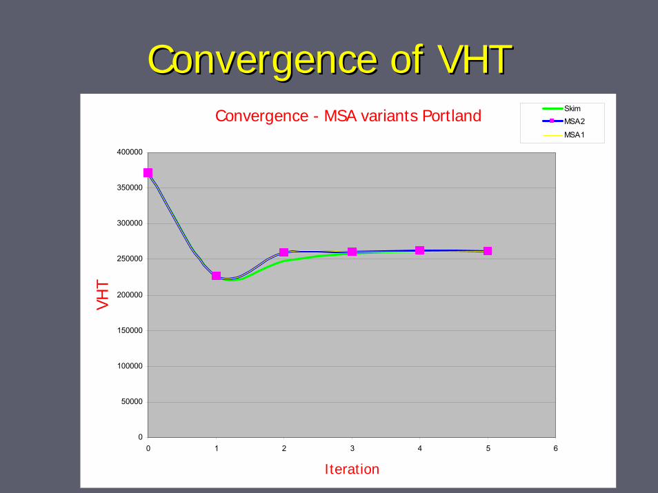
Convergence of VHTConvergence of VHTConvergence - MSA variants Portland
0
50000
100000
150000
200000
250000
300000
350000
400000
0 1 2 3 4 5 6
Iteration
VHT
SkimMSA2
MSA1
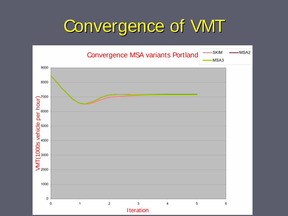
Convergence of VMTConvergence of VMTConvergence MSA variants Portland
0
1000
2000
3000
4000
5000
6000
7000
8000
9000
0 1 2 3 4 5 6
Iteration
VMT(
1000
s ve
hicl
e pe
r ho
ur)
SKIM MSA2
MSA3
The Winnipeg, Canada ModelThe Winnipeg, Canada Model
►► This application is based on a rather old data base. The This application is based on a rather old data base. The purpose here is to demonstrate the the equilibration purpose here is to demonstrate the the equilibration mechanism.mechanism.
►► The model is a rather conventional four step model where The model is a rather conventional four step model where the equilibration involves the trip distribution, the mode the equilibration involves the trip distribution, the mode choice and the assignment on both road and transit choice and the assignment on both road and transit networks.networks.
►► The problem size is modest: 154 zones, 1,100 nodes, 3000 The problem size is modest: 154 zones, 1,100 nodes, 3000 links, 67 transit lines, 2 modes, 1 trip purpose.links, 67 transit lines, 2 modes, 1 trip purpose.
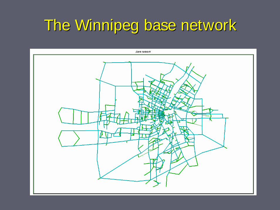
The Winnipeg base networkThe Winnipeg base network
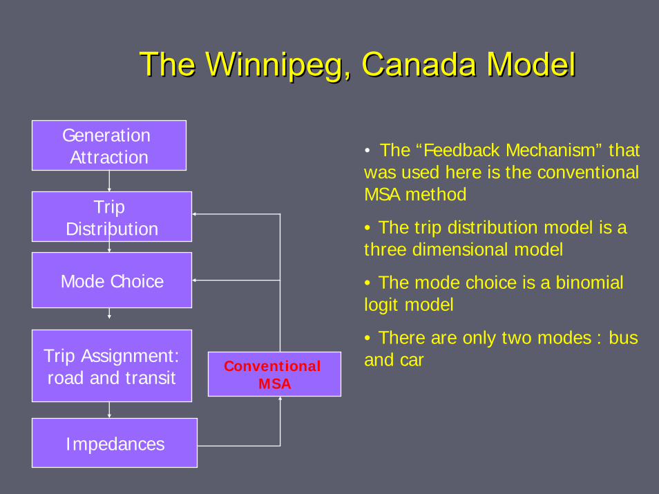
The Winnipeg, Canada ModelThe Winnipeg, Canada Model
Generation Attraction
Trip Distribution
Mode Choice
Trip Assignment:road and transit
Impedances
Conventional MSA
• The “Feedback Mechanism” that was used here is the conventional MSA method
• The trip distribution model is a three dimensional model
• The mode choice is a binomial logit model
• There are only two modes : bus and car
The Winnipeg, Canada ModelThe Winnipeg, Canada Model
►► The next two slides give the convergence The next two slides give the convergence results for the link difference and results for the link difference and normalized gap measures for two variants normalized gap measures for two variants of the trip distribution model: twoof the trip distribution model: two--dimensional and threedimensional and three--dimensional models.dimensional models.
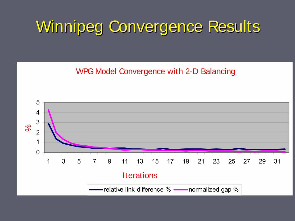
Winnipeg Convergence ResultsWinnipeg Convergence Results
WPG Model Convergence with 2-D Balancing
012345
1 3 5 7 9 11 13 15 17 19 21 23 25 27 29 31
%
relative link difference % normalized gap %
Iterations
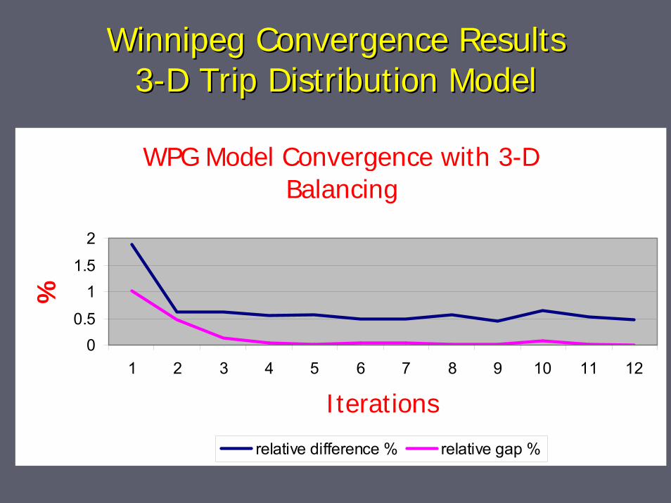
Winnipeg Convergence ResultsWinnipeg Convergence Results33--D Trip Distribution ModelD Trip Distribution Model
WPG Model Convergence with 3-D Balancing
00.5
11.5
2
1 2 3 4 5 6 7 8 9 10 11 12
Iterations
%
relative difference % relative gap %
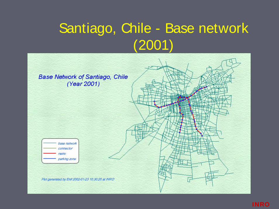
Santiago, Chile - Base network (2001)
INRO
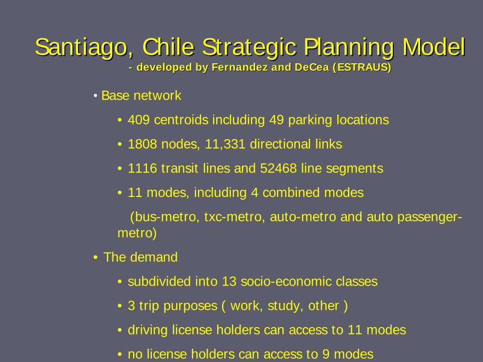
Santiago, Chile Strategic Planning ModelSantiago, Chile Strategic Planning Model-- developed by Fernandez and DeCea (ESTRAUS)developed by Fernandez and DeCea (ESTRAUS)
• Base network
• 409 centroids including 49 parking locations
• 1808 nodes, 11,331 directional links
• 1116 transit lines and 52468 line segments
• 11 modes, including 4 combined modes
(bus-metro, txc-metro, auto-metro and auto passenger-metro)
• The demand
• subdivided into 13 socio-economic classes
• 3 trip purposes ( work, study, other )
• driving license holders can access to 11 modes
• no license holders can access to 9 modes
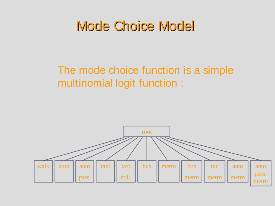
Mode Choice ModelMode Choice Model
The mode choice function is a simple multinomial logit function :
root
walk auto auto
pass.
taxi taxi
coll.
bus metro bus
metro
txc
metro
auto
metro
auto pass. metro
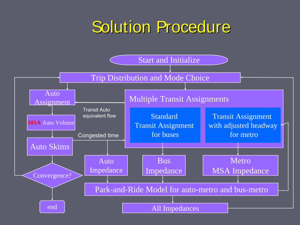
Solution ProcedureSolution Procedure
Multiple Transit Assignments
Standard Transit Assignment
for buses
Trip Distribution and Mode Choice
MetroMSA Impedance
AutoAssignment
Congested time
Transit Assignment with adjusted headway
for metro
BusImpedance
AutoImpedance
Park-and-Ride Model for auto-metro and bus-metro
Convergence?
end All Impedances
Start and Initialize
MSA Auto Volume
Transit Auto equivalent flow
Auto Skims
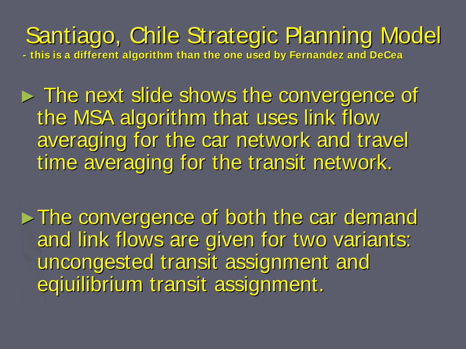
Santiago, Chile Strategic Planning ModelSantiago, Chile Strategic Planning Model-- this is a different algorithm than the one used by Fernandez anthis is a different algorithm than the one used by Fernandez and d DeCeaDeCea
►► The next slide shows the convergence of The next slide shows the convergence of the MSA algorithm that uses link flow the MSA algorithm that uses link flow averaging for the car network and travel averaging for the car network and travel time averaging for the transit network.time averaging for the transit network.
►►The convergence of both the car demand The convergence of both the car demand and link flows are given for two variants: and link flows are given for two variants: uncongesteduncongested transit assignment and transit assignment and eqiuilibriumeqiuilibrium transit assignment.transit assignment.
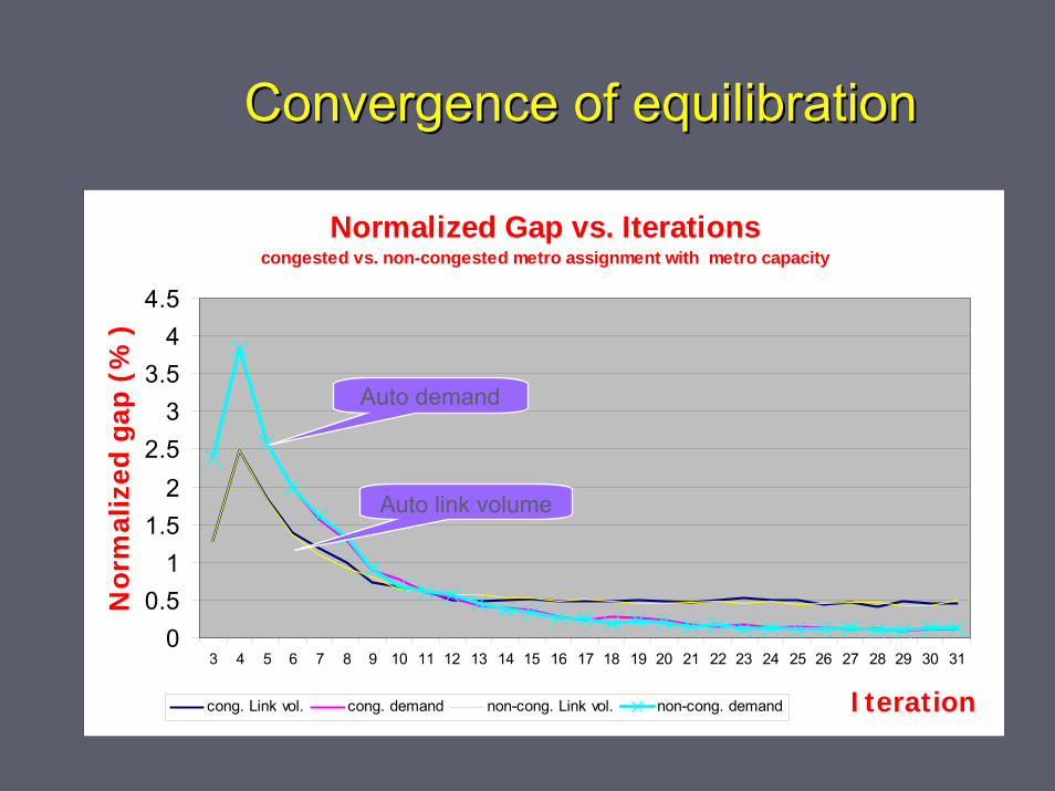
Convergence of equilibrationConvergence of equilibration
Normalized Gap vs. Iterationscongested vs. non-congested metro assignment with metro capacity
00.5
11.5
22.5
33.5
44.5
3 4 5 6 7 8 9 10 11 12 13 14 15 16 17 18 19 20 21 22 23 24 25 26 27 28 29 30 31
Iteration
Nor
mal
ized
gap
(%
)
cong. Link vol. cong. demand non-cong. Link vol. non-cong. demand
Auto demand
Auto link volume
The SCAG California ModelThe SCAG California Model
►► This is a very large model of the aggregate This is a very large model of the aggregate varietyvariety
►►The model dimensions are impressive:The model dimensions are impressive:15 modes15 modes4 time periods4 time periods13 trip purposes 13 trip purposes –– trip distribution modelstrip distribution models5 mode choice models5 mode choice models
The SCAG California Model (1997)The SCAG California Model (1997)
►►There are 3325 zones (3217 SCAG region There are 3325 zones (3217 SCAG region and externals; 108 zones for parking lots)and externals; 108 zones for parking lots)
►►26290 Nodes and 108897 directional links26290 Nodes and 108897 directional links
►►672 transit lines for 21 operators and 60926672 transit lines for 21 operators and 60926transit line segmentstransit line segments
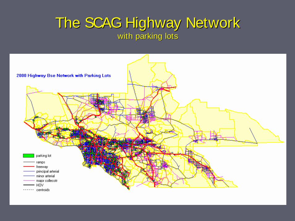
The SCAG Highway Network The SCAG Highway Network with parking lotswith parking lots
START
auto skims for PK
auto skims for OP
transit skims for PK
transit skims for OP
HBW Logsums for PK (mc) HBW Logsums for OP (mc)
trip distribution for PK (gravity) trip distribution for OP (gravity)
mode choice model for PK mode choice model for OP
demand computations (time–of-day model)
auto-truck assignments for AM auto-truck assignments for MD
is the number of outer loops satisfied?
auto-truck assignments for PM auto-truck assignments for NT
transit assignments for AM transit assignments for MD
END
successive average link volume for outer loop of AM
successive average link volume for outer loop of MD
Trip generation
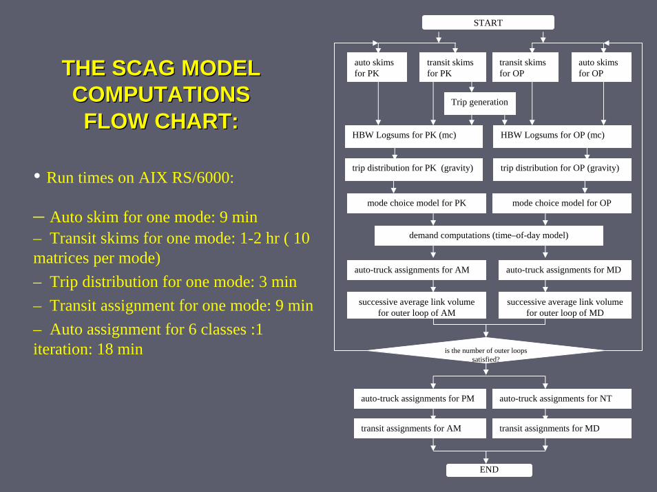
THE SCAG MODEL THE SCAG MODEL COMPUTATIONS COMPUTATIONS FLOW CHART:FLOW CHART:
• Run times on AIX RS/6000:
– Auto skim for one mode: 9 min– Transit skims for one mode: 1-2 hr ( 10 matrices per mode)– Trip distribution for one mode: 3 min– Transit assignment for one mode: 9 min– Auto assignment for 6 classes :1 iteration: 18 min
The SCAG California Model (1997)The SCAG California Model (1997)
►► The next slide shows the convergence of The next slide shows the convergence of both inner iterations of the car assignmentboth inner iterations of the car assignment(in blue) and the outer iterations (in red). (in blue) and the outer iterations (in red). Only 5 iterations were carried out.Only 5 iterations were carried out.
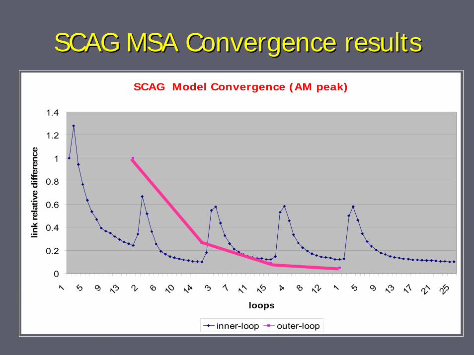
SCAG MSA Convergence resultsSCAG MSA Convergence resultsSCAG Model Convergence (AM peak)
0
0.2
0.4
0.6
0.8
1
1.2
1.4
1 5 9 13 2 6 10 14 3 7 11 15 4 8 12 1 5 9 13 17 21 25
loops
link
rela
tive
diffe
renc
e
inner-loop outer-loop
Comments on the SCAG resultsComments on the SCAG results
►► Each inner loop is so time consuming that the Each inner loop is so time consuming that the number of iterations are limited by the total number of iterations are limited by the total computational time.computational time.
►► Depending on which initial solution is chosen there Depending on which initial solution is chosen there may be 2%may be 2%--5% difference in the resulting VMT 5% difference in the resulting VMT values.values.
►► Convergence is probably very approximate.Convergence is probably very approximate.
Conclusions on Conclusions on ““adad--hochoc”” equilibrationequilibration
►► The The ““adad--hochoc”” equilibration methods do converge equilibration methods do converge empirically.empirically.
►► If the network is congested one may have to If the network is congested one may have to carry out at least 15 iterations and the results may carry out at least 15 iterations and the results may still exhibit 2%still exhibit 2%--5% variation.5% variation.
►► This raises issues about the necessity of very fine This raises issues about the necessity of very fine solutions in the inner loop.solutions in the inner loop.
►► A lot is left to the judgment of the analyst who A lot is left to the judgment of the analyst who carries out the study.carries out the study.
►►Variable demand equilibrium assignmentVariable demand equilibrium assignment
►►MultiMulti--modal models : equilibrationmodal models : equilibration
►►Some large scale applicationsSome large scale applications
►►Stochastic user equilibrium assignmentStochastic user equilibrium assignment
Stochastic user equilibriumStochastic user equilibrium
For each originFor each origin--destination pair of zones, all destination pair of zones, all used routes have equal used routes have equal perceivedperceived travel travel times, and no unused route has a lower times, and no unused route has a lower perceivedperceived travel time.travel time.
►►The models that are used are based on The models that are used are based on various distribution for the perception various distribution for the perception errors: logit, probit, uniformerrors: logit, probit, uniform..
The computational methods usedThe computational methods used
►► The The logitlogit path choice combined with the user path choice combined with the user optimal principle may be formulated as an optimal principle may be formulated as an optimization problem (In the case of constant optimization problem (In the case of constant travel times STOCH by Dial deserves special travel times STOCH by Dial deserves special mention).mention).
►► Hence it may be solved by using a descent Hence it may be solved by using a descent algorithm with well defined convergence algorithm with well defined convergence properties.properties.
►► The The probitprobit path choice requires a solution by path choice requires a solution by Monte Carlo simulation and the use of the MSA Monte Carlo simulation and the use of the MSA method. In this case a convergence proof exists.method. In this case a convergence proof exists.
Uses of Stochastic assignmentUses of Stochastic assignment
►► In relatively unIn relatively un--congested conditions.congested conditions.
►► When congestion dominates the stochastic and When congestion dominates the stochastic and user equilibrium yield similar results.user equilibrium yield similar results.
►► In mildly congested conditions the results may In mildly congested conditions the results may reflect better the paths chosen.reflect better the paths chosen.
►► A nice property of stochastic assignment is that A nice property of stochastic assignment is that the path flows are unique, which is not the case the path flows are unique, which is not the case with deterministic equilibrium assignment.with deterministic equilibrium assignment.
Stochastic assignment Stochastic assignment -- summarysummary
►► The use of stochastic assignment enriches the The use of stochastic assignment enriches the methods used for determining path choice on methods used for determining path choice on lightly congested networks.lightly congested networks.
►► There is no hard and fast rule which may be used There is no hard and fast rule which may be used to determine when stochastic assignment should to determine when stochastic assignment should be used. It is up to the analyst that carries out the be used. It is up to the analyst that carries out the study.study.