worksheets for mathematics ii
TRANSCRIPT

Worksheets for Mathematics IIJana Volná, Petr Volný
Introduction
The study material is designed for students of VSB - Technical University of Ostrava.
The worksheets consist of several theoretical sheets, some solved problems and some sheets with unsolved problems for practicing. The materialsshould support classwork and they are not recommended for self-study or as a replacement for textbooks.
The worksheets are based on MORÁVKOVÁ, Z., PALÁCEK, R., SCHREIBEROVÁ, P., VOLNÝ, P.: Matematika II: Pracovní listy. Ostrava: VŠB -Technická univerzita Ostrava, 2014. ISBN 978-80-248-3324-8 (in Czech).
Thanks
Technology for the Future 2.0, CZ.02.2.69/0.0/0.0/18_058/0010212
ISBN 978-80-248-4511-1DOI 10.31490/9788024845111

Contents
Integral calculus of functions of one real variable 4Indefinite integrals, antiderivatives . . . . . . . . . . . . . . . . . 5Properties . . . . . . . . . . . . . . . . . . . . . . . . . . . . . . . 6Elementary integrals . . . . . . . . . . . . . . . . . . . . . . . . . 7Direct method of integration . . . . . . . . . . . . . . . . . . . . . 8Integration by parts . . . . . . . . . . . . . . . . . . . . . . . . . . 16Integration by substitution . . . . . . . . . . . . . . . . . . . . . . 23Rational functions . . . . . . . . . . . . . . . . . . . . . . . . . . . 33Trigonometric functions . . . . . . . . . . . . . . . . . . . . . . . 46Irrational functions . . . . . . . . . . . . . . . . . . . . . . . . . . 57Definite integrals, geometric interpretation . . . . . . . . . . . . 62Definite integrals, definition . . . . . . . . . . . . . . . . . . . . . 63Definite integrals, properties . . . . . . . . . . . . . . . . . . . . . 64Integration by parts and substitution . . . . . . . . . . . . . . . . 69Definite integrals, rational functions . . . . . . . . . . . . . . . . 76Improper integral of the first kind . . . . . . . . . . . . . . . . . . 78Improper integral of the second kind . . . . . . . . . . . . . . . . 81Geometrical application, area of planar regions . . . . . . . . . . 84Length of planar curves . . . . . . . . . . . . . . . . . . . . . . . 96Volume of solids of revolution . . . . . . . . . . . . . . . . . . . . 102Lateral surface of solids of revolution . . . . . . . . . . . . . . . . 111Physical applications . . . . . . . . . . . . . . . . . . . . . . . . . 116
Differential calculus of functions of two real variables 125Functions of two real variables, domains . . . . . . . . . . . . . . 126Functions of two real variables, graphs . . . . . . . . . . . . . . . 139Contour lines . . . . . . . . . . . . . . . . . . . . . . . . . . . . . 140Limits, continuity . . . . . . . . . . . . . . . . . . . . . . . . . . . 144Partial derivatives . . . . . . . . . . . . . . . . . . . . . . . . . . . 147Differentials . . . . . . . . . . . . . . . . . . . . . . . . . . . . . . 157Tangent plane, normal line, Taylor polynomial . . . . . . . . . . 165Implicit functions . . . . . . . . . . . . . . . . . . . . . . . . . . . 172Local extrema . . . . . . . . . . . . . . . . . . . . . . . . . . . . . 180Constraint extrema . . . . . . . . . . . . . . . . . . . . . . . . . . 188Global extrema . . . . . . . . . . . . . . . . . . . . . . . . . . . . 194
Ordinary differential equations 198Differential equations of the n-th order . . . . . . . . . . . . . . . 199First order ordinary differential equations . . . . . . . . . . . . . 201Slope field . . . . . . . . . . . . . . . . . . . . . . . . . . . . . . . 202Cauchy problem . . . . . . . . . . . . . . . . . . . . . . . . . . . . 203Separable differential equations . . . . . . . . . . . . . . . . . . . 204Linear differential equations of the first order . . . . . . . . . . . 220Linear differential equations of the second order with constant
coefficients . . . . . . . . . . . . . . . . . . . . . . . . . . . . 226Linearly independent functions . . . . . . . . . . . . . . . . . . . 227Characteristic equation . . . . . . . . . . . . . . . . . . . . . . . . 228Non-homogeneous second order LODE - solution . . . . . . . . 232Variation of constants . . . . . . . . . . . . . . . . . . . . . . . . . 233Undetermined coefficients . . . . . . . . . . . . . . . . . . . . . . 239

Worksheets for Mathematics II
Integral calculus of functions of one real variable
Worksheets for Mathematics II
5 – Indefinite integrals, antiderivatives Ry
In the calculus of functions depending on one real variable we met veryimportant objects, derivatives of functions. We assigned to every functionf (x) the new one, f ′(x). The preceding task has changed, now we try tofind to every function f (x) a function F(x) such that F′(x) = f (x). There isa question. Which function do I need to differentiate to get original givenfunction f (x)?
Definition
Let a function f (x) is defined on an open interval I. The function F(x)is called antiderivative of the function f (x) on I if it holds F′(x) = f (x)for every x ∈ I.
Theorem
Let the function F(x) is antiderivative of f (x) on I, then any other an-tiderivative of the function f (x) on I can be written in the form F(x)+ c,where constant c ∈ R.
Remark
If an antiderivative does exist, there are infinitely many antiderivativeswhich differ only by a constant c. We know that if one construct tangentline at a point x to a given function, the derivative evaluated at this pointis slope of this tangent line. The graphs of antiderivatives are displacedparallel in the direction of the y-axis. Tangent lines to graphs at thegiven points x are parallel (they have the same slope), i.e. they have thesame derivative.
Worksheets for Mathematics II
6 – Indefinite integrals, definition, properties Ry
Definition
The set of all antiderivatives of the function f (x) on I is called indefinite
integral of the function f (x) an is denoted by∫
f (x)dx. Thus,
∫f (x)dx = F(x) + c, x ∈ I.
Remark
• The function f (x) is called integrand.
• The expression dx is differential of x, for simplicity, it gives us in-formation about the name of independent variable. The meaningof this object will be discussed later.
• The number c is called constant of integration.
Properties:
Theorem
To every function y = f (x) continuous on the interval I there exists
indefinite integral∫
f (x)dx which is again a continuous function on I.
The following very important theorem represents key properties whichare necessary for elementary calculations of indefinite integrals.
Theorem
If there exist two integrals∫
f (x)dx and∫
g(x)dx on I, then there also
exist the integrals of their sum, difference and multiple of the constant,∫( f (x)± g(x)) dx =
∫f (x)dx±
∫g(x)dx∫
k · f (x)dx = k∫
f (x)dx, k ∈ R.
Worksheets for Mathematics II
7 – Elementary integrals, formulas Ry
1.∫
0 dx = c
2.∫
xn dx =xn+1
n + 1+ c, n 6= −1, x > 0
3.∫
ex dx = ex + c
4.∫
ax dx =ax
ln a+ c, a > 0, a 6= 1
5.∫ 1
xdx = ln |x|+ c, x 6= 0
6.∫
sin x dx = − cos x + c
7.∫
cos x dx = sin x + c
8.∫ 1
cos2 xdx = tan x + c, x 6= (2k + 1)
π
2
9.∫ 1
sin2 xdx = − cot x + c, x 6= kπ
10.∫ 1√
1− x2dx = arcsin x + c, |x| < 1
11.∫ 1
1 + x2 dx = arctan x + c
12.∫ f ′(x)
f (x)dx = ln | f (x)|+ c, f (x) 6= 0
13.∫
f (ax + b)dx =1a
F(ax + b) + c, a 6= 0
13a.∫
(ax + b)n dx =1a(ax + b)n+1
n + 1+ c, a 6= 0
13b.∫
eax+b dx =1a
eax+b + c, a 6= 0
13c.∫ 1
ax + bdx =
1a
ln |ax + b|+ c, a 6= 0
13d.∫
sin(ax + b)dx = −1a
cos(ax + b) + c, a 6= 0
13e.∫
cos(ax + b)dx =1a
sin(ax + b) + c, a 6= 0
13f.∫ 1
cos2(ax)dx =
1a
tan(ax) + c, ax 6= (2k + 1)π
2, a 6= 0
13g.∫ 1
sin2(ax)dx = −1
acot(ax) + c, ax 6= kπ, a 6= 0
13h.∫ 1√
d2 − x2dx = arcsin
xd+ c,
∣∣∣xd
∣∣∣ < 1, d 6= 0
13i.∫ 1
d2 + x2 dx =1d
arctanxd+ c, d 6= 0

Worksheets for Mathematics II
8 – Direct method of integration Ry
Example
Calculate the integral∫ (
7 3√x2 +12
sin x− 21 + x2
)dx.
We need to integrate the sum of functions, thus the condition 14 must be applied. We get the sum of threeintegrals, ∫
7 3√x2 dx +∫ 1
2sin x dx−
∫ 21 + x2 dx.
Constants can be factored out from the single integrals using formula 15 and the function 3√x2 one can rewriteas x
23 ,
7∫
x23 dx +
12
∫sin x dx− 2
∫ 11 + x2 dx.
Finally, we can find appropriate antiderivatives using formulas 2, 6 and 11.
Result:∫ (7 3√x2 +
12
sin x− 21 + x2
)dx = 7
x53
53− 1
2cos x− 2 arctan x + c =
215
3√x5 − 12
cos x− 2 arctan x + c.
Hints
1.∫
0 dx = c
2.∫
xn dx =xn+1
n + 1+ c
3.∫
ex dx = ex + c
4.∫
ax dx =ax
ln a+ c
5.∫ 1
xdx = ln |x|+ c
6.∫
sin x dx = − cos x + c
7.∫
cos x dx = sin x + c
8.∫ 1
cos2 xdx = tan x + c
9.∫ 1
sin2 xdx = − cot x + c
10.∫ 1√
1− x2dx = arcsin x + c
11.∫ 1
1 + x2 dx = arctan x + c
12.∫ f ′(x)
f (x)dx = ln | f (x)|+ c
13.∫
f (ax+b)dx =1a
F(ax+b) + c
f = f (x) g = g(x)
14.∫
( f ± g)dx =∫
f dx±∫
g dx
15.∫
(k · f )dx = k∫
f dx, k ∈ R

Worksheets for Mathematics II
9 – Direct method of integration Ry
Example
Calculate the integral∫ (e2x − 1
ex + 1+
41− cos2 x
)dx.
Let us divide our integral into the sum of two integrals using formula 14,∫ e2x − 1ex + 1
dx +∫ 4
1− cos2 xdx.
For the integration of the first integral is necessary to use the formula a2 − b2 = (a− b)(a + b), i.e.∫ e2x − 1ex + 1
dx =∫
(ex)2 − 1ex + 1
dx =∫
(ex − 1)(ex + 1)ex + 1
dx =∫
(ex − 1)dx = ex − x + c.
For the second integral using formulas 15 and 9 and trigonometric formula sin2 x + cos2 x = 1 we get∫ 41− cos2 x
dx = 4∫ 1
sin2 xdx = −4 cot x + c.
Result: ∫ (e2x − 1ex + 1
+4
1− cos2 x
)dx = ex − x− 4 cot x + c.
Hints
1.∫
0 dx = c
2.∫
xn dx =xn+1
n + 1+ c
3.∫
ex dx = ex + c
4.∫
ax dx =ax
ln a+ c
5.∫ 1
xdx = ln |x|+ c
6.∫
sin x dx = − cos x + c
7.∫
cos x dx = sin x + c
8.∫ 1
cos2 xdx = tan x + c
9.∫ 1
sin2 xdx = − cot x + c
10.∫ 1√
1− x2dx = arcsin x + c
11.∫ 1
1 + x2 dx = arctan x + c
12.∫ f ′(x)
f (x)dx = ln | f (x)|+ c
13.∫
f (ax+b)dx =1a
F(ax+b) + c
f = f (x) g = g(x)
14.∫
( f ± g)dx =∫
f dx±∫
g dx
15.∫
(k · f )dx = k∫
f dx, k ∈ R
Worksheets for Mathematics II
10 – Direct method of integration Ry
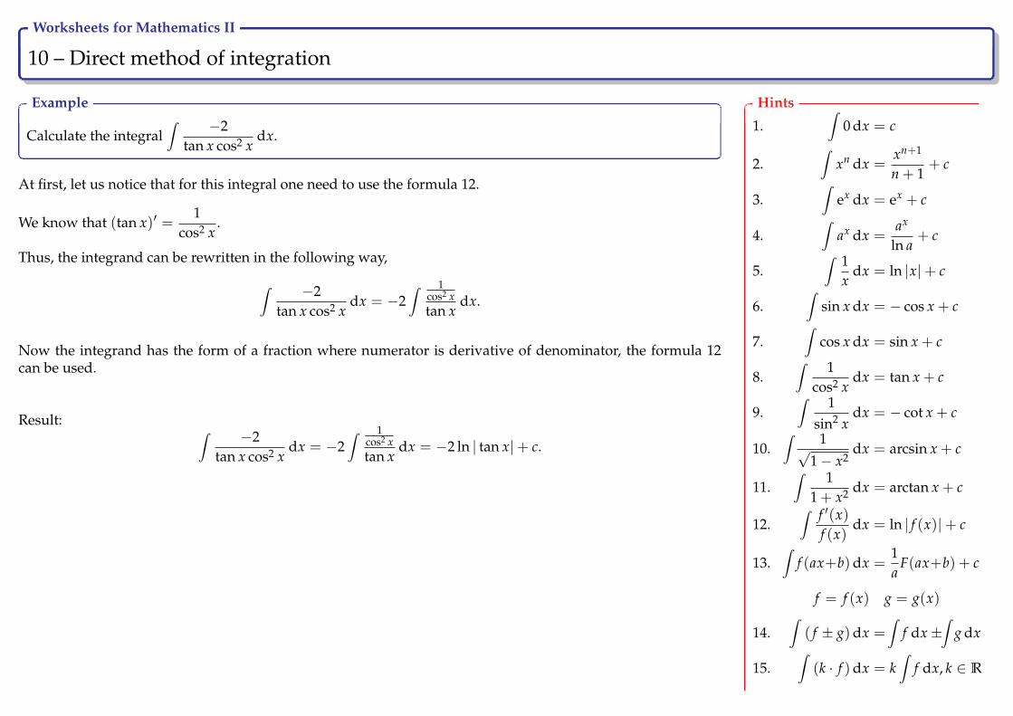
Example
Calculate the integral∫ −2
tan x cos2 xdx.
At first, let us notice that for this integral one need to use the formula 12.
We know that (tan x)′ =1
cos2 x.
Thus, the integrand can be rewritten in the following way,
∫ −2tan x cos2 x
dx = −2∫ 1
cos2 xtan x
dx.
Now the integrand has the form of a fraction where numerator is derivative of denominator, the formula 12can be used.
Result: ∫ −2tan x cos2 x
dx = −2∫ 1
cos2 xtan x
dx = −2 ln | tan x|+ c.
Hints
1.∫
0 dx = c
2.∫
xn dx =xn+1
n + 1+ c
3.∫
ex dx = ex + c
4.∫
ax dx =ax
ln a+ c
5.∫ 1
xdx = ln |x|+ c
6.∫
sin x dx = − cos x + c
7.∫
cos x dx = sin x + c
8.∫ 1
cos2 xdx = tan x + c
9.∫ 1
sin2 xdx = − cot x + c
10.∫ 1√
1− x2dx = arcsin x + c
11.∫ 1
1 + x2 dx = arctan x + c
12.∫ f ′(x)
f (x)dx = ln | f (x)|+ c
13.∫
f (ax+b)dx =1a
F(ax+b) + c
f = f (x) g = g(x)
14.∫
( f ± g)dx =∫
f dx±∫
g dx
15.∫
(k · f )dx = k∫
f dx, k ∈ R

Worksheets for Mathematics II
11 – Direct method of integration Ry
Example
Calculate the integrals∫
e−3x+1 dx,∫ 1√
4− (3x− 1)2dx.
Solution for the integral∫
e−3x+1 dx.
Integrand is of the form eax+b, then we use linear substitution, the formula 13b, where a = −3,b = 1. We can directly find an antiderivative .
Result: ∫e−3x+1 dx = −1
3e−3x+1 + c.
Solution for the integral∫ 1√
4− (3x− 1)2dx.
The integrand is of the form1√
d2 − (ax + b)2, then we use the formulas 13 and 13h, where
a = 3, b = −1, d = 2.
Result: ∫ 1√4− (3x− 1)2
dx =13
arcsin3x− 1
2+ c.
Let us note that formulas 13a-13i are direct consequences of the formula 1. This formula representslinear substitution ax + b = t.
HintsLinear substitution, general formulas
13.∫
f (ax + b)dx =1a
F(ax + b) + c
13a.∫
(ax + b)n dx =1a(ax + b)n+1
n + 1+ c
13b.∫
eax+b dx =1a
eax+b + c
13c.∫ 1
ax + bdx =
1a
ln |ax + b|+ c
13d.∫
sin(ax + b)dx = −1a
cos(ax + b) + c
13e.∫
cos(ax + b)dx =1a
sin(ax + b) + c
13f.∫ 1
cos2(ax)dx =
1a
tan(ax) + c
13g.∫ 1
sin2(ax)dx = −1
acot(ax) + c
13h.∫ 1√
d2 − x2dx = arcsin
xd+ c
13i.∫ 1
d2 + x2 dx =1d
arctanxd+ c

Worksheets for Mathematics II
12 – Direct method of integration Ry
Exercise
Solve:
a)∫ (
x5 − 2x +x2
3
)dx b)
∫ (√x + 4√
x)
dx c)∫ 2x− 1√
xdx d)
∫ 3x
dx
Hints
1.∫
0 dx = c
2.∫
xn dx =xn+1
n + 1+ c
3.∫
ex dx = ex + c
4.∫
ax dx =ax
ln a+ c
5.∫ 1
xdx = ln |x|+ c
6.∫
sin x dx = − cos x + c
7.∫
cos x dx = sin x + c
8.∫ 1
cos2 xdx = tan x + c
9.∫ 1
sin2 xdx = − cot x + c
10.∫ 1√
1− x2dx = arcsin x + c
11.∫ 1
1 + x2 dx = arctan x + c
12.∫ f ′(x)
f (x)dx = ln | f (x)|+ c
13.∫
f (ax+b)dx =1a
F(ax+b) + c
f = f (x) g = g(x)
14.∫
( f ± g)dx =∫
f dx±∫
g dx
15.∫
(k · f )dx = k∫
f dx, k ∈ R
Worksheets for Mathematics II
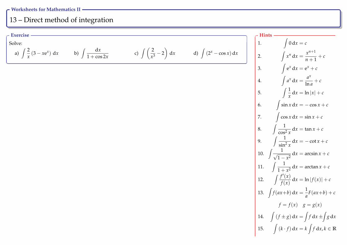
13 – Direct method of integration Ry
Exercise
Solve:
a)∫ 2
x(3− xex) dx b)
∫ dx1 + cos 2x
c)∫ ( 2
x3 − 2)
dx d)∫
(2x − cos x)dx
Hints
1.∫
0 dx = c
2.∫
xn dx =xn+1
n + 1+ c
3.∫
ex dx = ex + c
4.∫
ax dx =ax
ln a+ c
5.∫ 1
xdx = ln |x|+ c
6.∫
sin x dx = − cos x + c
7.∫
cos x dx = sin x + c
8.∫ 1
cos2 xdx = tan x + c
9.∫ 1
sin2 xdx = − cot x + c
10.∫ 1√
1− x2dx = arcsin x + c
11.∫ 1
1 + x2 dx = arctan x + c
12.∫ f ′(x)
f (x)dx = ln | f (x)|+ c
13.∫
f (ax+b)dx =1a
F(ax+b) + c
f = f (x) g = g(x)
14.∫
( f ± g)dx =∫
f dx±∫
g dx
15.∫
(k · f )dx = k∫
f dx, k ∈ R
Worksheets for Mathematics II
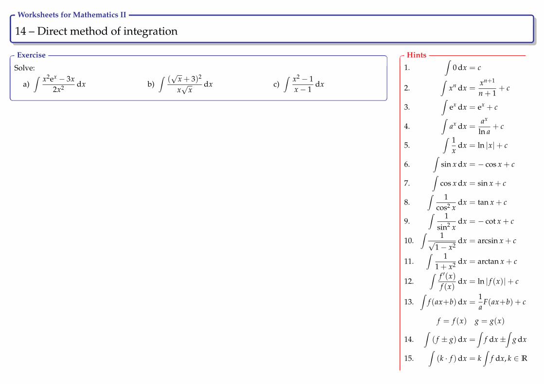
14 – Direct method of integration Ry
Exercise
Solve:
a)∫ x2ex − 3x
2x2 dx b)∫
(√
x + 3)2
x√
xdx c)
∫ x2 − 1x− 1
dx
Hints
1.∫
0 dx = c
2.∫
xn dx =xn+1
n + 1+ c
3.∫
ex dx = ex + c
4.∫
ax dx =ax
ln a+ c
5.∫ 1
xdx = ln |x|+ c
6.∫
sin x dx = − cos x + c
7.∫
cos x dx = sin x + c
8.∫ 1
cos2 xdx = tan x + c
9.∫ 1
sin2 xdx = − cot x + c
10.∫ 1√
1− x2dx = arcsin x + c
11.∫ 1
1 + x2 dx = arctan x + c
12.∫ f ′(x)
f (x)dx = ln | f (x)|+ c
13.∫
f (ax+b)dx =1a
F(ax+b) + c
f = f (x) g = g(x)
14.∫
( f ± g)dx =∫
f dx±∫
g dx
15.∫
(k · f )dx = k∫
f dx, k ∈ R

Worksheets for Mathematics II
15 – Direct method of integration Ry
Exercise
Solve:
a)∫ sin 2x
sin2 xdx b)
∫ −41 + x2 dx c)
∫ 2√1− x2
dx
Hints
1.∫
0 dx = c
2.∫
xn dx =xn+1
n + 1+ c
3.∫
ex dx = ex + c
4.∫
ax dx =ax
ln a+ c
5.∫ 1
xdx = ln |x|+ c
6.∫
sin x dx = − cos x + c
7.∫
cos x dx = sin x + c
8.∫ 1
cos2 xdx = tan x + c
9.∫ 1
sin2 xdx = − cot x + c
10.∫ 1√
1− x2dx = arcsin x + c
11.∫ 1
1 + x2 dx = arctan x + c
12.∫ f ′(x)
f (x)dx = ln | f (x)|+ c
13.∫
f (ax+b)dx =1a
F(ax+b) + c
f = f (x) g = g(x)
14.∫
( f ± g)dx =∫
f dx±∫
g dx
15.∫
(k · f )dx = k∫
f dx, k ∈ R

Worksheets for Mathematics II
16 – Integration by parts Ry
If we integrate a sum or a difference of functions, we simply need tointegrate every summand separately. But this is not true for multiplicationof functions, ∫
f (x) · g(x)dx 6=∫
f (x)dx ·∫
g(x)dx.
There is a natural question, is there any way how to integrate multipli-cation of functions? Let us recall how to differentiate multiplication offunctions,
(u · v)′ = u′ · v + u · v′ ⇒ u · v′ = (u · v)′ − u′ · v.
After integration we get∫u · v′ dx = u · v−
∫u′ · v dx.
Theorem
Let the functions u(x) and v(x) have continuous derivatives on the in-terval I, then∫
u(x) · v′(x)dx = u(x) · v(x)−∫
u′(x) · v(x)dx.
The method is called integration by parts.
Note that the alternative expression∫u′(x) · v(x)dx = u(x) · v(x)−
∫u(x) · v′(x)dx
represents the same formula for integration by parts method.
The point is to consider a multiplication of two functions in such a waythat one factor must be differentiated and the second one integrated. Theintegration is not complete because we replace the original integral by thenew one. But the new integral is usually simpler from the point of view ofthe integration and quite often it can be directly integrated.
Worksheets for Mathematics II
17 – Integration by parts Ry
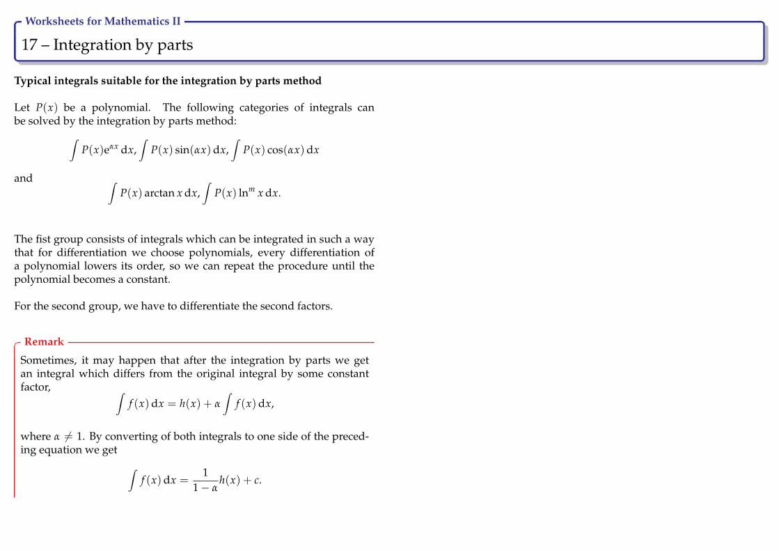
Typical integrals suitable for the integration by parts method
Let P(x) be a polynomial. The following categories of integrals canbe solved by the integration by parts method:∫
P(x)eαx dx,∫
P(x) sin(αx)dx,∫
P(x) cos(αx)dx
and ∫P(x) arctan x dx,
∫P(x) lnm x dx.
The fist group consists of integrals which can be integrated in such a waythat for differentiation we choose polynomials, every differentiation ofa polynomial lowers its order, so we can repeat the procedure until thepolynomial becomes a constant.
For the second group, we have to differentiate the second factors.
Remark
Sometimes, it may happen that after the integration by parts we getan integral which differs from the original integral by some constantfactor, ∫
f (x)dx = h(x) + α∫
f (x)dx,
where α 6= 1. By converting of both integrals to one side of the preced-ing equation we get ∫
f (x)dx =1
1− αh(x) + c.

Worksheets for Mathematics II
18 – Integration by parts Ry
Example
Calculate the integral∫
(−2x + 3) cos 3x dx.
The integral is of the form∫
P(x) cos ax dx, thus we use integration by parts method, where the polynomial
P(x) is differentiated and the function cos ax is integrated.
u = −2x + 3 v′ = cos 3x
u′ = −2 v =13
sin 3x
We get ∫(−2x + 3) cos 3x dx =
−2x + 33
sin 3x−∫ −2
3sin 3x dx =
−2x + 33
sin 3x +23
∫sin 3x dx.
We get simpler integral∫
sin 3x dx, which can be directly integrated,∫sin 3x dx = −1
3cos 3x + c.
Result: ∫(−2x + 3) cos 3x dx =
−2x + 33
sin 3x− 29
cos 3x + c.
Hints
Integration by parts
u = u(x) v′ = v′(x)u′ = u′(x) v = v(x)
∫u · v′ dx = u · v−
∫u′ · v dx
Worksheets for Mathematics II
19 – Integration by parts Ry
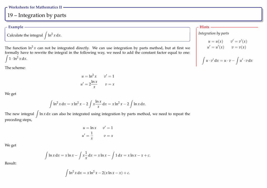
Example
Calculate the integral∫
ln2 x dx.
The function ln2 x can not be integrated directly. We can use integration by parts method, but at first weformally have to rewrite the integral in the following way, we need to add the constant factor equal to one:∫
1 · ln2 x dx.
The scheme:
u = ln2 x v′ = 1
u′ = 2ln x
xv = x
We get ∫ln2 x dx = x ln2 x− 2
∫x
ln xx
dx = x ln2 x− 2∫
ln x dx.
The new integral∫
ln x dx can also be integrated using integration by parts method, we need to repeat the
preceding steps,
u = ln x v′ = 1
u′ =1x
v = x
We get ∫ln x dx = x ln x−
∫x
1x
dx = x ln x−∫
1 dx = x ln x− x + c.
Result: ∫ln2 x dx = x ln2 x− 2(x ln x− x) + c.
Hints
Integration by parts
u = u(x) v′ = v′(x)u′ = u′(x) v = v(x)
∫u · v′ dx = u · v−
∫u′ · v dx
Worksheets for Mathematics II
20 – Integration by parts Ry
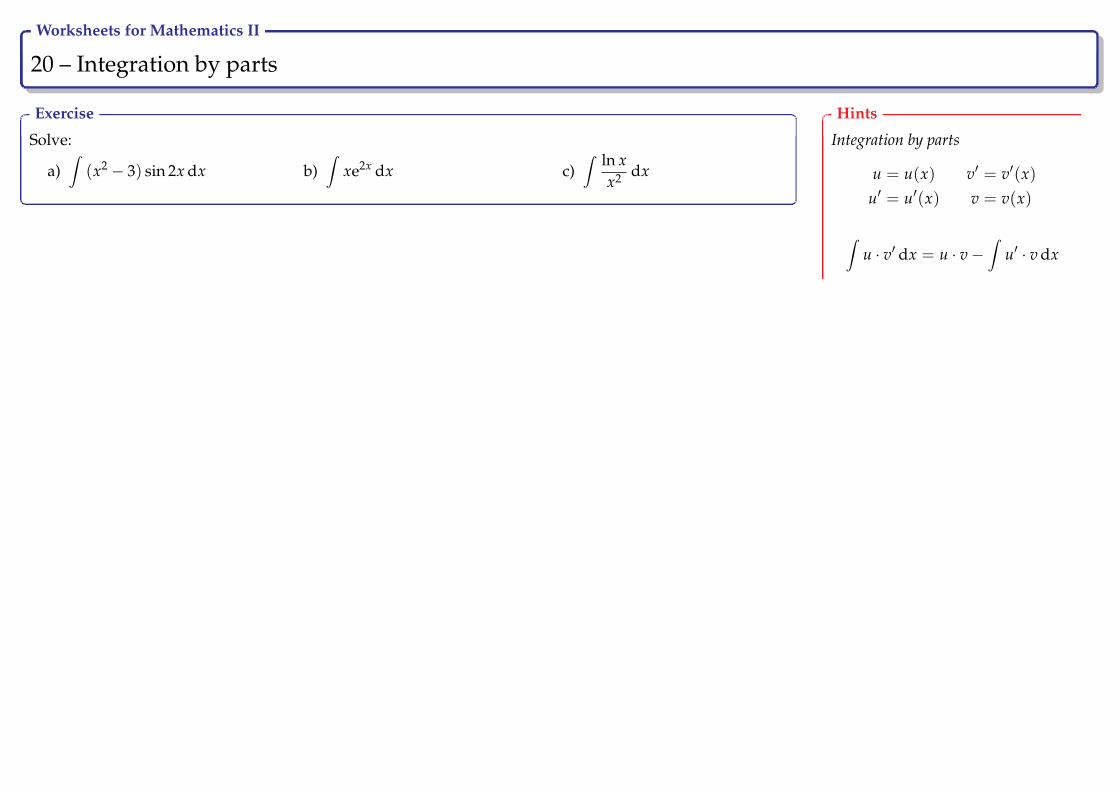
Exercise
Solve:
a)∫
(x2 − 3) sin 2x dx b)∫
xe2x dx c)∫ ln x
x2 dx
Hints
Integration by parts
u = u(x) v′ = v′(x)u′ = u′(x) v = v(x)
∫u · v′ dx = u · v−
∫u′ · v dx
Worksheets for Mathematics II
21 – Integration by parts Ry
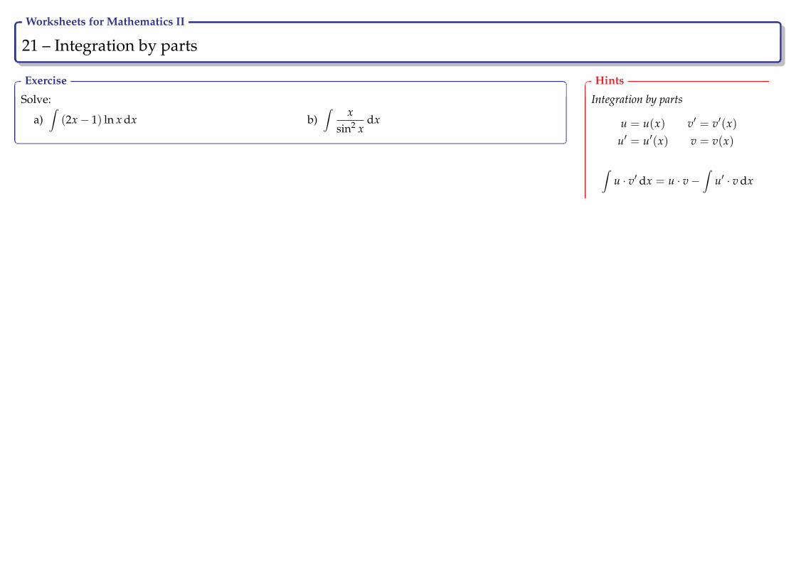
Exercise
Solve:
a)∫
(2x− 1) ln x dx b)∫ x
sin2 xdx
Hints
Integration by parts
u = u(x) v′ = v′(x)u′ = u′(x) v = v(x)
∫u · v′ dx = u · v−
∫u′ · v dx

Worksheets for Mathematics II
22 – Integration by parts Ry
Exercise
Solve:
a)∫
ex sin x dx b)∫
cos(ln x)dx
Hints
Integration by parts
u = u(x) v′ = v′(x)u′ = u′(x) v = v(x)
∫u · v′ dx = u · v−
∫u′ · v dx
Integration by parts - special case∫f (x)dx = h(x) + α ·
∫f (x)dx, α 6= 1
⇒∫
f (x)dx =h(x)1− α
+ c
Worksheets for Mathematics II
23 – Integration by substitution Ry
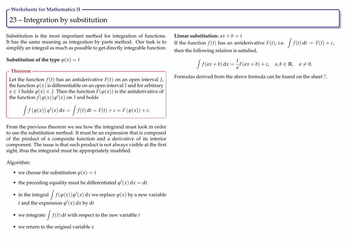
Substitution is the most important method for integration of functions.It has the same meaning as integration by parts method. Our task is tosimplify an integral as much as possible to get directly integrable function.
Substitution of the type ϕ(x) = t
Theorem
Let the function f (t) has an antiderivative F(t) on an open interval J,the function ϕ(x) is differentiable on an open interval I and for arbitraryx ∈ I holds ϕ(x) ∈ J. Then the function F(ϕ(x)) is the antiderivative ofthe function f (ϕ(x))ϕ′(x) on I and holds∫
f (ϕ(x)) ϕ′(x)dx =∫
f (t)dt = F(t) + c = F (ϕ(x)) + c.
From the previous theorem we see how the integrand must look in orderto use the substitution method. It must be an expression that is composedof the product of a composite function and a derivative of its interiorcomponent. The issue is that such product is not always visible at the firstsight, thus the integrand must be appropriately modified.
Algorithm:
• we choose the substitution ϕ(x) = t
• the preceding equality must be differentiated ϕ′(x)dx = dt
• in the integral∫
f (ϕ(x))ϕ′(x)dx we replace ϕ(x) by a new variable
t and the expression ϕ′(x)dx by dt
• we integrate∫
f (t)dt with respect to the new variable t
• we return to the original variable x
Linear substitution: ax + b = tIf the function f (t) has an antiderivative F(t), i.e.
∫f (t)dt = F(t) + c,
then the following relation is satisfied,∫f (ax + b)dx =
1a
F(ax + b) + c, a, b ∈ R, a 6= 0.
Formulas derived from the above formula can be found on the sheet 7.
Worksheets for Mathematics II
24 – Integration by substitution Ry
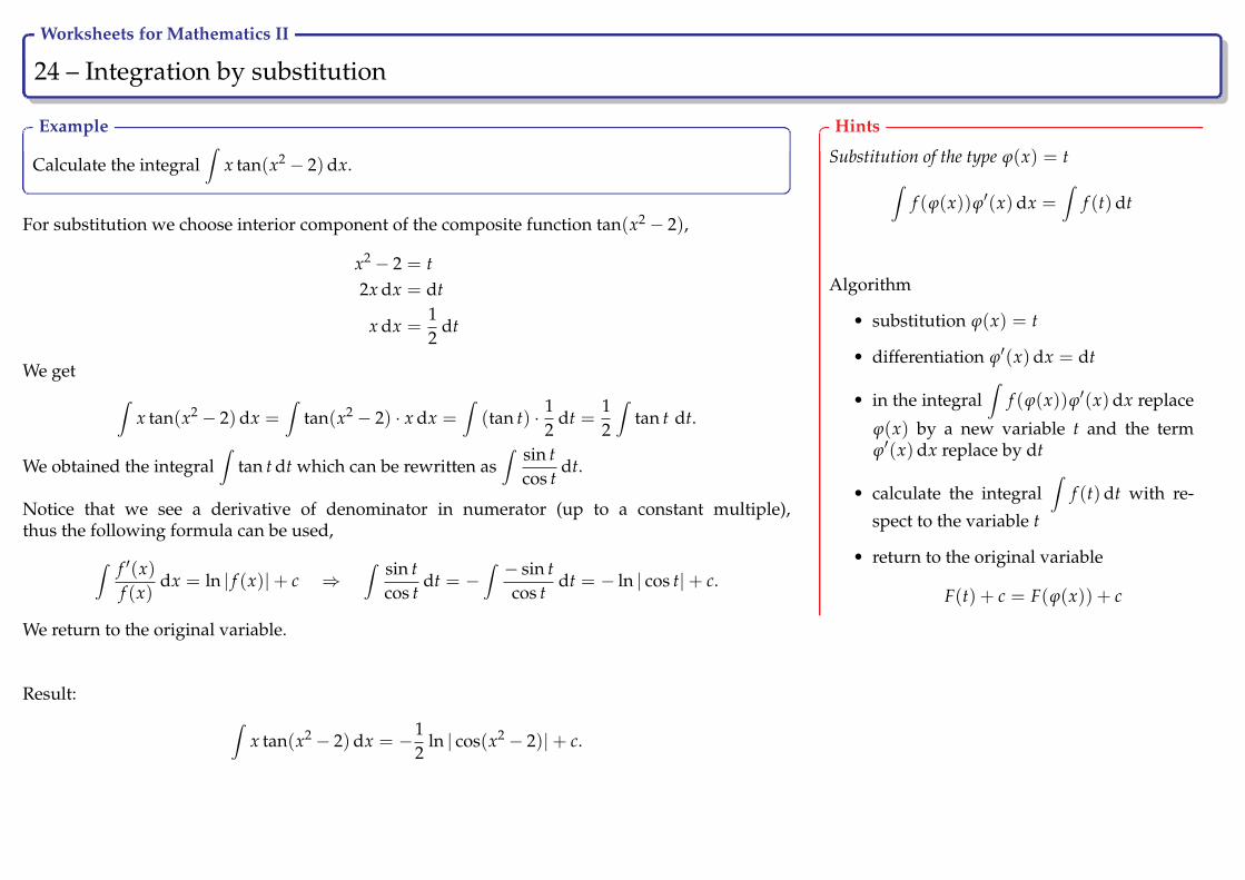
Example
Calculate the integral∫
x tan(x2 − 2)dx.
For substitution we choose interior component of the composite function tan(x2 − 2),
x2 − 2 = t2x dx = dt
x dx =12
dt
We get ∫x tan(x2 − 2)dx =
∫tan(x2 − 2) · x dx =
∫(tan t) · 1
2dt =
12
∫tan t dt.
We obtained the integral∫
tan t dt which can be rewritten as∫ sin t
cos tdt.
Notice that we see a derivative of denominator in numerator (up to a constant multiple),thus the following formula can be used,∫ f ′(x)
f (x)dx = ln | f (x)|+ c ⇒
∫ sin tcos t
dt = −∫ − sin t
cos tdt = − ln | cos t|+ c.
We return to the original variable.
Result: ∫x tan(x2 − 2)dx = −1
2ln | cos(x2 − 2)|+ c.
Hints
Substitution of the type ϕ(x) = t∫f (ϕ(x))ϕ′(x)dx =
∫f (t)dt
Algorithm
• substitution ϕ(x) = t
• differentiation ϕ′(x)dx = dt
• in the integral∫
f (ϕ(x))ϕ′(x)dx replace
ϕ(x) by a new variable t and the termϕ′(x)dx replace by dt
• calculate the integral∫
f (t)dt with re-
spect to the variable t
• return to the original variable
F(t) + c = F(ϕ(x)) + c

Worksheets for Mathematics II
25 – Integration by substitution Ry
Example
Calculate the integral∫ arcsin x√
1− x2dx.
We choose the substitution
arcsin x = t1√
1− x2dx = dt
We get ∫arcsin x
1√1− x2
dx =∫
t dt.
We obtain an elementary integral which can be directly integrated,∫t dt =
t2
2+ c.
We return to the original variable.
Result: ∫ arcsin x√1− x2
dx =arcsin2 x
2+ c.
Hints
Substitution of the type ϕ(x) = t∫f (ϕ(x))ϕ′(x)dx =
∫f (t)dt
Algorithm
• substitution ϕ(x) = t
• differentiation ϕ′(x)dx = dt
• in the integral∫
f (ϕ(x))ϕ′(x)dx replace
ϕ(x) by a new variable t and the termϕ′(x)dx replace by dt
• calculate the integral∫
f (t)dt with re-
spect to the variable t
• return to the original variable
F(t) + c = F(ϕ(x)) + c
Worksheets for Mathematics II
26 – Integration by substitution Ry
Exercise
Solve:
a)∫ dx
(x2 + 1)√
arctan xb)∫
ex cos(ex)dx
Hints
Substitution of the type ϕ(x) = t∫f (ϕ(x))ϕ′(x)dx =
∫f (t)dt
Algorithm
• substitution ϕ(x) = t
• differentiation ϕ′(x)dx = dt
• in the integral∫
f (ϕ(x))ϕ′(x)dx replace
ϕ(x) by a new variable t and the termϕ′(x)dx replace by dt
• calculate the integral∫
f (t)dt with re-
spect to the variable t
• return to the original variable
F(t) + c = F(ϕ(x)) + c
Worksheets for Mathematics II
27 – Integration by substitution Ry
Exercise
Solve:
a)∫
x cot(1 + x2)dx b)∫
(3 + ln x)5
xdx
Hints
Substitution of the type ϕ(x) = t∫f (ϕ(x))ϕ′(x)dx =
∫f (t)dt
Algorithm
• substitution ϕ(x) = t
• differentiation ϕ′(x)dx = dt
• in the integral∫
f (ϕ(x))ϕ′(x)dx replace
ϕ(x) by a new variable t and the termϕ′(x)dx replace by dt
• calculate the integral∫
f (t)dt with re-
spect to the variable t
• return to the original variable
F(t) + c = F(ϕ(x)) + c
Worksheets for Mathematics II
28 – Integration by substitution Ry
Exercise
Solve:
a)∫ tan x
cos2 xdx b)
∫x2e−x3
dx
Hints
Substitution of the type ϕ(x) = t∫f (ϕ(x))ϕ′(x)dx =
∫f (t)dt
Algorithm
• substitution ϕ(x) = t
• differentiation ϕ′(x)dx = dt
• in the integral∫
f (ϕ(x))ϕ′(x)dx replace
ϕ(x) by a new variable t and the termϕ′(x)dx replace by dt
• calculate the integral∫
f (t)dt with re-
spect to the variable t
• return to the original variable
F(t) + c = F(ϕ(x)) + c

Worksheets for Mathematics II
29 – Integration by substitution Ry
Substitution of the type x = ϕ(t)
From the preceding substitution category follows that we rewrite
the integral∫
f (ϕ(x)) ϕ′(x)dx by means of the substitution ϕ(x) = t on
the integral with a new variable∫
f (t)dt. Sometimes, it is necessary to
choose a different approach and replace the original variable by a new
function. Consider that we have to calculate the integral∫
f (x)dx. By
means of the substitution x = ϕ(t) and dx = ϕ′(t)dt we try to replace the
integral by a new integral∫
f (ϕ(t)) ϕ′(t)dt. To find an antiderivative,
the following must be satisfied:
• f (x) is continuous on (a, b)
• x = ϕ(t) is strictly monotonic on (α, β) and ϕ′(t) 6= 0 is continuouson (α, β).
If both assumptions are fulfilled, then the inverse function ϕ−1(x) 6= 0exists and t = ϕ−1(x).
Theorem
Let a function f (x) be continuous on an interval J, let a strictly mono-tonic function ϕ(t) have a derivative on I not equal to zero for ev-ery t ∈ I and let it hold ϕ(I) = J. Then f (x) has an antiderivativeF(
ϕ−1(x))
on J and it holds
∫f (x)dx =
∫f (ϕ(t))ϕ′(t)dt = F
(ϕ−1(x)
)+ c.
By means of the substitution method we usually integrate irrational func-tions.
• Integrand contains the expression n√
ax + b. We choose the followingsubstitutions ax + b = tn and dx = ntn−1 dt.
• If the integrand consists of irrational functions with different rootsn1√
ax + b, n2√
ax + b, ..., we choose the substitution ax+ b = tn, wheren is the least common multiple of the numbers n1, n2, ....
• Integrand contains the expression√
a2 − b2x2. The substitution iscalled trigonometric because we set bx = a sin t or bx = a cos t, i.e.dx =
ab
cos t dt or dx = − ab
sin t dt.
Worksheets for Mathematics II
30 – Integration by substitution Ry
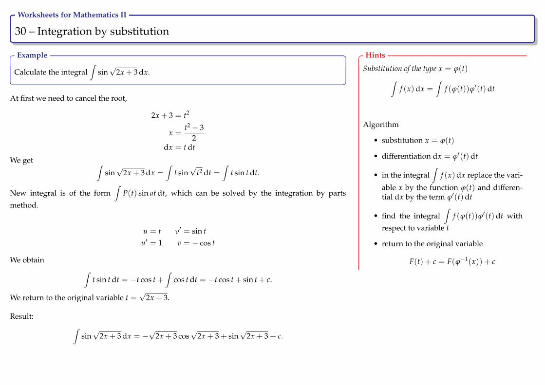
Example
Calculate the integral∫
sin√
2x + 3 dx.
At first we need to cancel the root,
2x + 3 = t2
x =t2 − 3
2dx = t dt
We get ∫sin√
2x + 3 dx =∫
t sin√
t2 dt =∫
t sin t dt.
New integral is of the form∫
P(t) sin at dt, which can be solved by the integration by parts
method.
u = t v′ = sin tu′ = 1 v = − cos t
We obtain ∫t sin t dt = −t cos t +
∫cos t dt = −t cos t + sin t + c.
We return to the original variable t =√
2x + 3.
Result: ∫sin√
2x + 3 dx = −√
2x + 3 cos√
2x + 3 + sin√
2x + 3 + c.
Hints
Substitution of the type x = ϕ(t)∫f (x)dx =
∫f (ϕ(t))ϕ′(t)dt
Algorithm
• substitution x = ϕ(t)
• differentiation dx = ϕ′(t)dt
• in the integral∫
f (x)dx replace the vari-
able x by the function ϕ(t) and differen-tial dx by the term ϕ′(t)dt
• find the integral∫
f (ϕ(t))ϕ′(t)dt with
respect to variable t
• return to the original variable
F(t) + c = F(ϕ−1(x)) + c

Worksheets for Mathematics II
31 – Integration by substitution Ry
Exercise
Solve:
a)∫ dx
(2 + x)√
1 + xb)∫ cot
√x√
xdx
Hints
Substitution of the type x = ϕ(t)∫f (x)dx =
∫f (ϕ(t))ϕ′(t)dt
Algorithm
• substitution x = ϕ(t)
• differentiation dx = ϕ′(t)dt
• in the integral∫
f (x)dx replace the vari-
able x by the function ϕ(t) and differen-tial dx by the term ϕ′(t)dt
• find the integral∫
f (ϕ(t))ϕ′(t)dt with
respect to variable t
• return to the original variable
F(t) + c = F(ϕ−1(x)) + c
Worksheets for Mathematics II
32 – Combination of both methods Ry
Exercise
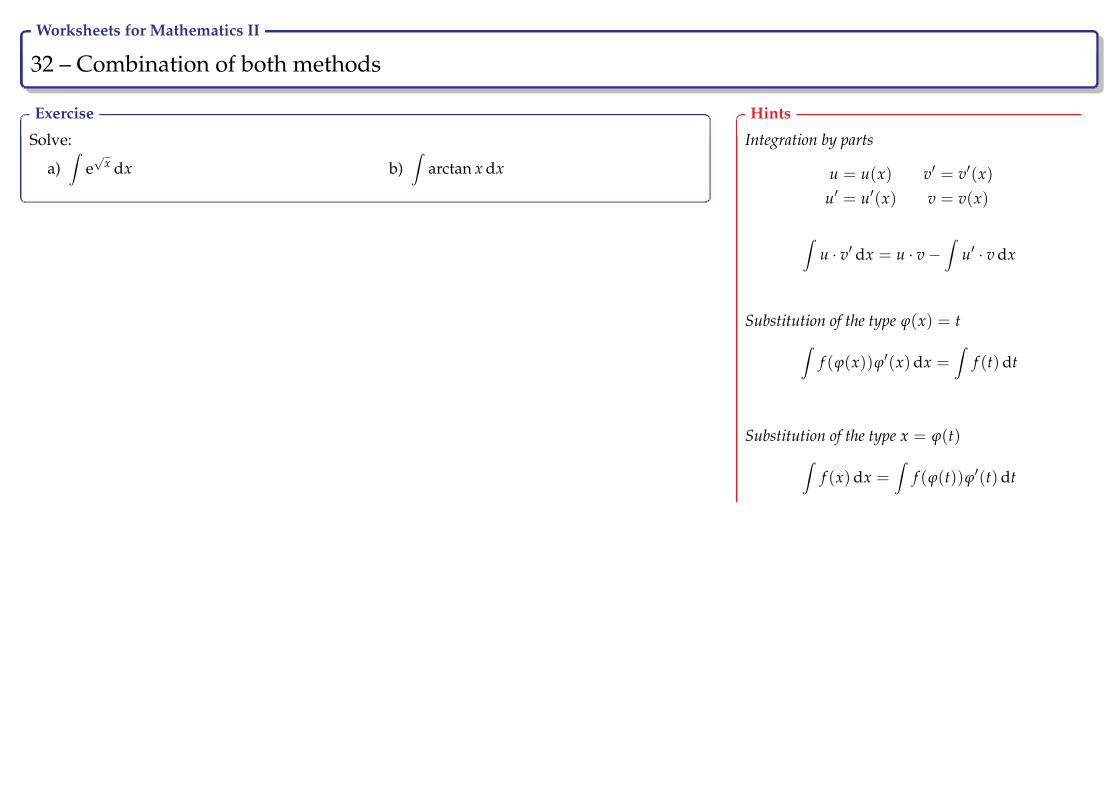
Solve:
a)∫
e√
x dx b)∫
arctan x dx
Hints
Integration by parts
u = u(x) v′ = v′(x)u′ = u′(x) v = v(x)
∫u · v′ dx = u · v−
∫u′ · v dx
Substitution of the type ϕ(x) = t∫f (ϕ(x))ϕ′(x)dx =
∫f (t)dt
Substitution of the type x = ϕ(t)∫f (x)dx =
∫f (ϕ(t))ϕ′(t)dt

Worksheets for Mathematics II
33 – Rational functions Ry
Every rational function of the form f (x) =P(x)Q(x)
, where P(x) and Q(x)
are polynomials of arbitrary degrees can be expressed as
P(x)Q(x)
= S(x) + R1(x) + ... + Rs(x),
where S(x) is a polynomial and R1(x), ..., Rs(x) are partial fractions.
Partial fractions are special rational functions. We specify two types:
A(x− α)k , k ∈N; α, A ∈ R,
where the polynomial x− α has real root α ∈ R and
Mx + N(x2 + px + q)k =
B(2x + p) + C(x2 + px + q)k , k ∈N; B, C, M, N, p, q ∈ R; p2− 4q < 0,
where the polynomial x2 + px + q has two complex conjugate roots.
Definition
Rational functionP(x)Q(x)
is called proper, if deg P(x) < deg Q(x), where
deg P(x) is the degree of the polynomial P(x).
Partial fraction decomposition of proper rational functions
• find the roots of the polynomial in denominator
• make decomposition
• multiply the equation by the polynomial in denominator
• find the coefficient of decomposition by either comparative methodor substitution method or combination of both methods.

Worksheets for Mathematics II
34 – Rational functions Ry
Example
Calculate the integral∫ x4 + 2
x− 1dx.
The polynomial in numerator has degree equal to four, the polynomial in denominator has degree equal to one.The function is not proper, we need to divide polynomials using standard Euclidean algorithm.
(x4 + 2) : (x− 1) = x3 + x2 + x + 1 +3
x− 1−(x4 − x3)
x3 + 2
−(x3 − x2)
x2 + 2
−(x2 − x)
x + 2−(x− 1)
3
We get ∫ x4 + 2x− 1
dx =∫ (
x3 + x2 + x + 1 +3
x− 1
)dx.
Result: ∫ x4 + 2x− 1
dx =x4
4+
x3
3+
x2
2+ x + 3 ln |x− 1|+ c.
Hints
Rational function
R(x) =Pn(x)Qm(x)
Proper rational function
R(x) =Pn(x)Qm(x)
, n < m
Improper rational function
R(x) =Pn(x)Qm(x)
, n ≥ m
every improper rational functionone can express as a sum of a poly-nomial and a proper rational func-tion by means of division of bothpolynomials
Worksheets for Mathematics II
35 – Rational functions Ry
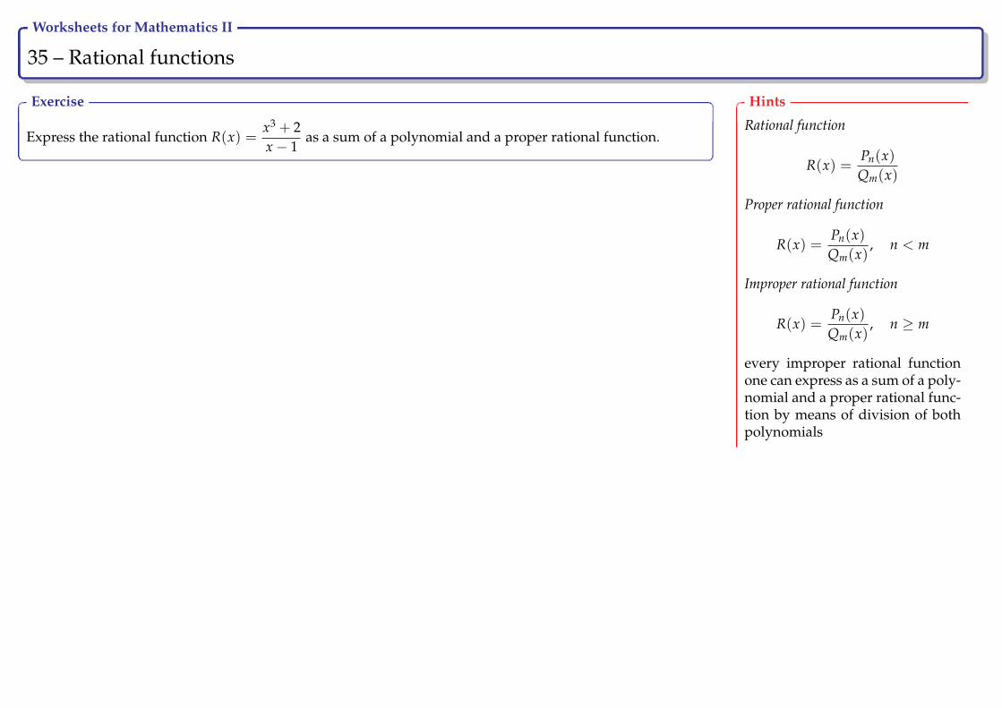
Exercise
Express the rational function R(x) =x3 + 2x− 1
as a sum of a polynomial and a proper rational function.
Hints
Rational function
R(x) =Pn(x)Qm(x)
Proper rational function
R(x) =Pn(x)Qm(x)
, n < m
Improper rational function
R(x) =Pn(x)Qm(x)
, n ≥ m
every improper rational functionone can express as a sum of a poly-nomial and a proper rational func-tion by means of division of bothpolynomials
Worksheets for Mathematics II
36 – Rational functions Ry
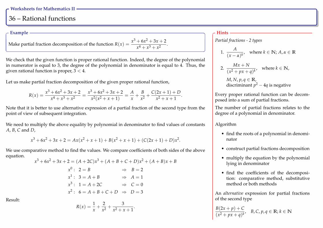
Example
Make partial fraction decomposition of the function R(x) =x3 + 6x2 + 3x + 2
x4 + x3 + x2 .
We check that the given function is proper rational function. Indeed, the degree of the polynomialin numerator is equal to 3, the degree of the polynomial in denominator is equal to 4. Thus, thegiven rational function is proper, 3 < 4.
Let us make partial fraction decomposition of the given proper rational function,
R(x) =x3 + 6x2 + 3x + 2
x4 + x3 + x2 =x3 + 6x2 + 3x + 2
x2(x2 + x + 1)=
Ax+
Bx2 +
C(2x + 1) + Dx2 + x + 1
.
Note that it is better to use alternative expression of a partial fraction of the second type from thepoint of view of subsequent integration.
We need to multiply the above equality by polynomial in denominator to find values of constantsA, B, C and D,
x3 + 6x2 + 3x + 2 = Ax(x2 + x + 1) + B(x2 + x + 1) + (C(2x + 1) + D)x2.
We use comparative method to find the values. We compare coefficients of both sides of the aboveequation.
x3 + 6x2 + 3x + 2 = (A + 2C)x3 + (A + B + C + D)x2 + (A + B)x + B
x0 : 2 = B ⇒ B = 2
x1 : 3 = A + B ⇒ A = 1
x3 : 1 = A + 2C ⇒ C = 0
x2 : 6 = A + B + C + D ⇒ D = 3
Result:R(x) =
1x+
2x2 +
3x2 + x + 1
.
Hints
Partial fractions - 2 types
1.A
(x− α)k , where k ∈N; A, α ∈ R
2.Mx + N
(x2 + px + q)k , where k ∈N,
M, N, p, q ∈ R,discriminant p2 − 4q is negative
Every proper rational function can be decom-posed into a sum of partial fractions.
The number of partial fractions relates to thedegree of a polynomial in denominator.
Algorithm
• find the roots of a polynomial in denomi-nator
• construct partial fractions decomposition
• multiply the equation by the polynomiallying in denominator
• find the coefficients of the decomposi-tion: comparative method, substitutivemethod or both methods
An alternative expression for partial fractionsof the second type
B(2x + p) + C(x2 + px + q)k , B, C, p, q ∈ R; k ∈N

Worksheets for Mathematics II
37 – Rational functions Ry
Exercise
Make partial fraction decomposition:
a) R(x) =2x− 1x3 − 4x
b) R(x) =1
x3 − 4x2 + 4x
Hints
Partial fractions - 2 types
1.A
(x− α)k , where k ∈N; A, α ∈ R
2.Mx + N
(x2 + px + q)k , where k ∈N,
M, N, p, q ∈ R,discriminant p2 − 4q is negative
Every proper rational function can be decom-posed into a sum of partial fractions.
The number of partial fractions relates to thedegree of a polynomial in denominator.
Algorithm
• find the roots of a polynomial in denomi-nator
• construct partial fractions decomposition
• multiply the equation by the polynomiallying in denominator
• find the coefficients of the decomposi-tion: comparative method, substitutivemethod or both methods
An alternative expression for partial fractionsof the second type
B(2x + p) + C(x2 + px + q)k , B, C, p, q ∈ R; k ∈N
Worksheets for Mathematics II
38 – Rational functions Ry
Exercise
Make partial fraction decomposition of the function R(x) =x
(x− 1)(x2 + 1).
Hints
Partial fractions - 2 types
1.A
(x− α)k , where k ∈N; A, α ∈ R
2.Mx + N
(x2 + px + q)k , where k ∈N,
M, N, p, q ∈ R,discriminant p2 − 4q is negative
Every proper rational function can be decom-posed into a sum of partial fractions.
The number of partial fractions relates to thedegree of a polynomial in denominator.
Algorithm
• find the roots of a polynomial in denomi-nator
• construct partial fractions decomposition
• multiply the equation by the polynomiallying in denominator
• find the coefficients of the decomposi-tion: comparative method, substitutivemethod or both methods
An alternative expression for partial fractionsof the second type
B(2x + p) + C(x2 + px + q)k , B, C, p, q ∈ R; k ∈N

Worksheets for Mathematics II
39 – Rational functions Ry
Integration of partial fractions with real roots in denominator
For simple roots: ∫ Ax− α
dx = A ln |x− α|+ c.
For k-fold roots (k > 1):∫ A(x− α)k dx =
A(1− k)(x− α)k−1 + c.
Integration of partial fractions with complex roots in denomina-tor
The integration of the fractionB(2x + p)
x2 + px + qleads to:
∫ B(2x + p)x2 + px + q
dx = B ln |x2 + px + q|+ c.
The integration of the fractionC
x2 + px + qmust be accompanied by con-
version of the triple x2 + px + q onto the perfect square:∫ Cx2 + px + q
dx = C∫ dx
(x + p/2)2 + r2 =Cr
arctanx + p/2
r+ c,
where
r =
√q− p2
4.

Worksheets for Mathematics II
40 – Rational functions Ry
Example
Calculate the integral∫ x + 2
x2 + x− 6dx.
The function is proper. We decompose denominator onto root factors,
x2 + x− 6 = (x− 2)(x + 3).
Partial fraction decomposition:
x + 2(x− 2)(x + 3)
=A
x− 2+
Bx + 3
.
Multiplying by (x− 2)(x + 3),
x + 2 = A(x + 3) + B(x− 2).
Substitution method:
x = 2 : 4 = 5A ⇒ A =45
x = −3 : −1 = −5B ⇒ B =15
We obtain two partial fractions of the first type,∫ x + 2x2 + x− 6
dx =45
∫ 1x− 2
dx +15
∫ 1x + 3
dx.
Result: ∫ x + 2x2 + x− 6
dx =45
ln |x− 2|+ 15
ln |x + 3|+ c.
Hints
Algorithm
• find the roots of polynomial in denomi-nator
• make partial fraction decomposition
• multiply the equation by polynomial indenominator
• find coefficients of decomposition: com-parative method, substitutive method orcombination of both methods
Integration of partial fractions∫ Ax− α
dx = A ln |x− α|+ c
∫ A(x− α)k dx =
A(1− k)(x− α)k−1 + c,
k ≥ 2
∫ B(2x + p)x2 + px + q
dx = B ln |x2 + px + q|+ c
∫ Cx2 + px + q
dx =Cr
arctanx + p/2
r+ c,
r =
√q− p2
4

Worksheets for Mathematics II
41 – Rational functions Ry
Example
Calculate the integral∫ −3x + 1
x2 + 4x + 4dx.
The function is proper. We decompose denominator onto root factors,
x2 + 4x + 4 = (x + 2)2.
Partial fraction decomposition:
−3x + 1(x + 2)2 =
Ax + 2
+B
(x + 2)2 .
Multiplying by (x + 2)2,
−3x + 1 = A(x + 2) + B.
Combination of both methods:
x = −2 : 7 = B
x0 : 1 = 2A + B ⇒ −6 = 2A ⇒ A = −3
We obtain partial fraction of the first and second type,∫ −3x + 1x2 + 4x + 4
dx = −3∫ 1
x + 2dx + 7
∫ 1(x + 2)2 dx.
Result: ∫ −3x + 1x2 + 4x + 4
dx = −3 ln |x + 2| − 7x + 2
+ c.
Hints
Algorithm
• find the roots of polynomial in denomi-nator
• make partial fraction decomposition
• multiply the equation by polynomial indenominator
• find coefficients of decomposition: com-parative method, substitutive method orcombination of both methods
Integration of partial fractions∫ Ax− α
dx = A ln |x− α|+ c
∫ A(x− α)k dx =
A(1− k)(x− α)k−1 + c,
k ≥ 2
∫ B(2x + p)x2 + px + q
dx = B ln |x2 + px + q|+ c
∫ Cx2 + px + q
dx =Cr
arctanx + p/2
r+ c,
r =
√q− p2
4

Worksheets for Mathematics II
42 – Rational functions Ry
Example
Calculate the integral∫ x
x2 + 3x + 4dx.
The function is proper. We decompose denominator onto root factors, but the polynomial has noreal roots.
Partial fraction decomposition:
xx2 + 3x + 4
=B(2x + 3)
x2 + 3x + 4+
Cx2 + 3x + 4
.
Multiplying by (x2 + 3x + 4),
x = B(2x + 3) + C.
Comparative method:
x1 : 1 = 2B ⇒ B =12
x0 : 0 = 3B + C ⇒ C = −32
We obtain partial fraction of the second type,∫ xx2 + 3x + 4
dx =12
∫ 2x + 3x2 + 3x + 4
dx− 32
∫ 1x2 + 3x + 4
dx.
We rewrite denominator of the second integrand as(
x +32
)2
+74
using completing the square
method.
Result:
∫ xx2 + 3x + 4
dx =ln(x2 + 3x + 4)
2− 3√
7arctan
2(x + 3
2
)√
7+ c.
Hints
Algorithm
• find the roots of polynomial in denomi-nator
• make partial fraction decomposition
• multiply the equation by polynomial indenominator
• find coefficients of decomposition: com-parative method, substitutive method orcombination of both methods
Integration of partial fractions∫ Ax− α
dx = A ln |x− α|+ c
∫ A(x− α)k dx =
A(1− k)(x− α)k−1 + c,
k ≥ 2
∫ B(2x + p)x2 + px + q
dx = B ln |x2 + px + q|+ c
∫ Cx2 + px + q
dx =Cr
arctanx + p/2
r+ c,
r =
√q− p2
4
Worksheets for Mathematics II
43 – Rational functions Ry
Exercise
Calculate the integrals
a)∫ x + 2
x3 − 2x2 − 8xdx b)
∫ 3x− 8(x− 4)(x− 2)2 dx
Hints
Integration of partial fractions
polynomial in denominator has real roots∫ Ax− α
dx = A ln |x− α|+ c
∫ A(x− α)k dx =
A(1− k)(x− α)k−1 + c,
k ≥ 2

Worksheets for Mathematics II
44 – Rational functions Ry
Exercise
Calculate the integrals
a)∫ 3x
(x2 + 1)(x2 + 4)dx b)
∫ 3x2 + 4x + 33(x2 + 9)(3− x)
dx
Hints
Integration of partial fractions
polynomial in denominator has complexroots∫ B(2x + p)
x2 + px + qdx = B ln |x2 + px + q|+ c
∫ Cx2 + px + q
dx =Cr
arctanx + p/2
r+ c,
r =
√q− p2
4
polynomial in denominator has a real root∫ Ax− α
dx = A ln |x− α|+ c
∫ A(x− α)k dx =
A(1− k)(x− α)k−1 + c,
k ≥ 2

Worksheets for Mathematics II
45 – Rational functions Ry
Exercise
Calculate the integrals
a)∫ x3
x3 + xdx b)
∫ 2x2 − 3x + 5x3(x + 1)
dx
Hints
Integration of partial fractions∫ Ax− α
dx = A ln |x− α|+ c
∫ A(x− α)k dx =
A(1− k)(x− α)k−1 + c,
k ≥ 2
∫ B(2x + p)x2 + px + q
dx = B ln |x2 + px + q|+ c
∫ Cx2 + px + q
dx =Cr
arctanx + p/2
r+ c,
r =
√q− p2
4
Worksheets for Mathematics II
46 – Trigonometric functions Ry
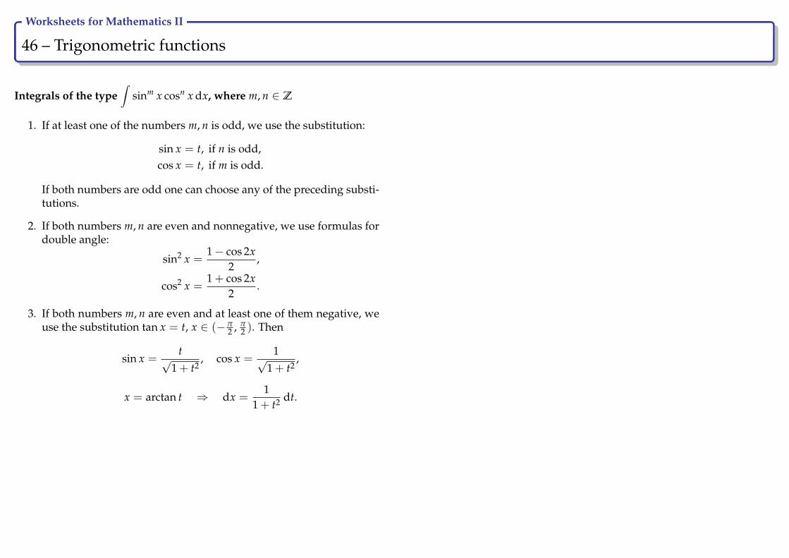
Integrals of the type∫
sinm x cosn x dx, where m, n ∈ Z
1. If at least one of the numbers m, n is odd, we use the substitution:
sin x = t, if n is odd,cos x = t, if m is odd.
If both numbers are odd one can choose any of the preceding substi-tutions.
2. If both numbers m, n are even and nonnegative, we use formulas fordouble angle:
sin2 x =1− cos 2x
2,
cos2 x =1 + cos 2x
2.
3. If both numbers m, n are even and at least one of them negative, weuse the substitution tan x = t, x ∈ (−π
2 , π2 ). Then
sin x =t√
1 + t2, cos x =
1√1 + t2
,
x = arctan t ⇒ dx =1
1 + t2 dt.
Worksheets for Mathematics II
47 – Trigonometric functions Ry
Example
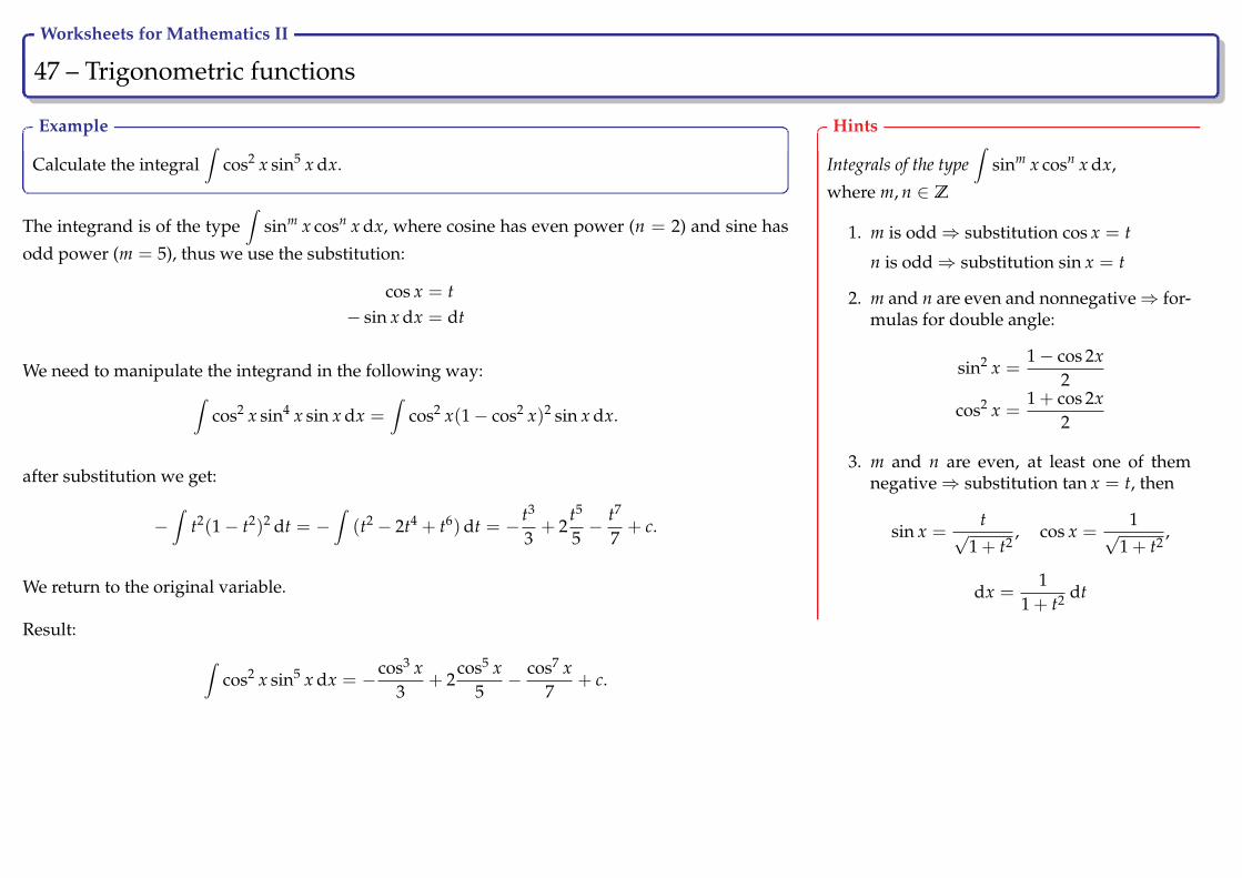
Calculate the integral∫
cos2 x sin5 x dx.
The integrand is of the type∫
sinm x cosn x dx, where cosine has even power (n = 2) and sine has
odd power (m = 5), thus we use the substitution:
cos x = t− sin x dx = dt
We need to manipulate the integrand in the following way:∫cos2 x sin4 x sin x dx =
∫cos2 x(1− cos2 x)2 sin x dx.
after substitution we get:
−∫
t2(1− t2)2 dt = −∫
(t2 − 2t4 + t6)dt = − t3
3+ 2
t5
5− t7
7+ c.
We return to the original variable.
Result: ∫cos2 x sin5 x dx = −cos3 x
3+ 2
cos5 x5− cos7 x
7+ c.
Hints
Integrals of the type∫
sinm x cosn x dx,
where m, n ∈ Z
1. m is odd⇒ substitution cos x = t
n is odd⇒ substitution sin x = t
2. m and n are even and nonnegative⇒ for-mulas for double angle:
sin2 x =1− cos 2x
2
cos2 x =1 + cos 2x
2
3. m and n are even, at least one of themnegative⇒ substitution tan x = t, then
sin x =t√
1 + t2, cos x =
1√1 + t2
,
dx =1
1 + t2 dt

Worksheets for Mathematics II
48 – Trigonometric functions Ry
Example
Calculate the integral∫
sin2 x cos x dx.
Integrand is of the type∫
sinm x cosn x dx, where cosine has odd power and sine has even power,
then we use the substitution,
sin x = tcos x dx = dt
After substitution we get: ∫t2 dt =
t3
3+ c.
We return to the original variable.
Result: ∫sin2 x cos x dx =
sin3 x3
+ c.
Hints
Integrals of the type∫
sinm x cosn x dx,
where m, n ∈ Z
1. m is odd⇒ substitution cos x = t
n is odd⇒ substitution sin x = t
2. m and n are even and nonnegative⇒ for-mulas for double angle:
sin2 x =1− cos 2x
2
cos2 x =1 + cos 2x
2
3. m and n are even, at least one of themnegative⇒ substitution tan x = t, then
sin x =t√
1 + t2, cos x =
1√1 + t2
,
dx =1
1 + t2 dt
Worksheets for Mathematics II
49 – Trigonometric functions Ry
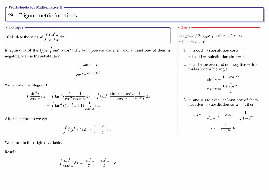
Example
Calculate the integral∫ sin4 x
cos8 xdx.
Integrand is of the type∫
sinm x cosn x dx, both powers are even and at least one of them is
negative, we use the substitution,
tan x = t1
cos2 xdx = dt
We rewrite the integrand:∫ sin4 xcos8 x
dx =∫
tan4 x1
cos2 x1
cos2 xdx =
∫tan4 x
sin2 x + cos2 xcos2 x
1cos2 x
dx
=∫
tan4 x(tan2 x + 1)1
cos2 xdx.
After substitution we get ∫t4(t2 + 1)dt =
t7
7+
t5
5+ c.
We return to the original variable.
Result: ∫ sin4 xcos8 x
dx =tan7 x
7+
tan5 x5
+ c.
Hints
Integrals of the type∫
sinm x cosn x dx,
where m, n ∈ Z
1. m is odd⇒ substitution cos x = t
n is odd⇒ substitution sin x = t
2. m and n are even and nonnegative⇒ for-mulas for double angle:
sin2 x =1− cos 2x
2
cos2 x =1 + cos 2x
2
3. m and n are even, at least one of themnegative⇒ substitution tan x = t, then
sin x =t√
1 + t2, cos x =
1√1 + t2
,
dx =1
1 + t2 dt

Worksheets for Mathematics II
50 – Trigonometric functions Ry
Example
Calculate the integral∫
sin2 x cos2 x dx.
Integrand is of the type∫
sinm x cosn x dx, both powers are even and nonnegative, then we use the
formulas for double angle:∫sin2 x cos2 x dx =
∫ (1− cos 2x2
)(1 + cos 2x
2
)dx =
14
∫(1− cos2 2x)dx.
Again we use the same formula for double angle:
14
∫(1− cos2 2x)dx =
14
∫ (1− 1 + cos 4x
2
)dx =
14
∫ (12− cos 4x
2
)dx.
Result: ∫sin2 x cos2 x dx =
x8− sin 4x
32+ c.
Hints
Integrals of the type∫
sinm x cosn x dx,
where m, n ∈ Z
1. m is odd⇒ substitution cos x = t
n is odd⇒ substitution sin x = t
2. m and n are even and nonnegative⇒ for-mulas for double angle:
sin2 x =1− cos 2x
2
cos2 x =1 + cos 2x
2
3. m and n are even, at least one of themnegative⇒ substitution tan x = t, then
sin x =t√
1 + t2, cos x =
1√1 + t2
,
dx =1
1 + t2 dt
Worksheets for Mathematics II
51 – Trigonometric functions Ry
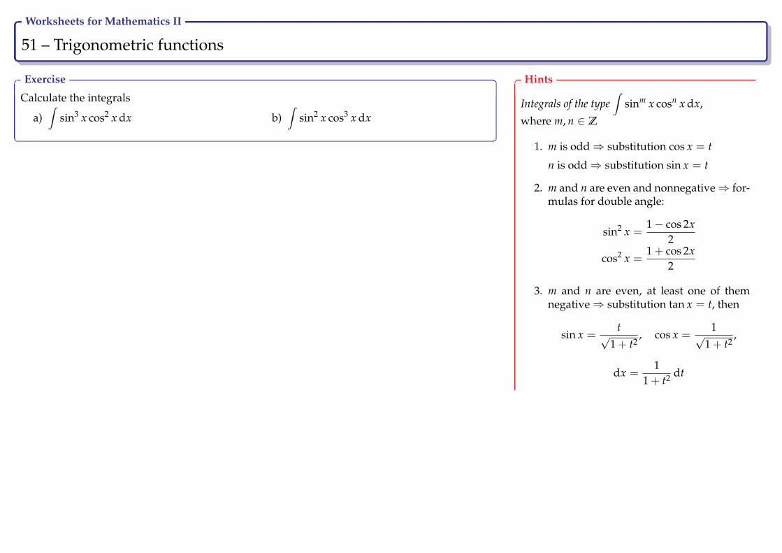
Exercise
Calculate the integrals
a)∫
sin3 x cos2 x dx b)∫
sin2 x cos3 x dx
Hints
Integrals of the type∫
sinm x cosn x dx,
where m, n ∈ Z
1. m is odd⇒ substitution cos x = t
n is odd⇒ substitution sin x = t
2. m and n are even and nonnegative⇒ for-mulas for double angle:
sin2 x =1− cos 2x
2
cos2 x =1 + cos 2x
2
3. m and n are even, at least one of themnegative⇒ substitution tan x = t, then
sin x =t√
1 + t2, cos x =
1√1 + t2
,
dx =1
1 + t2 dt

Worksheets for Mathematics II
52 – Trigonometric functions Ry
Exercise
Calculate the integrals
a)∫ sin2 x
cos6 xdx b)
∫cos4 x dx
Hints
Integrals of the type∫
sinm x cosn x dx,
where m, n ∈ Z
1. m is odd⇒ substitution cos x = t
n is odd⇒ substitution sin x = t
2. m and n are even and nonnegative⇒ for-mulas for double angle:
sin2 x =1− cos 2x
2
cos2 x =1 + cos 2x
2
3. m and n are even, at least one of themnegative⇒ substitution tan x = t, then
sin x =t√
1 + t2, cos x =
1√1 + t2
,
dx =1
1 + t2 dt
Worksheets for Mathematics II
53 – Trigonometric functions, universal substitution Ry
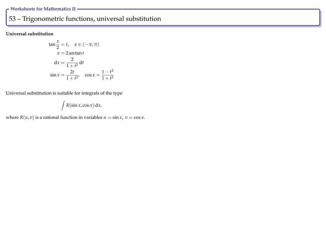
Universal substitution
tanx2= t, x ∈ (−π, π)
x = 2 arctan t
dx =2
1 + t2 dt
sin x =2t
1 + t2 , cos x =1− t2
1 + t2
Universal substitution is suitable for integrals of the type∫R(sin x, cos x)dx,
where R(u, v) is a rational function in variables u = sin x, v = cos x.

Worksheets for Mathematics II
54 – Trigonometric functions, universal substitution Ry
Example
Calculate the integral∫ −3
2 + cos xdx.
Integrand is a rational function containing trigonometric functions, we use universal substitution:∫ −32 + cos x
dx =∫ −3
2 + 1−t2
1+t2
21 + t2 dt =
∫ −63 + t2 dt.
Using general formula ∫ 1a2 + x2 dx =
1a
arctanxa+ c
we get: ∫ −63 + t2 dt =
−6√3
arctant√3+ c.
Result:
∫ −32 + cos x
dx = −2√
3 arctan
√3 tan x
23
+ c.
Hints
Integrals of the type∫R(sin x, cos x)dx,
where R(u, v) represent a rationalfunction with variables u = sin xand v = cos x
Universal substitution
tanx2= t, x ∈ (−π, π)
sin x =2t
1 + t2
cos x =1− t2
1 + t2
x = 2 arctan t
dx =2
1 + t2 dt
Worksheets for Mathematics II
55 – Trigonometric functions, universal substitution Ry
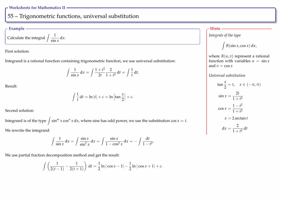
Example
Calculate the integral∫ 1
sin xdx.
First solution:
Integrand is a rational function containing trigonometric function, we use universal substitution:∫ 1sin x
dx =∫ 1 + t2
2t2
1 + t2 dt =∫ 1
tdt.
Result: ∫ 1t
dt = ln |t|+ c = ln∣∣∣tan
x2
∣∣∣+ c.
Second solution:
Integrand is of the type∫
sinm x cosn x dx, where sine has odd power, we use the substitution cos x = t.
We rewrite the integrand: ∫ 1sin x
dx =∫ sin x
sin2 xdx =
∫ sin x1− cos2 x
dx = −∫ dt
1− t2 .
We use partial fraction decomposition method and get the result:∫ ( 12(t− 1)
− 12(t + 1)
)dt =
12
ln | cos x− 1| − 12
ln | cos x + 1|+ c.
Hints
Integrals of the type∫R(sin x, cos x)dx,
where R(u, v) represent a rationalfunction with variables u = sin xand v = cos x
Universal substitution
tanx2= t, x ∈ (−π, π)
sin x =2t
1 + t2
cos x =1− t2
1 + t2
x = 2 arctan t
dx =2
1 + t2 dt

Worksheets for Mathematics II
56 – Trigonometric functions, universal substitution Ry
Exercise
Calculate the integrals
a)∫ 1
2 sin x + 1dx b)
∫ 11 + cos x + sin x
dx
Hints
Integrals of the type∫R(sin x, cos x)dx,
where R(u, v) represent a rationalfunction with variables u = sin xand v = cos x
Universal substitution
tanx2= t, x ∈ (−π, π)
sin x =2t
1 + t2
cos x =1− t2
1 + t2
x = 2 arctan t
dx =2
1 + t2 dt
Worksheets for Mathematics II
57 – Irrational functions Ry
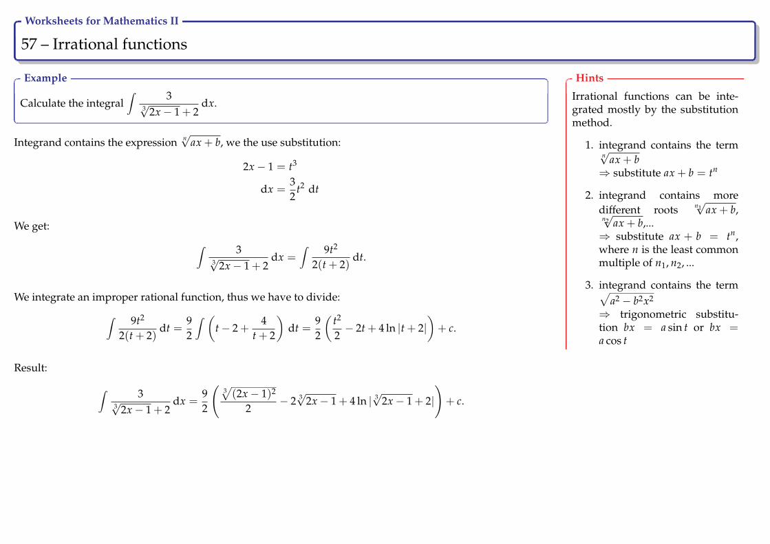
Example
Calculate the integral∫ 3
3√
2x− 1 + 2dx.
Integrand contains the expression n√
ax + b, we the use substitution:
2x− 1 = t3
dx =32
t2 dt
We get: ∫ 33√
2x− 1 + 2dx =
∫ 9t2
2(t + 2)dt.
We integrate an improper rational function, thus we have to divide:∫ 9t2
2(t + 2)dt =
92
∫ (t− 2 +
4t + 2
)dt =
92
(t2
2− 2t + 4 ln |t + 2|
)+ c.
Result:
∫ 33√
2x− 1 + 2dx =
92
(3√(2x− 1)2
2− 2 3√
2x− 1 + 4 ln | 3√
2x− 1 + 2|)+ c.
Hints
Irrational functions can be inte-grated mostly by the substitutionmethod.
1. integrand contains the termn√
ax + b⇒ substitute ax + b = tn
2. integrand contains moredifferent roots n1
√ax + b,
n2√
ax + b,...⇒ substitute ax + b = tn,where n is the least commonmultiple of n1, n2, ...
3. integrand contains the term√a2 − b2x2
⇒ trigonometric substitu-tion bx = a sin t or bx =a cos t

Worksheets for Mathematics II
58 – Irrational functions Ry
Example
Calculate the integral∫ √
x4√
x + 2dx.
Integrand contains more different roots, we use the substitution:
x = t4
dx = 4t3 dt
We get: ∫ √x
4√
x + 2dx = 4
∫ t2
t + 2t3 dt.
We obtained an improper rational function, we have to divide:
4∫ (
t4 − 2t3 + 4t2 − 8t + 16− 32t + 2
)dt = 4
(t5
5− t4
2+
4t3
3− 4t2 + 16t− 32 ln |t + 2|
)+ c.
Result:
∫ √x
4√
x + 2dx = 4
(4√
x5
5− x
2+
4 4√
x3
3− 4√
x + 16 4√
x− 32 ln | 4√
x + 2|)+ c.
Hints
Irrational functions can be inte-grated mostly by the substitutionmethod.
1. integrand contains the termn√
ax + b⇒ substitute ax + b = tn
2. integrand contains moredifferent roots n1
√ax + b,
n2√
ax + b,...⇒ substitute ax + b = tn,where n is the least commonmultiple of n1, n2, ...
3. integrand contains the term√a2 − b2x2
⇒ trigonometric substitu-tion bx = a sin t or bx =a cos t

Worksheets for Mathematics II
59 – Irrational functions Ry
Example
Calculate the integral∫ √
9− 16x2 dx.
Integrand contains√
a2 − b2x2, we use the substitution:
4x = 3 sin t4dx = 3 cos t dt
We get: ∫ √9− 16x2 dx =
34
∫ √9− 9 sin2 t cos t dt =
34
∫ √9(1− sin2 t) cos t dt =
34
∫3 cos2 t dt.
We need to use the formula for double angle:
94
∫cos2 t dt =
98
∫(1 + cos 2t)dt =
98
(t +
sin 2t2
)+ c =
98
(t +
2 sin t cos t2
)+ c
=98
(t + sin t
√(1− sin2 t)
)+ c.
Result:
∫ √9− 16x2 dx =
98
(arcsin
4x3
+4x3
√1− 16x2
9
)+ c =
98
arcsin4x3
+x2
√9− 16x2 + c.
Hints
Irrational functions can be inte-grated mostly by the substitutionmethod.
1. integrand contains the termn√
ax + b⇒ substitute ax + b = tn
2. integrand contains moredifferent roots n1
√ax + b,
n2√
ax + b,...⇒ substitute ax + b = tn,where n is the least commonmultiple of n1, n2, ...
3. integrand contains the term√a2 − b2x2
⇒ trigonometric substitu-tion bx = a sin t or bx =a cos t

Worksheets for Mathematics II
60 – Irrational functions Ry
Exercise
Calculate the integrals
a)∫ 1 + 5x
3√
x + 5dx b)
∫ 3√
xx +√
xdx
Hints
Irrational functions can be inte-grated mostly by the substitutionmethod.
1. integrand contains the termn√
ax + b⇒ substitute ax + b = tn
2. integrand contains moredifferent roots n1
√ax + b,
n2√
ax + b,...⇒ substitute ax + b = tn,where n is the least commonmultiple of n1, n2, ...
3. integrand contains the term√a2 − b2x2
⇒ trigonometric substitu-tion bx = a sin t or bx =a cos t

Worksheets for Mathematics II
61 – Irrational functions Ry
Exercise
Calculate the integrals
a)∫ dx√
(9− x2)3b)∫ √
4− x2 dx
Hints
Irrational functions can be inte-grated mostly by the substitutionmethod.
1. integrand contains the termn√
ax + b⇒ substitute ax + b = tn
2. integrand contains moredifferent roots n1
√ax + b,
n2√
ax + b,...⇒ substitute ax + b = tn,where n is the least commonmultiple of n1, n2, ...
3. integrand contains the term√a2 − b2x2
⇒ trigonometric substitu-tion bx = a sin t or bx =a cos t
Worksheets for Mathematics II
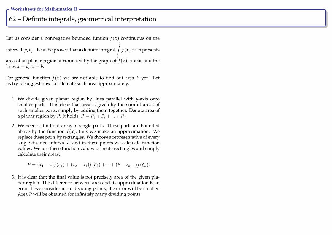
62 – Definite integrals, geometrical interpretation Ry
Let us consider a nonnegative bounded funtion f (x) continuous on the
interval [a, b]. It can be proved that a definite integralb∫
a
f (x)dx represents
area of an planar region surrounded by the graph of f (x), x-axis and thelines x = a, x = b.
For general function f (x) we are not able to find out area P yet. Letus try to suggest how to calculate such area approximately:
1. We divide given planar region by lines parallel with y-axis ontosmaller parts. It is clear that area is given by the sum of areas ofsuch smaller parts, simply by adding them together. Denote area ofa planar region by P. It holds: P = P1 + P2 + ... + Pn.
2. We need to find out areas of single parts. These parts are boundedabove by the function f (x), thus we make an approximation. Wereplace these parts by rectangles. We choose a representative of everysingle divided interval ξi and in these points we calculate functionvalues. We use these function values to create rectangles and simplycalculate their areas:
P .= (x1 − a) f (ξ1) + (x2 − x1) f (ξ2) + ... + (b− xn−1) f (ξn).
3. It is clear that the final value is not precisely area of the given pla-nar region. The difference between area and its approximation is anerror. If we consider more dividing points, the error will be smaller.Area P will be obtained for infinitely many dividing points.
Worksheets for Mathematics II
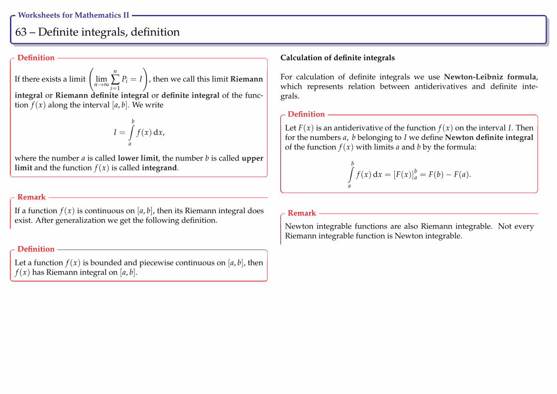
63 – Definite integrals, definition Ry
Definition
If there exists a limit
(lim
n→∞
n
∑i=1
Pi = I
), then we call this limit Riemann
integral or Riemann definite integral or definite integral of the func-tion f (x) along the interval [a, b]. We write
I =b∫
a
f (x)dx,
where the number a is called lower limit, the number b is called upperlimit and the function f (x) is called integrand.
Remark
If a function f (x) is continuous on [a, b], then its Riemann integral doesexist. After generalization we get the following definition.
Definition
Let a function f (x) is bounded and piecewise continuous on [a, b], thenf (x) has Riemann integral on [a, b].
Calculation of definite integrals
For calculation of definite integrals we use Newton-Leibniz formula,which represents relation between antiderivatives and definite inte-grals.
Definition
Let F(x) is an antiderivative of the function f (x) on the interval I. Thenfor the numbers a, b belonging to I we define Newton definite integralof the function f (x) with limits a and b by the formula:
b∫a
f (x)dx = [F(x)]ba = F(b)− F(a).
Remark
Newton integrable functions are also Riemann integrable. Not everyRiemann integrable function is Newton integrable.

Worksheets for Mathematics II
64 – Definite integrals, properties Ry
Theorem
Let functions f (x) and g(x) be integrable on [a, b], then their sum, dif-ference and constant factor are integrable on this interval and holds:
b∫a
( f (x)± g(x))dx =
b∫a
f (x)dx±b∫
a
g(x)dx,
b∫a
k · f (x)dx = kb∫
a
f (x)dx, c ∈ R.
Additional properties:
Theorem
Let f (x) and g(x) be integrable on [a, b], then it holds:
a∫a
f (x)dx = 0,
a∫b
f (x)dx = −b∫
a
f (x)dx,
∣∣∣∣∣∣b∫
a
f (x)dx
∣∣∣∣∣∣ ≤b∫
a
| f (x)dx|,
if f (x) ≤ g(x) ∀x ∈ [a, b], thenb∫
a
f (x)dx ≤b∫
a
g(x)dx.
The following property is suitable especially in the cases when integranddoes not have a uniform analytic formula on the interval [a, b].
Theorem
Let f (x) be integrable on [a, b] and let c be an arbitrary real numbera < c < b. Then f (x) is integrable on the intervals [a, c] and [c, b] andholds:
b∫a
f (x)dx =
c∫a
f (x)dx +
b∫c
f (x)dx.
Even and odd functions
If a function f (x) is even on the interval [−a, a], then
a∫−a
f (x)dx = 2a∫
0
f (x)dx.
If a function f (x) is odd on the interval [−a, a], then
a∫−a
f (x)dx = 0.

Worksheets for Mathematics II
65 – Definite integrals, calculation Ry
Example
Calculate the integralπ∫
0
((4− x)2 + cos 2x)dx.
Using properties one can represent the integral as a sum of four integrals:
π∫0
(16− 8x + x2 + cos 2x)dx = 16π∫
0
dx− 8π∫
0
x dx +
π∫0
x2 dx +
π∫0
cos 2x dx.
All integrals are elementary, thus it is easy to find appropriate antiderivatives. Finally, Newton-Leibniz formula is applied:
16π∫
0
dx− 8π∫
0
x dx +
π∫0
x2 dx +
π∫0
cos 2x dx = 16[x]π0 − 4[x2]π0 +
[x3
3
]π
0+
[sin 2x
2
]π
0
= 16(π − 0)− 4(π2 − 0) +(
π3
3− 0)+ (0− 0) = 16π − 4π2 +
π3
3.
Result:
π∫0
((4− x)2 + cos 2x)dx = 16π − 4π2 +π3
3.
Hints
Newton-Leibniz formula
b∫a
f (x)dx = [F(x)]ba = F(b)− F(a)
Properties
f = f (x), g = g(x), k ∈ R
b∫a
( f + g)dx =
b∫a
f dx +
b∫a
g dx
b∫a
k · f dx = kb∫
a
f dx

Worksheets for Mathematics II
66 – Definite integrals, calculation Ry
Exercise
Solve:
a)2∫
1
(3x2 + 1)dx b)1∫
0
(3− x2)2 dx c)1∫−1
x2
1 + x2 dx
Hints
Newton-Leibniz formula
b∫a
f (x)dx = [F(x)]ba = F(b)− F(a)
Properties
f = f (x), g = g(x), k ∈ R
b∫a
( f + g)dx =
b∫a
f dx +
b∫a
g dx
b∫a
k · f dx = kb∫
a
f dx

Worksheets for Mathematics II
67 – Definite integral, properties Ry
Example
Calculate the integrals:
π4∫
−π4
tan x dx,1∫−1
x4
2dx.
First integral,
π4∫
−π4
tan x dx:
The function tangent is odd on the interval [−π4 , π
4 ], thus the integral is null.
Verify:
π4∫
−π4
tan x dx =
π4∫
−π4
sin xcos x
dx = −[ln | cos x|]π4−π
4= −
(ln
√2
2− ln
√2
2
)= 0.
Second integral,1∫−1
x4
2dx:
The function x4
2 is even on the interval [−1, 1], thus:
1∫−1
x4
2dx = 2
1∫0
x4
2dx =
15[x5]10 =
15(1− 0) =
15
.
Hints
Even and odd functions
• even function:a∫−a
f (x)dx = 2a∫
0
f (x)dx
• odd function:a∫−a
f (x)dx = 0
0
y = tan x
x = π2x = −π
2
−3 −2 −1 1 2 3
−3
−2
−1
1
2
x = −π4 x = π
4
0
y =x4
2
x = −1 x = 1−3 −2 −1 1 2 3
1
2
3
Worksheets for Mathematics II
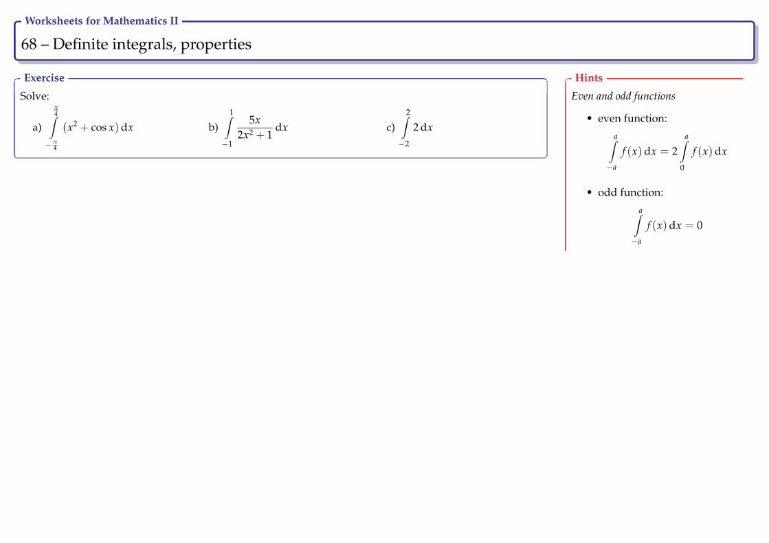
68 – Definite integrals, properties Ry
Exercise
Solve:
a)
π4∫
−π4
(x2 + cos x)dx b)1∫−1
5x2x2 + 1
dx c)2∫−2
2 dx
Hints
Even and odd functions
• even function:
a∫−a
f (x)dx = 2a∫
0
f (x)dx
• odd function:
a∫−a
f (x)dx = 0

Worksheets for Mathematics II
69 – Integration by parts and substitution Ry
Integration by parts for definite integrals
Theorem
Let functions u(x) and v(x) have derivatives integrable on [a, b], a < b,then it holds
b∫a
u(x) · v′(x)dx = [u(x) · v(x)]ba −b∫
a
u′(x) · v(x)dx.
Remark
We use this method in the same way as in the case of indefinite integrals.There is an advantage, we can evaluate antiderivatives due to ongoingcalculation. The calculation gets shorter and smoother.
Substitution for definite integrals
Theorem
If a function f (x) is integrable on [a, b] and strictly monotonic functionx = ϕ(t) has continuous derivative ϕ′(t) on the interval [α, β], whereasϕ(α) = a and ϕ(β) = b, then it holds:
b∫a
f (x)dx =
β∫α
f (ϕ(t))ϕ′(t)dt.
Remark
The calculation procedure and the notation are similar as in the caseof indefinite integrals, only new limits must be determined. There isan advantage, we do not need to return to the original variable aftersubstitution.

Worksheets for Mathematics II
70 – Integration by parts method for definite integrals Ry
Example
Calculate the integral2∫
1
ln x2 dx.
Integrand is a composite function, let us try the integration by parts method:
u = ln x2 v′ = 1
u′ =2x
v = x
After the application:
2∫1
ln x2 dx = [x ln x2]21 −2∫
1
2 dx = 2 ln 4− ln 1− 2[x]21 = 2 ln 4− 2(2− 1).
Result:
2∫1
ln x2 dx = 2(ln 4− 1).
Hints
Integration by parts method
u = u(x) v′ = v′(x)u′ = u′(x) v = v(x)
b∫a
(u · v′)dx = [u · v]ba −b∫
a
(u′ · v)dx

Worksheets for Mathematics II
71 – Integration by parts method for definite integrals Ry
Exercise
Solve:
a)1∫
0
(x + 2)ex dx b)
√3∫
0
x arctan x dx
Hints
Integration by parts method
u = u(x) v′ = v′(x)u′ = u′(x) v = v(x)
b∫a
(u · v′)dx = [u · v]ba −b∫
a
(u′ · v)dx
Worksheets for Mathematics II
72 – Substitution method for definite integrals Ry
Example
Calculate the integralπ∫
0
x cos x2 dx.
Integrand is in the form of a multiple of two functions, where derivative of interior function is directly theother function of the multiple (it differs up to a constant), we use the substitution:
x2 = t2x dx = dt
New limits for t:
lower limit : 0 7→ 02 = 0
upper limit : π 7→ π2
After the application:
π∫0
x cos x2 dx =12
π2∫0
cos t dt =12[sin t]π
2
0 =12(sin π2 − 0).
Result:
π∫0
x cos x2 dx =sin π2
2.
Hints
Substitution method
β∫α
f (ϕ(x))ϕ′(x)dx =
ϕ(β)∫ϕ(α)
f (t)dt
After substitution the new limitsmust be determined.

Worksheets for Mathematics II
73 – Substitution method for definite integrals Ry
Example
Calculate the integral8∫
3
x√x + 1 + 1
dx.
It is integral with the root. We use the substitution:
x + 1 = t2
dx = 2t dt
New limits for t:
lower limit : 3 7→√
3 + 1 = 2
upper limit : 8 7→√
8 + 1 = 3
After the application:
8∫3
x√x + 1− 1
dx =
3∫2
2tt2 − 1t + 1
dt = 23∫
2
t(t− 1)dt = 2[
t3
3− t2
2
]3
2= 2
(273− 9
2−(
83− 4
2
)).
Result:
8∫3
x√x + 1− 1
dx =233
.
Hints
Substitution of the type x = ϕ(t)
β∫α
f (x)dx =
ϕ−1(β)∫ϕ−1(α)
f (ϕ(t))ϕ′(t)dt
After substitution the new limitsmust be determined.

Worksheets for Mathematics II
74 – Substitution method for definite integrals Ry
Exercise
Solve:
a)e∫
1
1 + ln xx
dx b)
π2∫
0
sin x√
cos x dx
Hints
Substitution method
β∫α
f (ϕ(x))ϕ′(x)dx =
ϕ(β)∫ϕ(α)
f (t)dt
After substitution the new limitsmust be determined.
Worksheets for Mathematics II
75 – Combination of both methods Ry
Exercise
Solve:
a)3∫
1
x ln(x2 + 2)dx b)
12∫
0
arcsin 2x dx
Hints
Substitution method
β∫α
f (ϕ(x))ϕ′(x)dx =
ϕ(β)∫ϕ(α)
f (t)dt
After substitution the new limits must bedetermined.
Integration by parts method
u = u(x) v′ = v′(x)u′ = u′(x) v = v(x)
b∫a
(u · v′)dx = [u · v]ba −b∫
a
(u′ · v)dx
Worksheets for Mathematics II
76 – Definite integrals, rational functions Ry
Example
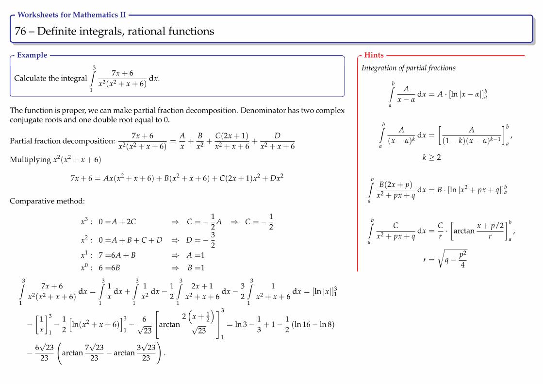
Calculate the integral3∫
1
7x + 6x2(x2 + x + 6)
dx.
The function is proper, we can make partial fraction decomposition. Denominator has two complexconjugate roots and one double root equal to 0.
Partial fraction decomposition:7x + 6
x2(x2 + x + 6)=
Ax+
Bx2 +
C(2x + 1)x2 + x + 6
+D
x2 + x + 6
Multiplying x2(x2 + x + 6)
7x + 6 = Ax(x2 + x + 6) + B(x2 + x + 6) + C(2x + 1)x2 + Dx2
Comparative method:
x3 : 0 =A + 2C ⇒ C =− 12
A ⇒ C =− 12
x2 : 0 =A + B + C + D ⇒ D =− 32
x1 : 7 =6A + B ⇒ A =1
x0 : 6 =6B ⇒ B =1
3∫1
7x + 6x2(x2 + x + 6)
dx =
3∫1
1x
dx +
3∫1
1x2 dx− 1
2
3∫1
2x + 1x2 + x + 6
dx− 32
3∫1
1x2 + x + 6
dx = [ln |x|]31
−[
1x
]3
1− 1
2
[ln(x2 + x + 6)
]3
1− 6√
23
arctan2(
x + 12
)√
23
3
1
= ln 3− 13+ 1− 1
2(ln 16− ln 8)
− 6√
2323
(arctan
7√
2323− arctan
3√
2323
).
Hints
Integration of partial fractions
b∫a
Ax− α
dx = A · [ln |x− α|]ba
b∫a
A(x− α)k dx =
[A
(1− k)(x− α)k−1
]b
a,
k ≥ 2
b∫a
B(2x + p)x2 + px + q
dx = B · [ln |x2 + px + q|]ba
b∫a
Cx2 + px + q
dx =Cr·[
arctanx + p/2
r
]b
a,
r =
√q− p2
4

Worksheets for Mathematics II
77 – Definite integrals, rational functions Ry
Exercise
Solve:
a)
√3∫
1
x + 2x(x2 + 1)
dx b)2∫
1
x− 1x3(x + 1)
dx
Hints
Integration of partial fractions
b∫a
Ax− α
dx = A · [ln |x− α|]ba
b∫a
A(x− α)k dx =
[A
(1− k)(x− α)k−1
]b
a,
k ≥ 2
b∫a
B(2x + p)x2 + px + q
dx = B · [ln |x2 + px + q|]ba
b∫a
Cx2 + px + q
dx =Cr·[
arctanx + p/2
r
]b
a,
r =
√q− p2
4
Worksheets for Mathematics II
78 – Improper integral of the first kind Ry
Definition
Let a function f (x) be continuous on the interval [a, ∞), then the integral
∞∫a
f (x)dx = limc→∞
∫ c
af (x)dx = L
is called improper integral of the first kind. If L ∈ R, we say thatthe improper integral is convergent. In the opposite case (L = ∞ orL = −∞) we say that the improper integral is divergent.
Remark
• Quite analogously we define improper integral of the first kind onthe interval (−∞, a].
• We integrate a bounded function on an unbounded interval.
• If a function f (x) is continuous on the interval (−∞, ∞) and bothimproper integrals are convergent for arbitrary number a,
L1 =
a∫−∞
f (x)dx, L2 =
∞∫a
f (x)dx,
then∞∫−∞
f (x)dx = L1 + L2.
Worksheets for Mathematics II
79 – Improper integral of the first kind Ry
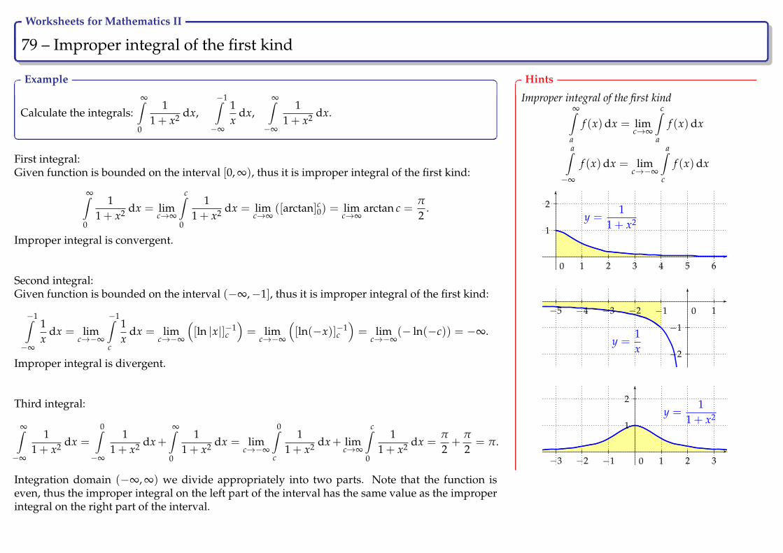
Example
Calculate the integrals:∞∫
0
11 + x2 dx,
−1∫−∞
1x
dx,∞∫−∞
11 + x2 dx.
First integral:Given function is bounded on the interval [0, ∞), thus it is improper integral of the first kind:
∞∫0
11 + x2 dx = lim
c→∞
c∫0
11 + x2 dx = lim
c→∞([arctan]c0) = lim
c→∞arctan c =
π
2.
Improper integral is convergent.
Second integral:Given function is bounded on the interval (−∞,−1], thus it is improper integral of the first kind:
−1∫−∞
1x
dx = limc→−∞
−1∫c
1x
dx = limc→−∞
([ln |x|]−1
c
)= lim
c→−∞
([ln(−x)]−1
c
)= lim
c→−∞(− ln(−c)) = −∞.
Improper integral is divergent.
Third integral:
∞∫−∞
11 + x2 dx =
0∫−∞
11 + x2 dx+
∞∫0
11 + x2 dx = lim
c→−∞
0∫c
11 + x2 dx+ lim
c→∞
c∫0
11 + x2 dx =
π
2+
π
2= π.
Integration domain (−∞, ∞) we divide appropriately into two parts. Note that the function iseven, thus the improper integral on the left part of the interval has the same value as the improperintegral on the right part of the interval.
Hints
Improper integral of the first kind∞∫
a
f (x)dx = limc→∞
c∫a
f (x)dx
a∫−∞
f (x)dx = limc→−∞
a∫c
f (x)dx
0
y =1
1 + x2
−1 1 2 3 4 5 6
−1
1
2
0
y =1x
−5 −4 −3 −2 −1 1
−3
−2
−1
0
y =1
1 + x2
−3 −2 −1 1 2 3
−1
1
2
Worksheets for Mathematics II
80 – Improper integral of the first kind Ry
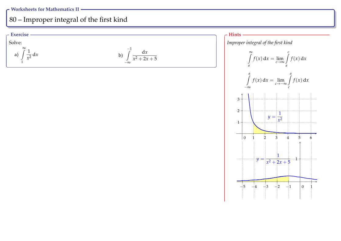
Exercise
Solve:
a)∞∫
1
1x2 dx b)
−1∫−∞
dxx2 + 2x + 5
Hints
Improper integral of the first kind
∞∫a
f (x)dx = limc→∞
c∫a
f (x)dx
a∫−∞
f (x)dx = limc→−∞
a∫c
f (x)dx
0
y =1x2
−1 1 2 3 4 5 6
−1
1
2
3
0
y =1
x2 + 2x + 5
−5 −4 −3 −2 −1 1
−1
1
Worksheets for Mathematics II
81 – Improper integral of the second kind Ry
Definition
Let a function f (x) be continuous and unbounded on the interval [a, b),then the integral
b∫a
f (x)dx = limc→b−
c∫a
f (x)dx = L
is called improper integral of the second kind. If L ∈ R, we say thatthe improper integral is convergent. In the opposite case (L = ∞ orL = −∞) we say that the improper integral is divergent.
Remark
• Quite analogously we define improper integral of the second kindon the interval (a, b].
• We integrate unbounded function on bounded interval.
• If a function f (x) has more points in which it is unbounded, we di-vide the interval into corresponding number of subintervals suchthat every single subinterval contains only one such point. If im-proper integrals are convergent on the subintervals, the integralis convergent on the entire interval, we get it as a sum of partialvalues of single integrals. To check divergence of the improper in-tegral, it is enough that at least one of single integrals is divergent.

Worksheets for Mathematics II
82 – Improper integral of the second kind Ry
Example
Calculate the integral:1∫
0
x√1− x2
dx.
Given function is unbounded on the interval [0, 1), it is improper integral of the second kind:
1∫0
x√1− x2
dx = limc→1−
c∫0
x√1− x2
dx
Substitution:1− x2 = t−2x dx = dt
New limits for t:
lower limit : 0 7→ 1
upper limit : c 7→ 1− c2
After the application:
1∫0
x√1− x2
dx = limc→1−
c∫0
x√1− x2
dx = limc→1−
−12
1−c2∫0
dt√t
= limc→1−
[−√
t]1−c2
1
= limc→1−
(−√
1− c2 + 1)= 1
Improper integral is convergent.
Hints
Improper integral of the second kind
b∫a
f (x)dx = limc→b−
c∫a
f (x)dx
b∫a
f (x)dx = limc→a+
b∫c
f (x)dx
0
y =x√
1− x2
−2 −1 1
−2
−1
1
2
x = −1 x = 1
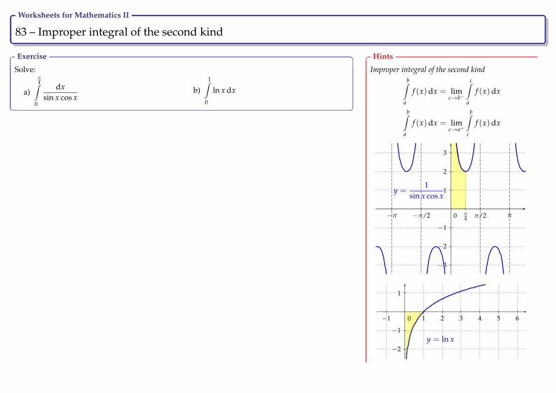
Worksheets for Mathematics II
83 – Improper integral of the second kind Ry
Exercise
Solve:
a)
π4∫
0
dxsin x cos x
b)1∫
0
ln x dx
Hints
Improper integral of the second kindb∫
a
f (x)dx = limc→b−
c∫a
f (x)dx
b∫a
f (x)dx = limc→a+
b∫c
f (x)dx
−4
−3
−2
−1
1
2
3
y =1
sin x cos x
0−π −π/2 ππ/2π4
0
y = ln x
−1 1 2 3 4 5 6
−3
−2
−1
1
Worksheets for Mathematics II
84 – Geometrical application, area of planar regions Ry
If a planar region is surrounded by x-axis, the lines x = a, x = b and thegraph of a continuous non-negative function y = f (x), then area of suchplanar region is determined by a definite integral, it is simply geometricalinterpretation of definite integrals:
P =
b∫a
f (x)dx.
In the case that a function y = f (x) is negative on the interval [a, b], thedefinite integral is also negative. Due to the fact that area must be positivefor arbitrary planar region, we need to add absolute value to guaranteepositivity of the result:
P =
b∫a
| f (x)|dx = −b∫
a
f (x)dx.
If a function y = f (x) is either non-negative or non-positive somewhereon the interval [a, b], then we need to divide the interval on single subin-tervals on which the function is only non-negative or non-positive. Thenwe calculate appropriate areas of such single planar regions. Stress thatnegative results must become positive.

Worksheets for Mathematics II
85 – Geometrical application, area of planar regions Ry
If a planar region is surrounded by graphs of two functions y = f (x) andy = g(x), f (x) ≥ g(x) on the interval [a, b], and the lines x = a, x = b, itsarea is given by:
P =
b∫a
( f (x)− g(x)) dx.
In the case that we do not know integration domain, we have to find outx coordinates of intersection points of both graphs, thus we have to solvethe equation f (x) = g(x).
If a function f is represented by parametric equations x = ϕ(t),y = ψ(t), t ∈ [α, β], where the function ψ(t) is continuous and non-negative on [α, β] and the function ϕ(t) has on the interval [α, β] derivativeϕ(t) different from zero and ϕ(t) is integrable on [α, β], it holds for areaof a planar region surrounded by the graph of such function f on theinterval [α, β]:
P =
∣∣∣∣∣∣β∫
α
ψ(t)ϕ(t)dt
∣∣∣∣∣∣ .

Worksheets for Mathematics II
86 – Area of planar regions Ry
Example
Sketch the graph of the function y = −x3 + 5x + 2 and calculate area of a planar region surrounded by thisgraph, x-axis and the lines x = 1, x = 2.
We sketch the region whose area we are looking for:
0
y = −x3 + 5x + 2
x = 1 x = 2
−4 −3 −2 −1 1 2 3 4
−3
−2
−1
1
2
3
4
5
6
7
We see that the function is non-negative on the interval [1, 2]:
P =
2∫1
(−x3 + 5x + 2)dx =
[−x4
4+
5x2
2+ 2x
]2
1=
(−4 + 10 + 4−
(−1
4+
52+ 2))
=234
.
Hints
Area of a planar region for non-negative function f (x) on [a, b]
P =
b∫a
f (x)dx
Area of a planar region for non-positive function f (x) on [a, b]
P = −b∫
a
f (x)dx
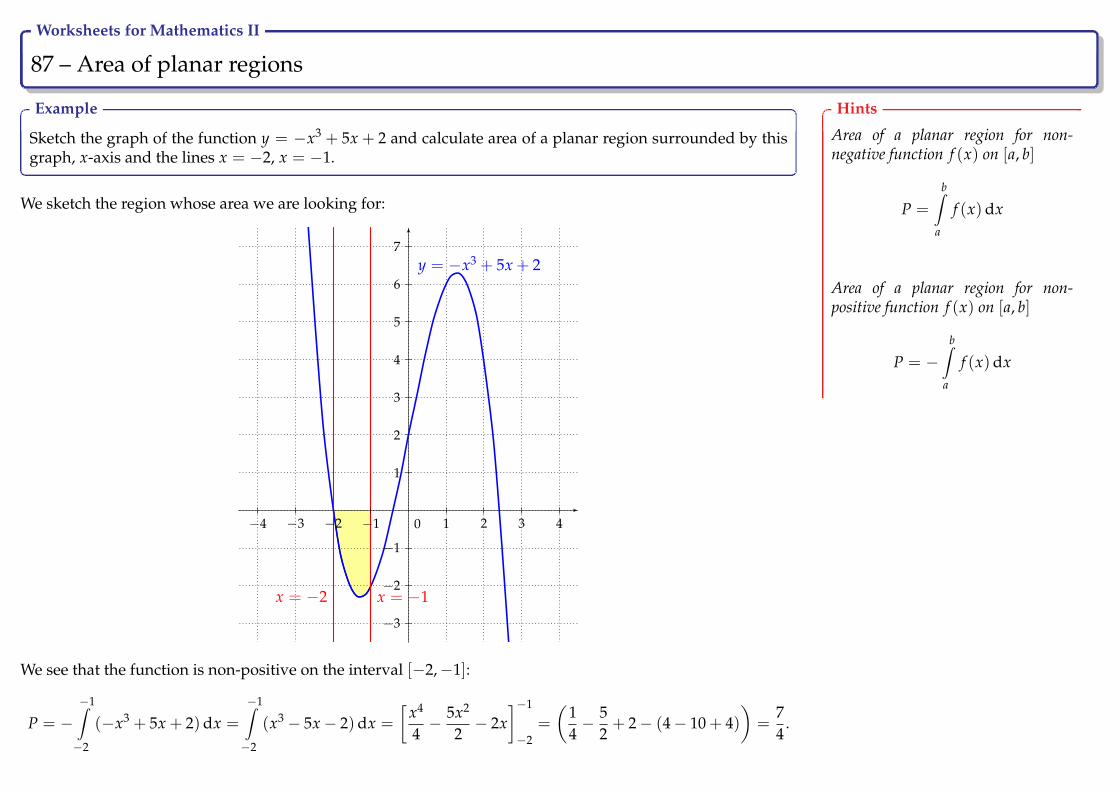
Worksheets for Mathematics II
87 – Area of planar regions Ry
Example
Sketch the graph of the function y = −x3 + 5x + 2 and calculate area of a planar region surrounded by thisgraph, x-axis and the lines x = −2, x = −1.
We sketch the region whose area we are looking for:
0
y = −x3 + 5x + 2
x = −2 x = −1
−4 −3 −2 −1 1 2 3 4
−3
−2
−1
1
2
3
4
5
6
7
We see that the function is non-positive on the interval [−2,−1]:
P = −−1∫−2
(−x3 + 5x + 2)dx =
−1∫−2
(x3 − 5x− 2)dx =
[x4
4− 5x2
2− 2x
]−1
−2=
(14− 5
2+ 2− (4− 10 + 4)
)=
74
.
Hints
Area of a planar region for non-negative function f (x) on [a, b]
P =
b∫a
f (x)dx
Area of a planar region for non-positive function f (x) on [a, b]
P = −b∫
a
f (x)dx
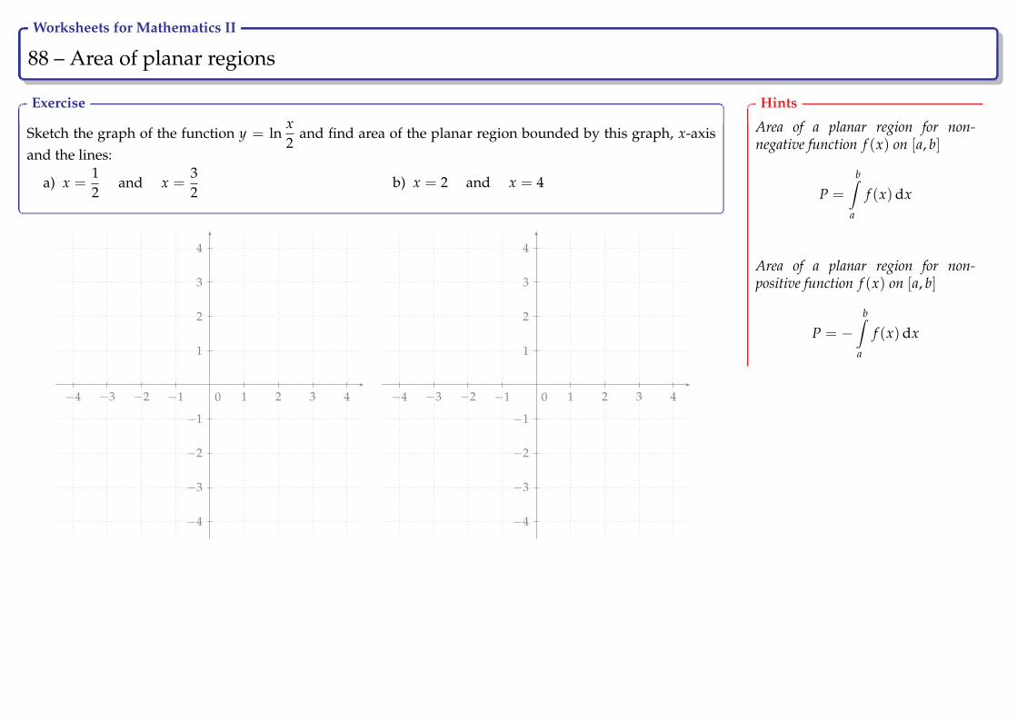
Worksheets for Mathematics II
88 – Area of planar regions Ry
Exercise
Sketch the graph of the function y = lnx2
and find area of the planar region bounded by this graph, x-axisand the lines:
a) x =12
and x =32
b) x = 2 and x = 4
−5 −4 −3 −2 −1 1 2 3 4
−5
−4
−3
−2
−1
1
2
3
4
0 −5 −4 −3 −2 −1 1 2 3 4
−5
−4
−3
−2
−1
1
2
3
4
0
Hints
Area of a planar region for non-negative function f (x) on [a, b]
P =
b∫a
f (x)dx
Area of a planar region for non-positive function f (x) on [a, b]
P = −b∫
a
f (x)dx
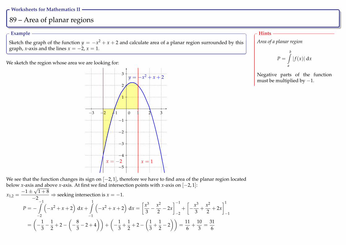
Worksheets for Mathematics II
89 – Area of planar regions Ry
Example
Sketch the graph of the function y = −x2 + x + 2 and calculate area of a planar region surrounded by thisgraph, x-axis and the lines x = −2, x = 1.
We sketch the region whose area we are looking for:
0
y = −x2 + x + 2
x = −2 x = 1
−3 −2 −1 1 2 3
−5
−4
−3
−2
−1
1
2
3
We see that the function changes its sign on [−2, 1], therefore we have to find area of the planar region locatedbelow x-axis and above x-axis. At first we find intersection points with x-axis on [−2, 1]:
x1,2 =−1±
√1 + 8
−2⇒ seeking intersection is x = −1.
P = −−1∫−2
(−x2 + x + 2
)dx +
1∫−1
(−x2 + x + 2
)dx =
[x3
3− x2
2− 2x
]−1
−2+
[−x3
3+
x2
2+ 2x
]1
−1
=
(−1
3− 1
2+ 2−
(−8
3− 2 + 4
))+
(−1
3+
12+ 2−
(13+
12− 2))
=116
+103
=316
Hints
Area of a planar region
P =
b∫a
| f (x)|dx
Negative parts of the functionmust be multiplied by −1.
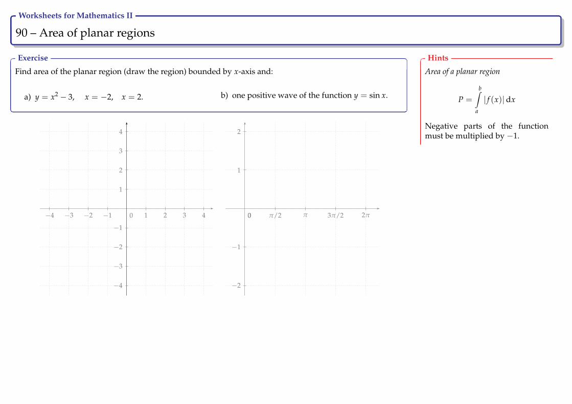
Worksheets for Mathematics II
90 – Area of planar regions Ry
Exercise
Find area of the planar region (draw the region) bounded by x-axis and:
a) y = x2 − 3, x = −2, x = 2. b) one positive wave of the function y = sin x.
−5 −4 −3 −2 −1 1 2 3 4
−4
−3
−2
−1
1
2
3
4
0
−2
−1
1
2
0 3π/2ππ/2 2π0
Hints
Area of a planar region
P =
b∫a
| f (x)|dx
Negative parts of the functionmust be multiplied by −1.
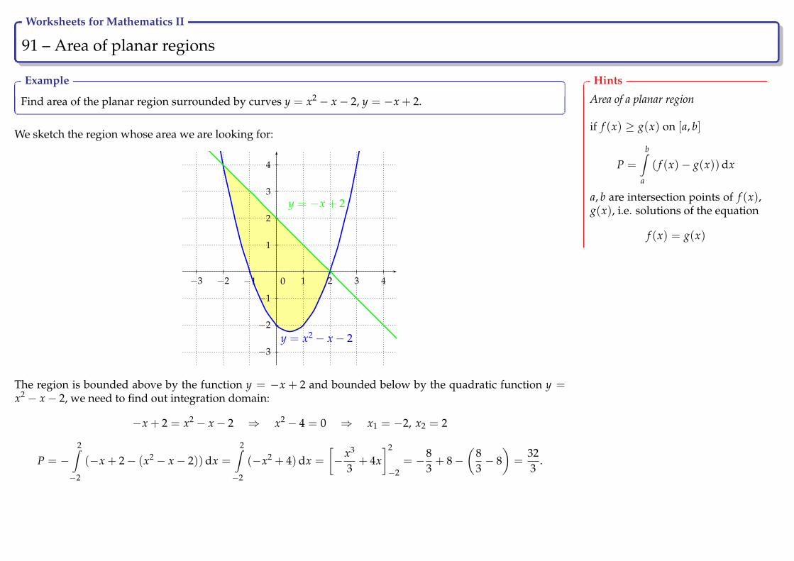
Worksheets for Mathematics II
91 – Area of planar regions Ry
Example
Find area of the planar region surrounded by curves y = x2 − x− 2, y = −x + 2.
We sketch the region whose area we are looking for:
0
y = x2 − x− 2
y = −x + 2
−3 −2 −1 1 2 3 4
−3
−2
−1
1
2
3
4
The region is bounded above by the function y = −x + 2 and bounded below by the quadratic function y =x2 − x− 2, we need to find out integration domain:
−x + 2 = x2 − x− 2 ⇒ x2 − 4 = 0 ⇒ x1 = −2, x2 = 2
P = −2∫−2
(−x + 2− (x2 − x− 2))dx =
2∫−2
(−x2 + 4)dx =
[−x3
3+ 4x
]2
−2= −8
3+ 8−
(83− 8)=
323
.
Hints
Area of a planar region
if f (x) ≥ g(x) on [a, b]
P =
b∫a
( f (x)− g(x))dx
a, b are intersection points of f (x),g(x), i.e. solutions of the equation
f (x) = g(x)
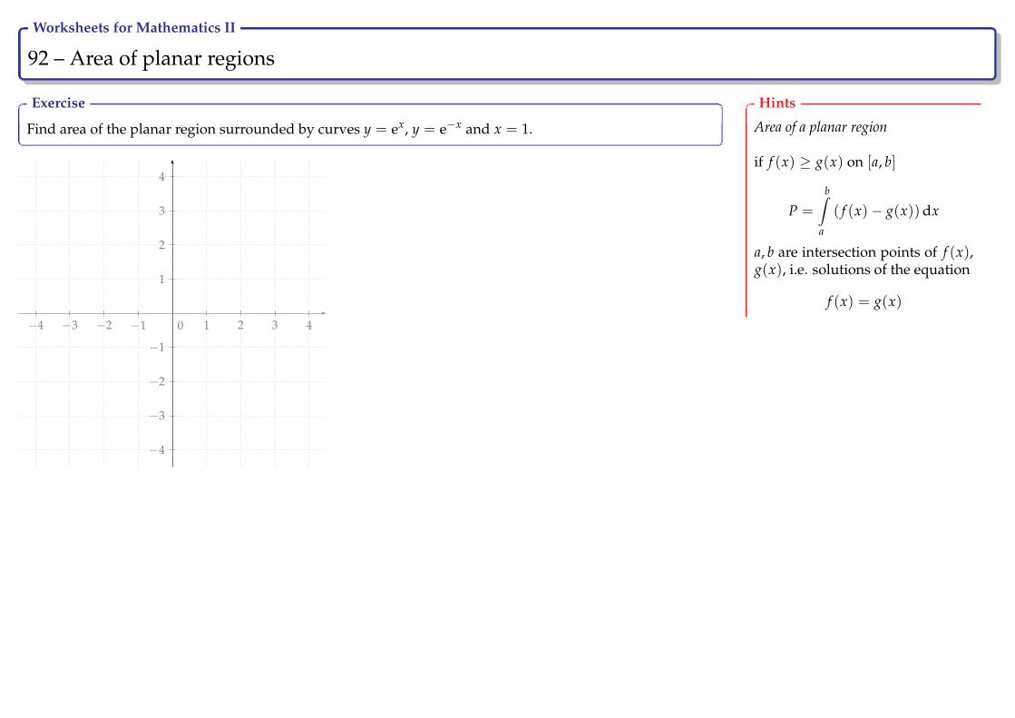
Worksheets for Mathematics II
92 – Area of planar regions Ry
Exercise
Find area of the planar region surrounded by curves y = ex, y = e−x and x = 1.
−5 −4 −3 −2 −1 1 2 3 4
−4
−3
−2
−1
1
2
3
4
0
Hints
Area of a planar region
if f (x) ≥ g(x) on [a, b]
P =
b∫a
( f (x)− g(x))dx
a, b are intersection points of f (x),g(x), i.e. solutions of the equation
f (x) = g(x)

Worksheets for Mathematics II
93 – Area of planar regions Ry
Exercise
Find area of the planar region surrounded by curves y = x2 + 1, y = 2x2 − 3.
−5 −4 −3 −2 −1 1 2 3 4
−4
−3
−2
−1
1
2
3
4
0
Hints
Area of a planar region
if f (x) ≥ g(x) on [a, b]
P =
b∫a
( f (x)− g(x))dx
a, b are intersection points of f (x),g(x), i.e. solutions of the equation
f (x) = g(x)
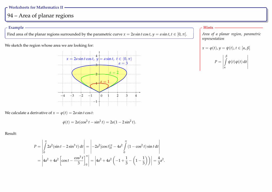
Worksheets for Mathematics II
94 – Area of planar regions Ry
Example
Find area of the planar regions surrounded by the parametric curve x = 2a sin t cos t, y = a sin t, t ∈ [0, π].
We sketch the region whose area we are looking for:
0
a = 1
a = 2
a = 3x = 2a sin t cos t, y = a sin t, t ∈ 〈0, π〉
−4 −3 −2 −1 1 2 3 4
−1
1
2
3
4
We calculate a derivative of x = ϕ(t) = 2a sin t cos t:
ϕ(t) = 2a(cos2 t− sin2 t) = 2a(1− 2 sin2 t).
Result:
P =
∣∣∣∣∣∣π∫
0
2a2(sin t− 2 sin3 t)dt
∣∣∣∣∣∣ =∣∣∣∣∣∣−2a2[cos t]π0 − 4a2
π∫0
(1− cos2 t) sin t dt
∣∣∣∣∣∣=
∣∣∣∣∣4a2 + 4a2[
cos t− cos3 t3
]π
0
∣∣∣∣∣ =∣∣∣∣4a2 + 4a2
(−1 +
13−(
1− 13
))∣∣∣∣ = 43
a2.
Hints
Area of a planar region, parametricrepresentation
x = ϕ(t), y = ψ(t), t ∈ [α, β]
P =
∣∣∣∣∣∣β∫
α
ψ(t)ϕ(t)dt
∣∣∣∣∣∣
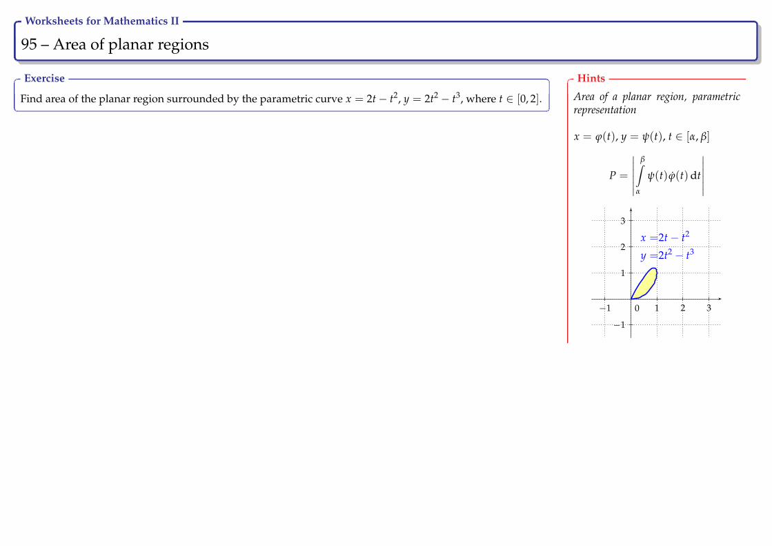
Worksheets for Mathematics II
95 – Area of planar regions Ry
Exercise
Find area of the planar region surrounded by the parametric curve x = 2t− t2, y = 2t2 − t3, where t ∈ [0, 2].
Hints
Area of a planar region, parametricrepresentation
x = ϕ(t), y = ψ(t), t ∈ [α, β]
P =
∣∣∣∣∣∣β∫
α
ψ(t)ϕ(t)dt
∣∣∣∣∣∣
0
x =2t− t2
y =2t2 − t3
−1 1 2 3
−1
1
2
3

Worksheets for Mathematics II
96 – Length of planar curves Ry
Theorem
If a function y = f (x) is defined and has continuous derivative on theinterval [a, b], then for length of its graph holds:
l =b∫
a
√1 + ( f ′(x))2 dx.
Let us take a closer look on a more general case when a curve does nothave to be the graph of a function, e.g. it may be a trajectory of a pointcontinuously moving in the plane. Such curve is represented by paramet-ric equations
x = ϕ(t), y = ψ(t),
where t ∈ [α, β]. From the physical point of view length of a curve is apath along which the point passes from time moment α to time moment β.For length of parametric curves holds:
l =
β∫α
√(ϕ(t))2 + (ψ(t))2 dt.

Worksheets for Mathematics II
97 – Length of planar curves Ry
Example
Find length of the curve y = arcsin x +√
1− x2 for 0 ≤ x ≤ 1.
We sketch the curve whose length we are looking for:
y = arcsin(x) +√
1− x2, x ∈ [0, 1]
0−1 1 2
−1
1
2
We calculate a derivative and its square:
( f ′(x))2 =
(1√
1− x2− 2x
2√
1− x2
)2
=1− x1 + x
.
Result:
l =1∫
0
√1 +
1− x1 + x
dx =
1∫0
√1 + x + 1− x
1 + xdx =
1∫0
√2√
1 + xdx =
√2
1∫0
(1+ x)−12 dx =
√2
[(1 + x)
12
12
]1
0
= 4− 2√
2.
Hints
Length of a planar curve
l =b∫
a
√1 + ( f ′(x))2 dx
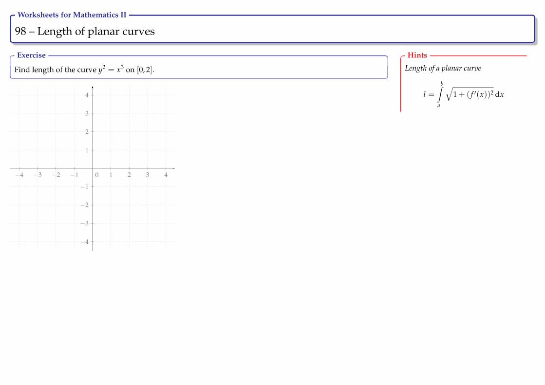
Worksheets for Mathematics II
98 – Length of planar curves Ry
Exercise
Find length of the curve y2 = x3 on [0, 2].
−5 −4 −3 −2 −1 1 2 3 4
−4
−3
−2
−1
1
2
3
4
0
Hints
Length of a planar curve
l =b∫
a
√1 + ( f ′(x))2 dx

Worksheets for Mathematics II
99 – Length of planar curves Ry
Exercise
Find length of the curve y = ln sin x forπ
4≤ x ≤ π
2.
−5 −4 −3 −2 −1 1 2 3 4
−4
−3
−2
−1
1
2
3
4
0
Hints
Length of a planar curve
l =b∫
a
√1 + ( f ′(x))2 dx
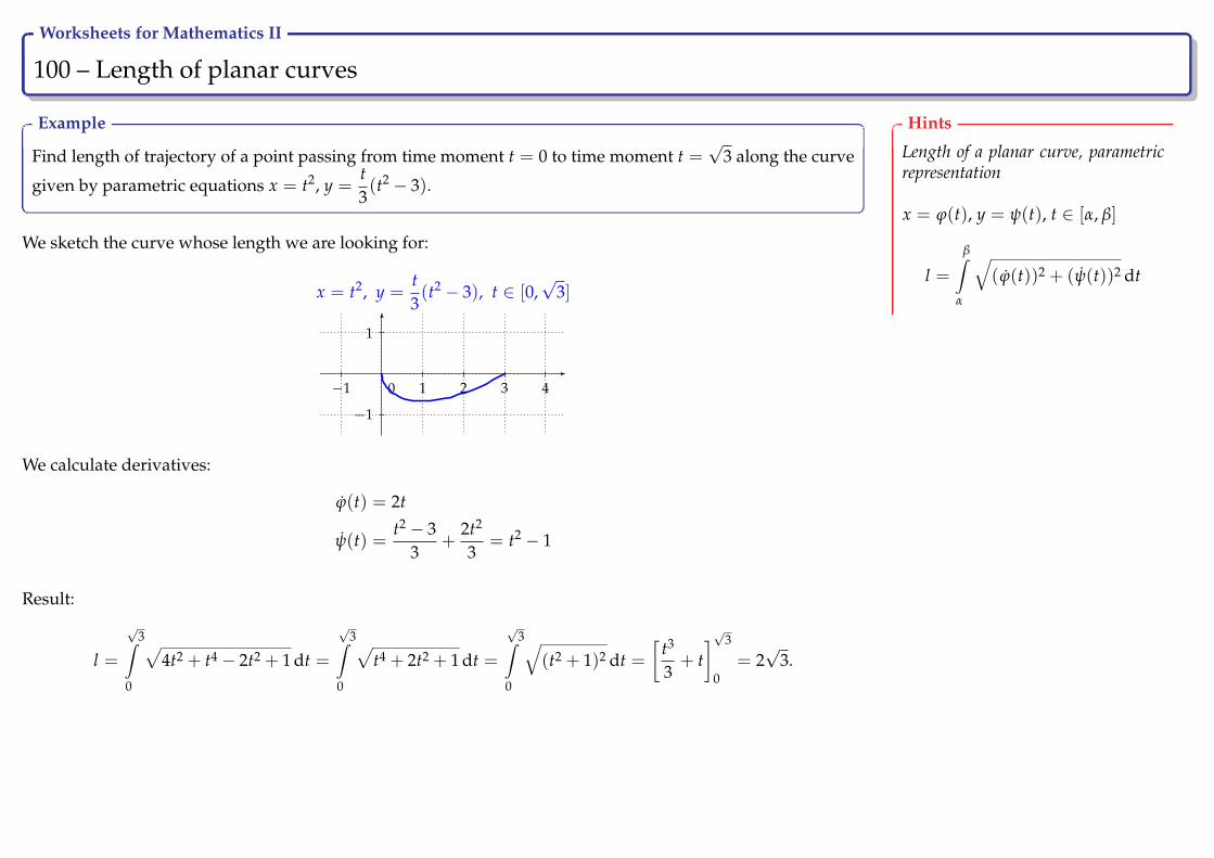
Worksheets for Mathematics II
100 – Length of planar curves Ry
Example
Find length of trajectory of a point passing from time moment t = 0 to time moment t =√
3 along the curve
given by parametric equations x = t2, y =t3(t2 − 3).
We sketch the curve whose length we are looking for:
x = t2, y =t3(t2 − 3), t ∈ [0,
√3]
0−1 1 2 3 4
−1
1
We calculate derivatives:
ϕ(t) = 2t
ψ(t) =t2 − 3
3+
2t2
3= t2 − 1
Result:
l =
√3∫
0
√4t2 + t4 − 2t2 + 1 dt =
√3∫
0
√t4 + 2t2 + 1 dt =
√3∫
0
√(t2 + 1)2 dt =
[t3
3+ t]√3
0= 2√
3.
Hints
Length of a planar curve, parametricrepresentation
x = ϕ(t), y = ψ(t), t ∈ [α, β]
l =
β∫α
√(ϕ(t))2 + (ψ(t))2 dt
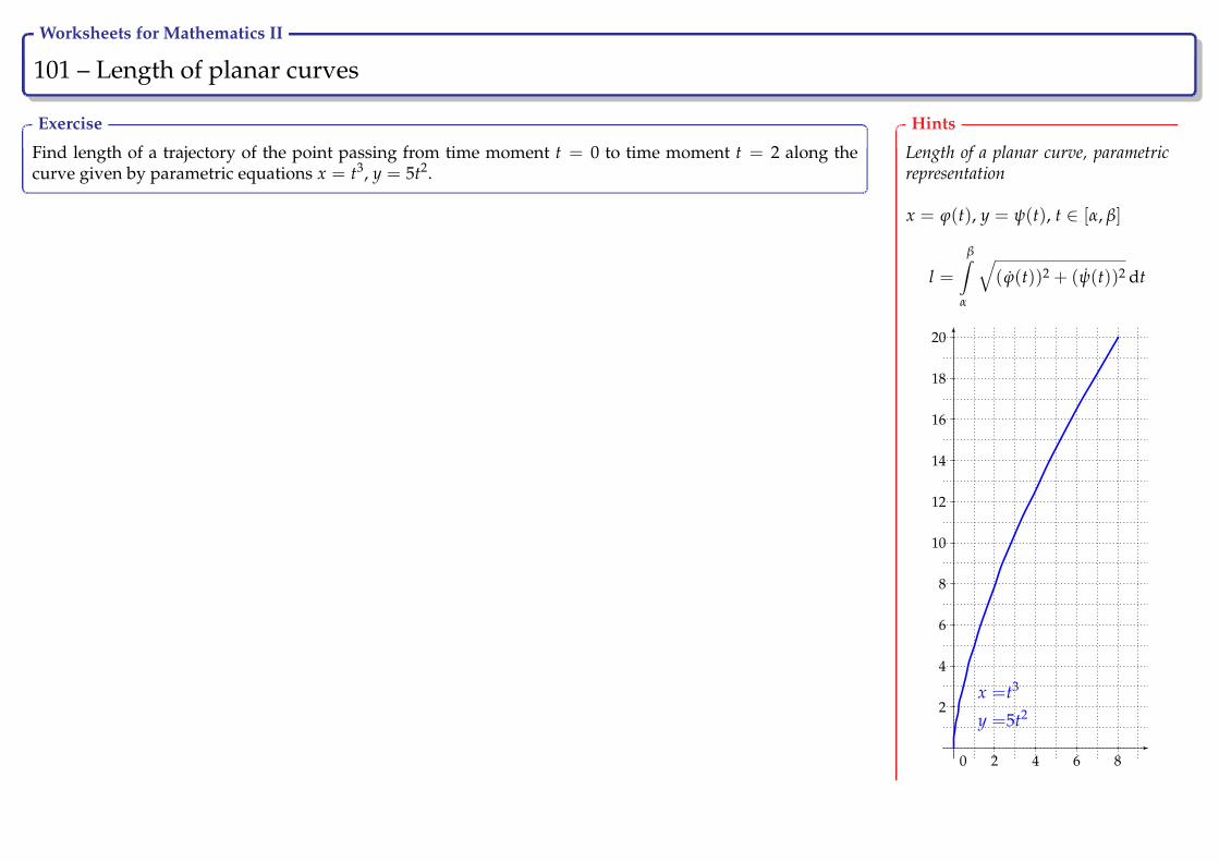
Worksheets for Mathematics II
101 – Length of planar curves Ry
Exercise
Find length of a trajectory of the point passing from time moment t = 0 to time moment t = 2 along thecurve given by parametric equations x = t3, y = 5t2.
Hints
Length of a planar curve, parametricrepresentation
x = ϕ(t), y = ψ(t), t ∈ [α, β]
l =
β∫α
√(ϕ(t))2 + (ψ(t))2 dt
0
x =t3
y =5t2
2 4 6 8
2
4
6
8
10
12
14
16
18
20
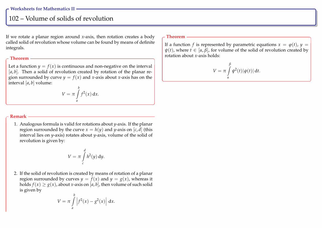
Worksheets for Mathematics II
102 – Volume of solids of revolution Ry
If we rotate a planar region around x-axis, then rotation creates a bodycalled solid of revolution whose volume can be found by means of definiteintegrals.
Theorem
Let a function y = f (x) is continuous and non-negative on the interval[a, b]. Then a solid of revolution created by rotation of the planar re-gion surrounded by curve y = f (x) and x-axis about x-axis has on theinterval [a, b] volume:
V = π
b∫a
f 2(x)dx.
Remark
1. Analogous formula is valid for rotations about y-axis. If the planarregion surrounded by the curve x = h(y) and y-axis on [c, d] (thisinterval lies on y-axis) rotates about y-axis, volume of the solid ofrevolution is given by:
V = π
d∫c
h2(y)dy.
2. If the solid of revolution is created by means of rotation of a planarregion surrounded by curves y = f (x) and y = g(x), whereas itholds f (x) ≥ g(x), about x-axis on [a, b], then volume of such solidis given by
V = π
b∫a
∣∣∣ f 2(x)− g2(x)∣∣∣ dx.
Theorem
If a function f is represented by parametric equations x = ϕ(t), y =ψ(t), where t ∈ [α, β], for volume of the solid of revolution created byrotation about x-axis holds:
V = π
β∫α
ψ2(t)|ϕ(t)|dt.
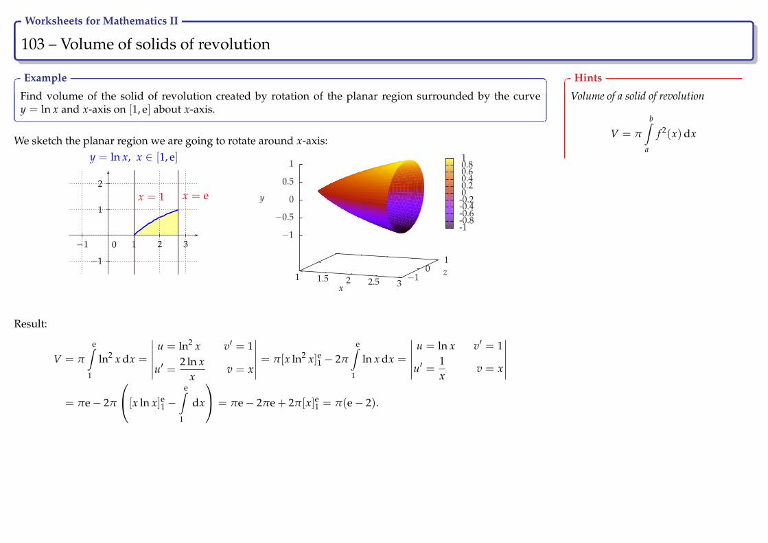
Worksheets for Mathematics II
103 – Volume of solids of revolution Ry
Example
Find volume of the solid of revolution created by rotation of the planar region surrounded by the curvey = ln x and x-axis on [1, e] about x-axis.
We sketch the planar region we are going to rotate around x-axis:
0
y = ln x, x ∈ [1, e]
x = 1 x = e
−1 1 2 3
−1
1
2
1 1.5 2 2.5 3−1
0
1
−1
−0.5
0
0.5
1
x
z
y
-1-0.8-0.6-0.4-0.200.20.40.60.81
Result:
V = π
e∫1
ln2 x dx =
∣∣∣∣∣∣u = ln2 x v′ = 1
u′ =2 ln x
xv = x
∣∣∣∣∣∣ = π[x ln2 x]e1 − 2π
e∫1
ln x dx =
∣∣∣∣∣∣u = ln x v′ = 1
u′ =1x
v = x
∣∣∣∣∣∣= πe− 2π
[x ln x]e1 −e∫
1
dx
= πe− 2πe + 2π[x]e1 = π(e− 2).
Hints
Volume of a solid of revolution
V = π
b∫a
f 2(x)dx

Worksheets for Mathematics II
104 – Volume of solids of revolution Ry
Exercise
Find volume of the solid of revolution created by rotation of the planar region surrounded by the curvey =√
2x− 3 and x-axis on [2, 3] about x-axis.
−5 −4 −3 −2 −1 1 2 3 4
−4
−3
−2
−1
1
2
3
4
0
Hints
Volume of a solid of revolution
V = π
b∫a
f 2(x)dx
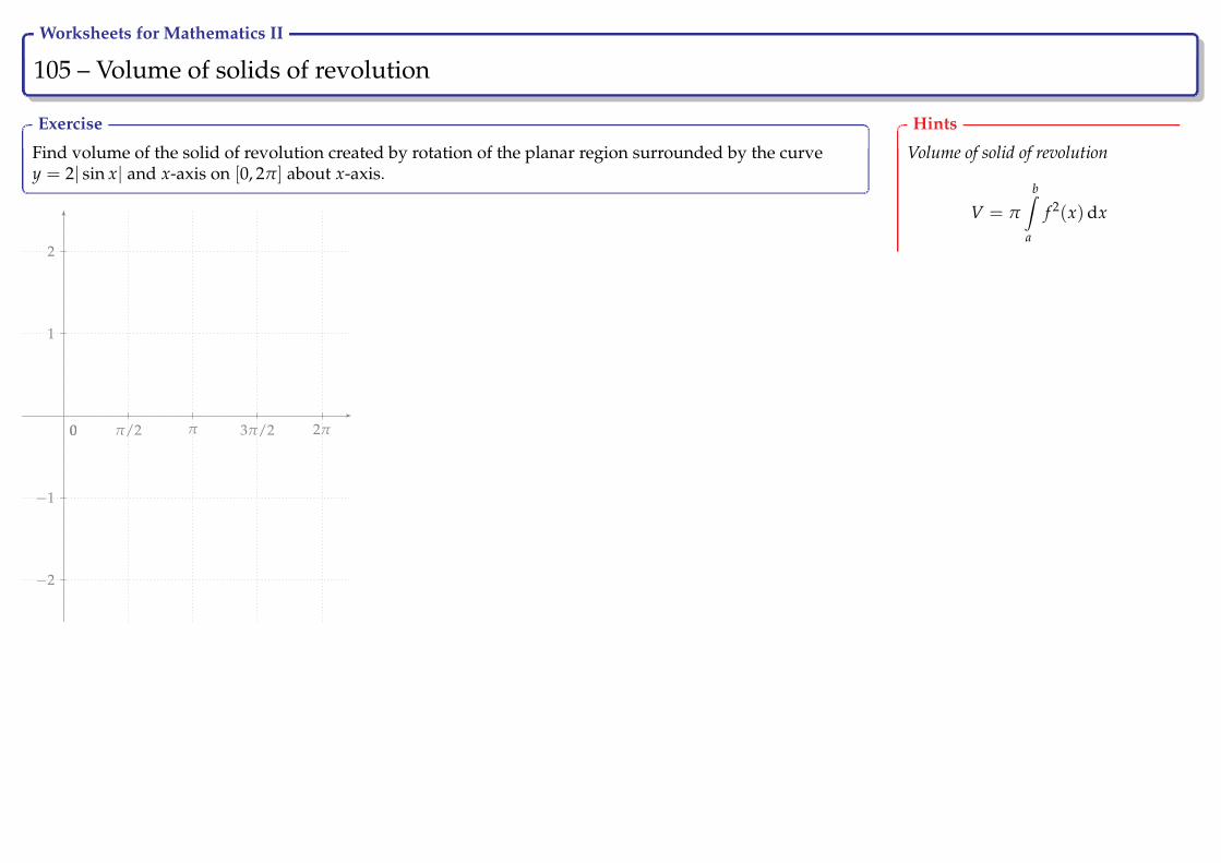
Worksheets for Mathematics II
105 – Volume of solids of revolution Ry
Exercise
Find volume of the solid of revolution created by rotation of the planar region surrounded by the curvey = 2| sin x| and x-axis on [0, 2π] about x-axis.
−2
−1
1
2
0 3π/2ππ/2 2π0
Hints
Volume of solid of revolution
V = π
b∫a
f 2(x)dx

Worksheets for Mathematics II
106 – Volume of solids of revolution Ry
Example
Find volume of the solid of revolution created by rotation of the planar region surrounded by the curvesy = ex, y = −2e−x + 3 about x-axis.
We sketch the planar region we are going to rotate about x-axis:
0
y = ex
y = −2e−x + 3x = 0
x = ln 2−1 1 2
1
2
0 1−2−1
01
2
−2
−1.5
−1
−0.5
0
0.5
1
1.5
2
xz
y
-2
-1.5
-1
-0.5
0
0.5
1
1.5
2
We find intersection points to get integration domain:
−2e−x + 3 = ex ⇒ 2ex − 3 + ex = 0⇒ 2− 3ex + e2x
ex = 0⇒ 2− 3ex + e2x = 0,
we use the substitution ex = t and solve the quadratic equation t2 − 3t + 2 = 0⇒ x1 = 0, x2 = ln 2.
V = π
ln 2∫0
∣∣∣(−2e−x + 3)2 − e2x∣∣∣ dx = π
ln 2∫0
(4e−2x − 12e−x + 9− e2x)dx
= π
[−2e−2x + 12e−x + 9x− e2x
2
]ln 2
0= π(9 ln 2− 6).
Hints
Volume of a solid of revolution
V = π
b∫a
∣∣∣ f 2(x)− g2(x)∣∣∣ dx,
where a, b are intersection points
we solve the equation f (x) = g(x)

Worksheets for Mathematics II
107 – Volume of solids of revolution Ry
Exercise
Find volume of the solid of revolution created by rotation of the planar region surrounded by the curvesy = x2, y2 = x about x-axis.
−5 −4 −3 −2 −1 1 2 3 4
−4
−3
−2
−1
1
2
3
4
0
Hints
Volume of solid of revolution
V = π
b∫a
∣∣∣ f 2(x)− g2(x)∣∣∣ dx,
where a, b are intersection points
we solve the equation f (x) = g(x)
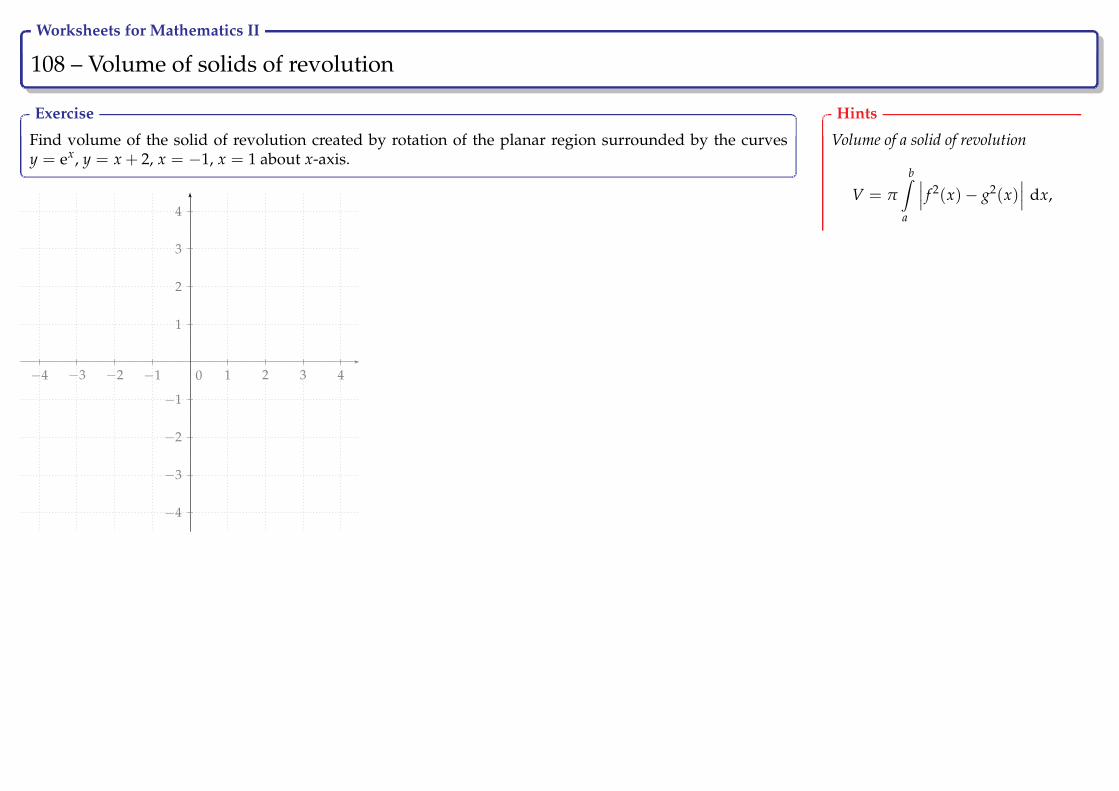
Worksheets for Mathematics II
108 – Volume of solids of revolution Ry
Exercise
Find volume of the solid of revolution created by rotation of the planar region surrounded by the curvesy = ex, y = x + 2, x = −1, x = 1 about x-axis.
−5 −4 −3 −2 −1 1 2 3 4
−4
−3
−2
−1
1
2
3
4
0
Hints
Volume of a solid of revolution
V = π
b∫a
∣∣∣ f 2(x)− g2(x)∣∣∣ dx,
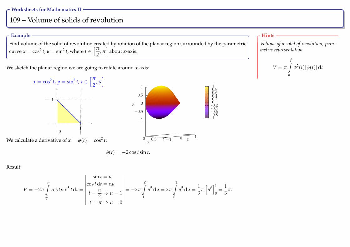
Worksheets for Mathematics II
109 – Volume of solids of revolution Ry
Example
Find volume of the solid of revolution created by rotation of the planar region surrounded by the parametric
curve x = cos2 t, y = sin2 t, where t ∈[π
2, π]
about x-axis.
We sketch the planar region we are going to rotate around x-axis:
x = cos2 t, y = sin2 t, t ∈[π
2, π]
0−1 1
−1
1
0 0.5 1 −1 0 1
−1
−0.5
0
0.5
1
xz
y
-1-0.8-0.6-0.4-0.200.20.40.60.81
We calculate a derivative of x = ϕ(t) = cos2 t:
ϕ(t) = −2 cos t sin t.
Result:
V = −2π
π∫π2
cos t sin5 t dt =
∣∣∣∣∣∣∣∣∣∣
sin t = ucos t dt = du
t =π
2⇒ u = 1
t = π ⇒ u = 0
∣∣∣∣∣∣∣∣∣∣= −2π
0∫1
u5 du = 2π
1∫0
u5 du =13
π[u6]1
0=
13
π.
Hints
Volume of a solid of revolution, para-metric representation
V = π
β∫α
ψ2(t)|ϕ(t)|dt

Worksheets for Mathematics II
110 – Volume of solids of revolution Ry
Exercise
Find volume of the solid of revolution created by rotation of a planar region surrounded by the parametric
curve x =1− t1 + t
, y =1
1 + t, where t ∈ [0, 1] about x-axis.
Hints
Volume of a solid of revolution, para-metric representation
V = π
β∫α
ψ2(t)|ϕ(t)|dt

Worksheets for Mathematics II
111 – Lateral surface of solids of revolution Ry
Theorem
Let a function y = f (x) be continuous and non-negative on the interval[a, b] with continuous derivative. Then for lateral surface created byrotation of the curve y = f (x) about x-axis and its lateral surface areaholds on the interval [a, b]:
S = 2π
b∫a
f (x)√
1 + ( f ′(x))2 dx.
Remark
Rotation about y-axis:
S = 2π
d∫c
h(y)√
1 + (h′(y))2 dy.
Theorem
If a function y = f (x) is represented by parametric equations x = ϕ(t),y = ψ(t), where t ∈ [α, β], for lateral surface created by rotation of suchfunction about x-axis and its lateral surface area holds:
S = 2π
β∫α
ψ(t)√(ϕ(t))2 + (ψ(t))2 dt, ψ(t) ≥ 0.

Worksheets for Mathematics II
112 – Lateral surface of solids of revolution Ry
Example
Find lateral surface area of the solid revolution created by rotation of the planar region surrounded by thecurve y = 2
√x and x-axis on x ∈ [0, 2] about x-axis.
We sketch the planar region we are going to rotate about x-axis:
0
y = 2√
x, t ∈ [0, 2]
1 2
1
2
3
0 1 2 3−4−2
02
4
−3
−2
−1
0
1
2
3
x
z
y
-3
-2
-1
0
1
2
3
We calculate the second power of a derivative:
(y′)2 =1x
.
Result:
S = 4π
2∫0
√x
√1 +
1x
dx = 4π
2∫0
√x
√x + 1
xdx = 4π
2∫0
√x + 1 dx =
83
π[(x + 1)
32
]2
0=
83
π(√
27− 1).
Hints
Lateral surface area
S = 2π
b∫a
f (x)√
1 + ( f ′(x))2 dx,
for f (x) ≥ 0
Worksheets for Mathematics II
113 – Lateral surface of solids of revolution Ry
Exercise
Find lateral surface area of the solid of revolution created by rotation of the planar region surrounded by thecurve y =
√x and x-axis on [1, 4] about x-axis.
Hints
Lateral surface area
S = 2π
b∫a
f (x)√
1 + ( f ′(x))2 dx,
for f (x) ≥ 0

Worksheets for Mathematics II
114 – Lateral surface of solids of revolution Ry
Example
Find lateral surface area of the solid of revolution created by rotation of the planar region surrounded by the
parametric curve x = cos2 t, y = sin2 t on[0,
π
2
]about x-axis.
We sketch the planar region we are going to rotate about x-axis:
x = cos2 t, y = sin2 t, t ∈[π
2, π]
0−1 1
−1
1
0 0.5 1 −1 0 1
−1
−0.5
0
0.5
1
xz
y
-1-0.8-0.6-0.4-0.200.20.40.60.81
We calculate second powers of derivatives:
(ϕ(t))2 = 4 cos2 t sin2 t
(ψ(t))2 = 4 cos2 t sin2 t
Result:
S = 2π
π2∫
0
sin2 t√
8 cos2 t sin2 t dt = 2π√
8
π2∫
0
cos t sin3 t dt =
∣∣∣∣∣∣∣∣∣∣
sin t = ucos t dt = du
t = 0⇒ u = 0
t =π
2⇒ u = 1
∣∣∣∣∣∣∣∣∣∣= 2π
√8
1∫0
u3 du
= π√
2[u4]1
0= π√
2.
Hints
Lateral surface area, parametric repre-sentation
S = 2π
β∫α
ψ(t)√(ϕ(t))2 + (ψ(t))2 dt
for ψ(t) ≥ 0
Worksheets for Mathematics II
115 – Lateral surface of solids of revolution Ry
Exercise
Find lateral surface area of the solid of revolution created by rotation of the planar region surrounded by theparametric curve x = a sin 2t, y = 2a sin2 t on [0, π] about x-axis.
Hints
Lateral surface area, parametric repre-sentation
S = 2π
β∫α
ψ(t)√(ϕ(t))2 + (ψ(t))2 dt
for ψ(t) ≥ 0
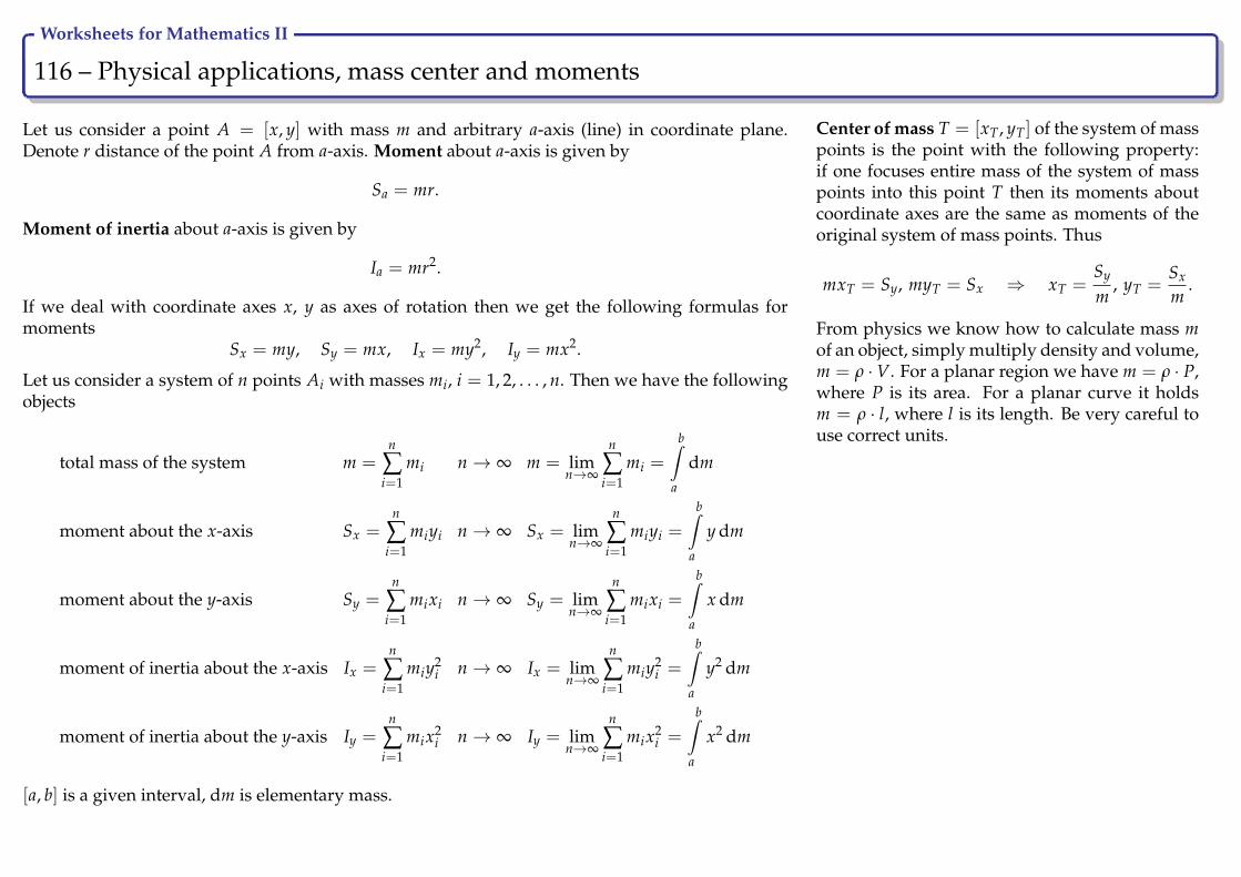
Worksheets for Mathematics II
116 – Physical applications, mass center and moments Ry
Let us consider a point A = [x, y] with mass m and arbitrary a-axis (line) in coordinate plane.Denote r distance of the point A from a-axis. Moment about a-axis is given by
Sa = mr.
Moment of inertia about a-axis is given by
Ia = mr2.
If we deal with coordinate axes x, y as axes of rotation then we get the following formulas formoments
Sx = my, Sy = mx, Ix = my2, Iy = mx2.
Let us consider a system of n points Ai with masses mi, i = 1, 2, . . . , n. Then we have the followingobjects
total mass of the system m =n
∑i=1
mi n→ ∞ m = limn→∞
n
∑i=1
mi =
b∫a
dm
moment about the x-axis Sx =n
∑i=1
miyi n→ ∞ Sx = limn→∞
n
∑i=1
miyi =
b∫a
y dm
moment about the y-axis Sy =n
∑i=1
mixi n→ ∞ Sy = limn→∞
n
∑i=1
mixi =
b∫a
x dm
moment of inertia about the x-axis Ix =n
∑i=1
miy2i n→ ∞ Ix = lim
n→∞
n
∑i=1
miy2i =
b∫a
y2 dm
moment of inertia about the y-axis Iy =n
∑i=1
mix2i n→ ∞ Iy = lim
n→∞
n
∑i=1
mix2i =
b∫a
x2 dm
[a, b] is a given interval, dm is elementary mass.
Center of mass T = [xT, yT] of the system of masspoints is the point with the following property:if one focuses entire mass of the system of masspoints into this point T then its moments aboutcoordinate axes are the same as moments of theoriginal system of mass points. Thus
mxT = Sy, myT = Sx ⇒ xT =Sy
m, yT =
Sx
m.
From physics we know how to calculate mass mof an object, simply multiply density and volume,m = ρ ·V. For a planar region we have m = ρ · P,where P is its area. For a planar curve it holdsm = ρ · l, where l is its length. Be very careful touse correct units.

Worksheets for Mathematics II
117 – Homogeneous curves Ry
Theorem
Let a curve is given by explicit equation y = f (x) with continuousderivative f ′(x) on [a, b]. Let density ρ of the curve is constant. Mass ofthe curve is given by
m =
b∫a
dm = ρ
b∫a
dl = ρ
b∫a
√1 + ( f ′(x))2 dx.
For moments about coordinate axes hold,
Sx =
b∫a
y dm = ρ
b∫a
f (x)√
1 + ( f ′(x))2 dx,
Sy =
b∫a
x dm = ρ
b∫a
x√
1 + ( f ′(x))2 dx.
For moments of inertia about coordinate axes hold,
Ix =
b∫a
y2dm = ρ
b∫a
f 2(x)√
1 + ( f ′(x))2 dx,
Iy =
b∫a
x2 dm = ρ
b∫a
x2√
1 + ( f ′(x))2 dx.
Mass center coordinates, T = [xT, yT]
xT =Sy
m=
b∫a
x√
1 + ( f ′(x))2 dx
b∫a
√1 + ( f ′(x))2 dx
, yT =Sx
m=
b∫a
f (x)√
1 + ( f ′(x))2 dx
b∫a
√1 + ( f ′(x))2 dx
Theorem
Consider a curve represented by parametric equations x = ϕ(t), y =ψ(t) on [α, β], ψ(t) ≥ 0. The functions ϕ(t), ψ(t) have continuousderivatives on [α, β], ϕ(t) > 0. If density ρ is constant, then the curvehas mass
m =
β∫α
dm = ρ
β∫α
dl = ρ
β∫α
√ϕ2(t) + ψ2(t)dt.
For moments about coordinate axes hold,
Sx =
β∫α
y dm = ρ
β∫α
ψ(t)√
ϕ2(t) + ψ2(t)dt,
Sy =
β∫α
x dm = ρ
β∫α
ϕ(t)√
ϕ2(t) + ψ2(t)dt.
For moments of inertia about coordinate axes hold,
Ix =
β∫α
y2dm = ρ
β∫α
ψ2(t)√
ϕ2(t) + ψ2(t)dt,
Iy =
β∫α
x2 dm = ρ
β∫α
ϕ2(t)√
ϕ2(t) + ψ2(t)dt.
Mass center coordinates, T = [xT, yT], xT = Sy/m, yT = Sx/m,
xT =
β∫α
ϕ(t)√
ϕ2(t) + ψ2(t)dt
β∫α
√ϕ2(t) + ψ2(t)dt
, yT =
β∫α
ψ(t)√
ϕ2(t) + ψ2(t)dt
β∫α
√ϕ2(t) + ψ2(t)dt

Worksheets for Mathematics II
118 – Homogeneous curves Ry
Example
Find center of mass of homogeneous half-circle represented by parametric equations x = r cos t,y = r sin t, t ∈ [0, π].
We sketch the curve whose center of mass we are looking for:x = r cos t, y = r sin t, t ∈ [0, π]
0−2 −1 1 2
−1
1T
We calculate derivatives:ϕ(t) = −r sin t, ψ(t) = r cos t.
We calculate mass of the curve:
m = ρ
π∫0
√r2 sin2 t + r2 cos2 t dt = ρ
π∫0
√r2(sin2 t + cos2 t)dt = ρr
π∫0
dt = ρr[t]π0 = ρπr.
For moments about coordinate axes we have:
Sx = ρ
π∫0
r sin t√
r2 sin2 t + r2 cos2 t dt = ρr2π∫
0
sin t dt = ρr2[− cos t]π0 = 2ρr2,
Sy = ρ
π∫0
r cos t√
r2 sin2 t + r2 cos2 t dt = ρr2π∫
0
cos t dt = ρr2[sin t]π0 = 0.
Center of mass coordinates:
xT =Sy
m=
0ρπr
= 0, yT =Sx
m=
2ρr2
ρπr=
2rπ
⇒ T =
[0,
2rπ
].
Hints
Planar homogeneous curve
x = ϕ(t), y = ψ(t), t ∈ [α, β]
Mass
m = ρ
β∫α
√ϕ2(t) + ψ2(t)dt
Moments about coordinate axes
Sx =
β∫α
y dm = ρ
β∫α
ψ(t)√
ϕ2(t) + ψ2(t)dt
Sy =
β∫α
x dm = ρ
β∫α
ϕ(t)√
ϕ2(t) + ψ2(t)dt
Mass center coordinates, T = [xT, yT]
xT =Sy
m=
β∫α
ϕ(t)√
ϕ2(t) + ψ2(t)dt
β∫α
√ϕ2(t) + ψ2(t)dt
yT =Sx
m=
β∫α
ψ(t)√
ϕ2(t) + ψ2(t)dt
β∫α
√ϕ2(t) + ψ2(t)dt
Worksheets for Mathematics II
119 – Homogeneous curves Ry
Exercise
Find center of mass of the homogeneous curve represented by parametric equations
x = t2, y = t− t3
3, t ∈ [0,
√3].
Hints
Planar homogeneous curve
x = ϕ(t), y = ψ(t), t ∈ [α, β]
Mass
m = ρ
β∫α
√ϕ2(t) + ψ2(t)dt
Moments about coordinate axes
Sx =
β∫α
y dm = ρ
β∫α
ψ(t)√
ϕ2(t) + ψ2(t)dt
Sy =
β∫α
x dm = ρ
β∫α
ϕ(t)√
ϕ2(t) + ψ2(t)dt
Mass center coordinates, T = [xT, yT]
xT =Sy
m=
β∫α
ϕ(t)√
ϕ2(t) + ψ2(t)dt
β∫α
√ϕ2(t) + ψ2(t)dt
yT =Sx
m=
β∫α
ψ(t)√
ϕ2(t) + ψ2(t)dt
β∫α
√ϕ2(t) + ψ2(t)dt

Worksheets for Mathematics II
120 – Homogeneous curves Ry
Exercise
Find center of mass of the homogeneous curve given by f (x) = −x2
2+ 2 on [−2, 2].
Hints
Planar homogeneous curve
y = f (x), x ∈ [a, b]
Mass
m = ρ
b∫a
dl = ρ
b∫a
√1 + ( f ′(x))2 dx
Moments about coordinate axes
Sx = ρ
b∫a
f (x)√
1 + ( f ′(x))2 dx
Sy = ρ
b∫a
x√
1 + ( f ′(x))2 dx
Mass center coordinates, T = [xT, yT]
xT =Sy
m=
b∫a
x√
1 + ( f ′(x))2 dx
b∫a
√1 + ( f ′(x))2 dx
yT =Sx
m=
b∫a
f (x)√
1 + ( f ′(x))2 dx
b∫a
√1 + ( f ′(x))2 dx
Worksheets for Mathematics II
121 – Homogeneous regions Ry
Theorem
Let a region is surrounded by the curves y = f (x), y = g(x), x = a,x = b and f (x) ≥ g(x) ∀x ∈ [a, b]. Let density ρ of the region is constant.Mass of the region is given by
m =
b∫a
dm = ρ
b∫a
dP = ρ
b∫a
( f (x)− g(x))dx.
For moments about coordinate axes hold,
Sx =
b∫a
y dm =ρ
2
b∫a
( f 2(x)− g2(x))dx,
Sy =
b∫a
x dm = ρ
b∫a
x( f (x)− g(x))dx.
For moments of inertia about coordinate axes hold,
Ix =
b∫a
y2dm =ρ
3
b∫a
( f 3(x)− g3(x))dx,
Iy =
b∫a
x2 dm = ρ
b∫a
x2( f (x)− g(x))dx.
Mass center coordinates, T = [xT, yT]
xT =Sy
m=
b∫a
x( f (x)− g(x))dx
b∫a( f (x)− g(x))dx
, yT =Sx
m=
12
b∫a( f 2(x)− g2(x))dx
b∫a( f (x)− g(x))dx
Theorem
Consider a region represented by parametric equations x = ϕ(t), y =ψ(t) on [α, β], the function ϕ(t) has continuous positive derivative on[α, β], ψ(t) ≥ 0. If density ρ is constant, then the region has mass
m =
β∫α
dm = ρ
β∫α
dP = ρ
β∫α
ψ(t)ϕ(t)dt.
For moments about coordinate axes hold,
Sx =
β∫α
y dm =ρ
2
β∫α
ψ2(t)ϕ(t)dt,
Sy =
β∫α
x dm = ρ
β∫α
ϕ(t)ψ(t)ϕ(t)dt.
For moments of inertia about coordinate axes hold,
Ix =
β∫α
y2dm =ρ
3
β∫α
ψ3(t)ϕ(t)dt,
Iy =
β∫α
x2 dm = ρ
β∫α
ϕ2(t)ψ(t)ϕ(t)dt.
Mass center coordinates, T = [xT, yY]
xT =Sy
m=
β∫α
ϕ(t)ψ(t)ϕ(t)dt
β∫α
ψ(t)ϕ(t)dt
, yT =Sx
m=
12
β∫α
ψ2(t)ϕ(t)dt
β∫α
ψ(t)ϕ(t)dt

Worksheets for Mathematics II
122 – Homogeneous regions Ry
Example
Find center of mass of the homogeneous region surrounded by curves y2 = 4x, x = 2.
y2 = 4x
|y| = 2√
x
y = ±2√
x0 1 2
−3
−2
−1
1
2
3
T
f (x) = 2√
x
g(x) = −2√
x
x = 2
We calculate mass of the region:
m = ρ
2∫0
(2√
x− (−2√
x))dx = ρ
2∫0
4√
x dx = ρ83
[√x3]2
0= ρ
163
√2.
For moments about coordinate axes we have:
Sx =ρ
2
2∫0
(4x− 4x)dx = 0, Sy = ρ
2∫0
x(2√
x− (−2√
x))dx = 4ρ
2∫0
x√
x dx = ρ85
[√x5]2
0= ρ
325
√2.
Center of mass coordinates:
xT =Sy
m=
ρ 325
√2
ρ 163
√2=
65
, yT =Sx
m= 0 ⇒ T =
[65
, 0]
.
Hints
Planar homogeneous region
y = f (x), y = g(x), x ∈ [a, b]
Mass
m =
b∫a
dm = ρ
b∫a
dP = ρ
b∫a
( f (x)− g(x))dx
Moments about coordinate axes
Sx =
b∫a
y dm =ρ
2
b∫a
( f 2(x)− g2(x))dx
Sy =
b∫a
x dm = ρ
b∫a
x( f (x)− g(x))dx
Mass center coordinates, T = [xT, yT]
xT =Sy
m=
b∫a
x( f (x)− g(x))dx
b∫a( f (x)− g(x))dx
yT =Sx
m=
12
b∫a( f 2(x)− g2(x))dx
b∫a( f (x)− g(x))dx
Worksheets for Mathematics II
123 – Homogeneous regions Ry
Exercise
Find center of mass of the homogeneous region surrounded by curves y = sin x, y = 0,0 ≤ x ≤ π.
Hints
Planar homogeneous region
y = f (x), y = g(x), x ∈ [a, b]
Mass
m =
b∫a
dm = ρ
b∫a
dP = ρ
b∫a
( f (x)− g(x))dx
Moments about coordinate axes
Sx =
b∫a
y dm =ρ
2
b∫a
( f 2(x)− g2(x))dx
Sy =
b∫a
x dm = ρ
b∫a
x( f (x)− g(x))dx
Mass center coordinates, T = [xT, yT]
xT =Sy
m=
b∫a
x( f (x)− g(x))dx
b∫a( f (x)− g(x))dx
yT =Sx
m=
12
b∫a( f 2(x)− g2(x))dx
b∫a( f (x)− g(x))dx
Worksheets for Mathematics II
124 – Homogeneous regions Ry
Exercise
Find center of mass of the homogeneous region surrounded by the curve represented by para-metric equations x = 4t2 − 4t, y = −5t3 + 5t2, 0 ≤ t ≤ 1.
Hints
Planar homogeneous region
x = ϕ(t), y = ψ(t), t ∈ [α, β]
Mass
m =
β∫α
dm = ρ
β∫α
dP = ρ
β∫α
ψ(t)ϕ(t)dt
Moments about coordinate axes
Sx =
β∫α
y dm =ρ
2
β∫α
ψ2(t)ϕ(t)dt
Sy =
β∫α
x dm = ρ
β∫α
ϕ(t)ψ(t)ϕ(t)dt
Mass center coordinates, T = [xT, yT]
xT =Sy
m=
β∫α
ϕ(t)ψ(t)ϕ(t)dt
β∫α
ψ(t)ϕ(t)dt
yT =Sx
m=
12
β∫α
ψ2(t)ϕ(t)dt
β∫α
ψ(t)ϕ(t)dt
Worksheets for Mathematics II
Differential calculus of functions of two real variables
Worksheets for Mathematics II
126 – Functions depending on two real variables, domains Ry
Definition
Let M 6= ∅, M ⊆ R2. By function of two real variables we meana mapping
f : M→ R, M 3 [x, y] 7→ z = f (x, y) ∈ R.
The set M is called domain of the function f and it is denoted by D f .
The set R2 is a result of the Cartesian product of the set R with itself, i.e.R2 = R×R. Elements of R2 and also elements of the subset M are calledordered pairs.
Remark
• In analogy with the notation y = f (x) used for functions of onereal variable, we use z = f (x, y) for functions of two real variables.
• The variables x and y are independent variables. The variable zis dependent variable.
• If the domain is not specified, we automatically mean that a func-tion is defined on the maximal admissible subset of R2.
• The definition can be easily generalized for functions dependingon three or more variables, simply by adding additional indepen-dent variables.
• An element of the domain M is called point. Usually we denotepoints belonging to a domain by capital letters, A = [x0, y0].
• The value z = f (A) = f (x0, y0) is called function value.
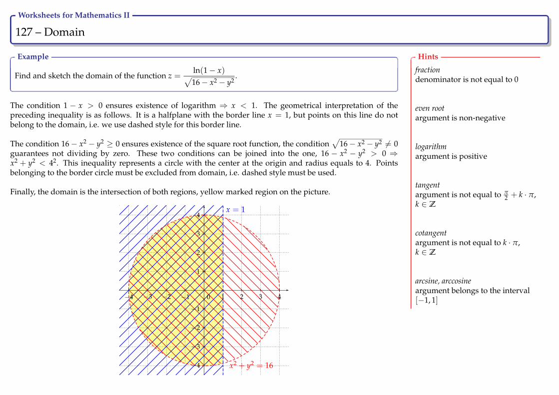
Worksheets for Mathematics II
127 – Domain Ry
Example
Find and sketch the domain of the function z =ln(1− x)√16− x2 − y2
.
The condition 1 − x > 0 ensures existence of logarithm ⇒ x < 1. The geometrical interpretation of thepreceding inequality is as follows. It is a halfplane with the border line x = 1, but points on this line do notbelong to the domain, i.e. we use dashed style for this border line.
The condition 16− x2 − y2 ≥ 0 ensures existence of the square root function, the condition√
16− x2 − y2 6= 0guarantees not dividing by zero. These two conditions can be joined into the one, 16 − x2 − y2 > 0 ⇒x2 + y2 < 42. This inequality represents a circle with the center at the origin and radius equals to 4. Pointsbelonging to the border circle must be excluded from domain, i.e. dashed style must be used.
Finally, the domain is the intersection of both regions, yellow marked region on the picture.
x = 1
x2 + y2 = 16
−4 −3 −2 −1 1 2 3 4
−4
−3
−2
−1
1
2
3
4
0
Hints
fractiondenominator is not equal to 0
even rootargument is non-negative
logarithmargument is positive
tangentargument is not equal to π
2 + k · π,k ∈ Z
cotangentargument is not equal to k · π,k ∈ Z
arcsine, arccosineargument belongs to the interval[−1, 1]
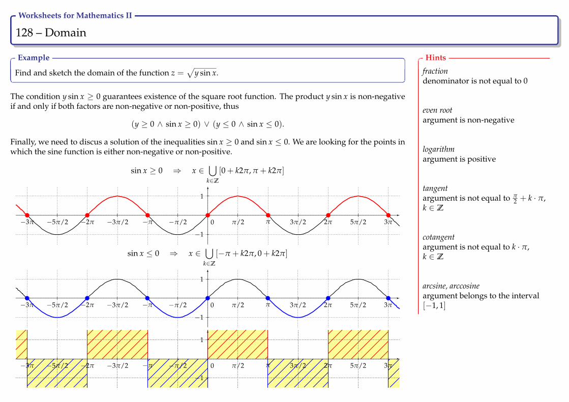
Worksheets for Mathematics II
128 – Domain Ry
Example
Find and sketch the domain of the function z =√
y sin x.
The condition y sin x ≥ 0 guarantees existence of the square root function. The product y sin x is non-negativeif and only if both factors are non-negative or non-positive, thus
(y ≥ 0 ∧ sin x ≥ 0) ∨ (y ≤ 0 ∧ sin x ≤ 0).
Finally, we need to discus a solution of the inequalities sin x ≥ 0 and sin x ≤ 0. We are looking for the points inwhich the sine function is either non-negative or non-positive.
sin x ≥ 0 ⇒ x ∈⋃
k∈Z
[0 + k2π, π + k2π]
−1
1
0−3π −5π/2 −2π −3π/2 −π −π/2 3π5π/22π3π/2ππ/2
sin x ≤ 0 ⇒ x ∈⋃
k∈Z
[−π + k2π, 0 + k2π]
−1
1
0−3π −5π/2 −2π −3π/2 −π −π/2 3π5π/22π3π/2ππ/2
−1
1
0−3π −5π/2 −2π −3π/2 −π −π/2 3π5π/22π3π/2ππ/2
Hints
fractiondenominator is not equal to 0
even rootargument is non-negative
logarithmargument is positive
tangentargument is not equal to π
2 + k · π,k ∈ Z
cotangentargument is not equal to k · π,k ∈ Z
arcsine, arccosineargument belongs to the interval[−1, 1]

Worksheets for Mathematics II
129 – Domain Ry
Exercise
Find the domain of the function:
a) z =x− y + 8x + y− 2
b) z =√
2x + y
−5 −4 −3 −2 −1 1 2 3 4
−5
−4
−3
−2
−1
1
2
3
4
0 −5 −4 −3 −2 −1 1 2 3 4
−5
−4
−3
−2
−1
1
2
3
4
0
Hints
fractiondenominator is not equal to 0
even rootargument is non-negative
logarithmargument is positive
tangentargument is not equal to π
2 + k · π,k ∈ Z
cotangentargument is not equal to k · π,k ∈ Z
arcsine, arccosineargument belongs to the interval[−1, 1]

Worksheets for Mathematics II
130 – Domain Ry
Exercise
Find the domain of the function:
a) z =√
y2 − 1 b) z =x + 2y√
y2 − 4+√
x2 − 1
−5 −4 −3 −2 −1 1 2 3 4
−5
−4
−3
−2
−1
1
2
3
4
0 −5 −4 −3 −2 −1 1 2 3 4
−5
−4
−3
−2
−1
1
2
3
4
0
Hints
fractiondenominator is not equal to 0
even rootargument is non-negative
logarithmargument is positive
tangentargument is not equal to π
2 + k · π,k ∈ Z
cotangentargument is not equal to k · π,k ∈ Z
arcsine, arccosineargument belongs to the interval[−1, 1]
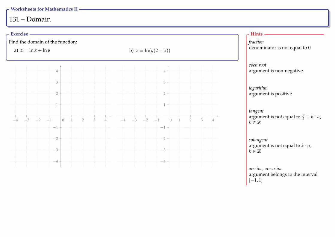
Worksheets for Mathematics II
131 – Domain Ry
Exercise
Find the domain of the function:
a) z = ln x + ln y b) z = ln(y(2− x))
−5 −4 −3 −2 −1 1 2 3 4
−5
−4
−3
−2
−1
1
2
3
4
0 −5 −4 −3 −2 −1 1 2 3 4
−5
−4
−3
−2
−1
1
2
3
4
0
Hints
fractiondenominator is not equal to 0
even rootargument is non-negative
logarithmargument is positive
tangentargument is not equal to π
2 + k · π,k ∈ Z
cotangentargument is not equal to k · π,k ∈ Z
arcsine, arccosineargument belongs to the interval[−1, 1]

Worksheets for Mathematics II
132 – Domain Ry
Exercise
Find the domain of the function:
a) z =√
16− x2 − y2b) z =
1arcsin x arccos 2y
−5 −4 −3 −2 −1 1 2 3 4
−5
−4
−3
−2
−1
1
2
3
4
0 −5 −4 −3 −2 −1 1 2 3 4
−5
−4
−3
−2
−1
1
2
3
4
0
Hints
fractiondenominator is not equal to 0
even rootargument is non-negative
logarithmargument is positive
tangentargument is not equal to π
2 + k · π,k ∈ Z
cotangentargument is not equal to k · π,k ∈ Z
arcsine, arccosineargument belongs to the interval[−1, 1]

Worksheets for Mathematics II
133 – Domain Ry
Exercise
Find the domain of the function:
a) z = ln(xy− 4) b) z =
√y− x2
x3 − y
−5 −4 −3 −2 −1 1 2 3 4
−5
−4
−3
−2
−1
1
2
3
4
0 −5 −4 −3 −2 −1 1 2 3 4
−5
−4
−3
−2
−1
1
2
3
4
0
Hints
fractiondenominator is not equal to 0
even rootargument is non-negative
logarithmargument is positive
tangentargument is not equal to π
2 + k · π,k ∈ Z
cotangentargument is not equal to k · π,k ∈ Z
arcsine, arccosineargument belongs to the interval[−1, 1]
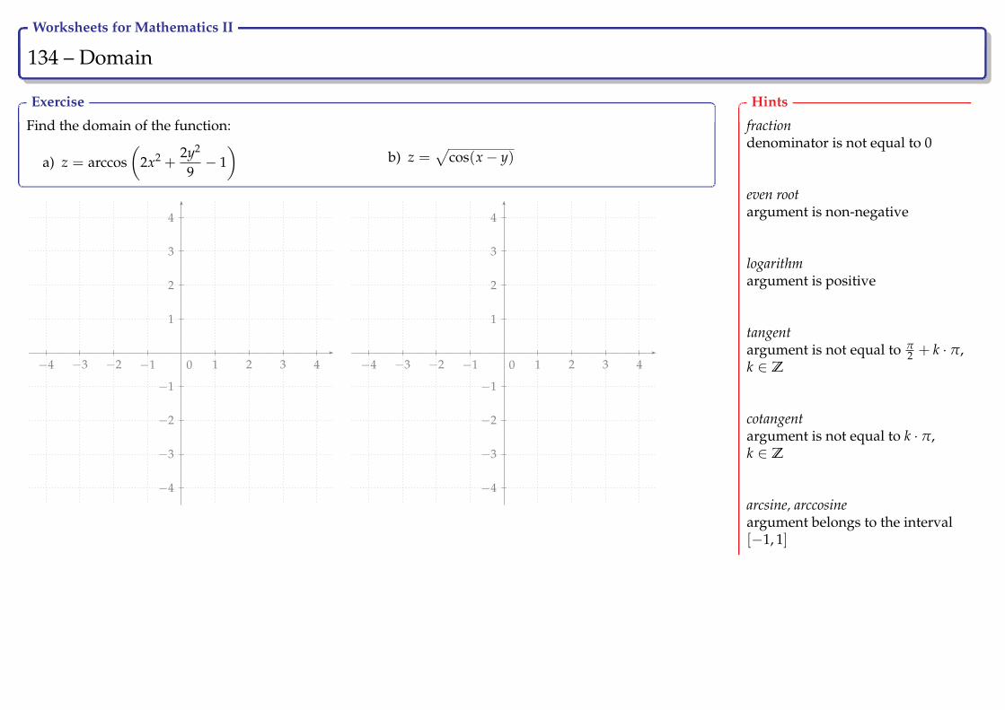
Worksheets for Mathematics II
134 – Domain Ry
Exercise
Find the domain of the function:
a) z = arccos(
2x2 +2y2
9− 1)
b) z =√
cos(x− y)
−5 −4 −3 −2 −1 1 2 3 4
−5
−4
−3
−2
−1
1
2
3
4
0 −5 −4 −3 −2 −1 1 2 3 4
−5
−4
−3
−2
−1
1
2
3
4
0
Hints
fractiondenominator is not equal to 0
even rootargument is non-negative
logarithmargument is positive
tangentargument is not equal to π
2 + k · π,k ∈ Z
cotangentargument is not equal to k · π,k ∈ Z
arcsine, arccosineargument belongs to the interval[−1, 1]

Worksheets for Mathematics II
135 – Domain Ry
Exercise
Decide which domain corresponds to the function z = arcsinx2 + y2 − 5
4.
−5 −4 −3 −2 −1 1 2 3 4
−5
−4
−3
−2
−1
1
2
3
4
0
¬
−5 −4 −3 −2 −1 1 2 3 4
−5
−4
−3
−2
−1
1
2
3
4
0
−5 −4 −3 −2 −1 1 2 3 4
−5
−4
−3
−2
−1
1
2
3
4
0
®
Hints
fractiondenominator is not equal to 0
even rootargument is non-negative
logarithmargument is positive
tangentargument is not equal to π
2 + k · π,k ∈ Z
cotangentargument is not equal to k · π,k ∈ Z
arcsine, arccosineargument belongs to the interval[−1, 1]
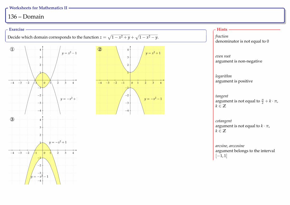
Worksheets for Mathematics II
136 – Domain Ry
Exercise
Decide which domain corresponds to the function z =√
1− x2 + y +√
1− x2 − y.
y = x2 − 1
y = −x2 + 1
−5 −4 −3 −2 −1 1 2 3 4
−5
−4
−3
−2
−1
1
2
3
4
0
¬y = x2 + 1
y = −x2 − 1
−5 −4 −3 −2 −1 1 2 3 4
−5
−4
−3
−2
−1
1
2
3
4
0
y = −x2 + 1
y = −x2 − 1
−5 −4 −3 −2 −1 1 2 3 4
−5
−4
−3
−2
−1
1
2
3
4
0
®
Hints
fractiondenominator is not equal to 0
even rootargument is non-negative
logarithmargument is positive
tangentargument is not equal to π
2 + k · π,k ∈ Z
cotangentargument is not equal to k · π,k ∈ Z
arcsine, arccosineargument belongs to the interval[−1, 1]
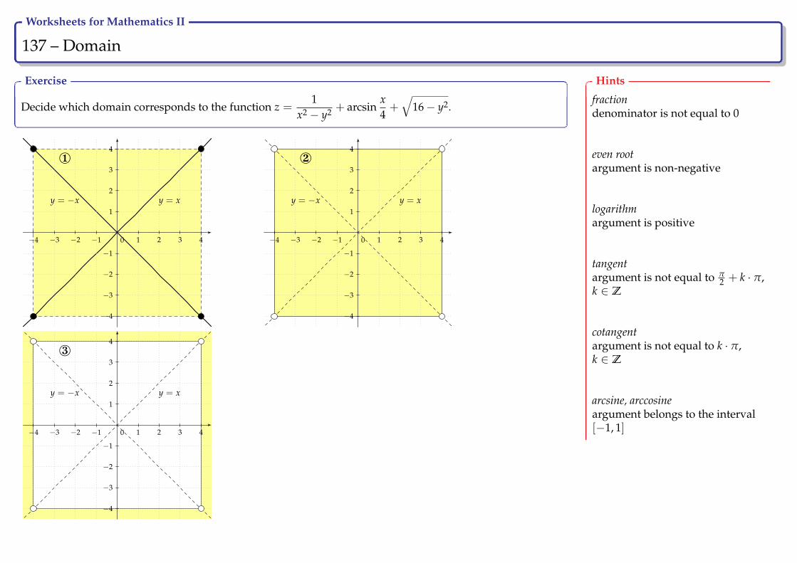
Worksheets for Mathematics II
137 – Domain Ry
Exercise
Decide which domain corresponds to the function z =1
x2 − y2 + arcsinx4+√
16− y2.
y = xy = −x
−5 −4 −3 −2 −1 1 2 3 4
−5
−4
−3
−2
−1
1
2
3
4
0
¬
y = xy = −x
−5 −4 −3 −2 −1 1 2 3 4
−5
−4
−3
−2
−1
1
2
3
4
0
y = xy = −x
−5 −4 −3 −2 −1 1 2 3 4
−5
−4
−3
−2
−1
1
2
3
4
0
®
Hints
fractiondenominator is not equal to 0
even rootargument is non-negative
logarithmargument is positive
tangentargument is not equal to π
2 + k · π,k ∈ Z
cotangentargument is not equal to k · π,k ∈ Z
arcsine, arccosineargument belongs to the interval[−1, 1]
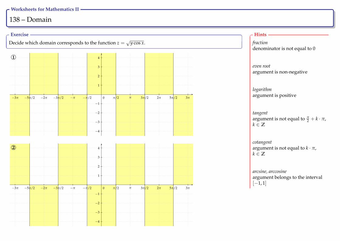
Worksheets for Mathematics II
138 – Domain Ry
Exercise
Decide which domain corresponds to the function z =√
y cos x.
−5
−4
−3
−2
−1
1
2
3
4
0−3π −5π/2 −2π −3π/2 −π −π/2 3π5π/22π3π/2ππ/2
¬
−5
−4
−3
−2
−1
1
2
3
4
0−3π −5π/2 −2π −3π/2 −π −π/2 3π5π/22π3π/2ππ/2
Hints
fractiondenominator is not equal to 0
even rootargument is non-negative
logarithmargument is positive
tangentargument is not equal to π
2 + k · π,k ∈ Z
cotangentargument is not equal to k · π,k ∈ Z
arcsine, arccosineargument belongs to the interval[−1, 1]

Worksheets for Mathematics II
139 – Functions of two real variables, graphs Ry
Definition
Graph of a function of two real variables is the set
G f = [x, y, z] ∈ R3 | [x, y] ∈ D f , z = f (x, y).
Remark
• The set G f is a subset in R3, G f ⊂ R3. Most often we work withsuch functions that their graphs are represented by 2-dimensionalsurfaces in 3-dimensional space.
• To draw the graph of a function “manually” is difficult in generaland mostly it cannot be done. One crucial option for the visual-ization of graphs is to use intersection curves of the given graphwith coordinate planes and their parallel planes, especially withxy-plane.
• For the visualization of graphs one can use computers and appro-priate software (GeoGebra, Gnuplot, Maple, Matlab, WolframAl-pha etc.).
• The graph of a function depending on three variables is repre-sented by the surface in 4-dimensional space R4, called hypersur-face. Such graph cannot be in our 3-dimensional space visualized.

Worksheets for Mathematics II
140 – Contour lines Ry
Definition
Sections of the graph of a function z = f (x, y) and planes parallel withthe coordinate xy-plane are called contours or contour lines. By con-tour graph we shall mean the projection of the contour lines into thexy-plane z = 0.
A contour line is a set of points belonging to the graph of a functionwith the same value. One can meat contours especially on touristicmaps (usually gray curves), where they represent the points with thesame altitude. On the picture one can see surroundings of VSB-TUO.
Contour plot and the graph of the function z =5x
x2 + y2 + 1.
−4 −3 −2 −1 1 2 3
k = 0
k = ±52
k = ±54
k = ±56
k = ±58
−4
−3
−2
−1
1
2
3
0
-4-3-2-101234
-4-3
-2-1
01
23
4
-3
-2
-1
0
1
2
3
z
x
y
z
-2.5-2-1.5-1-0.500.511.522.5

Worksheets for Mathematics II
141 – Contour lines Ry
Example
Find contour lines (contour plot) of the graph of the function z =5x
x2 + y2 + 1.
We substitute z = k, where k ∈ R.
1. For k = 0 (intersection of the graph with xy-plane) we get 0 =5x
x2 + y2 + 1⇒ x = 0, the contour
line is precisely y-axis.
2. For k 6= 0 we get
k =5x
x2 + y2 + 1⇒ x2 + y2 + 1 =
5xk
⇒ x2 − 5xk
+ y2 + 1 = 0 ⇒(
x− 52k
)2
+ y2 =254k2 − 1.
The contour lines are circles but only in the case, where right-hand side of the equation is positive,
254k2 − 1 > 0 ⇒ 25
4k2 > 1 ⇒ 25 > 4k2 ⇒ k2 <254
⇒ |k| < 52⇒ k ∈
(−5
2, 0)∪(
0,52
).
3. For k = ±52
holds (x∓ 1)2 + y2 = 0. We get as contours two singular circles, points [1, 0] and [−1, 0].
−4 −3 −2 −1 1 2 3
k = 0
k = ±52
k = ±54
k = ±56
k = ±58
−4
−3
−2
−1
1
2
3
0
-4-3-2-101234
-4-3
-2-1
01
23
4
-3
-2
-1
0
1
2
3
z
x
y
z
-2.5-2-1.5-1-0.500.511.522.5
Hints
We seek intersections of the graphwith planes parallel with xy-plane, i.e. z = k, k ∈ R.The number k is arbitrary but itmay happen that the intersectioncurve does not exist.
List of commands - Gnuplot:set view 62,210; set view equal xyset iso 50; set samp 50set xrange [-4:4]; set yrange [-4:4]set ztics 1; set pm3dset contour bothset cntrparam levels discrete 0, 2.485,-2.485, 1.25, -1.25, .83, -.83, .625, -.625set style increment userset style line 1 lc rgb ’black’ lw 2set style line 2 lc rgb ’red’set style line 3 lc rgb ’red’set style line 4 lc rgb ’yellow’set style line 5 lc rgb ’yellow’set style line 6 lc rgb ’green’set style line 7 lc rgb ’green’set style line 8 lc rgb ’cyan’set style line 9 lc rgb ’cyan’set style line 10 lc rgb ’magenta’set grid; unset surf; unset keyset xlabel "x"set ylabel "y"set zlabel "z"splot 5*x/(x**2+y**2+1)
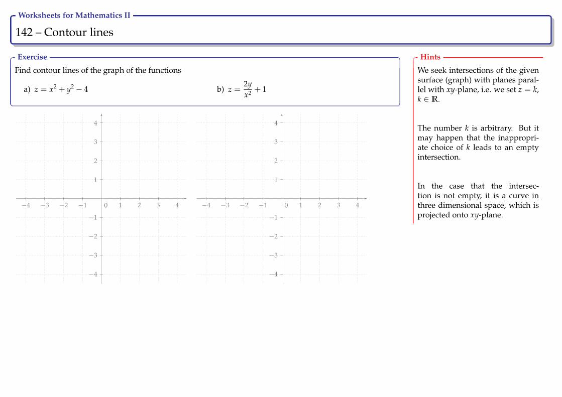
Worksheets for Mathematics II
142 – Contour lines Ry
Exercise
Find contour lines of the graph of the functions
a) z = x2 + y2 − 4 b) z =2yx2 + 1
−5 −4 −3 −2 −1 1 2 3 4
−5
−4
−3
−2
−1
1
2
3
4
0 −5 −4 −3 −2 −1 1 2 3 4
−5
−4
−3
−2
−1
1
2
3
4
0
Hints
We seek intersections of the givensurface (graph) with planes paral-lel with xy-plane, i.e. we set z = k,k ∈ R.
The number k is arbitrary. But itmay happen that the inappropri-ate choice of k leads to an emptyintersection.
In the case that the intersec-tion is not empty, it is a curve inthree dimensional space, which isprojected onto xy-plane.

Worksheets for Mathematics II
143 – Contour lines Ry
Exercise
Decide which contour plot corresponds to the function z = x2y2.
y =
√k
x, k > 0
0
¬
y = −√
kx
, k > 0
0
0
®
k = 0k = 1k = 9k = 25k = 49
Hints
We seek intersections of the givensurface (graph) with planes paral-lel with xy-plane, i.e. we set z = k,k ∈ R.
The number k is arbitrary. But itmay happen that the inappropri-ate choice of k leads to an emptyintersection.
In the case that the intersec-tion is not empty, it is a curve inthree dimensional space, whichis projected onto xy-plane to getcontour plot.
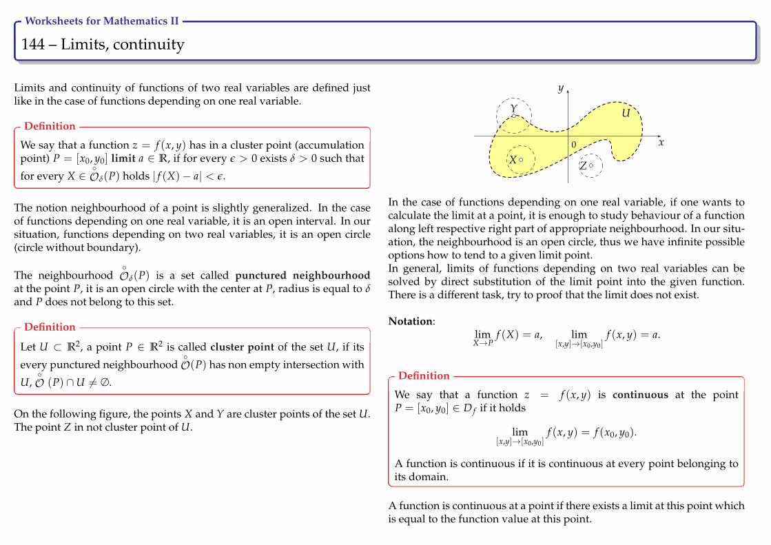
Worksheets for Mathematics II
144 – Limits, continuity Ry
Limits and continuity of functions of two real variables are defined justlike in the case of functions depending on one real variable.
Definition
We say that a function z = f (x, y) has in a cluster point (accumulationpoint) P = [x0, y0] limit a ∈ R, if for every ε > 0 exists δ > 0 such that
for every X ∈Oδ(P) holds | f (X)− a| < ε.
The notion neighbourhood of a point is slightly generalized. In the caseof functions depending on one real variable, it is an open interval. In oursituation, functions depending on two real variables, it is an open circle(circle without boundary).
The neighbourhoodOδ(P) is a set called punctured neighbourhood
at the point P, it is an open circle with the center at P, radius is equal to δand P does not belong to this set.
Definition
Let U ⊂ R2, a point P ∈ R2 is called cluster point of the set U, if its
every punctured neighbourhoodO(P) has non empty intersection with
U,O (P) ∩U 6= ∅.
On the following figure, the points X and Y are cluster points of the set U.The point Z in not cluster point of U.
x
y
0
U
X
Y
Z
In the case of functions depending on one real variable, if one wants tocalculate the limit at a point, it is enough to study behaviour of a functionalong left respective right part of appropriate neighbourhood. In our situ-ation, the neighbourhood is an open circle, thus we have infinite possibleoptions how to tend to a given limit point.In general, limits of functions depending on two real variables can besolved by direct substitution of the limit point into the given function.There is a different task, try to proof that the limit does not exist.
Notation:limX→P
f (X) = a, lim[x,y]→[x0,y0]
f (x, y) = a.
Definition
We say that a function z = f (x, y) is continuous at the pointP = [x0, y0] ∈ D f if it holds
lim[x,y]→[x0,y0]
f (x, y) = f (x0, y0).
A function is continuous if it is continuous at every point belonging toits domain.
A function is continuous at a point if there exists a limit at this point whichis equal to the function value at this point.
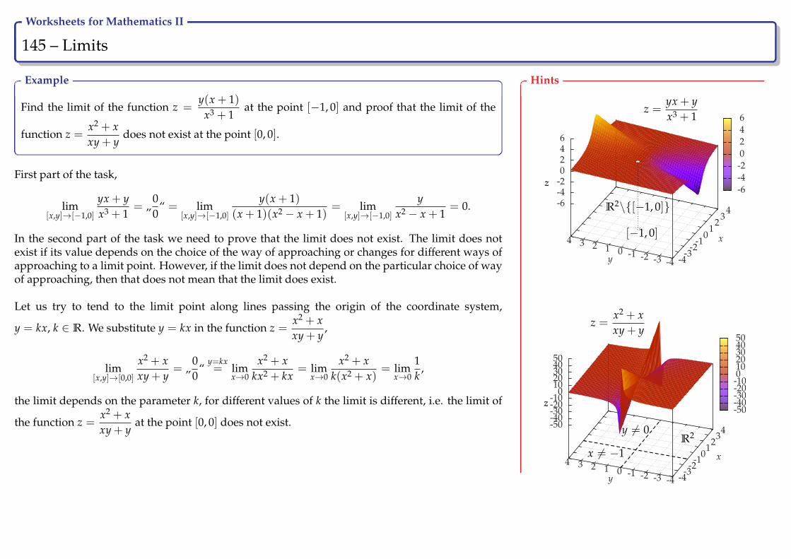
Worksheets for Mathematics II
145 – Limits Ry
Example
Find the limit of the function z =y(x + 1)
x3 + 1at the point [−1, 0] and proof that the limit of the
function z =x2 + xxy + y
does not exist at the point [0, 0].
First part of the task,
lim[x,y]→[−1,0]
yx + yx3 + 1
= „00
“ = lim[x,y]→[−1,0]
y(x + 1)(x + 1)(x2 − x + 1)
= lim[x,y]→[−1,0]
yx2 − x + 1
= 0.
In the second part of the task we need to prove that the limit does not exist. The limit does notexist if its value depends on the choice of the way of approaching or changes for different ways ofapproaching to a limit point. However, if the limit does not depend on the particular choice of wayof approaching, then that does not mean that the limit does exist.
Let us try to tend to the limit point along lines passing the origin of the coordinate system,
y = kx, k ∈ R. We substitute y = kx in the function z =x2 + xxy + y
,
lim[x,y]→[0,0]
x2 + xxy + y
= „00
“y=kx= lim
x→0
x2 + xkx2 + kx
= limx→0
x2 + xk(x2 + x)
= limx→0
1k
,
the limit depends on the parameter k, for different values of k the limit is different, i.e. the limit of
the function z =x2 + xxy + y
at the point [0, 0] does not exist.
Hints
-4-3
-2-1
01
23
4
-4-3-2-101234
-6
-4
-2
0
2
4
6
z
x
y
z-6
-4
-2
0
2
4
6z =
yx + yx3 + 1
[−1, 0]
R2\[−1, 0]
z =x2 + xxy + y
-4-3
-2-1
01
23
4
-4-3-2-101234
-50-40-30-20-10
01020304050
z
x
y
z-50-40-30-20-1001020304050
y 6= 0
x 6= −1R2

Worksheets for Mathematics II
146 – Limits Ry
Exercise
Solve,
a) lim[x,y]→[1,2]
xy + x− yx3 − 2
b) lim[x,y]→[π
2 ,− 5π6 ]
sin(2x + y) c) lim[x,y]→[−1,4]
x3 + 1y(x + 1)
Hints
Limits of functions of two realvariables are mostly solved bymeans of direct substitution of thelimit points or by some manipula-tions with the functions.
On the other side, quite fre-quent task it to proof that the limitdoes not exist.

Worksheets for Mathematics II
147 – Partial derivatives Ry
Definition
We say that a function z = f (x, y) has partial derivative with respect tox (of the first order) at the point A = [x0, y0], if there exists proper limit
∂ f∂x
(A) = limh→0
f (x0 + h, y0)− f (x0, y0)
h.
Analogously, one can define partial derivative with respect to y,
∂ f∂y
(A) = limh→0
f (x0, y0 + h)− f (x0, y0)
h.
Remark
• Notation:∂ f∂x
(A),∂z∂x
(A), fx(A), f ′x(A), etc.
• Partial derivatives∂ f∂x
respective∂ f∂y
are again functions depend-
ing on two real variables.
• Partial derivatives of functions depending on three and more realvariables can be defined analogously.
• When we calculate partial derivative with respect to x, we keep yfixed and treat it as a constant, i.e. such function is differentiatedlike the function depending only on one real variable. For partialderivatives with respect to y we proceed in the same way, we keepx fixed.
In fact, the calculation of partial derivatives of functions depending ontwo real variable reduces to the calculation of derivatives of functions de-pending on one real variable. One can use the same formulas and rules fordifferentiation of functions depending on one real variable.
Theorem
Let there exist partial derivatives of functions f (x, y) and g(x, y) withrespect to x = x1 and y = x2 on Q ⊆ D f ∩ Dg at the point X. Then forevery i = 1, 2 holds,
∂
∂xi( f ± g)(X) =
∂ f∂xi
(X)± ∂g∂xi
(X),
∂
∂xi( f · g)(X) =
∂ f∂xi
(X) · g(X) + f (X) · ∂g∂xi
(X),
∂
∂xi
(fg
)(X) =
∂ f∂xi
(X) · g(X)− f (X) · ∂g∂xi
(X)
g2(X).
Definition
Partial derivatives of the second order of a function z = f (x, y) aredefined as follows,
∂2 f∂x2 =
∂
∂x
(∂ f∂x
),
∂2 f∂y2 =
∂
∂y
(∂ f∂y
),
∂2 f∂x∂y
=∂
∂y
(∂ f∂x
),
∂2 f∂y∂x
=∂
∂x
(∂ f∂y
).
The following Schwarz theorem describes important property of mixedpartial derivatives.
Theorem (Schwarz)
If mixed partial derivatives∂2 f
∂x∂y,
∂2 f∂y∂x
are continuous at the point
A = [x0, y0], then they are at this point equal,∂2 f
∂x∂y(A) =
∂2 f∂y∂x
(A).
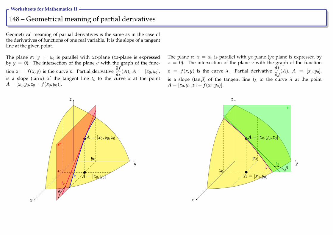
Worksheets for Mathematics II
148 – Geometrical meaning of partial derivatives Ry
Geometrical meaning of partial derivatives is the same as in the case ofthe derivatives of functions of one real variable. It is the slope of a tangentline at the given point.
The plane σ: y = y0 is parallel with xz-plane (xz-plane is expressedby y = 0). The intersection of the plane σ with the graph of the func-
tion z = f (x, y) is the curve κ. Partial derivative∂ f∂x
(A), A = [x0, y0],is a slope (tan α) of the tangent line tκ to the curve κ at the pointA = [x0, y0, z0 = f (x0, y0)].
y
z
x
A = [x0, y0]
y0
x0
tκ
κ
A = [x0, y0, z0]
α
σ
The plane ν: x = x0 is parallel with yz-plane (yz-plane is expressed byx = 0). The intersection of the plane ν with the graph of the function
z = f (x, y) is the curve λ. Partial derivative∂ f∂y
(A), A = [x0, y0],
is a slope (tan β) of the tangent line tλ to the curve λ at the pointA = [x0, y0, z0 = f (x0, y0)].
y
z
x
A = [x0, y0]
y0
x0
tλλ
A = [x0, y0, z0]
β
ν

Worksheets for Mathematics II
149 – Partial derivatives of the first order Ry
Example
Find partial derivatives of the first order of the function z = x2 sin2(xy2) at the point [π, 0].
We calculate partial derivatives with respect to all independent variables, i.e. with respect to x and y. If we fixone independent variable, e.g. y, such variable is considered as a constant c, the function z = f (x, y) becomesthe function depending on one real variable z = f (x, c), and can be easily differentiated with the help offormulas in the hint list.
Partial derivative∂z∂x
of the function z with respect to x:
because the function z is differentiated with respect to x, the variable y is considered as a constant. Ourtask is to differentiate multiplication of two functions depending on x, the function x2 and the composedfunction sin2(xy2), which must be differentiated in the following order of components: second power, sinefunction, xy2; in the expression xy2 is y2 a constant factor, therefore we have to differentiate only x,
∂z∂x
=∂
∂x(x2) · sin2(xy2) + x2 · ∂
∂x(sin2(xy2))
= 2x sin2(xy2) + x2 · 2 sin(xy2) · cos(xy2) · y2 = 2x sin2(xy2) + 2x2y2 sin(xy2) cos(xy2).
Partial derivative∂z∂y
of the function z with respect to y:
differentiation is analogous, as a constant we mean x variable, again we differentiate a composed func-tion; x2 is a constant factor, i.e. only second factor must be differentiated with respect to y as a composedfunction with the following order of components: second root, sine function, xy2; in the expression xy2 is xconsidered as a constant factor, thus we differentiate only y2,
∂z∂y
= x2 · ∂z∂y
(sin2(xy2)) = x2 · 2 sin(xy2) · cos(xy2) · x2y = 4x3y sin(xy2) cos(xy2).
Partial derivatives are again functions depending on two real variables and can be easily evaluated at the givenpoint by direct substitution:
∂z∂x
(π, 0) = 0,∂z∂y
(π, 0) = 0.
Hints
1. (c)′ = 0
2. (xn)′ = nxn−1
3. (ex)′ = ex
4. (ax)′ = ax ln a
5. (ln x)′ =1x
6. (loga x)′ =1
x ln a7. (sin x)′ = cos x
8. (cos x)′ = − sin x
9. (tan x)′ =1
cos2 x10. (cot x)′ = − 1
sin2 x11. (arcsin x)′ =
1√1− x2
12. (arccos x)′ = − 1√1− x2
13. (arctan x)′ =1
1 + x2
14. (arccot x)′ = − 11 + x2
15. [c · u]′ = c · u′, c ∈ R
16. [u± v]′ = u′ ± v′
17. [u · v]′ = u′ · v + u · v′
18.[u
v
]′=
u′ · v− u · v′v2
19. [u(v)]′ = u′(v) · v′

Worksheets for Mathematics II
150 – Partial derivatives of the first order Ry
Exercise
Find partial derivatives of the first order:
a) z = x2 + y2
b) z = sin(2x + y)
c) z = (x3 + 1)y(x + 1)
d) z =xy + x− y
x3 − 2
e) z =
√xy
ln(x− y2)
f) z = tan(ln(xy))
Hints
1. (c)′ = 0
2. (xn)′ = nxn−1
3. (ex)′ = ex
4. (ax)′ = ax ln a
5. (ln x)′ =1x
6. (loga x)′ =1
x ln a7. (sin x)′ = cos x
8. (cos x)′ = − sin x
9. (tan x)′ =1
cos2 x10. (cot x)′ = − 1
sin2 x11. (arcsin x)′ =
1√1− x2
12. (arccos x)′ = − 1√1− x2
13. (arctan x)′ =1
1 + x2
14. (arccot x)′ = − 11 + x2
15. [c · u]′ = c · u′, c ∈ R
16. [u± v]′ = u′ ± v′
17. [u · v]′ = u′ · v + u · v′
18.[u
v
]′=
u′ · v− u · v′v2
19. [u(v)]′ = u′(v) · v′
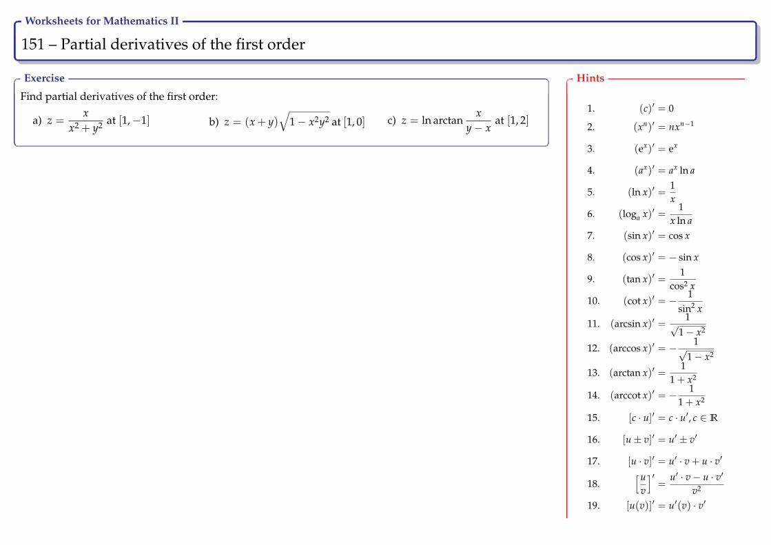
Worksheets for Mathematics II
151 – Partial derivatives of the first order Ry
Exercise
Find partial derivatives of the first order:
a) z =x
x2 + y2 at [1,−1] b) z = (x+ y)√
1− x2y2 at [1, 0] c) z = ln arctanx
y− xat [1, 2]
Hints
1. (c)′ = 0
2. (xn)′ = nxn−1
3. (ex)′ = ex
4. (ax)′ = ax ln a
5. (ln x)′ =1x
6. (loga x)′ =1
x ln a7. (sin x)′ = cos x
8. (cos x)′ = − sin x
9. (tan x)′ =1
cos2 x10. (cot x)′ = − 1
sin2 x11. (arcsin x)′ =
1√1− x2
12. (arccos x)′ = − 1√1− x2
13. (arctan x)′ =1
1 + x2
14. (arccot x)′ = − 11 + x2
15. [c · u]′ = c · u′, c ∈ R
16. [u± v]′ = u′ ± v′
17. [u · v]′ = u′ · v + u · v′
18.[u
v
]′=
u′ · v− u · v′v2
19. [u(v)]′ = u′(v) · v′

Worksheets for Mathematics II
152 – Partial derivatives of the second order Ry
Example
Find partial derivatives of the second order of the function z = xy at the point [1, 1].
At first, we need to calculate partial derivatives of the first order,
In the derivative with respect to x, we differentiate power function, formula 2∂z∂x
= yxy−1
In the derivative with respect to y, we differentiate exponential function, formula 4∂z∂y
= xy ln x
To find partial derivatives of the second order, it is necessary to differentiate partial derivatives of the first orderwith respect to x and y,
∂2z∂x2 =
∂
∂x
(∂z∂x
)=
∂
∂x(yxy−1) = y(y− 1)xy−2,
∂2z∂x∂y
=∂
∂y
(∂z∂x
)=
∂
∂y(yxy−1) = xy−1 + yxy−1 ln x,
∂2z∂y∂x
=∂
∂x
(∂z∂y
)=
∂
∂x(xy ln x) = yxy−1 ln x + xy 1
x,
∂2z∂y2 =
∂
∂y
(∂z∂y
)=
∂
∂y(xy ln x) = xy ln x ln x = xy ln2 x.
Stress that in the case of continuous functions with continuous partial derivatives, the mixed derivatives arethe same according to Schwarz theorem. Indeed:
∂2z∂y∂x
= yxy−1 ln x + xy 1x= yxy−1 ln x + xyx−1 = yxy−1 ln x + xy−1 = xy−1 + yxy−1 ln x =
∂2z∂x∂y
.
Finally, the simple evaluation of partial derivatives of the second order at the point [1, 1] remains,
∂2z∂x2 (1, 1) = 0,
∂2z∂x∂y
(1, 1) = 1,∂2z
∂y∂x(1, 1) = 1,
∂2z∂y2 (1, 1) = 0.
Hints
1. (c)′ = 0
2. (xn)′ = nxn−1
3. (ex)′ = ex
4. (ax)′ = ax ln a
5. (ln x)′ =1x
6. (loga x)′ =1
x ln a7. (sin x)′ = cos x
8. (cos x)′ = − sin x
9. (tan x)′ =1
cos2 x10. (cot x)′ = − 1
sin2 x11. (arcsin x)′ =
1√1− x2
12. (arccos x)′ = − 1√1− x2
13. (arctan x)′ =1
1 + x2
14. (arccot x)′ = − 11 + x2
15. [c · u]′ = c · u′, c ∈ R
16. [u± v]′ = u′ ± v′
17. [u · v]′ = u′ · v + u · v′
18.[u
v
]′=
u′ · v− u · v′v2
19. [u(v)]′ = u′(v) · v′

Worksheets for Mathematics II
153 – Partial derivatives of the second order Ry
Exercise
Find partial derivatives of the second order:
a) z = cot(x + 2y) b) z = xe(y+1) c) z = xy
Hints
1. (c)′ = 0
2. (xn)′ = nxn−1
3. (ex)′ = ex
4. (ax)′ = ax ln a
5. (ln x)′ =1x
6. (loga x)′ =1
x ln a7. (sin x)′ = cos x
8. (cos x)′ = − sin x
9. (tan x)′ =1
cos2 x10. (cot x)′ = − 1
sin2 x11. (arcsin x)′ =
1√1− x2
12. (arccos x)′ = − 1√1− x2
13. (arctan x)′ =1
1 + x2
14. (arccot x)′ = − 11 + x2
15. [c · u]′ = c · u′, c ∈ R
16. [u± v]′ = u′ ± v′
17. [u · v]′ = u′ · v + u · v′
18.[u
v
]′=
u′ · v− u · v′v2
19. [u(v)]′ = u′(v) · v′
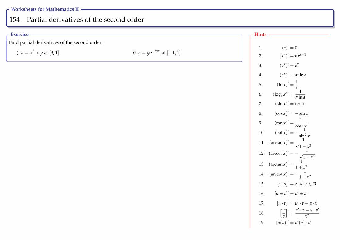
Worksheets for Mathematics II
154 – Partial derivatives of the second order Ry
Exercise
Find partial derivatives of the second order:
a) z = x2 ln y at [3, 1] b) z = ye−xy2at [−1, 1]
Hints
1. (c)′ = 0
2. (xn)′ = nxn−1
3. (ex)′ = ex
4. (ax)′ = ax ln a
5. (ln x)′ =1x
6. (loga x)′ =1
x ln a7. (sin x)′ = cos x
8. (cos x)′ = − sin x
9. (tan x)′ =1
cos2 x10. (cot x)′ = − 1
sin2 x11. (arcsin x)′ =
1√1− x2
12. (arccos x)′ = − 1√1− x2
13. (arctan x)′ =1
1 + x2
14. (arccot x)′ = − 11 + x2
15. [c · u]′ = c · u′, c ∈ R
16. [u± v]′ = u′ ± v′
17. [u · v]′ = u′ · v + u · v′
18.[u
v
]′=
u′ · v− u · v′v2
19. [u(v)]′ = u′(v) · v′

Worksheets for Mathematics II
155 – Partial derivative of the fourth order Ry
Example
Find partial derivative of the fourth order∂4z
∂x2∂y2 of the function z = 2x2ey + sin(xy2).
We differentiate the function z according to single variables. We start differentiation with respect to x, thenagain with respect to x and finally two times with respect to y.
∂z∂x
= 4xey + cos(xy2) · y2 = 4xey + y2 cos(xy2)
∂2z∂x2 = 4ey + y2(− sin(xy2) · y2) = 4ey − y4 sin(xy2)
∂3z∂x2∂y
= 4ey − [4y3 sin(xy2) + y4 cos(xy2) · x2y] = 4ey − 4y3 sin(xy2)− 2xy5 cos(xy2)
∂4z∂x2∂y2 = 4ey − [12y2 sin(xy2) + 4y3 cos(xy2) · x2y]− [10xy4 cos(xy2) + 2xy5(− sin(xy2) · x2y)]
= 4ey − 12y2 sin(xy2)− 8xy4 cos(xy2)− 10xy4 cos(xy2) + 4x2y6 sin(xy2)
= 4ey − 12y2 sin(xy2)− 18xy4 cos(xy2) + 4x2y6 sin(xy2)
Hints
1. (c)′ = 0
2. (xn)′ = nxn−1
3. (ex)′ = ex
4. (ax)′ = ax ln a
5. (ln x)′ =1x
6. (loga x)′ =1
x ln a7. (sin x)′ = cos x
8. (cos x)′ = − sin x
9. (tan x)′ =1
cos2 x10. (cot x)′ = − 1
sin2 x11. (arcsin x)′ =
1√1− x2
12. (arccos x)′ = − 1√1− x2
13. (arctan x)′ =1
1 + x2
14. (arccot x)′ = − 11 + x2
15. [c · u]′ = c · u′, c ∈ R
16. [u± v]′ = u′ ± v′
17. [u · v]′ = u′ · v + u · v′
18.[u
v
]′=
u′ · v− u · v′v2
19. [u(v)]′ = u′(v) · v′
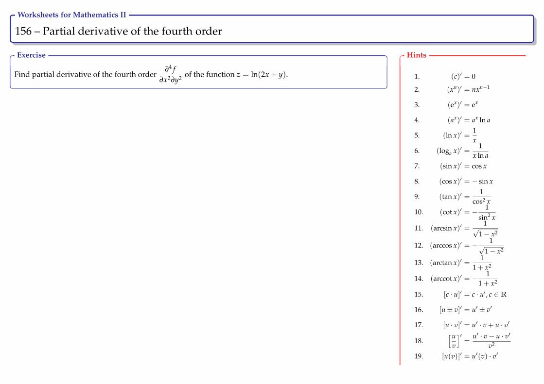
Worksheets for Mathematics II
156 – Partial derivative of the fourth order Ry
Exercise
Find partial derivative of the fourth order∂4 f
∂x2∂y2 of the function z = ln(2x + y).
Hints
1. (c)′ = 0
2. (xn)′ = nxn−1
3. (ex)′ = ex
4. (ax)′ = ax ln a
5. (ln x)′ =1x
6. (loga x)′ =1
x ln a7. (sin x)′ = cos x
8. (cos x)′ = − sin x
9. (tan x)′ =1
cos2 x10. (cot x)′ = − 1
sin2 x11. (arcsin x)′ =
1√1− x2
12. (arccos x)′ = − 1√1− x2
13. (arctan x)′ =1
1 + x2
14. (arccot x)′ = − 11 + x2
15. [c · u]′ = c · u′, c ∈ R
16. [u± v]′ = u′ ± v′
17. [u · v]′ = u′ · v + u · v′
18.[u
v
]′=
u′ · v− u · v′v2
19. [u(v)]′ = u′(v) · v′

Worksheets for Mathematics II
157 – Differentials Ry
Definition
We say that a function z = f (x, y) is differentiable at the point A =[x0, y0], or it has differential at a point, if its increment ∆z on the neigh-bourhood of the point A can be expressed as
∆z = f (x0 + h, y0 + k)− f (x0, y0) = Ah + Bk + ρ · τ(h, k),
whereA and B are constants, ρ =√
h2 + k2 and lim[h,k]→[0,0] τ(h, k) = 0.The function z = f (x, y) is called differentiable, if it is differentiable atevery point belonging to its domain.
Theorem
If a function z = f (x, y) is differentiable at the point A, then there existpartial derivatives of the first order at the point A and it holds
A =∂ f∂x
(A), B =∂ f∂y
(A).
Remark
The number h represents an increment on x-axis, k is an increment ony-axis and we usually denote those increments by h = dx respectivek = dy. For the increment on z-axis at point A with known values of dxand dy we get
∆z =∂ f∂x
(A)dx +∂ f∂y
(A)dy + ρ · τ(dx, dy).
Definition
If a function z = f (x, y) is differentiable, the expression
dz = d f (x, y) =∂ f∂x
dx +∂ f∂y
dy
is called differential of the function z = f (x, y).
Theorem
If a function z = f (x, y) is differentiable at the point A, then it is contin-uous at this point.
Theorem
If partial derivatives of the first order of a function z = f (x, y) are con-tinuous at A, then the function z = f (x, y) is differentiable (and thuscontinuous) at the point A.
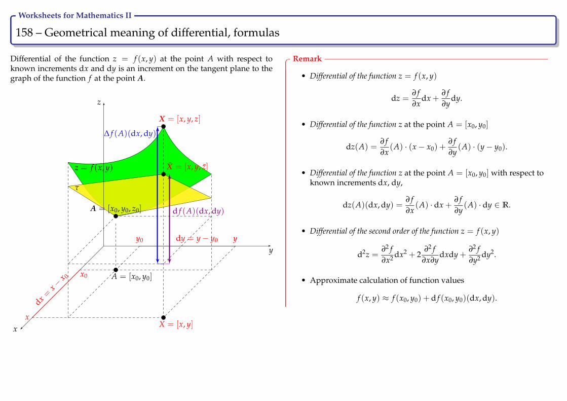
Worksheets for Mathematics II
158 – Geometrical meaning of differential, formulas Ry
Differential of the function z = f (x, y) at the point A with respect toknown increments dx and dy is an increment on the tangent plane to thegraph of the function f at the point A.
y
z
x
dx =x−
x 0
dy = y− y0
x
y
d f (A)(dx, dy)
∆ f (A)(dx, dy)
A = [x0, y0]
X = [x, y]
X = [x, y, z]
X = [x, y, z]
x0
y0
A = [x0, y0, z0]
τ
z = f (x, y)
Remark
• Differential of the function z = f (x, y)
dz =∂ f∂x
dx +∂ f∂y
dy.
• Differential of the function z at the point A = [x0, y0]
dz(A) =∂ f∂x
(A) · (x− x0) +∂ f∂y
(A) · (y− y0).
• Differential of the function z at the point A = [x0, y0] with respect toknown increments dx, dy,
dz(A)(dx, dy) =∂ f∂x
(A) · dx +∂ f∂y
(A) · dy ∈ R.
• Differential of the second order of the function z = f (x, y)
d2z =∂2 f∂x2 dx2 + 2
∂2 f∂x∂y
dxdy +∂2 f∂y2 dy2.
• Approximate calculation of function values
f (x, y) ≈ f (x0, y0) + d f (x0, y0)(dx, dy).

Worksheets for Mathematics II
159 – Differential of the first order Ry
Example
Find differential of the function z = f (x, y) =√
xy at the point A = [2, 1]. Calculate approxi-mately the function value f (2.04, 0.99).
At first, we calculate partial derivatives of the first order with respect to x and y,
∂ f∂x
=y
2√
xy,
∂ f∂y
=x
2√
xy.
For differential dz of the function z we have,
dz =y
2√
xydx +
x2√
xydy =
12√
xy(y dx + x dy).
We evaluate differential dz at the point A,
dz(A) = dz(2, 1) =1
2√
2(1(x− 2) + 2(y− 1)) =
√2
4(x + 2y− 4).
Note that differential at a point is a linear function depending on two real variables. For approxi-mate calculation of function values we need to find out increments from the point A = [2, 1] to thepoint [2.04, 0.99],
dx = x− x0 = 2.04− 2 = 0.04; dy = y− y0 = 0.99− 1 = −0.01.
We calculate the function value f (A) = f (2, 1) =√
2 and the value of differential dz(A)(dx, dy),
dz(A)(dx, dy) = dz(2, 1)(0.04,−0.01) =1
2√
2(1 · 0.04− 2 · 0.01) =
12√
20.02 =
12√
22
100=
√2
200.
The approximate function value f (2.04, 0.99) is
f (2.04, 0.99) ≈ f (A) + d f (A)(dx, dy) =√
2 +
√2
200=√
2(
1 +1
200
).
Hints
• Differential of the function z = f (x, y)
dz =∂ f∂x
dx +∂ f∂y
dy.
• Differential of the function z at the pointA = [x0, y0]
dz(A) =∂ f∂x
(A)(x− x0)+∂ f∂y
(A)(y− y0).
• Differential of the function z at the pointA = [x0, y0] with respect to known incre-ments dx, dy,
dz(A)(dx, dy) =∂ f∂x
(A)dx +∂ f∂y
(A)dy.
• Differential of the second order of the functionz = f (x, y)
d2z =∂2 f∂x2 dx2 + 2
∂2 f∂x∂y
dxdy +∂2 f∂y2 dy2.
• Approximate calculation of function val-ues
f (x, y) ≈ f (x0, y0) + d f (x0, y0)(dx, dy).
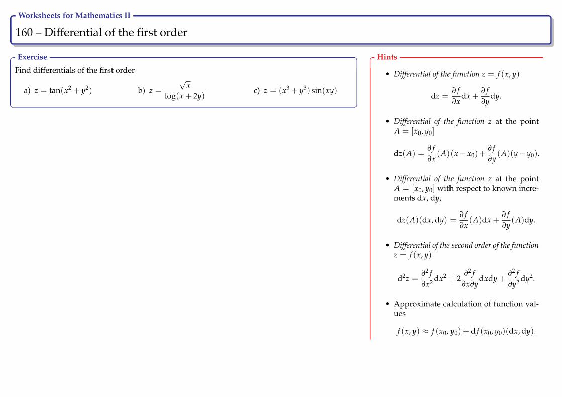
Worksheets for Mathematics II
160 – Differential of the first order Ry
Exercise
Find differentials of the first order
a) z = tan(x2 + y2) b) z =
√x
log(x + 2y)c) z = (x3 + y3) sin(xy)
Hints
• Differential of the function z = f (x, y)
dz =∂ f∂x
dx +∂ f∂y
dy.
• Differential of the function z at the pointA = [x0, y0]
dz(A) =∂ f∂x
(A)(x− x0)+∂ f∂y
(A)(y− y0).
• Differential of the function z at the pointA = [x0, y0] with respect to known incre-ments dx, dy,
dz(A)(dx, dy) =∂ f∂x
(A)dx +∂ f∂y
(A)dy.
• Differential of the second order of the functionz = f (x, y)
d2z =∂2 f∂x2 dx2 + 2
∂2 f∂x∂y
dxdy +∂2 f∂y2 dy2.
• Approximate calculation of function val-ues
f (x, y) ≈ f (x0, y0) + d f (x0, y0)(dx, dy).
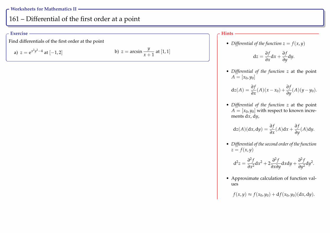
Worksheets for Mathematics II
161 – Differential of the first order at a point Ry
Exercise
Find differentials of the first order at the point
a) z = ex2y2−4 at [−1, 2] b) z = arcsiny
x + 1at [1, 1]
Hints
• Differential of the function z = f (x, y)
dz =∂ f∂x
dx +∂ f∂y
dy.
• Differential of the function z at the pointA = [x0, y0]
dz(A) =∂ f∂x
(A)(x− x0)+∂ f∂y
(A)(y− y0).
• Differential of the function z at the pointA = [x0, y0] with respect to known incre-ments dx, dy,
dz(A)(dx, dy) =∂ f∂x
(A)dx +∂ f∂y
(A)dy.
• Differential of the second order of the functionz = f (x, y)
d2z =∂2 f∂x2 dx2 + 2
∂2 f∂x∂y
dxdy +∂2 f∂y2 dy2.
• Approximate calculation of function val-ues
f (x, y) ≈ f (x0, y0) + d f (x0, y0)(dx, dy).
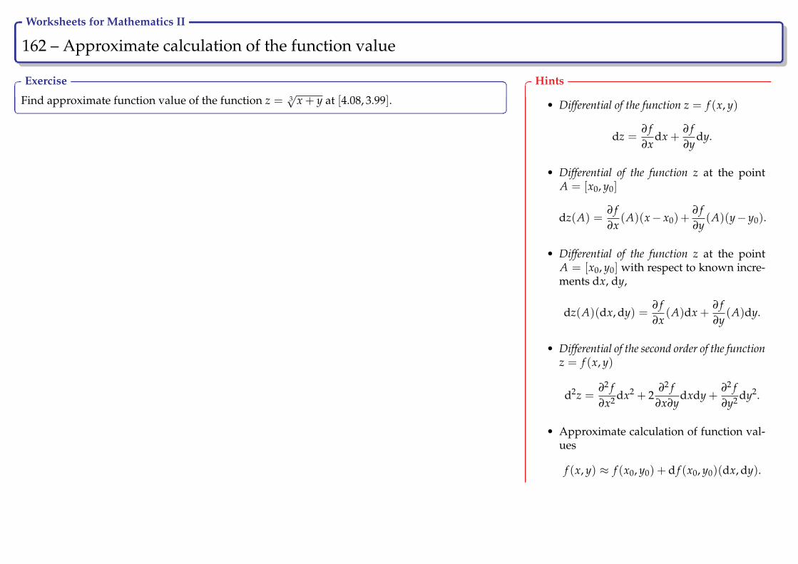
Worksheets for Mathematics II
162 – Approximate calculation of the function value Ry
Exercise
Find approximate function value of the function z = 3√
x + y at [4.08, 3.99].
Hints
• Differential of the function z = f (x, y)
dz =∂ f∂x
dx +∂ f∂y
dy.
• Differential of the function z at the pointA = [x0, y0]
dz(A) =∂ f∂x
(A)(x− x0)+∂ f∂y
(A)(y− y0).
• Differential of the function z at the pointA = [x0, y0] with respect to known incre-ments dx, dy,
dz(A)(dx, dy) =∂ f∂x
(A)dx +∂ f∂y
(A)dy.
• Differential of the second order of the functionz = f (x, y)
d2z =∂2 f∂x2 dx2 + 2
∂2 f∂x∂y
dxdy +∂2 f∂y2 dy2.
• Approximate calculation of function val-ues
f (x, y) ≈ f (x0, y0) + d f (x0, y0)(dx, dy).

Worksheets for Mathematics II
163 – Differential of the second order Ry
Example
Find differential of the second order of the function z = f (x, y) =x + yx− y
.
We calculate partial derivatives with respect to x and y,
∂ f∂x
=1 · (x− y)− (x + y) · 1
(x− y)2 =−2y
(x− y)2 ,
∂ f∂y
=1 · (x− y)− (x + y) · (−1)
(x− y)2 =2x
(x− y)2 .
We find out partial derivatives of the second order,
∂2 f∂x2 =
∂
∂x
(∂ f∂x
)=
∂
∂x(−2y(x− y)−2) = −2y(−2)(x− y)−3 · 1 =
4y(x− y)3 ,
∂2 f∂x∂y
=∂
∂y
(∂ f∂x
)=
∂
∂y
(−2y
(x− y)2
)=−2(x− y)2 − (−2y)2(x− y) · (−1)
(x− y)4 =−2(x + y)(x− y)3 ,
∂2 f∂y∂x
=∂
∂x
(∂ f∂y
)=
∂
∂x
(2x
(x− y)2
)=
2(x− y)2 − 2x · 2(x− y) · 1(x− y)4 =
−2(x + y)(x− y)3 ,
∂2 f∂y2 =
∂
∂y
(∂ f∂y
)=
∂
∂y(2x(x− y)−2) = 2x(−2)(x− y)−3 · (−1) =
4x(x− y)3 .
For differential of the second order we have
d2z =4y
(x− y)3 dx2 − 4x + y
(x− y)3 dxdy +4x
(x− y)3 dy2 =4
(x− y)3 (ydx2 − (x + y)dxdy + xdy2).
Hints
• Differential of the function z = f (x, y)
dz =∂ f∂x
dx +∂ f∂y
dy.
• Differential of the function z at the pointA = [x0, y0]
dz(A) =∂ f∂x
(A)(x− x0)+∂ f∂y
(A)(y− y0).
• Differential of the function z at the pointA = [x0, y0] with respect to known incre-ments dx, dy,
dz(A)(dx, dy) =∂ f∂x
(A)dx +∂ f∂y
(A)dy.
• Differential of the second order of the functionz = f (x, y)
d2z =∂2 f∂x2 dx2 + 2
∂2 f∂x∂y
dxdy +∂2 f∂y2 dy2.
• Approximate calculation of function val-ues
f (x, y) ≈ f (x0, y0) + d f (x0, y0)(dx, dy).

Worksheets for Mathematics II
164 – Differential of the second order Ry
Exercise
Find differentials of the second order
a) z =xy
x + yb) z = sin(5x + 2y)
Hints
• Differential of the function z = f (x, y)
dz =∂ f∂x
dx +∂ f∂y
dy.
• Differential of the function z at the pointA = [x0, y0]
dz(A) =∂ f∂x
(A)(x− x0)+∂ f∂y
(A)(y− y0).
• Differential of the function z at the pointA = [x0, y0] with respect to known incre-ments dx, dy,
dz(A)(dx, dy) =∂ f∂x
(A)dx +∂ f∂y
(A)dy.
• Differential of the second order of the functionz = f (x, y)
d2z =∂2 f∂x2 dx2 + 2
∂2 f∂x∂y
dxdy +∂2 f∂y2 dy2.
• Approximate calculation of function val-ues
f (x, y) ≈ f (x0, y0) + d f (x0, y0)(dx, dy).
Worksheets for Mathematics II
165 – Tangent plane, normal line, Taylor polynomial Ry
Theorem
Let a function z = f (x, y) be differentiable at the point A = [x0, y0].Then, at the point A = [x0, y0, z0 = f (x0, y0)] there exists a tangentplane to the graph of the function z = f (x, y) given by the equation
τ : z− z0 =∂ f∂x
(A)(x− x0) +∂ f∂y
(A)(y− y0).
The line n perpendicular to the tangent plane and passing the point Ais called normal to the graph of the function z = f (x, y). Its directionvector is collinear with the normal vector of the tangent plane,~sn = ~n =(
∂ f∂x (A), ∂ f
∂y (A),−1)
.
Theorem
The normal line to the graph of a function z = f (x, y) at the point A isdetermined by the parametric equations
n : x = x0 +∂ f∂x
(A)t, y = y0 +∂ f∂y
(A)t, z = z0 − t, t ∈ R.
Theorem
Let a function z = f (x, y) be at least (m + 1)-times continuously differ-entiable on the neighbourhood A ∈ D f . Then, at the point X ∈ O(A)holds
f (X) = f (A) +d f (A)
1!+
d2 f (A)
2!+ · · ·+ dm f (A)
m!+ Rm, where
Rm =dm+1 f (A + κ(X− A))
(m + 1)!, κ ∈ (0, 1).
Definition
The expression from the preceding theorem is called Taylor expansionof the function f on the neighbourhood of the point A. The value Rm iscalled Lagrange remainder of Taylor polynomial. The polynomial
Tm(X) = f (A) +d f (A)
1!+
d2 f (A)
2!+ · · ·+ dm f (A)
m!
is called Taylor polynomial of m-th order of the function f at the pointA. If A = [0, 0], we talk about Maclaurin polynomial.

Worksheets for Mathematics II
166 – Tangent plane, normal line Ry
Example
Find the equation of the tangent plane and normal line to the graph of the function z = f (x, y) =√2x−
√3y− x at the point A = [2, 3, ?].
The point A is a tangent point, x0 = 2, y0 = 3, we calculate its z component,z0 = f (x0, y0) = f (2, 3) = −3.
We calculate partial derivatives of the function f ,
∂ f∂x
=
√2
21√x− 1,
∂ f∂y
= −√
32
1√
y,
at the point A = [2, 3],∂ f∂x
(A) = −12
,∂ f∂y
= −12
.
The equation of the tangent plane is
τ : z + 3 = −12(x− 2)− 1
2(y− 3),
or in general formτ : x + y + 2z + 1 = 0.
For parametric equations of the normal line we get
x = 2− 12
t
n : y = 3− 12
t, t ∈ R
z = −3− t
Hints
Tangent plane τ to the graph of the functionz = f (x, y) at the pointA = [x0, y0, z0 = f (x0, y0)], A = [x0, y0]
τ : z− z0 =∂ f∂x
(A)(x− x0) +∂ f∂y
(A)(y− y0)
Normal line n to the graph of the functionz = f (x, y) at the pointA = [x0, y0, z0 = f (x0, y0)], A = [x0, y0]
x = x0 +∂ f∂x
(A)t
n : y = y0 +∂ f∂y
(A)t, t ∈ R
z = z0 − t
τ n
z =√
2x−√
3y− x
A = [2, 3,−3]

Worksheets for Mathematics II
167 – Tangent plane, normal line Ry
Exercise
Find the equation of the tangent plane τ and normal line n to the graph of the function z =ln(x2 − 3y) at the point A = [2, 1, ?].
Hints
Tangent plane τ to the graph of the functionz = f (x, y) at the pointA = [x0, y0, z0 = f (x0, y0)], A = [x0, y0]
τ : z− z0 =∂ f∂x
(A)(x− x0) +∂ f∂y
(A)(y− y0)
Normal line n to the graph of the functionz = f (x, y) at the pointA = [x0, y0, z0 = f (x0, y0)], A = [x0, y0]
x = x0 +∂ f∂x
(A)t
n : y = y0 +∂ f∂y
(A)t, t ∈ R
z = z0 − t
Worksheets for Mathematics II
168 – Tangent plane, normal line Ry
Exercise
Find the equation of the tangent plane τ and normal line n to the graph of the function z =√x2 + xy + 1 at the point A = [0, 4, ?].
Hints
Tangent plane τ to the graph of the functionz = f (x, y) at the pointA = [x0, y0, z0 = f (x0, y0)], A = [x0, y0]
τ : z− z0 =∂ f∂x
(A)(x− x0) +∂ f∂y
(A)(y− y0)
Normal line n to the graph of the functionz = f (x, y) at the pointA = [x0, y0, z0 = f (x0, y0)], A = [x0, y0]
x = x0 +∂ f∂x
(A)t
n : y = y0 +∂ f∂y
(A)t, t ∈ R
z = z0 − t

Worksheets for Mathematics II
169 – Taylor polynomial Ry
Example
Find Taylor polynomial of the second order of the function z =f (x, y) = 2x2 − xy + 3y2 + x− y + 1 at the point A = [1, 1].
We calculate function values f (A), d f (A) and d2 f (A). Then we usethe formula for Taylor polynomial of the second order at the point A =[x0, y0] = [1, 1].
f (A) = 5
d f (A) = (4x− y + 1)|[1,1](x− 1) + (−x + 6y− 1)|[1,1](y− 1)
= 4(x− 1) + 4(y− 1)= 4x + 4y− 8
d2 f (A) = 4|[1,1](x− 1)2 + 2 · (−1)|[1,1](x− 1)(y− 1) + 6|[1,1](y− 1)2
= 4x2 − 8x + 4− 2xy + 2x + 2y− 2 + 6y2 − 12y + 6
= 4x2 − 2xy + 6y2 − 6x− 10y + 8
T2(A) = 5 +4x + 4y− 8
1!+
4x2 − 2xy + 6y2 − 6x− 10y + 82!
= 5 + 4x + 4y− 8 + 2x2 − xy + 3y2 − 3x− 5y + 4
= 2x2 − xy + 3y2 + x− y + 1
Hints
Taylor polynomial of m-th order of the function z = f (x, y) at the pointA = [x0, y0]
Tm(A) = f (A) +d f (A)
1!+ · · ·+ dm f (A)
m!
Taylor polynomial of the second order of the function z = f (x, y) at thepoint A = [x0, y0]
T2(A) = f (A) +d f (A)
1!+
d2 f (A)
2!resp.
T2(A) = f (A) +11!
(∂ f∂x
(A)(x− x0) +∂ f∂y
(A)(y− y0)
)+
12!
(∂2 f∂x2 (A)(x− x0)
2 + 2∂2 f
∂x∂y(A)(x− x0)(y− y0)
+∂2 f∂y2 (A)(y− y0)
2)
Emphasize, that Taylor polynomial of a function is a polynomial. If wecalculate for example Taylor polynomial of the second order of the poly-nomial of the second degree, the result is the same polynomial of thesecond degree. Each polynomial of degree n is itself a Taylor polyno-mial of degree m for every m ≥ n.
Worksheets for Mathematics II
170 – Taylor polynomial Ry
Exercise
Find the second order Taylor polynomial of the function z = 3x2y +4xy2 + x3 at the point A = [2,−1].
Hints
Taylor polynomial of m-th order of the function z = f (x, y) at the pointA = [x0, y0]
Tm(A) = f (A) +d f (A)
1!+ · · ·+ dm f (A)
m!
Taylor polynomial of the second order of the function z = f (x, y) at thepoint A = [x0, y0]
T2(A) = f (A) +d f (A)
1!+
d2 f (A)
2!resp.
T2(A) = f (A) +11!
(∂ f∂x
(A)(x− x0) +∂ f∂y
(A)(y− y0)
)+
12!
(∂2 f∂x2 (A)(x− x0)
2 + 2∂2 f
∂x∂y(A)(x− x0)(y− y0)
+∂2 f∂y2 (A)(y− y0)
2)

Worksheets for Mathematics II
171 – Taylor polynomial Ry
Exercise
Find the second order Taylor polynomial of the function z = ln1
xyat
the point A = [−2,−3].
Hints
Taylor polynomial of m-th order of the function z = f (x, y) at the pointA = [x0, y0]
Tm(A) = f (A) +d f (A)
1!+ · · ·+ dm f (A)
m!
Taylor polynomial of the second order of the function z = f (x, y) at thepoint A = [x0, y0]
T2(A) = f (A) +d f (A)
1!+
d2 f (A)
2!resp.
T2(A) = f (A) +11!
(∂ f∂x
(A)(x− x0) +∂ f∂y
(A)(y− y0)
)+
12!
(∂2 f∂x2 (A)(x− x0)
2 + 2∂2 f
∂x∂y(A)(x− x0)(y− y0)
+∂2 f∂y2 (A)(y− y0)
2)

Worksheets for Mathematics II
172 – Implicit functions Ry
Definition
Let a function z = F(x, y) be a function depending on two real variables.We consider the curve
M = [x, y] ∈ DF | F(x, y) = 0.
Let A = [x0, y0] ∈ M be a point, Oδ(A) ⊂ R2 is its neighbourhood, δ >0. If the equation F(x, y) = 0 on the neighbourhood of A determines thefunction y = f (x) such that it holds
F(x, f (x)) = 0, ∀ [x, f (x)] ∈ Oδ(A),
we say that the function f is on neighbourhood of A defined implicitlyby the equation F(x, y) = 0.
x
y
x0
[x0, f (x0)]
x0 − δ x0 + δ
y =√
1− x2
x1
[x1, f (x1)]
x1 − δ x1 + δ
y = −√
1− x2
On the figure one can see a circle with radius equaled to 1 and with thecenter placed at the origin of the Cartesian coordinate system,
x2 + y2 − 1 = 0⇒ y2 = 1− x2 ⇒ |y| =√
1− x2, x ∈ [−1, 1].
On the interval (−1, 1) there are determined two implicit functions by thepreceding equation, y =
√1− x2 (upper half-circle) and y = −
√1− x2
(lower half-circle). At the point [1, 0] and [−1, 0] the implicit function doesnot exist, every neighbourhood of such points contains points lying onboth upper and lower half-circles.

Worksheets for Mathematics II
173 – Derivative of implicit functions, tangent and normal lines Ry
Remark
Not every equation F(x, y) = 0 represents unique implicit function.
Theorem
Let a function z = F(x, y) be continuous on the neighbourhood of thepoint A = [x0, y0] and F(A) = 0. Let F has continuous partial deriva-
tive∂F∂y
(A) at the point A and holds∂F∂y
(A) 6= 0. Then there exist a
neighbourhood of the point A such that by the equation F(x, y) = 0 isdetermined unique continuous implicit function defined on this neigh-bourhood.
y = 3√
x
z = y3 − x
x
y
z = y 3− x = 0
Remark
The condition that the partial derivative of the function F with respectto y is not null is only a sufficient condition for the existence of an im-plicit function. For example, from the equation y3 − x = 0 follows
F(x, y) = y3 − x and at the point [0, 0] it holds∂F∂y
(0, 0) = 3y2|[0,0] = 0.
Nevertheless, there exists the only one implicit function y = 3√
x on theneighbourhood of the point [0, 0], see figure on the left.
Theorem
Let the assumptions of the preceding theorem be fulfilled. Let existcontinuous partial derivatives of the function F. The implicit function,which is given by the equation F(x, y) = 0 on the neighbourhood of thepoint A, has the derivative f ′ at the point x0 and it holds
f ′(x0) = −∂F∂x
(A)
∂F∂y
(A).
Theorem
Tangent or tangent line t respective normal or normal line n to theimplicit function y = f (x) given by the equation F(x, y) = 0 at thepoint A are determined by the following equations,
t :∂F∂x
(A)(x− x0) +∂F∂y
(A)(y− y0) = 0,
n :∂F∂y
(A)(x− x0)−∂F∂x
(A)(y− y0) = 0.

Worksheets for Mathematics II
174 – Derivative of implicit functions Ry
Example
Find the derivative of the implicit function determined by the equation x3 + y + y2 − 2xy = 3 at the pointA = [1,−1].
We haveF(x, y) = x3 + y + y2 − 2xy− 3.
We find out partial derivatives∂F∂x
= 3x2 − 2y,∂F∂y
= 1 + 2y− 2x.
The partial derivatives are continuous functions, moreover
∂F∂y
(A) = 1 + 2y− 2x|A=[1,−1] = −3 6= 0.
The derivative of an implicit function does exist and its the only one. We substitute into the formula for deriva-tive of an implicit function at the point A = [x0, y0] = [1,−1],
f ′(1) = −3x2 − 2y|[1,−1]
1 + 2y− 2x|[1,−1]= − 5−3
=53
.
The alternative method is based on the assumption, that in the equation F(x, y) = 0 the dependence of y onx is assumed, y = y(x), i.e. in this equation only one independent variable remains. Thus, the equation isdifferentiated with respect to x, both sides simultaneously,
ddx
(x3 + y + y2 − 2xy− 3 = 0)⇒ 3x2 + y′ + 2yy′ − 2y− 2xy′ = 0.
From the equation we express y′
y′ + 2yy′ − 2xy′ = −3x2 + 2y⇒ y′(1 + 2y− 2x) = −3x2 + 2y⇒ y′ =−3x2 + 2y1 + 2y− 2x
= − 3x2 − 2y1 + 2y− 2x
.
Hints
Derivative of the implicit functiony = f (x) given by F(x, y) = 0
y′ = −∂F∂x∂F∂y
Derivative of the implicit functiony = f (x) given by F(x, y) = 0 atthe point A = [x0, y0]
f ′(x0) = −∂F∂x
(A)
∂F∂y
(A)
Alternative calculation method:
• in the equation F(x, y) = 0we suppose that y dependson x, y = y(x),
• the equation F(x, y) = 0 be-comes F(x, y(x)) = G(x) =0,
• we differentiate the functionG depending only on x withrespect to x,
• we express y′.
Worksheets for Mathematics II
175 – Derivative of implicit functions Ry
Exercise
Find the derivative of the implicit function given by the equation x2 + y2 + y3 − xy = 2 using both methods.
Hints
Derivative of the implicit functiony = f (x) given by F(x, y) = 0
y′ = −∂F∂x∂F∂y
Derivative of the implicit functiony = f (x) given by F(x, y) = 0 atthe point A = [x0, y0]
f ′(x0) = −∂F∂x
(A)
∂F∂y
(A)
Alternative calculation method:
• in the equation F(x, y) = 0we suppose that y dependson x, y = y(x),
• the equation F(x, y) = 0 be-comes F(x, y(x)) = G(x) =0,
• we differentiate the functionG depending only on x withrespect to x,
• we express y′.
Worksheets for Mathematics II
176 – Derivative of implicit functions Ry
Exercise
Find the derivative of the implicit function given by the equation cot(3y) = x2y using both methods.
Hints
Derivative of the implicit functiony = f (x) given by F(x, y) = 0
y′ = −∂F∂x∂F∂y
Derivative of the implicit functiony = f (x) given by F(x, y) = 0 atthe point A = [x0, y0]
f ′(x0) = −∂F∂x
(A)
∂F∂y
(A)
Alternative calculation method:
• in the equation F(x, y) = 0we suppose that y dependson x, y = y(x),
• the equation F(x, y) = 0 be-comes F(x, y(x)) = G(x) =0,
• we differentiate the functionG depending only on x withrespect to x,
• we express y′.
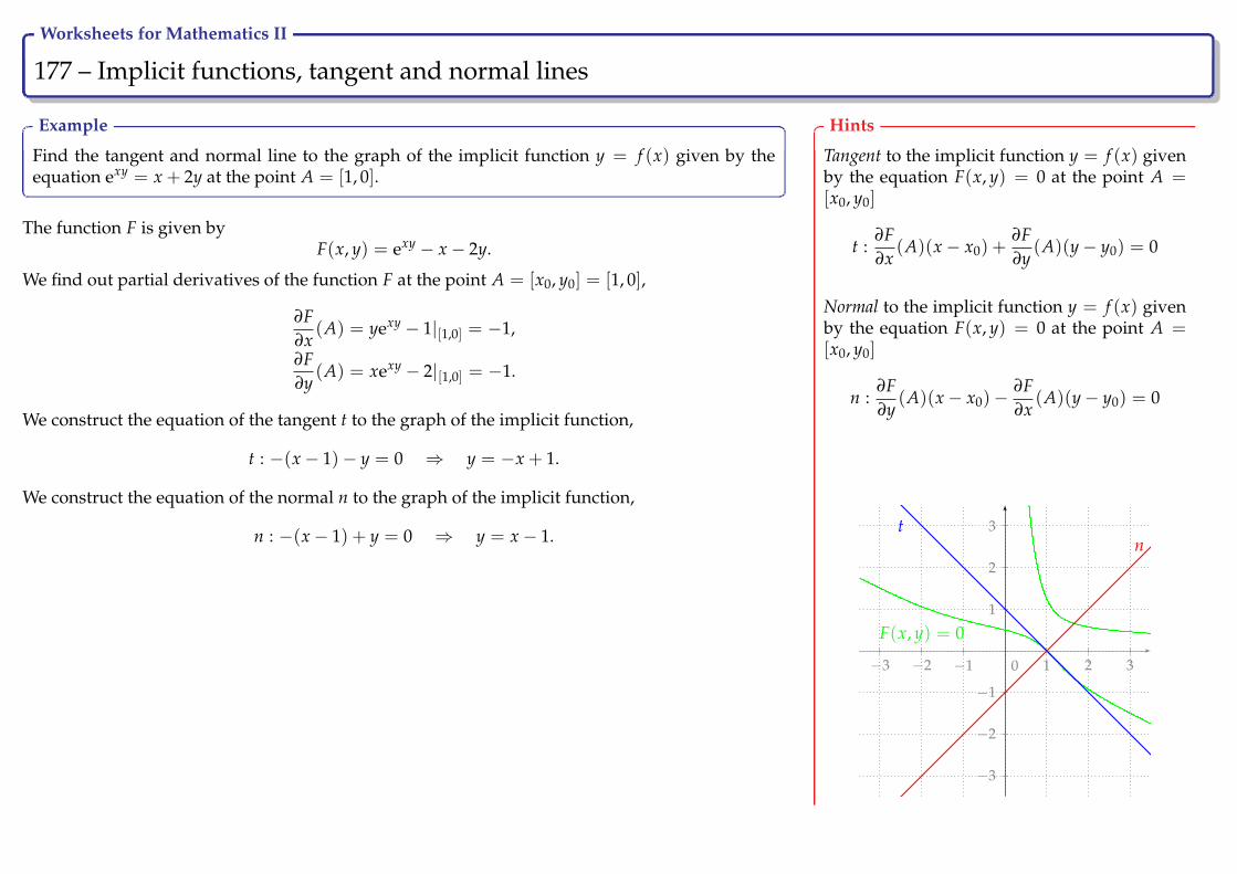
Worksheets for Mathematics II
177 – Implicit functions, tangent and normal lines Ry
Example
Find the tangent and normal line to the graph of the implicit function y = f (x) given by theequation exy = x + 2y at the point A = [1, 0].
The function F is given byF(x, y) = exy − x− 2y.
We find out partial derivatives of the function F at the point A = [x0, y0] = [1, 0],
∂F∂x
(A) = yexy − 1|[1,0] = −1,
∂F∂y
(A) = xexy − 2|[1,0] = −1.
We construct the equation of the tangent t to the graph of the implicit function,
t : −(x− 1)− y = 0 ⇒ y = −x + 1.
We construct the equation of the normal n to the graph of the implicit function,
n : −(x− 1) + y = 0 ⇒ y = x− 1.
Hints
Tangent to the implicit function y = f (x) givenby the equation F(x, y) = 0 at the point A =[x0, y0]
t :∂F∂x
(A)(x− x0) +∂F∂y
(A)(y− y0) = 0
Normal to the implicit function y = f (x) givenby the equation F(x, y) = 0 at the point A =[x0, y0]
n :∂F∂y
(A)(x− x0)−∂F∂x
(A)(y− y0) = 0
−3 −2 −1 1 2 3
−3
−2
−1
1
2
3
0
tn
F(x, y) = 0

Worksheets for Mathematics II
178 – Implicit functions, tangent and normal lines Ry
Exercise
Find the tangent and normal line to the implicit function y = f (x) given byx + yx− y
= 2 at the
point A = [3, 1].
Hints
Tangent to the implicit function y = f (x) givenby the equation F(x, y) = 0 at the point A =[x0, y0]
t :∂F∂x
(A)(x− x0) +∂F∂y
(A)(y− y0) = 0
Normal to the implicit function y = f (x) givenby the equation F(x, y) = 0 at the point A =[x0, y0]
n :∂F∂y
(A)(x− x0)−∂F∂x
(A)(y− y0) = 0

Worksheets for Mathematics II
179 – Implicit functions, tangent and normal lines Ry
Exercise
Find the tangent and normal line to the implicit function y = f (x) given by3xy − 1 = y ln 3 + x ln 3 at the point A = [0, 0].
Hints
Tangent to the implicit function y = f (x) givenby the equation F(x, y) = 0 at the point A =[x0, y0]
t :∂F∂x
(A)(x− x0) +∂F∂y
(A)(y− y0) = 0
Normal to the implicit function y = f (x) givenby the equation F(x, y) = 0 at the point A =[x0, y0]
n :∂F∂y
(A)(x− x0)−∂F∂x
(A)(y− y0) = 0

Worksheets for Mathematics II
180 – Local extrema Ry
Definition
We say that a function z = f (x, y) has local maximum at the point A ∈D f if there exists a neighbourhood O(A) ⊆ D f of the point A such that∀X ∈ O(A) holds f (X) ≤ f (A). If f (X) ≥ f (A) is satisfied ∀X ∈ O(A)then it is local minimum at the point A. In the case of strict inequalitieswe talk about strict local maxima or minima.
Definition
We say that the point A ∈ D f is stationary or critical point of a functionf (x, y) if
∂ f∂x
(A) = 0,∂ f∂y
(A) = 0.
Fermat theorem - necessary condition for existence of an extremum
Theorem (Fermat)
Let a function f has local extremum at the point A and let there exist allpartial derivatives of the first order at the point A. Then the point A isa critical point of the function f .
Remark
• Fermat theorem does not exclude the possibility that the functionf has an extremum at a point which is not the critical point of thefunction f because some of its partial derivatives does not exist.
• The condition for critical points is equivalent with the conditiond f (A) = 0. Nevertheless, if d f (A) 6= 0, then a local extremumdoes not exist at the point A.
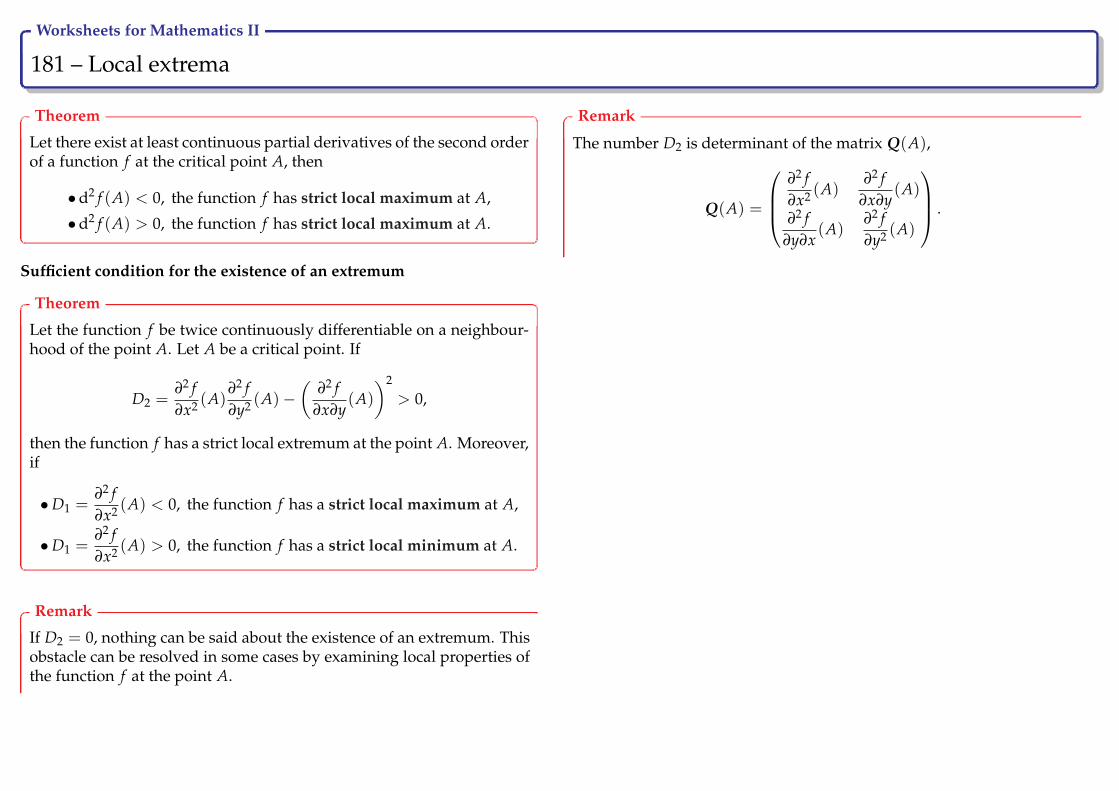
Worksheets for Mathematics II
181 – Local extrema Ry
Theorem
Let there exist at least continuous partial derivatives of the second orderof a function f at the critical point A, then
•d2 f (A) < 0, the function f has strict local maximum at A,
•d2 f (A) > 0, the function f has strict local maximum at A.
Sufficient condition for the existence of an extremum
Theorem
Let the function f be twice continuously differentiable on a neighbour-hood of the point A. Let A be a critical point. If
D2 =∂2 f∂x2 (A)
∂2 f∂y2 (A)−
(∂2 f
∂x∂y(A)
)2
> 0,
then the function f has a strict local extremum at the point A. Moreover,if
•D1 =∂2 f∂x2 (A) < 0, the function f has a strict local maximum at A,
•D1 =∂2 f∂x2 (A) > 0, the function f has a strict local minimum at A.
Remark
If D2 = 0, nothing can be said about the existence of an extremum. Thisobstacle can be resolved in some cases by examining local properties ofthe function f at the point A.
Remark
The number D2 is determinant of the matrix Q(A),
Q(A) =
∂2 f∂x2 (A)
∂2 f∂x∂y
(A)
∂2 f∂y∂x
(A)∂2 f∂y2 (A)
.

Worksheets for Mathematics II
182 – Local extrema 1/2 Ry
Example
Find local extrema of the function z = e−x2−y2(2y2 + x2).
The domain of the function z is the whole set R2. We find partial derivatives of the first order andcreate the system of equations for critical points,
∂ f∂x
= e−x2−y2(−2x)(2y2 + x2) + e−x2−y2
2x = −2xe−x2−y2(2y2 + x2 − 1) = 0,
∂ f∂y
= e−x2−y2(−2y)(2y2 + x2) + e−x2−y2
4y = −2ye−x2−y2(2y2 + x2 − 2) = 0.
The exponential function e−x2−y2is positive, thus
x(2y2 + x2 − 1) = 0,
y(2y2 + x2 − 2) = 0.
Suppose that x = 0. From the second equation y(2y2 − 2) = 0 we get the solutions y = 0 andy = ±1. We got three critical points, A1 = [0, 0], A2 = [0, 1] a A3 = [0,−1].
In the second equation we suppose that y = 0. From the first equation x(x2 − 1) = 0 weget the solutions x = 0 and x = ±1. The point [0, 0] is already found, we have to add two newcritical points A4 = [1, 0] and A5 = [−1, 0].
If x 6= 0 and y 6= 0, we need to solve the following system of equations,
2y2 + x2 − 1 = 0,
2y2 + x2 − 2 = 0.
If we subtract both equations we get 1 = 0, i.e. the solution of the system does not exist.We found five different critical points:
A1 = [0, 0], A2 = [0, 1], A3 = [0,−1], A4 = [1, 0], A5 = [−1, 0].
Hints
• find domain of the function z = f (x, y)
• calculate partial derivatives∂ f∂x
,∂ f∂y
• find critical points A as a solution of thesystem of equations
∂ f∂x
= 0,∂ f∂y
= 0
• create the matrix Q(A) of second orderpartial derivatives at A
Q(A) =
∂2 f∂x2 (A)
∂2 f∂x∂y
(A)
∂2 f∂y∂x
(A)∂2 f∂y2 (A)
• denote
D2 =∂2 f∂x2 (A)
∂2 f∂y2 (A)−
(∂2 f
∂x∂y(A)
)2
D1 =∂2 f∂x2 (A)
• classification
A is not an extremum if D2 < 0A is strict local extremum if D2 > 0A is strict local minimum if moreover D1 > 0A is strict local maximum if moreover D1 < 0

Worksheets for Mathematics II
183 – Local extrema 2/2 Ry
We continue the search for local extrema from the preceding worksheet. We found a total of fivecritical points. We create a matrix of the second order derivatives and we evaluate it at particularcritical points Ai, i = 1, 2, 3, 4, 5,
Q =
(((−2 + 4x2)(2y2 + x2 − 1)− 4x2)e−x2−y2
4xye−x2−y2(2y2 + x2 − 3)
4xye−x2−y2(2y2 + x2 − 3) ((−2 + 4y2)(2y2 + x2 − 2)− 8y2)e−x2−y2
),
Q(A1) =
(2 00 4
), Q(A2) =
(−2
e 00 −8
e
), Q(A3) =
(−2
e 00 −8
e
), Q(A4) =
(−4
e 00 2
e
), Q(A5) =
(−4
e 00 2
e
).
The following table summarizes the classification of extrema at critical points:
Critical point Ai D1 D2 extremum with the value z = f (Ai)
A1 = [0, 0] 2 > 0 8 > 0 strict local minimum z = 0
A2 = [0, 1] −2e < 0 16
e2 > 0 strict local maximum z = 2e
A3 = [0,−1] −2e < 0 16
e2 > 0 strict local maximum z = 2e
A4 = [1, 0] −4e < 0 − 8
e2 < 0 extremum does not exist
A5 = [−1, 0] −4e < 0 − 8
e2 < 0 extremum does not exist
0
0.1
0.2
0.3
0.4
0.5
0.6
0.7
0.8
0
0.1
0.2
0.3
0.4
0.5
0.6
0.7
0.8
A2 =[0, 1, 2
e] A3 =
[0,−1, 2
e]
A1 = [0, 0, 0]
Hints
• find domain of the function z = f (x, y)
• calculate partial derivatives∂ f∂x
,∂ f∂y
• find critical points A as a solution of thesystem of equations
∂ f∂x
= 0,∂ f∂y
= 0
• create the matrix Q(A) of second orderpartial derivatives at A
Q(A) =
∂2 f∂x2 (A)
∂2 f∂x∂y
(A)
∂2 f∂y∂x
(A)∂2 f∂y2 (A)
• denote
D2 =∂2 f∂x2 (A)
∂2 f∂y2 (A)−
(∂2 f
∂x∂y(A)
)2
D1 =∂2 f∂x2 (A)
• classification
A is not an extremum if D2 < 0A is strict local extremum if D2 > 0A is strict local minimum if moreover D1 > 0A is strict local maximum if moreover D1 < 0

Worksheets for Mathematics II
184 – Local extrema Ry
Exercise
Find local extrema of the function z = x2 + 6x + 3y2 − 12y + 11.
Hints
• find domain of the function z = f (x, y)
• calculate partial derivatives∂ f∂x
,∂ f∂y
• find critical points A as a solution of thesystem of equations
∂ f∂x
= 0,∂ f∂y
= 0
• create the matrix Q(A) of second orderpartial derivatives at A
Q(A) =
∂2 f∂x2 (A)
∂2 f∂x∂y
(A)
∂2 f∂y∂x
(A)∂2 f∂y2 (A)
• denote
D2 =∂2 f∂x2 (A)
∂2 f∂y2 (A)−
(∂2 f
∂x∂y(A)
)2
D1 =∂2 f∂x2 (A)
• classification
A is not an extremum if D2 < 0A is strict local extremum if D2 > 0A is strict local minimum if moreover D1 > 0A is strict local maximum if moreover D1 < 0

Worksheets for Mathematics II
185 – Local extrema Ry
Exercise
Find local extrema of the function z = 3xy− x + 2y.
Hints
• find domain of the function z = f (x, y)
• calculate partial derivatives∂ f∂x
,∂ f∂y
• find critical points A as a solution of thesystem of equations
∂ f∂x
= 0,∂ f∂y
= 0
• create the matrix Q(A) of second orderpartial derivatives at A
Q(A) =
∂2 f∂x2 (A)
∂2 f∂x∂y
(A)
∂2 f∂y∂x
(A)∂2 f∂y2 (A)
• denote
D2 =∂2 f∂x2 (A)
∂2 f∂y2 (A)−
(∂2 f
∂x∂y(A)
)2
D1 =∂2 f∂x2 (A)
• classification
A is not an extremum if D2 < 0A is strict local extremum if D2 > 0A is strict local minimum if moreover D1 > 0A is strict local maximum if moreover D1 < 0

Worksheets for Mathematics II
186 – Local extrema Ry
Exercise
Find local extrema of the function z = x2 − xy + 3x + y + 3.
Hints
• find domain of the function z = f (x, y)
• calculate partial derivatives∂ f∂x
,∂ f∂y
• find critical points A as a solution of thesystem of equations
∂ f∂x
= 0,∂ f∂y
= 0
• create the matrix Q(A) of second orderpartial derivatives at A
Q(A) =
∂2 f∂x2 (A)
∂2 f∂x∂y
(A)
∂2 f∂y∂x
(A)∂2 f∂y2 (A)
• denote
D2 =∂2 f∂x2 (A)
∂2 f∂y2 (A)−
(∂2 f
∂x∂y(A)
)2
D1 =∂2 f∂x2 (A)
• classification
A is not an extremum if D2 < 0A is strict local extremum if D2 > 0A is strict local minimum if moreover D1 > 0A is strict local maximum if moreover D1 < 0
Worksheets for Mathematics II
187 – Local extrema Ry
Exercise
Find local extrema of the function z = (x2 + 4x)y + y2.
Hints
• find domain of the function z = f (x, y)
• calculate partial derivatives∂ f∂x
,∂ f∂y
• find critical points A as a solution of thesystem of equations
∂ f∂x
= 0,∂ f∂y
= 0
• create the matrix Q(A) of second orderpartial derivatives at A
Q(A) =
∂2 f∂x2 (A)
∂2 f∂x∂y
(A)
∂2 f∂y∂x
(A)∂2 f∂y2 (A)
• denote
D2 =∂2 f∂x2 (A)
∂2 f∂y2 (A)−
(∂2 f
∂x∂y(A)
)2
D1 =∂2 f∂x2 (A)
• classification
A is not an extremum if D2 < 0A is strict local extremum if D2 > 0A is strict local minimum if moreover D1 > 0A is strict local maximum if moreover D1 < 0
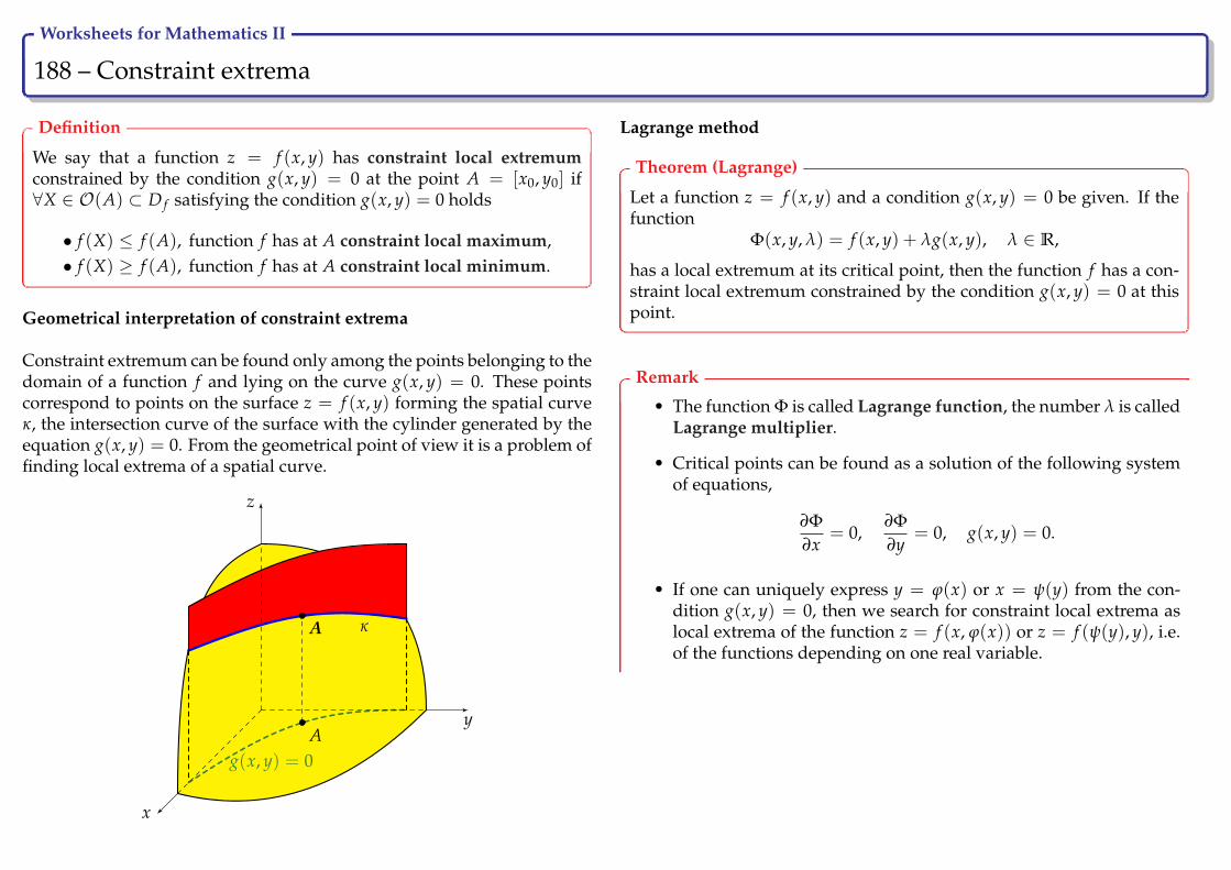
Worksheets for Mathematics II
188 – Constraint extrema Ry
Definition
We say that a function z = f (x, y) has constraint local extremumconstrained by the condition g(x, y) = 0 at the point A = [x0, y0] if∀X ∈ O(A) ⊂ D f satisfying the condition g(x, y) = 0 holds
• f (X) ≤ f (A), function f has at A constraint local maximum,• f (X) ≥ f (A), function f has at A constraint local minimum.
Geometrical interpretation of constraint extrema
Constraint extremum can be found only among the points belonging to thedomain of a function f and lying on the curve g(x, y) = 0. These pointscorrespond to points on the surface z = f (x, y) forming the spatial curveκ, the intersection curve of the surface with the cylinder generated by theequation g(x, y) = 0. From the geometrical point of view it is a problem offinding local extrema of a spatial curve.
κ
g(x, y) = 0
y
z
x
A
A
Lagrange method
Theorem (Lagrange)
Let a function z = f (x, y) and a condition g(x, y) = 0 be given. If thefunction
Φ(x, y, λ) = f (x, y) + λg(x, y), λ ∈ R,
has a local extremum at its critical point, then the function f has a con-straint local extremum constrained by the condition g(x, y) = 0 at thispoint.
Remark
• The function Φ is called Lagrange function, the number λ is calledLagrange multiplier.
• Critical points can be found as a solution of the following systemof equations,
∂Φ∂x
= 0,∂Φ∂y
= 0, g(x, y) = 0.
• If one can uniquely express y = ϕ(x) or x = ψ(y) from the con-dition g(x, y) = 0, then we search for constraint local extrema aslocal extrema of the function z = f (x, ϕ(x)) or z = f (ψ(y), y), i.e.of the functions depending on one real variable.

Worksheets for Mathematics II
189 – Constraint extrema Ry
Example
Find constraint local extrema of z = f (x, y) =√
4x + y2 + 5 with respect to the condition 2x− 3− y = 0.
We find domain of the function z,
4x + y2 + 5 ≥ 0 ⇒ x ≥ −14
y2 − 54
, see the figure in Hints.
From the equation of the constraint 2x− 3− y = 0 one can uniquely express both y and x. Let express y,
y = 2x− 3.
We substitute the constraint in the function z,
z =√
4x + (2x− 3)2 + 5 =√
4x + 4x2 − 12x + 9 + 5 =√
4x2 − 8x + 14,
we get the function z = z(x, ϕ(x)) depending only on one variable and we see that Dz = R. We calculate thefirst order derivative, we set this derivate equal to zero and finally obtain the equation for critical points of thisfunction,
z′ =dzdx
=8x− 8
2√
4x2 − 8x + 14=
4x− 4√4x2 − 8x + 14
= 0 ⇒ 4x− 4 = 0⇒ x = 1.
Domain of the first order derivative is the set Dz′ = R. On the interval (−∞, 1) the derivative is negative,z′ < 0, the function z is a decreasing function on this interval. On the interval (1, ∞) the first derivative ispositive, z′ > 0, i.e. the function z is an increasing function on this interval. At the critical point x = 1 thederivative changes its sign from − to +, it means that at the point x = 1 the function z has a local minimum.
We substitute the point x = 1 into the equation of the constraint, we get y = −1. It is easy to checkthat the point A belongs to domain of the function z =
√4x + y2 + 5, see figure in Hints.
The function z =√
4x + y2 + 5 has constraint local minimum z = f (1,−1) =√
10 at the point A = [1,−1].
Quite analogously we can proceed if we choose the unique expression of x from the equation of theconstraint at the beginning.
Hints
If one can uniquely express fromthe constraint condition x or y, weneed to follow the steps:
• we express either y = ϕ(x) orx = ψ(y)
• constraint local extrema aresearched as local extrema ofthe function depending onone real variable, either z =f (x, ϕ(x)) or z = f (ψ(y), y)
0
y2 ≥ −4x− 5
A
−4 −3 −2 −1 1
−3
−2
−1
1
2
3

Worksheets for Mathematics II
190 – Constraint extrema Ry
Example
Find constraint local extrema of z = f (x, y) = −8x + 6y− 5 with respect to the condition x2 + y2 = 100.
We construct Lagrange function for f (x) = −8x + 6y− 5 and g(x, y) = x2 + y2 − 100,
Φ(x, y, λ) = −8x + 6y− 5 + λ(x2 + y2 − 100).
We calculate first order partial derivatives of Φ and create equations for critical points of Φ,
∂Φ∂x
= −8 + 2λx = 0,∂Φ∂y
= 6 + 2λy = 0,
we solve the following system
−8 + 2λx = 0 ⇒ x =4λ
6 + 2λy = 0 ⇒ y = − 3λ
we substitute into the constraint equation instead of x and y,
x2 + y2 = 100 ⇒(
4λ
)2
+
(− 3
λ
)2
= 100 ⇒ 16λ2 +
9λ2 = 100⇒ 100λ2 = 25⇒ λ2 =
14⇒ λ1,2 = ±1
2.
We calculate critical points A = [x, y] substituting λ,
λ1 =12⇒ A1 = [8,−6], λ2 = −1
2⇒ A2 = [−8, 6].
We construct classification matrix and evaluate this matrix at critical points,
Q =
∂2Φ∂x2
∂2Φ∂x∂y
∂2Φ∂y∂x
∂2Φ∂y2
=
(2λ 00 2λ
), Q(A1) =
(1 00 1
), Q(A2) =
(−1 00 −1
).
At A1 = [8,−6] is D1 > 0, D2 > 0. The function z = f (x, y) has constraint local minimum z = −105 atA1 = [8,−6]. At the point A2 = [−8, 6] is D1 < 0, D2 > 0. The function z = f (x, y) has constraint localmaximum z = 95 at A2 = [−8, 6].
Hints
In the case when one can uniquelyexpress from the constraint equa-tion g(x, y) = 0 neither x nor y weneed to follow the steps:
• we construct Lagrange func-tion
Φ(x, y, λ) = f (x, y) + λg(x, y)
• we search for local extrema ofthe function Φ
• if the function Φ has in its crit-ical point a local extremum,then the function z = f (x, y)has constraint local extremumconstrained by the conditiong(x, y) = 0 at this point.
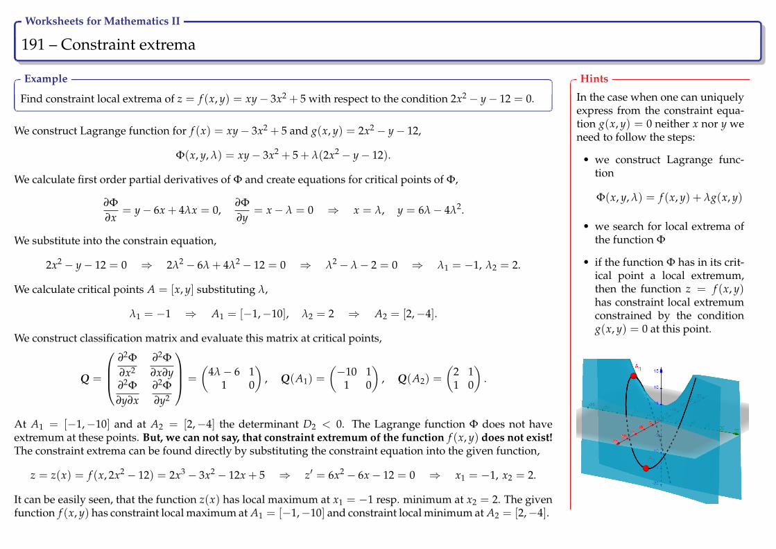
Worksheets for Mathematics II
191 – Constraint extrema Ry
Example
Find constraint local extrema of z = f (x, y) = xy− 3x2 + 5 with respect to the condition 2x2 − y− 12 = 0.
We construct Lagrange function for f (x) = xy− 3x2 + 5 and g(x, y) = 2x2 − y− 12,
Φ(x, y, λ) = xy− 3x2 + 5 + λ(2x2 − y− 12).
We calculate first order partial derivatives of Φ and create equations for critical points of Φ,
∂Φ∂x
= y− 6x + 4λx = 0,∂Φ∂y
= x− λ = 0 ⇒ x = λ, y = 6λ− 4λ2.
We substitute into the constrain equation,
2x2 − y− 12 = 0 ⇒ 2λ2 − 6λ + 4λ2 − 12 = 0 ⇒ λ2 − λ− 2 = 0 ⇒ λ1 = −1, λ2 = 2.
We calculate critical points A = [x, y] substituting λ,
λ1 = −1 ⇒ A1 = [−1,−10], λ2 = 2 ⇒ A2 = [2,−4].
We construct classification matrix and evaluate this matrix at critical points,
Q =
∂2Φ∂x2
∂2Φ∂x∂y
∂2Φ∂y∂x
∂2Φ∂y2
=
(4λ− 6 1
1 0
), Q(A1) =
(−10 1
1 0
), Q(A2) =
(2 11 0
).
At A1 = [−1,−10] and at A2 = [2,−4] the determinant D2 < 0. The Lagrange function Φ does not haveextremum at these points. But, we can not say, that constraint extremum of the function f (x, y) does not exist!The constraint extrema can be found directly by substituting the constraint equation into the given function,
z = z(x) = f (x, 2x2 − 12) = 2x3 − 3x2 − 12x + 5 ⇒ z′ = 6x2 − 6x− 12 = 0 ⇒ x1 = −1, x2 = 2.
It can be easily seen, that the function z(x) has local maximum at x1 = −1 resp. minimum at x2 = 2. The givenfunction f (x, y) has constraint local maximum at A1 = [−1,−10] and constraint local minimum at A2 = [2,−4].
Hints
In the case when one can uniquelyexpress from the constraint equa-tion g(x, y) = 0 neither x nor y weneed to follow the steps:
• we construct Lagrange func-tion
Φ(x, y, λ) = f (x, y) + λg(x, y)
• we search for local extrema ofthe function Φ
• if the function Φ has in its crit-ical point a local extremum,then the function z = f (x, y)has constraint local extremumconstrained by the conditiong(x, y) = 0 at this point.
Worksheets for Mathematics II
192 – Constraint extrema Ry
Exercise
Find constraint extrema of the function z = f (x, y) with respect to the condition g(x, y) = 0:
a) z = 4x + 2y + 1, y = x2 + x +14
b) z = 12x + y− 3, y = −x3 + 3
Hints
If one can uniquely express fromthe constraint condition x or y, weneed to follow the steps:
• we express either y = ϕ(x) orx = ψ(y)
• constraint local extrema aresearched as local extrema ofthe function depending onone real variable, either z =f (x, ϕ(x)) or z = f (ψ(y), y)

Worksheets for Mathematics II
193 – Constraint extrema Ry
Exercise
Find constraint extrema of the function z = 4x + 3y− 4 with respect to the condition (x− 1)2 + (y− 2)2 = 1.
Hints
In the case when one can uniquelyexpress from the constraint equa-tion g(x, y) = 0 neither x nor y weneed to follow the steps:
• we construct Lagrange func-tion
Φ(x, y, λ) = f (x, y) + λg(x, y)
• we search for local extrema ofthe function Φ
• if the function Φ has in its crit-ical point a local extremum,then the function z = f (x, y)has constraint local extremumconstrained by the conditiong(x, y) = 0 at this point.
Worksheets for Mathematics II
194 – Global extrema Ry
Definition
We say that a function z = f (x, y) has global extremum at the pointA = [x0, y0] on closed domain D f if ∀X ∈ D f holds
• f (X) ≤ f (A), f has global maximum at the point A,• f (X) ≥ f (A), f has global minimum at the point A.
Remark
• In the case of strict inequalities we talk about strict global ex-tremum.
• Domain D f is called closed, if it contains all its boundary points.Boundary point of the set D f is a point, such that its every neigh-bourhood contains points X satisfying X ∈ D f and at the sametime it contains points Y satisfying Y 6∈ D f .
Algorithm
• we find domain D f of the function z = f (x, y),
• we find local extrema of the function z on the domain D f from whichwe exclude boundary g(x, y) = 0,
• we find constraint extrema of the function with respect to the condi-tion g(x, y) = 0,
• we compare all function values at extrema points, the point with thelargest function value is global maximum, the point with the smallestfunction value is global minimum.
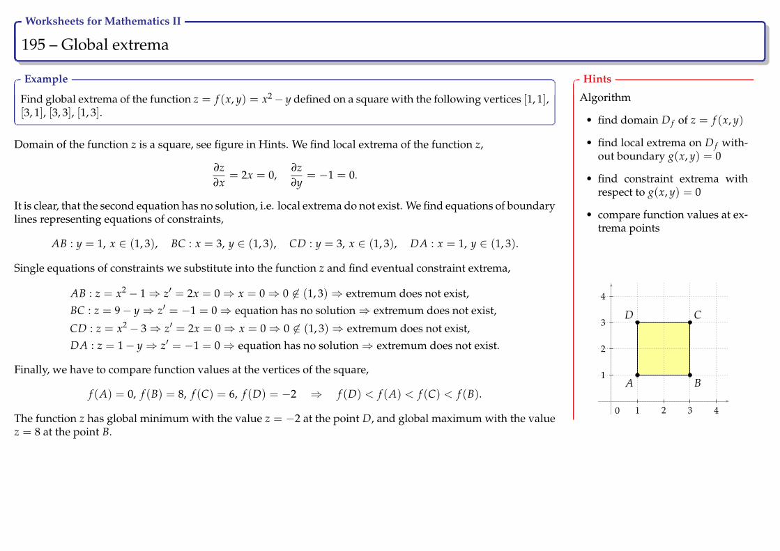
Worksheets for Mathematics II
195 – Global extrema Ry
Example
Find global extrema of the function z = f (x, y) = x2− y defined on a square with the following vertices [1, 1],[3, 1], [3, 3], [1, 3].
Domain of the function z is a square, see figure in Hints. We find local extrema of the function z,
∂z∂x
= 2x = 0,∂z∂y
= −1 = 0.
It is clear, that the second equation has no solution, i.e. local extrema do not exist. We find equations of boundarylines representing equations of constraints,
AB : y = 1, x ∈ (1, 3), BC : x = 3, y ∈ (1, 3), CD : y = 3, x ∈ (1, 3), DA : x = 1, y ∈ (1, 3).
Single equations of constraints we substitute into the function z and find eventual constraint extrema,
AB : z = x2 − 1⇒ z′ = 2x = 0⇒ x = 0⇒ 0 6∈ (1, 3)⇒ extremum does not exist,
BC : z = 9− y⇒ z′ = −1 = 0⇒ equation has no solution⇒ extremum does not exist,
CD : z = x2 − 3⇒ z′ = 2x = 0⇒ x = 0⇒ 0 6∈ (1, 3)⇒ extremum does not exist,
DA : z = 1− y⇒ z′ = −1 = 0⇒ equation has no solution⇒ extremum does not exist.
Finally, we have to compare function values at the vertices of the square,
f (A) = 0, f (B) = 8, f (C) = 6, f (D) = −2 ⇒ f (D) < f (A) < f (C) < f (B).
The function z has global minimum with the value z = −2 at the point D, and global maximum with the valuez = 8 at the point B.
Hints
Algorithm
• find domain D f of z = f (x, y)
• find local extrema on D f with-out boundary g(x, y) = 0
• find constraint extrema withrespect to g(x, y) = 0
• compare function values at ex-trema points
0
A B
CD
−1 1 2 3 4
−1
1
2
3
4

Worksheets for Mathematics II
196 – Global extrema Ry
Exercise
Find global extrema of the function z = −x2 − y2 + 2y on the circle x2 + y2 ≤ 16.
Hints
Algorithm
• find domain D f of z = f (x, y)
• find local extrema on D f with-out boundary g(x, y) = 0
• find constraint extrema withrespect to g(x, y) = 0
• compare function values at ex-trema points

Worksheets for Mathematics II
197 – Global extrema Ry
Exercise
Find global extrema of the function z = x2 + y2 on the triangle with the vertices at [0, 0], [2, 0] and [0, 1].
Hints
Algorithm
• find domain D f of z = f (x, y)
• find local extrema on D f with-out boundary g(x, y) = 0
• find constraint extrema withrespect to g(x, y) = 0
• compare function values at ex-trema points
Worksheets for Mathematics II
Ordinary differential equations
Worksheets for Mathematics II
199 – Differential equations of the n-th order Ry
Differential equations are equations in which one can find independent,dependent variables and derivatives of dependent variable with respectto the independent one. Differential equations contain derivatives. Dif-ferential equations represent a relation between unknown function and itsderivatives.
Definition
Any equation of the form
F(x, y, y′, , . . . , y(n−1), y(n)) = 0
is called n-th order ordinary differential equation for unknown func-tion y = y(x).
The order of the differential equation is the order of the highest derivativeof unknown function y(x) in the ordinary differential equation.
Solution (integral) of differential equation on the interval I is everyfunction y(x), which has continuous derivatives up to order n and solvesthe given differential equation.
We distinguish the following types of solutions:
• general solution of an n-th order differential equation represents theset of functions of the form
Φ(x, y, C1, C2, . . . , Cn) = 0, resp. y = ϕ(x, C1, C2, . . . , Cn),
i.e. the set of functions containing n real constants C1, C2, . . . , Cn,
• particular solution yp is one concrete solution, which can be ob-tained from a general solution by the choice or calculation of inte-gration constants C1, C2, . . . , Cn,
• singular solution is a solution, which cannot be obtained from a gen-eral solution by any choice of integration constants C1, C2, . . . , Cn.
Remark
• For simplicity, instead of ordinary differential equations we usewords differential equations. There exist also partial differentialequations, but those equations will not be discussed. Thus, thereis no need to distinguish between ordinary and particular differ-ential equations.
• It is common to use instead of ordinary differential equations theabbreviation ODE.
Worksheets for Mathematics II
200 – Differential equation of the 3-rd order - direct integration Ry
Example
Find at least one particular solution of ODE y′′′ = 6x− 6.
Given differential equation can be integrated directly, i.e. one can integrate simultaneously both sides of the
equation. Recall a relation between derivatives and differentials, y′ =d
dx(y).
y′′ =∫
y′′′ dx =∫(6x− 6)dx ⇒ y′′ = 3x2 − 6x + C1.
Using the same way, we can subsequently reduce the order of the given ODE. Thus,
y′ =∫
y′′ dx =∫(3x2 − 6x + C1)dx ⇒ y′ = x3 − 3x2 + C1x + C2,
y =∫
y′ dx =∫(x3 − 3x2 + C1x + C2)dx ⇒ y =
x4
4− x3 + C1
x2
2+ C2x + C3.
We see three integration constants C1, C2, C3 in the general solution.
By the particular solution we mean a concrete curve. This curve can be obtained by arbitrary choice of theintegration constants C1, C2 and C3, e.g. for C1 = 2, C2 = 3 a C3 = 5 we get the particular solution of the form
yp =x4
4− x3 + x2 + 3x + 5.
Note that in concrete practical situations the choice of integration constants is not arbitrary and is strictly con-nected with the solved problem.
Hints
Direct integration
ODE of the type y(n) = f (x)
n-th order derivative
y(n) =d
dx
(y(n−1)
)
General solution
y =∫· · ·
∫︸ ︷︷ ︸
n-times
f (x)dx . . . dx︸ ︷︷ ︸n-times
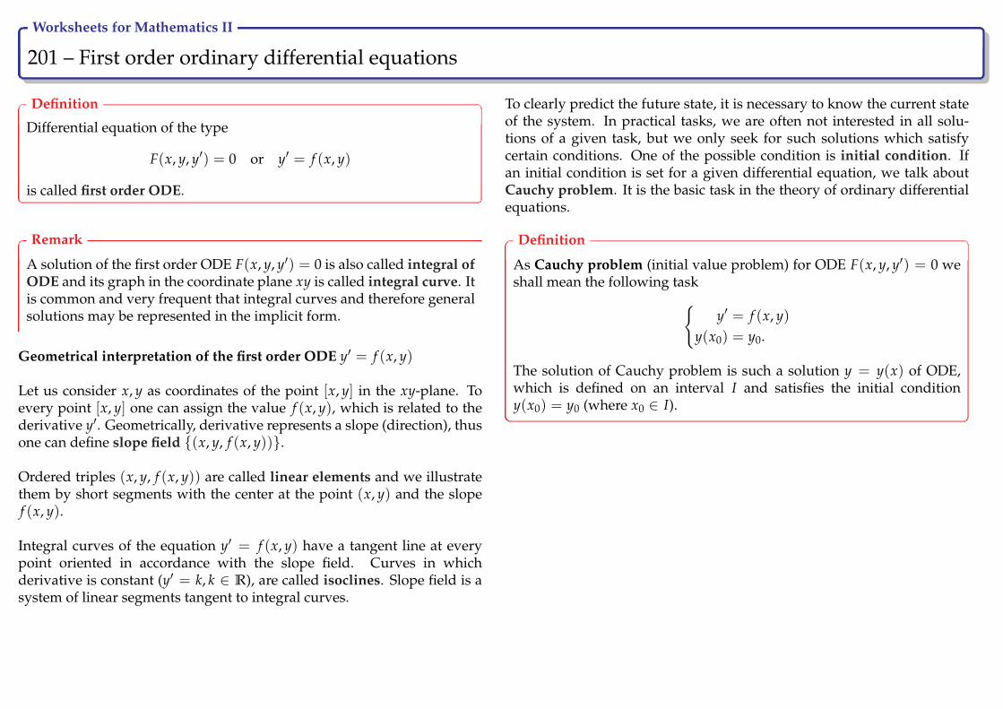
Worksheets for Mathematics II
201 – First order ordinary differential equations Ry
Definition
Differential equation of the type
F(x, y, y′) = 0 or y′ = f (x, y)
is called first order ODE.
Remark
A solution of the first order ODE F(x, y, y′) = 0 is also called integral ofODE and its graph in the coordinate plane xy is called integral curve. Itis common and very frequent that integral curves and therefore generalsolutions may be represented in the implicit form.
Geometrical interpretation of the first order ODE y′ = f (x, y)
Let us consider x, y as coordinates of the point [x, y] in the xy-plane. Toevery point [x, y] one can assign the value f (x, y), which is related to thederivative y′. Geometrically, derivative represents a slope (direction), thusone can define slope field (x, y, f (x, y)).
Ordered triples (x, y, f (x, y)) are called linear elements and we illustratethem by short segments with the center at the point (x, y) and the slopef (x, y).
Integral curves of the equation y′ = f (x, y) have a tangent line at everypoint oriented in accordance with the slope field. Curves in whichderivative is constant (y′ = k, k ∈ R), are called isoclines. Slope field is asystem of linear segments tangent to integral curves.
To clearly predict the future state, it is necessary to know the current stateof the system. In practical tasks, we are often not interested in all solu-tions of a given task, but we only seek for such solutions which satisfycertain conditions. One of the possible condition is initial condition. Ifan initial condition is set for a given differential equation, we talk aboutCauchy problem. It is the basic task in the theory of ordinary differentialequations.
Definition
As Cauchy problem (initial value problem) for ODE F(x, y, y′) = 0 weshall mean the following task
y′ = f (x, y)y(x0) = y0.
The solution of Cauchy problem is such a solution y = y(x) of ODE,which is defined on an interval I and satisfies the initial conditiony(x0) = y0 (where x0 ∈ I).

Worksheets for Mathematics II
202 – Slope field Ry
Example
Use isoclines to draw a slope filed of the first order ODE y′ = x−√y.
The function f (x, y) = x−√y is defined ∀x ∈ R and y ≥ 0.
We find isoclines in such a way that we set the function equal to a constant and evaluate y.
x−√y = k ⇒ √y = x− k ⇒ y = (x− k)2; k ∈ R, x ≥ k.
It is a right part of a parabola curve with vertex at the point [k, 0].
x
y
Isoclines of the equation y′ = x−√y.
x
y
Slope field of the equation y′ = x−√y.
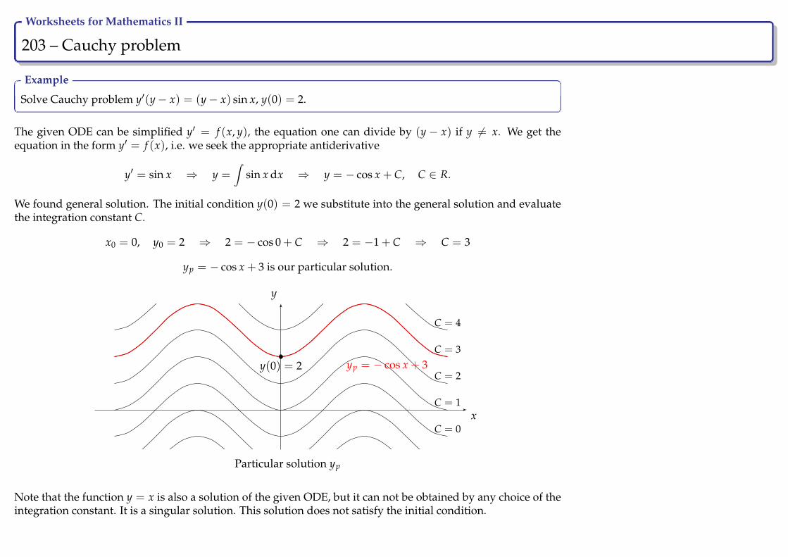
Worksheets for Mathematics II
203 – Cauchy problem Ry
Example
Solve Cauchy problem y′(y− x) = (y− x) sin x, y(0) = 2.
The given ODE can be simplified y′ = f (x, y), the equation one can divide by (y − x) if y 6= x. We get theequation in the form y′ = f (x), i.e. we seek the appropriate antiderivative
y′ = sin x ⇒ y =∫
sin x dx ⇒ y = − cos x + C, C ∈ R.
We found general solution. The initial condition y(0) = 2 we substitute into the general solution and evaluatethe integration constant C.
x0 = 0, y0 = 2 ⇒ 2 = − cos 0 + C ⇒ 2 = −1 + C ⇒ C = 3
yp = − cos x + 3 is our particular solution.
x
y
C = −2
C = −1
C = 0
C = 1
C = 2
C = 3
C = 4
y(0) = 2 yp = − cos x + 3
Particular solution yp
Note that the function y = x is also a solution of the given ODE, but it can not be obtained by any choice of theintegration constant. It is a singular solution. This solution does not satisfy the initial condition.

Worksheets for Mathematics II
204 – Separable differential equations Ry
Definition
By differential equation with separated variables we shall mean everyequation which can be expressed in the form
Q(y)y′ = P(x), i.e. Q(y)dy = P(x)dx,
if we use instead of derivative y′ quotientdydx
.
It can be immediately seen that the variables are separated on both sidesof the equation and one can directly integrate them. This leads to∫
Q(y)dy =∫
P(x)dx + C.
Note that we consider the only one integration constant, usually weadd this integration constant to the right side of the equation, where theindependent variable x is presented.
In practice, we encounter a lot of problems that can be converted toa separated differential equation with the help of simple manipulations.Such equations are called separable. We distinguish three types ofseparable ODE:
• y′ = f (x)g(y),
• y′ = f (ax + by + c),
• y′ = f( y
x), called homogeneous ODE.

Worksheets for Mathematics II
205 – Separable ODE of the type y′ = f (x)g(y) Ry
The equation y′ = f (x)g(y) assuming g(y) 6= 0 and using identity y′ =dydx
can be rewritten as follows:
dyg(y)
= f (x)dx,
which is ODE with separated variables. Its general solution can be writtenas ∫ dy
g(y)=∫
f (x)dx + C.
Remark
The shape of the general solution should be adjusted in some case. Weget a logarithmic function on the left-hand side after the integration.In this case, as a logarithmic function by the relation A = ln eAwe alsoexpress the right-hand side of the solution.
Assume that the general solution is of the form ln m(y) = n(x) + C. Weintroduce a logarithmic function on the right-hand side
ln m(y) = ln en(x)+C ⇒ ln m(y) = ln(
en(x)eC)
.
From the equality of logarithms it follows
m(y) = en(x)eC.
Without loss of generality it is common to label new constant eC like theoriginal constant “eC = C”. Thus the solution takes the form
m(y) = Cen(x).

Worksheets for Mathematics II
206 – Separable ODE of the type y′ = f (x)g(y) Ry
Example
Find the general solution of ODE y′ =x− e−x
y + ey .
We rewrite the ODE to the form y′ = (x − e−x) · 1y + ey where it is easy to see that the equation is of form
y′ = f (x)g(y). We are going to solve it by the method of separation of variables,
y′ =x− e−x
y + ey ⇒ dydx
=x− e−x
y + ey ⇒ (y + ey)dy = (x− e−x)dx.
After the integration of both sides of the equation we get∫(y + ey)dy =
∫(x− e−x)dx + C ⇒ y2
2+ ey =
x2
2+ e−x + C.
The general solution takes the formy2
2− x2
2+ ey − e−x = C.
x
y
C > 0
C < 0C = 0
General solution y
Hints
Separable differential equation
of the type y′ = P(x)Q(y)
derivative
y′ =dydx
general solution∫ dyQ(y)
=∫
P(x)dx + C,
for Q(y) 6= 0

Worksheets for Mathematics II
207 – Separable ODE of the type y′ = f (x)g(y) Ry
Example
Solve the Cauchy problemy′
y= −2 sin x, y (π) = 1.
It is a separable ODE,
y′
y= −2 sin x ⇒ 1
ydydx
= −2 sin x ⇒ 1y
dy = −2 sin x dx.
After the integration we get∫ 1y
dy = −2∫
sin x dx + C ⇒ ln |y| = 2 cos x + C.
We rewrite the general solution
ln |y| = 2 cos x + C ⇒ y = Ce2 cos x.
We find the value for C using the initial condition, i.e. x = π, y = 1,
1 = Ce2 cos π ⇒ C = e2.
Finally, the particular solution takes the form
yp = e2e2 cos x ⇒ yp = e2 cos x+2.
Hints
Separable differential equation
of the type y′ = P(x)Q(y)
derivative
y′ =dydx
general solution∫ dyQ(y)
=∫
P(x)dx + C,
for Q(y) 6= 0

Worksheets for Mathematics II
208 – Separable ODE of the type y′ = f (x)g(y) Ry
Example
How long does it take for the temperature of the heated body to drop from 90 C to 50 C, if the temperatureof environment is equal to 25 C and in the first 10 minutes the body cooled down to 73 C.
Speed of cooling of a body is represented by a decrease of temperature τ in time t and is given by the derivativedτ
dt. Newton’s law of cooling states that speed of cooling is proportional to a difference between the temperature
of the body and the temperature of environment. If we assume that the temperature of environment is constant,the differential equation of cooling takes the form
dτ
dt= −k(τ − τ0), with τ temp. of the body, τ0 temp. of environment and k > 0 is coefficient of proportionality.
The equation can be solved by separation of variables method:
dτ
τ − τ0= −k dt ⇒ ln |τ − τ0| = −kt + c ⇒ τ = τ0 + c1e−kt.
We use the initial condition to find the value for the integration constant c1, at t0 = 0 is τ = 90 and τ0 = 25,
90 = 25 + c1e−k·0 ⇒ c1 = 65.
We see that at the time t = 10 is τ = 73 and τ0 = 25, we use this values to find k and finally the relation betweenτ and t:
73 = 25 + 65e−k·10 ⇒ e−k·10 =4865⇒
(e−k)10
=4865⇒ e−k =
(4865
) 110
⇒ τ = 25 + 65 ·(
4865
) t10
.
We find the time t of cooling the body for τ = 50:
50 = 25 + 65 ·(
4865
) t10
⇒ 513
=
(4865
) t10
⇒(
513
)10
=
(4865
)t⇒ t =
10 ln 513
ln 4865
= 31.5 min.
The body is cooled down to 50 C in 31 minutes and 30 seconds.
Hints
Separable differential equation
of the type y′ = P(x)Q(y)
derivative
y′ =dydx
general solution∫ dyQ(y)
=∫
P(x)dx + C,
for Q(y) 6= 0
t
τ
0 10
73
90
50
?
Cooling curve
Worksheets for Mathematics II
209 – Separable ODE of the type y′ = f (x)g(y) Ry
Exercise
Solve the differential equations:
a) y′ sin x = y cos x b) x2y′ − y2 = 1 c) 2xyy′ = x + 2
Hints
Separable differential equation
of the type y′ = P(x)Q(y)
derivative
y′ =dydx
general solution∫ dyQ(y)
=∫
P(x)dx + C,
for Q(y) 6= 0
Worksheets for Mathematics II
210 – Separable ODE of the type y′ = f (x)g(y) Ry
Exercise
Solve the Cauchy problems:
a) y′ + ey = 0, y(0) = 0 b) y′ sin x = y ln y, y(π2 ) = e c) y− xy′ = 5(1 + x2y′), y(1) = 1
Hints
Separable differential equation
of the type y′ = P(x)Q(y)
derivative
y′ =dydx
general solution∫ dyQ(y)
=∫
P(x)dx + C,
for Q(y) 6= 0

Worksheets for Mathematics II
211 – Separable ODE of the type y′ = f (ax + by + c) Ry
Differential equations of the form y′ = f (ax + by + c), where b 6= 0, can betransformed to a differential equation with separated variables by meansof the substitution u(x) = ax + by + c. Substitution gives the formula forthe derivative y′.
We differentiate the equality u(x) = ax + by + c with respect to x andexpress y′,
u′ = a + by′ ⇒ y′ =u′ − a
b.
After the substitution into the original differential equation we get a dif-ferential equation with separable variables of the form u′ = f (x)g(u),
u′ − ab
= f (u) ⇒ u′ = a + b f (u).
For a + b f (u) 6= 0 we get the equation
1a + b f (u)
u′ = 1.
Its general solution then takes the form∫ dua + b f (u)
= x + C.
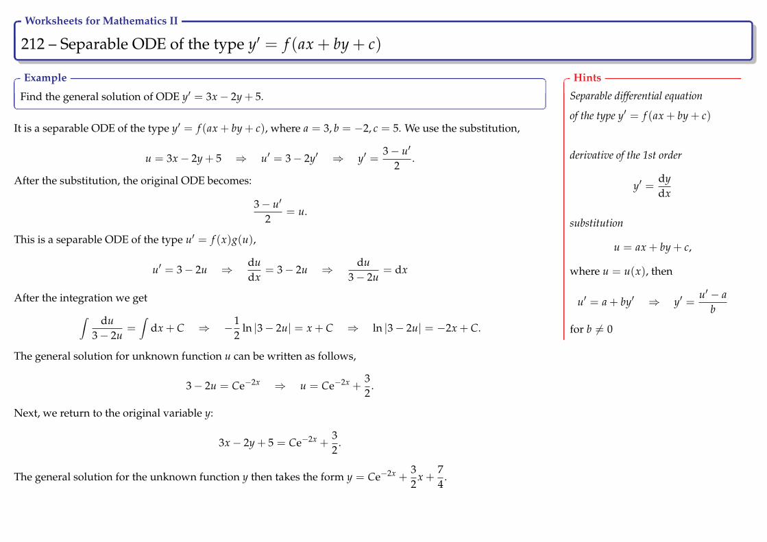
Worksheets for Mathematics II
212 – Separable ODE of the type y′ = f (ax + by + c) Ry
Example
Find the general solution of ODE y′ = 3x− 2y + 5.
It is a separable ODE of the type y′ = f (ax + by + c), where a = 3, b = −2, c = 5. We use the substitution,
u = 3x− 2y + 5 ⇒ u′ = 3− 2y′ ⇒ y′ =3− u′
2.
After the substitution, the original ODE becomes:
3− u′
2= u.
This is a separable ODE of the type u′ = f (x)g(u),
u′ = 3− 2u ⇒ dudx
= 3− 2u ⇒ du3− 2u
= dx
After the integration we get∫ du3− 2u
=∫
dx + C ⇒ −12
ln |3− 2u| = x + C ⇒ ln |3− 2u| = −2x + C.
The general solution for unknown function u can be written as follows,
3− 2u = Ce−2x ⇒ u = Ce−2x +32
.
Next, we return to the original variable y:
3x− 2y + 5 = Ce−2x +32
.
The general solution for the unknown function y then takes the form y = Ce−2x +32
x +74
.
Hints
Separable differential equation
of the type y′ = f (ax + by + c)
derivative of the 1st order
y′ =dydx
substitution
u = ax + by + c,
where u = u(x), then
u′ = a + by′ ⇒ y′ =u′ − a
b
for b 6= 0
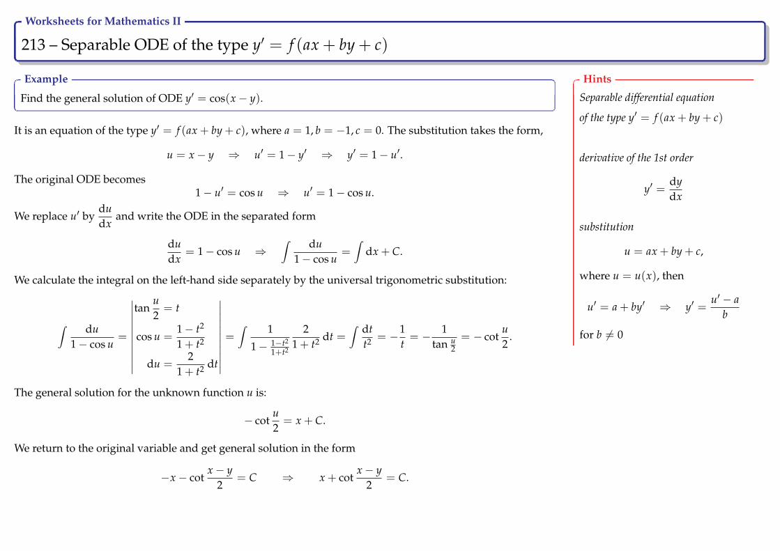
Worksheets for Mathematics II
213 – Separable ODE of the type y′ = f (ax + by + c) Ry
Example
Find the general solution of ODE y′ = cos(x− y).
It is an equation of the type y′ = f (ax + by + c), where a = 1, b = −1, c = 0. The substitution takes the form,
u = x− y ⇒ u′ = 1− y′ ⇒ y′ = 1− u′.
The original ODE becomes1− u′ = cos u ⇒ u′ = 1− cos u.
We replace u′ bydudx
and write the ODE in the separated form
dudx
= 1− cos u ⇒∫ du
1− cos u=∫
dx + C.
We calculate the integral on the left-hand side separately by the universal trigonometric substitution:
∫ du1− cos u
=
∣∣∣∣∣∣∣∣∣∣∣
tanu2= t
cos u =1− t2
1 + t2
du =2
1 + t2 dt
∣∣∣∣∣∣∣∣∣∣∣=∫ 1
1− 1−t2
1+t2
21 + t2 dt =
∫ dtt2 = −1
t= − 1
tan u2= − cot
u2
.
The general solution for the unknown function u is:
− cotu2= x + C.
We return to the original variable and get general solution in the form
−x− cotx− y
2= C ⇒ x + cot
x− y2
= C.
Hints
Separable differential equation
of the type y′ = f (ax + by + c)
derivative of the 1st order
y′ =dydx
substitution
u = ax + by + c,
where u = u(x), then
u′ = a + by′ ⇒ y′ =u′ − a
b
for b 6= 0
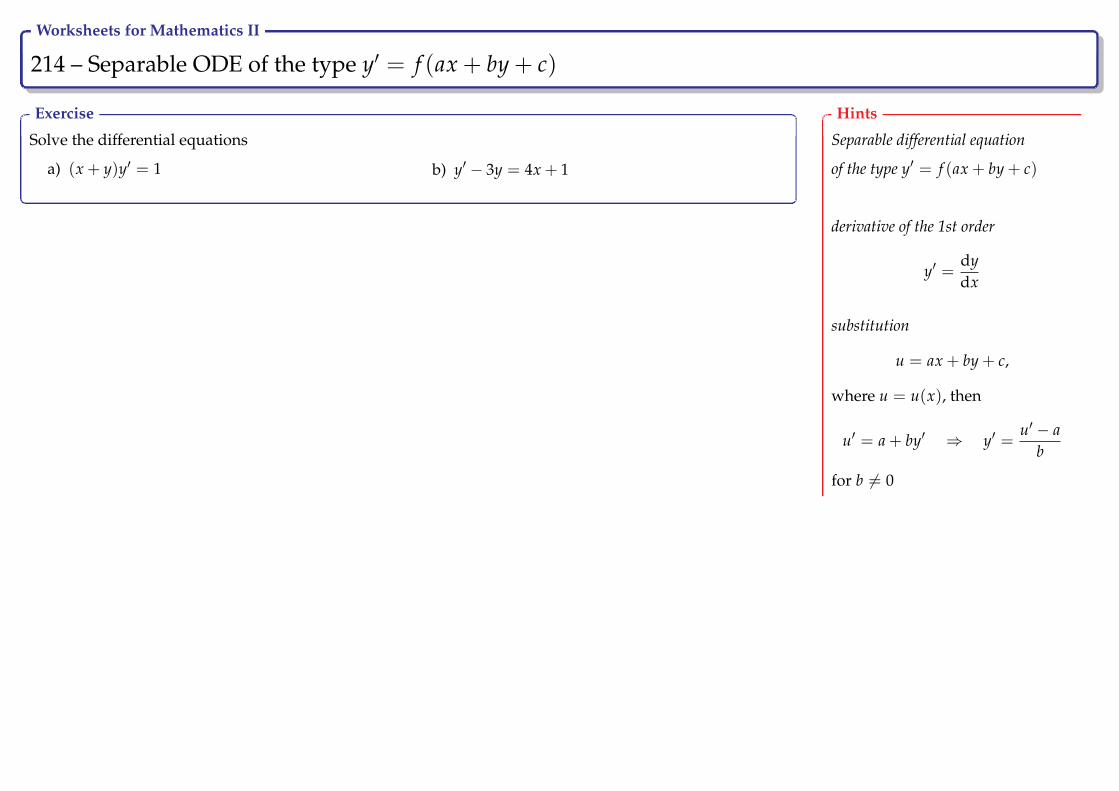
Worksheets for Mathematics II
214 – Separable ODE of the type y′ = f (ax + by + c) Ry
Exercise
Solve the differential equations
a) (x + y)y′ = 1 b) y′ − 3y = 4x + 1
Hints
Separable differential equation
of the type y′ = f (ax + by + c)
derivative of the 1st order
y′ =dydx
substitution
u = ax + by + c,
where u = u(x), then
u′ = a + by′ ⇒ y′ =u′ − a
b
for b 6= 0

Worksheets for Mathematics II
215 – Separable ODE of the type y′ = f (ax + by + c) Ry
Exercise
Solve the differential equations
a) y′ = sin2(x− y) b) y′√
1 + x + y = x + y + 1
Hints
Separable differential equation
of the type y′ = f (ax + by + c)
derivative of the 1st order
y′ =dydx
substitution
u = ax + by + c,
where u = u(x), then
u′ = a + by′ ⇒ y′ =u′ − a
b
for b 6= 0

Worksheets for Mathematics II
216 – Separable ODE of the type y′ = f (yx) Ry
Definition
The differential equation F(x, y, y′) = 0 is called homogeneous, if it canbe written in the form
y′ = f(y
x
),
for x 6= 0.
Homogeneous differential equations can be formed to the separated dif-ferential equations by means of the substitution
y = zx,
where z = z(x). From the substitution y = zx, i.e z =yx
, we compute the
formula for substitution of the derivative y′:
y′ = z′x + z.
After substitution the original equation becomes separable differentialequation for the function z = z(x), if moreover f (z)− z 6= 0.
z′x + z = f (z)z′x = f (z)− z
z′ =1x( f (z)− z)
1f (z)− z
dz =1x
dx
Then general solution takes the form∫ dzf (z)− z
= ln |x|+ C.
Remark
Recall the fact when the function f (x, y) on a region Ω ∈ R2 is calledhomogeneous of degree k and we show how this notion is connectedwith homogeneous differential equations.
A function f (x, y) is called homogeneous function of degree k (k ∈N)on Ω if at any point [x, y] ∈ Ω and for arbitrary t 6= 0 it holds
f (tx, ty) = tk f (x, y).
If we assume that functions P(x, y), Q(x, y) are homogeneous of thesame degree k, then the equation P(x, y) + Q(x, y)y′ = 0 is homoge-neous differential equation.
ThusP(tx, ty) = tkP(x, y) ∧ Q(tx, ty) = tkQ(x, y)
P(tx, ty)Q(tx, ty)
=tkP(x, y)tkQ(x, y)
⇒ P(tx, ty)Q(tx, ty)
=P(x, y)Q(x, y)
The equation P(x, y) + Q(x, y)y′ = 0 can be rewritten for Q(x, y) 6= 0onto the form
y′ = − P(x, y)Q(x, y)
⇒ y′ = − P(tx, ty)Q(tx, ty)
and from this equation for t =1x
, x 6= 0 we get
y′ = −P(1, y
x )
Q(1, yx )
⇒ y′ = f(y
x
),
which is homogeneous differential equation.
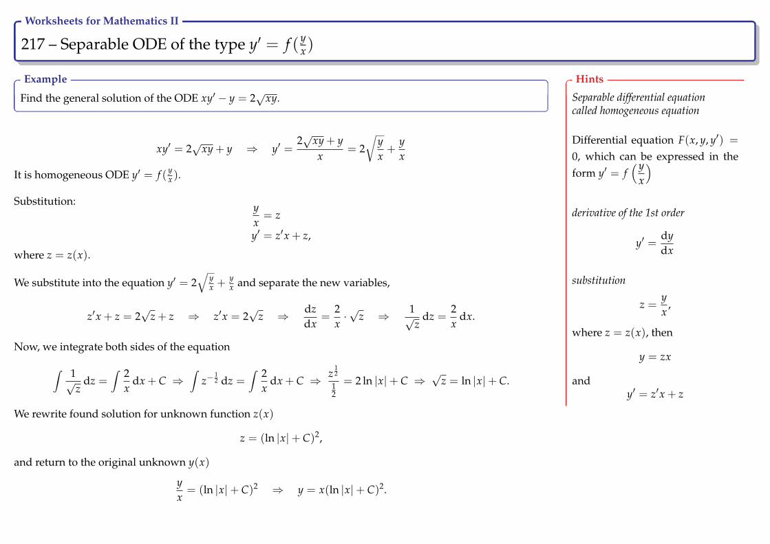
Worksheets for Mathematics II
217 – Separable ODE of the type y′ = f (yx) Ry
Example
Find the general solution of the ODE xy′ − y = 2√
xy.
xy′ = 2√
xy + y ⇒ y′ =2√
xy + yx
= 2√
yx+
yx
It is homogeneous ODE y′ = f ( yx ).
Substitution: yx= z
y′ = z′x + z,
where z = z(x).
We substitute into the equation y′ = 2√
yx + y
x and separate the new variables,
z′x + z = 2√
z + z ⇒ z′x = 2√
z ⇒ dzdx
=2x·√
z ⇒ 1√z
dz =2x
dx.
Now, we integrate both sides of the equation
∫ 1√z
dz =∫ 2
xdx + C ⇒
∫z−
12 dz =
∫ 2x
dx + C ⇒ z12
12
= 2 ln |x|+ C ⇒√
z = ln |x|+ C.
We rewrite found solution for unknown function z(x)
z = (ln |x|+ C)2,
and return to the original unknown y(x)
yx= (ln |x|+ C)2 ⇒ y = x(ln |x|+ C)2.
Hints
Separable differential equationcalled homogeneous equation
Differential equation F(x, y, y′) =
0, which can be expressed in theform y′ = f
(yx
)
derivative of the 1st order
y′ =dydx
substitution
z =yx
,
where z = z(x), then
y = zx
andy′ = z′x + z
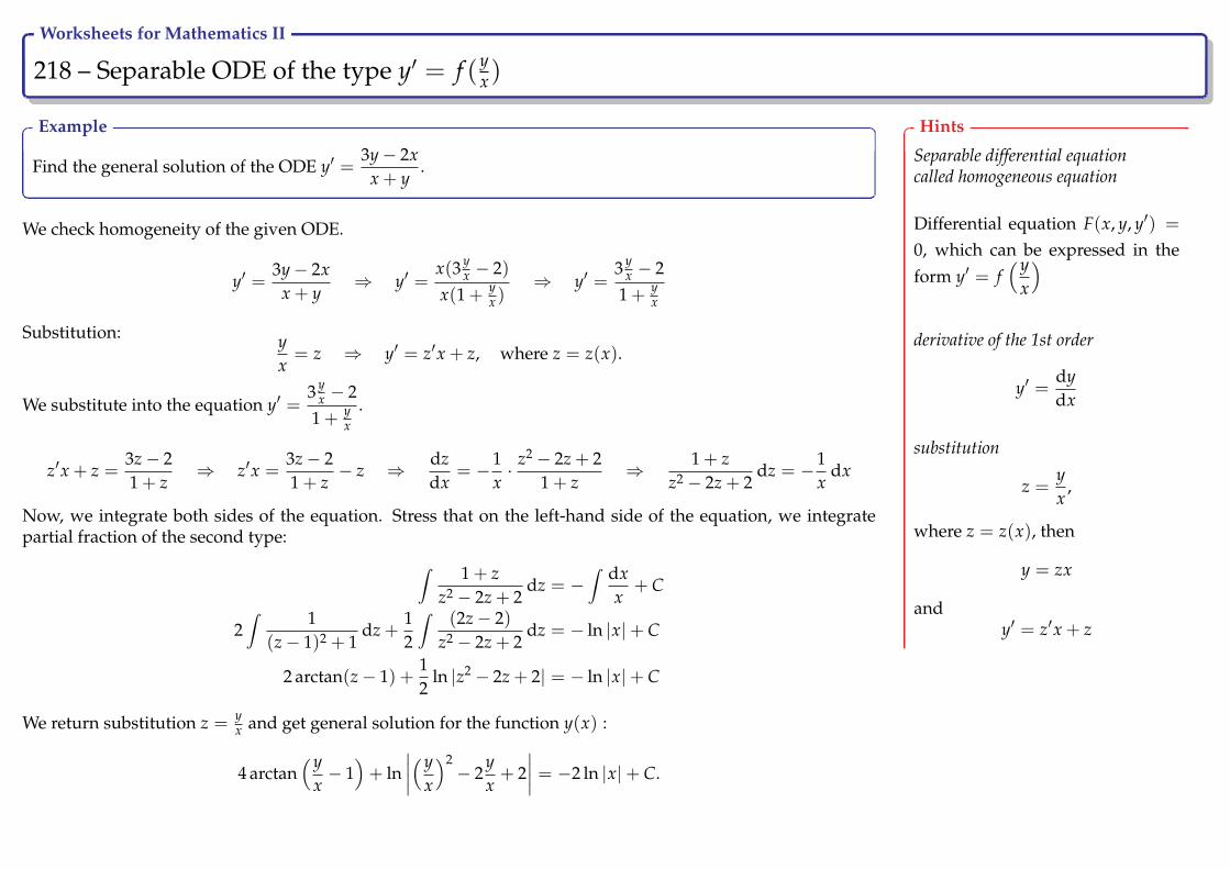
Worksheets for Mathematics II
218 – Separable ODE of the type y′ = f (yx) Ry
Example
Find the general solution of the ODE y′ =3y− 2x
x + y.
We check homogeneity of the given ODE.
y′ =3y− 2x
x + y⇒ y′ =
x(3 yx − 2)
x(1 + yx )
⇒ y′ =3 y
x − 21 + y
x
Substitution: yx= z ⇒ y′ = z′x + z, where z = z(x).
We substitute into the equation y′ =3 y
x − 21 + y
x.
z′x + z =3z− 21 + z
⇒ z′x =3z− 21 + z
− z ⇒ dzdx
= −1x· z2 − 2z + 2
1 + z⇒ 1 + z
z2 − 2z + 2dz = −1
xdx
Now, we integrate both sides of the equation. Stress that on the left-hand side of the equation, we integratepartial fraction of the second type: ∫ 1 + z
z2 − 2z + 2dz = −
∫ dxx
+ C
2∫ 1
(z− 1)2 + 1dz +
12
∫(2z− 2)
z2 − 2z + 2dz = − ln |x|+ C
2 arctan(z− 1) +12
ln |z2 − 2z + 2| = − ln |x|+ C
We return substitution z = yx and get general solution for the function y(x) :
4 arctan(y
x− 1)+ ln
∣∣∣∣(yx
)2− 2
yx+ 2∣∣∣∣ = −2 ln |x|+ C.
Hints
Separable differential equationcalled homogeneous equation
Differential equation F(x, y, y′) =
0, which can be expressed in theform y′ = f
(yx
)
derivative of the 1st order
y′ =dydx
substitution
z =yx
,
where z = z(x), then
y = zx
andy′ = z′x + z
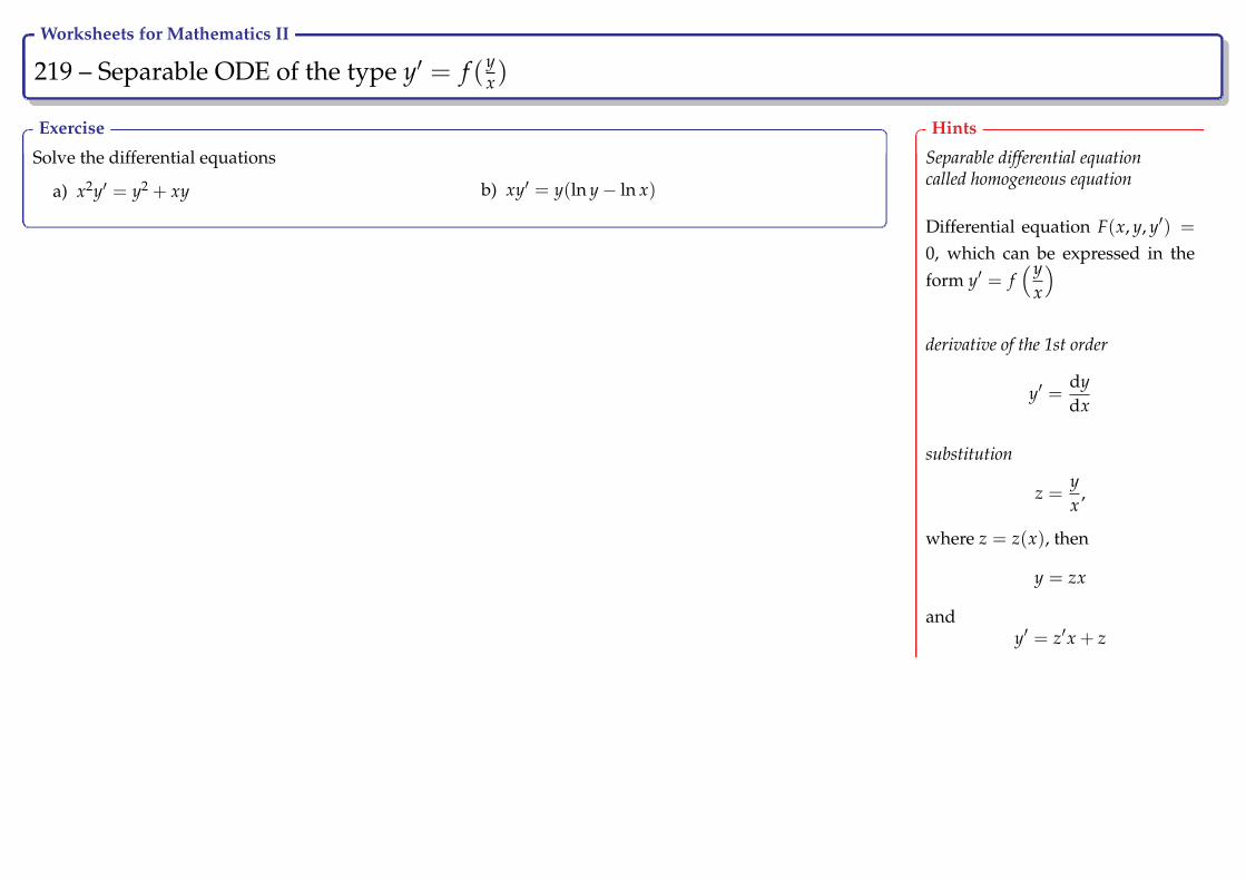
Worksheets for Mathematics II
219 – Separable ODE of the type y′ = f (yx) Ry
Exercise
Solve the differential equations
a) x2y′ = y2 + xy b) xy′ = y(ln y− ln x)
Hints
Separable differential equationcalled homogeneous equation
Differential equation F(x, y, y′) =
0, which can be expressed in theform y′ = f
(yx
)
derivative of the 1st order
y′ =dydx
substitution
z =yx
,
where z = z(x), then
y = zx
andy′ = z′x + z

Worksheets for Mathematics II
220 – Linear differential equations of the first order Ry
By linear differential equations we shall mean equations which are linearwith respect to an unknown function and its derivatives. Linear differen-tial equations are very important because a lot of practical problems canbe modelled by such equations.
Definition
We call linear ordinary differential equation (shortly LODE) of the firstorder every equation of the form
y′ + p(x)y = q(x),
where p(x), q(x) are continuous functions on some interval [a, b]. More-over,
• if q(x) = 0, we talk about homogeneous (shortened) LODE,
• if q(x) 6= 0, we talk about non-homogeneous (complete) LODE.
Remark
Examples of linear equations:
• xy′ − y = x
• y′ − ln x2 · y = sin x
• 2xy′ − yx− 2 = 0
Examples of non-linear equations:
• xy′y = x
• y′ − xy2 = sin x
• 2xy′ − xy− 2 sin y = 0
Homogeneous LODE y′+ p(x) · y = 0 is also separable ODE y′ = −p(x)y,which we know how to solve. To every complete LODE y′ + p(x)y = q(x)there exists associated shortened equation y′ + p(x)y = 0.
Theorem
Homogeneous LODE y′ + p(x)y = 0 has on the interval [a, b] generalsolution of the form
y = Ce−∫
p(x)dx, C ∈ R.
Theorem
General solution of complete LODE has the form
y(x) = y(x) + v(x),
where y(x) is general solution of associated homogeneous LODE andv(x) is a particular solution of the complete LODE.
The function v(x) is called particular integral of complete LODE.
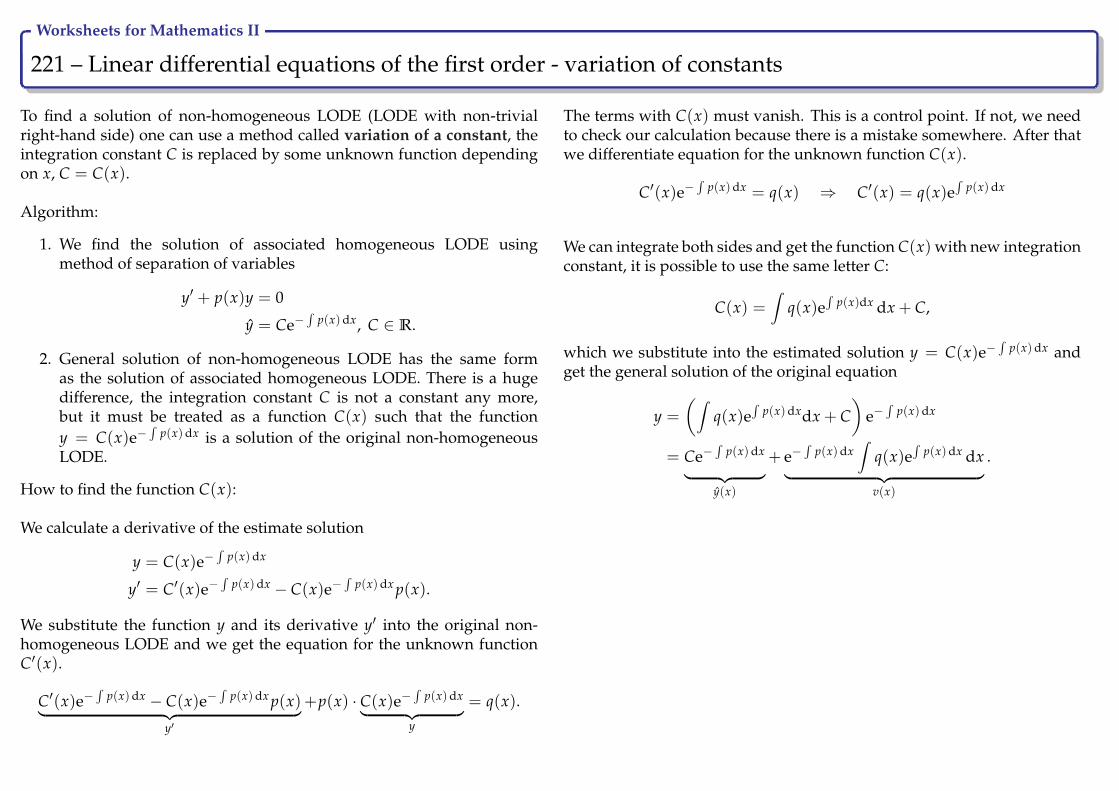
Worksheets for Mathematics II
221 – Linear differential equations of the first order - variation of constants Ry
To find a solution of non-homogeneous LODE (LODE with non-trivialright-hand side) one can use a method called variation of a constant, theintegration constant C is replaced by some unknown function dependingon x, C = C(x).
Algorithm:
1. We find the solution of associated homogeneous LODE usingmethod of separation of variables
y′ + p(x)y = 0
y = Ce−∫
p(x)dx, C ∈ R.
2. General solution of non-homogeneous LODE has the same formas the solution of associated homogeneous LODE. There is a hugedifference, the integration constant C is not a constant any more,but it must be treated as a function C(x) such that the functiony = C(x)e−
∫p(x)dx is a solution of the original non-homogeneous
LODE.
How to find the function C(x):
We calculate a derivative of the estimate solution
y = C(x)e−∫
p(x)dx
y′ = C′(x)e−∫
p(x)dx − C(x)e−∫
p(x)dx p(x).
We substitute the function y and its derivative y′ into the original non-homogeneous LODE and we get the equation for the unknown functionC′(x).
C′(x)e−∫
p(x)dx − C(x)e−∫
p(x)dx p(x)︸ ︷︷ ︸y′
+p(x) · C(x)e−∫
p(x)dx︸ ︷︷ ︸y
= q(x).
The terms with C(x) must vanish. This is a control point. If not, we needto check our calculation because there is a mistake somewhere. After thatwe differentiate equation for the unknown function C(x).
C′(x)e−∫
p(x)dx = q(x) ⇒ C′(x) = q(x)e∫
p(x)dx
We can integrate both sides and get the function C(x) with new integrationconstant, it is possible to use the same letter C:
C(x) =∫
q(x)e∫
p(x)dx dx + C,
which we substitute into the estimated solution y = C(x)e−∫
p(x)dx andget the general solution of the original equation
y =
(∫q(x)e
∫p(x)dxdx + C
)e−
∫p(x)dx
= Ce−∫
p(x)dx︸ ︷︷ ︸y(x)
+ e−∫
p(x)dx∫
q(x)e∫
p(x)dx dx︸ ︷︷ ︸v(x)
.

Worksheets for Mathematics II
222 – Linear differential equations of the first order Ry
Example
Find the general solution of LODE y′ − y = e2x.
Associated homogeneous LODE has the form y′ − y = 0. It is a separable ODE, thus
dydx
= y ⇒∫ dy
y=∫
dx + C ⇒ ln |y| = x + C ⇒ y = Cex.
We proceed with the variation of the integration constant. Assume that C = C(x), then
y = C(x)ex
and its derivative isy′ = C′(x)ex + C(x)ex.
After the substitution into the original ODE we get
C′(x)ex + C(x)ex − C(x)ex = e2x,
C′(x)ex = e2x ⇒ C′(x) = ex
We can directly integrate,
C(x) =∫
ex dx = ex + C.
After the substitution of y = C(x)ex into the general solution of homogeneous equation we get thegeneral solution of the original LODE
y = (ex + C) ex = Cex + e2x = y + v.
Hints
First order LODE y′ + p(x)y = q(x)
derivativey′ =
dydx
Algorithm
• we solve associated LODE
y′ + p(x)y = 0
by separation of variables
• Variation of constantC = C(x) is substituted into the generalsolution of homogeneous LODE, then thesolution is differentiated and put into theoriginal LODE
• control point: the terms containing C(x)must vanish (yes - correct, not - mistakein calculations)
• we calculate C′(x), integrate it and put itinto the general solution
• result:
y =1
E(x)
(∫E(x)q(x)dx + K
),
where E(x) = e∫
p(x)dx
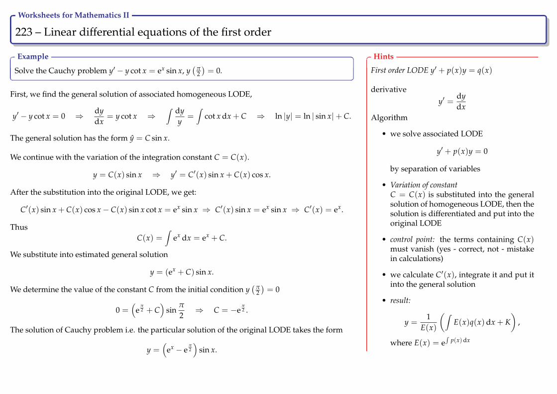
Worksheets for Mathematics II
223 – Linear differential equations of the first order Ry
Example
Solve the Cauchy problem y′ − y cot x = ex sin x, y(
π2
)= 0.
First, we find the general solution of associated homogeneous LODE,
y′ − y cot x = 0 ⇒ dydx
= y cot x ⇒∫ dy
y=∫
cot x dx + C ⇒ ln |y| = ln | sin x|+ C.
The general solution has the form y = C sin x.
We continue with the variation of the integration constant C = C(x).
y = C(x) sin x ⇒ y′ = C′(x) sin x + C(x) cos x.
After the substitution into the original LODE, we get:
C′(x) sin x + C(x) cos x− C(x) sin x cot x = ex sin x ⇒ C′(x) sin x = ex sin x ⇒ C′(x) = ex.
ThusC(x) =
∫ex dx = ex + C.
We substitute into estimated general solution
y = (ex + C) sin x.
We determine the value of the constant C from the initial condition y(
π2
)= 0
0 =(
eπ2 + C
)sin
π
2⇒ C = −e
π2 .
The solution of Cauchy problem i.e. the particular solution of the original LODE takes the form
y =(
ex − eπ2
)sin x.
Hints
First order LODE y′ + p(x)y = q(x)
derivativey′ =
dydx
Algorithm
• we solve associated LODE
y′ + p(x)y = 0
by separation of variables
• Variation of constantC = C(x) is substituted into the generalsolution of homogeneous LODE, then thesolution is differentiated and put into theoriginal LODE
• control point: the terms containing C(x)must vanish (yes - correct, not - mistakein calculations)
• we calculate C′(x), integrate it and put itinto the general solution
• result:
y =1
E(x)
(∫E(x)q(x)dx + K
),
where E(x) = e∫
p(x)dx
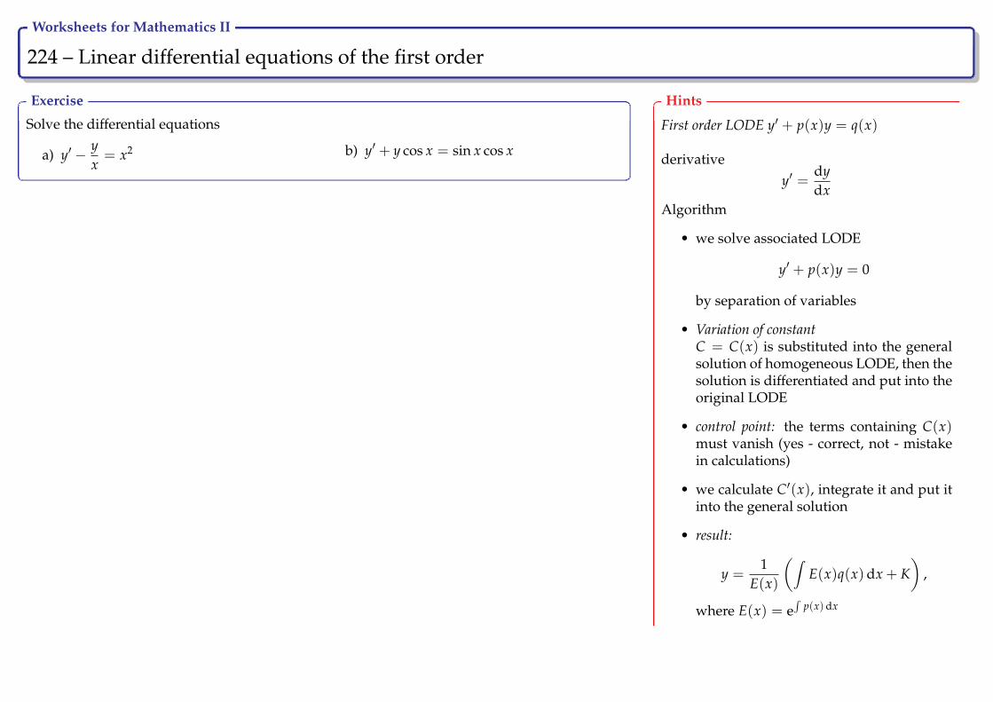
Worksheets for Mathematics II
224 – Linear differential equations of the first order Ry
Exercise
Solve the differential equations
a) y′ − yx= x2 b) y′ + y cos x = sin x cos x
Hints
First order LODE y′ + p(x)y = q(x)
derivativey′ =
dydx
Algorithm
• we solve associated LODE
y′ + p(x)y = 0
by separation of variables
• Variation of constantC = C(x) is substituted into the generalsolution of homogeneous LODE, then thesolution is differentiated and put into theoriginal LODE
• control point: the terms containing C(x)must vanish (yes - correct, not - mistakein calculations)
• we calculate C′(x), integrate it and put itinto the general solution
• result:
y =1
E(x)
(∫E(x)q(x)dx + K
),
where E(x) = e∫
p(x)dx

Worksheets for Mathematics II
225 – Linear differential equations of the first order Ry
Exercise
Solve the Cauchy problems
a) y′ − ysin xcos x
=1
cos x, y(0) = 0 b) xy′ − y
x + 1= x, y(1) = 0
Hints
First order LODE y′ + p(x)y = q(x)
derivativey′ =
dydx
Algorithm
• we solve associated LODE
y′ + p(x)y = 0
by separation of variables
• Variation of constantC = C(x) is substituted into the generalsolution of homogeneous LODE, then thesolution is differentiated and put into theoriginal LODE
• control point: the terms containing C(x)must vanish (yes - correct, not - mistakein calculations)
• we calculate C′(x), integrate it and put itinto the general solution
• result:
y =1
E(x)
(∫E(x)q(x)dx + K
),
where E(x) = e∫
p(x)dx
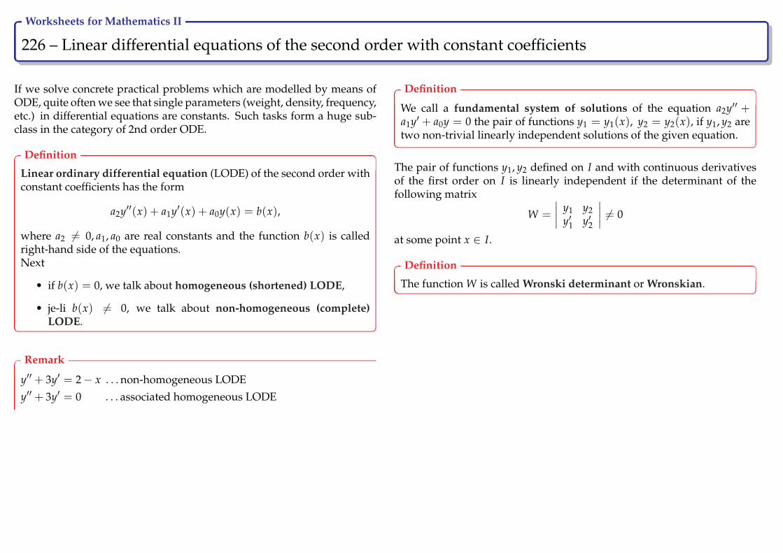
Worksheets for Mathematics II
226 – Linear differential equations of the second order with constant coefficients Ry
If we solve concrete practical problems which are modelled by means ofODE, quite often we see that single parameters (weight, density, frequency,etc.) in differential equations are constants. Such tasks form a huge sub-class in the category of 2nd order ODE.
Definition
Linear ordinary differential equation (LODE) of the second order withconstant coefficients has the form
a2y′′(x) + a1y′(x) + a0y(x) = b(x),
where a2 6= 0, a1, a0 are real constants and the function b(x) is calledright-hand side of the equations.Next
• if b(x) = 0, we talk about homogeneous (shortened) LODE,
• je-li b(x) 6= 0, we talk about non-homogeneous (complete)LODE.
Remark
y′′ + 3y′ = 2− x . . . non-homogeneous LODE
y′′ + 3y′ = 0 . . . associated homogeneous LODE
Definition
We call a fundamental system of solutions of the equation a2y′′ +a1y′ + a0y = 0 the pair of functions y1 = y1(x), y2 = y2(x), if y1, y2 aretwo non-trivial linearly independent solutions of the given equation.
The pair of functions y1, y2 defined on I and with continuous derivativesof the first order on I is linearly independent if the determinant of thefollowing matrix
W =
∣∣∣∣ y1 y2y′1 y′2
∣∣∣∣ 6= 0
at some point x ∈ I.
Definition
The function W is called Wronski determinant or Wronskian.

Worksheets for Mathematics II
227 – Linearly independent functions Ry
Example
Show that the functions y1 = e3x, y2 = xe3x are linearly independent on R.
We calculate the Wronskian:
W =
∣∣∣∣ e3x xe3x
3e3x e3x + 3xe3x
∣∣∣∣ = e3x(e3x + 3xe3x)− 3xe6x = e6x.
Because e6x 6= 0 for ∀x ∈ R, the functions y1 = e3x, y2 = xe3x are linearly independent on R.
Hints
If
W =
∣∣∣∣ y1 y2y′1 y′2
∣∣∣∣ 6= 0,
at some point x ∈ I, then the func-tions y1, y2 are linearly indepen-dent on I.
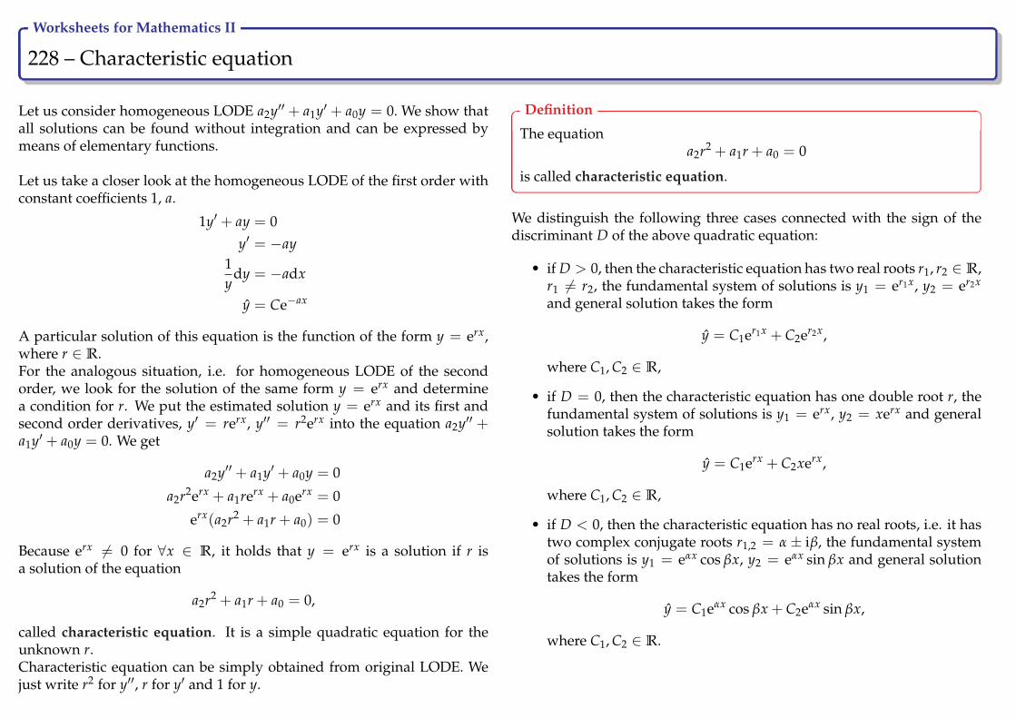
Worksheets for Mathematics II
228 – Characteristic equation Ry
Let us consider homogeneous LODE a2y′′ + a1y′ + a0y = 0. We show thatall solutions can be found without integration and can be expressed bymeans of elementary functions.
Let us take a closer look at the homogeneous LODE of the first order withconstant coefficients 1, a.
1y′ + ay = 0
y′ = −ay1y
dy = −adx
y = Ce−ax
A particular solution of this equation is the function of the form y = erx,where r ∈ R.For the analogous situation, i.e. for homogeneous LODE of the secondorder, we look for the solution of the same form y = erx and determinea condition for r. We put the estimated solution y = erx and its first andsecond order derivatives, y′ = rerx, y′′ = r2erx into the equation a2y′′ +a1y′ + a0y = 0. We get
a2y′′ + a1y′ + a0y = 0
a2r2erx + a1rerx + a0erx = 0
erx(a2r2 + a1r + a0) = 0
Because erx 6= 0 for ∀x ∈ R, it holds that y = erx is a solution if r isa solution of the equation
a2r2 + a1r + a0 = 0,
called characteristic equation. It is a simple quadratic equation for theunknown r.Characteristic equation can be simply obtained from original LODE. Wejust write r2 for y′′, r for y′ and 1 for y.
Definition
The equationa2r2 + a1r + a0 = 0
is called characteristic equation.
We distinguish the following three cases connected with the sign of thediscriminant D of the above quadratic equation:
• if D > 0, then the characteristic equation has two real roots r1, r2 ∈ R,r1 6= r2, the fundamental system of solutions is y1 = er1x, y2 = er2x
and general solution takes the form
y = C1er1x + C2er2x,
where C1, C2 ∈ R,
• if D = 0, then the characteristic equation has one double root r, thefundamental system of solutions is y1 = erx, y2 = xerx and generalsolution takes the form
y = C1erx + C2xerx,
where C1, C2 ∈ R,
• if D < 0, then the characteristic equation has no real roots, i.e. it hastwo complex conjugate roots r1,2 = α± iβ, the fundamental systemof solutions is y1 = eαx cos βx, y2 = eαx sin βx and general solutiontakes the form
y = C1eαx cos βx + C2eαx sin βx,
where C1, C2 ∈ R.
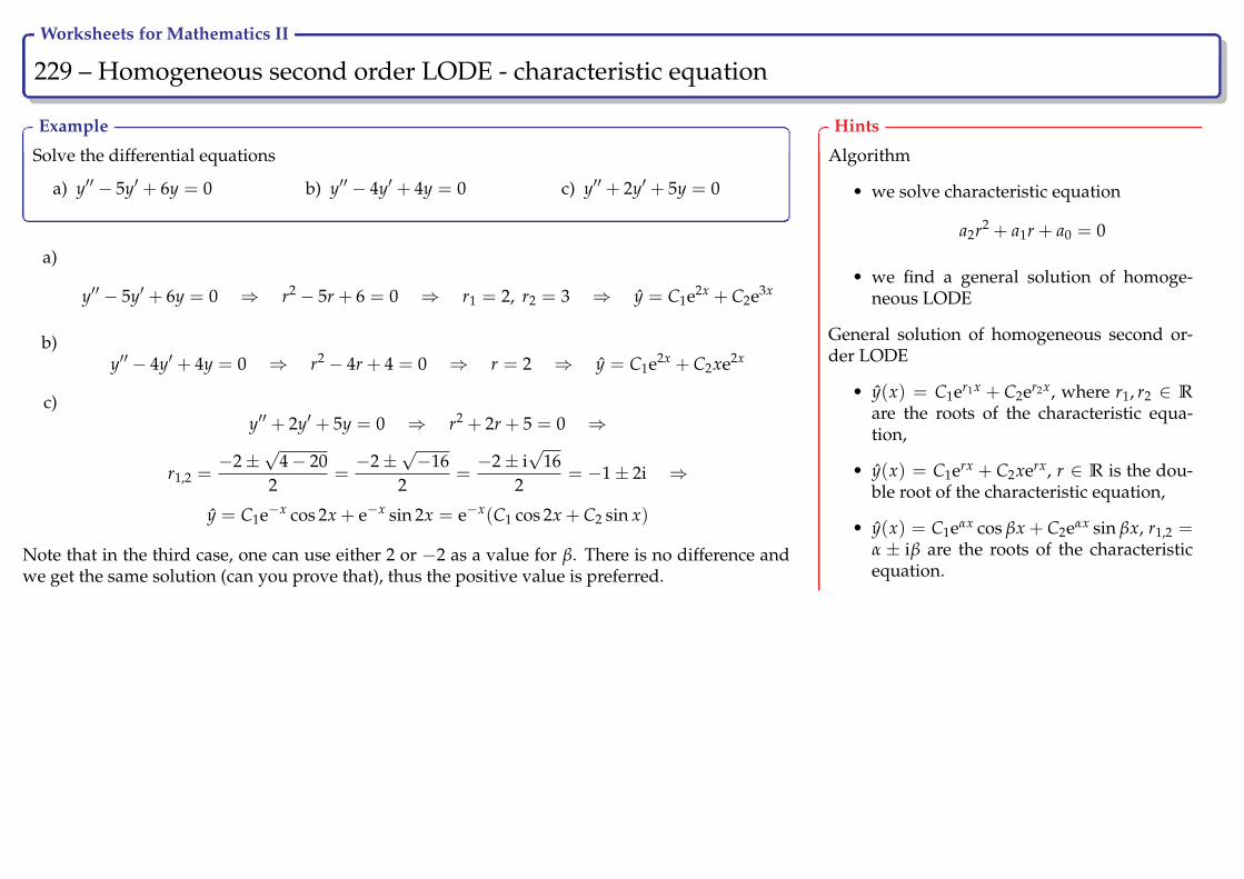
Worksheets for Mathematics II
229 – Homogeneous second order LODE - characteristic equation Ry
Example
Solve the differential equations
a) y′′ − 5y′ + 6y = 0 b) y′′ − 4y′ + 4y = 0 c) y′′ + 2y′ + 5y = 0
a)
y′′ − 5y′ + 6y = 0 ⇒ r2 − 5r + 6 = 0 ⇒ r1 = 2, r2 = 3 ⇒ y = C1e2x + C2e3x
b)y′′ − 4y′ + 4y = 0 ⇒ r2 − 4r + 4 = 0 ⇒ r = 2 ⇒ y = C1e2x + C2xe2x
c)y′′ + 2y′ + 5y = 0 ⇒ r2 + 2r + 5 = 0 ⇒
r1,2 =−2±
√4− 20
2=−2±
√−16
2=−2± i
√16
2= −1± 2i ⇒
y = C1e−x cos 2x + e−x sin 2x = e−x(C1 cos 2x + C2 sin x)
Note that in the third case, one can use either 2 or −2 as a value for β. There is no difference andwe get the same solution (can you prove that), thus the positive value is preferred.
Hints
Algorithm
• we solve characteristic equation
a2r2 + a1r + a0 = 0
• we find a general solution of homoge-neous LODE
General solution of homogeneous second or-der LODE
• y(x) = C1er1x + C2er2x, where r1, r2 ∈ R
are the roots of the characteristic equa-tion,
• y(x) = C1erx + C2xerx, r ∈ R is the dou-ble root of the characteristic equation,
• y(x) = C1eαx cos βx + C2eαx sin βx, r1,2 =α ± iβ are the roots of the characteristicequation.
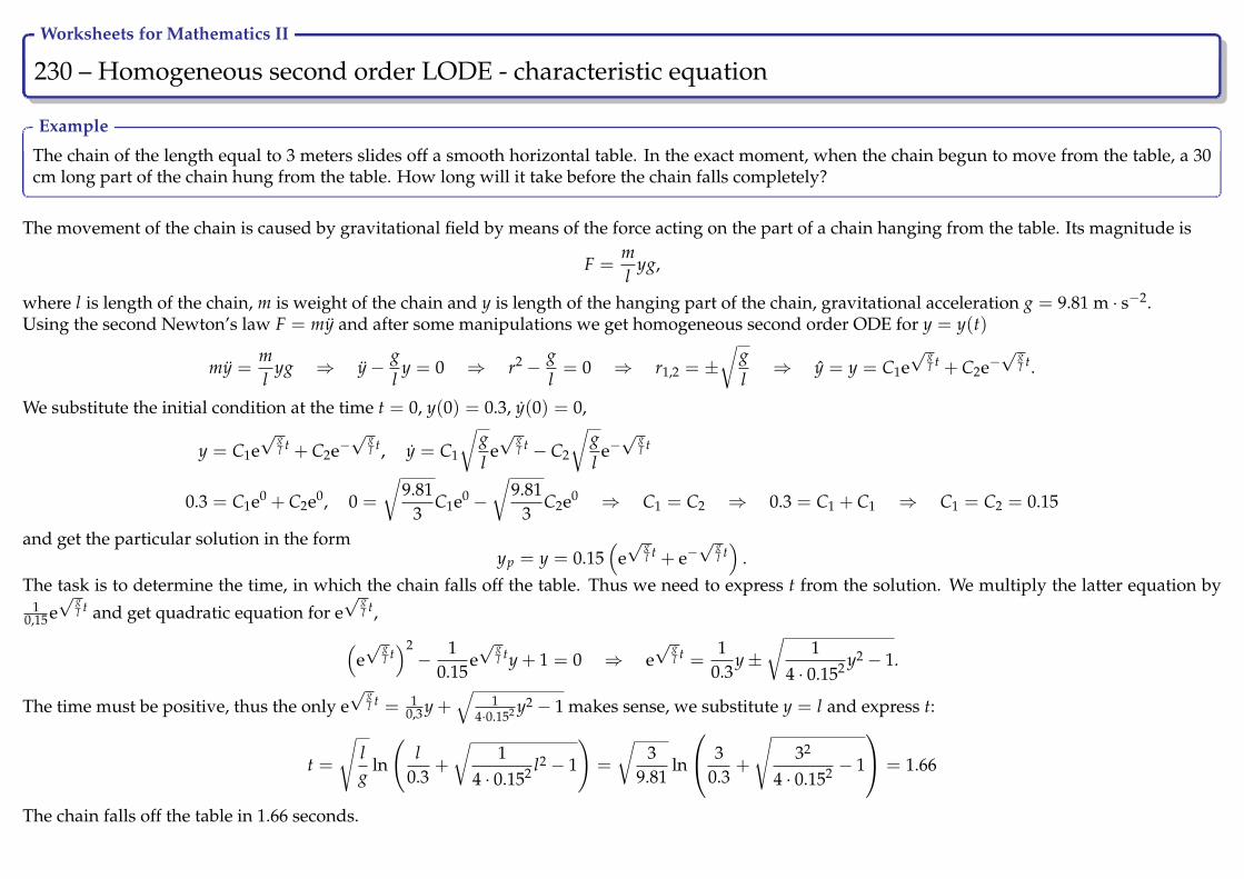
Worksheets for Mathematics II
230 – Homogeneous second order LODE - characteristic equation Ry
Example
The chain of the length equal to 3 meters slides off a smooth horizontal table. In the exact moment, when the chain begun to move from the table, a 30cm long part of the chain hung from the table. How long will it take before the chain falls completely?
The movement of the chain is caused by gravitational field by means of the force acting on the part of a chain hanging from the table. Its magnitude is
F =ml
yg,
where l is length of the chain, m is weight of the chain and y is length of the hanging part of the chain, gravitational acceleration g = 9.81 m · s−2.Using the second Newton’s law F = my and after some manipulations we get homogeneous second order ODE for y = y(t)
my =ml
yg ⇒ y− gl
y = 0 ⇒ r2 − gl= 0 ⇒ r1,2 = ±
√gl⇒ y = y = C1e
√ gl t + C2e−
√ gl t.
We substitute the initial condition at the time t = 0, y(0) = 0.3, y(0) = 0,
y = C1e√ g
l t + C2e−√ g
l t, y = C1
√gl
e√ g
l t − C2
√gl
e−√ g
l t
0.3 = C1e0 + C2e0, 0 =
√9.81
3C1e0 −
√9.81
3C2e0 ⇒ C1 = C2 ⇒ 0.3 = C1 + C1 ⇒ C1 = C2 = 0.15
and get the particular solution in the formyp = y = 0.15
(e√ g
l t + e−√ g
l t)
.The task is to determine the time, in which the chain falls off the table. Thus we need to express t from the solution. We multiply the latter equation by
10,15e√ g
l t and get quadratic equation for e√ g
l t,(e√ g
l t)2− 1
0.15e√ g
l ty + 1 = 0 ⇒ e√ g
l t =1
0.3y±
√1
4 · 0.152 y2 − 1.
The time must be positive, thus the only e√ g
l t = 10,3 y +
√1
4·0.152 y2 − 1 makes sense, we substitute y = l and express t:
t =
√lg
ln
(l
0.3+
√1
4 · 0.152 l2 − 1
)=
√3
9.81ln
30.3
+
√32
4 · 0.152 − 1
= 1.66
The chain falls off the table in 1.66 seconds.
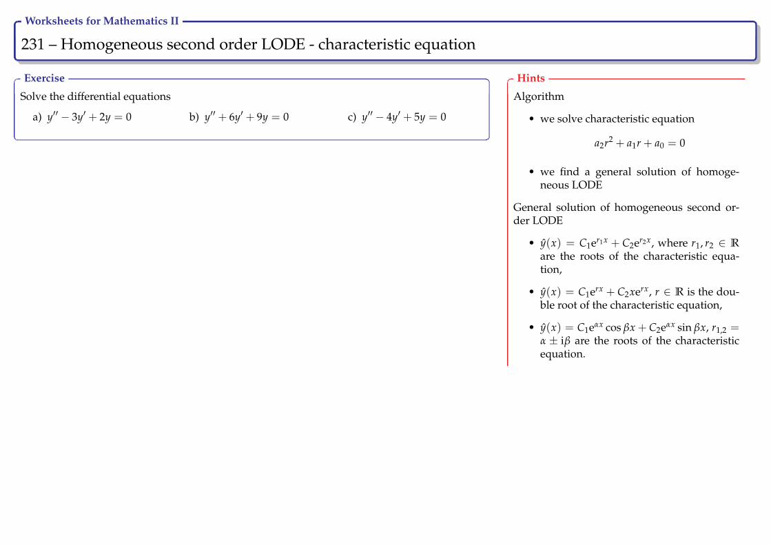
Worksheets for Mathematics II
231 – Homogeneous second order LODE - characteristic equation Ry
Exercise
Solve the differential equations
a) y′′ − 3y′ + 2y = 0 b) y′′ + 6y′ + 9y = 0 c) y′′ − 4y′ + 5y = 0
Hints
Algorithm
• we solve characteristic equation
a2r2 + a1r + a0 = 0
• we find a general solution of homoge-neous LODE
General solution of homogeneous second or-der LODE
• y(x) = C1er1x + C2er2x, where r1, r2 ∈ R
are the roots of the characteristic equa-tion,
• y(x) = C1erx + C2xerx, r ∈ R is the dou-ble root of the characteristic equation,
• y(x) = C1eαx cos βx + C2eαx sin βx, r1,2 =α ± iβ are the roots of the characteristicequation.
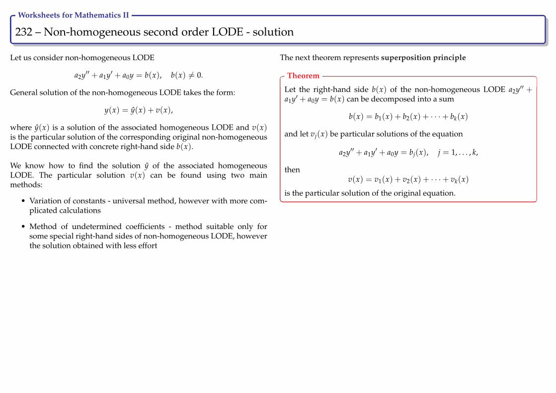
Worksheets for Mathematics II
232 – Non-homogeneous second order LODE - solution Ry
Let us consider non-homogeneous LODE
a2y′′ + a1y′ + a0y = b(x), b(x) 6= 0.
General solution of the non-homogeneous LODE takes the form:
y(x) = y(x) + v(x),
where y(x) is a solution of the associated homogeneous LODE and v(x)is the particular solution of the corresponding original non-homogeneousLODE connected with concrete right-hand side b(x).
We know how to find the solution y of the associated homogeneousLODE. The particular solution v(x) can be found using two mainmethods:
• Variation of constants - universal method, however with more com-plicated calculations
• Method of undetermined coefficients - method suitable only forsome special right-hand sides of non-homogeneous LODE, howeverthe solution obtained with less effort
The next theorem represents superposition principle
Theorem
Let the right-hand side b(x) of the non-homogeneous LODE a2y′′ +a1y′ + a0y = b(x) can be decomposed into a sum
b(x) = b1(x) + b2(x) + · · ·+ bk(x)
and let vj(x) be particular solutions of the equation
a2y′′ + a1y′ + a0y = bj(x), j = 1, . . . , k,
thenv(x) = v1(x) + v2(x) + · · ·+ vk(x)
is the particular solution of the original equation.

Worksheets for Mathematics II
233 – Variation of constants 1/2 Ry
The core of the method is the same as in the case of the 1st order LODE.The next theorem characterizes Variation of constants for 2nd orderLODE.
Theorem
General solution of the equation
a2y′′ + a1y′ + a0y = b(x)
with constant coefficient a2, a1, a0 one can express in the form
y(x) = y(x) + v(x) = y(x) + y1(x)∫ W1(x)
W(x)dx + y2(x)
∫ W2(x)W(x)
dx,
where y(x) = C1y1(x) + C2y2(x) is the general solution of associatedhomogeneous LODE, W(x) is Wronskian of its fundamental system andW1(x), W2(x) are determinants which come from Wronskian W(x) byreplacing its first respectively second column by the vector of right-hand side (0, b(x)/a2).
We solve the non-homogeneous 2nd order LODE with constant coeffi-cients
a2y′′ + a1y′ + a0y = b(x)
under the assumption that we know solutions of associated homogeneousLODE y = C1y1(x) + C2y2(x).
Let us assume that general solution of non-homogeneous 2nd orderLODE will have the same form as the solution of homogeneous LODE,however we replace integration constants C1, C2 by unknown functionsC1(x), C2(x). We make variation of constants. We seek the solution in theform
y(x) = C1(x)y1(x) + C2(x)y2(x).
We calculate derivative of the estimated solution
y′ = C′1y1 + C1y′1 + C′2y2 + C2y′2.
The choice of the new functions C1(x), C2(x) allows us to set up a suitableadditional condition,
C′1y1 + C′2y2 = 0.
Substituting the condition into the first derivative we get
y′ = C1y′1 + C2y′2 and y′′ = C′1y′1 + C1y′′1 + C′2y′2 + C2y′′2 ,
which we put into the original non-homogeneous LODE
a2(C′1y′1 + C1y′′1 + C′2y′2 + C2y′′2︸ ︷︷ ︸y′′
)+ a1(C1y′1 + C2y′2︸ ︷︷ ︸y′
)+ a0(C1y1 + C2y2︸ ︷︷ ︸y
) = b(x)
and get
C1(a2y′′1 + a1y′1 + a0y1) +C2(a2y′′2 + a1y′2 + a0y2) + a2(C′1y′1 +C′2y′2) = b(x).
Because the functions y1, y2 are solutions of the associated homogeneousLODE, the expression in brackets must be null, and we get
C′1y′1 + C′2y′2 =b(x)
a2.
Thereby, we obtained second condition for derivatives of unknown func-tions C1(x), C2(x) and we solve the following system of linear equationsfor the unknowns C′1, C′2,
C′1y1 + C′2y2 = 0,
C′1y′1 + C′2y′2 =b(x)
a2.

Worksheets for Mathematics II
234 – Variation of constants 2/2 Ry
The determinant of the system is the Wronskian of the functions y1, y2
W =
∣∣∣∣y1 y2y′1 y′2
∣∣∣∣ ,
which is not null because both functions are linearly independent, they form fundamental systemof solutions. The system has just one solution which can be found by the help of Cramer’s rule
C′1(x) =W1(x)W(x)
, C′2(x) =W2(x)W(x)
,
where
W1 =
∣∣∣∣∣ 0 y2b(x)a2
y′2
∣∣∣∣∣ and W2 =
∣∣∣∣∣y1 0y′1
b(x)a2
∣∣∣∣∣ .
After integration we get
C1(x) =∫ W1(x)
W(x)dx + K1, C2(x) =
∫ W2(x)W(x)
dx + K2,
where K1, K2 ∈ R. If we substitute into the estimated solution y(x) = C1(x)y1(x) + C2(x)y2(x) weget general solution of non-homogeneous LODE in the form
y(x) = y(x) + v(x) = K1y1(x) + K2y2(x)︸ ︷︷ ︸y(x)
+y1(x)∫ W1(x)
W(x)dx + y2(x)
∫ W2(x)W(x)
dx︸ ︷︷ ︸v(x)
.
Finally, one can use the same letters C for the integrations constants, thus
y(x) = y(x) + v(x) = C1y1(x) + C2y2(x)︸ ︷︷ ︸y(x)
+y1(x)∫ W1(x)
W(x)dx + y2(x)
∫ W2(x)W(x)
dx︸ ︷︷ ︸v(x)
.
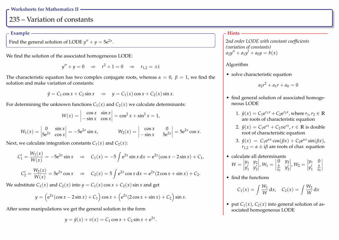
Worksheets for Mathematics II
235 – Variation of constants Ry
Example
Find the general solution of LODE y′′ + y = 5e2x.
We find the solution of the associated homogeneous LODE:
y′′ + y = 0 ⇒ r2 + 1 = 0 ⇒ r1,2 = ±i
The characteristic equation has two complex conjugate roots, whereas α = 0, β = 1, we find thesolution and make variation of constants:
y = C1 cos x + C2 sin x ⇒ y = C1(x) cos x + C2(x) sin x.
For determining the unknown functions C1(x) and C2(x) we calculate determinants:
W(x) =∣∣∣∣ cos x sin x− sin x cos x
∣∣∣∣ = cos2 x + sin2 x = 1,
W1(x) =∣∣∣∣ 0 sin x5e2x cos x
∣∣∣∣ = −5e2x sin x, W2(x) =∣∣∣∣ cos x 0− sin x 5e2x
∣∣∣∣ = 5e2x cos x.
Next, we calculate integration constants C1(x) and C2(x):
C′1 =W1(x)W(x)
= −5e2x sin x ⇒ C1(x) = −5∫
e2x sin x dx = e2x(cos x− 2 sin x) + C1,
C′2 =W2(x)W(x)
= 5e2x cos x ⇒ C2(x) = 5∫
e2x cos x dx = e2x(2 cos x + sin x) + C2.
We substitute C1(x) and C2(x) into y = C1(x) cos x + C2(x) sin x and get
y =(
e2x(cos x− 2 sin x) + C1
)cos x +
(e2x(2 cos x + sin x) + C2
)sin x.
After some manipulations we get the general solution in the form
y = y(x) + v(x) = C1 cos x + C2 sin x + e2x.
Hints
2nd order LODE with constant coefficients(variation of constants)a2y′′ + a1y′ + a0y = b(x)
Algorithm
• solve characteristic equation
a2r2 + a1r + a0 = 0
• find general solution of associated homoge-neous LODE
1. y(x) = C1er1x +C2er2x, where r1, r2 ∈ R
are roots of characteristic equation
2. y(x) = C1erx + C2xerx, r ∈ R is doubleroot of characteristic equation
3. y(x) = C1eαx cos(βx) + C2eαx sin(βx),r1,2 = α± iβ are roots of char. equation
• calculate all determinants
W =
∣∣∣∣y1 y2y′1 y′2
∣∣∣∣, W1 =
∣∣∣∣ 0 y2ba2
y′2
∣∣∣∣, W2 =
∣∣∣∣y1 0y′1
ba2
∣∣∣∣• find the functions
C1(x) =∫ W1
Wdx, C2(x) =
∫ W2
Wdx
• put C1(x), C2(x) into general solution of as-sociated homogeneous LODE

Worksheets for Mathematics II
236 – Variation of constants Ry
Example
Find the general solution of LODE y′′ + 3y′ + 2y =1
1 + ex .
We find the solution of associated homogeneous LODE:
y′′ + 3y′ + 2y = 0 ⇒ r2 + 3r + 2 = 0 ⇒ r1 = −1, r2 = −2
The characteristic eq. has two different real roots, we find the solution and make variation ofconstants:
y = C1e−x + C2e−2x ⇒ y = C1(x)e−x + C2(x)e−2x.
For determining unknown functions C1(x) and C2(x) we calculate determinants
W(x) =∣∣∣∣ e−x e−2x
−e−x −2e−2x
∣∣∣∣ = −2e−3x + e−3x = −e−3x,
W1(x) =∣∣∣∣ 0 e−2x
11+ex −2e−2x
∣∣∣∣ = − e−2x
1 + ex , W2(x) =∣∣∣∣ e−x 0−e−x 1
1+ex
∣∣∣∣ = e−x
1 + ex .
Next, we calculate integration constants C1(x) and C2(x):
C′1 =W1(x)W(x)
= − e−2x
(1 + ex)(−e−3x)=
ex
1 + ex ⇒ C1(x) =∫ ex
1 + ex dx = ln |1 + ex|+ C1,
C′2 =W2(x)W(x)
=e−x
(1 + ex)(−e−3x)= − e2x
1 + ex ⇒ C2(x) = −∫ e2x
1 + ex dx = ln |1 + ex| − ex + C2.
We substitute C1(x) and C2(x) into y = C1(x)e−x + C2(x)e−2x and get
y = (ln |1 + ex|+ C1) e−x + (ln |1 + ex| − ex + C2) e−2x.
After some manipulations we get the general solution in the form
y = y(x) + v(x) = C1e−x + C2e−2x + e−x ln |1 + ex|+ e−2x(ln |1 + ex| − ex).
Hints
2nd order LODE with constant coefficients(variation of constants)a2y′′ + a1y′ + a0y = b(x)
Algorithm
• solve characteristic equation
a2r2 + a1r + a0 = 0
• find general solution of associated homoge-neous LODE
1. y(x) = C1er1x +C2er2x, where r1, r2 ∈ R
are roots of characteristic equation
2. y(x) = C1erx + C2xerx, r ∈ R is doubleroot of characteristic equation
3. y(x) = C1eαx cos(βx) + C2eαx sin(βx),r1,2 = α± iβ are roots of char. equation
• calculate all determinants
W =
∣∣∣∣y1 y2y′1 y′2
∣∣∣∣, W1 =
∣∣∣∣ 0 y2ba2
y′2
∣∣∣∣, W2 =
∣∣∣∣y1 0y′1
ba2
∣∣∣∣• find the functions
C1(x) =∫ W1
Wdx, C2(x) =
∫ W2
Wdx
• put C1(x), C2(x) into general solution of as-sociated homogeneous LODE

Worksheets for Mathematics II
237 – Variation of constants Ry
Exercise
Solve the differential equation y′′ − 5y′ + 6y = 6x2 − 10x− 4.
Hints
2nd order LODE with constant coefficients(variation of constants)a2y′′ + a1y′ + a0y = b(x)
Algorithm
• solve characteristic equation
a2r2 + a1r + a0 = 0
• find general solution of associated homoge-neous LODE
1. y(x) = C1er1x +C2er2x, where r1, r2 ∈ R
are roots of characteristic equation
2. y(x) = C1erx + C2xerx, r ∈ R is doubleroot of characteristic equation
3. y(x) = C1eαx cos(βx) + C2eαx sin(βx),r1,2 = α± iβ are roots of char. equation
• calculate all determinants
W =
∣∣∣∣y1 y2y′1 y′2
∣∣∣∣, W1 =
∣∣∣∣ 0 y2ba2
y′2
∣∣∣∣, W2 =
∣∣∣∣y1 0y′1
ba2
∣∣∣∣• find the functions
C1(x) =∫ W1
Wdx, C2(x) =
∫ W2
Wdx
• put C1(x), C2(x) into general solution of as-sociated homogeneous LODE
Worksheets for Mathematics II
238 – Variation of constants Ry
Exercise
Solve the differential equation y′′ − 4y′ = 4 sin x− cos x.
Hints
2nd order LODE with constant coefficients(variation of constants)a2y′′ + a1y′ + a0y = b(x)
Algorithm
• solve characteristic equation
a2r2 + a1r + a0 = 0
• find general solution of associated homoge-neous LODE
1. y(x) = C1er1x +C2er2x, where r1, r2 ∈ R
are roots of characteristic equation
2. y(x) = C1erx + C2xerx, r ∈ R is doubleroot of characteristic equation
3. y(x) = C1eαx cos(βx) + C2eαx sin(βx),r1,2 = α± iβ are roots of char. equation
• calculate all determinants
W =
∣∣∣∣y1 y2y′1 y′2
∣∣∣∣, W1 =
∣∣∣∣ 0 y2ba2
y′2
∣∣∣∣, W2 =
∣∣∣∣y1 0y′1
ba2
∣∣∣∣• find the functions
C1(x) =∫ W1
Wdx, C2(x) =
∫ W2
Wdx
• put C1(x), C2(x) into general solution of as-sociated homogeneous LODE
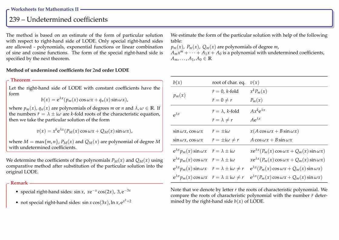
Worksheets for Mathematics II
239 – Undetermined coefficients Ry
The method is based on an estimate of the form of particular solutionwith respect to right-hand side of LODE. Only special right-hand sidesare allowed - polynomials, exponential functions or linear combinationof sine and cosine functions. The form of the special right-hand side isspecified by the next theorem.
Method of undermined coefficients for 2nd order LODE
Theorem
Let the right-hand side of LODE with constant coefficients have theform
b(x) = eλx(pm(x) cos ωx + qn(x) sin ωx),
where pm(x), qn(x) are polynomials of degrees m or n and λ, ω ∈ R. Ifthe numbers r = λ± iω are k-fold roots of the characteristic equation,then we take the particular solution of the form
v(x) = xkeλx(PM(x) cos ωx + QM(x) sin ωx),
where M = maxm, n, PM(x) and QM(x) are polynomial of degree Mwith undetermined coefficients.
We determine the coefficients of the polynomials PM(x) and QM(x) usingcomparative method after substitution of the particular solution into theoriginal LODE.
Remark
• special right-hand sides: sin x, xe−x cos(2x), 3, e−3x
• not special right-hand sides: sin x cos(3x), ln x, ex2+2
We estimate the form of the particular solution with help of the followingtable:pm(x), Pm(x), Qm(x) are polynomials of degree m,Amxm + · · ·+ A1x + A0 is a polynomial with undetermined coefficients,Am, . . . , A1, A0 ∈ R
b(x) root of char. eq. v(x)
pm(x)r = 0, k-fold xkPm(x)
r = 0 6= r Pm(x)
eλx r = λ, k-fold Axkeλx
r = λ 6= r Aeλx
sin ωx, cos ωx r = ±iω x(A cos ωx + B sin ωx)
sin ωx, cos ωx r = ±iω 6= r A cos ωx + B sin ωx
eλx pm(x) sin ωx r = λ± iω xeλx(Pm(x) cos ωx + Qm(x) sin ωx)
eλx pm(x) cos ωx r = λ± iω xeλx(Pm(x) cos ωx + Qm(x) sin ωx)
eλx pm(x) sin ωx r = λ± iω 6= r eλx(Pm(x) cos ωx + Qm(x) sin ωx)
eλx pm(x) cos ωx r = λ± iω 6= r eλx(Pm(x) cos ωx + Qm(x) sin ωx)
Note that we denote by letter r the roots of characteristic polynomial. Wecompare the roots of characteristic polynomial with the number r deter-mined by the right-hand side b(x) of LODE.

Worksheets for Mathematics II
240 – Undetermined coefficients Ry
Example
Try to estimate the form of a particular solution of the differential equa-tion y′′ + 5y′ = b(x):
a) b(x) = 5x2,
b) b(x) = sin(5x),
c) b(x) = 3e5x,
d) b(x) = 3xe−5x,
e) b(x) = e−x cos 2x,
f) b(x) = ex + 2.
We find the roots of the characteristic equation:
y′′ + 5y′ = 0 ⇒ r2 + 5r = 0 ⇒ r1 = 0, r2 = −5
a)b(x) = 5x2 ⇒ λ = 0, ω = 0 ⇒ r = 0,
but r = 0 is simple root of the characteristic equation, thus we needto add factor x to the estimated form of the particular solution, whichis a polynomial of 2nd degree with undetermined coefficients
v(x) = x(Ax2 + Bx + C)
b)b(x) = sin 5x ⇒ λ = 0, ω = 5 ⇒ r = ±i5,
but neither r = i5 nor r = −i5 are roots of the characteristic equation,thus the particular solution takes the form
v(x) = A cos 5x + B sin 5x
c)b(x) = 3e5x ⇒ λ = 5, ω = 0 ⇒ r = 5,
but r = 5 is not the root of the characteristic equation,
v(x) = Ae5x
d)b(x) = 3xe−5x ⇒ λ = −5, ω = 0 ⇒ r = −5,
but r = −5 is simple root of the characteristic equation, we need toadd factor x, thus
v(x) = x(Ax + B)e−5x
e)
b(x) = e−x cos 2x ⇒ λ = −1, ω = 2 ⇒ r = −1± i2,
but r are not the roots of the characteristic equation,
v(x) = e−x(A cos 2x + B sin 2x)
f)b(x) = ex + 2
it is not special right-hand side because there is addition betweenexponential and constant. Right-hand side can be considered as ad-dition of two functions, each of which has the form of a special right-hand side, one can use superposition principle
v(x) = v1(x) + v2(x),
where v1(x) relates b1(x) = ex and v2(x) relates b2(x) = 2
v1(x) = Aex, r = 1 is not the root of the characteristic equa-tionv2(x) = Bx, r = 0 is simple root of the characteristic equation
v(x) = Aex + Bx
To find unknown coefficients we need to substitute estimated particularsolution into original non-homogeneous LODE.

Worksheets for Mathematics II
241 – Undetermined coefficients Ry
Example
Solve LODE y′′ + 4y = −2.
We find the solution of associated homogeneous equation:
y′′ + 4y = 0,
r2 + 4 = 0,r1,2 = ±2i.
The characteristic equation has two complex conjugate roots, whereas α = 0, β = 2, thus thesolution takes the form:
y = C1 cos 2x + C2 sin 2x.
b(x) = −2 - special right-hand side ⇒ we use the method of undermined coefficients, λ = 0,ω = 0,⇒ r = λ± iω = 0, but r = 0 is not the root of the characteristic equation
Particular solution takes the form: v(x) = A.
We calculate the first and second order derivatives: v′ = 0, v′′ = 0, and substitute theminto y′′ + 4y = −2 and get:
0 + 4A = −2 ⇒ A = −12
.
Particular solution:v = −1
2.
General solution y = y(x) + v(x):
y = y(x) + v(x) = C1 cos 2x + C2 sin 2x− 12
.
Hints
2nd order LODE with constant coefficients(variation of constants)a2y′′ + a1y′ + a0y = b(x)
Algorithm
• solve the characteristic equation
a2r2 + a1r + a0 = 0
• find the general solution of associated ho-mogeneous LODE
1. y(x) = C1er1x + C2er2x, where r1, r2 ∈R are roots of characteristic equation
2. y(x) = C1erx + C2xerx, r ∈ R is doubleroot of characteristic equation
3. y(x) = C1eαx cos(βx) + C2eαx sin(βx),r1,2 = α± iβ are roots of char. equation
• with respect to RHS of LODEb(x) = eλx (pm(x) cos(ωx) + qn(x) sin(ωx)),and if r = λ± iω is k-fold root of the char-acteristic eq. we choose particular solutionv(x) = xkeλx (PM(x) cos(ωx)+QM(x) sin(ωx)) , where M = maxm, n
• we differentiate v(x), we substitute it intooriginal LODE and finally we calculate co-efficients
• general solution of LODE of the 2nd ordery(x) = y(x) + v(x)

Worksheets for Mathematics II
242 – Undetermined coefficients Ry
Example
Solve LODE y′′ − 10y′ + 24y = (3x− 1)e3x.
We find the solution of associated homogeneous equation:
y′′ − 10y′ + 24y = 0 ⇒ r2 − 10r + 24 = 0 ⇒ r1 = 4, r2 = 6,
thus the solution takes the formy = C1e4x + C2e6x.
b(x) = (3x − 1)e3x - special right-hand side ⇒ we use the method of undetermined coefficients,λ = 3, ω = 0⇒ r = λ± iω = 3, but r = 3 is not the root of the characteristic equation
Particular solution: v(x) = (Ax + B)e3x.
Derivatives:v′ = Ae3x + 3(Ax + B)e3x, v′′ = 6Ae3x + 9e3x(Ax + B).
We substitute the estimated particular solution and its derivatives into original LODE
6Ae3x + 9e3x(Ax + B)︸ ︷︷ ︸v′′
−10(
Ae3x + 3(Ax + B)e3x)
︸ ︷︷ ︸v′
+24 (Ax + B) e3x︸ ︷︷ ︸v(x)
= (3x− 1)e3x,
and after some manipulations we get
3Axe3x + (−4A + 3B)e3x = 3xe3x − e3x.
We compare coefficients of the expressions xe3x and e3x on both sides of the equation
xe3x : 3A = 3e3x : −4A + 3B = −1
⇒ A = 1 and B = 1.
Particular solutionv(x) = (x + 1) e3x.
General solutiony = y(x) + v(x) = C1e4x + C2e6x + (x + 1) e3x.
Hints
2nd order LODE with constant coefficients(variation of constants)a2y′′ + a1y′ + a0y = b(x)
Algorithm
• solve the characteristic equation
a2r2 + a1r + a0 = 0
• find the general solution of associated ho-mogeneous LODE
1. y(x) = C1er1x + C2er2x, where r1, r2 ∈R are roots of characteristic equation
2. y(x) = C1erx + C2xerx, r ∈ R is doubleroot of characteristic equation
3. y(x) = C1eαx cos(βx) + C2eαx sin(βx),r1,2 = α± iβ are roots of char. equation
• with respect to RHS of LODEb(x) = eλx (pm(x) cos(ωx) + qn(x) sin(ωx)),and if r = λ± iω is k-fold root of the char-acteristic eq. we choose particular solutionv(x) = xkeλx (PM(x) cos(ωx)+QM(x) sin(ωx)) , where M = maxm, n
• we differentiate v(x), we substitute it intooriginal LODE and finally we calculate co-efficients
• general solution of LODE of the 2nd ordery(x) = y(x) + v(x)

Worksheets for Mathematics II
243 – Undetermined coefficients Ry
Example
Solve LODE y′′ − 2y′ + 2y = ex sin x.
We find the solution of associated homogeneous equation:
y′′ − 2y′ + 2y = 0 ⇒ r2 − 2r + 2 = 0 ⇒ r1,2 = 1± i,
thus the solution takes the form
y(x) = C1ex cos x + C2ex sin x.
b(x) = ex sin x - special right-hand side⇒ we use the method of undetermined coefficients, λ = 1,ω = 1⇒ r = λ± iω = 1± i, but r = 1± i are simple roots of the characteristic equation
Particular solution: v(x) = xex (A sin x + B cos x).
Derivativesv′ = ex(A sin x + B cos x) + xex(A sin x + B cos x) + xex(A cos x− B sin x),v′′ = 2ex ((A + B + Bx) cos x− (A− B + Ax) sin x) .
We substitute the estimated solution and its derivatives into original LODE
2ex ((A + B + Bx) cos x− (A− B + Ax) sin x)− 2ex(A sin x + B cos x + x(A sin x+B cos x + A cos x− B sin x)) + 2xex (A sin x + B cos x) = ex sin x,
and after some manipulations we get
2B cos x− 2A sin x = sin x.
We compare coefficients of the expressions cos x and sin x on both sides of the equation
cos x : 2B = 0sin x : −2A = 1
⇒ A = −1
2 and B = 0.
Particular solutionv(x) = −1
2xex sin x.
General solutiony = y(x) + v(x) = C1ex cos x + C2ex sin x− 1
2xex sin x.
Hints
2nd order LODE with constant coefficients(variation of constants)a2y′′ + a1y′ + a0y = b(x)
Algorithm
• solve the characteristic equation
a2r2 + a1r + a0 = 0
• find the general solution of associated ho-mogeneous LODE
1. y(x) = C1er1x + C2er2x, where r1, r2 ∈R are roots of characteristic equation
2. y(x) = C1erx + C2xerx, r ∈ R is doubleroot of characteristic equation
3. y(x) = C1eαx cos(βx) + C2eαx sin(βx),r1,2 = α± iβ are roots of char. equation
• with respect to RHS of LODEb(x) = eλx (pm(x) cos(ωx) + qn(x) sin(ωx)),and if r = λ± iω is k-fold root of the char-acteristic eq. we choose particular solutionv(x) = xkeλx (PM(x) cos(ωx)+QM(x) sin(ωx)) , where M = maxm, n
• we differentiate v(x), we substitute it intooriginal LODE and finally we calculate co-efficients
• general solution of LODE of the 2nd ordery(x) = y(x) + v(x)
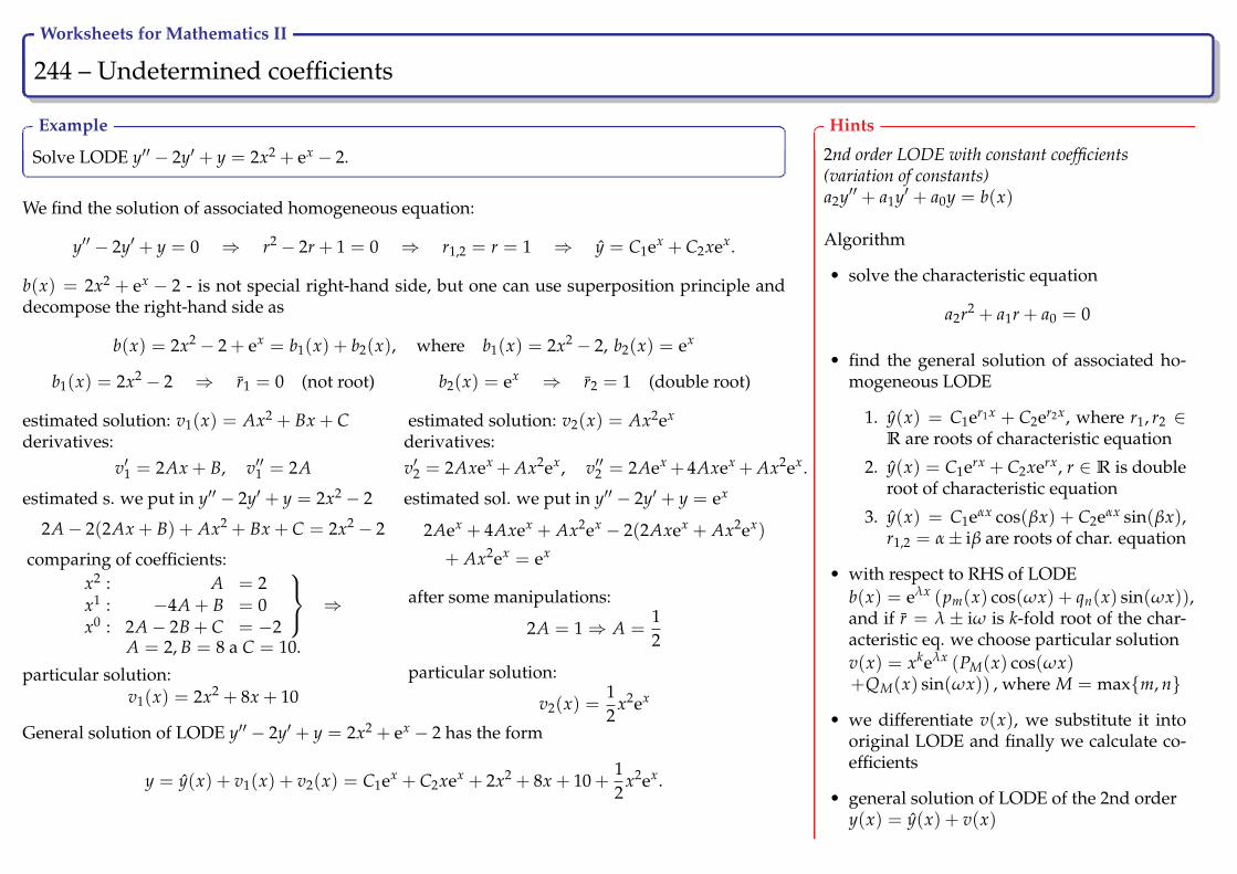
Worksheets for Mathematics II
244 – Undetermined coefficients Ry
Example
Solve LODE y′′ − 2y′ + y = 2x2 + ex − 2.
We find the solution of associated homogeneous equation:
y′′ − 2y′ + y = 0 ⇒ r2 − 2r + 1 = 0 ⇒ r1,2 = r = 1 ⇒ y = C1ex + C2xex.
b(x) = 2x2 + ex − 2 - is not special right-hand side, but one can use superposition principle anddecompose the right-hand side as
b(x) = 2x2 − 2 + ex = b1(x) + b2(x), where b1(x) = 2x2 − 2, b2(x) = ex
b1(x) = 2x2 − 2 ⇒ r1 = 0 (not root)
estimated solution: v1(x) = Ax2 + Bx + Cderivatives:
v′1 = 2Ax + B, v′′1 = 2A
estimated s. we put in y′′ − 2y′ + y = 2x2 − 2
2A− 2(2Ax + B) + Ax2 + Bx + C = 2x2 − 2
comparing of coefficients:x2 : A = 2x1 : −4A + B = 0x0 : 2A− 2B + C = −2
⇒
A = 2, B = 8 a C = 10.
particular solution:v1(x) = 2x2 + 8x + 10
b2(x) = ex ⇒ r2 = 1 (double root)
estimated solution: v2(x) = Ax2ex
derivatives:v′2 = 2Axex + Ax2ex, v′′2 = 2Aex + 4Axex + Ax2ex.
estimated sol. we put in y′′ − 2y′ + y = ex
2Aex + 4Axex + Ax2ex − 2(2Axex + Ax2ex)
+ Ax2ex = ex
after some manipulations:
2A = 1⇒ A =12
particular solution:
v2(x) =12
x2ex
General solution of LODE y′′ − 2y′ + y = 2x2 + ex − 2 has the form
y = y(x) + v1(x) + v2(x) = C1ex + C2xex + 2x2 + 8x + 10 +12
x2ex.
Hints
2nd order LODE with constant coefficients(variation of constants)a2y′′ + a1y′ + a0y = b(x)
Algorithm
• solve the characteristic equation
a2r2 + a1r + a0 = 0
• find the general solution of associated ho-mogeneous LODE
1. y(x) = C1er1x + C2er2x, where r1, r2 ∈R are roots of characteristic equation
2. y(x) = C1erx + C2xerx, r ∈ R is doubleroot of characteristic equation
3. y(x) = C1eαx cos(βx) + C2eαx sin(βx),r1,2 = α± iβ are roots of char. equation
• with respect to RHS of LODEb(x) = eλx (pm(x) cos(ωx) + qn(x) sin(ωx)),and if r = λ± iω is k-fold root of the char-acteristic eq. we choose particular solutionv(x) = xkeλx (PM(x) cos(ωx)+QM(x) sin(ωx)) , where M = maxm, n
• we differentiate v(x), we substitute it intooriginal LODE and finally we calculate co-efficients
• general solution of LODE of the 2nd ordery(x) = y(x) + v(x)

Worksheets for Mathematics II
245 – Undetermined coefficients Ry
Exercise
Solve LODE
a) y′′ − 2y′ = x3 + 2x b) y′′ − 3y′ − 4y = 3e2x
Hints
2nd order LODE with constant coefficients(variation of constants)a2y′′ + a1y′ + a0y = b(x)
Algorithm
• solve the characteristic equation
a2r2 + a1r + a0 = 0
• find the general solution of associated ho-mogeneous LODE
1. y(x) = C1er1x + C2er2x, where r1, r2 ∈R are roots of characteristic equation
2. y(x) = C1erx + C2xerx, r ∈ R is doubleroot of characteristic equation
3. y(x) = C1eαx cos(βx) + C2eαx sin(βx),r1,2 = α± iβ are roots of char. equation
• with respect to RHS of LODEb(x) = eλx (pm(x) cos(ωx) + qn(x) sin(ωx)),and if r = λ± iω is k-fold root of the char-acteristic eq. we choose particular solutionv(x) = xkeλx (PM(x) cos(ωx)+QM(x) sin(ωx)) , where M = maxm, n
• we differentiate v(x), we substitute it intooriginal LODE and finally we calculate co-efficients
• general solution of LODE of the 2nd ordery(x) = y(x) + v(x)

Worksheets for Mathematics II
246 – Undetermined coefficients Ry
Exercise
Solve LODE
a) y′′ + y′ − 2y = 2x b) y′′ + 2y′ = 8 cos 4x
Hints
2nd order LODE with constant coefficients(variation of constants)a2y′′ + a1y′ + a0y = b(x)
Algorithm
• solve the characteristic equation
a2r2 + a1r + a0 = 0
• find the general solution of associated ho-mogeneous LODE
1. y(x) = C1er1x + C2er2x, where r1, r2 ∈R are roots of characteristic equation
2. y(x) = C1erx + C2xerx, r ∈ R is doubleroot of characteristic equation
3. y(x) = C1eαx cos(βx) + C2eαx sin(βx),r1,2 = α± iβ are roots of char. equation
• with respect to RHS of LODEb(x) = eλx (pm(x) cos(ωx) + qn(x) sin(ωx)),and if r = λ± iω is k-fold root of the char-acteristic eq. we choose particular solutionv(x) = xkeλx (PM(x) cos(ωx)+QM(x) sin(ωx)) , where M = maxm, n
• we differentiate v(x), we substitute it intooriginal LODE and finally we calculate co-efficients
• general solution of LODE of the 2nd ordery(x) = y(x) + v(x)

Worksheets for Mathematics II
247 – Undetermined coefficients Ry
Exercise
Solve LODE
a) y′′ − 2y′ + 10y = 12ex cos 3x b) y′′ − 5y′ + 4y = ex sin x
Hints
2nd order LODE with constant coefficients(variation of constants)a2y′′ + a1y′ + a0y = b(x)
Algorithm
• solve the characteristic equation
a2r2 + a1r + a0 = 0
• find the general solution of associated ho-mogeneous LODE
1. y(x) = C1er1x + C2er2x, where r1, r2 ∈R are roots of characteristic equation
2. y(x) = C1erx + C2xerx, r ∈ R is doubleroot of characteristic equation
3. y(x) = C1eαx cos(βx) + C2eαx sin(βx),r1,2 = α± iβ are roots of char. equation
• with respect to RHS of LODEb(x) = eλx (pm(x) cos(ωx) + qn(x) sin(ωx)),and if r = λ± iω is k-fold root of the char-acteristic eq. we choose particular solutionv(x) = xkeλx (PM(x) cos(ωx)+QM(x) sin(ωx)) , where M = maxm, n
• we differentiate v(x), we substitute it intooriginal LODE and finally we calculate co-efficients
• general solution of LODE of the 2nd ordery(x) = y(x) + v(x)

Worksheets for Mathematics II
248 – Undetermined coefficients Ry
Exercise
Solve LODE
a) y′′ − 3y′ − 10y = 2(7x + 1)e5x b) y′′ − 5y′ + 6y = 6x2 − 10x− 4
Hints
2nd order LODE with constant coefficients(variation of constants)a2y′′ + a1y′ + a0y = b(x)
Algorithm
• solve the characteristic equation
a2r2 + a1r + a0 = 0
• find the general solution of associated ho-mogeneous LODE
1. y(x) = C1er1x + C2er2x, where r1, r2 ∈R are roots of characteristic equation
2. y(x) = C1erx + C2xerx, r ∈ R is doubleroot of characteristic equation
3. y(x) = C1eαx cos(βx) + C2eαx sin(βx),r1,2 = α± iβ are roots of char. equation
• with respect to RHS of LODEb(x) = eλx (pm(x) cos(ωx) + qn(x) sin(ωx)),and if r = λ± iω is k-fold root of the char-acteristic eq. we choose particular solutionv(x) = xkeλx (PM(x) cos(ωx)+QM(x) sin(ωx)) , where M = maxm, n
• we differentiate v(x), we substitute it intooriginal LODE and finally we calculate co-efficients
• general solution of LODE of the 2nd ordery(x) = y(x) + v(x)

Worksheets for Mathematics II
249 – Undetermined coefficients Ry
Exercise
Solve LODE y′′ − 4y′ = 4 sin x− cos x.
Hints
2nd order LODE with constant coefficients(variation of constants)a2y′′ + a1y′ + a0y = b(x)
Algorithm
• solve the characteristic equation
a2r2 + a1r + a0 = 0
• find the general solution of associated ho-mogeneous LODE
1. y(x) = C1er1x + C2er2x, where r1, r2 ∈R are roots of characteristic equation
2. y(x) = C1erx + C2xerx, r ∈ R is doubleroot of characteristic equation
3. y(x) = C1eαx cos(βx) + C2eαx sin(βx),r1,2 = α± iβ are roots of char. equation
• with respect to RHS of LODEb(x) = eλx (pm(x) cos(ωx) + qn(x) sin(ωx)),and if r = λ± iω is k-fold root of the char-acteristic eq. we choose particular solutionv(x) = xkeλx (PM(x) cos(ωx)+QM(x) sin(ωx)) , where M = maxm, n
• we differentiate v(x), we substitute it intooriginal LODE and finally we calculate co-efficients
• general solution of LODE of the 2nd ordery(x) = y(x) + v(x)
Worksheets for Mathematics II
250 – Undetermined coefficients Ry
Exercise
Solve Cauchy problem y′′ + 9y = 8 cos x, y(
π3
)= 0, y′
(π3
)= −
√3
2 .
Hints
2nd order LODE with constant coefficients(variation of constants)a2y′′ + a1y′ + a0y = b(x)
Algorithm
• solve the characteristic equation
a2r2 + a1r + a0 = 0
• find the general solution of associated ho-mogeneous LODE
1. y(x) = C1er1x + C2er2x, where r1, r2 ∈R are roots of characteristic equation
2. y(x) = C1erx + C2xerx, r ∈ R is doubleroot of characteristic equation
3. y(x) = C1eαx cos(βx) + C2eαx sin(βx),r1,2 = α± iβ are roots of char. equation
• with respect to RHS of LODEb(x) = eλx (pm(x) cos(ωx) + qn(x) sin(ωx)),and if r = λ± iω is k-fold root of the char-acteristic eq. we choose particular solutionv(x) = xkeλx (PM(x) cos(ωx)+QM(x) sin(ωx)) , where M = maxm, n
• we differentiate v(x), we substitute it intooriginal LODE and finally we calculate co-efficients
• general solution of LODE of the 2nd ordery(x) = y(x) + v(x)
Name: Worksheets for Mathematics II
Department, Institute: Faculty of Civil Engineering, Department of Mathematics
Authors: Jana Volná, Petr Volný
Place, year of publishing: Ostrava, 2021, 1st Edition
Number of Pages: 251
Published: VSB – Technical University of Ostrava