working with data lesson 7. objectives software orientation: excel’s data tab the command groups...
TRANSCRIPT

Working with DataLesson 7

Objectives
Software Orientation: Excel’s Data Tab
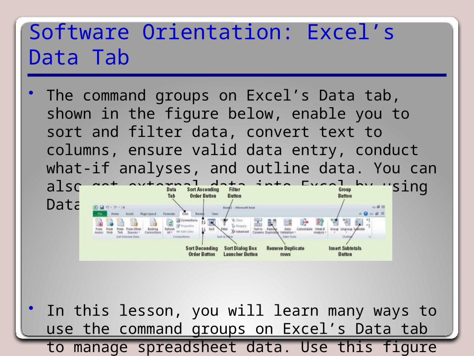
• The command groups on Excel’s Data tab, shown in the figure below, enable you to sort and filter data, convert text to columns, ensure valid data entry, conduct what-if analyses, and outline data. You can also get external data into Excel by using Data commands.
• In this lesson, you will learn many ways to use the command groups on Excel’s Data tab to manage spreadsheet data. Use this figure as a guide to these powerful commands.

Ensuring Your Data’s Integrity
• Ensuring valid data entry is an important task for Excel users. In many worksheets that you create, other users may enter data to get desired calculations and results.
• Restricting the type of data that can be entered in a cell is one way to ensure data integrity. You may want to restrict data entry to a certain range of dates, limit choices by using a drop-down list, or make sure that only positive whole numbers are entered.
• And, because it’s not uncommon for users to inadvertently enter duplicate rows of information in lengthy spreadsheets, you need to have a mechanism for finding and eliminating duplicate information.

Restricting Cell Entries to Certain Data Types
• When you decide what data type you want to use in a cell or range of cells and how you want it used, formatted, or displayed, you are ready to set up the validation criteria for that data.
• Data Validation is the feature in Excel that will manage data that is to be entered or displayed based on your specified criteria.
• When you restrict (validate) data entry, it is necessary to provide immediate feedback to instruct users about the data that is permitted in a cell. This feedback is on the form of alerts and error messages that you create.

Restricting Cell Entries to Certain Data Types
• You can provide an input message when a restricted cell is selected or provide an instructive message when an invalid entry is made.
• In the next exercise, you learn how to validate data and restrict data entry while supplying clear feedback to users to assure a smooth, trouble-free data entry experience. This is vital to worksheet performance because it restricts errors in data entry.

Restricting Cell Entries to Certain Data Types
• After completing the next exercise, you will take the first step toward ensuring the integrity of data entered in the Contoso Data workbook.
• An employee cannot inadvertently enter text or values that are outside the parameters you set in the validation criteria.
• By extending the range beyond the current data, when new employee data is entered, the validation criteria will be applied.

Restricting Cell Entries to Certain Data Types
• You can specify how you want Excel to respond when invalid data is entered. In the next exercise, you accept the default value, Stop, in the Style box on the Error Alert tab (see the figure on slide 11).
• If you select Warning in the Style box, you will be warned that you have made an entry that is not in the defined range, but you can choose to ignore the warning and enter the invalid data.
Step-by-Step: Restrict Cell Entries to Data Types
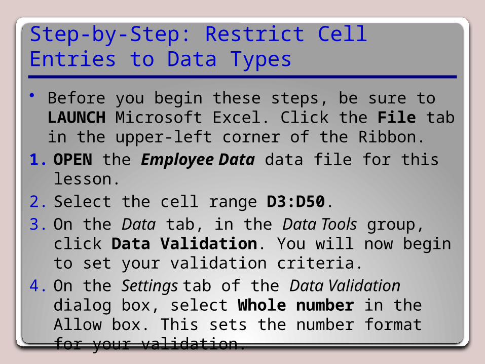
• Before you begin these steps, be sure to LAUNCH Microsoft Excel. Click the File tab in the upper-left corner of the Ribbon.
1. OPEN the Employee Data data file for this lesson.
2. Select the cell range D3:D50.3. On the Data tab, in the Data Tools group, click
Data Validation. You will now begin to set your validation criteria.
4. On the Settings tab of the Data Validation dialog box, select Whole number in the Allow box. This sets the number format for your validation.
Step-by-Step: Restrict Cell Entries to Data Types
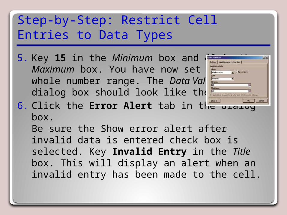
5. Key 15 in the Minimum box and 40 in the Maximum box. You have now set your whole number range. The Data Validation dialog box should look like the figure.
6. Click the Error Alert tab in the dialog box. Be sure the Show error alert after invalid data is entered check box is selected. Key Invalid Entry in the Title box. This will display an alert when an invalid entry has been made to the cell.

Step-by-Step: Restrict Cell Entries to Data Types
7. Key Only whole numbers can be entered in the error message box as shown in the figure. This will display the error message that you want the user to see.
8. Click the Input Message tab and in the Input Message box, key Enter a whole number between 15 and 40. Click OK. This will create the message for the user to follow to correct their error.

Step-by-Step: Restrict Cell Entries to Data Types
9. Select cell D6, key 35.5, and press Enter. The Invalid Entry dialog box (see the figure) opens, displaying the error message you created.
10.Click Retry to close the error message; key 36, and press Enter.
11.Use the following employee information to key values in row 29. Patricia Doyle was hired today as a receptionist. She will work 20 hours each week.
12.Create a Lesson 7 folder and SAVE the file as Contoso Data.
• LEAVE the workbook open to use in the next exercise.

Allowing Specific Values to Be Entered in Cells
• To make data entry easier, or to limit entries to predefined items, you can create a drop-down list of valid entries.
• The entries on the list can be forced-choice (i.e., yes, no) or can be compiled from cells elsewhere in the workbook.
• A drop-down list displays as an arrow in the cell. • To enter information in the restricted cell, click
the arrow and then click the entry you want.

Allowing Specific Values to Be Entered in Cells
• In the next exercise, Contoso, Ltd. provides health insurance benefits to those employees who work 30 or more hours each week. By applying a Yes, No list validation, the office manager can quickly identify employees who are entitled to insurance benefits.
• You restrict the input for column E to two choices, but a list can include multiple choices. The choices can be defined in the Source box on the Settings tab.
• Use a comma to separate choices. For example, if you want to rate a vendor’s performance, you might have three choices: Low, Average, and High.

Allowing Specific Values to Be Entered in Cells
• There are a variety of other ways to limit data that can be entered into a cell range. – You can base a list on criteria contained in the active
worksheet, within the active workbook, or in another workbook.
– Enter the range of cells in the Source box on the Settings tab or key the cell range for the criteria.
– You can calculate what will be allowed based on the content of another cell. For example, you can create a data validation formula that enters yes or no in column E based on the value in column D.
• Data validation can be based on a decimal with limits, a date within a timeframe, or a time within a timeframe. You can also specify the length of the text that can be entered within a cell.

Step-by-Step: Allow Specific Values in Cells
• USE the workbook from the previous exercise. 1. Select E3:E29. Click Data Validation in the
Data Tools group on the Data tab.2. Click the Settings tab, in the Allow box, select
List. The In-cell drop-down check box is selected by default.
3. In the Source box, key Yes, No. Click OK to accept the settings. An arrow now appears to the right of the cell range.
4. Click E3. Click the arrow to the right of the cell. You now see the list options you created in the previous step.

Step-by-Step: Allow Specific Values in Cells
5. If the value in column D is 30 or more hours, from the newly created drop-down list, choose Yes. If it is less than 30 hours, select No.
6. Continue to apply the appropriate response from the list for each cell in E4:E29.
7. SAVE the workbook.• LEAVE the workbook open to use in the next
exercise.

Removing Duplicate Cells, Rows, or Columns
• A duplicate value occurs when all values in the row are an exact match of all the values in another row.
• In a very large worksheet, data may be inadvertently entered more than once. This is even more likely to happen when more than one individual enters data in a worksheet.
• Duplicate rows or duplicate columns need to be removed before data is analyzed.
• When you remove duplicate values, only the values in the selection are affected. Values outside the range of cells are not altered or removed.
• In the next exercise, you will learn how to remove duplicate cells, rows, or columns from a worksheet.

Removing Duplicate Cells, Rows, or Columns
• You can specify which columns should be checked for duplicates. When the Remove Duplicates dialog box opens, all columns are selected by default.
• If the range of cells contains many columns and you want to select only a few columns, you can quickly clear all columns by clicking Unselect All and then selecting the columns you want to check for duplicates.
• In the data used for this exercise, it is possible that an employee had been entered twice, but the number of hours was different. If you accepted the default and left all columns selected, that employee would not have been removed.

Step-by-Step: Remove Duplicates
• USE the workbook from the previous exercise. 1. Select A3:E29. In the Data
Tools group, click Remove Duplicates. The Remove Duplicates dialog box shown in in the figure opens.
2. Remove the check from Hours and Insurance. You will identify duplicate employee data based on last name, first name, and job title.

Step-by-Step: Remove Duplicates
3. My data has headers is selected by default. Click OK. Duplicate rows are removed and the confirmation box shown in the figure appears informing you that two duplicate values were found and removed.
4. Click OK. SAVE the workbook.
• LEAVE the workbook open to use in the next exercise.
Sorting Data
• Data can be sorted on a single criterion (one column) in ascending or descending order.
• In ascending order, alphabetic data appears A to Z, numeric data appears from lowest to highest or smallest to largest, and dates appear from oldest to most recent.
• In descending order, the opposite is true—alphabetic data appears Z to A, numeric data appears from highest to lowest or largest to smallest, and dates appear from most recent to oldest.
• In the next exercise you will sort data.

Sorting Data
• In the next exercise, you sort data on one criterion. Unless the worksheet contains multiple merged cells, you do not need to select data to use the Sort commands. The Sort A to Z and Sort Z to A commands automatically sort the data range on the column that contains the active cell.
• It is best to have column headings that have a different format than the data when you sort a data range. By default, the heading is not included in the sort operation. In your worksheet, a heading style is applied to the column headings. Therefore, Excel recognizes the header row and My data has headers is selected by default on the Sort dialog box.

Step-by-Step: Sort Data on a Single Criterion
• USE the workbook from the previous exercise. 1. Before you begin, Delete the contents of row 1
from your worksheet.2. Select D2:D27 (column heading and data in
column D).3. On the Data tab, click the Sort button.

Step-by-Step: Sort Data on a Single Criterion
4. A Sort Warning message appears and by default prompts you to expand the data selection. Click Expand the selection option and click the Sort button. The Sort dialog box opens. Excel will automatically organize your column information. It recognizes the header, understands the numeric values, and gives you the sort options. You will accept what Excel has selected. See the figure. Click OK to accept the first single sort criteria.

Step-by-Step: Sort Data on a Single Criterion
5. Select any cell in column A and click the Sort A to Z button. Data is sorted by last name. You have chosen your second single criteria of sorting alphabetically from A–Z.
6. Select A2:E27 and click the Sort button to launch the Sort dialog box shown in the figure below.

Step-by-Step: Sort Data on a Single Criterion
7. In the Column section’s Sort By box, click the arrow to activate the drop-down list and select Job Title. Click OK. You have selected the third single sort criteria. Note that your worksheet is now sorted by Job Title.
8. Click the Sort button in the Sort and Filter group; the data range is automatically selected and the Sort dialog box opens. Select Hours in the Column section’s Sort By box. Change the order options to Smallest to Largest. Click OK. You have now selected you last single sort criteria. Note that your worksheet is once again sorted by the data in the Hours column.
• LEAVE the workbook open to use in the next exercise.

Sorting Data on Multiple Criteria
• When working with large files, you often need to perform a multiple-criteria sort, for example, sorting data by more than one column.
• Using Excel’s Sort dialog box, you can identify each criterion by which you want to sort.
• In the next exercise, you will sort the Contoso employee data by job title and then sort the names alphabetically within each job category.
Sorting Data on Multiple Criteria
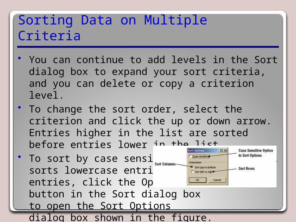
• You can continue to add levels in the Sort dialog box to expand your sort criteria, and you can delete or copy a criterion level.
• To change the sort order, select the criterion and click the up or down arrow. Entries higher in the list are sorted before entries lower in the list.
• To sort by case sensitivity, so that Excel sorts lowercase entries before uppercase entries, click the Options button in the Sort dialog boxto open the Sort Options dialog box shown in the figure.

Step-by-Step: Sort Data on Multiple Criteria
• USE the workbook from the previous exercise. 1. Select the range A2:E27, if it isn’t already
selected.2. Click Sort in the Sort and Filter group on the
Data tab to open the dialog box.3. Select Job Title in the Column section’s Sort By
box and A to Z in the Order box.4. Click the Add Level button in the dialog box to
identify the second sort criteria. A new criterion line is added to the dialog box.

Step-by-Step: Sort Data on Multiple Criteria
5. In the Then By box in the Column section select Last Name as the second criterion. A to Z should be the default in the Order box as shown in the figure. Click OK. You have now sorted using multiple criteria; first byjob title and then alphabeticallyby last name.
6. SAVE the workbook. • LEAVE the workbook open to use in the next
exercise.

Sorting Data Using Conditional Formatting
• If you have conditionally formatted a range of cells with an icon set, you can sort by the icon. Recall that an icon set can be used to annotate and classify data into categories.
• Each icon represents a range of values. For example, in a three-color arrow set, the green up arrow represents the highest values, the yellow sideways arrow represents the middle values, and the red down arrow represents the lower values.
Sorting Data Using Conditional Formatting
• The first time you perform a sort, you must select the entire range of cells, including the column header row.
• When you want to sort the data using different criteria, select any cell within the data range and the entire range will be selected for the sort.
• You need to select the data only if you want to use a different range for a sort.

Step-by-Step: Sort Using Conditional Formatting
• USE the workbook from the previous exercise. 1. On the Home tab, click Find & Select in the
Editing command group, and click Conditional Formatting in the drop-down menu. A message is returned that no cells in the worksheet contain conditional formatting. Click OK to close the message box. This step is to make sure there are no conditional formatting rules in place.

Step-by-Step: Sort Using Conditional Formatting
2. Select D3:D27. Click Conditional Formatting in the Styles group, and then open the Icon Sets gallery. See the figure below.

Step-by-Step: Sort Using Conditional Formatting
3. Click the 3 Arrows icon set. Each value in the selected column now has an arrow that represents whether the value falls within the high, middle, or low range of your data.
4. Select A3:E27. On the Home tab, click Sort & Filter and then click Custom Sort (see the figure); the Sort dialog box opens.
Step-by-Step: Sort Using Conditional Formatting
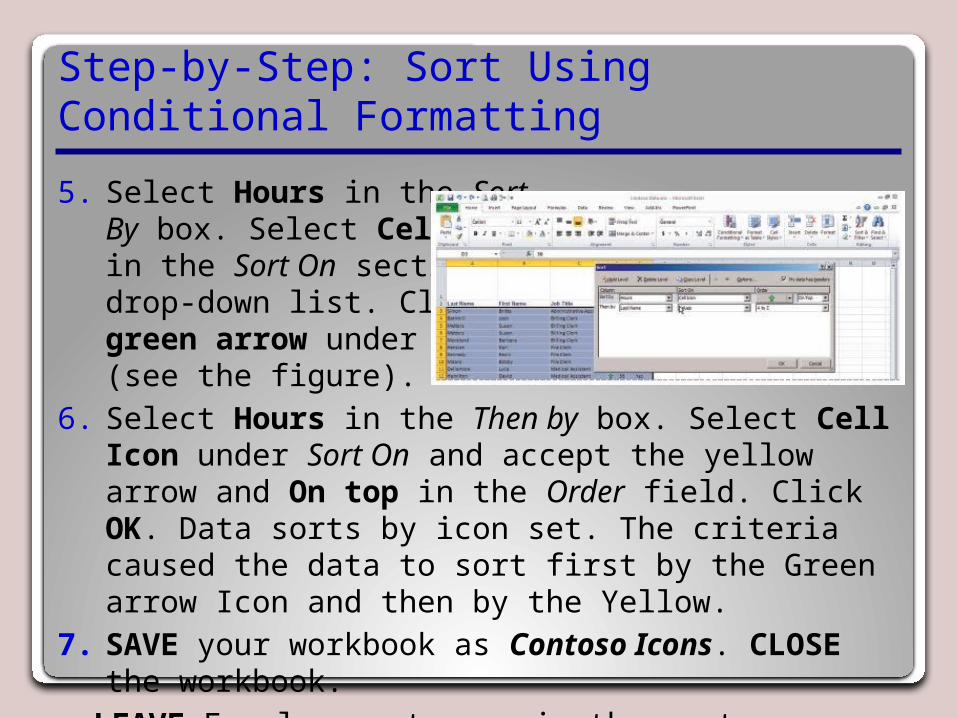
5. Select Hours in the Sort By box. Select Cell Icon in the Sort On section’s drop-down list. Click the green arrow under Order (see the figure).
6. Select Hours in the Then by box. Select Cell Icon under Sort On and accept the yellow arrow and On top in the Order field. Click OK. Data sorts by icon set. The criteria caused the data to sort first by the Green arrow Icon and then by the Yellow.
7. SAVE your workbook as Contoso Icons. CLOSE the workbook.
• LEAVE Excel open to use in the next exercise.

Sorting Data Using Cell Attributes
• If you have formatted a range of cells by cell color or by font color, you can create a custom sort to sort by colors.
• In the next exercise, you learn to sort by cell attribute (in this case, color) using the Sort dialog box to select the order in which you want the colors sorted.
• At Contoso, Ltd., each medical assistant is assigned to work with a specific physician. To assist with scheduling, the office manager created the MA Assignments worksheet with color-coded assignments for the physician/medical assistant. The color coding serves as a reminder that the two must be scheduled for the same days and hours when the weekly schedule is created. Color coding enables you to sort the data so that the work assignments are grouped for the physician and his or her medical assistant.

Sorting Data Using Cell Attributes
• Most sort operations are by columns, but you can custom sort by rows. Create a custom sort by clicking Options on the Sort dialog box. You can then choose Sort left to right under Orientation.
• Sort criteria are saved with the workbook so that you can reapply the sort each time the workbook is opened. The following table summarizes Excel’sdefault ascending sort orders. The order is reversed for a descending sort.

Step-by-Step: Sort Data Using Cell Attributes
• OPEN the MA Assignments data file for this lesson.
1. Select the entire data range (including the column headings). On the Data tab, click Sort.
2. In the Sort dialog box, accept Last Name in the Sort By box. Under Sort On, select Cell Color.
3. Under Order, select Pink and On Top.4. Click the Add Level button in the dialog box and
select Last Name in the Sort By box. In the Sort On section, select Cell Color. Select Yellow and On Top in the Order section.

Step-by-Step: Sort Data Using Cell Attributes
5. Using the same method you used in step 4, add a level for Green and then add a level for Blue. You should have a criterion for each color as illustrated in the figure. Click OK.
6. SAVE the workbook in your Lesson 7 folder as MA Assignments.
• LEAVE the workbook open to use in the next exercise.

Filtering Data
• Worksheets can hold as much data as you need, but you may not want to work with all of the data at the same time.
• You can temporarily isolate specific data in a worksheet by placing a restriction, called a filter, on the worksheet. Filtering data enables you to focus on the data pertinent to a particular analysis by displaying only the rows that meet specified criteria and hiding rows you do not want to see.
• You can use Excel’s AutoFilter feature to filter data, and you can filter data using conditional formatting or cell attributes.

Using AutoFilter
• AutoFilter is a built-in set of filtering capabilities. • Using AutoFilter to isolate data is a quick and
easy way to find and work with a subset of data in a specified range of cells or table columns.
• You can use AutoFilter to create three types of filters: list value, format, or criteria. Each filter type is mutually exclusive. For example, you can filter by list value or format, but not both.
• In the next exercise, you will use AutoFilter to organize your data.

Using AutoFilter
• In the next exercise, you use two text filters to display only the receptionists and accounts receivables clerks.
• This information is especially useful when the office manager is creating a work schedule.
• This feature allows him or her to isolate relevant data quickly.

Step-by-Step: Use AutoFilter
• USE the workbook from the previous exercise. 1. Select A3:E28. Click
Filter on the Data tab in the Sort & Filter group; a filter arrow is added to each column heading.
2. Click the filter arrow in the Job Title column. The AutoFilter menu shown in the figure is displayed.

Step-by-Step: Use AutoFilter
3. Currently the data is not filtered, so all job titles are selected. Click Select All to deselect all titles.
4. Click Accounts Receivable Clerk and Receptionist. Click OK. Data for six employees who hold these titles is displayed. All other employees are filtered out. See the figure.
• LEAVE the workbook open with the filtered data displayed to use in the next exercise.

Creating a Custom AutoFilter
• You can create a custom AutoFilter to further filter data by two comparison operators.
• A comparison operator is a sign, such as greater than or less than, that is used in criteria to compare two values. For example, you might create a filter to identify values greater than 50 but less than 100. Such a filter would display values from 51 to 99.

Creating a Custom AutoFilter
• Comparison operators are used to create a formula that Excel uses to filter numeric data. The operators are identified in the following table.
• Equal to and Less than are options for creating custom text filters. Text Filter options also allow you to filter text that begins with a specific letter (Begins With option) or text that has a specific letter anywhere in the text (Contains option).

Creating a Custom AutoFilter
• As illustrated in the figure, you candesign a two-criterion custom filterthat selects data that contains both criteria (And option) or selectsdata that contains one or the otherof the criteria (Or option). If you select Or, less data will be filtered out, giving a much wider filter. When choosing the And option, it narrows your filtered data.
• Creating a filter is also known as “defining” a filter.

Step-by-Step: Create a Custom AutoFilter
• USE the workbook from the previous exercise.1. With the filtered list displayed, click the filter
arrow in column D. In the AutoFilter menu, point to Number Filters. As shown in the figure,the menu expands toallow you to customizethe filter.

Step-by-Step: Create a Custom AutoFilter
2. Select Less Than on the expanded menu and key 30 in the amount box. Click OK. The AutoFilter menu closes and the filtered list reduces to four employees who work fewer than 30 hours per week.
3. Click the Filter button in the Sort & Filter group on the Data tab to display all data. With the data range still selected, click Filter again.
4. Click the filter arrow in column D to open the AutoFilter menu. Point to Number Filters and select Greater Than. Key 15 and press Tab twice to move to the second comparison operator criteria box.

Step-by-Step: Create a Custom AutoFilter
5. Click the arrow for the comparison operator drop-down list and select is less than as the second comparison operator and press Tab. Key 30 and click OK. The list should be filtered to six employees.
6. Click the Filter button to once again display all data.
7. SAVE and CLOSE the workbook.• LEAVE Excel open to use in the next exercise.

Filtering Data Using Conditional Formatting
• If you have conditionally formatted a range of cells, you can filter the data by that format. A conditional format is a visual guide that helps you quickly understand variation in a worksheet’s data.
• By using conditional formatting as a filter, you can easily organize and highlight cells or ranges in order to emphasize the values based on one or more criteria.
• In the next exercise, you learn to use icon sets to identify the number of hours employees work each week.

Step-by-Step: Filter Using Conditional Formatting
• OPEN Conditional Format from the data files for this lesson.
1. Select A3:E32. On the Data tab, click Filter.2. Click the filter arrow in column D. Point to Filter
by Color in the AutoFilter menu that appears. Click the green flag under the Filter by Cell icon. Data formatted with a green flag (highest number of work hours) is displayed.
3. Click the filter arrow in column D. Point to Filter by Color. Click the red flag under the Filter by Cell icon. The data formatted by a green flag is replaced in the worksheet by data formatted with a red flag (lowest number of work hours).
4. Click Filter to remove the filter arrows.• LEAVE the workbook open to use in the next
exercise.

Filtering Data Using Cell Attributes
• If you have formatted a range of cells with fill color or font color, you can filter on those attributes.
• It is not necessary to select the data range to filter using cell attributes. Excel will search for any cell that contains either background or font color.
• In the next exercise, icon sets are used to identify the number of hours employees work each week, and font color has been used to identify the medical assistant assigned to each physician.
• In the next exercise, you will use font attributes as your filter criteria.

Filtering Data Using Cell Attributes
• In the preceding and next exercises, you used Excel’s Sort and Filter features to organize data using a variety of criteria.
• Both Sort and Filter allow you to select and analyze specific data. The two functions have a great deal in common. In both instances, you can focus on data that meets specific criteria.
• Unrelated data is displayed when you sort; it is hidden when you use the filter command.

Step-by-Step: Filter Data Using Cell Attributes
• USE the workbook from the previous exercise. 1. Select any cell in the data range and click the
Filter button in the Sort & Filter group on the Data tab.
2. Click the arrow next to the Title header (Contoso, Ltd.) and point to Filter by Color. Click More Font Colors. A dialog box opens that displays the font colors used in the worksheet.
Step-by-Step: Filter Data Using Cell Attributes
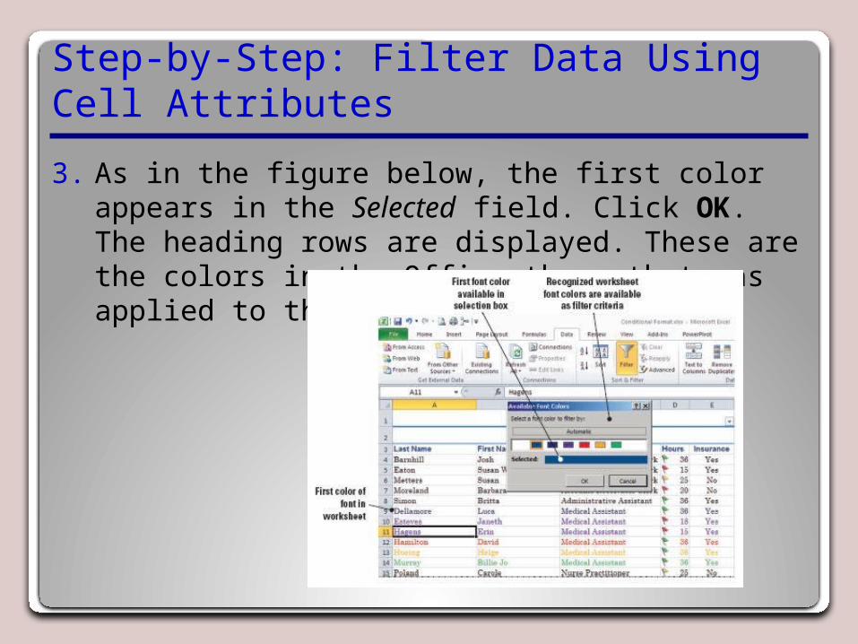
3. As in the figure below, the first color appears in the Selected field. Click OK. The heading rows are displayed. These are the colors in the Office theme that was applied to this worksheet.

Step-by-Step: Filter Data Using Cell Attributes
4. Click the filter arrow next to the Title header again and click Clear Filter From “Contoso, Ltd.”
5. Click the Title header filter arrow again and point to Filter by Color. Select Purple in the Filter by Font Color drop-down menu (3rd selection). Data for Dr. Blythe (new physician) and his two medical assistants is displayed because you chose the Purple font in your sort criteria.
6. Click the Filter button to clear the filter arrows.7. CLOSE the file. You have not made changes to
the data, so it is not necessary to save the file.• LEAVE Excel open to use in the next exercise.

Subtotaling Data
• Excel provides a number of features that enable you to organize large groups of data into more manageable groups.
• Data in a list can be summarized by inserting a subtotal.
• Before you can subtotal, however, you must first sort the list by the field on which you want the list subtotaled.

Grouping and Ungrouping Data for Subtotaling
• If you have a list of data that you want to group and summarize, you can create an outline.
• Grouping refers to organizing data so that it can be viewed as a collapsible and expandable outline.
• To group data, each column must have a label in the first row and the column must contain similar facts. The data must be sorted by the column or columns for that group.

Grouping and Ungrouping Data for Subtotaling
• In the preceding and next exercises, you manually grouped and subtotaled salary data for Contoso, Ltd. You will use Excel’s automatic subtotal feature in the an exercise later in this lesson.
• To outline data by rows, you must have summary rows that contain formulas that reference cells in each of the detail rows for that group.
• In the next exercise, your outline contained three levels: the grand total level, the subtotals level, and the detail rows level. You can create an outline of up to eight levels.
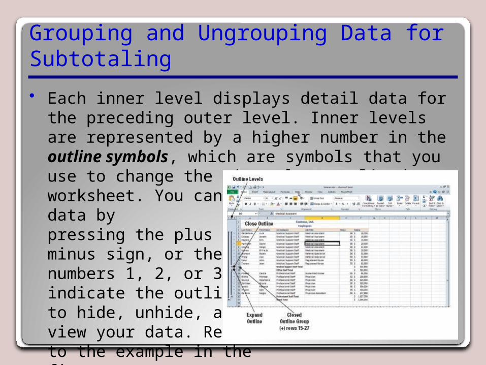
Grouping and Ungrouping Data for Subtotaling
• Each inner level displays detail data for the preceding outer level. Inner levels are represented by a higher number in the outline symbols, which are symbols that you use to change the view of an outlined worksheet. You can show or hide detailed data by pressing the plus sign, minus sign, or the numbers 1, 2, or 3 that indicate the outline level to hide, unhide, and view your data. Refer to the example in the figure.

Step-by-Step: Group and Ungroup for Subtotaling
• OPEN the Salary data file for this lesson.1. Select any cell in the data range. Click Sort on
the Data tab.2. In the Sort dialog box, sort first by Job Category
in ascending order.3. Add a sort level, sort by Job Title in ascending
order, and click OK.

Step-by-Step: Group and Ungroup for Subtotaling
4. Select row 14, press Ctrl, and select row 27. On the Home tab, click the Insert arrow in the Cells group and click Insert Sheet Rows from the drop-down menu that appears. This step inserts rows to separate the job categories. Refer to the figure.

Step-by-Step: Group and Ungroup for Subtotaling
5. In C14, key Subtotal. Select F14 and click the Sum icon (also shown in the figure on the previous slide). The values above F14 are selected. Press Enter and Excel subtotals the category.
6. In C28, key Subtotal. Select F28 and click Sum. Press Enter.
7. In C36, key Subtotal. Select F36 and click Sum. Press Enter.
8. In C37, key Grand Total. Select F37 and click Sum. The three subtotals are selected. Press Enter.

Step-by-Step: Group and Ungroup for Subtotaling
9. Select a cell in the data range. On the Data tab, click the Group arrow in the Outline group, and then click Auto Outline from the drop-down menu. A three-level outline is created. The figure shows your worksheet complete with subtotals and grand total. To view your worksheet as in the figure, adjust your zoom to 75%.
• LEAVE the workbook open to use in the next exercise.

Subtotaling Data in a List
• As you have learned, when data is not categorized, you can manually insert subtotals.
• When the data you want to subtotal can be grouped according to a category, the Subtotal command is the best choice.
• You can automatically calculate subtotals and grand totals for a column by using the Subtotal command in the Outline group on the Data tab.
• You can display more than one type of summary function for each column.

Subtotaling Data in a List
• The Subtotal command outlines the list so that you can display and hide the detail rows for each subtotal.
• In the next exercise, you will use the subtotal command to accomplish the various tasks.
• You can subtotal groups within categories, as well. For example, you could subtotal the salaries for the accounts receivable clerks or the records management employees as well as find a total for the entire office staff.
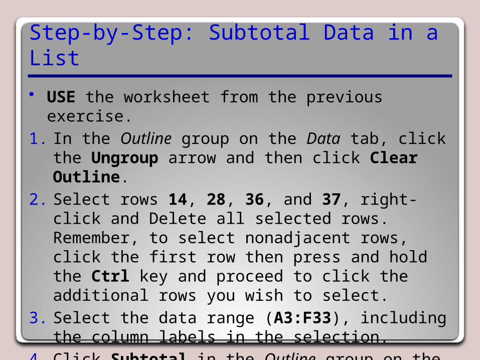
Step-by-Step: Subtotal Data in a List
• USE the worksheet from the previous exercise.1. In the Outline group on the Data tab, click the
Ungroup arrow and then click Clear Outline.2. Select rows 14, 28, 36, and 37, right-click and
Delete all selected rows. Remember, to select nonadjacent rows, click the first row then press and hold the Ctrl key and proceed to click the additional rows you wish to select.
3. Select the data range (A3:F33), including the column labels in the selection.
4. Click Subtotal in the Outline group on the Data tab. The Subtotal dialog box is displayed.
5. Select Job Category in the At Each Change in box.

Step-by-Step: Subtotal Data in a List
6. Under Add Subtotal To, Salary should already be checkmarked. Click OK to accept the remaining defaults. Subtotals are inserted for each of the three job categories, and a grand total is calculated at the bottom of the list. The figure has the outline groups with subtotals and grand total.
7. SAVE the workbook as Salaries.• CLOSE the workbook, but LEAVE Excel open for the
next exercise.

Setting Up Data in a Table Format
• When you create a table in Excel, you can manage and analyze data in the table independently of data outside the table.
• For example, you can filter table columns, add a row for totals, apply table formatting, and publish a table to a server.

Formatting a Table with a Quick Style
• You can turn a range of cells into an Excel table and manage and analyze a group of related data independently.
• When you create a table, a Design tab appears on the Ribbon offering Excel’s Table Tools. You can use the tools on the Design tab to customize or edit the table.
• By default, when you insert a table, the table has filtering enabled in the header row so that you can filter or sort your table quickly.

Formatting a Table with a Quick Style
• Four table styles are displayed in the Table Styles group. Click the arrows to the right of the styles to display additional styles. You can view the styles samples in the figure.
• In the next exercise, you will learn how to use a quick style.
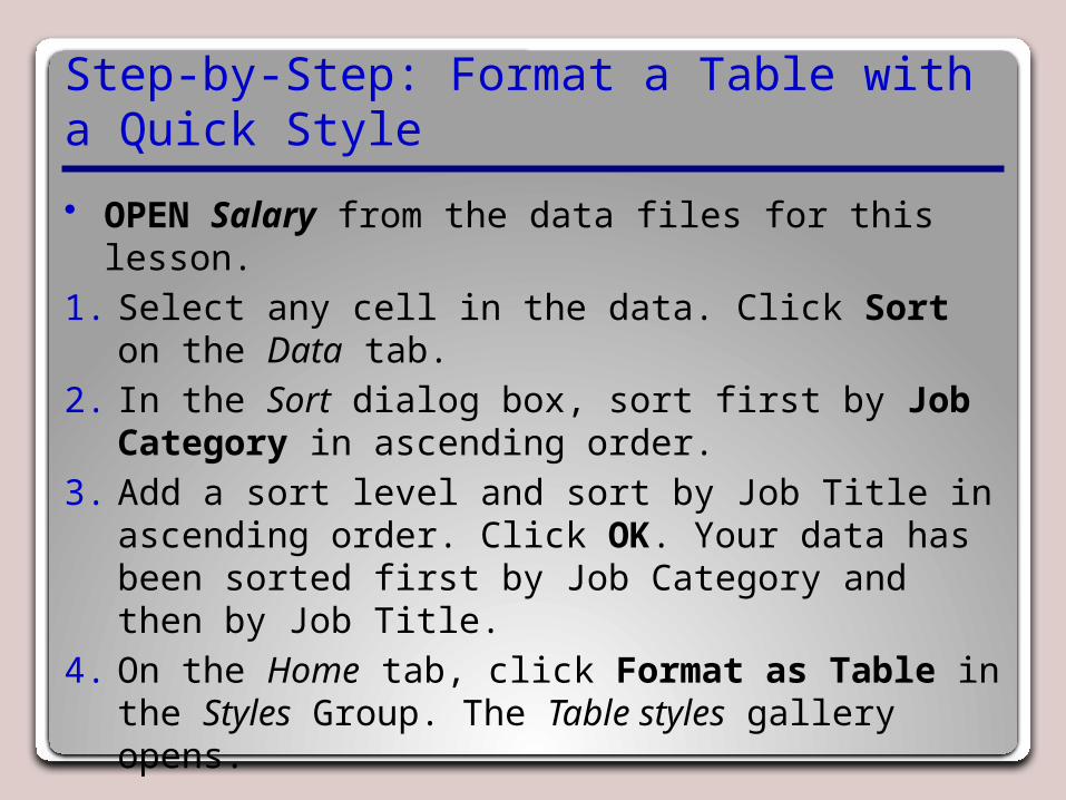
Step-by-Step: Format a Table with a Quick Style
• OPEN Salary from the data files for this lesson. 1. Select any cell in the data. Click Sort on the
Data tab.2. In the Sort dialog box, sort first by Job Category
in ascending order.3. Add a sort level and sort by Job Title in ascending
order. Click OK. Your data has been sorted first by Job Category and then by Job Title.
4. On the Home tab, click Format as Table in the Styles Group. The Table styles gallery opens.

Step-by-Step: Format a Table with a Quick Style
5. Mouse over the Table styles to Table Style Medium 5 from the gallery. The Format as Table dialog box opens.
6. Click the hide dialog box icon in the Where Is the Data for Your Table? box to collapse the Format as Table dialog box so you can select the data to be included in the table.

Step-by-Step: Format a Table with a Quick Style
7. Select A27:F32 as shown in the figure and press Enter. The Create Table dialog box appears. Your table does not have headers, so click OK. The Table Style Medium 5 format is applied and filtering column headers are inserted as illustrated in the figure on the next slide.

Step-by-Step: Format a Table with a Quick Style
8. SAVE the workbook as Table in the Lesson 7 folder.
• LEAVE the workbook open to use in the next exercise.

Using the Total Row Command in a Table
• To total your data, you could insert a new row at the end of the table. But it is faster to total the data in an Excel table by using the Total Row command in the Table Styles Options group on the Design tab.
• In the next exercise, you will use this command.• If you press Tab in the last cell of the last row of
the table, a blank row will be added at the end of the table, which would allow you to add new data to the table. Once a Totals row has been added to the table, however, pressing Tab will not add a new row.

Step-by-Step: Use the Total Row Command
• USE the workbook from the previous exercise.1. Select a cell inside the
table and click the Total Row command box in the Table Style Options group on the Design tab. A row is inserted below the table and the salaries in column F of the table are totaled. This is illustrated in the figure.
Step-by-Step: Use the Total Row Command
2. Click any blank cell to deselect the table. Adjust the column width to display the total amount if necessary. Click on any cell inside the table.
3. SAVE the workbook.• LEAVE the workbook open to use in the next
exercise.
Adding and Removing Rows or Columns
• After you create a table in your worksheet, you can easily add rows or columns.
• You can add adjacent rows to the table by using the mouse to drag the resize handle down to select rows or drag to the right to select columns.
• You can enter text or values in an adjacent row or column that you want to include in the table.
• You can add a blank row at the end of the table, or insert table rows or columns anywhere in the table.
• In the next exercise, you will learn to add and remove rows and columns.

Adding and Removing Rows or Columns
• When you resize a table, the table headers must remain in the same row, and the revised table range must overlap the original table range.
• In the exercise, you add a row from below to the table, but you are not able to add a row from above the table. You can click the resizing handle in the lower-right corner of the table and drag it to the right to add a column.
• When you finish working with a table, you can click Convert to Range in the Tools group and convert the table to a data range. The formatting, column headers, and table total remain.

Step-by-Step: Add and Remove Rows or Columns• USE the workbook from the previous exercise.1. On the Design tab, in the Properties group, click
Resize Table. The Resize Table dialog box opens.
2. Collapse the Resize Table dialog box by clicking the collapse dialog box button, and select A27:F35. Press Enter to accept the new range of cells. Click OK to accept the change to the table and apply the new settings. The physician assistant data is moved above the total line, and the total is recalculated. Refer to the figure.

Step-by-Step: Add and Remove Rows or Columns
3. Select C28. On the Home tab, click the Delete arrow in the Cells group, and click Delete Table Columns from the drop-down menu that appears. Column C is deleted. Refer to the figure for the drop-down menu.
4. Click the Column1 heading and key Last Name. Press Tab to move to the Column 2 heading. Key First Name in that column heading and press Tab to advance to the next heading. Key Job Title in the column 4 heading and press Tab.

Step-by-Step: Add and Remove Rows or Columns
5. Key Hours in column 5. Press Tab. In the Invalid Entry dialog box that displays, click Yes to continue. Clicking Yes here will override the data restrictions and dismiss the Invalid Entry dialog box. Key Salary in the column 6 heading and press Enter. Your table headings should appear as illustrated in the figure.

Step-by-Step: Add and Remove Rows or Columns
6. If necessary, adjust the column E width to display the total salary amount.
7. In the Properties group on the Design tab, select the text in the Table Name box and key Schedule and press Enter. This table represents the individuals with whom patients schedule appointments.
8. SAVE the file and then CLOSE the file.• CLOSE Excel.

Lesson Summary