5757 S. University Ave.

Chicago, IL 60637

Main: 773.702.5599

bfi.uchicago.edu

WORKING PAPER · NO. 2019-51

The Patent Troll: Benign Middleman or Stick-Up Artist? David S. Abrams, Ufuk Akcigit, Gokhan Oz, and Jeremy PearceMARCH 2019

The Patent Troll:Benign Middleman or Stick-Up Artist?∗

David S. Abrams Ufuk Akcigit Gokhan Oz Jeremy Pearce†

March 24, 2019

Abstract

How do non-practicing entities (“Patent Trolls”) impact innovation and technological progress?We employ unprecedented access to NPE-derived patent and financial data and a novel modelto answer this question. We find that NPEs tend to acquire litigation-prone patents from smallfirms and acquire patents less core to the seller’s business. When NPEs license patents, thosethat generate higher fees are closer to the licensee’s business and more litigation-prone. More-over, downstream innovation drops when patents are acquired by NPEs. Quantitatively, theoverall impact of NPEs depends on the share of infringements that come from non-innovatingproducers.

Keywords: Non-practicing entity, NPE, patent assertion entity, PAE, patent troll, innova-tion, patent litigation.

JEL Classification: O31, O34.

∗The authors would like to thank Alan C. Marco, Iain Cockburn, Ali Hortacsu, Casey Mulligan, Jill Grennan, MuratAlp Celik and seminar and conference participants at the U.S. Patent and Trademark Office, Stanford University, 5th

Annual Research Roundtable on Patents and Technology Standards, and University of Bordeaux for very helpfulfeedback and discussions. Akcigit gratefully acknowledges financial support from the Alfred P. Sloan Foundation, theEwing Marion Kauffman Foundation, and the National Science Foundation.†Author affiliations and contact information. Abrams: University of Pennsylvania Law School

& Wharton (dabrams@law.upenn.edu). Akcigit: University of Chicago Economics, NBER, & CEPR(uakcigit@uchicago.edu). Oz: Analysis Group (gokhan.oz@analysisgroup.com). Pearce: University of ChicagoEconomics (jgpearce@uchicago.edu).

1

“Having made a really meritorious invention, and having secured a patent thereupon, thebattle of the inventor, who would sell his patent, is just begun. Heretofore he may havedone some good skirmishing, but now he must face the music of solid battle."

William Edgar SimondsPractical Suggestions on the Sale of Patents, p.5, 1871

1 Introduction

Are Non-Practicing Entities (NPEs)1, often referred to as “Patent Trolls”, good or bad for tech-nological progress? This longstanding question has gained renewed urgency with their recentproliferation. Concern about potential negative effects of NPEs has led to the introduction oflegislation in state legislatures and Congress aimed at curtailing their activity. The view of theNPE as stick-up artist holds that they provide no benefits, but simply amass patents and holdup companies, using the threat of litigation to extract rents. At the same time, legislative effortshave been opposed by advocates who hold that NPEs can provide positive benefits akin to mar-ket intermediaries found in a range of industries. According to this view of the NPE as benignmiddleman, the market for patents requires intermediation to facilitate inventors monetizing theirideas and overcoming the frictions noted in the opening quote. Thus, inventors who are notwell-positioned to fully utilize their invention may sell or license them through an NPE’s largenetwork of industrial companies.

Despite the popularity and importance of the subject, the inner workings of NPEs have re-mained mysterious, and discussions about them have mostly been based on anecdotal evidence.This is largely because NPEs act in secrecy, making it harder for researchers to access micro dataon their direct business transactions and paid prices. We seek to inform this important debate byanalyzing extensive novel data obtained directly from large NPEs in order to understand theirimpact on innovation. We develop a new model that incorporates NPEs to frame our empiricalanalysis and calibrate it in order to understand whether NPEs facilitate or harm innovation.

This paper makes two major contributions to our understanding of NPEs. We first develop amodel of innovation based on quality-ladder growth models that incorporates NPEs and makestestable predictions. We then test the model by using a proprietary dataset with detailed financial,transaction and technological information on tens of thousands of NPE-held patents (Abramset al., 2018). We build on prior work that has developed important metrics for patents, such aslitigation risk (Lanjouw and Schankerman, 2001) and patent distance (Akcigit et al., 2016), whichquantifies the technological similarity between patents or groups of patents. While our datasetis quite large, it is far from the entire set of NPEs, and our empirical results should not be seenas universal or representative. They provide a new window into the impact of large professionalNPEs.

1We define an NPE broadly as a firm whose primary source of revenue is from patent licensing fees or patentlitigation awards. In Section 2 we discuss the relationship with related terms such as patent assertion entities (PAEs)or patent trolls.

Even though NPEs have received increased attention in recent years, middlemen in the marketfor ideas not a new phenomenon. In fact, the market for patents has been aided by intermediariesfor about as long as patents have existed. This market, like most, suffers from informationaland financial frictions that makes it harder to match the right buyers and sellers (Lamoreauxand Sokoloff, 1999). Intermediaries have the potential to serve an important function in thisregard (Khan, 2014). People with meritorious inventions look for channels whereby they can becompensated if they cannot make the best use of their invention. According to Lamoreaux andSokoloff (1999), 550 patent intermediaries were present in the 1880’s across the United States,working to build a bridge between buyers and sellers of patents. There were even extensiveguidebooks for interacting with patent intermediaries, such as Simonds (1871). Khan (2014,2015) also show how constant NPEs have been throughout history.

Our analysis begins with a theoretical investigation which we use to guide our empiricalanalysis. Following in the tradition of quality-ladder growth models (Aghion and Howitt, 1992;Grossman and Helpman, 1991), we build a new model of innovation where patents can be in-fringed and sold in the secondary market with the help of an intermediary. The intermediary hastwo potential roles: as benign middleman and stick-up artist. In the model, patents are producedwith multiple levels of uncertainty. First, as in classical models, the arrival rate of innovation isprobabilistic. Second, unlike the traditional models, a patent can have differential fit (i.e. patentdistance as in Akcigit et al. (2016)) to the original inventor. This creates an incentive for an inven-tor to sell a patent to another user if it does not fit the inventor’s portfolio well. An NPE, with itsmore extensive network of buyers and sellers, facilitates this transaction and serves as a benignmiddleman.

In the model, there is also some probability other firms will infringe a particular patent. Inthis case, the patent-holders can sue and win the case with a probability determined by theirlegal and financial resources, which we capture by firm size. In their second role as stick-upartist, NPEs can buy patents from weak inventors and use their legal power and new status asthe rightful owner of the patent to sue the infringing firm. This provides an incentive for smallerfirms to sell their patents to an NPE. We use this framework to generate a number of predictionswhich we then test with our data as we detail below.

In addition to deal-level acquisition and licensing data received directly from NPEs, we alsoconstruct an index for how likely a patent is to be litigated (following Lanjouw and Schankerman(2001)), and compute a distance measure that denotes how well a patent fits to a firm’s portfolio(following Akcigit et al. (2016)). These core measures allow us to examine several questions,which test predictions of the model: How do patent attributes, such as distance and likelihoodof litigation, impact the price paid by NPEs in acquisition deals? How does the entity size ofthe original assignee affect likelihood of sale and price? When NPEs license patents, what patentcharacteristics impact licensing revenue? Finally, using patent citation data, we also investigatehow the citation rate to patents varies around the time of acquisition by NPEs and whether thereis heterogeneity by patent value.

3

In our empirical investigation, we find that patent distance contributes positively to the like-lihood of a patent sale to an NPE, especially for large firms. Examining the source of NPE-heldpatents, we also find that they buy patents predominantly from smaller entities, and more so forlitigation-prone patents. With another novel feature of our data, acquisition prices, we find thatNPEs pay more for patents from large firms. We also find that NPEs pay less for patents that area worse fit (greater distance) for the original inventor. Next, we focus on licensing transactionsand find that NPEs receive higher fees from patents that have a lower distance (better fit) to thelicensee’s portfolio. All of these findings corroborate predictions made in the model. Finally,we find a decline in citations to NPE-acquired patents upon acquisition. This decline is drivenprimarily by high-value patents.

Our theoretical and empirical analysis is agnostic about the overall impact of NPEs on newtechnology creation since the existence of NPEs can have both positive and negative effects oninnovation incentives. In order to understand the net effect of NPEs, we undertake a numericalexercise in which we bring the model closer to the data by matching a number of informativemoments in our data using Simulated Method of Moments (SMM). We find mixed results de-pending on the quantitative magnitudes of the role of the benign middleman and stick-up artistmechanisms. The ultimate effect of NPEs on innovation depends on the source of patent in-fringement. If the majority of infringement comes from innovating producers, we find that thestick-up artist role dominates and NPEs reduce the overall innovation effort in the economy. If asignificant majority of infringement is due to non-innovating producers, the benign middlemanrole dominates and NPEs increase the overall innovation effort.

Taken together, the evidence in this paper does not solely support the benign middlemanor the stick-up artist theory. Rather, it suggests that there are some aspects of NPEs that mayincrease aggregate innovation and some that may not. As debate continues both in academiaand the policy world, it will be helpful to keep these benefits and costs in mind. The rest ofthe paper is organized as follows. Section 2 provides some institutional details and a summaryof the literature. In Section 3 we present our model of innovation with NPEs, stressing themultiple roles NPEs can play. In Section 4 we introduce the data with the main empirical resultspresented in Section 5. Section 6 presents the numerical analysis and calibration exercise. Section7 concludes.

2 Background and Related Literature

Since the terms patent troll, NPE, and patent assertion entity (PAE) are frequently used to denotesimilar or overlapping entities, it is useful to have a clear definition of what we study in thispaper. We define an NPE broadly as a firm whose primary source of revenue is from patentlicensing fees or patent litigation awards. This can include a large array of entities, from in-dividual inventors who do not practice their inventions, to shell companies that file hundredsof lawsuits, to universities, to patent aggregators whose primary revenues come from licensing

4

fees. Some use the term PAE almost synonymously to NPE, but excluding entities that performresearch, such as universities (and potential inventors who still invent). We here also excludea related group of legal entities that issued demand letters to hundreds of businesses allegingpatent infringement for the use of networked scanners to email documents.2

We will use the term NPE in this paper and focus on large firms that purchase patents andprimarily license them or litigate when they cannot license. We focus on this category for severalreasons. First, these are the types of NPEs receiving the most attention from the media andlegislatures in recent years. They are also arguably the most interesting case because there areplausible positive and negative attributes. In addition, university licensing is unlikely to becomea hot policy issue. Finally, not only is their effect on innovation more contentious and uncertain,these large firms are most likely making the biggest impact of the set of middlemen in marketsfor innovation.

Related Literature This paper contributes to an extensive literature that links the role of patentsto growth in the aggregate economy. In particular, Eaton and Kortum (1996) estimate a modelto explain international patterns of productivity and patenting while Jaffe and Trajtenberg (1999)show how international knowledge flows occur through patents. Akcigit et al. (2017) show thateconomies that produce more patents also grow faster in the long-run. Kortum (1997) emphasizesthe role of searching for ideas in linking patents to productivity growth. As Ahmadpoor andJones (2017) and Henderson et al. (1998) show, patents can contribute to aggregate productivitythrough channeling basic academic research to products. Caballero and Jaffe (1993) estimate aquality-ladder model using patent data to quantify the role of creative destruction on economicgrowth. At a more micro level, Bloom and Van Reenen (2002) show that patents have a significantimpact on firm-level productivity and market value. Blundell et al. (1999) find a strong and robusteffect of the headcounts of innovations and patents on market share.

In the theoretical model, we build on endogenous growth theory where ideas are the fun-damental building blocks of long-run growth. Our framework applies quality ladder modelsfollowing in the tradition of Aghion and Howitt (1992), Grossman and Helpman (1991), Kletteand Kortum (2004), Lentz and Mortensen (2008), Acemoglu et al. (2018) and Akcigit and Kerr(2018). Other papers in this space, i.e. Benhabib et al. (2014), Konig et al. (2016), and Perla andTonetti (2014) focus on how growth emerges initially from innovation but also from imitation astechnologies ripple through the economy. Patents here can serve as a channel for incentivizingidea creation, making information available to the public, as well as increasing the value of afirm.

For the most part, idea transfer and middlemen in the market for ideas has not been centralto the theory of growth–but as Serrano (2010) and Akcigit et al. (2016) note, the transfer of ideascan be key for a firm building its portfolio. Within the quality ladder framework, Akcigit et al.(2016) address the misallocation and reallocation of ideas being a key contributor to economic

2See http://arstechnica.com/tech-policy/2013/01/patent-trolls-want-1000-for-using-scanners/

5

growth. In another theoretical exploration, Chatterjee and Rossi-Hansberg (2012) discuss howidea “spinoffs” can be fundamental to growth and address problems of information asymmetryin marketing new ideas. Although the role of NPEs is not addressed in this literature, theseinvestigations leave a large space for a middleman that can reduce informational frictions.

Serrano (2010, 2018) finds that patent renewal and transfer is an important component ofinnovation. As such, there seems to be a role for the NPE in serving as a important player inthis market. Indeed, Akcigit et al. (2016) find that the secondary market in patents is mostlygoverned by middlemen. Griffith et al. (2003, 2004) find that R&D investment also allows firmsto generate “absorptive capacity,” as firms may spend more on R&D with the expectation thatthey can engage in technology transfer through middlemen. This absorptive capacity may alsomake firms more likely to be linked to networks of patent middlemen–with capabilities to moveon ideas the firm itself does not create.

This paper also contributes to a rich literature on industrial policy, knowledge spillovers(Bloom et al., 2013), and firm size e.g. (Garicano et al., 2016). In particular, we focus on issuesrelated to patent and innovation policy. Galasso and Schankerman (2015) use exogenous vari-ation from patent examination and invalidation and find a heterogeneous effect of changes inpatent rights on downstream innovation, significantly depending on industry. We may expectthe NPE to reflect this underlying reality, as areas with high litigation may induce the NPE tofulfill their role through their legal resources. In areas where downstream innovation is unaf-fected, the NPE may indeed be a benign middleman simply serving the role of improving ideaallocation. Galasso et al. (2013) use exogenous changes in tax rates and find that taxes stronglyaffect the market for innovation. In addition, they find the reallocation of patent rights reduceslitigation risk, indicating that patents are moving to more highly valued owners.

We unite this mostly theoretical growth literature with a burgeoning empirical literature onthe role of NPEs in the market for innovation that has primarily focused on the role of NPE asstick-up artist. The biggest challenge of this set of papers has been data limitations. As discussedearlier, NPEs often operate in private and it is very hard to get at both the transactions and theunderlying prices of these transactions. However, some creative papers have tried to measurethis NPE impact through various methods.

Some studies attempt to measure the impact of NPE assertions outside of the courtroom,drawing from data beyond claims litigated to finality. In a well-known study, Bessen and Meurer(2014) utilized survey data gathered by RPX, a risk-management company helping firms dealwith patent litigation. RPX invited 250 (nonrandomly selected) firms to participate in the survey,of which 82 provided information on lawsuits, and 46 provided information on non-litigation as-sertions (such as demand letters). Bessen and Meurer (2014) concluded from this limited samplethat NPE assertions resulted in $29 billion in direct costs, disproportionately burdening smallerand medium-sized companies. Similarly, Chien (2014) relied on nonrandom survey responsesand a database of patent cases, curated by RPX, to conclude that most defendants in NPE suitsare smaller companies. Through polling in-house attorneys across an array of industries, Feld-

6

man and Lemley (2015) find that when an NPE expressed an interest in licensing from firms,it did not induce further innovation. Lu (2012) finds the royalty rates paid to NPEs are similarto those paid to practicing entities, using information from vendors that aggregate royalty ratesprimarily drawn from companies’ public SEC filings.

Tucker (2014) focuses on the heathcare technology industry and finds a large reduction insales of defendants’ software projects that were allegedly infringed by a selected NPE’s patents,while surrounding products and firms did not see the same effect. A limitation of this study isthe single focus on defendants. When Kiebzak et al. (2016) look across industry by district pairs,they find that venture capital investment and patent litigation follows an inverted-U relationship.This could indicate how litigation to protect patents both holds back investment and induces newinnovators.

Another strain of research focuses solely on litigated cases, deriving information on NPEactivity from awarded damages or whether an asserted patent is found invalid. Risch (2012)attempted to defend the decision to only include litigation data in a study of the 10 most litigiousNPEs by asserting that it is more likely that litigious NPEs’ activities incur greater social costs.Cohen et al. (2016, 2017, 2018) used proprietary data from PatentFreedom, another companythat aggregates litigation data, in arguing that NPEs are more likely to target cash-rich firms.However, Ashtor et al. (2013) rejected the notion NPE litigation activity differs significantly frompracticing entity patent assertions. They examined over 1,750 patent cases litigated to a verdict,and found little difference in outcomes between NPEs and practicing entities. Cotropia et al.(2014) hand-coded information about the litigants in all patent infringement lawsuits filed in 2010and 2012, concluding that the hype about the dangers posed by NPE litigation is overblown.

Some scholars, including Schwartz and Kesan (2014), have questioned the generality of con-clusions based on data that is potentially unrepresentative and unreliable. They suggest thatthere may be an overemphasis on technology firms, and express concerns about varying def-initions of what constitutes an NPE. In terms of using litigation data, the aggregate economiceffect of NPEs may be underestimated, since many assertions may take place outside the scopeof publicly accessible records. Instead, NPEs may rely on extracting licensing royalties, much ofwhich is contractual and not subject to public disclosure.

Fischer and Henkel (2012) may not be subject to this problem as the classify NPEs usingpublic searches, newspapers, blogs, and websites. With these identified NPEs, they then searchthe patent assignment databases to arrive at a sample of patent acquisitions by NPEs. Usingproxy indicators for various characteristics of the acquired patents, they conclude that NPE-acquired patents are likely to be higher-quality and of broader scope and application than non-NPE patents.

Czarnitzki and Toole (2011) explore the role of patent protection in mitigating uncertainty,something which a reliable intermediary can improve. Toole and Turvey (2009) find that reduc-ing risk, in turn, can lead to increases in follow-on funding. This would be especially valuablefor liquidity-constrained small firms–the types of firms we find most commonly selling to NPEs.

7

This complements Haber and Werfel (2015, 2016) who present experimental evidence that NPEsprovide insurance and liquidity to firms by committing resources to protecting inventors’ prop-erty rights.

Lemley and Feldman (2016) argue that NPEs are more prominent in litigation than in fa-cilitating intellectual property transfers. They discuss the expanding importance of NPEs inthe market for patents, indicating that NPEs account for the majority of patent lawsuits filed.However, Cotropia et al. (2014) note that when we focus on the number of alleged infringers asopposed to cases, as in Lemley and Feldman (2016), there is little increase in NPE share of liti-gation. While Lemley and Feldman (2016) suggest the idea of the middleman is not convincing,they caution that the evidence is from small sample survey data.

When it comes to NPEs, the underlying legal institutions will be a relevant concern. Fengand Jaravel (2017) find that heterogeneity in patent outcomes is often based on how the rightsare crafted in the examination process. They find that NPEs are active in targeting patents with“lenient” examiners–backing up the story that NPEs can act as stick-up artists. As Marco andMiller (2017) and Graham et al. (2015) note, problems in the examination process can lead topatents having a higher risk of litigation. There are cases where patent thickets and aggregation,in particular from NPEs, can reduce innovation. If this is prominent, we can see how problems inthe underlying property institution can induce NPEs to act more as stick-up artist than middle-man, which could be linked to the “destructive” role of patents, which Nicholas (2013) addressesin general. Our paper allows for both channels discussed in this section. We start with the modelto frame our empirical analysis.

3 Model

In this section, we build a tractable model of production with innovation to address the roleNPEs play in the market for innovation. By examining a firm’s decision to sell to an NPE orlicense from one, our goal is to find theoretical implications for the stick-up artist and benignmiddleman views of NPEs, which we then test with data. The model generates a number ofpredictions about how patent and firm characteristics, such as patent fit (distance), litigation risk,and firm size, impact the decision to sell or license; in addition, the model generates predictionson how these characteristics affect the prices at which NPEs buy and license. This providesthe framework that will guide our empirical analysis in Section 5 and inform our calibration inSection 6.

Basic Environment Consider a simple economy represented by a unit circle C, as in Figure 1a.There are many intermediate-good-producing firms that are located along that unit circle, eachof which produces a differentiated good i. A unique final good is produced from a combinationof all these intermediate goods as follows: Y = 1

1−σ

∫C qσ

i k1−σi di, where ki denotes the quantity

and qi the quality of intermediate good i used in final good production. The final-good sector

8

Figure 1: Model Economy, Unit Circle C

r = 1/π

Firm k

Firm i

(a) Example of Two Firms i and k

r = 1/π

dkdi

Firm k

Firm i

Patent z(b) Two Firms and a Patent z

operates with perfect competition, and we normalize the price of the final good to 1 without anyloss of generality. Therefore, the objective function in the final-good sector is simply:

maxki

1

1− σ

∫C

qσi k1−σ

i di−∫C

Pikidi

, ∀i ∈ C.

where Pi is the price of variety i. This maximization problem delivers the following demandfunction for each intermediate good i:

Pi = qσi k−σ

i . (1)

Each intermediate good i is produced by a monopolist who owns a patent for their cuttingedge technology. The monopolist can produce ki at a constant marginal cost ψ in terms of theunique final good. Each monopolist firm chooses a price and quantity to maximize profits onits product line, taking the demand in (1) into account. The profit-maximization problem of themonopolist with a cutting edge technology for intermediate good i can then be written as

Πi = maxki≥0

qσ

i k1−σi − ψki

.

The first-order condition of this maximization problem implies a constant markup over marginal

cost, Pi = ψ/(1− σ), and thus ki =[(1−σ)

ψ

] 1σ qi. Equilibrium profit for a product line with tech-

nology qi isΠi = πqi, (2)

where we define π ≡ σ [(1− σ) /ψ]1−σ

σ .

The usual firm size proxies, such as profits Πi = πqi, and sales Piki = [(1− σ) /ψ]1−σ

σ qi, bothincrease linearly in quality qi. Therefore, in what follows, we proxy for firm size using qi.

9

3.1 Patents

Patent Distance and Firm Quality The circumference of the circle C in Figure 1 is normalizedto 2 such that the maximum distance between any two points along the circle is equal to 1. Likefirms, innovations (patents) in production are located along the circle. Figure 1b illustrates thisin an example. Firms i and k are located in different parts of the circle. There is a patent z thathas a distance di to firm i and dk to firm k.

Firm quality improves upon the invention or acquisition of new, patented innovations. Con-sider an innovating firm i. Its quality improves according to the following law of motion

qnewi = qi + γxi

where γ is some scale parameter and xi ∈ [0, 1] is the goodness of fit of the patent to the firm,which is the inverse of patent distance di ∈ [0, 1]:

di = 1− xi.

Low values of di (i.e., high xi) indicate that a patent is a good fit to the firm i. Given thelinearity of the profit function in (2), the incremental gain to monopolist i from using this patentis

∆Πi = π [qi + γ (1− di)]− πqi

= πγ (1− di) .(3)

Given that π and γ will appear multiplicatively for the rest of the analysis, we normalize γ = 1such that

∆Πi = π (1− di) . (4)

3.2 Non-practicing Entities

There are NPEs in this economy that may act as (i) middlemen or as (ii) stick-up artists. They havetwo key features: First, they have a broad network of firms to which they may license patentsas middlemen. Second, they have substantial financial and legal resources, which increase theirlikelihood of winning a case in court when they act as a stick-up artist. We detail these featuresnow.

The Middleman Any firm i that owns a patent can decide to keep its patent or sell it to theNPE. The NPE, through its wide network in the market, can potentially find a user k that is abetter fit for the patent with shorter distance dk < di or larger profit scale, Ωk (discussed below).Having access to a large network is the first advantage of the NPE over a single innovating firm.To keep things tractable and allow for focus on other dimensions, we use this as a reduced form

10

treatment, which is microfounded in Akcigit et al. (2016).

The Stick-up Artist The second key ingredient of our model is that patents may be infringedupon by other firms. Let us denote the firm that infringes on firm i’s patent by j. When j infringeson i’s patent, firm i can go to court and sue j. Winning a court case depends on resources thata firm has to fight in the court, as has been empirically shown in Haber and Werfel (2015, 2016).We capture this by assuming that a firm i wins the lawsuit with probability βi where βi increasesin firm size such that:3

βi = β(qi) and β′(qi) > 0.

The second strength of the NPE is that it has greater experience and resources to fight incourt, i.e., it has a high probability of winning in court, βnpe. Therefore, when a firm does nothave enough resources and faces a risk of infringement, it might be desirable for the firm to sellthe patent to an NPE.

We describe the rest of the dynamics of the model with the help of the game tree shown inFigure 2.

Figure 2: Game Tree

Distance di ∈ [0, 1],cost of NPE contact

ε ∈ [0, κ] are realized

Firm i,Vkeep

i

Vcourti

i goes to court

pi,j

i and j settle

j infringes

withprobability

α

Vprodi

i producesNo infringementwith probability (1− α)

i keeps patent

NPE,Vnpe

Vcourtnpe

NPE goes to court

pnpe,j

NPE and j settle

j infringes

with probability α

pnpe,kLicense to some k

for production with dk

No infringementwith probability (1− α)

i sells to NPEfor pi,npe

3Our analysis relies on the fact that an NPE and a patent producer have differential bargaining and/or negotiatingpower on the market. To keep the math tractable, we will assume symmetric bargaining power throughout yetdifferential negotiating power across firms and NPEs. Alternatively, one can model the bargaining power (instead ofthe winning probability) as a function of the firm size. The results would go through the same way, yet the expressionswould be less tractable.

11

In the beginning of the game, firm i produces a patent with a random distance di ∈ [0, 1] withmean νi. In addition, firm i realizes an idiosyncratic cost of finding an NPE, ε. Next, it decideswhether to sell it to the NPE or keep it within the firm.

If it decides to keep the patent, then the game evolves according to the upper branch.4 Beforeproduction takes place, the patent is infringed with probability α. While α is assumed to beexogenous in this section, it will be endogenized in Section 6. If there is no infringement, whichhas probability (1− α) , then the firm produces and collects the end-of-period return Vprod

i whichis simply equal to the marginal profit (the additional profit that the firm makes by using its newpatent)

Vprodi = π (1− di) .

If there is infringement, which happens with probability α, then i can no longer procure theincremental profits without patent enforcement; thus i will try to settle with j. If they cannotsettle, i goes to court and wins with probability βi. When i wins the case, it gets compensated forlost profits π (1− di). Hence, the expected value of going to court is:

Vcourti = βiπ (1− di) . (5)

Let Ωj denote the profit that j is making by infringing i’s patent. When the court decides in favorof i, then firm j also loses Ωj. Settlement generates a surplus that the two parties split throughNash bargaining with equal bargaining power for both sides. Let us denote the settlement (li-censing) fee that i will collect from j by pi,j. Then the fee is simply the solution to the followingproblem

pi,j = arg max(

pi,j −Vcourti

)0.5 (Vcourti + βiΩj − pi,j

)0.5 . (6)

Note that player i could receive Vcourti if there is no agreement and therefore her net surplus

from bargaining is pi,j − Vcourti . Likewise, player j will need to pay Vcourt

i and also give up hisΩj additional profit if the case goes to court and the court decides in favor of i with probabilityβi. Therefore j’s surplus from bargaining is Vcourt

i + βiΩj. This problem delivers the followingsettlement amount

pi,j = Vcourti +

βiΩj

2,

where Vcourti is expressed in (5). The settlement fee that j pays i is increasing in i’s probability of

winning the case βi, and in the profit that firm j is making by infringing i’s patent.

Now, going back one step in the game tree in Figure 2, we can calculate the expected value

4Since our focus on this paper is the role of an NPE, we do not model the possibility of a patent owner selling herpatent to the end user. This structure is imposed without apology since patents are sold mainly through intermediariesdue to their larger networks, as described in Akcigit et al. (2016).

12

to i of keeping the patent as

Vkeepi = αpi,j + (1− α)Vprod

i

= αβi

[π (1− di) +

Ωj

2

]+ (1− α)π (1− di) .

(7)

Next, consider what happens if i decides to sell the patent to the NPE, as illustrated by thelower branch. With probability α, there is a chance that j infringes the patent that now belongsto the NPE. In this case, the NPE can go to court or settle with j.5 There are two differences from(6): one is that the NPE by definition does not produce and therefore does not have π (1− di) asa bargaining chip. However, the NPE can block j from gaining Ωj and has potentially a higherprobability of winning, βnpe. Therefore, the problem for the settlement can be written as

pnpe,j = arg max(

pnpe,j)0.5 (

βnpeΩj − pnpe,j)0.5

which delivers the following settlement fee that the NPE will charge j:

pnpe,j =βnpeΩj

2.

If there is no infringement with probability (1− α), the NPE licenses the patent to some firm kwith a distance equal to dk ∼ Dk, which is taken from a uniform distribution on the unit circle.and profit equal to Ωk. The price again is determined through Nash bargaining as follows:

pnpe,k = arg max[pnpe,k

]0.5 [Ωk (1− dk)− pnpe,k]0.5 .

The price is simply

pnpe,k =Ωk (1− dk)

2.

With these prices, we can compute the expected value to the NPE of owning the patent:

Vnpe = αpnpe,j + (1− α) pnpe,k. (8)

At this point, we have solved for the end-game values in each state of the world. Knowing thecontinuation values in each branch of Figure 2, how much would the inventor i charge the NPEfor a patent sale? We are now ready to solve for the bargaining problem between i and theNPE. After the realization of the distance, firm i can sell the patent to the NPE through Nashbargaining. If Vnpe > Vkeep

i , this problem can be written as

pi,npe = arg max(

pi,npe −Vkeepi

)0.5 (Vnpe − pi,npe

)0.5 . (9)

5Note how, in equilibrium, no party goes to court. Yet, the possibility of going to court generates a threat thataffects that bargaining through the outside option.

13

Hence, the equilibrium price that firm i charges the NPE is:

pi,npe =Vkeep

i + Vnpe

2, (10)

where Vkeepi is expressed in (7) and Vnpe in (25). We assume that there is a cost of contracting

with an NPE, ε, that comes from a uniform distribution as ε ∼ U[0, κ]. There will be a salebetween i and the NPE if and only if there is a potential surplus that is bigger than the cost,pi,npe −Vkeep

i > ε. Therefore, the probability of sale can be written as

Pr (sale) =pi,npe −Vkeep

iκ

(11)

3.3 Model Predictions

In this section, we generate a number of important comparative statistics that we later test usingmicro data.6 First, we focus on the determinants of the probability of a patent sale to the NPE in(11). Our first result relates to the NPE’s role as a stick-up artist, and describes how patent salerelates to litigation risk and firm size.

Prediction 1 The NPE is more likely to buy patents from small firms:

∂

∂qiPr (sale) = −β′(qi)α

2κ

[π (1− di) +

Ωj

2

]< 0.

Moreover, this effect is more pronounced for litigation-prone patents:

∂2

∂α∂qiPr (sale) = −β′(qi)

2κ

(Ωj

2+ π (1− di)

)< 0.

This follows from the fact that small firms have a harder time defending themselves in court (i.e.,small βi). As a result, the NPE purchases patents from small firms in order to enforce their patentrights in the case of infringement. Thus, the NPE purchases more often from smaller firms, andat even more so for litigation-prone patents.

Next, we focus on the NPE as a middleman, which reallocates innovations to reduce thedistance to the owning firm.

6We write out the math for the proofs more complete in Appendix D

14

Prediction 2 The likelihood of a patent sale increases as the distance of the patent from the initialinnovating firm increases:

∂

∂diPr (sale) =

αβiπ + (1− α)π

2κ

> 0.

Moreover, this effect is more pronounced for large firms, i.e.,

∂2

∂di∂qiPr (sale) =

β′(qi)απ

2κ

> 0.

The intuition for this result is that patents that are a poor fit with the inventing firm will notbe well-utilized. The inventing firm will therefore consider selling it in the secondary marketthrough the NPE. This is especially true for large firms. Because large firms have greater courtcapability, they are more likely to use the NPE to reduce distance. Thus, the impact of distanceon probability of sale is more pronounced for large firms.

Our model has clear predictions on the sale price of a patent that was expressed in (10). Wenow turn to these predictions.

Prediction 3 The NPE pays more for large firms’ patents:

∂pi,npe

∂qi=

β′(qi)α[π (1− di) +

Ωj2

]2

> 0.

The equilibrium price of a patent is determined through Nash bargaining as described in (9).Since legal strength and resources are increasing in firm size, the outside option of a patent ishigher for large firms. Hence, large firms receive a higher price for their patents.

Next, we focus on the link between sale price and patent distance.

Prediction 4 The acquisition price decreases as patent distance to the seller increases:

∂pi,npe

∂di= − [αβi + 1− α]π

2

< 0

The intuition for this result is similar to its counterpart on patent sale probability. Distant patentsare less valuable to the original inventor, which lowers the outside value of the patent. Thisreduces the price that is asked by the seller.

15

We now turn to the licensing side.

Prediction 5 The average price that a licensing firm pays to the NPE decreases as distance to the licenseeincreases.

∂pnpe,k

∂dk= −Ωk

2

< 0,

The intuition here is straightforward. More distant patents are worth less to licensees, so theyhave a lower willingness to pay.

3.4 The NPE and Overall Innovation

How does the existence of an NPE affect incentives to innovate? The NPE influences both down-stream (firm j) and upstream innovation (firm i). While the overall effect is not obvious, in thissection we study each of these in turn.

3.4.1 Downstream Entry into the Market

Here we consider the endogenous innovation decision of a downstream firm j and endogenizeinfringement probability, α, which we took as exogenous in the previous section. Our analysisproceeds in two steps. First, we consider a market without an NPE; then, we examine the changein innovation rates when an NPE enters the market.

The Case without an NPE In the above model, parameter α captured the probability that adownstream firm j infringes firm i’s patent. In reality, this can happen because (i) the down-stream firm is a non-innovator and simply produces a "me-too" product with probability φ, or(ii) because the downstream firm made an attempt to innovate a brand-new product with en-dogenous probability µj but fell short of being sufficiently non-obvious and ended up infringingi’s patent with probability τ. Therefore α has two components:

α = φ︸︷︷︸non−innovator

+ τµj︸︷︷︸innovator

where φ captures the probability that a non-innovating and τµj an innovating downstream jinfringes i.7

We focus now on the endogenous innovation decision µj. Recall that the incremental profit offirm j from adding a new technology to its portfolio is simply Ωj. Products produced with thisnew technology may infringe an existing patent with probability τ, and when there is no NPE inthe market, there will be a side settlement between firm i and j with expected price E(pi,j). There

7In Section 6, we will make the necessary assumptions to ensure that α ∈ [0, 1].

16

is a convex cost to innovation c(µj) =µ

ξj

ηξ where ξ > 1 governs the convexity of the cost function.Therefore the innovation decision is simply

maxµj

µj[τ(Ωj −E(pi,j)) + (1− τ)Ωj

]−

µξj

ηξ

.

This implies that, when there is no threat of an NPE, the equilibrium innovation decision is

µno−npej =

[η(Ωj − τE[pi,j]

)]

1ξ−1 .

The Case with an Active NPE Consider now the case of an NPE in the market. This time,inventor i has the option of using the NPE in the market. Thus, the expected price j will pay isequal to:

E(p.,j) = Pr(i uses NPE)× pnpe,j + [1− Pr(i uses NPE)]×E[pi,j]

paid by j in the case of a conflict. Therefore, the maximization problem becomes

maxµ

npej

µnpej

[τ(Ωj −E(p.,j)) + (1− τ)Ωj

]−

(µ

npej

)ξ

ηξ

.

In equilibrium, the innovation rate is simply

µnpej =

[η(Ωj − τE(p.,j)

)]

1ξ−1 .

Now, we can focus on the change in the innovation rate ∆µj ≡ µnpej − µ

no−npej with and without

an NPE in the market. The change in innovation rate is simply

∆µj = η1

ξ−1

[[Ωj − τE(p.,j)

] 1ξ−1 −

[Ωj − τE(pi,j)

] 1ξ−1]

When E(p.,j) > E(pi,j) the NPE decreases downstream innovation. We do indeed find this tobe the case in almost all specifications of our calibration exercise in Section 6.

3.4.2 Upstream Innovation

We have already shown how NPEs can decrease innovation incentives of downstream firms. Wenow look at the innovation incentives of upstream firms. Firm i’s innovation decision problemwill look similar to j’s problem. We start in the case without the NPE:

maxµi

µiVkeep −

µξi

ηξ

17

which implies

µi =(ηVkeep

) 1ξ−1

When there is an NPE, the maximization problem becomes

maxµ

npei

µiη

[max

(E[pi,npe − ε],E[Vkeep]

)]−

(µnpei )ξ

ηξ

,

yielding

µnpei =

(η[max

(E[pi,npe − ε],E[Vkeep]

)]) 1ξ−1 .

The existence of an NPE in a market increases the outside option for the original producer ofthe patent. Hence, if we denote the change in innovation effort of firm i as ∆µi ≡ µ

npei − µ

no−npei ,

then we can show that

∆µi =[η[max(E[pi,npe − ε],E[Vkeep])]

] 1ξ−1 −

[ηE[Vkeep]

] 1ξ−1

≥ 0,

which follows from the fact that (by i’s revealed preference)

max[E[pi,npe − ε],E[Vkeep]] ≥[E[Vkeep]

]

3.4.3 Overall Innovation

The paramount policy question is how NPEs impact overall innovation in the market. While theexistence of an NPE in the market provides additional innovation incentives to the upstream firmi, it may induce enough of a reduction in downstream innovation by firm j to be a net negativeforce on innovation on the whole. Consider i and j’s innovations, both with and without theNPE. Note that with an active NPE i’s innovation rate increases while j’s downstream innovationis generally negative though uncertain.8 The change innovation rate to adding the NPE is

∆µ ≡ (µnpej − µ

no−npej )︸ ︷︷ ︸

(−/+)

+ (µnpei − µ

no−npei )︸ ︷︷ ︸

(+)

≶ 0.

We note here the ambiguous effect on overall innovation. Therefore, we approach this questionin two ways. First, in Section 5, we look at follow-on innovation for patents that go to the NPE.Then, in order to characterize the general equilibrium effects and understand the numericalproperties of this result and our model in general, we do a calibration exercise in Section 6.

8This is detailed further in Appendix D.6

18

3.5 Final Remarks on the Theory

In the model above, we focused on various predictions of impacts on patent sales and pricing.Given the extensive discussion on NPE’s and patent litigation, we explore how patent litigationrisk affects patent sale probability and prices. Through the lens of our model, litigation riskaffects the likelihood of a sale as follows:

∂ Pr (sale)∂α

=

[βnpe − βi

]Ωj

2+ [1− βi]π (1− di)︸ ︷︷ ︸

Stick−up Artist

− Ωk (1− dk)

2︸ ︷︷ ︸Middleman

/2κ

≶ 0.

(12)

Note that the impact of litigation has both positive and negative impacts on the likelihood of asale. The overall sign depends on the specific role of the NPE. If the dominant role of the NPEis to defend a firm’s patent rights in court, then increased litigation risk increases the likelihoodof a sale. However, if the dominant role of an NPE is to allocate innovations more efficiently inthe market (through lower dk or higher Ωk), then higher litigation risk has a negative impact onsales. This is because the higher litigation risk mitigates the NPE’s ability to allocate innovationsto a better user for production. The net effect depends on the exact magnitudes of these twoforces; therefore, the link between litigation risk and patent sale is ambiguous.

Likewise, the link between litigation risk and the expected licensing fee that the NPE wouldcharge or the price that the NPE would pay to purchase the patent depends on the magnitudeof the two roles of the NPE. For instance, the expected licensing fee is E(pnpe,.) = αpnpe,j + (1−α)pnpe,k. Then the impact of the increased litigation risk on licensing fee is

∂E(pnpe,.)

∂α=[βnpeΩj − (1− dk)Ωk

]/2

≶ 0.(13)

The impact of litigation risk on the acquisition price is

∂pi,npe

∂α=

[βi + βnpe

]Ωj − 2 [1− βi]π (1− di)−Ωk (1− dk)

4.

≶ 0.(14)

As these expressions indicate, our model predicts that the direct impact of litigation risk onpatent sale and price is ambiguous and depends on the exact magnitudes of the NPE’s two roles.

Summary of Predictions We summarize the predictions of the model as follows:

Prediction 1 The NPE is more likely to buy patents from small firms. Moreover, this likelihood is morepronounced for litigation-prone patents.

19

Prediction 2 The likelihood of a patent sale increases as distance to the initial innovating firm increases.Moreover, this effect is more pronounced for large firms.

Prediction 3 The NPE pays more for large firms’ patents.

Prediction 4 The acquisition price decreases as patent distance to the seller increases.

Prediction 5 The average price that any licensing firm will pay to the NPE decreases as distance to thelicensee increases.

Summary of Ambiguous Results Multiple features of the model were agnostic regarding theeffect of the NPE. These will be further explored in the empirical analysis in Section 5 and thecalibration in Section 6.

1. The NPE has an ambiguous effect on overall innovation.

2. Increases in litigation risk have an ambiguous effect on the probability of sale.

3. Increases in litigation risk have an ambiguous effect on the NPE licensing fee.

4. Increases in litigation risk have an ambiguous effect on the price the upstream firm sells tothe NPE.

4 Data and Variables

This research is made possible by the use of confidential data obtained from large NPEs coveringtens of thousands of patents. This includes several unique measures on NPE business activities:individual patent-level licensing revenue, licensing agreements, characteristics of assignees thatsell to NPEs, and characteristics of firms that license from NPEs. A data use agreement placessome mild restrictions on what we may disclose about the data, including sources, exact numberof patents, and non-normalized revenue figures. However, there are no restrictions on the typesof analyses we may perform, nor is pre-approval needed for any findings. Since there are anumber of different data sources and a large amount of derived variables, we provide substantialfurther detail in the Appendix A.

The NPEs usually acquire patents in small groups from individuals or firms who are almostalways the original assignees. The patents are generally purchased outright, although in rareoccasions there can be subsequent compensation or rights to future revenue. Almost all of theNPEs’ revenues derive from subsequent licensing of patents. Patents are usually licensed formultiple years in large portfolios. Patent-specific revenues are determined from licensing dealsbased on the prominence that each patent played in the licensing negotiation. Occasionally, theNPEs litigate over infringement claims, although this leads to a small share of overall revenues.

20

4.1 Data Sources

We rely on five data sources for our analysis as follows:

1. Patent Application Bibliographic Data (PAB) This database contains basic ‘front page’ datafor patents issued from 1963 to 2014. It comes from a custom extract DVD generated by ElectronicInformation Products Division of USPTO. We use the following variables from this dataset:

• Patent number: The unique patent number is assigned to each patent granted by USPTO.

• Application date: Date of application for each patent.

• Grant date: Date of grant for each patent.

• Assignee number/name: An assignee number (with associated name) assigned to eachpatent granted by USPTO. Where the assignee is an individual this field is blank, we mergethe data with INV using unique patent numbers to obtain the inventor/assignee. SincePAB identifiers do not account for subsidiaries, mergers or acquisitions, Appendix A.1.1describes an algorithm to minimize problems this may cause.

• Patent technology class: The technology class assigned to the patent by USPTO accordingto its internal classification system, as of 12/31/2014.

2. NPE Data (ND) This confidential data contains information on patent acquisitions, patentlicensing, and patent characteristics. The acquisition data includes unique identifiers for eachacquired portfolio, patent acquisition date, and amount paid. The licensing data includes thelicensee name, licensing date, and primacy of patent. The patent characteristics include citations,claims, expiration date, and technology category.

3. Lex Machina (LM) From the Lex Machina database, we use number of times that a patent isasserted in court, number of infringements found in each case, findings of invalidity, total dam-ages awarded, and case beginning and end dates. The database includes only USPTO grantedpatents and covers cases filed after 1999.

4. U.S. Patent Citation Data (USCIT) U.S. Patent Citation Data includes U.S. patent citationsfor utility patents issued from 1975-2014. Each observation is a citing-cited pair. The databaseis based on information from a custom extract DVD generated by the Electronic InformationProducts Division of the USPTO.

Non-utility patents were eliminated from the cited patent list. Citing patents include all typesof patents. In addition, cited U.S. patent applications were removed from the file due to the factthat citations to sources other than U.S. utility patents are often reported haphazardly. 9

9We complement our citation data with the citation data located at http://www.patentsview.org/web/. The main

21

5. The Careers and Co-Authorship Networks of U.S. Patent Inventors (INV) Extensive infor-mation on the inventors of patents granted in the United States is obtained from Lai et al. (2009)’supdated dataset. These authors use inventor names and addresses as well as patent character-istics to generate unique inventor identifiers, so we use this to complement the PAB. This dataset is mainly used to retrieve assignee identifiers for individually owned patents as the PAB doesnot specify any assignee number for individually owned patents.

4.2 Variables and Summary Statistics

Table 1: Descriptive Statistics for NPE and Comparable USPTO Patents

Panel 1: NPE Patents Panel 2: USPTO PatentsVariables Mean Median Sd Mean Median Sd

—Original Variables —Log Originating Entity Size 5.01 4.97 2.82 6.96 7.53 2.82Individual Inventor 0.06 0 0.23 0.01 0 0.10Forward Citations 31.1 11.3 60.0 18.1 5.4 41.2Backward Citations 22.7 8.0 52.6 14.5 6.0 38.2Age 13.6 14.0 5.2 10.8 10.0 6.0Claims 19.2 17.0 14.9 18.5 17.0 1300Sale Indicator 100 100 0 1.4 0 11.6

—Derived Variables —Litigation Risk 1.17 1.03 0.86 0.88 0.77 0.73Distance to Originating Entity 0.33 0.27 0.27 0.30 0.27 0.22Hotness 31.4 25.0 29.8 26.5 16.7 29.5Lifetime Revenue 200 37.5 1950 n/a n/a n/a

Notes: Panel 1: Patent-level data from 1987 - 2014 includes all patents in NPE dataset. Panel 2: Patent-level data from1987 - 2014 includes all patents granted by USPTO in IPC3 categories with at least one patent in the NPE data. USPTOdata is weighted by NPE patent distribution across IPC3 classes. Individual Inventor is one if there is a single listedinventor and no assignee. Please see text and Appendix A.2 for detail on variable construction.

Table 1 reports patent-level summary statistics both for NPE-acquired patents and the com-parable universe of patents applied for from the USPTO during the same years, 1987 - 2014.“Comparable universe” means the data in the second panel is weighted so that the distributionof IPC3 technology classes is the same as for the NPE data in the first panel.10 The table intro-duces various variables that we use in order to understand what impacts the decision to sell toNPEs, license from NPEs, and the prices at which patents are sold and licensed. As the NPEs

reason is to identify the citing entity characteristics for the event study.10IPC3 refers to the 3-digit International Patent Classification code used to classify patents into technology cate-

gories.

22

buy multiple patents in deals, the normalized mean and standard deviation of acquisition price11

at the deal level are $1.54 million and $3.54 million, respectively.

Figure 3: Originating Entity Size Distribution

0.0

5.1

.15

.2D

ensi

ty

0 2 4 6 8 10Originating Entity Log Size

NPE Patents Patent Universe

Notes: Originating entity size is defined as the log patent portfolio size of the originating firm at the time of NPEpatent acquisition.

We define log originating entity size as the log of the number of patents (including subse-quently granted applications) in the entity’s portfolio at the time of the patent’s grant. Individualinventor indicates that the patent was registered to a single inventor not at a firm. A comparisonof means for NPE-owned and all USPTO patents shows that NPE patents come from smallerentities than average. Figure 3, which shows the distribution of originating entity size for NPEand all patents, provides more details on this comparison. We note in Figure 3 that the typicalpatent sold to NPEs comes from a much smaller patent portfolio than average. This should notbe surprising as we saw in Section 3 that smaller firms have more to gain from the NPEs’ largernetwork and legal resources relative to large firms. We also see that individual inventors aremuch more heavily represented in patents that are sold to NPEs. This illustrates clearly the roleof NPEs in buying patents from small firms and independent inventors.

Backward citations are the number of patent references in the patent application and forwardcitations are the number of times a patent is cited in subsequent applications. In order to comparepatents of different ages, both forward citations and revenue are estimated for the entire lifetimeof the patent. We calculate lifetime citations by inflating the total citations already received bythe ratio of the total mean citations of the same technology class divided by the mean for the

11These values are normalized for confidentiality purposes, per our data use agreement.

23

average patent of the same age and technology class. We employ an analogous approach for thelifetime revenue calculation, based on current realized revenue, with the addition that revenuesare normalized so that the annual mean is 10. Further detail on the normalization procedurescan be found in Appendix A.2.

NPE-held patents include slightly more claims than average, but there is a much larger dis-parity for forward and backward citations. The average patent sold to NPEs has over 70 percentmore lifetime forward citations and 57 percent more backward citations than average. Since for-ward citations and backward citations are among the most commonly-used proxies for patentvalue, and NPEs presumably target high-value patents, these findings should not be surprising(although see Abrams and Sampat (2019) and Abrams et al. (2018) for evidence that citationsmay be a poor proxy for value, especially in this context). The average age of the patent is 13.64years (as of 2014, measured from application date) compared to 10.84 years for the universe andwere acquired by NPEs at 8.24 years.

We construct a patent distance metric, first introduced in Akcigit et al. (2016) and describedin more detail in Appendix A.2.4, as a measure of technological similarity of two patents. Usingthis metric, we calculate the average distance between a patent and the patent portfolio of itsoriginating firm. In both the NPE and USPTO data, the distribution of distance is slightly right-skewed and somewhat higher for NPE-held patents, with a mean of 0.33, compared to 0.30 forall patents.

Litigation Risk is a measure of the likelihood that a patent will be litigated. We adopt themodel in Lanjouw and Schankerman (2001), with small modifications, to produce this index(see Appendix A.2.5 for greater detail). Patents acquired by NPEs have a higher probability ofbeing litigated. NPE-held patents also cite more recent patents, which is captured by the hotnessvariable. Hotness is defined as the share of backward citations to patents that are at most threeyears older than the patent itself. NPE-held patents have a 18.3% higher average hotness thanthe universe. Lastly, the lifetime revenue is normalized to 200 following a similar procedure tocitations, discussed in greater detail in Appendix A.2.3.

In the appendix, we report additional summary statistics. In particular, B.1 reports acquisition-level summary statistics on all acquisitions through which the NPEs acquired patents for over adecade beginning in the 2000s and B.2 reports patent-licensee level summary statistics.

5 Estimation and Results

Our model has many implications that can be tested with the data. In this section, we report theresults from several different empirical analyses aimed at doing so.

24

5.1 Patent Sale (Predictions 1 and 2)

We first examine which factors relate to the likelihood of a patent sale using the following speci-fication:

Patent Salei,j,t = α + β× Xi,j,t + ψ× Zi,j,t + γj + ηt + εi,j,t (15)

Patent Salei,j,t is a dummy variable that is “1” if patent i in technology category j, withapplication year t is ever sold to an NPE and “0” otherwise.12 Xi,j,t is a vector consists of themain variables of interest: Log Entity Size, Distance to Innovating Entity, Litigation Risk, Firm Size× Litigation Risk, Firm Size × Distance. In addition, Zi,j,t contains control variables: Total Claims,Lifetime Forward Citations, Backward Citations, and Hotness Index. In the same specification, γj is aset of technology category dummies, measured at three-digit IPC level; ηt is a set of applicationyear dummies and εi,j,t is the error term. Robust standard errors are clustered at innovatingentity level. The results are reported in Table 2 which effectively tests predictions 1 and 2 of themodel.

Table 2: The Determinants of the Patent Sale Decision

(1) (2) (3) (4)Dependent Variable: Sale Sale Sale Sale

Indicator Indicator Indicator IndicatorOriginating Entity Size -0.145** -0.146** -0.157** -0.164**

(0.020) (0.020) (0.020) (0.019)Litigation Risk 0.034 0.048 0.054

(0.045) (0.044) (0.043)Entity Size × Litigation Risk -0.066** -0.066** -0.055**

(0.018) (0.018) (0.019)Distance to Originating Entity 0.426** 0.794**

(0.087) (0.110)Entity Size × Distance 0.283**

(0.025)IPC-3 Controls Yes Yes Yes YesApplication Year Control Yes Yes Yes YesR-squared 0.011 0.012 0.012 0.013

*, **. Significant at 5% and 1% level respectively.Notes: Linear probability model with patent sale to NPE as binary dependent variable. Sample contains all U.S.patents granted 1987 - 2014. Distance measure is calculated with respect to innovating entity. Robust standarderrors clustered by originating entity in parentheses. Note that probability of sale is multiplied by 100 for greaterlegibility. In addition to application year and class controls, we also control for the individual inventor indicator, totalclaims, lifetime forward citations, backward citations, and hotness. Please see the text and Appendix A.2 for variabledefinitions and normalization.

12Here we use a linear probability model but find similar results with a probit and logit.

25

Column 1 shows that the probability of a patent sale to an NPE is decreasing in firm size,and the effect is statistically significant across all specifications. In addition to being statisticallysignificant, the magnitude is economically important as well. A one standard deviation increasein log firm size decreases the probability of sale by 0.409 percentage points, which is 30% of themean. Moreover, column 2 shows litigation risk as insignificant, a result that is compatible withthe ambiguous effect of litigation risk on patent sale in the model in Equation 12. The interactionterm (Firm Size× Litigation Risk) is negative, which implies that litigation risk becomes a relativelymore important factor among small firms for patent sale. The findings of the effect of firm sizeon probability of sale and the interaction term on litigation risk confirm prediction 1.

In column 3, we focus on the relationship between patent distance and probability of a patentsale. The estimated positive coefficient on the distance variable indicates that patents that aremore distant to the originating firm are more likely to be sold. In column 4, we introduce theinteraction of distance with firm size. The positive coefficient indicates that changes in distancehave a larger effect on probability of sale for large firms. The two coefficients discussed incolumns 3 and 4 confirm prediction 2. Note that a standard deviation increase in distance (0.224)increases the probability of sale by .18 percentage points, which is 13.1% (= 0.224× 0.794/1.36).Then, considering the interaction term (Firm Size × Distance), we see for larger firms this effect iseven more pronounced.

5.2 Acquisition Price (Predictions 3 and 4)

We perform a second set of regressions designed to test the implications of our theory regardingpatent acquisition prices. We estimate the OLS model specified below using NPE deal-level data.

Our specification is similar to Equation 15, with dependent variable Log Acquisition Pricei,j,t,which is the log normalized acquisition price for deal i in year t. Xi,j,t is a vector consistingof the main variables of interest, taken as means at the deal level, Distance, Firm Size, LitigationRisk, Firm Size × Litigation Risk, and Firm Size × Distance. Zi,j,t is a vector consisting of controlvariables, again taken as means at the deal-level: Total Claims, Lifetime Forward Citations, BackwardCitations, Hotness, and Deal Size. Similar to Table 2, γj is a set of technology category dummies,taken as the mode of the deal at the three-digit IPC level; ηt is a set of transaction year dummies,and εi,t is the error term, where we use robust standard errors.

Columns 1-3 in Table 3 document that NPEs pay more to larger firms which confirms predic-tion 3 of the model. In columns 2 and 3, we find that NPEs pay less the more distant a patent is tothe innovating firm, verifying prediction 4. The magnitudes are economically important as well.In column 3, we see a 1% increase in the size of an inventing firm increases the acquisition priceby 0.103%. A standard deviation increase in distance (0.27) decreases acquisition price by 33.3%(= −123.18× 0.27). Litigation risk on its own is insignificant. This is consistent with Equation14, which predicted an ambiguous effect of litigation risk on price. However, litigation risk has amore negative effect on price for larger firms, who may be more likely to use NPEs for distance

26

Table 3: The Determinants of Patent Acquisition Price

(1) (2) (3)Dependent Variable: Log Price Log Price Log PriceOriginating Entity Size 4.419** 8.518** 10.333**

(1.407) (1.480) (1.617)Distance to Originating Firm -104.582** -123.180**

(11.531) (12.798)Litigation Risk -5.955

(7.810)Firm Size × Litigation Risk -3.331*

(1.683)Firm Size × Distance -17.306**

(4.598)IPC-3 Controls Yes Yes YesTransaction Year Control Yes Yes YesApplication Year Control Yes Yes YesR-squared 0.266 0.305 0.313

*, **. Significant at 5% and 1% level respectively.Notes: OLS regressions with Log Price as dependent variable. Acquisition deal-level data includes all NPE patentacquisition deals in U.S. Distance measure is calculated with respect to innovating entity. Robust standard errorsclustered by modal IPC3 in parentheses. Note that acquisition price is multiplied by 100 for greater legibility. Inaddition to year and class controls, we also control for total claims, lifetime forward citations, backward citations,hotness, and deal size. Please see the text and Appendix A.2 for variable definitions and normalization.

reduction purposes.

5.3 Licensing Fee (Prediction 5)

We next examine the determinants of the licensing fee paid to NPEs in the following specification:

Log Licensing Feei,l,j,t = α + β× Xi,j,t + ψ× Zi,j,t + Γ×Wi,l,j,t + γj + ηt + εi,l,j,t (16)

Our dependent variable Log Licensing Feei,l,j,t is the log normalized licensing fee receivedfor patent i, from licensee j, in year t. Since this specification concerns prices paid at the licensinglevel, we have an additional index l and variables of interest Wi,l,j,t that were not present in Sec-tions 5.1 and 5.2. The variable of interest in vector Xi,j,t is Litigation Risk. Zi,j,t is a vector includingentity-level and patent-level controls, which are Total Claims, Backward Citations, Hotness, LifetimeForward Citation, and Application Year. γj is a set of IPC3 technology class dummies and ηt aretransaction year dummies. Wi,l,j,t contains variables of interest related to licensee l for patent isuch as Distance to Licensee , Licensee Size, Licensee Size × Distance, and Licensee Size × LitigationRisk. Robust standard errors are clustered at licensee level and results are reported in Table 4.

Table 4, column 1 shows that distance has a negative relationship with the log licensing fee,though only significant at the 10% level. This effect becomes more significant when we control

27

Table 4: The Determinants of Patent Licensing Fee

(1) (2) (3)Dependent Variable: Log Log Log

Licensing Licensing LicensingFee Fee Fee

Distance to Licensee -117.491 -101.587* -101.525*(62.124) (39.375) (39.327)

Licensee Size 32.672** 32.680**(8.806) (8.801)

Licensee Size × Distance 3.027 3.074(10.009) (10.001)

Litigation Risk 4.946**(1.283)

Licensee Size × Litigation Risk 0.480(1.183)

IPC-3 Controls Yes Yes YesTransaction Year Control Yes Yes YesApplication Year Control Yes Yes YesR-squared 0.064 0.211 0.211

*, **. Significant at 5% and 1% level respectively.Notes: This table reports results of OLS regressions with Log Licensing Fee as dependent variable. Patent-Licensee-Year level data includes all NPE licensing transactions. Distance measure is calculated with respect to licensee. Robuststandard errors clustered by licensee in parentheses. Note that licensing fee is multiplied by 100 for greater legibility.In addition to year and class controls, we also control for total claims, lifetime forward citations, backward citations,hotness, and deal size. Please see Appendix A.2 for variable definitions and normalization.

for firm size in column 2 and further controls in column 3. This is in line with prediction 5 of themodel. We also see that the licensing fee is increasing in litigation risk and firm size.

The magnitude is economically important too. Using column 3 as our reference, we find astandard deviation increase in distance (0.33) decreases the fee by 33.5% (= 101.5× 0.33). We alsosee that an increase of 1% in licensee firm size increases licensing fee by 0.327%. Litigation riskalso plays an important role quantitatively. A standard deviation increase in litigation risk (0.86)increases the licensing fee by 4.25 % (= 0.86× 4.946%). In the model, we found an ambiguouseffect of litigation risk on the licensing fee as in Equation 13. A positive, but modest effect oflitigation risk on log licensing fee is compatible with legal resources being an important featureof the NPEs’ business model.

5.4 Downstream Innovation

We use forward (subsequent) citations received by the focal patent to proxy for downstreaminnovation. In order to understand the effect of NPE patent acquisitions on patent citations, wewant to build a matching set of patents that were not acquired by NPEs and follow their citationpatterns. As a first step in our research design, we match NPE patents with those in the USPTO

28

universe by exactly matching on their application year and number of forward citations prior toNPE-acquisition period and the technology category (IPC at three digit level) via coarsened exactmatching algorithm (CEM).13 These matched pairs of patents constitute the main sample for theevent study.

To probe the validity of our design, we test whether there is any effect of NPE acquisitionbefore the event occurs. Our strategy is similar to Jaravel et al. (2018), in terms of testing forevent pre-trends by looking at a full set of leads and lags (k = −5, ..., 5, excluding -1) for matchedand treated patents (Lik). Our dependent variable is the number of forward citations received bypatent i at time t. The dynamic effects associated with lags are denoted as β(k)5

k=−5. Second,we include a period event dummy After that is equal to 1 post event and is common to real andplacebo acquired patents (after). The predicted effect is denoted by βAll . Lastly, we add threedistinct sets of fixed effects: age fixed effects (ait), transaction year fixed effects (ηt) and patentfixed effects (αi).

We estimate the following specification with OLS:14

Yi,t =5

∑k=−5

βk1Lit=k + βAll × A f ter +20

∑j=1

λj1ageit=j +2014

∑m=1998

ηm1t=m + αi + εi,t (17)

We combine all NPE patents together with placebo patents and estimate the model using spec-ification 17. Figure 4a plots the β’s which indicate the number of forward citations relative toyear of NPE acquisition. We see a relative decline over time in the number of citations afteracquisition.

In order to further understand the fall in citations, we split the NPE sample into top andbottom value decile and combine them with the placebo patents in Figure 4b.

F-test for Pretrends We can formally test the hypothesis that point estimates are the samebefore and after NPE acquisition. The null hypothesis is:

Hbe f oreo : β−5 = β−4 = β−3 = β−2 Ha f ter

o : β5 = β4 = β3 = β2 = β1

Our results indicate that we cannot reject the hypothesis that the point estimates are all thesame before NPE acquisition, but we can after NPE acquisition. Briefly, Table 5 indicates thatthere are no pretrends but an effect after NPE acquisition.

The interesting finding in Figure 4a is the decline in follow-on innovation after the patent isacquired by an NPE. We next examine the temporal pattern of citations for the top and bottomdecile of value, with the results reported in Figure 4b. The decline in citations is most pronouncedfor high value patents but not at all apparent for low value patents. The magnitude of the declineis 1.05 over five years, which is sizable, given the mean number of citations for high value patents

13The details regarding matching algorithm can be found at http://gking.harvard.edu/files/gking/files/cem-stata.pdf.14Adding the fixed effects above generates a collinearity problem. We follow the literature and drop the first age

dummy as well as the coefficient on the -1 period with (which shows up as 0).

29

Figure 4: Event Studies

.10

-.1

-.2

-.3

For

war

d C

itatio

ns

-5 0 5Distance to event (in years)

Reg coef-Forward Citations lower 95% CI/upper 95% CI

(a) Forward Citations Relative to NPE Acquisition

-1.5

-1-.

50

.5F

orw

ard

Cita

tions

-5 0 5Distance to event (in years)

Reg coef-Bottom Value Decile lower 95% CI/upper 95% CIReg coef-Top Value Decile lower 95% CI/upper 95% CI

(b) Forward Citations Relative to NPE Acquisition by Value Decile

Notes: Figure (4a): This figure reports results from a regression of the annual forward citations on event dummiesrelative to the year of acquisition of a patent by an NPE. The regression makes use of a balanced panel of patent-leveldata (5 years before and after acquisition year) from 1998-2014 for NPE-acquired patents, placebo patents andincludes controls for patent, age, and year fixed effects. Robust standard errors are clustered at NPE acquired patentlevel as error bars. Figure (4b): This figure reports a similar analysis for NPE-acquired patents located at top andbottom value decile, placebo patents, and includes controls for patent, age, and year fixed effects. Robust standarderrors are clustered at NPE acquired patent level as error bars.

30

Table 5: Testing For Dynamic Effects, P values from F-test

Panel A(β) Panel B(βtop)

For HBe f ore0 0.43 0.83

For HA f ter0 0.00001 0.00001

Notes: This panel reports the p-values of F-tests for equality of the β Real k coefficients from specification 17, beforeand after NPE acquisition, as specified by the hypotheses HBe f ore

0 and HA f ter0 .

over five years is 9.61. This suggests that downstream innovative activity slows down with theacquisition of a patent by NPEs. Given our study design, it seems likely that the effect of NPEacquisition on downstream citations is causal. A pure selection effect would predict an increase inforward cites among the most valuable patents after NPE acquisition. The decline of downstreaminnovation and the impact of NPEs on overall innovation is something we explore further in thenext section.

6 Numerical Analysis

So far, we have seen that the empirical results lend support for the model introduced in Section3 and the model’s predictions on prices and likelihood of sale. An important question remains:what is the overall effect of NPEs on innovation in the economy? To answer this question, wecalibrate our model as described in this section.

In order to ensure that probability of infringement remains between 0 and 1, we considerthe following form for the probability j infringes i: τ = (1− φ)λ, where φ is the probability ofnon-innovator infringement and λ ∈ [0, 1]. Since our data does not contain direct informationon the balance sheet of downstream firms j and k, we identify their financial returns by settingΩk = Ωj = Ω and target some informative moments using the prices at which NPEs buy andlicense patents (see Section 6.1). Moreover, we target the mean β = E[βi] legal strength/legalresources of firm i. This leaves our model with the following 10 parameters to be calibrated:

Θ ≡ [η, κ, νi, Ω, π, φ, λ, β, βnpe, ξ]

We calibrate our parameters in two steps. For three of the parameters, we do an external cal-ibration without simulating the model. For the rest of the parameters, we pick seven informativeempirical moments ME and minimize the distance between model-simulated moments M(Θ)

and their empirical counterparts by searching over the parameter space Θ, using a simulatedannealing algorithm, as follows:

minΘ

7

∑i=1

(MEi −Mi(Θ))2.

31

6.1 Identification

Here we describe the identification of each parameter. The externally calibrated parameters(η, ξ, νi) are chosen as follows:

1,2. R&D cost parameter and convexity of cost function, η and ξ: These parameters are taken from(i) the external innovation parameter calibrated in Akcigit and Kerr (2018) and (ii) a largeliterature summarized in Akcigit and Kerr (2018) that estimates the innovation productionfunction to be a quadratic.

3. Mean distance to innovating entities, νi: This parameter is the mean distance of patents withinfirms that sell to the NPE. Note that distance is measured as distance to innovating entity.It is calculated from NPE data, using the universe of upstream firms.

The internally calibrated parameters are:

1. Profit of licensing entity, Ω: This parameter is a proxy for the value of a patent to thepotential licensee before distance adjustment.

2. Profit of innovating entity, π: This parameter is a proxy for the value of a patent to theinventing entity before distance adjustment.

3. Probability of winning in court (innovating entity), β: This parameter captures the strength ofthe innovating entity in court. In particular, it captures the probability that the innovatingentity wins an infringement case.

4. Probability of winning in court (NPE), βnpe: This parameter captures the strength of NPE incourt. In particular, it captures the probability that NPE wins an infringement case.

5. Max. search cost, κ: i will pull a search cost ∼ U[0, κ] and κ is the maximum value.

6,7. Probability producer infringement and downstream infringement probability, φ, τ: This deter-mines the probability of an infringement by a non-innovating producer or downstreaminnovator.

Next, we describe the moments that we use to identify the internally calibrated parameters.The reader should note that all these moments are jointly targeted.

M1. Price upstream producer sells to NPE: This comes from NPE acquisition cost data. This price,together with the next moment M2, informs us about the legal strength of the upstreamproducer β and NPE βnpe.

M2. Price NPE sells to downstream producer or outside producer: This comes from NPE revenue dataand is solved in terms of its ratio to acquisition cost. The two prices (M1 and M2) togetherinform us about the legal strength (β and βnpe) of upstream producer and NPE.

32

M3. Correlation between the distance of upstream to NPE and price: This moment informs us aboutthe profit size π of the upstream producer.

M4. Correlation between the price sold and bought from NPE: For this moment, we compute thecorrelation between the acquisition cost and the lifetime revenue. This informs us aboutthe profit size of the downstream producer Ω.

M5. Innovation intensity of the downstream innovator: This is taken as the percentage of patents inthe NPE set that are cited by downstream innovators. This informs us about the probabilityof innovator infringement τ.

M6. Probability of sale to NPE: The probability of a sale is taken as the average probability ofreassignment in the patent class (IPC4) where NPEs are most active. This informs us on themaximum search cost of producer to finding NPE κ.

M7. Proportion of infringement from non-innovators: Since this informative moment is not readilyavailable in the data, we try three alternative values for this target. In our benchmark esti-mation in Section 6.2.1, we assume that 50% of all infringements come from non-innovators,i.e., we set φ/α = 0.5. In sections 6.2.2 and 6.2.3, we try two other extremes by settingφ/α = 0 and 1, respectively, and re-estimate all other parameters in each case.

6.2 Calibration

The next three sub-sections evaluate the three conditions on the source of infringement (φ/α ∈0, 0.5, 1). Because we do not know the proportion of infringement that comes from firmsinnovating versus firms not innovating, we examine the conditions of the model under threedifferent scenarios discussed in our targeting moments. First, we set φ/α = 0.5 as our benchmark.There is some evidence for this in the literature. Kempf and Spalt (2018) find that in class-actionSEC filings they define as meritorious, about half of these filings target highly innovative firms.We then check for two extremes in order to explore the sensitivity of the results. In particular, thesecond value we take is φ/α = 0 (no infringement from non-innovators) and the third is φ/α = 1(all infringement from non-innovators). For any given set of calibrated values φ/α ∈ 0, 0.5, 1,we further explore the behavior of the model by changing φ and βnpe while keeping all otherparameters at their calibrated values in Figures 5, 6, and 7.

6.2.1 Case 1: Innovators contribute to half of the infringement, φ/α = 0.5

This section is our benchmark section for thinking about infringement. We assume half of theinfringement comes from innovators, i.e. φ/α = 0.5. We thus target this value in our calibration.The matched moments are described in Table 6, and the estimated parameters together with theirdescriptions are provided in Table 7.

33

Table 6: Moments

Moment Data Model1. Price upstream producer sells to NPE 1 12. Average price NPE sells to downstream 1.54 1.523. Correlation between distance of upstream to NPE and price -0.07 -0.074. Correlation between price sold and bought from NPE 0.37 0.315. Innovation intensity of downstream innovator 0.74 0.766. Probability of sale to NPE (reassignment rate in NPE’s top class) 0.23 0.227. Proportion of infringement from non-innovators 0.50 0.50

Table 7: Parameter Values

Parameter Description Value Main Identification— Panel A. External Calibration —

ξ Curvature of R&D cost 2 Akcigit and Kerr (2018)η R&D cost scale 0.25 Akcigit and Kerr (2018)νi Mean distance of upstream to NPE 0.30 NPE Distribution

— Panel B. Internal Calibration —Ω Return of licensing entity 3.50 Correlation of pricesπ Return of innovating entity 0.11 Correlation between pi and di

φ Probability non-innovator infringement 0.36 Share of infringersτ Downstream infringement risk 0.47 R&D intensity of j and share of infringersβ Probability of upstream firm winning 0.36 Correlations, Prices

βnpe Probability of NPE winning in court 0.99 Pricesκ Max. Search Cost 2.35 Pr(sale)

Notes: All parameters are estimated jointly.

Table 6 shows that the model replicates the empirical moments very well. Note the negativecorrelation between distance and price, indicating the role of NPEs in buying (and paying lessfor) more distant patents to the innovating firm. When it comes to parameter values, of particularinterest is the difference between β and βnpe; we see that the likelihood of winning in court isalmost three times larger for NPEs than the average firm, which highlights the stick-up artist roleof NPEs. The second role of NPEs as benign middleman is evident from the sizable value of Ω,which captures the greater returns from allocating patents to a better user k.

In Figures 5a and 5b, we take the estimated values (from targeting φ/α = 0.5) and shiftthe parameter values of proportion of infringement from non-innovators (φ in Figure 5a), andthe legal strength of the NPEs (βnpe in Figure 5b). In Figure 5a, the y-axis contains the totalinnovation effort in the economy, i.e., µ = µi + µj. The dotted red line plots the total innovationeffort when there is no NPE, and the solid blue line shows the same total innovation effort for

34

the case where the economy features an active NPE. When the solid line is above the dotted linethis indicates that, for the corresponding value of φ, the economy with NPEs produces moreinnovation compared to an economy without any NPEs, and vice versa. In Figure 5b, we trackinnovation of i (solid line) and downstream innovation of j (red dotted line) as legal strength ofthe NPEs changes.

Figure 5: Upstream and Downstream Innovation with and without NPE, target

φ/α = 0.5

?0 0.2 0.4 0.6 0.8 1

Inno

vatio

n Le

vel

0.8

0.85

0.9

0.95

1

1.05

1.1Avg total innovation with change in producer infringement rate

7 with NPE7 no NPE

Innovation down w/ NPE Innovation up w/ NPE

(a) Change in innovation with change in φ

-npe0 0.2 0.4 0.6 0.8 1

Inno

vatio

n Le

vel (

i)

0.105

0.11

0.115

0.12

0.125

Upstream and downstream response to change in NPE legal strength

Inno

vatio

n Le

vel (

j)

0.8

0.81

0.82

7i7j

0.13

(b) Change in innovation with change in βnpe

Notes: These figures report changes of innovation in response to the listed parameters, at values calibrated forφ/α = 0.5 Figure (5a): This figure illustrates the response of overall innovation to changes in the rate of non-innovatorinfringement, φ. There is a vertical dashed line at the estimated value of φ. Figure (5b): This figure illustrates theupstream and downstream innovation rate response to a change in the legal strength of the NPE, βnpe.

These exercises allow us to evaluate the different worlds under which the NPEs’ role canbe more or less productive. Figure 5a shows that at the estimated parameter values (φ = 0.36,noted by the vertical dashed line), we see a small decline in the aggregate rate of innovation,1 percentage point with NPEs. Even though the average number is informative, decompositionof the effect shows that upstream innovators benefit from NPEs in comparison to downstreaminnovators. More specifically, at the estimated parameter value, there is a 1.8 percentage point(13.6%) increase in the innovation rate of upstream firms while there is a 2.8 percentage point(3.6%) decline in the innovation rate of downstream firms.

In Figure 5b, we can clearly see the heterogeneous impact of NPEs on i and j when we

35

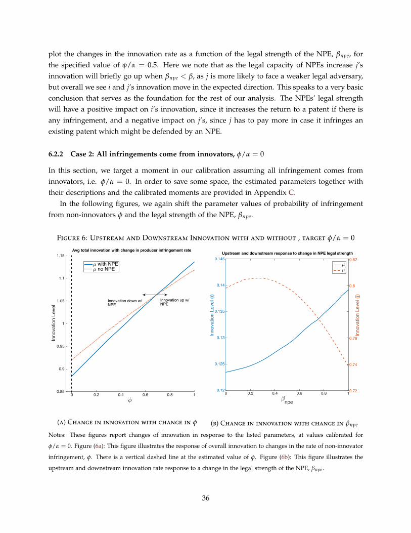
plot the changes in the innovation rate as a function of the legal strength of the NPE, βnpe, forthe specified value of φ/α = 0.5. Here we note that as the legal capacity of NPEs increase j’sinnovation will briefly go up when βnpe < β, as j is more likely to face a weaker legal adversary,but overall we see i and j’s innovation move in the expected direction. This speaks to a very basicconclusion that serves as the foundation for the rest of our analysis. The NPEs’ legal strengthwill have a positive impact on i’s innovation, since it increases the return to a patent if there isany infringement, and a negative impact on j’s, since j has to pay more in case it infringes anexisting patent which might be defended by an NPE.

6.2.2 Case 2: All infringements come from innovators, φ/α = 0

In this section, we target a moment in our calibration assuming all infringement comes frominnovators, i.e. φ/α = 0. In order to save some space, the estimated parameters together withtheir descriptions and the calibrated moments are provided in Appendix C.

In the following figures, we again shift the parameter values of probability of infringementfrom non-innovators φ and the legal strength of the NPE, βnpe.

Figure 6: Upstream and Downstream Innovation with and without , target φ/α = 0

?0 0.2 0.4 0.6 0.8 1

Inno

vatio

n Le

vel

0.85

0.9

0.95

1

1.05

1.1

1.15Avg total innovation with change in producer infringement rate

7 with NPE7 no NPE

Innovation up w/NPE

Innovation down w/NPE

(a) Change in innovation with change in φ

-npe

0 0.2 0.4 0.6 0.8 1

Inno

vatio

n Le

vel (

i)

0.12

0.125

0.13

0.135

0.14

0.145Upstream and downstream response to change in NPE legal strength

Inno

vatio

n Le

vel (

j)

0.72

0.74

0.76

0.8

0.827

i7

j

(b) Change in innovation with change in βnpe

Notes: These figures report changes of innovation in response to the listed parameters, at values calibrated for

φ/α = 0. Figure (6a): This figure illustrates the response of overall innovation to changes in the rate of non-innovator

infringement, φ. There is a vertical dashed line at the estimated value of φ. Figure (6b): This figure illustrates the

upstream and downstream innovation rate response to a change in the legal strength of the NPE, βnpe.

36

The overall changes in innovation efforts in response to the underlying changes in φ and βnpe

look very similar to Figures 5a and 5b. Just like in Case 1, the overall innovation effort declineswhen there are NPEs in the market. The effect when there are no non-innovating infringers ismore pronounced, as innovation drops by 4 percentage points. This is again due to the fact thatNPEs discourage follow-on innovations when there is an associated risk of infringement.

6.2.3 Case 3: Innovators contribute to none of the infringement, φ/α = 1

In this section, we target values such that all of the infringement comes from non-innovators, i.e.φ/α = 1. The estimated parameters together with their descriptions are provided in AppendixTable B3 and the matched moments are described in Appendix Table B4.

Figure 7: Upstream and Downstream Innovation with and without NPE, target φ/α = 1

?0 0.2 0.4 0.6 0.8 1

Inno

vatio

n Le

vel

0.85

0.9

0.95

1

1.05Avg total innovation with change in producer infringement rate

7 with NPE7 no NPE

(a) Change in innovation with change in φ

-npe0 0.2 0.4 0.6 0.8 1

Inno

vatio

n Le

vel (

i)

0.13

0.14

0.15Upstream and downstream response to change in NPE legal strength

Inno

vatio

n Le

vel (

j)

0.82

0.83

0.84

0.857i7j

(b) Change in innovation with change in βnpe

Notes: These figures report changes of innovation in response to the listed parameters, at values calibrated for

φ/α = 1. Figure (7a): This figure illustrates the response of overall innovation to changes in the rate of non-innovator

infringement, φ. There is a vertical dashed line at the estimated value of φ for this targeted value. Figure (7b): This

figure illustrates the upstream and downstream innovation rate response to a change in the legal strength of the NPE,

βnpe.

We see from Figures 5a, 6a, and 7a that when most infringement comes from non-innovatingfirms, i.e. φ ≈ 1, NPEs have an overall positive impact on innovation. This makes intuitive sense

37

because here NPEs increase ex-ante incentives of upstream firms but doesn’t reduce downstreaminnovation. However, as we can see from Figures 5a and 6a, if most infringement is due toinnovators (φ ≈ 0), then NPEs have an overall negative impact on innovation. Further researchon the proportion of infringement due to firms in the process of innovating versus copycats couldhelp us clarify which world we are in.15

Our results from these three exercises indicate that the implications of the effect of NPEs onoverall innovation boil down to the following question: how prevalent are non-innovating firmsin infringement? If most of the infringement is due to non-innovators, the NPEs’ role is that ofprotecting innovators and will tend to increase innovation. If most of the infringement comesfrom innovators, the NPEs could slow overall innovation, although not by a great deal accordingto our calibration. Our results provide preliminary evidence on these distinguishing factors in ageneral equilibrium setup. Further research should focus on the degree to which infringers aresolely producers or in fact innovators themselves.

7 Conclusion

What do non-practicing entities do, and how do they impact innovation and technologicalprogress? Despite the heated debates on this issue in both academic and policy circles, thedirect evidence on their business models is quite limited. In this paper, we attempt to answerthese questions both empirically and theoretically.

On the theoretical side, the model provides new insights into how NPEs operate. In linewith standard approaches, the model allows for NPEs to purchase patents and license themto other firms without using those patents for production. Our model highlights two crucialroles for the NPEs: First, they can purchase patents that are more litigation-prone and use themto threaten other firms to extract more licensing revenue. While this is commonly associatedwith “trolling,” there is a positive contribution of this role: NPEs create value by defendingthe intellectual property of small firms who do not have sufficient means to defend their patents.While this protection incentivizes small firms to innovate more, the same action discourages largefirms who might be infringing on small firm patents. The second role of the NPEs have been asmiddleman in the market for patents, which suffer deeply from informational asymmetry. Byhaving access to the full broker network around the country, NPEs can allocate patents to betterusers.

The elements in our model allow us to come up with a number of relevant and testableimplications. We are able to evaluate these predictions by examining transaction-level data fromlarge NPEs for the first time. We find that NPEs buy non-core patents from smaller originatingentities, and especially litigation-prone patents. They pay more for patents that come from large

15Also note that the innovation from j, µj, is very unresponsive to changes in βnpe. This is because in targetingφ/α = 1 (and matching φ/α = 0.97) we get only a very small probability that j will infringe i as the targeted value forτ = 0.03.

38

firms and for those that are more core to the seller’s business. On the licensing side, NPEs attainhigher fees for those patents that have smaller distance to the licensee. We also find that citationsto NPE-held patents decline around the time of acquisition. This effect is not significant for lowvalue patents, but is most pronounced for those with higher value.

In our final exercise, we calibrate the model to attempt to estimate a net effect of NPEs oninnovation. A crucial component of the model is the amount of patent infringement due to inno-vators and that due to producers who do not innovate. If a large amount of infringement comesfrom non-innovating producers, NPEs have a positive effect on innovation. If most infringementcomes from downstream producers, NPEs generate a net negative effect.

We believe that both the framework and new facts put forth in this paper can shed light on thedebate of the role of NPEs for overall innovation. The welfare and innovation consequences ofNPEs is a policy issue that continues to be relevant and much additional work is needed on thiscrucial topic. Our paper suggests further exploration is warranted. For instance, one importantaspect noted in this paper is the degree to which infringement comes from producing entities asopposed to those who both produce and innovate. Another area is the degree to which infringe-ment truly hampers the capability of small firms to protect their technology. We hope this papercan help provide a foundation for further research on these topics as intellectual property and itssecondary market remain central to discussions of innovation.

References

Abrams, D. S., U. Akcigit, and J. Grennan: 2018, ‘Patent Value and Citations: Creative Destructionor Strategic Disruption?’. Working Paper.

Abrams, D. S. and B. Sampat: 2019, ‘Drug Patent Citations and Value’. Working Paper.

Acemoglu, D., U. Akcigit, H. Alp, N. Bloom, and W. Kerr: 2018, ‘Innovation, Reallocation, andGrowth’. American Economic Review 108(11), 3450–91.

Aghion, P. and P. Howitt: 1992, ‘A Model of Growth Through Creative Destruction’. Econometrica60(3), 323–351.

Ahmadpoor, M. and B. Jones: 2017, ‘The Dual Frontier: Patentable Inventions and Prior ScientificAdvance’. Science 357(6351), 583—587.

Akcigit, U., M. A. Celik, and J. Greenwood: 2016, ‘Buy, Keep, or Sell: Economic Growth and theMarket for Ideas’. Econometrica 84(3), 943–984.

Akcigit, U., J. Grigsby, and T. Nicholas: 2017, ‘The Rise of American Ingenuity: Innovationand Inventors of the Golden Age’. Technical report. National Bureau of Economic ResearchWP23047.

39

Akcigit, U. and W. R. Kerr: 2018, ‘Growth through Heterogeneous Innovations’. Journal of PoliticalEconomy 126(4), 1374–1443.

Allison, J. R., M. A. Lemley, and J. Walker: 2009, ‘Extreme Value or Trolls On Top?The Character-istics of the Most-Litigated Patents’. University of Pennsylvania Law Review 158.

Allison, J. R., M. A. Lemley, and J. Walker: 2011, ‘Patent Quality and Settlement Among RepeatPatent Litigants’. Georgetown Law Journal 99(6777), 12.

Ashtor, J. H., M. J. Mazzeo, and S. Zyontz: 2013, ‘Patents at Issue: The Data behind the PatentTroll Debate’. George Mason Law Review 21, 957.

Benhabib, J., J. Perla, and C. Tonetti: 2014, ‘Catch-up and Fall-back through Innovation andImitation’. Journal of Economic Growth 19(1), 1–35.

Bessen, J. E. and M. J. Meurer: 2014, ‘The Direct Costs from NPE Disputes’. 99 Cornell Law Review387.

Bloom, N., M. Schankerman, and V. R. John: 2013, ‘Identifying Technology Spillovers and ProductMarket Rivalry’. Econometrica 81(4), 1347–1393.

Bloom, N. and J. Van Reenen: 2002, ‘Patents, Real Options and Firm Performance’. The EconomicJournal 112(478), C97–C116.

Blundell, R., R. Griffith, and J. Van Reenen: 1999, ‘Market Share, Market Value and Innovation ina Panel of British Manufacturing Firms’. Review of Economic Studies 66(3), 529–554.

Caballero, R. and A. Jaffe: 1993, ‘How High are the Giants’ Shoulders: An Empirical Assessmentof Knowledge Spillovers and Creative Destruction in a Model of Economic Growth’. NBERMacroeconomics Annual 8(1), 15–86.

Chatterjee, S. and E. Rossi-Hansberg: 2012, ‘Spinoffs and the Market for Ideas’. InternationalEconomic Review 53(1), 53–93.

Chien, C.: 2014, ‘Startups and Patent Trolls’. Stanford Technology Law Review 17:461.

Cohen, L., J. M. Golden, U. G. Gurun, and S. D. Kominers: 2017, ‘Troll Check: A Proposal forAdministrative Review of Patent Litigation’. Boston University Law Review 97, 1775.

Cohen, L., U. G. Gurun, and S. D. Kominers: 2016, ‘The Growing Problem of Patent Trolling’.Science 352(6285), 521–522.

Cohen, L., U. G. Gurun, and S. D. Kominers: 2018, ‘Patent Trolls: Evidence from Targeted Firms’.Management Science. forthcoming.

Cotropia, C. A., J. P. Kesan, and D. L. Schwartz: 2014, ‘Unpacking Patent Assertion Entities(PAEs)’. Minnesota Law Review 1571, 99.

40

Czarnitzki, D. and A. A. Toole: 2011, ‘Patent protection, Market Uncertainty, and R&D Invest-ment’. The Review of Economics and Statistics 93(1), 147–159.

Eaton, J. and S. Kortum: 1996, ‘Trade in Ideas: Patenting and Productivity in the OECD’. Journalof International Economics 40(3), 251—278.

Feldman, R. and M. A. Lemley: 2015, ‘Do Patent Licensing Demands Mean Innovation?’. IowaLaw Review 101:137.

Feng, J. and X. Jaravel: 2017, ‘Crafting Intellectual Property Rights: Implications for Patent As-sertion Entities, Litigation, and Innovation’. LSE Working Paper.

Fischer, T. and J. Henkel: 2012, ‘Patent Trolls on Markets for Technology: An Empirical Analysisof NPEs Patent Acquisitions’. Research Policy 41, 9.

Galasso, A. and M. Schankerman: 2015, ‘Patents and Cumulative Innovation: Causal Evidencefrom the Courts’. Quarterly Journal of Economics 130(2), 317–369.

Galasso, A., M. Schankerman, and C. J. Serrano: 2013, ‘Trading and Enforcing Patent Rights’.RAND Journal of Economics 44.

Garicano, L., C. Lelarge, and J. Van Reenen: 2016, ‘Firm Size Distortions and the ProductivityDistribution: Evidence from France’. American Economic Review 106(11), 3439—3479.

Graham, S., A. Marco, and R. Miller: 2015, ‘The USPTO patent examination research dataset: Awindow on the process of patent examination’.

Griffith, R., S. Redding, and J. Van Reenen: 2003, ‘R&D and Absorptive Capacity: Theory andEmpirical Evidence’. Scandinavian Journal of Economics 105(1), 99–118.

Griffith, R., S. Redding, and J. Van Reenen: 2004, ‘Mapping the Two Faces of R&D: ProductivityGrowth in a Panel of OECD Industries’. Review of Economics and Statistics 86(4), 883–895.

Grossman, G. M. and E. Helpman: 1991, ‘Quality Ladders in the Theory of Growth’. Review ofEconomic Studies 29(4), 43–61.

Haber, S. H. and S. H. Werfel: 2015, ‘Why Do Inventors Sell to Patent Trolls? ExperimentalEvidence for the Asymmetry Hypothesis’. Stanford University Working Paper.

Haber, S. H. and S. H. Werfel: 2016, ‘Patent Trolls as Financial Intermediaries? ExperimentalEvidence’. Economics Letters 149, 64–66.

Hall, B. H., A. B. Jaffe, and M. Trajtenberg: 2001, ‘The NBER Patent Citations Data File: Lessons,Insights and Methodological Tools’. National Bureau of Economic Research Working Paper no:8498.

41

Henderson, R., A. Jaffe, and M. Trajtenberg: 1998, ‘Universities as a Source of Commercial Tech-nology: A Detailed Analysis of University Patenting, 1965Ð1988’. Review of Economics andStatistics 80(1), 119–127.

Jaffe, A. and M. Trajtenberg: 1999, ‘International Knowledge Flows: Evidence From Patent Cita-tions’. Economics of Innovation and New Technology 8(1-2), 105–136.

Jaravel, X., N. Petkova, and A. Bell: 2018, ‘Team-Specific Capital and Innovation’. AmericanEconomic Review 108, 1034–1073.

Kempf, E. and O. Spalt: 2018, ‘Litigating Innovation: Evidence from Securities Class ActionLawsuits’. University of Chicago, Booth School of Business Working Paper.

Khan, B. Z.: 2014, ‘Trolls and Other Patent Inventions: Economic History and the Patent Contro-versy in the Twenty-first Century’. George Mason Law Review 21, 825.

Khan, B. Z.: 2015, ‘Inventing Prizes: A Historical Perspective on Innovation Awards and Tech-nology Policy’. Business History Review 89(4), 631–660.

Kiebzak, S., G. Rafert, and C. E. Tucker: 2016, ‘The Effect of Patent Litigation and Patent AssertionEntities on Entrepreneurial Activity’. Research Policy 45(1), 218–231.

Klette, T. and S. Kortum: 2004, ‘Innovating Firms and Aggregate Innovation’. Journal of PoliticalEconomy 112(5), 986–1018.

Konig, M., J. Lorenz, and F. Zilibotti: 2016, ‘Catch-up and Fall-back through Innovation andImitation’. Theoretical Economics 11(3), 1053–1102.

Kortum, S.: 1997, ‘Research, Patenting, and Technological Change’. Econometrica 65(6), 1389—1419.

Lai, R., A. D’Amour, and L. Fleming: 2009, ‘The Careers and Co-authorship Networks of USPatent-holders, since 1975’. Unpublished Working Paper, Harvard University.

Lamoreaux, N. R. and K. L. Sokoloff: 1999, ‘Inventors, Firms, and the Market for Technologyin the Late Nineteenth and Early Twentieth Centuries’. Learning by Doing in Markets, Firms,and Countries. ed. by N. R. Lamoreaux, D. M. G. Raff, and P. Temin, pp. 19–60. University ofChicago Press.

Lanjouw, J. and M. Schankerman: 2001, ‘Characteristics of Patent Litigation: A Window onCompetition’. RAND Journal of Economics 32, 1.

Lemley, M. A. and R. Feldman: 2016, ‘Patent Licensing, Technology Transfer, and Innovation’.American Economic Review, Papers and Proceedings 106(5), 188–92.

42

Lentz, R. and D. T. Mortensen: 2008, ‘An Empirical Model of Growth through Product Innova-tion’. Econometrica 76(6), 1317–1373.

Lu, J.: 2012, ‘The Myths and Facts of Patent Troll and Excessive Payment: Have Non-PracticingEntities (NPEs) Been Overcompensated?’. Business Economics 47:4.

Marco, A. C. and R. Miller: 2017, ‘Patent Examination Quality and Litigation: Is There a Link?’.

Nicholas, T.: 2013, ‘Are Patents Creative or Destructive?’. Antitrust Law Journal 79, 405–421.

Pènin, J.: 2012, ‘Strategic Uses of Patents in Markets for Technology: A Story of Fabless Firms,Brokers and Trolls’. Journal of Economic Behavior and Organization 84(6334), 1.

Perla, J. and C. Tonetti: 2014, ‘Equilibrium Imitation and Growth’. Journal of Political Economy122(1), 52—76.

Reitzig, M., J. Henkel, and F. Schneider: 2010, ‘Collateral Damage for R&D Manufacturers: HowPatent Sharks Operate in Markets for Technology’. Industrial and Corporate Change 19, 3.

Risch, M.: 2012, ‘Patent Troll Myths’. Seton Hall Review 42:457.

Rivette, D. and K. Klein: 2000, ‘Discovering New Value in Intellectual Property’. Harvard BusinessReview.

Schwartz, D. L. and J. P. Kesan: 2014, ‘Analyzing the Role of Non-Practicing Entities in the PatentSystem’. Cornell Law Review 99:2.

Serrano, C.: 2010, ‘The Dynamics of Transfer and the Renewal of Patents’. RAND Journal ofEconomics 41(4), 686—708.

Serrano, C.: 2018, ‘Estimating the Gains from Trade in the Market for Patent Rights’. InternationalEconomic Review 41(4), 686—708. forthcoming.

Shrestha, S. K.: 2010, ‘Trolls or Market-Makers?’. An Empirical Analysis of Nonpracticing Entities.Columbia Law Review 110, 1.

Simonds, W. E.: 1871, Practical Suggestions on the Sale of Patents. Connecticut: Self-Published.

Toole, A. A. and C. Turvey: 2009, ‘How Does Initial Public Financing Influence Private Incentivesfor Follow-on Investment in Early-stage Technologies?’. Journal of Technology Transfer 34, 43–58.

Tucker, C.: 2014, ‘Patent Trolls and Technology Diffusion : The Case of Medical Imaging’. Work-ing Paper.

43

A Data and Variable Descriptions

A.1 Data Cleaning and Merging

A.1.1 Company Name Cleaning

In order to aggregate patents produced by or sold to the same entities properly, it is critical tohave a way to clean company names, which we discuss here. Our approach is similar to thatused in the NBER Patent Database Project (PDP), but we extend past the 2006 end date of thatdata set.16

Company identifiers used by the USPTO are known to contain serious flaws. The most recentefforts to harmonize the company names do not take many issues into account. In particular, thesame firms are assigned to different identifiers whenever there is a change to their legal status(e.g. “MONSANTO TECHNOLOGY LLC”, “MONSANTO TECHNOLOGY LLP”).

In order to tackle the flaws generated by USPTO identifiers, we employ a conservative com-pany name cleaning algorithm, so that assignee identifier flaws are minimized. The main ideabehind the cleaning algorithm is to clean all unnecessary company indicators and company typeabbreviations. If the resulting string variables are the same, the algorithm assigns the same as-signee identifier to each modified string. The same algorithm is used to clean licensee names inND.

The algorithm can be summarized as follows:1.All letters of the string are made upper case.2.Any part of the string coming after a first comma is deleted.3.All non-alphanumeric characters are deleted.4.The first 3 characters of the string are deleted if it starts with “THE”.5.The company indicators such as CO, CORP, LLC, etc are removed.6. If the resulting string has zero length, the original string is used. (e.g. “ABCO, INC” ,

“COCO,INC”)

A.1.2 Data Merging

The PAB, LM, INV, and ND datasets are merged on patent number.17 We keep only utility patentsand drop those with application dates before 1987.18 We keep patents assigned to individuals ifthe number of listed inventors is one. This is due to the difficulty in calculating portfolios for

16We would like to thank Murat Alp Celik for sharing his cleaning algorithm.17 We complement our data with recently announced citation and claim decomposition data. It can be found at the

following link: http://www.patentsview.org/download.18 More than 99 percent of NPE patents were applied for after 1987. This is the main reason that we focus on

post-1987 patents.

44

ever-changing assignee groups of multiple inventors. Thus, small, unincorporated groups areomitted from the analysis.

We keep only patents in technology categories (three-digit IPC) where the NPEs operate. Wemerge USPTO classes and IPC classes and use IPC classes in our analysis.19 Each patent in PABis matched with harmonized assignee identifiers.20 The company name cleaning algorithm isused on assignee and licensee names from the ND data. We match licensees with PAB data andkeep those for which there is patent data. We drop patents with missing distance to originatingentity and litigation risk from the acquisition deals.

A.2 Variable Construction

A.2.1 Lifetime Citations

We construct a lifetime forward citation variable for each patent to account for the fact thatpatents are different ages, and therefore have differing amounts of time to accumulate citation.

In order to construct this measure, the mean forward citations-patent age relationship isconstructed for each technological category. We calculate lifetime citations by inflating the totalcitations already received by the ratio of the total mean citations of the same technology classdivided by the mean for the average patent of the same age and technology class. While thisprocedure will understate the number of lifetime citations for any patent that has zero in ourdata set, the mean number of lifetime cites should still be correct.

The procedure is applied to all patents granted after 1976 using technology categories in Hallet al. (2001). Note that we limit our attention to patents with application year after 1987 in thefinal analysis.

A.2.2 Acquisition Price

The patents are purchased in bundles of firms at a given cost. We deflate this cost to real 2010dollars. For our deal-level analysis, e.g. Table 3, some patent bundles combine patents that arenot part of our analysis with those that are (e.g. we do not use international patents). In thiscase, we adjust the acquisition cost by the revenue weights representative of the overall outsideand inside sample. For instance, if international patents are on average worth 1/5 of a US patentin the sample, we assign in the deal 5/6 of the cost to the patent in the sample for every 1/6assigned to international patent.

A.2.3 Lifetime Revenue

As with citations, it is necessary to calculate a single revenue number so that we may comparepatents of different ages. We begin with per-patent annual nominal revenue numbers and use the

19See http://www.uspto.gov/web/patents/classification for further information.20Found at http://www.uspto.gov/web/offices/ac/ido/oeip/taf/data/misc/data_cd.doc/assignee_harmonization/cy2014

45

CPI to deflate them to real 2010 dollars. For each technology category, a mean revenue-patentage relationship is constructed. The lifetime revenue of a patent is estimated by inflating theobserved cumulative revenue by the ratio of the mean lifetime revenue to the mean cumulativerevenue for patents of the same age (by technology category). We then normalize all revenueamounts so that total lifetime revenue is 200 in order to maintain the confidentiality.

Occasionally, patents generate licensing revenue after expiration (since they may still generateincome from prior infringement). In this case, no normalization procedure is used and theobserved real revenue is simply summed. Since patents may also generate revenue prior to grant(in anticipation of grant), we begin observing revenue at the first filing date (which is the sameas application date for 90 percent of patents). That is, patent age is defined as the differencebetween revenue generation year and first filing year. If a patent realizes revenue while classifiedas abandoned, lapsed, or inactive, it is simply added to the normalized real revenue.

A.2.4 Distance

In order to quantify the distance between two technology classes, we define distance as in Akcigitet al. (2016), using the first 2 digit IPC to denote a technology class:

d(X, Y) ≡ 1− #(X⋂

Y)#(X

⋃Y)

, with 0 ≤ d(X, Y) ≤ 1.

where #(X⋂

Y ) denotes the number of patents that cite technology classes X and Y together,and #(X

⋃Y) denotes the number of patents which cite X or Y or both.

Also following Akcigit et al. (2016), we construct a patent-to-entity distance metric. Thedistance of a patent p to an entity f ’s patent portfolio is calculated by averaging the distance ofp to each patent in entity f ’s patent portfolio as follows.

dι(p, f ) ≡

1||Pf || ∑

p′∈Pf

d(Xp, Yp′)ι

1ι

Where 0 < ι < 1, and where 0 ≤ dι(p, f ) ≤ 1. Note that Pf represents the set of all patentsthat were invented by entity f prior to patent p, ||Pf || denotes the cardinality of the set, andd(Xp, Yp′) measures the distance between technology classes of patents p and p′.

We set ι = 23 for our baseline results. Using the measure above, we constructed two different

distance measures: distance to originating entity and distance to licensee.

A.2.5 Litigation Risk

To estimate the likelihood a patent may be involved in litigation, we use the linear probabilitymodel developed in Lanjouw and Schankerman (2001):

ILitigatedi,j,t = ζ + ηi + δt + φ× COi,j,t + εi,j,t (18)

46

Where the dependent variable is a dummy variable equaling 1 if the patent is ever litigatedor a complaint is ever filed, and 0 otherwise, and (i,j,t) represent patent, technology category,and application year, respectively. ηi is a firm fixed effect and δt the application year fixed effect.COi,j,t is a vector of covariates, and εi,j,t is the error.

Our model is motivated by Lanjouw and Schankerman (2001), but we include the followingadditional variables: examiner backward and forward citation percent, growth of technology cat-egories, and entity fixed effects. We omit indicator variables for entity types (such as individualinventors, foreign firms operating in the U.S., and firms operating in the U.S., which were in theoriginal model).

We estimate the model on the full dataset and then predict litigation risk for each patent.Robust standard errors are clustered at originating entity level.

B Additional Tables and Figures

B.1 Deal-level Summary Statistics

Table A1 reports deal-level summary statistics on all deals through which the NPEs acquiredpatents from 2003 - 2014. Compared to Table 1, which reported patent level statistics, the averageentity size is substantially smaller, indicating that the acquisitions from smaller firms are morenumerous and have a smaller average deal size. In fact, deals from individual inventors represent17% of total deals, over an order of magnitude higher than the share of individual inventors in thepatent universe. Deals with individual inventors and small firms accounts combined accountsfor fully two-thirds of the total acquisition deals. Only 5% of patent acquisition deals are struckwith large originating firms.

The mean number of forward citations is substantially higher in Table A1 than Table 1, whileage is lower, indicating that smaller firms are likely selling newer, more highly cited patents.Larger firms are most likely selling NPEs larger numbers of older, less-cited patents. Deal sizeis right-skewed, with a small number of very large deals driving the mean up substantially; themedian acquisition deal involves only 4 patents. Age here is defined as the acquisition date minusapplication date, and has a mean of just over 7 years. The deal acquisition price is normalized sothat the mean is 200. We first divide the acquisition prices of the deals by the number of patentsinvolved. Then, we normalize this value so that mean is 200. Finally, we multiply the normalizedvalues per deal with the number of patents involved to construct normalized acquisition pricesfor each deal.

B.2 Patent-level Summary Statistics

Table A2 reports patent-licensee-year level summary statistics derived from NPE licensing dealdata from 2008 to 2014. The licensee is the ultimate end-user of the patent; most patents in thedataset have multiple licensees. It is immediately apparent that the mean distance to licensee is

47

Table A1: Patent Acquisition Deal Summary Statistics

Variables Mean p25 p50 p75 SdDistance to Originating Entity 0.32 0 0.29 0.53 0.28Originating Patent Portfolio Size 762.56 2.31 6.54 200.40 2896.74Log Originating Patent Portfolio Size 3.07 0.84 1.88 5.30 2.76Litigation Risk 13.22 8.57 11.61 15.43 8.73Individual Inventor 0.17 0 0 0 0.37Total Claims 22.09 14.72 20 27 11.44Lifetime Forward Citations 42.68 10.13 21.28 46.31 66.74Backward Citations 20.11 6.34 10.57 20.67 30.98Hotness 30.68 13.46 27.94 42.90 22.59Deal Size 23.10 2 4 13 98.84Age 7.09 4 7.11 10 4.27Log Acquisition Price 5.91 4.99 5.85 6.74 1.27

Notes: Acquisition deal-level data from 2003 - 2014 includes all NPE patent acquisition deals in the U.S.

about 50% larger than the mean distance to originating entity (Table 1 and A1). This may leadone to believe that the reallocation of patents from originator to licensee via NPEs is inefficient,insofar as it increases the mean patent distance and thus usefulness of a patent to a firm. Thisconclusion would be unjustified, as the distance metric is an increasing function of firm size(Figure B1), and the mean licensee size is several times larger than originating entity size. Thecorrect comparison would be the mean empirical distance to licensee (0.47) versus the meandistance for a randomly chosen set of patents in the licensee’s portfolio. The mean distance forthe randomly chosen patents to the licensee portfolios is 0.64, which shows that the NPE-licensedpatents have substantially smaller distances from the licensees than average.

Returning to Table A2, we see that, as with originating entity size, the licensee size is alsoright-skewed. Licensee size is the number of patents (including subsequently granted applica-tions) in the licensee’s portfolio at the time of the licensing deal. Because data in Table A2 isaggregated at the patent-licensee-year level, a direct comparison with Tables 1 and A1 is com-plicated, but most of the variable means are similar. Patent age, with a mean and median ofaround 12, is defined as the duration between application date and licensing date. We have seensome suggestive findings from the summary statistics; we now make use of regressions to furtherinvestigate the impact of NPEs on innovation markets.

B.3 Additional Figures

We noted in the discussion of Table A2 how the distance measure is correlated with firm size.Here we plot a scatter of the relationship to illustrate it is indeed the case.

48

Table A2: Licensing Transaction Summary Statistics

Variables Mean p25 p50 p75 SdDistance to Licensee 0.47 0.23 0.45 0.71 0.30Distance of Random Patent to Licensee 64.35 33.38 76.77 93.49 33.34Licensee Patent Portfolio Size 5095.57 64 867 5347 9120.51Log Licensee Patent Portfolio Size 6.19 4.16 6.77 8.58 3.01Litigation Risk 11.85 6.93 10.40 14.62 8.61Individual Inventor 0.06 0 0 0 0.25Total Claims 19.30 10 17 24 15.22Lifetime Forward Citations 31.34 3.46 11.34 32.86 60.32Backward Citations 22.64 4 8 17 52.40Hotness 32.07 2.56 25 50 29.97Age 11.98 8 12 15 5.15Log Licensing Fee*** 8.25 6.28 8.04 10.33 2.48

Notes: Patent-Licensee-Year level data includes all NPE licensing transactions from 2008 - 2014. Please see the textand Appendix A.2 for variable definitions and normalization.

Figure B1: Distance and Originating Entity Size

020

4060

8010

0D

ista

nce

0 5 10Originating Entity Size

Notes: This figure shows the relationship between firm size and mean patent distance for patents sold to NPEs. Largerfirms on average sell more distant patents.

C Calibration

Here we report the calibrated values for when we targeted φ/α = 0 and φ/α = 1. The figuresfrom our selected exercises can be found in Section 6, Figures 6 and 7.

49

Table B1: Parameter Values, target φ/α = 0

Parameter Description Value Main Identification

— Panel A. External Calibration —

η R&D cost scaling for external innovation 0.25 Akcigit and Kerr (2018)

ξ Convexity of R&D cost 2 Akcigit and Kerr (2018)

E[di] Expected distance of upstream to NPE 0.30 NPE Distribution

E[dk] Expected distance of downstream to NPE 0.50 Taken in uniform[0,1]

— Panel B. Internal Calibration —

Ω Profit of Licensing Entity 3.80 Correlation of prices

π Profit of Innovating Entity 0.11 Correlation between pi and di

φ Probability producer infringement 0 Pr producer infringement

τ Probability innovator infringement 0.88 Pr producer infringement

β Probability of Winning (Upstream) 0.34 Correlations, Prices

βnpe Probability of Winning in Court (NPE) 0.94 Prices

κ Max. Search Cost 2.25 Pr(sale)Notes: All parameters are estimated jointly.

Table B2: Moments, target φ/α = 0

Moment Data Model

Price upstream producer sells to NPE 1 1

Average Price NPE sells to downstream 1.54 1.54

Correlation between distance of upstream to NPE and price -0.07 -0.07

Correlation between price sold and bought from NPE 0.37 0.37

Innovation intensity of downstream innovator 0.74 0.74

Probability of sale to NPE 0.23 0.23

Proportion of infringement from non-innovators 0 0.01

50

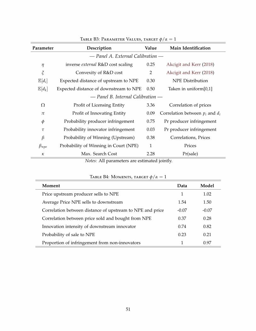
Table B3: Parameter Values, target φ/α = 1

Parameter Description Value Main Identification

— Panel A. External Calibration —

η inverse external R&D cost scaling 0.25 Akcigit and Kerr (2018)

ξ Convexity of R&D cost 2 Akcigit and Kerr (2018)

E[di] Expected distance of upstream to NPE 0.30 NPE Distribution

E[dk] Expected distance of downstream to NPE 0.50 Taken in uniform[0,1]

— Panel B. Internal Calibration —

Ω Profit of Licensing Entity 3.36 Correlation of prices

π Profit of Innovating Entity 0.09 Correlation between pi and di

φ Probability producer infringement 0.75 Pr producer infringement

τ Probability innovator infringement 0.03 Pr producer infringement

β Probability of Winning (Upstream) 0.38 Correlations, Prices

βnpe Probability of Winning in Court (NPE) 1 Prices

κ Max. Search Cost 2.28 Pr(sale)Notes: All parameters are estimated jointly.

Table B4: Moments, target φ/α = 1

Moment Data Model

Price upstream producer sells to NPE 1 1.02

Average Price NPE sells to downstream 1.54 1.50

Correlation between distance of upstream to NPE and price -0.07 -0.07

Correlation between price sold and bought from NPE 0.37 0.28

Innovation intensity of downstream innovator 0.74 0.82

Probability of sale to NPE 0.23 0.21

Proportion of infringement from non-innovators 1 0.97

51

D Theoretical Appendix

This section more explicitly derives the predictions of the model. We first write out some objectsand prices in the economy that we will reference in our derivations.

Pr (sale) =pi,npe −Vkeep

iκ

(19)

pi,npe =Vkeep

i + Vnpe

2(20)

pnpe,j =βnpeΩj

2(21)

pnpe,k =Ωk (1− dk)

2(22)

pi,j = βiπ (1− di) +βiΩj

2(23)

Vprodi = π (1− di) .

Vkeepi = αpi,j + (1− α)Vprod

i

= αβi

[π (1− di) +

Ωj

2

]+ (1− α)π (1− di) .

(24)

Vnpe = αpnpe,j + (1− α) pnpe,k (25)

D.1 Derivation of Prediction 1

The NPE is more likely to buy patents from small firms. Moreover, this effect is more pronounced forlitigation-prone patents

∂

∂qiPr (sale) = −β′(qi)α

2κ

[π (1− di) +

Ωj

2

]< 0.

With probability of sale given in Equation 19, we plug in Equation 20. In order to fullycharacterize, we then use Equations 24 and 25:

Pr (sale) =Vnpe −Vkeep

i2κ

=αpnpe,j + (1− α) pnpe,k − αpi,j − (1− α)π (1− di) .

2κ

52

Plug in Equations 21, 22, and 23 to get the probability of sale as a function of exogenousvariables with respect to i.

Pr (sale) =α

βnpeΩj2 + (1− α) Ωk(1−dk)

2 − α(

βiπ (1− di) +βiΩj

2

)− (1− α)π (1− di)

2κ(26)

∂

∂qiPr (sale) = −

α(

β′(qi)π (1− di) +β′(qi)Ωj

2

)2κ

= −αβ′(qi)

2κ

[Ωj

2+ π (1− di)

]We then take the derivative with respect to litigation risk:

∂2

∂α∂qiPr (sale) = −β′(qi)

2κ

(Ωj

2+ π (1− di)

)< 0.

D.2 Derivation of Prediction 2

The likelihood of a patent sale increases as distance of the patent from the initial innovating firm increases.Moreover, this effect is more pronounced for large firms

∂

∂diPr (sale) =

αβiπ + (1− α)π

2κ> 0.

∂2

∂di∂qiPr (sale) =

β′(qi)απ

2κ> 0.

Both of these follow from derivatives of Equation 26 with respect to distance and firm size.

D.3 Derivation of Prediction 3

The NPE pays more for large firms’ patents:

Here we write out the acquisition price from Equation 20 which plugs in Equations 21, 22, 24and 25, which are the values that determine the price:

pi,npe =αβi

[π (1− di) +

Ωj2

]+ (1− α)π (1− di) + α

βnpeΩj2 + (1− α) Ωk(1−dk)

2

2(27)

Now we simply take derivative with respect to qi which shows up through βi

∂pi,npe

∂qi=

β′(qi)α[π (1− di) +

Ωj2

]2

> 0.

53

D.4 Derivation of Prediction 4

The acquisition price decreases as patent distance to the seller increases:

See Equation 27 and take the derivative with respect to distance for i, di–

∂pi,npe

∂di= − [αβi + 1− α]π

2< 0

D.5 Derivation of Prediction 5

The average price that a licensing firm pays to NPEs decreases as the distance to the licensee increases

Recall Equation 22:

pnpe,k =Ωk (1− dk)

2.

The prediction immediately follows from differentiation with respect to dk.

D.6 Ambiguous effect on firm j’s innovation

Here we show how the NPE has an ambiguous effect on firm j’s innovation. Recall:

∆µj = η1

ξ−1 [[Ωj − τE(p.,j)

] 1ξ−1 −

[Ωj − τpi,j

] 1ξ−1 ]

∆µi = η1

ξ−1[E[pi,npe − ε]

] 1ξ−1 − η

1ξ−1[E[Vkeep]

] 1ξ−1

To show the ambiguous effect on µj, it is sufficient to show that for some parameters pnpe,j >

pi,j and for other parameters pnpe,j < pi,j and show that even in these cases i visits the NPE withpositive probability. Recall E(p.,j) = Pr(i uses NPE)× pnpe,j + [1− Pr(i uses NPE)]×E[pi,j]

Plugging in the values for pnpe,j and pi,j, we want to show uncertainty over the relationshipbetween:

βiπ(1−E[di]) +βiΩj

2≶

βnpeΩj

2

We see that for βi = 0 and βnpe > 0 one side of the inequality is confirmed (j will innovateless with the NPE). For βnpe < βi, the other side of the inequality is confirmed (j will innovatemore with the NPE).

We lastly verify there are cases where i goes to the NPE with positively probability even ifβnpe < βi. This can occur when Vnpe > Vkeep

i rewritten as:

αβnpeΩj

2+ (1− α)

Ωk (1− dk)

2> αβi

[π (1− di) +

Ωj

2

]+ (1− α)π (1− di)

54

Assume βnpe = 0 and βi > 0. Note that for certain values of Ωk (1− dk) the inequality of theabove equation will still hold:

(1− α)Ωk (1− dk)

2> αβi

[π (1− di) +

Ωj

2

]+ (1− α)π (1− di)

When di → 0 and dk > 0 we see the result holds for small α. The intuition for this is that imay choose to visit the NPE due to its distance reduction role even if the NPE is worse in courtcapability. Thus j will observe less potential interference. This will only hold for low values ofβnpe, which we do not find in our calibration.

55