#2008-046

To Be or Not to Be at the BOP:A One-North-Many-Souths Model with Subsistence and Luxury Goods

Adriaan van Zon and Tobias Schmidt

(UNU-MERIT, August 2008)

Working Paper Series

United Nations University - Maastricht Economic and social Research and training centre on Innovation and Technology Keizer Karelplein 19, 6211 TC Maastricht, The Netherlands

Tel: (31) (43) 388 4400, Fax: (31) (43) 388 4499, e-mail: info@merit.unu.edu, URL: http://www.merit.unu.edu

2

3

To Be or Not to Be at the BOP: A One-North-Many-Souths Modelwith Subsistence and Luxury Goods

byAdriaan van Zon and Tobias Schmidt

(UNU-MERIT, August 2008)AbstractIn this paper we seek to explain the causes and consequences of Northern penetration in Southernsubsistence markets in order to reach the countless masses at the Bottom of the (Income)Pyramid. To this end we formulate a One-North-Many-Souths model, inspired by the Krugman(1979) North-South model. In our model, Southern countries are differentiated with respect topopulation size, but also the degree of internal connectedness as a proxy for the cost involved inreaching the local subsistence market. Northern subsistence goods production in Southerncountries takes place under increasing returns to scale, why local production of subsistence goodstakes place under constant returns to scale. Using this set-up, we show what kind of Southerncountries would be penetrated first, and under which conditions this would happen. From thepoint of view of Northern producers, Southern countries can be divided into three classes: thebroad class of partner- and non partner countries, and within the class of partner countries, thesub-classes of small and large partners. In this context, small partners are so small, that all oflocal subsistence production is taken over by the North, while in large countries part ofsubsistence consumption must still be met out of local subsistence production. The main insightscoming from numerical simulations with the model are that Northern penetration on Southernmarkets releases (labor) resources that can then be used for producing tradable luxury goods. Thishas a negative terms of trade effect for the South, but a positive income effect, while, moreover,the latter effect tends to outweigh the former. In addition, small partner countries generally standto gain more from Northern penetration than large countries, as in small partner countriesrelatively more resources would be released when shifting production of subsistence goods fromlocal to Northern technologies. Using numerical simulations in which we increase the rate ofimitation, we show that this leads to higher terms of trade for the South, and consequently, ahigher penetration of the North in Southern countries with respect to subsistence production. Thereason is that the opportunity cost of using Northern labor in Northern luxury goods productionfalls, and consequently more Northern labor is allocated to its alternative use of managingsubsistence goods production in Southern countries. Thus we are able to ‘explain’ the recentpenetration of Northern firms in subsistence goods production in countries like India and China(which have become increasingly important as manufacturing trading partners), as the lattercountries are both large in population terms as well as relatively well connected.

JEL-codes: D58,F12,F16,F23,O33.Key words: Bottom of the Pyramid, North-South model, luxury goods, subsistence goods.

UNU-MERIT Working PapersISSN 1871-9872

Maastricht Economic and social Research and training centre on Innovation andTechnology, UNU-MERIT

UNU-MERIT Working Papers intend to disseminate preliminary results of researchcarried out at the Centre to stimulate discussion on the issues raised.

4

5

1. IntroductionMuch of the wealth in the world is concentrated in the hands of relatively few people.

Most of these people are situated in the Western world, i.e. the United States and Europe,

whereas poverty rules in large parts of Africa, Asia and South America. From a demand

point of view, the structure of the world market resembles a pyramid, with a numerically

small but rich part at the top and a much larger but poor part at the bottom. Multinational

corporations have routinely ignored the bottom of the pyramid (henceforth BOP). To some

extent this is because the margins on products sold there are necessarily small, but it is also

because the products affordable by poor buyers are necessarily low-cost products. Indeed,

the cost-price of a product should be just about enough to cover the cost of embedding its

core functional characteristics (i.e. its ‘essence’) into the product, but not enough to

differentiate it from otherwise similar products through carefully designed marketing

campaigns.1 Indeed, many of the high-tech products widely used in Western societies these

days thrive on fleeting product fads. Users of mobile phones, games consoles, cars, kitchen

appliances and even holidays put a high premium on variety and temporary exclusivity and

suppliers happily oblige by providing the variety one is looking for in the product market

niches created by their own marketing activities.

The poor of the world, in contrast, are striving to expand their consumption goods

spectrum largely to cover their basic needs more completely. Because of their low income,

they often fall short of covering the complete basic needs spectrum. However, it may well be

possible to service the basic needs of the poor more completely by selling products that have

been stripped down to the bare functional essentials at prices that enable (nearly) everyone to

obtain these products. In the latter case volumes sold could be practically infinitely high and

even with very small but still positive margins, profits are potentially very large indeed. So, if

products, but also the way in which products are brought to the local market, could be

geared more directly to the needs of the people at the bottom of the income pyramid, both

consumers and producers could gain.

1 Prahalad and Hammond claim that … “It is hard to argue that the wealth of technology and talentwithin leading multinationals is better allocated to producing incremental variations of exisitingproducts than to addressing the real needs- and real opportunities- at the bottom of the pyramid.”(Prahalad and Hammond (2002, p.11)). On this matter, see also Prahalad (2006).

6

The reason why we underline the importance of the way in which products are brought

to the local market is that doing so is intrinsically more difficult in BOP societies than in

Western societies. The latter societies are densely connected through both physical

infrastructure like (rail-) roads, airlines and shipping networks, and a variety of information

and communication channels. In BOP societies, by contrast, such connections are often sorely

lacking. The lack of true mass media and other means of long-distance communication make

it difficult to raise awareness for the existence of a product, since marketing campaigns using

television broadcasts or newspapers are not an option. Instead, advertisement needs to be

explicitly geared towards local, small shop suppliers, cf. Prahalad (2006). The same applies to

actually making the product available. Somewhat perversely, the sparsely connected BOP

societies often bear higher transportation costs than is typically the case in Western societies,

while these same societies can ill afford to pay these higher costs.

To illustrate the working of the main principles involved, we construct a model that

distinguishes between a rich North and a poor South, in the tradition of Krugman (1979), but

also Helpman (1993) and Grossman and Helpman (1991) and many others since, cf. Chui c.s.

(2002) for an overview. Unlike Krugman (1979), in our model the South consists of many

countries that differ both in population size and in ‘connectedness’, a catch-all that represents

the cost of reaching the market and can stand for both the density of the transportation

network as well as those used for (tele-) communication. Again unlike Krugman (1979), we

subdivide the goods produced into two main groups, one homogeneous subsistence good

and a multitude of luxury goods. Furthermore, we will make the assumption that

consumption of the subsistence good at the subsistence level generates a zero level of utility,

while subsistence good consumption over and above subsistence level yields no additional

utility. For luxury goods we assume that any positive level of consumption generates positive

utility in a Love of Variety way (cf. Krugman (1979)). This implies that the relative demand

for goods and services in rich countries will be tilted towards luxury goods, and the other

way around in poor countries, ceteris paribus. The demand structure for a Southern country

is highlighted in Figure 1 below. It resembles a structure with different income-elasticities for

subsistence and luxury goods as implied by the use of non-homothetic utility functions as in

Matsuyama (2000), for example. However, in our case, we can keep the model relatively

simple by assuming two modes of operandi for demand: the case where actual income is

7

below subsistence income, and no luxury goods will be demanded, and the other case in

which free disposable income (the excess of actual income over subsistence income) is spent

on luxury goods.

In this Figure, the utility function which is behind the demand structure is represented

as a set of communicating vessels. The liquid represents the flow of total consumption

expenditures. The vessel at the left hand side communicates with the other vessels through a

one-way-valve2 in the middle of the wall that separates the subsistence vessel from the LOV-

vessels, while the LOV-vessels in turn communicate at the bottom. Thus they mimic Love of

Variety, as expenditures on luxury goods automatically get spread over all luxury goods

available. It should be noted that the ordering between subsistence expenditures and luxury

goods expenditures is lexicographical, since Love of Variety-based utility can only be

generated if the subsistence good is consumed at subsistence level.

Figure 1. Southern subsistence and luxury goods expenditures

If we normalize the width of the subsistence level vessel to 1, the subsistence level

consumption expenditures are given by the height of the valve. The latter is determined by

the consumer price of the subsistence good. So, lowering prices means that for the same level

2 The valve should actually be a one-way-pump if the fluid level within the LOV vessels exceeds thelevel in the subsistence vessel.

Subsistence expenditures LOV luxury expenditures

8

of nominal income, i.e. for the same contents of the bucket, more of that income will overflow

into the luxury goods section.

It follows immediately from the Figure that the demand for Northern products may

increase via three different channels:

1. a higher income in the South, leading to more ‘spill-overs’ into the luxury vessels;

2. reduced vessel height (lower price) in the group of subsistence goods;

3. Northern entry in Southern subsistence goods production.

The first two channels are largely out of the control of individual Northern firms, but the

third one is not. In order to find out why and in which type of Southern countries Northern

firms would want to enter the market for subsistence goods, we develop a simple theoretical

model and look at the plausibility of the predictions that this model generates regarding

Northern activity on Southern BOP markets.

The paper is further organized as follows. In section 2 we describe the structure of the

model, while section 3 contains the results of several numerical simulations, a base run and

some experiments regarding the sensitivity of the outcomes to different parameter values. In

section 4 we provide some concluding remarks.

2. The Model

2.1 General Setting

In order to keep the model as simple as possible, we use the Krugman (1979) model as a

template to which we add the production of subsistence goods as well as the demand for

those goods. The demand and supply of luxury goods is modeled using essentially the same

structure as in Krugman. To simplify matters somewhat, we will assume that the North does

not demand any subsistence goods.

The general subsistence goods production setting is that of many Southern local

producers who are in perfect competition with each other. Southern producers produce

locally, i.e. they do not centralize production, whereas Northern producers do, and can thus

realize economies of scale due to the concentration of production and the sharing of high-

skilled management resources. The downside of this centralized mode of production are the

9

distribution and marketing costs that must be incurred to reach the overall market, which is

spread out over the entire country. We only implement economies of scale in subsistence

goods production by the North, as we would like to follow Krugman as closely as possible

with respect to the rest of the model.

Contrary to Krugman, we assume that labour is heterogeneous, i.e. the North has a

relatively abundant supply of high-skilled labour, while the South is relatively low-skill

abundant. In fact, we make the grossly simplifying assumption that all labour in the North is

high-skilled, and all labour in the South is low-skilled.

As in Krugman (1979), the North produces ‘new’ luxury goods using high-skilled labor,

while the South may use low-skilled labour to produce either subsistence goods or ‘old’

luxury goods, after the luxury goods production technology has matured enough so that it

can be used in the South using just low-skilled labour.

As stated above, with respect to the production of subsistence goods, we assume that the

South’s traditional mode of subsistence goods production is decentralized under conditions

of perfect competition. However, the North can also produce subsistence goods within the

South. It even outperforms the South in certain circumstances as it is able to produce under

conditions of increasing returns to scale by centralizing production, at the expense of higher

distribution and marketing costs. The economies of scale are linked to the use of high-skilled

management resources that need to be ‘imported’ from the North, and that have alternative

uses there (particularly the production of ‘new’ luxury goods). Following Krugman again, we

use labor as the only factor of production, while assuming that the productivity of production

labor is constant.

Thus we arrive at a minimum configuration model with two uses for Northern labour

(i.e. the production of ‘new’ luxury goods and the generation of ‘management’ services in the

South), whereas Southern labour has three uses: the production of subsistence goods using

local or Northern production technologies, and the production of ‘old’ luxury goods.

In the remainder of this section we cover the production and distribution of subsistence

goods in the South in somewhat greater detail, as the cost of marketing and distribution is of

particular importance for the development of BOP markets Prahalad (2006). Then we show

how these distribution and marketing costs in combination with the idea of fixed

management costs leads to an optimum serviceable subsistence goods market-size from the

10

point of view of Northern firms, which sometimes would want to take over all of the local

market, and sometimes just the most densely connected part of that market, while leaving the

rest of the market to local subsistence goods producers.

We show that when Southern countries differ with respect to such characteristics as

population density, infrastructure per head, technological ‘backwardness’, income per head,

and so on, we can define a rule that separates Southern countries into two sets: those that

would be selected as potential Northern partners in subsistence goods production and a set

of countries that would be left on their own by Northern firms.

2.2 Innovation and Imitation

As regards innovation and imitation in luxury goods, we use the same assumptions as in

Krugman (1979). This implies that the total number of luxury good varieties, further called A,

will grow at an exogenously given rate of innovation µ̂ . Each moment in time, a fraction κ

of all varieties not yet imitated will indeed be imitated. This implies that B, being the total

number of varieties imitated by the South, will grow at a rate ςςκ /)1(ˆ −⋅=B where

AB /=ς . The steady state value of ς , i.e. ς , is obtained by requiring that

)/(0/)1(ˆˆˆ µκκςµςςκς +=⇒=−−⋅=−= AB .

2.3 The Demand for Luxury Goods

In order to keep the model as simple as possible, we ignore subsistence goods demand

by the North, as subsistence consumption in the North is generally a negligible part of total

consumption. In the South this may be totally different, so we will explicitly cover Southern

subsistence goods demand. In that context, it should be noted that the role of subsistence

goods in generating utility is totally different from luxury goods. As stated before, we assume

that consumers in the South use their income first to fulfill their subsistence needs, and then

spend the remainder of their income - if there is any - on luxury goods. Thus, for the South

the budget spent on luxury goods is equal to total labor income less expenditures on

subsistence goods, while the North spends all its income on luxury goods.

With regard to luxury goods, we assume that their demand follows from a Love of

Variety utility function as in Krugman (1979) again. But in addition to the Krugman

specification, we allow for decreasing returns to variety: luxury good varieties that are

11

invented later may not contribute as much to utility as earlier inventions. Old luxury goods

are produced under perfectly competitive conditions, as every Southern country has access to

the corresponding ‘matured’ technologies. In the North, however, ‘new’ luxury goods are

produced under imperfectly competitive conditions, as Northern producers have temporary

monopoly rights on the production of a particular variety of luxury goods, again as in

Krugman (1979). These temporary monopoly rights on new luxury goods give rise to wage

differentials between the North and the South.

Let all luxury goods be indexed on the continuous range [0,A]. Let the goods with the

lowest indices be invented first, in which case variety expansion can be thought of as a

process that leads to an increase in A over time. Let the sub-range [0,B] cover all varieties that

have matured, and that can be produced by the South. Imitation can then be thought of as a

process that increases B over time. In this setting, there are two kinds of luxury goods:

matured/old luxury goods with indices i ∈ [0,B] and ‘new’ luxury goods with indices

i ∈ (B,A].

Let us call the level of consumption per head of the i-th ‘old’ luxury good oic , and that of

the i-th ‘new’ luxury good nic . Furthermore, let σ be the elasticity of substitution between

individual luxury goods in each person’s utility function. As in Krugman (1979), this function

is given by:

1

0

11

)()(−−−

⋅+⋅= ∫ ∫

σσ

σσ

σσ

ααB A

B

njj

oii djcdicU (1)

where U represents utility per individual. The only difference with respect to Krugman’s

utility function is the presence of variety-specific distribution parameters iα and jα , that we

have introduced in order to be able to study the consequences of the possibility of decreasing

returns to variety, i.e. decreases in the direct contribution to utility of a new variety.3

3 We can implement such a notion by requiring that 0/ <∂∂ AAα , i.e. the newer a variety is, thesmaller its contribution to utility may become. We will come back to this later.

12

We can use (1) to formulate a typical utility maximization problem involving a budget

constraint with associated Lagrange multiplier λ , which has the usual interpretation of the

inverse of the (minimum-) cost of one unit of utility (a ‘util’) in monetary terms:

UXXU LL //1/ =⇔= λλ (2)

In equation (2), LX is the budget that a representative consumer spends on luxury goods (we

will be using XS later on to denote consumer expenditures on subsistence goods). Using (1)

and (2), as well as the FOC’s of the utility maximization problem with respect to each single

variety, we obtain the following demand equation per variety, as well as the definition of λ

in terms of the corresponding consumer prices of each variety:

( ) AiBnjBiojwithpXc ij

iLj

i ≤<∀=≤≤∀=⋅⋅= −−,0/ 1 σσ

λα (3)

where oip is the consumer price of the i-th ‘old’ variety, and n

ip is the consumer price of the i-

th ‘new’ variety. For λ we obtain the expression:

( ) ( ))1/(1

1

0

1 )()(/1σ

σσσσ ααλ−

−−

⋅+⋅= ∫∫ djpdip

A

B

njj

Boii (4)

From (4) one can see that the price of a ‘util’ is linear homogeneous in the consumer

prices of individual varieties. Equation (3), for a given value of λ , will function as the

demand constraint for the Northern suppliers of individual luxury goods varieties.4 As we

will explain later on, prices of all ‘old’ varieties are the same, and this also holds for prices of

all ‘new’ varieties, given our assumption that the linear production technologies of luxury

goods are all the same. There may be price differences between ‘old’ and ‘new’ varieties,

though. In that case, equation (3) implies that total expenditures on luxury goods are

distributed over ‘old’ and ‘new’ varieties, as follows:

4 This assumes that there are so many varieties already on the market that the impact of a marginalchange in the price of an old or new variety on the average market price of a ‘util’ can be ignored, i.e.individual suppliers of luxury goods are small relative to the entire luxury goods market.

13

∫

∫

∫

∫⋅

=

⋅

⋅=

−

A

Bj

B

i

n

o

A

B

nj

n

Boi

o

no

dj

di

pp

djcp

dicpXX

σ

σσ

α

α

)(

)(/ 0

1

0 (5)

where X o and X n are the parts of the budget spent on ‘old’ and ‘new’ varieties, respectively.

From (5) it follows that we need to specify the distribution coefficients α first in order to

obtain the distribution of total luxury goods expenditures over ‘old’ and new’ varieties.

However, it is clear that the expenditure ratio will in any case depend positively on B, and

negatively on A, ceteris paribus.

To keep the utility function as tractable as possible, we specify the distribution

coefficients as an exponentially declining function of the corresponding variety index. In

particular we assume:

ii e ⋅−⋅= γαα 0 (6)

where 10 =α , and 0≥γ is a constant parameter that represents the percentage drop in the

contribution coefficient of each luxury good variety with an increase of the variety index by 1

unit. Note that setting 0=γ would yield Krugman’s symmetric case.

Before describing supply behavior in more detail, we have to look into the conditions

under which Northern producers would want to enter subsistence goods production in

Southern countries. This is the subject of the following section.

2.4 Southern Production and Distribution Characteristics

We assume that Southern producers of subsistence goods produce strictly locally and

under perfectly competitive conditions, under relatively high unit costs, and constant returns

to scale. Northern firms can outperform these local producers through lower unit variable

cost at the expense of incurring fixed management cost. This provides an incentive for the

North to centralize production in each Southern country because of economies of scale. This

drive for centralization, however, is limited by the presence of transportation and marketing

14

costs. The latter depend on things like population density and the degree to which that

population is connected, both physically and ‘informationally’, to Northern subsistence

goods suppliers.

It is easy to show that the cost of reaching the population will rise more than

proportionally with the size of the population reached, if the density of that population

decreases while moving away from the population center of a country. To simplify matters,

we will assume that communication and transportation efforts will rise quadratically with the

size of the population to be reached, further called the ‘targeted population’. We furthermore

assume that the (low-skilled) labor efforts required to reach the targeted population are

proportional to total transportation and communication efforts. The size of the market that

can be serviced in a profitable way by a Northern subsistence firm is therefore determined

not just by prices and unit production costs, but also by population density and the degree to

which the population can be reached at relatively low marketing and distribution costs per

person.

2.5 Northern Subsistence Goods Production

It is assumed that for the North to enter the BOP market of a Southern country, the

North has to transfer scarce high-skilled management resources to the South, in order to

oversee the use of Northern subsistence goods production technology by Southern low-

skilled workers. For reasons of simplicity, we assume that both Northern and Southern

production technologies use only low-skilled labor. However, the Northern technology uses

less of that low-skilled labour per unit of output than the Southern technology, i.e.NS νν ≥>1 , where Sν represents unit (low-skilled) labour requirements for the Southern

subsistence good production technology, while Nν represents the low-skilled unit labour

requirements for the Northern technology.5

As stated above, the subsistence good is locally produced under perfectly competitive

conditions, and it sells at a price q on the local market. In addition to this, we assume that

5 The assumption that vS<1, implies that it takes less than one low-skilled workers input to produce therequired volume of subsistence goods. Otherwise, under the utility assumptions we have made here,the Southern countries would have nothing to trade, since all their labour would be tied up insubsistence goods production.

15

Northern and Southern subsistence goods are perfect substitutes, implying that the Southern

cost-price is also the maximum selling price of Northern subsistence goods.

In order to determine the total volume of sales of a particular subsistence good we make

the assumption that at each moment in time, the required level of consumption of a particular

subsistence good is equal to one unit. Under these assumptions the quantity of the

subsistence good that any Southern low-skilled worker inelastically supplying a unit of

labour and earning a wage w can buy, is w/q. The volume of subsistence goods that an

individual will actually buy is the minimum of w/q and 1. Consequently, S being the number

of units of the subsistence good sold to a population with size P, will be given by:

)1,min(qwPS ⋅= (7)

Using (7), we find that the profits g for a Northern firm producing subsistence goods

within some Southern country are given by:

NN whwPqwPwqg ⋅−−⋅⋅⋅−=

θν

2)1,min()(

2

(8)

where h is the amount of high-skilled Northern labor required in subsistence production in a

Southern country, receiving the competitive wage wN . The middle part of equation (8) is a

quadratic function in P which serves as a direct indicator of the labour costs involved in

reaching a group of customers of size P (either for advertising purposes or direct distribution

purposes). These costs depend negatively on the economic “connectedness” of the country as

measured by the parameter θ and quadratically on P, as stated above. The 2 is there for

convenience sake.

Using (8), we can find the values of P and q that would maximize the gross operating

surplus of a Northern firm active on the subsistence market. With respect to q we find that

the first partial derivative of g w.r.t. q is always positive, and hence q should be as high as

possible but low enough to capture the entire market, i.e. q should be only marginally below

16

the price of local varieties of subsistence goods. Hence, we find that under perfect

competition between local producers the Northern firm would effectively set: 6

Swq ν⋅= (9)

Using (8) and (9), we can find the value of P that maximizes g , i.e. P*. For some

countries, this optimum value of P may be less than the entire population P , i.e. P* < P . In

other cases the size of the population will be a binding constraint on the maximization

problem and so the entire population will be served, i.e. P* = P . The latter follows

immediately from the fact that (8) defines g as a hump-shaped function of P. So if the

population is not large enough to reach the global maximum of g then the largest value of P,

such that P ≤ P will do the trick, since ∂g /∂P > 0 ∀ P < P *. We will refer to the former

group of countries as large and the latter as small countries. In a large country, therefore a

part P − P * will not be targeted by Northern firms, but will instead still have to be serviced

by supply coming from local Southern firms.

Using (8) and (9), we find for the large country case that:

φθ ⋅=*P (10)

where 0)( >−= NS ννφ , i.e. ϕ measures the absolute difference in unit labor requirements

between local Southern production technologies and Northern subsistence goods production

technologies. It is therefore a measure of the technological advantage of the North in

subsistence goods production.

In the small country case, equation (10) implies:

φθ /* PPP ≤⇒≤ (11)

6 Note that (9) in combination with our assumption that 1<Sv implies that1)1,/1min()1,/min( == Svqw .

17

It should be noted that in our model set-up, we will only consider θ and P as

parameters that may vary between countries. In that case (11) may be used to detect which

countries have combinations of θ and P such that they can be considered to be ‘large

countries’ in our terminology. We will come back to this issue later on in more detail.

Assuming that Northern producers want to engage in the production of Northern

subsistence varieties in some Southern country only if they could make a net profit, we can

calculate the characteristics of both large and small countries for which this would be the

case, i.e. we can set g equal to some predetermined value and obtain the combinations of P

and θ that would generate this value. The corresponding curve in the P,θ -plane would be

the corresponding ‘Iso-Net-Operating-Surplus-curve’ (further called INOS-curve), as given

by the final row in Table 1. The latter Table briefly summarizes the results we have obtained

so far for both the large and the small country cases.

It follows from the results in the Table that in both the small and the large country cases

the net operating surplus will rise with φ , and so does the size of the targeted market P* in

the large country case. Note too that the size of the targeted market is invariant to the

Southern wage w. In addition, a higher degree of connectedness (i.e. a higher value of θ ) will

lead to a larger population being targeted and also higher profits, ceteris paribus. Lastly, for

large countries profits are independent of the actual population size.

Variable Large country case Small country case

*P θ ⋅ φ P

g 12

⋅ w ⋅ φ 2 ⋅ θ − wN ⋅ h P ⋅ w ⋅ φ −P 2 ⋅ w2 ⋅ θ

− wN ⋅ h

θ( )

22

φ⋅⋅+⋅

whwg N

( )NwhgPwwP

⋅−−⋅⋅⋅⋅

φ2

2

Table 1. Large and small country results

As regards the INOS-curves that are given by the entries in the Table row labeled θ , we

see that in the large country case, large values of wN and h or low values of φ and w must

coincide with large values of θ , as one would expect. This also holds for the small country

18

case, mutatis mutandis, but in addition to this, the actual country size (in combination with the

other variables and parameters) now also matters. For very small countries an increase in

country size goes together with a fall in θ , as in this case revenues rise faster than costs,

whereas further increases in country-size go together with rising values of θ since in this

case costs rise faster than revenues (because of decreasing population density for increasing

targeted population sizes). Note that there is a large qualitative difference between the values

of θ in the large and in the small country case. In the large country case, the population size

is no limitation on the targeted market of that country. Hence the only thing that matters in

that case is the connectedness of the country. In case of small countries, both the country-size

(i.e. population size) as well as the connectedness of the country matter. Finally, it should be

noted that a rise in g shifts the INOS-curve upwards, so that curves further away from the

origin in the P,θ -plane represent higher levels of the Net-Operating-Surplus.

The distinction between small and large countries is important, as is the distinction

between countries with respect to their “connectedness”. The reason is that the relative

demand for high-skilled labour will depend on the number of prospective partner countries,

and so will the available supply of low-skilled labour for matured luxury goods production.

Whenever a Southern country becomes a partner country, this frees up low-skilled labour

from local subsistence goods production in that Southern country (because the Northern

technology is more productive by assumption). The low-skilled labour thus released is then

available for luxury goods production, making old luxury goods less scarce in the process.

This will provide the country with more goods to trade on the world market against

Northern luxury goods. In the process, low-skilled wages are depressed somewhat, reducing

the incentive for the North to enter additional Southern subsistence markets. High-skilled

workers in the North, on the other hand, are now in higher demand, and high-skilled wages

are driven up accordingly, also somewhat reducing the incentive to enter additional Southern

subsistence goods markets.

In the next sections we will show how these mechanisms interact. To this end we will

look more closely into the heterogeneity between Southern countries, and then use that

heterogeneity to come up with aggregate world-market clearing wages for the low- and the

high-skilled, as well as their corresponding equilibrium levels of employment, including their

geographical distribution.

19

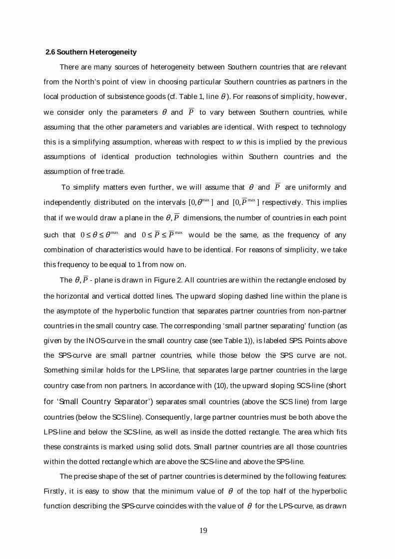
2.6 Southern Heterogeneity

There are many sources of heterogeneity between Southern countries that are relevant

from the North’s point of view in choosing particular Southern countries as partners in the

local production of subsistence goods (cf. Table 1, line θ ). For reasons of simplicity, however,

we consider only the parameters θ and P to vary between Southern countries, while

assuming that the other parameters and variables are identical. With respect to technology

this is a simplifying assumption, whereas with respect to w this is implied by the previous

assumptions of identical production technologies within Southern countries and the

assumption of free trade.

To simplify matters even further, we will assume that θ and P are uniformly and

independently distributed on the intervals [0,θmax ] and [0,P max ] respectively. This implies

that if we would draw a plane in the P,θ dimensions, the number of countries in each point

such that max0 θθ ≤≤ and max0 PP ≤≤ would be the same, as the frequency of any

combination of characteristics would have to be identical. For reasons of simplicity, we take

this frequency to be equal to 1 from now on.

The P,θ - plane is drawn in Figure 2. All countries are within the rectangle enclosed by

the horizontal and vertical dotted lines. The upward sloping dashed line within the plane is

the asymptote of the hyperbolic function that separates partner countries from non-partner

countries in the small country case. The corresponding ‘small partner separating’ function (as

given by the INOS-curve in the small country case (see Table 1)), is labeled SPS. Points above

the SPS-curve are small partner countries, while those below the SPS curve are not.

Something similar holds for the LPS-line, that separates large partner countries in the large

country case from non partners. In accordance with (10), the upward sloping SCS-line (short

for ‘Small Country Separator’) separates small countries (above the SCS line) from large

countries (below the SCS line). Consequently, large partner countries must be both above the

LPS-line and below the SCS-line, as well as inside the dotted rectangle. The area which fits

these constraints is marked using solid dots. Small partner countries are all those countries

within the dotted rectangle which are above the SCS-line and above the SPS-line.

The precise shape of the set of partner countries is determined by the following features:

Firstly, it is easy to show that the minimum value of θ of the top half of the hyperbolic

function describing the SPS-curve coincides with the value of θ for the LPS-curve, as drawn

20

in the Figure. Secondly, the SCS-curve intersects with this minimum. Third, the vertical

asymptote of the hyperbolic SPS-curve is exactly halfway point M and the origin. Finally, the

tangent of 1λ is twice as large as that of 0λ . In short, we have thatφ

λ 1)1( =tg ,

)0(2)1( λλ tgtg ⋅= , θ(M) =2 g + h ⋅ wN( )

w ⋅ φ 2 ,ϕ⋅⋅+

=w

whgNPN

)( and )(2)( NPMP ⋅= , where

we have used the notation )(Xθ to denote the θ -coordinate of a point labeled X in Figure 2,

while )(XP denotes the P -coordinate of such a point X.

Figure 2. Northern subsistence goods production partners

It is instructive to see what happens if in this setting the Northern wage goes up. In that

case the LPS-curve shifts upward and the hyperbolic SPS-curve shifts to the right,

compressing the set of partner countries into the top-right corner of the dotted rectangle. The

same happens for increases in h . Higher wages for high-skilled workers make for a smaller

number of Southern countries eligible for subsistence goods production partnerships. A rise

in the Southern wage, on the other hand, shifts down the LPS-curve, while moving points M

and N to the left. In addition, the SCS-curve gets flatter, and so does the upward-sloping

maxP

maxθ

N

MLPS

SPS

SCS

θ

P

0λ 1λ

21

asymptote of the SPS-curve, leading to an expansion of the set of partner countries in the

direction of the bottom-left corner of the dotted rectangle. A change in φ , i.e. the productivity

difference between Northern and Southern subsistence goods production technologies, will

have qualitatively similar effects as a change in the Southern wage. Interestingly, both

‘technological backwardness’ and a relatively high wage-income in the South, make for

potentially profitable partnerships between the North and the South.

We conclude that changes in Northern and Southern wages will change the set of

partner countries. The changes in this set will in turn have immediate consequences for the

demand for labour within Southern and Northern countries, and hence, for a given supply of

labour, for wages again. In order to see, therefore, how innovation, imitation and Southern

heterogeneity interact, we will now turn to a description of the associated demand for labour.

To this end, we must first cover the entry decisions of Northern firms in the Southern

subsistence goods markets.

2.7 Northern Entry of Southern Subsistence Goods Markets

Contrary to Krugman’s model, our set-up implies that Northern high-skilled workers

have two competing uses; they can produce varieties of ‘new’ luxury goods in the North, but

they can also engage in the management of subsistence goods production in the South. Given

the limited supply of Northern high-skilled labour, Southern subsistence goods production

by Northern firms therefore has an opportunity cost in the form of potential profits on

Northern luxury good production foregone.

In order to derive the optimal allocation of Northern high-skilled labour over these two

activities we define the profit function for a Northern producer, who we assume is a

monopolist both in the production of luxury goods in the North and in subsistence goods

production in the South. Thus we have for total profits iψ for the Northern producer of

variety i, and for a given Northern wage Nw , that:

∫+⋅−=max

).()(g

g

ni

Nnii

i

dvvvncwpψ (12)

22

In equation (12), nic is the level of production of the i-th Northern luxury good variety.

As we assume that it takes one unit of high-skilled labor to produce one unit of the variety, it

also represents the level of employment necessary for the production of the i-th variety. The

demand for this variety is given by equation (3). Furthermore, n(v) is the number of Southern

countries with a net operating surplus exactly equal to v, while ig is the smallest value of the

net operating surplus on subsistence goods production in some country that the i-th

Northern luxury good variety producer would want to engage in. maxg is the value of the

INOS-curve through the point ),( maxmax Pθ in Figure 2. Consequently, ∫max

).(g

g i

dvvvn represents

total profits from subsistence goods production by this Northern producer of variety i,

therefore. The control variables for a Northern variety producer are nip and ig . Recalling that

the demand for the i-th Northern luxury goods variety has a constant price elasticity of

demand equal to σ (cf. equation (3)), we find that maximisation of (12) w.r.t. the control

variables then results in the following FOC’s:

)1/(0)(// −⋅=⇒=−⋅∂∂+=∂∂ σσψ Nni

Nni

ni

ni

ni

ni wpwppccp (13.A)

00)(/ =⇒=⋅−=∂∂ iiiii gggngψ (13.B)

Equation (13.A) is the well-known Amoroso-Robinson pricing condition.7 It is also

consistent with the idea that the marginal profits at that price are equal to zero. Hence,

equations (13.A) and (13.B) taken together imply that, for given Northern wages, i.e. given

marginal costs, the scarce high-skilled labor resource should be distributed over Northern

luxury goods production and Southern partner country management in such a way that the

marginal profits in both cases are the same (and equal to zero).

Since all Northern luxury goods producers face the same marginal costs, they would set

the same price and would want to enter the same Southern markets. To simplify matters, we

will now assume that Northern producers divide markets among them rather than

7 Note that also in the case where this Northern producer would hold the monopoly over a portfolio ofproducts, (13.A)would describe the profit maximizing price for all products in that portfolio.See alsofootnote 9.

23

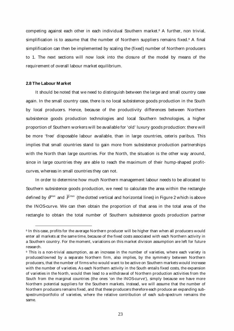
competing against each other in each individual Southern market.8 A further, non trivial,

simplification is to assume that the number of Northern suppliers remains fixed.9 A final

simplification can then be implemented by scaling the (fixed) number of Northern producers

to 1. The next sections will now look into the closure of the model by means of the

requirement of overall labour market equilibrium.

2.8 The Labour Market

It should be noted that we need to distinguish between the large and small country case

again. In the small country case, there is no local subsistence goods production in the South

by local producers. Hence, because of the productivity differences between Northern

subsistence goods production technologies and local Southern technologies, a higher

proportion of Southern workers will be available for ‘old’ luxury goods production: there will

be more ‘free’ disposable labour available, than in large countries, ceteris paribus. This

implies that small countries stand to gain more from subsistence production partnerships

with the North than large countries. For the North, the situation is the other way around,

since in large countries they are able to reach the maximum of their hump-shaped profit-

curves, whereas in small countries they can not.

In order to determine how much Northern management labour needs to be allocated to

Southern subsistence goods production, we need to calculate the area within the rectangle

defined by θ max and P max (the dotted vertical and horizontal lines) in Figure 2 which is above

the INOS-curve. We can then obtain the proportion of that area in the total area of the

rectangle to obtain the total number of Southern subsistence goods production partner

8 In this case, profits for the average Northern producer will be higher than when all producers wouldenter all markets at the same time, because of the fixed costs associated with each Northern activity ina Southern country. For the moment, variations on this market division assumption are left for futureresearch.9 This is a non-trivial assumption, as an increase in the number of varieties, where each variety isproduced/owned by a separate Northern firm, also implies, by the symmetry between Northernproducers, that the number of firms who would want to be active on Southern markets would increasewith the number of varieties. As each Northern activity in the South entails fixed costs, the expansionof varieties in the North, would then lead to a withdrawal of Northern production activities from theSouth from the marginal countries (the ones ‘on the INOS-curve’), simply because we have moreNorthern potential suppliers for the Southern markets. Instead, we will assume that the number ofNorthern producers remains fixed, and that these producers therefore each produce an expanding sub-spectrum/portfolio of varieties, where the relative contribution of each sub-spectrum remains thesame.

24

countries. The total number of management workers is then of course equal to h times the

number of Southern partner countries.

In order to calculate the relative area enclosed by the marginal INOS-curve, we need to

distinguish between five different situations which can occur in the model, as sketched in

Figure 3. The dotted rectangle corresponds to the one present in Figure 2. The horizontal

solid line is the LPS-curve from Figure 2, while the convex downward sloping curve that

joins the solid horizontal line is the downward sloping part of the SPS-curve from Figure 2.

The line emanating from the origin is the SCS line. Situations II and III differ in the point at

which the SCS line intersects with the vertical dotted line. In Situation II the SCS line leaves

the box at the top while in Situation III the SCS-line is flatter and therefore intersects the

vertical boundary of the box.

Figure 3. Possible INOS-curve constellations

Note that in cases I and V, there won’t be any eligible Southern subsistence goods

production partners, since partner countries must always be above the solid line and above

the SPS curve, as well as within the dotted rectangle. This implies that only the areas of the

North-East corners of the rectangles in as far as they are above the SPS-curve and the LPS-

curve are indeed partner countries. So, in order to calculate total management labour

demand, we need to be able to identify the five different cases.

Let Q be the (virtual) point of intersection of the convex SPS-curve with the horizontal

dotted curve. Further, let M be the point where the convex curve joins the solid horizontal (cf.

Figure 2 again) and let T be the point of intersection of the SCS curve with the horizontal line

at θ max . Case I will now obviously be identifiable by the requirement that the horizontal LPS-

curve lies above maxθ . In order to identify case V, we must have max)( PQP ≥ . For case IV

M

P

θ

Case I

Q

M

P

θ

Case IV

Q

M

P

θ

Case V

R

TQ

M

P

θ

Case II

TZQ

M

P

θ

Case III

25

point M must be to the right of the dotted vertical and point Q must be to the left of that

vertical, i.e. max)( PQP < and P (M) ≥ P max . Cases II and III share the requirements that

max)( PQP < and P (M) < P max and differ only in the value of P (T) . For Case II we require

that P (T) < P max , while P (T) ≥ P max holds in Case III.10

In order to see how exactly the supply of low-skilled labour for old luxury goods

production can be determined, one is referred to the appendix, which highlights the

principles involved in more detail than above. The appendix also shows how the number of

partner countries and hence the distribution of high-skilled labour over its two uses can be

determined. Finally, the appendix shows how aggregate Northern profits from subsistence

goods production can be obtained.

2.9 Model Closure

In principle, the model is now fully specified, except for the choice of the numeraire,

which we take to be the Southern wage. The Northern wage can then be determined by

requiring equilibrium on the labor market.

The Northern wage can be calculated by considering that the demand for labor in the

South for its different uses can be determined, for a given Northern wage, as the latter, in

combination with the model-parameters defines the various separation curves, and hence the

actual case of the five cases mentioned above that will apply for that given wage rate.

Whether a country is a small or a large partner or no partner at all, is directly relevant,

because in the no partner case, all subsistence goods need to be produced using local

technologies. In the large partner case, only a part of the population needs to produce

subsistence goods using local technologies, while in the small country case, subsistence goods

are produced using the Northern technology only. This has immediate consequences for the

level of supply of old luxury goods in those countries. However, the use of Northern

production technologies in the South also determines how much of the total supply of

Northern labor will be available for the production of Northern luxury goods in the North.

10 We can infer from the last row in Table 1, what these identification requirements imply for theparameter and variable constellations (particularly with regard to Northern and Southern wages) ofour model.

26

For, a rise in Northern wages, for example, will make for a decrease in the number of

Southern partner countries, and hence for a higher level of Northern luxury goods supply.

Generally speaking, old luxury goods supply, but also subsistence goods supply using

either local or Northern technologies for the South taken as a whole, can be obtained by

means of direct integration over these concepts, taking the division of the South into large-,

small- and no partner countries into account, as described for the 5 cases above. Looking at

these cases more closely, we find that a lower Northern (relative) wage would move the LPS-

curve down, whereas the vertical asymptote through point N in Figure 2 would move to the

left, creating more Southern partners in the process, giving rise to a larger relative supply of

Southern luxury goods (and consequently a lower relative supply of Northern luxury goods),

ceteris paribus. Given the mark-up pricing relevant in case of luxury goods, a lower Northern

relative wage would also lower Northern relative prices, and hence increase the relative

demand for Northern luxury goods again. We thus have a relative demand curve for

Northern goods (and high-skilled production labor) that is downward-sloping in relative

Northern wages, and a Northern relative supply curve of Northern luxury goods (and high-

skilled production labor) that is upward-sloping in relative Northern wages. The equilibrium

wage rate is then defined as the point of intersection of the relative labor demand and supply

curves.

3 Some Simulation Experiments

3.1 The Base Run

The only true state variables in the model are the number of old and new luxury goods,

which change over time due to innovation and imitation. Changes in the relative sizes of

these state variables drive the rest of the model, as in the original Krugman model. For

example, a rise in the ratio B/A, increases the relative importance of old luxury goods in the

generation of utility. For a given supply of Southern labor, this will decrease the supply per

old luxury good variety and hence raise the price level of old luxury goods relative to new

luxury goods. If the B/A ratio does not change, the relative scarcity of new versus old luxury

goods remains unchanged as well, and so relative prices remain the same, as will the other

model variables. This implies that the most interesting plots we may obtain using the model,

are those coming from experiments that change the scarcity of luxury products, either

27

through changes in the rate of innovation µ (or the rate of imitation κ ) or through changes

in the direct contribution of individual luxury goods to utility (changes in )γ . For the other

experiments we have in mind, we will only present the percentage (point) deviations from

the base-run, which are constant in the absence of transitional dynamics as indicated above.

In order to obtain the base run, we have used the parameter values given in Table 2.

Several things should be noted about this particular constellation. Firstly, the Northern

production technology for subsistence goods is more efficient by a factor of three compared

to the decentralized mode of production used in the South. Secondly, the Southern

population is larger than that of the North (1.5 as opposed to 1). Third, the demand for luxury

goods is fairly price-elastic. Fourth, the North is a very productive innovator, while the South

performs less well in imitating, in relative terms at least. Because of this, the North produces

a much wider relative spectrum of luxury goods in equilibrium than the South

( 5/4)/(1/)( =+−=− µκκABA ).11

Table 2. Base Run Parameter Values

3.2 Experimental Outcomes

To illustrate the working of the model and the evolution of the variables of interest over

time, we will first solve the model numerically for a baseline combination of parameters. We

11 See section 2.2. It should be noted that the experimental outcomes in the following section areobtained for initial values of the state variables that are consistent with their steady state ratio. Fromsection 2.2, it follows immediately that the steady state ratio of the number of luxury productsproduced by the North and the number of luxury products produced by the South is equal to the ratioof the rate of innovation µ and the rate of imitation κ . With a value of B0=1, we have therefore set

5/)( 0000 ==>⋅=− AABA κµ .

Parameter Value Parameter Value Parameter Value

θ max 3 v S 0.75 κ 0.025

P max 1 vN 0.25 µ 0.1

w 1 P North 1 A0 5

h 0.05 σ 4 B0 1

28

will then run some additional simulations for a period of 10 ‘years’ in a row, for several

alternative parameterizations and compare the results to the base run. The various

experiments are listed in Table 3.

Exp. Nr. Description Parameter Base Value Exp. Value

1 Productivity Southern subs. techn. +10% Sv 0.75 0.675

2 Productivity Northern subs. techn. +10% Nv 0.25 0.225

3 Rate of innovation + 10 % µ 0.1 0.11

4 Rate of imitation + 10 % κ 0.025 0.0275

5 Southern Population +10% maxP 1.0 1.1

6 Northern Population +10% NorthP 1.0 1.17 Decreasing Returns to Variety γ 0.00 0.01

Table 3. Partial Parameter Changes by Experiment

The outcomes of the experiments are listed in Table 4, except for the ones that influence

the state variables directly (Experiments 3 & 4) and the one that influences the valuation of

variety in the decreasing returns to variety experiment (Experiment 6). For these experiments,

we will show the deviations with respect to the base run in the form of a number of plots. For

the other experiments, those same deviations are listed in Table 4.

The Table and the plots show 16 variables, see the first column of Table 4, by means of

which we sketch the events taking place. Variables 1-3 are the Southern employment shares

in local subsistence goods production, Northern subsistence goods production and ‘old’

luxury goods production. Variable 4 denotes the absolute number of Southern partner

countries, while variables 5-7 are the absolute figures for Northern profits from basic goods

production and from new luxury goods production, as well as total profits for the North.

Variable 8 denotes the share of basic goods profits for the North in total Northern profits,

while variable 9 denotes the profit share of the North in Northern free disposable income.

Variable 10 measures the ratio of free disposable income in the North and in the South (as

stated before, free disposable income in the South equals gross income less expenditures on

subsistence goods). Variable 11 provides the terms of trade, i.e. the price ratio of Northern

and Southern luxury goods. Variables 12 and 13 measures the utility that the North and the

29

South derive from consuming both old and new luxury goods, while variable 14 measures

the ratio of Northern and Southern utility. It should be noted that, because of the linear

homogeneity of the utility function in consumption levels, the utility ratio is exactly equal to

the free disposable income ratio. Finally, variables 15 and 16 measure the total number of

luxury good varieties and the share of new goods in that total, respectively.

The plots in Figures 4.A-6.B cover the same variables in the same order. The first 8 plots

per experiment cover the first 8 variables from Table 4, and the second batch of 8 plots per

experiment cover variables 9-16. 12

Variable BaseRun Exp. 1 Exp. 2 Exp. 5 Exp. 6

1 Psubsloc/PS (%) 14.60 +5.70 -1.20 +0.50 -0.41

2 PsubsN/PS (%) 40.09 -4.23 -1.11 +0.89 +0.24

3 PluxS/PS (%) 45.31 -1.48 +2.32 -1.40 +0.16

4 Npartners 2.30 -8.66 +1.86 +9.86 +0.76

5 profitsNbas 0.24 -33.28 +11.04 +14.47 +1.25

6 profitsNlux 0.30 +1.59 +0.83 +3.19 +8.32

7 profitsNtot 0.54 -14.05 +5.41 +8.25 +5.15

8 profitsNbas/profitsNtot (%)

44.85 -10.035 +2.40 +2.58 -1.66

9 profitsNtot/fdispincN (%)

34.84 -3.45 +0.96 +0.80 -0.43

10 fdispincN/fdispincS

4.14 -26.61 +2.59 -12.54 +6.45

11 ToT (pN/pS) 1.35 +0.46 +1.08 +4.53 -2.59

12 UN 2.14-2.76 -4.86 +1.91 +3.03 +8.22

13 US 0.52-0.68 +29.63 -0.66 +17.81 +1.66

14 UN/US 4.14 -26.61 +2.59 -12.54 +6.45

15 A 5.00-11.79 0.00 0.00 0.00 0.00

16 (A-B)/A (%) 80.00 0.00 0.00 0.00 0.00

Table 4. Outcomes by Experiment: % Differences between Steady States

12 Plots are shown from left to right continuing on the next line of plots.

30

Results Base Run

The base run results indicate that, for the base run parameterization, subsistence goods

production is an important source of profits for the North. In addition, it is an important

source of employment for the South. It should be noted that there are 2.3 partners in this case,

which is actually larger than the total population of the South. This is because the average

population size of a country equals 0.5, since we have assumed that the density of Southern

countries in each point within the dotted rectangle in Figure 2 equals 1. Hence, the number of

Southern countries is necessarily larger than the Southern population. Because the North

produces a much wider spectrum of luxuries than the South, its free disposable income is

much larger than in the South, also because profits amount to about one third of free

disposable income in the North. The terms of trade are very favorable for the North, and so is

the distribution of utility between the North and the South. Note that in the 10 ‘year’

simulation period, the total number of luxury goods more than doubles. However, the share

of Northern luxury goods in total luxury goods remains constant at 80 percent.

Results Experiment 1: a 10% productivity rise in local subsistence goods productivity

Such a productivity rise lowers Southern prices for subsistence goods q, and therefore

also lowers prices for the basic goods produced by the North. The marginal Southern

countries now yield lower profit, turning them in fact extra-marginal. Consequently the

number of Southern partner countries is reduced by almost 9 percent. This forces those

Southern countries to move their subsistence production labor from Northern subsistence

production technologies into local subsistence technologies, which leads therefore to a fall in

subsistence labour productivity on that account (Northern technology still outperforms the

improved Southern subsistence technology). However, as the local subsistence technology

itself has increased in productivity, the overall productivity effect is positive, leading to more

Southern labor resources being available for luxury goods production, and hence to a (slight)

fall in the terms of trade for the South. Nonetheless, the overall effect on Southern utility is

very positive, because free disposable income for the South rises significantly.13

13 It should be noted that because we have aggregated over partner countries, some of the differentialcountry results go unnoticed. For example, if an extra-marginal Southern country would become apartner country, the real income effect of such a change would be much bigger for a small country than

31

Results Experiment 2: a 10% productivity rise in Northern subsistence goods productivity

The results for this experiment. experiment, except for the change in employment in

Northern subsistence technologies. Even though the number of partner countries increases

(because the productivity increase of the Northern technology raises profits on Northern

subsistence goods production, ceteris paribus, turning some of the previously non-partner

countries into partners), the 10 % productivity increase reduces the overall labor

requirements in Northern subsistence goods production. With more partner countries and

higher Northern subsistence goods productivity, there is now ‘spare’ Southern labor that can

be used to increase the production of luxury goods. This however, leads to a deterioration of

the terms of trade for the South to such an extent that total utility actually falls for the South,

albeit only slightly. For the North, the effects are all positive.

Results Experiment 3: a 10 % increase in the rate of innovation in the North

The results of this experiment are shown in Figures 4.A and 4.B below. The results are

very much as expected, as they closely resemble the ones obtained by Krugman: a higher rate

of innovation increases the relative scarcity of Northern luxury goods per variety, and hence

raises the terms of trade, and also Northern wages. This reduces the number of Southern

partner countries, and forces the South to move labor into local subsistence production. The

effect is a lower supply of Southern luxury goods, which limits the rise in the terms of trade

for the North to some extent. Free disposable income for the South falls, but utility for the

South – perhaps somewhat surprisingly – does not. The reason is that utility per dollar spent

has risen through the love of variety effect (further called the ‘LOV-effect’), which is

associated with an expansion of the total number of luxury goods. In this case the LOV-effect

is so strong that it more than compensates the negative effects on utility of the drop in free

disposable income. The conclusion that the overall utility effect is positive both for the North

and the South therefore crucially hinges on the relative strength of the LOV-effect.

for a large country, as in the latter case part of subsistence production still uses old, relatively labourintensive, local production technology.

32

4 6 8 10Time

0.1

0.2

0.3

0.4

0.5

tot Total Profits N

4 6 8 10Time

-0.6

-0.5

-0.4

-0.3

-0.2

-0.1

100 bas tot Profits Bas Total Profits

4 6 8 10Time

-0.6

-0.4

-0.2

basN Profits N from basic goods

4 6 8 10Time

0.25

0.5

0.75

1

1.25

1.5

luxN Profits N from luxury goods

4 6 8 10Time

-0.1

-0.08

-0.06

-0.04

-0.02

Share Empl . Southern lux goods

4 6 8 10Time

-0.4

-0.3

-0.2

-0.1

Npartners Number Southern partners

4 6 8 10Time

0.05

0.1

0.15

0.2

0.25

Share Empl . local tech basics

4 6 8 10Time

-0.15

-0.125

-0.1

-0.075

-0.05

-0.025

Share Empl . Northern tech basics

Figure 4.A Experiment 3: Rate of Innovation + 10 %, Plots I-VIII

33

4 6 8 10Time

2

4

6

8

N goods Number luxury goods

4 6 8 10Time

0.2

0.4

0.6

0.8

1

Share 100 nnew nnew nold 4 6 8 10Time

0.2

0.4

0.6

0.8

1

1.2

US Utility South

4 6 8 10Time

0.2

0.4

0.6

0.8

1

1.2

UN US Utility ratio N S4 6 8 10Time

0.25

0.5

0.75

1

1.25

1.5

ToT Terms of Trade pN pS

4 6 8 10Time

0.5

1

1.5

2

2.5

UN Utility North

4 6 8 10Time

-0.2

-0.15

-0.1

-0.05

shareN IncomeShare Profits North

4 6 8 10Time

0.2

0.4

0.6

0.8

1

1.2

FDINCN S Free Disp . Inc. Ratio N S

Figure 4.B Experiment 3: Rate of Innovation + 10 %, Plots IX-XVI

34

Results Experiment 4: a 10% increase in the rate of imitation in the South

Like the increase in the rate of Northern innovation, an increase in the rate with which

the South imitates Northern luxury good varieties leads to out-of-steady state dynamics,

which drive the evolution of all variables.

Compared with the base run, the share of luxury goods produced in the South rises

somewhat over time. As the share of luxury goods produced in the South rises, the volume

produced of each of these goods falls. This, in turn, raises the relative price of old luxury

goods, which represents a terms of trade benefit for the South. With the relative price (and

therefore the profitability) of Northern varieties thus diminished, Northern labor moves from

the production of luxury goods in the North into subsistence goods production in the South.

Utility in the South therefore rises not only because of the initial change in the terms-of-trade,

but also due to an income effect associated with a more intensive use of the more efficient

Northern technology in subsistence good production.

This experiment offers a theoretical explanation for the empirically observed move of

multinationals into subsistence goods in recent years. According to the current experiment,

this move could be the endogenous response of Northern firms to increasing imitation by

Southern firms. Hence, greater involvement of the North in Southern subsistence goods

production does not necessarily arise because the benefits from entering Southern markets

have become greater over time, but because the opportunity costs in terms of luxury good

production foregone have dwindled.

Finally, it should be noted that this development is a net benefit for both North and

South. That is, the North gains despite the loss of some monopolies and the associated rents

and its terms of trade loss. The reason is the higher total volume of old luxury goods

produced, enabled by the more efficient production of subsistence goods, releases labor from

inefficient local production in the South. Because the labor thus released is used in old luxury

goods production, the negative terms of trade effects of increased imitation for the North are

mitigated to such an extent, that both the North and the South may actually gain in utility

terms, albeit only very slightly for the North and in a much more outspoken manner for the

South.

35

4 6 8 10Time

-0.5

-0.4

-0.3

-0.2

-0.1

tot Total Profits N

4 6 8 10Time

0.1

0.2

0.3

0.4

0.5

0.6100 bas tot Profits Bas Total Profits

4 6 8 10Time

0.1

0.2

0.3

0.4

0.5

0.6

0.7

basNProfits N from basic goods

4 6 8 10Time

-1.5

-1.25

-1

-0.75

-0.5

-0.25

luxN Profits N from luxury goods

4 6 8 10Time

0.02

0.04

0.06

0.08

Share Empl . Southern lux goods

4 6 8 10Time

0.1

0.2

0.3

0.4

NpartnersNumber Southern partners

4 6 8 10Time

-0.25

-0.2

-0.15

-0.1

-0.05

Share Empl . local tech basics

4 6 8 10Time

0.02

0.04

0.06

0.08

0.1

0.12

0.14

Share Empl . Northern tech basics

Figure 5.A Experiment 4: Rate of Imitation + 10 %, Plots I-VIII

36

4 6 8 10Time

-1

-0.5

0.5

1

N goods Number luxury goods

4 6 8 10Time

-1

-0.8

-0.6

-0.4

-0.2

Share 100 nnew nnew nold 4 6 8 10Time

0.2

0.4

0.6

0.8

1

1.2

US Utility South

4 6 8 10Time

-1.2

-1

-0.8

-0.6

-0.4

-0.2

UN US Utility ratio N S

4 6 8 10Time

-1.5

-1.25

-1

-0.75

-0.5

-0.25

ToT Terms of Trade pN pS

4 6 8 10Time

0.02

0.04

0.06

0.08

0.1

0.12

UN Utility North

4 6 8 10Time

0.05

0.1

0.15

0.2

shareNIncomeShare Profits North

4 6 8 10Time

-1.2

-1

-0.8

-0.6

-0.4

-0.2

FDINCN S Free Disp . Inc. Ratio N S

Figure 5.B Experiment 4: Rate of Imitation + 10 %, Plots IX-XVI

37

Results Experiment 5: a 10 % increase of the population in the South

Contrary to expectations perhaps, this has a positive effect on utility both in the North

and in the South, and more so in the South. Utility per head in the South rises by almost 8

percent (17.8 percent rise in total utility less 10 percent rise in the number of heads), even

though the terms of trade go against the South, as expected. The reason is that the number of

Southern partner countries increases by almost 10 percent. Total profits from Northern

subsistence goods production increase considerably, but the North now earns less in actual

Northern luxury goods production, leading to a fall in the free disposable income ratio for the

North and the South. However, for both the North and the South, total utility rises relative to

the base run, which is indicative of a rise in free disposable income in the North and the

South, because in this experiment there is no additional LOV-effect to take into account, as

the rates of imitation and innovation are unaffected. We conclude that an increase in the size

of the population in the South, invokes partnerships reactions by the North that increases

average labor productivity in the South, that in this case outweigh the negative terms of trade

effects for the South.

Results Experiment 6: a 10 % increase of the population in the North

A 10 percent increase in the size of the workforce in the North has negative terms of

trade effects for the North, and decreases Northern wages in the process. This creates an

incentive to move into Southern subsistence goods production and to increase the number of

partners in the South. Total profits for the North increase, but free disposable income for the

North increases by more than that, since the share of profits in free disposable income slightly

falls. In the North, utility per head falls slightly. In the South utility per head rises roughly by

as much as utility per head in the North falls. This is due to the positive terms of trade effect

for the South, but also because average labor productivity in the South has risen somewhat

due to an increased activity of the North in Southern subsistence goods production.

38

Results Experiment 7: Decreasing Returns to Variety

In this experiment we make the weight of the marginal variety in the utility function

decay with rate γ as the number of varieties increases due to innovation. Since the North

produces the latest luxury goods varieties, one can interpret this as demand becoming ever

more biased in the direction of Southern varieties, because the newest Northern varieties

contribute less and less to utility. Contrary to the other (non-innovation) experiments, one

sees that the deviations from the base-run have a tendency to grow bigger over time in

absolute terms, except for the innovation and imitation related variables, that exogenously

evolve over time. The reason is that we now have a variable, i.e. the marginal contribution to

utility of the newest luxury good, hat falls continuously over time. This will reduce the

weight of the entire spectrum of Northern luxury goods in total utility, and hence will

continuously reduce the demand for Northern varieties over time.

Comparing the Figures of experiments 3 and 7, one can immediately see that they

present qualitatively opposite results: positive deviations relative to the base run in

experiment 3 correspond with negative deviations in experiment 7, and the other way

around. This is only natural, as in experiment 3 Northern relative supply conditions per

variety became tighter due to the increase in the size of the Northern luxury goods spectrum,

whereas in experiment 7, demand per variety of the Northern goods spectrum now falls.

Consequently, Northern wages fall, and there is an incentive for the North to engage ever

more intensively in Southern subsistence goods production. Both for the North and the

South, the decreasing returns to variety results in lower utility but more so for the North as

the ratio of Northern and Southern utility falls.

39

4 6 8 10Time

-1.8

-1.6

-1.4

-1.2

tot Total Profits N

4 6 8 10Time

1.2

1.4

1.6

1.8

2

100 bas tot Profits Bas Total Profits

4 6 8 10Time

1.2

1.4

1.6

1.8

2.2

2.4

2.6

basN Profits N from basic goods

4 6 8 10Time

-5.5

-4.5

-4

-3.5

-3

-2.5

luxN Profits N from luxury goods

4 6 8 10Time

0.15

0.175

0.225

0.25

0.275

0.3

0.325

Share Empl . Southern lux goods

4 6 8 10Time

0.8

1.2

1.4

1.6

Npartners Number Southern partners

4 6 8 10Time

-0.7

-0.6

-0.5

-0.4

Share Empl . local tech basics

4 6 8 10Time

0.25

0.35

0.4

0.45

0.5

Share Empl . Northern tech basics

40

Figure 6.A Experiment 7: Decreasing Returns to Variety, Plots I-VIII

4 6 8 10Time

-1

-0.5

0.5

1

N goods Number luxury goods

4 6 8 10Time

-1

-0.5

0.5

1

Share 100 nnew nnew nold

4 6 8 10Time

-2.75

-2.5

-2.25

-1.75

-1.5

-1.25

US Utility South

4 6 8 10Time

-3.5

-3

-2.5

-2

UN US Utility ratio N S4 6 8 10

Time

-5.5

-4.5

-4

-3.5

-3

-2.5

ToT Terms of Trade pN pS

4 6 8 10Time

-6

-5

-4

-3

UN Utility North

4 6 8 10Time

0.5

0.6

0.7

0.8

shareN IncomeShare Profits North

4 6 8 10Time

-3.5

-3

-2.5

-2

FDINCN S Free Disp . Inc. Ratio N S

Figure 6.B Experiment 7: Decreasing Returns to Variety, Plots IX-XVI

41

4. Concluding Remarks

In this paper we have presented an extension of Krugman’s (1979) North-South model

by including subsistence goods production in the South next to matured luxury goods

production in the South and ‘new’ luxury goods production in the North. Subsistence goods

can be produced in the South using either a relatively efficient Northern technology that

requires a fixed amount of Northern high-skilled management input, or using less efficient

Southern local technologies. The North therefore produces subsistence goods under

increasing returns to scale. We assume that the profitability of the North in subsistence goods

production depends non-linearly on the cost of reaching the local market. We also assume

that Southern countries differ with respect to both the size of their population and the

internal connectedness of their markets. Under these circumstances, we are able to determine

which set of Southern countries would be profitable partners for the North to engage in

subsistence good production. We distinguish between small partner countries and large

partner countries. Small countries are so small that their entire population is smaller than the

size of the population that would be targeted by a profit maximizing Northern subsistence

goods supplier. Hence, in small countries marginal profit opportunities are left unused. In

large countries, all positive marginal profit opportunities are exhausted at a level of the

targeted population that is below the actual population size of the country. This implies that

it is profitable for a Northern firm to leave part of the local population un-serviced.

We have assumed that the North repatriates the rents arising from those subsistence

goods production activities from the South to the North. For the Southern partners, however,

there is a productivity effect that they can benefit from, in the sense that using the more

efficient Northern subsistence goods production techniques instead of the less efficient local

techniques, frees labor resources that can now be used to produce the tradable ‘old’ luxury

goods. Thus the South has more to trade on the world-market, but suffers a negative terms of

trade effect in the process, in combination with a positive real income effect. Whether the

overall effect on utility is positive, depends on the specific situation on hand, as we show in a

number of parameter sensitivity experiments.

Based on these experiments, we can draw a number of conclusions. The first one is that

the reactions of the model to changes in the rate of innovation work in qualitatively the same

way as in the Krugman (1979) model. A wider spectrum of Northern luxury goods, in

42

combination with the existence of latent demand for these goods, increases the scarcity of

each individual Northern variety, and presents a negative terms of trade effect for the South.

However, in this case the situation is even worse for the South, because the rise in Northern

wages that this entails, makes it less worthwhile for the North to engage in subsistence goods

production in the marginal Southern partner countries (the Southern countries currently

yielding zero profits). Thus, the marginal Southern partners become extra-marginal (i.e. non-

partners effectively), and are forced to redirect part of their labour resources into relatively

inefficient subsistence goods production again. This reduces their ability to supply old

tradable luxury goods to the world-market, which represents a real negative (free disposable)

income effect. There is also a countervailing terms of trade effect, that is positive from the

point of view of the South, but the effect is not strong enough so to compensate the negative

income effect.

The second conclusion is that changes in the productivity of the North and of the South

in subsistence goods production work out favorably for the region that owns the technology

whose productivity has increased, but unfavorably for the other region. This suggests that

Northern productivity increases in subsistence goods production may not be the best way to

improve utility in the South. Obviously, if the North and the South would engage in rent-

sharing, the situation might change in favor of Northern productivity increases, but at this

stage we haven’t looked more closely into this matter yet.

The third conclusion is that increases in the rate of innovation unambiguously raise

utility for both parties. However, the number of partner countries for the North decreases,

leading to a fall in average productivity for the South, and hence to lower real free disposable

income, also because there is a negative terms of trade effect from the point of view of the

South. Nonetheless, utility for the South rises absolutely, due to the LOV-effect. This result,

even though implied by the model structure, seems somewhat hard to believe. As free

disposable income in the South is far lower than in the North, one would expect the LOV-

effect there to be potentially less important than in the North, suggesting a further extension

of the decreasing returns to variety model, by making the marginal contribution coefficient of

each variety in the utility function dependent on free disposable income per head and the

variety index, rather than on the variety index alone. Stated differently, one could imagine

that for countries with a low free disposable income per head, the contribution to utility of

43

the newest varieties are lower than for countries with a higher value of income per head. At

this stage, we must leave this for future research, however.

The fourth conclusion is that the move of Western companies into Southern subsistence

goods market may actually be regarded as a natural by-product of the successful imitation

efforts by the South. Our experiment with an increase in the rate of imitation shows that this

reduces the terms of trade for the North and consequently lowers the opportunity cost of

Northern high-skilled workers in terms of the profits on Northern luxury goods production

foregone. In these circumstances, entering Southern subsistence markets becomes a more

profitable business opportunity for the North.

The fifth conclusion is that changes in population sizes in both the North and in the

South provide an incentive for the North to intensify its subsistence goods production in the

South by seeking more Southern subsistence goods production partners. In terms of utility

per head, the South would actually benefit from having a higher population, as that raises the

incentive for the North to increase the number of subsistence production partners in the

South and raise aggregate Southern productivity in the process. By contrast, a rise in the

Northern population leads to a slightly lower rise in Northern utility, and hence to a slight

fall in utility per head. Conversely, a fall in the size of the Northern population would raise

utility per head.

The sixth conclusion is that the satiation of demand for the newest luxury goods, as we

have modeled in experiment 6, leads to a continuously falling terms of trade for the North,

and an increasing incentive for the North to move into Southern subsistence goods

production. This has positive real productivity effects for the South, which, furthermore, is

accompanied by a positive terms of trade effects for the South.

44

Appendix A. Aggregation over Southern Countries

This appendix describes the outcomes of various aggregations over groups of Southern

countries. These aggregations are necessary in order to be able to determine:

1. the total demand for high-skilled labor associated with subsistence goods

production in Southern countries;

2. the demand for low-skilled labor associated with subsistence goods production in

Southern countries;

3. the profit flows associated with subsistence goods production in Southern countries.

In order to be able to do this, the distinction between large and small countries is

important again. For small countries, the population size determines the size of the profitable

subsistence market for Northern firms, whereas this is not the case for large countries. The

same applies therefore to the demand for labor in as far as it is associated with subsistence

goods production. This holds both for high-skilled management labor, as well as low-skilled

production labor. Finally, the net operating surplus depends on the combination of

characteristics of a country. Hence, aggregation over all profits earned by Northern firms in

Southern subsistence markets allows us to obtain the income flows as they arise out of

subsistence goods production.

In order to be able to perform the aggregations mentioned above, it is helpful to present

the three situations that can arise in the model for which the set of partner countries is non-

empty again (see Figure 3 in the main text):

PPP

TQ

M

θ

TQ

M

Q

M

θ

R

Situation II Situation III Situation IV

ZU V W

θ

45

We summarize the requirements for each situation in the table below:

P(Q) P(M) P(T)

Situation II P(Q) < P max P (M) < P max P (T) < P

Situation III P(Q) < P max P (M) < P max

Situation IV P(Q) < P max P (M) ≥ P max

Recalling that the vertical dotted line and the horizontal dotted line are defined bymaxPP = and maxθθ = , respectively, the number of Southern countries in which Northern

firms are engaged in subsistence production can be obtained as follows. For situation 2, draw

a horizontal line somewhere between points Q and M. This line will intersect with the convex

curve connecting points Q and M at a point further called U, as well as the straight line

connecting points M and T at a point further called V but also the vertical dotted line at a

point further called W. Obviously, the length of the line-segment connecting points U and V,

further called UV, depends on the vertical position of that line-segment, i.e. on θ . Hence, the

area associated with the small partner countries is the integral over all line-segments UV with

a θ in the interval )()..( QM θθ . Thus, for the number of small Southern partner countries in

situation II, we would find that:

∫ ∫=)(

)(

))((

))((

1Q

M

VP

UP

S dPdPθ

θ

θ

θ

θ (A.1)

where 1 is the frequency of Southern countries in each point of the area enclosed by the

vertical and horizontal dotted lines, as before. For the number of large partner countries, we

would find analogously:

∫ ∫=)(

)(

))((

))((

1Q

M

WP

VP

L dPdPθ

θ

θ

θ

θ (A.2)

46

Note that for situations III and IV, a similar procedure can be followed, but the

integration boundaries need to be adjusted somewhat. This is straightforward and therefore

not shown here.

As regards the supply of labour available for matured luxury goods production, we

need to distinguish again between large and small countries. For a small country, for

example, and using the assumption that vS<1, we must have that the total amount of low-

skilled labour not used in subsistence goods production is equal to:

P NS = P − vN ⋅ P *−v S ⋅ (P − P*) = P ⋅ (1− v S ) + (v S − vN ) ⋅ P * (A.3)

Equation (A.3) has several interesting features. First, if vS>vN as we assume, then

Northern subsistence goods production in a Southern country does indeed free resources that

become available for matured luxury goods production. Secondly, the larger the Northern

subsistence goods market P*, the more resources will be freed. Finally, lowering v S will help

free resources only in case the Southern country is big, since for small countries we have that

P* = P if 1<Sv , as we have assumed it to be the case and (A.3) reduces to:

)1( NNS vPP −⋅= (A.4)

Equation (A.4) reflects the notion that all subsistence goods production in a small

Southern country is taken over by Northern producers, by the definition of a small country.

Hence, in situation 2, we would find that the total supply of low-skilled labour in small

Southern countries, i.e. LS, that is available for matured luxury good production must in that

case be given by:

∫ ∫ −⋅=)(

)(

))((

))((

)1(Q

M

VP

UP

NS dPdvPLθ

θ

θ

θ

θ (A.5)

For a large country, (A.4) does not hold. Instead, we would have to substitute the

definition of S* from Table 1 into (A.3) , in which case we would find for low-skilled labour

supply in large Southern countries, i.e. LL , that:

47

∫ ∫ ⋅⋅−+−⋅=)(

)(

))((

))((

})()1({Q

M

WP

VP

NSSL dPdvvvPLθ

θ

θ

θ

θφθ (A.6)

Finally, total profits from subsistence goods production can be obtained as follows. The

net operating surplus per active firm in each country will be given by equation (8), where one

should realize that the net operating surplus, i.e. g , is a function of θ for large countries and

of θ and P for small countries, as apparent from Table 1. Thus we get for total profits

obtained from subsistence goods production in small Southern countries, i.e. SΠ :

∫ ∫ ⋅−⋅⋅

−⋅⋅=Π)(

)(

))((

))((

2

}2

{Q

M

VP

UP

NS dPdhwwPwPθ

θ

θ

θ

θθ

φ (A.7)

For large Southern countries we obtain, by analogy:

∫ ∫ ⋅−⋅⋅⋅=Π)(

)(

))((

))((

2 }21{

Q

M

WP

VP

NL dPdhwwθ

θ

θ

θ

θθφ (A.8)

Using the principles outlined above, we first have to obtain the expressions for the

points U,V and W, before we can actually evaluate all the integrals. Since these expressions

are relatively complicated for the small country case, the integrals themselves become

relatively unintelligible. Hence we do not report them here. For the simulations we have

performed, we have evaluated these integrals numerically as part of the numerical simulation

of the entire model, using the Mathematica programming package.

48

References

Chui, M., Levine, P., Mansoob Musrshed, S. and Pearlman, J. (2002), North-South Models of

Growth and Trade, Journal of Economic Surveys, Vol. 16, No. 2, pp. 123-165.

Grossman, G. M. and Helpman, E. (1991). Quality ladders and product cycles. The Quarterly

Journal of Economics, pages 557–586.

Helpman, E. (1993), Innovation, imitation and intellectual property rights, Econometrica, 61(6):

1247-1280.

Krugman, P. (1979). A Model of Innovation, Technology Transfer, and the World Distribution

of Income. The Journal of Political Economy, 87(2):253-266.

Matsuyama, K. (2000), A Ricardian Model with a Continuum of Goods under Nonhomothetic

Preferences: Demand Complementarities, Income Distribution and North-South Trade,

Journal of Political Economy, 108(6):1093-1120.

Prahalad, C.K, and Hammond, A. (2002), Serving the World’s Poor, Profitably, Harvard

Business Review, September 2002, pp.4-11.

Prahalad, C.K. (2006), The Fortune at the Bottom of the Pyramid: Eradicating Poverty through

Profits, Wharton School Publishing.

Romer, P. M. (1990). Endogenous technological change. The Journal of Political Economy,

98(5):S71–S102.

49

The UNU-MERIT WORKING Paper Series

2008-01 Science, Technology and Development: Emerging concepts and visions by Luc Soete

2008-02 Reframing technical change: Livestock Fodder Scarcity Revisited as InnovationCapacity Scarcity. Part 1. A Review of Historical and Recent Experiences by AndyHall, Rasheed Sulaiman V., Mona Dhamankar, Peter Bezkorowajnyj & Leela Prasad

2008-03 Reframing technical change: Livestock Fodder Scarcity Revisited as InnovationCapacity Scarcity. Part 2. A Framework for Analysis by Andy Hall, Rasheed Sulaiman,V. and Peter Bezkorowajnyj

2008-04 Reframing technical change: Livestock Fodder Scarcity Revisited as InnovationCapacity Scarcity.Part 3. Tools for Diagnosis and Institutional Change in InnovationSystems by Andy Hall, Rasheed Sulaiman and Peter Bezkorowajnyj

2008-05 Is Inter-Firm Labor Mobility a Channel of Knowledge Spillovers? Evidence from aLinked Employer-Employee Panel by Mika Maliranta, Pierre Mohnen & Petri Rouvinen

2008-06 Financial Constraints and Other Obstacles:Are they a Threat to Innovation Activity?By P. Mohnen, F.C. Palm, S. Schim van der Loeff and A. Tiwari

2008-07 Knowledge-based productivity in ‘low-tech’ industries: evidence from firms indeveloping countries by Micheline Goedhuys, Norbert Janz and Pierre Mohnen

2008-08 The Voyage of the Beagle in Innovation Systems Land.Explorations on Sectors,Innovation, Heterogeneity and Selection by Martin Srholec & Bart Verspagen

2008-09 Crafting Firm Competencies to Improve Innovative Performance by Boris Lokshin,Anita van Gils & Eva Bauer

2008-10 The Economics and Psychology of Personality Traits by Lex Borghans, Angela LeeDuckworth, James J. Heckman & Bas ter Weel

2008-11 Embedding Research in Society: Development Assistance Options for SupportingAgricultural Innovation in a Global Knowledge Economy by Andy Hall

2008-12 Playing in Invisible Markets: Innovations in the Market for Toilets to Harness theEconomic Power of the Poor by Shyama V. Ramani

2008-13 Explaining Success and Failure in Development by Adam Szirmai

2008-14 Running The Marathon by William Cowan, Robin Cowan and Patrick Llerena

2008-15 Productivity effects of innovation, stress and social relations by Rifka Weehuizen, BulatSanditov and Robin Cowan

2008-16 Entrepreneurship and Innovation Strategies in ICT SMEs in Enlarged Europe (EU25)by Kaushalesh Lal and Theo Dunnewijk

2008-17 Knowledge Transfers between Canadian Business Enterprises and Universities: DoesDistance Matter? By Julio M. Rosa & Pierre Mohnen

2008-18 Multinationals are Multicultural Units: Some Indications from a Cross-Cultural Studyby Nantawan Noi Kwanjai & J. Friso den Hertog

50

2008-19 The Innovativeness of Foreign Firms in China by Branka Urem, Ludovico Alcorta andTongliang An

2008-20 Beyond the emission market: Kyoto and the international expansion of wastemanagement firms by Ionara Costa, Asel Doranova and Geert-Jan Eenhoorn

2008-21 The ‘making of’ national giants: technology and governments shaping the internationalexpansion of oil companies from Brazil and China by Flavia Carvalho and AndreaGoldstein

2008-22 If the Alliance Fits . . . : Innovation and Network Dynamics by Robin Cowan & NicolasJonard

2008-23 Facing the Trial of Internationalizing Clinical Trials to Developing Countries: WithSome Evidence from Mexico by Fernando Santiago-Rodriguez

2008-24 Serving low-income markets: Rethinking Multinational Corporations’ Strategies byShuan SadreGhazi and Geert Duysters

2008-25 A percolation model of eco-innovation diffusion: the relationship between diffusion,learning economies and subsidies by Simona Cantono and Gerald Silverberg

2008-26 New Europe’s Promise for Life Sciences by Sergey Filippov and Kálmán Kalotay

2008-27 A closer look at the relationship between life expectancy and economic growth byThéophile T. Azomahou, Raouf Boucekkine, Bity Diene

2008-28 Regional Capital Inputs in Chinese Industry and Manufacturing, 1978-2003 by LiliWang & Adam Szirmai

2008-29 Worker remittances and government behaviour in the receiving countries by ThomasZiesemer

2008-30 Strategic motivations for Sino-Western alliances: a comparative analysis of Chineseand Western alliance formation drivers by Tina Saebi & Qinqin Dong

2008-31 Changing Configuration of Alternative Energy Systems by Radhika Bhuyan and LynnMytelka

2008-32 Promoting clean technologies: The energy market structure crucially matters byThéophile T. Azomahou, Raouf Boucekkine, Phu Nguyen-Van

2008-33 Local Knowledge Spillovers, Innovation and Economic Performance in DevelopingCountries: A discussion of alternative specifications by Effie Kesidou and AdamSzirmai

2008-34 Wage effects of R&D tax incentives: Evidence from the Netherlands by Boris Lokshinand Pierre Mohnen

2008-35 Cross-border Investment and Economic Integration: The Case of Guangdong Provinceand Hong Kong SAR by Naubahar Shari and Can Huang

2008-36 Radical versus non-radical inventions by Wilfred Schoenmakers, Geert Duysters &Wim Vanhaverbeke

51

2008-37 Localized Innovation, Localized Diffusion and the Environment: An Analysis of CO2Emission Reductions by Passenger Cars, 2000-2007 by Bart Los and Bart Verspagen

2008-38 The economic impact of AIDS in sub-Saharan Africa by Théophile T. Azomahou, RaoufBoucekkine, Bity Diene

2008-39 Further results on bias in dynamic unbalanced panel data models with an application tofirm R&D investment by Boris Lokshin

2008-40 A multilevel analysis of innovation in developing countries by Martin Srholec

2008-41 Experimentation with strategy and the evolution of dynamic capability in the IndianPharmaceutical Sector by Suma Athreye, Dinar Kale & Shyama V. Ramani

2008-42 The Impact of Social Capital on Crime: Evidence from the Netherlands by I.SemihAkcomak and Bas ter Weel

2008-43 Portrait of an Odd-Eyed Cat: Cultural Crossing as a Trademark for a Dutch-ThaiStrategic Alliance by Nantawan Noi Kwanjai & J Friso den Hertog

2008-44 The challenge of measuring innovation in emerging economies’ firms: a proposal of anew set of indicators on innovation by Luciana Manhães Marins

2008-45 Intra-firm Technology Transfer and R&D in Foreign Affiliates: Substitutes orComplements? Evidence from Japanese Multinational Firms by Rene Belderbos,Banri Ito, Ryuhei Wakasugi

2008-46 To Be or Not to Be at the BOP: A One-North-Many-Souths Model withSubsistence and Luxury Goods by Adriaan van Zon and Tobias Schmidt