working paper series 5
TRANSCRIPT

WORKING PAPER SERIES 5 8002
Kamil Dybczak, David Voňka and Nico van der Windt:The Effect of Oil Price Shocks on the Czech Economy

WORKING PAPER SERIES
The Effect of Oil Price Shocks on the Czech Economy
Kamil Dybczak David Voňka
Nico van der Windt
5/2008
CNB WORKING PAPER SERIES The Working Paper Series of the Czech National Bank (CNB) is intended to disseminate the results of the CNB’s research projects as well as the other research activities of both the staff of the CNB and collaborating outside contributor, including invited speakers. The Series aims to present original research contributions relevant to central banks. It is refereed internationally. The referee process is managed by the CNB Research Department. The working papers are circulated to stimulate discussion. The views expressed are those of the authors and do not necessarily reflect the official views of the CNB. Printed and distributed by the Czech National Bank. Available at http://www.cnb.cz. Reviewed by: Jan Hošek (Czech National Bank) Michal Kejak (CERGE-EI, Prague) Marcelo Sánchez (European Central Bank)
Project Coordinator: Kamil Galuščák © Czech National Bank, November 2008 Kamil Dybczak, David Voňka, Nico van der Windt

The Effect of Oil Price Shocks on the Czech Economy
Kamil Dybczak, David Vonka and Nico van der Windt ∗
Abstract
In the course of 2002 up to the end of 2007, very steep growth of oil prices, but noremarkable slowdown of either the world economy or the Czech economy, was observed.This phenomenon raises a question about the impact of oil prices on modern economies.Analyzing the available data we can conclude that notwithstanding the full dependence ofthe Czech economy on oil imports, its overall dependence on imported energy sources isrelatively low. Compared to the EU15 level the energy intensity of the Czech economy isquite high. Nevertheless, further improvements in this area are expected. Furthermore, theappreciation of CZK and the set-up of the tax system significantly reduced the volatilityof the consumer oil price between 2002 and 2007. Using a structural CGE model wequantify the impact of oil price changes on the Czech economy and demonstrate that it isnot dramatic despite the oil price turmoil in the years 2000 to the end of 2007. We findthat a 20% increase in the CZK oil price tends to decrease the GDP level by 1.5% and0.8% in the short and long run, respectively. Short-run annual GDP growth decreases by0.3 p.p. Concerning prices, inflation would accelerate by around 0.4 p.p. per annum inthe short run.
JEL Codes: C68, Q43.Keywords: CGE, Czech Republic, oil price.
∗ Kamil Dybczak, Czech National Bank (e-mail: [email protected]);David Vonka, Tilburg University (e-mail: [email protected]);Nico van der Windt, Erasmus University (e-mail:[email protected]).
This work was supported by Czech National Bank Research Project No. E2/2007.
The authors would like to thank Jan Hosek, Michal Kejak, Marcelo Sanchez, Kamil Galuscak, KaterinaSmıdkova and participants at the interim and final seminars at the Czech National Bank for helpful discussion andcomments. All errors and omissions are ours. The views expressed are those of the authors and do not necessarilyreflect the views of the Czech National Bank.
2 Kamil Dybczak, David Vonka and Nico van der Windt
Nontechnical Summary
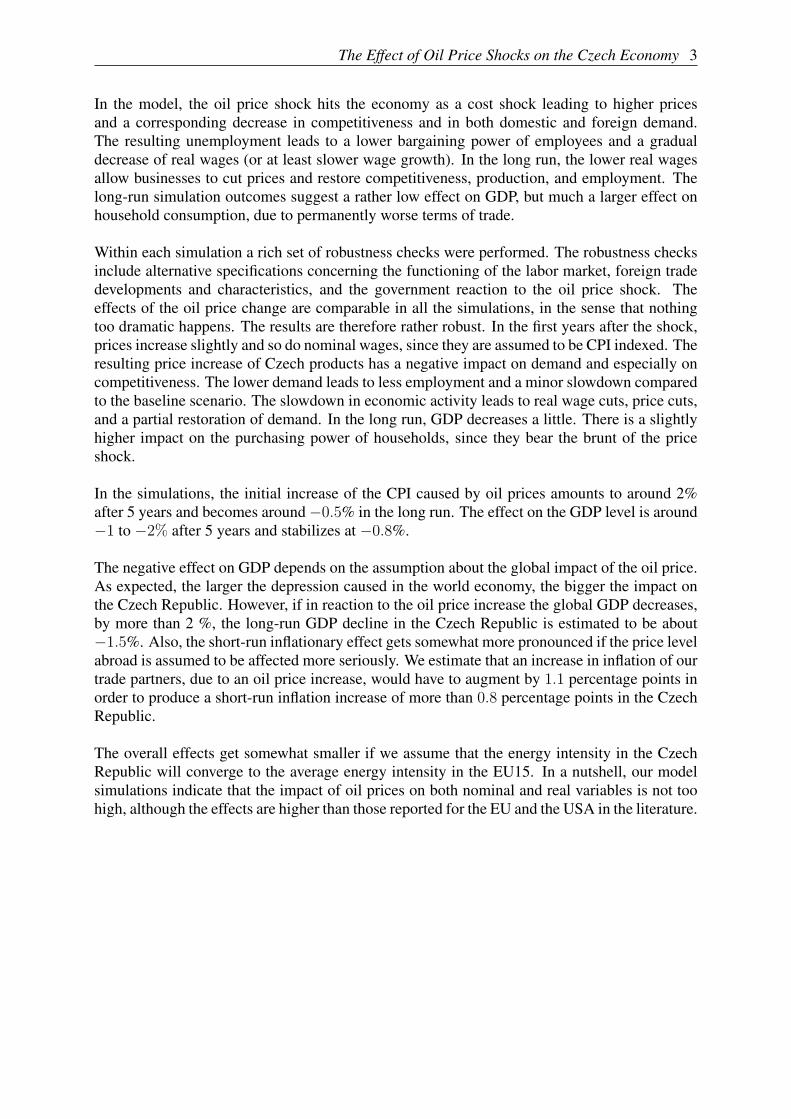
Very steep growth of oil prices was observed in the course of 2002 up to the end of 2007.As this paper was written (end 2007 – beginning 2008), the USD price of a barrel of Brentoil was threatening to reach 100 USD. By the time of submission (June 2008) it had reached140 USD. This amounts to an increase by a factor of six since the beginning of this millennium.Simultaneously, until 2007 we observed no serious slowdown in the world economy. This paperanalyzes why the impact of the oil price boom seems to have been so small. The economicproblems which came thereafter were mainly triggered by other factors. On the contrary, until2007 the world was experiencing an economic boom, mainly thanks to developments in China,India, and Russia. The Czech economy, too, was going through one of its better periods.
The Czech economy is not self-sufficient in its energy needs, but its dependence on imports ofenergy is relatively low, mainly because of domestic coal mining. This is reflected in the struc-ture of energy use, where imported oil plays a smaller role than in other countries. But like manyother post-communist countries, the Czech economy uses a relatively large amount of energyper unit of output. In other words, its so-called energy intensity is rather high. This intensityhas been decreasing in the past decade and a further decrease can reasonably be expected.
The Czech Republic imports basically all the crude oil it needs, mainly from post-Soviet coun-tries. Very little of it is used for electricity and heat production; the rest is transformed intovarious oil products that satisfy around 70% of the domestic market demand. Oil products –mainly motor gasoline and diesel – are also imported, most often from neighboring countries.The greatest part of the oil products is used in transport and in the chemical industry.
The price of oil products that a Czech firm or consumer faces is dependent not only on the USDprice of oil on the world market. An important determinant is the USD exchange rate. Theappreciation of CZK has moderated the impact of the past oil price changes greatly. Anothercushioning factor is the system of consumption taxes on gasoline and diesel, since this tax islevied per quantity (liter) and not per monetary value. Therefore, the tax does not change asthe oil price changes. During the period January 2000 – June 2008, the world oil price in USDhas risen by around 600%. Thanks to the compound effect of strong CZK appreciation and thestabilizing impact of consumption taxes, Czech consumers have faced only a 50% increase inthe price of gasoline and diesel in the same period. The dampening role of taxes exceeded thatof the exchange rate.
Regression outcomes of several domestic price indices on the oil price suggest that the effectof the oil price on aggregated price indices is very low. A 10% increase in the world oil pricecannot be expected to increase the domestic PPI or CPI by more than 0.1%.
A CGE model is used for the oil price simulations. The model incorporates (inter alia) a verydetailed industrial production structure based on input-output tables for the Czech economy.
We simulate the effect of a gradual increase of the oil price Czech consumers face (i.e., thefinal consumption price in CZK) by 5% p.a. over 4 years. The three simulations differ in theirassumptions about the potential future improvement in oil use intensity and in their assumptionsabout the effects of oil prices on Czech trade partners.
The Effect of Oil Price Shocks on the Czech Economy 3
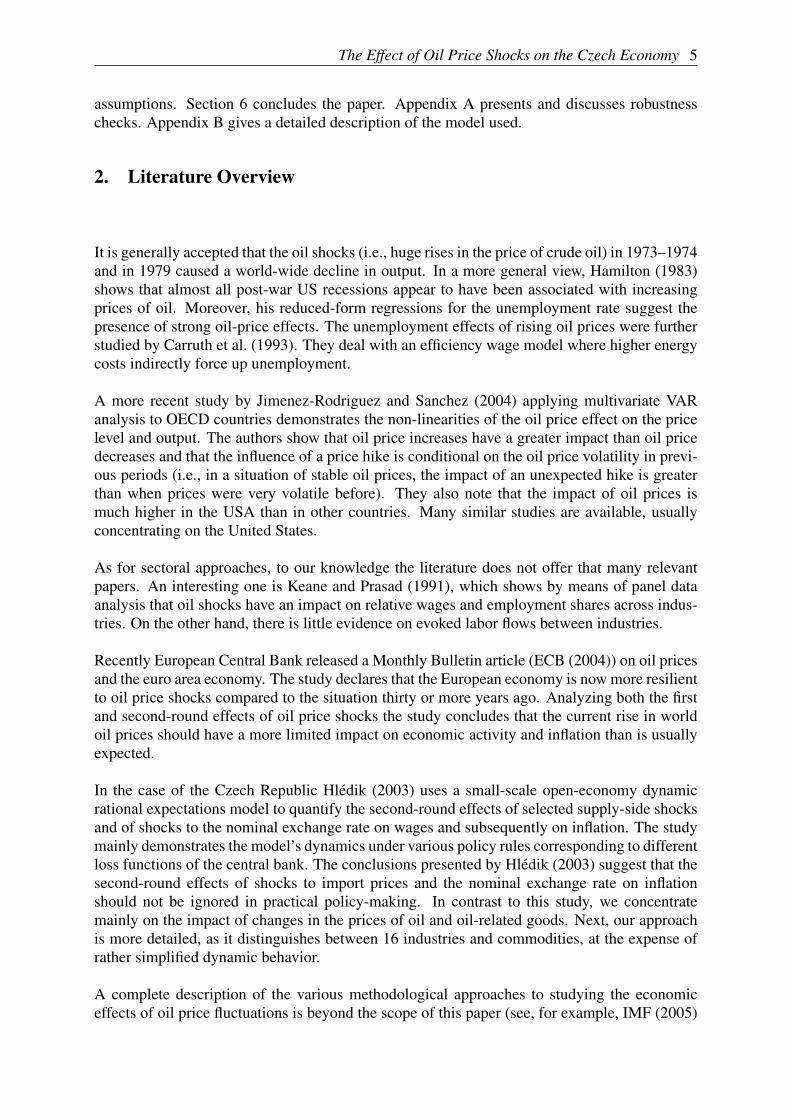
In the model, the oil price shock hits the economy as a cost shock leading to higher pricesand a corresponding decrease in competitiveness and in both domestic and foreign demand.The resulting unemployment leads to a lower bargaining power of employees and a gradualdecrease of real wages (or at least slower wage growth). In the long run, the lower real wagesallow businesses to cut prices and restore competitiveness, production, and employment. Thelong-run simulation outcomes suggest a rather low effect on GDP, but much a larger effect onhousehold consumption, due to permanently worse terms of trade.
Within each simulation a rich set of robustness checks were performed. The robustness checksinclude alternative specifications concerning the functioning of the labor market, foreign tradedevelopments and characteristics, and the government reaction to the oil price shock. Theeffects of the oil price change are comparable in all the simulations, in the sense that nothingtoo dramatic happens. The results are therefore rather robust. In the first years after the shock,prices increase slightly and so do nominal wages, since they are assumed to be CPI indexed. Theresulting price increase of Czech products has a negative impact on demand and especially oncompetitiveness. The lower demand leads to less employment and a minor slowdown comparedto the baseline scenario. The slowdown in economic activity leads to real wage cuts, price cuts,and a partial restoration of demand. In the long run, GDP decreases a little. There is a slightlyhigher impact on the purchasing power of households, since they bear the brunt of the priceshock.
In the simulations, the initial increase of the CPI caused by oil prices amounts to around 2%after 5 years and becomes around−0.5% in the long run. The effect on the GDP level is around−1 to −2% after 5 years and stabilizes at −0.8%.
The negative effect on GDP depends on the assumption about the global impact of the oil price.As expected, the larger the depression caused in the world economy, the bigger the impact onthe Czech Republic. However, if in reaction to the oil price increase the global GDP decreases,by more than 2 %, the long-run GDP decline in the Czech Republic is estimated to be about−1.5%. Also, the short-run inflationary effect gets somewhat more pronounced if the price levelabroad is assumed to be affected more seriously. We estimate that an increase in inflation of ourtrade partners, due to an oil price increase, would have to augment by 1.1 percentage points inorder to produce a short-run inflation increase of more than 0.8 percentage points in the CzechRepublic.
The overall effects get somewhat smaller if we assume that the energy intensity in the CzechRepublic will converge to the average energy intensity in the EU15. In a nutshell, our modelsimulations indicate that the impact of oil prices on both nominal and real variables is not toohigh, although the effects are higher than those reported for the EU and the USA in the literature.

4 Kamil Dybczak, David Vonka and Nico van der Windt
1. Introduction
Very steep growth of oil prices was observed in the course of 2002 up to the end of 2007. At thetime of writing this paper (end of 2007 – beginning 2008), the USD price of a barrel of Brentoil was threatening to reach 100 USD. At the time of submission of the final version (May2008) we were at 140 USD. This amounts to an increase by a factor of 6 since the beginning ofthis millennium. Simultaneously, until recently we observed no serious slowdown in the worldeconomy, and the recent slowdown is arguably due to other causes. On the contrary, the worldexperienced an economic boom, mainly thanks to developments in China, India, and Russia.The Czech economy, too, is going through one of its better periods.
How is this possible? During the oil crises in 1973 the oil price quadrupled, which led to aperiod of stagflation. The effects of the 1979 crisis were also pronounced. Has the impact of oilprices on the economy really become so small during the past 30 years?
This paper studies the impact of oil prices on the Czech economy from several perspectives.First, we analyze the available data on the sources and use of energy in the Czech Republic andthe determinants of energy prices for the domestic consumer. Second, our main tool is a com-putable general equilibrium (CGE) model of the Czech economy, which models the productionstructure in great detail. From both perspectives we find a rather moderate effect of oil prices onthe economy. We demonstrate that this result is rather robust with respect to reasonable changesin the assumptions. It is worth emphasizing that we do not analyze the factors behind world oilprice developments. The Czech Republic is a small open economy with no real impact on theworld oil price. Although there has been much public debate on oil price issues, to our knowl-edge there has been no detailed analysis of the reaction of the Czech economy to the oil price.Furthermore, even outside the Czech Republic, there are very few models analyzing the priceshock in such industrial detail.
Based on the results of our investigations we believe that the structure of the Czech economyis indeed different from the structure of the economies hit by the oil price shocks in the 1970s.The weight of less oil intensive industries has increased and the overall oil intensity of thetechnology used has decreased. There are more substitution possibilities in production. Theseconclusions may also apply to many other countries around the world.
The paper is organized as follows. Section 2 gives an overview of the relevant literature aboutCGE models and about the impact of oil prices. Section 3 describes the sources and use of oilin the Czech economy. It focuses on a description of energy dependence and intensity (section3.1), the sources and consumption of oil (section 3.2), and pricing of oil products (section 3.3).
The CGE-model-related results are concentrated in section 4 of this paper. Section 4.1 focuseson the dissemination of the oil price shock in the model. Section 4.2 introduces the modelsimulations of the impact of oil price increases and describes their construction. Sections 4.3to 4.5 describe the results of the simulations under alternative assumptions about the potentialdevelopment of the oil intensity of the Czech economy and about the reaction of the rest of theworld to the shocks. As already mentioned, the simulations demonstrate that the impact of oilprices on the Czech economy is not really dramatic, regardless of reasonable changes in the
The Effect of Oil Price Shocks on the Czech Economy 5
assumptions. Section 6 concludes the paper. Appendix A presents and discusses robustnesschecks. Appendix B gives a detailed description of the model used.
2. Literature Overview
It is generally accepted that the oil shocks (i.e., huge rises in the price of crude oil) in 1973–1974and in 1979 caused a world-wide decline in output. In a more general view, Hamilton (1983)shows that almost all post-war US recessions appear to have been associated with increasingprices of oil. Moreover, his reduced-form regressions for the unemployment rate suggest thepresence of strong oil-price effects. The unemployment effects of rising oil prices were furtherstudied by Carruth et al. (1993). They deal with an efficiency wage model where higher energycosts indirectly force up unemployment.
A more recent study by Jimenez-Rodriguez and Sanchez (2004) applying multivariate VARanalysis to OECD countries demonstrates the non-linearities of the oil price effect on the pricelevel and output. The authors show that oil price increases have a greater impact than oil pricedecreases and that the influence of a price hike is conditional on the oil price volatility in previ-ous periods (i.e., in a situation of stable oil prices, the impact of an unexpected hike is greaterthan when prices were very volatile before). They also note that the impact of oil prices ismuch higher in the USA than in other countries. Many similar studies are available, usuallyconcentrating on the United States.
As for sectoral approaches, to our knowledge the literature does not offer that many relevantpapers. An interesting one is Keane and Prasad (1991), which shows by means of panel dataanalysis that oil shocks have an impact on relative wages and employment shares across indus-tries. On the other hand, there is little evidence on evoked labor flows between industries.
Recently European Central Bank released a Monthly Bulletin article (ECB (2004)) on oil pricesand the euro area economy. The study declares that the European economy is now more resilientto oil price shocks compared to the situation thirty or more years ago. Analyzing both the firstand second-round effects of oil price shocks the study concludes that the current rise in worldoil prices should have a more limited impact on economic activity and inflation than is usuallyexpected.
In the case of the Czech Republic Hledik (2003) uses a small-scale open-economy dynamicrational expectations model to quantify the second-round effects of selected supply-side shocksand of shocks to the nominal exchange rate on wages and subsequently on inflation. The studymainly demonstrates the model’s dynamics under various policy rules corresponding to differentloss functions of the central bank. The conclusions presented by Hledik (2003) suggest that thesecond-round effects of shocks to import prices and the nominal exchange rate on inflationshould not be ignored in practical policy-making. In contrast to this study, we concentratemainly on the impact of changes in the prices of oil and oil-related goods. Next, our approachis more detailed, as it distinguishes between 16 industries and commodities, at the expense ofrather simplified dynamic behavior.
A complete description of the various methodological approaches to studying the economiceffects of oil price fluctuations is beyond the scope of this paper (see, for example, IMF (2005)

6 Kamil Dybczak, David Vonka and Nico van der Windt
or Williams (2006), for an overview). In the following text, we therefore limit ourselves to themethod chosen in this paper and intend to explain its main properties, as developed by economicresearch.
The determinants and predictors of the world oil price are not in the centre of our interest; wetreat its development as strictly exogenous. We focus on the Czech economy, which plays noreal role in world oil price determination. For a recent treatment of this topic, see, for example,DG-ECFIN (2005a), DG-ECFIN (2005b), DG-ECFIN (2005c), and DG-ECFIN (2005d) byEuropean Commission DG ECFIN.
An interesting set of answers to frequently asked questions about oil is Kingma and Suyker(2004). It discusses the role of oil in a modern economy, the power of OPEC, the role of taxes,the oil price impacts from different studies, and many other issues related to oil.
In our research, we decide to explore computable general equilibrium (CGE) models to ex-amine the economic consequences of fluctuations in oil prices. The essence of the model isto estimate how an economy might react to changes in policy, technology or other externalfactors. The intellectual origin of (neoclassical) CGE models can be traced back to the gen-eral equilibrium theory of Walras (1926) and the input-output models pioneered by Leontief(1986). The neoclassical general equilibrium approach was rigorously elaborated by Debreu(1959). Though mathematically rigorous, this work did not pretend to describe really existingeconomic systems, but rather attempted to prove the existence of a Pareto optimal equilibriumof a competitive economy under highly restricted assumptions.
Johansen (1960) was the first to try and bridge the gap between theory and reality by devel-oping the first empirical or computable general equilibrium model, applied to the Norwegianeconomy. The Cambridge Growth Project in the UK is another example of early efforts aimedat an analogous goal. It was two decades later before CGE models became used more fre-quently, primarily in the field of (optimal) taxation and trade policies in developed countries.The Australian MONASH model is a representative of this class.
Work on a CGE model for less developed countries started in the 1970s, culminating in thepioneering work of Adelman and Robinson (1977) on Korea. This work triggered a huge streamof CGE models. These models were an improvement on the rather rigid input-output modelsbased on fixed relative prices and limited scope for substitution. The CGE models, largely basedon neoclassical optimizing behavior, were able to generate endogenously determined prices andallowed for all kinds of substitution processes – between primary inputs, between intermediateprimary inputs, and between tradable and non-tradable commodities. Furthermore, the labormarket was endogenised and even different technological strata within sectors were sometimesdistinguished.
The recessions in the developed world in the 1970s and the debt crises in the less developedworld shifted the earlier focus on development strategies, poverty, and income distribution awaytowards structural adjustment and stabilization. Trade problems were increasingly consideredimportant, and it was no surprise that CGE models became an important instrument for theanalysis of trade policies.
Recently, there has been renewed interest in the type of problems which used to be studied in the1960s and 1970s. Poverty and income distribution, though never absent in applied work, haveregained a central position, alongside environmental problems. CGE models may also become

The Effect of Oil Price Shocks on the Czech Economy 7
an important instrument in the latter field, as witnessed by applications to energy problems andenvironmental questions in a wider framework. Our direct source of inspiration is the Athenemodel produced by the Dutch CPB – see Smid (2006) for details.
Nowadays, CGE models are a standard tool of economic policy analysis. The models are ex-tremely flexible and can therefore be applied to a wide range of economic problem areas, suchas foreign trade, income distribution, public finance, and the environment. They are constructednot only for individual countries, but also for interregional analysis within countries and acrosscountries or groups of countries. Note, among others, GTAP (2006) or Coady and Harris (2001)for examples of their application. In central bank research, the CGE approach is still discussed,too, despite the ongoing expansion of monetary macro models involving inter-temporal dynam-ics (such as DSGE) – see, for example, Chumacero and Schmidt-Hebbel (2004).
3. Sources of Energy in the Czech Republic
This section briefly reviews the importance of the energy sector in general and oil in particularin the Czech economy. The description focuses on the dependence of the Czech economy onenergy imports, the efficiency of its energy use, the structure of that use, and on price settingmechanisms. The main sources of information are the energy statistics provided by the CzechStatistical Office, Eurostat and the BP Statistical Review Of World Energy and the input-outputtables of the Czech Republic. These data indicate the relative importance of oil in the structureof the Czech economy in terms of the use of oil as an input by the various sectors as well as thefinal use of oil and refined products.
3.1 Energy Dependence and Intensity
The Czech economy is not self-sufficient in its energy needs. Although it has important depositsof hard coal and lignite, it has to import, mainly oil and natural gas, to meet its demand forenergy. The situation is described in Table 3.1, where energy dependence is defined as the ratioof net imports to gross inland consumption of a given energy resource. The Czech Republic isa net exporter of hard coal (3,489,000 tons in 2005), while it is a net importer of natural gas(7,535 TOE1 in 2005) and oil (9,499 TOE in 2006). Overall, the Czech economy imports moreenergy than it exports. The structure of Czech energy use reflects this (see Table 3.2). TheCzech economy uses a lot of coal and it also exports electricity, which is produced mainly fromcoal. All in all, on the basis of the international comparison given in Figure 3.1, we can see thatthe position of the Czech Republic is relatively good in terms of energy dependence.
The situation is different regarding the energy intensity of the Czech economy, defined as theratio of gross inland consumption to gross domestic product. The indicator reflects the amountof a resource used to produce one unit of GDP. Countries with higher energy intensity are moresensitive to energy price shocks than countries with a relatively low intensity. The absolutevalue is a combination of energy inefficiency on the one hand and the structure of the economyon the other. In order to compare countries, GDP can be expressed either in constant prices of
1 TOE=tons of oil equivalents

8 Kamil Dybczak, David Vonka and Nico van der Windt
Table 3.1: Energy Dependence of the Czech Republic by Resource
Oil Coal Gas TOTAL
1995 98.3% -25.6% 98.0% 20.6%1996 97.1% -22.8% 100.1% 24.3%1997 100.1% -21.4% 99.2% 24.3%1998 99.7% -24.3% 99.1% 25.5%1999 94.9% -29.8% 96.3% 25.1%2000 95.4% -21.9% 99.8% 23.1%2001 97.5% -21.0% 96.3% 25.7%2002 93.4% -18.6% 102.0% 26.3%2003 95.8% -17.4% 98.2% 24.9%2004 93.6% -16.4% 91.1% 24.6%2005 97.4% -17.4% 97.8% 27.4%
Note: Energy dependence is defined as net importsgross inland consumption . Negative numbers imply that the Czech
Republic is a net exporter of the resource.Source: Czech Statistical Office.
Table 3.2: Structure of Energy Consumption in the Czech Republic
Coal Oil Gas Nuclear Renew Electricity* Heat*
1995 55.3% 19.3% 16.1% 7.7% 1.5% 0.1% 0.0%1996 53.6% 19.2% 17.9% 7.8% 1.4% 0.0% 0.0%1997 54.6% 18.3% 18.0% 7.6% 1.6% -0.2% 0.0%1998 51.7% 20.0% 18.8% 8.3% 1.6% -0.5% 0.0%1999 47.5% 21.5% 20.4% 9.1% 1.9% -0.7% 0.0%2000 53.7% 19.3% 18.6% 8.7% 1.5% -2.1% 0.0%2001 51.1% 20.1% 19.5% 9.2% 1.7% -2.0% 0.0%2002 49.5% 20.1% 18.8% 11.7% 2.1% -2.4% 0.0%2003 47.0% 19.5% 17.9% 15.2% 3.5% -3.2% 0.0%2004 45.4% 20.9% 17.4% 15.1% 4.0% -3.0% 0.0%2005 44.9% 21.8% 17.2% 14.2% 4.1% -2.4% 0.0%
*These are not primary energy sources. These columns are included to account for the net imports ofthese produced energies. The point is that the Czech economy’s need for primary resources used forelectricity production (mainly coal) is in fact lower than its share suggests, as some part of the electricityis exported.Source: Czech Statistical Office.

The Effect of Oil Price Shocks on the Czech Economy 9
Figure 3.1: International Comparison of Energy Dependence
Countries
Dep
enden
cy r
atio
cy mt lu ie pt
be es it gr tr at sk hu de lv lt hr fi fr si bg nl
se cz ro ee pl
uk
dk
−0.6
−0.4
−0.2
0.0
0.2
0.4
0.6
0.8
1.0
Note: Energy dependence is defined as net importsgross inland consump. . Negative numbers denote a net energy
exporter. Numbers greater than 1 can occur due to reserve building.Source: Eurostat.
a single currency (using market exchange rates to convert currencies) or in purchasing powerparities. Due to the different price levels in the countries compared, we prefer to use purchasingpower parities in order to compare countries in a given year. For conclusions about intensitychanges over time, we prefer to use constant price intensities, otherwise the intensity decreaseis overestimated. Table 3.3 gives us the intensity development in the Czech Republic.
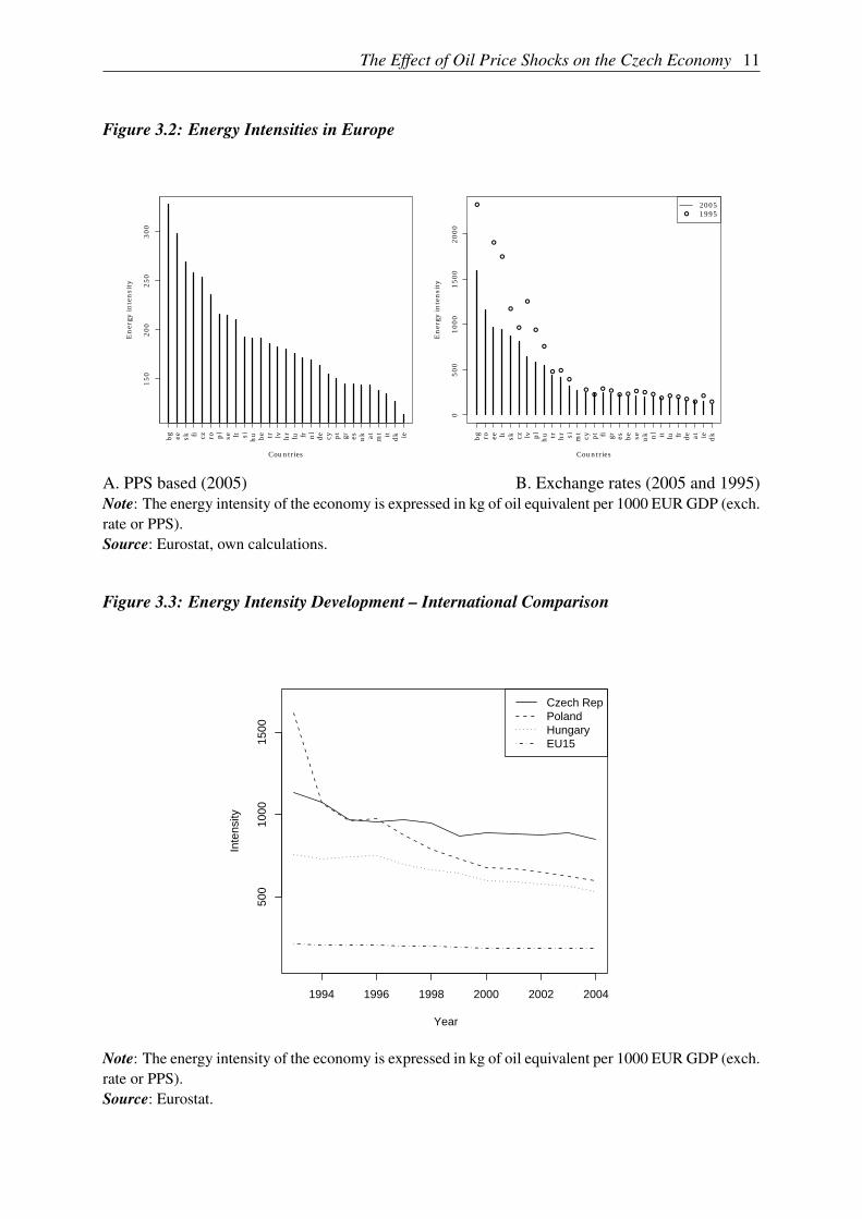
The Czech Republic ranks relatively high regarding energy intensity, with its 6th highest inten-sity within the EU25 group of countries. However, there has been an improvement compared tothe situation 10 years ago, see Figure 3.2. Table 3.3 shows that the energy intensity of the Czecheconomy has been declining almost continuously (though not much) over the past 10 years.Similar (or bigger) improvements in energy use can be observed for the other post-communistcountries (see Figure 3.3).
It is unclear whether the intensity improvements are mainly due to change in industrial structureor due to more efficient use within a given industry. Full decomposition is hard to achieve,since the energy use data is not available in the same industrial classification as the productiondata. Figure 3.4 shows the energy intensity changes in those industries where the energy andproduction classifications are compatible. These industries cover 70% of GDP. From the figurewe can conclude that within-industry energy intensity has been decreasing, so the aggregateintensity decrease is at least partly influenced by the within-industry intensity decrease. The
10 Kamil Dybczak, David Vonka and Nico van der Windt
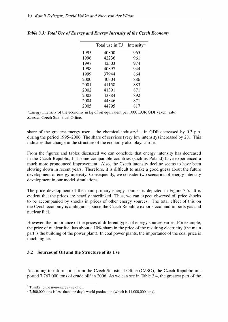
Table 3.3: Total Use of Energy and Energy Intensity of the Czech Economy
Total use in TJ Intensity*
1995 40800 9651996 42236 9611997 42503 9741998 40897 9441999 37944 8642000 40304 8862001 41158 8832002 41391 8712003 43884 8922004 44846 8712005 44795 817
*Energy intensity of the economy in kg of oil equivalent per 1000 EUR GDP (exch. rate).Source: Czech Statistical Office.
share of the greatest energy user – the chemical industry2 – in GDP decreased by 0.3 p.p.during the period 1995–2006. The share of services (very low intensity) increased by 2%. Thisindicates that change in the structure of the economy also plays a role.
From the figures and tables discussed we can conclude that energy intensity has decreasedin the Czech Republic, but some comparable countries (such as Poland) have experienced amuch more pronounced improvement. Also, the Czech intensity decline seems to have beenslowing down in recent years. Therefore, it is difficult to make a good guess about the futuredevelopment of energy intensity. Consequently, we consider two scenarios of energy intensitydevelopment in our model simulations.
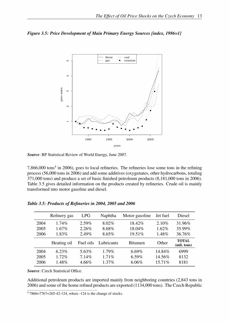
The price development of the main primary energy sources is depicted in Figure 3.5. It isevident that the prices are heavily interlinked. Thus, we can expect observed oil price shocksto be accompanied by shocks in prices of other energy sources. The total effect of this onthe Czech economy is ambiguous, since the Czech Republic exports coal and imports gas andnuclear fuel.
However, the importance of the prices of different types of energy sources varies. For example,the price of nuclear fuel has about a 10% share in the price of the resulting electricity (the mainpart is the building of the power plant). In coal power plants, the importance of the coal price ismuch higher.
3.2 Sources of Oil and the Structure of its Use
According to information from the Czech Statistical Office (CZSO), the Czech Republic im-ported 7,767,000 tons of crude oil3 in 2006. As we can see in Table 3.4, the greatest part of the
2 Thanks to the non-energy use of oil.3 7,500,000 tons is less than one day’s world production (which is 11,000,000 tons).
The Effect of Oil Price Shocks on the Czech Economy 11
Figure 3.2: Energy Intensities in Europe
Countries
En
ergy
in
ten
sity
bg ee sk fi cz ro pl
se lt si hu be tr lv hr lu fr nl
de cy pt
gr es uk at mt it dk ie
150
200
250
300
Countries
En
ergy
in
ten
sity
●
●
●
●
●
●
●
●
● ●
●
●●
● ●● ●
● ● ●● ● ●
●●
●
●
bg ro ee lt sk cz lv pl
hu tr hr si mt
cy pt fi gr es be se uk nl it lu fr de at ie dk
0500
1000
1500
2000
●
20051995
A. PPS based (2005) B. Exchange rates (2005 and 1995)Note: The energy intensity of the economy is expressed in kg of oil equivalent per 1000 EUR GDP (exch.rate or PPS).Source: Eurostat, own calculations.
Figure 3.3: Energy Intensity Development – International Comparison
1994 1996 1998 2000 2002 2004
500
1000
1500
Year
Inte
nsity
Czech RepPolandHungaryEU15
Note: The energy intensity of the economy is expressed in kg of oil equivalent per 1000 EUR GDP (exch.rate or PPS).Source: Eurostat.

12 Kamil Dybczak, David Vonka and Nico van der Windt
Figure 3.4: Intensities per Industry
1996 1998 2000 2002 2004
010
0020
0030
0040
00
Years
Inte
nsity
ChemicalNon−metalAgriculture
ServicesFoodPaper
Textile
Note: The energy intensity of the economy is expressed in kg of oil equivalent per 1000 EUR GDP (exch.rate or PPS).Source: Czech Statistical Office.
Czech oil supply comes from Russia. The typical type of oil for Czech refineries is thereforeheavy (high viscosity and density) and sour (high share of sulfur), i.e., of lower quality.
Table 3.4: Origins of Petroleum and Petroleum Product Imports in 2006 (Thousands of Tons)
Crude oil Motor gasoline Diesel oil
Russia 5225 — —Azerbaijan 1935 — —
Algeria 50 — —Libya 161 — —
Austria — 84 101Germany — 141 378Slovakia — 366 710
Other 396 24 65
Total 7767 615 1254
Source: Czech Statistical Office.
An additional 265,000 tons (of high quality oil) is produced in the Czech Republic, whichmakes the share of domestic production equal to 3.3%. The country exports negligible amountsof crude oil (42,000 tons in 2006). The rest, plus some stocks from the previous year (together
The Effect of Oil Price Shocks on the Czech Economy 13
Figure 3.5: Price Development of Main Primary Energy Sources [index, 1986=1]
1990 1995 2000 2005
12
34
5
years
pri
ce in
dex
●
●
● ●● ● ● ●
●
●
●● ●
●●
●●
●
●
●
●
Brentgas
coaluranium
Source: BP Statistical Review of World Energy, June 2007.
7,866,000 tons4 in 2006), goes to local refineries. The refineries lose some tons in the refiningprocess (56,000 tons in 2006) and add some additives (oxygenates, other hydrocarbons, totaling371,000 tons) and produce a set of basic finished petroleum products (8,181,000 tons in 2006).Table 3.5 gives detailed information on the products created by refineries. Crude oil is mainlytransformed into motor gasoline and diesel.
Table 3.5: Products of Refineries in 2004, 2005 and 2006
Refinery gas LPG Naphtha Motor gasoline Jet fuel Diesel
2004 1.74% 2.59% 8.02% 18.42% 2.10% 31.96%2005 1.67% 2.26% 8.68% 18.04% 1.62% 35.99%2006 1.83% 2.49% 8.65% 19.51% 1.48% 36.76%
Heating oil Fuel oils Lubricants Bitumen Other TOTAL(mil. tons)
2004 6.23% 5.63% 1.79% 6.69% 14.84% 69992005 1.72% 7.14% 1.71% 6.59% 14.56% 81322006 1.48% 4.66% 1.37% 6.06% 15.71% 8181
Source: Czech Statistical Office.
Additional petroleum products are imported mainly from neighboring countries (2,843 tons in2006) and some of the home refined products are exported (1134,000 tons). The Czech Republic4 7866=7767+265-42-124, where -124 is the change of stocks.

14 Kamil Dybczak, David Vonka and Nico van der Windt
exports mainly motor gasoline (293,000 tons), diesel (358,000 tons), and asphalt (135,000 tons).The major items of imported refined products are again motor gasoline (615,000 tons), diesel(1,254 tons), and asphalt (242,000 tons).
The structure of oil product use by industries is depicted in Figure 3.6. The share of transporthas been increasing and today forms the bulk of oil product use. Note that the use of oil productsin transportation also includes private car use by households. So, the households’ share onlycovers direct use for heating and so on and has therefore been negligible lately. The use ofoil for energy by industry has been decreasing, probably due to its price and substitutabilityby other energy-producing raw materials. The non-energy consumption is mainly due to thechemical industry (more than 50%). Non-energy oil consumption increased in the first part ofthe 1990s and has been stable since then.
Figure 3.6: Oil Product Use by Industry
1992 1994 1996 1998 2000 2002 2004
050
100
150
200
250
300
years
1000 t
eraj
oule
●
● ●
●
●
● ●●
● ●
●●
●
●
●
●
● ●
●
●
● ●
●
●●
●●
●●
●
● ●
Non−energyElectricity prodTransport
HouseholdsAgricultureIndustry
Source: Czech Statistical Office.
For modeling purposes, we can conclude as follows. The Czech Republic imports all its crudeoil needs. A negligible share is used for electricity and heat production; the rest is transformedto oil products, which form around 70% of the oil products on the market (the rest is importedfrom neighboring countries). The oil products are used for two main purposes: transport andnon-energy use in the chemical industry. Other sub-items are either negligible or are becomingnegligible at a high pace.
The Effect of Oil Price Shocks on the Czech Economy 15
3.3 The Price of Oil and its Decomposition
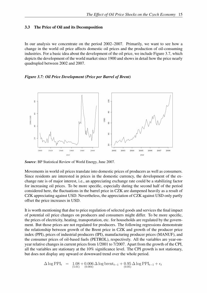
In our analysis we concentrate on the period 2002–2007. Primarily, we want to see how achange in the world oil price affects domestic oil prices and the production of oil-consumingindustries. For a basic idea about the development of the oil price, we include Figure 3.7, whichdepicts the development of the world market since 1900 and shows in detail how the price nearlyquadrupled between 2002 and 2007.
Figure 3.7: Oil Price Development (Price per Barrel of Brent)
1900 1920 1940 1960 1980 2000
20
40
60
80
year
2006 U
SD
2002 2003 2004 2005 2006 2007 2008
20
40
60
80
100
year
US
D
Source: BP Statistical Review of World Energy, June 2007.
Movements in world oil prices translate into domestic prices of producers as well as consumers.Since residents are interested in prices in the domestic currency, the development of the ex-change rate is of major interest, i.e., an appreciating exchange rate could be a stabilizing factorfor increasing oil prices. To be more specific, especially during the second half of the periodconsidered here, the fluctuations in the barrel price in CZK are dampened heavily as a result ofCZK appreciating against USD. Nevertheless, the appreciation of CZK against USD only partlyoffset the price increases in USD.
It is worth mentioning that due to price regulation of selected goods and services the final impactof potential oil price changes on producers and consumers might differ. To be more specific,the prices of electricity, heating, transportation, etc. for households are regulated by the govern-ment. But those prices are not regulated for producers. The following regressions demonstratethe relationship between growth of the Brent price in CZK and growth of the producer priceindex (PPI), prices of industrial producers (IPI), manufacturing producer prices (MANUF), andthe consumer prices of oil-based fuels (PETROL), respectively. All the variables are year-on-year relative changes in current prices from 1/2001 to 7/2007. Apart from the growth of the CPI,all the variables are stationary at the 10% significance level. The CPI growth is not stationary,but does not display any upward or downward trend over the whole period.
∆ log PPIt = 1.08(5.01)
+ 0.006(0.004)
∆ log brentt−1 + 0.95(0.05)
∆ log PPIt−1 + εt

16 Kamil Dybczak, David Vonka and Nico van der Windt
Figure 3.8: CZK/USD Exchange Rate since 2002
2002 2003 2004 2005 2006 2007 2008
20
25
30
35
years
CZK
/U
SD
Source: Czech National Bank.
∆ log IPIt = 35.13(23.48)
+ 0.018(0.010)
∆ log brentt−1 + 0.63(0.23)
∆ log IPIt−1 + εt
∆ log MANUFt = 46.61(31.87)
+ 0.023(0.013)
∆ log brentt−1 + 0.52(0.32)
∆ log MANUFt−1 + εt
∆ log PETROLt = 35.49(5.27)
+ 0.19(0.017)
∆ log brentt−1 + 0.44(0.06)
∆ log PETROLt−1 + εt
Indeed, the impact of CZK Brent prices on producer prices is most visible in petrol-relatedindustries. As the oil intensity of the industry in question decreases, we observe a lower impactof oil prices on the price of its output. In manufacturing, the short-run elasticity decreases to2.3%, since manufacturing includes many industries that use very little oil as an input. As weproceed to a more aggregate level (industry as a whole and the whole economy), the impact ofthe price of oil declines even more.
Price regulation alters the relation between oil import prices and domestic consumer prices.This is reflected by the fact that we found only a weak relationship between the domestic CPIand the price of Brent oil in CZK.
∆ log CPIt = 8.55(3.73)
+ 0.004(0.002)
∆ log brentt−1 + 0.91(0.036)
∆ log CPIt−1 + εt (3.1)
These results are obviously based on very simple models. A serious econometric analysis wouldrequire the use of a VAR model.
The Effect of Oil Price Shocks on the Czech Economy 17
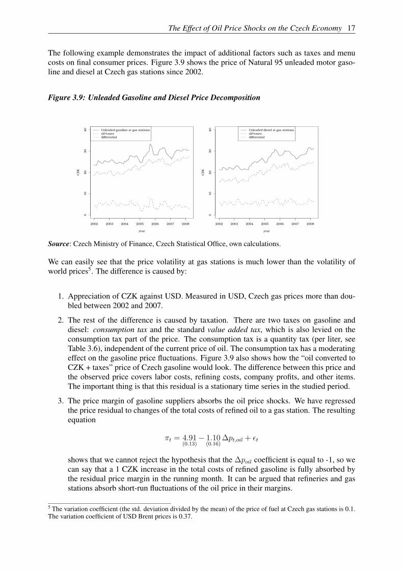
The following example demonstrates the impact of additional factors such as taxes and menucosts on final consumer prices. Figure 3.9 shows the price of Natural 95 unleaded motor gaso-line and diesel at Czech gas stations since 2002.
Figure 3.9: Unleaded Gasoline and Diesel Price Decomposition
2002 2003 2004 2005 2006 2007 2008
010
20
30
40
year
CZK
Unleaded gasoline at gas stationsoil+taxesdifferential
2002 2003 2004 2005 2006 2007 2008
010
20
30
40
year
CZK
Unleaded diesel at gas stationsoil+taxesdifferential
Source: Czech Ministry of Finance, Czech Statistical Office, own calculations.
We can easily see that the price volatility at gas stations is much lower than the volatility ofworld prices5. The difference is caused by:
1. Appreciation of CZK against USD. Measured in USD, Czech gas prices more than dou-bled between 2002 and 2007.
2. The rest of the difference is caused by taxation. There are two taxes on gasoline anddiesel: consumption tax and the standard value added tax, which is also levied on theconsumption tax part of the price. The consumption tax is a quantity tax (per liter, seeTable 3.6), independent of the current price of oil. The consumption tax has a moderatingeffect on the gasoline price fluctuations. Figure 3.9 also shows how the “oil converted toCZK + taxes” price of Czech gasoline would look. The difference between this price andthe observed price covers labor costs, refining costs, company profits, and other items.The important thing is that this residual is a stationary time series in the studied period.
3. The price margin of gasoline suppliers absorbs the oil price shocks. We have regressedthe price residual to changes of the total costs of refined oil to a gas station. The resultingequation
πt = 4.91(0.13)− 1.10
(0.16)∆pt,oil + εt
shows that we cannot reject the hypothesis that the ∆poil coefficient is equal to -1, so wecan say that a 1 CZK increase in the total costs of refined gasoline is fully absorbed bythe residual price margin in the running month. It can be argued that refineries and gasstations absorb short-run fluctuations of the oil price in their margins.
5 The variation coefficient (the std. deviation divided by the mean) of the price of fuel at Czech gas stations is 0.1.The variation coefficient of USD Brent prices is 0.37.

18 Kamil Dybczak, David Vonka and Nico van der Windt
Table 3.6: Consumption Tax and VAT on Gasoline and Diesel since 1995 [CZK/liter]
period Gasoline Diesel VAT
1995 7.62 22%1996-97 8.68 22%
1998-6/99 9.71 22%7/99-2003 10.84 8.15 22%
2004- 11.74 9.95 19%
Source: Ministry of Finance.
4. A General Equilibrium Model of the Czech Economy
In this section we present model simulation outcomes of oil price changes under several sce-narios. As mentioned already, the future energy intensity development in the Czech Republicis hard to predict. On the one hand there is a sizeable gap between the current Czech energyintensities and those of the EU15. This suggests that the Czech economy might be able to catchup within the not too distant future. On the other hand, the past development (see Figure 3.3)shows that the intensity decline has been rather slow during the last decade (on average 2% p.a.)and even decelerating in the last 5 years.
Also, there is substantial uncertainty about the impact of oil prices on the Czech Republic’strade partners, especially the EU. Therefore, in our simulations we concentrate on differentassumptions about the development of technology and world demand.
We first simulate the impact of an oil price change under the assumption of no change in oilintensity (pessimistic scenario), assuming that the impact on the Czech Republic’s trade partnerswill be in line with the literature results summarized in Section 5.
Then we compare the results with other simulations where we assume no impact of the oil priceshock on economies other than the Czech one. At first sight, this seems to be an unrealisticassumption. But taking into account the relatively low energy intensity of the EU15 economies(by far the greatest trade partners of the Czech Republic), we could argue that the oil price effecton them is of a limited extent and importance for our calculations.
In the third simulation we compare the results of the first simulation with the same simulationunder the assumption of reaching the EU15 energy intensity levels in 10 years.
Our general conclusion is that regardless of alternative simulation assumptions, the effects of oilprice increases are rather small, though rather bigger than the impacts suggested, for example,by equation (3.1) in the empirical part of this paper.

The Effect of Oil Price Shocks on the Czech Economy 19
4.1 Oil Price Shock in the Model
Before running the simulations, it is worthwhile to review the structure of the model from thepoint of view of the shock that is to be studied. This section describes how oil price shocksdisseminate through the model. A more complete description of the model is presented inAppendix B.
To capture the propagation mechanism of an oil price shock, we start with equation
Pmc,t = ERt(1 + τmc,t)P
wc,t, (4.2)
where Pmc,t represents the import price of commodity c at time t in CZK including import tariffs,
ERt is the exchange rate, τmc,t stands for the rate of tariffs, indirect taxes, transport, and otherimport-related costs, and Pw
c,t denotes the world price in foreign currency. The world price isassumed exogenous to the model, since we model a small open economy. The development ofthe exchange rate is also assumed to be exogenous. It is worth stressing that equation (4.2) isthe only one where the world oil price explicitly enters the model.
Import prices directly influence prices of intermediates, which are both imported and produceddomestically. We assume that firms have to import a certain share of their intermediates fromabroad (Leontief production structure). The price of intermediates paid by industry i is definedas a weighted average of the domestic and import prices of the intermediate commodities.
P inti,t =
∑c
(P dc,tINTd
i,c,t + Pmc,tINTm
i,c,t
)∑c INTi,c,t
(4.3)
The intermediate price enters the price of domestic production
P domi,t = (1 + markupi)
wi,tLi,t + rtKi,t + P inti,t INTi,t
Qdomi,t
, (4.4)
where P domi,t represents the unit price of domestic producers, markup stands for the profit margin,
wi,t denotes the wage level, Li,t is employment in industry i, rt is the real interest rate, Ki,t isthe capital stock, INTi,t is intermediate consumption, and P int
i,t is its price. Together, importprices and domestic producer prices determine the price level CPIt on the Czech market.
Contrary to firms, households are assumed to be able to substitute imported goods for domesticones and vice versa if relative prices change.
Cdomc,t
Cmc,t
=
(αc
1− αcPmc,t
P domc,t
) 11+σc
(4.5)
Here, Cc,t is the household consumption of commodity c at time t, αc is a calibrated coeffi-cient, and σc is the relative price elasticity of household demand (we set σc around 2 for mostcommodities).

20 Kamil Dybczak, David Vonka and Nico van der Windt
The CPI is influenced by both domestic and import prices.
CPIt =
∑c
(P domc,t Cdom
c,t + Pmc,tC
mc,t
)∑c
(Cdomc,t + Cm
c,t
) (4.6)
An increase in the price level puts pressure on wages. The wage equation is a fundamentalbuilding block of the model. It says that
∆ logwi,t = ∆ log CPIt + ∆ log hi,t −λiut, (4.7)
where hi,t is the productivity level in industry i, ut is the unemployment rate, and λi > 0. Thewage equation says that wages reflect price and productivity developments but get moderatedif unemployment starts to grow (Phillips curve effect). When consumer prices change, wageschange ceteris paribus by the same relative amount. Prices of domestic producers are affectedagain by a wage level change.
We assume that Czech producers do not price discriminate between the Czech and foreignmarket, thus the export price is just the domestic price converted to foreign currency:
P expc,t = ERtP
domc,t (4.8)
The external demand for Czech products is influenced by the ratio of world prices to Czechexport prices, i.e.
∆ log EXPc,t = ∆ log GDPworldt + σεc
[∆ log Pworld
c,t −∆ log Pexpc,t
](4.9)
where σεc is around 1.7 for most commodities.
Indeed, as the domestic export price rises, the competitiveness of the economy deteriorates. Itfollows that real exports and thereby aggregate demand for Czech production decrease.
The production side of the economy is hit by the cost shock in several ways
1. Prices of intermediate goods increase. In the model intermediate goods cannot be substi-tuted for labor and capital.
2. The increased wages push up labor costs.
3. Prices of capital goods grow as well (by the same mechanism as prices of intermediates)and the decreased demand for domestic production leads to a fall in the optimal capitalstock. This leads to lower investment and a further demand decline.
All in all, demand for domestic output decreases and firms adjust their labor force. The resultingunemployment leads to wage moderation (see equation (4.7)) and a decrease in productioncosts. In the long run, Czech production becomes competitive again, but the cost structurechanges. The cost share of imported goods increases and the share of labor costs decreases.The terms of trade deteriorate and real household income is lower in the new equilibrium.In quantities, we will import less and export more, keeping a roughly stable current accountbalance in the long run. The loser in this scenario is households, whose incomes are cut in orderto regain competitiveness.

The Effect of Oil Price Shocks on the Czech Economy 21
4.2 Presentation of Simulation Results
The simulation results are presented in Tables 4.1, 4.2, and 4.3. Each table presents eight eco-nomic indicators. Except for the CPI, all the variables are given in real terms (fixed prices). Thelast two rows represent the cumulative present value loss of GDP and household consumptionover 1, 3, and 5 years and the infinite horizon expressed as a percentage of GDP and house-hold consumption respectively in the first year. To compute the cumulative losses we applya 3% p.a. discount rate. The cumulative present value consumption loss is therefore definedby Lc = 1
Cbase1
∑+∞t=1
Ct−Cbaset
(1+0.03)t. The expression for the cumulative present value GDP loss is
analogous.
A series of four permanent oil price shocks enters the model in years 1, 2, 3, and 4. The tablespresent the results in years 1, 3, and 5 and in the long run (column +∞). The precise definitionsof the alternative simulations are provided in the respective subsections.
The presented figures denote a difference from the baseline. The baseline always equals 100.So, for example, 99.2 in the upper-right corner of Table 4.1 means that in Simulation 1 realGDP will be 0.8% lower in the long run than it would be if no price shock occurred.
Similarly, in the fourth row, first column of Table 4.1 the figure 99.6 indicates that in the firstsimulation real exports will be 0.4% lower in the first year of the shock compared to the baseline.
4.3 Simulation 1: Overall Increase in Oil Prices
In this simulation we assume that import prices of oil and oil products in Czech koruna increaseby 5% a year during the upcoming 4 years, i.e., by 20% over this horizon. In all following yearsthe price of oil stays at the level of year 4. Since the oil price has increased by around 50% inthe last five years (see Figure 3.9), this shock seems to be within realistic bounds. The relatedprices of imported chemical products are assumed to increase by 0.8% a year during the fouryears. In this scenario, the oil price shock hits both the Czech economy and its trade partners,therefore world market prices of all goods are assumed to increase. Aggregate world demand(i.e., also world demand for Czech goods) is also assumed to decrease. Within this scenario, nooil intensity improvement is taken into account, either in the Czech Republic or abroad.
Since the model is not a two-country model, the assumptions about the impact of oil prices onthe Czech Republic’s trade partners are bound to be arbitrary. We assume a world price increasedue to an oil price shock in the range of 0 to 1% in the long run, depending on the characteristicsof the goods traded. Furthermore, we assume that the oil price shock cuts aggregate worlddemand by around 0.2%. This is roughly in line with the literature (see, for example, the surveyby Kingma and Suyker (2004)). Alternative sensitivity scenarios suggest that the results are notsignificantly affected by assuming a higher impact on foreign economies6 (see Table A.4).
It is worth emphasizing that the impact on the foreign country has two effects on the CzechRepublic, which can be of opposite sign. First, the decrease in world demand is simply a6 An alternative scenario assuming a 1% foreign demand decrease instead of the original 0.2% decrease was sim-ulated.

22 Kamil Dybczak, David Vonka and Nico van der Windt
Table 4.1: Results of Simulation 1: Overall Increase in Oil Price
1 3 5 +∞GDP 99.5 98.8 98.5 99.2Household consumption 99.6 99.0 98.8 97.5Gross investment 98.3 96.4 96.6 98.3Export 99.6 98.7 98.3 101.4Import 99.4 98.7 98.5 98.9Employment 99.1 97.8 97.7 100.2CPI 100.4 101.5 102.1 99.5Gross wage 100.1 100.2 100.2 96.1
GDPcumul -0.5 -2.5 -5.3 -40.8Household consumptioncumul -0.4 -2.1 -4.2 -78.3
Note: Column “1” corresponds to the first year of the shock, “3” to the third year of the shock, “5” to thefifth year (one year after the shock) and “+∞” to the long-run result. The presented figures are indexnumbers where the baseline scenario equals 100. The last two rows report the cumulative present valueloss of GDP and household consumption as percent of GDP and household consumption, respectively,in the base year. A 3% discount rate is used.Source: Own calculations.
negative shock for the Czech economy. Second, the world price level increase would ceterisparibus have a positive impact on Czech competitiveness. But at the same time higher importprices increase domestic costs and price levels. The net effect depends on the relation of importsto exports in each commodity group.
The oil price shock first hits domestic oil importers. Simultaneously, all other domestic im-porters face higher prices due to the oil-induced price level increase abroad. Both groups ofimporters pass on the increased costs to their prices, which in turn increases the costs (andprices) of their customers and the prices of final goods. The simulated price level impact of theoil price shock is rather moderate: the CPI gap is 0.4% in the first year and 2.1% after 5 years.This amounts to an average oil shock net impact of around 0.4 p.p. extra inflation in the first 5years.
The higher level of domestic prices has a negative effect on both international competitivenessand domestic demand. GDP will be roughly 1.5% lower in the fifth year, i.e., after the wholeshock is realized. So in the short run, average domestic economic growth slows down by 0.3%per year. Lower economic performance and higher nominal wages are accompanied by a dropin aggregate employment by 2% in the short run.
As already mentioned in Section 4.1, in the first years real wages are not strongly affectedby the decrease in employment. On the contrary, real wages increase slightly in reaction toproductivity increases triggered by the employment cuts. Later on, the bargaining power ofemployees deteriorates, which leads to a real wage decrease. This allows cost and price cuts,more employment and restoration of the competitive position of the economy. Exports riseabove their pre-shock levels, while imports remain low. In the nominal terms this leads toan equilibrium balance of payments under the new (worse) terms of trade. The burden of theshock is borne by households, whose income is cut in order to regain competitiveness. This

The Effect of Oil Price Shocks on the Czech Economy 23
mechanism is reflected in the cumulative household consumption loss being much higher thanthe cumulative loss of GDP.
Compared to the baseline, the CPI decreases in the long run as a result of the wage cuts. Thesimulated long-run effect on the GDP level seems to be rather limited, at around −0.8%. Thelong-run model outcomes reflect the restored competitiveness and employment.
The impact of the oil price change partly depends on the reaction of the government. Weassume that the government does not try to keep the budget balanced in the years of the shock.Later (after 10 years) it cuts down its consumption to reach public finance sustainability. Otherassumptions about the government reaction are introduced in the form of a robustness check inthe Appendix (see Table A.4).
4.4 Simulation 2: Isolated Increase in Oil Price
In this simulation we again assume that import prices of oil and oil products in Czech korunaincrease by 5% a year during the upcoming 4 years, i.e., by 20% over this horizon. The relatedprices of imported chemical products are assumed to increase by 0.8% a year during the fouryears. In this simulation we still assume that the intensity of oil use does not change beyond the(rather limited) substitution possibilities assumed in the production structure of our model. Thedifference from the base simulation is that we assume that the oil price increase hits the Czecheconomy only. The aim of this simulation is to show which part of the result of Simulation 1 iscaused by the assumptions about the foreign reaction. For another simulation which considersa larger impact on foreign economies, see the robustness analysis in the Appendix.
Table 4.2: Results of Simulation 2: Isolated Increase in Oil Price
1 3 5 +∞GDP 99.6 98.8 98.5 99.2Household consumption 99.7 99.0 98.8 97.5Gross investment 98.6 96.6 96.7 98.3Export 99.6 98.7 98.2 101.4Import 99.5 98.7 98.5 98.8Employment 99.2 97.9 97.6 100.2CPI 100.3 101.2 101.7 99.0Gross wage 100.1 100.2 100.2 96.1
GDPcumul -0.4 -2.4 -5.2 -41.3Household consumptioncumul -0.4 -1.9 -4.1 -79.3
Note: Column “1” corresponds to the first year of the shock, “3” to the third year of the shock, “5” to thefifth year (one year after the shock) and “+∞” to the long-run result. The presented figures are indexnumbers where the baseline scenario equals 100. The last two rows report the cumulative present valueloss of GDP and household consumption as percent of GDP and household consumption, respectively,in the base year. A 3% discount rate is used.Source: Own calculations.

24 Kamil Dybczak, David Vonka and Nico van der Windt
The difference between Simulation 1 and Simulation 2 is apparent in the development of infla-tion. In the long run the price level is 1% below the baseline scenario. In Simulation 1 it was1.5% below. Concerning GDP, the difference between the two scenarios is very limited andpresent only in the very short run. We conclude that taking into account the reactions of the restof the world to an oil price shock increases the impact on the domestic price level, but does notinfluence aggregate economic activity.
All in all, the results of Simulations 1 and 2 are rather similar. This is due to the contradictoryimpact of the foreign demand drop and the foreign price increase on Czech competitiveness.
4.5 Simulation 3: Increase in Oil Price under Energy Intensity Improvement
In this simulation we again assume that import prices of oil and oil products in Czech korunaincrease by 5% a year during the upcoming 4 years, i.e., by 20% over this horizon. The relatedprices of imported chemical products are again assumed to increase by 0.8% a year duringthe four years. The difference from Simulation 1 is that the oil use intensity is assumed toimprove by 5.5% a year between years 1 and 10. Over the 10 years, the intensity is thusassumed to improve by 71%, which would close the gap between the EU15 and the Czechenergy intensity levels (see Figure 3.3). In other words, this simulation assumes that the CzechRepublic converges to the EU15 rather rapidly in terms of energy intensity.
Table 4.3: Results of Simulation 3: Increase in Oil Price under Energy Intensity Improve-ment
1 3 5 +∞GDP 99.6 99.1 99.0 99.4Household consumption 99.7 99.3 99.2 98.3Gross investment 98.7 97.5 97.7 98.8Export 99.7 99.1 98.9 100.9Import 99.5 99.0 99.0 99.2Employment 99.3 98.5 98.4 100.1CPI 100.3 101.1 101.6 99.8Gross wage 100.1 100.2 100.1 97.4
GDPcumul -0.4 -1.8 -3.7 -27.2Household consumptioncumul -0.3 -1.5 -3 -53.8
Note: Column “1” corresponds to the first year of the shock, “3” to the third year of the shock, “5” to thefifth year (one year after the shock) and “+∞” to the long-run result. The presented figures are indexnumbers where the baseline scenario equals 100. The last two rows report the cumulative present valueloss of GDP and household consumption as percent of GDP and household consumption, respectively,in the base year. A 3% discount rate is used.Source: Own calculations
Intuitively, thanks to the lower oil use intensity, the impact of the oil price shock on the Czecheconomy is less pronounced. Otherwise, the mechanisms described in Simulation 1 still apply.

The Effect of Oil Price Shocks on the Czech Economy 25
To interpret the results of this simulation it is necessary to emphasize that the reduction in oilintensity is assumed to be compensated by an increase of use of other inputs, whose pricesincrease much less. In other words, importing less oil means importing (and paying) more ofsome other input in order to produce the same amount of output.
The most pronounced improvements compared to Simulation 1 can be observed in householdconsumption and wages. As described in Section 4.1, households bear the final burden of theprice shock, since their employment (in the short run) and wages (in the long run) decrease.The dampening of the shock via technological progress is therefore beneficial to them.
The decrease in real wages is much smaller than in Simulation 1 (2.6% against 3.9% in the longrun). Households enjoy higher real income and therefore spend more on imported goods. Realexports increase less than without the technological progress and imports are higher, thereforethe exports deteriorate compared to Simulation 1. The final effect on GDP is therefore lesspronounced than the effect on domestic demand and wages.
5. Impact of Oil Price Shock in Other Models
During recent years several institutions have carried out analyses of oil price changes on pricesand economic activity using their economic models. Such analyses have been undertaken by in-stitutions such as the ECB (AWM model), the IMF (Multimod model), the EC (QUEST model),the OECD (Interlink model), and the NIESR (NiGEM model), to name but a few. Indeed, itshould be borne in mind that each model is partly based on different assumptions and possiblystresses the role of alternative factors and relationships. Regardless of such differences, thesimulation outcomes point in same direction and the main conclusions seem to be robust to themodeling practices applied.7
Table 5.1: Model Comparison
Inflation GDP growthYear 1 Year 3 Year 1 Year 3
ECB AWM 0.5 0.1 -0.1 -0.1EC QUEST 0.4 0.1 -0.6 -0.1NiGEM 0.3 0.0 -0.8 0.1IMF Multimod 1.6 0.5 -0.1 0.1Our model 0.8 0.9 -1.0 -1.0
Note: Reaction to a 50% permanent oil price increase.
The European Commission QUEST model does not treat oil as a separate commodity. The oilprice shock is simulated indirectly via an increase in import prices, using the relative importanceof net imports of oil in total imports. The simulated impact on inflation is 0.4 p.p. above thebaseline in the first year and 0.1 p.p. in the third year in reaction to a permanent increase in oil
7 For a more detailed comparison of oil price change simulations on prices and economic activity, see, for example,ECB (2004).

26 Kamil Dybczak, David Vonka and Nico van der Windt
prices of 50%. The impact on GDP growth under the same assumptions was simulated to be-0.6 and -0.1 p.p. lower relative to the base scenario. The simulation outcomes of the NIGEMmodel are relatively close to the QUEST outcomes in suggesting an increase in inflation of 0.3and 0.0 p.p. in the first and third year, respectively. The impact on GDP growth is -0.8 and 0.1p.p. compared to the baseline scenario.
The AWM model estimates suggest that a permanent 50% rise in oil prices adds to overallinflation by 0.5 p.p. within the first year. After three years overall inflation would be 0.1 p.p.higher compared with the situation of unchanged oil prices. Regarding economic activity, theAWM model suggests that a 50% increase in oil prices would lead to real GDP growth decliningby 0.1 p.p. in the first year. Likewise, this model predicts an impact of -0.1 p.p. in the thirdyear.
The IMF Multimod is driven mainly by longer-term relationships. That is probably why themodel yields stronger effects than the other models. The impact of a 50% oil price shock issimulated to be 1.6 and 0.5 p.p. on inflation and -0.1 and 0.1 p.p. on GDP growth in the firstand third year, respectively.
As already mentioned, our model puts more weight on the detailed structure of the economywhile leaving out some important dynamic features such as expectations and intertemporal op-timization. The lack of intertemporal smoothing leads to higher effects of shocks in the shortrun, as can be seen in the effect on GDP in comparison with other models. There are severalother reasons why our model reports higher deviations from the baseline scenario in the shortrun. Firstly, the absolute size of the 50% is much higher in our simulation, as the oil pricein our baseline reflects the recent high oil prices. Secondly, in the other models oil-exportingcountries are assumed to spend most of their oil profits on imports from the simulated countries.That is how the GDP effect can turn out positive after three years. Thirdly, the Czech energyintensity is higher than that of the EU and the US, so we do expect higher effects. Anyway, themain conclusions of our analysis seem to be in line with the outcomes of the models mentionedabove.
6. Concluding Remarks
The paper was motivated by the dramatic increases in oil prices recorded in the course of 2002up to the end of 2007. The USD price of one barrel of Brent oil increased during the analysedperiod more than five times. This has triggered a debate among Czech economists about thepossible impacts of such a price shock on the Czech economy. In our study we use severalapproaches to show that the impact of such a shock is not dramatic. Our arguments can besummarized as follows.
First, the structure of energy use in the Czech Republic reflects the fact that some energy sources(e.g. coal) are abundant in the Czech Republic. This results in low overall energy dependence.On the other hand, the energy intensity of the Czech economy is much higher than that in theEU15. The USD price of a barrel of Brent is not the only determinant of the price paid bythe Czech consumer. The price can be moderated by appreciation of CZK, which has been thecase in recent years. The volatility of the oil price is also restricted by the construction of theconsumption tax system.
The Effect of Oil Price Shocks on the Czech Economy 27
Second, reduced-form regressions of different price measures on the oil price confirm thatCzech prices react very little to oil price developments. The long-run effect of an oil priceincrease of 1% on the PPI was estimated to be 0.12%. For the CPI the figure is 0.044%. Theestimated elasticity of the CPI is lower due to energy price regulation and the absorption ofshort-run oil price fluctuations by producers.
Third, structural CGE model simulations indicate that the impact of oil prices on both nominaland real variables is not too high, although the effects are higher than those reported for the EUand the USA in the literature. We present three alternative simulations. In the base simulation,both the Czech Republic and its trade partners are hit by the shock. In the second scenario,only the Czech Republic is hit by the shock. In the third scenario, the impact of the shock ismitigated by technological improvement.
On basis of these simulations we predict that a 20% rise in the price of oil in Czech korunawould slow economic growth down by around 0.4 p.p. per year in the first years after theshock. The shock would decrease the long-run GDP level by around 0.7%. In the short run,inflation would also increase by around 0.4 p.p. per year. In the long run, the price level wouldactually decline compared to the scenario without a shock. This decrease is caused by wagecuts necessary to restore international competitiveness.
To check the robustness of the results we performed several alternative simulations. The resultsof these simulations indicate that our results are reasonably robust.

28 Kamil Dybczak, David Vonka and Nico van der Windt
References
ADELMAN, I. AND ROBINSON, S. (1977): Income Distribution and Poverty in DevelopingCountries. Stanford University Press.
CARRUTH, A., HOOKER, M., AND OSWALD, A. (1993): “Unemployment, Oil Prices and theReal Interest Rate: Evidence from Canada and the UK.” Technical report, University ofGuelph.
CHUMACERO, R. A. AND SCHMIDT-HEBBEL, K. (2004): “General Equilibrium Models: AnOverview.” Working Papers Central Bank of Chile 307, Central Bank of Chile.
COADY, D. P. AND HARRIS, R. L. (2001): “A Regional General Equilibrium Analysis ofthe Welfare Impact of Cash Transfers: An Analysis of PROGRESA in Mexico.” TMDDiscussion paper 76, International Food Policy Research Institute, Washington.
DG-ECFIN (2005): “Assesing the Economic Impact of the Continuing Increase in Oil Prices.”Technical report REP 53748/05, European Commission.
DG-ECFIN (2005): “The Impact of Higher Oil Prices, Developments after the Finalisation ofthe Commission Forecast.” Technical report REP 51952/05, European Commission.
DG-ECFIN (2005): “Oil and Energy Markets: Recent Developments, Outlook, Dialogueswith Producer Countries, and Data Issues.” Technical report REP 55442/05, EuropeanCommission.
DG-ECFIN (2005): “Energy Efficiency in the EU: Trends, Driving Forces, Outlook.” Tech-nical report, European Commission.
ECB (2004): “Oil Prices and the Euro Area Economy.” ECB Monthly Bulletin, ECB.
GTAP (2006): “Global Trade Analysis Project.” Technical report, Center for Global TradeAnalysis, Purdue University.
HAMILTON, J. (1983): “Oil and the Macroeconomy Since World War II.” Journal of PoliticalEconomy, 91:228–248.
HLEDIK, T. (2003): “Modelling the Second-Round Effects of Supply-Side Shocks on Infla-tion.” Working Papers 2003/12, Czech National Bank, Research Department.
IMF, editors. (2005): World Economic Outlook, chapter Chapter IV: Will the Oil MarketContinue to be Tight? pages 157–183. International Monetary Fund.
JIMENEZ-RODRIGUEZ, E. AND SANCHEZ, M. (2004): “Oil Price Shocks and Real GDPGrowth: Empirical Evidence for Some OECD Countries.” Working paper 362, ECB.
JOHANSEN, L. (1960): A Multi-Sectoral Study of Economic Growth. North Holland.
KEANE, M. P. AND PRASAD, E. S. (1991): “The Employment and Wage Effects of Oil PriceShocks: A Sectoral Analysis.” Discussion paper 51, Institute of Empirical Macroeco-nomics, Federal Reserve Bank of Minneapolis.
KINGMA, D. AND SUYKER, W. (2004): “FAQs about oil and the world economy.” CPBMemoranda 104, CPB Netherlands Bureau for Economic Policy Analysis available athttp://ideas.repec.org/p/cpb/memodm/104.html.

The Effect of Oil Price Shocks on the Czech Economy 29
SMID, B. (2006): “Athena - A multi-sector model of the Dutch economy.” Technical report,CPB.
WALRAS, L. (1926): Elements d’economie politique pure. Paris: Pichon et Durand-Auzias,definitive, revue et augmentee par l’auteur edition.
WILLIAMS, J. L. (2006): “Oil Price History and Analysis.” In Energy Economics Newsletter.

30 Kamil Dybczak, David Vonka and Nico van der Windt
Appendix A
Robustness Check
The results reported in tables 4.1, 4.2, and 4.3 depend on a set of assumptions and parametervalues discussed in appendix B. Here we discuss the parameters and assumptions that might beimportant for the results and perform the respective robustness checks.
In table A.1, the effect of changes of the Phillips curve parameter (λ in Appendix B) is studied.The Phillips curve parameter is responsible for the link between unemployment and wages.If the parameter is high, unemployment leads to a bigger decrease of the bargaining power ofemployees and real wages decrease faster. Assuming less flexibility leads to higher inflation andless economic growth. In the table we report simulations where the Phillips curve parameter ishalved (compared with the simulations presented in sections 4.3 to 4.5). The scenario includeshigher inflation and less growth, but the impact is moderate.
Other parameters of interest are import and export elasticities. Export elasticities describe thesensitivity of foreign demand to Czech price setting. Import elasticities describe the reactionsof Czech private consumption demand to changes in foreign prices. The results for doubledand halved elasticities are reported in tables A.2 and A.3 for export and import, respectively.The effect of assumptions about import elasticities on our results is negligible. The exportelasticities tend to be more important. In each simulation, the economy adjusts the level of realwages to reestablish competitiveness. When the export elasticities are lower wages must be cutmore, which leads to the negative effects observed in table A.2.
Further, in line with the model results of other institutions (see table 5.1), we assumed that theeffect of oil prices on foreign GDP (i.e., aggregate world demand) would be negligible afterthree years. These model results seem to be very optimistic. Therefore, as a robustness check,we also report results based on a long-run aggregate world demand decrease of 1% (instead of0.2% in the base simulation), much above any published estimate. The result given in the secondblock of table A.4 indicates that the simulation result is not overly sensitive to this parameter.
Another possible uncertainty is about the role of the government budget. In any case, the gov-ernment must sooner or later balance its budget, so a certain amount of restriction is inevitable.In the base simulation we assume that the government postpones stabilization of its budgets by10 years so that the primary negative effects of the shock phase out, and then it slowly decreasesits consumption to attain a balanced budget. As a robustness check we run simulations whereincome tax and VAT are increased instead of the consumption cuts. The income tax increaseshave relatively negative effects on overall economic activity, while the VAT closure increasesthe negative impact on the price level. The results are given in table A.4.

The Effect of Oil Price Shocks on the Czech Economy 31
Tabl
eA
.1:T
heR
obus
tnes
sRes
ults
with
Res
pect
toth
eR
elat
ions
hip
betw
een
Wag
eB
arga
inin
gPo
wer
and
Une
mpl
oym
ent
Oil
pric
ein
crea
seon
lyin
CZ
Oil
pric
ein
crea
seev
eryw
here
and
tech
.im
prov
emen
t
Oil
pric
ein
crea
seev
eryw
here
13
5+∞
13
5+∞
13
5+∞
Base
GD
P99
.698
.898
.599
.299
.699
.199
99.4
99.5
98.8
98.5
99.2
Hou
seho
ldco
nsum
ptio
n99
.799
98.8
97.5
99.7
99.3
99.2
98.3
99.6
9998
.897
.5G
ross
inve
stm
ent
98.6
96.6
96.7
98.3
98.7
97.5
97.7
98.8
98.3
96.4
96.6
98.3
Exp
ort
99.6
98.7
98.2
101.
499
.799
.198
.910
0.9
99.6
98.7
98.3
101.
4Im
port
99.5
98.7
98.5
98.8
99.5
9999
99.2
99.4
98.7
98.5
98.9
Em
ploy
men
t99
.297
.997
.610
0.2
99.3
98.5
98.4
100.
199
.197
.897
.710
0.2
CPI
100.
310
1.2
101.
799
100.
310
1.1
101.
699
.810
0.4
101.
510
2.1
99.5
Gro
ssw
age
100.
110
0.2
100.
296
.110
0.1
100.
210
0.1
97.4
100.
110
0.2
100.
296
.1
Phillipseffecthalved
GD
P99
.698
.798
.398
.899
.699
.198
.899
.399
.598
.798
.398
.9H
ouse
hold
cons
umpt
ion
99.6
99.1
9997
.699
.699
.399
.398
.399
.699
.199
.197
.6G
ross
inve
stm
ent
98.6
96.6
96.6
98.2
98.6
97.4
97.6
98.7
98.3
96.4
96.6
98.1
Exp
ort
99.6
98.5
97.8
101
99.6
9998
.510
0.7
99.5
98.5
97.8
101
Impo
rt99
.598
.798
.498
.799
.599
98.9
99.1
99.4
98.6
98.4
98.7
Em
ploy
men
t99
.297
.797
.399
.799
.298
.498
.299
.899
97.7
97.4
99.7
CPI
100.
410
1.3
102
99.3
100.
410
1.3
101.
910
010
0.4
101.
610
2.4
99.8
Gro
ssw
age
100.
110
0.5
100.
796
.510
0.1
100.
310
0.5
97.6
100.
210
0.5
100.
896
.5
Phillipseffectdoubled
GD
P99
.699
98.8
99.2
99.7
99.3
99.3
99.5
99.6
9998
.999
.2H
ouse
hold
cons
umpt
ion
99.6
98.9
98.6
97.6
99.6
99.1
9998
.499
.698
.898
.597
.7G
ross
inve
stm
ent
98.7
96.7
96.9
98.4
98.7
97.6
97.8
98.9
98.3
96.6
96.8
98.4
Exp
ort
99.7
99.1
9910
1.2
99.8
99.5
99.5
100.
899
.799
.299
.210
1.1
Impo
rt99
.598
.898
.698
.999
.699
.199
.199
.299
.598
.798
.798
.9E
mpl
oym
ent
99.3
98.2
98.3
100.
299
.398
.798
.910
0.1
99.1
98.2
98.3
100.
2C
PI10
0.3
100.
810
199
.210
0.3
100.
910
1.1
100
100.
310
1.1
101.
499
.7G
ross
wag
e10
099
.899
.296
.310
099
.799
.397
.510
099
.799
.296
.4

32 Kamil Dybczak, David Vonka and Nico van der Windt
Tabl
eA
.2:T
heR
obus
tnes
sRes
ults
with
Res
pect
toPr
ice
Ela
stic
ities
ofE
xpor
t
Oil
pric
ein
crea
seon
lyin
CZ
Oil
pric
ein
crea
seev
eryw
here
and
tech
.im
prov
emen
t
Oil
pric
ein
crea
seev
eryw
here
13
5+∞
13
5+∞
13
5+∞
Base
GD
P99
.698
.898
.599
.299
.699
.199
99.4
99.5
98.8
98.5
99.2
Hou
seho
ldco
nsum
ptio
n99
.799
98.8
97.5
99.7
99.3
99.2
98.3
99.6
9998
.897
.5G
ross
inve
stm
ent
98.6
96.6
96.7
98.3
98.7
97.5
97.7
98.8
98.3
96.4
96.6
98.3
Exp
ort
99.6
98.7
98.2
101.
499
.799
.198
.910
0.9
99.6
98.7
98.3
101.
4Im
port
99.5
98.7
98.5
98.8
99.5
9999
99.2
99.4
98.7
98.5
98.9
Em
ploy
men
t99
.297
.997
.610
0.2
99.3
98.5
98.4
100.
199
.197
.897
.710
0.2
CPI
100.
310
1.2
101.
799
100.
310
1.1
101.
699
.810
0.4
101.
510
2.1
99.5
Gro
ssw
age
100.
110
0.2
100.
296
.110
0.1
100.
210
0.1
97.4
100.
110
0.2
100.
296
.1
Exportelasticitieshalved
GD
P99
.799
.399
.198
.699
.799
.499
.399
99.6
99.2
99.1
98.6
Hou
seho
ldco
nsum
ptio
n99
.899
.499
.496
.399
.799
.599
.697
.399
.699
.499
.396
.2G
ross
inve
stm
ent
99.2
98.2
98.3
9799
98.5
98.7
97.9
98.7
97.9
98.1
96.9
Exp
ort
99.8
99.3
9910
1.6
99.7
99.4
99.2
101.
199
.799
.298
.910
1.6
Impo
rt99
.799
.399
.398
99.7
99.4
99.4
98.5
99.6
99.2
99.2
97.9
Em
ploy
men
t99
.598
.798
.610
0.2
99.4
9999
100.
299
.398
.698
.510
0.2
CPI
100.
410
1.3
101.
897
.510
0.4
101.
310
1.7
98.5
100.
510
1.6
102.
397
.8G
ross
wag
e10
010
0.2
100.
294
.210
010
0.1
100.
295
.710
010
0.2
100.
294
Exportelasticitiesdoubled
GD
P99
.498
.197
.699
.399
.698
.898
.699
.699
.498
.397
.899
.4H
ouse
hold
cons
umpt
ion
99.4
98.4
9897
.999
.698
.998
.798
.799
.598
.598
.298
.1G
ross
inve
stm
ent
9894
.694
.398
.798
.496
.496
.599
.197
.994
.794
.598
.7E
xpor
t99
.498
9710
1.4
99.6
98.9
98.5
100.
999
.598
.397
.510
1.4
Impo
rt99
.397
.897
.399
.199
.598
.798
.599
.599
.398
97.6
99.2
Em
ploy
men
t98
.996
.896
.310
0.1
99.1
97.9
97.8
100.
198
.896
.996
.610
0.1
CPI
100.
310
0.9
101.
599
.610
0.3
101
101.
410
0.3
100.
310
1.2
101.
810
0.1
Gro
ssw
age
100
100.
210
0.1
96.8
100
100.
199
.998
100.
110
0.2
100.
297
.1

The Effect of Oil Price Shocks on the Czech Economy 33
Tabl
eA
.3:T
heR
obus
tnes
sRes
ults
with
Res
pect
toPr
ice
Ela
stic
ities
ofIm
port
forF
inal
Use
Oil
pric
ein
crea
seon
lyin
CZ
Oil
pric
ein
crea
seev
eryw
here
and
tech
.im
prov
emen
t
Oil
pric
ein
crea
seev
eryw
here
13
5+∞
13
5+∞
13
5+∞
Base
GD
P99
.698
.898
.599
.299
.699
.199
99.4
99.5
98.8
98.5
99.2
Hou
seho
ldco
nsum
ptio
n99
.799
98.8
97.5
99.7
99.3
99.2
98.3
99.6
9998
.897
.5G
ross
inve
stm
ent
98.6
96.6
96.7
98.3
98.7
97.5
97.7
98.8
98.3
96.4
96.6
98.3
Exp
ort
99.6
98.7
98.2
101.
499
.799
.198
.910
0.9
99.6
98.7
98.3
101.
4Im
port
99.5
98.7
98.5
98.8
99.5
9999
99.2
99.4
98.7
98.5
98.9
Em
ploy
men
t99
.297
.997
.610
0.2
99.3
98.5
98.4
100.
199
.197
.897
.710
0.2
CPI
100.
310
1.2
101.
799
100.
310
1.1
101.
699
.810
0.4
101.
510
2.1
99.5
Gro
ssw
age
100.
110
0.2
100.
296
.110
0.1
100.
210
0.1
97.4
100.
110
0.2
100.
296
.1
Importelasticitieshalved
GD
P99
.698
.898
.599
.299
.699
.199
99.4
99.5
98.8
98.5
99.2
Hou
seho
ldco
nsum
ptio
n99
.799
98.8
97.4
99.7
99.3
99.2
98.3
99.6
9998
.897
.5G
ross
inve
stm
ent
98.7
96.7
96.8
98.3
98.7
97.5
97.7
98.8
98.3
96.5
96.7
98.3
Exp
ort
99.6
98.7
98.2
101.
499
.799
.198
.910
199
.698
.798
.310
1.4
Impo
rt99
.598
.798
.598
.899
.599
98.9
99.2
99.4
98.6
98.5
98.9
Em
ploy
men
t99
.297
.997
.710
0.2
99.3
98.5
98.5
100.
199
.197
.997
.710
0.2
CPI
100.
310
1.2
101.
799
100.
310
1.1
101.
699
.810
0.4
101.
510
2.1
99.5
Gro
ssw
age
100.
110
0.2
100.
296
100.
110
0.2
100.
197
.310
0.1
100.
210
0.2
96.1
Importelasticitiesdoubled
GD
P99
.698
.798
.499
.299
.699
.199
99.5
99.5
98.7
98.5
99.2
Hou
seho
ldco
nsum
ptio
n99
.798
.998
.897
.599
.799
.399
.298
.399
.698
.998
.897
.6G
ross
inve
stm
ent
98.6
96.5
96.6
98.3
98.6
97.4
97.6
98.8
98.3
96.3
96.6
98.3
Exp
ort
99.6
98.7
98.2
101.
399
.799
.198
.910
0.9
99.6
98.8
98.3
101.
3Im
port
99.5
98.7
98.5
98.8
99.5
9999
99.2
99.4
98.7
98.5
98.8
Em
ploy
men
t99
.297
.897
.610
0.2
99.2
98.4
98.4
100.
199
97.8
97.6
100.
2C
PI10
0.3
101.
210
1.7
9910
0.3
101.
110
1.6
99.9
100.
410
1.5
102.
199
.5G
ross
wag
e10
0.1
100.
210
0.2
96.1
100.
110
0.2
100.
197
.410
0.1
100.
210
0.2
96.3

34 Kamil Dybczak, David Vonka and Nico van der Windt
Tabl
eA
.4:T
heR
obus
tnes
sRes
ults
with
Res
pect
toR
eact
ions
ofth
eG
over
nmen
t
Oil
pric
ein
crea
seon
lyin
CZ
Oil
pric
ein
crea
seev
eryw
here
and
tech
.im
prov
emen
t
Oil
pric
ein
crea
seev
eryw
here
13
5+∞
13
5+∞
13
5+∞
Base
GD
P99
.698
.898
.599
.299
.699
.199
99.4
99.5
98.8
98.5
99.2
Hou
seho
ldco
nsum
ptio
n99
.799
98.8
97.5
99.7
99.3
99.2
98.3
99.6
9998
.897
.5G
ross
inve
stm
ent
98.6
96.6
96.7
98.3
98.7
97.5
97.7
98.8
98.3
96.4
96.6
98.3
Exp
ort
99.6
98.7
98.2
101.
499
.799
.198
.910
0.9
99.6
98.7
98.3
101.
4Im
port
99.5
98.7
98.5
98.8
99.5
9999
99.2
99.4
98.7
98.5
98.9
Em
ploy
men
t99
.297
.997
.610
0.2
99.3
98.5
98.4
100.
199
.197
.897
.710
0.2
CPI
100.
310
1.2
101.
799
100.
310
1.1
101.
699
.810
0.4
101.
510
2.1
99.5
Gro
ssw
age
100.
110
0.2
100.
296
.110
0.1
100.
210
0.1
97.4
100.
110
0.2
100.
296
.1
Foreigndemanddecline1%
GD
P99
.698
.898
.599
.299
.598
.998
.899
.399
.498
.698
.399
.1H
ouse
hold
cons
umpt
ion
99.7
9998
.897
.599
.599
.299
9899
.498
.998
.797
.2G
ross
inve
stm
ent
98.6
96.6
96.7
98.3
98.1
9797
.498
.697
.795
.996
.398
Exp
ort
99.6
98.7
98.2
101.
499
.598
.998
.610
199
.498
.598
101.
4Im
port
99.5
98.7
98.5
98.8
99.3
98.8
98.7
9999
.298
.498
.398
.7E
mpl
oym
ent
99.2
97.9
97.6
100.
298
.998
.198
.210
0.1
98.8
97.5
97.5
100.
2C
PI10
0.3
101.
210
1.7
9910
0.3
101.
110
1.6
99.5
100.
410
1.4
102.
199
.2G
ross
wag
e10
0.1
100.
210
0.2
96.1
100.
110
0.2
100.
196
.910
0.1
100.
410
0.2
95.7
Incometaxclosure
GD
P99
.698
.898
.598
.899
.699
.199
99.2
99.5
98.8
98.5
98.8
Hou
seho
ldco
nsum
ptio
n99
.799
98.8
96.7
99.7
99.3
99.2
97.8
99.6
9998
.896
.8G
ross
inve
stm
ent
98.6
96.6
96.7
98.1
98.7
97.5
97.7
98.6
98.3
96.4
96.6
98E
xpor
t99
.698
.798
.299
.799
.799
.198
.999
.899
.698
.798
.399
.7Im
port
99.5
98.7
98.5
98.4
99.5
9999
98.9
99.4
98.7
98.5
98.4
Em
ploy
men
t99
.297
.997
.699
.399
.398
.598
.499
.599
.197
.897
.799
.3C
PI10
0.3
101.
210
1.7
100.
410
0.3
101.
110
1.6
100.
710
0.4
101.
510
2.1
100.
8G
ross
wag
e10
0.1
100.
210
0.2
9810
0.1
100.
210
0.1
98.7
100.
110
0.2
100.
298
.2
VATclosure
GD
P99
.698
.898
.599
.399
.699
.199
99.5
99.5
98.8
98.5
99.3
Hou
seho
ldco
nsum
ptio
n99
.799
98.8
96.7
99.7
99.3
99.2
97.8
99.6
9998
.896
.8G
ross
inve
stm
ent
98.6
96.6
96.7
98.3
98.7
97.5
97.7
98.8
98.3
96.4
96.6
98.3
Exp
ort
99.6
98.7
98.2
100.
599
.799
.198
.910
0.4
99.6
98.7
98.3
100.
5Im
port
99.5
98.7
98.5
98.5
99.5
9999
9999
.498
.798
.598
.6E
mpl
oym
ent
99.2
97.9
97.6
100.
199
.398
.598
.410
0.1
99.1
97.8
97.7
100.
1C
PI10
0.3
101.
210
1.7
101.
610
0.3
101.
110
1.6
101.
510
0.4
101.
510
2.1
102
Gro
ssw
age
100.
110
0.2
100.
295
.410
0.1
100.
210
0.1
96.9
100.
110
0.2
100.
295
.5

The Effect of Oil Price Shocks on the Czech Economy 35
Appendix B
Model Structure
In order to analyze the impact of oil price changes on the Czech economy, we implement amodel with a detailed sectoral structure. Unfortunately, the detailed sectoral structure is used atthe cost of simplified dynamics. Thus, our model is not comparable to standard DSGE modelssince intertemporal optimization by economic agents is not taken into account. On the otherhand, DSGE models are typically limited to aggregate relationships. It is apparent that weface a tradeoff between detailed sectoral analysis and advanced dynamics in applied economicmodeling. Since the goal of our analysis lies in using detailed sectoral information and input-output tables, we decided to adopt a more detailed CGE framework. Our model is inspiredby the Dutch sector model Athena, developed and used by the Netherlands Bureau for PolicyAnalysis (see Smid (2006)).
We calibrate the model using a Social Accounting Matrix (SAM) based on Czech NationalAccounts data from 1995 to 2003. This data is used to fix most of the parameters of the model.In Table B.2 we report some of the important parameters that were estimated or calibrated inanother way.
The structure of our SAM table corresponds to the structure of the theoretical CGE model. Fol-lowing the standard approach to SAM construction, we introduce blocks of production, income,institutions, demand, and supply. The production block consists of data on value added, taxeson value added, intermediate consumption, and overall production of 18 types of activities and18 types of commodities. The income block comprises three types of income: labor, capital,and mixed income. In addition, taxes related to different types of income are introduced. Thereare four institutions in the SAM/CGE model, i.e., enterprises, households, government, and restof the world. The block of institutions reflects data on all types of transfers between these insti-tutions, including direct taxes and subsidies. The demand block comprises data on intermediateconsumption, public and private final consumption, investment, and change in stock. Since ag-gregate demand must equal aggregate supply, data on production, commodity taxes, trade andtransport margins, exports, and imports are also used.
Since it is not possible to solve the CGE model algebraically, we have to use numerical softwareto run simulations of oil price shocks. Our software was GAMS, one of the standard packagesused for CGE modeling.
There are four economic agents in our model: households, firms, the public sector, and foreignagents.
Firms
Firms can be owned by households, the government, and foreigners. The sector of firms isfurther decomposed into 18 industries, which produce 18 goods. These are:

36 Kamil Dybczak, David Vonka and Nico van der Windt
Agriculture Crude Petroleum Mining productsFood and tobacco Textile and leather Wood and paperChemical products Basic metals MachineryCars Electricity, water, gas ConstructionTrade Transport High tech servicesPublic services Other services Financial services
Each of the 18 industries uses labor, capital, infrastructure, and materials in order to produce itsproducts. Labor and capital are hired from households, government or foreigners. On the onehand, we assume a certain level of substitutability between labor and capital. But on the otherhand, materials (also called intermediate inputs) are assumed to be used in fixed proportionsto production. A difference is made between materials that have to be imported (such as oil)and materials that can be purchased domestically. There are separate input-output matricesfor imported and domestic materials. Infrastructure (or government capital) is important forproduction, but exogenous to the private sector. Capital depreciates and has to be renewed byinvestment, and the investment level is based on the idea of closing the gap between current andoptimal capital, the optimal one being derived from the production function.
The price-setting is cost-based. The costs include a very detailed tax structure (VAT, tariffs,subsidies, consumption taxes) and trade and retail margins.
Households
The household sector consumes, supplies labor, and owns the firms. It pays all kinds of taxesand social insurance and it receives social benefits depending on the unemployment rate. Itsaves money using a rule of thumb which depends on income and interest rates.
The consumption of different commodities depends on income and on relative prices. In con-trast to firms, which have to import some materials, households can easily replace importedconsumption by domestic consumption and vice versa.
The labor supply of households is determined by a wage equation. The wage equation includesinflation- indexing (a CPI increase translates to wages), productivity indexing (a productivityincrease is translated to wages), and a Phillips curve effect. The bargaining power of employees(and therefore the earned wage) decreases when unemployment increases. This is an importantcompensating mechanism in the model.
Government
The government redistributes public revenues. On the one hand, the government collects taxes,tariffs, and social contributions. On the other hand, the government purchases commodities andpays out production subsidies, social benefits of all kinds, and interest on public debt. Next, itbuilds infrastructure, which enters the production functions of firms. The government budget isclosed by assuming that it remains nominally constant.
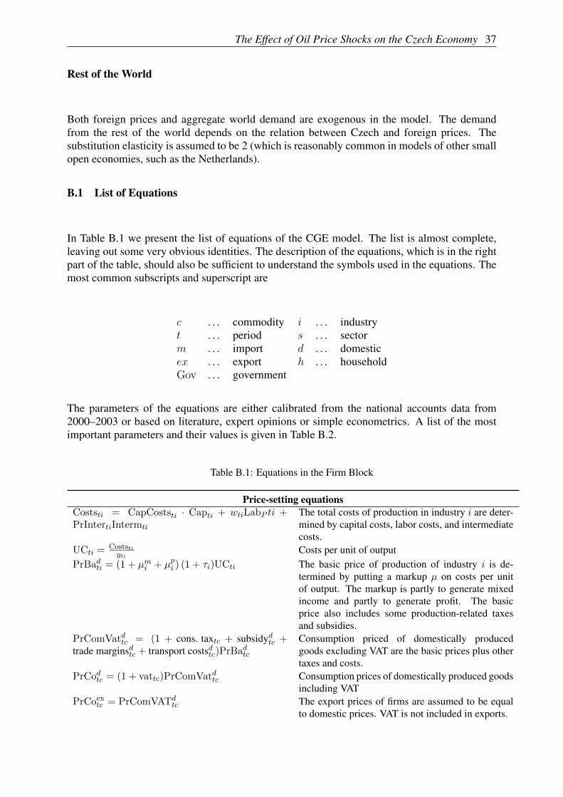
The Effect of Oil Price Shocks on the Czech Economy 37
Rest of the World
Both foreign prices and aggregate world demand are exogenous in the model. The demandfrom the rest of the world depends on the relation between Czech and foreign prices. Thesubstitution elasticity is assumed to be 2 (which is reasonably common in models of other smallopen economies, such as the Netherlands).
B.1 List of Equations
In Table B.1 we present the list of equations of the CGE model. The list is almost complete,leaving out some very obvious identities. The description of the equations, which is in the rightpart of the table, should also be sufficient to understand the symbols used in the equations. Themost common subscripts and superscript are
c . . . commodity i . . . industryt . . . period s . . . sectorm . . . import d . . . domesticex . . . export h . . . householdGov . . . government
The parameters of the equations are either calibrated from the national accounts data from2000–2003 or based on literature, expert opinions or simple econometrics. A list of the mostimportant parameters and their values is given in Table B.2.
Table B.1: Equations in the Firm Block
Price-setting equationsCoststi = CapCoststi · Capti + wtiLabP ti +PrIntertiIntermti
The total costs of production in industry i are deter-mined by capital costs, labor costs, and intermediatecosts.
UCti = Coststiyti
Costs per unit of outputPrBadti = (1 + µmi + µpi ) (1 + τi)UCti The basic price of production of industry i is de-
termined by putting a markup µ on costs per unitof output. The markup is partly to generate mixedincome and partly to generate profit. The basicprice also includes some production-related taxesand subsidies.
PrComVatdtc = (1 + cons. taxtc + subsidydtc +trade marginsdtc + transport costsdtc)PrBadtc
Consumption priced of domestically producedgoods excluding VAT are the basic prices plus othertaxes and costs.
PrCodtc = (1 + vattc)PrComVatdtc Consumption prices of domestically produced goodsincluding VAT
PrCoextc = PrComVATd
tc The export prices of firms are assumed to be equalto domestic prices. VAT is not included in exports.
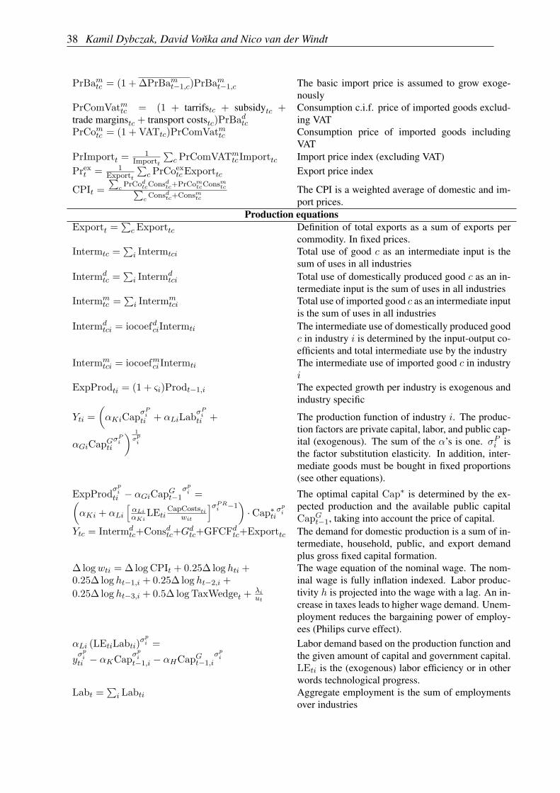
38 Kamil Dybczak, David Vonka and Nico van der Windt
PrBamtc = (1 + ∆PrBamt−1,c)PrBamt−1,c The basic import price is assumed to grow exoge-nously
PrComVatmtc = (1 + tarrifstc + subsidytc +trade marginstc + transport coststc)PrBadtc
Consumption c.i.f. price of imported goods exclud-ing VAT
PrComtc = (1 + VATtc)PrComVatmtc Consumption price of imported goods includingVAT
PrImportt = 1Importt
∑c PrComVATm
tc Importtc Import price index (excluding VAT)Prext = 1
Exportt
∑c PrCoex
tcExporttc Export price index
CPIt =∑
cPrCodtcConsdtc+PrComtcConsmtc∑
cConsdtc+Consmtc
The CPI is a weighted average of domestic and im-port prices.
Production equationsExportt =
∑c Exporttc Definition of total exports as a sum of exports per
commodity. In fixed prices.Intermtc =
∑i Intermtci Total use of good c as an intermediate input is the
sum of uses in all industriesIntermd
tc =∑i Intermd
tci Total use of domestically produced good c as an in-termediate input is the sum of uses in all industries
Intermmtc =
∑i Intermm
tci Total use of imported good c as an intermediate inputis the sum of uses in all industries
Intermdtci = iocoefdciIntermti The intermediate use of domestically produced good
c in industry i is determined by the input-output co-efficients and total intermediate use by the industry
Intermmtci = iocoefmci Intermti The intermediate use of imported good c in industry
iExpProdti = (1 + ςi)Prodt−1,i The expected growth per industry is exogenous and
industry specific
Yti =(αKiCapσ
Piti + αLiLabσ
Piti +
αGiCapGtiσPi
) 1
σpi
The production function of industry i. The produc-tion factors are private capital, labor, and public cap-ital (exogenous). The sum of the α’s is one. σPi isthe factor substitution elasticity. In addition, inter-mediate goods must be bought in fixed proportions(see other equations).
ExpProdσpiti − αGiCapGt−1
σpi =(αKi + αLi
[αLiαKi
LEtiCapCoststi
wit
]σPRi −1)·Cap∗ti
σpi
The optimal capital Cap∗ is determined by the ex-pected production and the available public capitalCapGt−1, taking into account the price of capital.
Ytc = Intermdtc+Consdtc+G
dtc+GFCFdtc+Exporttc The demand for domestic production is a sum of in-
termediate, household, public, and export demandplus gross fixed capital formation.
∆ logwti = ∆ log CPIt + 0.25∆ log hti +0.25∆ log ht−1,i + 0.25∆ log ht−2,i +0.25∆ log ht−3,i + 0.5∆ log TaxWedget + λi
ut
The wage equation of the nominal wage. The nom-inal wage is fully inflation indexed. Labor produc-tivity h is projected into the wage with a lag. An in-crease in taxes leads to higher wage demand. Unem-ployment reduces the bargaining power of employ-ees (Philips curve effect).
αLi (LEtiLabti)σpi =
yσpiti − αKCapσ
pit−1,i − αHCapGt−1,i
σpi
Labor demand based on the production function andthe given amount of capital and government capital.LEti is the (exogenous) labor efficiency or in otherwords technological progress.
Labt =∑i Labti Aggregate employment is the sum of employments
over industries

The Effect of Oil Price Shocks on the Czech Economy 39
NetProfitti = PrBadtiyti(1+τi)
− Coststi −Mixedti Net profit is determined as the value of productionin basic prices minus production taxes, costs, andmixed income.
GDPti = yti − Intermti Real value added per industry.hti = GDPti
LabtiLabor productivity in industry i
GDPt =∑i GDPti GDP is a sum of value added per industry in fixed
pricesInvestment, capital, and depreciation
Deprtsi = δisKt−1,s,i The depreciation in all industries is driven by a perindustry and sector depreciation coefficient, whichis calibrated from the data of the base year
Deprprivt = Deprt,Firms,i + Deprt,Households,i Depreciation in the private sector, which consists of
the firm and household sectors.Deptti =
∑s Deprtsi Depreciation per industry, aggregated over sectors
InvestPrivti = εi
(CAP∗ti − CAPti − InvestGov
ti
)Private net investment per industry. The investmentdepends on the difference between the optimal capi-tal and the available capital (taking into account thebehavior of the government)
InvestFirmsti = InvestPriv
ti All private net investment is assumed to be made byenterprises. Households’ capital (very small) there-fore remains constant.
Investti = InvestPrivti + InvestGov
ti The net investment per industry is a sum of privateand government investment
GrossInvtsi = Investtsi + Deprtsi Gross investment is a sum of net investment and de-preciation
GrossInvti = Investti + Deprti Gross investment is a sum of net investment and de-preciation
GrossInvt =∑i GrossInvti The aggregate (gross) investment is the sum of in-
vestment in all industriesPrmVATCap
ti
∑c InvMatrixci[
αcPrComVATd
tc+ 1−αc
PrComVATmtc
]= 1
The price of capital in sectors that do not pay VAT(enterprises, foreign)
PrVATCapti
∑c InvMatrixci[
αcPrCod
tc+ 1−αc
PrComtc
]= 1
The price of capital in sectors that do pay VAT
CapCoststi = PrCapti (δi + IRt) Capital costs are determined by depreciation and in-
terest rates and the price of capital goods.Capti = Capt−1,i + Investti The capital stock is equal to the capital stock in the
previous period plus net investmentThe household block
UH(Const) =∏Cc=1(Constc − Constc)shC0c The utility of households is based on consumption of
different types of goods i. The minimum consump-tion is Consi. The weight of i in the consumptionbasket is shC0i.
Constc = shMinConsc · Const−1,c The minimum consumption level of good c in agiven year is a fixed share of its actual consumptionlevel in the previous year
ConsExpt =∑c PrCotcConstc The minimum consumption expenditure of house-
holds

40 Kamil Dybczak, David Vonka and Nico van der Windt
NetHHIncomet = NetProfitt + MixedIncomet +WageBillt + InterestIncomet − SocContribt −IncomeTaxt + SocBent + OtTranst
Net household income is the sum of income fromshares, being self-employed, wages, interest minussocial contributions and taxes, plus social benefitsand other transfers
NetHHLendingt =shSAV
(NetHHIncomet − ConsExpt
) Net savings of households are a fixed share of theirnet income after minimum consumption
ConsExpt = NetHHIncomet −NetHHLendingt Consumption expenditure is the difference betweennet income and savings.
Constc = Constc + shC0cConsExpt−ConsExpt
PrCotcThe consumption demand for good c is determinedby the minimum consumption, the available incomeafter minimum consumption needs, and the price ofthe good.
ConsdtcConsmtc
=(
αhc1−αhc
) 1
1+σhc ·(
PrComtcPrCodtc
) 11+σc
h The distribution of consumption between domesticand imported goods depends on the ratio of domesticand import prices and the elasticities of consumerdemand.
Constc =(αhcCons
σchtc,d + (1− αhc )Cons
σchtc,m
) 1σch The total consumption of good c is a CES aggregate
of domestic and imported goodsut = LS−Labt
LSThe unemployment rate is the gap between the ex-ogenous labour supply and endogenous labour de-mand
Government expenditureGovContc,d = (1 + ∆GDP)GovCont−1,c,d The domestic consumption of the government grows
with GDPGovContc,m = (1 + ∆GDP)GovCont−1,c,m Imports for the government grow with GDPInvestGov
ti = exogenoust Government net investment per industry is assumedto be exogenous
Subst = −∑c subsidyc,dPrCotc,dytc +
subsidytc,mPrBatc,mImporttcThe subsidies on products are determined by thevalue of production and imports and exogenouscommodity-specific subsidy rates, which reflect thesituation in the base year
GovExpt = Subst + GovCont + InvestGovt +
OtTransGovt + InterestPayGov
t
The total expenditure of the government
CapGovit = (1− δGov
K )CapGovi,t−1 + InvestGov
ti The capital of the government (infrastructure) isused in the enterprises’ production function.
Government incomeVATt =
∑c vattc,dPrBatc,d(GovContc,d +
Consdtc)+vattc,mPrBatc,m(GovContc,m+Consmtc)The VAT collected. VAT rates are goods-specific,levied only on final consumption of households andthe government.
TARt =∑c tarrifstcPrBatc,mImporttc Collection of tarrifs
GovInct = NetProfitGovt + VATt + TARt +
IncomeTaxt + SocContribtThe composition of government income
Budget balanceNetLendingGov
t = GovInct −GovExpt The net lending of the governmentExport/Import equations
Exporttc = $cFDtc
(PrmtcPretc
)σec The export demand from abroad is determined by anexogenous trend FD and the ratio of export pricesto world prices. σec is the price elasticity of exports.

The Effect of Oil Price Shocks on the Czech Economy 41
Importtc = Intermmtc + Consmtc +Gmtc + GFCFmtc The demand for imported goods is a sum of inter-
mediate, household, and public demand plus grossfixed capital formation.
FDtc = (1 + ∆FDc)FDt−1,c The autonomous foreign demand for Czech goodsincreases exogenously by ∆FDc % a year.
CAt =∑c PrCoetcExporttc − PrBamtc Importtc The current account balance is defined as the differ-
ence between the value of exports and the value ofimports
Table B.2: The Key Parameters of the Model
Parameter Description Typical value
µi The profit margins firms put on top of theunit costs of production
0.08
τi The subsidy/tax on production of industryi
±0.03
cons.taxdtc The consumption tax on good c 0.075 in food0.090 in chemicals
trademarginsdtc The wholesale and retail margins on do-mestically produced goods
0.03–0.1
subsidydtc Subsidies on domestically produced com-modities
0.014 on food0.04 on transport
ςi Expected production growth, the techno-logical growth of the economy
3 % p.a.
FDtc Expected foreign demand growth 3 % p.a.σip The elasticity of substitution between pro-
duction factors0.5
— The capital:labor:infrastructure ratio in theproduction function
0.3:0.6:0.1
λi The Phillips curve effect, the impact of un-employment on wages
0.01
δi Depreciation of physical capital 0.06σεc The price elasticity of exports 1.7σhc The price elasticity of imports for final
consumption2

CNB WORKING PAPER SERIES 5/2008 Kamil Dybczak
David Voňka Nico van der Windt
The effect of oil price shocks on the Czech economy
4/2008 Magdalena M. Borys Roman Horváth
The effects of monetary policy in the Czech Republic: An empirical study
3/2008 Martin Cincibuch Tomáš Holub Jaromír Hurník
Central bank losses and economic convergence
2/2008 Jiří Podpiera Policy rate decisions and unbiased parameter estimation in conventionally estimated monetary policy rules
1/2008
Balázs Égert Doubravko Mihaljek
Determinants of house prices in Central and Eastern Europe
17/2007 Pedro Portugal U.S. unemployment duration: Has long become bonger or short become shorter?
16/2007 Yuliya Rychalovská Welfare-based optimal monetary policy in a two-sector small open economy
15/2007 Juraj Antal František Brázdik
The effects of anticipated future change in the monetary policy regime
14/2007 Aleš Bulíř Kateřina Šmídková Viktor Kotlán David Navrátil
Inflation targeting and communication: Should the public read inflation reports or tea leaves?
13/2007 Martin Cinncibuch Martina Horníková
Measuring the financial markets' perception of EMU enlargement: The role of ambiguity aversion
12/2007 Oxana Babetskaia-Kukharchuk
Transmission of exchange rate shocks into domestic inflation: The case of the Czech Republic
11/2007 Jan Filáček Why and how to assess inflation target fulfilment 10/2007 Michal Franta
Branislav Saxa Kateřina Šmídková
Inflation persistence in new EU member states: Is it different than in the Euro area members?
9/2007 Kamil Galuščák Jan Pavel
Unemployment and inactivity traps in the Czech Republic: Incentive effects of policies
8/2007 Adam Geršl Ieva Rubene Tina Zumer
Foreign direct investment and productivity spillovers: Updated evidence from Central and Eastern Europe
7/2007 Ian Babetskii Luboš Komárek Zlatuše Komárková
Financial integration of stock markets among new EU member states and the euro area
6/2007 Anca Pruteanu-Podpiera Laurent Weill Franziska Schobert
Market power and efficiency in the Czech banking sector
5/2007 Jiří Podpiera Laurent Weill
Bad luck or bad management? Emerging banking market experience
4/2007 Roman Horváth The time-varying policy neutral rate in real time: A predictor for future inflation?

3/2007 Jan Brůha Jiří Podpiera Stanislav Polák
The convergence of a transition economy: The case of the Czech Republic
2/2007 Ian Babetskii Nauro F. Campos
Does reform work? An econometric examination of the reform-growth puzzle
1/2007 Ian Babetskii Fabrizio Coricelli Roman Horváth
Measuring and explaining inflation persistence: Disaggregate evidence on the Czech Republic
13/2006 Frederic S. Mishkin Klaus Schmidt-Hebbel
Does inflation targeting make a difference?
12/2006 Richard Disney Sarah Bridges John Gathergood
Housing wealth and household indebtedness: Is there a household ‘financial accelerator’?
11/2006 Michel Juillard Ondřej Kameník Michael Kumhof Douglas Laxton
Measures of potential output from an estimated DSGE model of the United States
10/2006 Jiří Podpiera Marie Raková
Degree of competition and export-production relative prices when the exchange rate changes: Evidence from a panel of Czech exporting companies
9/2006 Alexis Derviz Jiří Podpiera
Cross-border lending contagion in multinational banks
8/2006 Aleš Bulíř Jaromír Hurník
The Maastricht inflation criterion: “Saints” and “Sinners”
7/2006 Alena Bičáková Jiří Slačálek Michal Slavík
Fiscal implications of personal tax adjustments in the Czech Republic
6/2006 Martin Fukač Adrian Pagan
Issues in adopting DSGE models for use in the policy process
5/2006 Martin Fukač New Keynesian model dynamics under heterogeneous expectations and adaptive learning
4/2006 Kamil Dybczak Vladislav Flek Dana Hájková Jaromír Hurník
Supply-side performance and structure in the Czech Republic (1995–2005)
3/2006 Aleš Krejdl Fiscal sustainability – definition, indicators and assessment of Czech public finance sustainability
2/2006 Kamil Dybczak Generational accounts in the Czech Republic 1/2006 Ian Babetskii Aggregate wage flexibility in selected new EU member states
14/2005 Stephen G. Cecchetti The brave new world of central banking: The policy challenges posed by asset price booms and busts
13/2005 Robert F. Engle Jose Gonzalo Rangel
The spline GARCH model for unconditional volatility and its global macroeconomic causes
12/2005 Jaromír Beneš Tibor Hlédik Michael Kumhof David Vávra
An economy in transition and DSGE: What the Czech national bank’s new projection model needs

11/2005 Marek Hlaváček Michael Koňák Josef Čada
The application of structured feedforward neural networks to the modelling of daily series of currency in circulation
10/2005 Ondřej Kameník Solving SDGE models: A new algorithm for the sylvester equation 9/2005 Roman Šustek Plant-level nonconvexities and the monetary transmission
mechanism 8/2005 Roman Horváth Exchange rate variability, pressures and optimum currency
area criteria: Implications for the central and eastern european countries
7/2005 Balázs Égert Luboš Komárek
Foreign exchange interventions and interest rate policy in the Czech Republic: Hand in glove?
6/2005 Anca Podpiera Jiří Podpiera
Deteriorating cost efficiency in commercial banks signals an increasing risk of failure
5/2005 Luboš Komárek Martin Melecký
The behavioural equilibrium exchange rate of the Czech koruna
4/2005 Kateřina Arnoštová Jaromír Hurník
The monetary transmission mechanism in the Czech Republic (evidence from VAR analysis)
3/2005 Vladimír Benáček Jiří Podpiera Ladislav Prokop
Determining factors of Czech foreign trade: A cross-section time series perspective
2/2005 Kamil Galuščák Daniel Münich
Structural and cyclical unemployment: What can we derive from the matching function?
1/2005 Ivan Babouček Martin Jančar
Effects of macroeconomic shocks to the quality of the aggregate loan portfolio
10/2004 Aleš Bulíř Kateřina Šmídková
Exchange rates in the new EU accession countries: What have we learned from the forerunners
9/2004 Martin Cincibuch Jiří Podpiera
Beyond Balassa-Samuelson: Real appreciation in tradables in transition countries
8/2004 Jaromír Beneš David Vávra
Eigenvalue decomposition of time series with application to the Czech business cycle
7/2004 Vladislav Flek, ed. Anatomy of the Czech labour market: From over-employment to under-employment in ten years?
6/2004 Narcisa Kadlčáková Joerg Keplinger
Credit risk and bank lending in the Czech Republic
5/2004 Petr Král Identification and measurement of relationships concerning inflow of FDI: The case of the Czech Republic
4/2004 Jiří Podpiera Consumers, consumer prices and the Czech business cycle identification
3/2004 Anca Pruteanu The role of banks in the Czech monetary policy transmission mechanism
2/2004 Ian Babetskii EU enlargement and endogeneity of some OCA criteria: Evidence from the CEECs
1/2004 Alexis Derviz Jiří Podpiera
Predicting bank CAMELS and S&P ratings: The case of the Czech Republic

CNB RESEARCH AND POLICY NOTES
2/2007 Carl E. Walsh Inflation targeting and the role of real objectives 1/2007 Vojtěch Benda
Luboš Růžička Short-term forecasting methods based on the LEI approach: The case of the Czech Republic
2/2006 Garry J. Schinasi Private finance and public policy 1/2006 Ondřej Schneider The EU budget dispute – A blessing in disguise?
5/2005 Jan Stráský Optimal forward-looking policy rules in the quarterly projection model of the Czech National Bank
4/2005 Vít Bárta Fulfilment of the Maastricht inflation criterion by the Czech Republic: Potential costs and policy options
3/2005 Helena Sůvová Eva Kozelková David Zeman Jaroslava Bauerová
Eligibility of external credit assessment institutions
2/2005 Martin Čihák Jaroslav Heřmánek
Stress testing the Czech banking system: Where are we? Where are we going?
1/2005 David Navrátil Viktor Kotlán
The CNB’s policy decisions – Are they priced in by the markets?
4/2004 Aleš Bulíř External and fiscal sustainability of the Czech economy: A quick look through the IMF’s night-vision goggles
3/2004 Martin Čihák Designing stress tests for the Czech banking system 2/2004 Martin Čihák Stress testing: A review of key concepts 1/2004 Tomáš Holub Foreign exchange interventions under inflation targeting:
The Czech experience
CNB ECONOMIC RESEARCH BULLETIN
November 2008 Inflation Targeting and DSGE Models April 2008 Ten years of inflation targeting December 2007 Fiscal policy and its sustainability August 2007 Financial stability in a transforming economy November 2006 ERM II and euro adoption August 2006 Research priorities and central banks November 2005 Financial stability May 2005 Potential output October 2004 Fiscal issues May 2004 Inflation targeting December 2003 Equilibrium exchange rate

Czech National Bank Economic Research Department Na Příkopě 28, 115 03 Praha 1
Czech Republic phone: +420 2 244 12 321
fax: +420 2 244 14 278 http://www.cnb.cz
e-mail: [email protected] ISSN 1803-7070