Working Paper No. 494

Fiscal Policy in a Stock-Flow Consistent (SFC) Model

by

Wynne Godley and Marc Lavoie*

April 2007

*The authors are, respectively, Emeritus Professor of Applied Economics of CambridgeUniversity (and Emeritus Fellow of King’s College) and Professor of Economics at theUniversity of Ottawa. We wish to thank Ken Coutts, Peter Docherty, and EkkehartSchlicht for their comments.

The Levy Economics Institute Working Paper Collection presents research in progress byLevy Institute scholars and conference participants. The purpose of the series is to

disseminate ideas to and elicit comments from academics and professionals.

The Levy Economics Institute of Bard College, founded in 1986, is a nonprofit,nonpartisan, independently funded research organization devoted to public service.Through scholarship and economic research it generates viable, effective public policyresponses to important economic problems that profoundly affect the quality of life inthe United States and abroad.

The Levy Economics InstituteP.O. Box 5000

Annandale-on-Hudson, NY 12504-5000http://www.levy.org

Copyright © The Levy Economics Institute 2007 All rights reserved.

2

ABSTRACT

This paper deploys a simple stock-flow consistent (SFC) model in order to examine

various contentions regarding fiscal and monetary policy. It follows from the model

that if the fiscal stance is not set in the appropriate fashion that is, at a well-defined

level and growth rate—then full employment and low inflation will not be achieved in

a sustainable way. We also show that fiscal policy on its own could achieve both full

employment and a target rate of inflation. Finally, we arrive at two unconventional

conclusions: first, that an economy (described within an SFC framework) with a real

rate of interest net of taxes that exceeds the real growth rate will not generate

explosive interest flows, even when the government is not targeting primary

surpluses; and, second, that it cannot be assumed that a debtor country requires a trade

surplus if interest payments on debt are not to explode.

Keywords: Stock-Flow Consistency, Fiscal Policy, Public Debt, New Consensus on

Monetary Economics, Current Account Deficit

JEL Classifications: E120, E620, F410

3

In our book, Monetary Economics (Godley and Lavoie 2007), we claimed that a

particular level of government expenditure relative to tax rates, and also relative to

GDP, is essential if stable, noninflationary growth and full employment are to be

achieved. We argued, on the basis of simulation models, that monetary policy on its

own was unable to maintain full employment and low inflation for more than a short

period of time, unless fiscal policy was appropriate. Our conclusions conflict with

those of the “New Consensus,” which holds that a correct setting of interest rates is

the necessary and sufficient condition for achieving noninflationary growth at full

employment, leaving fiscal policy rather in the air. This has led different countries to

adopt various different targets for the nominal budget deficit and government debt as

proportions of (nominal) GDP measured ex post. 1 But the rationale for such targets

has never been clear (at least to us).

In this paper, we shall deploy a simple stock-flow consistent (SFC) model

which will enable us to outline the way in which the fiscal stance (as defined below)

should be determined as the necessary, though not always sufficient, condition for the

achievement of the major objectives of macroeconomic policy. We shall also show

that the new emphasis on monetary policy may be quite misplaced. In theory

(although in practice this may be an entirely different issue), fiscal policy can achieve

everything the central banks claim they are able to do through monetary policy. In

other words, just as the success of monetary policy is judged on the basis of medium-

term achievements, and not in the monthly or quarterly variations of the inflation rate,

there is a similar role to be played by fiscal policy on the medium-term evolution of

output and employment.

Our paper is made up of three sections. In the first section, we present a highly

simplified closed economy SFC model, in which it is shown that a full (growing)

steady state with full employment can only be achieved if the fiscal policy setting is

appropriate. In the second section, we extend our SFC model by endogenizing the

inflation rate through a vertical Phillips curve, as can be found in the New Consensus

equations. We then assume a budget policy reaction function, similar to the central

bank reaction function of the New Consensus, whereby the government achieves both

full employment and target inflation rates whenever the economy is subjected to

shocks or changes in the values of the behavioral parameters. Finally, in the third 1 Obvious examples are the Maastricht rules in the European Union, Gordon Brown’s “Golden” rule in the United Kingdom, and various rules forbidding or attempting to forbid government deficits.

4

section, we add a very rudimentary foreign sector, still keeping the SFC features of

our model, to arrive at results that are somewhat surprising.

A SIMPLE SFC GROWTH ECONOMY MODEL

An Outline of the SFC Model

The following matrix describes the accounting structure of the basic model we shall

use. All variables in this matrix are measured at current prices. The counterpart real

variables will be defined in the text which follows. As always in a transactions-flow

matrix, each row and each column must sum to zero.

TABLE 1: Transactions-flow matrix of a simple closed-economy model Households Firms Government Sum

Private Expenditures

- X + X 0

Government Expenditures

+ G -G 0

Income (GDP) +Y -Y 0 Taxes -T +T 0

Interest + r.GD-1 - r.GD-1 0 Change in

wealth/Debt - ∆V +∆GD 0

Sum 0 0 0 0

All variables are defined in the matrix apart from r (the nominal interest rate),

V (private wealth), and GD (government debt). For simplification, the accumulation

of capital by firms has been assumed away.

In what follows, the numbered equations correspond with those directly

entering the model (i.e., those required by the computer to obtain a solution).

Equations introduced using capital letters (A, B, etc.) are auxiliaries which hopefully

aid the exposition. While the model is very simple, its exposition is slightly intricate

because decisions by the private sector are assumed to be taken entirely in real terms,

while those of the government regarding interest rates and tax rates together with

targets for budget balances are measured in nominal terms.

5

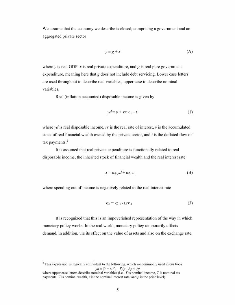
We assume that the economy we describe is closed, comprising a government and an

aggregated private sector

y ≡ g + x (A)

where y is real GDP, x is real private expenditure, and g is real pure government

expenditure, meaning here that g does not include debt servicing. Lower case letters

are used throughout to describe real variables, upper case to describe nominal

variables.

Real (inflation accounted) disposable income is given by

yd ≡ y + rr.v-1 – t (1)

where yd is real disposable income, rr is the real rate of interest, v is the accumulated

stock of real financial wealth owned by the private sector, and t is the deflated flow of

tax payments.2

It is assumed that real private expenditure is functionally related to real

disposable income, the inherited stock of financial wealth and the real interest rate

x = α1.yd + α2.v-1 (B)

where spending out of income is negatively related to the real interest rate

α1 = α10 - ι.rr-1 (3)

It is recognized that this is an impoverished representation of the way in which

monetary policy works. In the real world, monetary policy temporarily affects

demand, in addition, via its effect on the value of assets and also on the exchange rate.

2 This expression is logically equivalent to the following, which we commonly used in our book

yd ≡ (Y + r.V-1 - T)/p - ∆p.v-1/p where upper case letters describe nominal variables (i.e., Y is nominal income, T is nominal tax payments, V is nominal wealth, r is the nominal interest rate, and p is the price level).

6

As the change in the real stock of wealth is equal by definition to real

disposable income less expenditure, that is, in line with the Haig-Simons definition of

real disposable income,

∆v ≡ yd – x [≡ real private saving] (C)

equation (B) can equivalently be written as a wealth adjustment function

v = v-1 + α2.(v* - v-1) (4)

This implies that the desired real stock of financial wealth, v*, is a determinate

proportion of disposable income

v* = α3..yd (5)

where

α3 ≡ (1 - α1)/ α2 (2)

As we are going to make suggestions about policy in the real world, it is

important to note here that the coefficient α3 is intended to refer to a long-run

tendency. In the short run the ratio of desired financial wealth to disposable income

will fluctuate, for instance, because of capital gains and losses and also credit cycles.

It is precisely from such (normally) short-term influences that we wish to abstract,

since there will only be rare occasions on which it will be appropriate to use fiscal

policy to offset them.

It follows that private expenditure enters the equation system in the form

x ≡ yd - ∆v (7)

since yd and v are already determined in (1) and (4).

Nominal taxes, T, are raised as a proportion, θ, of nominal private factor

income, Y, plus nominal interest receipts.

7

T = θ.(Y + r.V-1) (8)

where Y is nominal GDP, V is the nominal stock of financial wealth, and r is the

nominal interest rate

Y ≡ y.p (9)

and

V ≡ v.p (10)

where p is the price level.

Nominal and real interest rates are related according to the Fisher formula

rr ≡ (1 + r)/(1 + π) -1 (11)

where π, is defined as the rate of price inflation, which is a given in our little model

π ≡ ∆p/p-1 (12)

The economy is assumed to grow at a rate, gr, and to be at a level which

corresponds with full employment, as well as low and stable inflation. In the wording

of mainstream economics, the output gap is zero at all times and the economy is at the

NAIRU. We don’t actually believe that such conditions usually occur, or that the

NAIRU is a useful concept, but we set out these conditions for the sake of discussion.

Another way to understand equation (13) below is to say that, although the economy

may not be performing at full employment at all time, we are trying to ascertain, as

will be clear later, the fiscal stance that needs to be adopted, if the economy is to be at

full employment on average.

y = y-1.(1 + gr) (13)

8

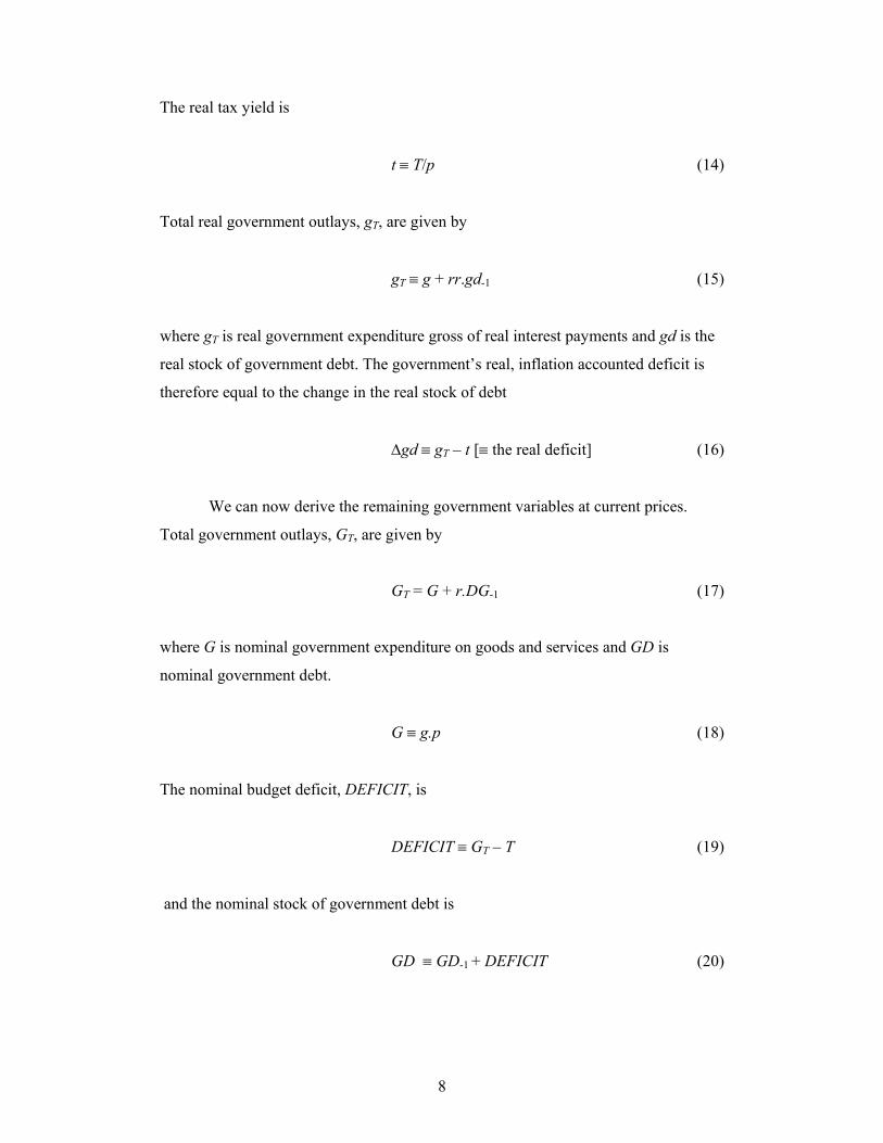
The real tax yield is

t ≡ T/p (14)

Total real government outlays, gT, are given by

gT ≡ g + rr.gd-1 (15)

where gT is real government expenditure gross of real interest payments and gd is the

real stock of government debt. The government’s real, inflation accounted deficit is

therefore equal to the change in the real stock of debt

∆gd ≡ gT – t [≡ the real deficit] (16)

We can now derive the remaining government variables at current prices.

Total government outlays, GT, are given by

GT = G + r.DG-1 (17)

where G is nominal government expenditure on goods and services and GD is

nominal government debt.

G ≡ g.p (18)

The nominal budget deficit, DEFICIT, is

DEFICIT ≡ GT – T (19)

and the nominal stock of government debt is

GD ≡ GD-1 + DEFICIT (20)

9

To complete the model we now only have to invert equation (A), thereby

making the real flow of government expenditure on goods and services endogenous.

g ≡ y - x (21)

In other words, we assume that, for a given tax rate, pure government

expenditures take up any slack that could exist between potential (or full-

employment) output and private expenditures. We have recently become aware that a

paper by Ekkehart Schlicht (2006) shows a remarkable degree of affinity with the

present work, both in its modeling strategy and in its conclusions.

Our model is now complete in the sense that it can be solved for the level

and growth of government expenditure and the budget deficit conditional on any

configuration of assumptions regarding r and θ—the policy variables—as well as gr,

α10, α2, ι, and π.

Note finally that nominal private saving, or the net accumulation of financial

assets, is given by

NAFA ≡ (Y + r.V-1 – T) – X (22)

This identity will provide a useful check that the accounting of the model is

correct since nominal private saving should be found to be equal to the (nominal)

budget deficit (DEFICIT) although there is no (individual) equation to make this

happen.3

Some Arithmetical Results

In this first section we confine ourselves to solutions which describe growing steady

states, in which all real stocks and flows are growing at the same rate while all

nominal stocks and flows are growing at a different, higher rate. We first set forth a

base run in which real output and all other real flows and stocks grow at 2.5% per

annum, thus assuming that this is known to be the rate at which the productive

potential of the economy is growing. In addition, we make arbitrary but

uncontroversial assumptions about the tax rate (25%), the inflation rate (2%), the 3 In the wording of our book, as can be read from the one before last row of Table 1, the redundant equation is: DEFICIT ≡ NAFA

10

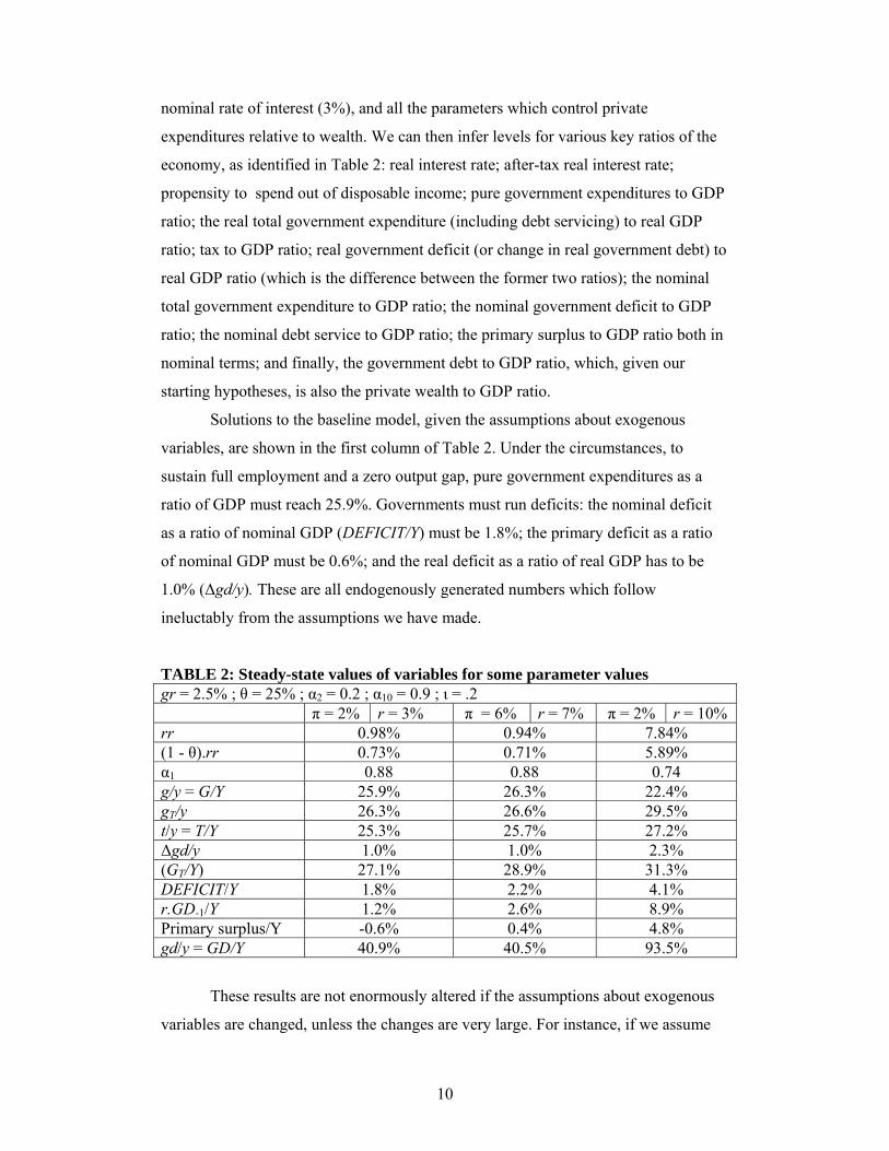
nominal rate of interest (3%), and all the parameters which control private

expenditures relative to wealth. We can then infer levels for various key ratios of the

economy, as identified in Table 2: real interest rate; after-tax real interest rate;

propensity to spend out of disposable income; pure government expenditures to GDP

ratio; the real total government expenditure (including debt servicing) to real GDP

ratio; tax to GDP ratio; real government deficit (or change in real government debt) to

real GDP ratio (which is the difference between the former two ratios); the nominal

total government expenditure to GDP ratio; the nominal government deficit to GDP

ratio; the nominal debt service to GDP ratio; the primary surplus to GDP ratio both in

nominal terms; and finally, the government debt to GDP ratio, which, given our

starting hypotheses, is also the private wealth to GDP ratio.

Solutions to the baseline model, given the assumptions about exogenous

variables, are shown in the first column of Table 2. Under the circumstances, to

sustain full employment and a zero output gap, pure government expenditures as a

ratio of GDP must reach 25.9%. Governments must run deficits: the nominal deficit

as a ratio of nominal GDP (DEFICIT/Y) must be 1.8%; the primary deficit as a ratio

of nominal GDP must be 0.6%; and the real deficit as a ratio of real GDP has to be

1.0% (∆gd/y). These are all endogenously generated numbers which follow

ineluctably from the assumptions we have made.

TABLE 2: Steady-state values of variables for some parameter values gr = 2.5% ; θ = 25% ; α2 = 0.2 ; α10 = 0.9 ; ι = .2 π = 2% r = 3% π = 6% r = 7% π = 2% r = 10% rr 0.98% 0.94% 7.84% (1 - θ).rr 0.73% 0.71% 5.89% α1 0.88 0.88 0.74 g/y = G/Y 25.9% 26.3% 22.4% gT/y 26.3% 26.6% 29.5% t/y = T/Y 25.3% 25.7% 27.2% ∆gd/y 1.0% 1.0% 2.3% (GT/Y) 27.1% 28.9% 31.3% DEFICIT/Y 1.8% 2.2% 4.1% r.GD-1/Y 1.2% 2.6% 8.9% Primary surplus/Y -0.6% 0.4% 4.8% gd/y = GD/Y 40.9% 40.5% 93.5%

These results are not enormously altered if the assumptions about exogenous

variables are changed, unless the changes are very large. For instance, if we assume

11

an inflation rate of 6%, with a consequential increase of 4 percentage points in the

nominal interest rate, as r moves up from 3% to 7%—thus keeping the real interest

rate approximately constant—the ratio of pure government expenditures to GDP

barely moves, going from 25.9% to 26.3%. The real deficit to real GDP ratio does not

change, while the nominal deficit to GDP ratio moves up from 1.8 to 2.2%, with the

primary surplus going from a negative to a positive position. As to the debt to GDP

ratio, it also barely changes, going from 40.9% to 40.5%.

Some Analytical Results

Simple but tedious computations can help explain these results. We can derive the

following steady-state values for three of the main real ratios of our economy:

The government expenditure to GDP ratio:

})1(

)1/()1({)(*)(gr

rrgry

gdyg

+π+π+θ−−

+θ= (23)

The public debt to GDP ratio:

rrgrgr

ygd

)1()1()]1/()1[()1()1()1(*)(

112

1

θ−α−−π+πθα−+α++θ−α−

= (24)

The real deficit to real GDP ratio:

rrgrgr

ygd

)1()1()]1/()1[()1()1(*)(

112

1

θ−α−−π+πθα−+α+θ−α−

=∆ (25)

With no inflation (π = 0), and with the real rate of growth equal to the real rate of

interest net of tax (gr = (1 – θ)rr), these steady-state solutions get highly simplified:

θ=*)(y

gd (23’)

12

21

1 )1()1()1(*)(

α+α+θ−α−

=gr

gry

gd (24’)

)()1()1(*)(

21

1

ααθα

+−−

=gr

gry

gd (25’)

In this case, taking the derivative of equation (24’) with respect to gr, it is

rather obvious that an increase in the real rate of growth of the economy,

accompanied by an equal increase in the real rate of interest net of tax, will lead to a

decrease in the public debt to GDP ratio, as long as the propensity to spend out of

disposable income is higher than that out of wealth (α1 > α2).4 Only when the growth

rate of the economy gets down to nil—the stationary state—should the real deficit

become zero and the real budget be balanced.

Inspection of equation (24) also shows that, keeping all the other parameters

constant (including the real interest rate), an increase in the propensity to save out of

wealth (α2), in the tax rate (θ), and in the inflation rate (π) leads to a lower steady-state

public debt to GDP ratio, while an increase in the real rate of interest (rr) leads to a

higher steady-state debt to GDP ratio, as one would suspect.

A Surprising Result

Our simple SFC model can, however, provide us with a more surprising result. It is

usually asserted that for the debt dynamics to remain sustainable, the real rate of

interest must be lower than the real rate of growth of the economy for a given primary

budget surplus to GDP ratio. If this condition is not fulfilled, the government needs to

pursue a discretionary policy that aims to achieve a sufficiently large primary surplus.

We can easily demonstrate that there are no such requirements in a fully-consistent

stock-flow model such as ours. The last column of Table 2 shows what occurs if the

nominal rate of interest is pushed to 10%, thus raising the real rate of interest rr to

7.84%. Even if we reinterpret this condition as meaning that the real rate of interest

net of tax has to be smaller than the real rate of growth, as does Feldstein (1976), the

real rate of interest net of tax, 5.89%, is still way above the real rate of growth of the 4 This effect will be further enforced because an increase in rr leads to an induced fall in the propensity to spend out of disposable income, the α1 coefficient, according to equation (3).

13

economy which stands at 2.5%. An increase in the real interest rate induces, in our

fiscally-generated full-employment model, a substantial increment in the steady-state

public debt to GDP ratio and deficit to GDP ratio, as many of us would suspect. But

this process reaches a limit. The (real) primary surplus to GDP ratio does achieve a

positive figure in the steady state (here +4.8%), as traditional analysis would have it

when the rate of interest is larger than the rate of growth. But this is not achieved in

the model by the exogenous imposition of a large primary surplus. Instead, the only

behavioral requirement that has been imposed upon the public sector is a high enough

level of pure government expenditure, such that full employment output is verified in

each period.

The numbers in the last column of Table 2 were not obtained by relying on

the steady-state values of equations (24–26), although they correspond to these

equations. They were obtained by running our first model with a simulation program,

MODLER. Figure 1 illustrates the transition of our economy from the initial steady

state, with low real interest rates, towards the new steady state, with real interest rates

standing at 7.84%. Clearly, despite the overly high real interest rates, the real deficit

to real GDP ratio converges, and so does the public debt to GDP ratio. The model

yields stable, nonexplosive results.

FIGURE 1 Impact of an increase in the nominal interest rate, from 3% to 10%, on the real deficit to real GDP ratio and on the public debt to GDP ratio, when the real growth rate is still 2.5%

14

We have run further experiments, with real rates as high as 25%, and the

model still held up. The debt to GDP ratio would then rise to absurd numbers, at about

240%, but the real deficit to real GDP ratio, after spiking to above 30% for one

period, would be brought back to a steady ratio of about 7.5%.

Defining the government’s fiscal stance as the ratio of real government outlays

relative to the average tax rate (i.e., (g + rr.gd)/ θ), it follows from the model that not

only must the fiscal stance be set at a particular level at any point of time for full

employment to be achieved, but, once full employment has been achieved, the fiscal

stance must grow (by 2.5% per annum) through time, as long as the real rate of

growth in productive potential remain at 2.5%.

It also follows clearly from Figure 1 that if central banks, for whatever reason,

have decided to kick real interest rates up, there will be definite repercussions on the

deficit to GDP ratio and on the public debt to GDP ratio, even if full employment is

preserved at all times through an appropriate choice of the fiscal stance. It makes no

sense to put limits on deficit or debt ratios, as in the Maastricht rules and Gordon

Brown’s golden rules, outside the context of how any economy actually works.

A FISCAL POLICY ALTERNATIVE TO THE NEW CONSENSUS ON

MONETARY POLICY

It has been pointed out by a variety of authors that the role of fiscal policy has been

considerably reduced over the last 20 years or so, prominence being given to

monetary policy to achieve both a target rate of inflation and a level of demand

compatible with potential output or full-employment output. Authors in the New

Consensus tradition have been particularly silent with regard to the role that fiscal

policy ought to play. As Philip Arestis and Malcolm Sawyer (2004) point out, “the

‘new consensus’ model (or equivalent) provides little role for fiscal policy.” This is

particularly puzzling, because, according to their survey of central bank empirical

results, any negative impact on the rate of inflation works through reductions in

aggregate demand, and these require very large changes in interest rates to be of any

significance. As a consequence, they conclude by saying that “fiscal policy remains a

potent tool for offsetting major changes in the level of aggregate demand” (Arestis

and Sawyer 2004). Here we wish to show that fiscal policy can, in principle, achieve

what New Consensus authors claim that monetary policy can achieve.

15

Some authors say that fiscal policy has been discredited as a short-term

regulator of aggregate demand because of its well-known logistical problems, such as

lags in legislation, implementation, and effects, as well as because of the politics

involved. While those concerns are certainly relevant and worth discussing, we do not

wish to address them at this stage, as we mainly attempt to make a series of

theoretical points. Suffice it to say for the moment that central bankers, now and ever

since the empirical works of Milton Friedman, recognize that monetary policy usually

takes from 12 to 24 months to impinge on inflation. There are bound to be lags as well

with fiscal policy, but fiscal policy has proven incredibly effective where it has been

used relentlessly, for instance in the case of the Reagan fiscal expansion in the 1980s

and the Bush fiscal expansion following 9/11.

If lags in the implementation of fiscal policy are to be reduced, there is clearly

a need for institutional change, whereby plans for government expenditures, in

particular government investment, would be prepared way in advance, ready to go

when required. Others, such as Randall Wray (1998) or Juniper and Mitchell (2005),

have argued in favor of public service employment programs that would kick off the

moment output demand falls behind full-employment output.

A Fiscal Policy Reaction Function

We start with the simple model that was presented in the previous section, adding two

behavioral equations. First, we now make the rate of price inflation endogenous, by

assuming that inflation reacts to the output gap, as it does in the much-acclaimed

vertical Phillips curve analysis first introduced by Milton Friedman. New Consensus

authors, as recalled by various Post-Keynesian economists in their critiques of the

New Consensus (Setterfield 2005; Lavoie 2006), usually assume some variant of the

vertical Phillips curve, which, in its most simplified form, can be presented as:

π = π-1 + ε + γ(y – ys)/y (26)

or

∆π = ε + γ(y – ys)/y

We assume here, although we have denied the relevance of this

accelerationist view of inflation on numerous occasions (e.g., Godley and Lavoie

2007), that the change in the rate of inflation depends on the output gap, as usually

16

defined by mainstream economists, and on some cost-side determinant, ε, which we

will detail no more. Thus, ys stands for potential output while y now stands for the

demand-led actual output, with γ measuring the sensitivity of inflation to the relative

output gap. As we said in the introduction, we introduce such a vertical Phillips curve

as a means of exploring the relevance of fiscal policy, in a world—with the

accelerationist theory of inflation—which is most favorable to mainstream economics.

If we can demonstrate that fiscal policy is of supreme relevance within that

framework, then a fortiori it should play a substantial role in a (Post-Keynesian) world

devoid of the accelerationist hypothesis.

Because we now clearly distinguish between potential output and actual

output, as determined by demand, we need to rewrite two equations of our simple

model. Equations (13) and (21), which for convenience we repeat here,

y = y-1.(1 + gr) (13)

g ≡ y - x (21)

get replaced by equations (13-2) and (21-2):

ys = ys-1.(1 + gr) (13-2)

y = g + x (21-2)

We thus need an additional equation that will explain real pure government

expenditures, g. In analogy with the reaction function of the central bank, which

determines the nominal or the real interest rate set by the central bank, we define a

fiscal reaction function, which defines the growth rate of real pure government

expenditures, calling grG this growth rate. We thus have the following two equations:

g = g-1 (1 + grG) (27)

grG = gr – β1.∆π-1 – β2.(π-1 – πT) (28)

The growth rate of real pure government expenditures, grG, is thus anchored

by the growth rate of potential output, gr. It is lower than gr when the lagged inflation

17

rate is rising and when the actual inflation rate is above the target inflation rate πT, a

target presumably set together by the central bank and the government. Because of

equation (26) and its accelerationist hypothesis, to say that the growth rate of real pure

government expenditures is lower when the rate of inflation rises implies that this

growth rate will tend to be lower when actual output overtakes potential output.

Obviously, this kind of fiscal policy mimics the various central bank

reaction functions that have been proposed since the 1990s. In particular, gr, the rate

of growth of potential output, or the natural rate of growth, plays a role that is similar

to that of the natural rate of interest in the New Consensus reaction function

equations. It is assumed that governments react to lagged inflation rates, rather than to

actual or expected inflation rates, on the realistic grounds that fiscal policy may have

a reaction time somewhat longer than monetary policy.

Experiments with the Fiscal Policy Reaction Function Model

We can conduct various experiments with our slightly more sophisticated SFC model.

As usual, we start from a baseline case, where steady-state positions have been

reached—with capacity, real output, and real government expenditures all growing at

2.5%, along with the real stocks of the economy. Inflation, as before, is assumed to

run at 2%. The nominal and real interest rates, as before, are set at 3% and nearly 1%.

Experiments have shown that the behavior of the model hardly changes whether

nominal or real interest rates are considered to be the exogenous variable. In the

figures that will be shown, it has been assumed that the central bank has given itself

as a policy to keep the real rate at a constant level, so that equation (11) needs to be

reversed into equation (11-2), which becomes the central bank reaction function:

r = rr + π + π.rr (11-2)

As a first experiment, let us assume that the central bank is unhappy with its

current inflation target, and has managed to successfully lobby the government into

accepting a lower inflation target, say πT = 1.5%. What will then happen? Figures 2 to

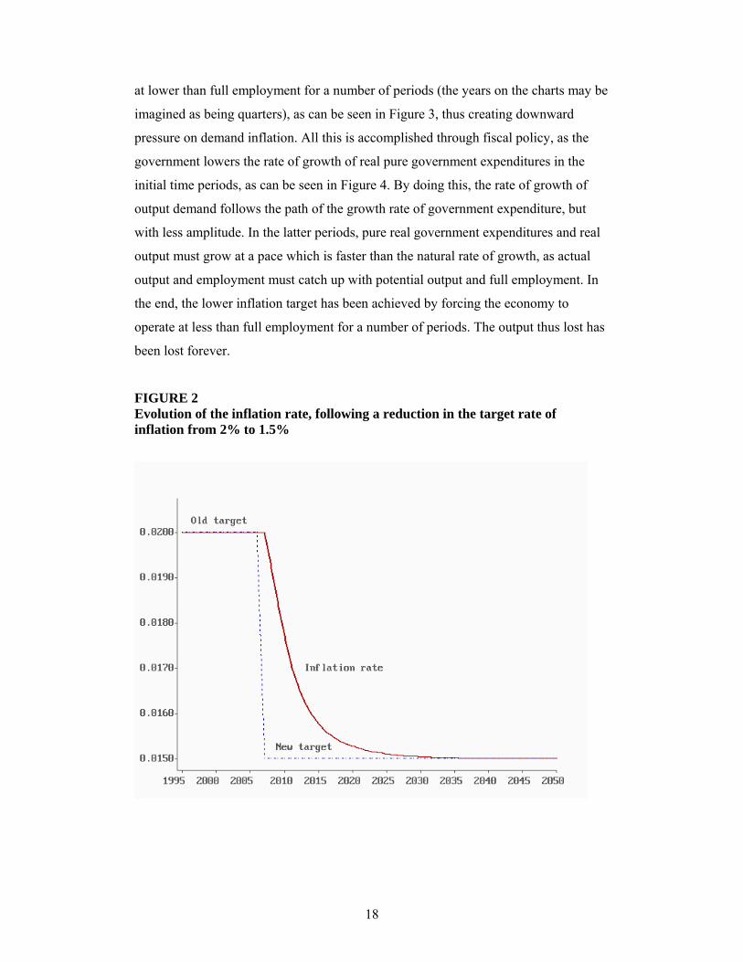
4 show the impact on some of the main variables of the model. First, Figure 2 shows

that fiscal policy is quite able to smoothly get the rate of inflation down to its new

lower target. The lower rate of inflation is achieved by getting the economy to operate

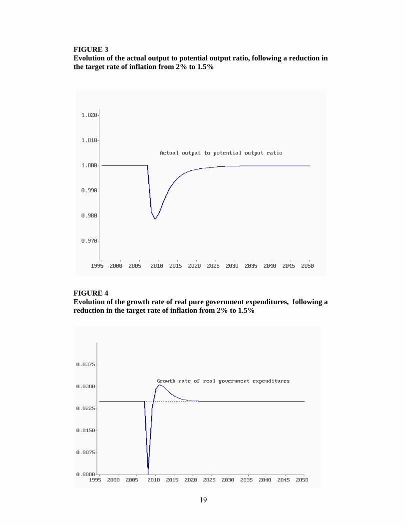
18

at lower than full employment for a number of periods (the years on the charts may be

imagined as being quarters), as can be seen in Figure 3, thus creating downward

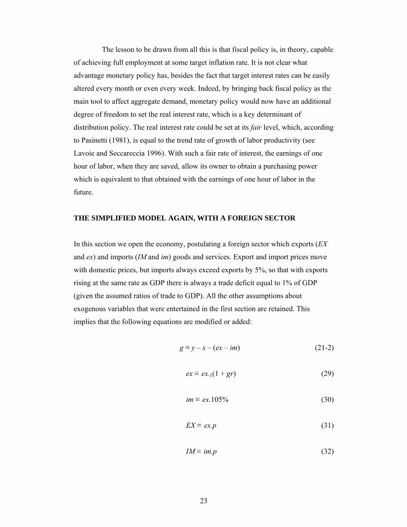
pressure on demand inflation. All this is accomplished through fiscal policy, as the

government lowers the rate of growth of real pure government expenditures in the

initial time periods, as can be seen in Figure 4. By doing this, the rate of growth of

output demand follows the path of the growth rate of government expenditure, but

with less amplitude. In the latter periods, pure real government expenditures and real

output must grow at a pace which is faster than the natural rate of growth, as actual

output and employment must catch up with potential output and full employment. In

the end, the lower inflation target has been achieved by forcing the economy to

operate at less than full employment for a number of periods. The output thus lost has

been lost forever.

FIGURE 2 Evolution of the inflation rate, following a reduction in the target rate of inflation from 2% to 1.5%

19

FIGURE 3 Evolution of the actual output to potential output ratio, following a reduction in the target rate of inflation from 2% to 1.5%

FIGURE 4 Evolution of the growth rate of real pure government expenditures, following a reduction in the target rate of inflation from 2% to 1.5%

20

As a second experiment, let us assume that households decide to raise their

propensity to consume out of disposable income (the α1 coefficient is moved up,

through a higher α10). This should initially lead to an increase in aggregate demand

and hence in inflation. Indeed inflation rises, only to gradually go back to its target

level. Figure 5 shows the evolution of the growth rate of pure government

expenditure, and that of actual output, as fiscal policy attempts to mitigate the

inflationary effects of the increase in private spending.

FIGURE 5 Evolution of the growth rate of real output and of the growth rate of pure real government expenditures, following an increase in the propensity to consume out of disposable income

As a third and final experiment, let us assume that the central bank, acting

on the lobby of rentiers, decides to raise the real rate of interest from 1% to 7%. What

will occur? Figure 6 shows the evolution of the inflation rate. With the initial increase

in interest outlays out of government debt, there is an increase in private expenditure,

which leads to a brief and small increase in the inflation rate, as can be seen in Figure

21

6. However, immediately afterwards, the inflation rate drops briskly, finally coming

back to its initial target level after some overshooting. What happens is that, as can be

seen in Figure 7, as the private sector reacts with a one-period lag to the new higher

real interest rate, they decide to reduce their propensity to spend out of disposable

income, thus plunging the economy into a recession. The fiscal authorities, also with a

lag, try to maintain the economy close to full employment by hiking up the rate of

growth of real pure government expenditures. Eventually, the economy comes back to

full employment at the natural rate of growth. However, as can be seen from Figure 8,

all this adjustment can only occur if the government, and financial markets, accept to

let the public debt to GDP ratio double, from about 41% to nearly 85%. As to the real

deficit to real GDP ratio (not shown here), it peaks for a while at 9%, while its steady

state level rises from 1% to 2%. Once again, despite the fact that the real rate of

interest after tax is much higher than the trend real rate of growth of the economy, all

adjustments are sustainable and the model remains stable.

FIGURE 6 Evolution of the inflation rate, following an increase in the real rate of interest, from 1% to 7%

22

FIGURE 7 Evolution of the growth rate of output and of the growth rate of real pure government expenditures, following an increase in the real rate of interest, from 1% to 7%

FIGURE 8 Evolution of the public debt to GDP ratio, following an increase in the real rate of interest, from 1% to 7%

23

The lesson to be drawn from all this is that fiscal policy is, in theory, capable

of achieving full employment at some target inflation rate. It is not clear what

advantage monetary policy has, besides the fact that target interest rates can be easily

altered every month or even every week. Indeed, by bringing back fiscal policy as the

main tool to affect aggregate demand, monetary policy would now have an additional

degree of freedom to set the real interest rate, which is a key determinant of

distribution policy. The real interest rate could be set at its fair level, which, according

to Pasinetti (1981), is equal to the trend rate of growth of labor productivity (see

Lavoie and Seccareccia 1996). With such a fair rate of interest, the earnings of one

hour of labor, when they are saved, allow its owner to obtain a purchasing power

which is equivalent to that obtained with the earnings of one hour of labor in the

future.

THE SIMPLIFIED MODEL AGAIN, WITH A FOREIGN SECTOR

In this section we open the economy, postulating a foreign sector which exports (EX

and ex) and imports (IM and im) goods and services. Export and import prices move

with domestic prices, but imports always exceed exports by 5%, so that with exports

rising at the same rate as GDP there is always a trade deficit equal to 1% of GDP

(given the assumed ratios of trade to GDP). All the other assumptions about

exogenous variables that were entertained in the first section are retained. This

implies that the following equations are modified or added:

g ≡ y – x – (ex – im) (21-2)

ex ≡ ex-1(1 + gr) (29)

im ≡ ex.105% (30)

EX ≡ ex.p (31)

IM ≡ im.p (32)

24

The balance of payments on current account is equal to the trade balance plus

or minus the flow of interest payments abroad, which are given by r.VF-1, where VF is

the stock of overseas financial wealth, changes in which are equal each period to the

current account balance (CAB). This implies the following equalities:

CAB ≡ EX – IM + r.VF-1 (33)

VF ≡ VF-1 + CAB (34)

The redundant equation, which was NAFA ≡ DEFICIT in the closed economy,

is now equal to:

NAFA ≡ DEFICIT + CAB (D)

This is now a well-known flow-of-funds identity, which forecasters and

analysts now make use of (see Godley 1999).

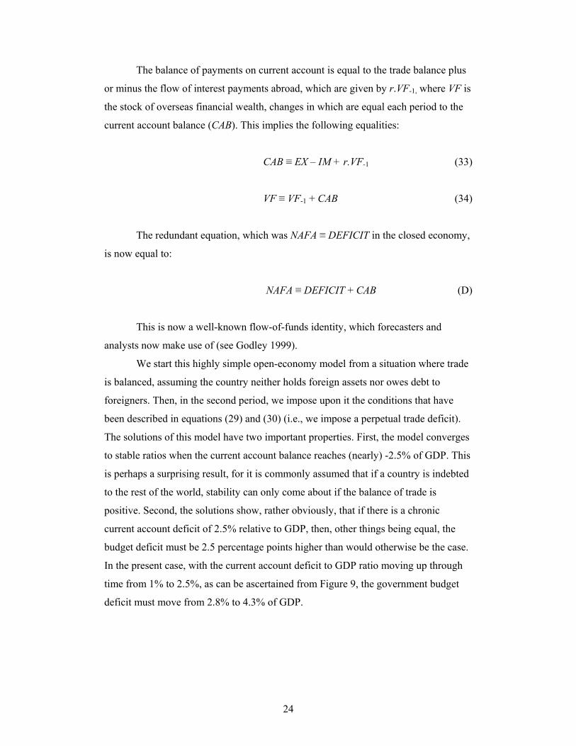
We start this highly simple open-economy model from a situation where trade

is balanced, assuming the country neither holds foreign assets nor owes debt to

foreigners. Then, in the second period, we impose upon it the conditions that have

been described in equations (29) and (30) (i.e., we impose a perpetual trade deficit).

The solutions of this model have two important properties. First, the model converges

to stable ratios when the current account balance reaches (nearly) -2.5% of GDP. This

is perhaps a surprising result, for it is commonly assumed that if a country is indebted

to the rest of the world, stability can only come about if the balance of trade is

positive. Second, the solutions show, rather obviously, that if there is a chronic

current account deficit of 2.5% relative to GDP, then, other things being equal, the

budget deficit must be 2.5 percentage points higher than would otherwise be the case.

In the present case, with the current account deficit to GDP ratio moving up through

time from 1% to 2.5%, as can be ascertained from Figure 9, the government budget

deficit must move from 2.8% to 4.3% of GDP.

25

FIGURE 9 Evolution of the main balances, following the appearance of a trade account deficit that stands forever at 1% of GDP

CONCLUSION

The purposes of this paper are, first, to insist that there exist rules which must govern

the conduct of fiscal policy as the counterpart of stable growth without inflation or

unemployment and to make suggestions as to how those rules should be formulated.

In addition, external trade or current account deficits have implications for deficit

ratios and debt ratios. Finally, we are tentatively drawing two unconventional

conclusions: that an economy (described within a SFC framework) with a real rate of

interest net of taxes which exceeds the real growth rate will not necessarily generate

explosive interest flows, even if the government makes no discretionary attempt to

achieve primary budget surpluses; and, second, that it cannot be assumed that a debtor

country requires a trade surplus if interest payments on debt are not to explode.

We have shown that fiscal policy can deliver sustainable full employment at a

target inflation rate within a stock-flow consistent framework with some arbitrary

interest rate. It follows from our model that if the fiscal stance is not set in the

appropriate fashion (i.e., at a well-defined level and growth rate), then full

employment and low inflation will not be achieved in a sustainable way. As far as we

26

know, New Consensus authors have only shown that monetary policy could provide

full employment at some target inflation rate over a short period, with fiscal policy

left hanging in the air. They have yet to demonstrate such a result over the long run

within a stock-flow consistent framework.

27

REFERENCES

Arestis, P. and Sawyer, M. 2004. “On the Effectiveness of Monetary Policy and of

Fiscal Policy.” Review of Social Economy 62(4): 441–463. Feldstein, M. 1976. “Perceived Wealth in Bonds and Social Security: A Comment.”

Journal of Political Economy 84(2): 331–336. Godley, W. 1999. “Seven Unsustainable Processes: Medium-Term Prospects and

Policies for the United States and the World.” Strategic Analysis, The Levy Economics Institute of Bard College.

Godley, W. and Lavoie, M. 2007. Monetary Economics: An Integrated Approach to

Credit, Money, Income, Production, and Wealth. Basingstoke: Palgrave Macmillan.

Juniper, J. and Mitchell, B. 2005. “Towards a Spatial Keynesian Macroeconomics.”

Working Paper 05-09, Center for Full Employment and Equity, University of Newcastle.

Lavoie, M. 2006. “A Post-Keynesian Amendment to the New Consensus on Monetary

Policy.” Metroeconomica 57(2): 165–192. Lavoie, M. and Seccareccia, M. 1996. “Central Bank Austerity Policy, Zero-Inflation

Targets, and Productivity Growth in Canada.” Journal of Economic Issues 30(2): 533–544.

Pasinetti, L.L. 1981. Structural Change and Economic Growth. Cambridge:

Cambridge University Press. Schlicht, E. 2006. “Public Debt as Private Wealth: Some Equilibrium

Considerations.” Metroeconomica 57(4): 494–520. Setterfield, M. 2005. “Central Bank Behaviour and the Stability of Macroeconomic

Equilibrium: A Critical Examination of the ‘New Consensus’.” In P. Arestis, M. Baddeley, and J. McCombie (eds.) The New Monetary Policy: Implications and Relevance. Cheltenham: Edward Elgar.

Wray, R. 1998. Understanding Modern Money: The Key to Full Employment and

Price Stability. Cheltenham: Edward Elgar.