working paper n - african development bank · alternative production centers in south africa and...
TRANSCRIPT

1
Working Paper No 272
Abstract
Despite efforts to increase integration within Africa,
product markets remain segmented between
countries. This paper examines the magnitude of
price gaps, known as the border-effect, between
Lesotho and South Africa using retail price data for
49 products in 35 cities over the period 2006–2009.
Using a production–consumption pair approach, we
estimate that crossing the border between South
Africa and Lesotho is associated with an absolute
product price gap that widened from 18 percent in
2006 to 29 percent in 2009. The structure of relative
prices also differs markedly, revealing a lack of
convergence to a common set of internal relative
prices. These results are robust to the choice of
alternative production centers in South Africa and
the imposition of distance thresholds between region
pairs. The results indicate that the border between
South Africa and Lesotho remains an impediment to
trade flows and price competition, despite their joint
membership in a customs union and monetary area.
Rights and Permissions
All rights reserved.
The text and data in this publication may be reproduced as long as the source is cited. Reproduction for commercial purposes
is forbidden. The WPS disseminates the findings of work in progress, preliminary research results, and development
experience and lessons, to encourage the exchange of ideas and innovative thinking among researchers, development
practitioners, policy makers, and donors. The findings, interpretations, and conclusions expressed in the Bank’s WPS are
entirely those of the author(s) and do not necessarily represent the view of the African Development Bank Group, its Board
of Directors, or the countries they represent.
Working Papers are available online at https://www.afdb.org/en/documents/publications/working-paper-series/
Produced by Macroeconomics Policy, Forecasting, and Research Department
Coordinator
Adeleke O. Salami
This paper is the product of the Vice-Presidency for Economic Governance and Knowledge Management. It is part
of a larger effort by the African Development Bank to promote knowledge and learning, share ideas, provide open
access to its research, and make a contribution to development policy. The papers featured in the Working Paper
Series (WPS) are those considered to have a bearing on the mission of AfDB, its strategic objectives of Inclusive
and Green Growth, and its High-5 priority areas—to Power Africa, Feed Africa, Industrialize Africa, Integrate
Africa and Improve Living Conditions of Africans. The authors may be contacted at [email protected].
Correct citation: Nchake, M. A., L. Edwards and T. N. Kaya (2017), Price effects of borders between Lesotho and South Africa,
Working Paper Series N° 272, African Development Bank, Abidjan, Côte d’Ivoire.

1
Price effects of borders between Lesotho and South Africa 1
Mamello A. Nchake, Lawrence Edwards and Tresor N. Kaya
JEL Classification: F14, F15
Keywords: Product market integration; Trade costs, Distance; Border effect
1 Mamello A. Nchake (Corresponding author: [email protected]), Department of Economics, National University of Lesotho and School of Economics, University of Cape Town. Lawrence Edwards ([email protected]), School of Economics, University of Cape Town, Rondebosch, Cape Town 7701. Tresor N. Kaya ([email protected]), School of Economics, University of Cape Town, Rondebosch, Cape Town 7701. Authors are grateful for the generous support provided by AERC/AfDB through a research fellowship. This work has benefited greatly from comments and suggestions from the staff in the Development Research Department of African Development Bank, in particular, Dr. Emelly Mutambatsere. The views expressed in this paper are those of the authors. They are grateful for the Exploratory Research Grant (ref. 223) provided for data collection by the Private Enterprise Development in Low-Income Countries (PEDL) research initiative of the Centre for Economic Policy Research (CEPR), and the Department for International Development (DFID).

2
1. Introduction
Understanding the extent to which trade costs affect product market integration is an important
step towards the implementation of well-targeted policies to improve regional integration
(Brenton, Portugal-Perez, and Régolo, 2014). This is of particular importance to Africa where
high transport barriers (such as underdeveloped transport infrastructure and poor, but costly
transport services), poor trade facilitation, and trade barriers have been shown to impede cross-
border intra-Africa trade flows (Longo and Sekkat 2004; Njinkeu, Wilson and Fosso, 2008;
Portugal-Perez and Wilson, 2008). In addition to restricting trade, national borders segment
product markets, causing price gaps beyond what is explained by distance (Rodrik, 2000), “the
border effect,”2 as well as a failure of prices to co-move (Engel and Rogers, 1996; Beck and
Weber, 2001; Parsley and Wei, 2001). Within Africa, these border effects are estimated to be
large, causing prices to deviate by 7 to 30 percent (Versailles, 2012; Aker, Klein, O’Connell,
and Yang, 2014; Brenton Portugal-Perez, and Régolo, 2014; Balchin, Edwards, and Sundaram,
2015).
A limitation of these studies, however, is that the estimated border effects encompass many
factors. First, the estimates of the border effect capture the cumulative effect of many policies
or barriers to integration, not only those attributable to border procedures. For example, price
gaps may reflect differences in import tariff, sales tax or value added tax, product market
regulations, and exchange rates, in addition to costs associated with complying with border
regulations. Second, most studies using price data in developing economies, particularly in
Africa, do not account for the spatial relationship between consumption and production
locations, which is likely to undermine the magnitude of trade costs in product markets
(Anderson, Schaefer, and Smith, 2013; Kano, Kano, and Takechi, 2013). Some studies (for
example, Versailles, 2012, Aker et al., 2014) attempted to solve this problem by restricting the
model to city pairs with distances less than a certain threshold, but the difficulty and somewhat
arbitrary decision that comes with selecting the right threshold does not fully solve the problem.
This study uses a production–consumption approach to identify the effect of border-related
costs on product market integration between Lesotho and South Africa. This approach provides
a more precise measure of the size of border effects that considers spatial relationships between
2 The border effect is the additional unexplained variation in prices between cities in different countries beyond
what can be explained by physical distance. A strong theoretical assumption was that, all being equal, lower trade
costs due to integration between cities or regions on either side of an international border should be associated
with increased price integration in the product market.

3
production and consumption locations. In using this identification strategy, we are able to deal
with selection effects commonly found in the literature that bias distance estimates downwards
and border effects upwards (Anderson, Schaefer, and Smith, 2010; Borraz et al., 2016).
In the paper, we make three contributions. First, the study focuses on Lesotho and South Africa
that have long history of integration policies. Lesotho is an “island–state” within the borders
of South Africa. There is a high degree of mobility of people (no visas are required), and the
countries are fully integrated in terms of the flow of goods through their longstanding
membership in the Southern African Customs Union (SACU). The countries also pursue a
common monetary and exchange rate policy through their membership of the Common
Monetary Area (CMA). Value added tax rates are also aligned. Finally, South African retail
chains have strong presence in the Lesotho market. Over 80 percent of its consumer products
are imported from South Africa (UNCTAD, 2014).3 The country pairs present a “benchmark”
case of integration espoused by many of the Regional Economic Communities within Africa.
This paper assesses the extent to which these policies have been effective in integrating product
markets.
Second, the study uses unique disaggregated product price data, available for 49 products
across 35 cities and towns, over the period 2006–2009. This data set is collected by statistical
agencies in the selected countries for the construction of the national consumer price index
(CPI). The data are collected following similar procedures and are comparable in terms of
product description.
Third, the paper tests the robustness of these results using alternative production centers within
South Africa and the imposition of different distance thresholds between city pairs. Further, in
addition to analyzing absolute price gaps, the paper compares the structure of relative prices
between South Africa and Lesotho. In integrated markets, prices are expected to converge to a
common set of internal relative prices.
The results show that border effects remain large between and within Lesotho and South Africa.
Crossing the border between South Africa and Lesotho is associated with an absolute product
price gap of 21.5 percent. This border effect has increased over the period, rising from 18
3 Data on Lesotho’s imports from South Africa show that, over the past decade, the majority of Lesotho’s consumer products are sources from South Africa. For example, Lesotho’s trade deficit for South Africa’s imports range from US$6.9 billion in 2009 to US$11.4 billion in 2015, with a high proportion of these products covering clothing and footwear, foodstuffs, and vegetable products. The data are obtained from the South Africa’s department of trade and industry, as well as downloaded from the UNCTAD depository of trade statistics (2014). Accessed from: http://knoema.com/UNCTADIMPTOTAL2014/merchandise-trade-matrix-imports-and-exports-of-total-all-products-annual-1995-2013
4
percent in 2006 to 29 percent in 2009. Relative prices also differ markedly between South
Africa and Lesotho, compared to within South Africa. The results are robust to the choice of
alternative production centers in South Africa. In addition, the coefficient on distance is high
in comparison to developed countries in North America and Europe. High trade costs,
therefore, pose a further impediment to the integration of product markets with and between
South Africa and Lesotho. These results reveal that product markets remain segmented between
Lesotho and South Africa, despite their geographical proximity and joint membership in the
customs union and monetary area.
The remainder of this paper is structured as follows: In Section 2, we review the theory and
empirical evidence on estimating product market integration and border effects. In Section 3,
we outline the identification strategy and empirical analysis; In Section 4 the data is described
and we present descriptive statistics on the integration of product markets. In Section 5, we
provide the empirical estimates and test the robustness of the results. We extend the analysis
of border effects to cover relative price integration in Section 6. Finally, in Section 7, we
conclude the paper and discuss policy implications.
2. Theory and evidence
The central theory behind the price-based measure of product market integration is based on
the Law of One Price (henceforth, the LOP). According to the LOP, prices of similar products
expressed in the same currency should, under competitive conditions and no transport costs,
equalize across all locations, nationally and internationally. In practice, the LOP does not hold,
as product prices are affected by trade costs and other impediments to trade. Nevertheless, even
in this case, the price gap across markets should not exceed the transactions costs. This
relationship is denoted by the arbitrage condition:
|P𝑖,𝑘,𝑡 − P𝑗,𝑘,𝑡| ≤ t𝑖𝑗,𝑘 , (1)
where P𝑖𝑘,𝑡 and P𝑗𝑘,𝑡 are the prices (in common currency) of product k, in locations i and j,
respectively, and t𝑖𝑗,𝑘 is the ad valorem equivalent of transaction costs involved in trading
product k between location i and j.4 The inequality condition in Equation (1) states that the
4 Generally, these include all border-related costs (such as delays and burdens of doing business in
another country and under another legal system) and non-border related costs that are incurred in
transporting the good from the origin to its final destination (such as distance and geographical
irregularities).

5
absolute value of price gaps between two markets is bounded by the no-arbitrage condition
(Baulch, 1997). If optimal prices between two markets (i and j) lie within the constraint, then
their price gaps are smaller than trade costs, and no trade takes place.5 If price differences
exceed trade costs, then economic agents arbitrage away the price gaps by trading the product
between the markets.
The common approach to estimating the impact of trade costs on price gaps within and between
countries has been to impose the equality constraint in Equation (1) on all price pairs and
estimate a gravity style model such as:
|𝑝𝑖,𝑘,𝑡 − p𝑗,𝑘,𝑡| = α0 + α1ldist𝑖𝑗 + α2border𝑖𝑗 + γ𝑘 + γ𝑡 + ε𝑖𝑗,𝑡 (2)
where pi,k,t and pj,k,t are the log prices (in common currency) of product k, in location i and j,
respectively; ldist𝑖𝑗 is the log bilateral distance between locations i and j; and border is a
dummy variable equal to 1 if locations i and j are in different countries. The “border-effect”
coefficient α2 measures the marginal price gap between countries relative to the mean price
gap within countries (captured by α0) that is not explained by distance. Gorodnichenko and
Tesar (2009) extended this to account for differences in within country distributions of prices
between the countries by including a country-specific fixed effect.6
The relationship in Equation (2) has formed the basis of much of the available empirical
research on price integration. Some studies applied the gravity model on aggregate CPI data
where the volatility of price differences between markets was used as the dependent variable.
Engel and Rogers (1996), for example, examined the nature of deviations from PPP using 14
disaggregated consumer price indices for the 23 US and Canada cities, for the period 1978–
1994. Their results revealed that crossing the US–Canada border was equivalent to shipping a
good 75,000 km although Gorodnichenko and Tesar (2009) estimated that this falls to 47 km
once cross-country heterogeneity in relative prices is accounted for. Other studies using price
index data include Engel and Rogers (2001) and Beck and Weber (2001) for Europe; Parsley
and Wei (2001) for central Asia, and Rogers and Smith (2001) for the North American Free
Trade Agreement (NAFTA) countries.
5 This is the case where there are two markets, which are highly segmented but have similar demand
and supply characteristics. 6 The study argues that if not accounted for, the presence of cross-country heterogeneity may bias the
estimates of the border effect upwards as they do not distinguish between the border frictions and the
effect of trade between countries with different price distributions, and thus overstate the true effect of
national borders on price differences. The coefficient α2 now measures the marginal price gap between
countries relative to the mean price gap within the omitted country.
6
However, the use of price indices to measure product market integration is problematic, as
indices cannot be used to measure differences in price levels. Further, their use induces
potential aggregation bias and amplifies cross-country deviations in relative prices (Knetter
and Slaughter, 2001; Engel and Rogers, 2004; Engel, Rogers and Wang, 2005; Broda and
Weinstein, 2008). Other studies have applied the gravity model to estimate the border effect
using disaggregated price level data (Parsley and Wei, 2001; Ceglowski, 2003; Crucini,
Telmer, and Zachariadis, 2003, 2005a; Crucini and Shintani, 2008; Crucini, Shintani and
Tsuruga, 2010; Gopinath, et al., 2011). Using this type of data allows for a comparison of
differences in price levels of goods across locations while accounting for heterogeneity across
products.
A further critique of the earlier literature is their inclusion of all price pairs when estimating
Equation 2. This effectively imposes an equality constraint between price gaps and transaction
cost differences for all price pairs. This is inconsistent with Equation (1) where the price gap
for some price pairs is less than the bilateral transaction costs. The inclusion of price pairs
where the transaction cost is not binding, leads to a downward selection bias in the distance
coefficient estimates and an upward bias in the border effect.
Consequently, recent literature has pursued alternative approaches to deal with this selection
bias. The first approach restricts the sample to include only production and consumption market
pairs (see, for example, Anderson et al. [2010, 2013], Inanc and Zachariadis [2012] and Kano,
Kano, and Takechi [2013]). For example, using data from the Economist Intelligence Unit
(EIU), across 15 US cities, Anderson et al. (2010) found a rise in the distance coefficient once
the sample is restricted to consumption–production pairs.
Borraz, et al. (2016) proposed an alternative approach where they categorized price pairs into
distance bins and then estimated the relationship using quantile regressions. They applied this
approach using 202 products in 333 supermarkets within cities in Uruguay. Consistent with
their expectations, the inclusion of all price pairs leads to an overestimate of the distance-
equivalent border effect between cities. When the upper quantiles of the price distribution
within each distance bin are used, the border effect becomes small and insignificant.
The third approach was proposed by Atkin and Donaldson (2015), who extended the
production–consumption pair method by accounting for imperfect competition and varying
mark-ups across locations. Using data for the US, Nigeria, and Ethiopia, they pointed out that
trade costs will not be accurately estimated by using price gaps for production–consumption
centers if traders charge varying mark-ups.

7
These applications have primarily been used to calculate intra-national trade costs, and not
inter-national trade costs. One reason is that price pairs across countries for equivalent products
are difficult to obtain. The research on Africa using price level data is also limited. Exceptions
include Versailles (2012) who analysed the sources of LOP deviations using disaggregated
monthly product prices for 24 goods in 39 cities across four East African (EAC) countries
(Burundi, Kenya, Rwanda, and Uganda). He estimated an average border effect of 13.6 percent
over the period 2004 to 2008. Brenton Portugal-Perez, and Régolo (2014) estimated lower
border effects for Central and Eastern Africa (7 percent) using 3 agricultural products. Using
narrowly defined agricultural products, Aker et al. (2014) calculated border-related price gaps
of 17 percent for millet, 26 percent for cowpeas, (26 percent) between Niger and Nigeria.
Finally, Balchin, Edwards, and Sundaram (2015) estimated an 11.8 percent border-related price
difference for 24 products in 4 Southern African Development Community (SADC) countries
(Botswana, Zambia, Malawi, and South Africa) over the period 2006–2009.
Apart from Aker et al. (2014) who focused on a very narrow set of agricultural products, these
studies on border effects in Africa do not deal with the selection bias associated with the
inclusion of all price-pairs. This paper extends this literature by estimating the deviations from
LOP within and across Lesotho and South Africa, using the production–consumption approach.
Consequently, it is able to control for selection biases that affect the magnitude of the border
effect. To our knowledge, our study is the first to use this approach to estimate the size of the
cross-country border effect using a wide range of product price data in Africa.
3. Data description and sources
This study draws on disaggregated product price data obtained from the Bureau of Lesotho and
Statistics South Africa. The price database is made up of monthly product prices used for the
construction of the consumer price indices (CPI) of Lesotho and South Africa. The prices are
expressed in terms of the South African Rand (ZAR) and are defined by detailed product
descriptions, including units (and in the case of Lesotho, brand names). This allows for a
comparison of prices of similar products across locations and across time. The two data sets
were then matched using unique product descriptions, which were created using individual
product and unit names.7
7 For a detailed list of product descriptions, see Table A.1 in the appendix.

8
Distances between city pairs are calculated using data obtained from Google maps
(https://maps.google.co.za/) and travel math (www.travelmath.com/).8 Distance is calculated
as the shortest distance by road between the centroids of the cities. For example, the shortest
distance by road between Maseru, the capital of Lesotho and Johannesburg is 409 km.9
The final data base used in the empirical analysis is comprised of monthly price observations
for 49 narrowly defined products over 35 towns/cities in South Africa (25) and Lesotho (10),
over the period 2006 to 2009. Table 1 presents the summary information. Table A.1 in the
appendix provides more detailed descriptions of each product.
Table 1: Description of data for Lesotho and South Africa Variable South Africa Lesotho
Period of analysis 2006–2009 2006–2009
Number of cities and towns 25 10
Number of product groups 10 10
Number of products 49 49
Products are categorized into 10 different groups including food products, alcoholic beverages,
clothing and footwear, household furniture, and equipment as presented in Table 2. All
products are traded between South Africa and Lesotho.
Table 2: Number of products by product groups Product groups Number of observations Number of products
All pairs Prod–cons pairs Frequency Percent
Alcoholic beverages 30,005 1,961 3 6.1
Clothing and footwear 72,388 4,465 5 10.2
Food 344,013 18,114 25 51.0
Household furniture and equipment 67,945 3,294 6 12.2
Household operations 26,210 1,375 2 4.1
Non-alcoholic beverages 23,734 1,272 2 4.1
Other goods and services 5,581 65 1 2.0
Personal care 31,004 2,275 2 4.1
Tobacco and narcotics 27,476 1761 2 4.1
Transport equipment 5,740 274 1 2.0
Total 634,096 34,856 49 100
Note: The first column (all pairs) includes annual relative prices for all city pairs. The second column only includes
price pairs between Vereeniging (in South Africa) and all other towns/cities in the database.
8 For the purpose of consistency, in this paper we refer to all locations as cities. 9 We also use driving time as an alternative measure of distance. We do not report these estimations
in the paper, as the results are qualitatively similar. The results will be provided by the authors upon
request.

9
4. Empirical methodology
4.1 Identification strategy
This paper adopts a production–consumption approach based on the framework of Anderson
and van Wincoop (2004), and Anderson, Schaefer, and Smith (2013). A key requirement in
this approach is identifying sources of production for each product. This poses a particular
challenge to this study. First, while South Africa is the main production hub in the region,
production of certain products takes place in multiple locations within the country (e.g., beer
is produced in all the cities). Second, while we have specific brand information for some
products sold in Lesotho, we lack the brand-level information for products in South Africa.
The matching of products across South Africa and Lesotho is based on the product description
that is only defined by product name and unit. It is thus difficult to identify the exact production
center of the South African products.
We therefore adopt an alternative strategy by selecting production centers that are most suitable
to the nature of our data. We identify Vereeniging, a town in the Gauteng province within South
Africa, as the main source for all the products in the sample. Vereeniging is located within the
Sedibeng district, which is one of the main industrial hubs in South Africa and produces the
largest share of production in manufacturing.10 It is located within the Gauteng industrial zone
through the OR Tambo and City Deep terminals. This provides manufacturers in this area with
efficient logistics and distribution services for the movement of goods to importing locations.11
Vereeniging also lies on the main transport route from these areas to Lesotho. Consequently,
Vereeniging is regarded as a suitable proxy for the production hub of the products used in the
analysis. Nevertheless, we test the robustness of our findings to alternative production hubs,
including Bloemfontein, Pretoria, and Vanderbijlpark.
4.2 Empirical specification
Given this background, we estimate the following spatial relationship:
|pc,k,t − pp,k,t| = α0 + α1ldistpc + α2ldist2pc+ α3borderpc + γ𝑘 + γ𝑡 + εpc,t (3)
where |pc,k,t − pp,k,t| is the absolute mean log price difference between the production city (p)
(Vereeniging) and the consumption city (c), located in either South Africa or Lesotho. The term
ldistpc represents the log distance from Vereeniging to the consumption location and is included
10 See Table A.4, for a more detailed breakdown of sectoral contributions for each district. 11 The distance from Vereeniging to the City Deep industrial zone terminal is 61km (around a 44-min
drive) and to the OR Tambo terminal is 80 km (or a 56-min drive).
10
to control for transport costs. The square of log of distance (ldist2pc) is included to account for
potential non-linear relationships between price differences and distance in line with the results
found by Garmendia, Llano-Verduras, and Requena-Silventre, (2012) and Gallego and Llano
(2014).
To capture the border effect, the specification includes a dummy variable borderpc equal to one
for city-pairs between Vereeniging and locations in Lesotho and zero for city-pairs within
South Africa. This variable measures the border-related trade costs conditional on transport
costs. Its coefficient (α3) captures the effect of national borders between Lesotho and South
Africa on price differences. Finally, to control for time-invariant heterogeneity across products,
product dummies (γ𝑘) are included. In addition, month dummies (γ𝑡) are included to control
for cyclical factors that are common to both countries. The standard errors reported are
clustered at city level to account for the possibility that the regression errors are not independent
within the cities.
5. Results
5.1 Descriptive statistics
Product price differences within and between countries
We provide an initial description of the degree of product market integration between
production and consumption city-pairs by estimating absolute mean deviations from LOP using
Equation (3). A country-level comparison of average mean absolute log price differences
across all products in the sample, for the period from 2006 to 2009 is illustrated in Figure 1.
11
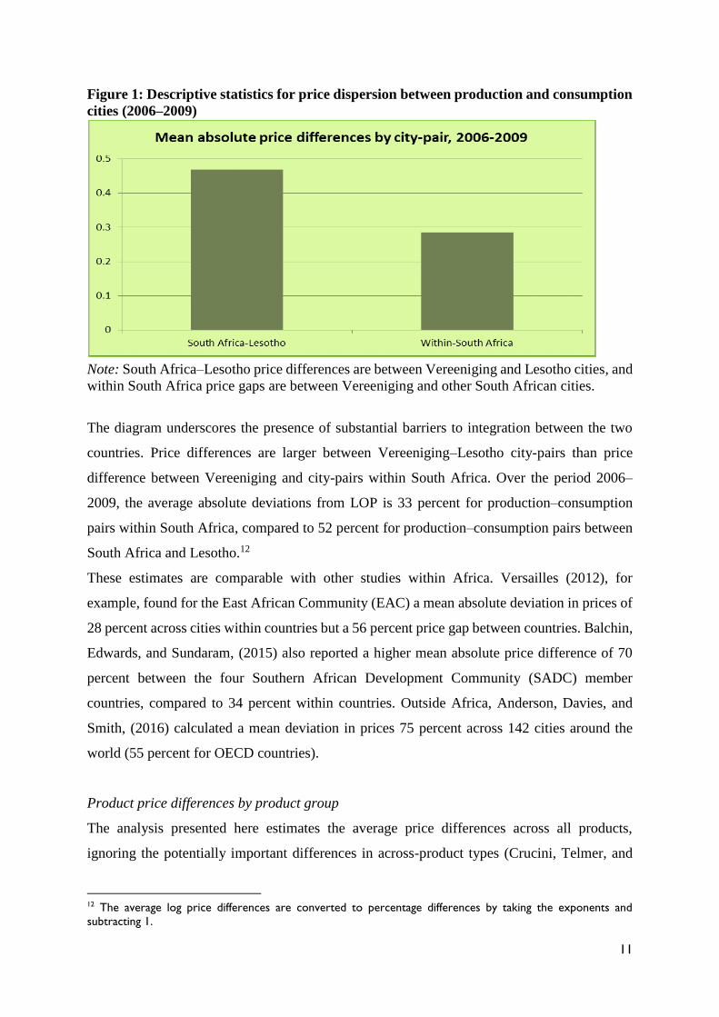
Figure 1: Descriptive statistics for price dispersion between production and consumption
cities (2006–2009)
Note: South Africa–Lesotho price differences are between Vereeniging and Lesotho cities, and
within South Africa price gaps are between Vereeniging and other South African cities.
The diagram underscores the presence of substantial barriers to integration between the two
countries. Price differences are larger between Vereeniging–Lesotho city-pairs than price
difference between Vereeniging and city-pairs within South Africa. Over the period 2006–
2009, the average absolute deviations from LOP is 33 percent for production–consumption
pairs within South Africa, compared to 52 percent for production–consumption pairs between
South Africa and Lesotho.12
These estimates are comparable with other studies within Africa. Versailles (2012), for
example, found for the East African Community (EAC) a mean absolute deviation in prices of
28 percent across cities within countries but a 56 percent price gap between countries. Balchin,
Edwards, and Sundaram, (2015) also reported a higher mean absolute price difference of 70
percent between the four Southern African Development Community (SADC) member
countries, compared to 34 percent within countries. Outside Africa, Anderson, Davies, and
Smith, (2016) calculated a mean deviation in prices 75 percent across 142 cities around the
world (55 percent for OECD countries).
Product price differences by product group
The analysis presented here estimates the average price differences across all products,
ignoring the potentially important differences in across-product types (Crucini, Telmer, and
12 The average log price differences are converted to percentage differences by taking the exponents and
subtracting 1.
12
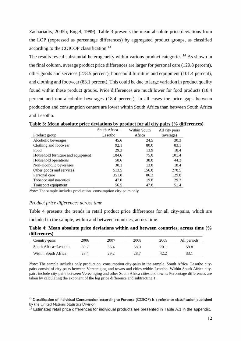
Zachariadis, 2005b; Engel, 1999). Table 3 presents the mean absolute price deviations from
the LOP (expressed as percentage differences) by aggregated product groups, as classified
according to the COICOP classification.13
The results reveal substantial heterogeneity within various product categories.14 As shown in
the final column, average product price differences are larger for personal care (129.8 percent),
other goods and services (278.5 percent), household furniture and equipment (101.4 percent),
and clothing and footwear (83.1 percent). This could be due to large variation in product quality
found within these product groups. Price differences are much lower for food products (18.4
percent and non-alcoholic beverages (18.4 percent). In all cases the price gaps between
production and consumption centers are lower within South Africa than between South Africa
and Lesotho.
Table 3: Mean absolute price deviations by product for all city pairs (% differences)
Product group
South Africa–Lesotho
Within South
Africa
All city pairs
(average)
Alcoholic beverages 45.6 24.5 30.3
Clothing and footwear 92.1 80.0 83.1
Food 29.3 13.9 18.4
Household furniture and equipment 184.6 75.8 101.4
Household operations 58.6 38.8 44.3
Non-alcoholic beverages 30.1 13.8 18.4
Other goods and services 513.5 156.8 278.5
Personal care 351.8 86.3 129.8
Tobacco and narcotics 47.0 19.8 29.3
Transport equipment 56.5 47.8 51.4
Note: The sample includes production–consumption city-pairs only.
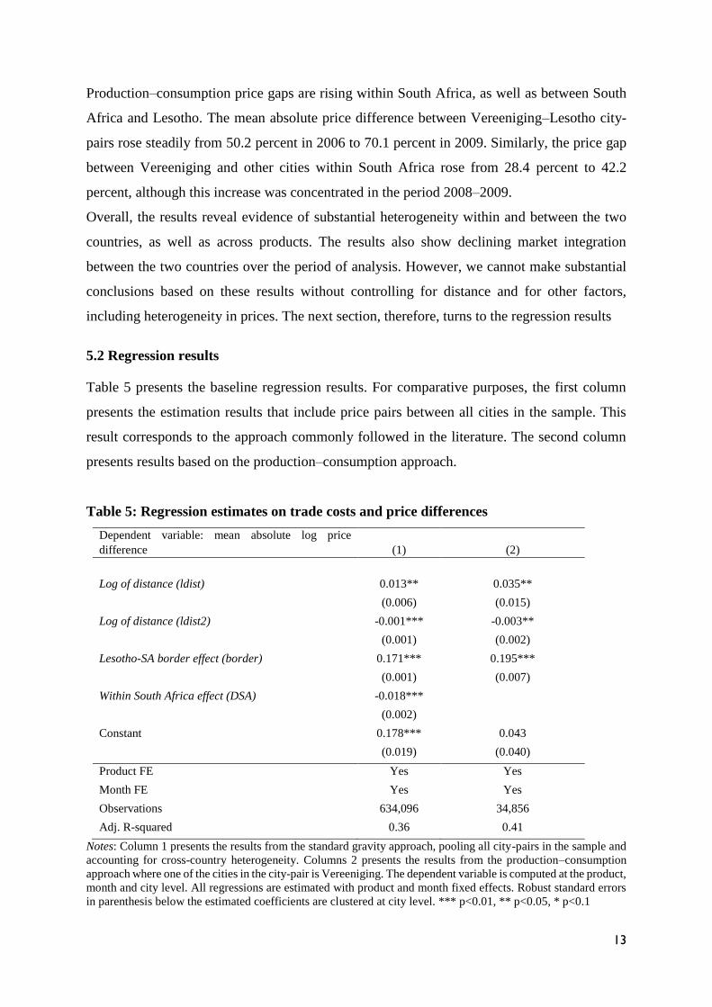
Product price differences across time
Table 4 presents the trends in retail product price differences for all city-pairs, which are
included in the sample, within and between countries, across time.
Table 4: Mean absolute price deviations within and between countries, across time (%
differences)
Country-pairs 2006 2007 2008 2009 All periods
South Africa–Lesotho 50.2 56.4 58.9 70.1 59.8
Within South Africa 28.4 29.2 28.7 42.2 33.1
Note: The sample includes only production–consumption city-pairs in the sample. South Africa–Lesotho city-
pairs consist of city-pairs between Vereeniging and towns and cities within Lesotho. Within South Africa city-
pairs include city-pairs between Vereeniging and other South Africa cities and towns. Percentage differences are
taken by calculating the exponent of the log price difference and subtracting 1.
13 Classification of Individual Consumption according to Purpose (COIOP) is a reference classification published
by the United Nations Statistics Division. 14 Estimated retail price differences for individual products are presented in Table A.1 in the appendix.
13
Production–consumption price gaps are rising within South Africa, as well as between South
Africa and Lesotho. The mean absolute price difference between Vereeniging–Lesotho city-
pairs rose steadily from 50.2 percent in 2006 to 70.1 percent in 2009. Similarly, the price gap
between Vereeniging and other cities within South Africa rose from 28.4 percent to 42.2
percent, although this increase was concentrated in the period 2008–2009.
Overall, the results reveal evidence of substantial heterogeneity within and between the two
countries, as well as across products. The results also show declining market integration
between the two countries over the period of analysis. However, we cannot make substantial
conclusions based on these results without controlling for distance and for other factors,
including heterogeneity in prices. The next section, therefore, turns to the regression results
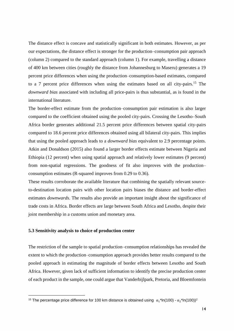
5.2 Regression results
Table 5 presents the baseline regression results. For comparative purposes, the first column
presents the estimation results that include price pairs between all cities in the sample. This
result corresponds to the approach commonly followed in the literature. The second column
presents results based on the production–consumption approach.
Table 5: Regression estimates on trade costs and price differences
Dependent variable: mean absolute log price
difference
(1)
(2)
Log of distance (ldist) 0.013** 0.035**
(0.006) (0.015)
Log of distance (ldist2) -0.001*** -0.003**
(0.001) (0.002)
Lesotho-SA border effect (border) 0.171*** 0.195***
(0.001) (0.007)
Within South Africa effect (DSA) -0.018***
(0.002)
Constant 0.178*** 0.043
(0.019) (0.040)
Product FE Yes Yes
Month FE Yes Yes
Observations 634,096 34,856
Adj. R-squared 0.36 0.41
Notes: Column 1 presents the results from the standard gravity approach, pooling all city-pairs in the sample and
accounting for cross-country heterogeneity. Columns 2 presents the results from the production–consumption
approach where one of the cities in the city-pair is Vereeniging. The dependent variable is computed at the product,
month and city level. All regressions are estimated with product and month fixed effects. Robust standard errors
in parenthesis below the estimated coefficients are clustered at city level. *** p<0.01, ** p<0.05, * p<0.1
14
The distance effect is concave and statistically significant in both estimates. However, as per
our expectations, the distance effect is stronger for the production–consumption pair approach
(column 2) compared to the standard approach (column 1). For example, travelling a distance
of 400 km between cities (roughly the distance from Johannesburg to Maseru) generates a 19
percent price differences when using the production–consumption-based estimates, compared
to a 7 percent price differences when using the estimates based on all city-pairs.15 The
downward bias associated with including all price-pairs is thus substantial, as is found in the
international literature.
The border-effect estimate from the production–consumption pair estimation is also larger
compared to the coefficient obtained using the pooled city-pairs. Crossing the Lesotho–South
Africa border generates additional 21.5 percent price differences between spatial city-pairs
compared to 18.6 percent price differences obtained using all bilateral city-pairs. This implies
that using the pooled approach leads to a downward bias equivalent to 2.9 percentage points.
Atkin and Donaldson (2015) also found a larger border effects estimate between Nigeria and
Ethiopia (12 percent) when using spatial approach and relatively lower estimates (9 percent)
from non-spatial regressions. The goodness of fit also improves with the production–
consumption estimates (R-squared improves from 0.29 to 0.36).
These results corroborate the available literature that combining the spatially relevant source-
to-destination location pairs with other location pairs biases the distance and border-effect
estimates downwards. The results also provide an important insight about the significance of
trade costs in Africa. Border effects are large between South Africa and Lesotho, despite their
joint membership in a customs union and monetary area.
5.3 Sensitivity analysis to choice of production center
The restriction of the sample to spatial production–consumption relationships has revealed the
extent to which the production–consumption approach provides better results compared to the
pooled approach in estimating the magnitude of border effects between Lesotho and South
Africa. However, given lack of sufficient information to identify the precise production center
of each product in the sample, one could argue that Vanderbijlpark, Pretoria, and Bloemfontein
15 The percentage price difference for 100 km distance is obtained using α1*ln(100) - α2*ln(100))2

15
are alternative production centers for products sold in Lesotho. We therefore test the sensitivity
of the results to these alternative production centers.
Table 6: Regression estimates using alternative production centers (1) (2) (3) (4)
Dependent variable: mean absolute
log price difference
Vereeniging Pretoria Vanderbijlpark Bloemfontein
Log of distance (ldist) 0.035** -0.056 0.023* -0.369*** (0.015) (0.050) (0.012) (0.069)
Log of distance (ldist2) -0.003** 0.004 -0.002** 0.031*** (0.002) (0.004) (0.001) (0.006)
Lesotho-SA border effect (border) 0.195*** 0.191*** 0.178*** 0.188***
(0.007) (0.005) (0.008) (0.007)
Constant 0.043 0.336** 0.060 1.224*** (0.040) (0.154) (0.037) (0.209)
Product dummies Yes Yes Yes Yes
Month dummies Yes Yes Yes Yes
Observations 34,856 39,921 30,006 36,547
Adj. R-squared 0.41 0.37 0.29 0.36
Notes: The dependent variable is computed at the product, month, and city level. All regressions are estimated
with product and month fixed effects. The corresponding standard errors in parentheses are clustered at city level.
*** p<0.01, ** p<0.05, * p<0.1
The border coefficient is statistically significant for all regressions. However, the border effect
is larger when Vereeniging is selected as a production center (21.5 percent) than when
Vanderbijlpark, Pretoria, and Bloemfontein are identified as production centers (19.5 percent,
21.0 percent, and 20.7 percent, respectively). The R-squared also indicates that the model
where Vereeniging is a production location better compared to models that use alternative
production centers.16
In contrast, the distance effect is significant and concave only when Vanderbijlpark and
Vereeniging are selected as a production centers. These two towns share similar characteristics
in terms of geographical proximity and commercial distribution. The results obtained for
Pretoria and Bloemfontein are consistent with the fact that Pretoria is more of an administrative
city than a production center, while Bloemfontein has a relatively underdeveloped industrial
sector. Retail prices in these cities are not necessarily good proxies for production prices.
Overall, the results suggest that Vereeniging is a suitable choice as production center.
16 We also estimate Equation (6) using Cape Town and Durban as alternative production centers, but
these results are not reported in the paper. However, the results can be provided upon request from
the authors.

16
5.4 Sensitivity to restriction on distance between city-pairs
We also test our results to different distance thresholds between city-pairs. For example, Aker
et al. (2014) restricted the sample in their market-pair analyses to market pairs that are within
250 km apart. This is because even if spatially relevant source-to-destination location pairs are
used, there is a possibility that some location pairs may still not be relevant, and this may lead
to downward bias in the estimates of the border effect (Borazz et al., 2012).17 To investigate
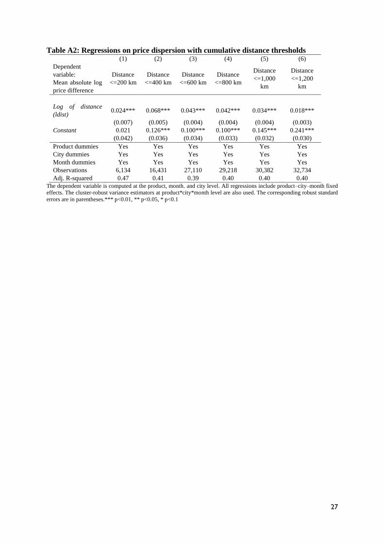
this possibility, we re-estimate Equation (5) with restrictions on distance using distance
cumulative thresholds to determine the price gaps beyond which arbitrage become unlikely.18
The hypothesis is that as distance increases, the border coefficient should also increase.
Figure 1: Regression border effect estimates with cumulative distance thresholds
The results in Figure 2 show that as the distance between city-pairs increases, the border
coefficient declines monotonically up to 600 km and then remains constant at 20 percent.19
This suggests that the results remain quantitatively similar when distance restriction is relaxed,
indicating that the sample bias on the border coefficient cannot be the result of city-pair
composition effect.
17 This approach has been employed by other studies. Borraz et al. (2012), for example, used a quantile regression
approach where they selected the maximum (or 95th percentile) price gap within a range of distance bins while
Aker et al. (2014) restricted the sample in their market-pair analyses to market pairs that are within 250 km
apart. 18 The results are presented in Table A.2 in the appendix 19 See Table A.3 in the appendix section for the basic regression results on border effects and distance,
restricting distance to bilateral city-pairs that are within 200 km, 400 km, 600 km, 800 km and 1000 km
apart.
0.00
0.05
0.10
0.15
0.20
0.25
0.30
Bo
rde
r e
ffe
ct e
stim
ate
Average border effect with distance thresholds

17
5.5 Border-effect overtime
In the preceding analysis, we found that the average border effect across the whole period
(2006–2009) is significant and large. We now turn to an assessment of how the border effect
has changed over time. This is important in assessing how the degree of integration between
the two countries changes over time. To answer this question, we extend Equation (3) to include
interactions of the border dummy with year dummies.20 The coefficients on these interaction
terms reflect the marginal effect relative to the base year 2006. The results are presented in
Table 7.
Table 7: Regression estimates for the border effect overtime Dependent variable: mean absolute
log price difference
(1) (2) (3) (4)
Vereeniging Vanderbijlpark Pretoria Bloemfontein
Log of distance (ldist) 0.034*** 0.026 0.007 -0.233
(0.010) (0.021) (0.045) (0.139)
Log of distance (ldist2) -0.003*** -0.002 -0.001 0.019
(0.001) (0.002) (0.004) (0.012)
Lesotho–SA border effect 0.161*** 0.144*** 0.147*** 0.177***
(0.013) (0.014) (0.007) (0.012)
Lesotho–SA border effect,2007 0.030*** 0.020* 0.029*** -0.010
(0.010) (0.013) (0.008) (0.010)
Lesotho–SA border effect,2008 0.046*** 0.048*** 0.081*** 0.036***
(0.010) (0.010) (0.012) (0.011)
Lesotho–SA border effect,2009 0.050*** 0.039*** 0.020* -0.001
(0.011) (0.014) (0.010) (0.011)
Constant 0.038* 0.091 0.168 0.894**
(0.036) (0.060) (0.139) (0.408)
Product FE Yes Yes Yes Yes
Month FE Yes Yes Yes Yes
Observations 34,856 30,006 39,921 36,547
Adj. R-squared 0.41 0.35 0.36 0.36
Notes: The dependent variable is computed at the product, month, and city level. All regressions are estimated
with product and month fixed effects. The coefficients on the interaction variables with year dummies represent
the marginal effects relative to the border effect in 2006. The corresponding standard errors in parentheses are
clustered at city level. *** p<0.01, ** p<0.05, * p<0.1
From column 1, the results reveal no evidence of further integration in product markets between
Lesotho and South Africa over the period of analysis. The average border related price
differences increased from 18.1 percent in 2006 to 29.6 percent in 2009. This suggests that
price gaps due to transaction costs incurred at the border between Lesotho and South Africa
were increasing over the period 2006–2009, despite the trade and monetary integration between
20 |Pp,k,t − Pc,k,t| = α0 + α1ldistpc + α2ldist2pc+ α3border𝑝𝑐 ∗ D2006+ α4border𝑝𝑐 ∗ D2007+ α5border𝑝𝑐 ∗
D2008+ α6border𝑝𝑐 ∗ D2009 + γ𝑘 + εpc,t
18
these two countries.
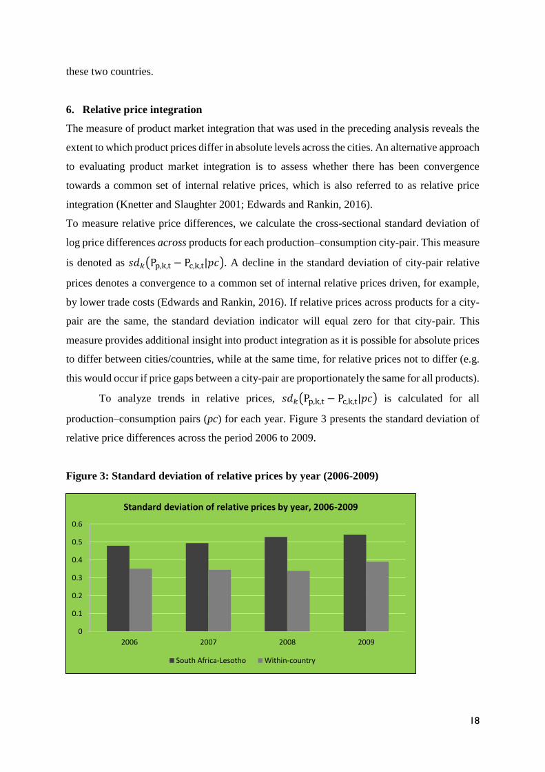
6. Relative price integration
The measure of product market integration that was used in the preceding analysis reveals the
extent to which product prices differ in absolute levels across the cities. An alternative approach
to evaluating product market integration is to assess whether there has been convergence
towards a common set of internal relative prices, which is also referred to as relative price
integration (Knetter and Slaughter 2001; Edwards and Rankin, 2016).
To measure relative price differences, we calculate the cross-sectional standard deviation of
log price differences across products for each production–consumption city-pair. This measure
is denoted as 𝑠𝑑𝑘(Pp,k,t − Pc,k,t|𝑝𝑐). A decline in the standard deviation of city-pair relative
prices denotes a convergence to a common set of internal relative prices driven, for example,
by lower trade costs (Edwards and Rankin, 2016). If relative prices across products for a city-
pair are the same, the standard deviation indicator will equal zero for that city-pair. This
measure provides additional insight into product integration as it is possible for absolute prices
to differ between cities/countries, while at the same time, for relative prices not to differ (e.g.
this would occur if price gaps between a city-pair are proportionately the same for all products).
To analyze trends in relative prices, 𝑠𝑑𝑘(Pp,k,t − Pc,k,t|𝑝𝑐) is calculated for all
production–consumption pairs (pc) for each year. Figure 3 presents the standard deviation of
relative price differences across the period 2006 to 2009.
Figure 3: Standard deviation of relative prices by year (2006-2009)
0
0.1
0.2
0.3
0.4
0.5
0.6
2006 2007 2008 2009
Standard deviation of relative prices by year, 2006-2009
South Africa-Lesotho Within-country

19
Figure 3 reveals substantial differences in relative prices across goods within South Africa and
between Lesotho and South Africa.21 The standard deviation is lower between production and
consumption pairs in South Africa (0.36) than between South Africa and Lesotho (0.52).
Relative prices also seem to be diverging, particularly between South Africa and Lesotho. The
border, therefore, appears to impose costs that affect the average absolute price gap, as well as
relative price gaps, and these affects are increasing over time.
To further tease out this relationship, we re-estimate Equation (5) but with the standard
deviation of log price differences as the dependent variable.22 The results are presented in Table
8.
Table 8: Regression on border effect estimates using relative prices (1) (2) (3) (4)
Dependent variable: standard deviation
of log relative prices
Vereeniging Pretoria Vanderbijlpark Bloemfontein
Log of distance (ldist) 0.043*** 0.041 0.047** -0.094
(0.010) (0.055) (0.023) (0.107)
Log of distance (ldist2) -0.005*** -0.003 -0.005* 0.009 (0.001) (0.005) (0.003) (0.009)
Lesotho–SA border effect (border) 0.029*** 0.037*** 0.014* 0.045*** (0.008) (0.004) (0.007) (0.009)
Constant 0.245*** -0.011 0.257*** 0.500 (0.025) (0.166) (0.051) (0.323)
Product FE Yes Yes Yes Yes
Observations 2,459 2,592 2,461 2,554
Adj. R-squared 0.72 0.77 0.66 0.71
Notes: The dependent variable is computed at the city-pair level. All regressions are estimated with product fixed
effects. The corresponding standard errors in parentheses are clustered at city level. *** p<0.01, ** p<0.05, *
p<0.1
The results reveal a significant distortionary effect of the border on relative prices between
South Africa and Lesotho, even after accounting for distance. This result remains robust to the
use of alternative production centers. In conclusion, the border not only distorts absolute prices,
it also distorts relative prices.
7. Conclusion
This paper examines the extent to which product markets are integrated between Lesotho and
South Africa. Key to this study is the estimation of the magnitude of border effects, using the
spatial production–consumption approach. The results reveal that product markets are not fully
integrated between Lesotho and South Africa. Price differences between countries are larger
21 The data only includes the production–consumption pairs. 22 𝑠𝑑𝑘(pp,k,t − pc,k,t\𝑝𝑐) = α0 + α1ldistpc + α2ldist2pc+ α3border𝑝𝑐 + γ𝑘 + εpc,t

20
than within countries. Crossing the national border increases price differences between South
Africa and Lesotho by 21.5 percent over the full 2006 to 2009 period. This average masks a
border effect that is rising over time from 17 percent in 2006 to 26 percent in 2009. The
structure of relative prices also differs markedly, revealing a lack of convergence to a common
set of internal relative prices. These results are robust to the choice of alternative production
centers in South Africa and the imposition of distance thresholds between region pairs.
The results indicate that the border between South Africa and Lesotho remains an impediment
to trade flows and price competition, despite their joint membership in a customs union and
monetary area. Trade agreements and monetary unions alone may not be sufficient to eliminate
border-related impediments to international trade and competition. Additional mechanisms to
enhance the efficiency at ports of entry, such as one-stop border posts, need to be considered.

21
References
Aker J. C., M. W. Klein, S. A. O’Connell, and M. Yang (2014). “Borders, Ethnicity and Trade.”
Journal of Development Economics 107: 1–16.
Anderson, J. E., and E. van Wincoop (2004). “Trade Costs.” Journal of Economic Literature
42 (3): 691–751.
Anderson, M., M. Davies, and S. L. S. Smith (2016). “Ethnic Networks and Price Dispersion.”
Review of International Economics 24 (3): 514–535.
Anderson, M. A., K. C. Schaefer, and S. L. S. Smith (2010). “Price Dispersion in Spatial
Perspective: Theory and Evidence.” Available at SSRN: https://ssrn.com/abstract=1275776 or
http://dx.doi.org/10.2139/ssrn.1275776.
Anderson M. A., K. C. Schaefer, and S. L. S. Smith (2013). “Can Price Dispersion Reveal
Distance-related Trade Costs? Evidence from the United States.” Global Economy Journal 13
(2): 151–173.
Atkin, D., and D. Donaldson. (2015) “Who’s Getting Globalized? The Size and Implications
of Intra-National Trade Costs.” NBER Working Paper, No. w21439, National Bureau of
Economic Research, Cambridge, MA.
Balchin, N., L. Edwards, and A. Sundaram (2015). “A Disaggregated Analysis of Product Price
Integration in the Southern African Development Community.” Journal of African Economies
24 (3): 390–415.
Baulch, B. (1997). “Transfer Costs, Spatial Arbitrage, and Testing for Food Market
Integration.” American Journal of Agricultural Economics 79 (2): 477-487.
Beck, G., and A. Weber (2001). “How Wide are European Borders? New Evidence on the
Integration Effects of Monetary Unions.” Working Paper No. 2001/07, Center for Financial
Studies, University of Frankfurt/Main.
Broda C., and D. E. Weinstein (2008). “Understanding International Price Differences Using
Barcode Data.” NBER Research Working Paper Series, No. 14017, National Bureau of
Economic Research, Cambridge, MA.
Borraz, F., A. F. Cavallo, R. Rigobon, and L. Zipitría (2012). “Distance and Political
Boundaries: Estimating Border Effects Under Inequality Constraints.” NBER Research
Working Paper, No. 18122, National Bureau of Economic Research, Cambridge, MA.
Borraz, F., A. Cavallo, R. Rigobon, and L. Zipitria. (2016). “Distance and Political Boundaries:
Estimating Border Effects under Inequality Constraints.” International Journal of Finance and
Economics 21 (1): 3–35.
22
Brenton, P., A. Portugal-Perez, and J. Régolo (2014). “Food Prices, Road Infrastructure, and
Market Integration in Central and Eastern Africa.” Policy Research Working Paper, No. 7003,
World Bank, Washington, DC.
Ceglowski, J. (2003). “The Law of One Price: Intranational Evidence for Canada.” Canadian
Journal of Economics/Revue Canadienne D'Économique 36 (2): 373–400.
Crucini, M. J., and M. Shintani (2008). “Persistence in Law of One Price Deviations: Evidence
from Micro-data.” Journal of Monetary Economics 55 (3): 629–644.
Crucini, M. J., M. Shintani, and T. Tsuruga (2010). “The Law of One Price without the Border:
The Role of Distance versus Sticky Prices.” The Economic Journal 120 (544): 462–480.
Crucini, M. J., C. Telmer, and M. Zachariadis (2003). “Price Dispersion: The Role of Distance,
Borders and Location.” Working Paper No. 12-2003, Tepper School of Business, Carnegie
Mellon University, Pittsburgh, PA.
Crucini M. J., C. I. Telmer, and M. Zachariadis (2005a). “Price Dispersion: The Role of
Borders, Distance and Location.” Society for Economic Dynamics, 2005 Meeting Paper, No.
767, Budapest, June 23–25.
Crucini M. J., C. I. Telmer, and M. Zachariadis (2005b). “Understanding European Real
Exchange Rates.” American Economic Review 95 (3): 724–738.
Edwards, L., and N. Rankin (2016). “Is Africa Integrating? Evidence from Product Markets.”
Journal of International Trade & Economic Development 25 (1): 266–289.
Engel, C. (1999). “Accounting for U.S Real Exchange Rate Changes.” Journal of Political
Economy 107 (3): 507–538.
Engel, C., and J. H. Rogers (1996). “How Wide is the Border?” American Economic Review
86 (5): 1112–1125.
Engel, C. and J.H. Rogers (2001). “Deviations From Purchasing Power Parity: Causes and
Welfare Costs.” Journal of International Economics 55(1): 29-57
Engel, C. and J.H. Rogers (2004). “European Product Market Integration After the Euro.”
Economic Policy 19(39): 347-384.
Engel, C., J. H. Rogers, and S. Wang (2005). “Revisiting the Border: An Assessment of the
Law of One Price Using Very Disaggregated Consumer Price Data.” In R. Driver, P. Sinclair,
and C. Thoenissen, eds., Exchange Rates, Capital Flows and Policy, 187–203. London:
Routledge.
Gallego, N., and C. Llano (2014). “The Border Effect and the Nonlinear Relationship between
Trade and Distance.” Review of International Economics 22 (5): 1016–1048.
23
Garmendia, A., C. Llano-Verduras, and F. Requena-Silventre (2012). “Network and the
Disappearance of the Intra-national Home Bias.” Economic Letters 116 (2): 178–182.
Gopinath, G., P. Gourinchas, C. Hsieh, N. Li (2011). “International Prices, Costs, and Markup
Differences.” American Economic Review 101 (6): 2450–2486.
Gorodnichenko, Y., and L. L. Tesar (2009). “Border Effect or Country Effect? Seattle May Not
Be So Far from Vancouver After All.” American Economic Review 1 (1): 219–241.
Inanc, O., and M. Zachariadis (2012). “The Importance of Trade Costs in Deviations from the
Law-of-One-Price: Estimates Based on the Direction of Trade.” Economic Inquiry 50 (3): 667–
689.
IHS Global Insight (2010). “Assessment of the Effectiveness of Scrapping Schemes for
Vehicles Economic, Environmental, and Safety Impacts.” Report prepared for European
Commission, DG Enterprise and Industry, Final Report, March 2010.
Kano, K., T. Kano, and K. Takechi (2013). “Exaggerated Death of Distance: Revisiting
Distance Effects on Regional Price Dispersions. Journal of International Economics 90: 403–
413.
Knetter, M., and M. Slaughter (2001). “Measuring Product Market Integration.” In M.
Blomstrom and L. Goldberg, eds., Topics in Empirical International Economics, 15–46.
National Bureau of Economic Research Conference Report. Chicago: University of Chicago
Press.
Longo, R., and K. Sekkat (2004). “Economic Obstacles to Expanding Intra-African Trade.”
World Development 32 (8): 1309–1321.
Njinkeu, D., J. S. Wilson, and B. P. Fosso (2008). “Expanding Trade within Africa: The Impact
of Trade Facilitation.” Research Working Paper No. 4790, World Bank, Washington, DC.
Parsley, D. C., and S. J. Wei (2001). “Explaining the Border Effect: The Role of Exchange
Rate Variability, Shipping Costs, and Geography.” Journal of International Economics 55 (1):
87–105.
Portugal-Perez, A., and J. S. Wilson (2008). “Trade Costs in Africa: Barriers and Opportunities
for Reform.” Policy Research Working Paper, World Bank, Washington, DC.
Rodrik, D. (2000). “How Far Will International Economic Integration Go?” Journal of
Economic Perspectives 14 (1): 177–186.
Rogers, J.H., andH.P. Smith.(2001). “Border Effects Within the NAFTA Countries.” Internati
onal Finance Discussion Papers Number 698. Board of Governors of the Federal Reserve Sys
tem.

24
UNCTAD, (2014). Depository of Trade Statistics. Accessed from:
http://knoema.com/UNCTADIMPTOTAL2014/merchandise-trade-matrix-imports-and-
exports-of-total-all-products-annual-1995-2013
Versailles, B. (2012). “Market Integration and Border Effects in Eastern Africa”. CSAE
Working Paper WPS/2012-01, Centre for the Study of African Economies, Oxford.
25
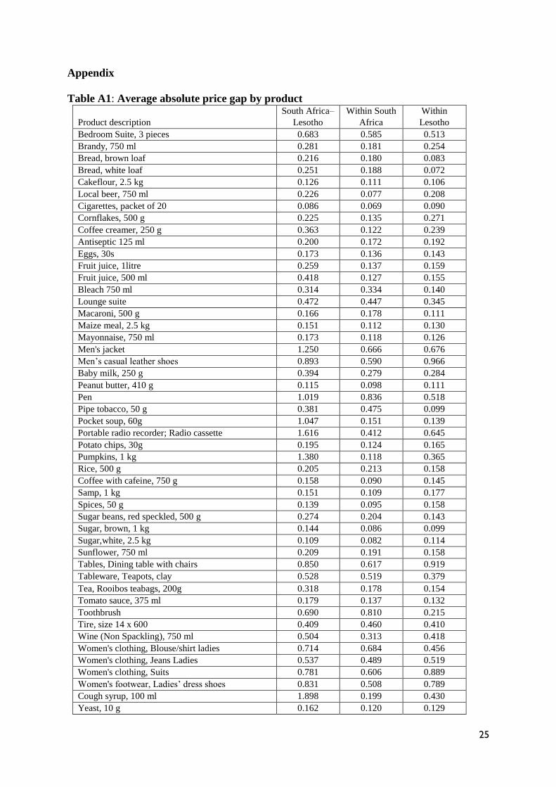
Appendix
Table A1: Average absolute price gap by product
Product description
South Africa–
Lesotho
Within South
Africa
Within
Lesotho
Bedroom Suite, 3 pieces 0.683 0.585 0.513
Brandy, 750 ml 0.281 0.181 0.254
Bread, brown loaf 0.216 0.180 0.083
Bread, white loaf 0.251 0.188 0.072
Cakeflour, 2.5 kg 0.126 0.111 0.106
Local beer, 750 ml 0.226 0.077 0.208
Cigarettes, packet of 20 0.086 0.069 0.090
Cornflakes, 500 g 0.225 0.135 0.271
Coffee creamer, 250 g 0.363 0.122 0.239
Antiseptic 125 ml 0.200 0.172 0.192
Eggs, 30s 0.173 0.136 0.143
Fruit juice, 1litre 0.259 0.137 0.159
Fruit juice, 500 ml 0.418 0.127 0.155
Bleach 750 ml 0.314 0.334 0.140
Lounge suite 0.472 0.447 0.345
Macaroni, 500 g 0.166 0.178 0.111
Maize meal, 2.5 kg 0.151 0.112 0.130
Mayonnaise, 750 ml 0.173 0.118 0.126
Men's jacket 1.250 0.666 0.676
Men’s casual leather shoes 0.893 0.590 0.966
Baby milk, 250 g 0.394 0.279 0.284
Peanut butter, 410 g 0.115 0.098 0.111
Pen 1.019 0.836 0.518
Pipe tobacco, 50 g 0.381 0.475 0.099
Pocket soup, 60g 1.047 0.151 0.139
Portable radio recorder; Radio cassette 1.616 0.412 0.645
Potato chips, 30g 0.195 0.124 0.165
Pumpkins, 1 kg 1.380 0.118 0.365
Rice, 500 g 0.205 0.213 0.158
Coffee with cafeine, 750 g 0.158 0.090 0.145
Samp, 1 kg 0.151 0.109 0.177
Spices, 50 g 0.139 0.095 0.158
Sugar beans, red speckled, 500 g 0.274 0.204 0.143
Sugar, brown, 1 kg 0.144 0.086 0.099
Sugar,white, 2.5 kg 0.109 0.082 0.114
Sunflower, 750 ml 0.209 0.191 0.158
Tables, Dining table with chairs 0.850 0.617 0.919
Tableware, Teapots, clay 0.528 0.519 0.379
Tea, Rooibos teabags, 200g 0.318 0.178 0.154
Tomato sauce, 375 ml 0.179 0.137 0.132
Toothbrush 0.690 0.810 0.215
Tire, size 14 x 600 0.409 0.460 0.410
Wine (Non Spackling), 750 ml 0.504 0.313 0.418
Women's clothing, Blouse/shirt ladies 0.714 0.684 0.456
Women's clothing, Jeans Ladies 0.537 0.489 0.519
Women's clothing, Suits 0.781 0.606 0.889
Women's footwear, Ladies’ dress shoes 0.831 0.508 0.789
Cough syrup, 100 ml 1.898 0.199 0.430
Yeast, 10 g 0.162 0.120 0.129

26
Average 0.421 0.275 0.251
27
Table A2: Regressions on price dispersion with cumulative distance thresholds (1) (2) (3) (4) (5) (6)
Dependent
variable: Distance
<=200 km
Distance
<=400 km
Distance
<=600 km
Distance
<=800 km
Distance
<=1,000
km
Distance
<=1,200
km Mean absolute log
price difference
Log of distance
(ldist) 0.024*** 0.068*** 0.043*** 0.042*** 0.034*** 0.018***
(0.007) (0.005) (0.004) (0.004) (0.004) (0.003)
Constant 0.021 0.126*** 0.100*** 0.100*** 0.145*** 0.241***
(0.042) (0.036) (0.034) (0.033) (0.032) (0.030)
Product dummies Yes Yes Yes Yes Yes Yes
City dummies Yes Yes Yes Yes Yes Yes
Month dummies Yes Yes Yes Yes Yes Yes
Observations 6,134 16,431 27,110 29,218 30,382 32,734
Adj. R-squared 0.47 0.41 0.39 0.40 0.40 0.40
The dependent variable is computed at the product, month. and city level. All regressions include product–city–month fixed
effects. The cluster-robust variance estimators at product*city*month level are also used. The corresponding robust standard
errors are in parentheses.*** p<0.01, ** p<0.05, * p<0.1
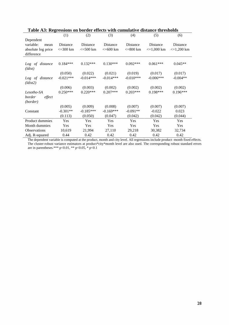
28
Table A3: Regressions on border effects with cumulative distance thresholds (1) (2) (3) (4) (5) (6)
Dependent
variable: mean
absolute log price
difference
Distance
<=300 km
Distance
<=500 km
Distance
<=600 km
Distance
<=800 km
Distance
<=1,000 km
Distance
<=1,200 km
Log of distance
(ldist)
0.184*** 0.132*** 0.130*** 0.092*** 0.061*** 0.045**
(0.050) (0.022) (0.021) (0.019) (0.017) (0.017)
Log of distance
(ldist2)
-0.021*** -0.014*** -0.014*** -0.010*** -0.006*** -0.004**
(0.006) (0.003) (0.002) (0.002) (0.002) (0.002)
Lesotho-SA
border effect
(border)
0.250*** 0.220*** 0.207*** 0.203*** 0.198*** 0.196***
(0.005) (0.009) (0.008) (0.007) (0.007) (0.007)
Constant -0.301** -0.185*** -0.169*** -0.091** -0.022 0.023 (0.113) (0.050) (0.047) (0.042) (0.042) (0.044)
Product dummies Yes Yes Yes Yes Yes Yes
Month dummies Yes Yes Yes Yes Yes Yes
Observations 10,619 21,994 27,110 29,218 30,382 32,734
Adj. R-squared 0.44 0.42 0.42 0.42 0.42 0.42
The dependent variable is computed at the product, month and city level. All regressions include product–month fixed effects.
The cluster-robust variance estimators at product*city*month level are also used. The corresponding robust standard errors
are in parentheses.*** p<0.01, ** p<0.05, * p<0.1

29
Appendix Table A.4: Municipal Sectoral Composition, Gauteng, 2009
Note: CoJ stands for City of Johannesburg and CoT stands for City of Cape Town.
Source: IHS Global Insight (2010)

30