1

WORKING PAPER JANUARY 2020 1

Forecasting grouped time series demand in supply chains 2

Dejan Mircetica,a

, Bahman Rostami-Tabarb, Svetlana Nikolicic

a, Marinko Maslaric

a 3

aUniversity of Novi Sad, Republic of Serbia; 4

bCardiff Business School, Cardiff University, Cardiff, United Kingdom 5

ABSTRACT 6

Demand forecasting is a fundamental component of efficient supply chain management. An accurate 7

demand forecast is required at several different levels of a supply chain network to support the 8

planning and decision-making process in various departments. In this paper, we investigate the 9

performance of bottom-up, top-down and optimal combination forecasting approaches in a supply 10

chain. We first evaluate their forecast performance by means of a simulation study and an empirical 11

investigation in a multi-echelon distribution network from a major European brewery company. For 12

the latter, the grouped time series forecasting structure is designed to support managers’ decisions 13

in manufacturing, marketing, finance and logistics. Then, we examine the forecast accuracy of 14

combining these approaches. Results reveal that forecast combinations produce forecasts than are 15

as accurate as individual approaches. Moreover, we develop a model to analyse the impact of time 16

series characteristics on the effectiveness of each approach. Results provide insights into the 17

interaction among time series characteristics and the performance of these approaches at the 18

bottom level of the hierarchy. Valuable insights are offered to practitioners and the paper closes with 19

final remarks and agenda for further research in this area. 20

Keywords: Supply chain forecasting, Forecast combination, Hierarchical forecasting, Grouped time 21

series forecasting, Time series characteristics. 22

1. INTRODUCTION 23

Demand forecasting is the starting point for most planning and control organizational activities 24

(Rostami-Tabar, Babai, Ducq, & Syntetos, 2015). It is vital to supply chains (SCs), as it provides the 25

basic inputs for the planning and control of all functional areas, including logistics, marketing, 26

production, and finance (Ballou, 2004). Demand forecasting performance is subject to the 27

uncertainty underlying the time series demand a SC is dealing with (Rostami-Tabar, 2013). Therefore, 28

capturing, managing and characterizing uncertainty in SCs represents one of the main problems 29

confronting managers while planning and synchronizing operations in SCs. The demand uncertainty is 30

a Correspondence: D. Mircetic, University of Novi Sad, Trg Dositeja Obradovica 6, 21000 Novi Sad, Republic of

Serbia, Tel: +381 21 485 2433, Email: Dejan.Mircetic@uns.ac.rs.

2

among the most important challenges facing modern SCs (Babai, Ali, & Nikolopoulos, 2012; A. Chen 1

& Blue, 2010; Mircetic, Nikolicic, Stojanovic, & Maslaric, 2017; Syntetos, Babai, Boylan, Kolassa, & 2

Nikolopoulos, 2016; Teunter, Babai, Bokhorst, & Syntetos, 2018; Trapero, Cardos, & Kourentzes, 3

2019), and it poses considerable difficulties in terms of the SC planning and control (Syntetos et al., 4

2016). Hence, the purpose of demand forecasting in SCs is to inform SC planning decisions by 5

providing an accurate estimation of the future demand in a given situation. 6

Demand forecasting for SC often concerns many items. SC forecasters may extrapolate the time 7

series for each Stock Keeping Unit (SKU) individually. However, most of the SC time series have 8

natural groupings of SKUs; that is, the SKUs may be aggregated to get higher levels of forecasts 9

across different dimensions such as geographical areas, customer types, supplier types and product 10

families (Chen & Boylan, 2007). Therefore, various levels of forecasts are required for different parts 11

of SC. The level at which forecasting is performed then it will depend on the function the forecasts 12

are fed into (Rostami-Tabar et al., 2015). For instance, a retailer may use the point-of-sale data to 13

produce forecasts at the store level. However, a manufacturer may use the forecasts of aggregated 14

demand series for the production planning (Chopra & Meindl, 2007). For the transportation manager 15

in charge of the distribution planning, crucial information may include spatial fragmentation of 16

demand, shipments size (replenishment orders) for each distribution channel, the timing of the 17

shipments and the type of product in shipments. Inventory manager might be interested in forecasts 18

related to the type of materials needed at the SKU level, how much will be needed, and when it will 19

arise (Caplice & Sheffi, 2006). Accordingly, SC managers may disaggregate the total demand on the 20

dimensions which are important for a particular party in the chain. This is the moment where the 21

forecasting a single SKU is directed toward the hierarchical forecasting (HF) or grouped forecasting 22

(GF)b. 23

A considerable part of the forecasting literature has been dedicated to methods for single time 24

series, but in reality, there are often many related time series that can be organized hierarchically or 25

in groups (Rostami-Tabar et al., 2015). Hierarchical time series can be represented as a hierarchically 26

organized multiple time series that may be aggregated at several different levels in groups according 27

to the different features (Hyndman, Ahmed, Athanasopoulos, & Shang, 2011). Grouped time series 28

are hierarchical time series that do not impose a unique hierarchical structure in the sense that the 29

order by which the series can be grouped is not unique (Hyndman & Athanasopoulos, 2018). 30

HF naturally reflects important SC characteristics and offers an ample scope for the introduction of 31

innovative forecasting methodologies (Syntetos et al., 2016), improvement of the forecast accuracy 32 b GF can be considered as a special case of HF. Depending on the demand structure of the SC, HF or GF

methodology might be used.

3

and planning, reduction of the overall forecast burden and delivery of the high service level (Caplice 1

& Sheffi, 2006; Strijbosch, Heuts, & Moors, 2008; Turbide, 2015). Existing approaches for forecasting 2

hierarchical and grouped times series may involve bottom-up (BU), top-down (TD) and optimal 3

combination (OC) approach. Therefore, in this paper we may use GF or HF approaches to refer to BU, 4

TD and OC approaches. In the TD approach, the univariate forecast is generated at the top level of 5

the forecasting structure and then disaggregated to the bottom level series. Oppositely, the BU 6

generates the multiple univariate forecasts in the bottom level of the forecasting structure and then 7

aggregates these forecasts to the upper levels in the hierarchy. Hyndman et al. (2011) propose the 8

OC approach as a new methodology for HF. OC is using all the information available in the hierarchy 9

by forecasting all of the series independently and then uses a regression model to combine and 10

reconcile created forecasts. 11

When forecasting demand for a hierarchical/grouped SC network, practitioners need to determine: i) 12

the univariate forecasting model to use when generating the base forecastsc ii) the appropriate 13

forecasting structure and iii) an approach which provides the most accurate forecasts. The latter has 14

attracted the attention of many researchers as well as practitioners over the last few decades 15

(Rostami-Tabar, 2013). Although this has been studied for decades, however, there is no agreement 16

on which HF approach provides more accurate forecasts. Moreover, there is a lack of studies in the 17

literature linking time series characteristics to the accuracy of HF models especially using real 18

datasets of a SC structure. To the best of our knowledge, this is the first study that uses a real dataset 19

of a multi-echelon SC to investigates not only the effectiveness of HF approaches but also the 20

forecast performance of HF combinations. Kahn (1998) was the first to suggest that it is time to 21

combine the existing methodologies so that we can enjoy the good features of both methods, but no 22

specific idea was provided in that discussion. 23

In this paper, we evaluate the performance of different approaches in a SC context. To do so, we 24

conduct a simulation study and an empirical investigation using real data from a SC distribution 25

network of a major European brewery company. The study aims to: i) evaluate the performance of 26

BU, TD and OC approaches; ii) examine the accuracy of forecast combination of different approaches; 27

and iii) propose a model to analyse the effect of time series characteristics on the performance of 28

BU, TD and OC; iv) demonstrate the application of grouped demand forecasting in the SC. For the 29

simulation study, we generate time series at the bottom level using sarima.Sim function in R 30

software. The hierarchical structure in the simulation study is a two-level hierarchy with eight series 31

in a bottom level and 13 series in total. In the empirical study, the grouped structure of the beer 32

c Base forecasts are independent forecasts created at different levels of the forecasting structure by some of

the univariate forecasting models.

4

distribution network contains eleven levels with 56 series in the bottom level and 169 series in total. 1

The empirical study aims to produce forecast required by manufacturing, marketing, finances and 2

logistics. For generating the base forecasts, exponential smoothing state space (ETS) models are used 3

in all levels as a univariate forecasting method. 4

Our contribution to the literature is threefold: i) we demonstrate the application of grouped demand 5

forecasting in SC and compare the effectiveness of approaches on a multi-echelon SC from a major 6

European brewery company; ii) we examine the forecast performance of HF combination iii) we 7

comprehensively evaluate the performance of BU, TD and OC approaches and iv) we develop a 8

model to analyse the effect of time series characteristics on the forecast performance of different 9

approaches. 10

In this paper, we use pure historical series in the hierarchical structure and GF performance has been 11

evaluated via statistical accuracy metrics. It is important to highlight that using exogenous variables 12

in the hierarchical structure of the supply chain might improve the forecast accuracy and it needs 13

more investigation. Moreover, the implication of hierarchical forecasting on managerial decisions 14

and consequently monetary saving is crucial for the entire supply chain and it should be prioritized 15

for the future research. 16

The remainder of the paper is structured as follows: the theoretical background of the HF/GF is 17

introduced in the next section. Section 3 provides forecasting approaches. Section 4 and Section 5 18

present the simulation and empirical evaluation, subsequently. Section 6 introduces the effect of 19

time series characteristics on the forecasting performance of HF models. We discuss the findings in 20

Section 7 and conclude the paper with future research and final remarks. 21

2. HIERARCHICAL AND GROUPED TIME SERIES FORECASTING 22

Compared with traditional forecasting of univariate time series, forecasting hierarchical or group 23

time series is a more challenging and demanding task for the forecasters. One of the reasons is 24

because hierarchical or grouped data structures impose additional aggregation constraint, which 25

needs to be taken into account during the forecasting process. This constraint is related to 26

generating the forecasts which need to be consistent through all levels in the hierarchy or grouped 27

structured. That is, an objective is to generate the final forecast that will add up in a way that is 28

consistent with the aggregation structure of the collection of time series (Hyndman & 29

Athanasopoulos, 2018). Therefore, besides the always present question of accuracy in the 30

forecasting process, forecasters now have to provide forecasts that are accurate and in the same 31

d In literature authors usually refer to this constraint as “aggregate consistency” or “coherent forecasts”.

5

time consistent through all levels of hierarchy or grouped structure. Accordingly, the HF/GF could be 1

seen as the principle how the base forecasts are aggregated, disaggregated, reconciled or combined 2

during the process of generating the final forecasts for each series in the forecasting structure. 3

There are three main methodologies which can be used when dealing with forecasting hierarchical 4

and grouped time series: BU, TD and OC. The main criterion for selecting among different 5

methodologies is their forecast accuracy. This is essential as an effective planning and operation 6

logistics system require the use of accurate, disaggregated demand forecasts (Caplice & Sheffi, 2006). 7

Errors in forecasting may cause significant misallocation of the resources in inventory, facilities, 8

transportation, sourcing, pricing, and even in information management (Chopra & Meindl, 2007). 9

Forecasting accuracy is directly connected to inventory management, lower errors result in reduced 10

stock-keeping without compromising the service level (Trapero, Kourentzes, & Fildes, 2012). 11

Moreover, inaccurate forecasts will inevitably lead to inefficient, high-cost operations and/or poor 12

levels of customer service. Therefore, one of the most important action we may take to improve the 13

efficiency and effectiveness of the logistics process is to improve the quality of the demand forecasts 14

(Caplice & Sheffi, 2006). Starting from the 1950s, there have been extensive discussions in the 15

literature about the merits of TD and BU models. Studies that favour the BU approach are 16

predominantly in the field of an economy (Collins, 1976; Dunn, Williams, & DeChaine, 1976; Dunn, 17

Williams, & Spivey, 1971; Edwards & Orcutt, 1969; Kinney, 1971). Others argue that TD can produce 18

more accurate aggregate forecasts at top levels (Aigner & Goldfeld, 1973; Barnea & Lakonishok, 19

1980; Grunfeld & Griliches, 1960). Generally, the proponents of a TD approach argue that the lower-20

level data is often more error-prone and more volatile (Vogel, 2013) and suggest that the TD 21

approach is superior because of its lower cost and greater accuracy during times of a reasonably 22

stable demand (Weatherford, Kimes, & Scott, 2001). On the other hand, researchers suggest that BU 23

should be used the distinction between demand patterns for individual items is important (Dunn et 24

al., 1976; Weatherford et al., 2001). Schwarzkopf, Tersine, and Morris (1988) argue against using the 25

TD approach for forecasting the bottom level series in a hierarchy. They also challenge the premise 26

that aggregating series reduce the variability in the top level by developing equations which 27

demonstrate that the variability will increase in cases of a positive correlation between bottom level 28

series. We found similar conclusions in Dangerfield and Morris (1992); Gordon, Morris, and 29

Dangerfield (1997). While the empirical results tend to point towards the superiority of the BU 30

approach, there is no general consensus on whether a TD or BU approach performs better (Vogel, 31

2013). In recent study Rostami-Tabar et al. (2015) provide the superiority conditions for BU and TD in 32

the one level hierarchy with two nodes in sub-aggregate level, where series follow a non-stationary 33

integrated moving average process of order one. The application of the HF/GF especially in SCs 34

6

requires the need for accurate forecasts at all levels and not only in the aggregate top level (Fliedner, 1

1999; Vogel, 2013). In some studies concerning the forecasting accuracy across all levels in the 2

hierarchy, BU shows the better overall performance (Athanasopoulos, Ahmed, & Hyndman, 2009; 3

Hyndman et al., 2011; Seongmin, Hicks, & Simpson, 2012). There is still a “dead heat race” between 4

the accuracy of TD and BU in the top level of the hierarchy; however, when the entire hierarchy is 5

considered, BU significantly outperforms the TD approach. At the same time, the OC represents a 6

new promising methodology, which has shown excellent results and outperformed others in 7

forecasting tourism, mortality, prison population and labour market data (Hyndman et al., 2011; 8

Hyndman & Athanasopoulos, 2018; Hyndman, Lee, & Wang, 2016; Shang & Hyndman, 2017). 9

According to our knowledge, it has not yet been tested on the SC data. Therefore, there is a need to 10

quantify its effectiveness on this data. Besides choosing among different methodologies, there is also 11

an additional dilemma about choosing the right forecasting model, which comes from the diversity of 12

models in TD and OC methodologies. There are several variations of models in TD and OC 13

methodologies which all have different forecasting performances. 14

By considering the fact that there is no consensus which approach provides the most accurate 15

forecasts and considering the importance of the forecasting process for the practitioners in SCs, we 16

fill the gap in the literature by comparing the forecast accuracy of the different approaches in a real 17

SC and simulation study. Additionally, we examine the performance of combining the different 18

models by creating a unique forecast and comparing it against individual approaches. Finally, we 19

develop a model to analyse the impact of time series characteristic on the superiority condition of 20

existing HF approaches. 21

3. FORECASTING APPROACHES FOR HIERARCHICAL AND GROUPED TIME SERIES 22

Common approaches to forecast hierarchical or grouped time series often include BU, TD and OC 23

models. Each of them has its own unique principle as well as advantages and disadvantages, which 24

will be further explained in the following subsections. In addition to these approaches, we introduce 25

two combination schemes for combining the forecasts of different approaches in the subsection 3.4. 26

3.1. Bottom-up (BU) methodology 27

BU approach first generates the base forecasts in the bottom level of the forecasting structure, using 28

a univariate forecasting model. All other forecasts in the structure are generated through aggregating 29

of the base forecast to the higher levels, in a manner which is consistent with the observed data 30

structure. Therefore, summing matrix S can be used to represent the matrix that dictates how the 31

7

aggregation of higher-level series is calculated from the bottom level series. Therefore, the final 1

forecasts in the BU approach can be expressed as follows: 2

��� = � ∙ ���,�. (1) 3

Where ��� represents the vector of all final forecasts in a given structure for h-step-ahead periods 4

and ���,� represents the vector of all the bottom level forecasts, generated for h-step-ahead. 5

Since the BU creates the base forecasts at the bottom level, it uses a significant amount of 6

information available in the data. This could result in a better capturing of the individual dynamics of 7

the series in the bottom level. On the other hand, series in the bottom level may be noisy and hard to 8

forecast which may lead to inaccurate forecasts, especially in the top level of the forecasting 9

structure. 10

3.2. Top-down (TD) methodology 11

TD consists of generating the forecast at the top level of the structure and then disaggregate it to the 12

bottom level in the structure. For disaggregating the top level forecasts, TD methodology uses the 13

disaggregation proportions (�). Hence, the forecasting principle of TD can be presented as: 14

��� = � ∙ � � ∙ �. (2) 15

Where � � represents the top level base forecast generated for the h-step-ahead periods and 16

� = ��� is a vector containing all disaggregation proportions corresponding to the series in the 17

bottom level. Where j = 1, …, n; and n is the number of bottom level series in the forecasting 18

structure. 19

Generally, there is a lot of criticism in the literature regarding the performance of TD methodology in 20

the lower levels of the forecasting structures. The poor performance of the TD approach in the lower 21

levels lies in the disaggregation proportions. There are several variations of the TD approach based 22

on how the disaggregating proportions are determined. These variations could be classified into two 23

groups: approaches that use historical proportions and those that use future forecasts to determine 24

disaggregation proportions. Additionally, TD methodology can not be used for forecasting the 25

grouped time series. 26

3.2.1. Top-down approaches based on the historical proportions 27

In the literature, there are three TD approaches based on historical proportions to determine 28

disaggregation weights. Gross and Sohl (1990) examined twenty-one different proportional 29

disaggregation schemes, which include simple averages of the sales proportions, lagged proportions 30

8

and combined lagged proportions. They suggest two disaggregation proportions as best for 1

disaggregating the top-level forecasts: i) average historical proportions (TD1) and ii) proportions of 2

the historical averages (TD2). The majority of practitioners are still using disaggregation proportions, 3

suggested by Gross and Sohl (1990). 4

For the TD1, the disaggregation proportions are determined in the following way: 5

� = �� ∑ ��,���

���� . (3) 6

Disaggregation proportions of TD1 represent the mean value of the proportions between the series 7

in the bottom level (yj,t) and the top level series (yt), observed in the historical period t = 1,..., Т. 8

Similarly, disaggregation proportions for TD2 reflect the relationship between the average historical 9

values of the same series and they are determined as follows: 10

� = ∑ ��,������∑ ������� . (4) 11

Based on the TD1 and TD2 models, Chen, Yang, and Hsia (2008) attempted to improve the accuracy 12

of the TD methodology. Accordingly, they proposed minimizing the sum of squared demand errors 13

and determining the disaggregating proportions as a result of that process. In their approach, 14

disaggregating proportions are determined as follows: 15

� = ∑ ��,����� ∙��∑ ������� . (5) 16

We will refer to this approach as TD3 in the following Sections. 17

3.2.2. Top-down approaches based on future forecasts 18

Bearing in the mind that disaggregation proportions can change over time that could significantly 19

deteriorate the forecast accuracy in the bottom level, it is crucial to capture the dynamic nature of 20

disaggregation proportions. Therefore, there is another direction for obtaining disaggregating 21

proportions, which consists of using the future forecasts of the series in the forecasting structure. 22

Fliedner (2001) was among the first to propose such a TD model and suggested using final forecasts 23

of the BU model for that purpose. The author proposed calculating the ratio of the direct child 24

forecast divided by the sum of the direct child forecasts comprising their families. The parent 25

forecast is multiplied by this ratio. For more details refer to Appendix in (Fliedner, 2001). We will 26

refer to this approach as TD4 in the following Sections. 27

9

Top-down forecasted proportions (TDFP) is another TD approach for generating the disaggregating 1

proportions by using future forecasts (Athanasopoulos et al., 2009). For that purpose, the TDFP is 2

using future forecasts of the top and bottom level series, which as a result significantly improved the 3

accuracy of the TD methodology. Boylan (2010) note that although this has not been tested on SC 4

data, the use of forecasted proportions rather than historical proportions appears to be promising. 5

The principle of determining TDFP forecasted proportions is the following: 6

� = ∏ � �,�(!)#$�,�(!%�)&'�(�) . (6) 7

Where is h-step-ahead base forecast of the node that is l levels above j, and refers to the sum 8

of the h-step-ahead base forecasts below the node which is l levels above the node j and directly 9

connected to that node (Hyndman & Athanasopoulos, 2014). 10

3.3. Optimal combination (OC) methodology 11

The OC approach uses all the information that is available in the series by generating the univariate 12

forecasts for all of the series in the forecasting structure. Since the independent univariate forecasts 13

do not meet the condition of “aggregate consistency”, OC is performing the reconciliation of the 14

forecasts. The aim of reconciliation is to produce the final forecasts which are mutually coherent and 15

at the same time close to the initial independent base forecasts. The generic formula for producing 16

all final h-step-ahead forecasts (���) in the OC approach is the following: 17

��� = �(�*+�'��)'��*+�'����. (7) 18

Where +� represents the variance-covariance matrix of the base forecast errors. 19

There are four variations of the OC approach, depending on how the estimation of the +� matrix is 20

performed. These estimators are: i) ordinary least square, ii) weighted least squares, iii) structural 21

scaling and iv) the minimum trace. In this paper, we used the minimum trace estimator since it 22

provided the most accurate forecasts in the simulation and empirical studye. 23

For more details regarding the OC approach and its different estimators, see (Hyndman, Ahmed, & 24

Athanasopoulos, 2007; Hyndman & Athanasopoulos, 2018; Hyndman et al., 2016). 25

e Due to the space restrictions, we here only present the results of the OC with minimum trace estimator.

Results of other estimators are presented in the following online Shiny platform and more details about their

performance could be obtained by request from the authors via email.

)(,ˆ lhjy )(

,ˆ l

hjS

10

3.4. Combination approaches 1

In this paper, we also used the two combination approaches based on existing approaches: i) COMB - 2

the combination of models with no weights which is shown in the Equation 8 and ii) COMBw - the 3

weighted combination of models, shown in the Equation 9 (Ballou, 2004). 4

��,-.�,� = �/∑ ���,�010�� . (8) 5

��,-.�4,� = ∑ 50 ∙10�� ���,�0. (9) 6

Where ��,-.�,� and ��,-.�4,� represent the vector of h-step-ahead bottom level forecasts, created 7

from the combination of bottom level forecasts of other models, generated for h-step-ahead (���,�0). 8

Additionally, a weighted scheme is determined as following: 50 =�67∑ �678� , 90 - vector of forecasting 9

errors in the bottom level series of the observed model i and m is the number of models used for 10

combining. 11

There are three possibilities to combine separate HF/GF models that results in forecasts of 12

combination reconciled: i) at the top level, ii) bottom level or iii) in all levels. In this study, we 13

combine the forecasts at the bottom level where individual bottom level forecasts of the best 14

performing models are combined via two combination schemes presented in Eq. 8 and 9. Therefore, 15

we use the forecasts at the bottom level to generate combination forecasts. Forecasts at higher 16

levels are generated through aggregating the combined base forecast to the higher levels, in a way 17

that is consistent with the observed data structure (S). Therefore, the final coherent forecasts of the 18

COMB and COMBw approaches can be expressed as following: 19

��� = � ∙ ���,�, where ���,� = : ��,-.�,� = �/∑ ���,�010�� , ;<5=>?ℎABC<DE>;FA><;;

��,-.�4,� = ∑ 50 ∙10�� ���,�0, C<DE>;FA><;5>Aℎ5=>?ℎAB.. (10) 20

We use the combination approaches in the simulation and the empirical study. Different 21

combination of BU, TD and its varieties and OC approaches are used depending on their individual 22

performances in simulation and empirical study. We also evaluate the performance of the 23

combination approaches via several forecast accuracy measures. 24

4. NUMERICAL SIMULATION 25

In Section 4, we perform a simulation study to evaluate: i) the relative performance of the TD, the BU 26

and the OC approaches; and ii) the performance of the combination approaches. 27

11

4.1. Experiment design 1

For evaluating the performance of the different approaches, a simulation study is performed. The 2

simulation hierarchy consists of two levels, where the top aggregated series (Total) is subdivided into 3

four series at level 1 (A, B, C and D) and each of series is further disaggregated into two additional 4

series at the level 2 (AA, AB, BA, BB, CA, CB, DA and DB). Therefore, there are eight time series in the 5

bottom and 13 series in total (Fig. 1). The seasonal Autoregressive Integrated Moving Average (S-6

ARIMA) process is used for generating the monthly simulated series at the bottom level of Fig. 1. For 7

that purpose, we used the sarima.Sim function in R software. Generally, the ARIMA framework of the 8

analysis has been the most useful for research in the SC forecasting (Rostami-Tabar et al., 2015; 9

Syntetos et al., 2016). 10

11

Fig. 1. The hierarchical structure of the simulation study. 12

During the simulation, orders of the S-ARIMA process (d, D - differencing; p, P - autoregression and q, 13

Q - moving average) were chosen randomly and restricted to values of 0, 1 and 2. Moving average 14

(H, I) and autoregressive parameters (J,K) were also chosen randomly from the interval [-0.99, 15

0.99]. Error term is normally distributed white noise with mean zero and variance one. Therefore, we 16

generate the bottom level series (��,�) corresponding to eight nodes at level 2 of the Fig. 1. We then 17

obtain all other series (��) by aggregating the bottom level series. The process of obtaining all the 18

series in the hierarchy could be represented as: 19

12

43421

4444 34444 21

43421

tB

tDBytDAytCBytCAytBBytBAytABytAAy

S

t

tDBy

tDAy

tCBy

tCAy

tBBy

tBAytABytAAy

tDytCytBytAy

ty

,

,

,

,

,

,

,

,

,

10000000

01000000

00100000

00010000

00001000

00000100

00000010

00000001

11000000

00110000

00001100

00000011

11111111

,

,

,

,

,

,

,

,

,

,

,

,

yyyy

yyyy

⋅=

1

Or in compact form: 2

�� = L ∙ ��,�. (11) 3

Each generated series has 56 observations, and all are restricted to be positive. If a series contains 4

negative values, we add a constant positive number to make the entire series positive. The constant 5

is chosen in a way that all observations become positive. The simulation is repeated for 500 times, 6

producing 500 different scenarios of the series in the bottom level. In the literature, there were only 7

two similar simulations studies to look upon (Hyndman et al., 2007; Hyndman et al., 2011). They used 8

600 and 1000 simulations, respectively. In this paper, we used 500 simulations since, after 300-350 9

simulations, forecasting errors become stable. 10

For evaluating the forecasting performance of each model, we divide each simulated series into in-11

sample/training and out-of-sample/test sets. Training data are initially set with 12 observations, and 12

the test set with 8 observations. We use ETS forecasting model to produce out of sample base 13

forecasts. ETS models are generated using the automatic identification algorithm from forecast 14

package in R (Hyndman et al., 2018). The algorithm uses the Akaike and the Bayesian information 15

criterion for selecting an appropriate ETS model. Forecasting horizon is set to 8-step-ahead and 1 to 16

8-steps-ahead forecasts are produced. After that, the out of sample error is determined for every 17

time series from Fig. 1. We use the rolling forecasting procedure for the evaluation. The process is 18

consisted of iteratively adding one observation to the training set and generating 1 to 8-steps-ahead 19

forecasts. The procedure is constantly repeated until training data reached 48 observations. This 20

process yields 32 different error sets for each node in one simulation scenario. After that, the process 21

is repeated with another simulation scenario. We use the Root Mean Square Error (RMSE) to 22

13

summarise and report the accuracy by finding the average value of RMSE across all different error 1

sets and the simulation scenarios. Additionally, we test the forecast bias of different models by 2

measuring the Mean Percentage Error (MPE). Moreover, we use the Average Relative Mean Absolute 3

Error (AvgRelMAE) to compare relative forecasting performance between competing models, in 4

terms of overall improvement in Mean Absolute Error (MAE). 5

4.2. Numerical results 6

In subsection 4.2, we present the result of simulation investigation on the performance of the HF 7

approaches and HF combinations. 8

4.2.1. Forecasting performance of the hierarchical forecasting approaches 9

Table 1 presents the performance of HF models for the hierarchical structure illustrated in Fig. 1. 10

Table 1. RMSE of different models based on the 500 simulation scenariosf. 11

The overall results show that the combinations of individual HF approaches (COMBw and COMB) 12

generated the most accurate forecasts in the hierarchy. They performed better than any individual 13

HF approach. We will deal with these findings latter and present the performance of combination 14

f Best results are bolded.

g Base forecasts represent independent forecasts obtained by forecasting each time series in hierarchy

separately. These forecasts are not aggregate consistent.

Level Node RMSE

Baseg BU TD1 TD2 TD3 TD4 OC TDFP COMB COMBw

Level 0 Total 23.59 22.65 23.60 23.60 23.60 23.60 21.60 23.60 21.66 19.14

Level 1

A 9.19 9.08 14.50 14.26 17.58 10.12 8.83 9.87 8.83 8.79

B 9.95 9.74 16.22 15.94 19.86 10.36 9.44 10.47 9.38 9.35

C 9.85 9.65 14.99 14.76 18.16 10.79 9.39 10.62 9.34 9.25

D 10.17 10.04 16.17 15.95 19.21 10.84 9.71 10.85 9.66 9.45

Level 2

AA 5.39 5.40 8.48 8.32 10.14 5.99 5.32 6.90 5.29 5.29

AB 5.81 5.82 9.61 9.44 12.20 6.38 5.72 7.26 5.68 5.66

BA 5.98 5.98 10.01 9.82 12.60 6.34 5.90 9.10 5.82 5.80

BB 6.26 6.26 10.94 10.75 13.44 6.60 6.15 9.38 6.07 6.03

CA 6.10 6.11 9.87 9.69 12.31 6.86 6.02 11.03 5.95 5.90

CB 5.76 5.76 9.49 9.31 11.56 6.31 5.71 10.81 5.67 5.61

DA 6.00 6.01 9.67 9.53 11.85 6.53 5.93 11.72 5.86 5.79

DB 6.43 6.44 11.42 11.20 13.88 6.92 6.29 12.12 6.22 6.13

Average 8.50 8.38 12.69 12.51 15.11 9.05 8.15 11.06 8.11 7.86

14

approaches more comprehensively in subsection 4.2.2. Here we will continue the discussion with the 1

presentation of the simulation results of the individual HF models. 2

From all individual HF models (columns 4 to 10 in Table 1), the OC demonstrates the most accurate 3

forecasts in the hierarchy. It performs better than the BU, although the following tests failed to 4

identify any statistically significant difference between these models. OC and BU are closely followed 5

by TD4. TDFP performed well in the upper levels of the hierarchy but failed to produce such accurate 6

forecasts in the bottom level. Results also show the underperformance of TD1, TD2 and TD3 7

approaches comparing to others in all levels of the hierarchy. The reason could be in the fact that 8

simulated series have varying levels of correlation and participation of the bottom level series in the 9

top aggregate series, which we found to be important in the question of the accuracy of forecasting 10

approaches. Likewise, a great number of the bottom level series has a volatile and dynamic trend, 11

that TD1, TD2 and TD3 are not able to appropriately capture and incorporate in the future forecasts. 12

Therefore, forecasts of these models prove to be unreliable and inaccurate. Moreover, these 13

approaches might be drastically underperformed in some of the simulation scenarios which 14

consequently deteriorate their performance. In Contrast, OC, BU, TD4 and TDFP approaches produce 15

more robust and stable forecasts. This is demonstrated in Fig. 2 were BU, TD4 and OC have a narrow 16

interquartile range, in the box plots which represent their forecasting performance. This suggests 17

that observed models have consistent forecasting errors across all levels and series in the hierarchy. 18

Conversely, TD1, TD2 and TD3 have much larger interquartile range indicating higher dispersion of 19

the forecasting errors, through different levels and series in the hierarchy. Therefore, the 20

outperformance of the TD1, TD2 and TD3 is clear. Differences presented in Fig. 2 and Table 1 are 21

tested on statistical significance. Nemenyi post-hoc test is used to identify the pairs of significantly 22

different forecasts (Pohlert, 2015). The test revealed that TD1, TD2 and TD3 generated statistically 23

indistinguishable forecasts. At the same time, the test identified a statistical difference among 24

forecasts of TD1, TD2 and TD3 and the best performing models OC and BU. Test failed to identify the 25

difference between forecasts of TD1, TD2, TD3 and TD4; and the difference between forecasts of 26

TD1, TD2 and TDFP. Supplementary, the test failed to identify any statistically significant difference 27

among the forecasts of the BU, OC, TD4 and TDFP. 28

15

1

Fig. 2. Box plots for RMSEs of different models tested on simulated datah. 2

Fig. 3 displays the performance of different HF models through the hierarchy levels and 3

demonstrates diverging performances by moving from top to the bottom level series. The figure 4

presents that TD1, TD2 and TD3 underperformed compared to other competing models. Moreover, it 5

is noticeable that TD1, TD2 and TD3 perform better only at the highest level of the hierarchy and that 6

their performance deteriorates in all other levels. However, other models show a consistent 7

performance regardless of the hierarchical level, except TDFP which underperformed in the bottom 8

level of the hierarchy. We develop a shiny applicationi that allows readers to perform the comparison 9

between models and their performances. 10

h The red line in the figure represents the median value of the RMSE forecasting error of the COMBw model.

White box plots represent the performance of individual HF models, while grey box plots represent the

performance of combined HF models (COMB and COMBw). i https://dejanmircetic.shinyapps.io/simulation_study/

16

1

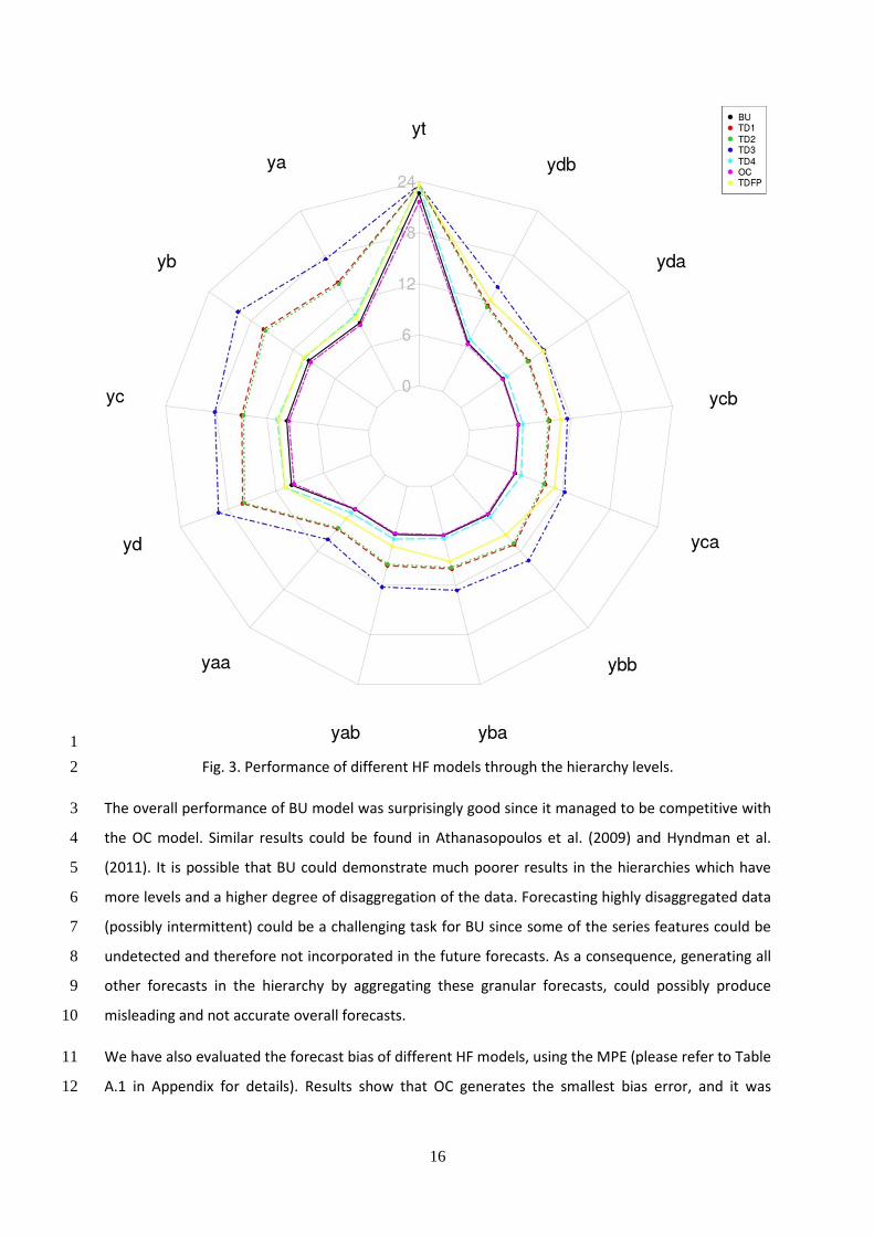
Fig. 3. Performance of different HF models through the hierarchy levels. 2

The overall performance of BU model was surprisingly good since it managed to be competitive with 3

the OC model. Similar results could be found in Athanasopoulos et al. (2009) and Hyndman et al. 4

(2011). It is possible that BU could demonstrate much poorer results in the hierarchies which have 5

more levels and a higher degree of disaggregation of the data. Forecasting highly disaggregated data 6

(possibly intermittent) could be a challenging task for BU since some of the series features could be 7

undetected and therefore not incorporated in the future forecasts. As a consequence, generating all 8

other forecasts in the hierarchy by aggregating these granular forecasts, could possibly produce 9

misleading and not accurate overall forecasts. 10

We have also evaluated the forecast bias of different HF models, using the MPE (please refer to Table 11

A.1 in Appendix for details). Results show that OC generates the smallest bias error, and it was 12

17

closely followed by the BU, TD4 and TDFP models. Conversely, TD1, TD2, TD3 underperformed and 1

generate highly biased forecasts (Fig. 4). 2

3 Fig. 4. MPE forecasting error of different models in the simulation study

j. 4

The Nemenyi post-hoc test failed to identify important differences between forecasts of all models, 5

except for TD3, for which test identified statistically different forecasts from other models. 6

Therefore, the main insights drawn from Table A.1 is aligned with Table 1. 7

4.2.2. Performance of the combination approaches 8

Bearing in the mind that several HF models may produce different outcomes (Table 1), combining 9

approaches may be the potential solution to improve the forecast accuracy. This recommendation is 10

usually given for individual (univariate) forecasting. We examine the combination of HF approaches 11

to see whether combining forecasts of HF models produces more accurate forecasts than using a 12

single HF model. 13

We examined various combinations of HF models in this research. However, we only present the 14

most accurate combination approach. The HF approaches present in the forecast combination 15

approaches are OC, BU and TD4. These models were top-performing individual HF models in Table 1. 16

The combination approaches are described in subsection 3.4. RMSEs and MPEs of the HF 17

combination models (COMB and COMBw) used in the simulation study are presented in the last two 18

columns of Tables 1 and A.1. 19

j The red line in a figure represents the median value of the MPE forecasting error of the OC model. Grey box

plots represent the performance of combined HF models (COMBw and COMB).

18

Fig. 2 displays the summarised performance of COMB and COMBw models (grey boxplots) compared 1

to other HF models. It indicates that combining the forecasts of OC, BU and TD4 reduces forecast 2

errors compared with any individual HF model. Moreover, it indicates that combinations have a thin 3

interquartile range, implying that COMB and COMBw generated reliable forecasts, which resulted in 4

stable forecasting errors through the entire hierarchy. Therefore, COMB and COMBw are robust and 5

consistent for generating forecasts across various hierarchies. 6

Overall, results show that the COMBw approach provides the most accurate forecasts on average. It 7

is calculated based on the simple average of RMSE across all levels. Moreover, the COMBw approach 8

outperforms all other HF approaches in all nodes of the hierarchy. COMBw was closely followed by 9

COMB, OC, BU and TD4 models. The accuracy of TD1, TD2, TD3 and TDFP was far behind the accuracy 10

of the COMB and COMBw models (Figs. 2 and 3). COMB and COMBw also presented good results in 11

terms of forecast bias but failed to outperform the OC, although the differences were not statistically 12

significant (Fig. 4). We observe that the forecast bias generated by COMB and COMBw approaches is 13

0.78% and 3.05% higher than the OC model, respectively (Table A.1). 14

4.2.3. Relative forecasting performance between competing models 15

From all individual approaches, OC model generates the most accurate forecasts in the simulation 16

study, with least bias (Tables 1 and A.1). Therefore, we use it as a benchmark to compare the 17

forecast accuracy improvement of other HF models and proposed combinations. To that end, we use 18

the average relative Mean Absolute Error (AvgRelMAE) proposed by Davydenko and Fildes (2013). In 19

order to determine improvement/reduction in forecasting performance between competing models, 20

AvgRelMAE uses a geometric mean of MAE ratios between models. The procedure of calculating 21

AvgRelMAE used in the paper is the following: 22

MN?O=PQM9 = RST01

0��U�/1

; T0 = QM90WQM90X .(12)

Where QM90X is the MAE of the baseline statistical forecast for the series i, QM90W is the MAE of the 23

competing model for the series i and m is the total number of time series. For a benchmark model, 24

we choose OC, which implies that QM90X = QM90-,. The results of the AvgRelMAE comparisons are 25

shown in Table 2. 26

Table 2. The AvgRelMAE forecasting performance of all HF models compared to the OC modelk. 27

k Best results are bolded.

19

Table 2 represents the increase or decrease of MAE forecasting error of different HF models, 1

compared to the forecasts of the OC model in every node. AvgRelMAE is easily interpretable, as it 2

represents the average relative value of MAE adequately, and directly shows how the observed 3

model improves/reduce the MAE compared to the baseline statistical forecast. Obtaining AvgRelMAE 4

< 1 means that on average MAE_ < MAEa, and therefore the observed model improves the accuracy, 5

while AvgRelMAE > 1 indicates the opposite (Davydenko & Fildes, 2013). 6

Results in Table 2 demonstrate that COMBw approach outperforms the OC and all other HF 7

approaches based on this metrics. COMBw generated consistently good forecasts, outperforming 8

other models in the majority of hierarchy nodes. For easier interpretation of overall forecasting 9

performance in terms of AvgRelMAE, we transform the last row of Table 2 to the percentage scale 10

(Tabel 3). The average percentage improvement in MAE of forecasts is found as (1 − AvgRelMAE) × 11

100. Positive values in Table 3 indicate the forecast improvement, while negative suggests the 12

opposite. Results demonstrate that by average COMBw reduces MAE forecasting error in the amount 13

of 1.66%, compared to the forecasts of the OC model. COMB and BU also show good results, but on 14

average they increase MAE forecasting error for the amount of 0.23% and 0.47%, respectively. All 15

other models generate forecasts that are significantly less accurate than forecasts of OC in each node 16

of the hierarchy. 17

Level Node AvgRelMAE

BU TD1 TD2 TD3 TD4 OC TDFP COMB COMBw

Level 0 Total 1.0470 1.0917 1.0917 1.0917 1.0917 1.0000 1.0917 1.0026 0.8781

Level 1

A 1.0163 1.5833 1.5614 1.8753 1.1247 1.0000 1.1252 1.0106 1.0063

B 1.0190 1.6408 1.6142 1.9612 1.1180 1.0000 1.1195 1.0051 1.0028

C 1.0181 1.5340 1.5116 1.8376 1.1245 1.0000 1.1222 1.0052 0.9972

D 1.0180 1.5805 1.5584 1.8670 1.1144 1.0000 1.1129 1.0047 0.9804

Level 2

AA 0.9919 1.4318 1.4061 1.6798 1.0797 1.0000 1.1969 1.0022 0.9992

AB 0.9953 1.4495 1.4283 1.7549 1.0919 1.0000 1.2035 1.0042 1.0006

BA 0.9937 1.4683 1.4421 1.7478 1.0778 1.0000 1.2240 0.9991 0.9935

BB 0.9970 1.5305 1.5046 1.8179 1.0799 1.0000 1.2273 0.9983 0.9903

CA 0.9898 1.4151 1.3900 1.7141 1.0731 1.0000 1.2296 0.9979 0.9861

CB 0.9887 1.4444 1.4194 1.6982 1.0822 1.0000 1.2572 0.9997 0.9855

DA 0.9897 1.4284 1.4049 1.7027 1.0813 1.0000 1.1908 0.9994 0.9816

DB 0.9967 1.5154 1.4898 1.7936 1.0853 1.0000 1.1986 1.0009 0.9815

Average 1.0047 1.4703 1.4479 1.7340 1.0942 1.0000 1.1769 1.0023 0.9833

20

Table 3. The average percentage improvement in MAE of all HF models compared to the OC modell. 1

Results in Figs. 2 and 3 supplemented with Tables 1, 2 and 3 indicate that combining the forecasts of 2

OC, BU and TD4 provides more accurate forecasts than any of individual HF models. In terms of 3

forecast bias, it appears that there is a still place for improvement of combination approaches since, 4

COMB and COMBw generated forecasts with higher bias, compared to the OC (Fig. 4 and Table A.1). 5

Overall, the results of a simulation study show that HF combinations could offer substantial benefit in 6

terms of HF forecasting. 7

5. EMPIRICAL EVALUATION 8

In Section 5, we assess the empirical validity of the main findings of this research using real time 9

series of a SC distribution network from a European brewery company. There is a lack of studies 10

evaluating the performance of the BU, TD and OC in the SCs. There are only a few examples linking 11

forecasting to various parts of SCs (Mircetic, 2018; Mircetic et al., 2017; Pennings & van Dalen, 2017; 12

Rostami-Tabar et al., 2015; Seongmin et al., 2012; Villegas & Pedregal, 2018). To the best of our 13

knowledge, this is the first study that examines a comprehensive grouped demand forecasting in a SC 14

network. The empirical study is performed to evaluate the effectiveness of different approaches in a 15

real SC network. Additionally, we also examine GF combinations in SC which has never been 16

investigated. 17

In subsection 5.1, we first provide details of the real SC distribution network and the empirical data 18

available for the purposes of our investigation along with the experimental structure employed in our 19

work. We then present the actual empirical results in subsection 5.2. 20

5.1. Supply chain distribution network 21

Fig. 5 illustrates a distribution structure of the brewery company operating in the South-East of 22

Europe. The scale economies in the transport of freight, combined with the market requirement to 23

provide fast and reliable delivery times, drive most large firms to operate multi-echelon distribution 24

inventories (Caplice & Sheffi, 2006). For the same reasons, the observed brewery company has a 25

multi-echelon distribution structure, and its distribution network spreads over several distribution 26

centers (DC) located across various geographical regions. Different DCs are designated to serve only 27

l Best results are bolded.

(1 − AvgRelMAE) × 100 (%)

BU TD1 TD2 TD3 TD4 OC TDFP COMB COMBw

Average -0.47 -47.02 -44.78 -73.39 -9.41 0.00 -17.68 -0.23 1.66

21

particular market regions. The distribution starts from the central warehouse, which is directly 1

connected to the manufacturing plant. The plant produces more than 200 different beer product 2

families. The annual output from the central warehouse varies, and it is usually between 250 000-300 3

000 pallets. Highest demand peaks occur in the spring/summer months (May, June and July) with the 4

demand picking to the 14 000 pallets of different brewery products. 5

6

Fig. 5. Multi-echelon brewery distribution network. 7

The brewery industry is specific in the sense that all of the consumption of the products is 8

accomplished via bars, restaurants and retail shops. There are no direct deliveries and internet sales 9

of products. In order to provide products to a wide consumer network, observed distribution chain is 10

divided into six marketing regions. These marketing regions are supplied through seven DCs. Each 11

region has one designated DC, except region 2, which is served through two DCs. Further distribution 12

of goods is carried out through wholesalers. There are four big wholesalers which are dominating in 13

the observed market. Some of those wholesalers are big retail chains, while others act as agents 14

between manufacturers and small retailers, bars and restaurants. Nevertheless, each wholesaler is 15

acquiring brewery products from the DCs and makes the further placement of goods on the market. 16

Goods that are provided to the wholesalers are classified as a brand and other products. Brand 17

products represent the most important products for the company since they are providing the 18

majority of revenue in the market. It is a top-selling beer which comes in different packaging types. In 19

observed brewery distribution chain, there is no further feedback from the wholesalers regarding the 20

point of sale data, therefore the visibility of the customer data is limited. 21

Main reasons for using the GF in SCs is to simplify forecasting process, obtain more accurate 22

forecasts, harmonise forecasts from different levels and to provide all information needed for 23

different SC parties. Therefore, in this empirical study, the forecasting structure is designed to 24

22

generate forecasts that support the planning and execution of the processes in different parts of SC. 1

Special attention is addressed to the alignment of the time component as well, and not just on the 2

cross-sectional alignment of the grouped structure. 3

5.2. Grouped structure for forecasting the brewery demand 4

The demand dataset available for the purpose of our research includes 56 weekly time series (SKUs) 5

for the period from 2012 to 2015; from a brewery company. The unit of observation is a pallet. The 6

demand in a given multi-echelon brewery distribution chain has the grouped structure. The structure 7

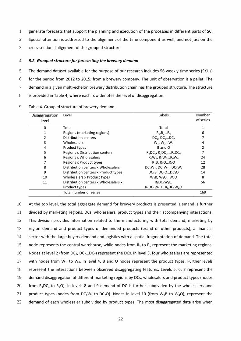
is provided in Table 4, where each row denotes the level of disaggregation. 8

Table 4. Grouped structure of brewery demand. 9

At the top level, the total aggregate demand for brewery products is presented. Demand is further 10

divided by marketing regions, DCs, wholesalers, product types and their accompanying interactions. 11

This division provides information related to the manufacturing with total demand, marketing by 12

region demand and product types of demanded products (brand or other products), a financial 13

sector with the large buyers demand and logistics with a spatial fragmentation of demand. The total 14

node represents the central warehouse, while nodes from R1 to R6 represent the marketing regions. 15

Nodes at level 2 (from DC1, DC2…DC7) represent the DCs. In level 3, four wholesalers are represented 16

with nodes from W1 to W4. In level 4, B and O nodes represent the product types. Further levels 17

represent the interactions between observed disaggregating features. Levels 5, 6, 7 represent the 18

demand disaggregation of different marketing regions by DCs, wholesalers and product types (nodes 19

from R1DC1 to R6O). In levels 8 and 9 demand of DC is further subdivided by the wholesalers and 20

product types (nodes from DC1W1 to DC7O). Nodes in level 10 (from W1B to W4O), represent the 21

demand of each wholesaler subdivided by product types. The most disaggregated data arise when 22

Disaggregation

level

Level Labels Number

of series

0 Total Total 1

1 Regions (marketing regions) R1,R2…R6 6

2 Distribution centers DC1, DC2…DC7 7

3 Wholesalers W1, W2…W4 4

4 Product types B and O 2

5 Regions x Distribution centers R1DC1, R2DC2,…R6DC6 7

6 Regions x Wholesalers R1W1, R1W2…R6W4 24

7 Regions x Product types R1B, R1O…R6O 12

8 Distribution centers x Wholesalers DC1W1, DC1W2…DC7W4 28

9 Distribution centers x Product types DC1B, DC1O…DC7O 14

10 Wholesalers x Product types W1B, W1O…W4O 8

11 Distribution centers x Wholesalers x

Product types

R1DC1W1B,

R1DC1W1O…R6DC7W4O

56

Total number of series 169

23

we consider the two product types that are supplied through seven different DCs to four different 1

wholesalers, giving a total of 2 x 7 x 4 = 56 bottom level series in the observed grouped structure. 2

These series represented by the nodes from R1DC1W1B to R6DC7W4O. Time plots of time series for the 3

first four levels are presented in Fig. 6. Results show that series are non-stationary, with a weak trend 4

and pronounced seasonality. 5

6

Fig. 6. Total weekly demand, disaggregated by marketing regions, DCs, wholesalers and product 7 types. 8

5.3. Data and empirical design of experiment 9

The forecast horizon is equal to the lead time of the decisions driven by the forecast. Since the 10

replenishment orders are required every week and manufacturing needs annual forecasts for 11

creating the production and procurement plan, the demand is forecasted on the weekly level for one 12

year ahead. All other sectors require forecasts between these two periods, so they can be easily 13

determined by looking at the forecasts for the period of their interest (monthly, quarterly, semi-14

annually and annually). 15

For evaluating the forecasting performance of HF/GF approaches using real time series, we divide 16

each series at each level into training/in-sample and test/out-of-sample sets. Training data is set to 17

104 weekly observations and includes the period from 2012 to 2014. The test data is set to 52 weekly 18

observations and it represents the period from 2014 to 2015. As in the simulation study, we also use 19

ETS forecasting models from forecast package in R, to produce out of sample base forecasts for the 20

brewery SC data. Forecasting horizon is set to 52-steps-ahead (one year ahead), and 1 to 52-steps-21

ahead forecasts are generated. After that, the out of sample error is determined for every series in 22

24

the grouped structure from Table 4. To report the forecast performance, we use RMSE, MPE and 1

AvgRelMAE performance metricsm

. 2

5.4. Empirical results 3

In this section, we present the results of the empirical investigation. In the subsection 5.4.1, we 4

jointly evaluate the effectiveness of GF approaches and GF forecast combinations using real data 5

from a brewery SC, while in the subsection 5.4.2 we examine whether GF forecast combinations 6

improve the forecast accuracy in terms of reducing the MAE, compared to the other competing 7

models. For forecasting the grouped brewery demand structure, we only keep BU and OC 8

approaches. We exclude TD approaches because of their unfeasibility with the empirical data 9

structure. Shang and Hyndman (2017) also suggest that BU and OC are the only approaches that are 10

currently suitable for forecasting the grouped demand structures. 11

5.4.1. The performance of the grouped forecasting approaches and its combinations 12

Results of the empirical study confirm the simulation results. Fig. 7 shows that all models produce 13

similar forecasts, compared by RMSE. 14

15

Fig. 7. Box plots for RMSEs of different models tested on the multi-echelon brewery distribution 16 chain

n. 17

We observe that the OC model performs slightly better than others followed by COMBw, COMB and 18

BU (please refer to Table A.2 in Appendix for details). However, its performance is not significantly 19

m Due to the space restrictions, we here only present RMSE, MPE and AvgRelMAE errors. Additional forecasting

error metrics (MAPE, MAE and ME), are also available from the corresponding author on request. n The red line in the figure represents the median value of the RMSE forecasting error of the OC model. Grey

box plots represent the performance of combined HF models (COMBw and COMB).

25

different from other three approaches, as the Nemenyi post-hoc test failed to identify important 1

discrepancy among forecasts of OC, COMBw, COMB and BU. 2

Fig. 8 presents the performance of BU, OC, COMB and COMBw approaches across all levels in the 3

forecasting structure presented in Table 4. It indicates that all approaches generate similar forecasts 4

in all levels and nodes of the forecasting structure. We develop a shiny platformo that allows users to 5

further compare and visualise the performance of these approaches through different forecasting 6

metrics, using real data from the multi-echelon brewery distribution chain. 7

8

Fig. 8. Performance of different models through the grouped levels while forecasting the demand in 9

the brewery distribution chainp. 10

o https://dejanmircetic.shinyapps.io/empirical_beverage_study/ p Numbers on the diagram perimeter represent the nodes in the grouped forecasting structure. To connect the

26

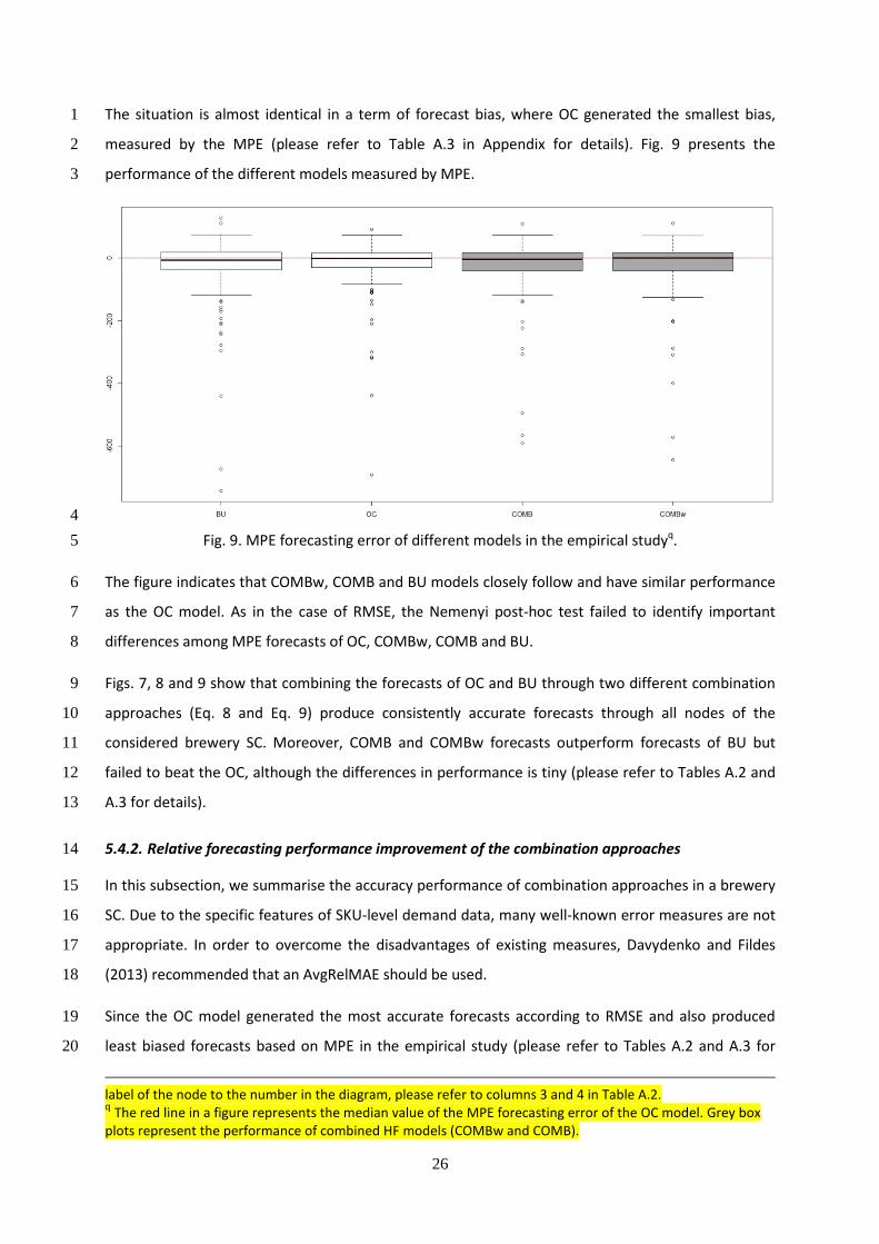
The situation is almost identical in a term of forecast bias, where OC generated the smallest bias, 1

measured by the MPE (please refer to Table A.3 in Appendix for details). Fig. 9 presents the 2

performance of the different models measured by MPE. 3

4

Fig. 9. MPE forecasting error of different models in the empirical studyq. 5

The figure indicates that COMBw, COMB and BU models closely follow and have similar performance 6

as the OC model. As in the case of RMSE, the Nemenyi post-hoc test failed to identify important 7

differences among MPE forecasts of OC, COMBw, COMB and BU. 8

Figs. 7, 8 and 9 show that combining the forecasts of OC and BU through two different combination 9

approaches (Eq. 8 and Eq. 9) produce consistently accurate forecasts through all nodes of the 10

considered brewery SC. Moreover, COMB and COMBw forecasts outperform forecasts of BU but 11

failed to beat the OC, although the differences in performance is tiny (please refer to Tables A.2 and 12

A.3 for details). 13

5.4.2. Relative forecasting performance improvement of the combination approaches 14

In this subsection, we summarise the accuracy performance of combination approaches in a brewery 15

SC. Due to the specific features of SKU-level demand data, many well-known error measures are not 16

appropriate. In order to overcome the disadvantages of existing measures, Davydenko and Fildes 17

(2013) recommended that an AvgRelMAE should be used. 18

Since the OC model generated the most accurate forecasts according to RMSE and also produced 19

least biased forecasts based on MPE in the empirical study (please refer to Tables A.2 and A.3 for 20

label of the node to the number in the diagram, please refer to columns 3 and 4 in Table A.2. q The red line in a figure represents the median value of the MPE forecasting error of the OC model. Grey box

plots represent the performance of combined HF models (COMBw and COMB).

27

details), we use it as a benchmark to compare the forecast accuracy improvement of BU and 1

proposed combination approaches (please refer Table A.4 in the Appendix for details). Table A.4 2

presents the increase or decrease of MAE forecasting error of different HF models, compared to the 3

forecasts of the OC model in the whole grouped brewery SC. 4

Results reveal that the OC model has outperformed others, generating the most accurate MAE 5

forecasts, although the Nemenyi post-hoc test failed to identify important differences between 6

models. COMBw and COMB generated consistently accurate forecasts in every node of the group 7

structure and had the closest performance to the OC model. BU also produce good forecasts but it 8

was outperformed by the OC, COMBw and COMB (Table 5). Table 5 presents the summarised 9

average percentage improvement in MAE of competing models, found as (1 − AvgRelMAE) × 100). 10

Table 5. The average percentage improvement in MAE of all GF models compared to the OC modelr. 11

Negative values in Table 5 indicate the reduction in forecast accuracy, compared to the OC model. 12

On average, COMBw and COMB generated approximately 0.5% higher MAE compared to the OC 13

model. BU forecasts were notably more inaccurate than forecasts of OC and on average produce 14

3.94% higher MAE errors than the OC model. Therefore, forecasts generated by the GF combinations 15

demonstrated accurate results and we recommend further development and usage of GF 16

combinations in contrast to using individual GF approaches to generate grouped time series forecasts 17

in SCs. 18

In this study, we have evaluated the performance of GF models via statistical metrics. The 19

performance of the forecasting methods should ideally be evaluated through utilities such as cost 20

reduction or service improvement. However, this is a challenging task as forecasting is used at 21

various levels of the hierarchy to support different type of decisions in Finance, logistics, marketing 22

or transportation planning. This will require the knowledge on how these functions are implemented 23

as well as their relevant monetary parameters. Moreover, evaluating the performance of GF models 24

on the entire hierarchical or grouped time series needs more research which we will be considered in 25

our future works. 26

r Best results are bolded.

(1 − AvgRelMAE) × 100 (%)

BU OC COMB COMBw

Average -3.9441 0.0000 -0.4961 -0.4908

28

6. THE EFFECT OF TIME SERIES CHARACTERISTICS ON THE PERFORMANCE OF FORECASTING 1

APPROACHES 2

In Section 4, we discuss that the performances of different models are increasingly diverging by 3

moving from the top aggregate level to the bottom level in the hierarchy. At the top level, all HF 4

models showed similar forecasts. In both studies (simulation and empirical), differences between 5

their performances become more apparent in the lower levels of the hierarchy, especially in the 6

bottom level. Therefore, we investigate whether there is any connection between the performance 7

of different HF models and characteristics of the series in the bottom level. 8

To the best of our knowledge, this is the first study that develops a model to evaluate the effect of 9

time series characteristics on the forecasting performance of different HF models. To that end, we 10

develop an additive multiple linear regression model. Multiple linear regression represents a model 11

for forecasting cross-sectional data. It assumes that there is a linear relationship between input 12

features X=(X1, X2,…,Xp), and the observed variable Y (Eq. 13). 13

b = c(d) + f. (13) 14

where f is a random error term, independent from X, with mean zero. It is the irreducible part of 15

forecasting error of the model, therefore we are only interested in estimating the relationship c(d) 16

shown in the Eq. 14. 17

b = g) + g�d� + g�d� + ⋯+ gidi + f. (14) 18

where d� represents the j predictor, and g� represents the average effect of d� predictor while 19

holding all other predictors fixed. 20

The algorithm provides insights into the interaction among characteristics of time series and the 21

accuracy of different HF models. The idea is to measure and extract different characteristics of time 22

series (that comprise the bottom level of the hierarchy), which will then be used as independent 23

features (X) in the multiple linear regressions. RMSEs of different HF models are set as dependent 24

variables (Y). The main goal is to identify the influential (i.e. statistically significant) time series 25

features, rather than creating the most accurate statistical learning algorithm on a given set of data. 26

For every HF model, a separate regression model was created. Therefore, we create seven regression 27

models. 28

This is the first research that investigates the impact of series characteristics and model performance 29

in the context of hierarchical forecasting. In this initial research, we are more interested in 30

developing a model that is easy to understand for managers than a complex one, which is hard to 31

29

interpret. Therefore, we put more emphasis on the model’s interpretability than on its predictive 1

power, i.e. we chose a simple linear model instead of complex nonlinear ones. There are no 2

restrictions in the settings that would limit the inclusion of complex nonlinear models as well, but it 3

will influence on model’s interpretability which is an important feature for the end-users. Generally, 4

if the aim is to develop an algorithm in which interpretability is not a concern, this research can be 5

easily extended to more flexible models, such as: Generalized additive models, Ridge regression, 6

Lasso regression, Classification and regression trees, Random Forests and Boosting trees. 7

For evaluating the statistical learning algorithm, we form a database which contains the results of the 8

simulation study. For each node in the bottom levels of the simulation study, 19 different time series 9

characteristics and RMSE forecast errors of HF models, are extracted, scaled and recorded in the 10

database. Therefore, the database contains 4000 different entries for time series measures and the 11

HF forecasting errors. We use 70% of the data for training and 30% for the test. Therefore, 19 12

different time series characteristics are used as independent variables in regression models which 13

are presented in the first column of Table 6 from number 1 to 19. 14

First, 16-time series characteristics are described in detail by Hyndman, Wang, and Laptev (2015) and 15

Wang, Smith-Miles, and Hyndman (2009). These characteristics might provide insights into why some 16

HF models perform better than others on the same data. We use given characteristics and added 17

additional three characteristics: i) correlation between observed bottom level series and the top 18

aggregate series (correlation (bts-top)); ii) the participation of observed series from the bottom level 19

to the top aggregate series (aggregate share); and iii) coefficient of variation. Additional 20

characteristics are calculated by the following equations: 21

C<TT=PFA><;(EAB − A<) = T� = ∑ k��,�'�l,�mmmmmn(��'��mmm)����o∑ k��,�'�l,�mmmmmn����� o∑ k��'��,mmmmn�����

; (15) 22

F??T=?FA=BℎFT= = ML� = ∑ ��,�����∑ ������ ; (16) 23

p<=cc>C>=;A<cNFT>FA><; = qr = o ��s� ∑ (��,�'��∑ ��,����� )�����

��∑ ��,����� . (17) 24

Where �t,�mmmm represents the mean value of observed j bottom level series (��,�) and ��u is the mean 25

value for the top level series (��), observed in the historical period t = 1,..., Т and j = 1, …, n. 26

The Coefficient of variation measures the volatility of the time series, while correlation (bts-top) is 27

measuring the strength and direction of the linear relationship amongst bottom level series and the 28

top aggregate series. Aggregate share measures the participation of the observed series from the 29

30

bottom level in top aggregate series. It provides the information about how “big” or “small” is 1

observed series in the given hierarchy. 2

Table 6. Summary statistics for the observed time series characteristics. 3

Table 6 provides the summary statistics for the time series characteristics that are used as input in 4

the statistical learning algorithms. Fig. A.1 in Appendix provides the distributions for the time series 5

characteristics. Distributions have different shapes, but the majority of the time series characteristics 6

have right-skewed distributions. 7

In order to determine the best subset of predictors, we use the best subset selection combined with 8

a validation test set (James, Witten, Hastie, & Tibshirani, 2013). The best subset selection procedure 9

is applied to the train data in order to determine the best model (i.e. combination of predictors) for 10

Time series

characteristics Mean

Standard

deviation Median Min Max Range Skew Kurtosis

1

Lumpiness (Variance

of annual variances of

remainder)

0.1072 0.1464 0.0525 0.0001 2.0815 2.0814 3.3441 20.3256

2 Entropy (Spectral

entropy) 0.8230 0.1531 0.8772 0.5378 0.9990 0.4612 -0.436 -1.3808

3 ACF1 (First order of

autocorrelation) 0.4536 0.4205 0.5491 -0.8612 0.9809 1.8421 -0.484 -1.0181

4 Lshift (Level shift) 0.9115 0.3358 0.8768 0.1635 1.9714 1.8079 0.3221 -0.7585

5 Vchange (Variance

change) 0.4028 0.1619 0.3937 0.0507 1.3470 1.2963 0.5684 0.8635

6 Cpoints (The number

of crossing points) 14.8788 10.5203 14.0000 1.0000 49.0000 48.0000 0.2970 -1.0800

7 Fspots (Flat spots) 5.3063 4.2595 4.0000 1.0000 39.0000 38.0000 2.4953 8.2992

8 Trend (Strength of

trend) 0.5771 0.3786 0.7216 0.0000 0.9985 0.9985 -0.341 -1.5784

9 Linearity (Strength of

linearity) -0.0084 3.9174 0.0012 -7.7978 7.6329 15.4306 0.0057 -0.7903

10 Curvature (Strength

of curvature) -0.0053 2.6101 -0.0361 -7.0502 6.9923 14.0424 0.0294 -0.0224

11 Spikiness (Strength of

spikiness) 0.0003 0.0007 0.0001 0.0000 0.0151 0.0151 5.3342 74.6329

12 Season (Strength of

seasonality) 0.4114 0.2293 0.4474 0.0000 0.9819 0.9819 -0.239 -0.9794

13 Peak (Strength of

peaks) 4.8182 4.1722 3.6155 0.0663 37.8018 37.7355 1.4785 3.1022

14 Trough (Strength of

trough) -4.7130 3.9976 -3.5012 -28.453 -0.0648 28.3889 -1.335 2.1290

15 KLscore (Kullback-

Leibler score) 1.2269 1.5811 0.7708 0.0702 41.7759 41.7057 8.7920 162.069

16

Change.idx (Index of

the maximum KL

score)

25.0863 11.6418 24.0000 12.0000 44.0000 32.0000 0.2237 -1.4699

17 Correlation (bts-top) 0.2367 0.4281 0.1781 -0.9174 0.9931 1.9105 -0.036 -0.5774

18 Aggregate share 0.1250 0.1215 0.0732 0.0080 0.7405 0.7325 1.6579 2.6632

19 Coefficient of

variation 0.8040 1.5286 0.2676 0.0065 14.1916 14.1851 3.8992 19.1592

31

each subset size (1 to 19 variables in the model). Following that, each model is elevated through the 1

validation test set. The model with the smallest test error (i.e. one that minimizes the mean square 2

error) is chosen as the most appropriate in the given situation. In order to obtain more accurate 3

estimates of the coefficients, best subset selection procedure is repeated on a whole data set and 4

previously determined optimal subset size. The final model is determined through evaluation of the 5

best model determined from the described selection procedure and the variance inflation factor 6

(VIF). VIF factor reveals the presence of possible multicollinearity in the predictors. As a rule of 7

thumb, a VIF value that exceeds 5 or 10 indicates a problematic amount of collinearity (James et al., 8

2013). Therefore, each model is tested on the presence of multicollinearity, and predictors with VIF 9

factor higher than 10 are excluded from the regression. The resulting models are presented in Table 10

7. 11

Table 7. The effect of time series characteristics on the performance of HF approaches. 12

In Table 7, coefficients are presented only when the effect of each time series characteristics is 13

statistically significant (p-value < 0.05)t. Each column represents a separate regression model created 14

s This is not a time series characteristic. It is the intercept of the regression model.

t We restrict extrapolation of the findings regarding the influence of time series characteristics on the

Time series characteristics BU TD1 TD2 TD3 TD4 OC TDFP

1 Intercepts 5.97 9.93 9.75 12.24 6.49 5.87 9.79

2 Lumpiness (Variance of annual

variances of remainder) 0.39 -4.36 -4.30 0.49 0.43

3 Entropy (Spectral entropy) 0.68 -6.39 0.67 0.75

4 ACF1 (First order of

autocorrelation)

5 Lshift (Level shift) 1.05 0.61 0.63 1.22 0.95

6 Vchange (Variance change) 0.57 -0.27 0.68 0.55

7 Cpoints (The number of crossing

points)

8 Fspots (Flat spots) 1.76 1.70 1.61

9 Trend (Strength of trend) 1.25 -1.06 -1.06 -0.83 1.09 1.23

10 Linearity (Strength of linearity) 0.53 0.85 0.79 1.03 0.49 0.48

11 Curvature (Strength of curvature) 0.54 0.53 0.52 0.29 0.54 0.55

12 Spikiness (Strength of spikiness) 0.33

13 Season (Strength of seasonality) -0.44 0.50 0.49 1.12 -0.34 -0.41

14 Peak (Strength of peaks) -0.38 0.11

15 Trough (Strength of trough) 0.37

16 KLscore (Kullback-Leibler score) -0.50 -0.48 -0.34

17 Change.idx (Index of the maximum

KL score) -0.62

18 Correlation (bts-top) 0.29 -1.93 -1.85 -2.46 0.35 0.31

19 Aggregate share 4.21 5.01 4.90 5.12 4.63 4.07 6.82

20 Coefficient of variation 0.47 0.84 0.84 0.53 0.50 0.46

Adjusted R2 0.6626 0.7546 0.7584 0.6855 0.5425 0.6565 0.015

32

for the different HF model. For different HF models, different characteristics found to be significant. 1

Table 7 shows that lumpiness Lshift, trend, linearity, curvature, season, correlation, aggregate share 2

and coefficient of variation are among time series characteristics that impact the performance of 3

majority HF models in the bottom level. Positive coefficients indicate that they contribute to the 4

increase of the forecasting error, while negative indicates the effect of decreasing the forecasting 5

error. Therefore HF models have a tendency of producing more inaccurate forecasts while 6

forecasting the time series with a higher values of Lshift, linearity, curvature, coefficient of variation 7

and aggregate share. 8

Other characteristics have a mixed influence on different HF models. Accordingly, lumpines, entropy, 9

Vchange, trend and correlation have an increasing effect on the accuracy of standard TD approachesu 10

(for those that it was significant), while for the majority of remaining HF models, they have a 11

decreasing effect on the accuracy. In contrast, higher values of season variable increase forecast 12

accuracy for the majority of HF models and decrease for standard TD approaches. Fspots and KLscore 13

have only a significant impact on the standard TD approaches, where Fspots decreases and KLscore 14

increases the forecasting accuracy. Other characteristics have less effect on the accuracy of HF 15

models and their effect in not holistic since they don't have statistically significant influence for the 16

majority of models. 17

The last row in Table 7 represents the adjusted R2, i.e. the percentage of the RMSEs variability of HF 18

error models explained by given additive linear regression models. The adjusted R2

ranges from 1.5% 19

of the explained error variability for the TDFP model, to the high 75.84% of the explained error 20

variability for TD2. 21

7. CONCLUSION AND FURTHER RESEARCH 22

Various levels of forecasts are required in SC to support decisions in different departments such as 23

logistics, marketing, manufacturing and finance. The current practice in SC is to generate separate 24

forecasts using univariate forecasting methodologies to support different decisions. Univariate 25

forecasting methodologies can only provide accurate forecasts for the unit for which forecasting is 26

performed such as particular level, sector or echelon in the SC. They are not able to provide coherent 27

forecasts across all levels or echelons of the SC. Consequently, these forecasts might be more 28

damaging for the efficiency of the SC, than having perhaps less accurate HF/GF forecasts that are 29

coherent across different parties of the SC. We argue that SC and HF/GF are naturally matched. In 30

forecasting performance, only on those time series which have similar or closely related summary statistics to

the data provided in Table 6 and Fig. A.1. u By standard TD approcses we mean TD1, TD2 and TD3 models.

33

this paper, we demonstrate the application of GF methodology in a multiple-echelon distribution 1

network of a major European brewery industry. Special emphasis is given to the design of the 2

forecasting structure to ensure that generated forecasts are aligned with the need of all parties 3

involved in delivering final products in the brewery distribution network. The forecasting structure 4

consists of eleven levels and 169 nodes in total. It provides forecasts for the planning and the 5

execution of processes in key parts of SC: manufacturing, marketing, finance, and logistics. 6

In this paper, we also considered the fact that there is no agreement on which HF approach provides 7

the most accurate forecast. Therefore, we evaluate the effectiveness of BU, TD and the OC 8

approaches in the simulation study, and examine whether a combination of these models improves 9

the forecast accuracy (COMB and COMBw). Moreover, we investigate the impact of time series 10

characteristics on the effectiveness of each HF approach. 11

The main findings of this paper can be summarised as follows: 12

• First, Optimal combination approach (with minimum trace estimator), following by BU 13

outperform all TD approaches on average and across all levels. Therefore, we recommend 14

practitioners to use these approaches when generating demand forecasts across various levels of 15

hierarchical or grouped data structures. Moreover, we notice that OC and BU approaches 16

demonstrate robustness and consistency in producing stable and accurate forecasts, regardless of 17

the hierarchy level and time series characteristics. This is a very important result for practitioners 18

as BU shows to be very competitive given its simplicity. 19

• Second, in comparing various variations of TD approaches, we observe that TD4 and TDFP 20

outperform other TD methodologies considered in this study. These approaches also seem to be 21

more robust to the hierarchy level and time series characteristics. 22

• Third, our results show that forecast combination of the existing BU, TD and OC models improve 23

the forecast accuracy. We propose two simple combination approaches based on existing models. 24

They are at least as accurate as forecasts generated by BU and OC approaches. Therefore, when 25

dealing with hierarchical and grouped demand structures in a SC, we recommend practitioners to 26

use a combination of models instead of using individual approaches. This is an important result 27

for practitioners as there is no concern about selecting the best method. 28

• Fourth, we examine the effect of time series characteristics on the forecasting performance of 29

different approaches at the bottom level of the hierarchy. The most influencing time series 30

characteristics on the accuracy of HF models are lumpiness Lshift, trend, linearity, curvature, 31

season, correlation, aggregate share and coefficient of variation. We also show that higher values 32

of the Lshift, linearity, curvature, coefficient of variation and aggregate share may have a negative 33

34

impact and deteriorate the forecast accuracy performance of HF models. Additionally, lumpiness, 1

entropy, Vchange, trend and correlation could have an increasing effect on the accuracy of 2

standard TD approaches (for those that it was significant), while for the majority of remaining HF 3

models they could contribute to decreasing of the forecasting accuracy. In contrast, higher 4

presence of the seasonality in data (season) may increase forecast accuracy for the majority of HF 5

models and decrease accuracy for standard TD approaches. Finally, Fspots and KLscore have only 6

a significant impact on the standard TD approaches, where Fspots could contribute to decreasing 7

and KLscore to increasing the forecasting accuracy. 8

• Finally, we demonstrate the application of grouped forecasting in SC using a multi-echelon 9

distribution network of a major European brewery company. We empirically present the holistic 10

approach for designing the forecasting structure while forecasting the demand in the SC. The 11

structure serves as the information platform to support the planning and execution of processes 12

in manufacturing, marketing, finances and logistics. 13

In order to guarantee the reproducibility principle in our research, we provide the R codes for the 14

simulation and empirical experiments used in this paper. Our codes will also be available in an open-15

source R package. 16

As far as the next steps of research are concerned, further work into the following areas would 17

appear to be merited: 18

• The interface between temporal and hierarchical or grouped aggregation has received minimal 19

attention in both academia and industry and this is an issue that we plan to investigate in the next 20

steps of our research. Creating a HF/GF methodology to produce the forecasts in the hierarchies 21

or grouped structures with horizontal connections between nodes within the same level is an 22

interesting avenue for further research. Current models can only produce forecasts in the 23

structures, which have vertical connections between nodes in different levels. These kind of 24

hierarchies or groups with horizontal and vertical connections are useful in the SC. 25

• The value of using exogenous variables in a hierarchical/grouped structure is an important avenue 26

for future research. The external variables that might be used in these structures might take three 27

forms: 1) variables that are independent of the aggregation level such as weather variable 2) 28

variables that are hierarchical in the same manner as the data such as population and 3) variables 29

that are independent or perhaps unique to each level such as GDP. Determining the conditions 30

under which causal models provide more accurate results and also which type of exogenous 31

variables should be used in a hierarchical structure has important implications in practice. 32

35

• The impact of time series characteristics from all levels in the forecasting structure and creating 1

an algorithm to link the time series characteristics of the entire forecasting structure to the 2

accuracy of each HF model is another interesting avenue for the future research. 3

• The extension of the work described here to cover utility metrics such as monetary savings would 4

allow linkage between forecasting and managerial decisions. Moreover, it may lead to new 5

methodologies to evaluate the forecast accuracy across a hierarchical structure. 6

7

REFERENCES 8

Aigner, D. J., & Goldfeld, S. M. (1973). Simulation and aggregation: a reconsideration. The Review of 9 Economics and Statistics, 114-118. 10

Athanasopoulos, G., Ahmed, R. A., & Hyndman, R. J. (2009). Hierarchical forecasts for Australian 11 domestic tourism. International Journal of Forecasting, 25(1), 146–166. 12

Babai, M. Z., Ali, M. M., & Nikolopoulos, K. (2012). Impact of temporal aggregation on stock control 13 performance of intermittent demand estimators: Empirical analysis. Omega, 40(6), 713-721. 14

Ballou, R. H. (2004). Business Logistics/Supply Chain Management-Planning, Organizing, and 15 Controlling the Supply Chain (Fifth edition ed.): Pearson/Prentice Hall. 16

Barnea, A., & Lakonishok, J. (1980). An analysis of the usefulness of disaggregated accounting data 17 for forecasts of corporate performance. Decision Sciences, 11(1), 17-26. 18

Boylan, J. (2010). Choosing levels of aggregation for supply chain forecasts. Foresight: The 19 International Journal of Applied Forecasting(18), 9-13. 20

Caplice, C., & Sheffi, Y. (2006). ESD.260J Logistics Systems. (Massachusetts Institute of 21 Technology: MIT OpenCourseWare), http://ocw.mit.edu. License: Creative Commons BY-NC-22 SA. 23

Chen, A., & Blue, J. (2010). Performance analysis of demand planning approaches for aggregating, 24 forecasting and disaggregating interrelated demands. International Journal of Production 25 Economics, 128(2), 586-602. 26

Chen, A., Yang, K., & Hsia, Z. (2008). Weighted least-square estimation of demand product mix and 27 its applications to semiconductor demand. International Journal of Production Research, 28 46(16), 4445-4462. 29

Chen, H., & Boylan, J. E. (2007). Use of individual and group seasonal indices in subaggregate 30 demand forecasting. Journal of the Operational Research Society, 58(12), 1660-1671. 31

Chopra, S., & Meindl, P. (2007). Supply chain management-Strategy, Planning, and Operation (3rd 32 ed.). New Jersey: Pearson Prentice Hall. 33

Collins, D. W. (1976). Predicting earnings with sub-entity data: Some further evidence. Journal of 34 Accounting Research, 163-177. 35

Dangerfield, B. J., & Morris, J. S. (1992). Top-down or bottom-up: Aggregate versus disaggregate 36 extrapolations. International Journal of Forecasting, 8(2), 233-241. 37

Davydenko, A., & Fildes, R. (2013). Measuring forecasting accuracy: The case of judgmental 38 adjustments to SKU-level demand forecasts. International Journal of Forecasting, 29(3), 510-39 522. 40

Dunn, D. M., Williams, W. H., & DeChaine, T. (1976). Aggregate versus subaggregate models in 41 local area forecasting. Journal of the American Statistical Association, 71(353), 68-71. 42

Dunn, D. M., Williams, W. H., & Spivey, W. A. (1971). Analysis and prediction of telephone demand 43 in local geographical areas. The Bell Journal of Economics and Management Science, 561-44 576. 45

Edwards, J. B., & Orcutt, G. H. (1969). Should aggregation prior to estimation be the rule? The 46 Review of Economics and Statistics, 409-420. 47

36

Fliedner, G. (1999). An investigation of aggregate variable time series forecast strategies with specific 1 subaggregate time series statistical correlation. Computers & Operations Research, 26(10), 2 1133-1149. 3

Fliedner, G. (2001). Hierarchical forecasting: issues and use guidelines. Industrial Management & 4 Data Systems, 101(1), 5-12. 5

Gordon, T. P., Morris, J. S., & Dangerfield, B. J. (1997). Top-down or bottom-up: Which is the best 6 approach to forecasting? The Journal of Business Forecasting, 16(3), 13. 7

Gross, C. W., & Sohl, J. E. (1990). Disaggregation methods to expedite product line forecasting. 8 Journal of Forecasting, 9(3), 233-254. 9

Grunfeld, Y., & Griliches, Z. (1960). Is aggregation necessarily bad? The Review of Economics and 10 Statistics, 1-13. 11

Hyndman, R. J., Ahmed, R. A., & Athanasopoulos, G. (2007). Optimal combination forecasts for 12 hierarchical time series. Department of Econometrics and Business Statistics. MONASH 13 University. Retrieved from http://www.buseco.monash.edu.au/depts/ebs/pubs/wpapers/ 14

Hyndman, R. J., Ahmed, R. A., Athanasopoulos, G., & Shang, H. L. (2011). Optimal combination 15 forecasts for hierarchical time series. Computational Statistics and Data Analysis, 55(9), 16 2579–2589. 17

Hyndman, R. J., & Athanasopoulos, G. (2014). Forecasting: principles and practice: OTexts. 18 Hyndman, R. J., & Athanasopoulos, G. (2018). Forecasting: principles and practice: OTexts. 19 Hyndman, R. J., Athanasopoulos, G., Bergmeir, C., Caceres, G., Chhay, L., O'Hara-Wild, M., . . . 20

Yasmeen, F. (2018). forecast: Forecasting functions for time series and linear models, R 21 package version 8.3. 22

Hyndman, R. J., Lee, A. J., & Wang, E. (2016). Fast computation of reconciled forecasts for 23 hierarchical and grouped time series. Computational Statistics & Data Analysis, 97, 16-32. 24

Hyndman, R. J., Wang, E., & Laptev, N. (2015). Large-scale unusual time series detection. Paper 25 presented at the Data Mining Workshop (ICDMW), 2015 IEEE International Conference on 26 IEEE. 27

James, G., Witten, D., Hastie, T., & Tibshirani, R. (2013). An introduction to statistical learning (Vol. 28 112): Springer. 29

Kahn, K. B. (1998). Revisiting top-down versus bottom-up forecasting. The Journal of Business 30 Forecasting, 17(2), 14. 31

Kinney, W. R. (1971). Predicting earnings: entity versus subentity data. Journal of Accounting 32 Research, 127-136. 33

Mircetic, D. (2018). Boosting the performance of top down methodology for forecasting in supply 34 chains via a new approach for determining disaggregating proportions. (Ph.D.), University of 35 Novi Sad, Serbia. 36

Mircetic, D., Nikolicic, S., Stojanovic, D., & Maslaric, M. (2017). Modified top down approach for 37 hierarchical forecasting in a beverage supply chain. Transportation research procedia, 22, 38 193-202. 39

Pennings, C. L., & van Dalen, J. (2017). Integrated hierarchical forecasting. European Journal of 40 Operational Research, 263(2), 412-418. 41

Pohlert, T. (2015). The pairwise multiple comparison of mean ranks package (PMCMR). 42 Rostami-Tabar, B. (2013). ARIMA demand forecasting by aggregation. Université Sciences et 43

Technologies-Bordeaux I. 44 Rostami-Tabar, B., Babai, M. Z., Ducq, Y., & Syntetos, A. (2015). Non-stationary demand forecasting 45

by cross-sectional aggregation. International Journal of Production Economics, 170, 297-309. 46 Schwarzkopf, A. B., Tersine, R. J., & Morris, J. S. (1988). Top-down versus bottom-up forecasting 47

strategies. The International Journal Of Production Research, 26(11), 1833-1843. 48 Seongmin, M., Hicks, C., & Simpson, A. (2012). The development of a hierarchical forecasting 49

method for predicting spare parts demand in the South Korean Navy—A case study. 50 International Journal of Production Economics, 140(2), 794-802. 51

Shang, H. L., & Hyndman, R. J. (2017). Grouped functional time series forecasting: An application to 52 age-specific mortality rates. Journal of Computational and Graphical Statistics, 26(2), 330-53 343. 54

37

Strijbosch, L. W. G., Heuts, R. M. J., & Moors, J. J. A. (2008). Hierarchical estimation as a basis for 1 hierarchical forecasting. IMA Journal of Management Mathematics, 19(2), 193-205. doi: 2 10.1093/imaman/dpm032 3

Syntetos, A., Babai, Z., Boylan, J., Kolassa, S., & Nikolopoulos, K. (2016). Supply chain forecasting: 4 Theory, practice, their gap and the future. European Journal of Operational Research, 252(1), 5 1-26. 6

Teunter, R. H., Babai, M. Z., Bokhorst, J. A., & Syntetos, A. A. (2018). Revisiting the value of 7 information sharing in two-stage supply chains. European Journal of Operational Research, 8 270(3), 1044-1052. 9

Trapero, J. R., Cardos, M., & Kourentzes, N. (2019). Empirical safety stock estimation based on 10 kernel and GARCH models. Omega, 84, 199-211. 11

Trapero, J. R., Kourentzes, N., & Fildes, R. (2012). Impact of information exchange on supplier 12 forecasting performance. Omega, 40(6), 738-747. 13

Turbide, D. (2015). How can distribution requirements planning help inventory management? 14 Retrieved 16.04.2016 15

Villegas, M. A., & Pedregal, D. J. (2018). Supply chain decision support systems based on a novel 16 hierarchical forecasting approach. Decision Support Systems, 114, 29-36. 17

Vogel, S. (2013). Demand fulfillment in multi-stage customer hierarchies: Springer Science & 18 Business Media. 19

Wang, X., Smith-Miles, K., & Hyndman, R. (2009). Rule induction for forecasting method selection: 20 Meta-learning the characteristics of univariate time series. Neurocomputing, 72(10-12), 2581-21 2594. 22

Weatherford, L. R., Kimes, S. E., & Scott, D. A. (2001). Forecasting for hotel revenue management: 23 Testing aggregation against disaggregation. Cornell hotel and restaurant administration 24 quarterly, 42(4), 53-64. 25

26

27