WORKING PAPER 215

Markus Knell

Actuarial Deductions for Early Retirement

The Working Paper series of the Oesterreichische Nationalbank is designed to disseminate and to provide a platform for Working Paper series of the Oesterreichische Nationalbank is designed to disseminate and to provide a platform for Working Paper series of the Oesterreichische Nationalbankdiscussion of either work of the staff of the OeNB economists or outside contributors on topics which are of special interest to the OeNB. To ensure the high quality of their content, the contributions are subjected to an international refereeing process. The opinions are strictly those of the authors and do in no way commit the OeNB.

The Working Papers are also available on our website (http://www.oenb.at) and they are indexed in RePEc (http://repec.org/).

Publisher and editor Oesterreichische Nationalbank Otto-Wagner-Platz 3, 1090 Vienna, AustriaPO Box 61, 1011 Vienna, Austriawww.oenb.atoenb.info@oenb.atPhone (+43-1) 40420-6666Fax (+43-1) 40420-046698

Editorial Board Doris Ritzberger-Grünwald, Ernest Gnan, Martin Summerof the Working Papers

Coordinating editor Coordinating editor Coordinating editor Martin Summer

Design Communications and Publications Division

DVR 0031577

ISSN 2310-5321 (Print)ISSN 2310-533X (Online)

© Oesterreichische Nationalbank, 2017. All rights reserved.

Actuarial Deductions for Early Retirement

Markus Knell∗

Oesterreichische Nationalbank

Economic Studies Division

October 2017

Abstract

The paper studies how the rates of deduction for early retirement have to be de-

termined in PAYG systems in order to keep their budget stable. I show that the

budget-neutral deductions depend on the specific rules of the pension system and

on the choice of the discount rate which itself depends on the collective retirement

behavior. For the commonly used fiction of a single individual deviating from the

target retirement age the right choice is the market interest rate while for the al-

ternative scenario of a stationary retirement distribution it is the internal rate of

return of the PAYG system. In this case the necessary budget-neutral deductions

are lower than under the standard approach used in the related literature. This

is also true for retirement ages that fluctuate randomly around a stationary distri-

bution. Long-run shifts (e.g. increases in the average retirement age) might cause

problems for the pension system but these have to be dealt with by the general

pension formulas not by the deduction rates.

Keywords: Pension System; Demographic Change; Financial Stability;

JEL-Classification: H55; J1; J18; J26

∗OeNB, Economic Studies Division, Otto-Wagner-Platz 3, POB-61, A-1011 Vienna; Phone: (++43-1)

40420 7218, Fax: (++43-1) 40420 7299, Email: Markus.Knell@oenb.at. The views expressed in this

paper do not necessarily reflect those of the Oesterreichische Nationalbank.

Non-Technical Summary

It is often argued that individuals should have a high degree of flexibility when choosing

their own retirement age. A crucial qualification to this statement, however, is that these

individual retirement decisions should be “budget-neutral”, i.e. they should leave the long-

run budget of the pension system unaffected. This paper studies how the budget-neutral

deductions for early retirement (and the budget-neural supplements for late retirement)

should be determined in order to meet this goal.

The paper shows that the level of these budget-neutral deduction rates depends on two

crucial factors: on the basic formulas of the pension system and on the assumption about

collective retirement behavior. As far as the pension formulas are concerned it makes a

difference whether the pension formula is independent of the retirement age (as is, e.g.,

the case for a pure defined benefit system) or whether it reacts rather strongly (as in a

notional defined contribution (NDC) system). The collective retirement behavior, on the

other hand, influences the discount rate that is used to calculate the present values of total

pension benefits and of total contributions which are needed to derive the budget-neutral

deduction rates.

In the paper it is shown that a NDC system will lead to a balanced budget without

the need of additional deductions or supplements if the retirement age is stationary. In

this case the costs of early retirement by some are exactly offset by the cost savings due

to late retirement of others. In a second step it is demonstrated that in this stationary

situation the appropriate discount rate is given by the internal rate of return (IRR) of the

PAYG system. This result stands in contrast to the related literature that often argues

that the use of the market interest rate is the necessary and almost self-evident choice to

determine budget-neutral deduction rates.

Various extensions confirm the main result of the paper. First, it is shown that a pure

NDC system without additional deductions is also able to guarantee an (approximately)

balanced budget when the actual retirement distribution fluctuates randomly around a

stable distribution. This constellation corresponds quite well to empirically observed pat-

terns. Second, I demonstrate that the main result (market interest rates are unimportant

for stationary retirement distributions) also holds for other PAYG systems (like defined

benefit systems or accrual rate systems). Third, I show that the use of unnecessarily

high deduction rates might also be compatible with a balanced budget but that it raises

fairness concerns. In particular, such a policy implies excessive punishments for early

retirement and excessive rewards for later retirement with probably unintended and un-

desired implications for the interpersonal distribution. Fourth, I discuss situations that

involve long-run shifts in demographic variables that might pose a challenge for PAYG

systems. I argue, however, that the appropriate reaction to these long-run changes have

to be factored into the basic pension formulas rather than into the deduction rates.

1 Introduction

This paper discusses how pay-as-you-go (PAYG) pension systems have to determine ac-

tuarial deductions for early retirement and actuarial supplements for late retirement in

order to remain financially balanced in the long run. Despite the fact that the levels of

deductions and supplements are crucial parameters for pension design that are present in

all real-world systems the existing literature on this issue is rather small and sometimes

controversial. In this paper I use a simple model to discuss this topic in a systematic and

comprehensive manner.

Deductions are necessary since an insured person who retires at an earlier age pays

less contributions into the pension system than an otherwise identical individual and he

or she also receives more installments of (monthly or annual) pension payments.1 The

deductions have to be determined in such a way that the net present value of these altered

payment streams is zero. This calculation depends on two crucial factors. The first one is

the definition of the pension formula. Many pension systems take the difference between

the actual retirement age R and the target (or “statutory”) retirement age R∗ into account

when assigning the pension payment. The stronger pension benefits react to the difference

between the actual and the target age the weaker the need for additional deductions. In

the paper I focus on three variants of PAYG systems: a defined benefit (DB) system that

does not react to the actual retirement age R; an accrual rate (AR) system (as it is,

e.g., in place in Germany or France) where the basic pension formula already implies a

lower pension payment for earlier retirement; and a notional defined contribution (NDC)

system (introduced in countries like Sweden, Italy or Poland) which is based on a formula

that adjusts pension payments to the fact that early retirement is associated with fewer

years of contributions and with more years of pension payments.

The second important factor to calculate budget-neutral deductions is the discount

rate that is used to equalize the present value of costs and benefits. In the related

literature the most common suggestion is to use the market interest rate. This is, e.g.,

argued by Werding (2007, p.21) on the grounds that the “government has to borrow the

funds for premature pensions” and that the relevant interest rate for these transactions

is “evidently the capital market interest rate”, in particular the “risk-less interest rate

for long-run government bonds”. In the present paper I argue that this choice is not

1From now on I will focus on the case of early retirement and the associated deductions. All of thefollowing statements and results, however, also hold for the opposite case of late retirement and associatedsupplements.

1

as self-evident as suggested in the related literature. In fact, the level of discount rates

that is appropriate to calculate budget-neutral deduction rates depends on the collective

retirement behavior. The standard approach of the literature uses a thought experiment in

which everybody retires at the target retirement age R∗ while only one individual retires at

an earlier age. In this hypothetical scenario the behavior of the deviant individual causes

an extra financing need and the market interest rate is in fact the appropriate concept for

discounting the ensuing cash flows. Early retirement can, however, not only occur in the

context of such a one-time-shock scenario. There exists, e.g., also an alternative scenario

where people retire at different ages according to a retirement distribution that is stable

over time. It is not clear from the outset whether the conventional wisdom also holds for

this alternative assumption about collective behavior.

In this paper I look at this issue in detail. The main result of the analysis consists

of two parts. First, I show that if the retirement ages follow a stationary distribution

over time then a NDC system leads to a stable budget. The costs of early retirement are

exactly offset by cost savings of late retirement and there is no financial need for additional

deductions or supplements. Second, in this case the appropriate discount rate is given by

the internal rate of return (IRR) of the PAYG system. Contrary to wide-spread claims

in the literature, it is thus not necessary or “evident” to use the market interest rate for

the determination of budget-neutral deductions. The rest of the paper adds elaborations,

extensions and discussions of the central result.

First, I show that it is straightforward to amend the two other PAYG systems (DB

and AR) in order to “mimic” the NDC system. It is thus sufficient to derive and discuss

the main results for the NDC system since they can be easily extended to the other pen-

sion formulas. Second, for illustrative purposes I calculate deduction rates for realistic

demographic scenarios. For a discount rate that equals the IRR of the PAYG system the

deductions are between 5.5% and 7.0% (DB system) and 4.2% and 4.9% (AR system)

while they are 0% for the NDC system. The use of higher discounts rates increases the

annual deduction rates by slightly less than 1:1. In particular, for an interest rate that

is 2% higher than the internal rate of return they range from 7.3% to 8.7% (for the DB

system), 5.7% to 6.6% (for the AR system) and 1.8% to 1.9% (for the NDC system).

Third, given the fact that different discount rates imply different deductions it is crucial

to choose the appropriate assumption concerning collective retirement behavior. I discuss

this issue and argue that there exist good reasons to regard the stationary retirement

distribution as the more reasonable reference point. On the one hand, the one-time shock

scenario cannot be extended over time. In the year after the single early retiree left the

2

labor market the initial situation has changed and it is no longer appropriate to start

with the thought experiment in which everybody retires at the target age. If every period

a certain fraction of individuals retire early than one would ultimately end up with the

other scenario of a stationary distribution. On the other hand, real-world retirement pat-

terns do not correspond to such a degenerate distribution where almost everybody retires

at the target age, but show a wider, rather stable and typically slowly changing distri-

bution. Fourth, I look at various additional scenarios where the retirement age follows

a non-stationary distribution. Also in many of these cases the appropriate deductions

are below the value that are associated with the one-time-shock scenario. In particular,

numerical simulations show that for situations where the actual retirement distributions

fluctuate randomly around a stable distribution a pure NDC system is basically sufficient

to guarantee a balanced budget and the additional deductions can be close to zero. Fifth,

I demonstrate that even for a stationary distribution of retirement ages the choice of a

higher discount rate might still be associated with a balanced budget if the target retire-

ment age R∗ is equal to the average actual retirement age. If this is not the case then the

system will run permanent surpluses or deficits. The use of a higher discount rate is how-

ever not innocuous in both situations. In particular, it might look problematic from the

viewpoint of the interpersonal distribution since it implies that early retirees have to pay

deductions that are larger than what is necessary for budgetary stability while late retirees

are offered larger-than-necessary supplements. Sixth, I briefly discuss various extensions

of the model. In the first extension I generalize the basic model with rectangular mortal-

ity to a model with an arbitrary mortality structure. The main results continue to hold

in this framework. Further extensions deal with additional heterogeneity along various

dimensions and with pension systems that are unbalanced by construction. For the as-

sumption of a stationary retirement distribution it is still the case in these extensions that

the level of budget-neutral deductions is related to the IRR of the system and independent

of the market interest rates. The deduction rates, however, might now have distributional

consequences. Finally, I discuss situations that involve long-run shifts in demographic or

economic variables that often pose a challenge for PAYG systems. An increase in the

average retirement age, e.g., leads to a constellation where none of the common deduction

rates (neither the one based on market interest rates nor the one based on the IRR) is

able to implement a balanced budget. These long-run changes have to be reflected in the

design of the basic pension formulas and they require more thorough considerations about

intergenerational risk-sharing and redistribution. These difficult issues have to be treated

separately from the more modest topic of how to determine budget-neutral deduction

3

rates.

There exists a broad literature on actuarial adjustments from the perspective of

the insured individuals. This is sometimes called the “microeconomic” or “incentive-

compatible” viewpoint (cf. Borsch-Supan 2004, Queisser & Whitehouse 2006) since it

focuses on the determination of deductions that leave an individual indifferent between

retiring at the target or at an alternative age. This individual perspective has been used to

study the impact of non-actuarial adjustments on early retirement (Stock & Wise 1990,

Gruber & Wise 2000), the incentives to delay retirement (Coile et al. 2002, Shoven &

Slavov 2014) and the simultaneous decisions on retirement, benefit claiming and retire-

ment in structural life cycle models (Gustman & Steinmeier 2015). The present paper

concentrates on the “macroeconomic viewpoint”, i.e. on actuarial adjustments from the

perspective of the pension system.2 The literature on this topic is smaller than the one on

incentive-compatibility. Queisser & Whitehouse (2006) offer terminological discussions

and they present evidence on the observed rates of adjustments. For a sample of 18

OECD countries they report an average annual deduction for early retirement of 5.1%

and an average annual supplement of 6.2% for late retirement. They conclude that “most

of the schemes analysed fall short of actuarial neutrality [and that] as a result they sub-

sidize early retirement and penalize late retirement” (p.29). An intensive debate about

this topic can be observed in Germany where the rather low annual deductions rates of

3.6% are frequently challenged. A number of researchers have supported higher rates

of deductions based on market interest rates (Borsch-Supan & Schnabel 1998, Fenge &

Pestieau 2005, Werding 2007, Brunner & Hoffmann 2010) while other participants have

argued for keeping rates low stressing the lower IRR of the PAYG system (Ohsmann

et al. 2003). Overviews of the debate can be found in Borsch-Supan (2004) and Gasche

(2012).

The paper is organized as follows. In section 2 I present the basic deduction equation

and I focus on a simple model that allows for analytical solutions. In section 3 I derive the

level of budget-neutral deductions for various assumptions concerning collective retirement

behavior. In section 4 I discuss the case of “excessive deductions”, i.e. of deductions that

are higher than necessary for budgetary balance which might raise distributional concerns.

2“Actuarial neutrality” (either of the microeconomic or of the macroeconomic type) must also bedistinguished from the notion of “actuarial fairness”. The latter concept is often used to describe asystem in which the present value of expected contributions is ex-ante equal to the present value ofexpected pension payments (cf. Borsch-Supan 2004, Queisser & Whitehouse 2006). This is therefore alife-cycle concept while actuarial neutrality can be regarded as a “marginal concept” that focuses on theeffect of postponing retirement by an additional year.

4

Section 5 and 6 discuss various extensions and section 7 concludes.

2 Simple framework

2.1 Set-up

I start with the benchmark approach of the related literature. In order to fix ideas I focus

on the most simple case with a constant wage W and a stable demographic structure

where all individuals start to work at age A, are continuously employed and die at age

ω.3

There exists a PAYG pension system with a constant contribution rate τ , a target (or

reference) retirement age R∗ and a pension formula that determines the regular pension

for each admissible retirement age R. In the most simple form the system only determines

the pension level P ∗ that is promised for a retirement at the target age R∗. In this case

the pension deductions are the only instrument to implement appropriate adjustments

for early retirement. Many real-world pension systems, however, are based on a “formula

pension” that depends on the target retirement age R∗ and on the actual retirement age

R thereby accounting (at least partially) for early retirement. This formula pension is

denoted by P (R,R∗) and I will discuss below various possibilities for its determination.

For the moment, however, I leave it unspecified. Furthermore, for brevity I will often omit

the arguments of P (R,R∗) and other functions whenever there is no risk of ambiguity.

Finally, the pension level at the target retirement age is given by P ∗ ≡ P (R∗, R∗).

2.2 Deductions for a general discount rate

If an individual chooses to retire before the target age (i.e. R < R∗) then the actuarial

neutral deduction for early retirement will reduce the formula pension payment P in such

a way that the retirement decision has no long-run effect on the budget of the social

security system. In order to do so two effects have to be taken into account. First, for the

periods between R and R∗ the individual does not pay pension contributions and thus

the system has a shortfall of revenues. Second, in these periods of early retirement the

individual already receives pension payments and thus the system has to cover additional

expenditures. The formula pension level P thus has to be reduced by a factor X (that is

3In appendix C I will discuss the case where wages grow at rate g(t) and where there exists mortalitybefore the maximum age ω.

5

valid for the entire pension period) in order to counterbalance these two effects. The final

pension will thus be given by P = PX. Using a continuous time framework the actuarial

deduction factor X is implicitly defined as follows:∫ R∗

R

(τW + PX

)e−δ(a−R) da =

∫ ω

R∗

(P ∗ − PX

)e−δ(a−R) da, (1)

where δ is the social discount rate used to evaluate future payment streams. The left-hand

side of equation (1) contains the twofold costs to the system due to early retirement (i.e.

the period loss of contributions τWand the additional period expenditures PX). The

right-hand side captures the benefits to the system since in the case of a retirement at the

target age the pension without deductions would be P ∗ for all periods between R∗ and ω

which is now reduced to P = PX.4

The determination of the discount rate δ is a crucial issue. In fact, it will turn out that

different approaches to calculate appropriate deductions differ primarily in their choice

of the discount rate (see also Gasche 2012). If the costs of early retirement have to be

financed by debt then the market interest rate seems to be the right choice, i.e. δ = r. If,

one the other hand, the budget of the system remains under control (e.g. because early

retirement of some is counterbalanced by late retirement of others) then a lower interest

rate like the internal rate of return of the PAYG system seems appropriate. I come back

to this crucial issue later.

One can solve equation (1) for X which gives rise to a rather complicated expression.

Linearization of this result (around δ = 0) leads to the approximated value X given by:

X =ω −R∗

ω −R

[P ∗

P+τW

P

R−R∗

ω −R∗+δ

2(R−R∗)

(P ∗

P+τW

P

)]. (2)

4The same logic also holds for late retirement with R > R∗. In this case the equivalent to (1) is

given by:∫ RR

∗(τW + P ∗) e−δ(a−R) da =

∫ ωR

(PX − P ∗

)e−δ(a−R) da. This can be transformed to yield

(1). Note that equation (1) could also be viewed as the condition that makes an individual indifferentbetween retirement at the age of R∗ and retirement at an earlier age R. In this case the appropriatediscount rate is given by his or her individual rate of time preference which is typically associated withthe market interest rate. The deductions derived under this approach are sometimes termed “incentivecompatible”. They could also be called “actuarial neutral from the perspective of the insured person”.A related concept is the “social security wealth” that is often used in this context to study the incentivesfor early or delayed retirement (see e.g. Stock & Wise 1990, Gruber & Wise 2000, Shoven & Slavov 2014).In the present I focus, however, on “budget neutral” deductions which could also be called “actuarialneutral from the perspective of the insuring system”.

6

2.3 Different PAYG systems

In order to further evaluate expression (2) and to derive numerical values one has to

specify how the formula pension level P is determined. There exist various possibilities

and I will discuss three variants that are often used in existing pension systems.

• Defined Benefit (DB) System: In this case there exists a target replacement

rate q∗ that is promised if an individual retires at the target retirement age R∗. In

the generic DB case the pension formula is independent of the actual retirement age

and does not reduce the target replacement rate, i.e. PDB(R,R∗) = q∗W .

• Accrual Rate (AR) System: Many countries have PAYG pensions systems in

place that are somewhat more sensitive to actual retirement behavior than the DB

system. In particular, in these systems the formula pension is reduced if retirement

happens before the target age R∗. One popular example of such a system is built

on the concept of an “accrual rate”. For each period of work the individual earns

an accrual rate κ∗ that is specified in a way that the system promises the full

replacement rate q∗ only if the individual retires at the target retirement age R = R∗.

This means that κ∗ = q∗ 1R∗−A and PAR(R,R∗) = κ∗(R− A)W = q∗ R−A

R∗−AW .5

• Notional Defined Contribution (NDC) System: This scheme has been estab-

lished in Sweden and in a number of other countries and is increasingly popular.

Its main principle is that at the moment of retirement at age R the total of con-

tributions that an individual has accumulated over the working life τW (R − A) is

transformed into a period pension by dividing it by the remaining life expectancy

ω−R. This means that PNDC(R,R∗) = τW R−Aω−R .6 Therefore in the NDC system the

target retirement age R∗ does not play a role and the formula pension just reacts

to the actual retirement age R.

The pension for early (or late) retirement in each of the three cases j ∈ {DB,AR,NDC}is then given by Pj = PjXj (where I skip again the function values). I call the ratio of

the final pension Pj to the target pension P ∗j the total pension reduction. This reduction

might be either due to stipulations of the formula pension Pj or due to the influence of

the explicit deductions Xj. For the DB system, e.g., the entire reduction follows from the

5A system like that is, e.g., in place in Austria. The earnings point system in Germany or France canalso be directly related to this PAYG variant.

6Real-world NDC systems are more complicated due to non-stationary economic and demographicpatterns. This is discussed in appendix C.

7

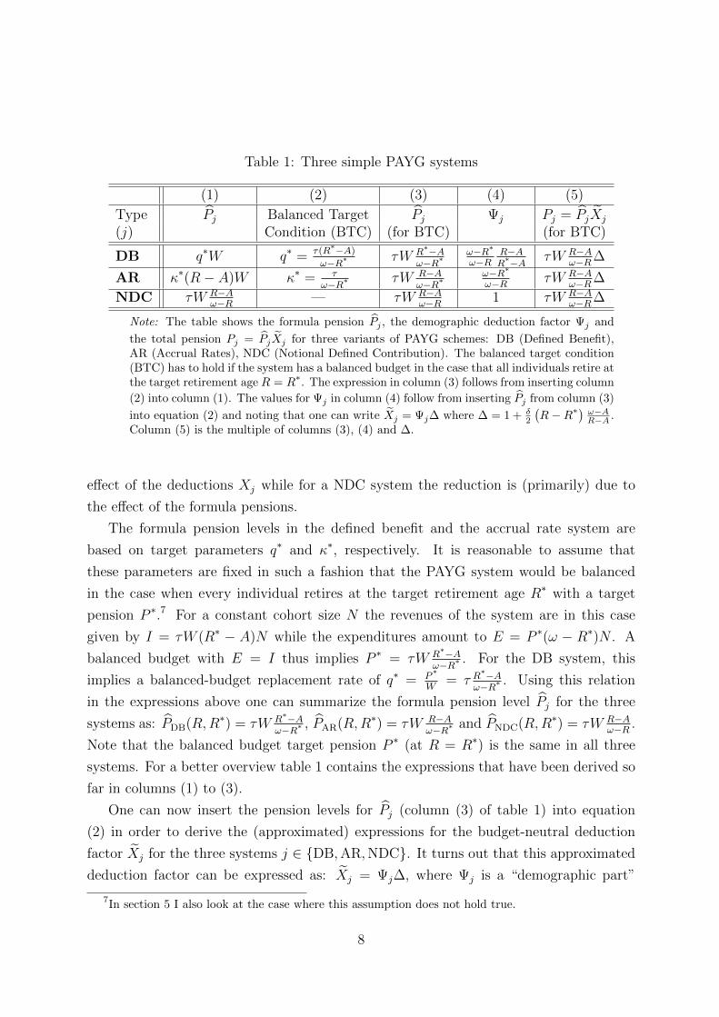
Table 1: Three simple PAYG systems

(1) (2) (3) (4) (5)

Type Pj Balanced Target Pj Ψj Pj = PjXj

(j) Condition (BTC) (for BTC) (for BTC)

DB q∗W q∗ = τ(R∗−A)

ω−R∗ τW R∗−A

ω−R∗ω−R∗ω−R

R−AR∗−A τW R−A

ω−R∆

AR κ∗(R− A)W κ∗ = τω−R∗ τW R−A

ω−R∗ω−R∗ω−R τW R−A

ω−R∆

NDC τW R−Aω−R — τW R−A

ω−R 1 τW R−Aω−R∆

Note: The table shows the formula pension Pj , the demographic deduction factor Ψj and

the total pension Pj = PjXj for three variants of PAYG schemes: DB (Defined Benefit),AR (Accrual Rates), NDC (Notional Defined Contribution). The balanced target condition(BTC) has to hold if the system has a balanced budget in the case that all individuals retire atthe target retirement age R = R∗. The expression in column (3) follows from inserting column

(2) into column (1). The values for Ψj in column (4) follow from inserting Pj from column (3)

into equation (2) and noting that one can write Xj = Ψj∆ where ∆ = 1 + δ2

(R−R∗) ω−A

R−A .Column (5) is the multiple of columns (3), (4) and ∆.

effect of the deductions Xj while for a NDC system the reduction is (primarily) due to

the effect of the formula pensions.

The formula pension levels in the defined benefit and the accrual rate system are

based on target parameters q∗ and κ∗, respectively. It is reasonable to assume that

these parameters are fixed in such a fashion that the PAYG system would be balanced

in the case when every individual retires at the target retirement age R∗ with a target

pension P ∗.7 For a constant cohort size N the revenues of the system are in this case

given by I = τW (R∗ − A)N while the expenditures amount to E = P ∗(ω − R∗)N . A

balanced budget with E = I thus implies P ∗ = τW R∗−A

ω−R∗ . For the DB system, this

implies a balanced-budget replacement rate of q∗ = P∗

W= τ R

∗−Aω−R∗ . Using this relation

in the expressions above one can summarize the formula pension level Pj for the three

systems as: PDB(R,R∗) = τW R∗−A

ω−R∗ , PAR(R,R∗) = τW R−Aω−R∗ and PNDC(R,R∗) = τW R−A

ω−R .

Note that the balanced budget target pension P ∗ (at R = R∗) is the same in all three

systems. For a better overview table 1 contains the expressions that have been derived so

far in columns (1) to (3).

One can now insert the pension levels for Pj (column (3) of table 1) into equation

(2) in order to derive the (approximated) expressions for the budget-neutral deduction

factor Xj for the three systems j ∈ {DB,AR,NDC}. It turns out that this approximated

deduction factor can be expressed as: Xj = Ψj∆, where Ψj is a “demographic part”

7In section 5 I also look at the case where this assumption does not hold true.

8

that just depends on the demographic and economic variables ω, A, R and R∗, while ∆

is a “financing” part that also depends on the discount rate δ.8 In particular, ΨDB =ω−R∗ω−R

R−AR∗−A , ΨAR = ω−R∗

ω−R , ΨNDC = 1 and ∆ = 1 + δ2

(R−R∗) ω−AR−A . These results are

collected in column (4) of table 1. Column (5) shows that the application of the deduction

factor Xj leads to an identical final pension payment Pj for all three systems.

2.4 Deductions for different discount rates

One can now look at the deductions for various assumptions of the discount rate. At the

moment I am not concerned about the budgetary implications of this choice and I am just

focusing on the level of deductions that follow from the exact Xj (see equation (1)) or the

approximated Xj (see (2)). In the literature one can find two benchmark assumptions

concerning the discount rate which will be discussed below. As a first possibility it is

assumed that δ = r, i.e. the discount rate is set equal to the market interest rate. As a

second possibility it is argued that the social discount rate should be set to the internal

rate of return of a PAYG pension system. In the simple example of this section without

economic or population growth the internal rate of return is zero and thus δ = 0. In fact,

it is straightforward to show that for a growing economy with W (t) = W (0)egt and where

ongoing pensions are adjusted with the growth rate g equation (2) is unchanged except

that now δ has to be substituted by the “net discount rate” δ ≡ δ − g.

The assumption δ = 0 (or δ = 0) is a natural starting point which implies that ∆ = 1

and also XNDC = XNDC = 1. The basic formula of the NDC system PNDC = PNDC =

τW R−Aω−R is thus enough to implement the required reduction for early retirement that

fullfills the neutrality condition (1). This is different for the two other variants where

the pension formula does not suffice to stipulate the necessary reductions even though

∆ = 1. In particular, the additional deduction has to be such that the final pension is

exactly equal to PNDC = τW R−Aω−R . For the case of the accrual rate system this means that

XAR = ω−R∗ω−R while for the DB system one gets that XDB = ω−R∗

ω−RR−AR∗−A .

For a positive discount rate δ > 0, however, even a NDC system will not lead to

long-run stabilization. It is useful to illustrate the magnitude of these effects for realistic

numerical values. In particular, assume that people start to work at the age of A = 20,

that they die at the age of ω = 80, that the contribution rate is τ = 0.25, the target

retirement age R∗ = 65 and the constant wage W = 100. In tables 2 and 3 I show the

8The two coefficients are functions of the various variables, i.e. Ψj = Ψj(R,R∗, ω,A) and ∆ =

∆(R,R∗, ω,A, δ). For better readability I again leave out the function arguments.

9

Table 2: Deductions for R = 64 and R∗ = 65

δ = 0 δ = 0.02 δ = 0.05

Type j Pj Xj xj(in%) Pj Xj xj(in%) Pj Xj xj(in%) PjDB 75.00 0.92 -8.33 68.75 0.90 -9.64 67.77 0.88 -11.81 66.14AR 73.33 0.94 -6.25 68.75 0.92 -7.59 67.77 0.90 -9.80 66.14NDC 68.75 1 0 68.75 0.99 -1.43 67.77 0.96 -3.79 66.14

Note: The table shows the actuarial deduction factors Xj , the annual deductions rates xj (based on the

linear relation xj =Xj−1

R∗−R ) and the final pension Pj(R,R

∗) = Pj(R,R∗)Xj for three pension schemes

and three discount rates. The numerical values are: A = 20, ω = 80, τ = 0.25, W = 100, R∗ = 65 andR = 64. All cohort members are assumed to reach the maximum age (rectangular survivorship).

Table 3: Deductions for R = 60 and R∗ = 65

δ = 0 δ = 0.02 δ = 0.05

Type j Pj Xj xj(in%) Pj Xj xj(in%) Pj Xj xj(in%) PjDB 75.00 0.67 -6.67 50. 0.62 -7.70 46.13 0.53 -9.33 40.01AR 66.67 0.75 -5.00 50. 0.69 -6.16 46.13 0.60 -8.00 40.01NDC 50.00 1. 0. 50. 0.92 -1.55 46.13 0.80 -4.00 40.01

Note: The table shows the actuarial deduction factors Xj , the annual deductions rates xj (based

on the linear relation xj =Xj−1

R∗−R ) and the final pension Pj(R,R

∗) = Pj(R,R∗)Xj for three pension

schemes and three discount rates. The numerical values are: A = 20, ω = 80, τ = 0.25, W = 100,R∗ = 65 and R = 60. All cohort members are assumed to reach the maximum age (rectangularsurvivorship).

magnitude of the necessary budget-neutral deductions for the case of R = 64 (R = 60)

and three values of the discount rate δ (0%, 2% and 5%).9 In order to transform the total

deduction factor X into an annual (or rather period) deduction rate x there exist two

possibilities. As one possibility one can use the continuous-time framework to conclude

from X = ex(R∗−R) that x = ln(X)

R∗−R . In existing pension systems, however, the period

deductions are typically expressed in a linear way, i.e. x = X−1R∗−R . In the following tables

I show the period deduction rates (in %) based on this linear formula.

All three systems promise a pension of P (R∗, R∗) = 75 for a retirement at age R∗ = 65.

For early retirement at R = 64 the formula pension is reduced to PNDC(R,R∗) = 68.75

9The numbers show Xj , i.e. the exact solutions to equation (1) and not Xj of the approximatedformula (2). The quantitative differences between these two magnitudes are, however, small.

10

for the NDC system which is the actuarial amount as long as δ = 0. For the accrual rate

system, on the other hand, the formula pension is only reduced to PAR(R,R∗) = 73.33

and the system thus needs additional deductions in order to guarantee stability. For the

current example the necessary annual deduction rate is 6.25%. For the traditional DB

system the annual deduction rate is even larger (8.33%) since there is no adjustment of

the pension PDB(R,R∗). For discount rates above 0 also the NDC needs extra deductions.

For δ = 0.02, e.g., the annual deductions are 1.43% and for δ = 0.05 they are 3.79%. For

the DB and the AR system the annual deductions also increase by an amount that is

somewhat smaller than the extent of δ. If one looks at the even earlier retirement at age

R = 60 (see table 3) then the results are qualitatively similar. Now the NDC pension is

only 50 instead of 75 (for δ = 0) and for the other two systems the annual deductions are

somewhat smaller than before.10

Summing up, one can conclude that the levels of actuarial deductions depend both on

the exact pension formula and on the choice of the social discount rate. For δ = 0 the

basic formula of the NDC system is sufficient and no additional deductions are necessary.

For the DB and AR systems, however, even for δ = 0 one needs deductions that depend on

the demographic structure and on the rules of the pension system. These “demographic

deduction factors” are sizable (for our numerical examples between 5% and 8%) and

typically larger than the additional deductions that are necessary if one chooses a positive

discount rate. In appendix C I show that these conclusions remain valid in a more general

framework.

3 Budget-neutral deductions

In the previous sections I have discussed the rates of deduction for different values of

the discount rate without looking at the budgetary implications of the various choices.

In this section I focus on the appropriate choice to implement a PAYG system that

runs a balanced budget. “Budgetary neutrality” requires that retirement before and

after the target retirement age does not have an effect on the budget of the pension

system in the long run. This requirement implies that one has to consider the collective

retirement behavior in order to be able to evaluate the budgetary consequences. The look

10This is due to the fact that the deductions now have more time to take force and therefore theannual deductions can be smaller. For the same reason it also holds that supplements for late retirement(e.g. R = 66, results not shown) are larger than the corresponding deductions for early retirement (e.g.R = 64). There is less time to reap the benefits of later retirement and therefore the period supplementshave to be higher.

11

at individual retirement decisions is not sufficient since early retirement of one group might

be accompanied by late retirement of another group such that the average retirement age

stays unchanged. Furthermore, even if the average retirement age in a certain period

is below the target age this might still be counterbalanced by higher average retirement

ages in later periods. The assessment of budgetary neutrality is thus impossible without

the consideration of the intratemporal and intertemporal distribution of retirement ages.

Deductions (over and above the demographic part) are only needed insofar as the system

has to take out loans in order to finance additional expenditures. If the system can use the

intra- and intertemporal variations to provide the necessary funds then these additional

financing needs can be reduced or completely avoided.

In the following I discuss this issue for a number of interesting cases. In the first case

the distribution of retirement ages is assumed to be stationary over time. For this case it

can be shown that a NDC system is always balanced. Since there are no extra financing

needs this finding corresponds to an implicit discount rate of δ = 0. In the second case it

is assumed that everybody retires at the target age and only one individual of one cohort

at a lower age. This one-time-shock scenario represents the simplest example of a non-

stationary retirement distribution and is the benchmark case of the related literature. I

derive that in this case the correct choice of the discount rate is given by δ = r. In a third

section I look at various other non-stationary distributions and calculate the appropriate

actuarial deductions for these situations. All examples have in common that they start

from a specific distribution and return to the same distribution after an intermezzo of

non-stationary periods. It will appear that for many of these situations the actuarial

deduction rates are considerably lower than the values of the one-time-shock scenario and

often close to zero.11

3.1 Set-up and budget

In order to calculate the level of budget-neutral deductions the natural first step is to the

define the budget of the pension system. I stick to the simplified model of the previous

section, i.e. to a model in continuous time with the assumption of rectangular survivorship

where all members of a cohort reach the maximum age ω. The wage is fixed at W and

the contribution rate at τ . In appendix C it is shown that the main results also hold

in a model with a growing wage level and with an explicit mortality structure. In every

11A separate issue is the case where the distribution of retirement ages (and in particular the averageretirement age) shifts over time. The discussion of this case is postponed to section 6.2.

12

instant of time a cohort of equal size N is born. The length of the working life (and

thus the number of contribution periods) depends on the starting age and the retirement

age. For sake of simplicity I assume that all individuals start to work at age A and are

continuously employed up to their individual retirement age R. For the latter I assume

that the age-specific probability to retire for generation t is given by f(a, t) for a ∈ [A, ω].

The cumulative function F (a, t) indicates the fraction of cohort t that is already retired

at age a. It holds that F (A, t) = 0 and F (ω, t) = 1. In the simple model of this section

retirement fluctuations are the only possible source of non-stationarity.

The total (adult) population Q(t) is constant and given by:

Q(t) = N(ω − A). (3)

The size of the retired population M(t) can be derived from the following considerations.

For a given retirement age R there are individuals of ages a ∈ [R,ω] that are in retirement.

Their relative frequencies are given by f(R, t−a).12 Integrating over all possible retirement

ages R ∈ [A, ω] leads to:

M(t) = N

∫ ω

A

(∫ ω

R

f(R, t− a) da

)dR. (4)

The total size of the active population L(t) can be calculated as:

L(t) = Q(t)−M(t) = N

[(ω − A)−

∫ ω

A

(∫ ω

R

f(R, t− a) da

)dR

]. (5)

Turing to the budget of the system, total revenues I(t) are given by:

I(t) = τW (t)L(t). (6)

Total expenditures E(t), on the other hand, can be written as:

E(t) = N

∫ ω

A

(∫ ω

R

P (R, a, t− a)f(R, t− a) da

)dR, (7)

where P (R, a, t − a) stands for the pension payment of a member of cohort t − a. The

size of the pension can depend on the payment period t, on the individual’s age a and

12Note that f(R, s) denotes the retirement density of the cohort born in period s. In period t the massof individuals who retired at age R and are now a years old is therefore given by f(R, t− a).

13

also on the time of his or her retirement R ≤ a. As in the previous section the pension

P is the product of the formula pension P and the deduction factor χ. In particular,

one can write Pj(R, a, t − a) = Pj(R, a, t − a)χj(R, a, t − a) for j ∈ {AR,DB,NDC}.Both the formula pension and the deduction factor might depend on t, a and R. In

the following I will concentrate on the NDC system since the other two systems can

be transformed into the NDC scheme easily by the use of the demographic adjustment

factors ΨAR and ΨDB as shown in section 2. For the sake of readability I leave out the

subscript “NDC” in the following and thus write P (R, a, t−a) = P (R) = τW R−Aω−R . In the

following the deduction factor thus refers to the NDC system. In principle, this deduction

factor χ(R, a, t − a) might differ with respect to time, age and the retirement age. One

could, e.g., have a deduction factor that changes from period to period in reaction to

the general budgetary outlook. This would be similar to the ABM (Automatic Balance

Mechanism) in the Swedish system. Alternatively one might have a situation where the

deduction factor is not calculated once and for all at the moment of retirement but changes

during the retirement years. This possible age- and time-dependence will of course have

implications for the intra- and intergenerational distribution. I abstract from these issues

here, however, and focus on deduction factors that are independent of time and age and

only differ with respect to the retirement age, i.e. χ(R, a, t − a) = X(R). For the NDC

system (where the demographic part of the deduction factor is given by Ψ = 1) one can

write X(R) = (1 + x(R − R∗)) where x is the time-invariant deduction rate. This is the

specification that is employed in the related literature and that also corresponds to the

design of real-world deduction rates. One should nevertheless bear in mind that one could

also use different and more elaborate specifications for χ(R, a, t− a).

The deficit in period t is defined as:

D(t) = E(t)− I(t) (8)

and the deficit ratio as:

d(t) =D(t)

I(t)=E(t)

I(t)− 1. (9)

A balanced budget in period t thus requires D(t) = 0 or d(t) = 0. The intertemporal

balanced budget constraint between some periods t0 and tT , on the other hand, reads as:∫ tT

t0

D(t)e−r(t−t0)dt = 0, (10)

14

where r is the capital market interest rate that has to be used to finance possible budgetary

shortfalls (or at which possible surpluses can be invested). Budget-neutral deductions can

then be defined as the value of x such that equation (10) is fulfilled.13

In the following I will discuss a number of cases and investigate how the budget-neutral

deduction rate x depends on the assumption concerning the collective retirement behavior

as captured by the density functions f(R, t).

3.2 Case 1: A stationary distribution of retirement ages

I start with the natural benchmark case of a stationary retirement distribution, i.e.

f(R, t) = f(R) and F (R, t) = F (R). The main result is summarized in the following

proposition.

Proposition 1

Assume a situation with a constant wage rate W , a constant cohort size N , a constant

entry age A, a constant longevity ω, rectangular mortality and a retirement age that is

distributed according to the density function f(R) for R ∈ [A, ω]. In this case a NDC sys-

tem will be in continuous balance (D(t) = 0,∀t) without the need of additional deductions

(X(R) = 1 or x = 0).

Proof. In order to see this I first assume that the proposition is correct (i.e. x = 0) and

then show that this in fact leads to a balanced budget with D(t) = 0. To do so one can

insert the NDC pension P (R) = τW R−Aω−R (assuming x = 0) into (7) which leads to

E(t) = N

∫ ω

A

(∫ ω

R

τWR− Aω −R

f(R) da

)dR

= τWN

∫ ω

A

(R− A)f(R) dR = τWN(R− A),

where R ≡∫ ωARf(R) dR stands for the average retirement age. This is the same as total

revenues since

I(t) = τWL(t) = τWN

[(ω − A)−

∫ ω

A

(∫ ω

R

f(R) da

)dR

]= τWN

[(ω − A)− (ω −R)

]= τWN(R− A) = E(t).�

13If the period-by-period balancing condition D(t) = 0,∀t were used instead of the intertemporalbalanced budget condition (10) one would need a time-varying deduction factor χ(R, t− a) (or possiblyχ(R, a, t− a)) in order to guarantee the balanced budget.

15

For a stationary distribution of retirement ages f(R) a pure NDC system is thus

balanced in every period (D(t) = 0,∀t). There is no need for loans to finance the early

retirement of some individuals, the capital market interest rate is irrelevant and extra

deductions are unnecessary (x = 0). Using the results of section 2 (see table 1) this

also implies that the appropriate discount rate for the standard deduction equation (1) is

δ = 0.

The intuition behind this result is straightforward. The system needs money to finance

the pension of the early retirees with a RL < R. This is available, however, since in

the previous periods the early retirees did not get the full pension that would be paid

for retirement at the average age R (i.e. P = τW R−Aω−R ) but rather the smaller pension

P = τW RL−A

ω−RL. A similar argument holds for the late retirees where their higher pension

can be financed by the extra contributions of the late retirees of future generations.

3.3 Case 2: A one-time shock in retirement ages

This case is dominant in the related literature on actuarial deductions (Borsch-Supan

2004, Werding 2007, Gasche 2012). In particular, the situation is based on the thought

experiment that everybody retires at the target retirement age R∗ except one individual

who chooses a lower retirement age.14 To be more precise, I assume that there is a small

mass θ of members of cohort t who retire at RL < R∗. All other individuals retire at the

target age. The question is how to choose the deduction factor X(RL) (or the deduction

rate x) such that the intertemporal budget condition (10) (∫ tTt0D(t)e−r(t−t0)dt = 0) is

fulfilled (for t0 < t < tT − ω).

The first thing to note is that in all periods before t + RL the deficit is balanced.

From periods (t+RL) to (t+R∗) the revenues of the system are lower than normal due

to the early retirement of the deviating group of mass θ. For these periods the deficit

D(t) is further increased due to the fact that the early retirees already receive a pension

payment PL = PLX(RL) = τW RL−A

ω−RLX(RL) which would not be the case had they stayed

employed until the target retirement age R∗. On the other hand, the expenditures of the

system are lower than normal for the time periods between (t + R∗) and (t + ω) due to

the fact that the pension of the early retirees is lower than the target pension. After the

early retirees have died in period (t+ ω) the pension system is back to the normal mode

with a continuous balance of D(t) = 0. The intertemporal budget condition (10) only

14In fact, it is not necessary that everybody retires at the target age but only that everybody retiresat the same age.

16

involves non-zero values for these exceptional periods and can thus be written as:

θ

∫ t+R∗

t+RLτWe−r(t−(t+R

L)) dt+ θ

∫ t+R∗

t+RLPLX(RL)e−r(t−(t+R

L)) dt

−θ∫ t+ω

t+R∗

(P ∗ − PLX(RL)

)e−r(t−(t+R

L)) dt = 0.

Choosing t = 0 and canceling θ one can observe that this is exactly the same expression

as the standard deduction equation (1) with the choice of a discount rate δ = r. The

necessary deduction factor is then given by the formula in (2), i.e. by X(RL) = ∆ =

1 + r2

(RL −R∗

)ω−ARL−A

(see table 1).

In this one-time-shock scenario the size of the interest rate has an impact on the

budget-neutral deduction rate since the pension system has to take out a loan at the

interest rate r > 0 in order to deal with the financial consequences of the early retirement

decisions.15

3.4 Case 3: Further non-stationary distributions of retirement

ages

Case 2 is the simplest case of a non-stationary distribution. It is based, however, on

a highly stylized scenario and it would be misleading to neglect other, arguably more

plausible scenarios. In the following I discuss two examples.

Two-point distribution For non-stationary patterns of retirement it is typically not

possible to derive analytical solutions and one has to revert to numerical simulations.

There exists, however, one particularly simple distribution that can be solved analytically

and is thus useful to fix ideas. In particular, assume that up to cohort t each individual

either chooses a low retirement age RL1 or a high age RH

1 , with relative frequencies p1 and

(1−p1), respectively. The average retirement age per cohort is thus given by R1 = p1RL1 +

(1−p1)RH1 . From cohort t on there is a shift in retirement behavior and now a fraction p2

retires at age RL2 > RL

1 and a fraction (1−p2) at age RH2 < RH

1 . The aggregate retirement

age per cohort, however, is assumed to stay the same, thus R2 = p2RL2 +(1−p2)RH

2 = R1.

The system is balanced before period t+RL1 and after period t+ ω but in-between there

will be a number of periods with budget surpluses and deficits.

15This is, e.g., the argument used by Werding (2007) to justify the use of market interest rates tocalculate budget-neutral deductions.

17

In particular, the early retirees of cohort t retire later than the early retirees of previous

cohorts (RL2 > RL

1 ). This means that the system has a number of periods with higher

revenues and lower expenditures in which it runs a surplus. On the other hand, later on

there will be periods with a larger number of retirees than before due to the fact that

the late retirees leave the labor market sooner (RH2 < RH

1 ). In these periods the system

will face more expenditures, less revenues and will thus run a deficit. The challenge is

to choose a deduction rate x such that the present value of the sum of these surpluses

and deficits is zero, i.e. such that the intertemporal balanced budget condition (10) is

fulfilled. This budget-neutral deduction rate will clearly depend on the size of the interest

rate r. In appendix A I show that in the case with r = 0 and x = 0 the present value

D =∫ t+ωt+R

L1D(t)e−r(t−(t+R

L1 ))dt comes out as D = 1

2τWN(R1 − R2)(ω − A). Since in the

example I have assumed that R1 = R2 it follows that D = 0 and thus with r = 0 and

x = 0 the surpluses and deficits just offset each other. For positive values of r this is,

however, no longer true and one needs a non-zero deduction rate x. For example, with

τ = 0.25, W = 100 and RL1 = 60, RH

1 = 70, RL2 = 65, RH

2 = 65, p1 = p2 = 12

and thus

R1 = R2 = 65 one can calculate that x = −0.0057 (for r = 0.02) and x = −0.014 (for

r = 0.05). These deduction rates are thus larger than in the benchmark NDC case (where

x = 0) but also considerably smaller than the standard deductions based on equation (1)

where they come out as x = −0.0133 (for r = 0.02) and x = −0.0333 (for r = 0.05). The

use of these larger deduction rates would lead to a permanent surplus of the system

The one-time shift in the two-point distribution is, however, again a rather special

case of a non-stationary development. There exist at least two reasons why it is not a

particularly useful benchmark for realistic scenarios. First, the retirement ages follow a

deterministic process and second the average retirement age of all retirees does not stay

constant (for the example above it increases from 63.3 to 65). The following stochastic

example does not suffer from either of these problems.

Random fluctuations: In order to study more complicated non-stationary distribu-

tions one has to revert to numerical simulations in a discrete-time framework, since an-

alytical solutions are no longer possible. Appendix B contains a detailed description of

the discrete-time model. As a benchmark scenario I look at a situation where the cohort-

specific retirement densities f(R, t) are random draws from a stable distribution f ∗(R). In

the appendix I discuss the results of an example where this stable retirement distribution

is triangular between the ages 60 and 70 with a mean at R = 65 that is also the target age

R∗. The parameters of the simulation are chosen in such a way that fluctuations in the

18

retirement age roughly correspond to real-world data. For each simulation I calculate the

deduction rate x that solves the discrete-time equivalent of equation (10) and I verify that

this value manages to keep the budget in balance. Figure A.2 in the appendix illustrates

this for one specific simulation. Over one-hundred simulation runs the average of these

budget-neutral deduction rates x is close to zero. In particular, it comes out as x = 0.0002

with a standard deviation of 0.003.

This shows that the result of proposition 1 also holds approximately true for time-

variant retirement distributions. A pure NDC system with only minimal additional de-

ductions will be compatible with a stable long-run budget as long as the retirement ages

fluctuate around a stationary target distribution.16

3.5 Summary

In this section I have used various examples to emphasize a crucial point: the level of

budget-neutral deductions depends on the assumptions concerning the collective retire-

ment behavior. For a stationary retirement distribution the formula pension of a standard

NDC system is sufficient to guarantee a balanced budget and there is no need for addi-

tional deduction. This corresponds to the choice of a discount rate δ = 0 in the commonly

used equation (1). For the often used thought experiment of a one-time-shock there are

additional financing needs and the formula pension has to be amended by a deduction

rate that follows from equation (1) by setting δ = r. Both of these benchmark scenarios

are arguably rather stylized. Neither do policymakers face a population with a completely

stationary retirement behavior nor do they observe only a few individuals that deviate

from the statutory retirement age. In fact, the second scenario is not an ultimately con-

vincing benchmark case since it cannot be extended over time. In the year after the single

early retiree left the labor market there will no longer be a situation where all individu-

als have an identical retirement age (which has been the initial situation of the thought

experiment). One could assume that a constant fraction of each cohort chooses the early

retirement age but this would then correspond to the alternative situation of a retirement

distribution that is stationary over time. If one looks at empirical data (see appendix B)

then it seems to be the case that—absent radical policy reforms—the retirement distribu-

tion is rather constant and changes only slowly over time. The scenario of a stable target

distribution with random fluctuations around this distribution thus seems to be a better

16In fact, setting x = 0 from the beginning and calculating the revenues and expenditures for the 100simulation runs also leads to a budget that is (almost) balanced on average, however with a considerablylarger standard deviation of budgetary outcomes across the different simulations.

19

approximation of real-world behavior. The results of section 3.4 then suggest that the use

of a NDC system without additional deductions (x = 0) will guarantee an approximately

balanced budget in this situation.

The entire discussion so far has, however, been built on the assumption that there are

no long-run shifts in retirement behavior like an increase in average retirement age. In

section 6 I will come back to this issue. I will argue that cases with long-run shifts are

certainly not unrealistic but that the deduction rates are the wrong parameter to deal

with this phenomenon.

4 Excessive deductions

Even though a deduction rate of x = 0 (with a corresponding discount rate δ = 0) is

sufficient for a stable budget in the case of stationarity (see proposition 1) it is nevertheless

interesting to look at a situation where despite this fact the system chooses an additional

deduction rate x < 0 (or a positive discount rate δ > 0). In order to study this in more

detail one can use the expression from section 2 for the NDC-pension given in column (5)

of table 1:

P = P X = τWR− Aω −R

(1 +

δ

2(R−R∗) ω − A

R− A

). (11)

Inserting this expression together with the assumed stationary retirement density f(R)

into equation (7) leads to total expenditures E(t) = τWN(R− A+ δ

2(ω − A)(R−R∗)

).

Total revenues (6), on the other hand, are given by I(t) = τWN(R − A). From this one

can calculate the deficit as

D(t) = τWNδ

2(ω − A)

(R−R∗

). (12)

Equation (12) confirms the results from above that the budget of the system with a

stationary retirement distribution is in permanent balance if one chooses a discount rate

of δ = 0. For the case of a positive discount rate δ > 0 one has to distinguish between

two cases. If the target retirement age R∗ is set equal to the average actual retirement

age R then the budget of the system is still in balance, while for R∗ 6= R this is no longer

true. The implications of these two cases are studied in the following.

Balanced budget with higher deductions Equation (12) implies that a positive

discount rate is still compatible with a permanently balanced budget as long as R∗ = R.

20

The positive discount rate is, however, not necessary for budgetary reasons since the

balance would materialize for any value of δ. This means that the higher pensions for the

later retirees are paid by the deduction of the early retirees. Whether this is a reasonable

and fair property depends on the preferences and the objectives of the system. If, e.g.,

the main reason for early retirement is seen as a preference for leisure and if (for whatever

reason) the policy-makers strive for a higher average retirement age it looks defendable

to implement such an unnecessary scheme of intragenerational redistribution. If, on the

other hand, early retirement is due to bad health or harsh working conditions it might

be deemed unfair that those individuals get an additional punishment for their early

retirement by paying for the augmented pensions of their more fortunate peers.

Permanent deficits or surpluses with higher deductions An even more severe

deviation from the benchmark case with δ = 0 occurs if the discount rate is positive and

the target retirement age is set above the average retirement age (R∗ > R). In this case

equation (12) indicates that the budget will show a permanent surplus (D(t) < 0) while

there will be a permanent deficit (D(t) > 0) in the reverse case (R∗ < R). To give a

numerical example set A = 20, ω = 80, R∗ = 65 and R = 63. If the social planner

chooses a discount rate of δ = 0.05 then the deficit ratio d(t) ≡ D(t)/I(t) comes out

as d(t) = −0.07. This means that every period the expenditures are 7% lower than the

revenues and the system is permanently in surplus.

It is not straightforward to decide whether a situation with a permanent surplus or a

permanent deficit is reasonable. In order to do so one would need to specify the optimal

size of the PAYG pension system which depends—inter alia—on individual and social

preferences, on the economic environment and also on the history of the system. Such

an analysis is beyond the scope of the present paper. In fact, in the framework of the

simple model presented so far there exists no prima facie reason for a PAYG system since

a funded pension system with r > g (where in the simple model g = 0) will provide a

higher rate of return that does not have to be weighted against potentially higher risk (due

to the assumption of complete certainty). In reality, however, the rationale behind the

introduction of a PAYG system is typically based on concerns about myopic behavior,

intergenerational smoothing, poverty prevention and risk-sharing. As a short-cut one

could assume that these concerns have been taken into account in the original design of the

PAYG pillar and that the optimal (i.e. socially preferred) size of the system corresponds

to the actual revenues at the time of its introduction, i.e. to I(0) = τWN(R−A). In this

case, however, it would not make sense to choose a target level R∗ > R and a deduction

21

δ > 0 since this would lead to a permanent surplus and thus to a shrinkage of the PAYG

system as compared to its optimal size. In particular, the pension for R∗ > R and δ > 0

would be lower for individuals with R < R∗ than for the benchmark case with δ = 0. The

early retirees would thus pay for the partial dismantling of the PAYG system. They are

treated like the transition generations after the abolishment of a PAYG system who also

have to contribute twice (once for the public pension system and once for their private

savings).

These are not academic reflections in the framework of a stylized model but they form

the background of regular and sometimes rather heated debates on the appropriate level

of deductions in many countries. In Germany, some authors have argued for considerably

higher deduction rates than the current value of 3.6% in order to implement an incentive-

compatible scheme (Borsch-Supan & Schnabel 1998, Borsch-Supan 2004, Werding 2007).

Others have countered that it is problematic on normative grounds to choose deductions

that are higher than required for budget neutrality just in order to achieve general political

goals (Ohsmann et al. 2003).

5 Extensions without long-run changes

So far I have focused on a simple economic and demographic set-up in order to derive the

main results in an intuitive and often analytical manner. In order to achieve this I had

to abstract from many interesting aspects that are important for real-world systems. In

this section I offer a number of extensions of the basic set-up. In particular, I discuss how

the main results are affected in a set-up with growing wages and mortality (section 5.1),

with heterogeneity of entry ages, employment histories and wages (section 5.2) and with

life expectancies that are correlated with individual incomes (section 5.4). In addition I

also look at the case where a pension system is unbalanced by design. (section 5.3). The

main conclusion from these extensions is that a stationary distribution of retirement ages

is associated with a situation where the level of actuarial deductions is independent of the

market interest rate. The existence of heterogeneity might, however, lead to problematic

distributional outcomes. In particular, if the system is designed in a way that for some

(or for all) individuals the sum of pension payments exceeds the sum of contributions if

they retire at the target age then it is not clear whether or to which extent the actuarial

deductions should preserve this “bonus”.

All of these results are, however, derived in an environment where the crucial demo-

22

graphic variables are assumed to be stationary. In section 6 I focus on scenarios that also

involve time-variability (e.g. increasing mean retirement age or increasing life expectancy).

For these constellations it is not straightforward to calculate actuarial deductions since

the system might become unbalanced even if all people retire at a specific target age.

In these situations one has to adjust the basic formulas of the pension system in order

to keep it balanced. This involves difficult issues that go beyond the determination of

deductions.

5.1 Mortality and growing economy

In sections 2 and 3 I have used a model with rectangular mortality and with constant

wages. In appendix C I look at a set-up with non-rectangular survivorship S(a) (where

S(0) = 1 and S(ω) = 0) and a growing wage W (t). I show how the main formulas have

to be adapted. Furthermore, I demonstrate that all main findings continue to hold in this

more general framework. In particular I show that for a stationary retirement distribution

(i) a NDC system is stable without the use of additional deductions or supplements; (ii)

the DB and AR systems are also compatible with balanced budgets if they are augmented

by demographic deduction factors that are independent of the market interest rate; (iii)

the discount rate that corresponds to these budget-neutral deduction factors is given by

the internal rate of return (i.e. now the growth rate of wages); (iv) choosing a higher

discount rate might still be associated with a balanced budget if the target retirement age

is equal to the average actual retirement age.

Quantitatively, I show that the actuarial deductions are lower for non-rectangular

survivorship than for the rectangular case (as reported in tables 2 and 3). In particular, I

calculate deduction rates for the assumption of a Gompertz mortality model with plausible

parameter values. In the case where the discount rate equals the internal rate of return of

the PAYG system (i.e. δ = g) the actuarial deductions for the DB system for a retirement

at the age of 64 is 7% while it is 4.9% for the AR system (see tables A.2 and A.3 of

appendix C). This is smaller than the corresponding rates for rectangular survival where

they have been calculated as 8.33% and 6.25%, respectively. For larger discount rates

these difference shrink but are still present as documented in the appendix.

5.2 Additional heterogeneity

The real-world is more complex than reflected in the frameworks used so far. Individuals

differ along many more dimensions including fertility, mortality, work history and wages.

23

It can be shown that the main results of sections 2 and 3 will continue to hold in a set-up

that allows for heterogeneity in labor market entry age and in the average lifetime wage.

If these variables follow a stationary distribution then one can use the same arguments as

above to conclude that a pure NDC system without additional deductions is compatible

with a stable budget. In fact, one can regard the formulation with fixed A and W as refer-

ring to one specific constellation. Since the pure NDC system leads to a balanced budget

for this (as for any other) specific subgroup one can conclude that also the aggregate

budget will be in balance. Appendix D shows this in more detail. Furthermore, following

the arguments of section 3.4 one would guess that fluctuations around this stable joint

distribution should also be compatible with an approximately balanced budget.

5.3 Budget deficits in the steady state

So far I have looked at situations in which the pension system had a balanced budget in

the envisioned benchmark situation where everybody retires at the target age R∗. I have

invoked this “balanced target condition” (BTC), e.g., in table 1. Real-world systems,

however, are often based on unbalanced parameter constellations. It turns out that in

this case the appropriate deductions are still independent of the market interest rate (for

stationary retirement distributions) but that their exact determination might have an

effect on the interpersonal distribution. In order to discuss this issue I now assume that

there exists an “unbalanced NDC system” that promises a pension P = τWηR−Aω−R . For

η > 1 the system is, e.g., more generous than the benchmark NDC system. It can be

shown that in this case the deficit ratio for the benchmark with R = R∗ is given by

d = η−1. Each individual with R = R∗ receives a larger sum of pension benefits than the

total contributions paid into the system. The absolute level of this “bonus” is given by

B(R∗) = τW (R∗−A)(η−1). The deficit of the system has to be covered from the general

budget since otherwise the debt level would explode (for η > 1). It is thus reasonable

to assume that this benchmark deficit is accepted by the policy-maker. The deductions

and supplements for early and late retirement should be determined in a manner such

that they lead to the same deficit. It turns out that there are at least two possibilities to

achieve this goals. These two variants have, however, different distributional implications.

In appendix D.1 I show that following the same steps as in section 2.1 (and setting

δ = 0) leads to the deduction factor X = 1 + R∗−RR−A

η−1η

. For a stationary distribution of

retirement ages the use of this deduction factor implies a deficit ratio of d = (η− 1)R∗−AR−A .

As long as R∗ = R the use of X thus leads to a deficit ratio that is equal to the benchmark

24

of d = η−1. The same deficit ratio can, however, also be achieved with the use of X = 1.

The difference between these two policies is that in the first case the “bonus” to each

individual is identical and given by B∗ = B(R∗) = τW (R∗−A)(η−1) while in the second

case it comes out as B(R) = τW (R − A)(η − 1).17 The choice of X = 1 thus leads to

a situation in which the bonus increases in R, i.e. late retirees get a higher addition to

the standard NDC pension than early retirees. On the other hand, in this case the bonus

relative to total contributions is the same for everybody and given by B(R)τW (R−A) = η−1. It

is not obvious which of the two variants is prima facie more reasonable or more equitable.

It seems, however, to be more difficult to find justifications for the second variant that

provides a larger bonus in absolute terms for late retirees.

An interesting example for a situation with η > 1 is the case where ongoing pensions

are not adjusted with the real growth rate g(t) (as in the general model in appendix C)

but only with the rate of inflation. This has two implications. First, the NDC system now

is no longer balanced in the benchmark case with R = R∗. Second, the bugdet-neutral

deduction factors also change similar to the example discussed above. In appendix D.3 I

discuss this further and provide numerical examples.

5.4 Socio-economic differences in life expectancy

An unbalanced budget might also arise in a situation where life expectancy and income are

correlated. There exists considerable evidence on the correlation between mortality and

various socio-economic indicators like education, income or wealth (Chetty et al. 2016).

This raises difficult problems for the design of sustainable and fair pension systems which

are beyond the scope of this paper (cf. Breyer & Hupfeld 2009). Here I only want to briefly

sketch the implications for the derivation of budget-neutral deductions. The main issue is

that the standard NDC system uses average life expectancy to calculate pension benefits

while total benefits depend on individual longevity which is unknown at the moment of

retirement. This distinguishes longevity from the other variables that enter the pension

formula (like contribution years, average life-time wages etc.) that are all known when

calculating the first pension. If life expectancy were uncorrelated with all these other

pension-relevant variables then differential mortality would not cause budgetary problems

and it would not necessarily be problematic from the viewpoint of (ex-ante) fairness. In

17It should be noted that for η > 1 early retirement leads to a supplement (i.e. X > 1 for R < R∗). Thereason for this is that the standard NDC pension is lower for early retirement and thus the multiplicativefactor η is applied to a smaller “base” which would lower the total “bonus” to the early retiree. Thededuction factor compensates for this reduction.

25

reality, however, life expectancy is correlated with many variables (in particular with

income) which has severe consequences for the budget and for fairness considerations as

is elaborated in appendix D.2. In particular, the correlation between life expectancy and

income leads to a situation where the NDC system is not balanced (even not if everybody

chooses R = R∗). In other words, it can be described as a situation with η > 1. On

the other hand, however, the “bonus” is different for different individuals and groups

with higher life expectancy are favored by the pension system. It is not clear how the

appropriate deductions should be determined in this case. If the initial situation favoring

the long-lived is regarded as unfair then the formula pension should be adapted in order

to account for this deficiency. If the allocation of the initial situation is accepted then

the appropriate deductions should implement a system where early retirement leaves the

budget of the system and the distributional allocation unchanged when compared to the

benchmark situation. This implies that the deductions take account of the fact that

early retirees among the group of long-lived would receive a smaller “bonus” from the

system. The use of these deduction factors will then not provide a balanced budget (since

this depends on the correlation between life expectancy and other variables) but it will

neutralize the impact of early or late retirement on the budget. As shown in appendix D.2

the neglect of these corrected deductions might not only have distributional consequences

but also lead to additional budgetary problems. Pushing these difficult issues aside it is,

however, still the case that the deduction rates are independent of the market interest

rate for a stationary distribution of retirement ages.

6 Extensions with long-run changes

So far I have concentrated on a stable demographic environment (constant cohort sizes,

constant mortality) and on stable retirement patterns where the retirement ages either

followed a stationary distribution f(R) (section 3.2) or fluctuated around a stationary

distribution (sections 3.3 and 3.4). In fact, the concept and derivation of actuarial de-

ductions implicitly requires such a stable reference point against which budget-neutrality

can be measured. If there are shifts in the long-run environment then the entire set-up to

derive deductions as presented in equation (1) is indeterminate. It is, e.g., unclear how

and whether the target retirement age R∗ should be adjusted if the average retirement

age shifts over time. In general, the reaction to long-run shifts in the demographic en-

vironment is the responsibility of the basic formulas of the pension system and not the

26

task of the deduction rates. The optimal design of these adjustment mechanisms is a

difficult issue and the answer depends on the causes of the shift, the degree to which in-

dividuals and cohorts can or should be held responsible for the changes and on principles

of intra- and intergenerational risk-sharing and fairness. The determination of budget-

neutral deductions is a separate (and more modest) task that can only be addressed once

the adjustment mechanisms to long-run changes shifts have been specified. This issue

is briefly discussed in section 6.1 while in section 6.2 I deal with changes in the average

retirement age.

6.1 Long-run demographic shifts

If there are long-run shifts in the demographic environment then actuarial deductions

can only be calculated after it has been specified how the benchmark system remains in

balance in presence of these shifts. This is most easily done in the case of continuous

changes in the demographic structure. If, for example, the cohort size increases in an

exponential manner (i.e. N(t) = Nent) then the internal rate of return of the PAYG

system is given by g+n. It can be shown that if this rate of return is used as the notional

interest rate to calculate the NDC pension and as the discount rate δ then the implied

budget-neutral deductions are the same as the ones derived above. In Knell (2017b) I

discuss the parallel case of a continuously increasing life expectancy and show that it also

leads to an increase in the internal rate of return that can be used to implement a stable

NDC system.

For non-continuous demographic (and economic) changes the situation is more diffi-

cult. As has been shown by Valdes-Prieto (2000), the basic NDC formulas are unable to

provide automatic financial equilibrium in this situation. There exist various possibilities

how to amend the basic system in order to guarantee financial stability. In Sweden, e.g.,

the “Automatic Balance Mechanism” (ABM) stipulates changes in the notional interest

rate and the adjustment rate as a reaction to budgetary imbalances and thus involves

both active workers and retirees (Settergren 2001). In Germany, on the other hand, the

“sustainability factor” triggers changes in both the contribution rate and the replacement

rate in order to keep the balance of the system in balance. These adjustment mechanisms

have different implications for the inter- and intragenerational distribution and for risk-

sharing. The choice between different adjustment mechanisms is a complex issue that

depends on social preferences and political constraints. It has to be stressed, however,

that one should not mix the adjustment to long-run demographic changes with the deter-

27

mination of appropriate budget-neutral deductions for early retirement. While the first

point involves difficult questions, the latter is a rather straightforward technical issue.

6.2 Permanent change in the average retirement age

The second challenging long-run shift involves a permanent change in the average retire-

ment age R (even if the demographic structure stays constant). Long-run changes in

average retirement also lead to budgetary imbalances that cannot be corrected by the use

of standard rates of deduction.

This can be seen by looking at a slight variant of the basic one-time shock scenario.

While in the basic scenario there are only some members of one cohort who choose

a different retirement age R′, it is now assumed that from time t onwards all cohorts

increase their retirement age from R∗ to R′. In appendix A.1 I look at this case in detail.

It can be shown that the standard deductions based on equation (1) are not sufficient

to guarantee budgetary balance. For example, with A = 20, ω = 80 and a shift from

R∗ = 65 to R′ = 70 this standard deduction rate would be given by 1.2% (for r=0.02).

This, however, would lead to a massive surplus of the pension system. The deduction rate

(and also supplement rate for late retirement) that balances the pension system at some

point in time is in this case given by the much larger value of 9.4%. After the system

has achieved this balance one would, however, either reduce the deduction rate again to

x = 0 or change the target retirement age to the new common value of R∗ = R′ = 70.

The reason why this permanent increase in the average retirement age requires such

a huge deduction rate in order to balance the budget is the following. The situation can

be viewed as an extension of the PAYG system since in the new stationary situation the

total steady state revenues and expenditures have increased. The transition thus can be

compared to the introduction of a new PAYG system that is associated with windfall

gains that can be distributed among the insured population according to some chosen

mechanism. A reduction in the average retirement age, on the other hand, corresponds

to a downsizing of the PAYG system and leads to transition costs that have to be borne

by some cohorts. In fact, also the standard thought experiment of a one-time shock

could be interpreted as a a small reduction of the PAYG system that is, however, only

temporary. In this case it seems straightforward to allocate the arising transition costs

to the group of early retirees who have deviated from the target retirement age and have

caused the budgetary shortfall. It should be noted, however, that this allocation is not

the only possibility and already in this case one could also find arguments to justify a

28

sharing of the costs between other members of the retiring or already retired cohorts (e.g.

as part of an ex-ante risk-sharing arrangement). For situations with a permanent change

in the average retirement age the choice of the adjustment strategy has to be scrutinized

even more carefully. As shown above, the standard deduction rates are not sufficient to

provide for a balanced budget in the presence of long-run shifts in the retirement age.

In general one will need an approach with time-varying adjustment factors (and also

time-varying target retirement ages) and the choice of the adjustment mechanism has

consequences for the intra- and intergenerational distribution of the windfall gains and

losses. It will depend on various considerations, e.g. on an assessment to which degree

individuals can be held “responsible” for their early or late retirement. This issue goes

beyond the scope of this paper. In general, there does not exists an unequivocally best

approach towards this problem and different countries have chosen different strategies as

discussed above. The Swedish ABM strives for intertemporal budgetary balance while

the German sustainability factor aims for a continuous balance.

7 Conclusions

Annual pensions for early retirement have to be lower than pension payments at the target

retirement age. But how much lower in order to keep the budget of a PAYG system in

balance? In this paper I have provided an answer to this question that is important

for every pension system. I have shown that the answer depends on two crucial issues.

First, it depends on the nature of the pension system. The rate of deduction can be

lower in systems where the formula pension is already leading to a reduction in pension

benefits (like in NDC or AR systems). Second, the level of budget-neutral deductions

also depends on the collective retirement behavior over time. In particular, I have shown

that a NDC system is stable just by following the pension rule without the need for

any further deductions if the retirement distribution is stable or if it fluctuates around a

stationary distribution. The assumption of collective retirement behavior has implications

for the associated choice of the discount factor. In situations with a stable retirement

distribution it can be chosen to be equal to the internal rate of return. This is in contrast

to the benchmark scenario in the literature that is based on a one-time shock, i.e. on a

constellation where everybody retires at the target age and only one individual at a lower

age. In this case it is justified to discount future payment streams with the market interest

rate. I have also shown that under certain assumptions (e.g. that the average retirement

29

age is equal to the target age) a higher discount rate than necessary is also compatible

with a balanced budget. It is not clear, however, whether the use of deduction rates that

are above the requirements for budgetary balance are reasonable. They involve excessive

punishments for early retirement and excessive rewards for later retirement with probably

unintended and undesired implications for the intragenerational redistribution.

For future research it would be interesting to use numerical methods to calculate the

budget-neutral deductions in larger models that include many of the economic, demo-

graphic and policy details of real-world systems. Furthermore, the analysis in this paper

has been based on the assumption of exogenous retirement behavior. Retirement be-

havior, however, is of course also influenced by the pension rules including the rates of

deduction. Since the budget-neutral deduction rates depend on current and future retire-

ment behavior while the latter will react to the deductions one might expect interesting

interactions.

30

References

Borsch-Supan, A. (2004), ‘Faire Abschlage in der gesetzlichen Rentenversicherung’,

Sozialer Fortschritt pp. 258–261.

Borsch-Supan, A. & Schnabel, R. (1998), ‘Social Security and Declining Labor-Force

Participation in Germany’, The American Economic Review 88(2), 173–178.

Breyer, F. & Hupfeld, S. (2009), ‘Fairness of Public Pensions and Old-Age Poverty’,

FinanzArchiv: Public Finance Analysis 65(3), 358–380.

Brunner, J. & Hoffmann, B. (2010), ‘Versicherungsmathematisch korrekte Pensionsab-

schlage’, Soziale Sicherheit pp. 614–621.

Chetty, R., Stepner, M., Abraham, S. & et al. (2016), ‘The Association between Income

and Life Expectancy in the United States, 2001-2014’, JAMA 315(16), 1750–1766.

Coile, C., Diamond, P., Gruber, J. & Jousten, A. (2002), ‘Delays in Claiming Social

Security Benefits’, Journal of Public Economics 84(3), 357–385.

Fenge, R. & Pestieau, P. (2005), Social Security and Early Retirement, MIT Press Books,

The MIT Press.

Gasche, M. (2012), ‘Was sind die richtigen Rentenabschlage? Neue Perspektiven’, Review

of Economics pp. 187–235.

Goldstein, J. (2006), ‘Found in Translation?: A Cohort Perspective on Tempo-Adjusted

Life Expectancy’, Demographic Research 14(5), 71–84.

Gruber, J. & Wise, D. (2000), Social Security Programs and Retirement Around the

World, in ‘Research in Labor Economics’, Emerald Group Publishing Limited, pp. 1–

40.

Gustman, A. L. & Steinmeier, T. L. (2015), ‘Effects of Social Security Policies on Benefit

Claiming, Retirement and Saving’, Journal of Public Economics 129(C), 51–62.

Keyfitz, N. & Caswell, H. (2005), Applied Mathematical Demography, Springer, New York,

ed. 3.

Knell, M. (2017a), ‘Increasing Life Expectancy and NDC Pension Systems’, Journal of

Pension Economics and Finance FirstView, 1–30.

31

Knell, M. (2017b), ‘The Return on Social Security with Increasing Longevity’, Macroeco-

nomic Dynamics 21(2), 462–487.

Ohsmann, S., Stolz, U. & Thiede, R. (2003), ‘Rentenabschlage bei vorzeitigem Renten-

beginn: Was ist versicherungsmathematisch fair?’, Die Angestellten Versicherung

4, 1–9.

Queisser, M. & Whitehouse, E. R. (2006), Neutral or Fair?: Actuarial Concepts and

Pension-System Design, OECD Social, Employment and Migration Working Pa-

pers 40, OECD, Directorate for Employment, Labour and Social Affairs.

Settergren, O. (2001), ‘The Automatic Balance Mechanism of the Swedish Pension Sys-

tem. A Non Technical Introduction’, Wirtschaftspolitische Blatter 38, 339–349.

Shoven, J. B. & Slavov, S. N. (2014), ‘Does It Pay to Delay Social Security?’, Journal of

Pension Economics and Finance 13(2), 121144.

Statistik Austria (2013), Pensionsmonitoring Pensionierungstafeln. Beschreibung der

Methodik und Ergebnisse fur die Jahre 2005-2011, Technical report, Statistik Aus-

tria.

Stock, J. H. & Wise, D. A. (1990), ‘Pensions, the Option Value of Work, and Retirement’,

Econometrica 58(5), 1151–1180.

Valdes-Prieto, S. (2000), ‘The Financial Stability of Notional Account Pensions’, Scandi-

navian Journal of Economics 102, 395–417.

Werding, M. (2007), ‘Versicherungsmathematisch korrekte Rentenabschlage fur die Geset-

zliche Rentenversicherung’, Ifo Schnelldienst 60(16), 19–32.

32

Appendices

A Distributions with a one-time shift

In this appendix I present two simple examples of a distribution of retirement ages that

still allows for closed-form solutions (or at least for numerical solutions in a continuous

time framework). The first case is the degenerate case of a distribution where every

member of a cohort retires at the same age while the second case corresponds to a two-

point distribution.

A.1 One-value distribution (section 6.2)

In the first example I assume that up to cohort t all members of the cohort (with total size

N) retire at age R1 while from then on they retire at the later age R2 ≥ R1. Before the

occurrence of the shock the NDC pension system is in continuous balance. This changes,

however, after the cohort of the shock period enters retirement. This can be discussed in

more detail by looking at the size of the retired population M(t) and total expenditures

E(t). For the definitions one has to distinguish four intervals. Before time t + R1 and

after period t+ ω one is in a steady state situation.

M(t) =

N(ω −R1) for t ≤ t+R1,

N(ω − (t− t)) for t+R1 ≤ t ≤ t+R2,

N(ω −R2) for t+R2 ≤ t ≤ t+ ω,

N(ω −R2) for t ≥ t+ ω.

E(t) =

N(ω −R1)P1 for t ≤ t+R1,

N(ω − (t− t))P1 for t+R1 ≤ t ≤ t+R2,

N((ω − (t− t))P1 + ((t− t)−R2)P2) for t+R2 ≤ t ≤ t+ ω,

N(ω −R2)P2 for t ≥ t+ ω,

where the pension levels are given by:

Pj = τWRj − Aω −Rj

(1 + x(R∗ −Rj)),

33

with j ∈ {1, 2} and x is the deduction rate that is applied between periods t + R1 and

t+ ω.

The expressions for the size of the labor force L(t) and the total revenues I(t) are

simpler:

L(t) = N(ω − A)−M(t), (13)

I(t) = τWL(t). (14)

The deficit ratio is given by:

D(t) = E(t)− I(t). (15)

For t < t + R1 and t > t + ω it holds that D(t) = 0. The present value of the deficit in

the intermediate periods is given by:

D =

∫ t+ω

t+R1

D(t)e−r(t−(t+R1))dt. (16)

The budget-neutral value of x is given by the value for which D in equation (16) is

equal to zero. This value will therefore depend on the market interest rate r. It can be

calculated that for r = 0 and x = 0 it holds that:

D =1

2τWN(R1 −R2)(ω − A). (17)

This means that for an upward jump in the retirement age (R2 > R1) even for r = 0 the

system will not return to balance if x = 0. The pure NDC system will thus not me able

to stabilize the budget in this case. One can derive an approximated expression for D

and solve this for x to derive an approximated solution for the budget neutral deduction

rate. It comes out as:

x∗ =(ω − A)(r(ω +R2 − 2R1)− 3)

3(R2 − A)(ω −R2). (18)

This can be compared to the standard value for budget neutral deductions xs that is

implied by the deduction equation (1) and setting δ = r. Using the fact that for a NDC

system one can write X = 1 + x(R∗ − R) and ∆ = 1 + r2

(R−R∗) ω−AR−A (see table 1) one

can derive that:

xs =r

2

ω − AR2 − A

. (19)

This implies that even for r = 0 the budget neutral deduction rate is not x = 0 (as

34

suggested by (19)) but rather x∗ = ω−A(R2−A)(ω−R2)

as given by (18). For A = 20, ω = 80

and a shift from R1 = 65 to R2 = 70 implies for example that x∗ = −0.094 (exact

value). The deduction rate had to be almost 10% in order to balance the budget over

the shock interval. The level of r has not much effect on this magnitude. For r = 0.02 it

is, e.g., given by x∗ = −0.101. This is much lager than the standard deduction given by

xs = −0.012.

A.2 Two-point distribution (section 3.4)

It is now assumed that up to cohort t there are two possible retirement ages—a low age

RL1 and a high age RH

1 ≥ RL1 that are chosen with relative frequencies p1 and (1 − p1),

respectively. For every cohort born before t the average (cohort) retirement age is thus

given by R1 = p1RL1 + (1− p1)RH

1 . From cohort t on, however, retirement behavior shifts

and a fraction p2 chooses an age RL2 > RL

1 while a fraction (1 − p2) chooses the age

RH2 (with RL

2 ≤ RH2 ≤ RH

1 . The new average retirement age per cohort is now given by

R2 = p2RL2 +(1−p2)RH

2 . The shock thus assume that the retirement age distribution gets

more narrow. The early retirees stay longer in the labor market while the late retirees

leave earlier.

Before the shock occurs a NDC pension system is in continuous balance and the same

is true for the periods after the shock has been digested if R2 = R1 = R∗. This follows

from the fact that these are stationary distributions and proposition 1 states that in this

case a NDC system without additional deductions will lead to a balanced budget. In the

intermediate interval, however, there will be periods of budget surpluses and deficits. In

order to discuss this formally one has to define the size of the retired population M(t) and

total expenditures E(t). For the definitions one has to distinguish six intervals. Before

time t + RL1 one is in the old steady state world while after period t + ω the new steady

state is valid. The in-between periods, however, differ from these reference values. For

the sake of simplicity I assume that p1 = p2 = p and the size of each cohort is constant

and denoted by N .

35

M(t) =

N(ω −R1) for t ≤ t+RL1 ,

N(ω − (1− p)RH1 − p(t− t)) for t+RL

1 ≤ t ≤ t+RL2 ,

N(ω − pRL2 − (1− p)RH

1 ) for t+RL2 ≤ t ≤ t+RH

2 ,

N(p(ω −RL

2 ) + (1− p)((t− t)−RH2 )+

(1− p)(ω −RH1 ))

for t+RH2 ≤ t ≤ t+RH

1 ,

N(ω −R2) for t+RH1 ≤ t ≤ t+ ω,

N(ω −R2) for t ≥ t+ ω.

E(t) =

N(p(ω −RL

1 )PL1 + (1− p)(ω −RH

1 )PH1

)for t ≤ t+RL

1 ,

N(p(ω − (t− t))PL

1 + (1− p)(ω −RH1 )PH

1

)for t+RL

1 ≤ t ≤ t+RL2 ,

N(p(ω − (t− t))PL

1 + p((t− t)−RL2 )PL

2 +

(1− p)(ω −RH1 )PH

2

) for t+RL

2 ≤ t ≤ t+RH2 ,

N(p(ω − (t− t))PL

1 + p((t− t)−RL2 )PL

2 +

(1− p)((t− t)−RH2 )PH

2 + (1− p)(ω −RH1 )PH

1

) for t+RH

2 ≤ t ≤ t+RH1 ,

N(p(ω − (t− t))PL

1 + p((t− t)−RL2 )PL

2 +

(1− p)((t− t)−RH2 )PH

2 +

(1− p)(ω − (t− t))PH1

) for t+RH

1 ≤ t ≤ t+ ω,

N(p(ω −RL

2 )PL2 + (1− p)(ω −RH

2 )PH2

)for t ≥ t+ ω.

The pension levels are given by:

P j = τWRj − Aω −Rj (1 + x(R∗ −Rj)), (20)

where j ∈ {L1, L2, H1, H2} and x is the deduction rate that is applied between periods

t+RL1 and t+ ω.

The expressions for L(t), I(t) and D(t) are still given by (13), (14) and (15). For

t < t + RL1 and t > t + ω it holds that D(t) = 0. The present value of the deficit in the

36

intermediate periods is given by:

D =

∫ t+ω

t+RL1

D(t)e−r(t−(t+RL1 ))dt. (21)

The budget-neutral value of x is given by the value for which D in equation (21) is

equal to zero. This value will therefore depend on the market interest rate r. It can be

calculated that for r = 0 and x = 0 it holds that:

D =1

2τWN(R1 −R2)(ω − A),

which is completely analogous to equation (17) above. For the case where the average

cohort retirement age is the same before and after the shock (i.e. R2 = R1) one has that

D = 0. In the case of zero market interest rate no additional deduction rates are necessary

(x = 0) in order to guarantee an intertemporally balanced budget. In other words, in the

intermediate interval the period deficits and period surpluses just counterbalance each

other such that the total sum equals zero. This, however, is no longer true for r > 0. In

this case the surpluses right after period t = t+RL1 (the early retiree now postpone their

retirement and thus there are higher contributions than normal) earn a positive interest

rate and this can be used to reward late retirement (and punish late retirement).

I want to give a numerical example with with τ = 0.25, W = 100 and RL1 = 60,

RH1 = 70, RL

2 = 65, RH2 = 65, p1 = p2 = 1

2. Average cohort retirement ages are given by

R1 = R2 = 65. For a market interest of r = 0.02 one can calculate that the budget-neutral

deduction rate is given by x = −0.0057 while for r = 0.05 one gets x = −0.014. These

values can be compared to the approach based on equation (1) where the deduction rates

(using δ = r) come out as x = −0.0133 (for r = 0.02) and x = −0.0333 (for r = 0.05).

These “standard” deduction rates are thus considerably larger then the budget-neutral

deduction rates. It can be calculated that their use would lead to a permanent surplus

of 13.3% of revenues (for r = 0.02) and 210% (for r = 0.05), where the deficit ratio is

calculated as d = DI

. On the other hand, the waiving of additional deduction (i.e. the use

of a pure NDC system with x = 0) would lead to permanent deficits in the magnitude of

10% of revenues (for r = 0.02) and 159% (for r = 0.05).

The two-point distribution with R1 = R2 is thus an interesting intermediate case. The

budget-neutral deduction rate is given by 0.57% (for r = 2%) which is in-between the

standard value of 1.33% (that is budget-neutral for the one-time shock scenario) and the

pure NDC value of 0% (that is budget-neutral for the case of a stationary retirement age

37

distribution). The example is, however, rather stylized and primarily serves illustrative

purposes. It requires, e.g., that the shock period and the future development is perfectly

known (or anticiptaed) beforehand.

B The framework with fluctuating retirement (sec-

tion 3.4): A discrete-time version of the model

and the results of numerical simulations

B.1 Set-up

For the numerical simulations I have to use a discrete-time version of the model. I focus

here on the simple model with rectangular mortality and zero growth. The cohort born in

time t has N(t) members. Each individual i ∈ [0, N(t)] starts to work after the same age

A, is continuously employed and dies at the same age ω. Individuals, however, might differ

in the length of their working life. Ci(t) denotes the number of years a person contributes

to the pension system, while Ri(t) is the age when the individual enters retirement. I

assume that each individual has at least one period in the labor market and one period

in retirement, i.e. 1 ≤ Ci(t) < ω. It holds that Ri(t) = A + Ci(t) + 1. To give an

example, assume that A = 20 and Ci(t) = 45. In this case the individual works between

his 20th and 21st, 21st and 22nd etc. birthdays up to the period between his 64th and

65th birthday, a total of 45 period. The first retirement period is then between his 65th

and 66th birthday or Ri(t) = 66.

One can define a variable IWi (a, t) that indicates whether individual i, born in period

t is working (and paying contributions) at the adult age a ≡ a−A (where a stands for the

biological age). In particular, IWi (a, t) = 1 for 1 ≤ a ≤ Ci(t) and IWi (a, t) = 0 elsewhere.

The density function of contribution years is then given by:

f(a, t) =

∑N(t)i=1 I

Wi (a, t)

N(t)for 1 ≤ a < ω. (22)

One could also specify a density function of retirement ages that is defined in an analogous

manner to (22), but I prefer the specification based on contribution years since it is more

directly related to the calculation of pension benefits.

For an individual with contribution years Ci(t) = C and target contribution years

C∗ > C the discrete-time equivalent to the continuous-time deduction equation (1) can

38

be written as:

C∗∑

a=C+1

(τW + Pχ(C, t)

) 1

(1 + δ)a−(C+1)=

ω∑a=C

∗+1

(P ∗ − Pχ(C, t)

) 1

(1 + δ)a−(C+1), (23)

where for the NDC system P = Cω−C and P ∗ = C

∗

ω−C∗ . I have written here χ(C, t) for the

deductions in order to indicate that they might depend on the specific time period and on

the number of contribution years (or the retirement age). The values for χ(C, t) based on

this discrete-time expression (23) are close to the ones reported in tables 2 and 3 for the

continuous-time framework. In order to derive deduction factors that are able to stabilize

the budget in the long-run I look at an intertemporal balanced budget condition like in

equation (10) for the continuous-time framework. In order to do so it is helpful to first

define the period deficit as:

D(t) =ω−1∑C=1

ω∑a=C+1

(τW

C

ω − C(1 + x(C∗ − C))f(C, t− a+ 1)

)−

τW

(ω −

ω−1∑C=1

ω∑a=C+1

f(C, t− a+ 1)

), (24)

where the first term in (24) refers to expenditures and the second equals revenues. The

intertemporal balanced budget condition can then be expressed as:

tT∑t=t0

D(t)1

(1 + r)t−t0= 0. (25)

B.2 Simulation runs

In the paper I sketch the results of one particular numerical simulation. I have also

performed simulations for different assumptions that have lead to similar results (that are

not reported in the following).

In the simulation I start from a target distribution of contribution years which is

(symmetrically) triangular between 40 and 50 with a mean at C∗

= 45 that is also

assumed to represent the target contribution years C∗. In the simulations the contribution

years for the individuals are set in such a manner that the target distribution resembles

the triangular benchmark as closely as possible. The simulations start in a stationary

situation (where the actual distribution is identical to the target distribution). From a

39

specific cohort t onward, however, the actual distribution is given by random draws from

the target distribution until at the end the actual distribution again returns to the target.

This benchmark simulation scenario is repeated 100 times.

The parameters of the simulations are chosen in such a way that the retirement fluc-

tuations during the shock periods roughly correspond to realistic values. In particular,

I only use 100 individuals for each simulation run. The larger the sample size the more

the actual distributions coincide with the target distribution thereby returning to the

case of a stationary distribution. For the one-hundred simulations runs I get the follow-

ing summary statistics: The target distribution has (per assumption) mean contribution

years of 45 with a standard deviation of 2.04.18 Since the actual distributions are random

draws from this target, one would expect that the average values over the shock periods

correspond to the summary statistics of the target distribution. This is in fact the case

in the simulated data where the average contribution years (over all shock periods and all

simulation runs) is exactly 45 with an average standard deviation of 2.05. The average

standard deviation over these shock periods is 0.18 for the mean of the contribution years

and 0.11 for the standard deviation.

These values can be compared to real-world data. In particular, I use data from Austria

from the years 2005 to 2011 (see Statistik Austria 2013). In figure A.1 I illustrate the

retirement probabilities for males in these 7 years together with their means. The shape

of the distribution loosely resembles a triangle. One can observe that around one third of

all individuals enter retirement at the age of 60 while there is an additional spike at age

57 and a small one at the statutory retirement age 65. This highlights the prevalence of

early retirement in Austria (at least for this time period). This, however, is not the topic

of the present paper. For the question of accurate deductions it is more interesting to note

the relative stability of the actual distributions of retirement ages around the mean values

(from 2005 to 2011) which could be assumed to correspond to the target distribution. The

average retirement age over these years is given by 59.5 with a standard deviation (from

2005 to 2011) of 0.14. The average standard deviation of the retirement ages (between 50

and 70) comes out as 2.98 with a standard deviation (from 2005 to 2011) of 0.053. These

values are broadly comparable to the ones used in the simulation above.19

For each of the 100 simulations runs I calculate x. The average value over the 100

18Note that for a continuous triangular distribution the standard deviation is given by 5/√

6 = 2.04.19Note that the simulation is formulated in terms of the contribution years while the data refer to

retirement ages. The two are, however, closely connected and the standard deviations can be expected tobe similar. I do not try to match the moments of the empirical data precisely since I am mainly interestedin qualitative results.

40

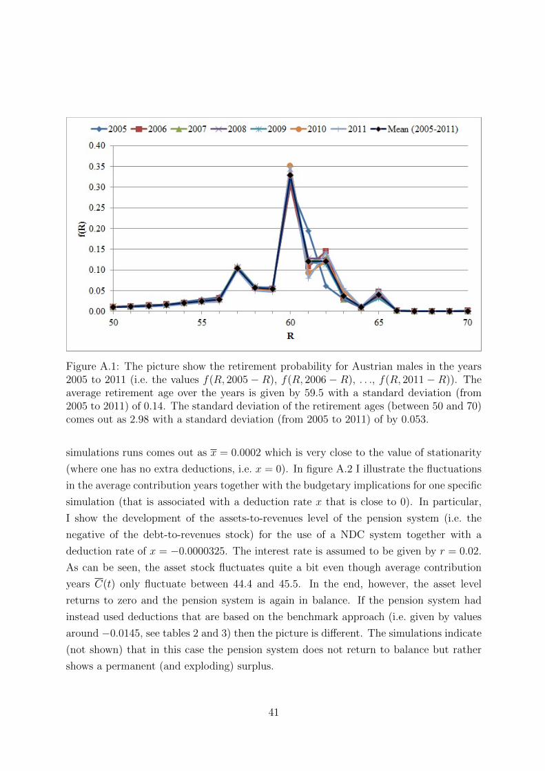
Figure A.1: The picture show the retirement probability for Austrian males in the years2005 to 2011 (i.e. the values f(R, 2005 − R), f(R, 2006 − R), . . ., f(R, 2011 − R)). Theaverage retirement age over the years is given by 59.5 with a standard deviation (from2005 to 2011) of 0.14. The standard deviation of the retirement ages (between 50 and 70)comes out as 2.98 with a standard deviation (from 2005 to 2011) of by 0.053.

simulations runs comes out as x = 0.0002 which is very close to the value of stationarity

(where one has no extra deductions, i.e. x = 0). In figure A.2 I illustrate the fluctuations

in the average contribution years together with the budgetary implications for one specific

simulation (that is associated with a deduction rate x that is close to 0). In particular,

I show the development of the assets-to-revenues level of the pension system (i.e. the

negative of the debt-to-revenues stock) for the use of a NDC system together with a

deduction rate of x = −0.0000325. The interest rate is assumed to be given by r = 0.02.

As can be seen, the asset stock fluctuates quite a bit even though average contribution

years C(t) only fluctuate between 44.4 and 45.5. In the end, however, the asset level

returns to zero and the pension system is again in balance. If the pension system had

instead used deductions that are based on the benchmark approach (i.e. given by values

around −0.0145, see tables 2 and 3) then the picture is different. The simulations indicate

(not shown) that in this case the pension system does not return to balance but rather

shows a permanent (and exploding) surplus.

41

(a) Average Contribution Years (b) Assets-Revenues-Ratio

Figure A.2: Panel (a) shows the fluctuations of the average contribution years for onespecific simulation where from some cohort onwards the contribution years are randomdraws from a triangular distribution. Panel (b) shows the implied fluctuations in theasset-to-revenues-ratio if pensions are based on a NDC system with a deduction rate ofx = −0.0000325 and the interest rate is given by r = 0.02.

C Stationary retirement in a model with growing

wages and non-rectangular mortality

This generalizes the model of section 3. The main results of the generalized model are

summarized in section 5.1 of the paper.

C.1 Set-up

C.1.1 Demographic structure

I work with a model in continuous time. In every instant of time t a new cohort is born.

The maximum age that a member of cohort t can reach is time-invariant and denoted by

ω. S(a) gives the probability that an individual survives to age a. It holds that S(0) = 1,

S(ω) = 0 and that survivorship declines with age, i.e. dS(a)da≤ 0 for a ∈ [0, ω]. The

mortality hazard rate is given by µ(a) ≡ −dS(a)da

1S(a)

. Therefore:

S(a) = e∫ a0 −µ(x) dx. (26)

An interesting benchmark case is given by rectangular survivorship where S(a) = 1 for

a ∈ [0, ω]. In this case there are no premature deaths and all members of a cohort reach

the maximum age ω. This corresponds to the assumption made in section 3.

42

Remaining life expectancy is given by:20

e(z) =

∫ ω

z

e∫ az −µ(x) dx da =

∫ ωzS(a) da

S(z). (27)

The second equality follows from the fact that e∫ az −µ(x) dx = e

∫ a0 −µ(x) dxe

∫ z0 µ(x) dx = S(a)

S(z)

where the last step uses equation (26).

The size of cohort t at age a is given by N(a, t) = N(0, t)S(a), where N(0, t) stands

for the initial size of the cohort. For the sake of simplicity I assume constant sizes of

birth cohorts, i.e. N(0, t) = N, ∀t. The entry age in the labor market is again assumed to

be constant and given by A while the age-specific probability to retire for generation t is

again given by f(a, t) for a ∈ [A, ω]. I assume that the mortality rates are independent

from this probability. The cumulative function F (a, t) then gives the percentage of the

surviving members of cohort t that are already retired at age a. It holds that F (A, t) = 0

and F (ω, t) = 1. In this appendix I focus on a stationary retirement distribution, i.e.

f(a, t) = f(a) and F (a, t) = F (a).

The total size of the active population L and the retired population M are constant

and given by:

L = N

∫ ω

A

S(a) (1− F (a)) da, (28)

M = N

∫ ω

A

S(a)F (a) da. (29)

C.1.2 Budget of the pension system

The contribution rate to the PAYG pension system is assumed to be fixed at τ . I abstract

from intragenerational wage differences and seniority profiles and simply assume that in

a specific period t each workers earns an identical wage W (t). Wages grow at rate g(t),

i.e. W (t) = W (0)e∫ t0 g(s) ds.

Each retired member of generation t receives a pension payment P (R, a, t). The size

of the pension can depend on the payment period t+a, on the individual’s age a and also

on the time of his or her retirement R ≤ a. Below I will say more about the determination

of the pension payments in different systems.

In order to calculate the total expenditures of the pension system one can make the

following considerations. First, focus on one particular retirement age R and calculate

the total of pension payments that is distributed to the group of pensioners that has

20See, e.g., Keyfitz & Caswell (2005) or Goldstein (2006).

43

retired at this age. This comprises individuals at different ages a ∈ [R,ω]. For a person

who is of age a in period t the pension payment is P (R, a, t − a) and the size of this

subgroup is N × S(a). The total payments to people with retirement age R in period

t is thus given by: P total(R, t) = N∫ ωRP (R, a, t − a)S(a) da. The same logic applies for

any possible retirement age R ∈ [A, ω] where the relative frequency of the retirement

age is given by f(R). Total pension expenditures in period t can thus be written as

E(t) =∫ ωAP total(R, t)f(R) dR or:21

E(t) = N

∫ ω

A

(∫ ω

R

P (R, a, t− a)S(a) da

)f(R) dR. (30)

Total revenues I(t), on the other hand, are given by:

I(t) = τW (t)L = τW (t)N

∫ ω

A

S(a) (1− F (a)) da. (31)

The total deficit (or surplus) of the pension system is given by D(t) = E(t)− I(t) while

the deficit ratio by d(t) = D(t)I(t)

= E(t)I(t)− 1. A continuously balanced budget is thus

characterized by D(t) = d(t) = 0,∀t.

C.2 Different PAYG systems

In the last section C.5 of this appendix I discuss in detail how the pension level Pj(R, a, t)

is determined in the three different pension systems j ∈ {DB,AR,NDC}. Here I only

summarize the main results. There are two main differences to the simple model of

sections 2 and 3 that have to do with the assumptions of growth and mortality. All

pension systems have to specify how pension claims that have been acquired in the past

are revalued at the moment of retirement. In the NDC system, e.g., this is done by the

choice of a “notional interest rate” ρ(a, t). There exist two popular variants of this interest

rate that are discussed in the literature and used in real-world systems:

ρ(a, t) = g(t) + µ(a) (32a)

or

ρ(a, t) = g(t). (32b)

21Alternatively, one could also reverse the order and look first at a fixed age a of the retired populationand calculate the total pension payments to those individuals that have different retirement ages R. In thesecond step one would then calculate the total pension payments to all possible ages a. This results in anequivalent expression. I focus on the formulation in (30) since it is more convenient for later calculations.

44

Both notional interest rates reflect the growth rate of average wages g(t) while the first

specification (32a) also corrects for the fact that each period some cohort members die.

The account values of the deceased cohort members are regarded as “inheritance gains”

that are distributed among surviving cohort members by granting an extra return µ(a).

For later reference it is also useful to define the following term:

h(R) ≡∫ RAS(a) da

(R− A)S(R), (33)

that stands for the “per capita inheritance gains premium”, i.e. the factor by which the

first pension at retirement age R is higher if the revaluation takes inheritance gains into

account. For rectangular survivorship there are no inheritance gains and thus the average

premium is h(R) = 1.

Furthermore, due to the assumption of a growing economy one also has to specify how

pension are adjusted over time. Here it is assumed (for simplicity and in line with the

practice in many countries) that ongoing pensions are adjusted with the average growth

rate of wages, i.e.%

ϑ(t) = g(t). (34)

In section 5.3 of the paper I also discuss briefly the consequences of the assumption

ϑ(t) = 0.

In section C.5 I show that in this situation the three pension system are associated

with the following pension levels:

PNDC(R, a, t) = τW (t+ a)(R− A)h(R)

e(R)XNDC(R, t), (35)

PDB(R, a, t) = q∗W (t+ a)XDB(R, t), (36)

PAR(R, a, t) = κ∗W (t+ a)(R− A)XAR(R, t), (37)

where the NDC system uses the notional interest including inheritance gains (i.e. equation

(32a)) to revalue past contributions. This is in line with the approach used in Sweden.

The other two system are based on indexations excluding these mortality adjustments (i.e.

on equation (32b)) which is also in line with the real-world systems. All three pension

system also allow for the use of demographic adjustment factors Xj(R, t) as discussed in

section 2. In the case of non-stationary constellations the deduction factor might also be

time-dependent as is indicated by the use of a time index t.

45

C.3 Budget-neutral deductions

In this part I investigate how the deduction factors Xj(R, t) have to be determined in

order to guarantee a balanced PAYG system in the case of a stationary demographic

situation. The following proposition is a generalization of proposition 1. It states that a

standard NDC system with ρ(a, t) = g(t) + µ(a) leads to a balanced budget without the

need for further deductions.

Proposition 2

Assume a stationary demographic situation where the size of birth cohorts is constant

(N(0, t) = N), people start to work at age A, the maximum age is ω, mortality is described

by the survivorship function S(a) for a ∈ [0, ω], retirement age is distributed according

to the density function f(R) for R ∈ [A, ω] and wages grow with rate g(t). In this case

a NDC system will be in continuous balance (E(t) = I(t),∀t) if the notional interest

rate and the adjustment factor are set according to ρ(a, t) = g(t) + µ(a) (equation (32a))

and ϑ(t) = g(t) (equation (34)), respectively, and if there are no additional deductions

(XNDC(R, t) = 1).

Proof. For the NDC system one can insert the pension level from equation (35), i.e.

PNDC(R, a, t− a) = τW (t) (R−A)h(R)e(R)

XNDC(R, t) into (30) to conclude that:

E(t) = τW (t)N

∫ ω

A

(R− A)h(R)

e(R)XNDC(R, t)

(∫ ω

R

S(a) da

)f(R) dR

= τW (t)N

∫ ω

A

(∫ R

A

S(a) da

)XNDC(R, t)f(R) dR, (38)

where I use the definitions h(R) =∫RA S(a) da

(R−A)S(R)and e(R) =

∫ ωRS(a) da

S(R).

For the assumptions of proposition 2 total expenditures in equation (38) can be written

as:

E(t) = τW (t)N

∫ ω

A

(∫ R

A

S(a) da

)f(R) dR.

One can define u(R) =∫ RAS(a) da and v(R) = 1− F (R) with u′(R) = S(R) and v′(R) =

−f(R). Using integration by parts it holds that:∫ ω

A

(∫ R

A

S(a) da

)f(R) dR = −

∫ ω

A

u(R)v′(R) dR = −u(R)v(R) +

∫ ω

A

u′(R)v(R) dR.

46

The term (−u(R)v(R)) is given by[(∫ R

AS(a) da

)(1− F (R))

]ωA

which can be evaluated

as (∫ ω

A

S(a) da

)(1− F (ω))−

(∫ A

A

S(a) da

)(1− F (A)) = 0. (39)

Since it holds that∫ ωAu(R)v′(R) dR =

∫ ωAS(R)(1− F (R)) dR one can conclude that:

E(t) = τW (t)N

∫ ω

A

S(R)(1− F (R)) dR. (40)

This is equal to total revenues I(t) = τW (t)N∫ ωAS(a) (1− F (a)) da (see (31)) and thus

E(t) = I(t).

Proposition 2 generalizes proposition 1 and it confirms the previous findings. For a

stationary economic and demographic situation a NDC system that includes a correction

for inheritance gains is stable if one uses the benchmark NDC formula:

PNDC(R, a, t) = τW (t+ a)(R− A)h(R)

e(R). (41)

There is no need for an additional adjustment factor and it holds (as in section 3.2) that

XNDC(R, t) = ΨNDC(R) = 1.

In this case it is also possible to make the DB and the AR systems stable by just using

demographic deduction factors ΨDB(R) and ΨAR(R) that are independent of the discount

rate δ and of time t. These are calculated in appendix C.5.22 As in section 2 I again invoke

the “balanced target condition”, i.e. the condition that the target replacement rate q∗ is

chosen in such a way that if everybody retires at the target retirement age R∗ there will

be no deductions (ΨDB(R∗) = 1) and the system will be in balance (see section 5.3 for

a discussion of the situation without a balanced budget). The demographic adjustment

factors come out as:

ΨDB(R) =e(R∗)

e(R)

h(R)

h(R∗)

R− AR∗ − A

, (42)

ΨAR(R) =e(R∗)

e(R)

h(R)

h(R∗). (43)

In table A.1 I collect important formulas for the three PAYG systems. In particular, it

contains the formula pension Pj(R, a, t) (both in its basic form and after invoking the

22I also discuss the case of a NDC system that uses (32b) instead of (32a), i.e. that excludes thecorrection for inheritance gains in the notional interest rate. In this case one also needs a demographicadjustment factor in order to implement a balanced system.

47

Table A.1: Three PAYG systems for a stationary demography

(1) (2) (3) (4)

Type Pj(R, a, t) Pj(R, a, t) Ψj Pj(R, a, t)(j) (for BTC) (for BTC)

DB q∗W (t+ a) τW (t+ a) (R∗−A)h(R∗)e(R∗)

e(R∗)

e(R)h(R)

h(R∗)R−AR∗−A τW (t+ a) (R−A)h(R)

e(R)

AR κ∗(R− A)W (t+ a) τW (t+ a) (R−A)h(R∗)

e(R∗)

e(R∗)

e(R)h(R)

h(R∗)

τW (t+ a) (R−A)h(R)e(R)

NDC τW (t+ a) (R−A)h(R)e(R)

τW (t+ a) (R−A)h(R)e(R)

1 τW (t+ a) (R−A)h(R)e(R)

Note: The table shows the formula pension Pj(R, a, t), the demographic deduction factor Ψj and the

total pension Pj(R, a, t) = Pj(R, a, t)Ψj for three variants of PAYG schemes: DB (Defined Benefit), AR(Accrual Rates), NDC (Notional Defined Contribution). The balanced target condition (BTC) has to holdif the system has a balanced budget in the case that all individuals retire at the target retirement ageR = R∗. These are specified in the text. Column (4) is the multiple of columns (2) and (3).

balanced target condition), the demographic deduction factor Ψj and the final pension

Pj(R, a, t) = Pj(R, a, t)Ψj. Note that for rectangular survivorship it holds that h(R) = 1

and e(R) = ω − R . In this case the results of table A.1 coincide with the ones of table

1. In particular, ΨDB(R) = ω−R∗ω−R

R−AR∗−A and ΨAR(R) = ω−R∗

ω−R .

C.4 The choice of discount rates

So far I have shown that for a stationary economic and demographic situation a standard

NDC system implements a stable PAYG pension system. By using the correct demo-

graphic adjustment factors ΨDB and ΨAR also the DB and a AR systems can be amended

to guarantee a continuous budgetary balance. This implies that it is not necessary to

refer to the market interest rate in order to design the budget-neutral deduction rates in

this stationary constellation.

It is interesting to look at this issue from the viewpoint of the standard deduction

framework presented in section 2.2 and ask a number of questions. First, which choice of

the discount rate will give rise to the budget-neutral demographic deduction factors Ψj?

Second, what deductions are implied if the discount rate is set to higher levels? Third,

under which conditions will higher discount rates also be compatible with a balanced

budget? Answers to these questions will be provided in the next three subsections.

48

C.4.1 The appropriate budget-neutral discount rate for a stationary demog-

raphy

In order to find the discount rate that is compatible with the budget-neutral demographic

deduction factors Ψj one has to adapt the neutrality condition (1) of section 2.2 for the

general framework. It comes out as:

∫ R∗R

(τW (t+ a) + Pj(R, a, t)Xj

)e−δ(a−R)S(a) da =∫ ω

R∗

(Pj(R

∗, a, t)− Pj(R, a, t)Xj

)e−δ(a−R)S(a) da. (44)

I want to know for which choice of δ the total deduction factor will collapse to the

demographic factor, i.e. for which δ it holds that Xj = Ψj. In general, one cannot solve

(44) for Xj in closed form. In the following I show, however, analytically that for the case

of constant growth (i.e. g(t) = g) the choice of δ = g leads to the result that Xj = Ψj.

In order to do so I focus on formula pensions that are proportional to τW (t + a).

Therefore I write P (R, a, t) = τW (t + a)P (R). Furthermore, noting that W (t + a) =

W (t+R)e∫ aRg(t+s) ds equation (44) can also be written as:

τW (t+R)

∫ R∗

R

(1 + P (R)X

)e∫ aRg(t+s) dse−δ(a−R)S(a) da =

τW (t+R)

∫ ω

R∗

(P (R∗)− P (R)X

)e∫ aRg(t+s) dse−δ(a−R)S(a) da.

For constant wage growth g(s) = g this can be simplified to:23

∫ R∗R

(1 + P (R)X

)e−(δ−g)(a−R)S(a) da =∫ ω

R∗(P (R∗)− P (R)X

)e−(δ−g)(a−R)S(a) da. (45)

I want to show that for the choice of δ = g the deductionsX coincide with the demographic

deduction factor Ψ. I focus first on the NDC system. In this case it holds that Ψ = 1

and the conjecture is that X = Ψ = 1. Furthermore, P (R, a, t) = τW (t + a) (R−A)h(R)e(R)

,

i.e. P (R) = (R−A)h(R)e(R)

. Noting that h(R) =∫RA S(a) da

(R−A)S(R)and e(R) =

∫ ωRS(a) da

S(R)one can thus

23Similarly, one could also assume a time-varying discount rate δ(s). Under the assumption thatδ(s) = g(s) one could then derive the same result as in the following.

49

write: P (R) =∫RA S(a) da∫ ωRS(a) da

. Inserting this into (45) leads to:

(1 +

∫ RAS(a) da∫ ω

RS(a) da

)∫ R∗

R

S(a) da =

(∫ R∗AS(a) da∫ ω

R∗S(a) da

−∫ RAS(a) da∫ ω

RS(a) da

)∫ ω

R∗S(a) da.

This can be simplified to:(∫ ωRS(a) da+

∫ RAS(a) da

) ∫ R∗RS(a) da =(∫ R∗

AS(a) da

∫ ωRS(a) da−

∫ RAS(a) da

∫ ωR∗S(a) da

).

Collecting terms this leads to:

∫ ω

R

S(a) da

(∫ R∗

R

S(a) da−∫ R

∗

A

S(a) da

)=

∫ R

A

S(a) da

(−∫ ω

R∗S(a) da−

∫ R∗

R

S(a) da

).

Combining integrals one can conclude:

−(∫ ω

R

S(a) da

∫ R

A

S(a) da

)= −

(∫ ω

R

S(a) da

∫ R

A

S(a) da

).

This proves the conjecture that for δ = g the implied deduction X equals the demographic

deduction Ψ which is just Ψ = 1 for the NDC system. Since the demographic deduction

factors ΨDB and ΨAR are just determined in such a way as to transform the DB and AR

systems into a NDC system the same conclusion also holds for these systems.

The stated result implies that the appropriate budget-neutral discount rate for a sta-

tionary situation is given by the internal rate of return. This has often been claimed in

the related literature but the present framework allows to formulate it in a precise manner

and to state the exact conditions (in particular demographic stationarity) under which it

holds.

C.4.2 Deductions for different discount rates

In a next step one can investigate which deductions are implied by choices of the discount

rate δ > g. Although these choices are not necessary from the viewpoint of budgetary

stability it is nevertheless instructive to see the magnitudes involved. To do so I use

illustrative numerical examples. In particular, I assume a Gompertz survival curve of the

50

Table A.2: Deductions for R = 64 and R∗ = 65

δ = 0 δ = 0.02 δ = 0.05

Type j Pj Ψj Xj xj(in%) Pj Xj xj(in%) Pj Xj xj(in%) PjDB 67.0 0.93 0.93 -7.04 62.3 0.91 -8.71 61.1 0.89 -11.49 59.3AR 65.5 0.95 0.95 -4.92 62.3 0.93 -6.64 61.1 0.91 -9.48 59.3NDC 62.3 1 1 0 62.3 0.98 -1.81 61.1 0.95 -4.79 59.3

Note: The table shows the actuarial deduction factors Xj , the annual deductions rates xj (based on the

linear relation xj =Xj−1

R∗−R ) and the final pension Pj(R,R

∗) = Pj(R,R∗)Xj for three pension schemes and

three (net) discount rates δ ≡ δ − g. For the sake of comparison also the values of the pure demographicdeduction factors Ψj are reported. The numerical values are: A = 20, τ = 0.25, g = 0.02, R∗ = 65 andR = 64. For all three schemes the target pension is P ∗ = 67. Mortality follows a Gompertz distributionwith α = 0.000025 and β = 0.096.

form S(a) = eαβ (1−eβa).24

In Tables A.2 and A.3 I report the deduction factors Xj and annual deduction rates xj

for various assumption concerning the (net) discount rate δ ≡ δ − g. They correspond to

tables 2 and 3 from section 2.2 which were based on rectangular survivorship. In addition, I

also report the demographic deduction factors Ψj that are sufficient for budgetary stability.

For all three systems the target pension level at the target retirement age R∗ = 65 is given

by P ∗ = 67 (which implies a target replacement rate for the DB system of q∗ = 0.67). This

is lower than for the case of rectangular survivorship since —due to premature deaths—

remaining life expectancy e(R∗) at R∗ = 65 is now larger (18.6 vs. 15). The step-up

of pensions due to inheritance gains is non-trivial and given by h(R∗) = 1.11 (or 11%).

This is due to the fact that only 88% of all members of a cohort survive up to this age

(S(R∗) = 0.88).

The results are qualitatively similar to the ones for rectangular survivorship in tables 2

and 3. The first thing to note is that for δ = 0 (i.e. δ = g) the total deductions correspond

exactly to the demographic adjustment factors, i.e. Xj = Ψj as has already been shown

in section C.4.1. For the DB system the correct annual deduction rate for a retirement

at the age of 64 is 7% while it is 4.9% for the AR system if mortality follows a Gompertz

24The associated mortality rate is given by µ(a) = αeβa (i.e. the logarithm of mortality rates increaseslinearly in age). The Gompertz-function delivers a good description of empirical mortality data. For thefollowing examples I use a parameterization of α = 0.000025 and β = 0.096. This is roughly based onthe Austrian life tables from 2005 which have the convenient property that the (unisex) life expectancyat birth was almost exactly 80 which facilitates comparisons to the numerical examples of section 2 withrectangular survivorship.

51

Table A.3: Deductions for R = 60 and R∗ = 65

δ = 0 δ = 0.02 δ = 0.05

Type j Pj Ψj Xj xj(in%) Pj Xj xj(in%) Pj Xj xj(in%) PjDB 67.0 0.7 0.7 -5.94 47.1 0.64 -7.28 42.6 0.53 -9.36 35.6AR 59.5 0.79 0.79 -4.18 47.1 0.72 -5.69 42.6 0.6 -8.04 35.6NDC 47.1 1 1 0 47.1 0.9 -1.91 42.6 0.76 -4.87 35.6

Note: See table A.2 with the difference that now R = 60 instead of R = 64.

pattern. This is smaller than the corresponding rates for rectangular survival where they

have been calculated as 8.33% and 6.25%, respectively. For larger discount rates, however,

the difference shrinks and for δ = 0.05, e.g., the annual deduction rates for the Gompertz

and the rectangular case are very similar (11.49%, 9.48% and 4.79% vs. 11.81%, 9.8% and

3.79%). A parallel conclusion holds for the case of R = 60 where the differences between

the results of table A.3 (Gompertz) and table 3 (rectangular) are even smaller.

C.4.3 Balanced and unbalanced budgets for different discount rates

In the simple framework of sections 2 and 3 I have shown that even for discount rates

that are larger than necessary it might still be the case that the system runs a balanced

budget. In particular, I have shown in section 4 that the balanced budget condition

depends on the choice of both the discount rate δ and the target retirement age R∗.

This can be repeated for the general framework. It is not possible to derive closed-form

solutions for the balanced budget and one has to resort to numerical calculations. In

particular, I assume that retirement ages follow a triangular distribution that is defined

by the minimum and maximum retirement ages RL and RH , respectively and also by

the mode Rmod. The density function is then given by f(R) = 2(R−RL)(RH−RL)(Rmod−RL)

for

RL ≤ R ≤ Rmod and f(R) = 2(RH−R)

(RH−RL)(RH−Rmod)

for Rmod ≤ R ≤ RH .25

In table A.4 I show three distributions that differ in the shape and the average retire-

ment age R = RL+R

mod+R

H

3. In all three distributions I assume that the earliest retirement

age is given by RL = 60. In the first distribution RH = 70 and the modus, median and

mean coincide at Rmod = R = 65. In the second distribution the modus is again Rmod = 65

while the maximum retirement age is RH = 67 implying a mean of R = 64. Finally, for

25I have also analyzed different retirement distributions. The results are robust.

52

Table A.4: Deficit ratios d = E/I

Distribution 1 Distribution 2 Distribution 3

Type j δ = 0 δ = 0.02 δ = 0.05 δ = 0 δ = 0.02 δ = 0.05 δ = 0 δ = 0.02 δ = 0.05

DB 1 1 1.004 1 0.982 0.954 1 1.001 1.003AR 1 1 1.004 1 0.982 0.954 1 1 1.003NDC 1 1 1.004 1 0.982 0.954 1 1 1.003

Note: The table shows the deficit ratio for three pension schemes, three assumptions of the discount rate δ ≡ δ−gand three assumed distributions of the retirement age. These are RL = 60, Rmod = 65, RH = 70 (distribution

1), RL = 60, Rmod = 65, RH = 67 (distribution 2) and RL = 60, Rmod = 67, RH = 68 (distribution 3). Themean retirement age is R = 65 for distributions 1 and 3 and R = 64 for distribution 2. Mortality follows aGompertz distribution with α = 0.000025 and β = 0.096 and the target retirement age is always R∗ = 65.

the third distribution I assume a non-symmetric case with R = 68 and Rmod = 67 which

implies an average retirement age of R = 65.

The first result is that the budget is in balance for all three distributions of retirement

ages as long as the discount rate is equal to the growth rate of wages (i.e. δ = 0). This is

of course an expected result that follows from the analytical findings of section C.4.1. As

a second result one can see that the budget is also (approximately) balanced for situations

where δ > 0 as long as R∗ = R (which is the case for distributions 1 and 3). For the

second distribution, however, for which R∗ = 65 > 64 = R this is different. In this case

the pension system runs a permanent surplus if the discount rate is above the growth rate

of wages (d = 0.98 for δ = 0.02 and d = 0.95 for δ = 0.05).

These results are completely parallel to the ones of section 3. In particular, the budget

is balanced as long as the discount rate is set equal to the growth rate of wages (as has

already been shown analytically in section C.4.1). Furthermore, the budget also turns out

to be (approximately) balanced for situations where the discount rate differs from this

benchmark value as long as R∗ = R.

C.5 Derivation of the pension formulas for the different systems

In this section I derive the formulas for the diferent pension systems that have been stated

and used above in section C.2.

53

C.5.1 Notional defined contribution pension system

I start with the discussion of how the pension level P (R, a, t) is determined in NDC

systems. This provides again a useful benchmark case to derive the necessary deductions

and supplements for the two other PAYG pension systems (AR and DB).

The contributions in a NDC system are credited to a notional account and they are

revalued with a “notional interest rate” ρ(a, t) (that is allowed to change over time and

across ages). The total value of this account is called the “notional capital” that accumu-

lates over the working periods of an insured person. When the individual retires at age

R the final notional capital is given by:

K(R, t) =

∫ R

A

τW (t+ x)e∫Rx ρ(s,t+s) ds dx, (46)

where the cumulative factor e∫Rx ρ(s,t+s) ds indicates how the contribution τW (t + x) that

is paid into the pension system in period t + x is revalued when calculating the final

amount of the notional capital in period t + R (the period of retirement). The notional

interest rate is a crucial magnitude in a NDC system as I discuss in a different paper (see

Knell 2017a). In section C.2 I use two standard definitions that can be found in real-world

NDC systems. Both notional interest rates are related to the growth rate of productivity

(or of average wages) while one also contains a correction for the fast that the cohort

size decreases with the mortality rate µ(a). The account values of the deceased cohort

members are regarded as “inheritance gains” that are distributed among surviving cohort

members by granting an extra return µ(a). In particular:

ρ(a, t) = g(t) + µ(a)

or

ρ(a, t) = g(t),

which corresponds to equations (32a) and (32b) in section C.2. Using these definitions

for the notional interest rate in (46) one can conclude that K(R, t) = τW (t+R)(R−A)

if one uses the value of ρ(a, t) without inheritance gains (equation (32b)) or K(R, t) =

τW (t+R)∫ RAe∫Ra µ(s) ds da if one uses the specification that includes the inheritance gains

(equation (32a)). This can also be written as K(R, t) = τW (t + R)(R − A)h(R), where

h(R) ≡∫RA S(a) da

(R−A)S(R)as expressed in equation (33). The term h(R) stands for the per capita

“inheritance gains premium” to the “normal” notional capital, averaged over the (R−A)

54

contribution periods and distributed among the mass S(R) of surviving members.26

The first pension that is received by a member of cohort t who retires at the age R is

given by:

PNDC(R,R, t) =K(R, t)

e(R)XNDC(R, t). (48)

The first pension is calculated by taking the final notional capital K(R, t) and turning it

into an annual pension payment by using remaining life expectancy e(R) as the annuity

conversion factor. In addition, there might also be a deduction factor XNDC(R, t) that

is applied to secure a balanced budget if the formula pension K(R,t)e(R)

is not sufficient.

For simplicity I write this demographic deduction factor only as a function of the actual

retirement age R and time although—in general—it will also depend on other demographic

and policy variables (like R∗ and A). The dependence on time is relevant for the case of

non-stationary retirement distributions.

From equation (27) it is known that:

e(R) =

∫ ωRS(a) da

S(R). (49)

This can be used together with K(R, t) = τW (t+ R)(R− A)h(R) = τW (t+ R)∫RA S(a) da

S(R)

to derive the first pension in the case that the notional interest rate includes a correction

for the inheritance gains (i.e. ρ(a, t) = g(t) + µ(a)):

PNDC(R,R, t) = τW (t+R)(R− A)h(R)

e(R)XNDC(R, t)

= τW (t+R)

∫ RAS(a) da∫ ω

RS(a) da

XNDC(R, t). (50)

This expression is quite intuitive. At the moment of retirement the first pension payment

is proportional to the wage level in the period of retirement t+R. This is due to the fact

that past contributions are indexed to average wage growth. The inclusion of inheritance

gains raises the notional capital (which is captured by the expression in the numerator)

while the period pension payment depends on remaining life expectancy (which is captured

by the expression in the denominator). In addition there might be a correction for early

or late retirement XNDC(R, t).

26The relation follows by noting that e∫ R

aµ(s) ds can be written as: e

∫ R

aµ(s) ds = e

∫ R

0µ(s) dse

∫ a

0−µ(s) ds.

Therefore∫ RAe∫ R

aµ(s) ds da = e

∫ R

0µ(s) ds ∫ R

Ae∫ a

0−µ(s) ds da = (S(R))

−1 ∫ RAS(a) da, where I use (26).

55

For the situation where inheritance gains are not included and where the notional

interest rate is simply given by ρ(t) = g(t) the first pension is:

PNDC′(R,R, t) = τW (t+R)R− Ae(R)

XNDC′(R, t)

= τW (t+R)R− A∫ ωRS(a) da

S(R)

XNDC′(R, t). (51)

For the case of rectangular survivorship (S(a) = 1 for a ∈ [A, ω]) one gets that both (50)

and (51) lead to the same result that PNDC(R,R, t) = τW (t+R)R−Aω−RXNDC(R, t). This is

the same expression that was used in section 2 (see table 1).

Existing pensions are adjusted according to:

Pj(R, a, t) = Pj(R,R, t)e∫ aRϑ(t+s) ds, (52)

for a ∈ [R,ωc(t)] and where I use the index j since the adjustment in (52) is valid for all

three pension systems j ∈ {DB,AR,NDC}. The variable ϑ(t) stands for the adjustment

rate in period t and the cumulative adjustment factor e∫ aRϑ(t+s) ds indicates how the first

pension P (R,R, t) is adjusted to give the pension payment in period t+ a. In section C.2

I assume that ongoing pensions are adjusted with the average growth rate of wages as

expressed in equation (34) stating that ϑ(t) = g(t).

In this case one can use (50) and (52) to conclude that with ρ(a, t) = g(t) + µ(a) the

ongoing pension is:

PNDC(R, a, t) = τW (t+ a)(R− A)h(R)

e(R)XNDC(R, t),

which is equation (35) in section C.2. For ρ(a, t) = g(t) it holds that PNDC′(R, a, t) =

τW (t + a)R−Ae(R)

ΨNDC′(R). In the following I focus on the first case with a compensation

for inheritance gains.

C.5.2 Defined benefit pension system

In a similar vein one can look at the two alternative pension systems discussed in section

2. The defined benefit (DB) system promises a target replacement rate q∗ if an individual

retires at the target retirement age R∗. The replacement rate is related to average lifetime

income, where past incomes are revalued at a rate ρ(a, t) and where there are correction

56

for early/late retirement. In particular, instead of (48) it now holds that:

PDB(R,R, t) = q∗WLT

(R, t)XDB(R, t), (53)

whereWLT

(R, t) =∫RAW (t+x)e

∫Rx ρ(s,t+s) ds dx

R−A . This expression is closely related to the notional

capital (46) for NDC systems. I know of no existing DB system that includes a correction

for inheritance gains when indexing past wage levels. Therefore the benchmark DB system

is characterized by the indexation ρ(a, t) = g(t). From this is follows that PDB(R,R, t) =

q∗W (t + R)XDB(R, t). As above I assume that existing pension are adjusted with the

growth rate of average wages according to (52) and (34) and thus:

PDB(R, a, t) = q∗W (t+ a)XDB(R, t),

which corresponds to equation (36) in section C.2.

C.5.3 Accrual rate pension system

Finally, one can look at the accrual rate system in the general set-up. The AR system

promises a pension that is proportional to the revalued average lifetime income. In par-

ticular, for each year of work the system promises a certain percentage κ∗ (the accrual

rate) of this lifetime average that can be claimed at the target retirement age R∗. For

early retirement there exists a deduction XAR(R, t). In particular, the first pension is now

defined as:

PAR(R,R, t) = κ∗(R− A)WLT

(R, t)XAR(R, t), (54)

where WLT

(R, t) stands for lifetime income (as defined in section C.5.2) for which past

incomes are revalued at a rate ρ(a, t). As before and in line with existing AR system I

assume that indexation follows the growth rate of average wages, i.e. ρ(a, t) = g(t). From

this is follows that PAR(R,R, t) = κ∗W (t+R)(R−A)XAR(R, t). For pension adjustment

according to (52) and ϑ(t) = g(t) one can conclude that:

PAR(R, a, t) = κ∗W (t+ a)(R− A)XAR(R, t).

which corresponds to equation (37) in section C.2.

57

C.5.4 Demographic adjustment factors

Proposition 2 shows that for a stationary retirement distribution f(R) the NDC system

is stable for X(R, t) = Ψ(R) = 1. It is now straightforward to discuss the demographic

deductions Ψj(R) that are necessary to establish balanced budget for pension systems that

deviate from the NDC benchmark. This can be seen by looking at equation (38). If the

pension payments of the alternative system can be written as Pj(R, a, t) = τW (t+a) (· · · )then the correction Ψj(R) just has to be set in a way such that it mimics the benchmark

NDC-pension given in (41). As a first example one can look at a NDC ′ system that

does not include the compensation for inheritance gains (as is the case for most existing

NDC systems with the notable exception of Sweden) and that sets ρ(a, t) = g(t). In

this case it has been shown above that the pension is given by PNDC′(R, a, t) = τW (t +

a) (R−A)e(R)

ΨNDC′(R). It is immediately apparent that an adjustment with ΨNDC

′(R) = h(R)

leads to a balanced budget. Otherwise, the pension system would run a surplus since

h(R) > 1, i.e. the system would keep the inheritance gains for itself instead of distributing

them among the surviving population.

For the defined benefit system I invoke as in section 2 the “balanced target con-

dition”, i.e. I assume that the target replacement rate q∗ is associated with a situa-

tion that there will not be any deductions (ΨDB(R∗) = 1) if everybody retires at the

target retirement age R∗. For the NDC system one knows from equation (41) that

a balanced budget with R = R∗,∀i requires that everybody gets a pension equal to

PNDC(R∗, a, t) = τW (t + a) (R∗−A)h(R∗)e(R∗)

. This should be equal to the DB pension with

R = R∗,∀i, i.e. to PDB(R∗, a, t) = q∗W (t + a). From these two expressions it follows

that q∗ = τ (R∗−A)h(R∗)e(R∗)

. Inserting this into equation (36) for PDB(R, a, t) leads to the DB

pension after evoking the stability condition:

PDB(R, a, t) = τW (t+ a)(R∗ − A)h(R∗)

e(R∗)ΨDB(R). (55)

This expression can now be compared to the pension of the benchmark NDC system (41)

(that leads to a balanced budget) to conclude that ΨDB(R) = R−AR∗−A

e(R∗)

e(R)h(R)

h(R∗)

as stated in

equation (42).

One can use similar steps for the AR pension system. In particular, I assume that the

target accrual rate κ∗ is chosen in such a way that the system is balanced if everybody

retires at the target retirement age R = R∗,∀i. Inserting the implied target accrual rate

κ∗ = τ h(R∗)

e(R∗)

into equation (37) for PAR(R, a, t) leads to the AR pension after evoking the

58

stability condition:

PAR(R, a, t) = τW (t+ a)(R− A)h(R∗)

e(R∗)ΨAR(R). (56)

The deduction rate that is necessary for a balanced AR system can be calculated by setting

(56) equal to the NDC pension (41) and solving for ΨAR(R). This leads to ΨAR(R) =e(R∗)

e(R)h(R)

h(R∗)

as stated in equation (43). These and other important formulas are collected

in table A.1 of section C.2.

D Extensions (section 5)

In the main part of the paper I have assumed that all individuals have the same entry

age A, the same wage level W and the same life expectancy ω. In this part of the paper

I broaden up this framework and now assume that the society is split in j = 1, 2, . . . J

groups (with respective weight πj) where each group is characterized by specific values

for Aj, Wj, ωj and possibly also R∗j (i.e. the system might prescribe group-specific target

retirement ages).27 A possible correlation between income, entry age, life expectancy

etc. is captured by the pattern of relative frequencies πj of the different groups with∑Jj=1 πj = 1. Although members of each group are identical along all the above mentioned

dimensions they might differ in their retirement age. In particular, I assume that within

each group j there are k = 1, 2, . . . K subgroups of individuals with a retirement age

Rkj and a relative frequency φkj with

∑Kk=1 φ

kj = 1. The within-group differences in the

retirement age are important in order to calculate the appropriate deductions for early

retirement at the age of Rkj instead of R∗j .

Throughout the following analyses I assume that the formula of the NDC system is

based on average life expectancy ω =∑J

j=1 πjωj = 1 rather than on group-specific life

expectancy ωj. This might be due to reasons of information availability or political choice.

It will become apparent that this fact has major budgetary and distributional implications

while heterogeneity in the other variables does not affect the main conclusions.

27In fact, one could also introduce heterogeneous wage profiles. Assume that group j of the cohort bornin period t earned a wage Wj(a, t) = ξj(a, t)W (t + a) in each of its working period between age Aj andage Rj where W (t) now is the aggregate wage in period t. For the NDC system the notional capital would

then be given by Kj(Rj , t) = τW (t + R)(Rj − Aj)EP j , where EP j ≡(∫ Rj

Ajξj(a, t+ a) da

)/(Rj − Aj)

stands for the average lifetime “earnings points” (to use an expression from the German pension system).If group j had always earned average wages then ξj(a, t+ a) = 1,∀a and EP j = 1.

59

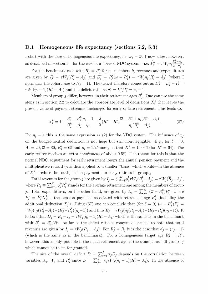
D.1 Homogeneous life expectancy (sections 5.2, 5.3)

I start with the case of homogeneous life expectancy, i.e. ωj = ω. I now allow, however,

as described in section 5.3 for the case of a “biased NDC system”, i.e. P kj = τWjηj

Rkj−Ajω−Rkj

.

For the benchmark case with Rkj = R∗j for all members k, revenues and expenditures

are given by I∗j = τWj(R∗j − Aj) and E∗j = P ∗j (ω − R∗j ) = τWjηj(R

∗j − Aj) (where I

normalize the cohort size to Nj = 1). The deficit therefore comes out as D∗j = E∗j − I∗j =

τWj(ηj − 1)(R∗j − Aj) and the deficit ratio as d∗j = E∗j /I∗j = ηj − 1.

Members of group j differ, however, in their retirement ages Rkj . One can use the same

steps as in section 2.2 to calculate the appropriate level of deductions Xkj that leaves the

present value of payment streams unchanged for early or late retirement. This leads to:

Xkj = 1 +

R∗j −Rkj

Rkj − Aj

ηj − 1

ηj− δ

2(R∗ −Rk

j )ω −R∗j + ηj(R

∗j − Aj)

ηj(Rkj − Aj)

. (57)

For ηj = 1 this is the same expression as (2) for the NDC system. The influence of ηj

on the budget-neutral deduction is not huge but still non-negligible. E.g., for δ = 0,

Aj = 20, ω = 80, R∗j = 65 and ηj = 1.25 one gets that Xkj = 1.0046 (for Rk

j = 64). The

early retiree receives an extra supplement of about 0.5%. The reason for this is that the

normal NDC adjustment for early retirement lowers the annual pension payment and the

multiplicative reward ηj is thus applied to a smaller “base” which would—in the absence

of Xkj —reduce the total pension payments for early retirees in group j.

Total revenues for the group j are given by Ij =∑K

k=1φkj τWj(R

kj−Aj) = τWj(Rj−Aj),

where Rj ≡∑K

k=1 φkjR

kj stands for the average retirement age among the members of group

j. Total expenditures, on the other hand, are given by Ej =∑K

k=1(ω − Rkj )P

kj , where

P kj = P k

j Xkj is the pension payment associated with retirement age Rk

j (including the

additional deduction Xkj ). Using (57) one can conclude that (for δ = 0) (ω − Rk

j )Pkj =

τWj(ηj(Rkj−Aj)+(R∗j−Rk

j )(ηj−1)) and thus Ej = τWj(ηj(Rj−Aj)+(R∗j−Rj)(ηj−1)). It

follows that Dj = Ej − Ij = τWj(ηj − 1)(R∗j −Aj) which is the same as in the benchmark

with Rkj = R∗j ,∀k. As far as the deficit ratio is concerned one has to note that total

revenues are given by Ij = τWj(Rj − Aj). For R∗j = Rj it is the case that dj = (ηj − 1)

(which is the same as in the benchmark). For a homogeneous target age R∗j = R∗,

however, this is only possible if the mean retirement age is the same across all groups j

which cannot be taken for granted.

The size of the overall deficit D =∑J

j=1 πjDj depends on the correlation between

variables Aj, Wj and R∗j since D =∑J

j=1 πjτWj(ηj − 1)(R∗j − Aj). In the absence of

60

a ‘bias” (i.e for ηj=1) one can observe, however, that these possible correlations do not

matter since each subgroup will have a balanced budget with Dj = 0 and thus also the

overall budget D will be balanced.

The “bonus” (or “social security wealth”) of the “biased NDC system” to different

individuals k in group j is given by:

Bkj = (ω −Rk

j )Pkj − τWj(R

kj − Aj) = τWj(ηj − 1)(R∗j − Aj).

This is the same for different members of group j (i.e. it does not vary by the individual

retirement age Rkj ).

The use of the “normal” deduction factor Xkj = 1 instead of (57) leads to (ω−Rk

j )Pkj =

τWjηj(Rkj −Aj) and thus Ej = τWjηj(Rj −Aj) and Dj = τWj(ηj − 1)(Rj −Aj). This is

the same deficit as in the benchmark. Now, however, the “bonus” that the system pays to

different individuals is not identical for all members k but rather Bkj = τWj(ηj − 1)(Rk

j −Aj). The difference is not huge (about 2.3% for Rk

j = 64 and 12.5% for Rkj = 60), but

certainly not completely irrelevant.

D.2 Heterogeneous life expectancy (section 5.4)

I turn now to the general case with group-specific life expectancy ωj (but where—for

the simplicity—I abstract from an additional possible bias ηj). I assume that the group-

specific life expectancy is known while the particular longevity of a member k of group j

is still uncertain. All following derivation and arguments thus refer to the representative

member of the group and I disregard uncertainty. The pension for member k of group j

is given by P kj = τWj

Rkj−Ajω−Rkj

, where it is again assumed that the NDC pension is based on

average life expectancy ω instead of the group-specific value ωj (despite the assumption

that the group-specific magnitudes can or could be observed).

For the benchmark case with Rkj = R∗j for every member k, revenues and expenditures

are given by I∗j = τWj(R∗j−Aj) and E∗j = P ∗j (ωj−R∗j ) = τWj(ωj−R∗j )

R∗j−Ajω−R∗j

. The deficit

comes out as:

D∗j = E∗j − I∗j = τWj(R∗j − Aj)

ωj − ωω −R∗j

(58)

and the deficit ratio as d∗j =ωj−ωω−R∗j

. This shows that the use of average life expectancy

implies that some groups might be favored by the NDC system. In particular, groups

with a higher-than-average life expectancy (ωj > ω) will get out more from the pension

system than they have paid (i.e. d∗j > 0). This is thus a different situation than caused

61

by the use of a uniform “bonus” ηj = η that is the same for every group j independent of

specific group characteristics like life expectancy ωj.28

Using the same steps as in section 2.2 one can again calculate the appropriate level of

deductions Xkj that leave the net present value unchanged for early or late retirement:

Xkj =

(ω −Rkj )(Rkj (ω −R∗j )− Aj(ωj −R∗j ) +R∗j (ωj − ω)

)(Rk

j − Aj)(ω −R∗j )(ωj −Rkj )

−δ2

(R∗ −R)(ω − Aj)(ω −Rk

j )(ωj −R∗)(Rk

j − Aj)(ω −R∗)(ωj −Rkj ). (59)

For ωj = ω equation (59) reduces to Xkj = 1− δ

2

(R∗j −Rk

j

)ω−AjRkj−Aj

, which corresponds to

expression ∆ in section 2.

For δ = 0 the “bonus” (or “malus”) of the system when using Xkj can be calculated

as:

Bkj = P k

j (ωj −Rkj )− τWj(R

kj − Aj)

= τWj(Rkj − Aj)

ωj −Rkj

ω −Rkj

(ω −Rkj )(Rkj (ω −R∗j )− Aj(ωj −R∗j ) +R∗j (ωj − ω)

)(Rk

j − Aj)(ω −R∗j )(ωj −Rkj )

−τWj(R

kj − Aj)

= τWj(R∗j − Aj)

ωj − ωω −R∗j

. (60)

The bonus/supplement of the system is thus the same for every member k of group j

(or—put differently—the size of the bonus does not depend on the individual retirement

age Rkj but only on the characteristics of the group j).

The deficit of group j is given by Dj =∑K

k=1 φkjD

kj =

∑Kk=1 φ

kjB

kj . It comes out as:

Dj = τWj(R∗j − Aj)

ωj − ωω −R∗j

. (61)

This is the same as for the benchmark case with Rkj = R∗j (see equation (58)). The deficit

ratio will only be the same for R∗j = Rj which (as discussed above) cannot be taken for

28In fact, one could also formulate this case a model where the NDC uses individual life expectancy

ωj but involves group-specific bonuses ηj . In particular, one could write P kj = τWjηjR

kj−Aj

ωj−Rkj

where

ηj =ωj−R

kj

ωj−Rkj

or ηj − 1 =ωj−ωωj−R

kj

.

62

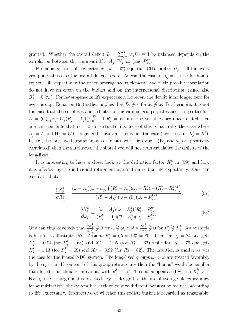
granted. Whether the overall deficit D =∑J

j=1 πjDj will be balanced depends on the

correlation between the main variables Aj, Wj, ωj (and R∗j ).

For homogeneous life expectancy (ωj = ω) equation (61) implies Dj = 0 for every

group and thus also the overall deficit is zero. As was the case for ηj = 1, also for homo-

geneous life expectancy the other heterogeneous elements and their possible correlation

do not have an effect on the budget and on the interpersonal distribution (since also

Bkj = 0,∀k). For heterogeneous life expectancy, however, the deficit is no longer zero for

every group. Equation (61) rather implies that Dj R 0 for ωj R ω. Furthermore, it is not

the case that the surpluses and deficits for the various groups just cancel. In particular,

D =∑J

j=1 πjτWj(R∗j − Aj)

ωj−ωω−R∗j

. If R∗j = R∗ and the variables are uncorrelated then

one can conclude that D = 0 (a particular instance of this is naturally the case where

Aj = A and Wj = W ). In general, however, this is not the case (even not for R∗j = R∗).

If, e.g., the long-lived groups are also the ones with high wages (Wj and ωj are positively

correlated) then the surpluses of the short-lived will not counterbalance the deficits of the

long-lived.

It is interesting to have a closer look at the deduction factor Xkj in (59) and how

it is affected by the individual retirement age and individual life expectancy. One can

calculate that:

∂Xkj

∂Rkj

=(ω − Aj)(ω − ωj)

((R∗j − Aj)(ωj −R∗j ) + (R∗j −Rk

j )2)

(Rkj − Aj)2(ω −R∗j )(ωj −Rk

j )2

, (62)

∂Xkj

∂ωj=

(ω − Aj)(ω −Rkj )(R

∗j −Rk

j )

(Rkj − Aj)(ω −R∗j )(ωj −Rk

j )2. (63)

One can thus conclude that∂X

kj

∂Rkj

R 0 for ω R ωj while∂X

kj

∂ωjR 0 for R∗j R Rk

j . An example

is helpful to illustrate this. Assume R∗j = 65 and ω = 80. Then for ωj = 84 one gets

Xkj = 0.94 (for Rk

j = 68) and Xkj = 1.05 (for Rk

j = 62) while for ωj = 76 one gets

Xkj = 1.13 (for Rk

j = 68) and Xkj = 0.92 (for Rk

j = 62). The intuition is similar as was

the case for the biased NDC system. The long-lived groups ωj > ω are treated favorably

by the system. If someone of this group retires early then the “bonus” would be smaller

than for the benchmark individual with Rkj = R∗j . This is compensated with a Xk

j > 1.

For ωj < ω the argument is reversed. By its design (i.e. the use of average life expectancy

for annuitization) the system has decided to give different bonuses or maluses according

to life expectancy. Irrespective of whether this redistribution is regarded as reasonable,

63

the retirement age should not have an affect on the amount of these transfers. This is

achieved by the use of Xkj .

In reality, NDC systems typically use average life expectancy for calculating the annu-

ity but I know of no system that in fact has implemented a corrective deduction factor like

Xkj in equation (59). It is thus interesting to look at the consequences if a NDC system

just uses the basic formula P kj = τWj

Rkj−Ajω−Rkj

without an additional Xkj . Straightforward

calculations show that the bonus is in this case Bkj = τWj(R

kj − Aj)

ωj−ωω−Rkj

. This has the

following implications. First, the overall deficit Dj of group j is no longer independent

of the retirement behavior. This only holds (approximately) true if R∗j = Rj. This,

however, cannot be taken for granted. In particular, it implies that the retirement age

is not correlated with lifetime wages, entry age and life expectancy which is implausible.

Second, different to (60) now the bonus is not the same for every member k of group j.

Rather it holds that∂B

kj

∂ωj> 0 (long-lived get higher bonuses) and

∂Bkj

∂Rkj

R 0 for ωj R ω. It

is not clear whether this is a desired consequence. An early retiree among the long-lived

will now get a smaller bonus than before (which might be an appreciated consequence),

but a long-lived late retiree will be rewarded with an even larger bonus (which looks less

favorable). On the other hand, the early short-lived retiree has a smaller disadvantage

than with the use of Xkj (which might be regarded as positive) but the late retirees among

the short-lived get a larger punishment.

D.3 Pension adjustment with inflation (section 5.3)

I have assumed in the model of appendix C that ongoing pensions are adjusted with the

rate of growth (ϑ(t) = g(t)) as shown in equation (34). In reality there exist different

adjustment regimes and while some countries use growth rate of average wages for ad-

justment others refer to the growth rate of the wage sum, the rate of inflation or mixtures

of these concepts. It is thus interesting to study the implications of different adjustment

regimes. I focus on the case where pensions are held constant in real terms, i.e. where

they are are only indexed to the rate of inflation and thus ϑ(t) = 0. For the NDC system

this means that:

PNDC(R, a, t) = PNDC(R,R, t) = ητW (t+R)(R− A)h(R)

e(R)= ητW (t+R)

∫ RAS(a) da∫ ω

RS(a) da

,

where I allow for an additional multiplier η to the “pure” NDC pension as discussed above

in section D.1. For the benchmark case with R = R∗ one gets that I∗ = τW (t)∫ R∗AS(a) da

64

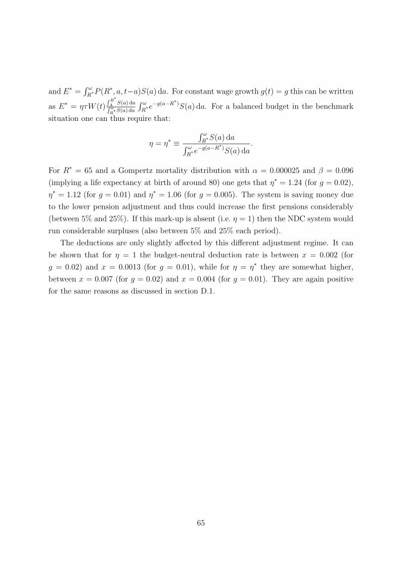
and E∗ =∫ ωR∗P (R∗, a, t−a)S(a) da. For constant wage growth g(t) = g this can be written

as E∗ = ητW (t)∫R∗A S(a) da∫ ωR∗S(a) da

∫ ωR∗e−g(a−R

∗)S(a) da. For a balanced budget in the benchmark

situation one can thus require that:

η = η∗ ≡∫ ωR∗S(a) da∫ ω

R∗e−g(a−R

∗)S(a) da

.

For R∗ = 65 and a Gompertz mortality distribution with α = 0.000025 and β = 0.096

(implying a life expectancy at birth of around 80) one gets that η∗ = 1.24 (for g = 0.02),

η∗ = 1.12 (for g = 0.01) and η∗ = 1.06 (for g = 0.005). The system is saving money due

to the lower pension adjustment and thus could increase the first pensions considerably

(between 5% and 25%). If this mark-up is absent (i.e. η = 1) then the NDC system would

run considerable surpluses (also between 5% and 25% each period).

The deductions are only slightly affected by this different adjustment regime. It can

be shown that for η = 1 the budget-neutral deduction rate is between x = 0.002 (for

g = 0.02) and x = 0.0013 (for g = 0.01), while for η = η∗ they are somewhat higher,

between x = 0.007 (for g = 0.02) and x = 0.004 (for g = 0.01). They are again positive

for the same reasons as discussed in section D.1.

65

Index of Working Papers: March 5, 2015

Jonas Dovern, Martin Feldkircher, Florian Huber

200 Does Joint Modelling of the World Economy Pay Off? Evaluating Global Forecasts from a Bayesian GVAR

May 19, 2015

Markus Knell

201 The Return on Social Security with Increasing Longevity

June 15, 2015

Anil Ari

202 Sovereign Risk and Bank Risk-Taking

June 15, 2015

Matteo Crosignani

203 Why Are Banks Not Recapitalized During Crises?

February 19, 2016

Burkhard Raunig

204 Background Indicators

February 22, 2016

Jesús Crespo Cuaresma, Gernot Doppelhofer, Martin Feldkircher, Florian Huber

205 US Monetary Policy in a Globalized World

March 4, 2016

Helmut Elsinger, Philipp Schmidt-Dengler, Christine Zulehner

206 Competition in Treasury Auctions

May 14, 2016

Apostolos Thomadakis

207 Determinants of Credit Constrained Firms: Evidence from Central and Eastern Europe Region

July 1, 2016

Martin Feldkircher, Florian Huber

208 Unconventional US Monetary Policy: New Tools Same Channels?

November 24, 2016

François de Soyres 209 Value Added and Productivity Linkages Across Countries

November 25, 2016

Maria Coelho 210 Fiscal Stimulus in a Monetary Union: Evidence from Eurozone Regions

January 9, 2017

Markus Knell, Helmut Stix

211 Inequality, Perception Biases and Trust

January 31, 2017

Steve Ambler, Fabio Rumler

212 The Effectiveness of Unconventional Monetary Policy Announcements in the Euro Area: An Event and Econometric Study

May 29, 2017

Filippo De Marco 213 Bank Lending and the European Sovereign Debt Crisis

June 1, 2017

Jean-Marie Meier 214 Regulatory Integration of International Capital Markets

October 13, 2017

Markus Knell 215 Actuarial Deductions for Early Retirement