working paper 01-2 departamento de estadística y ... · working paper 01-2 departamento de...
TRANSCRIPT

Working Paper 01-2 Departamento de Estadística y EconometríaStatistics and Econometrics Series 1 Universidad Carlos III de MadridJanuary 2001 Calle Madrid, 126
28903 Getafe (Spain)Fax (34-91) 624-9849
IMPROVED NONPARAMETRIC CONFIDENCE INTERVALS IN TIME SERIESREGRESSIONS
Joseph P. Romano and Michael Wolf*
Abstract __________________________________________________________________Confidence intervals in time series regressions suffer from notorious coverage problems.
This is especially true when the dependence in the data is noticeable and sample sizes are
small to moderate, as is often the case in empirical studies. This paper proposes a method
that combines prewhitening and the studentized bootstrap. While both prewhitening and the
studentized bootstrap each provides improvement over standard normal theory intervals,
one can achieve a further improvement by conjoining them in an appropriate way. As a side
note, it is stressed that symmetric confidence intervals equal-tailed ones, since they exhibit
improved coverage accuracy. We propose concrete ways to deal with the issues of block
size, choice of kernel, and choice of bandwidth. The improvements in small sample
performance are supported by a simulation study.
_________________________________________________________________________
Keywords: Bootstrap; confidence intervals; studentization; time series regressions;prewhitening.
*Romano, Department of Statistics, Stanford University, Stanford, CA 94305, U.S.A.,Phone: 650-7236326, e-mail: [email protected]. Wolf, Departamento deEstadística y Econometría, Universidad Carlos III de Madrid. C/ Madrid, 126 28903Madrid. Spain. Ph: 34-91-624.98.63, Fax: 34-91-624.98.49, e-mail: [email protected]; Research of the first author funded by the National Science Foundation,DMS 9704487. Research of the second author partly funded by the Spanish “DirecciónGeneral de Enseñanza Superior” (DGES), reference number PB98-0025.

Improved Nonparametric Con�dence Intervals in Time Series
Regressions
Joseph P. Romano �
Department of Statistics
Stanford University
Stanford, CA 94305, U.S.A.
Michael Wolf
Departamento de Estad��stica y Econometr��a
Universidad Carlos III de Madrid
28903 Getafe, SPAIN
Working Paper 01-2, Statistics and Econometrics Series 1, January 2001
Abstract
Con�dence intervals in time series regressions su�er from notorious coverage prob-
lems. This is especially true when the dependence in the data is noticeable and sample
sizes are small to moderate, as is often the case in empirical studies. This paper pro-
poses a method that combines prewhitening and the studentized bootstrap. While both
prewhitening and the studentized bootstrap each provides improvement over standard
normal theory intervals, one can achieve a further improvement by conjoining them in
an appropriate way. As a side note, it is stressed that symmetric con�dence intervals
equal-tailed ones, since they exhibit improved coverage accuracy. We propose concrete
ways to deal with the issues of block size, choice of kernel, and choice of bandwidth.
The improvements in small sample performance are supported by a simulation study.
JEL CLASSIFICATION NOS: C14, C15, C22, C32.
KEY WORDS: Bootstrap, Con�dence Intervals, Studentization, Time Series Regressions,
Prewhitening.
�Joseph P. Romano, Phone: (650) 723-6326, Fax: (650) 725-8977, E-mail: [email protected].
Research of the �rst author funded by the National Science Foundation, DMS 9704487; Research of the
second author partly funded by the Spanish \Direcci�on General de Ense~nanza Superior" (DGES), reference
number PB98-0025.

1 Introduction
Regressions in macroeconomics and �nance typically involve explanatory variables and/or
error variables that exhibit serial dependence. It is well-known that standard regression
theory does not apply to such settings but appropriate asymptotic theory for time series
regression has been developed and is routinely applied in practice; for example, see Hannan
(1970) or White (1984). Over the last decade, the literature has shown that the �nite
sample properties of standard (or normal theory) methods are often lacking in practice;
a common phenomenon is that con�dence intervals undercover and that hypothesis tests
overreject. We will focus on the construction of con�dence intervals in the remainder of the
paper; however, the ideas also apply to hypothesis tests.
A number of recent proposals have been made to construct con�dence intervals that
exhibit improved coverage accuracy. The two most common proposals, arguably, are
prewhitening (Andrews and Mohanan, 1992; Newey and West, 1994) and bootstrapping
(Fitzenberger, 1997). As far as the bootstrap is concerned, it seems that the importance
of using a studentized bootstrap in order to achieve asymptotic re�nements over normal
theory has not yet been realized in the time series regression literature. This importance, in
the context of smooth functionals of the mean, was pointed out by Davison and Hall (1993)
and G�otze and K�unsch (1996).
We propose a new approach which combines prewhitening and the studentized bootstrap
to yield an even further improvement. Previous theory suggests that both prewhitening and
the use of a studentized bootstrap each o�ers improved coverage properties. By combining
these two approaches and o�ering concrete suggestions on implementation (such as choice of
block size, kernel, and bandwidth parameters), we believe we provide a useful method that
is safe to apply in practice. Formal theory would require tedious and lengthy Edgeworth
expansions, and even in i.i.d. situations, typically only provide rates of convergence for
coverage error and length of intervals. Although such theory lends theoretical support in
our fairly complicated time series regression setting, we validate our claims by heuristics
and a simulation study, with theoretical work to follow. In addition, it is stressed that
when two-sided con�dence intervals are to be constructed, one should employ symmetric
intervals as opposed to equal-tailed intervals, since the former tend to enjoy better coverage
properties.
The remainder of the paper is organized as follows. Section 2 presents the model and
the inference problem. In Section 3 some previous methods are brie y reviewed. Section 4
gives the details of our method. We also discuss how to choose the block size which is
an important model parameter of any nonparametric time series bootstrap. Finite sample
performance is examined via a simulation study in Section 5. Finally, Section 6 summarizes
our �ndings. All tables appear in Section 7 at the end of the paper.
1

2 The Model
We consider the following regression model
yt = X0
t� + �t; t = 1; : : : ; T; (1)
where � 2 RI p. The ordinary least squares (OLS) estimator for � is given by
�T =
TXt=1
XtX0
t
!�1 TXt=1
Xtyt:
A critical assumption to ensure its consistency is E(Xt�t) = 0; t = 1; : : : ; T; that is, the
regressors are uncorrelated with the error term. This assumption is typically implied by
economic considerations, such as a rational expectation model. Another key assumption is
a weak dependence condition on the f(X 0
t; �t)0g process. We assume an �-mixing condition,
which is standard in the literature; for example, see White (1984). Alternatively, other weak
dependence conditions could be employed. Finally, some moment conditions on the fX 0
t�tgand f�tg processes and some heteroscedasticity bounds are needed to ensure asymptotic
normality of the OLS estimator �T . For detailed su�cient sets of mixing, moments, and
heteroscedasticity bounds conditions, the reader is referred to White (1984, Chapter V) or
Politis et al. (1999, Theorem 3.4), among others. One of such sets shall be assumed in
the sequel of the paper. Note that our method will generally not work under nonstandard
asymptotics, one example being the situation where one of the regressors has a unit root.
Interest focuses on constructing con�dence intervals for a real-valued parameter � = a0�,
where a is a �xed and known p�1 vector. Quite often � will simply be a particular regressioncoe�cient of interest. The restriction to real-valued parameters is made mainly to give a
natural setting for the construction of con�dence intervals. Of course, other parameters can
be considered as well. For example, one might be interested in a general linear function R�,
where R is a �xed and known l�p matrix, an important special case being R = Ip, the p�pidentity matrix. If the parameter of interest is multivariate, one often uses hypothesis tests,
since it is somewhat di�cult to explicitly write down a multivariate con�dence region. The
method proposed can be easily adapted to testing problems; see Remark 4.1.
3 Background
In this section, two previous approaches for making inference in time series regressions are
reviewed. Some details are presented that will be relevant later on.
3.1 Normal Theory
Under nonrestrictive regularity conditions,pT (�T ��)
L
=) N(0;�), where � is a positive-
de�nite p� p matrix andL
=) denotes convergence in distribution (or convergence in law).
2

This impliespT (a0�T � �)
L
=) N(0; a0�a), which would allow one to construct an asymp-
totic normal theory con�dence interval for � if � were known. Unfortunately, � depends
on the unknown underlying probability mechanism. The standard way of making inference
is therefore to consistently estimate the limiting covariance matrix � by an estimator �T
and to pretend the distribution ofpT (a0�T � �) is given by N(0; a0�Ta), that is, to use the
plug-in principle. As is well-known,
� = limT!1
1
T
TXt=1
XtX0
t
!�11
T
TXs=1
TXt=1
E�sXs(�tXt)0
1
T
TXt=1
XtX0
t
!�1:
Since the series fXtg is observed, consistent estimation of � only requires a consistent
estimator of JT � (1=T )PT
s=1
PTt=1E�sXs(�tXt)
0. By change of variables, and introducing
the notation Vt = �tXt, the estimand JT can be rewritten as
JT =T�1X
j=�T+1
�T (j) + �T (j)0;
where
JT =
(�T (j) =
1T
PTt=j+1EVtVt�j if j � 0
�T (j) =1T
PTt=�j+1EVt+jVt if j < 0:
A natural estimator for �T (j) is given by
�T (j) =1
T
TXt=j+1
VtVt�j ; where Vt = Xt(yt �X0
t�T ):
Unfortunately, simply replacing �T (j) by �T (j) in the formula for JT would lead to an
inconsistent estimator; for example, see Priestley (1981, Chapter 6). The most common
way to arrive at consistent estimators for JT is to consider kernel estimators of the form
JT = JT (ST ) =T
T � p
T�1Xj=�T+1
k
�j
ST
��T (j); (2)
yielding
�T =
1
T
TXt=1
XtX0
t
!�1JT
1
T
TXt=1
XtX0
t
!�1: (3)
In (2), k(�) is a real-valued kernel, ST is a bandwidth parameter, and the factor T=(T �p) isa small-sample-degree-of-freedom adjustment for estimating the p-dimensional parameter �.
The kernel k(�) determines the weight that is given to the �T (j) and typically satis�es the
three conditions k(0) = 1, k(�) is continuous at 0, and limx!�1 k(x) = 0. For a number of
popular kernels, see Priestley (1981, Chapter 6) or Andrews (1991), among others.
An important feature of a kernel is its characteristic exponent 1 � q � 1, determined
by the smoothness of the kernel at the origin. Note that the bigger q, the smaller is the
asymptotic bias of a kernel variance estimator; on the other hand, only kernels with q � 2
3

yield estimates that are guaranteed to be positive semi-de�nite in �nite samples. Most of
the commonly used kernels have q = 2, such as the Parzen, Tukey-Hanning, and Quadratic-
Spectral (QS) kernels, while the Bartlett kernel has q = 1 and the Truncated kernel has
q =1. For a broader discussion on this issue, see Priestley (1981, Chapter 6).
Once a particular kernel k(�) has be chosen for application, one is left to pick the
bandwidth ST . Several data-dependent methods, based on various asymptotic optimality
criteria, are available to choose ST ; for example, see Andrews (1991) and Newey and West
(1994). Note that the `optimal' bandwidth generally depends on the underlying stochastic
mechanism generating the data, as well as the choice of the kernel k(�).
Given the kernel estimator JT , it is now straightforward to compute the estimator �T
and construct normal theory con�dence intervals for � as outlined above. However, these
intervals tend to work unsatisfactorily in small samples, especially when the dependence
structure of the underlying data is strong; again, see Andrews (1991) and Newey and West
(1994). The method of prewhitening, dating back to Press and Tukey (1956), has been
suggested to better this situation and it works as follows. It is well-known that covariance
matrix estimation corresponds to spectral density matrix estimation at frequency zero and
that it is easier to estimate spectral density matrices of white noise processes than those of
heavily dependent processes. The idea then is to �rst transform the fVtg process to make
it look more like white noise (that is, to prewhiten it), to then estimate the spectral density
matrix of the transformed process at frequency zero, and to �nally recolor the estimated
matrix. The transformation is usually done by passing the fVtg process through a linear
�lter, often taken to be a Vector Autogressive (VAR) model, and the recoloring is achieved
by applying the inverse transformation to the estimated spectral density matrix of the
�ltered process. To be more speci�c, �rst, one estimates a dth order VAR model (by OLS,
say) for Vt:
Vt =dX
r=1
ArVt�r + Ut:
Second, one computes a standard covariance matrix estimator, call it J UT , as described above
but based on the VAR residual vectors fUtg rather than the original vectors fVtg. Third,one recolors J UT to obtain a prewhitened estimator of JT :
JT;PW = DJUT D
0; where D =
Ip �
dXr=1
Ar
!�1; (4)
yielding
�T;PW =
1
T
TXt=1
XtX0
t
!�1JT;PW
1
T
TXt=1
XtX0
t
!�1: (5)
Note that the matrix (Ip �Pd
r=1 Ar) in (4) may not be invertible, in which case a general
inverse can be used or an invertibility adjustment (e.g., Andrews and Monahan, 1992) can
be made to compute D. Instead of VAR models, other linear �lters could be used in the
prewhitening and recoloring process.
4

According to empirical studies in Andrews and Monahan (1992) and Newey and West
(1994), among others, con�dence intervals for � based on �T;PW tend to exhibit better
coverage properties in �nite samples than those based on �T .
3.2 The Bootstrap
Given the success of the bootstrap in regression settings with independent observations (Wu,
1986), it is natural to apply an appropriate bootstrap method to time series regressions.
Such a method has to take into account the time series structure of both the regressors
and the error variables. In the absence of semi-parametric structural models for these
variables, such as AR or VAR models with i.i.d. innovations, the common approach is
to resample blocks of data. For ease of notation, let Zt = (X 0
t; yt)0, so the observed data
is fZ1; : : : ; ZT g; also denote the true probability mechanism by P . The most popular
time series bootstrap is the moving blocks bootstrap due to K�unsch (1989) and Liu and
Singh (1992). It considers overlapping blocks of size b, namely Yt = fZt; : : : ; Zt+b�1g,t = 1; : : : ; T � b + 1. Assuming for the moment T = lb, the method selects l blocks Y �t
at random and with replacement from the T � b + 1 available blocks and concatenates
them to arrive at the pseudo sequence fY �1 ; : : : ; Y �l g = fZ�1 ; : : : ; Z�T g; in case T is not
a multiple of b, one would do the same with the smallest l such that T < lb and then
truncate the pseudo sequence at T observations. Denote by P �T the bootstrap distribution
(conditional on the observed data) of the pseudo sequence fZ�1 ; : : : ; Z�T g. Let ��T be the OLS
estimator of � computed from the pseudo sequence and let ��T be the corresponding linear
combination a0��T . A straightforward bootstrap approximation of the sampling distribution
of the OLS estimator �T is then
LPf�T � �g � LP �
Tf��T � �T g: (6)
Here, the general notation LQfWg stands for the law of a random variable W when the
probability mechanism is Q.
The relation (6) can now be used to construct an approximate con�dence interval for �.
This particular bootstrap approximation is usually referred to as the hybrid bootstrap (Hall,
1992) or the basic bootstrap (Davison and Hinkley, 1997); we shall use the latter notation
henceforth. Two problems with the moving blocks bootstrap are that it does not produce
stationary pseudo sequences even if the original sequence is stationary and that �T generally
is not equal to �(P �T ), the parameter � corresponding to the bootstrap distribution P �T , due
to `edge e�ects'. To �x these shortcomings, Politis and Romano (1994) suggested the
stationary bootstrap where the data are `wrapped' in a circle and the block lengths are
random i.i.d. according to a geometric distribution. The result are bootstrap sequences
that are stationary and avoid edge e�ects.
Fitzenberger (1997) applied the basic moving blocks bootstrap to time series regressions.
However, its �nite sample performance did not appear superior to normal theory intervals.
5

The reason for this `disappointment' has its roots in the much-studied simpler setting of
the mean for i.i.d. observations. It is well-known (e.g., Hall, 1992) that, in this setting, the
basic bootstrap does not provide an asymptotic re�nement over the CLT normal interval
in the sense that both are only �rst order correct. To achieve second order correctness,
a more sophisticated method such as the studentized or the BCa bootstrap has to be
employed. This result carries over to the dependent case. Davison and Hall (1993) and
G�otze and K�unsch (1996), abbreviated by DH and GK, respectively, in the remainder of
this paper, considered inference for the mean (and smooth functions of the mean) in the
context of stationary, dependent observations. They showed that the basic bootstrap is
only �rst order correct while the studentized bootstrap provides an asymptotic re�nement,
at least under regularity conditions that ensure an Edgeworth expansion; detailed sets of
such conditions can be found in DH and GK. Note that it turns out to be important
that the studentization is done in a certain way; see the discussion below. Moreover,
the moving blocks bootstrap distribution needs to be centered around the mean of the
bootstrap distribution rather than the sample mean. Unfortunately, the theory covering
the mean case for dependent data, based on nontrivial Edgeworth expansions, is already
very complicated, so that a corresponding result for time series regressions would be lengthy
and quite technical. However, since the mean is a special case of an OLS estimator, it is
natural to expect better performance from a studentized bootstrap in general regression
settings as well.
The studentized bootstrap, together with the proper centering, leads to the approxima-
tion
LPf(�T � �)=�T g � LP �
Tf(��T � �(P �T ))=�
�
T g; (7)
which again can be used to construct a con�dence interval for �. Here, �T is an estimator of
the standard deviation of �T and ��T is an estimator of the standard deviation of ��T . Often,
and also in the particular method that we will suggest in Section 4, the two estimators have
the same form, one being applied to the original sequence and the other being applied to
the bootstrap sequence. A natural choice for our application is a kernel estimator and then
�T =
qa0�Ta and �
�
T =qa0��Ta. In the latter expression, ��T is the kernel estimator of �
applied to the bootstrap sequence.
Remark 3.1 In certain instances the forms of �T and ��
T may be di�erent. For example,
when the bootstrap sequence is generated by the moving blocks bootstrap, one can exploit
the particular dependence structure of such a sequence (it being generated by concatenating
i.i.d. blocks of data) to arrive at the following `natural' variance estimator ��T (DH and GK):
Assuming for simplicity that T = lb, where b is the block size used to construct the moving
blocks bootstrap sequence, de�ne
V�
t = X�
t (y�
t �X�
t ��
T ); t = 1; : : : ; T;
�j =1pb
bXt=1
V�
(j�1)b+t; j = 1; : : : ; l;
6

and
��T;MB =
1
T
TXt=1
X�
t (X�
t )0
!�11
l
lXj=1
(�j � ��)2 1
T
TXt=1
X�
t (X�
t )0
!�1:
Then, the `natural' variance estimator is given by
��
T =qa0��T;MBa: (8)
On the other hand, DH and GK suggest to use a kernel estimator based on the Truncated
kernel for the choice of �T .
The reasoning for choosing di�erent forms of �T and ��
T in this context is as follows.
DH and GK showed that in order to obtain asymptotic re�nements over normal theory
it is crucial to use low bias variance estimators in the studentization. They then picked
the variance estimators with smallest bias for both the original time series as well as the
bootstrap generated time series. With this choice, the bootstrap approximation (7) can be
shown to have error OP (n�3=4+�) where � is a small number (DH and GK); in contrast, the
approximation (6) has error larger than OP (n�1=2) as does normal theory.
Remark 3.2 An issue that arises when two-sided bootstrap con�dence intervals are desired
is whether to construct equal-tailed or symmetric intervals; note that normal theory intervals
are both equal-tailed and symmetric by nature. In the setting of independent data and
under appropriate regularity conditions, it has been repeatedly pointed out that symmetric
bootstrap con�dence intervals enjoy improved coverage accuracy (e.g., Beran, 1987; Hall,
1988). Such considerations carry over to dependent data settings. Hence, if coverage is
of prime concern, it is preferable to construct symmetric intervals based on the bootstrap
approximation of the two-sided sampling distribution function
LPfj�T � �j=�(�T )g � LP �
Tfj��T � �(P �T )j=��(��T )g:
4 Studentization with a Prewhitened Kernel Variance Esti-
mator
4.1 The General Method
The previous section presented two approaches to improve upon standard normal theory
intervals, namely using a prewhitened kernel estimator to construct normal theory inter-
vals, and employing a studentized bootstrap. It is an obvious idea to combine these two
approaches to obtain an even further improvement. The method is simple and consists of
using a studentized bootstrap in conjunction with a prewhitened kernel variance estimator.
Consider the general studentized bootstrap approximation (7). As outlined in Re-
mark 3.1, DH and GK use a di�erent studentization for the bootstrap sequence as compared
7

to the original sequence in order to get variance estimators with minimal variance in both
worlds. However, a closer inspection of the proofs of DH and GK reveals that �T and ��
T
can be taken to be of the same form and an asymptotic re�nement over the normal approx-
imation still be retained. Indeed, if the (common) variance estimator is based on a kernel
with characteristic component q = 2, an error of OP (n�2=3+�) is achieved.
Given that the method of DH and GK has an error of OP (n�3=4+�), why do we suggest
to use a common variance estimator? There are two reasons. First, and less importantly,
the Truncated kernel used by DH and GK in computing �T can lead to negative variance
estimates in �nite samples. By using a kernel with characteristic component q = 2 this
problem is avoided. Second, we expect to improve upon DH and GK by using a com-
mon prewhitened kernel variance estimator. A corresponding theoretical result would be
extremely technical and would seem to have to be limited to certain classes of probability
mechanisms. Rather, along the lines of Andrews and Monahan (1992) and Newey and West
(1994), we shall promote our method by heuristic arguments combined with simulation ev-
idence. Heuristics say that prewhitened kernel variance estimators tend to perform better
than standard kernel variance estimators and this edge should carry over to the studentized
bootstrap. The simulation evidence will be presented in Section 5.
For the implementation of the method, one must choose a prewhitened kernel variance
estimator and a suitable time series bootstrap. As far as the kernel is concerned, it was
seen necessary to employ a kernel with q � 2 to achieve asymptotic re�nements. On the
other hand, only a kernel with q � 2 is guaranteed to yield positive semi-de�nite variance
estimates in �nite samples. We therefore suggest a kernel with q = 2. Among these, the
so-called Quadratic Spectral (QS) kernel enjoys some attractive optimality properties; for
example, see Priestley (1983, Chapter 6) or Andrews (1991). We shall use this kernel in the
remainder of the paper.
As for a suitable bootstrap method, it is clear that a generally valid time series bootstrap
needs to be employed. In the absence of a plausible (semi-)parametric data generating
mechanism, a nonparametric method should be employed. Natural choices are the moving
blocks bootstrap and the stationary bootstrap. We propose the latter for two reasons. First,
due to the avoidance of `edge e�ects', one has �(P �T ) = �T for the stationary bootstrap while
for the moving blocks bootstrap the parameter of the bootstrap distribution would require
an extra computation. Second, both bootstrap methods depend on a model parameter
that governs the block size but the stationary bootstrap appears less sensitive to its choice
(Politis and Romano, 1994; Davison and Hinkley, 1997, Section 8.2).
Remark 4.1 We have proposed a method to construct con�dence intervals for a real-
valued parameter � = a0�, where a is a �xed known p� 1 vector. At times, interest might
instead focus on a multivariate parameter � = R�, where R is a �xed and known l � p
matrix. In this instance, it is more natural to consider hypothesis tests of the sort H0 :
R� = r0, since multivariate con�dence regions are somewhat di�cult to write down. Note
8
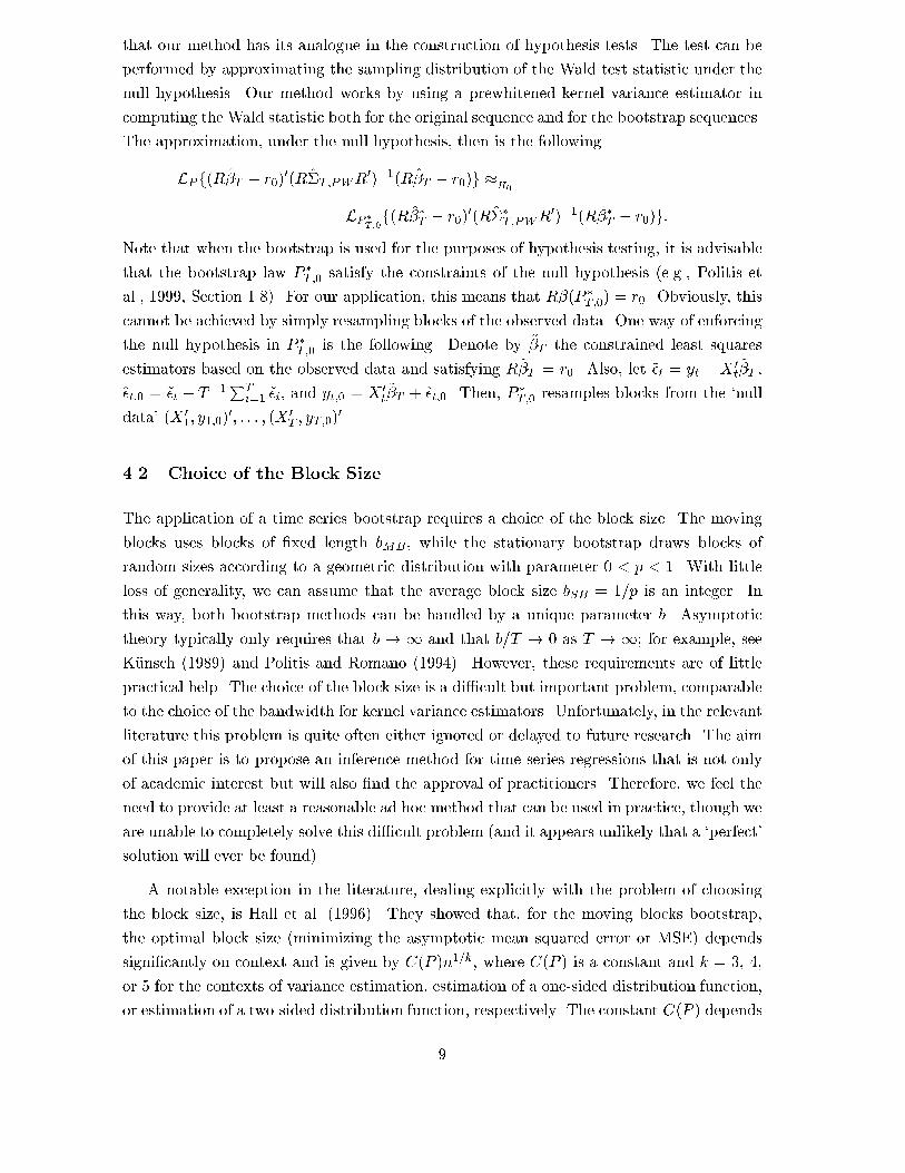
that our method has its analogue in the construction of hypothesis tests. The test can be
performed by approximating the sampling distribution of the Wald test statistic under the
null hypothesis. Our method works by using a prewhitened kernel variance estimator in
computing the Wald statistic both for the original sequence and for the bootstrap sequences.
The approximation, under the null hypothesis, then is the following
LP f(R�T � r0)0(R�T;PWR
0)�1(R�T � r0)g �H0
LP �
T;0f(R��T � r0)
0(R��T;PWR0)�1(R��T � r0)g:
Note that when the bootstrap is used for the purposes of hypothesis testing, it is advisable
that the bootstrap law P�
T;0 satisfy the constraints of the null hypothesis (e.g., Politis et
al., 1999, Section 1.8). For our application, this means that R�(P �T;0) = r0. Obviously, this
cannot be achieved by simply resampling blocks of the observed data. One way of enforcing
the null hypothesis in P�
T;0 is the following. Denote by ~�T the constrained least squares
estimators based on the observed data and satisfying R ~�T = r0. Also, let ~�t = yt �X0
t~�T ,
~�t;0 = ~�t � T�1PT
i=1 ~�i, and yt;0 = X0
t~�T + ~�t;0. Then, P
�
T;0 resamples blocks from the `null
data' (X 0
1; y1;0)0; : : : ; (X 0
T ; yT;0)0.
4.2 Choice of the Block Size
The application of a time series bootstrap requires a choice of the block size. The moving
blocks uses blocks of �xed length bMB, while the stationary bootstrap draws blocks of
random sizes according to a geometric distribution with parameter 0 < p < 1. With little
loss of generality, we can assume that the average block size bSB = 1=p is an integer. In
this way, both bootstrap methods can be handled by a unique parameter b. Asymptotic
theory typically only requires that b ! 1 and that b=T ! 0 as T ! 1; for example, see
K�unsch (1989) and Politis and Romano (1994). However, these requirements are of little
practical help. The choice of the block size is a di�cult but important problem, comparable
to the choice of the bandwidth for kernel variance estimators. Unfortunately, in the relevant
literature this problem is quite often either ignored or delayed to future research. The aim
of this paper is to propose an inference method for time series regressions that is not only
of academic interest but will also �nd the approval of practitioners. Therefore, we feel the
need to provide at least a reasonable ad hoc method that can be used in practice, though we
are unable to completely solve this di�cult problem (and it appears unlikely that a `perfect'
solution will ever be found).
A notable exception in the literature, dealing explicitly with the problem of choosing
the block size, is Hall et al. (1996). They showed that, for the moving blocks bootstrap,
the optimal block size (minimizing the asymptotic mean squared error or MSE) depends
signi�cantly on context and is given by C(P )n1=k, where C(P ) is a constant and k = 3, 4,
or 5 for the contexts of variance estimation, estimation of a one-sided distribution function,
or estimation of a two-sided distribution function, respectively. The constant C(P ) depends
9

on the underlying joint distribution P and the context but a way is suggested to estimate it
in practice. The problem with trying to adopt their approach for our purposes is two-fold.
First, all the asymptotic MSE calculations are done for the basic moving blocks bootstrap
and thus would no longer be valid for the studentized moving blocks bootstrap. Second, for
the estimation of a distribution function, C(P ) depends on the argument of that function,
that is, on x in F (x) = ProbPfZ � xg for a general random variable Z. Since our interest is
in estimating a quantile of a distribution function, it seems that the corresponding x would
�rst have to be found in some recursive fashion.
Instead, we will propose a method which can be applied to an arbitrary bootstrap
method, whether studentized or not, and which immediately tackles the task of estimating a
speci�c quantile as opposed to estimating the distribution function at a given point. To this
end, we suggest to use a calibration method, a concept dating back to Loh (1987, 1988, 1991).
One can think of the actual coverage level 1�� of a time series bootstrap con�dence interval
as a function of the block size b, conditional on the underlying probability mechanism P ,
the nominal con�dence level 1 � �, and the sample size T . The idea is now to adjust the
`input' b in order to obtain the actual coverage level close to the desired one. Hence, one
can consider the block size calibration function g : b! 1��. If g(�) were known, one couldconstruct an `optimal' con�dence interval by �nding ~b that minimizes jg(b) � (1 � �)j anduse ~b as the block size of the time series bootstrap; note that jg(b) � (1 � �)j = 0 may not
always have a solution.
Of course, the function g(�) depends on the underlying probability mechanism P and is
therefore unknown. We now propose a semi-parametric bootstrap method to estimate it.
The idea is that in principle we could simulate g(�) if P were known by generating data of
size T according to P and computing con�dence intervals for � for a number of di�erent
block sizes b. This process is then repeated many times and for a given b one estimates g(b)
as the fraction of the corresponding intervals that contain the true parameter. The method
we propose is identical except that P is replaced by a semi-parametric estimate PT .
Algorithm 4.1 (Choice of the Block Size)
1. Fit a semi-parametric model PT to the observed data (X 0
1; y1)0; : : : ; (X 0
T ; yT )0.
2. Fix a selection of reasonable block sizes b.
3. Generate K pseudo sequences ((X�
1 )0; y�
1)0
k : : : ; ((X�
T )0; y�
T )0
k, k = 1; : : : ;K, according
to PT . For each sequence, k = 1; : : : ;K, and for each b, compute a con�dence interval
CIk;b.
4. Compute g(b) = #f�(PT ) 2 CIk;bg=K.
5. Find the value of ~b that minimizes jg(b)� (1� �)j.
10
The choice of a semi-parametric model rather than a nonparametric time series bootstrap
in generating the pseudo sequences is motivated by the fact that the latter would require
a block size of its own. The role of the semi-parametric model in Algorithm 4.1 can be
compared to the role of the semi-parametric model in the prewhitening for kernel variance
estimation. Even if the model is misspeci�ed, it should contain some information on the
dependence structure of the true mechanism P that can be exploited to estimate g(�). In
practice we suggest to employ a VAR model, whose order could be estimated by one of
the well-known information criteria, say, in conjunction with bootstrapping the estimated
residuals.
Remark 4.2 Note that Algorithm 4.1 is essentially a double bootstrap and therefore com-
putationally more expensive, by an order of magnitude, than the application of the bootstrap
method once the block size has been determined.
Remark 4.3 If a bootstrap method is used for hypothesis testing rather than con�dence
interval construction, an analogous algorithm can be used by focusing on the signi�cance
level of the test rather than on the con�dence level of the interval. Note that in this case
the semi-parametric model PT should be replaced by a semi-parametric model PT;0 which
satis�es the constraints of the the null hypothesis; the remaining details are straightforward.
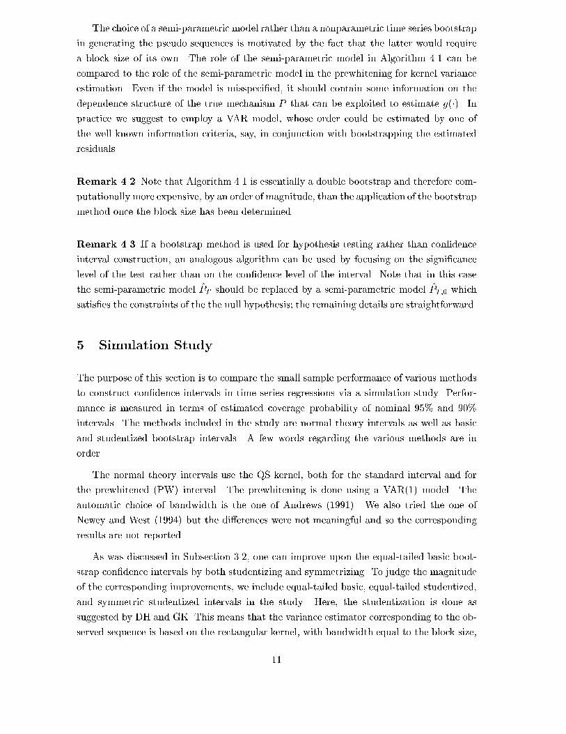
5 Simulation Study
The purpose of this section is to compare the small sample performance of various methods
to construct con�dence intervals in time series regressions via a simulation study. Perfor-
mance is measured in terms of estimated coverage probability of nominal 95% and 90%
intervals. The methods included in the study are normal theory intervals as well as basic
and studentized bootstrap intervals. A few words regarding the various methods are in
order.
The normal theory intervals use the QS kernel, both for the standard interval and for
the prewhitened (PW) interval. The prewhitening is done using a VAR(1) model. The
automatic choice of bandwidth is the one of Andrews (1991). We also tried the one of
Newey and West (1994) but the di�erences were not meaningful and so the corresponding
results are not reported.
As was discussed in Subsection 3.2, one can improve upon the equal-tailed basic boot-
strap con�dence intervals by both studentizing and symmetrizing. To judge the magnitude
of the corresponding improvements, we include equal-tailed basic, equal-tailed studentized,
and symmetric studentized intervals in the study. Here, the studentization is done as
suggested by DH and GK. This means that the variance estimator corresponding to the ob-
served sequence is based on the rectangular kernel, with bandwidth equal to the block size,
11
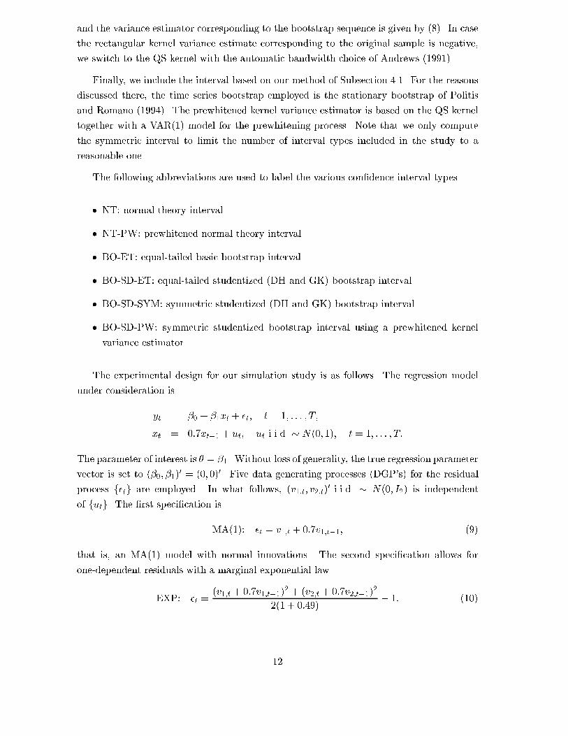
and the variance estimator corresponding to the bootstrap sequence is given by (8). In case
the rectangular kernel variance estimate corresponding to the original sample is negative,
we switch to the QS kernel with the automatic bandwidth choice of Andrews (1991).
Finally, we include the interval based on our method of Subsection 4.1. For the reasons
discussed there, the time series bootstrap employed is the stationary bootstrap of Politis
and Romano (1994). The prewhitened kernel variance estimator is based on the QS kernel
together with a VAR(1) model for the prewhitening process. Note that we only compute
the symmetric interval to limit the number of interval types included in the study to a
reasonable one.
The following abbreviations are used to label the various con�dence interval types.
� NT: normal theory interval
� NT-PW: prewhitened normal theory interval
� BO-ET: equal-tailed basic bootstrap interval
� BO-SD-ET: equal-tailed studentized (DH and GK) bootstrap interval
� BO-SD-SYM: symmetric studentized (DH and GK) bootstrap interval
� BO-SD-PW: symmetric studentized bootstrap interval using a prewhitened kernel
variance estimator
The experimental design for our simulation study is as follows. The regression model
under consideration is
yt = �0 + �1xt + �t; t = 1; : : : ; T;
xt = 0:7xt�1 + ut; ut i.i.d � N(0; 1); t = 1; : : : ; T:
The parameter of interest is � = �1. Without loss of generality, the true regression parameter
vector is set to (�0; �1)0 = (0; 0)0. Five data generating processes (DGP's) for the residual
process f�tg are employed. In what follows, (v1;t; v2;t)0 i.i.d. � N(0; I2) is independent
of futg. The �rst speci�cation is
MA(1): �t = v1;t + 0:7v1;t�1; (9)
that is, an MA(1) model with normal innovations. The second speci�cation allows for
one-dependent residuals with a marginal exponential law
EXP: �t =(v1;t + 0:7v1;t�1)
2 + (v2;t + 0:7v2;t�1)2
2(1 + 0:49)� 1: (10)
12

The third speci�cation considered is a Markov regime-switching model (Hamilton, 1989).
Here, dt is an unobserved state variable which takes on the values 0 or 1 with Markovian
transition probabilities
Prob (dt = 1jdt�1 = 1) = 0:9; P rob (dt = 0jdt�1 = 1) = 0:1
Prob (dt = 1jdt�1 = 0) = 0:25; P rob (dt = 0jdt�1 = 0) = 0:75:
Then, the residual process is de�ned by
MARKOV: �t = 0:25v1;t + dt �E(�t): (11)
The fourth speci�cation is an AR(1) model with normal innovations
AR(1): �t = 0:7�t�1 + v1;t: (12)
A variation, yielding conditionally heteroskedastic residuals, is the last speci�cation
AR(1)-HET: ~�t = 0:7~�t�1 + v1;t; �t = jxtj~�t: (13)
As in Andrews (1991), the computational burden is reduced by transforming both
(y1; : : : ; yT ) and (x1; : : : ; xT ) to mean zero vectors before running the regression; the same is
done to the bootstrap samples. Note that, after the transformation, we are left with a uni-
variate regressor, which much simpli�es the computations. The transformation is close to
the identity transformation with a high probability and should a�ect the simulation results
very little. We also ran some `untransformed' simulations for several scenarios to check this
intuition and the results were identical up to simulation error.
Sample sizes included are T = 50, T = 100, and T = 200. Block sizes for the bootstrap
methods are b = 3 and b = 5 when T = 50 and b = 5 and b = 10 when T = 100 or
T = 200, respectively. The number of bootstrap replications is K = 1; 000. Estimated
coverage probabilities are based on 1,000 replications per scenario, with all interval types
being computed on the same replications. Note that the accuracy of these estimates was
improved by the use of the control variate technique (Davidson and MacKinnon, 1981). To
this end, for each scenario the true �nite sampling distribution of the OLS estimator �1 was
approximated from 50,000 replications.
Remark 5.1 It would have been interesting to include an automatic choice of the block
size like Algorithm 4.1 into the simulation study. Unfortunately, this was not possible. Even
with the two �xed block sizes, each of Tables 1{5 represents roughly a full day of computing
time using stand-alone C++ code on a supercomputer HP-Convex Exemplar SPP S2000.
Keep in mind that the algorithm to determine the block size is computationally more
demanding by an order of magnitude, so a corresponding table would take several months!
The results are listed in tables Tables 1{ 5. The �ndings can be summarized as follows.
13
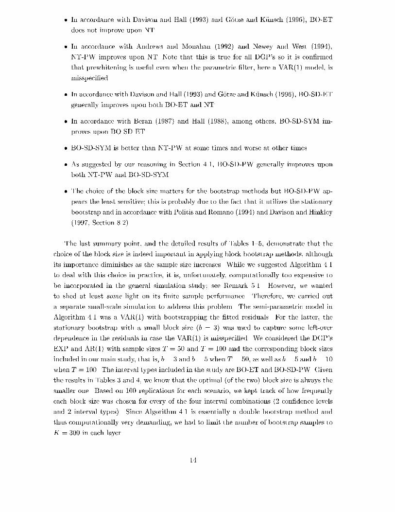
� In accordance with Davison and Hall (1993) and G�otze and K�unsch (1996), BO-ET
does not improve upon NT.
� In accordance with Andrews and Monahan (1992) and Newey and West (1994),
NT-PW improves upon NT. Note that this is true for all DGP's so it is con�rmed
that prewhitening is useful even when the parametric �lter, here a VAR(1) model, is
misspeci�ed.
� In accordance with Davison and Hall (1993) and G�otze and K�unsch (1996), BO-SD-ET
generally improves upon both BO-ET and NT.
� In accordance with Beran (1987) and Hall (1988), among others, BO-SD-SYM im-
proves upon BO-SD-ET.
� BO-SD-SYM is better than NT-PW at some times and worse at other times.
� As suggested by our reasoning in Section 4.1, BO-SD-PW generally improves upon
both NT-PW and BO-SD-SYM.
� The choice of the block size matters for the bootstrap methods but BO-SD-PW ap-
pears the least sensitive; this is probably due to the fact that it utilizes the stationary
bootstrap and in accordance with Politis and Romano (1994) and Davison and Hinkley
(1997, Section 8.2).
The last summary point, and the detailed results of Tables 1{5, demonstrate that the
choice of the block size is indeed important in applying block bootstrap methods, although
its importance diminishes as the sample size increases. While we suggested Algorithm 4.1
to deal with this choice in practice, it is, unfortunately, computationally too expensive to
be incorporated in the general simulation study; see Remark 5.1. However, we wanted
to shed at least some light on its �nite sample performance. Therefore, we carried out
a separate small-scale simulation to address this problem. The semi-parametric model in
Algorithm 4.1 was a VAR(1) with bootstrapping the �tted residuals. For the latter, the
stationary bootstrap with a small block size (b = 3) was used to capture some left-over
dependence in the residuals in case the VAR(1) is misspeci�ed. We considered the DGP's
EXP and AR(1) with sample sizes T = 50 and T = 100 and the corresponding block sizes
included in our main study, that is, b = 3 and b = 5 when T = 50, as well as b = 5 and b = 10
when T = 100. The interval types included in the study are BO-ET and BO-SD-PW. Given
the results in Tables 3 and 4, we know that the optimal (of the two) block size is always the
smaller one. Based on 100 replications for each scenario, we kept track of how frequently
each block size was chosen for every of the four interval combinations (2 con�dence levels
and 2 interval types). Since Algorithm 4.1 is essentially a double bootstrap method and
thus computationally very demanding, we had to limit the number of bootstrap samples to
K = 300 in each layer.
14
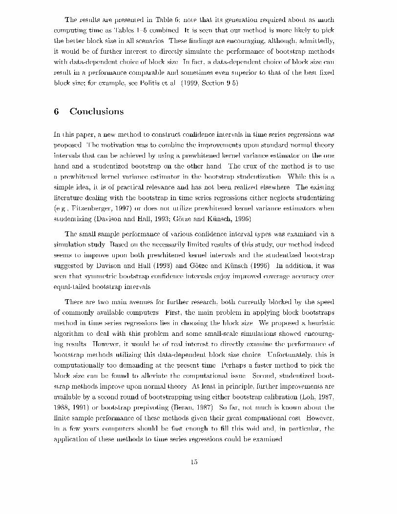
The results are presented in Table 6; note that its generation required about as much
computing time as Tables 1{5 combined. It is seen that our method is more likely to pick
the better block size in all scenarios. These �ndings are encouraging, although, admittedly,
it would be of further interest to directly simulate the performance of bootstrap methods
with data-dependent choice of block size. In fact, a data-dependent choice of block size can
result in a performance comparable and sometimes even superior to that of the best �xed
block size; for example, see Politis et al. (1999, Section 9.5).
6 Conclusions
In this paper, a new method to construct con�dence intervals in time series regressions was
proposed. The motivation was to combine the improvements upon standard normal theory
intervals that can be achieved by using a prewhitened kernel variance estimator on the one
hand and a studentized bootstrap on the other hand. The crux of the method is to use
a prewhitened kernel variance estimator in the bootstrap studentization. While this is a
simple idea, it is of practical relevance and has not been realized elsewhere. The existing
literature dealing with the bootstrap in time series regressions either neglects studentizing
(e.g., Fitzenberger, 1997) or does not utilize prewhitened kernel variance estimators when
studentizing (Davison and Hall, 1993; G�otze and K�unsch, 1996).
The small sample performance of various con�dence interval types was examined via a
simulation study. Based on the necessarily limited results of this study, our method indeed
seems to improve upon both prewhitened kernel intervals and the studentized bootstrap
suggested by Davison and Hall (1993) and G�otze and K�unsch (1996). In addition, it was
seen that symmetric bootstrap con�dence intervals enjoy improved coverage accuracy over
equal-tailed bootstrap intervals.
There are two main avenues for further research, both currently blocked by the speed
of commonly available computers. First, the main problem in applying block bootstraps
method in time series regressions lies in choosing the block size. We proposed a heuristic
algorithm to deal with this problem and some small-scale simulations showed encourag-
ing results. However, it would be of real interest to directly examine the performance of
bootstrap methods utilizing this data-dependent block size choice. Unfortunately, this is
computationally too demanding at the present time. Perhaps a faster method to pick the
block size can be found to alleviate the computational issue. Second, studentized boot-
strap methods improve upon normal theory. At least in principle, further improvements are
available by a second round of bootstrapping using either bootstrap calibration (Loh, 1987,
1988, 1991) or bootstrap prepivoting (Beran, 1987). So far, not much is known about the
�nite sample performance of these methods given their great compuational cost. However,
in a few years computers should be fast enough to �ll this void and, in particular, the
application of these methods to time series regressions could be examined.
15

References
Andrews, D.W.K. (1991). Heteroskedasticity and autocorrelation consistent covariance ma-
trix estimation. Econometrica 59, 817{858.
Andrews, D.W.K. and Monahan, J.C. (1992). An improved heteroskedasticity and autocor-
relation consistent covariance matrix estimator. Econometrica 60, 953{966.
Beran, R. (1987). Prepivoting to reduce level error of con�dence sets. Biometrika 74, 457{68.
Davidson, R. and MacKinnon, J.G. (1981). E�cient estimation of tail-area probabilities in
sampling experiments. Economic Letters 8, 73{77.
Davison, A.C and Hall, P. (1993). On studentizing and blocking methods for implementing
the bootstrap with dependent data. Australian Journal of Statistics 35, 215{224.
Davison, A.C. and Hinkley, D.V. (1997). Bootstrap Methods and their Application. Cam-
bridge University Press.
Fitzenberger, B. (1997). The moving blocks bootstrap and robust inference for linear least
squares and quantile regressions. Journal of Econometrics 82, 235{287.
G�otze, F. and K�unsch, H.R. (1996). Second order correctness of the blockwise bootstrap
for stationary observations. Annals of Statistics 24, 1914{1933.
Hall, P. (1988). On symmetric bootstrap con�dence intervals. Journal of the Royal Statistical
Society, Ser. B 50, 35{45.
Hall, P. (1992). The Bootstrap and Edgeworth Expansion. Springer, New York.
Hall, P., Horowitz J.L., and Jing, B.-Y. (1996). On blocking rules for the bootstrap with
dependent data. Biometrika 50, 561{574.
Hamilton, J.D. (1989). A new approach to the economic analysis of nonstationary time
series and the business cycle. Econometrica 57, 357{384.
Hannan, E.J. (1970). Multiple Time Series. John Wiley, New York.
K�unsch, H.R. (1989). The jackknife and the bootstrap for general stationary observations.
Annals of Statistics 17, 1217{1241.
Liu, R.Y. and Singh, K. (1992). Moving blocks jackknife and bootstrap capture weak depen-
dence. In Exploring the Limits of Bootstrap, 225{248. Edited by LePage, R. and Billard,
L., John Wiley, New York.
Loh, W.Y. (1987). Calibrating con�dence coe�cients. Journal of the American Statistical
Association 82, 155{162.
16

Loh, W.Y. (1988). Discussion of \Theoretical comparison of bootstrap con�dence intervals"
by P. Hall. Annals of Statistics 16, 972{976.
Loh, W.Y. (1991). Bootstrap calibration for con�dence interval construction and selection.
Statistica Sinica 1, 479{495.
Newey, W.K. and West, K.D. (1994). Automatic lag selection in covariance matrix estima-
tion. Review of Economic Studies 61, 631{653.
Politis, D.N. and Romano, J.P. (1994). The stationary bootstrap. Journal of the American
Statistical Association 89, 1303{1313.
Politis, D.N. Romano, J.P., and Wolf, M. (1999). Subsampling. Springer, New York.
Press, H. and Tukey, J. W. (1956). Power spectral methods of analysis and their application
to problems in airplane dynamics. Bell Systems Monograph No. 2606.
Priestley, M.B. (1981). Spectral Analysis and Time Series. Academic Press, New York.
White, H. (1984). Asymptotic Theory for Econometricians. Academic Press, Orlando.
Wu, C.F. (1986). Jackknife, bootstrap and other resampling methods in regression analysis.
Annals of Statistics 14, 1261{1343.
17

7 Tables
Table 1: Estimated coverage probabilities (EC) of various con�dence intervals with nominal
levels 0.95 and 0.90. The speci�cation for the residual process is model (9). The �rst two
columns correspond to the smaller block size always.
MA(1) residuals, n = 50, b = 3, and b = 5
Interval EC-0.95 EC-0.90 EC-0.95 EC-0.90
NT 0.87 0.81 0.87 0.81
NT-PW 0.91 0.86 0.91 0.86
BO-ET 0.87 0.80 0.87 0.82
BO-SD-ET 0.92 0.85 0.90 0.83
BO-SD-SYM 0.92 0.86 0.91 0.85
BO-SD-PW 0.93 0.88 0.93 0.88
MA(1) residuals, n = 100, b = 5 and b = 10
Interval EC-0.95 EC-0.90 EC-0.95 EC-0.90
NT 0.91 0.85 0.91 0.85
NT-PW 0.94 0.90 0.94 0.90
BO-ET 0.88 0.82 0.87 0.81
BO-SD-ET 0.91 0.86 0.90 0.85
BO-SD-SYM 0.92 0.87 0.90 0.85
BO-SD-PW 0.95 0.90 0.93 0.88
MA(1) residuals, n = 200, b = 5 and b = 10
Interval EC-0.95 EC-0.90 EC-0.95 EC-0.90
NT 0.92 0.87 0.92 0.87
NT-PW 0.97 0.93 0.97 0.93
BO-ET 0.92 0.87 0.90 0.86
BO-SD-ET 0.94 0.89 0.92 0.87
BO-SD-SYM 0.94 0.89 0.92 0.87
BO-SD-PW 0.95 0.91 0.94 0.89
18

Table 2: Estimated coverage probabilities (EC) of various con�dence intervals with nominal
levels 0.95 and 0.90. The speci�cation for the residual process is model (10). The �rst two
columns correspond to the smaller block size always.
EXP residuals, n = 50, b = 3, and b = 5
Interval EC-0.95 EC-0.90 EC-0.95 EC-0.90
NT 0.91 0.85 0.91 0.85
NT-PW 0.92 0.86 0.92 0.86
BO-ET 0.93 0.87 0.91 0.85
BO-SD-ET 0.91 0.85 0.90 0.84
BO-SD-SYM 0.93 0.87 0.92 0.86
BO-SD-PW 0.94 0.90 0.94 0.89
EXP residuals, n = 100, b = 5 and b = 10
Interval EC-0.95 EC-0.90 EC-0.95 EC-0.90
NT 0.92 0.86 0.92 0.86
NT-PW 0.94 0.88 0.94 0.88
BO-ET 0.93 0.86 0.90 0.85
BO-SD-ET 0.91 0.86 0.89 0.83
BO-SD-SYM 0.93 0.88 0.91 0.86
BO-SD-PW 0.95 0.89 0.93 0.87
EXP residuals, n = 200, b = 5 and b = 10
Interval EC-0.95 EC-0.90 EC-0.95 EC-0.90
NT 0.94 0.88 0.94 0.88
NT-PW 0.95 0.90 0.95 0.90
BO-ET 0.94 0.88 0.94 0.88
BO-SD-ET 0.92 0.85 0.93 0.87
BO-SD-SYM 0.95 0.89 0.94 0.90
BO-SD-PW 0.95 0.90 0.95 0.90
19

Table 3: Estimated coverage probabilities (EC) of various con�dence intervals with nominal
levels 0.95 and 0.90. The speci�cation for the residual process is model (11). The �rst two
columns correspond to the smaller block size always.
MARKOV residuals, n = 50, b = 3, and b = 5
Interval EC-0.95 EC-0.90 EC-0.95 EC-0.90
NT 0.85 0.79 0.85 0.79
NT-PW 0.87 0.82 0.87 0.82
BO-ET 0.86 0.80 0.83 0.77
BO-SD-ET 0.92 0.86 0.90 0.83
BO-SD-SYM 0.93 0.88 0.90 0.84
BO-SD-PW 0.93 0.87 0.92 0.86
MARKOV residuals, n = 100, b = 5 and b = 10
Interval EC-0.95 EC-0.90 EC-0.95 EC-0.90
NT 0.89 0.82 0.89 0.82
NT-PW 0.91 0.85 0.91 0.85
BO-ET 0.88 0.81 0.88 0.80
BO-SD-ET 0.93 0.87 0.90 0.84
BO-SD-SYM 0.94 0.87 0.91 0.85
BO-SD-PW 0.94 0.88 0.92 0.86
MARKOV residuals, n = 200, b = 5 and b = 10
Interval EC-0.95 EC-0.90 EC-0.95 EC-0.90
NT 0.90 0.82 0.90 0.82
NT-PW 0.92 0.87 0.92 0.87
BO-ET 0.88 0.81 0.90 0.84
BO-SD-ET 0.92 0.86 0.93 0.87
BO-SD-SYM 0.92 0.87 0.93 0.88
BO-SD-PW 0.93 0.88 0.94 0.90
20
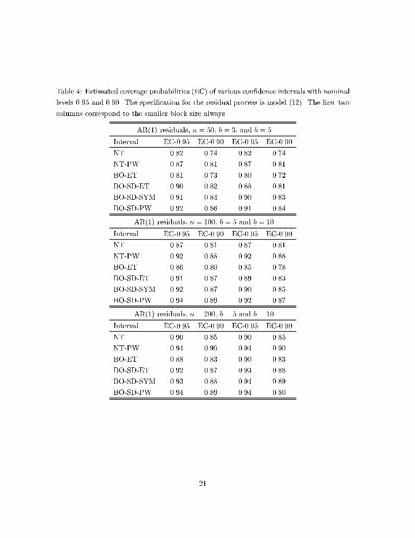
Table 4: Estimated coverage probabilities (EC) of various con�dence intervals with nominal
levels 0.95 and 0.90. The speci�cation for the residual process is model (12). The �rst two
columns correspond to the smaller block size always.
AR(1) residuals, n = 50, b = 3, and b = 5
Interval EC-0.95 EC-0.90 EC-0.95 EC-0.90
NT 0.82 0.74 0.82 0.74
NT-PW 0.87 0.81 0.87 0.81
BO-ET 0.81 0.73 0.80 0.72
BO-SD-ET 0.90 0.82 0.88 0.81
BO-SD-SYM 0.91 0.84 0.90 0.83
BO-SD-PW 0.92 0.86 0.91 0.84
AR(1) residuals, n = 100, b = 5 and b = 10
Interval EC-0.95 EC-0.90 EC-0.95 EC-0.90
NT 0.87 0.81 0.87 0.81
NT-PW 0.92 0.88 0.92 0.88
BO-ET 0.86 0.80 0.85 0.78
BO-SD-ET 0.91 0.87 0.89 0.83
BO-SD-SYM 0.92 0.87 0.90 0.85
BO-SD-PW 0.94 0.89 0.92 0.87
AR(1) residuals, n = 200, b = 5 and b = 10
Interval EC-0.95 EC-0.90 EC-0.95 EC-0.90
NT 0.90 0.85 0.90 0.85
NT-PW 0.94 0.90 0.94 0.90
BO-ET 0.88 0.83 0.90 0.83
BO-SD-ET 0.92 0.87 0.93 0.88
BO-SD-SYM 0.93 0.88 0.94 0.89
BO-SD-PW 0.94 0.89 0.94 0.80
21

Table 5: Estimated coverage probabilities (EC) of various con�dence intervals with nominal
levels 0.95 and 0.90. The speci�cation for the residual process is model (13). The �rst two
columns correspond to the smaller block size always.
AR(1)-HET residuals, n = 50, b = 3, and b = 5
Interval EC-0.95 EC-0.90 EC-0.95 EC-0.90
NT 0.79 0.70 0.79 0.70
NT-PW 0.84 0.76 0.84 0.76
BO-ET 0.75 0.67 0.74 0.67
BO-SD-ET 0.89 0.82 0.88 0.81
BO-SD-SYM 0.92 0.85 0.91 0.85
BO-SD-PW 0.92 0.86 0.92 0.85
AR(1)-HET residuals, n = 100, b = 5 and b = 10
Interval EC-0.95 EC-0.90 EC-0.95 EC-0.90
NT 0.86 0.78 0.86 0.78
NT-PW 0.91 0.85 0.91 0.85
BO-ET 0.82 0.76 0.81 0.73
BO-SD-ET 0.91 0.85 0.90 0.83
BO-SD-SYM 0.93 0.88 0.92 0.86
BO-SD-PW 0.94 0.90 0.93 0.88
AR(1)-HET residuals, n = 200, b = 5 and b = 10
Interval EC-0.95 EC-0.90 EC-0.95 EC-0.90
NT 0.89 0.82 0.89 0.82
NT-PW 0.93 0.88 0.93 0.88
BO-ET 0.86 0.79 0.89 0.82
BO-SD-ET 0.91 0.86 0.92 0.87
BO-SD-SYM 0.93 0.88 0.94 0.89
BO-SD-PW 0.94 0.90 0.95 0.90
22
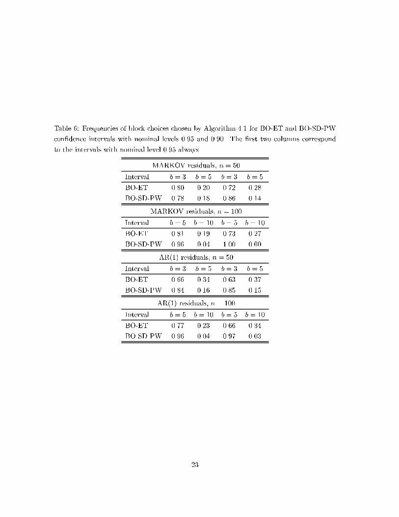
Table 6: Frequencies of block choices chosen by Algorithm 4.1 for BO-ET and BO-SD-PW
con�dence intervals with nominal levels 0.95 and 0.90. The �rst two columns correspond
to the intervals with nominal level 0.95 always.
MARKOV residuals, n = 50
Interval b = 3 b = 5 b = 3 b = 5
BO-ET 0.80 0.20 0.72 0.28
BO-SD-PW 0.78 0.18 0.86 0.14
MARKOV residuals, n = 100
Interval b = 5 b = 10 b = 5 b = 10
BO-ET 0.81 0.19 0.73 0.27
BO-SD-PW 0.96 0.04 1.00 0.00
AR(1) residuals, n = 50
Interval b = 3 b = 5 b = 3 b = 5
BO-ET 0.66 0.34 0.63 0.37
BO-SD-PW 0.84 0.16 0.85 0.15
AR(1) residuals, n = 100
Interval b = 5 b = 10 b = 5 b = 10
BO-ET 0.77 0.23 0.66 0.34
BO-SD-PW 0.96 0.04 0.97 0.03
23