Working for the Future: Female Factory Work and ChildHealth in Mexico∗

David Atkin†

May 2011Extremely preliminary and incomplete, please do not cite.

Abstract

In this paper, I show that in Mexico the height of children is significantly higher for cohorts

of women who were heavily exposed to new factory opening as young women. The effects are

concentrated on female children, and correspond to an increase in female child height-for-age

Z scores of 0.2 standard deviations for cohorts who experienced the largest female employ-

ment shocks (a shock at the 95th percentile). If these cohort-level impacts operate exclusively

through changing the probability of factory employment for women, I obtain estimates of the

impact of factory work on child height through an IV strategy that are an order of magnitude

larger than the cohort effects above. These magnitudes are implausibly large unless the local

average treatment effect group is comprised of women with unusually large benefits from fac-

tory work and so select into manufacturing precisely for that reason. Therefore, the results are

suggestive that the child health impacts of new factory openings spread beyond simply the set

of mothers induced to enter factory employment.

∗Special thanks to David Kaplan at ITAM for computing and making available the IMSS Municipality level em-ployment data. Further thanks to Angus Deaton, Marco Gonzalez-Navarro, Amit Khandelwal, Fabian Lange, AdrianaLleras-Muney, Nancy Qian and the participants of the Public Finance Workshop at Princeton University for their usefulcomments. Any errors contained in the paper are my own.†Yale University Department of Economics, BREAD, CEPR and NBER. E-mail: david.atkin@yale.edu

1 Introduction

The last half century saw an enormous expansion in both female labor force participation andlow-skill manufacturing around the developing world (Mammen and Paxson 2000). Industrializa-tion may have been expected to increase labor demand primarily for men, who through a combi-nation of cultural and physical reasons were initially favored in industrial jobs in most developingcountries (Goldin 1994). However, in the developing world one of the most publicized aspects ofindustrialization has been the extensive employment of young women in low-skilled manufactur-ing, from the sweat shops of South East Asia, to the Maquiladoras of Mexico.

Many commentators, both inside and outside academia, have linked the globalization of pro-duction to an increase in demand for low-wage female workers in manufacturing. Export-orientedmanufacturing industries such as textiles and low-skilled assembly work often have a preferencefor female labor. The explanations for this preference for female workers include women havinggreater agility, a higher tolerance for repetitive tasks, lower wages and being more docile and lesslikely to unionize (Standing 1999, Fontana 2003, Fernández-Kelly 1983).

Whilst there is much speculation on the effects of female factory employment, there is very lit-tle rigorous evaluation. Increasing female factory employment opportunities would be expected toincrease female incomes, at least for the women who obtain such jobs. In societies in which womanare traditionally confined to work in the home or on the family farm, rising extra-household em-ployment opportunities may have transformative effects on female empowerment and a woman’sability to make her own life choices, especially regarding marriage, fertility and household spend-ing.

Much of the academic work that explores the impacts of female factory employment focuseson Bangladesh, where textile exports make up about 80% of total merchandise exports and theseindustries primarily employ young rural women who have very few other extra-household em-ployment opportunities. Kabeer (2002), Kabeer (1997), and Hewett and Amin (2000) provideevidence that working in a textiles factory is associated with higher female status, stronger intra-household bargaining power and better quality of life measures. In contrast, human rights groupsand anti-sweatshop activists often focus on the negative effects of female factory work; arduous,exploitative and unsafe working conditions, verbal and physical abuse at the workplace alongsidesocial ostracization outside it.

In this paper, I explore one particular impact of female factory work that has not yet receivedattention in the literature. I estimate the impact of the expansion of factory employment opportu-nities for young women in Mexico on the later health of their children. A priori, the effects areambiguous. Although the expansion in female employment opportunities are likely to raise house-hold incomes though employment and wage effects, there are a myriad of other possible routes

2

that have more ambiguous effects on child health. As in the Bangladesh context, intra-householdbargaining power may change and the perceived returns to child health may be altered, particularlyfor girls. Both of these channels would tend to lead to improved child health. In contrast, fe-male factory work may lead to changes that are detrimental to child health: lower maternal health,lower quality husband matches or less time at home caring for children. Finally, new factory em-ployment opportunities may induce school dropout and hence also lower education and long runincome earning potential, as shown by Atkin (2009).

The basic difficulty in determining the causal effects of expansions in female manufacturingopportunities on child health comes from the fact that where factories locate and the women whochoose to work in them are highly selected. Factories locate in particular areas of the country,drawn by worker characteristics and local wage rates, or fixed geographic features (e.g. beingclose to the US border). The women who work in the factories are often from poorer segments ofsociety, but also perhaps highly driven and willing to buck societal norms.

In this paper, I exploit the enormous regional and temporal variation in new factory openingsthat occurred in Mexico between 1986 and 2000. Over this time period, Mexico saw a huge surgein female manufacturing employment, closely associated with the growth in textiles and exportassembly operations that followed trade liberalization. I use the differential timing of new factoryopportunities across cohorts within municipalities to plausibly identify the cohort level effects oflarge female factory employment expansions on the women reaching adulthood at the time.1

___________________________Discuss results here [INCOMPLETE]____________________________________There is a large literature detailing how female income and employment options affect house-

hold decision making by changing the bargaining power within a marriage. Strauss and Thomas(1995) and Behrman (1997) provide extensive surveys of this literature. Many papers find thatwomen have stronger relative preference for expenditures on child goods than men do, and accord-ingly, increasing female income increases child education and health outcomes (Thomas 1997).Additionally, women may have a relatively stronger preference than men for expenditures on fe-male children (Duflo 2003). More directly, Qian (2008) shows that female child survival ratesrose with greater income earning opportunities for women in China. This paper is also closelyrelated to a recent literature that finds increases in female education associated with the growthof female labor market opportunities in the service sector in India (Jensen 2009, Munshi andRosenzweig 2006, Oster 2010).

1I focus on employment shocks at age 16, when a woman is legally allowed to b employed in formal manufac-turing, and compulsory education should be completed. I argue that the detrended year to year variation in the arrivalof new factory opportunities is plausibly exogenous to female characteristics that may affect child health investmentsdirectly.

3

This literature together the limited work on female factory employment suggests that femalefactory work may affect child outcomes through higher female incomes. Female manufacturingjobs may also lead to a more general increase in female empowerment if these jobs provide oneof the few opportunities for women to work outside of the household in a formal employmentenvironment. Surprisingly, no work has assessed these effects directly. Given the importanceof early life health and education investments on later life outcomes for a child, the impact offemale factory work on these investments is a vital component in assessing the welfare impact ofexpansions in female manufacturing employment in developing countries.

___________________________Outline sections here [INCOMPLETE]____________________________________

2 Background on Mexico’s Industrialization 1985-2000

Mexico provides a perfect setting to study the impacts of globalization and the expansion offemale manufacturing opportunities on the young women whose lives are changed by these events.In this paper, I will investigate one particular dimension, the child health decisions made by thesecohorts of women. To identify such effects, I will exploit the enormous regional and temporalvariation in the arrival of a large number of new female manufacturing opportunities.

Over the period spanned by the data (1985-2000), Mexico turned its back on an import substitu-tion strategy and liberalized trade, joining GATT in 1986 and NAFTA in 1994. During these years,Mexico reduced tariffs substantially and many new plants opened, often in the form of Maquilado-ras, to manufacture products for export.2 These firms were initially confined to border areas, butby the year 2000 one quarter of firms were in non-border states. Total employment in formal sectormanufacturing rose from 1.6 million jobs at the beginning of 1986 to over 4.2 million jobs in 2000.The major export sectors of textiles and apparel, electrical assembly and transportation equipmentaccounted for much of this, with employment rising from under 900,000 formal sector jobs at thebeginning of 1986 to over 2.7 million jobs in 2000. Much of this growth was driven by multi-national corporations, with nearly two thirds of manufacturing exports in 2000 originating fromforeign affiliates (UNCTAD 2002).

Unlike the manufacturing plants that existed prior to this period in Mexico, women constitutedthe majority of employees in many of these new export operations. The explanations for this pref-erence for female workers include women having greater agility, a higher tolerance for repetitivetasks, lower wages and being more docile and less likely to unionize (Standing 1999, Fontana

2The Maquiladora program allows duty free imports of goods for assembly and re-export.

4

2003, Fernández-Kelly 1983). For example, 77 percent of blue-collar workers in Maquiladoraswere female in 1980, although this number fell to 55 percent by 2000.

Coincident with the expansion of female manufacturing opportunities, Female labor force par-ticipation rose from 28% of the total labor force in 1985 to 40% in 2000 (Moreno-Fontes Chammartin2004), with a particularly pronounced increase in the manufacturing sector. More precisely, in1985 there were 341,105 women in registered private manufacturing and this rose to 1,493,736women by 2000, with those employed in export sectors rising from 200,635 to 966,722 women.3

While there was population growth over the period, it was at a much slower rate. The 1990 Mexi-can census recorded 21 million females aged 15-49, rising to 26 million in 2000. Accordingly theproportion of the formal sector manufacturing employees that were female rose from 21.7 percentin 1986 to 34.7 percent in 2000.

3 Data

The data used in this paper come from two sources. All the individual level data come from the2002 baseline round of the Mexican Family Life Survey (MxFLS). This survey is a very extensivepanel study of 8,800 households collected by the Centro de Investigacion y Docencia Economicasand the Universidad Iberoamericana, and representative at the national level. There were 38,000individual interviews conducted covering income, employment, consumption, health, access toservices, anthropometrics, education and many other categories. For further details see Rubalcavaand Teruel (2007) The data are particular suited to this study as they ask fairly detailed questionson employment history including the sector and timing of an individuals first job as well as theircurrent job. This allows me to look at the effects of factory employment for women on outcomesthat are only observable later in their life. Detailed anthropometric data was collected providinggood measures of child health. Finally, all of these individuals can be matched to their currentmunicipality, and migration histories are recorded.

The second data source is the Mexican Social Security Institute (IMSS), which has employmentinformation on the complete universe of formal private sector establishments. This data come fromthe social security system into which all formal employees are required to enroll. The data are heldsecurely at ITAM where the aggregations from firm to municipality level were carried out. I usethe total employment data broken down by sex for a variety of industries at the municipality level.The data cover 1985 to 2000 and is the total number of employees on December 31st of that year.Kaplan, Gonzalez, and Robertson (2007) contains further details.

3Authors calculation based on data from Mexican Social Security Institute (IMSS) which contains the completeuniverse of registered private firms. Export sectors are two digit industries where over half the output was exportedin at least half the years between 1985 and 2000. The export and output data come from the Trade, Production andProtection 1976-2004 database (Nicita and Olarreaga 2007).

5

The two data sets are combined leaving 112 municipalities where MxFLS data was collectedand IMSS data on employment opportunities are available. There are 136 municipalities in theMxFLS. As I will be using the IMSS data to create a measure of local labor market employmentopportunities, some of these municipalities a located next to each other and should be treated asa single labor market. Therefore, I merge municipalities to correspond to metropolitan zones asdefined by INEGI.4 The INEGI metropolitan zones correspond closely to single labor markets, asthe boundaries of towns are in part determined by commuter data recorded in the 2000 Mexicancensus.

When I restrict the sample to women who filled in the adult survey (women over the age of 15in 2002), just over 9,500 women are in my sample. This sample is further reduced to about 4,215women who entered adulthood during the period 1985-2000 covered by the employment data. Mymain specification focuses on the 3,018 women who lived in their current municipality at age 16,the time of the municipality labor demand shock I study.

3.1 Exploring the Data [INCOMPLETE]

Before tackling the impact of female factory employment opportunities on child investment, Iwill explore the nature of female manufacturing in Mexico using the MxFLS data.

The MxFLS survey provides extensive employment data. Most usefully, the survey asks thesector of the respondents first job, and how old they were. Table 1 shows how various outcomesvary by sector of first employment. I restrict the sample to women who turned 16 between 1986and 2000 and so are aged between 18 and 31 in 2002 as this is the range of years for which I havedata on the employment environment. Finally I restrict the sample to women who were living intheir current municipality at age 16, as ultimately I will be matching employment data to womenat the municipality level, and the MxFLS data does not report the name of their municipality at age16 if it was not the same as their current municipality. All these characteristics are weighted bysurvey weights representative at the national level, except where I report frequencies. I have 3,106women in the sample. 1,433 of these women have children, and there are 3,018 of these children.

Women who first worked in Agriculture, Manufacturing and Personal Services are less edu-cated, start work younger, consume less and have lower household incomes and more childrencompared to other women who have worked. These women who first worked in Agriculture, Man-ufacturing and Personal Services look fairly similar to women who have never worked. Some ofthese effects could be coming from different sectoral growth trends, but in the regressions I includetime controls. The large variation between professions strongly suggests that personal characteris-tics are correlated with initial sectoral choices.

4For a robustness check, I will exclude Mexico City, Monterrey and Guadalajara as these are very large cities andmy survey weighted results may be driven by these 3 metropolitan zones.

6

Table 2 shows where women whose first job was in manufacturing currently work, and forwomen whose current job is in manufacturing, where their first job was. Not working, retail,food and transport and to a lesser degree personal services seem to be the main alternatives tomanufacturing work for these women. Having a first job in manufacturing for most women seemsto mean they are either still working in manufacturing or have left the labor force (78% of them).

So far very little has been said about migration. Columns 6 and 7 of table 1 compares thesample of women who were living in their current municipality at age 16 with those who werenot. Only about 70% of the women are living in the same municipality as they were living in atage 16. As ultimately I will be matching employment data to women at the municipality level, andthe MxFLS data does not report the name of their origin municipality, it is important to see howdifferent these non-migrants are. Migrants seem to be slightly wealthier and more educated. Thepolicy maker (especially if they are a local politician) may be more concerned about the effect ofmanufacturing on the children of current residents than the children of the women who migrateto the town if a factory opens. Therefore, omitting migrants may provide the correct parameterof interest for a local industrial policymaker. However, as I can only pick up the effects on thepopulation that decided not to migrate, this is not the complete picture.

It is possible to get an idea of the comparative earnings in these sectors from current employ-ment data . Table 3 shows the earnings in pesos both for the last month and the last year brokendown by sector of employment. Manufacturing income is relatively high, larger than incomesof women in the Retail, Food and Transport sector whose employees are better educated. Thehourly wage is relatively lower as manufacturing has long hours. However, at least the medianhourly manufacturing wage (which will be a more reliable indicator in the presence of outliers) isstill higher than agriculture, retail and personal services. Certainly, it seems believable that thesemanufacturing jobs are relatively good jobs for low-skilled women.

Finally, table4 reports the means of the various health measures and mother employment shocksfor the children in my sample.

___________________________Discuss child measures and employment shock distribution here [INCOMPLETE]____________________________________

4 Reduced Form Evidence

The basic question I will try to address is what are the health impacts of large expansions in fe-male factory opportunities for the children of the women who reached adulthood during this period.In a related paper, Atkin (2009), I explore the educational responses to new factory employmentopportunities in Mexico. In that paper, I match cohort education levels with local manufacturing

7

employment shocks at key school leaving ages and find that cohort education levels were lowerwhen there were large expansions in export manufacturing opportunities around age 16. I willfollow a very similar empirical strategy in this paper.

In particular, I match women in the 2002 MxFLS cross-section to a measure of the local femalemanufacturing vacancies from the IMSS private formal sector employment rolls. I focus on the thelocal manufacturing opportunities available to the woman in the first year when she should havecompleted her compulsory education requirements and also becomes legally eligible to work inthe formal sector manufacturing sector, age 16.

4.1 Female Sectoral Choice and Large Factory Employment Shocks at Age16

Prior to exploring the effects of these maternal employment shocks on child health, I will justifymy choice of explanatory variable by demonstrating that large expansions in female manufacturingemployment at this age significantly increased the probability that a woman chooses to work in themanufacturing sector. I use the following specification:

Manu ficm = α + β1l50f em,age16,icm + dm + dc + λmagec + εicm. (1)

where i subscripts women, m is the municipality where the mother currently lives. Manu fim is adummy variable that takes the value 1 if a woman worked in manufacturing as her first job. Giventhe lack of a complete job history in the MxFLS, this is the best indicator available of the sectoralchoices women are making as young women. The indicator does however miss women who startworking in manufacturing while young but not as their first job.

My measure of local female manufacturing vacancies, l50f em,age16,icm, are the net new jobs cre-

ated for women by local manufacturing firms in the year that the woman was aged 16 divided bythe working age female population in the municipality. The measure is scaled by total working agefemale population as it is obvious that one factory opening in a city of 500,000 will have a muchsmaller effect on the probability of working in manufacturing than if the same factory opened in atown of 15,000. The working age female population is defined as women aged 15 to 49 from theMexican Census of 1990 and 2000 and the Conteo de Población y Vivienda 1995, with the otheryears interpolated.5

I restrict attention only to large expansions or contractions where 50 or more employees werehired or laid off in a single firm in a single year in a firm classified as manufacturing by IMSS.6

5All this data was obtained from the INEGI website at www.inegi.gob.mx.6The results are robust to lowering the cutoff from 50 to 25.

8

For example in year y, l50f em,age16,ym =

∑manuf firms k∆empmyk1[|∆empmyk|>50]

female working age pop.my. I then construct an

individual l50f em,age16,icm for each woman, taking a weighted average of the values of l50

f em,age16,ym

for the two calendar years in which the woman was aged 16, with weights based on the woman’sexact birthday.

There are two reasons for focusing only on large expansions and contractions. If formal sectorlabor markets clear, a woman with a particularly strong desire to enter manufacturing as soon asshe turns 16 will mechanically raise the number of new jobs created that year. Therefore, estimatedof β̂1 will be potentially endogenous. However, these large firm expansions and contractions aremore plausibly exogenous to the characteristics of individual cohorts, a point I will elaborate onin more detail in section 4.3 when I discuss my main specification where I regress child height onl50

f em,age16,icm. I note at this stage that any individual characteristic that enters in the error term ofequation 1 but does not affect child height will bias β̂1 but will not bias estimates of .

Secondly, many of the mechanisms through which female manufacturing employment oppor-tunities may alter child health are most relevant for factory work. Small home or workshop-basedmanufacturing may be more comparable to previously existing female employment opportunitiesand therefore have less transformative effects. As large employment changes can only occur atlarge factories, my employment shock measure automatically excludes changes in such employ-ment opportunities.

The choice of age 16 is an obvious one as that is the legal age for starting manufacturing workin the formal sector.7 While it is certain that some female employees are younger and have forgeddocuments, Mexican factories do not have a particularly large problem with child labor.8 Age 16is also the age children start upper secondary school and so is a common age to drop out of schooland start work.

Additionally, I include location fixed effects dm (at the municipality level, or metropolitan zoneif a conurbation contains several municipalities), woman’s age fixed effects dc, and linear timetrends in mothers age that are estimated separately for each municipality level λmagec. I includethese trends to control for the fact that if manufacturing was becoming an increasingly commonjob for women in a specific municipality throughout the period, Manu ficm will be correlated withany variable that trends over time in that type of municipality. So most obviously, if fast growingmunicipalities saw new job creation increasing in each year as well as a growing proportion ofwoman working in manufacturing, I would pick up a spurious correlation even if employment

7The minimum working age is 14 in Mexico, but rises to 16 in sectors considered hazardous, which includesmany industrial sectors. Additionally children aged 14 and 15 require parental consent, a document confirming theyare medically fit and can not work overtime or beyond 10pm. Accordingly, the minimum working age in the formalmanufacturing sector is usually stated as 16.

8For example the Congressionally mandated "By the Sweat and Toil of Children" (US Department of Labor 1994)reports that "there is only limited evidence of the existence of child labor in maquilas currently producing goods forexport although there have been past reports of child labor".

9

shocks at age 16 made women no more likely to work in manufacturing.___________________________Discuss results here [INCOMPLETE]The results of regression 1 are shown in table 5. In columns 1 to 4, I restrict my sample of

women to only those “at risk”. My local employment shocks at age 16 should only alter the firstsector of employment of young women who were living in the municipality at the time and had notyet started working at this age, and I define this as the “at risk” group. In column 5 I also includethe women who are not at risk, and interact the job shock with an indicator for whether the womanis not at risk.

• There are significant effects of age 16 new factory hires on the sector of first employment.

• The coefficient size of 6.8 is a reasonable magnitude. If there were 100 new jobs and 100unemployed women all age 16 wishing to enter employment in the town, and no one couldmove jobs, the coefficient should equal 1 if the jobs were suitably attractive. However, theworking age female population picks up a much larger pool of women than those wishingto take a job who have not yet entered the labor force and women who are already workingcan fill the factory jobs, and all women may not want the jobs even if they are available.Therefore, if only one tenth of the working age female population would want such a job,the coefficient would be around 10.

• I include male job arrivals, and reassuringly they do not seem to matter for female employ-ment.

• When I interact new job openings with whether the woman is at risk or not, there are onlyeffects on the “at risk” group of women who were living in the municipality at age 16 andnot already working in manufacturing. This placebo test is evidence that the instrument isindeed picking up new job opportunities that are relevant to women’s employment decisions.

• When I break manufacturing shocks down by sub-sector, sector of first employment in-creases only for the relevant sub-sectors (textiles and apparel, other manufacturing).

• Plot predicted probability of working in manufacturing in figure 1 as well as counterfactualprobability in the absence of any large female employment shocks. Total effect is small, withprobability of employment only going up by about 1.3 percent from 0.057 to 0.070.

• Smaller effects at other ages.

___________________________________________

10

4.2 Child Height and Large Factory Employment Shocks for Mothers

Having established that local factory employment shocks do affect the probabilities of employ-ment in manufacturing, I now explore whether these same shocks affect the children of the heavilyexposed cohorts of women.

The basic specification including controls is:

h f azi jcm = α +β1l50f em,age16,icm +β2l50

f em,age16,icm×Male j+

γMale j +dm +dc +λmagec +dchild age +Xi jcmθ + εi jcm. (2)

where as before i subscripts mothers, m is the municipality where both the child currently livesand the mother lived at age 16, and c is the age cohort of the mother. Additionally, j indexes thechild. The dependent variable is h f azi jcm , the height-for-age Z score of the child. As in regression1, I include the local job shock for the mother at the key school leaving and employment age,municipality and mother age fixed effects, and mother age time trends at the municipality level. Asdiscussed in the introduction, there is a substantial literature on potential gender bias in spendingpatterns and investment decisions in developing countries. Therefore, I allow the health impactsof the factory employment shock to vary by the sex of the child by interacting a dummy variable,Male j, that takes the value of 1 if the child is male.

Child height-for-age Z scores were chosen as my measure of human capital as they are perhapsthe best measure of child health and nutritional status at young ages {citations}. Child height isa cumulative measure of child nutrition and health insults up to that age, and is regularly usedas an indicator of stunting. The impacts of early life nutrition (which height-for-age z scoresare measuring) include earlier mortality, increased morbidity and negative labor market outcomes(Barker 1992, Case, Fertig, and Paxson 2005, Almond 2006, Case and Paxson 2006).

The height-for-age Z scores have been calculated using the WHO child growth standards(WHO Multicentre Growth Reference Study Group 2007). The WHO norms originate from wellnourished children around the world, and so accordingly the averages for my sample are belowzero for both sexes. Female children are on average 0.58 standard deviations below the mean, andmale children are 0.64 standard deviations below the mean.

As a further check I use an additional health metric, weight-for-height Z-scores, which areavailable for the the younger children in my sample.9 A schooling measure would also be desir-able. However, most of the children of these young mothers are either not yet in school, or are atschooling ages where there are only small differences in school attendance across households.

I include three sets of additional control variables, Xi,l . Specification 1 includes no additional

9Weight-for-height Z-score tables are only available for children of age 0-5.

11

controls. This specification will not provide the best estimates of the δ ′s since relevant controls willtend to increase the precision of the estimates. Specification 2 accordingly adds controls that canbe considered characteristics at age 16. These controls are adult height (a good measure of earlierlife nutrition and income) and education capped at grade 9, which most girls should completeby age 15. Events after age 16 can plausibly affect both of these, but they are the observablecharacteristics most likely to be set by that age. These variables could be still be endogenous ifthere are omitted variables correlated both with child investment and mother’s height and educationat age 16. Although I am not directly concerned with the coefficients on the controls, biasedcoefficients may impart a bias on the coefficients of interest, δ1 and δ2, and so it is useful to checkthat these coefficients do not change substantially greatly when the controls are added.

Finally, specification 3 also includes household per capita consumption in 2002 and the numberof siblings. Both of these are plausibly affected by local labor market events at age 16 if they forexample altered a young woman’s sectoral choice. Therefore, this specification is not very usefulfor inference about the magnitude of the effect of working in manufacturing on child health. How-ever, much of their variation in income and fertility will not be related to the sector of employment,and these variables serve as useful controls to show that there is an effect from sectoral choice be-yond that working through income. My preferred specification is accordingly specification 1, butI will refer to specification 2 and 3 where appropriate.

Before reporting the results I will address worries about the identification of the coefficient onβ .

4.3 Identification

In order that the estimated coefficients β̂1 and β̂2 are unbiased and consistent, I require that mymeasure of employment shocks, l50

f em,age16,icm, is exogenous to the error term in equation 2. Myclaim is that the β̂ ’s consistently estimate the effects of new factory openings on child investmentthrough parental channels. Essentially, this claim relies on both the fact that children of samecohort of mothers are born in different years, and that the detrended new factory opening decisionsare uncorrelated with past or future parental factors that affect child health directly.

As I include controls for child age (either age-sex dummies, or age-sex dummies plus municipality-sex fixed effects and municipality-age linear time trends), and effects of new factory openings thatare common across an age cohort of children should be absorbed. For example, a factory may bepolluting, or public expenditures may respond to factory arrivals. I explicitly look for direct effectsof factory opening on children in section 7, and show that these effects are small and insignificant.

It is plausible that a new factory opening in the year that a young woman first decides whetherto enter the labor force will not affect child outcomes directly. The decision of an entrepreneur to

12

open a new factory in a locality will be related to factors such as the local skill distribution, the sizeof the local market and the local infrastructure. For endogenous factory placement to jeopardizethe validity of the instrument, whatever is driving the timing of factory openings within a singlemunicipality (changing population density for example), must also affect child health directly (byaltering public health spending for example). However, many of of these effects would be commonacross all children of the same age group who will have equal exposure to any new facilities, ratherthan common across all children whose mothers are the same age.

The one exception would be variables specific to the cohort of women who are aged 16 at thetime. For example, if women were highly educated for exogenous reasons, this potential laborforce may be attractive to some firms and induce an expansion in female employment creationin manufacturing. Education is likely to also affect child health directly, violating the exclusionrestriction. Similarly, there may be other variables specific to a cohort of women, such as intrinsicdrive, that affect both child health and factory placement. I address this concern in three ways.

First, I exploit the panel dimension of my data. As I have multiple cohorts of women in my dataset, I include municipality fixed effects and linear time trends in mother’s age at the municipalitylevel. This will control for much of the variation in cohort-level variables that would guide firm’slocation decisions. For example, firms being attracted to localities with highly educated womenor rapidly increasing levels of female education. For the exclusion restriction to be violated in thepanel context, a firm must be attracted to a municipality due to deviations in the characteristicsof particular cohorts of women. The error term in the presence of municipality fixed effects isdemeaned by the municipality m average error, εi jcm− ε̄m. As the error term contains future andpast cohort deviations from the trend (divided by the number of time periods), if firms chooseto expand employment in a particular municipality due to on or a few unusual cohorts of youngwomen, the exclusion restriction will be violated. This will be a particular problem if the decisionis based on deviations in the current cohort, as past and future cohort deviations have a muchsmaller effect on the current error term and will become irrelevant as the number of cohorts goesto infinity.

While this violation may be reasonable for small employment changes, for example a smallbusiness expanding employment when it has job applications from impressive female applicants,this is unlikely to be the cause of large factory expansions (or contractions). Therefore, I showresults using only large factory expansions or contractions, where the workforce at a single firmincreased by more than 50 female employees in a single year.

The opening of a new factory is a major investment, with many new employees hired. In acontext such as Mexico, this is likely to be exogenous to deviations in the characteristics of womenin one or two cohorts for several reasons. First, a cohort of women is a very small component ofthe local skill distribution and so will have only a minor influence on the labor pool from which

13

the firm can hire. This assumption is especially plausible for Mexico, which has a large number ofboth informal and migrant workers. Second, entrepreneurs must obtain cohort-varying informationabout the skill level in a municipality, which is not readily available. Instead these large expansionsare most likely driven by external demand factors interacted with stable municipality characteristics(distance to US border, size of local market etc.).

Finally, I can control explicitly for the most obvious characteristics that may drive factorylocation. I can include education obtained prior to the opening of the factory, as well as the heightof women which serves as a crude proxy for health and productivity of the women. In summary,new factory employment opportunities for women in a locality at age 16 are likely to be a validinstrument for whether a woman’s first job was in the manufacturing sector.

4.4 Results

___________________________________________Discuss results here [INCOMPLETE]

• Table 7 shows coefficient of 29.27 on net new manufacturing job arrivals per working agefemale. Find coefficient of -27.67 on interaction with male children. Effect only on girls.

• Do not observe these positive impacts when male jobs arrive (col 3), for the not at risk groupof migrants (column 4), when there is general job growth (col 5) or when female serviecsector jobs arrive (col 6).

• Results robust to inclusion of child-sex trends at municipality level, mother weights, exclud-ing the three largest cities or using fewer controls (Table 9).

• Distribution of shocks shown in figure 2.

• Mean shock leads to child height for age increasing by 0.045 standard deviations for girls(about 0.225 cm for mean age girl of 5).

– 95% shock is about 0.007 net new female jobs per working age female. Impact onfemale child height is about 0.2 standard deviations in this case. About 7% of cohortof women work in factory.

• For 5 year old girl, 1 standard deviation in height-for-age is about 5 cms, for 2 year old it isabout 2.5 cms.

• Compare to Duflo 2003: Pensions received by woman in household increases height for ageof young girls by 1.16 sd, 0.28 (and insignificant) for boys.

___________________________________________

14

5 Causal Pathways

There are multiple pathways through which expansions in female factory labor opportunitieswhen a mother enters adulthood may affect child height. First I will discuss pathways that operatethrough changes in the probability of employment in manufacturing before addressing pathwaysthat may also impact women who don’t end up changing their sectoral employment decisions as aresult of a new factory opening or expansion.

In guiding the discussion, I have a stylized model in mind. I assume that women are forwardlooking and making a joint decision about the sector of initial employment, husband choice andchild health spending, and that the husband and wife may Nash bargain over household spendingdecisions.

Greater female factory labor opportunities increase the probability of employment in manufac-turing. Why might child investment, and particularly female child investment, rise for the womenwho now decide to enter the manufacturing sector for their first job?

First, this labor demand shock will likely lead to higher female incomes at this stage in herlife compared to a woman’s alternative option in the absence of a new factory opening. If childhealth is a normal good, child height would be expected to increase. If female child health is aluxury good, the increase would be larger for girls. Additionally, if a woman is bargaining with herhusband, a higher personal income results in a larger fallback option. Women may have strongerpreferences over child health and particularly female child health, and so child height may increasethrough this channel.

Second, if manufacturing jobs directly raise a woman’s fallback option or bargaining weightin her bargain with her husband, (female) child investment may increase. Manufacturing work ishighly impersonal and almost always done outside of the house in a formal environment. This maydiffer from other common alternatives, where a woman’s income earning ability may be affected byleaving her husband (housework, domestic work for others, small retail). Therefore, manufacturingwork may give a woman a higher payoff if she separates from her husband. Factory experiencemay also give women a greater freedom to migrate, in the expectation that a factory job can beeasily found elsewhere. Similarly, women working in a factory with male supervisors and a non-household environment may develop greater bargaining weight through experiences negotiatingwith men and talking with other women in the factory about their experiences. It is also possiblethat this greater bargaining power is accompanied by a willingness to disobey a husband and makechild investments without his knowledge (e.g. take the child to get a medical checkup withoutdiscussing the decision with her husband), although this does not fit cleanly into a cooperativebargaining model.10

10Note that changes in bargaining weight and the fallback option are clearly differentiable in the context of a Nash

15

Third, manufacturing jobs may change a woman’s expectations about the future earning oppor-tunities for women and hence the perceived returns to human capital investment for her daughter.This will be particularly likely if the alternatives to manufacturing jobs for women are limited toinformal service-sector employment.

Fourth, choosing to take a manufacturing job may alter the woman’s ability to help in the pro-duction of child human capital. For example, if choosing to work in manufacturing is accompaniedby a choice to also obtain less education, a mother may be less able to correctly treat illness, followhealth advice or help with school work. Female manufacturing workers typically work outside thehome. If a woman continues to work in the sector after childbirth, she will be out of the houseduring the work day which may reduce the efficacy of child investment.

Fifth and finally, manufacturing employment may alter a woman’s choice of husband (and sohis characteristics, income and bargaining power) with theoretically ambiguous results. There maybe a stigma attached to female factory work, and so the set of potential husbands may shrink. Atthe same time the woman’s optimization problem will have changed due through the four channelsdetailed above. Therefore, a different husband would be optimally chosen which could eithermagnify or negate the effects above.11

None of these channels are specific to manufacturing. However, for channel 1, the job mustpay high wages compared to the alternative options available. Meanwhile, for channels 2 and 3,the sector must offer a dramatically different employment environment and set of opportunities forwomen compared to traditional jobs. It is also the case that export manufacturing industries areoften the first to successfully break down gender labor norms in traditional societies (Wolf 1992).

I now turn to the women who did not decide to enter manufacturing as a result of the expansionin employment opportunities. For the infra-marginal manufacturing employees, new factory open-ings would have positive wage effects as an increased demand for female manufacturing workerswould raise the female wage in manufacturing. There is abundant evidence that foreign and ex-porting firms in Mexico pay higher wages, and so wage rises from the trade-liberalization inducedfactory expansions may have been substantial.12 New factory openings may have also changedthe type of manufacturing job a woman did. For example, in the absence of a new factory open-ing a woman may have worked in a small manufacturing workshop or even weaving textiles athome. While her first sector of employment is unchanged, a new factory opening may dramati-cally change her work environment as she now decides to work in a large textiles factory. In thisscenario, all the effects listed above for the marginal manufacturing worker may also apply to theinfra-marginal manufacturing workers.

bargain, however empirically they will be impossible to disentangle from each other.11For example, if higher income women are matched with richer husbands, both partners outside options are higher,

and the woman’s bargaining power may not increase.12This was shown for Mexico by Bernard (1995), Zhou (2003) and Verhoogen (2008).

16

Even the women who would not choose to enter manufacturing either with or without a newfactory opening may be affected. The fact that the option of well-paid formal sector female employ-ment outside the house is now available may change the fallback position of women in a householdbargain. Similarly, if other members of a woman’s cohort experience large changes in bargainingpower and empowerment as a result of working in a factory, some of these empowerment effectsmay spill over within peer groups. Finally, changes in the expectations about the future earningopportunities for women induced by female formal employment expansions are likely to affect theentire cohort rather than simply the women who work in a factory.

5.1 Exploring the various pathways [INCOMPLETE]

I now explore the various pathways discussed in the previous section. In order to do this I runvery similar regressions to the previous reduced form equation 2, however now focusing on variousother outcomes measures for the mothers and children in my sample.

The MxFLS asks several questions on household bargaining. The survey asks household mem-bers who have a partner that lives in the same house about how the household makes decisions. Ifocus on decisions about child education, child health services and medicine and the strong expen-ditures for the house. Both husbands and wives are asked to list all household members involved inthe decision. I use the mother’s responses and remove everyone who is not one of the two partners.I assign the code 3 if the woman makes the decision, 2 if the decision is made jointly and 1 if onlythe man makes the decision. The results are shown in table 11. For all three measures, woman’sbargaining power is increased if she was heavily exposed to new manufacturing jobs as a youngwoman. The second specification adds controls for household consumption per capita in 2002 andwhether the mother works in 2002 to address the relative income channel. In a further specification,I interact the employment shock with whether or not a mother currently works. The interactionterm is small and insignificant, implying that these effects are not simply working through a greaterprobability of current employment. The results are unchanged. This provides suggestive evidencethat female bargaining power increases with the arrival of new female manufacturing opportunities.

___________________________Additional Channels Here [INCOMPLETE]Run equation 2, replacing height-for-age Z scores with other outcomes.

• Household consumption, household income: Find positive impacts on both.

• Maternal health: Not much happening. Smoke less, less likely to be overweight.

• Husband Characteristics: Negative but insignificant effects on husband schooling, whetherhusband is at home.

17

• Whether mother was ever married, currently works, number of children, age at first marriage,education: Marry later, more likely to be working currently (but insignificant), less schooling(but insignificant).

• Most of these changes we would expect to lead to lower child height not higher child height

____________________________________

6 An Instrumental Variable Approach

I already showed in section 4.1 that factory expansions at age 16 increased the probability that awoman worked in manufacturing as her first sector of employment. I will now explore the extremescenario where all the cohort level impacts of factory expansions on child health are operatingthrough these changes in the probability that a woman works in manufacturing. In this case, I canfollow an IV strategy and instrument for whether or not a woman’s first job was in manufacturingwith my age 16 employment shocks. The IV coefficient can then be interpreted as the treatmenteffect on child height that results from a mother working in manufacturing as her first sector ofemployment.

In order to understand the assumptions inherent in such an approach and to clarify the interpre-tation of the results, I will lay out a short statistical model. The simplest specification is to regressyi j, the child health measure, on an indicator variable for whether or not the child’s mother workedin manufacturing as a young woman, Manu fi, and a constant:

yi j = α +δ1Manu fi + εi j. (3)

In the empirical implementation, I will also allow the effects of manufacturing to vary by the sexof the child as before, and include various observable controls, Xi j, that may directly affect childhealth measures. These additional controls and interactions complicate the algebra without aidingthe exposition, so I will discuss only the simplest specification in this section.

The δ̂1 coefficient is a (potentially biased) estimate of the treatment effect on child height froma mother working in a factory as a young woman. Clearly, Manu fi is a choice variable and maywell be correlated with the error term. In order to explore the potential problems with runningsuch a regression and to understand how to interpret any estimates of δ̂1, I will explore a simplestatistical model.

I can write the decision to move into the manufacturing sector as a simple version of the Roy(1951) model. A young woman chooses what sector of employment to initially enter. There is alatent variable, Manu f ∗i , which is the difference in a woman’s discounted lifetime utility between

18

working in the best attainable manufacturing job and working in the best attainable job in anothersector (including work within the home). The latent variable is Manu f ∗i is a function of a vectorof observables, Mi, and an unobservable component, Vi:

Manu f ∗i = µMi− vi,

Manu fi = 1[µMi− vi ≥ 0] (4)

I assume that child human capital is in part a function of a mother’s sector of first employment,a “treatment” effect. Initially, I will assume that the treatment effect is identical across the wholepopulation, although I will relax this assumption in section xxxx. The subscript 0 indicates amother does not work in manufacturing, and a subscript 1 indicates she does. Without workingin a factory, child height-for-age y0i j is a constant c0 and a mean unobserved error term, u0i j, thatvaries by mother-child pair, i j. If a mother does work in a factory, child height increases by c1:

y0i j = c0 +u0i j,

y1i j = y0i j + c1.

Therefore, the treatment effect, the impact on child health of a young woman randomly enteringthe manufacturing sector for their first employment, is simply c1:

yi j = (y0i j + c1) ·Manu fi + y0i j · (1−Manu fi),

yi j = c0 + c1Manu fi +u0i j. (5)

Equation 5 clearly shows the potential problem with naively running regression 3 and hopingthat δ̂1 is an unbiased estimate of c1. The independent variable, Manu fi = 1[µMi− vi ≥ 0], is achoice variable and potentially endogenous to the error term, εi j = u0i j. This would be the case if,for example, a woman’s intrinsic drive positively affects the human capital of her child, through ahigh u0i j, as well as increases the relative benefits to working in manufacturing, through a low vi.Then Cov(Manu fi,u0i j)> 0 and the OLS coefficients for δ1 will be biased upwards. Alternatively,perhaps only women who have suffered some unobserved negative shock, such as the death of aparent, are induced to work in manufacturing by a new factory opening (a high vi). This couldresult in worse child health outcomes (e.g. if health investment is less effective without parentalhelp and so u0i j is low) and Cov(Manu fi,εi j)< 0. A priori, the direction of the bias is uncertain.

19

6.0.1 Factory Expansions as Instruments

In the statistical model outlined above, instrumental variables provide a solution to this biascaused by selection into treatment. An obvious instrument would be some variable Zi that is in thevector Mi that determines whether a woman chooses to work in manufacturing, but is not in thechild health error term u0i j or in the vector Xi j of potential controls that have direct effects on childhealth but were not included in equation 3. I can instrument for Manu fi with that element of Mi,providing Cov(Zi,Manu fi) 6= 0 and Cov(Zi,u0i j) = 0.

A measure of the attainable manufacturing jobs that is uncorrelated with (unobservable) indi-vidual characteristics, such as the opening or expansion of a factory nearby to the woman’s homeat the age when she reaches adulthood, may satisfy the requirements for a suitable instrument. FirstI will address instrument relevance, and then excludability.

A new factory that employs many women opening in a young woman’s locality can increasethe latent variable Manu f ∗i in two ways. First, a new factory makes it more likely that there is amanufacturing job that is attainable, either by providing vacancies that were previously unavail-able or increasing the chance a particular woman will obtain a job in a factory if there are moreapplicants than positions. Secondly, a new factory may increase the attractiveness of working inmanufacturing if increased labor demand raises wages in the sector generally, or if the new fac-tory offers better pay or conditions than existing factories.13 Section 4.1 essentially runs the firststage regressions, although on the sample of all women not just mothers, and does indeed findthat factory expansions increase the probability that a woman’s first sector of employment is inmanufacturing.

In section 4.3 I argued that in the context of the reduced form equation 2, large employmentexpansions and contractions in a woman’s locality at age 16 were plausibly exogenous to theerror term. If I assume that any effects of these employment shocks operate through changes inthe probability that a woman works in manufacturing, the previous logic would suggest that theinstrument is exogenous to u0i j.

However, it is quite possible that my instrument has effects on child height both through chang-ing Manu fi as well as through the other channels discussed at the beginning of section 5. Forexample, a new factory opening may affect the wages of women who would have worked in smallmanufacturing workshops otherwise, or change the fallback position for women who decide notto work at all. In both these cases, there is an omitted variable that is in part determined by theinstrument and affects child height directly, and so Cov(Zi,u0i j) 6= 0. In order for the estimatesof δ̂1 to be unbiased estimates of the true treatment effect, none of these indirect effects can be

13Of course women may choose to migrate, and so new factories further away may also matter. However, as longas a new factory opening in the locality has a particularly large effect on whether a woman enters manufacturing forher first sector of employment, the instrument will be correlated with the endogenous variable.

20

operating.

6.0.2 Heterogeneous treatment effects

Further difficulties arises in the case where the treatment effect of working in manufacturingon child health varies across women. The treatment effect now becomes c1 +u1i j, where u1i j is amean zero error term that varies by mother-child pair, i j:

y0i j = c0 +u0i j,

y1i j = y0i j + c1 +u1i j.

The estimating equation now becomes:

y j = c0 + c1Manu fi +u0i j +u1i jManu fi. (6)

Now the error term εi j from running regression 3 has two components, εi j = u0i j + u1i jManu fi.In order for instrumentation strategy to provide unbiased estimates of c1, the population averagetreatment effect, I require Cov(Zi,u0i j + u1i jManu fi) = 0. I argued in the previous section thatCov(Zi,u0i j). However, it is likely that Cov(Zi,u1i jManu fi) 6= 0 if women anticipate their het-erogenous treatment effects. In this scenario, u1i j is an element of the vector νi, the unobservablesthat enter into a woman’s sectoral choice. For example, suppose women maximize utility whenchoosing the sector of employment, and one element of utility is either child health or the incomethat child investment generates. Therefore, νi = vi +ξ u1i j:

Cov(Zi,u1i jManu fi) = E[(Zi−Z)u1i j |Manu fi = 1]Pr(Manu fi = 1)

= E[(Zi−Z)u1i j | µMi− vi +ξ u1i j ≥ 0]Pr(Manu fi = 1)

Even if Cov(Zi,u1i j) = E[(Zi−Z)u1i j] = 0 (the instrument is uncorrelated with the heterogeneityin the treatment effect), Cov(Zi,u1i jManu fi) will not be zero once I condition upon working inmanufacturing. Individuals with high unobserved heterogenous component, u1i j, will be morelikely to chose to enter manufacturing. This is the case of essential heterogeneity discussed inHeckman, Urzua, and Vytlacil (2006). Intuitively, if women are forward looking and value thefuture health of their children, they will select into manufacturing partly based on the anticipatedchange in child health outcomes. The women who select into manufacturing therefore have ahigher idiosyncratic gain in child outcomes from working in manufacturing, and the estimatedδ̂ will be larger than the true population average treatment effect, c1. This population averagetreatment effect, c1, is generally this is the parameter that economists aim to find. However, this

21

is not necessarily the parameter that policymakers may find most informative, and in this specificcase the estimated parameter may actually be more useful to a policymaker.

The correct way to interpret the estimated coefficient δ̂ is a Local Average Treatment Effect(LATE) or more generally a Marginal Treatment Effect. Under a monotonicity assumption (that anincrease in the instrument leads to a change in the probability of entering manufacturing that worksin the same direction for all individuals) and the assumption that Cov(Zi,c1 +u1i j) = 0, the LocalAverage Treatment Effects approach (Imbens and Angrist 1994) is applicable. The coefficientfrom the IV regression is the average c1 + u1i j of the group who changed from the default (notworking in the manufacturing sector) to working in manufacturing because of the instrument. Itis likely that the opening of a new factory is not going to make any women less likely to go intomanufacturing, only more, so monotonicity is likely satisfied.14 Whether the LATE estimate is ofpolicy interest (or any interest at all) depends on the particular instrument.

In the case of how female manufacturing work affects child investment outcomes, the LATEestimate corresponds to an important policy question. By using new factory openings as an instru-ment, I am finding the effect on child investment of female manufacturing work for those womenwho end up working in a factory, and would not have been working in manufacturing had the fac-tory not arrived at the time that they reached employable age. When a local politician or a centralplanner making industrial policy is deciding what types of support to give to entrepreneurs hopingto build new factories or expand existing production, the policymaker wants to know the effect thiswill have on the local population affected. The effects on those who will end up working there is ofprimary interest, and especially those women who would not have worked in a factory otherwise.These are the new factory employment opportunities generated, often the primary motivation forattracting new factories to a locality.

6.0.3 IV Specification

Following from equations 1 and 2, the basic IV specification including controls is:

h f azi jcm = α +β1Manu fi +β2Manu fi×Male j+

γMale j +dm +dc +λmagec +dchild age +Xi jcmθ + εi jcm. (7)

where Manu fim is a dummy variable indicating whether the mother of the child worked in manu-facturing as her first job and other variables and subscripts are as before.

There are serious concerns, which have been discussed at length in section 6, regarding selec-

14It is possible that the heterogenous effects are related to the opening of the new factory itself. However, why theintrinsic variation in the effect of manufacturing on child outcomes across individuals would depend on a new factoryopening is unclear.

22

tion issues. Suppose that the type of women who decide to go into manufacturing are incrediblydriven women who are willing to buck societal norms to work in a sector that was traditionallya masculine domain in Mexico. If these characteristics were also correlated with being good atmaking effective child investments, having a higher bargaining power in a relationship or the hostof other places where personal characteristics can affect child investment outcomes, then I willbe spuriously attributing these effects on child investment to female manufacturing work. Thiscould produce positive ordinary least squares coefficients, but in fact manufacturing has no effecton child human capital.

Table 13 shows the results of the instrumented regressions using two stage least squares, aswell as the OLS regression. The first stage results are almost identical to those reported in table 5for the full sample of women, and so are not shown. The robust first stage F stats are reported, andare all large enough that there does not seem to be a worry regarding weak instruments.

___________________________Discuss results here [INCOMPLETE]

• Unsurprisingly, the IV regressions show similar patterns to the reduced form regression re-sults.

• The coefficients imply that the female children of mothers induced to work in manufacturingby the arrival of new employment opportunities at age 16 are about 2 standard deviationstaller than they would have been otherwise. Remembering that Mexican children are overhalf a standard deviation on average below the WHO norms, this is still very sizeable.15

• OLS coefficients also reasonably large and significant. Girls 0.4 standard deviations taller ifmother works in manufacturing.

• Column 1 shows effect on full sample of women who were living in municipality at age16 and had not yet started employment. Column 4 includes girls who had already startedworking by age 16. The fact that coefficient in column 4 is smaller suggests the exclusionrestriction is violated as adding non-compliers should not alter IV estimate.

____________________________________What do these results say about how the selection effects operate? Since the coefficients are

larger than OLS rather than smaller, the story given at the beginning of this section is clearly notright. Instead, the selection seems to be working the other way. Women who are from particularlydisadvantaged backgrounds, and have characteristics that have negative effects on child investment,

15To get a better idea of the magnitudes, the WHO norms for a girl aged 48 months is a mean height of 102.7cmand a standard deviation of 4.3cm. For boys at this age, their mean height is 103.3 with a standard deviation of 4.2cm(WHO Multicentre Growth Reference Study Group 2007).

23

household bargaining and the like seem more likely to sort into manufacturing jobs. This may be amore believable story as female factory work is generally seen as an undesirable job only chosen bymore desperate women coming from poor and unskilled backgrounds. Before working in a factory,these women may have had lower intrinsic bargaining power and care relatively less about childinvestment and in particular investment in female children, as they come from more traditional andoften rural backgrounds. These women may also have less resources at their disposal, making thereturns to child investment lower (for example less help around the house, less able to optimallyinvest in child health due to lack of knowledge or education). All these factors would lead to OLSestimates being lower than the IV estimates, as I find.

As these IV estimates are local average treatment effects, they apply only to the women whowould not have entered manufacturing had a new factory not opened in the year they turned age 16.If women do care about child investment and factor this in when deciding which sector to enter,some of the women who end up choosing manufacturing will be the women with particularly largeheterogeneous gains to child investment (including child height) from working in manufacturing,which the IV results support. However, these results are very large in magnitude, and call intoquestion the assumption that the instrument was truly excludable.

6.1 If IV excludability assumption violated, how large are indirect effects ofnew factory opportunities?

___________________________Discuss potential spillovers to non-complier group here [INCOMPLETE]

• Section 5 discusses various channels through which the non-compliers may be affected (e.g.the group whose sectoral choice is not altered by the arrival of new manufacturing opportu-nities at age 16). If non-compliers affected, then exclusion restriction is not satisfied.

• Very few women in LATE group as probability of factory employment changes little and IVis scaled up by the size of the complier group.

• Interact net new job opportunities with whether woman ever worked in manufacturing. Mostof effect of employment expansions on child height loads on women who at some pointworked in manufacturing (Table 15)

– Problems with interaction as manufacturing is a choice variable (e.g. if compliers hadbetter characteristics than non-compliers, interaction term would be positive).

– Suggests that if there are effects on non-compliers, they are effects on the infra-marginalwomen in manufacturing.

24

• Look at inframarginal workers: those already working when new job arrives, or those whosefirst job was not as an employee or worker. This group has about half as large an effectalthough not significant (Table 15). Suggests exclusion restriction violated.

• Probability of employment predicted to rise from 6 to 7 percent if turn off the employmentshocks.

• If compliers and non-compliers who work in manufacturing affected equally: approximatelydivide coefficient by 6? Do more here.

___________________________

7 Direct Effects of Factories on Child Health [INCOMPLETE]

One concern is that children may be directly affected by factories opening in their locality.Suppose a factory is particularly polluting, or it brings with it new services and infrastructure, thenchild health could be affected. These effects are quite separate from those coming from mothersworking in factories, since they will affect an entire birth cohort in the same way. However, sinceolder mothers tend to have older children, the results above may be confounded by these effects.

Therefore, I run a regression similar to regression 2, but I replace the mothers employmentshock measure with a similar a measure of large expansions during the first three years of a child’slife, l50

all,age1, jm:

h f azi jcm = β1l50all,age0, jm + ...+β3l50

all,age2, jm +β4l50all,age0, jm×Male j + ...

+β6l50all,age2, jm×Male j +dm +dc +λmagec +dchild age +Xi jcmθ + εi jcm.

I include controls for the age of the child, the child’s sex and municipality fixed effects and useboth total new hires per working age population as well as female new hires per female workingage population. I also include mother’s education and height, although the results are unchanged ifthey are omitted. These results are shown in table ??. At none of the key ages (the first three yearsof life, which are the most important ages for nutrition and health insults) do new hires seem tosignificantly affect child height for age. These results also stand up to a more selective sample ofmothers similar to the ones used in the main regressions. Therefore, the main results are unlikelyto be contaminated by cohort effects on children. This suggests I am not overestimating the effectsof female manufacturing on child height for age, which could be the case if all children sufferednegative health shocks from pollution, and children whose mothers were heavily exposed to newfactory openings gained relative to other children.16

16I am still ignoring any effects coming from father’s employment but these would likely raise rather than lower

25

8 Conclusions[INCOMPLETE]

child height. Unfortunately my instrumentation strategy is far weaker for the fathers, presumably as there were manymore manufacturing jobs available to men so the opening of a new factory at age 16 does not have such a large effecton the probability of manufacturing employment.

26

References

ALMOND, D. (2006): “Is the 1918 Influenza Pandemic Over? Long-term Effects of In UteroInfluenza Exposure in the Post-1940 U.S. Population,” Journal of Political Economy, 114, 672–712.

ATKIN, D. (2009): “Endogenous Skill Acquisition and Export Manufacturing in Mexico,” BREAD

Working Paper Series, 224.

BARKER, D. J. (1992): The Fetal and Infant Origins of Adult Disease. BMJ Publishing Group,London.

BEHRMAN, J. R. (1997): “Intrahousehold distribution and the family,” in Handbook of Popula-

tion and Family Economics, ed. by M. R. Rosenzweig, and O. Stark, vol. 1 of Handbook of

Population and Family Economics, chap. 4, pp. 125–187. Elsevier.

BERNARD, A. (1995): “Exporters and Trade Liberalization in Mexico: Production Structure andPerformance,” Discussion paper, MIT.

CASE, A., A. FERTIG, AND C. PAXSON (2005): “The Lasting Impact of Childhood Health andCircumstances,” Journal of Health Economics, 24, 365–389.

CASE, A., AND C. PAXSON (2006): “Stature and Status: Height, Ability, and Labor MarketOutcomes,” NBER Working Papers 12466, National Bureau of Economic Research.

DUFLO, E. (2003): “Grandmothers and Granddaughters: Old-Age Pensions and IntrahouseholdAllocation in South Africa,” World Bank Economic Review, 17(1), 1–25.

FERNÁNDEZ-KELLY, M. (1983): For We Are Sold, I and My People: Women and Industry in

Mexico’s Frontier. State Univ. of New York Press.

FONTANA, M. (2003): “The Gender Effects of Trade Liberalisation in Developing Countries: AReview of the Literature,” University Of Sussex Discussion Paper, 101.

GOLDIN, C. (1994): “The U-Shaped Female Labor Force Function in Economic Development andEconomic History,” NBER Working Papers 4707, National Bureau of Economic Research.

HECKMAN, J. J., S. URZUA, AND E. J. VYTLACIL (2006): “Understanding Instrumental Vari-ables in Models with Essential Heterogeneity,” Review of Economics and Statistics, 88(3), 389–432.

27

HEWETT, P., AND S. AMIN (2000): “Assessing the Impact of Garment Work on Quality of LifeMeasures,” Discussion paper, Population Council.

IMBENS, G. W., AND J. D. ANGRIST (1994): “Identification and Estimation of Local AverageTreatment Effects,” Econometrica, 62(2), 467–475.

JENSEN, R. T. (2009): “Economic Opportunities and Gender Differences in Human Capital: Ex-perimental Evidence for India,” NBER Working Papers 16021, National Bureau of EconomicResearch.

KABEER, N. (1997): “Women, Wages and Intra-household Power Relations in UrbanBangladesh,” Development and Change, 28(2), 261–302.

(2002): The Power to Choose: Bangladeshi Garment Workers in London and Dhaka.Verso.

KAPLAN, D. S., G. M. GONZALEZ, AND R. ROBERTSON (2007): “Mexican Employment Dy-namics: Evidence from Matched Firm-Worker Data,” Discussion paper, ITAM.

MAMMEN, K., AND C. PAXSON (2000): “Women’s Work and Economic Development,” The

Journal of Economic Perspectives, 14(4), 141–164.

MORENO-FONTES CHAMMARTIN, G. (2004): “The Impact of the 1985-2000 Trade and Invest-ment Liberalization on Labour Conditions, Employment and Wages in Mexico,” Ph.D. thesis,Geneva Institute of International Studies.

MUNSHI, K., AND M. ROSENZWEIG (2006): “Traditional Institutions Meet the Modern World:Caste, Gender, and Schooling Choice in a Globalizing Economy,” American Economic Review,96(4), 1225–1252.

NICITA, A., AND M. OLARREAGA (2007): “Trade, Production, and Protection Database, 1976-2004,” The World Bank Economic Review, 21(1), 165.

OSTER, E. (2010): “Do Call Centers Promote School Enrollment? Evidence from India,” Discus-sion paper, University of Chicago Booth School of Business.

QIAN, N. (2008): “Missing Women and the Price of Tea in China: The Effect of Sex-SpecificIncome on Sex Imbalance,” The Quarterly Journal of Economics, (123).

ROY, A. (1951): “Some Thoughts on the Distribution of Earnings,” Oxford Economic Papers,3(2), 135–146.

28

RUBALCAVA, L., AND G. TERUEL (2007): “User’s Guide for the Mexican Family Life SurveyFirst Wave,” Available at www.mxfls.uia.mx.

STANDING, G. (1999): “Global Feminization Through Flexible Labor: A Theme Revisited,”World Development, 27(3), 583–602.

STRAUSS, J., AND D. THOMAS (1995): “Human Resources: Empirical Modeling of House-hold and Family Decisions,” in Handbook of Development Economics, ed. by J. Behrman, and

T. Srinivasan, vol. 3 of Handbook of Development Economics, chap. 34, pp. 1883–2023. Else-vier.

THOMAS, D. (1997): “Incomes, Expenditures, and Health Outcomes: Evidence on IntrahouseholdResource Allocation,” in Intrahousehold Resource Allocation in Developing Countries: Models,

Methods, and Policy, ed. by L. Haddad, J. Hoddinott, and H. Alderman, pp. 142–64. JohnsHopkins University Press.

UNCTAD (2002): World Investment Report 2002: Transnational Corporations and Export Com-

petitiveness. United Nations Conference on Trade and Development, Geneva.

US DEPARTMENT OF LABOR (1994): “By the Sweat and Toil of Children,” Discussion paper,Bureau of International Affairs.

VERHOOGEN, E. (2008): “Trade, Quality Upgrading and Wage Inequality in the Mexican Manu-facturing Sector,” Quarterly Journal of Economics, 123(2).

WHO MULTICENTRE GROWTH REFERENCE STUDY GROUP (2007): WHO Child Growth Stan-

dards: Head Circumference-for-age, Arm Circumference-for-age, Triceps Skinfold-for-age and

Subscapular Skinfold-for-age: Methods and Development. World Health Organization, Geneva,Forthcoming.

WOLF, D. (1992): Factory Daughters. Gender, Household Dynamics, and Rural Industrialization

in Java. Los Angeles, Oxford: University of California Press.

ZHOU, L. (2003): “Why do Exporting Firms Pay Higher Wages?,” Discussion paper, Emory Uni-versity, Atlanta.

29

Figure 1: Predicted Probability of Working in Manufacturing for First Job0

24

6D

ensi

ty

−.5 0 .5 1 1.5Probability

Predicted Probability (Mean 0.070)No New Factories Counterfactual (Mean 0.057)

Figure 2: Distribution of Net New Female Manufacturing Employment shocks (Large Expansionsand Contractions)

−.0

20

.02

.04

.06

.08

New

Fem

ale

Man

uf S

hock

/Wor

ker

at A

ge 1

6

17 20 23 26 29 32 35Age of Mother in 2002

Mean shock=0.0015 New Female Jobs/Female Working Age Pop. (large expansions/contractions).5th percentile shock (−0.0011) and 95th percentile shock (0.0071) shown as horizontal lines

30

Tabl

e1:

Cha

ract

eris

tics

bySe

ctor

ofFi

rstJ

ob

Sect

orof

Nev

erW

orke

dA

gric

ultu

reM

anuf

actu

ring

Ret

ail&

Pers

.Pr

ofes

iona

lM

igra

nts

Non

Mig

rant

sFi

rstE

mpl

oym

ent

Serv

ices

&G

ovtS

ervi

ces

(Not

atR

isk)

(AtR

isk)

Age

23.6

025

.16

23.9

824

.61

25.3

325

.35

24.3

4(5

.02)

(4.9

0)(4

.49)

(4.5

3)(4

.11)

(4.7

1)(4

.81)

Age

1stJ

ob16

.05

17.4

117

.42

18.7

718

.33

17.8

9(4

.71)

(4.1

9)(4

.57)

(4.1

3)(4

.55)

(4.4

8)A

geL

eftS

choo

l14

.86

13.6

514

.44

15.5

918

.34

16.2

615

.65

(3.6

7)(3

.41)

(2.9

4)(4

.22)

(4.7

9)(4

.23)

(4.3

4)Sc

hool

ing

8.05

6.01

7.56

8.45

10.7

58.

848.

59(3

.42)

(2.9

6)(2

.87)

(3.0

3)(3

.59)

(3.5

8)(3

.38)

Hei

ght(

cm)

153.

1015

2.96

152.

8115

4.50

155.

1815

4.40

153.

93(7

.69)

(7.8

2)(7

.12)

(7.0

2)(6

.06)

(6.7

4)(7

.28)

Exp

erie

nce

(yea

rs)

6.63

4.96

5.36

5.21

3.61

3.08

(5.5

3)(5

.27)

(5.7

9)(5

.03)

(4.8

5)(4

.86)

Con

sum

ptio

nPe

rCap

ita11

355.

4674

94.9

394

03.6

012

922.

0316

759.

8115

820.

8312

327.

70(P

esos

)(1

0505

.60)

(591

6.11

)(6

088.

01)

(111

98.8

3)(1

1420

.87)

(174

04.8

6)(1

0582

.96)

Wor

ksN

ow0.

000.

600.

640.

630.

720.

440.

39(0

.00)

(0.4

9)(0

.48)

(0.4

8)(0

.45)

(0.5

0)(0

.49)

Cur

rent

Yea

rly

Wag

e20

256.

5016

771.

8318

419.

3729

681.

0036

784.

4022

620.

47(P

esos

)(4

2989

.69)

(132

73.7

8)(1

7206

.42)

(326

08.7

0)(3

6264

.37)

(246

14.5

2)To

talC

hild

ren

1.30

1.53

1.07

1.16

0.83

1.41

1.17

(1.5

2)(1

.84)

(1.3

0)(1

.40)

(1.2

4)(1

.48)

(1.4

2)E

verM

arri

ed0.

580.

580.

530.

550.

400.

700.

54(0

.49)

(0.4

9)(0

.50)

(0.5

0)(0

.49)

(0.4

6)(0

.50)

Hus

band

Hom

e0.

890.

630.

770.

790.

850.

870.

82(0

.31)

(0.4

8)(0

.42)

(0.4

1)(0

.36)

(0.3

3)(0

.38)

Edu

catio

nE

xpen

ditu

res

2.11

2.11

2.25

2.12

2.11

2.11

2.12

(1=H

us,2

=Bot

h,3=

Wif

e)(0

.44)

(0.4

6)(0

.56)

(0.4

9)(0

.44)

(0.3

7)(0

.46)

Hea

lthE

xpen

ditu

res

2.10

2.13

2.19

2.14

2.05

2.10

2.13

(1=H

us,2

=Bot

h,3=

Wif

e)(0

.48)

(0.4

6)(0

.61)

(0.5

0)(0

.49)

(0.4

8)(0

.50)

Stro

ngE

xpen

ditu

res

1.70

1.83

1.74

1.66

1.66

1.75

1.72

(1=H

us,2

=Bot

h,3=

Wif

e)(0

.58)

(0.5

6)(0

.59)

(0.5

6)(0

.59)

(0.6

1)(0

.58)

Liv

edin

Mun

icip

ality

at15

1.00

1.00

1.00

1.00

1.00

0.00

1.00

(0.0

0)(0

.00)

(0.0

0)(0

.00)

(0.0

0)(0

.00)

(0.0

0)M

igra

ted

prio

r0.

040.

090.

060.

060.

040.

360.

06to

1stJ

ob(0

.21)

(0.2

9)(0

.23)

(0.2

4)(0

.20)

(0.4

8)(0

.24)

Firs

tJob

in0.

000.

001.

000.

000.

000.

070.

08L

ight

Man

ufac

turi

ng(0

.00)

(0.0

0)(0

.00)

(0.0

0)(0

.00)

(0.2

5)(0

.27)

Cou

nt12

5516

127

285

122

411

0131

06

31

Table 2: Transitions in and out of Manufacturing

Current Job→ No Agricult. Manufacturing Retail/Pers. ProfesionalFirst Job ↓ Work Services & Govt ServicesNever Worked 1,726 0 0 0 0

Agriculture 97 52 15 29 6

Manufacturing 119 5 160 49 10

Retail & Pers. 417 10 90 536 83ServicesProfesional 76 1 13 68 142& Govt Services

Table 3: Income by Sector (Pesos, 2002)

Sector of Agriculture Manufacturing Retail & Pers. Profesional &Current Employment Services Govt ServicesAge 25.25 24.75 25.12 26.42

(5.18) (4.79) (4.65) (4.28)Experience 7.01 5.75 5.94 6.19

(4.62) (5.08) (5.38) (4.51)Schooling 7.19 8.14 8.56 11.99

(3.43) (2.71) (3.24) (3.31)Hours Worked/Week 30.17 41.39 39.19 36.42

(20.12) (15.95) (20.50) (15.96)Weeks Worked/Year 39.20 43.45 43.58 46.86

(19.53) (16.01) (16.12) (11.96)Wage (Monthly) 1454.81 2757.46 2397.58 6107.77

(1722.63) (2920.05) (3902.77) (57105.49)Wage (Yearly) 10692.22 23237.65 18644.76 39231.23

(13557.57) (25383.15) (19595.76) (36191.48)Wage (Hourly) 15.64 14.88 16.22 31.64

(33.30) (31.86) (34.95) (55.86)Count 75 92 806 371

32

Table 4: Summary Statistics of Children

All Boys GirlsHeight For Age Z -0.680 -0.705 -0.655

(1.289) (1.302) (1.277)Mothers 1st Job in 0.0840 0.0825 0.0855Manufacturing (0.277) (0.275) (0.280)Net New Female 0.00265 0.00264 0.00265Jobs/Worker at Age 16 (0.00500) (0.00510) (0.00490)Mothers Age 27.73 27.77 27.70

(3.840) (3.766) (3.911)Child Age 5.735 5.622 5.845

(3.795) (3.753) (3.834)Mother Schooling 6.600 6.674 6.528Prior to Age 16 (2.662) (2.616) (2.705)Mother Height 153.3 153.3 153.4

(7.021) (6.905) (7.135)Household Consumption 10,098 10,460 9,744Per Capita (9,443) (10,172) (8,659)Siblings 2.822 2.827 2.817(including self) (1.413) (1.373) (1.451)Sex (1=Male, 0=female) 0.495 1 0Observations 2,916 1,442 1,474

33

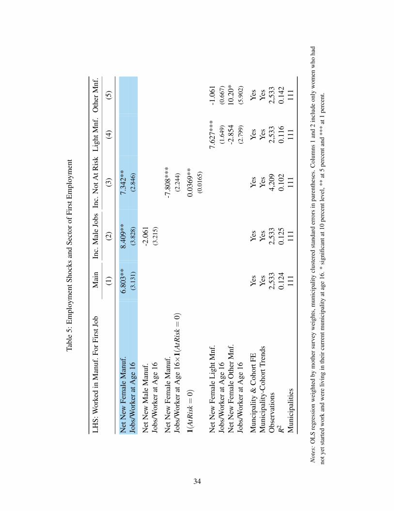
Tabl

e5:

Em

ploy

men

tSho

cks

and

Sect

orof

Firs

tEm

ploy

men

t

LH

S:W

orke

din

Man

uf.F

orFi

rstJ

obM

ain

Inc.

Mal

eJo

bsIn

c.N

otA

tRis

kL

ight

Mnf

.O

ther

Mnf

.

(1)

(2)

(3)

(4)

(5)

Net

New

Fem

ale

Man

uf.

6.80

3**

8.40

9**

7.34

2**

Jobs

/Wor

kera

tAge

16(3

.131

)(3

.828

)(2

.846

)

Net

New

Mal

eM

anuf

.-2

.061

Jobs

/Wor

kera

tAge

16(3

.215

)

Net

New

Fem

ale

Man

uf.

-7.8

08**

*Jo

bs/W

orke

ratA

ge16×

1(At

Ris

k=

0)(2

.244

)

1(At

Ris

k=

0)0.

0369

**(0

.016

5)

Net

New

Fem

ale

Lig

htM

nf.

7.62

7***

-1.0

61Jo

bs/W

orke

ratA

ge16

(1.6

49)

(0.6

67)

Net

New

Fem

ale

Oth

erM

nf.

-2.8

5410

.20*

Jobs

/Wor

kera

tAge

16(2

.799

)(5

.902

)

Mun

cipa

lity

&C

ohor

tFE

Yes

Yes

Yes

Yes

Yes

Mun

icip

ality

-Coh

ortT

rend

sY

esY

esY

esY

esY

esO

bser

vatio

ns2,

533

2,53

34,

209

2,53

32,

533

R2

0.12

40.

125

0.10

20.

116

0.14

2M

unic

ipal

ities

111

111

111

111

111

Not

es:

OL

Sre

gres

sion

wei

ghte

dby

mot

hers

urve

yw

eigh

ts,m

unic

ipal

itycl

uste

red

stan

dard

erro

rsin

pare

nthe

ses.

Col

umns

1an

d2

incl

ude

only

wom

enw

hoha

dno

tyet

star

ted

wor

kan

dw

ere

livin

gin

thei

rcur

rent

mun

icip

ality

atag

e16

.*si

gnifi

cant

at10

perc

entl

evel

,**

at5

perc

enta

nd**

*at

1pe

rcen

t.

34

Tabl

e7:

Red

uced

Form

Res

ults

LH

S:C

hild

Hei

ghtf

orA

geZ

scor

esM

ain

Con

trol

sM

ale

Man

uf.

Fem

ale

Man

uf.

Form

alJo

bsFe

mal

eSe

rvic

eSp

ecifi

catio

nJo

bsN

otA

tRis

kIn

tera

ctJo

bsJo

bs(1

)(2

)(3

)(4

)(5

)(6

)

Net

New

Fem

ale

Man

uf.

29.2

7**

25.4

6*51

.56*

**23

.18*

51.9

6***

30.0

5**

Jobs

/Wor

kera

tAge

16(1

4.29

)(1

3.38

)(1

4.03

)(1

2.52

)(1

6.23

)(1

3.86

)

Net

New

Fem

ale

Man

uf.

-27.

67**

-25.

53*

-40.

55**

-27.

13**

-45.

96**

*-2

8.59

**Jo

bs/W

orke

r×M

ale

Chi

ld(1

2.54

)(1

3.45

)(1

6.81

)(1

1.54

)(1

5.82

)(1

2.09

)

Net

New

xxxx

xxxx

x-2

8.97

**-3

2.95

**-1

0.90

**-1

7.68

Jobs

/Wor

kera

tAge

16(1

1.81

)(1

4.54

)(4

.339

)(1

4.50

)

Net

New

xxxx

xxxx

x15

.34

8.64

97.

935

9.02

9Jo

bs/W

orke

ratA

ge16×

Mal

eC

hild

(15.

88)

(41.

69)

(5.6

64)

(12.

38)

Mot

her’

sSc

hool

ing

atag

e16

0.01

50(0

.015

5)

Mot

her’

sH

eigh

t0.

0566

***

(0.0

0535

)

γm,s

ex,δ

c,δ

a,se

xFi

xed

Eff

ects

Yes

Yes

Yes

Yes

Yes

Yes

Mun

icip

ality

-Sex

-Chi

ldA

geTr

ends

Yes

Yes

Yes

Yes

Yes

Yes

Obs

erva

tions

3,01

82,

948

3,01

84,

292

3,01

83,

018

R2

0.31

70.

365

0.32

00.

266

0.31

90.

318

Mun

icip

aliti

es10

810

810

810

810

810

8

Not

es:

Reg

ress

ion

wei

ghte

dby

child

surv

eyw

eigh

ts,m

unic

ipal

itycl

uste

red

stan

dard

erro

rsin

pare

nthe

ses.

All

regr

essi

ons

incl

ude

only

wom

enw

how

ere

livin

gin

thei

rcur

rent

mun

icip

ality

atag

e15

exce

ptco

lum

n4

whi

chin

clud

esal

lwom

en.*

sign

ifica

ntat

10pe

rcen

tlev

el,*

*at

5pe

rcen

tand

***

at1

perc

ent.

35

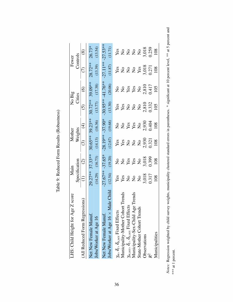
Tabl

e9:

Red

uced

Form

Res

ults

(Rob

ustn

ess)

LH

S:C

hild

Hei

ghtf

orA

geZ

scor

eM

ain

Mot

her

No

Big

Few

erSp

ecifi

catio

nW

eigh

tsC

ities

Con

trol

s(A

llR

educ

edFo

rmR

egre

ssio

ns)

(1)

(2)

(3)

(4)

(5)

(6)

(7)

(8)

Net

New

Fem

ale

Man

uf.

29.2

7**

37.3

3**

30.6

5**

39.2

3**

30.7

2**

39.0

9**

28.7

2**

26.7

3*Jo

bs/W

orke

ratA

ge16

(14.

29)

(16.

73)

(14.

13)

(16.

36)

(13.

77)

(17.

38)

(13.

39)

(13.

54)

Net

New

Fem

ale

Man

uf.

-27.

67**

-37.

65*

-28.

19**

-37.

90*

-30.

95**

-41.

76**

-27.

11**

-27.

53**

Jobs

/Wor

kera

tAge

16×

Mal

eC

hild

(12.

54)

(19.

20)

(12.

67)

(19.

68)

(13.

30)

(20.

06)

(11.

87)

(11.

71)

γm,δ

c,δ

a,se

xFi

xed

Eff

ects

Yes

No

Yes

No

Yes

No

Yes

Yes

Mun

icip

ality

-Mot

herC

ohor

tTre

nds

Yes

No

Yes

No

Yes

No

No

No

γm,s

ex,δ

c,δ

a,se

xFi

xed

Eff

ects

No

Yes

No

Yes

No

Yes

No

No

Mun

icip

ality

-Sex

-Chi

ldA

geTr

ends

No

Yes

No

Yes

No

Yes

No

No

Stat

e-M

othe

rCoh

ortT

rend

sN

oN

oN

oN

oN

oN

oY

esN

oO

bser

vatio

ns3,

018

3,01

82,

930

2,93

02,

810

2,81

03,

018

3,01

8R

20.

317

0.39

90.

321

0.40

40.

332

0.41

70.

271

0.25

9M

unic

ipal

ities

108

108

108

108

105

105

108

108

Not

es:

Reg

ress

ion

wei

ghte

dby

child

surv

eyw

eigh

ts,m

unic

ipal

itycl

uste

red

stan

dard

erro

rsin

pare

nthe

ses.

*si

gnifi

cant

at10

perc

entl

evel

,**

at5

perc

enta

nd**

*at

1pe

rcen

t.

36

Tabl

e11

:Hou

seho

ldB

arga

inin

gC

hann

els

LH

S:W

hoM

akes

Spen

ding

Dec

isio

ns?

Chi

ldE

duca

tion

Chi

ldH

ealth

Lar

geE

xpen

ditu

res

1=H

usba

nd,2

=Joi

nt,3

=Wif

e(1

)(2

)(3

)(4

)(5

)(6

)(7

)(8

)(9

)

Net

New

Fem

ale

Man

uf.

13.5

9**

13.0

1*14

.24*

11.7

4**

12.0

4**

14.2

2***

19.4

1**

19.1

5**

18.7

6*Jo

bs/W

orke

ratA

ge16

(6.7

88)

(7.0

26)

(8.1

94)

(5.0

31)

(5.0

74)

(4.8

90)

(9.5

65)

(9.6

14)

(10.

04)

Mot

herC

urre

ntly

Wor

ks0.

0776

**0.

0918

*-0

.040

9-0

.076

70.

0372

-0.0

349

(0.0

324)

(0.0

469)

(0.0

641)

(0.0

880)

(0.0

844)

(0.1

15)

Mot

hers

Cur

rent

Inco

me

-1.2

8e-0

62.

22e-

064.

32e-

06(P

esos

)(2

.11e

-06)

(1.7

8e-0

6)(3

.02e

-06)

Log

Hou

seho

ldC

onsu

mpt

ion

-0.0

148

-0.0

161

-0.0

143

PerC

apita

(Pes

os)

(0.0

473)

(0.0

375)

(0.0

509)

Hou

seho

ldSi

ze0.

0244

**0.

0205

-0.0

189

(0.0

113)

(0.0

135)

(0.0

164)

Obs

erva

tions

1,07

11,

071

1,02

51,

083

1,08

31,

037

1,07

81,

078

1,03

2R

20.

270

0.27

40.

280

0.22

50.

226

0.23

50.

237

0.23

80.

257

Mun

icip

aliti

es10

810

810

810

810

810

810

810

810

8

Not

es:

Reg

ress

ion

wei

ghte

dby

child

surv

eyw

eigh

ts,m

unic

ipal

itycl

uste

red

stan

dard

erro

rsin

pare

nthe

ses.

All

regr

essi

ons

incl

ude

only

wom

enw

hoha

dno

tyet

star

ted

wor

kan

dw

ere

livin

gin

thei

rcur

rent

mun

icip

ality

atag

e15

,hav

ehu

sban

dsat

hom

e,an

dha

vech

ildre

nin

the

mai

nhe

ight

fora

gesa

mpl

e.*

sign

ifica

ntat

10pe

rcen

tlev

el,*

*at

5pe

rcen

tand

***

at1

perc

ent.

37

Tabl

e13

:Ins

trum

ente

dR

egre

ssio

ns(T

wo

Stag

eL

east

Squa

res)

LH

S:C

hild

Hei

ghtf

orA

geZ

scor

esIV

OL

SR

FIV

OL

SR

F(1

)(2

)(3

)(4

)(5

)(6

)

Wor

ked

inM

anuf

.2.

327*

**0.

417*

1.81

0***

0.28

1Fi

rstJ

ob(0

.463

)(0

.240

)(0

.457

)(0

.189

)

Wor

ked

inM

anuf

.-1

.281

-0.3

49-1

.952

**-0

.289

Firs

tJob×

Mal

e(0

.822

)(0

.269

)(0

.781

)(0

.228

)

Net

New

Fem

ale

Man

uf.

38.4

2***

30.4

4**

Jobs

/Wor

kera

tAge

16(1

1.34

)(1

3.03

)

Net

New

Fem

ale

Man

uf.

-22.

39*

-26.

69**

Jobs

/Wor

kera

tAge

16×

Mal

e(1

1.70

)(1

1.99

)

γm,δ

c,δ

a,se

xFi

xed

Eff

ects

Yes

Yes

Yes

Yes

Yes

Yes

Mun

icip

ality

-Mot

herC

ohor

tTre

nds

Yes

Yes

Yes

Yes

Yes

Yes

Obs

erva

tions

2,41

22,

412

2,41

23,

014

3,01

43,

014

R2

0.27

60.

329

0.33

20.

275

0.31

40.

315

Mun

icip

aliti

es10

810

810

810

810

810

8C

ragg

-Don

ald

FSt

atis

tic29

.86

28.3

7

Not

es:

Reg

ress

ion

wei

ghte

dby

child

surv

eyw

eigh

ts,m

unic

ipal

itycl

uste

red

stan

dard

erro

rsin

pare

nthe

ses.

Col

umns

1to

3in

clud

eon

lyw

omen

who

had

noty

etst

arte

dw

ork

and

wer

eliv

ing

inth

eir

curr

entm

unic

ipal

ityat

age

15.

Col

umns

4to

6in

clud

eal

lwom

enw

how

ere

livin

gin

thei

rcu

rren

tmun

icip

ality

atag

e15

.*

sign

ifica

ntat

10pe

rcen

tlev

el,*

*at

5pe

rcen

tand

***

at1

perc

ent.

38

Tabl

e15

:Int

erac

tions

ofR

educ

edFo

rmw

ithSu

bsam

ples

LH

S:C

hild

Hei

ghtf

orA

geZ

scor

esM

anuf

.1st

Job

Not

AtR

isk

Infr

amar

gina

lIn

tera

ctio

nIn

tera

ctio

nW

orke

rsIn

tera

ctio

n(1

)(2

)(3

)(4

)(5

)(6

)

Net

New

Fem

ale

Man

uf.

0.20

89.

761

23.1

8*30

.85*

*35

.71*

*46

.61*

**Jo

bs/W

orke

ratA

ge16

(10.

85)

(11.

81)

(12.

52)

(15.

11)

(14.

06)

(15.

69)

Net

New

Fem

ale

Man

uf.

1.69

8-7

.344

-27.

13**

-31.

64*

-25.

93-4

0.98

*Jo

bs/W

orke

r×M

ale

Chi

ld(1

3.52

)(2

0.00

)(1

1.54

)(1

6.00

)(1

6.29

)(2

1.34

)

Net

New

Fem

ale

Man

uf.

55.3

3***

54.9

4***

-32.

95**

-35.

19**

-20.

50-2

9.18

Jobs

/Wor

kera

tAge

16r×

Inte

ract

ion

(10.

79)

(10.

92)

(14.

54)

(14.

13)

(18.

06)

(21.

48)

Net

New

Fem

ale

Man

uf.

-69.

95**

*-7

0.39

***

8.64

98.

762

-2.9

0013

.54

Jobs

/Wor

ker×

Mal

eC

hild×

Inte

ract

ion

(18.

76)

(17.

24)

(41.

69)

(44.

48)

(24.

04)

(30.

42)

γm,δ

c,δ

a,se

xFi

xed

Eff

ects

Yes

No

Yes

No

Yes

No

Mun

icip

ality

-Mot

herC

ohor

tTre

nds

Yes

No

Yes

No

Yes

No

γm,s

ex,δ

c,δ

a,se

xFi

xed

Eff

ects

No

Yes

No

Yes

No

Yes

Mun

icip

ality

-Sex

-Chi

ldA

geTr

ends

No

Yes

No

Yes

No

Yes

Obs

erva

tions

3,01

43,

014

4,29

24,

292

3,01

83,

018

R2

0.32

00.

404

0.26

60.

338

0.31

70.

400

Mun

icip

aliti

es10

810

810

810

810

810

8

Not

es:

Reg

ress

ion

wei

ghte

dby

child

surv

eyw

eigh

ts,m

unic

ipal

itycl

uste

red

stan

dard

erro

rsin

pare

nthe

ses.

All

regr

essi

ons

incl

ude

only

wom

enw

how

ere

livin

gin

thei

rcur

rent

mun

icip

ality

atag

e15

exce

ptco

lum

ns3

and

4.*

sign

ifica

ntat

10pe

rcen

tlev

el,*

*at

5pe

rcen

tand

***

at1

perc

ent.

39

Endogenous Skill Acquisition and Export Manufacturing in Mexico∗

David Atkin†

April 2011

Abstract

Studies based on firm-level data find that both exporting firms and multinational corporations

pay higher wages for a given skill level. However, the literature overlooks the fact that export

manufacturing firms may also change the educational choices of the workforce. In this paper, I

confirm that for Mexico during the period 1986-2000, the export sector pays higher wages than

other sectors, but school drop out increases with the arrival of new export jobs. By the year 2000,

the workers induced to enter export manufacturing are earning less than they would have earned

had the jobs never appeared and they stayed in school longer. I identify the causal effects by

looking within municipalities and examining how the education of different cohorts varies with

new factory openings in the municipality at key school-leaving ages. Export manufacturing attracts

students by paying high relative wages for unskilled workers, and offering many jobs to low-skill

workers straight out of school. The magnitudes I find suggest that for every ten new jobs created,

one student drops out of school at grade 9 rather than continuing on through grade 12.

JEL Codes: F16, J24, O12, O14, O19

∗Special thanks to David Kaplan at ITAM for computing and making available the IMSS Municipality level employmentdata. Thanks to Angus Deaton, Penny Goldberg and Gene Grossman for guidance and encouragement throughout.Further thanks to Joe Altonji, Treb Allen, Chris Blattman, Richard Chiburis, Dave Donaldson, Marco Gonzalez-Navarro,Leonardo Iacovone, Amit Khandelwal, Fabian Lange, Adriana Lleras-Muney, Marc Melitz, Mushfiq Mobarak, Marc-Andreas Muendler, Hannah Pitt, Guido Porto, Nancy Qian, Jesse Rothstein, Sam Schulhofer-Wohl, Eric Verhoogen, threeanonyomous referees and seminar participants at Princeton, the 15th BREAD conference, the 1st LACEA TIGN conference,the 2010 NBER summer institute and Yale for their useful comments. Financial aid from the Fellowship of WoodrowWilson Scholars at Princeton University is gratefully acknowledged. Any errors contained in the paper are my own.†Yale University Department of Economics, BREAD, CEPR and NBER. E-mail: david.atkin@yale.edu

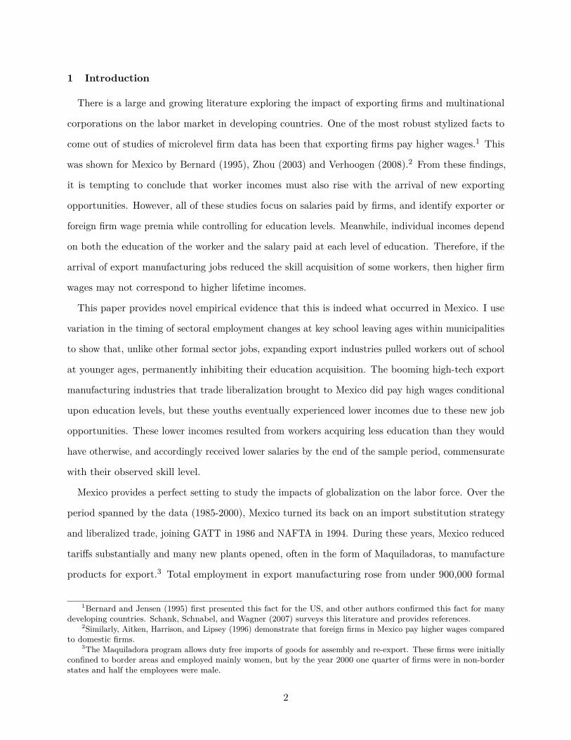
1 Introduction

There is a large and growing literature exploring the impact of exporting firms and multinational

corporations on the labor market in developing countries. One of the most robust stylized facts to

come out of studies of microlevel firm data has been that exporting firms pay higher wages.1 This

was shown for Mexico by Bernard (1995), Zhou (2003) and Verhoogen (2008).2 From these findings,

it is tempting to conclude that worker incomes must also rise with the arrival of new exporting

opportunities. However, all of these studies focus on salaries paid by firms, and identify exporter or

foreign firm wage premia while controlling for education levels. Meanwhile, individual incomes depend

on both the education of the worker and the salary paid at each level of education. Therefore, if the

arrival of export manufacturing jobs reduced the skill acquisition of some workers, then higher firm

wages may not correspond to higher lifetime incomes.

This paper provides novel empirical evidence that this is indeed what occurred in Mexico. I use

variation in the timing of sectoral employment changes at key school leaving ages within municipalities

to show that, unlike other formal sector jobs, expanding export industries pulled workers out of school

at younger ages, permanently inhibiting their education acquisition. The booming high-tech export

manufacturing industries that trade liberalization brought to Mexico did pay high wages conditional

upon education levels, but these youths eventually experienced lower incomes due to these new job

opportunities. These lower incomes resulted from workers acquiring less education than they would

have otherwise, and accordingly received lower salaries by the end of the sample period, commensurate

with their observed skill level.

Mexico provides a perfect setting to study the impacts of globalization on the labor force. Over the

period spanned by the data (1985-2000), Mexico turned its back on an import substitution strategy

and liberalized trade, joining GATT in 1986 and NAFTA in 1994. During these years, Mexico reduced

tariffs substantially and many new plants opened, often in the form of Maquiladoras, to manufacture

products for export.3 Total employment in export manufacturing rose from under 900,000 formal

1Bernard and Jensen (1995) first presented this fact for the US, and other authors confirmed this fact for manydeveloping countries. Schank, Schnabel, and Wagner (2007) surveys this literature and provides references.

2Similarly, Aitken, Harrison, and Lipsey (1996) demonstrate that foreign firms in Mexico pay higher wages comparedto domestic firms.

3The Maquiladora program allows duty free imports of goods for assembly and re-export. These firms were initiallyconfined to border areas and employed mainly women, but by the year 2000 one quarter of firms were in non-borderstates and half the employees were male.

2

sector jobs at the beginning of 1986 to over 2.7 million jobs in 2000. Much of this growth was driven

by multinational corporations, with nearly two thirds of manufacturing exports in 2000 originating

from foreign affiliates (UNCTAD 2002). In this paper, I demonstrate that this massive expansion

in export manufacturing altered the education decisions of Mexico’s youth.4

A simple conceptual framework guides the empirical work. I modify a Becker (1962) human capital

model to include stochastic job opportunities that offer persistent wage premia.5 I find that my

results are consistent with such a modification.6 This framework illustrates that new employment

opportunities have two offsetting effects. On the one hand, when a new firm opens, a student may

drop out of school, expecting to be better off by taking the new job rather than by chancing the job

market with more education in the future—the opportunity cost of schooling channel.7 On the other

hand, if the student expects that vacancies will continue to be available and these jobs will sufficiently

reward skill acquisition, she may choose to stay in school longer—the returns to schooling channel.

The net effect of these two channels depends on the wage and availability of jobs at different skill

levels in that firm and the likelihood that there will also be vacancies in the future. For example,

the student is more likely to drop out of school if the firm is predominantly hiring unskilled workers at

attractive wages and does not anticipate hiring a substantial number of additional workers in future.

In this paper, I find that the characteristics of export manufacturing firms place them in the former

category, in which new job arrivals induce school dropout. The magnitudes I find suggest that for every

ten high-tech export jobs that arrived, one student dropped out at grade 9 rather than continuing

on through grade 12. In contrast, the arrival of new non export manufacturing and service jobs induce

greater skill acquisition. The most likely explanation is that, compared to the other industries, export

manufacturing offers an abundance of low-skill jobs that pay relatively high wages to workers with low

levels of schooling. Additionally, job vacancies in the export manufacturing industry are the least likely

to persist into the future. Therefore, an influx of such jobs raises the opportunity cost of schooling

4Most of my analysis relates to youths deciding how much secondary school to obtain, the relevant margin forexport manufacturing jobs in Mexico where 80 percent of employees had less than 12 years of schooling in the year 2000.

5These wage premia originate from well-documented firm and cohort-specific non-compensating wage differentials.6In a neoclassical labor market setting, job flows only affect education decisions by changing the relative demand

for skill. However, I find several result that are inconsistent with the neoclassical labor market model. In this sense,the paper relates to recent work that explores the impacts of trade in non-neoclassical labor market settings. See forexample, Davis and Harrigan (2007) and Helpman, Itskhoki, and Redding (2008). Frias, Kaplan, and Verhoogen (2009)provides empirical evidence on the importance of these non-neoclassical features.

7In this paper, I use the term drop out to refer to leaving school at any point when additional educational attainmentis possible.

3

for youths to a larger degree than the returns to schooling. Consistent with this interpretation, I find

that once these industry characteristics are controlled for, new jobs in export-intensive sectors actually

encourage students to stay in school relative to similar industries.8

A unique data set makes this analysis possible. I merge firm-level employment data for the universe

of formal sector firms with 10 million schooling records from the 2000 Mexican census. These data only

allow me to focus on one component of human capital, schooling.9 Accordingly, I match each cohort’s

average education to the job growth in their municipality at ages 15 and 16, the age at which compulsory

education concludes and formal employment is first possible. Having cohort-specific schooling and

local employment measures at a very disaggregated level allows me to look within 1,808 municipalities

and plausibly identify the causal impacts of job availability on education decisions in Mexico.

I compare cohorts within a municipality who reached their key school leaving age at the time of sub-

stantial factory openings to slightly younger or older cohorts who did not. The main empirical difficulty

is reverse causation; that local skill levels may determine formal firm employment decisions. To address

this issue, I instrument for job growth with large factory openings/expansions or closings/contractions.

My strategy assumes that the decision for a firm to open/expand or close/contract a factory in a

region is not an outcome of cohort-specific changes in the local labor supply. This assumption seems

reasonable as such sizable expansions or contractions are associated with large fixed costs and are

not plausibly driven by changes in the labor supply of a single cohort of youths. This is especially true

in Mexico, where a large quantity of migrant and informal labor ensures that changes in the dropout

decisions of a single cohort comprise a very small part of the potential labor that a firm can hire.10

In this paper, I focus on educational acquisition. Clearly there are other dimensions of skill. For

example, export firms may offer on-the-job training which is more valuable to workers than additional

years of schooling. Accordingly, I also investigate the impact of these educationl decision on earned

income in the final year of my sample period. It is a well-known stylized fact that exporting firms pay

higher wages, conditional on education levels.11 However, I find that despite the high wages on offer

8However, the fact that export manufacturing firms use low-skill labor intensively is not a coincidence. TheHeckscher-Ohlin theorem predicts that Mexico will export products intensive in this relatively abundant factor.

9New firm arrivals may induce skill acquisition through other means, e.g. on the job training (Acemoglu andPischke 1998) or knowledge spillovers (Keller 2004).

10The informal sector comprises between one third and two thirds of Mexican employment. Around 20 percentof my sample are migrants. In this paper, I focus only on non-migrants, and results pertain only to that group.

11Schank, Schnabel, and Wagner (2007) surveys this literature and provides references. This fact was shown forMexico by Bernard (1995), Zhou (2003) and Verhoogen (2008). All of these studies focus on salaries paid by firms,and identify exporter or foreign firm wage premia while controlling for education levels.

4

in this sector, earned incomes in the year 2000 are still lower for the youths induced to forgo education

by new export opportunities, commensurate with their lower schooling levels. Any additional skills

that these cohorts acquired out of the schooling system were insufficient to monetarily compensate

for the lower schooling levels, at least by the year 2000.

This paper provides evidence that lends support to models of trade with endogenous skill acquisition.

For example, Findlay and Kierzkowski (1983) incorporates human capital decisions into a Heckscher-

Ohlin model and shows that trade exacerbates initial skill differences across countries by raising the

return to the abundant skill—the Stolper–Samuelson effect—exactly as I find.12 Trade can induce diver-

gent growth paths if positive externalities to education are incorporated into such a model (Stokey 1991).

My findings are consistent with the literature on trade and wages in Mexico. The various stages

of trade liberalization in Mexico have been associated with an initial rise in the skill premium until

the mid 1990’s, followed by a skill premium decline.13 My schooling results follow a similar inverse-U

pattern with time. The reduction in schooling from new export manufacturing jobs primarily occurred

with job arrivals in the latter period of my sample, a time when returns to high school were falling.

It should be noted that new export manufacturing jobs can increase school dropout even if they raise

the high-skill to low-skill wage ratio. Risk averse or impatient youths may rationally choose a newly

available low-skill export job today over more schooling and the (uncertain) possibility of a high-paying

high-skill export job in future.14

The results are also consistent with the findings of studies in labor economics. Several studies use

panels of region or state-level unemployment rates to show that students stay in school longer during

a recession.15 In the development context, Goldin and Katz (1997) show that industrialization slowed

educational growth in the early 20th century United States, while Federman and Levine (2005) and

Le Brun, Helper, and Levine (2009) find industrialization increased enrollments in Indonesia and had

mixed effects in Mexico.16

12Ambiguous results obtain when credit constraints are introduced to such a model (Chesnokova and Krishna 2009).13This is a large literature including Cragg and Epelbaum (1996), Hanson and Harrison (1999), Feenstra and Hanson

(1997), Robertson (2004), Airola and Juhn (2005) and Lopez-Acevedo (2006). Verhoogen (2008) finds skill upgradingwithin non-Maquiladora exporters in the mid 1990’s.

14The probability of obtaining a high-skill export job may be quite small as 85 percent of formal sector employeesin my two export industries (defined in section 3.1) have less than a high school education. In reality, youths are likelyto be trading off a job in manufacturing if they dropout of school for a job in services if they acquire more education.

15See Card and Lemieux (2000) and Kahn (2007) for the US and Clark (2009) for the UK.16Le Brun, Helper, and Levine (2009) compare municipality education changes between the 1990 and 2000 with

total manufacturing growth over that period. Manufacturing growth is associated with increased education for youngerchildren but reduced education for girls aged 16 to 18.

5

Finally, a complementary recent literature looks at the educational impacts of the arrival of IT

service jobs in India. Munshi and Rosenzweig (2006), Shastry (2008), ? and Oster (2010) all find

positive enrollment impacts from the arrival of relatively high-skilled service job opportunities in India.

Such opportunities raised the returns to education, and similarly, I observe that new formal-sector

service jobs increase education acquisition in Mexico. However, India’s experience may be regarded as

the exception rather than the rule, as it is far more common for a developing country to have a revealed

comparative advantage in low-skill manufacturing rather than comparatively high-skill services.

This paper improves on the existing studies in several ways. First, by drawing on a richer data set to

assemble a very large panel (1,808 municipalities) and by using an instrumentation strategy, I am able to

control for potential reverse causality that comes from endogenous firm location choices. Second, these

rich data allow me to separately identify the educational impacts of local job availability across all formal

sector industries. Third, guided by my conceptual framework, I am able to separate the educational

impact of periods of job declines from periods of job growth and to identify the industry characteristics

that determine whether new job arrivals either encourage or discourage additional schooling.17

My findings have important, albeit nuanced, policy implications for Mexico and many other countries.

From an individual perspective, my results are entirely consistent with rational and perfectly informed

youths choosing to take a good job opportunity when it arrives. However, from a macro perspective,

many countries pursuing export-led growth strategies also want to upgrade the skill level of their work-

force, believing that the positive externalities from education drive long-run growth rates (Lucas 1988). I

show that there is a tradeoff between these two goals, at least in the Mexican context, as the export man-

ufacturing firms attracted by such strategies possessed characteristics that discouraged skill acquisition.

The next section lays out the conceptual framework. Section 3 introduces the rich data set and

discuss the methodology. Section 4 presents the basic regression results, and robustness checks are

shown in section 5. Section 6 uses the conceptual framework to explain why I find that only export

manufacturing jobs induce school dropout. Section 7 looks at income effects. Finally, section 8

discusses policy implications and concludes. Appendix A explores potential biases due to migration.

17My conceptual framework suggests that such an asymmetry may be present during this time period if studentscorrectly predicted that periods of job declines were likely to reverse, yet periods of growth were likely to continue.

6

2 A Conceptual Framework for Understanding Educational Choices

I briefly discuss a conceptual framework that clarifies the channels through which new employment

opportunities in different industries affect a student’s education choice. In a standard education

decision model, a student trades off the higher future wage profile available to more educated workers

for the immediate income that employment today brings. If the student has a sufficiently high discount

rate, she will rationally decide to drop out of school and start earning despite knowing that her wage

will be lower in future. In a neoclassical labor market setting, new job arrivals will increase the demand

for the types of labor that those particular jobs require and alter the relative attractiveness of the

skilled and unskilled wage profiles. Thus, new job arrivals in two industries that demand a similar

distribution of skills should have identical effects on the student’s schooling decision. My empirical

findings are inconsistent with this prediction. I find that new export manufacturing job opportunities

encourage students to drop out of school, while new opportunities in other similarly skilled sectors

encourage additional schooling. Therefore, in order to highlight the industry characteristics that can

induce such heterogeneity in the response of education to new job opportunities, I outline a decision

making-process in the context of stochastic job vacancies.

First, I describe a stylized decision making process. A forward-looking student must make two

sequential decisions: whether to drop out of school; and if he or she drops out of school, which industry

i to enter. For clarity in this simplified exposition, I will assume both decisions are irreversible, although

I can easily relax this assumption without altering the main implications.18 If a student drops out

of school at t, with s years of schooling and enters industry i, she receives income εistyis,τ−t for each

year τ thereafter. A stochastic year-of-entry wage premium εist is multiplied by an historic industry

wage profile, yis,τ−t, that does not depend on the year of entry.19 The year-of-entry wage premium

summarizes the job vacancies in the industry available to a particular student in a given year. These

year-of-entry wage premia exist as only certain firms will offer a particular worker a job in any given

year. If the student receives no job offers in that industry that year, then εist = 0. The formal sector

of employment in Mexico is characterized by firm-specific non-compensating wage differentials and job

18Relaxing the assumption of irreversible school dropout reduces the option value of staying in school and so increasesdropout when new jobs arrive. Incorporating job separations into the model reduces dropout with new jobs arrive sincea student can change job and industry in future if better opportunities arise. In this case, equation 1 should be expressedwith value functions that include the possibility of returning to school or changing industry in future, both at some cost.

19The historic industry wage profile depends only on education, s, and experience, τ − t.

7

rationing.20 Therefore, the wage a worker receives will depend on which firm hires her.21 In a year when

more firms are hiring and more vacancies are posted, a student is more likely to be able to obtain a job at

a firm that pays persistently higher wages.22,23 Accordingly, the year-of-entry wage premium is a weakly

increasing function of the net new jobs, lit, created in industry i that year; εist = εis(lit), ε′is(lit) ≥ 0.

The education decision corresponds to an optimal stopping model. The student decides whether

to take the best job available or to wait one more period and choose again. If she waits, she consumes

the at-school income equivalent, yt, and retains the option to choose again next period with one more

year of schooling, when there may also be more firms hiring.24 The student cannot borrow or save,

discounts at the rate ρ and has constant relative risk aversion utility with risk aversion parameter

σ. For simplicity, I assume that the student makes a binary schooling choice of either dropping out

of school at time t (s = 0) or completing high school at time t+ 1 (s = 1):

s = I[maxi∈I

(εi0(lit)1−σ∞∑τ=t

y1−σi0,τ−t

(1 + ρ)τ−t ) < y1−σt + Et[max

i∈I(εi1(lit+1)1−σ

∞∑τ=t+1

y1−σi1,τ−t−1

(1 + ρ)τ−t )]]. (1)

The student stays in school if the net present value of the best job available today across industries

(the “opportunity cost of schooling”) is inferior to the expected net present value of the best future job

plus the utility during the year of school attendance (the “returns to schooling”).25 The opportunity

cost of schooling is not only the foregone earnings if the student stays at school, but also includes

the potential loss from turning down a job at a firm that pays high wage premia and may not be

hiring the following year.

20Frias, Kaplan, and Verhoogen (2009) document firm-specific wage differentials in Mexico, presumably only possibleif firms ration the number of jobs they offer. Duval Hernandez (2006) presents evidence of more general formal sectorjob rationing in Mexico. However, Maloney (2004) suggests that the least skilled may prefer self-employment to the worstformal sector jobs, although this does not seem to be the case higher up the skill distribution (Gong and van Soest 2002).

21These firm-specific premia may derive from efficiency wage models (Shapiro and Stiglitz 1984), fair wageconsiderations (Akerlof and Yellen 1990), search models where high productivity firms find vacancies more costly (Burdettand Mortensen 1998), insider bargaining (Abowd and Lemieux 1993) or external pressures from foreign consumers(Harrison and Scorse forthcoming).

22Oreopoulos, Von Wachter, and Heisz (2006) present evidence for year-of-entry wage premia in Canada.23Even for a given firm, there may be wage premia that depend on the labor demand conditions during the year

of entry into that firm. Beaudry and DiNardo (1991) show that, within firms, a persistant cohort-specific wage premiumemerges endogenously from optimal lifetime contracts for risk-averse credit-constrained workers.Baker, Gibbs, andHolmstrom (1994) provide evidence for such "handshake" models.

24The at-school income equivalent depends on family support, the disutility or cost of school attendance and part-timeemployment opportunities.

25A high discount rate or low at-school income will generally reduce the desire for additional schooling as the netbenefits of schooling are smaller and are discounted more heavily. Meanwhile, high risk aversion increases the probabilityof dropout in response to new job opportunities because the student values uncertain future vacancies relatively lessthan certain vacancies today.

8

I now explore how new job arrivals in industry i affect the schooling decision. In the simplest case, new

jobs arrivals, lit, weakly reduce schooling by weakly raising the best wage on offer if the student drops-out

today.26 However, the realization of net new jobs today may change the expected industry year-of-entry

wage premium in the future, Etεi1(li,t+1). For example, a new factory-opening brings many immediate

vacancies, but students may expect the factory to hire additional workers next year or more firms to ar-

rive in the future due to the forces of agglomeration or industry growth. If lit is positively correlated with

Etεi1(li,t+1), both the best job available today and the expected best future job may change and the net

impact on schooling will be ambiguous. The next two sections of the paper use a reduced form empirical

approach to determine the sign of the net effect of new job arrivals on schooling for each industry.

The perceived serial correlation of new jobs provides an additional empirical prediction that dif-

ferentiates an education decision framework in a neoclassical labor market setting from one in which

vacancies are stochastic. In neoclassical labor market settings, new job arrivals in a high skill industry

should raise the returns to schooling by increasing the demand for skill and making skill acquisition

more attractive. Correspondingly, job losses in this industry should reduce the demand for skill and

increase the incentive to dropout. However, in a framework with stochastic vacancies, the perceived

serial correlation may be a function of net new jobs. In Mexico, most years between 1986 and 2000

saw substantial formal sector employment growth. Consequently, lit and li,t+1 were uncorrelated if

lit < 0 but positively correlated if lit > 0. If students had expectations consistent with this pattern,

both job arrivals and job losses in a high skill industry will encourage students to stay in school. In

the latter case, jobs in the sector are unavailable today so the opportunity cost of schooling falls, but

students still expect them to be available in the future. I test this conjecture in section 4.1, and find

evidence in favor of an education decision framework that incorporates stochastic vacancies.

2.1 Industry Characteristics and School Dropout

There are three observable industry characteristics that determine whether new jobs at time t in

industry i encourage or discourage school dropout in a framework with stochastic vacancies.

First, the lower the perceived serial correlation between new jobs arriving today, lit, and new jobs ar-

riving in future, li,t+1, the more likely it is that new jobs in industry i will encourage school dropout. The

expected net present value of the best job in future in that industry will improve by only a small amount

26Adding a cost to job searching makes dropout more tempting when new jobs arrive since the search costs willbe lower that year.

9

if students perceive a low positive serial correlation and will deteriorate for a negative serial correlation.

For the next two industry characteristics that I will describe, I assume that students expect a

positive correlation between new jobs today and new jobs in future.

Second, the higher the wages for school dropouts in industry i compared to other industries, the

more likely it is that one of the new jobs in industry i is the best job available to the student today,

raising the opportunity cost of schooling. Conversely, the higher the wages for school graduates in

industry i compared to other industries, the larger the increase in the expected best future job and

the perceived returns to schooling. Therefore, the higher the ratio between these two relative wage

terms, the more likely it is that new jobs in industry i encourage school dropout.27

Third, the higher the proportion of employees that are school dropouts in industry i compared

to other industries, the more likely it is that the vacant positions do not require high school education.

Therefore, a job opening in industry i is more likely to be the best job available to the student today,

raise the opportunity cost of schooling and encourage school dropout. By a similar logic, the higher

the proportion of vacancies that are filled by young and inexperienced workers in industry i, the more

likely job openings in industry i are to encourage school dropout.

In summary, whether a new job arrival in a particular industry does discourage education acquisition

will depend in part on the three industry characteristics: the serial correlation of new job openings,

the relative wage premia paid to different skill levels and the availability of jobs at different skill

levels. Only the last of these characteristics matters in a standard neoclassical labor market setting.

In section 6, I evaluate the importance of these three characteristics in explaining the heterogenous

educational effect of new jobs that I find across industries.

3 Empirical Implementation

3.1 Data

I use two sources of data in this paper to examine how the education of different age cohorts in

a municipality varies with new job opportunities in different industries. The education data are from

a 10.6 percent subsample of the 2000 Mexican decennial census collected by the National Institute

of Statistics, Geography, and Informatics (INEGI).28 The 10.1 million person records cover all 2,44327E.g. New jobs in industry i are more likely to encourage dropout when the wage for school dropouts relative

to other industries divided by the wage for school graduates relative to other industries is large.28The census, XIII Censo General de Poblacion y Vivienda 2000, is publicly available from IPUMSI Minnesota

Population Center (2007). I obtain the annual working-age municipality population by linearly interpolating INEGI

10

municipalities in Mexico. Data from the 1990 census are also used to investigate various industry

characteristics. I cannot, unfortunately, use family background data for the individuals, as many of

the older cohorts I study have left their parental homes by the time of the census.

The employment data originate from the Mexican Social Security Institute (IMSS), and cover the

complete universe of formal private-sector establishments, including Maquiladoras. IMSS provides

health insurance and pension coverage and all employees must enroll. I construct the main employment

variable, net new jobs, from annual changes in employment by industry within each municipality.29 The

data cover 2.2 million firms between 1985 and 2000, with annual employment recorded on December

31st of each year. Sample means for both data sources are shown in table 1.

As this paper focuses on the impact of export-oriented manufacturing, I break the manufacturing

sector into export and non export industries. The IMSS data assigns each firm to an industry category,

but does not indicate whether it exports or not. Therefore, I define a firm as an exporter if it belongs

to a 3-digit ISIC classification (Rev. 2) industry where more than 50 percent of output was exported

for at least half the years in the sample.30 The conceptual framework suggests that new jobs in

high-skill and low-skill industries may produce quite different educational outcomes. Therefore, I split

the very heterogenous export manufacturing and service sectors by the average education of the 3-digit

industry’s employees in the 2000 census.

The composition and sizes of the five industry groupings are as follows:31 Non Export Manufacturing

(1,087,457 jobs in Metals, Minerals, Glass, Plastics, Chemicals, Paper, Publishing, Food, Beverage and

Tobacco), Low-Tech Export Manufacturing (898,592 jobs in Textiles, Apparel, Shoes, Leather, Wood

and Furniture), High-Tech Export Manufacturing (1,396,645 jobs in Electrical, Electronic, Transport

and Scientific Equipment; Toys, Clocks and Ceramics), Commerce and Personal Services (3,066,358

jobs in Communications, Rental, Food, Lodging, Domestic, Recreational and Transport Services) and

Professional Services (1,733,037 jobs in Professional, Technical, Medical, Educational, Administrative

and Financial Services). The skill distribution of workers in these industries in 2000 is shown in

population data for ages 15-49 from 1990, 1995 and 2000.29The aggregations from the firm to municipality level were carried out at ITAM, where the data is held securely.

Kaplan, Gonzalez, and Robertson (2007) contains further details on the IMSS data.30The industry categories used by IMSS, the 2000 census and the 3-digit ISIC classification (Rev. 2) were matched

by hand. The export and output data come from the Trade, Production and Protection 1976-2004 database (Nicitaand Olarreaga 2007). Results are robust to using other export industry groupings.

31The size is the total employment in the year 2000 from the IMSS database, excluding the Mexico City metropolitanarea.

11

figure 3.32 The low-tech export manufacturing sector is substantially less skilled than the two other

manufacturing sectors, which in turn are less skilled than the service sectors.

While not all of the jobs in the industries that I classify as high and low-tech export manufacturing

are in firms that export, the overwhelming majority are. Of the approximately 2.3 million jobs in these

two industries in 2000, about 1.2 million are in Maquiladoras. Maquiladoras can import intermediates

duty free, and are required to export most of their production. This type of firm accounted for more

than half the employment growth over the period. A large number of the remaining 1.1 million jobs are

also in exporting firms. In the 1990 Encuesta Industrial Anual, which only covers large non-Maquiladora

firms, half of the 417,000 jobs in these two industries were in firms that exported. This proportion

is likely to have increased further as Mexican manufacturing became more export oriented over the

1990’s. Figure 1 and 2 provide more details about the manufacturing firm groupings. Firms in the two

export manufacturing sectors export a much larger fraction of their total output and are more likely to

be Maquiladoras or foreign owned.33 A substantial fraction of the year on year growth in employment

in the export industries is driven by Maquiladoras, particualrly in the middle of 1990’s. In section 6, I

explore whether new Maquiladora jobs affect education choices differently than other new jobs. To do

this, I approximately identify the Maquiladora firms in my sample by matching firm level employment

data to INEGI aggregate statistics on Maquiladoras by industry, state-industry and municipality.34

I combine the education and employment data using the 1985 municipal boundaries. In order for

each location to represent a single labor market, I merge any municipalities classified by INEGI as

metropolitan zones or where more than 10 percent of the working population commute to a nearby

municipality.35 These adjustments result in a panel of 13 cohorts across 1,809 municipalities.36

32The education distribution is calculated using IMSS insured workers in the year 2000 census.33These data cover the whole of Mexico and originate from Banco de Mexico, Nicita and Olarreaga (2007) and

Ibarraran (2004). The measure of output used by Nicita and Olarreaga (2007) does not properly account for allthe imported intermediate components that typify the Mexican export production, hence the major export assemblyindustries show export ratios of over 100 percent.

34These data come from http://dgcnesyp.inegi.gob.mx/cgi-win/bdieintsi.exe. I am able to roughly identifyMaquiladoras by classifying a firm as a Maquiladora when the number of firms or employees in a given aggregate cellis equal in the INEGI data to the number of firms or employees in the IMSS dataset. The fact that each of these firmsappear in several overlapping aggregates allows me to iterate this process until convergence. Due to the highly clusterednature of Maquiladora production in Mexico, I am able to classify all the potential Maquiladoras in 4 iterations.

35I make this correction as if workers commute to nearby municipalities, the error terms will be spatially correlated.When a municipality sends workers to two different municipalities that do not send workers to each other, two syntheticmunicipalities are created, with both containing the sending municipality (but with its relative weighting halved).

36To calculate changes in employment, I lose the first year of data, 1985. Since the census was collected in February2000, only firm data through 1999 is relevant. This leaves 14 years of data, but the two-year exposure window reducesthe length of the panel to 13 cohorts.

12

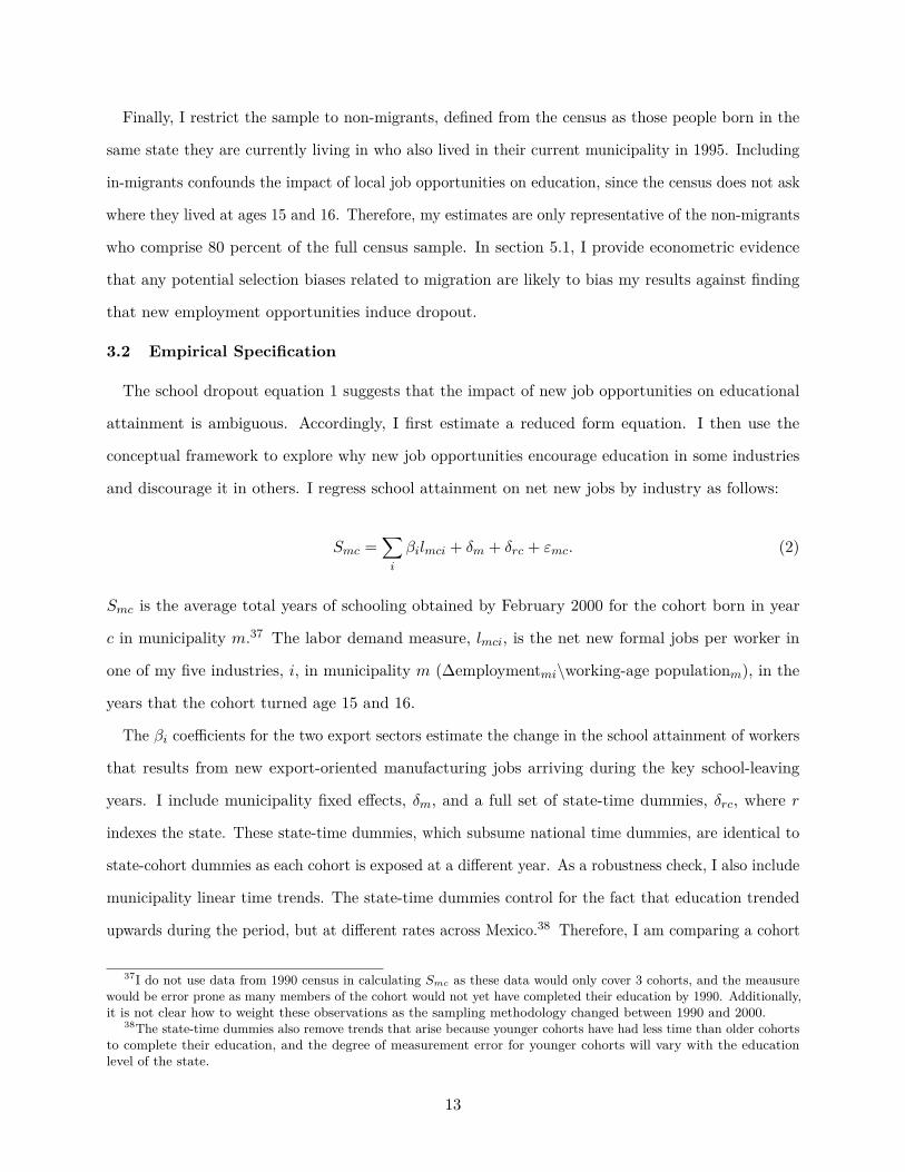
Finally, I restrict the sample to non-migrants, defined from the census as those people born in the

same state they are currently living in who also lived in their current municipality in 1995. Including

in-migrants confounds the impact of local job opportunities on education, since the census does not ask

where they lived at ages 15 and 16. Therefore, my estimates are only representative of the non-migrants

who comprise 80 percent of the full census sample. In section 5.1, I provide econometric evidence

that any potential selection biases related to migration are likely to bias my results against finding

that new employment opportunities induce dropout.

3.2 Empirical Specification

The school dropout equation 1 suggests that the impact of new job opportunities on educational

attainment is ambiguous. Accordingly, I first estimate a reduced form equation. I then use the

conceptual framework to explore why new job opportunities encourage education in some industries

and discourage it in others. I regress school attainment on net new jobs by industry as follows:

Smc =∑i

βilmci + δm + δrc + εmc. (2)

Smc is the average total years of schooling obtained by February 2000 for the cohort born in year

c in municipality m.37 The labor demand measure, lmci, is the net new formal jobs per worker in

one of my five industries, i, in municipality m (∆employmentmi\working-age populationm), in the

years that the cohort turned age 15 and 16.

The βi coefficients for the two export sectors estimate the change in the school attainment of workers

that results from new export-oriented manufacturing jobs arriving during the key school-leaving

years. I include municipality fixed effects, δm, and a full set of state-time dummies, δrc, where r

indexes the state. These state-time dummies, which subsume national time dummies, are identical to

state-cohort dummies as each cohort is exposed at a different year. As a robustness check, I also include

municipality linear time trends. The state-time dummies control for the fact that education trended

upwards during the period, but at different rates across Mexico.38 Therefore, I am comparing a cohort

37I do not use data from 1990 census in calculating Smc as these data would only cover 3 cohorts, and the meausurewould be error prone as many members of the cohort would not yet have completed their education by 1990. Additionally,it is not clear how to weight these observations as the sampling methodology changed between 1990 and 2000.

38The state-time dummies also remove trends that arise because younger cohorts have had less time than older cohortsto complete their education, and the degree of measurement error for younger cohorts will vary with the educationlevel of the state.

13

within a municipality who was heavily exposed to new factory openings at their key school leaving

age to other cohorts in the same municipality who did not have such a shock to their employment

opportunities at these ages, flexibly controlling for time effects using the cohorts of key school-leaving

age in nearby municipalities where factories did not open. In section 3.3, I discuss potential reverse

causation and omitted variable bias in detail, and present a novel instrumentation strategy.

The addition of state-time dummies means that the Valle de México metropolitan zone (that includes

Mexico City) is essentially omitted from my sample as it constitutes two states on its own. As a

robustness check, in section 5, I include region-time dummies for six regions of Mexico instead of

state-time dummies.

The main specification focuses on new jobs arriving at ages 15 and 16, although I will also examine

other exposure ages. Compulsory schooling in Mexico ends with Secundaria (grade 9), and most

children complete this grade at either 15 or 16 depending on their birth date. The compulsory schooling

law only dates from 1992 and enforcement is rare (Behrman, Sengupta, and Todd 2005). However,

ages 15 and 16 are still the two most common school leaving ages and the age at which the decision

to attend high school is made. Additionally, formal sector jobs first become a direct alternative to

school at this age, as the minimum formal sector working age is 16.3940

3.3 Empirical Methodology and Threats to Identification

With a conceptual framework in place and the basic specification introduced, I now address the

three main econometric concerns: omitted variables, measurement error and reverse causality. Omitted

variables will bias coefficients if a third factor affects both a municipality’s education level and its

attractiveness as a location for a firm.41 Using the panel dimension of my data, I am able to sweep

out time-invariant features of the municipality using municipality fixed effects. Similarly, the flexible

state-time dummies control for any omitted variable that changes over time within the 32 states of

Mexico. These dummy variables will be insufficient if there are omitted variables correlated with

39The specification accommodates grade slippage, since job arrivals at ages 15 or 16 affect all students as formalsector work is now possible. In the sample of students currently at school who had completed 9 years of school inFebruary 2000, 32 percent were older than 16.

40The actual minimum working age is 14, however children under 16 require parental consent and medicaldocumentation. Additionally they cannot work overtime, in certain hazardous industries, beyond 10pm or more than6 hours a day (Bureau of Economic and Business Affairs 2001). Accordingly, the minimum working age in the formalsector is usually taken as 16. While there is much child labor in Mexico, most of this is in the informal sector.

41For example, the neoclassical growth model predicts that poorer municipalities will converge with richermunicipalities, with both education and the number of firms increasing due to high returns to low human and physicalcapital. A cross-section analysis will incorrectly attribute the schooling increases to the arrival of these firms.

14

employment changes over time within municipalities. Unfortunately, there are almost no annual data

available at the level of Mexican municipalities that could serve as time-varying controls.

The most obvious confounding factors are complementary investments at the time of a new factory

opening. For example, a factory may agree to build a school when it opens. However, such comple-

mentary investments will affect all cohorts, with younger cohorts exposed for more years and likely

to see larger effects. However, I find disproportionate effects on the cohorts of school leaving age

(see figure 6). Additionally, Helper, Levine, and Woodruff (2006) look at school building decisions

in Mexico and find that these decisions were made at the national level prior to 1992 and at the state

level afterwards, with little municipality say in either time period.

A second issue is measurement error in employment changes. IMSS registration defines firm formality.

However, some firms existed informally prior to registering with IMSS, thus, they appear as new firms

when they register. Measurement error will attenuate the coefficients, although in this context it

could also bias the coefficients in a particular direction if an omitted variable both encouraged firms

to register and affected cohort education choices.

The final threat to identification is reverse causality. Differences in wages across skill groups drive firm

location and employment decisions, and depend on the local distribution of educational attainment.42

If new factories do lower education and low schooling levels attract factories, β̂i will be biased in an

ambiguous direction.43 My methodology compares cohorts over-time within a municipality, and allows

me to relax the restriction that municipality education levels do not affect current firm employment

decisions—a restriction that would be required in a cross-section. Instead, reverse causality will not

bias the coefficients in a panel setting if a single cohort deviation in (state) de-trended education does

not affect firm employment decisions in the past, present or future. Therefore, while a firm may wish

to locate in a highly skilled location, or in a state where skills are increasing rapidly over time, the

firm’s decision to open in a particular locality must not be influenced by the fact that the youths

of age 15 and 16 in the locality have an unusually strong desire for education.

In order to deal with these last two identification concerns, I use an instrumental variable approach.

42In the extreme, if there is no informal sector, no unemployment and no migration, one additional school dropoutwill lead to one new formal sector employee in the municipality. With only one third of working-age adults in Mexicoin formal private sector employment, this mechanical relationship will not exist. However, changes in the local laborpool are still likely to affect the number of formal sector employees.

43Bernard, Robertson, and Schott (2004) show that factor prices are not equalized across Mexico, resulting in aninverse relationship between relative wages and relative skill levels.

15

I instrument for net new jobs per worker, lmci, with the net new jobs per worker generated by large

single-firm expansions and contractions (positive or negative changes of 50 or more employees in a

single year at a single firm). The instrument is highly correlated with net new jobs per worker, as

large single firm changes comprise a substantial component of the total change in employment. For the

instrument to be exogenous to the error term in equation 2, I require that firms respond to changes

in the education decisions of the local youths only through the small expansions and contractions

that are excluded from my instrument.

The exogeneity assumption seems reasonable. There are very large fixed costs associated with large

single-firm expansions, and large contractions are extremely costly to reverse. An unusually high dropout

rate for a particular cohort of youths is unlikely to drive these large firm investment decisions for two rea-

sons. First, a single cohort is a very small component of the local skill distribution and so will have only

a minor influence on the labor pool from which the firm can hire. This assumption is especially plausible

for Mexico, which has a large number of both informal and migrant workers. As many of these workers

are also seeking formal sector employment in the municipality, they ensure that the total labor supply

is unresponsive to small annual changes in local dropout rates.44 Second, entrepreneurs must obtain

cohort-varying information about the skill level in a municipality, which is not readily available. Instead

these large expansions are most likely driven by external demand factors interacted with stable munici-

pality characteristics (distance to US border, size of local market etc.). Therefore, these firm employment

changes are unlikely to be the result of the schooling decisions of the current cohort aged 15 and 16.

For the assumption of strict exogeneity to be valid, I require that these large firm expansions and

contractions are also not influenced by future or past cohort schooling deviations. Future deviations

in cohort education are unknown at the time of the firm decision and so presumably will not affect

firm decisions. However past schooling deviations may affect firm decisions, since the skill level of

all these workers, having already entered the job market, are observable. If, for example, a particularly

bad teacher joins a local school and many students start to drop out, this may have a non-negligible

effect on the local unskilled wage after multiple cohorts have been exposed. Two factors limit the size

of the bias that such a situation will cause. First, any correlation between past schooling deviations

and firm location decisions will be divided by the number of cohorts in my panel (thirteen). Second,

44There is generally perceived to be a shortage of formal sector employment opportunities in Mexico. See footnote20 for references.

16

older cohorts have progressively smaller impacts on the pool of local labor a firm can hire as many will

no longer be looking for new employment. Additionally, I include a municipality linear time trend as a

robustness check in section 5 in order to pick up persistent trends in schooling deviations.45 Therefore,

my instrumental variable strategy plausibly deals with the issue of reverse causation.

The instrumental variable strategy also mitigates the problem of measurement error due to the registra-

tion of previously informal firms. My instrument focuses only on large single-firm employment changes.

These large changes can only occur in larger firms, which could not have avoided registration with IMSS

I provide a second instrumental variable strategy to mitigate a particular concern. My state-time

dummies will not adequately control for schooling trends if firms decide to locate in a particular state

for statewide factors (geography, state level governance etc.) and then choose the precise municipality

based on local education trends. Therefore, I follow the widely used methodology of Bartik (1991)

to isolate labor demand shocks. I instrument for net new jobs per worker in a particular industry and

municipality by the growth rate of that industry in the whole state, interacted with the total number

of jobs per worker in the previous year in that municipality.46 This instrumental variable strategy will

produce coefficients that are not biased by firm employment decisions that take this particular form.47

Finally, I cluster all standard errors at the municipality level to prevent misleading inference due to se-

rial correlation in the error term across years within a municipality (Bertrand, Duflo, and Mullainathan

2004). The large number of groups (1808 municipalities) mitigates concerns regarding spurious correla-

tion (Baltagi and Kao 2000). All the regressions use the survey weights from the 2000 census to make

them representative of Mexico, excluding the capital city metropolitan area.48 I now present the results.

45I require substantially weaker conditions for identification if I am able to interpret my instrumentation strategy as avariant of the fuzzy regression discontinuity design. The lumpy changes in the industry job environment that come fromlarge expansions and contractions are discontinuous. Therefore, whatever the origin of these firm employment changes,I can compare cohorts who were at key schooling leaving ages when these changes occur with those in adjacent agecohorts. For this approach to be valid, I only require that adjacent cohorts have identical distributions of pre-determinedcharacteristics and that my time dummies and trend terms are able to characterize the evolution of schooling in theabsence of new factory shocks.

46This variable will serve as a valid instrument for net new jobs per worker as long as state-industry growth ratesare not correlated with labor supply shocks in the municipality. This is equivalent to including national time trendsand identifying off the interaction of the state level industry mix and national industry growth rates, as is commonin the US literature, for example Bartik (2006). There are an average of 58 municipalities in each state in my sample.

47However, as the instrument is rather weak and for some states there is a worry that growth rates are driven bya single large urban area, I use this second instrument only as a robustness check.

48Specifically, I weight each cohort in each municipality by the number of individuals that the cell represents.

17

4 Basic Results

Figure 5 shows the basic identification strategy for the 20 municipalities that received the largest

total number of net new jobs per worker in high-tech export manufacturing. The figure plots the

residuals over time after regressing both schooling and net new jobs per worker in high-tech export

manufacturing on the remaining terms in equation 2. As one example, in Matamoros, which lies at

the US border, cohorts who were exposed to a particularly substantial number of new factory openings

in high-tech export manufacturing attained fewer years of schooling than the adjacent cohorts. The

panel regression, equation 2, essentially aggregates these effects over all 1808 municipalities.

Table 3 shows the results from the basic specification, regression 2. Column 1 contains the OLS

results. Column 2 contains the results of instrumenting for net new jobs per worker with the net

new jobs per worker attributable to changes of 50 or more employees in a single firm in a single year.

Column 3 contains the reduced form results from regressing schooling on my instrument. The arrival

of new formal sector jobs in both export manufacturing sectors significantly increases school dropout

(βi < 0). In contrast, employment growth in professional services significantly increases education

acquisition. Skill acquisition depends on the local availability of jobs at ages 15 and 16, and only

employment growth in export manufacturing industries reduces educational attainment.

The results across the three columns are very similar except in commerce and personal services

where the positive coefficient falls considerably in the IV specification.49 The first stage of the IV

is extremely significant, as expected. The second instrumentation strategy, instrumenting for net new

jobs with the predicted value of net new jobs if the municipality grew at the state-industry growth rate,

is shown in column 4 of table 3. The results are similar although larger in magnitude for several sectors,

suggesting that reverse causation is not biasing my results downwards and leading to spurious negative

coefficients. However, the second instrument is much weaker than the first and so the estimates are more

imprecise.50 Accordingly, for the remainder of the paper, I focus on the first instrumentation strategy.

The magnitude of these coefficients in table 3 imply large effects on educational attainment. As

a concrete example, a 90th percentile positive shock to high-tech export manufacturing (0.01 net

new jobs per worker over the two year exposure period) results in the cohort who were 16 at some

49This result is perhaps unsurprising. Firms in this sector are generally small, and therefore this industry isparticularly likely to make small employment adjustments in response to changes in the supply of school leavers.

50The first stage F-stat is just over 10 compared to an F-stat of 558 for the first IV strategy.

18

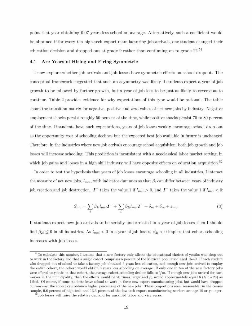
point that year obtaining 0.07 years less school on average. Alternatively, such a coefficient would

be obtained if for every ten high-tech export manufacturing job arrivals, one student changed their

education decision and dropped out at grade 9 rather than continuing on to grade 12.51

4.1 Are Years of Hiring and Firing Symmetric

I now explore whether job arrivals and job losses have symmetric effects on school dropout. The

conceptual framework suggested that such an asymmetry was likely if students expect a year of job

growth to be followed by further growth, but a year of job loss to be just as likely to reverse as to

continue. Table 2 provides evidence for why expectations of this type would be rational. The table

shows the transition matrix for negative, positive and zero values of net new jobs by industry. Negative

employment shocks persist roughly 50 percent of the time, while positive shocks persist 70 to 80 percent

of the time. If students have such expectations, years of job losses weakly encourage school drop out

as the opportunity cost of schooling declines but the expected best job available in future is unchanged.

Therefore, in the industries where new job arrivals encourage school acquisition, both job growth and job

losses will increase schooling. This prediction is inconsistent with a neoclassical labor market setting, in

which job gains and losses in a high skill industry will have opposite effects on education acquisition.52

In order to test the hypothesis that years of job losses encourage schooling in all industries, I interact

the measure of net new jobs, lmci, with indicator dummies so that βi can differ between years of industry

job creation and job destruction. I+ takes the value 1 if lmci > 0, and I− takes the value 1 if lmci < 0:

Smc =∑i

β1ilmciI+ +

∑i

β2ilmciI− + δm + δrc + εmc. (3)

If students expect new job arrivals to be serially uncorrelated in a year of job losses then I should

find β2i ≤ 0 in all industries. As lmci < 0 in a year of job losses, β2i < 0 implies that cohort schooling

increases with job losses.

51To calculate this number, I assume that a new factory only affects the educational choices of youths who drop outto work in the factory and that a single cohort comprises 5 percent of the Mexican population aged 15-49. If each studentwho dropped out of school to take a factory job obtained 3 years less education, and enough new jobs arrived to employthe entire cohort, the cohort would obtain 3 years less schooling on average. If only one in ten of the new factory jobswere offered to youths in that cohort, the average cohort schooling decline falls to 3/10. If enough new jobs arrived for eachworker in the municipality, then the effects would be 20 times larger and βi would approximately equal 6 (3/10 ∗ 20) asI find. Of course, if some students leave school to work in these new export manufacturing jobs, but would have droppedout anyway, the cohort can obtain a higher percentage of the new jobs. These proportions seem reasonable: in the censussample, 9.6 percent of high-tech and 13.3 percent of the low-tech export manufacturing workers are age 18 or younger.

52Job losses will raise the relative demand for unskilled labor and vice versa.

19

Table 4 shows the results of regression 3. The positive net new jobs per worker coefficients are

very similar to the coefficients on net new jobs per worker in table 3. Now, however, the positive

coefficient on new job arrivals in non export manufacturing is significant. The hypothesis of asymmetric

expectations is supported. While years of job growth have mixed effects on education across industries,

years of job decline increase schooling in all industries. In the two industries where I find significant

positive schooling effects for positive net new jobs, the impacts of positive and negative job arrivals

are significantly different at the 1 percent significance level (β2i < β1i).

Therefore, the assymetric educational impacts of years of job growth and decline provides evidence

in support of a conceptual framework that incorporates stochastic vacancies. In subsequent sections

of the paper, I will focus on the positive net new job effects that describe the educational impacts

of a successful export-oriented industrialization policy.

4.2 Direct and Indirect Employment Channels

I now explore the mechanisms through which new job arrivals are affecting educational decisions.

Most obviously, a youth may change his or her schooling decision in anticipation of employment at

one of the formal sector firms in my sample. First, I will investigate the effects of new job arrivals

at additional ages of exposure and over specific time periods, before addressing the possibility that

more indirect mechanisms are at play.

Up until this point, I have included only a single age of exposure in my specification, and looked

at new job arrivals at ages 15 and 16. This age was chosen as it is both the modal school leaving

age in Mexico and the age of first legal employment in formal manufacturing. However, jobs arriving

at other ages may also affect educational choices. Accordingly, I modify equation 3 to include the

new job arrivals, lmci, for cohort c at every age between 13/14 and 17/18.53 Of course including even

4 additional lags comes at a substantial cost, as the panel length contracts from 13 to 9 years and

estimates are less precise. The resulting IV regression coefficients are shown in table 5. The estimates

for positive net new job arrivals are plotted in figure 6 for years of schooling, as well as an alternative

dependent variable, the average grade 9 dropout rate for the cohort.54

53The specification is Smc =∑

i

β1ilmi13/14I+ + ...+∑

i

β1ilmi17/18I+ + ...+ δm + δrc + εmc.54The grade 9 dropout rate is calculated as the number of students who obtain only 9 years of school divided by

the number of students who obtain 9 or more years of school. In figure 6 the coefficients are inverted in order to mirrorthe total years of schooling panel.

20

The multiple year of exposure estimates in the upper panel provide supportive evidence that my

estimates are the result of students evaluating the opportunity cost of and return to school, and not

trends or third factors. There are generally negative, or less positive, schooling impacts when new job

arrivals occur at common school leaving ages (13/14 after primary school, 15/16 at the end of secondary

school and 17/18 at the end of high school). In contrast, in the in between school level ages of 14/15

and 16/17, there are positive schooling impacts of new jobs in all industries. At these school stages, the

return to one additional year of education is relatively high, since the student may be able to graduate

from secondary or high school and benefit from the sheepskin effect. The dip in years of schooling

is largest at ages 15/16, when formal sector employment is first possible in most workplaces and the

opportunity cost of schooling is particularly high. The effects of new export job arrivals at ages 13/14

on total schooling may in part be coming from youths dropping out of school at grade 7 as they expect

to obtain a factory job in the future without the need for additional education. The lower panel showing

grade 9 dropout corroborates these results, with the only significant increase in grade 9 dropout in

coming with new high-tech export manufacturing job at ages 15/16, and not at older or younger ages.55

The estimates from the multiple exposure age regression can be used to verify that my results

produce reasonable estimates of the total educational impact of new job arrivals. I multiply the

coefficients in table 5 by the actual employment shocks that occurred in Mexico when the cohorts

aged 18-26 in the year 2000 were growing up. The estimates suggest that had no new jobs arrived

in either export industry over the period, these cohorts would have acquired 0.048 years less education

on average. This reduction in schooling would be the result of 165,000 students forgoing exactly three

year education—secondary or high school for example—in order to take a new export job. In the

year 2000 census, 532,000 members of my sample aged 18-26 were employed in the export sectors.

The estimates seem reasonable, and would match the census data if 367,000 students chose to work

in the export sector without altering their education decision.56

Looking at later exposure ages can serve as a placebo test. If my results are driven, as I claim, by

students altering education decisions when new job opportunities arrive in their municipality, then new

job arrivals should not affect education levels if they arrive after all education decisions are complete.

55There are significant reductions in school dropout when new jobs arrive in professional services at ages 14/15 and16/17, as well as high-tech export manufacturing at ages 14/15. Note that new job arrivals that induce students to stay onat school will reduce school dropout at later ages if students decide to complete more than one additional year of school.

56Of course, some students may forgo more or less than three years of school, and some workers may have changedsectors between leaving school and the year 2000.

21

Net new job arrivals are highly correlated over time, and so separately estimating equation 3 for

multiple exposure ages will not provide an accurate representation of coefficient on nearby ages of

exposure. However it does allow many more ages of exposure than simultaneously including multiple

exposure ages. The lower panel of figure 6 presents the IV coefficients on positive net new jobs per

worker arriving at every age of exposure between 7-8 and 23-24. The placebo test is satisfied, as there

are no educational impacts from new manufacturing jobs by ages 22-23, the age at which students

graduate college and education decisions are complete.57

Finally, as one further check, I look at the decision to partake in technical versus general education.

In Mexico, the technical track in secondary and high school offers less academically able students

the opportunity to obtain technical training. These students are most likely to go into professional

and technical services, with 37.5 percent of high school educated students in this sector in possesion of

a technical education.58 Column 4 of table 6 shows that when new export jobs arrive, the proportion

of students taking the technical track shrinks, presumably as these less academically minded students

are the most likely to want to work in a factory. In contrast, when new professional and technical

service jobs arrive, the proportion of students choosing the technical education track rises. Table 6 also

shows school dropout regressions at grade 7, 10 and 12, with the estimates suggesting that commerce

and low-tech export manufacturing affect low education types, and non export manufacturing affects

higher education types, with professional services and non-export manufacturing in between.59

A substantial literature, cited extensively in the introduction, has shown that the returns to education

in Mexico changed over the sample period. The lower panel of figure 7 shows this evolution using

the National Urban Employment Survey. The returns to high school rose through 1993 and then by

2000 had fallen back to their 1988 level.60 By breaking my 1986-1999 sample into five-year rolling

subsamples, I can loosly evaluate the evolution of the schooling impacts over time. The coefficients

for each of these subsamples are plotted in the upper panel of figure 7. Reassuringly, the schooling

57The only impacts at ages 22-23 come from the two service industries. In table ??, I show that these effects aredriven by the least educated groups. There is evidence of adult education in the 2000 census. Over 600,000 peopleolder than 20 report currently attending school, yet have not completed grade 12. Therefore, the least skilled maycontinue to acquire skills in response to new service sector jobs at older ages.

58This falls to just under 30 percent in all four other sectors.59While all export manufacturing and service sectors have effects at grade 7, only professional services and high-tech

export manufacturing continue to have effects at grade 10. The coefficient on non export manufacturing is at its largestfor grade 12 dropout, although the standrad errors are also large as the sample of students reaching this level is small.

60The returns to college also rose until 1994, before flattening out, while the returns to lower levels of educationremained essentially flat over the period.

22

effects of new jobs in all industries approximately follow this inverted U pattern as well, with school

dropout largest at the tail end of the sample period, when returns to high school were actually falling.61

Therefore, looking across subperiods provides further evidence that new job arrivals alter educational

choices by changing the trade off between the opportunity cost of, and the returns to, school.

There are two other possible mechanisms through which new job arrivals are affecting educational

decisions. New formal sector jobs may create additional informal sector jobs which youths are attracted

to, for example informal piece-work contracts for a formal manufacturing firm. My methodology

will not be able to discriminate between direct and indirect employment of this type, as no data is

available on annual informal sector employment. However, this mechanism has very similar policy

implications to the direct employment channel and so this may not be a major worry.

Conversely, new export manufacturing plants may create additional formal sector jobs that provide

services to these plants. By including new job creation in services as a separate variable, any spillovers

of this sort will be attributed to service job creation and not export manufacturing. Column 5 of

table 6 includes only new job creation in the three manufacturing sectors. The coefficients on new

manufacturing jobs change little, suggesting that any spillovers to service sector employment have

a minimal impact on educational choices.

The second alternative mechanism is that new job arrivals may impact another family member and

thereby change household income or necessitate youths looking after younger siblings. As education is a

normal good, job arrivals should increase household income and raise educational attainment.62 There-

fore, household income seems an unlikely explanation for the school dropout effects on new export oppor-

tunities. However, if a youth’s mother or sister enters the workforce with the arrival of new job opportuni-

ties, the youth may be required to drop out of school to look after other family members. In order to test

this hypothesis, in column 6 of table 6 I include both net new jobs per worker and net new female jobs per

female worker. If this channel is behind my results, the schooling effects should be driven by new female

job opportunities rather than total new job opportunities. The results suggest that the positive schooling

impacts of new service jobs are being driven by female job opportunities, perhaps through the income

channel, but the negative schooling coefficients are driven by general, not female specific, job creation.63

61Additionally, credit constraints raise the cost of funding additional schooling, and were more likely to bind afterthe banking collapse with the peso crisis in 1995.

62For evidence on positive schooling effects of trade liberalization through the income channel, see Edmonds andPavcnik (2005) and Edmonds, Pavcnik, and Topalova (2008).

63There is strong evidence that female earned income is more likely to be spent on human capital investments than

23

In conclusion, I find that new export manufacturing opportunities induce students to drop out

of school, while new opportunities in other industries generally encourage skill acquisition. These

differences are at first glance suprising. In particular, both high-tech export and non export manu-

facturing employ workforces with similar education levels, yet new job arrivals in the two sectors have

opposite impacts on education. In the conceptual framework, I highlighted the additional industry

characteristics beyond the skill level of the workforce that, in a world of stochastic vacancies, can drive

such heterogenous responses. In section 6, I show that the variation in these characteristics across the

different industries can explain my findings. However, first, I explore the robustness of these results.

5 Robustness Checks

I perform a variety of robustness checks to ensure that my findings are not spurious. Tables 7 and 8

rerun the preferred IV specification, shown in column 1, with several modifications. Column 2 includes

a municipality-level linear time trend. This trend controls for omitted variables that trend up or down

relative to other municipalities in the state. As the peso crisis occurred in the middle of the sample, a

linear trend may be misleading. Additionally, with only 13 years of data, even including a linear trend

terms risks over-fitting and causing attenuation due to the inclusion of an excessive number of controls

in the regression. However, the coefficient on high-tech export manufacturing remains significantly

negative, although smaller than in the basic specification.64 In column 3, I cap education at 12 years and

recalculate cohort schooling. By capping education at 12 years, most of the sample will have reached

their final level of schooling by the year 2000, mitigating concerns that the amount of misreporting

varies with the skill level of the municipality. In column 4, I further restrict attention only to individuals

not at school at the time of the census. Results are very similar in both cases, therefore, I can be

confident that my results are driven by students making school dropout decisions before the end of high

school. Columns 5 and 6 split the sample into men and women.65 I find similar results for both sexes.

Column 7 shows that my results are robust to extending the cutoff threshold of my instrument from

changes of 50 employees to changes of 100 employees in a single firm. Column 8 excludes the 781 small

male earned income, e.g. Duflo (2003).64The other two manufacturing coefficients retain their signs and fall slightly but are no longer significant. The

two coefficients on services actually reverse sign. The service sector is the most likely sector to suffer from reversecausation as fixed costs of expansion are smallest in this sector where less capital equipment is needed.

65The new jobs variables are net new (fe)male jobs per (fe)male worker and I instrument with net new (fe)malejobs per (fe)male worker for firms experiencing large expansions or contractions in total employment.

24

municipalities that saw no formal sector job growth over the period.66 The coefficient on low-tech export

manufacturing is no longer significant when these comparison municipalities are removed. Column 9

includes controls that account for the fact that rural municipalities may have seen differential trends over

time and that the Progresa conditional cash transfer program was rolled out at the end of the period.67

Further robustness tests are shown in table 8. Column 10 excludes the two large cities in the sample,

Monterrey and Guadalajara, which may have been driving my population weighted results. In both

cases, results are unchanged. Columns 11 includes the Valle de México metropolitan zone contains

Mexico City. As this city forms its own state, I remove the state-time dummies and replace then

with region-time dummies for six broad regions. Columns 12 and 13 look at differences between

metropolitan and non-metropolitan municipalities. Again, I use region-time dummies for both these

regressions as there are only 54 metropolitan zones in my data set and so including state-time dummies

for each of the 31 states would remove any interesting variation across cities. The results suggest

that the low tech export manufacturing and commerce effects found in the main specification are

coming primarily from non-metropolitan municipalities.

I also explore how the results vary over different regions of Mexico. In columns 14 through 16, I

divide the municipalities into three regions. In columns 17 through 20, I split the municipalities by

both average education and average income in the year 2000. There is a positive effect on education

from new high-tech export manufacturing jobs in the south, and the least educated areas of the country,

where very few such jobs were created. These results suggests that the initial skill distribution of the

municipality matters, as high-tech export manufacturing jobs demand relatively high skills compared

to average schooling levels in these areas. Poorer and less educated municipalities experience relatively

larger negative education effects from low-tech export manufacturing.68 In summary, there is a robust

negative impact of new job arrivals in export manufacturing on educational attainment.

66For 67 percent of periods in my sample there was no change in formal sector employment. However, as thesezeroes generally occur in small municipalities, they have little impact on my weighted regression results.

67To control for rural trends, I include a full set of state dummies interacted with a time trend multiplied by the percent-age of the municipality population that is classified as rural. Progresa could potentially be a cause of omitted variable bias asthe program encouraged children to stay in school at the tail end of my sample period by offering cash incentives. Therefore,I also include a Progresa dummy takes the value 1 in the 1998 and 1999 if more than 10 percent of the population reportedreceiving Progresa or Procampo payments in the 2000 census (no specific Progresa indicator is available in the census)

68A possible explanation for this finding is that families in poorer municipalities are less able to financially support youthsstill at school (low yt), and so dropout is relatively more tempting when very low skill jobs arrive in these municipalities

25

5.1 Migrants, Non-Migrants and Selective Migration

My results only pertain to the population of non-migrants. As the census does not record where

migrants were living at ages 15 and 16, I cannot match these individuals to new local job opportunities

at these ages and so I exclude them from my sample. Many export manufacturing workers migrate

from poorer, often rural areas. McKenzie and Rapoport (2006) find that the option to migrate to

the United States lowers educational attainment in Mexico.69 Therefore, a plausible hypothesis is

that my results understate the true educational decline as some potential migrants drop out of school

in the belief that the benefits of migration have risen with the arrival of export manufacturing jobs

in other municipalities. Unfortunately, I cannot examine this hypothesis using my empirical strategy.

However, migration effects could still bias my results if local labor market conditions differentially

affect out-migration by skill group. For example, a new factory may stop a low skill worker from

migrating, but have no impact on the migration decision of a high skill worker. The cohort average

education, measured in the year 2000, could then fall, but the cause is the reduced out-migration of low

skill workers. In appendix A, I address the concern that the negative schooling coefficients I find originate

from such compositional effects. First, I show that new export manufacturing jobs do not affect the

sample cohort size. Second, I use census data on the municipality of residence in 1995 to show that when

new jobs arrive, it is the more skilled who are less likely to migrate. This finding only applies to internal

migrants, but Chiquiar and Hanson (2005) find similar effects for emigrants to the United States.70

Therefore, the negative impacts of export manufacturing that I find are likely even larger in magnitude,

because compositional effects bias the coefficient upwards and attenuate my estimated coefficient.

Migration may also bias results in other ways. If rural youth are more likely than urban youth to

migrate in search of jobs or to attend secondary school, then rural youths will be underrepresented in

my sample. As three quarters of Mexicans live and most formal sector jobs are found in urban areas,

this underrepresentation is likely to only have a small impact on my population-weighted estimates,

however there is still reason to be cautious. Alternatively, large exogenous flows of migrants into a

municipality may alter both education and factory location decisions. However, omitting migrant flows

from my specification would likely exert an upward bias on my estimates. An increase in low-skill

migrant labor should lower the local unskilled wage, attracting factories and encouraging local students

69Similarly, de Brauw and Giles (2008) show that, for rural China, reduced migration costs increase school dropout.70However, in a recent paper, Moraga (2008) disputes this finding for international migrants.

26

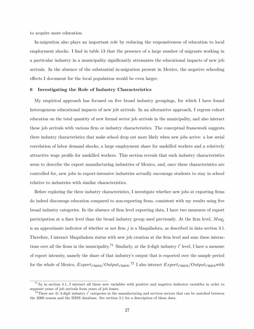
to acquire more education.

In-migration also plays an important role by reducing the responsiveness of education to local

employment shocks. I find in table 13 that the presence of a large number of migrants working in

a particular industry in a municipality significantly attenuates the educational impacts of new job

arrivals. In the absence of the substantial in-migration present in Mexico, the negative schooling

effects I document for the local population would be even larger.

6 Investigating the Role of Industry Characteristics

My empirical approach has focused on five broad industry groupings, for which I have found

heterogenous educational impacts of new job arrivals. In an alternative approach, I regress cohort

education on the total quantity of new formal sector job arrivals in the municipality, and also interact

these job arrivals with various firm or industry characteristics. The conceptual framework suggests

three industry characteristics that make school drop out more likely when new jobs arrive: a low serial

correlation of labor demand shocks, a large employment share for unskilled workers and a relatively

attractive wage profile for unskilled workers. This section reveals that such industry characteristics

seem to describe the export manufacturing industries of Mexico, and, once these characteristics are

controlled for, new jobs in export-intensive industries actually encourage students to stay in school

relative to industries with similar characteristics.

Before exploring the three industry characteristics, I investigate whether new jobs at exporting firms

do indeed discourage education compared to non-exporting firms, consistent with my results using five

broad industry categories. In the absence of firm level exporting data, I have two measures of export

participation at a finer level than the broad industry group used previously. At the firm level, Maqj

is an approximate indicator of whether or not firm j is a Maquiladora, as described in data section 3.1.

Therefore, I interact Maquiladora status with new job creation at the firm level and sum these interac-

tions over all the firms in the municipality.71 Similarly, at the 3-digit industry i′ level, I have a measure

of export intensity, namely the share of that industry’s output that is exported over the sample period

for the whole of Mexico, Exporti′mex/Outputi′mex.72 I also interact Exporti′mex/Outputi′mexwith

71As in section 4.1, I interact all these new variables with positive and negative indicator variables in order toseparate years of job arrivals from years of job losses.

72There are 41 3-digit industry i′ categories in the manufacturing and services sectors that can be matched betweenthe 2000 census and the IMSS database. See section 3.1 for a description of these data.

27

new job arrivals, but here by 3-digit industry, and sum these terms over all industries i′:

Smc = β1I+ ∑j∈m

lmcj + β2I+ ∑j∈m

lmcjMaqj + β3I+ ∑i′

lmci′Exporti′mexOutputi′mex

+ ...+ δm + δrc + εmc. (4)

My previous findings suggest that new job arrivals at Maquiladora firms or in sectors with high export

intensities will discourage education compared to other jobs; β2 < 0, β3 < 0.

Table 9 reports the results of this regression. Columns 1 and 2 include only one of the two exporter

interactions and column 3 contains both terms. As expected, the coefficients β2 and β3 are negative.

New job arrivals within Maquiladora or within industries with a high export intensity significantly

reduce educational attainment, while new job arrivals alone encourage schooling.73

In the next three subsections, I interact new job arrivals with measures of the three industry

characteristics described in the conceptual framework, and add these terms to equation 4. The results

of this regression are shown in column 4 of table 9.

6.1 Serial Correlation of Job Creation

The conceptual framework predicts that if hiring is only weakly serially correlated within an industry,

new jobs would be more likely to encourage drop out since such opportunities are less likely to also be

available the next year. The transition matrix for positive, zero and negative net new jobs in table 2

shows that the two export manufacturing sectors have the lowest probability of a positive shock being

followed by another positive shock.74 Consequently, I interact new job arrivals with the transition

probability that a year of municipality job growth in a 3-digit industry is followed by another year

of job growth.75 The predicted positive sign is found is only found once controls for industry growth

and firm size are included and is not significant. Therefore, there is no strong supportive evidence

that new export jobs induce dropout in part because the relative volatility of job growth in these

industries encourages students to grab jobs when they become available.

73When both are included, the Maquiladora term remains negative but becomes insignificant. Maquiladoras arehighly concentrated in export-intensive industries, and so the fact that one of these two exporting interaction termsbecomes insignificant is not surprising.

74I also estimate an Arellano-Bond linear dynamic panel estimator and find a negative coefficient on past job growthonly for high-tech export manufacturing. However, the panel is too short to differentiate the autoregressive processesacross the different industries.

75These probabilities are calculated from the IMSS dataset. For the negative net new jobs terms, I interact thetransition probability that a year of losses is followed by another year of losses. Ideally, I would estimate an ARMAmodel for each industry. However, the brevity of my panel precludes this.

28

6.2 Skill Level and Age of Employees

The conceptual framework suggests that new job arrivals in an industry where almost all jobs

require high education levels will not induce dropout for students with low skills, since the opportunity

cost of schooling does not change. Similarly, if an industry only employs more experienced older

workers, immediate employment is not possible for a student and the opportunity cost of school will

not rise with new job arrivals.

Figure 3 uses the 2000 census to show histograms of years of schooling and age for my five broad

industry categories, as well as for the residual informal sector.76 Low-tech export manufacturing

demands the least skilled workers of the formal sector industries, with 40 percent the workforce having

less than 9 years of schooling. Non export manufacturing and high-tech export manufacturing have

almost identical skill distributions.77 The service sectors are more skilled and the informal sector is,

unsurprisingly, the least skilled.78 The 1990 census shows similar patterns, although with workers in all

sectors having relatively less education. In terms of the age distribution of employees, shown in figure 4,

both export manufacturing sectors have significantly younger workforces. The younger age distribution

may be a result of faster growing firms in these industries. I therefore exclude this variable, or add

an additional control explicitly for firm growth in the regression specification. In summary, the export

sectors have a comparatively young and unskilled workforce compared to other formal industries.

Guided by these descriptive statistics, I include two interaction terms calculated at the 3-digit

industry from the 2000 census in equation 4. The results are shown in columns 4 and 5 of table

9, while column 6 shows the same interaction terms but using the 1990 census.79 To measure the

abundance of jobs available for unskilled workers, I interact new job arrivals with the national share

of workers in industry i′ with less than a high school diploma, S < 12. To measure the abundance

of jobs available for young workers straight out of school, I interact new job arrivals with the national

76I define private formal sector workers in the census as full-time workers with IMSS health insurance and non-zeroincome. Wives, children and unemployed husbands of IMSS workers are also eligible for IMSS insurance, and mayimpart some error. To match the sample of my main specification, the skill level sample comprises non-migrants aged16 to 28. The age sample comprises non-migrants aged 15-50.

77Therefore, the skill level of the industry is not able to explain my finding that new jobs arrivals in these twoindustries had opposite effects on schooling. In a neoclassical labor market framework, this characteristic would determinewhether or not new jobs in an industry encouraged school dropout.

78There are some excluded formal sector workers in this group: public sector employees insured by ISSSTE, employeesof PEMEX and a relatively small number of agriculture, construction, mining and utilities workers insured by IMSS.

79For 1990, as the census does not ask about IMSS status, I use the full sample of workers.

29

share of employees in industry i′ who are likely to have been in the workforce for 3 years or less.80

The higher the proportion of new jobs that are available to the young and unskilled, the more likely it

is that new job arrivals will encourage school dropout. Therefore, the coefficients on these interaction

terms should be negative. I find support for these conjectures, with significant negative coefficients on

the skill level interaction terms in all specifications and the age term when using the 1990 census data.

6.3 Wages Paid at Different Skill Levels

The conceptual framework suggests that the attractiveness of industry wages at different skill levels

affects the dropout decision. New jobs in the industry are more likely to induce drop out if the wages

for unskilled workers, relative to other industries, are high in comparison to the wages for skilled

workers, again relative to other industries.81

The relative wages paid by different broad industry categories can be seen most clearly in figure

8. This figure shows plots of the wage differences between each industry and the local informal sector

by skill level from the 2000 census for new workers in their first years of employment.82 These premia

should be treated with some caution as they do not take account of workers sorting on unobservables.

However, they still provide useful evidence on wage differences by skill and industry. For workers with

only 6 years of school, low-tech export manufacturing offers high premia of over 17 percent and this

premia declines rapidly at higher levels of education. For intermediate years of schooling, high-tech

export manufacturing offers high premia of about 15. However, with 12 years of schooling, non export

manufacturing offers the best premia of about 14 percent over the informal wage for that level of

schooling, while the export sectors offer significantly smaller premia of between 5 and 9 percent.83 The

within industry returns to education and the wage profiles in figure 9 show similar patterns in the 6-12

80I assume workers graduated in the expected year based on their age, and calculate likely experience as age minusschooling minus 6. If a worker has less than 9 years of education, I count the number of years since they turned 16,the legal factory employment age.

81If this ratio is high, a new job opportunity is more likely to affect the best job today than it is to affect the expectedbest future job.

82I focus on 6 to 12 years of schooling, the relevant education margin for most manufacturing workers inMexico. These are wages for workers with five or less years of experience (age minus schooling minus six) postage 16. To estimate these wage premia, I run a Mincer-like wage regression of log income for individual j on aset of industry-school level dummies, dids. I also include a full set of municipality-school level fixed effects, γms:lnYjmis =

∑i 6=informal

∑sψisdids +

∑m

∑sγmsdmds + Xj + εjmis. By omitting the schooling dummies for the

informal sector, the coefficients ψis on the other industry dummies measure the premium that each industry i paysover the informal sector wage at that skill level s. Controls, Xj , include sex, experience and a rural dummy. To obtainestimates of wage premia that are representative of the non-migrant population of Mexico excluding Mexico City, Iweight wages in each municipality by the regression municipality weights.

83The wage premia for high-tech export manufacturing and non export manufacturing are significantly differentat both 9 and 12 years of schooling.

30

years of schooling range, with a significantly lower return to high school in the export industries.84

These descriptive statistics are consistent with the very different schooling impacts of new jobs

across the three manufacturing industries detailed in section 4. The premia in the two export sectors

are most generous at lower skill levels, while the premia in non export manufacturing remain generous

for high school graduates. Accordingly, we would expect new low-tech export manufacturing jobs

to have the largest effects on youths with less than secondary school, high tech export manufacturing

to induce students to leave school after grade 9, and non export manufacturing jobs to potentially

entice students to stay and complete high school.

These high premia in the export sectors support the ample evidence that exporters and foreign

firms in Mexico pay high wages for a given skill level (e.g. Bernard 1995). For the relatively low skilled

workers they employ (75 percent of employees with 9 years of education or less), export manufacturing

jobs are highly remunerated compared to jobs in other sectors.

The insights that come from the census wage figures can be tested more rigorously by including

an interaction term suggested by the conceptual framework : the ratio of the wage differences over

the informal sector at 9 and 12 years of schooling in industry i′, again from either the 2000 or 1990

census.85 I should find a negative coefficient on this interaction term if new job arrivals are more

likely to induce drop out when they offer relatively more attractive wages to low skill rather than high

skill workers, compared to other local opportunities at those skill levels. The conjecture is supported

by significant negative coefficients on the interaction term in columns 4, 5 and 6 in table 9.

6.4 Exporting, Industry Characteristics and Dropout

Finally, I include two additional firm-level controls to equation 4 in columns 5 and 6. First, I interact

firm size (in terms of employees) with firm-level changes in employment. Firm size is a standard firm

characteristic in the trade literature, but it is only weakly significant in this context. Second, I interact

national industry average growth rates. The interaction terms suggested by the conceptual framework

are likely to be correlated with industry growth rates (for example, the age of the workforce). I

84For the returns to education, I run Mincer-like regressions again for new workers, but now including municipality-industry fixed effects instead of municipality-school level ones. I omit all the industry-school level dummies for workers with9 years of education, and obtain the returns relative to 9 years of schooling in that industry for non-migrants in Mexicoexcluding Mexico City. For wage profiles, I plot locally weighted regressions of the wage relative to the local informal sectorwith 9 years of school to allow comparability across education levels and industries. I restrict the sample to men sincemany women in Mexico drop out of the labor market and return in later life, breaking the link between age and experience.

85As the 1990 census does not record IMSS membership, I use the wage differences over the local domestic serviceindustry.

31

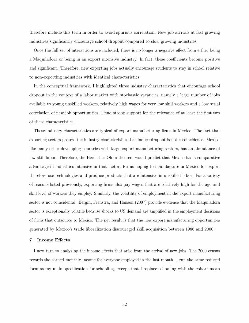
therefore include this term in order to avoid spurious correlation. New job arrivals at fast growing

industries significantly encourage school dropout compared to slow growing industries.

Once the full set of interactions are included, there is no longer a negative effect from either being

a Maquiladora or being in an export intensive industry. In fact, these coefficients become positive

and significant. Therefore, new exporting jobs actually encourage students to stay in school relative

to non-exporting industries with identical characteristics.

In the conceptual framework, I highlighted three industry characteristics that encourage school

dropout in the context of a labor market with stochastic vacancies, namely a large number of jobs

available to young unskilled workers, relatively high wages for very low skill workers and a low serial

correlation of new job opportunities. I find strong support for the relevance of at least the first two

of these characteristics.

These industry characteristics are typical of export manufacturing firms in Mexico. The fact that

exporting sectors possess the industry characteristics that induce dropout is not a coincidence. Mexico,

like many other developing countries with large export manufacturing sectors, has an abundance of

low skill labor. Therefore, the Heckscher-Ohlin theorem would predict that Mexico has a comparative

advantage in industries intensive in that factor. Firms hoping to manufacture in Mexico for export

therefore use technologies and produce products that are intensive in unskilled labor. For a variety

of reasons listed previously, exporting firms also pay wages that are relatively high for the age and

skill level of workers they employ. Similarly, the volatility of employment in the export manufacturing

sector is not coincidental. Bergin, Feenstra, and Hanson (2007) provide evidence that the Maquiladora

sector is exceptionally volatile because shocks to US demand are amplified in the employment decisions

of firms that outsource to Mexico. The net result is that the new export manufacturing opportunities

generated by Mexico’s trade liberalization discouraged skill acquisition between 1986 and 2000.

7 Income Effects

I now turn to analyzing the income effects that arise from the arrival of new jobs. The 2000 census

records the earned monthly income for everyone employed in the last month. I run the same reduced

form as my main specification for schooling, except that I replace schooling with the cohort mean

32

of log earned income, lnYmc for employed workers:86

lnYmc =∑i

β1ilmciI+ +

∑i

β2ilmciI− + δm + δrc + εmc. (5)

The identification argument and the IV strategy are identical to those detailed for the schooling

regression in section 3.3. However, reverse causality is less of an issue than in the schooling case as it

is unlikely that cohort income deviations in the year 2000 influenced labor demand in previous years.

The income effects of net new job arrivals generally mirror the educational impacts and are shown

in table 10. Those industries where new jobs encourage more schooling see positive income gains, as

would be expected. However, for high-tech export manufacturing, where new jobs discourage education

acquisition, I find the opposite effects. Despite the high wages on offer in the industry, by the year 2000

the average log income of cohorts heavily exposed to the arrival of high-tech export manufacturing

jobs in earlier years actually declines compared to less exposed cohorts.87 The arrival of low-tech

export manufacturing jobs brings no such income losses in later years.88

The results above pertain only to employed workers. Column 4 of table 11 shows the results

of replacing lnYmc in equation 5 with the cohort labor force participation rate for individuals not

reporting still being at school. The negative income effects of high-tech export manufacturing described

above would have a different interpretation if labor force participation rose. However, labor force

participation in the year 2000 actually fell with new job opportunities at ages 15 and 16 in this

industry, consistent with the high rates of volatility and churn in this industry.

Additionally these estimates, along with the income estimates above, are broken down by gender

in the other columns of table 11. There are no gender differences in the impacts of high-tech export

jobs. However, female labor force participation does rise significantly when new low-tech export and

professional service jobs arrive for females, effects not found in the male sample.

The magnitude of the income loss from high-tech export manufacturing conforms with the estimates86This measure excludes everyone who reports no earned income, and so I am evaluating the wage margin not the

labor market participation margin. I use log income as is standard in the labor literature, both to reduce problems relatedto outliers and because income is typically log normal. I drop all workers who report working for less than 20 hours perweek, and winsorize the log wage at the 1 percent tails. Results are essentially unchanged without this cleaning procedure.

87There is no evidence that new jobs in export manufacturing alter the variance of earned income, perhapscompensating for the lower income. A similar specification to equation 5, but with log income replaced by the varianceof log income, produces insignificant coefficients.

88One possible explanation for the lack of a negative income effect, despite lower schooling, is that new jobs atthese firms induce the very lowest skill groups to drop out. For this group, the returns to education are particularlyflat, and these firms pay a very high premium over the informal sector (shown in figures 9 and 8).

33

of the returns to schooling in Mexico. For my preferred IV specification, I find a negative coefficient

of -0.580 on log income. This corresponds to a “return to schooling” of 7.9 percent per year.89 This

return to an additional year of schooling is in the range of between 7.5 percent and 16.1 percent

suggested by Patrinos (1995) and Psacharopoulos, Velez, Panagides, and Yang (1996) for Mexico. An

estimate of the returns to schooling in the lower end of this range is not surprising, given that these

are hypothetical returns to schooling. I am comparing the income of a student for whom new export

manufacturing plants open at her key school leaving age to the income of an otherwise identical student

in the alternative scenario, where no factory opened. Because these new export jobs pay high wages,

the estimated returns to schooling will be lower than the genuine returns to schooling for the student

in the alternative scenario, who did not have a new high-paying export manufacturing job on offer.

I can also calculate a back of the envelope discount rate using my conceptual framework and the

coefficients on new high-tech export jobs. With a constant wage throughout the workers lifetime and

at-school income at half of work income, the value of the implied discount rate is 11 percent with

log utility (where coefficient of risk aversion, σ, equals 1).90

It is valuable to note that these coefficients are not representative of the population as a whole. My es-

timates derive from comparing the subset of the population whose educational choices and incomes were

altered by the arrival of new factories in their municipality to similar subgroups who were not exposed

to the arrival of new factories at key school leaving ages. This subgroup likely contains youths who have

unusually high returns from, or a particular disposition for, factory work. The impact of new factory

jobs on the subgroup of non-migrants whose decisions are altered by large firm expansions or contrac-

tions is particularly relevant. For an industrial policymaker considering how the education of the local

population is affected by the placement of a new factory, this is a subgroup that is of primary interest.

7.1 Individual Welfare Implications

The large positive externalities associated with education make government intervention justifiable.

However, before addressing such policy considerations in the conclusion, I will focus on the welfare

implications of my findings for the individuals making the education decisions.

In light of my findings, it is important to note that incomes losses do not imply welfare losses. Some

89The returns to schooling is the exponential of the income coefficient divided by the coefficient on schooling.90For σ=0.5 the discount rate rises to 13.3 percent, and falls to 7.3 percent for σ=2. If at-school income is a quarter

of work income, the discount rates are 2.4 percent, 5.5 percent and 7.6 percent in order of descending risk aversion.

34

impatient, risk averse or credit-constrained students will quite rationally forgo schooling for immediate

income gains, knowing that in a few years their salaries may be lower than if they had stayed at school.

Policymakers could still have paternalistic concerns for their citizens if they believe that adolescents are

particularly predisposed to discount the future heavily when faced with delayed and uncertain gains.91

Similarly, peer effects at this stage of life are particularly strong, and may cause excessive dropout rates.92

Credit constraints can also result in youths dropping out of school when new jobs arrive if there

are high-return investment opportunities, such as starting a small business, that become feasible with

the income from an export manufacturing job. Atkin (2008) provides evidence for a related story,

as women induced to work in a factory at young ages make larger health investments in their children.

In order for credit constraints to explain my income findings, the returns on the investment must not

show up in earned income by the year 2000. Additionally, these credit constraints will also bind when

non-export jobs arrive for example, and so new jobs arriving in this sector would have to be impacting

educational choices of a different subpopulation that was not credit constrained. As an empirical

check on the validity of the credit constraints hypothesis, columns 4 and 5 of table 10 show that the

negative schooling coefficients are actually smaller in poorer municipalities where credit constraints

are presumably more binding.93,94 Therefore, the credit constraints story is an unlikely explanation

for the negative income effects of new jobs in high-tech export manufacturing.

In a similar vein, high-tech export firms may offer on-the-job training which is more useful to

workers than additional years of schooling. Again, the benefits to firm training must be delayed, or

else earned income would not be lower in the year 2000. While plausible, the evidence from Mincerian

wage regressions using the 2000 census suggests that the return to experience are significantly smaller

than the returns to education in both of the two export industries.95

91There is a growing body of evidence in cognitive neuroscience, discussed by Oreopoulos (2007), that adolescentsare particularly predisposed to such behavior as the frontal lobes associated with planning and decision making onlyfully develop in adulthood. For example see Sowell, Thompson, Holmes, Jernigan, and Toga (1999) or Galvan, Hare,Parra, Penn, Voss, Glover, and Casey (2006).

92In support of such hypotheses, 74 percent of American school dropouts surveyed by Bridgeland, DiIulio, andMorison (2006) would want to stay in school if they could relive that decision.

93High-tech export manufacturing increases incomes in poorer municipalities, although students still drop out ofschool early (table 8). In these areas, the high wages on offer may compensate for the lower level of education, giventhe paucity of well-paying local alternatives.

94If there are also higher returns to investment in richer municipalities, credit constraints could drive larger negativeincome effects in richer municipalities.

95I run the Mincer regression described in footnote 84 but allowing returns to experience to vary by industry. Thecoefficients on experience are 3 percent per year for both export industries, while the returns to the three years requiredto complete high school are 19 percent in both industries. Three years of export experience increases income significantlyless than attending high school.

35

There are several situations where the income losses I find would imply clear welfare losses. Students

may drop out early in anticipation of obtaining a high-tech export manufacturing job in the future,

but they are unable to obtain a job at that firm when they apply. Alternatively, students may actually

be misestimating the industry wage profile and did not expect their incomes to be lower by the year

2000.96 If students incorrectly forecast future incomes, as in these two situations, a specific policy

remedy may be appropriate if the policymaker possesses better information than the students. 97

8 Conclusions

This paper finds that for Mexico during the period 1986 to 2000, the changing industry compo-

sition brought about by trade liberalization altered the skill distribution. In particular, new export

manufacturing jobs induced students to drop out of school at younger ages. The magnitudes I find

suggest that for every ten new jobs created in high-tech export manufacturing, one student dropped

out at grade 9 rather than continuing on through grade 12. Despite high-tech export manufacturing

paying high wages for a given skill level, new jobs in this industry eventually reduced incomes for

those cohorts in school at the time these jobs arrived, since these workers acquired less education

than they would have otherwise. The specific characteristics of export manufacturing in Mexico can

explain these negative schooling impacts. Export manufacturing firms offer an abundance of jobs to

unskilled workers, these jobs are particularly volatile, and the formal-sector wages that these firms pay

are particularly remunerative at lower skill levels, all of which raised the opportunity cost of schooling.

My findings are relevant for designing industrial policies that will allow developing countries to

gain fully from the increasing globalization of production. Individual educational decisions have

positive externalities, which justify governments all over the world subsidizing school attendance.98

Accordingly, many developing countries, including Mexico, have prioritized raising the skill level of the

workforce. These policies are often based on the explicit assumption that a more educated workforce

will attract firms that produce high value-added exports, rather than simple Maquiladora-type assembly

operations. It is crucial for the success of such policies to know which types of formal sector employment

96In an earlier version of this paper, Atkin (2009) provides empirical evidence that students may not have fullyanticipated the decline in the returns to experience that new assembly line technologies brought to this industry.

97Jensen (2010) and Nguyen (2007) carry out successful information interventions that provide students with moreaccurate estimates of the returns to education. In a similar vein, emerging low-cost export manufacturing locationscould inform the local population of the volatile nature of these jobs and their likely wage profiles.

98The most prominent of these spillovers comes from educated workers making those around them more productive.Lucas (1988) suggests that such human capital externalities may be large enough to explain income differences acrossthe world, and recently Moretti (2004) provides evidence using plant-level data.

36

opportunities pull students out of school and in what context. For example, the increase in education

that accompanied new service sector opportunities in Mexico mirrors the similarly positive impacts that

the rise of information technology outsourcing has had on India. Meanwhile, the positive educational

impact of high-tech export jobs in the less-skilled south of Mexico echoes the rise in education that

accompanied Indonesia’s export driven industrialization.

Feedback loops can magnify the initial educational effects of new job arrivals. For example, if export

manufacturing lowers skill levels in a municipality, the resulting low-skill population will put downward

pressure on unskilled wages and attract even more export-assembly operations. These forces can

quickly polarize a country’s geographic distribution of schooling attainment, with skilled and unskilled

regions forming. Policymakers should also be wary that when footloose export-assembly jobs move

to lower-wage countries, as has already started happening to Mexico, the prospects for the areas that

encouraged export manufacturing could be bleak, left without jobs or skills.

Fortunately, there are several potential policy remedies. A system of payments conditional upon

school attendance would neutralize the negative educational impact of export manufacturing jobs.99

Alternatively, the age of earliest employment in export manufacturing could be raised above 16 to

ensure that most Mexican workers will have already chosen their final education levels before being

allowed to work in an export manufacturing plant. Engineering a steadier flow of new firm arrivals

could reduce dropout by putting less pressure on students to grab formal sector jobs as soon as they

appear.100 Reducing the psychic cost of returning to school in later life would allow adults to obtain

the foregone education should the export manufacturing jobs dry up or if the adult comes to regret

their decision to drop out of school. Finally, policymakers may wish to more vigorously promote the

type of exporting firms which offer jobs that demand relatively high levels of education, and thereby

encourage, rather than discourage, skill acquisition.

99The much-studied Progresa program in Mexico does just that, providing cash transfers to parents who keep theirchildren in school up to grade 9 (Schultz 2004). The roll out was too late to have an impact on my sample.

100I find some support for this hypothesis as municipalities which experienced more variable job growth had loweraverage educational attainment, conditional upon the mean job growth in the municipality. Results available on request.

37

Appendix A Migration Composition Effects

The negative educational effects of new export manufacturing jobs that I find may be spurious if

new jobs prevent low skilled individuals from migrating, and thereby lower the average education

of my sample without changing schooling decisions. I carry out two empirical tests to explore the

relevance of such out-migration composition effects.

The first test looks at the size of different cohorts of non-migrants. If these composition effects

are important, and if the less skilled are deciding not to migrate, the size of the sample cohort should

rise with new jobs in export manufacturing. To test this hypothesis, I replace cohort years of schooling

with log cohort size lnNmc in equation 2, the main specification:101

lnNmc =∑i

β1ilmciI+ +

∑i

β2ilmciI− + δm + δrc + εmc.

Table 12 shows the results from this regression. The cohort size responds positively to new service

jobs, but there seems to be no impact from new jobs arrivals in the three manufacturing sectors.

The second test examines whether skill differences between migrants and non-migrants can explain

the negative coefficients on new export manufacturing jobs. If so, I should find that the education

of out-migrants rises relative to the education of non-migrants in a municipality when new export

manufacturing jobs arrive. As the census only records where people lived in 1995, I cannot exploit

the panel dimension of my data. Instead, I take the average education of people who lived in the

municipality in 1995 but not in 2000, Sleave,mt, divided by the education of people who lived in the

municipality in both 1995 and 2000, Sstay,mt, as my dependent variable.102 The ratio is then regressed

on the sum of the changes in employment over these years by industry, interacted with positive and

negative indicator dummies. I also include a full set of state dummy variables:

15

99∑t=95

Sleave,mtSstay,mt

=∑i

β1i[99∑t=95

lmit]I+ +∑i

β2i[99∑t=95

lmit]I− + δr + εm.

If my finding of negative schooling impacts from new export jobs is driven by the less educated

remaining in the municipality when new jobs arrive, the ratio of leavers to stayers education will

101I use log cohort size as municipality populations vary greatly. By using logs I am looking at proportional changes.Net new jobs are already scaled, as they are divided by the number of workers in the municipality.

102Accordingly, I restrict my sample to cohorts who turned 15 or 16 between 1995 and 1999.

38

increase with positive changes in employment between 1995 and 2000 (β1i>0).

The results are reported in table 12. For all sectors the β1i coefficients are negative. New formal jobs

keep the more educated youth in the municipality.103 This is strong evidence, at least for the later years

in the sample, that when new jobs arrive, out-migration effects would tend to increase cohort education

averages through composition effects. Therefore, the magnitude of my finding that new export

manufacturing jobs reduce schooling is likely attenuated by out-migration. The fact that new jobs in

other sectors increased education, however, may purely or partly be coming from composition effects.

Migration may have other effects on my estmates. For example, if a particular industry only employs

migrants, then new jobs in that industry should have no impact on the education decisions of local

youth. I test this hypothesis using the in-migrants I identify in the 2000 census. I calculate ϑmi, the

proportion of migrants in each industry in each municipality and then interact ϑmi with positive and

negative net new jobs per worker:

Smc =∑i

β1ilmciI+ +

∑i

β3ilmciϑmiI+ + ...+ δm + δrc + εmc.

If the presence of migrants reduces the impact of new job arrivals on the local population, I expect

β3i to be significant and of the opposite sign to β1i. These results are detailed in table 13. For high-tech

export manufacturing, commerce and non export manufacturing, I find the expected pattern.104 The

magnitudes of β3i and β1i are similar, implying that there is essentially no effect on non-migrant

education when new jobs arrive in an industry that employs only migrants. The implication of this

finding is that, in the absence of internal migration in Mexico, local education choices will be even

more affected by the arrival of new employment opportunities than my results suggest.

103For job losses, the effects are also negative or highly insignificant, implying that the more educated leave themunicipality when there are no formal sector jobs.

104Although in the latter case, the β3i term is not significant.

39

References

Abowd, J., and T. Lemieux (1993): “The Effects of Product Market Competition on Collective Bargaining

Agreements: The Case of Foreign Competition in Canada,” The Quarterly Journal of Economics, 108(4),

983–1014.

Acemoglu, D., and J.-S. Pischke (1998): “Why Do Firms Train? Theory And Evidence,” The Quarterly

Journal of Economics, 113(1), 78–118.

Airola, C., and J. Juhn (2005): “Wage Inequality in Post-Reform Mexico,” Working Papers 2005-01,

Department of Economics, University of Houston.

Aitken, B., A. Harrison, and R. Lipsey (1996): “Wages and Foreign Ownership A Comparative Study

of Mexico, Venezuela, and the United States,” Journal of International Economics, 40(3-4), 345–371.

Akerlof, G., and J. Yellen (1990): “The Fair Wage-Effort Hypothesis and Unemployment,” The Quarterly

Journal of Economics, 105(2), 255–283.

Atkin, D. (2008): “Working for the Future: Female Factory Work and Child Health in Mexico,” Discussion

paper, Yale University.

(2009): “Endogenous Skill Acquisition and Export Manufacturing in Mexico,” Discussion Paper 224,

BREAD Working Paper Series.

Baker, G., M. Gibbs, and B. Holmstrom (1994): “The Internal Economics of the Firm: Evidence from

Personnel Data,” Quarterly Journal of Economics, 109(4), 881–919.

Baltagi, B., and C. Kao (2000): “Nonstationary Panels, Cointegration in Panels and Dynamic Panels:

A Survey,” Advances in Econometrics, 15, 7–52.

Bartik, T. (1991): Who Benefits from Dtate and Local Economic Development Policies? WE Upjohn Institute

for Employment Research Kalamazoo, MI.

Bartik, T. J. (2006): “How Do the Effects of Local Growth on Employment Rates Vary with Initial Labor

Market Conditions?,” Staff Working Papers 09-148, W.E. Upjohn Institute for Employment Research.

Beaudry, P., and J. DiNardo (1991): “The Effect of Implicit Contracts on the Movement of Wages Over

the Business Cycle: Evidence from Micro Data,” The Journal of Political Economy, 99(4), 665–688.

Becker, G. (1962): “Investment in Human Capital: A Theoretical Analysis,” The Journal of Political

Economy, 70(S5), 9.

Behrman, J. R., P. Sengupta, and P. Todd (2005): “Progressing through PROGRESA: An Impact

Assessment of a School Subsidy Experiment in Rural Mexico,” Economic Development and Cultural Change,

54(1), 237–275.

Bergin, P. R., R. C. Feenstra, and G. H. Hanson (2007): “Outsourcing and Volatility,” NBER Working

40

Papers 13144, National Bureau of Economic Research.

Bernard, A. (1995): “Exporters and Trade Liberalization in Mexico: Production Structure and Performance,”

Discussion paper, MIT.

Bernard, A., and J. Jensen (1995): “Exporters, Jobs, and Wages in US Manufacturing: 1976-1987,”

Brookings Papers on Economic Activity: Microeconomics, 1995, 67–112.

Bernard, A. B., R. Robertson, and P. K. Schott (2004): “Is Mexico A Lumpy Country?,” NBER

Working Papers 10898, National Bureau of Economic Research.

Bertrand, M., E. Duflo, and S. Mullainathan (2004): “How Much Should We Trust Differences-in-

Differences Estimates?,” Quarterly Journal of Economics, 119(1), 249–275.

Bridgeland, J., J. DiIulio, and K. Morison (2006): “The Silent Epidemic: Perspectives of High School

Dropouts,” Report by Civic Enterprises.

Burdett, K., and D. Mortensen (1998): “Wage Differentials, Employer Size, and Unemployment,”

International Economic Review, 39(2), 257–273.

Bureau of Economic and Business Affairs (2001): “Economic Policy and Trade Practices,” Mexico

country report, U.S. Department of State.

Card, D., and T. Lemieux (2000): “Dropout and Enrollment Trends in the Post-War Period: What Went

Wrong in the 1970s?,” NBER Working Papers 7658, National Bureau of Economic Research.

Chesnokova, T., and K. Krishna (2009): “Skill Acquisition, Credit Constraints, and Trade,” International

Review of Economics and Finance, 18(2), 227–238.

Chiquiar, D., and G. Hanson (2005): “International Migration, Self-Selection, and the Distribution of

Wages: Evidence from Mexico and the United States,” Journal of Political Economy, 113(2), 239–281.

Clark, D. (2009): “Do Recessions Keep Students in School? The Impact of Youth Unemployment on

Enrolment in Postcompulsory Education in England,” Economica, 9999(9999).

Cragg, M., and M. Epelbaum (1996): “Why has Wage Dispersion Grown in Mexico? Is it the Incidence

of Reforms or the Growing Demand for Skills?,” Journal of Development Economics, 51, 99–116.

Davis, D., and J. Harrigan (2007): “Good Jobs, Bad Jobs, and Trade Liberalization,” NBER Working

Papers 13139, National Bureau of Economic Research.

de Brauw, A., and J. Giles (2008): “Migrant Opportunity and the Educational Attainment of Youth

in Rural China,” Policy Research Working Paper Series 4526, The World Bank.

Duflo, E. (2003): “Grandmothers and Granddaughters: Old-Age Pensions and Intrahousehold Allocation

in South Africa,” World Bank Economic Review, 17(1), 1–25.

Duval Hernandez, R. (2006): “Informality, Segmentation and Earnings in Urban Mexico,” Discussion paper,

Center for U.S.-Mexican Studies.

41

Edmonds, E., and N. Pavcnik (2005): “The Effect of Trade Liberalization on Child Labor,” Journal of

International Economics, 65(2), 401–419.

Edmonds, E., N. Pavcnik, and P. Topalova (2008): “Trade Adjustment and Human Capital Investments:

Evidence from Indian Tariff Reform,” Discussion paper, CEPR Discussion Papers.

Federman, M., and D. Levine (2005): “The Effects of Industrialization on Education and Youth Labor

in Indonesia,” The BE Journal of Macroeconomics, 5(1), 1.

Feenstra, R., and G. Hanson (1997): “Foreign direct investment and relative wages: Evidence from

Mexico’s maquiladoras,” Journal of International Economics, 42(3-4), 371–393.

Findlay, R., and H. Kierzkowski (1983): “International Trade and Human Capital: A Simple General

Equilibrium Model,” The Journal of Political Economy, 91(6), 957–978.

Frias, J. A., D. Kaplan, and E. Verhoogen (2009): “Exports and Wage Premia: Evidence from Mexican

Employer-Employee Data,” Discussion paper, Columbia University.

Galvan, A., T. Hare, C. Parra, J. Penn, H. Voss, G. Glover, and B. Casey (2006): “Earlier

Development of the Accumbens Relative to Orbitofrontal Cortex Might Underlie Risk-Taking Behavior

in Adolescents,” Journal of Neuroscience, 26(25), 6885.

Goldin, C., and L. Katz (1997): “Why the United States Led in Education: Lessons from Secondary School

Expansion, 1910 to 1940,” NBER Working Papers 6144, National Bureau of Economic Research.

Gong, X., and A. van Soest (2002): “Wage Differentials and Mobility in the Urban Labour Market: a

Panel Data Analysis for Mexico,” Labour Economics, 9(4), 513–529.

Hanson, G., and A. Harrison (1999): “Trade Liberalization and Wage Inequality in Mexico,” Industrial

and Labor Relations Review, pp. 271–288.

Harrison, A., and J. Scorse (forthcoming): “Multinationals and Anti Sweatshop Activism,” American

Economic Review.

Helper, S., D. Levine, and C. Woodruff (2006): “How Does Economic Liberalization affect Investment

in Education?: Evidence from Mexico,” Discussion paper, UCSD.

Helpman, E., O. Itskhoki, and S. Redding (2008): “Inequality and Unemployment in a Global Economy,”

NBER Working Papers 14478, National Bureau of Economic Research.

Ibarraran, P. (2004): “Essays on Labor Markets and Economic Integration in Mexico,” Ph.D. thesis,

University of California, Berkeley.

Jensen, R. (2010): “The (Perceived) Returns to Education and the Demand for Schooling,” Quarterly Journal

of Economics, Forthcoming.

Kahn, L. (2007): “The Long-Term Labor Market Consequences of Graduating from College in a Bad Economy,”

Discussion paper, Harvard University.

42

Kaplan, D. S., G. M. Gonzalez, and R. Robertson (2007): “Mexican Employment Dynamics: Evidence

from Matched Firm-Worker Data,” Discussion paper, ITAM.

Keller, W. (2004): “International technology diffusion,” Journal of Economic Literature, 42(3), 752–782.

Le Brun, A., S. Helper, and D. Levine (2009): “The Effect of Industrialization on Children’s Education–The

Experience of Mexico,” UC Berkeley: Institute for Research on Labor and Employment.

Lopez-Acevedo, G. (2006): “Mexico: Two Decades of the Evolution of Education and Inequality,” Policy

Research Working Paper Series 3919, The World Bank.

Lucas, R. (1988): “On the Mechanics of Economic Development,” Journal of Monetary Economics, 22(1), 3–42.

Maloney, W. (2004): “Informality Revisited,” World Development, 32(7), 1159–1178.

McKenzie, D., and H. Rapoport (2006): “Can Migration Reduce Educational Attainment? Evidence

from Mexico,” Policy Research Working Paper Series 3952, The World Bank.

Minnesota Population Center (2007): “Integrated Public Use Microdata Series-International: Version

3.0,” Available online at http://international. ipums. org/international.

Moraga, J. F.-H. (2008): “New Evidence on Emigrant Selection,” UFAE and IAE Working Papers 742.08,

Unitat de Fonaments de l’Anàlisi Econòmica (UAB) and Institut d’Anàlisi Econòmica (CSIC).

Moretti, E. (2004): “Workers’ Education, Spillovers, and Productivity: Evidence from Plant-Level Production

Functions,” American Economic Review, 94(3), 656–690.

Munshi, K., and M. Rosenzweig (2006): “Traditional Institutions Meet the Modern World: Caste, Gender,

and Schooling Choice in a Globalizing Economy,” American Economic Review, 96(4), 1225–1252.

Nguyen, T. (2007): “Information, Role Models and Perceived Returns to Education: Experimental Evidence

from Madagascar,” Discussion paper, Massachusetts Institute of Technology.

Nicita, A., and M. Olarreaga (2007): “Trade, Production, and Protection Database, 1976-2004,” The

World Bank Economic Review, 21(1), 165.

Oreopoulos, P. (2007): “Do Dropouts Drop Out Too Soon? Wealth, Health and Happiness from Compulsory

Schooling,” Journal of Public Economics, 91(11-12), 2213–2229.

Oreopoulos, P., T. Von Wachter, and A. Heisz (2006): “The Short- and Long-Term Career Effects

of Graduating in a Recession: Hysteresis and Heterogeneity in the Market for College Graduates,” NBER

Working Papers 12159, National Bureau of Economic Research.

Oster, E. (2010): “Do Call Centers Promote School Enrollment? Evidence from India,” Discussion paper,

University of Chicago Booth School of Business.

Patrinos, H. (1995): “Education and Earnings Differentials,” Discussion paper, World Bank.

Psacharopoulos, G., E. Velez, A. Panagides, and H. Yang (1996): “Returns to Education During

Economic Boom and Recession: Mexico 1984, 1989 and 1992,” Education Economics, 4(3), 219–230.

43

Robertson, R. (2004): “Relative Prices and Wage Inequality: Evidence from Mexico,” Journal of International

Economics, 64(2), 387–409.

Schank, T., C. Schnabel, and J. Wagner (2007): “Do Exporters Really Pay Higher Wages? First Evidence

from German Linked Employer–Employee Data,” Journal of International Economics, 72(1), 52–74.

Schultz, T. P. (2004): “School Subsidies for the Poor: Evaluating the Mexican Progresa Poverty Program,”

Journal of Development Economics, 74(1), 199–250.

Shapiro, C., and J. Stiglitz (1984): “Equilibrium Unemployment as a Worker Discipline Device,” The

American Economic Review, 74(3), 433–444.

Shastry, G. K. (2008): “Human Capital Response to Globalization: Education and Information Technology

in India,” Discussion paper, University of Virginia.

Sowell, E., P. Thompson, C. Holmes, T. Jernigan, and A. Toga (1999): “In Vivo Evidence for

Postadolescent Brain Maturation in Frontal and Striatal Regions,” Nature Neuroscience, 2, 859–860.

Stokey, N. L. (1991): “Human Capital, Product Quality, and Growth,” The Quarterly Journal of Economics,

106(2), 587–616.

UNCTAD (2002): World Investment Report 2002: Transnational Corporations and Export Competitiveness.

United Nations Conference on Trade and Development, Geneva.

Verhoogen, E. (2008): “Trade, Quality Upgrading and Wage Inequality in the Mexican Manufacturing

Sector,” Quarterly Journal of Economics, 123(2).

Zhou, L. (2003): “Why do Exporting Firms Pay Higher Wages?,” Discussion paper, Emory University, Atlanta.

44

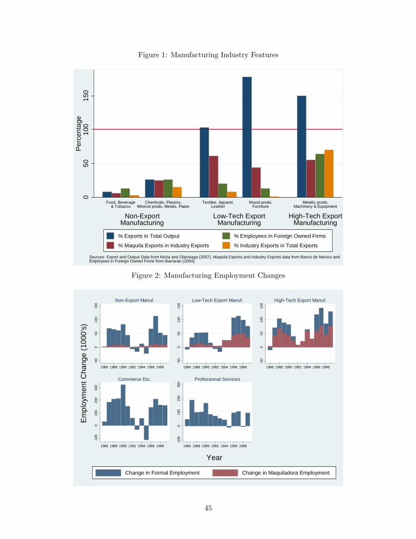
Figure 1: Manufacturing Industry Features

050

100

150

Per

cent

age

Non-ExportManufacturing

Low-Tech ExportManufacturing

High-Tech ExportManufacturing

Food, Beverage& Tobacco

Chemicals, Plastics,Mineral prods, Metals, Paper

Textiles, Apparel,Leather

Wood prods,Furniture

Metalic prods,Machinery & Equipment

Sources: Export and Output Data from Nicita and Olarreaga (2007), Maquila Exports and Industry Exports data from Banco de Mexico andEmployees in Foreign Owned Firms from Ibarraran (2004).

% Exports in Total Output % Employees in Foreign Owned Firms

% Maquila Exports in Industry Exports % Industry Exports in Total Exports

Figure 2: Manufacturing Employment Changes

-50

050

100

150

1986 1988 1990 1992 1994 1996 1998

Non-Export Manuf.

-50

050

100

150

1986 1988 1990 1992 1994 1996 1998

Low-Tech Export Manuf.

-50

050

100

150

1986 1988 1990 1992 1994 1996 1998

High-Tech Export Manuf.

-100

010

020

030

0

1986 1988 1990 1992 1994 1996 1998

Commerce Etc.

-100

010

020

030

0

1986 1988 1990 1992 1994 1996 1998

Professional Services

Em

ploy

men

t Cha

nge

(100

0's)

Year

Change in Formal Employment Change in Maquiladora Employment

45

Figure 3: Histogram of Education by Industry (2000, Insured by IMSS)

0.1

.2.3

.40

.1.2

.3.4

6 9 12 16/17 6 9 12 16/17 6 9 12 16/17

6 9 12 16/17 6 9 12 16/17 6 9 12 16/17

Non-Export Manuf. Low-Tech Export Manuf. High-Tech Export Manuf.

Commerce Etc. Professional Services Informal

Den

sity

Years of schooling

Histogram of Education by Industry (1990 and change 1990-2000, All Workers)

0.1

.2.3

6 9 12 16/17 6 9 12 16/17 6 9 12 16/17 6 9 12 16/17 6 9 12 16/17

Non-Export Manuf. Low-Tech Export Manuf. High-Tech Export Manuf. Commerce Etc. Professional Services

Pro

port

ion

of W

orke

rs (

1990

)-.

10

.1

6 9 12 16/17 6 9 12 16/17 6 9 12 16/17 6 9 12 16/17 6 9 12 16/17Cha

nge

in P

ropo

rtio

n of

Wor

kers

(19

90-2

000)

46

Figure 4: Histogram of Employee Age by Industry (2000, Insured by IMSS)

Total=580,872 Total=514,102 Total=564,639

Total=1,898,357 Total=852,217 Total=7,317,825

0.0

25.0

50

.025

.05

16 30 40 50 16 30 40 50 16 30 40 50

16 30 40 50 16 30 40 50 16 30 40 50

Non-Export Manuf. Low-Tech Export Manuf. High-Tech Export Manuf.

Commerce Etc. Professional Services Informal

Den

sity

Age

Histogram of Employee Age by Industry (1990 and change 1990-2000, All Workers)

0.0

2.0

4.0

6

16 30 40 50 16 30 40 50 16 30 40 50 16 30 40 50 16 30 40 50

Non-Export Manuf. Low-Tech Export Manuf. High-Tech Export Manuf. Commerce Etc. Professional Services

Pro

port

ion

of W

orke

rs (

1990

)-.

010

.01

16 30 40 50 16 30 40 50 16 30 40 50 16 30 40 50 16 30 40 50Cha

nge

in P

ropo

rtio

n of

Wor

kers

(19

90-2

000)

47

Figu

re5:

Visu

alIdentifi

catio

nfor20

Mun

icipalities

with

Biggest

High-Te

chEx

port

Man

ufacturin

gInflo

ws

-202 -202 -202 -202 1986

1990

1994

1998

1986

1990

1994

1998

1986

1990

1994

1998

1986

1990

1994

1998

1986

1990

1994

1998

Acu

naB

uena

vent

ura

Cam

argo

Chi

huah

uaC

once

pci

on d

el O

ro

Gom

ez F

aria

sIg

naci

o Z

arag

oza

Juár

ezM

agda

lena

Mat

amor

os

Meo

qui

Mex

ical

iN

aco

Nog

ales

Nue

vo C

asas

Gra

ndes

Nue

vo L

ared

oP

iedr

as N

egra

sR

eyno

sa-R

ío B

ravo

Tec

ate

Tiju

ana

Coh

ort A

vera

ge E

duca

tion

Net

New

Hig

h-T

ech

Exp

ort J

obs

Net New Jobs Per Worker (Normalized Residuals)

Cohort Average Education (Normalized Residuals)

Yea

r C

ohor

t Age

d 15

/16

48

Figure 6: Effect of Positive Net New Jobs per Worker Including Multiple Exposure Ages (IV)

-50

5Total Years of Schooling

-.5

0.5

1

13/14 14/15 15/16 16/17 17/18Age of Exposure

Grade 9 Dropout Rate (Inverted)

Edu

catio

nal I

mpa

ct o

f Pos

itive

Net

New

Job

s P

er W

orke

r

Non-Export Manuf. Low-Tech Export High-Tech Export Commerce etc. Professional Services

Effect of Positive Net New Jobs per Worker, Separate Regressions at Multiple Exposure Ages

-10

-50

510

1520

Edu

catio

nal I

mpa

ct o

f Pos

itive

Net

New

Job

s P

er W

orke

r

7/8 11/12 15/16 19/20 23/24Age of Exposure

Non-Export Manuf. Low-Tech Export High-Tech Export

Commerce etc. Professional Services

95 percent confidence intervals shown without markers

49

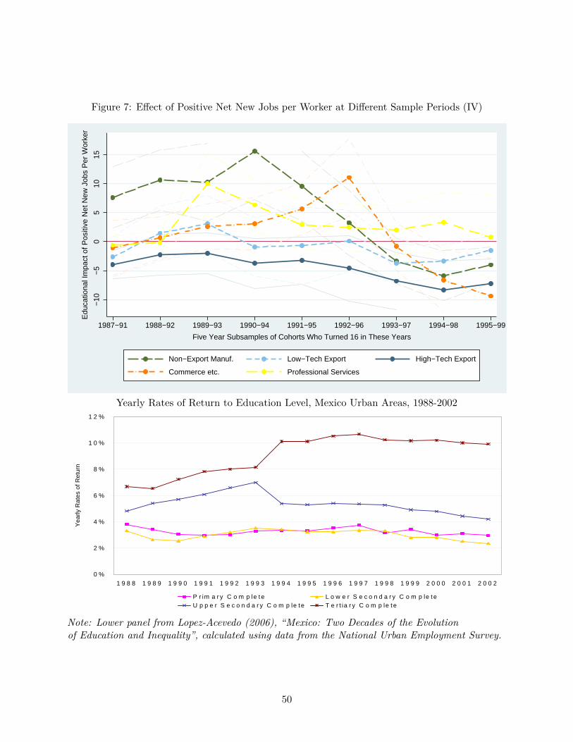
Figure 7: Effect of Positive Net New Jobs per Worker at Different Sample Periods (IV)−

10−

50

510

15

Edu

catio

nal I

mpa

ct o

f Pos

itive

Net

New

Job

s P

er W

orke

r

1987−91 1988−92 1989−93 1990−94 1991−95 1992−96 1993−97 1994−98 1995−99

Five Year Subsamples of Cohorts Who Turned 16 in These Years

Non−Export Manuf. Low−Tech Export High−Tech Export

Commerce etc. Professional Services

®

Yearly Rates of Return to Education Level, Mexico Urban Areas, 1988-2002

27

 Figure 4.1 Yearly Rates of Return to Education Level, Mexico Urban Areas, 1988-2002

0 %

2 %

4 %

6 %

8 %

1 0 %

1 2 %

1 9 8 8 1 9 8 9 1 9 9 0 1 9 9 1 1 9 9 2 1 9 9 3 1 9 9 4 1 9 9 5 1 9 9 6 1 9 9 7 1 9 9 8 1 9 9 9 2 0 0 0 2 0 0 1 2 0 0 2

Yea

rly R

ates

of R

etur

n

P r im a r y C o m p le t e L o w e r S e c o n d a r y C o m p le t eU p p e r S e c o n d a r y C o m p le te T e r t ia r y C o m p le t e  

Note: The yearly rate of return represents the additional contribution to wages from an additional year of a certain level of education. All the coefficients are statistically significant at the 5 per cent level and conditioned on age, squared age, gender, region (North, Center, South, and Mexico City).

Source: Calculations using third quarter of the National Urban Employment Survey (ENEU) from 1988 to 2001 and third quarter and urban section of ENET 2002.

Note: Lower panel from Lopez-Acevedo (2006), “Mexico: Two Decades of the Evolutionof Education and Inequality”, calculated using data from the National Urban Employment Survey.

50

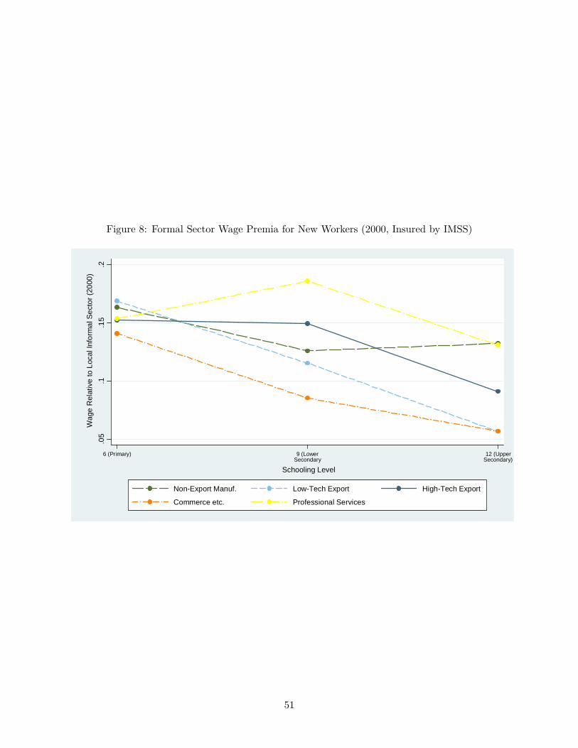
Figure 8: Formal Sector Wage Premia for New Workers (2000, Insured by IMSS)

.05

.1.1

5.2

Wag

e R

elat

ive

to L

ocal

Info

rmal

Sec

tor

(200

0)

6 (Primary) 9 (LowerSecondary

12 (UpperSecondary)

Schooling Level

Non-Export Manuf. Low-Tech Export High-Tech Export

Commerce etc. Professional Services

51

Figure 9: Returns to Schooling for New Workers (2000, Insured by IMSS)

0.5

1

Wag

e R

elat

ive

to L

ower

Sec

onda

ry (

2000

)

6 (Primary) 9 (LowerSecondary

12 (UpperSecondary)

College(16-17)

Schooling Level

Non-Export Manuf. Low-Tech Export High-Tech Export

Commerce etc. Professional Services

Tenure-Wage Profile for Different Levels of Schooling (2000, Insured by IMSS)

0.5

11.

5

16 19 23 30 35 40

Non-Export Manuf.

16 19 23 30 35 40

Low-Tech Export Manuf.

16 19 23 30 35 40

High-Tech Export Manuf.

0.5

11.

5

16 19 23 30 35 40

Commerce Etc.

16 19 23 30 35 40

Professional Services

6 Years of School

9 Years of School

12 Years of School

16/17 Years of School

Mal

e W

age

Rel

ativ

e to

Info

rmal

Sec

tor

with

9 Y

ears

of S

choo

l and

No

Exp

erie

nce

Age

52

Table 1: Sample Means

Census Schooling Sample (2000, Age 16-28, Non Migrants, Excludes Mexico City)mean standard deviation observations

Age 21.54 0.0038 1,706,582Years of School 8.51 0.0038 1,636,520Attending School (1=yes, 0=no) 0.21 0.0004 1,696,172Employed (1=yes, 0=no) 0.52 0.0005 1,706,582Insured by IMSS (1=yes, 0=no) 0.42 0.0011 1,706,582Monthly Log Earned Income (Pesos) 7.47 0.0011 667,103Sex (1=male, 0=female) 0.48 0.0005 1,706,582Municipality Size 8540.26 816.7 1808

IMSS Annual Firm Sample (1985-2000)mean standard deviation observations

Firm Size (Employees) 12.08 0.044 11,365,321Firm Size (Firms Changing Employment) 16.03 0.065 7,675,094Firm Size (Firms Hiring/Firing≥ 50 in single year) 416.41 4.140 109,263Proportion Male Workers 0.68 11,365,321Unique Firms 2,194,681Employees (1985) 4,472,491Firms (1985) 372,520Employees (2000) 12,509,298Firms (2000) 912,284

53

Table2:

Tran

sitionMatrix

forNet

New

Jobs

PerWorker

NextPe

riods

Value

NextPe

riods

Value

NextPe

riods

Value

Initial

Value

Negative

Zero

Posit

ive

Negative

Zero

Posit

ive

Negative

Zero

Posit

ive

Non

Expo

rtMan

uf.

Low-TechEx

port

Man

uf.

High-Te

chEx

port

Man

uf.

Negative

53.03

3.10

43.87

53.76

2.87

43.38

51.08

4.13

44.79

Zero

4.94

91.84

3.23

3.94

94.7

1.36

3.79

94.4

1.81

Posit

ive

18.51

6.12

75.37

18.04

8.44

73.52

18.83

10.29

70.88

Com

merce

etc.

Professio

nalS

ervices

Negative

51.65

1.79

46.55

48.85

2.67

48.47

Zero

5.22

90.72

4.06

2.51

93.98

3.51

Posit

ive

15.23

3.30

81.47

11.09

6.78

82.13

54

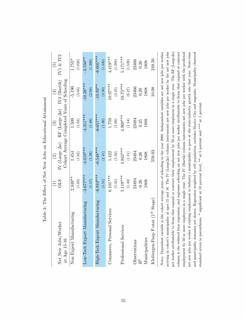
Table3:

The

Effectof

Net

New

Jobs

onEd

ucationa

lAttainm

ent

(1)

(2)

(3)

(4)

(5)

Net

New

Jobs/W

orker

OLS

IV(L

arge

∆s)

RF(L

arge

∆s)

IV2(B

artik

)IV

1&

IV2

atAge

15-16

Coh

ortAv

erag

eCom

pleted

Yearsof

Scho

oling

Non

Expo

rtMan

ufacturin

g2.34

9**

1.45

41.50

9-5.190

1.75

5*(1.03)

(1.02)

(1.03)

(4.04)

(1.026)

Low-TechEx

port

Man

ufacturin

g-3.677

***

-4.019

***

-4.311

***

-10.38

***

-3.550

**(1.17)

(1.39)

(1.48)

(2.94)

(1.386)

High-Te

chEx

port

Man

ufacturin

g-6.910

***

-6.548

***

-6.657

***

-10.93

**-6.605

***

(1.51)

(1.41)

(1.46)

(4.36)

(1.440)

Com

merce,P

ersona

lServices

6.10

1***

1.42

21.75

910

.97*

**4.41

9***

(1.31)

(1.32)

(1.60)

(3.45)

(1.388)

Professio

nalS

ervices

5.11

9***

4.94

2***

4.96

9***

19.75*

**5.17

1***

(1.49)

(1.51)

(1.54)

(6.27)

(1.538)

Observatio

ns23

484

2348

423

484

2346

623

466

R2

0.26

0.26

0.25

0.20

0.26

Mun

icipalities

1808

1808

1808

1808

1808

Kleibergen-Pa

apF-stat

(1st

Stag

e)55

8.03

10.08

249.50

Not

es:Dep

endent

varia

bleis

thecoho

rtaverag

eyearsof

scho

olingin

theyear

2000

.Inde

pend

entvaria

bles

arene

tne

wjobs

perwo

rker

arriv

ingin

coho

rt’s

mun

icipality

atag

es15

and16.The

IV(L

arge

∆s)

columninstruments

netne

wjobs

perwo

rker

bythene

tne

wjobs

perwo

rker

attributab

leto

firmsthat

expa

ndor

contract

theirem

ploymentby

50or

moreem

ployeesin

asin

gleyear.The

RF(L

arge

∆s)

columnis

theredu

cedform

regressio

n,an

dregressesscho

olingon

netne

wjobs

perwo

rker

attributab

leto

firmsthat

expa

ndor

contract

employmentby

50or

moreem

ployeesin

asin

gleyear.The

IV(B

artik

)columninstruments

netne

wjobs

perworkerwith

thepred

icted

netne

wjobs

perwo

rker

ifexist

ingem

ploymentin

indu

stryimun

icipality

mgrew

atthestate-indu

stry

grow

thrate

that

year.State-tim

ean

dmun

icipality

dummiesno

tshow

n.Regressionwe

ighted

bycellpo

pulatio

n,exclud

esMexicoCity

andmigrants.

Mun

icipality

clustered

stan

dard

errors

inpa

renthe

ses.

*sign

ificant

at10

percentlevel,**

at5pe

rcentan

d***at

1pe

rcent.

55

Table 4: The Assymetric Effect of Net New Jobs on Educational Attainment

LHS: Cohort Average (1) (2) (3)Years of School OLS IV (Large ∆s) RF (Large ∆s)

Positive Net New Jobs Per Worker at Ages 15-16Non Export 5.119*** 3.870*** 4.175***Manufacturing (1.53) (1.39) (1.41)

Low-Tech Export -3.601** -3.862** -4.095**Manufacturing (1.46) (1.70) (1.82)

High-Tech Export -8.056*** -7.674*** -7.741***Manufacturing (1.86) (1.75) (1.80)

Commerce, 8.405*** 2.708 3.775Personal Services (1.82) (1.97) (2.50)

Professional 9.150*** 8.123*** 8.378***Services (3.17) (2.90) (3.04)

Negative Net New Jobs Per Worker at Ages 15-16Non Export -2.394 -2.510 -2.406Manufacturing (1.58) (1.70) (1.67)

Low-Tech Export -4.398* -4.917 -5.195*Manufacturing (2.51) (3.01) (2.89)

High-Tech Export -5.808* -4.169 -4.259Manufacturing (3.13) (3.15) (3.21)

Commerce, -4.004** -2.521 -1.832Personal Services (1.72) (2.56) (2.15)

Professional -13.11*** -9.315*** -8.052***Services (2.79) (2.47) (2.13)

Observations 23484 23484 23484R2 0.27 0.27 0.26Municipalities 1808 1808 1808Kleibergen-Paap rk Wald F-stat (1st Stage) 86.50

Notes: Dependent variable is the cohort average years of schooling in the year 2000. Independent variables arenet new jobs per worker arriving in cohort’s municipality at ages 15 and 16 interacted with a dummy variable thattakes the value 1 if net new jobs per worker is positive, and another dummy variable that takes the value 1 if netnew jobs per worker is negative. The IV (Large∆s) column instruments (interacted) net new jobs per worker bythe (interacted) net new jobs per worker attributable to firms that expand or contract their employment by 50or more employees in a single year. The RF (Large∆s) column is the reduced form regression, and regressesschooling on (interacted) net new jobs per worker attributable to firms that expand or contract employment by 50or more employees in a single year. State-time and municipality dummies not shown. Regression weighted bycell population, excludes Mexico City and migrants. Municipality clustered standard errors in parentheses. *significant at 10 percent level, ** at 5 percent and *** at 1 percent.

56

Table 5: The Effect of Net New Jobs at Multiple Ages on Educational Attainment

LHS: Cohort Average (1)Years of School IV (Large ∆s)Positive Net New Jobs Per Worker at: Ages 13/14 Ages 14/15 Ages 15/16 Ages 16/17 Ages 17/18Non Export 2.910 5.586** -0.923 3.646 0.968Manufacturing (2.364) (2.579) (2.968) (2.294) (1.821)

Low-Tech Export -4.000** 1.880 -5.022** 1.058 -2.550Manufacturing (1.845) (1.996) (2.161) (1.692) (1.658)

High-Tech Export -3.277 1.762 -5.313*** 0.854 -3.468*Manufacturing (2.018) (1.697) (1.888) (1.747) (2.030)

Commerce, 1.460 7.909*** -0.808 0.995 -2.294Personal Services (2.487) (3.062) (3.012) (2.404) (2.647)

Professional 4.267*** 1.603 4.711** 3.476* -1.996Services (1.231) (1.548) (1.938) (1.992) (3.694)

Negative Net New Jobs Per Worker at: Ages 13/14 Ages 14/15 Ages 15/16 Ages 16/17 Ages 17/18Non Export -3.444 1.498 -0.935 -2.576 6.194Manufacturing (2.731) (3.611) (3.823) (2.847) (4.045)

Low-Tech Export -6.898 3.621 -3.714 3.031 -8.901***Manufacturing (4.219) (3.692) (4.391) (3.940) (3.416)

High-Tech Export 0.886 5.892** -3.029 -0.000996 -2.024Manufacturing (2.641) (2.499) (2.628) (2.032) (2.146)

Commerce, -4.997 2.811 -2.335 7.044* -3.729Personal Services (3.237) (3.831) (3.689) (3.870) (2.727)

Professional 8.326 -0.0191 -0.487 -6.091** 2.342Services (6.351) (2.144) (3.889) (2.380) (3.421)

Observations 16257R2 0.2Municipalities 1808Notes: Dependent variable is the cohort average years of schooling in the year 2000. Independent variables are net new jobsper worker arriving in cohort’s municipality at ages 13/14 through 17/18 interacted with a dummy variable that takesthe value 1 if net new jobs per worker is positive, and another dummy variable that takes the value 1 if net new jobs perworker is negative. The IV (Large∆s) column instruments (interacted) net new jobs per worker by the (interacted) netnew jobs per worker attributable to firms that expand or contract their employment by 50 or more employees in a singleyear. State-time and municipality dummies not shown. Regression weighted by cell population, excludes Mexico City andmigrants. Municipality clustered standard errors in parentheses. * significant at 10 percent level, ** at 5 percent and *** at1 percent.

57

Table6:

Dire

ctan

dIndirect

Cha

nnels

(1)

(2)

(3)

(4)

(5)

(6)

LHS:

Grade

7Grade

9Grade

12Pr

oportio

nTe

ch.

Coh

ortAv

g.Coh

ortAv

g.(A

llLa

rge

∆sIV

)Dropo

utRateDropo

utRateDropo

utRate

Ed.Stud

ents

Yearsof

Scho

olYe

arsof

Scho

olPo

sitiveNet

New

Jobs

PerWorker:

atAges12

-13at

Ages15

-16at

Ages18

-19

atAges15

-16

atAges15

-16

atAges15

-16

Non

Expo

rt0.04

28-0.196

-0.424

0.00

864.48

4***

4.37

4**

Man

ufacturin

g(0.166)

(0.199)

(0.332)

(0.17)

(1.387)

(2.07)

Low-TechEx

port

0.59

6***

0.13

9-0.253

-0.247

**-3.750

**-2.701

Man

ufacturin

g(0.186)

(0.185)

(0.358)

(0.12)

(1.723)

(4.30)

High-Te

chEx

port

0.52

6***

0.44

3**

-0.130

-0.331

***

-7.283

***

-8.469

**Man

ufacturin

g(0.144)

(0.179)

(0.224)

(0.12)

(1.798)

(4.28)

Com

merce,

-0.407

***

0.08

170.25

8-0.013

5-0.327

Person

alSe

rvices

(0.157)

(0.177)

(0.364)

(0.12)

(2.55)

Professio

nal

-0.695

***

-0.227

*0.10

80.33

4*-2.442

Services

(0.229)

(0.131)

(0.147)

(0.17)

(5.49)

Posit

iveNet

New

FemaleJo

bsPe

rWorker:

atAges15

-16

Non

Expo

rt-0.921

Man

ufacturin

g(3.54)

Low-TechEx

port

-1.227

Man

ufacturin

g(3.94)

High-Te

chEx

port

0.97

0Man

ufacturin

g(3.55)

Com

merce,

6.30

2Pe

rson

alSe

rvices

(5.22)

Professio

nal

11.62*

*Se

rvices

(5.55)

Observatio

ns23

466

2240

917

565

2262

223

484

2348

4R

20.52

0.41

0.25

0.64

0.25

0.27

Mun

icipalities

1808

1806

1696

1807

1808

1808

Not

es:Dep

ende

ntvaria

bles

arethecoho

rtaverageyearsof

scho

olingin

theyear

2000,t

heprop

ortio

nof

second

aryan

dhigh

scho

olstud

ents

who

take

thetechnical

educationrather

than

gene

rale

ducatio

ntrackan

dtheprop

ortio

nof

acoho

rtwho

reache

sgrad

es6,

9an

d12

butgo

esno

furthe

r.Inde

pend

entvaria

bles

arene

tne

wjobs

perwo

rker

arriv

ingin

coho

rt’s

mun

icipality

atthegivenexpo

sure

ages

interacted

with

adu

mmyvaria

blethat

takesthevalue1ifne

tne

wjobs

perwo

rker

ispo

sitive,

and

anothe

rdu

mmyvaria

blethat

takesthevalue1ifne

tne

wjobs

perworkeris

negativ

e.Negativene

tne

wjobpe

rworkerresults

notshow

n.Allcolumns

instrument

(interacted

)ne

tne

wjobs

perwo

rker

bythe(in

teracted

)ne

tne

wjobs

perwo

rker

attributab

leto

firmsthat

expa

ndor

contract

theirem

ploymentby

50or

moreem

ployees

inasin

gleyear.State-tim

ean

dmun

icipality

dummiesno

tshow

n.Regressionweigh

tedby

cellpo

pulatio

n,exclud

esMexicoCity

andmigrants.

Mun

icipality

clustered

stan

dard

errors

inpa

renthe

ses.

*sign

ificant

at10

percentlevel,**

at5pe

rcentan

d***at

1pe

rcent.

58

Table7:

Rob

ustnessChe

cks1:

Other

Specificatio

ns

LHS:

Coh

ortAv

erage

(1)

(2)

(3)

(4)

(5)

(6)

(7)

(8)

(9)

Yearsof

Scho

olBasic

IVMun

i.Tr

end

Cap

at12

Not

atScho

olMen

Only

Wom

enOnly|∆l m

ci|≥

100

Form

alMun

i.Rural

Trend

Posit

iveNet

New

Jobs

PerWorkerat

Ages15-16

Non

Expo

rt3.870***

1.409

1.913**

1.778

2.539**

5.747**

4.723***

3.592***

2.806**

Man

ufacturin

g(1.388)

(1.254)

(0.950)

(1.201)

(1.10)

(2.54)

(1.49)

(1.39)

(1.319)

Low-TechEx

port

-3.862**

-1.039

-3.408***

-3.934**

-3.975**

-3.440**

-3.866**

-1.685

-2.451*

Man

ufacturin

g(1.699)

(0.960)

(1.204)

(1.596)

(1.78)

(1.74)

(1.97)

(1.88)

(1.410)

High-Te

chEx

port

-7.674***

-3.417***

-4.904***

-5.426***

-5.880***

-6.211***

-7.745***

-7.572***

-5.708***

Man

ufacturin

g(1.752)

(1.149)

(1.162)

(1.320)

(1.92)

(2.11)

(1.78)

(1.65)

(1.343)

Com

merce,

2.708

-2.388**

1.568

2.257

0.582

6.533

2.515

3.353*

2.096

Person

alServices

(1.975)

(1.178)

(1.425)

(1.606)

(1.32)

(4.08)

(2.12)

(1.96)

(1.499)

Professio

nal

8.123***

-3.874***

4.453**

4.694**

6.376***

8.479**

7.915***

7.573***

4.012***

Services

(2.897)

(1.105)

(1.779)

(1.907)

(2.14)

(3.42)

(2.86)

(2.64)

(1.405)

NegativeNet

New

Jobs

PerWorkerat

Ages15-16

Non

Expo

rt-2.510

-1.525

-1.655

-2.125*

-0.773

-10.04***

-3.246*

-1.849

-1.572

Man

ufacturin

g(1.696)

(1.469)

(1.162)

(1.191)

(1.34)

(3.72)

(1.79)

(1.73)

(1.707)

Low-TechEx

port

-4.917

-0.0679

-1.413

-3.651

-3.195

0.886

-6.187*

-5.869**

-2.601

Man

ufacturin

g(3.010)

(2.647)

(2.347)

(2.802)

(3.34)

(3.89)

(3.43)

(2.93)

(2.680)

High-Te

chEx

port

-4.169

-2.475

-3.348

-1.494

-5.959***

1.016

-3.945

-4.063

-3.069

Man

ufacturin

g(3.146)

(2.298)

(2.376)

(2.319)

(1.87)

(2.01)

(3.28)

(3.16)

(3.085)

Com

merce,

-2.521

-0.501

-1.469

-0.533

-0.280

-11.18

-2.178

-3.225

-3.075

Person

alServices

(2.555)

(1.864)

(1.712)

(2.105)

(1.47)

(17.3)

(2.74)

(2.53)

(2.222)

Professio

nal

-9.315***

-3.624**

-6.195***

-5.381***

-6.592**

-7.571***

-7.494***

-9.530***

-9.659***

Services

(2.468)

(1.694)

(1.727)

(1.857)

(2.79)

(2.40)

(2.28)

(2.41)

(1.991)

Observatio

ns23484

23484

23484

23477

23328

23375

23484

13350

23484

R2

0.27

0.56

0.29

0.42

0.20

0.21

0.27

0.31

0.41

Mun

icipalities

1808

1808

1808

1808

1808

1808

1808

1027

1808

Not

es:Dep

ende

ntvaria

bleisthecoho

rtaverageyearsof

scho

olingin

theyear

2000.Inde

pend

entvaria

bles

arene

tne

wjobs

perwo

rker

arriv

ingin

coho

rt’smun

icipality

atag

es15

and16

.The

sevaria

bles

areinstrumentedby

thene

tne

wjobs

perwo

rker

attributab

leto

firmsthat

expa

ndor

contract

theirem

ploymentby

morethan

50em

ployeesin

asin

gleyear.Sp

ecificatio

nsde

scrib

edin

section5.

State-tim

ean

dmun

icipality

dummiesno

tshow

n.Regressionweigh

tedby

cellpo

pulatio

n,exclud

esMexicoCity

andmigrants.

Mun

icipality

clusteredstan

dard

errors

inpa

renthe

ses.

*sign

ificant

at10

percentlevel,**

5pe

rcentan

d***1pe

rcent.

59

Table8:

Rob

ustnessChe

cks2:

Regiona

lEffe

cts

LHS:

Coh

ortAv

erage

(10)

(11)

(12)

(13)

(14)

(15)

(16)

(17)

(18)

(19)

(20)

Yearsof

Scho

olNoBig

City

Mex.City

OnlyZM

NoZM

North

Central

South

Low

Skill

HighSk

illRicher

Poorer

Posit

iveNet

New

Jobs

PerWorkerat

Ages15-16

Non

Expo

rt3.334**

6.625***

2.022

0.502

7.286***

1.118

5.068**

0.477

4.811***

3.398*

3.321**

Man

ufacturin

g(1.321)

(1.818)

(2.939)

(1.585)

(2.395)

(2.612)

(2.088)

(1.457)

(1.793)

(1.825)

(1.656)

Low-TechEx

port

-5.033***

-0.425

3.299

-4.751***

-3.368

-3.973*

-9.004

-6.084**

-0.749

-3.770**

-10.46***

Man

ufacturin

g(1.717)

(2.448)

(4.429)

(1.795)

(2.434)

(2.395)

(8.483)

(2.944)

(1.703)

(1.687)

(3.035)

High-Te

chEx

port

-4.961***

-6.524**

-3.785*

-3.867***

-5.477***

-27.06***

9.632

1.086

-6.795***

-6.037***

-8.220***

Man

ufacturin

g(1.574)

(2.660)

(2.226)

(1.357)

(1.604)

(7.978)

(24.78)

(2.449)

(1.490)

(1.597)

(2.647)

Com

merce,

3.449*

4.125*

-10.79***

4.381**

5.788***

-5.220

7.853**

7.014

2.236

-1.317

4.823**

Person

alServices

(1.823)

(2.398)

(3.318)

(1.724)

(2.213)

(3.741)

(3.605)

(4.284)

(1.813)

(2.017)

(2.406)

Professio

nal

6.274**

8.350***

2.317*

9.552***

15.97***

8.262***

-1.953

-3.949

7.154***

6.372***

6.507

Services

(2.502)

(3.150)

(1.244)

(2.955)

(3.719)

(2.824)

(16.20)

(3.714)

(2.380)

(2.391)

(4.180)

NegativeNet

New

Jobs

PerWorkerat

Ages15-16

Non

Expo

rt-1.715

-2.785

1.480

-0.221

-4.725

-6.170**

2.496

-2.179

-1.603

-2.650

-2.697

Man

ufacturin

g(1.625)

(1.839)

(3.106)

(1.801)

(3.749)

(2.705)

(2.007)

(2.188)

(1.872)

(1.950)

(3.742)

Low-TechEx

port

-3.735

-5.939

16.11

2.664

-7.249

-1.940

-22.81

23.25***

-7.976***

-4.855

2.048

Man

ufacturin

g(3.001)

(3.828)

(15.45)

(2.959)

(5.822)

(3.179)

(15.05)

(5.679)

(2.980)

(4.504)

(4.213)

High-Te

chEx

port

-5.504*

-4.009

-6.738

-2.381

-1.549

4.253

-23.65

66.68

-4.033

-4.175

4.297

Man

ufacturin

g(3.213)

(3.545)

(7.616)

(3.208)

(4.570)

(5.574)

(14.98)

(45.47)

(3.138)

(3.543)

(4.669)

Com

merce,

-3.399

-2.933

-3.657

-1.196

-7.829**

6.296

0.0768

1.021

-2.656

-0.756

2.793

Person

alServices

(2.371)

(2.684)

(13.33)

(1.925)

(3.414)

(5.349)

(6.185)

(2.131)

(2.934)

(4.231)

(2.532)

Professio

nal

-6.255***

-7.942***

-9.832**

-6.659***

-13.01***

-11.81**

2.132

18.71***

-9.806***

-8.620***

-9.325

Services

(2.135)

(2.379)

(4.101)

(2.433)

(2.799)

(4.828)

(25.70)

(7.041)

(2.405)

(2.456)

(8.155)

Observatio

ns23458

23497

702

22782

4302

9789

9393

11739

11745

11748

11736

R2

0.23

0.37

0.80

0.16

0.49

0.19

0.18

0.32

0.41

0.36

0.32

Mun

icipalities

1806

1809

541754

331

753

724

904

904

904

904

Not

es:Dep

ende

ntvaria

bleis

thecoho

rtaverageyearsof

scho

olingin

theyear

2000.Inde

pend

entvaria

bles

arene

tne

wjobs

perwo

rker

arriv

ingin

coho

rt’s

mun

icipality

atag

es15

and16

.The

sevaria

bles

areinstrumentedby

thene

tne

wjobs

perworkerattributab

leto

firmsthat

expa

ndor

contract

theirem

ploymentby

50or

more

employeesin

asin

gleyear.Sp

ecificatio

nsde

scrib

edin

section5.

State-tim

ean

dmun

icipality

dummiesno

tshow

n.Colum

ns14

,15an

d16

includ

eregion

-tim

edu

mmies

forsix

region

sof

Mexicoinsteadof

state-tim

edu

mmies.

Cellp

opulationweigh

ts,e

xclude

sMexicoCity

(excep

tforcolumn14

)an

dmigrants.

Mun

icipality

clustered

stan

dard

errors

inpa

renthe

ses.

*sign

ificant

at10

percentlevel,**

5pe

rcentan

d***1pe

rcent.

60

Table9:

The

Effectof

Net

New

Jobs

onEd

ucationa

lAttainm

entby

Indu

stry

Cha

racterist

ics

(1)

(2)

(3)

(4)

(5)

(6)

IVSp

ecificatio

nLH

S:Coh

ortAv

erag

eYe

arsof

Scho

olPo

sitiveNet

New

Jobs

PerWorker

3.28

5***

4.39

8***

4.43

8***

182.7*

**27

.45

54.52

(AllIndu

strie

s,AllFirm

s)(1.011)

(1.202)

(1.211)

(43.88)

(56.47)

(61.23)

I+

∑ j∈m(N

ewJo

bsPe

rWorker j

-7.017

***

-0.612

0.86

15.31

9**

5.38

3**

×Maq

uilado

raIndicator j)

(1.696)

(1.841)

(2.013)

(2.671)

(2.727)

I+

∑ i′(N

ewJo

bsPe

rWorker i′

-0.038

0***

-0.036

5***

0.00

0716

0.06

05**

0.05

86*

×Ex

port

i′mex

Outpu

t i′mex

)(0.00857)

(0.0101)

(0.0125)

(0.0246)

(0.0336)

I+

∑ i′(N

ewJo

bsPe

rWorker i′

-241

.3**

*85

.37

87.09

×pmex

(New

Jobsi′t+

1>0|New

Jobsi′t>

0))

(62.90)

(108.9)

(112.7)

I+

∑ i′(N

ewJo

bsPe

rWorker i′

-69.58

***

-48.11

***

-52.42

***

×Em

ployee

Sharewith

S<

12i′mex

)(14.86)

(14.30)

(17.66)

I+

∑ i′(N

ewJo

bsPe

rWorker i′

-41.87

-113

.2*

×Em

ployee

Share≤

3yrsou

tscho

oli′mex

)(124.4)

(68.46)

I+

∑ i′(N

ewJo

bsPe

rWorker i′

-0.618

***

-0.858

***

-12.03

***

×Wag

ePr

emium

(S=9)i′mex

Wag

ePr

emium

(S=12

) i′mex

)(0.181

)(0.186)

(2.778)

I+

∑ j∈m(N

ewJo

bsPe

rWorker j

-0.000

185*

-5.87e-05

×Firm

Employees j)

(0.000108)

(0.000126)

I+

∑ i′(N

ewJo

bsPe

rWorker i′

-436

.1**

*-305

.6**

*×Indu

stry

MeanGrowth

Rate i′ m

ex)

(156.2)

(115.6)

Cen

susUsedFo

r3-digitIndu

stry

Averag

es23

484

2348

423

484

2348

423

484

2348

4Observatio

ns0.25

0.26

0.26

0.25

0.27

0.27

R2

1808

1808

1808

1808

1808

1808

Mun

icipalities

1808

1808

1808

1808

1808

1808

Not

es:Dep

ende

ntvaria

bleis

coho

rtaverageyearsof

scho

olingin

year

2000.Inde

pend

entvaria

bles

arene

tne

wjobs

perwo

rker

arriv

ingin

coho

rt’s

mun

icipality

atages

15an

d16

interacted

with

posit

ivean

dne

gativ

eindicatorvaria

bles.Negativene

wne

wjobs

coeffi

cients

notshow

n.Interacted

netne

wjobs

perworkerterm

sinstrumentedwith

interactions

ofne

tne

wjobs

perworkerattributab

leto

firmsthat

expa

ndor

contract

their

employmentby

50or

moreem

ployeesin

asin

gleyear.Add

ition

alne

wjobs

term

sareinteractions

betw

eenfirm/3

-digit

indu

stry

jobarriv

alsan

dfirm/3-digitindu

stry

characteris

tics(firm

Maq

uilado

rastatus,p

ropo

rtionof

natio

nalind

ustryou

tput

expo

rted

1986-1999,

natio

nalind

ustrytran

sition

prob

abilitie

sof

twoconsecutiveyearsof

posit

ivene

wjobarriv

als19

86-199

9,prop

ortio

nof

natio

nalind

ustryem

ployeeswith

less

than

12yearsof

scho

olingin

either

theyear

2000

or1990,p

ropo

rtionof

natio

nalind

ustryem

ployeesou

tof

scho

olfor3yearsor

less

in1990

or2000,n

ationa

lind

ustry

“wag

eprem

ia”forem

ployeeswith

second

aryscho

oldivide

dby

prem

iaforthosewith

high

scho

olin

1990

or20

00,n

umbe

rof

firm

employeesan

dna

tiona

lind

ustrymeanjobgrow

th).

State-tim

ean

dmun

icipality

dummiesno

tshow

n.Regressionwe

ighted

bycellpo

pulatio

n,exclud

esMexicoCity

andmigrants.

Mun

icipality

clusteredstan

dard

errors

inpa

renthe

ses.

*sign

ificant

at10

percentlevel,**

at5pe

rcentan

d***at

1pe

rcent.

61

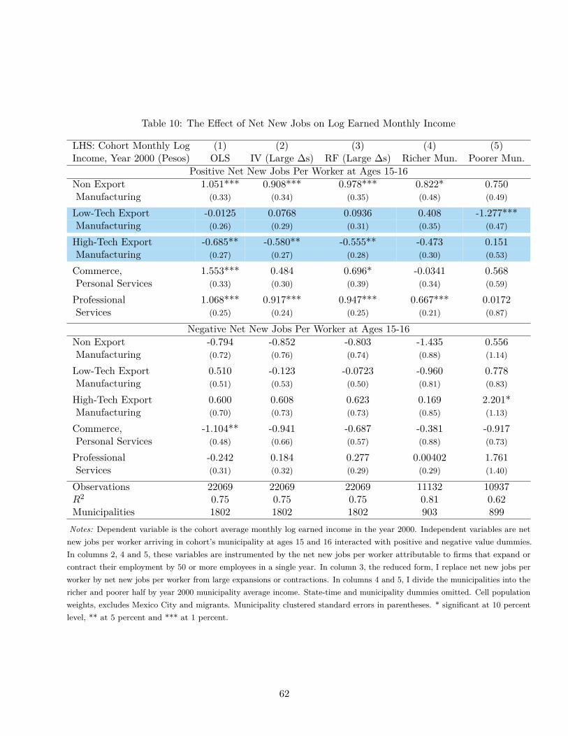
Table 10: The Effect of Net New Jobs on Log Earned Monthly Income

LHS: Cohort Monthly Log (1) (2) (3) (4) (5)Income, Year 2000 (Pesos) OLS IV (Large ∆s) RF (Large ∆s) Richer Mun. Poorer Mun.

Positive Net New Jobs Per Worker at Ages 15-16Non Export 1.051*** 0.908*** 0.978*** 0.822* 0.750Manufacturing (0.33) (0.34) (0.35) (0.48) (0.49)

Low-Tech Export -0.0125 0.0768 0.0936 0.408 -1.277***Manufacturing (0.26) (0.29) (0.31) (0.35) (0.47)

High-Tech Export -0.685** -0.580** -0.555** -0.473 0.151Manufacturing (0.27) (0.27) (0.28) (0.30) (0.53)

Commerce, 1.553*** 0.484 0.696* -0.0341 0.568Personal Services (0.33) (0.30) (0.39) (0.34) (0.59)

Professional 1.068*** 0.917*** 0.947*** 0.667*** 0.0172Services (0.25) (0.24) (0.25) (0.21) (0.87)

Negative Net New Jobs Per Worker at Ages 15-16Non Export -0.794 -0.852 -0.803 -1.435 0.556Manufacturing (0.72) (0.76) (0.74) (0.88) (1.14)

Low-Tech Export 0.510 -0.123 -0.0723 -0.960 0.778Manufacturing (0.51) (0.53) (0.50) (0.81) (0.83)

High-Tech Export 0.600 0.608 0.623 0.169 2.201*Manufacturing (0.70) (0.73) (0.73) (0.85) (1.13)

Commerce, -1.104** -0.941 -0.687 -0.381 -0.917Personal Services (0.48) (0.66) (0.57) (0.88) (0.73)

Professional -0.242 0.184 0.277 0.00402 1.761Services (0.31) (0.32) (0.29) (0.29) (1.40)

Observations 22069 22069 22069 11132 10937R2 0.75 0.75 0.75 0.81 0.62Municipalities 1802 1802 1802 903 899

Notes: Dependent variable is the cohort average monthly log earned income in the year 2000. Independent variables are netnew jobs per worker arriving in cohort’s municipality at ages 15 and 16 interacted with positive and negative value dummies.In columns 2, 4 and 5, these variables are instrumented by the net new jobs per worker attributable to firms that expand orcontract their employment by 50 or more employees in a single year. In column 3, the reduced form, I replace net new jobs perworker by net new jobs per worker from large expansions or contractions. In columns 4 and 5, I divide the municipalities into thericher and poorer half by year 2000 municipality average income. State-time and municipality dummies omitted. Cell populationweights, excludes Mexico City and migrants. Municipality clustered standard errors in parentheses. * significant at 10 percentlevel, ** at 5 percent and *** at 1 percent.

62

Table 11: The Effect of Net New Jobs on Income and Participation by Gender

(1) (2) (3) (4) (5) (6)LHS: (All Large ∆s IV) Cohort Log Income, 2000 Cohort Labor Force Participation, 2000Gender: All Male Female All Male Female

Positive Net New Jobs Per Worker at Ages 15-16Non Export 0.908*** 0.351 1.896** 0.246 0.263* 0.167Manufacturing (0.337) (0.226) (0.799) (0.164) (0.157) (0.414)

Low-Tech Export 0.0768 0.349 -0.628 0.376** 0.0404 0.506**Manufacturing (0.290) (0.286) (0.476) (0.169) (0.185) (0.229)

High-Tech Export -0.580** -0.383 -0.428 -0.274** -0.229 -0.232*Manufacturing (0.272) (0.240) (0.346) (0.133) (0.143) (0.120)

Commerce, 0.484 0.124 0.922 0.0798 0.0594 0.320Personal Services (0.296) (0.229) (0.685) (0.152) (0.110) (0.345)

Professional 0.917*** 0.753*** 1.086*** 0.574*** 0.222 0.721***Services (0.242) (0.243) (0.241) (0.183) (0.147) (0.201)

Negative Net New Jobs Per Worker at Ages 15-16Non Export -0.852 -0.239 -1.361 0.0855 -0.146 1.184*Manufacturing (0.760) (0.494) (1.719) (0.306) (0.180) (0.710)

Low-Tech Export -0.123 -0.0542 -1.066 -1.086*** 0.0876 -1.877**Manufacturing (0.531) (0.399) (0.974) (0.360) (0.227) (0.813)

High-Tech Export 0.608 0.145 0.654 -0.180 -0.120 -0.256Manufacturing (0.733) (0.502) (0.498) (0.342) (0.266) (0.529)

Commerce, -0.941 -0.295 -3.847 -0.304 -0.0969 -2.205Personal Services (0.657) (0.342) (4.644) (0.282) (0.136) (1.967)

Professional 0.184 0.220 -0.0808 -1.002*** -1.013*** -0.0103Services (0.317) (0.401) (0.469) (0.219) (0.237) (0.256)

Observations 22069 21426 18383 23479 23314 23364R2 0.75 0.68 0.57 0.26 0.56 0.13Municipalities 1802 1799 1735 1808 1808 1808Notes: Dependent variable is the cohort average monthly log earned income in the year 2000 or the cohort average labor forceparticipation for workers not at school, broken down by gender. Independent variables are net new jobs per worker arriving incohort’s municipality at ages 15 and 16 interacted with positive and negative value dummies. These variables are instrumented bythe net new jobs per worker attributable to firms that expand or contract their employment by 50 or more employees in a singleyear. State-time and municipality dummies omitted. Cell population weights, excludes Mexico City and migrants. Municipalityclustered standard errors in parentheses. * significant at 10 percent level, ** at 5 percent and *** at 1 percent.

63

Table 12: The Effect of Net New Jobs on Cohort Size and Selective Migration

(1) (2)Log Cohort Size Ratio of Leavers Schooling

to Stayers (1995-1999)Positive Net New Jobs Per Worker at Ages 15-16

Non Export 0.353 -0.434Manufacturing (0.51) (0.59)

Low-Tech Export -0.512 -0.787*Manufacturing (0.40) (0.47)

High-Tech Export -0.283 -1.061***Manufacturing (0.43) (0.39)

Commerce, 1.299*** -0.485Personal Services (0.39) (0.55)

Professional 1.784*** -2.684***Services (0.62) (0.77)

Negative Net New Jobs Per Worker at Ages 15-16Non Export 0.470 0.840Manufacturing (0.48) (2.45)

Low-Tech Export -1.071 -0.284**Manufacturing (0.82) (0.12)

High-Tech Export -0.462 0.0986Manufacturing (0.57) (1.16)

Commerce, -0.754 -1.349Personal Services (0.69) (1.07)

Professional -2.594*** -1.983Services (0.74) (1.52)

Observations 23484 1663R2 1.00 0.07Municipalities 1808 1663

Notes: In column 1, State-time and municipality dummies not shown. Regression weighted by total municipalitypopulation, excludes Mexico City and migrants. Municipality clustered standard errors in parentheses. In column2, State dummies not shown. Regression weighted by total cohort populations, excludes Mexico City. Robuststandard errors in parentheses. * significant at 10 percent level, ** at 5 percent and *** at 1 percent.

64

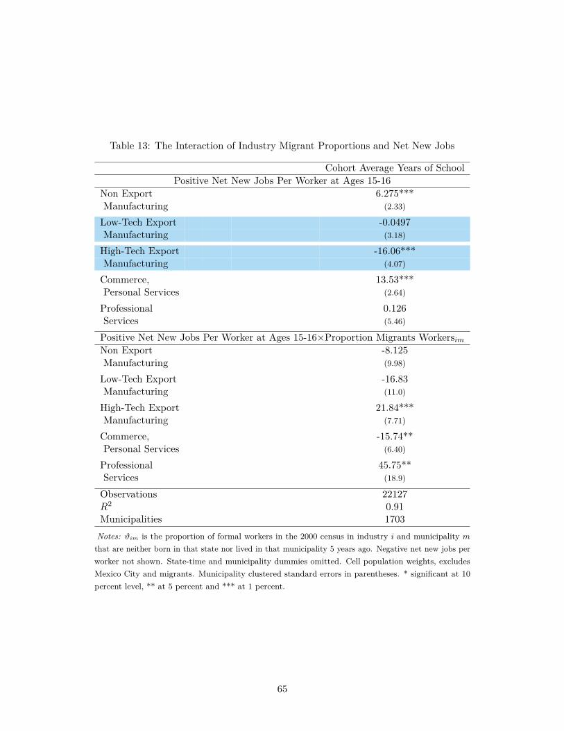
Table 13: The Interaction of Industry Migrant Proportions and Net New Jobs

Cohort Average Years of SchoolPositive Net New Jobs Per Worker at Ages 15-16

Non Export 6.275***Manufacturing (2.33)

Low-Tech Export -0.0497Manufacturing (3.18)

High-Tech Export -16.06***Manufacturing (4.07)

Commerce, 13.53***Personal Services (2.64)

Professional 0.126Services (5.46)

Positive Net New Jobs Per Worker at Ages 15-16×Proportion Migrants WorkersimNon Export -8.125Manufacturing (9.98)

Low-Tech Export -16.83Manufacturing (11.0)

High-Tech Export 21.84***Manufacturing (7.71)

Commerce, -15.74**Personal Services (6.40)

Professional 45.75**Services (18.9)

Observations 22127R2 0.91Municipalities 1703

Notes: ϑim is the proportion of formal workers in the 2000 census in industry i and municipality mthat are neither born in that state nor lived in that municipality 5 years ago. Negative net new jobs perworker not shown. State-time and municipality dummies omitted. Cell population weights, excludesMexico City and migrants. Municipality clustered standard errors in parentheses. * significant at 10percent level, ** at 5 percent and *** at 1 percent.

65