working for female manager: gender hierarchy in the workplace
TRANSCRIPT

1
Working for Female Manager:
Gender Hierarchy in the Workplace*
By
Illoong Kwon Eva Meyersson M. Milgrom
State University of New York
at Albany
Stanford University
April 2009
VERY PRELIMINARY AND INCOMPLETE
(DO NOT QUOTE WITHOUT PERMISSION OF AUTHORS)
Comments are Welcome.
Abstract
This paper analyzes how the number of women (or men) at top managerial positions affects
other male or female workers in the workplace. Despite growing gender quota policies, either
explicit or implicit, for top managerial positions in many organizations, the effects of such
policies on other female or male workers are largely unexplored. Using personnel data from
more than four hundred mergers and acquisitions in Sweden, we find that (i) when men face
more female managers after M&A, they become more likely to quit; (ii) when female
workers face more female managers, they become less likely to quit; (iii) when male workers
face more male managers after M&A, they become less likely to quit; and (iv) when female
workers face more male managers after M&A, they don’t seem to care. The same gender
attraction is the strongest when one’s own gender is a minority. However, the opposite gender
aversion is the strongest when neither gender group strongly dominates the other.
* Corresponding author: Illoong Kwon, Department of Economics, State University of New York at Albany,
1400 Washington Ave., Albany, NY 12222. Email: [email protected]. Tel: (518) 442-4737.

2
1. Introduction
Women have made striking advances in higher education, labor market participation, and
wages. However, women are still severely underrepresented in top positions in corporations,
governments, and in academics1. For example, women held only 14.7% of all Fortune 500
board director positions in 2005, 16.3% of seats in the US Congress in 2007, and 20% of all
tenured faculty positions in Ivy League schools in 2003. Moreover, the growth of these
numbers has slowed down dramatically in the last several years2.
In response, there has been growing political and social pressure to promote gender
parity at top positions via explicit or implicit gender quotas. For example, since 1988,
Norway legislation requires a minimum of 40% of each gender in publicly appointed
committees, boards, and councils. More than 22 countries have passed similar laws in the last
decade3, and many corporations and non-profit organizations are explicitly pursuing gender
diversity at the top management. However, it is still unclear whether these policies will break
the glass ceiling and advance the careers of other women. For example, Bagues and Esteve-
Volart (2007) suggests that female managers may be less favorable to female workers.
Moreover, it is also unclear how these policies will affect male workers4.
In this paper, we investigate detailed personnel records of white-collar workers in
various corporations in Sweden, and study how women’s share in top positions affects the
career paths of other male and female workers in the company. In particular, we use mergers
and acquisitions (M&A) of corporations as a natural experiment. For example, suppose that a
1 See, for example, Connolly and Long (2007).
2 Catalysis Survey (2009) “Women in U.S. Management”, available from
www.catalyst.org/file/192/qt_women_in_us_management.pdf 3 For latest information, check http://www.quotaproject.org.
4 Recent studies have focused on the effectiveness of gender quota at top positions, and largely ignored the
effect of gender quota on lower ranked male or female workers. See, for example, Dahlerup and Freidenvall
(forthcoming) and Squires (2004).

3
firm with few women in top positions has acquired another firm with many women in top
positions. Then, workers in the acquiring firm will suddenly find relatively more women at
the top of their hierarchy in the newly merged company. Then, we study how the careers of
men and women in the merged firm respond to this change after the acquisition. In particular,
we study whether men and women in the merged firm become more likely to stay or to quit.
The related theoretical models are diverse, and the predictions are ambiguous. On
one hand, if top female managers favor other female workers (similarity attraction
paradigm5) or if female workers see top female managers as their role models (social identity
theory6), of if top female managers correct the biased stereotype of females as leaders (social
belief theory7), female workers will be less likely to quit in the newly merged company, and
their wages and ranks should advance faster, while male workers may become more likely to
quit. On the other hand if top female managers identify with male managers and turn less
favorable to other females (self-enhancement drive8), or if there are limited quotas for female
top managers (tournament theory9), or if top female managers impose lower social status or
relative deprivation on other women (social status theory10), female workers will be more
likely to quit11, while male workers may be less likely to quit.
An important advantage of our empirical approach is that M&A can generate
significant changes in women’s share in top positions, but that an M&A decision itself is
typically not driven by gender-related issues. Therefore, we can establish a possible causal
link between the changes in women’s share in top positions and the subsequent response of
other female or male workers without worrying about other compounding gender factors that
5 See, for example, Byrne (1971).
6 See, for example, Akerlof and Kranton (2000) 7 See, for example, Boldy, Wood, and Kashy (2001).
8 Also related to social identity theory. See, for example, Graves and Powell (1995).
9 For example, see Niederle and Vesterlund (2006).
10 For example, see Ridgeway and Balkwell (1997). 11 See Bagues and Esteve-Volart (2007) for related evidence.

4
could generate a spurious relationship12.
We find that when the number of top female managers within the same occupation
increases, female workers, on average, become less likely to quit (called same gender
attraction), while male workers become more likely to quit (called opposite gender aversion).
In other words, top female managers have a positive effect on females, but a negative effect
on males. This result is important for gender (managerial or political) policies such as gender
quotas, as it suggests that gender quotas may indeed help other female workers’ careers, but
can have the cost of negatively affecting male workers’ career.
More importantly, we find large heterogeneity across occupations, especially due to
the difference in average share of female workers. In occupations where female share is less
than 10% on average, the increase in the number of female top managers reduces the male
workers’ turnover rates. In other words, in occupations where female is a weak minority
group, male workers seem to welcome additional female top managers. However, in
occupations where female share is in between 10% and 50%, an additional female top
manager increases male workers’ turnover rates significantly. Thus, when female is a strong
minority, male workers seem to resist to additional female top managers. Interestingly, once
the average female share goes above 50%, an additional female top manager has relatively
small effect on male turnover rates. We find the similar patterns of non-monotonicity in the
response of female workers to male top managers but in much lesser degree13.
This heterogeneity is important for several reasons. First, it explains why the female
share at top positions has grown fast initially but slowed down rapidly in recent years14.
12 Outside lab experiments (e.g. Niederle and Vesterlund 2006), few studies have used natural experiments (e.g.
Joy and Lang 2007). See Bagues and Esteve-Volart (2007) for an exception. 13 Allmendinger and Hackman (1995) finds the similar non-monotonicity (called threshold effect) between
female share and group performance. However, he does not control for the endogeneity of female share, and
does not distinguish male and female responses. 14 Catalyst 2007 Census of Women Corporate Officers and Top Earners of the Fortune 500, available from (as
of 05-07-2009)

5
Initially, when women are a weak minority, male workers would not resist to top female
managers. But as the female share increases, male workers would resist to additional top
female managers, which would slow down the growth of female share at top positions.
Second, even though the patterns of the same gender attraction and the opposite
gender aversion are similar between male and female, we find that the same gender attraction
is much stronger for female workers, and the opposite gender aversion is much stronger for
male workers. These results suggest that gender quota or gender parity policies cannot be
considered in a general model of majority vs. minority relationship, and requires gender-
specific models.
Third, this heterogeneity may explain why previous studies (that have focused on a
single occupation) found different results from ours. For example, Bagues and Esteve-Volart
(2007) uses a random assignment of female evaluators to an evaluation committee as a
natural experiment, and show that female evaluators are relatively more favorable to male
candidates than to female candidates15. But female evaluators are a small minority in most
committees in their sample. Recall that we also find that when women are a weak minority,
male workers welcome top female managers, which is consistent with their results. But our
analysis shows that their results do not generalize to other occupations with larger female
share or to larger complex corporations.
2. Data and Measurement
2.1 Data
Our analysis is based on the Swedish employer–employee matched data. The data cover
http://www.catalyst.org/publication/13/2007-catalyst-census-of-women-corporate-officers-and-top-earners-of-
the-fortune-500 . 15 This effect is sometimes called as “queen bee syndrome”. Giuliano, Levine, and Leonard (2006) also find
similar results in race and age, based on a single US retail firm.

6
almost the entire population of white collar workers in the private sector of Sweden during
the period 1970-1990, excluding financial sectors and CEOs. For each worker, the data
contain annual information on wage, age, education, gender, geographic region, work-time
status, firm ID, plant ID, industry ID, occupation code, and rank. Because all the IDs are
unique, we can track each individual worker within and across firms and occupations
throughout his/her career.
The unique feature of this Swedish data is the BNT code. BNT code is a four-digit
code, where the first three digits (occupation code) describe types of tasks and the fourth
(rank code) describes the degree of skill16 needed to fulfill the tasks. The white-collar
workers’ occupations cover 51 three-digit occupation groups such as construction, personnel
work, or marketing. For more details, see appendix A and B. Within each occupation, the rank
code runs from 1 (lowest) to 7 (highest)17.
As described below, the occupation and rank codes served as the input to the
centralized wage negotiations, and were gathered and monitored both by The Swedish
Federation of Employers and the labor unions. Thus, the occupation classification is of very
high quality with minimal potential errors. Most importantly, the occupation and rank codes
are comparable cross firms. Thus, we can analyze workers’ promotion patterns even when a
worker changes firms.
From this data, we focus on the firms involved in mergers and acquisition. Our data
do not firms’ financial information. Therefore, we identify mergers and acquisition based on
the changes in workers’ firm IDs. That is, if more than 50% of workers change firm ID18, say
from A to B, and if the old firm ID, A, disappears from the data, then we say “B has
16 Rank also reflects the number of employees and type of skill needed for decisions at that level.
17 Not all occupations span the entire 7 ranks, some start higher and some do not have the top ranks. For more
details, see appendix B. 18 Even when we require more than 90% of workers to change firm ID, there is very little change in our results.

7
acquired A”. We also refer to B as ‘acquirer’ and to A as ‘acquired’. We also restrict our
attention to firms with more than ten white-collar workers19. There are only a few clearly
identified merger cases where more than 50% of workers from both firm A and B move to a
new firm C, and firm A and B disappear. Therefore, we focus on clearly identified acquisition
cases only.20
This sample contains 443 acquisitions cases and 186,679 workers. Table 1 shows the
summary statistics of selected variables. Firm size is measured by the number of white-collar
workers, and it shows that acquiring firms are, on average, much larger than acquired firms.
The average ratio of acquired to acquirer firm size is 0.61, but there are large variations. The
wage is measured by monthly total compensation in 1970 Kronor. The wage of the acquiring
firms is slightly larger than that of acquired firm, but the difference can be mostly explained
by the fact that acquired firms have more highly-ranked positions.
[Table 1 here]
Status measures the relative ranking of each worker’s wage within his/her firm, where
0 is the lowest and 1 is the highest. Note that the average status of female is very similar
between acquiring and acquired firms. In fact, most other characteristics such as rank, age,
and part time ratio of female workers are very similar between acquiring and acquired firms.
This is important to note because our analyses will be based on the assumption that
acquisition decision is independent of gender aspects of the firms.
19 Focusing on firms with more than 100 white-collar workers does not change the qualitative results of the
paper. 20 Some firms are involved in more than one M&A during our sample period. Excluding M&As where the same
firm is involved in more than one M&A within 6 years does not change our qualitative results.

8
2.2 Institution
Beginning in 1966, wage setting for most private sector white collar workers in Sweden was
determined through negotiations between the Swedish Employers' Confederation (SAF) and
PTK, the main cartel for the private sector white collar union. After 1983, the central wage
bargaining system started to dissolve despite the government’s attempts to save it. For the
vast majority of all employees after 1988, wages were determined by industry- and plant-
level bargaining (Calmfors and Forslund 1990), while local plant unions continued to
represent workers. The occupation codes (called BNT code) were developed to facilitate the
wage negotiation. One of the goals was to pay the same wages for the same tasks, resulting in
wage compression within each occupation.
However, in practice, there existed significant wage variations within an occupation.
As Figure 1 shows, the highest-paid workers in a given rank often received larger wages than
the lowest-paid workers in a rank above. Also, the wage variation increases with ranks. Such
patterns are consistent with those observed in US firms. (see Baker et al. 1994, Kwon 2006)
[Figure 1 here]
Employers are also allowed to decide autonomously when it comes to hiring and
promotion. But firing workers is strictly regulated by law and is monitored by the labor
union.21
2.3 Gender Gap in Wages and Promotions
As a general background, we first describe gender gaps in wages and promotions briefly.
Table 2 shows a series of wage regressions with and without controlling for occupations and
21 For more details on the data and institution, see Kwon and Meyersson Milgrom (2006).

9
ranks. The dependent variable is the log of monthly total payment in 1970 Kronor. For these
regressions, we use all the white-collar workers (including those who are not involved in
acquisitions) in our data between 1986 and 198922.
[Table 2 here]
Column [1] shows that on average, female workers receive 39.6% lower wages than
male. However, once we control for occupation and rank, the gender wage gap reduces to
7.4%. Note that comparison between column [3] and [4] shows that ‘rank within occupation’
explains 10% differences in wages between two genders. It implies that women receive lower
averages wages than male because they are mostly placed in lower ranks, suggesting the
existence of potential ‘glass ceiling’ for women (see Meyersson Milgrom et al. 2001 for more
details).
Figure 1 shows that female represents about 30% of white-collar workers and that its
share has been slowly increasing.
[Figure 1 here]
However, Figure 2 shows that women are severely under-represented at higher ranks.
On average, at the highest rank (rank=7), female share is only 1.15%, while at the lowest rank
(rank=1), female share is 78%.
[Figure 2 here]
22 Using other time periods does not change our results.

10
Furthermore, Figure 3 shows that women’s shares at higher ranks have not increased
significantly during the period 1970-1990.
[Figure 3 here]
To investigate the ‘glass-ceiling’, we also look at the first-time labor market entrants
and analyzed their promotion patterns.
In Table 3, we construct rank transition matrix between the time of labor market
entry and ten years later. We constructed the matrices for each labor market entry cohort
between 1971 and 1980, and took the average.
[Table 3 here]
For example, if we focus on workers who started at rank 4, 34.97% of male have
moved up to rank 5 after 10 years, but only 26.73% of female have moved up to rank 5. Also,
9.02% of male moved up to rank 6, but only 3.58% of female moved up rank 6.
Table 4 shows the gender gap in the number of promotions within ten years since the
first labor market entry, controlling for education, starting occupation and rank. Column [1]
shows that in raw average, female has 0.1 times less promotions than male. However, once
we control for individual characteristics, especially the starting occupation and rank, female
has 0.57 times less promotions than male during the first ten years of their career. Given that
there are only seven ranks, this difference is economically significant.
[Table 4 here]

11
It is interesting to note that unlike gender wage gap, gender promotion gap increases
as we control for more individual characteristics. This is partly explained by the fact that
women tend to start at lower ranks where they have more room to get promoted.
Overall, we find that men and women receive similar wages within the same
occupation and rank, but women, on average, start their career at lower ranks and get
promoted more slowly than men. Especially, women’s representation at the top rank is
minimal. Therefore, women at top rank in this period can signify an important role model for
other women.
2.4 Acquisitions
As discussed earlier, we use acquisitions as a natural experiment, and study how the changes
in gender hierarchical structure during an acquisition affect female (or male) workers’ careers.
Thus, for our analysis, it is important that acquisition decisions are independent of gender
aspects of a company such as female share, or female status.
Table 5 shows that after controlling for firm size, primary industry, and primary
occupation of each firm23, the correlations between acquiring and acquired firms in gender
share and status are quite small. For example, correlation in overall female share is 20%, and
the correlation in average female status (=relative ranking of wages) is only 5.8%. Though
the correlation in female share at top rank is relatively large, it is mostly because female share
at the top ranks is zero for most firms. Thus, if one of two merged firms has some female at
the top ranks, it generates the negative correlation.
[Table 5 here]
23 We first regress, for example, female share on firm size, primary industry and occupation, then measure the
correlation of residuals between acquiring and acquired firms.

12
Therefore, it appears that an acquirer does not specifically look for a firm with
smaller (or larger) female share or a firm where women ranked relatively higher (or lower)
than men. Moreover, in our main analyses, we control for the gender compositions within
firm and within occupation between two merging firms. Then, a remaining concern is
whether the number of female at top managerial positions affects the merger decision.
However, it appears highly unlikely that a firm would merge with another firm because there
are more top female managers in the other firm, when the firm can simply hire new female
managers.
Another potential problem of using acquisition as a natural experiment is that
acquisitions are quite heterogeneous. Firms may acquire very similar firms in another
geographic market for its market expansion. Or firms may acquire their competitors in the
same market to increase their market power. Or firms may acquire very different firms for
complementarity or for business line expansions.
In order to classify different types of acquisitions, we construct a distance measure
between two firms in various aspects. The distance is measured by 1 – uncentered correlation,
as proposed by Jaffe (1986). For example, to measure the distance in occupation structure, we
construct a vector of occupation shares for an acquired firm, fi=(s1i,, s2i, …, s54i) where ski is
occupation k’s share in firm i (in terms of number of workers)24. Then, we construct the same
vector for its acquiring firm j, fj. Then, the distance in occupation structure is measured as
. This distance measure is zero if the composition of occupation is the same between
the two firms, and is one if two firms do not share any occupation.
24 We used 54 different occupations, 44 different industries, 24 different counties, 9 different education codes, 6
different age groups (11-20, 21-30, etc.), 7 rank codes, 2 gender codes, and 2 part time codes.

13
[Figure 4 here]
Figure 4 shows the histogram of each distance measures for 436 acquisitions in our
sample. The histogram for the distance in occupation structure shows large variations. In
other words, some firms are very close in terms of occupation structure, some firms are semi-
close, and some firms are completely different in occupation structure. On the other hand, if
we look at the distance in industry structure, and county location, firms are either close or far
way. Firms are always similar in most other dimensions25. Therefore, we classify acquisitions
as shown in Table 6.
[Table 6 here]
For example, if the acquired firm is similar in occupation and industry structures, and
in the same region, we call it as a horizontal merger. Also, as they are similar, we expect that
workers and business functions of two firms are substitutable. This classification is
admittedly arbitrary. However, this classification can give us some sense of whether our
results depend on different types of acquisition.
2.5 Changes in Gender Hierarchy
We measure gender hierarchy in the workplace in two ways: (i) the number of female (or
male) managers at the highest rank within a firm regardless of their occupations (henceforth
simply ‘within firm’) and (ii) the number of female (or male) managers at the highest rank
within the same occupation as a worker’s (henceforth simply ‘within occupation’). For
example, female (and male) workers in the marketing department may care the gender of
25 The variation in the rank distance can be mostly explained by the difference in size.

14
both the top managers within the marketing department (i.e. same occupation) and the top
managers within the firm as a whole.
Our analysis focuses on how the changes in female (and male) top managers affect
female (or male) workers’ turnover behaviors after an acquisition. However, for those who
quit during an acquisition, we don’t observe the number of their top managers after the
acquisition even though they are the ones who may respond to the changes most sensitively.
Moreover, the actual changes in the number of top managers can be correlated with other
structural changes during an acquisition.
Therefore, we use expected changes in the number of top managers instead of actual
changes. More specifically, we merge an acquiring firm’s and the acquired firm’s data right
before an acquisition and treat them as a single firm. Then, for each worker, we measure, for
example, the number of female at the top rank. We call this as expected post-merger number
of female at the top rank. The difference between the expected post-merger and actual pre-
merger number of female at the top rank is called the expected change in the number of
female at the top rank.26
[Table 7 here]
Table 7 shows an example of how expected post-merger measures are computed. In
this example, between the two firms, the top rank (within firm) is rank 5. Before the
acquisition, the acquiring firm has one female at the top rank, but the acquired firm has no
female at the top rank. If we merge the data between the two firms, then workers in the
acquired firm would also have one female at the top rank (worker 3). Therefore, the expected-
post merger number of female at the top rank changes from zero to one for worker 4 and 5.
26 For more details on these measures, see Kwon and Meyersson Milgrom (2007).

15
Other measures are computed in a similar way. We repeat the same computation for each
occupation to construct ‘within occupation’ measures.
Table 8 shows the summary statistics of expected changes in female hierarchy both
within firm and within occupation. As discussed above, for an average worker, the number of
female at top rank within his/her firm is very small. As a result, it does not change much even
with acquisitions. Therefore, later, we will use a dummy variable for whether the number of
female at top rank has increased or not. The number of female at one rank above is relatively
large, especially for female. It suggests that women tend to work for women. The changes in
the share of female or relative ranking of wages can be either positive or negative. Therefore,
the average is close to zero. However, note the relatively large standard deviation.
[Table 8 here]
2.6 Turnovers
We focus on how the changes in female hierarchy affect workers’ firm turnover decisions. If,
for example, the number of female at top rank decreases female turnover rates, we infer that
female at top rank raises other female workers’ (expected) utility.
The advantage of this approach is that we can infer workers’ preference from their
behavior without relying on often-problematic survey responses. Also, unlike other behavior,
such as consumption, the turnover decision does not rely upon an assumption on how the
changes in gender hierarchy affect marginal utility of workers.
The disadvantage of this approach is that some workers may get fired during
acquisitions, and that it is difficult to distinguish empirically between voluntary and
involuntary turnovers. In Sweden, however, it is generally difficult for firms to fire workers

16
without consent from labor union. Thus, we expect that the number of involuntary turnovers
would be small.
The average turnover rate is 12.4% for acquiring firms and 15.4% for acquired firms,
while the average turnover rate for all the firms (including those not involved in acquisitions)
in our full data is 14%. In other words, compared with an average firm, acquiring firms have
lower turnover rates, but acquired firms have higher turnover rates27. Thus, there is a concern
that some workers in acquired firms may get systematically fired during acquisitions. Table 9
confirms the same pattern using turnover regressions using 20% random sample of full data.
[Table 9]
For those who change firms, we also check how their wages have changed. If
workers got fired involuntarily, one can expect that they will have lower wages in another
firm than those who quit voluntarily. In Table 10, for those change firms only, we regress the
change in real wages on various individual and firm characteristics.
[Table 10]
As suspected, those who quit from acquired firms have much lower wage increase
than the average, while those who quit from acquiring firms have similar wage increase to the
average workers. Therefore, while most quits from acquiring firms are voluntary, most quits
from acquired firms appear to be involuntary.
27 Turnover regressions controlling for individual and firm characteristics yield the same results, and not
reported.

17
We address this problem in two ways. First, whenever possible, we check whether
our results are robust when we use the acquiring firms only. Second, we classify turnovers as
involuntary if (i) real wage falls from turnovers or (ii) real wage growth rate falls from
turnovers. Though none of these definitions are perfect, if our results are robust to various
definitions of involuntary turnovers, it is unlikely that involuntary turnovers from structural
changes of M&As are driving our results.
3. Gender Hierarchy and Turnover
We are now ready to study how the expected changes in the number of female (or male)
managers at top ranks affect other female (or male) workers’ turnover decision. Recall that
the top rank within firm is defined as the highest rank within an acquiring firm and an
acquired firm combined right before a merger. Thus, one firm may not have the top rank
before the acquisition, and that the top rank may differ across different acquisitions. We also
measure the top rank within occupation for each worker by the highest rank in the same
occupation within an acquiring firm and an acquired firm combined.
[Table 11 here]
In Table 11, we estimate the effect of expected changes in the number male/female
top managers on workers’ turnover decision within three years after acquisitions, controlling
for various individual and firm characteristics right before acquisitions, including pre-merger
number of male/female top managers both within firm and within occupation, acquired
dummy, age, age squared, part time dummy, firm size, firm size squared, real wage, firm size
change, occupation size change, ratio of workers who change regional code during

18
acquisition, female share within firm and within occupation, changes in female shares,
dummy variables for rank, occupation, industry, county, and year.
3.1 Female (or Male) Managers at Top Rank within Firm
From Table 11 column [1] and [2], when the expected number of male managers at a top rank
within firm increases, both male and female workers become more likely to quit. The same
pattern emerges even when the expected number of female managers at a top rank within firm
increases.
One explanation is that the increased number of male or female managers at top rank
implies less chance of future promotions or the decreased status of other workers, which can
induce larger turnover rates.
Note that the coefficients are almost the same between male and female workers. In
other words, there is no gender difference when it comes to the way workers respond to the
number of male (or female) managers at the top rank within firm. Later, we confirm this
result more explicitly using difference-in-difference estimation.
3.2 Female (or Male) Managers at Top Rank within Occupation
With respect to the expected changes in the number of top female or male managers within
the same occupation, however, column [3] and [4] show clear difference between male and
female. When the expected number of male managers at a top rank within the same
occupation increases, male workers become less likely to quit, but female workers become
more likely to quit. Similarly, when the expected number of female managers at a top rank
within the same occupation increases, male workers become more likely to quit, but female
workers become less likely to quit. Column [5] and [6] show the same pattern when we
control for both top rank within firm and top rank within occupation.

19
From column [5] and [6], both male and female workers seem to equally like to have
more same-gender top managers within the same occupation (called same gender attraction).
However, both male and female workers do not like to have the opposite gender top
managers within the same occupation (called opposite gender aversion). It is interesting to
note that opposite gender aversion is particularly strong for male workers.
These results are noteworthy for several reasons. First, these results differ from the
findings of recent studies that are based on a single firm or a single occupation. For example,
Bagues and Esteve-Volart (2007) finds that female evaluators are relatively more favorable to
men than to women, which would at least partially undermine a goal of gender quota policy.
In a related study, Giuliano, Levine, and Leonard (2006) find that black (young) managers are
relatively more favorable to white (older) workers. In contrast, we find that on average,
female workers do prefer having more female top managers and less male managers. Our
results do not necessarily mean that female top managers are relatively more favorable to
female workers. Instead, our results imply that the positive effects of having more female top
managers on female workers (such as aspiration, role model) dominate other possible
negative effects.
Second, the gender policies, including gender quota, typically do not explicitly
consider its effect on male workers. However, our results show that the largest effect of
adding an additional top female manager would be the increased quits by the male workers.
Therefore, such negative effect on male workers’ careers should be considered in the gender
policy decision process.
Third, female workers, on average, do not respond to the increased number of male
top managers within the same occupation. One explanation is that female workers may take
male top managers for granted as a social norm. Later we show that in occupations where
female share is large (that is, having female top managers is a norm), female workers do

20
respond negatively (i.e. quit more) to the increased number of male top managers within
occupation.
Finally, as we show in next subsection, these different responses between male and
female workers imply that our qualitative results would be robust even in difference-in-
difference (between before and after merger and between male and female workers)
estimation. In other words, our qualitative results are robust to unobserved M&A
characteristics or firm characteristics.
3.3 Robustness
■ Acquiring vs. Acquired Company
Workers’ turnover in acquired firms may not be voluntary, as discussed above. Also, workers
in acquiring firms may respond more strongly to the top managers from acquired firms, if
they consider acquiring firms as a higher-status group. Therefore, we repeat the same analysis
for acquiring firms and acquired firms separately.
[Table 12 here]
Table 12 shows that within acquiring firms only, we find essentially the same
patterns as before. However, for acquired firms, the changes in the number of top managers
within occupation, regardless of its gender, are not significant. Moreover, the changes in the
number of top female managers within firm have very different effects.
It is not clear whether this difference between acquiring firms and acquired firms is
due to the fact that many turnovers within acquired firms are involuntary or to the fact that
workers in acquired firms feel less secure about their identity. This is an interesting topic for

21
future research but outside the scope of this paper. Instead, we will focus on either all firms or
acquiring firms only.
■ Alternative Measure
Given that the number of female at top rank is very small, the expected changes in the
number of female, especially within firm, are typically either zero or one. Therefore, in Table
12A, we use a dummy variable (equal to one if the expected change is positive) for the
expected changes. Table 12A shows essentially the same qualitative results as Table 12. One
difference is that female workers’ response to the expected changes in the number of male
managers at top rank within occupation becomes statistically significant. In other words,
female workers also become more likely to quit when the opposite gender managers at top
rank within occupation increases (= opposite gender aversion).
[Table 12A here]
■ Involuntary Turnovers
We can infer workers’ preference from their voluntary turnover decisions. However, during
an M&A, workers may get dismissed involuntarily due to structural changes from M&A. For
example, some top managers may get dismissed because they have become redundant. Note
that these structural changes should affect both male and female workers. Therefore,
involuntary turnovers or structural changes during M&As don’t necessarily explain different
responses by male and female workers.
Still, in order to check the robustness of our results, we classify turnovers as
involuntary if (i) real wage falls from turnovers, or (ii) real wage growth rate falls from

22
turnovers compared with those who are remaining in the firm. Then, in Table 13, we estimate
the probit model for voluntary turnovers only.
[Table 13 here]
Table 13 shows that the qualitative results from all turnovers (see Table 11) do not
change even when we omit involuntary turnovers.
■ Types of M&A
As discussed above, M&As are heterogeneous in various dimensions. Thus, in Table 14 we
control for different types of M&As. First, we control M&A types according to the
classification in Table 6. Then, we control for all 8 distance measures (shown in Figure 4).
[Table 14 here]
The first two columns in Table 14 show that different types of M&A have different
effect on workers’ turnover rates. For example, ‘growth’ type increases workers’ turnover
rates, but ‘horizontal merger’ decreases workers’ turnover rates28. In the third and fourth
columns, we control for distance measures between acquiring and acquired firms in various
dimensions.
In all cases, however, note that the qualitative effect of the expected changes in top
male/female managers within occupation on male and female workers’ turnover rates remain
the same. In fact, the estimates become statistically more significant.
28 This difference is not the primary focus of this paper, but is certainly interesting for future research.

23
■ Difference-in-Difference
So far, we have estimated the probit models separately for male and female. The difference
between male and female is easy to observe from our results. However, our estimates of the
marginal effect (dP/dx) for male and female are evaluated at different points. Thus,
technically, the direct comparison of the coefficients between male and female is potentially
biased. Thus, in Table 15, we estimate a difference-in-difference (between before and after
merger and between male and female) model more explicitly using interaction terms between
the changes in the number of male/female top managers and female dummy variable.
[Table 15 here]
Column [1] of Table 15 shows that as expected, when the number of top male or female
managers within firm increases, there is no (either statistically or economically) differential
effect on male and female workers. However, when the number of top male managers within
occupation increases, female workers become more (relative to male) likely to quit. Also,
when the number of top female managers within occupation increases, female workers
become relatively less likely to quit.
These results do not change even when we control different types of M&A interacted
with female dummy variable, as shown in column [2]. Since it is not always straightforward
to interpret interaction terms in a probit model, we also estimate a linear probability model in
column [3]. The results remain the same.
In column [4] and [5], we estimate the model separately for acquiring firms and
acquired firms. Like before, the results remain the same for acquiring firms, but not for
acquired firms.

24
In summary, our results are largely robust to various specifications and measures.
Note, however, that the results in this section measure the average effect for male and female
workers. As we show in next section, it turns out that the average effect does not apply to all
workers or occupations.
4. Majority vs. Minority
There exists large heterogeneity in the share of female workers across occupations. For
example, in production management (BNT codes 100, 110, 120, 140, and 160), the average
share of female workers is less than 3%. However, in personnel work (BNT codes 600, 620,
and 640) and office services (BNT codes 970 and 985), the average share of female workers
is larger than 60%.
[Table 16 here]
Therefore, in Table 16, we first classify occupations into three groups: (i) the share of
female workers is less than 10%, (ii) the share of female workers is between 10% and 50%,
and (iii) the share of female workers is larger than 50%, and estimate our model separately
for each group. Note that in the first group, women are a weak minority. In the second group,
women are a strong minority, and in the third group, women are a majority. In this section,
we primarily focus on the effect of the (expected) change in top male/female managers within
occupation.

25
4.1 Same Gender Attraction
In the previous section, we show that on average, both male and female workers exhibit same
gender attraction. In other words, when the number of the same gender top managers
increases, workers become less likely to quit.
Table 16 shows that this same gender attraction is particularly strong for female
workers, and that it is the strongest when one’s own gender is a (weak) minority. More
specifically, from the fourth row and female columns in Table 16, an additional increase in
the number of female top managers within occupation reduces female workers’ turnover rates
by 18.9, 8.7, and 0.5 percentage point, in occupations where the female share is less than 10%,
between 10% and 50%, and larger than 50%, respectively.
For male workers (from the third row and male columns in Table 16), the same
gender attraction is much smaller, and is not monotonic to the female share. However, it is
still true that the largest same gender attraction is observed in occupations where female share
is larger than 50% (i.e. male share is less than 50%). Figure 5 illustrates these results clearly.
[Figure 5 here]
It is worth emphasizing that in occupations where women are a weak minority, an
additional female top manager has very large (positive) effect on female workers. Even
though this effect is not statistically significant (because there are too few top female
managers in these occupations), it suggests that a gender quota policy can have significant
effect on female workers in occupations where women are traditionally a weak minority.

26
4.2 Opposite Gender Aversion
In the previous section, we show that both male and female exhibit opposite gender aversion.
In other words, when the number of opposite gender top managers increases, workers become
more likely to quit. Table 16 shows that this opposite gender aversion is particularly strong
for male workers, and that it is the strongest when the female share is between 10% and 50%
(or when women are a strong minority).
More specifically, from the fourth row and male columns of Table 16, an additional
female top manager within occupation increases male workers’ turnover rates by -17, 14.5
and 2.8 percentage point in occupations where the female share is less than 10%, between
10% and 50%, and larger than 50%, respectively.
For female workers (from the third row and female columns), an additional male top
manager within occupation increases female workers turnover rates only in occupations
where female share is between 10% and 50%. These results can be also seen in Figure 6.
[Figure 6 here]
It is interesting to note that in occupations where female share is less than 10%, male
workers do not show the opposite gender aversion. In fact, in these occupations where
women are a weak minority, if the number of female top managers within occupation
increases, male workers’ turnover rates decrease as if they welcome female top managers.
However, male workers’ response changes completely in occupations where women are a
strong minority, as they become more likely to quit when the number of female top managers
increases. Interestingly, male workers’ opposite gender aversion becomes smaller when

27
women are a majority. Female workers show the same non-monotonicity but in much lesser
degree.
4.3 Discussion
This heterogeneity of the same gender attraction and the opposite gender aversion provides
several important implications. First, it can explain why the growth of female share at top
managerial positions in U.S. has slowed down recently. For example, Figure 7 shows that the
women’s share in the board or in corporate officer positions in fortune 500 firms has grown
steadily in 1990s. However, as the women’s share passes over 10%, the growth rate has
slowed down significantly. In fact, the women’s share in corporate officer positions has
decreased after 2005.
[Figure 7 here]
Our results show that when female share is less than 10%, male workers welcome
(and do not resist to) an additional female top managers. Also, female workers respond very
positively (by reducing their turnover rates) to an additional female top manager. These
findings can explain the steady growth of the share of women at top managerial positions in
1990s when the women’s share at top managerial position was less than 10%.
However, our results suggest that when female share is between 10% and 50%, male
workers would strongly resist to an additional female top managers, while the positive effect
of an additional female top managers for female workers decreases. These findings provide a
potential explanation why the growth of female share at top managerial positions has slowed
down after 2000 when the women’s share at top managerial position passed over 12%.

28
Second, from the policy perspective, if the goal is to achieve gender parity at top
managerial positions, our results suggest that a gender quota policy may be necessary.
Without a gender quota policy, women share at top managerial positions may not increase
due to male resistance. On the other hand, as discussed above, our results show that the
gender quota policy would have potentially negative effect on male workers’ careers.
Therefore, such costs must be taken into account in the policy decision process.
Third, as shown in Figure 5 and 6, even though the general relationship between
same gender attraction (or opposite gender aversion) and the share of one’s own gender is
similar between male and female workers, there exist clear asymmetry between male and
female. The same gender attraction is much stronger for female workers. And the opposite
gender aversion is much stronger for male workers. These results imply that gender issues,
such as gender quota or gender parity policies, cannot be fully explained by a general model
of majority vs. minority, and require gender-specific models.
5. Conclusion
To be written.

29
Reference
Akerlof, George and Rachel E. Kranton, 2000, “Economics and Identity,” Quarterly Journal of
Economics, v. 115 (3), pp. 715-33
Allmendinger, Jutta, and Richard J. Hackman, 1995, “The More, the Better? A Four-Nation Study of
the Inclusion of Women in Symphony Orchestras,” Social Forces, 74(2): pp. 423-460.
Athey, Susan, Christopher Avery, and Peter Aernsky, 2000, “Mentoring and Diversity,” American
Economic Review, v 90 (4), pp. 765-86
Bagues F. Manuel and Berta Esteve-Volart, 2007, “Can gender parity break the glass ceiling?
Evidence from a repeated randomized experiment,” mimeo, Universidad Carlos III
Bertrand, Marianne and Kevin F. Hallock, 2001, “The Gender Gap in Top Corporate Jobs,” Industrial
and Labor Relations Review, v. 55 (1), pp. 3-21
Boldry, J.,Wood,W., & Kashy, D. A., 2001, “Gender stereotypes and the evaluation of men and
women in military training,” Journal of Social Issues, 57, pp. 689–705.
Bose E. Christine, Peter H. Rossi, 1983, “Gender and Jobs: Prestige Standings of Occupation as
Affected by Gender,” American Sociological Review, v 48 (3), pp. 316-330
Byrne, D., 1971, The Attraction Paradigm (New York: Academic Press)
Cohen, Lisa E, Joseph P. Broschak, Heather A. Haveman, 2000, “An Then There Were More? The
Effect of Organizational Sex Composition on the Hiring and Promotion of Managers,’ American
Sociological Review, v 63
Connolly Sara and Susan Long, 2007, “Women in science – fullfillment or frustration? Evidence from
the UK”, mimeo, University of East Anglia
Dahlerup, Drude and Lenita Freidenvall, forthcoming, “Quotas as a ‘Fast Track’ to Equal
Representation for Women. Why Scandinavian is no longer the model,” International Feminist Journal
of Politics
Dahlerup, Drude, 2006, Women, Quotas and Politics (London: Routledge)
Dufwenberg, Martin and Astri Muren, 2005, “Gender Composition in Teams,” Journal of Games and
Economic Behavior, 30
Eagly, Allice H. and Steven J. Karau, 1992, “Role Congruity Theory of Prejudice Toward Female
Leaders,” Psychological Review, v. 3, pp. 573-589
Ely, Robin J., 1995, “The Power in Demography: Women’s Social Constructions of Gender Identity at
Work,” Academy of Management Journal, v. 38 (3), pp. 589-634
Giuliano, Laura, David I. Levine, and Jonathan Leonard, 2006, “Do Race, Age, and Gender
Differences Affect Manager-Employee Relations?” Institute for Research on Labor and Employment
Working Paper

30
Graves, L. M. and G. N. Powell, 1995, “The Effect of Sex Similarity on Recruiters’ Evaluations of Actual Applicants: A Test of the Similarity-Attraction Paradigm,” Personnel Psychology, v 48 (1), pp.
243-61
Hamermesh, Daniel, 1994, “Beauty and the Labor Market,” American Economic Review
Heilman, Madeline, 2001, “Description and Prescription: How Gender Stereotypes Prevent Women’s
Ascent Up the Organizational Ladder,” Journal of Social Issues, v. 4, pp. 657-674
Heilman, M. E., Martell, R. F., and M.C. Simon, 1988, “The vagaries of sex bias: Conditions
regulating the undervaluation, equivaluation and overvaluation of female job applicants,”
Organizational Behavior and Human Decision Processes, 41, pp. 98-110
Joy, Lois and Sarah Lang, 2007, “Do Women in Top Corporate Management and Governance Help
Women to Advance?”, mimeo , Catalyst
Kwon, Illoong and Eva Meyersson Milgrom, 2006, “Boundary of Internal Labor Market: Occupation
vs. Firm,” mimeo, SUNY Albany
Kwon, Illoong and Eva Myersson Milgrom, 2007, “Status, Relative Pay, and Wage Growth: Evidence
from M&As,” mimeo, SUNY Albany
Lazear, Edward P. and Sherwin Rosen, 1990, “Male-Female Wage Differentials in Job Ladders,”
Journal of Labour Economics, v. 8 (1).
Lavy, Victor, 2004, “Do Gender Stereotypes Reduce Girls’ Human Capital Outcomes? Evidence from
a Natural Experiment, mimeo, Hebrew University of Jerusalem
Madden, T. R., 1987, Women versus women: The uncivil business war. New York: AMACOM.
Meyersson Milgrom, Eva M., Petersen, T. and V. Snartland. 2001. “Equal Pay for Equal Work? Evidence from Sweden and Comparison with Norway and the U.S.” Scandinavian Journal of
Economics
Niederle Muriel and Lise Vesterlund, 2006, “Do Women Shy Away From Competition? Do Men
Compete Too Much?,” Quarterly Journal of Economics forthcoming.
Powell, G. N. , 1990, “One more time: do female and male managers differ?,” Academy of Management Executive, 4, pp. 68–75.
Ridgeway L. Cecilia and James W. Balkwell, 1997, “Group Processes and the Diffusion of Status Beliefs,” Social Psychology Quarterly, v 60 (1), pp.14-31
Squires, Judith, 2004, “Gender Quotas in Britain: A Fast Track to Equality,” mimeo, Stockholm
University

31
Appendix A Three-Digit Occupation Codes
BNT
Family
BNT
Code Levels
0 Administrative work
020 7 General analytical work
025 6 Secretarial work, typing and translation
060 6 Administrative efficiency improvement and development 070 6 Applied data processing, systems analysis and programming
075 7 Applied data processing operation
076 4 Key punching
1 Production Management
100 4 Administration of local plants and branches
110 5 Management of production, transportation and maintenance work
120 5 Work supervision within production, repairs, transportation and maintenance work
140 5 Work supervision within building and construction
160 4 Administration, production and work supervision within forestry, log
floating and timber scaling
2 Research and Development
200 6 Mathematical work and calculation methodology
210 7 Laboratory work
3 Construction and Design
310 7 Mechanical and electrical design engineering
320 6 Construction and construction programming 330 6 Architectural work
350 7 Design, drawing and decoration 380 4 Photography
381 2 Sound technology
4 Technical Methodology, Planning, Control, Service and Industrial
Preventive Health Care
400 6 Production engineering
410 7 Production planning
415 6 Traffic and transportation planning
440 7 Quality control
470 6 Technical service
480 5 Industrial, preventive health care, fire protection, security, industrial civil
defense
5 Communications, Library and Archival Work
550 5 Information work 560 5 Editorial work – publishing
570 4 Editorial work – technical information
590 6 Library, archives and documentation
6 Personnel Work 600 7 Personnel service
620 6 The planning of education, training and teaching

32
640 4 Medical care within industries
7 General Services
775 3 Restaurant work
8 Business and Trade 800 7 Marketing and sales
815 4 Sales within stores and department stores
825 4 Travel agency work
830 4 Sales at exhibitions, spare part depots etc.
835 3 Customer service
840 5 Tender calculation
850 5 Order processing
855 4 The internal processing of customer requests
860 5 Advertising 870 7 Buying
880 6 Management of inventory and sales
890 6 Shipping and freight services
9 Financial Work and Office Services
900 7 Financial administration 920 6 Management of housing and real estate
940 6 Auditing
970 4 Telephone work
985 6 Office services
986 1 Chauffeuring

33
Appendix B Sample Description of Four-Digit Occupation Codes
Occupation Family 1: Occupation # 120- Manufacturing, Repair, Maintenance, and Transportation 11% of 1988 sample
There is no rank 1 in this occupation.
Rank 2 (4% of occupation # 120 employees) - Assistant for unit; insures instructions are followed;
monitors processes
Rank 3 (46%) -In charge ofa unit of 15-35 people
Rank 4 (45%) - In charge of 30-90 people; does investigations of disruptions and injuries
Rank 5 (4%) - In charge of 90-180 people; manages more complicated tasks
Rank 6 (0.3%) - Manages 180 or more people
There is no rank 7 in this occupation.
Occupation Family 2: Occupation #310- Construction
10% of the 1988 sample Rank l (0.1%) - Cleans sketches; writes descriptions
Rank 2 (1%) - Does more advanced sketches
Rank 3 (12%) - Simple calculations regarding dimensions, materials, etc. Rank 4 (45%) - Chooses components; does more detailed sketches and descriptions; estimates costs
Rank 5 (32%) - Designs mechanical products and technical products; does investigations; has 3 or more
subordinates at lower Ranks
Rank 6 (8%) - Executes complex calculations; checks materials; leads construction work; has 3 or more
subordinates at rank 5
Rank 7 (1%) - Same as rank 6 plus has 2-5 rank 6 subordinates
Occupation Family 3: Occupation #800- Marketing and Sales
19% of 1988 sample Rank l (0.2%) - Telesales; expedites invoices; files
Rank 2 (6% ) - Puts together orders; distributes price and product information
Rank 3 (29%) - Seeks new clients for 1- 3 products; can sign orders; does market surveys Rank 4 (38%) - Sells more and more complex products; negotiates bigger orders; manages 3 or more
subordinates
Rank 5 (20%) - Manages budgets; develops products; manages 3 or more rank 4 workers
Rank 6 (7%) - Organizes, plans, and evaluates salesforce; does more advanced budgeting; manages 3 or
more rank 5 workers
Rank 7 (1 %) - Same as rank 6 plus 2-5 rank 6 subordinates
Occupation Family 4: Occupation #900- Financial Administration
5% of 1988 sample
Rank 1 (1% ) - Office work; bookkeeping; invoices; bank verification Rank 2 (7%) - Manages petty cash; calculates salaries
Rank 3 (18%) - More advanced accounting; 4-10 subordinates
Rank 4 (31 %) - Places liquid assets; manages lenders; evaluates credit ofbuyers; manages 3 or more rank
3 employees
Rank 5 (28%) - Financial planning; analyzes markets; manages portfolios; currency transfers; manages 3
or more rank 4 employees Rank 6 (12%) - Manages credits; plan routines within the organization; forward-looking budgeting;
manages 3 or more rank 5 employees
Rank 7 (2%) - Same as rank 6 plus 2-5 rank 6 subordinates

34
Table 1 Summary Statistics
total male female total male female
firm size 362.627 273.283 90.533 51.463 37.168 14.457
female ratio 0.302 0.282
wage 1532.499 1717.705 1054.538 1493.726 1661.137 1015.019
status 0.510 0.623 0.238 0.521 0.633 0.232
rank 3.322 3.715 2.380 3.279 3.630 2.349
age 40.955 42.247 37.446 40.964 42.442 36.753
part time 0.103 0.021 0.280 0.102 0.019 0.293
acquirer acquried
Note: Wage is a monthly total payment measured in 1970 Kronor. Status is measured as each worker’s
relative ranking of wages within a firm where zero is the lowest and one is the highest.

35
Table 2 Gender Wage Gap
(dependent variable = log(real wage))
[1] [2] [3] [4] [5]
female -0.396 -0.199 -0.177 -0.074 -0.065
(0.001)** (0.000)** (0.001)** (0.000)** (0.000)**
age 0.057 0.053 0.034 0.034
(0.000)** (0.000)** (0.000)** (0.000)**
age2 -0.001 -0.001 0 0
(0.000)** (0.000)** (0.000)** (0.000)**
tenure 0.018 0.018 0.008 0.009
(0.000)** (0.000)** (0.000)** (0.000)**
tenure2 -0.001 -0.001 0 0
(0.000)** (0.000)** (0.000)** (0.000)**
occupation no no yes yes yes
rank no no no yes yes
job no no no no yes
other controls no yes yes yes yes
Observations 1204643 1204643 1204643 1204643 1204643
R-squared 0.28 0.63 0.68 0.81 0.82
Standard errors in parentheses.
* significant at 5%; ** significant at 10%.
Note: Observations include only all the white-collar workers between 1987 and 1990. Tenure is
measured by the number of years since the first labor market entry. Occupation is the first-three digits
of BNT code, rank is the fourth digit of BNT code. Job is the full four digit BNT code. Other controls
include part time dummy, 8 education dummies, 44 industry dummies, 24 county dummies, and 4
year dummies.

36
Table 3 Transition Matrix between Starting Year and 10 Years Later
(Male)
starting
rank 1 2 3 4 5 6 7
1 10.77 29.01 36.82 20.29 2.97 0.14 0.00
2 0.85 20.80 37.04 33.56 7.15 0.56 0.04
3 0.14 2.66 35.87 44.75 14.55 1.90 0.12
4 0.03 0.70 7.38 47.02 34.97 9.02 0.87
5 0.00 0.28 2.04 12.64 54.60 26.76 3.68
6 0.00 0.12 0.82 3.94 19.64 62.54 12.94
7 0.00 0.00 0.42 2.16 11.10 25.63 60.69
rank after 10 years
(Female)
starting
rank 1 2 3 4 5 6 7
1 15.73 53.91 26.08 3.98 0.29 0.01 0.00
2 2.89 47.12 39.31 9.63 1.00 0.05 0.00
3 0.64 9.92 53.23 30.17 5.78 0.26 0.01
4 0.13 2.41 9.61 57.46 26.73 3.58 0.15
5 0.11 1.56 7.65 26.56 50.11 13.33 1.12
6 0.00 6.67 0.00 7.50 32.08 47.08 10.67
7 0.00 0.00 0.00 100.00 0.00 0.00 0.00
rank after 10 years (cross occupation)
Note: The table reads as follows. For example, for male, for those who started at rank 4, after 10 years,
7.38% fell to rank 3, 47.02% remains in rank 4, 34.97% moves up to rank 5, 9.02% moves up to rank 6, 0.87% moves up to rank 7. For each gender, transition matrices for each starting year from 1971
and 1980 are computed, and then averaged over years to produce these tables.

37
Table 4 Gender Promotion Gap
(dependent variable = number of promotions in the first ten years)
[1] [2] [3] [4] [5]
female -0.121 -0.139 -0.276 -0.578 -0.563
(0.004)** (0.005)** (0.006)** (0.006)** (0.006)**
age -0.082 -0.066 0.011 0.012
(0.002)** (0.002)** (0.002)** (0.002)**
age2 0.001 0.001 0 0
(0.000)** (0.000)** (0.000)** (0.000)**
occupation no no yes yes yes
rank no no no yes yes
job no no no no yes
other controls no yes yes yes yes
Observations 167664 167664 167664 167664 167664
R-squared 0 0.16 0.18 0.34 0.35 Standard errors in parentheses.
* significant at 5%; ** significant at 10%.
Note: Observations include only those who entered the dataset between 1971 and 1980, and those
who stay after 10 years. All the independent variables are measured at the time of entry. Other
controls include part time dummy, education dummies, industry dummies, county dummies, and year dummies.

38
Table 5 Correlations between Acquiring and Acquired Firms
Overall At Top RankAt Top Rank
within Occup.Within Firm Within Occup.
corr(acquiring, acquired) 0.200 -0.325 0.131 0.058 0.064
Female Share Female Status
Note: The correlations after controlling for firm size, firm size squared, primary industry dummy, and
primary occupation dummy.
Table 6 Classification of Acquisition
Occupation Industry Region Description Classification Complementarity
Similar Similar Similar Acquisition of Competitor Horizontal Merger -5
Similar Similar Different Regional Expansion Growth Merger -3
Different Similar Similar 5
Different Similar Different 3
Similar Different Similar Product Line Extension Growth Merger -3
Similar Different Different Product/Region Expansion Growth Merger -1
Different Different Similar 3
Different Different Different 0
Vertical Merger
Conglomerate Merger
Functional Extension
Business Line Expansion
Occupation: similar if occupation distance measure is less than 0.2, different otherwise.
Industry: similar if industry distance measure is less than 0.5, different otherwise. Region: similar if regional distance measure is less than 0.5, different otherwise.

39
Table 7 Computation of Expected Post-Merger Measures: An Example
firm worker gender rank wage
1 male 4 1500 1 1 1/1 1 1 2/2
2 female 4 1600 1 1 1/2 1 1 2/3
3 female 5 1800 1 . 2/2 1 . 3/3
4 male 3 1200 0 1 1/1 1 2 1/2
5 female 4 1300 0 0 1/1 1 1 1/3
Acquiring
Acquired
Pre-Merger Expected Post-MergerNumber of
Female at
Top Rank
Number of
Female at a
Rank above
Relative
Ranking
within Gender
Number of
Female at
Top Rank
Number of
Female at a
Rank above
Relative
Ranking
within Gender

40
Table 8 Changes in Female Hierarchy
Pre-Merger Expected Change Pre-Merger Expected Change
0.028 0.011 0.067 0.013
(0.189) (0.123) (0.317) (0.132)
0.269 0.087 0.637 0.045
(2.259) (1.695) (3.522) (2.566)
22.100 2.834 90.722 10.613
(48.680) (14.159) (110.541) (33.381)
5.846 0.035 26.976 -0.245
(10.232) (2.505) (21.874) (3.786)
0.499 0.000 0.503 0.000
(0.286) (0.029) (0.287) (0.038)
number of
observation142,176 44,503
Female
Number of Female
at Top Rank
Share of Female at
Top Rank (%)
Number of Female
at Rank above
Share of Female at
Rank above (%)
Relative Ranking
within Gender
Male
(a) Within Firm
Pre-Merger Expected Change Pre-Merger Expected Change
0.071 0.012 2.910 0.372
(0.765) (0.205) (6.732) (1.839)
1.056 0.083 32.775 0.851
(7.662) (2.930) (44.374) (10.034)
2.222 0.346 24.196 3.547
(13.188) (4.335) (45.342) (15.281)
3.990 0.035 53.370 0.002
(11.896) (2.728) (37.801) (5.987)
0.511 -0.002 0.527 -0.003
(0.289) (0.043) (0.291) (0.049)
number of
observation142,176 44,503
Share of Female at
Rank above (%)
Relative Ranking
within Gender
Male Female
Number of Female
at Top Rank
Share of Female at
Top Rank (%)
Number of Female
at Rank above
(b) Within Occupation
Note: Standard deviations are in parenthesis.

41
Table 9 Turnover Pattern: Probit Analysis
(dependent variable = 1 if quit)
[1] [2] [3]
all male female
age -0.027 -0.027 -0.023
(0.000)*** (0.001)*** (0.000)***
age_sq 0 0 0
(0.000)*** (0.000)*** (0.000)***
part time 0.033 0.102 0.019
(0.001)*** (0.004)*** (0.002)***
firm size 0 0 0
(0.000)*** (0.000)*** (0.000)***
firm size_sq 0 0 0
(0.000)** (0.000)** (0.000)*
acquirer -0.03 -0.031 -0.025
(0.005)*** (0.005)*** (0.008)***
acquired 0.871 0.877 0.856
(0.002)*** (0.002)*** (0.003)***
female -0.013
(0.001)***
Observations 1,283,996 902,656 381,320
Note: 20% random sample of full data (including those not involved in acquisitions) is used. Each
regression includes education, rank, occupation, industry, county, and year dummies.

42
Table 10 Wage Changes After Quit
(dependent variable = log(wage_new)-log(wage_old))
[1] [2] [3]
all male female
age -13.988 -23.312 -16.755
(1.321)*** (2.055)*** (1.739)***
age_sq 0.019 0.099 0.136
(0.017) (0.025)*** (0.023)***
part 300.552 301.648 280.949
(10.195)*** (27.510)*** (9.782)***
fsize 0.015 0.020 -0.003
(0.010) (0.011)* (0.008)
fsize2 -0.000 -0.000 -0.000
(0.000)* (0.000)** (0.000)
acquirer -0.749 -2.462 -10.609
(14.559) (18.287) (25.635)
acquired -55.019 -51.938 -42.908
(10.159)*** (12.081)*** (13.149)***
female -223.104
(7.652)***
Observations 92803 65356 27447
R-squared 0.13 0.14 0.12
Note: Among 20% random sample of full data, only those who change firms (including those not
involved in acquisitions) are used. Each regression includes education, rank, occupation, industry,
county, and year dummies.

43
Table 11 =umber of Female at Top Rank and Turnover: Probit Analysis
(dependent variable =1 if quit within three years after acquisitions)
Male Female Male Female Male Female
0.002 0.003 0.003 0.003
(0.000)*** (0.000)*** (0.000)*** (0.000)***
0.073 0.055 0.061 0.056
(0.012)*** (0.023)** (0.012)*** (0.024)**
-0.004 0.008 -0.005 0.003
(0.000)*** (0.002)*** (0.000)*** (0.002)
0.025 -0.001 0.025 -0.005
(0.009)*** (0.002) (0.009)*** (0.002)***
0.000 0.001 0.001 0.000
(0.000)*** (0.000)* (0.000)*** (0.000)
-0.026 -0.069 -0.027 -0.067
(0.008)*** (0.012)*** (0.008)*** (0.012)***
-0.001 -0.001 -0.001 -0.001
(0.000)*** (0.001)** (0.000)*** (0.001)*
-0.004 0.002 -0.005 0.002
(0.002)** (0.001)*** (0.002)** (0.001)***
Acquired dummy -0.018 -0.045 0.032 -0.025 -0.005 -0.047
(0.006)*** (0.011)*** (0.006)*** (0.010)** (0.006) (0.011)***
age -0.070 -0.046 -0.070 -0.046 -0.070 -0.046
(0.001)*** (0.002)*** (0.001)*** (0.002)*** (0.001)*** (0.002)***
(age)^2 0.001 0.001 0.001 0.001 0.001 0.001
(0.000)*** (0.000)*** (0.000)*** (0.000)*** (0.000)*** (0.000)***
part time dummy 0.228 0.033 0.228 0.032 0.229 0.033
(0.014)*** (0.010)*** (0.014)*** (0.010)*** (0.014)*** (0.010)***
firm size (in thousands) -0.056 -0.055 -0.054 -0.048 -0.058 -0.052
(0.003)*** (0.007)*** (0.003)*** (0.007)*** (0.004)*** (0.007)***
firm size_sq 0.002 0.003 0.003 0.004 0.003 0.003
(0.000)*** (0.001)*** (0.000)*** (0.001)*** (0.000)*** (0.001)***
Observations 142108 44165 142108 44165 142108 44165
Predicted Probabiliy (at mean) 0.294 0.367 0.294 0.368 0.294 0.367
pseudo R-square 0.153 0.130 0.153 0.128 0.154 0.130
pre-merger number Male at top ranks within
the same occupation
pre-merger number Female at top ranks
within the same occupation
expected change in number of Male at top
ranks
expected change in number of Female at top
ranks
expected change in number of Male at top
ranks within the same occupation
expected change in number of Female at top
ranks within the same occupation
pre-merger number of Male at top ranks
pre-merger number of Female at top ranks
Note: Reporting marginal effect dP/dx. Each regression includes real wage, firm size change, occupation size change, average female share, change in average female share, ratio of workers who
moved regional code, rank, occupation, industry, county, and year dummies.

44
Table 12 Acquirer vs. Acquired: =umber of Female at Top Rank: Probit Analysis
(dependent variable =1 if quit within three years after acquisitions)
Male Female Male Female
0.008 0.008 0.005 0.022
(0.000)*** (0.001)*** (0.001)*** (0.004)***
0.224 0.248 -0.151 -0.067
(0.022)*** (0.049)*** (0.024)*** (0.054)
-0.014 0.002 -0.002 -0.001
(0.001)*** (0.005) (0.001)* (0.003)
0.055 -0.008 0.007 -0.002
(0.013)*** (0.003)*** (0.014) (0.003)
-0.000 -0.000 -0.006 0.000
(0.000) (0.000) (0.002)*** (0.006)
-0.029 -0.057 -0.069 -0.158
(0.009)*** (0.013)*** (0.043) (0.064)**
-0.000 -0.001 0.004 0.019
(0.000)*** (0.001)** (0.002)** (0.008)**
-0.008 0.002 -0.011 0.007
(0.002)*** (0.001)*** (0.026) (0.008)
age -0.070 -0.044 -0.071 -0.046
(0.001)*** (0.002)*** (0.004)*** (0.006)***
(age)^2 0.001 0.001 0.001 0.001
(0.000)*** (0.000)*** (0.000)*** (0.000)***
part time dummy 0.225 0.033 0.214 0.023
(0.014)*** (0.008)*** (0.057)*** (0.029)
firm size (in thousands) -0.049 -0.037 0.057 -0.094
(0.004)*** (0.008)*** (0.025)** (0.059)
firm size_sq 0.002 0.002 -0.012 -0.019
(0.000)*** (0.001)** (0.003)*** (0.007)***
Observations 130558 40559 11485 3565
Predicted Probabiliy (at mean) 0.288 0.359 0.351 0.451
pseudo R-square 0.157 0.137 0.237 0.193
pre-merger number Male at top ranks within the
same occupation
pre-merger number Female at top ranks within
the same occupation
Acquirer Acquired
expected change in number of Male at top ranks
expected change in number of Female at top
ranks
expected change in number of Male at top ranks
within the same occupation
expected change in number of Female at top
ranks within the same occupation
pre-merger number of Male at top ranks
pre-merger number of Female at top ranks
Note: Reporting marginal effect dP/dx. Each regression includes real wage, firm size change,
occupation size change, average female share, change in average female share, ratio of workers who
moved regional code, rank, occupation, industry, county, and year dummies.

45
Table 12A Acquirer vs. Acquired: =umber of Female at Top Rank: Probit Analysis
(dependent variable =1 if quit within three years after acquisitions)
[Use Dummy Variables for the Expected Changes; = 1 if positive.]
Male Female Male Female
0.033 0.036 -0.066 -0.089
(0.004)*** (0.008)*** (0.031)** (0.057)
0.309 0.331 -0.139 -0.036
(0.025)*** (0.039)*** (0.023)*** (0.056)
-0.020 0.021 0.005 0.045
(0.004)*** (0.010)** (0.018) (0.038)
0.068 -0.049 -0.130 -0.167
(0.028)** (0.011)*** (0.039)*** (0.043)***
0.000 0.000 -0.003 -0.003
(0.000) (0.000) (0.002)* (0.006)
-0.022 -0.051 -0.209 -0.177
(0.009)** (0.013)*** (0.049)*** (0.070)**
-0.000 -0.001 -0.002 0.019
(0.000)*** (0.001) (0.002) (0.008)**
-0.002 0.001 0.056 0.014
(0.003) (0.001)** (0.030)* (0.008)*
Observations 121694 38350 10578 3437
Predicted Probabiliy (at mean) 0.285 0.360 0.346 0.453
pseudo R-square 0.157 0.137 0.245 0.189
Acquirer Acquired
expected change in number of Male at top ranks
> 0
expected change in number of Female at top
ranks > 0
expected change in number of Male at top ranks
within the same occupation > 0
expected change in number of Female at top
ranks within the same occupation > 0
pre-merger number of Male at top ranks
pre-merger number of Female at top ranks
pre-merger number Male at top ranks within the
same occupation
pre-merger number Female at top ranks within
the same occupation
Note: Reporting marginal effect dP/dx. Each regression includes age, age squared, real wage, firm
size, firm size squared, firm size change, occupation size change, average female share, change in
average female share, ratio of workers who moved regional code, dummy variables for part time, rank,
occupation, industry, county, and year.

46
Table 13 Voluntary Turnovers Only
Definition of Involuntary Turnovers
Male Female Male Female
0.002 0.002 0.003 0.002
(0.000)*** (0.000)*** (0.000)*** (0.000)***
0.103 0.109 0.130 0.159
(0.013)*** (0.025)*** (0.015)*** (0.031)***
-0.006 0.007 -0.007 0.006
(0.001)*** (0.002)*** (0.001)*** (0.002)***
0.023 -0.004 0.046 -0.005
(0.009)*** (0.002)*** (0.010)*** (0.002)***
0.000 -0.000 -0.000 -0.000
(0.000)*** (0.000) (0.000) (0.000)*
0.010 -0.017 0.018 -0.003
(0.008) (0.012) (0.008)** (0.012)
-0.000 -0.001 -0.000 -0.001
(0.000)*** (0.000) (0.000)*** (0.000)*
-0.003 0.002 -0.005 0.002
(0.002) (0.001)*** (0.002)** (0.001)***
Number of Observations 122939 34797 117724 33119
pre-merger number Male at top ranks within the same
occupation
pre-merger number Female at top ranks within the same
occupation
Real Wage Drop Wage Growth Rate Drop
expected change in number of Male at top ranks
expected change in number of Female at top ranks
expected change in number of Male at top ranks within the
same occupation
expected change in number of Female at top ranks within
the same occupation
pre-merger number of Male at top ranks
pre-merger number of Female at top ranks
Note: Reporting marginal effect dP/dx. Involuntary turnovers are omitted. The other specifications are
the same as those in column [5] and [6] in Table 11.

47
Table 14 Controlling for M&A Types
Male Female Male Female
0.003 0.003 0.002 0.003
(0.000)*** (0.000)*** (0.000)*** (0.000)***
0.048 0.050 0.073 0.069
(0.012)*** (0.024)** (0.012)*** (0.023)***
-0.005 0.004 -0.004 0.005
(0.000)*** (0.002)** (0.000)*** (0.002)**
0.029 -0.004 0.029 -0.004
(0.009)*** (0.002)** (0.009)*** (0.002)**
0.001 0.001 -0.000 0.001
(0.000)*** (0.000)*** (0.000) (0.000)**
-0.046 -0.070 -0.006 -0.035
(0.008)*** (0.012)*** (0.009) (0.013)***
-0.001 -0.001 -0.000 -0.001
(0.000)*** (0.001)* (0.000)*** (0.001)*
-0.005 0.002 -0.004 0.003
(0.002)** (0.001)*** (0.002)** (0.001)***
M&A Type = Conglomerate 0 0
M&A Type =Growth 0.026 0.018
(0.005)*** (0.009)*
M&A Type = Horizontal -0.092 -0.096
(0.006)*** (0.012)***
M&A Type = Vertical 0.002 0.031
(0.005) (0.010)***
distance measures no no yes yes
Observations 142108 44165 142108 44165
Predicted Probabiliy (at mean) 0.293 0.365 0.293 0.366
pseudo R-square 0.157 0.136 0.167 0.142
pre-merger number of Male at top ranks
pre-merger number of Female at top ranks
pre-merger number Male at top ranks within the
same occupation
pre-merger number Female at top ranks within the
same occupation
M&A Type Distance Measures
expected change in number of Male at top ranks
expected change in number of Female at top ranks
expected change in number of Male at top ranks
within the same occupation
expected change in number of Female at top ranks
within the same occupation
Note: Reporting marginal effect dP/dx. See Table 6 for the definitions of M&A types. Each regression
includes age, age squared, real wage, firm size, firm size squared, firm size change, occupation size
change, average female share, change in average female share, ratio of workers who moved regional
code, dummy variables for part time, rank, occupation, industry, county, and year.

48
Table 15 Difference-In-Difference
OLS
[1] [2] [3] [4] [5]
All All All Acquirer Acquired
0.001 0.001 0.000 0.000 0.004
(0.000)*** (0.000)*** (0.000) (0.001) (0.001)***
0.013 0.003 0.006 -0.030 0.076
(0.022) (0.021) (0.022) (0.026) (0.043)*
0.007 0.008 0.009 0.017 0.006
(0.002)*** (0.002)*** (0.002)*** (0.004)*** (0.003)**
-0.020 -0.025 -0.026 -0.066 0.004
(0.010)** (0.011)** (0.009)*** (0.016)*** (0.019)
0.000 0.000 0.000 0.001 -0.005
(0.000)*** (0.000)*** (0.000) (0.000)*** (0.003)**
-0.012 -0.015 -0.005 -0.009 0.074
(0.012) (0.012) (0.009) (0.013) (0.049)
0.001 0.001 0.001 0.001 0.008
(0.000)** (0.000)* (0.001)** (0.000) (0.004)*
0.008 0.009 0.007 0.014 -0.001
(0.003)*** (0.003)*** (0.002)*** (0.003)*** (0.029)
M&A Type = Conglomerate * female 0 0 0 0
M&A Type = Growth * female 0.018 0.021 0.027 -0.087
(0.009)** (0.008)** (0.010)*** (0.040)**
M&A Type = Horizontal * female 0.022 0.022 0.030 -0.022
(0.013)* (0.011)** (0.013)** (0.049)
M&A Type = Vertical * female 0.002 0.003 0.009 0.051
(0.009) (0.009) (0.010) (0.048)
Observations 174154 174154 174165 160049 14038
Probit
expected change in number of Male at top ranks *
female
expected change in number of Female at top ranks *
female
expected change in number of Male at top ranks within
the same occupation * female
expected change in number of Female at top ranks
within the same occupation * female
pre-merger number of Male at top ranks * female
pre-merger number of Female at top ranks * female
pre-merger number Male at top ranks within the same
occupation * female
pre-merger number Female at top ranks within the
same occupation * female
Probit
Note: Reporting marginal effect dP/dx. See Table 6 for the definitions of M&A types. Each regression includes all the variables in the table without interaction with female dummy, female dummy, age, age
squared, real wage, firm size, firm size squared, firm size change, occupation size change, average
female share, change in average female share, ratio of workers who moved regional code, dummy
variables for part time, rank, occupation, industry, county, and year.

49
Table 16 Heterogeneity: Share of Female Workers
(dependent variable =1 if quit within three years after acquisitions)
Female Share
Male Female Male Female Male Female
0.003 0.003 0.003 0.005 0.003 0.003
(0.000)*** (0.002)* (0.001)*** (0.002)*** (0.001)*** (0.000)***
0.141 0.053 -0.009 0.082 0.434 0.131
(0.022)*** (0.113) (0.020) (0.045)* (0.088)*** (0.036)***
-0.005 0.008 0.010 0.022 -0.011 -0.003
(0.000)*** (0.009) (0.002)*** (0.005)*** (0.005)** (0.003)
-0.170 -0.189 0.145 -0.087 0.028 -0.005
(0.058)*** (0.162) (0.054)*** (0.055) (0.014)** (0.002)***
Observations 86524 2385 43536 11657 12027 30091
expected change in number of Female at top
ranks within the same occupation
female share<0.1 0.1<female share<0.5 female share>0.5
expected change in number of Male at top ranks
expected change in number of Female at top
ranks
expected change in number of Male at top ranks
within the same occupation
Note: Reporting marginal effect dP/dx.. The other specifications are the same as those in column [5] and [6] in Table 11.

50
Figure 1 Percentage of Female among White-collar Workers
010
20
30
40
50
female(%
)
1970 1975 1980 1985 1990year
Figure 2 of Males and Females in Each Rank
(sum over years and occupations)
0500000
1.0e+06
1.5e+06
2.0e+06
2.5e+06
1 2 3 4 5 6 7
# male # female

51
Figure 3 Share of Female in Each Rank over Years
020
40
60
80
female(%
)
1970 1975 1980 1985 1990year
rank:1 rank:2
rank:3 rank:4
rank:5 rank:6
rank:7

52
Figure 4 Distance between Acquirer and Acquired
01
23
4Density
0 .2 .4 .6 .8 1distance_occup
05
10
15
20
Density
0 .2 .4 .6 .8 1distance_industry
02
46
8Density
0 .2 .4 .6 .8 1distance_county
05
10
15
Density
0 .2 .4 .6 .8 1distance_educ
02
46
Density
0 .2 .4 .6 .8 1distance_age
02
46
8Density
0 .2 .4 .6 .8 1distance_rank
05
10152025
Density
0 .2 .4 .6 .8 1distance_gender
01020304050
Density
0 .2 .4 .6 .8 1distance_part
Distance in each dimension is measured as 1 - uncentered correlation. For example, to construct a
distance measure in occupation structure, for an acquired firm i, we construct a vector fi=(s1i,, s2i, …, s54i) where ski is occupation k’s share in firm i (in terms of number of workers). Then, we construct the
same vector for its acquiring firm j, fj. Then, the distance in occupation structure is measured as
. This distance measure is zero if the composition of occupation is the same between the
two firms, and is one if two firms do not share any occupation.

53
Figure 5 Same Gender Attraction
Note: fshare = female share in an occupation.
Figure 6 Opposite Gender Aversion
Note: fshare = female share in an occupation.
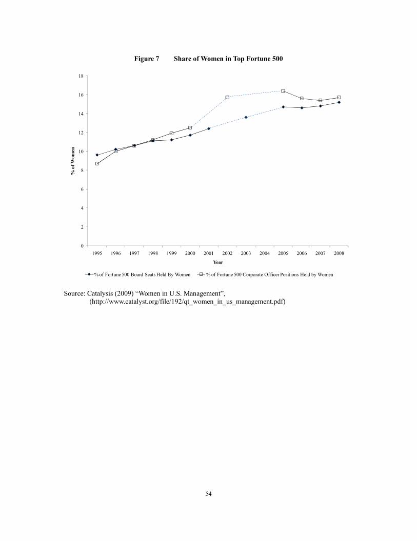
54
Figure 7 Share of Women in Top Fortune 500
0
2
4
6
8
10
12
14
16
18
1995 1996 1997 1998 1999 2000 2001 2002 2003 2004 2005 2006 2007 2008
% of Women
Year
% of Fortune 500 Board Seats Held By Women % of Fortune 500 Corporate Officer Positions Held by Women
Source: Catalysis (2009) “Women in U.S. Management”, (http://www.catalyst.org/file/192/qt_women_in_us_management.pdf)