workforce scheduling with logical constraints: theory … · 2016-01-22 · chapter 1 models from...

Workforce scheduling with logical

constraints:

theory and applications

in call centers

Gabor Dano

This thesis was supervised by

Sandjai Bhulai

and

Ger Koole

Department of Mathematics

Vrije Universiteit

AmsterdamJuly 2004

Contents

Introduction 3

1 Models from the literature 5

1.1 Definitions of terms and sets . . . . . . . . . . . . . . . . . . . . . . . . 51.2 Model of Dantzig . . . . . . . . . . . . . . . . . . . . . . . . . . . . . . . 61.3 Model of Bechtold and Jacobs . . . . . . . . . . . . . . . . . . . . . . . . 71.4 Model of Aykin . . . . . . . . . . . . . . . . . . . . . . . . . . . . . . . . 91.5 Comparison of the models . . . . . . . . . . . . . . . . . . . . . . . . . . 101.6 Model of Thompson . . . . . . . . . . . . . . . . . . . . . . . . . . . . . 13

2 Scheduling model with logical constraints 16

2.1 Decision, indicator variables . . . . . . . . . . . . . . . . . . . . . . . . . 172.2 Logical constraints . . . . . . . . . . . . . . . . . . . . . . . . . . . . . . 202.3 The IP formulation of the logical relationships . . . . . . . . . . . . . . . 222.4 The model with logical constraints . . . . . . . . . . . . . . . . . . . . . 23

2.4.1 Terms, variables and sets . . . . . . . . . . . . . . . . . . . . . . 242.4.2 The constraint set of the model . . . . . . . . . . . . . . . . . . . 252.4.3 The objective function . . . . . . . . . . . . . . . . . . . . . . . . 26

3 Call centers 30

3.1 Introduction . . . . . . . . . . . . . . . . . . . . . . . . . . . . . . . . . . 303.2 Call centers in general . . . . . . . . . . . . . . . . . . . . . . . . . . . . 303.3 Call center characteristics . . . . . . . . . . . . . . . . . . . . . . . . . . 313.4 Mathematics and call centers . . . . . . . . . . . . . . . . . . . . . . . . 313.5 Queueing models in call centers . . . . . . . . . . . . . . . . . . . . . . . 32

3.5.1 The modeling area . . . . . . . . . . . . . . . . . . . . . . . . . . 323.5.2 Queueing models . . . . . . . . . . . . . . . . . . . . . . . . . . . 333.5.3 Little’s Law . . . . . . . . . . . . . . . . . . . . . . . . . . . . . . 353.5.4 PASTA property . . . . . . . . . . . . . . . . . . . . . . . . . . . 363.5.5 The M/M/s queue . . . . . . . . . . . . . . . . . . . . . . . . . . 363.5.6 The M/M/s/N queue . . . . . . . . . . . . . . . . . . . . . . . . 38

3.6 Workforce scheduling in call centers . . . . . . . . . . . . . . . . . . . . 40

Contents 2

4 An application in call centers 42

4.1 The scheduling environment . . . . . . . . . . . . . . . . . . . . . . . . . 424.2 Input parameters . . . . . . . . . . . . . . . . . . . . . . . . . . . . . . . 434.3 The implementation of the model . . . . . . . . . . . . . . . . . . . . . . 45

4.3.1 The objective function in the model . . . . . . . . . . . . . . . . 454.3.2 Logical constraints in the model . . . . . . . . . . . . . . . . . . 45

4.4 Experimental results with the test problem . . . . . . . . . . . . . . . . 46

5 Concluding remarks and future prospects 55

Bibliography 57

Introduction

Nowadays, enterprises and organizations are faced with increasing demand require-ments. On the one hand, it means that they have to provide high quality of servicefor their customers. On the other hand, they would like to satisfy their employees’demand as much as possible. Thus, companies such as airlines, hospitals, police andambulance departments, telephone companies and banks face a very delicate problemwith workforce scheduling.Generally, workforce, labor or personnel scheduling or rostering is the process of design-ing work timetables for employees to satisfy the demand requirements for its services.Different kind of mathematical approaches have developed in order to help the com-panies to solve this problem. According to [6] the development of these mathematicalmodels and algorithms involves the following levels:

1. a demand modeling study that collects and uses historical data to forecast demandfor services and converts these to the staffing levels needed to satisfy servicestandards,

2. consideration of the solution techniques required for a personnel scheduling toolthat satisfies the constraints arising from workplace regulations while best meet-ing a range of objectives including coverage of staff demand, minimum cost andmaximum employee satisfaction,

3. specification of a reporting tool that displays solutions and provides performancereports.

In this master thesis we focus on problems in the second level, i.e., the shift schedulingand the staff assignment problem. The general shift scheduling problem involves de-termining the number of employees to be assigned to each shift to satisfy the demandrequirements. In the staff assignment problem we have the number of required em-ployees for each shift and we have to assign employees for shifts. It is very important,but meanwhile very difficult to find an optimal solution that minimizes the cost andsatisfies employee preferences of these complex and highly constrained problems.

The main interest of this thesis is to introduce and apply a mathematical programmingmodel, which can solve both the shift scheduling and the staff assignment problem. Inthis model we use logical constraints to model different conditions and requirements by

Introduction 4

the government or by the company.

In Chapter 1 we give an introduction of the shift scheduling and the staff assignmentproblems. We discuss different mathematical programming models from the literature,compare them and introduce some basic definitions and terms, which we use afterwardsin the thesis.

In Chapter 2 we build up our labor scheduling model. In the beginning of this chapterwe introduce the way we can use decision variables in a linear programming (LP) orinteger programming (IP) environment to represent connections between certain statesof variables. Later in this chapter we give an introduction of mathematical logic andwe describe how we can model logical relationships in an LP or IP model. Using thesemodeling techniques we build up a labor scheduling model, in which we represent shiftsimplicitly, i.e., we use logical constraints to express them. This model is also describedin this chapter.

In Chapter 3 we give an overview of call centers, in which labor scheduling plays a veryimportant role. Moreover, in this chapter we give a basic introduction on queueingtheory and queueing models, which provide the mathematical background to modeland analyze these centers. We focus on mathematical methods, which we can use toconvert historical data to estimate the number of required agents.

In Chapter 4 we solve a workforce scheduling problem with our model. Afterwards inthis chapter we describe our modeling and implementation method. In the end of thechapter we analyze the experimental results of the test problems.

In Chapter 5 we make some concluding remarks about our modeling method, compu-tational results and we will mention some future prospects.

I would like to thank my supervisors Sandjai Bhulai and Ger Koole for their atten-tion and support during this semester, which enriched my knowledge and experiencein mathematics.

Chapter 1

Models from the literature

In this chapter we would like to introduce the labor scheduling problem. As we alreadymentioned, it has different steps and for each step there are different mathematical pro-gramming models to solve it. In the beginning of this chapter we will deal with threedifferent mathematical programming formulations of the shift scheduling problem. Wewill describe and analyze these models and we will make a comparison between them.After, we will introduce one mathematical programming model for assigning employeesto shifts. All of these models are from the literature.

For dealing with these models it is essential to introduce the following basic definitionsand terms, which we will use afterwards in this thesis.

1.1 Definitions of terms and sets

Definition 1.1.1 A period is a basic interval for which the planning occurs, typically15 min., 30 min. or 60 min.

Definition 1.1.2 A shift is a work schedule for an employee for a specific day, thatsatisfies different restrictions defined by management policy, contractual obligations orgovernmental regulations.

Definition 1.1.3 Work span is the contiguous set of planning periods in which eitherwork or rest must take place for a given shift.

Definition 1.1.4 A tour is a work schedule for an employee for a week, comprisedof separate shifts, that satisfies applicable restrictions defined by management policy,contractual obligations or governmental regulations.

Definition 1.1.5 A service level is a predefined property of the service for measuringits quality.

1.2. Model of Dantzig 6

Definition 1.1.6 A break window is a set of contiguous periods in which the breakoccurs.

Definition 1.1.7 The extraordinary overlap is the existence of the following condition:the initial and final periods in the break window for any one shift type are earlier andlater respectively, than the corresponding initial and final periods in the break windowfor at least one other shift type.

1.2 Model of Dantzig

The shift scheduling problem was introduced first by Edie [5] in 1954. Since his paperthis problem and a number of related ones have attracted considerable attention in theliterature. The first integer programming formulation for the shift scheduling problempresented by Dantzig [4] is the following set-covering type model (DLSM):

min z =∑

t∈T

ctxt, (1.1)

subject to∑

t∈T

atpxt ≥ rp for p ∈ P, (1.2)

xt ∈ N for t ∈ T, (1.3)

where the sets and variables are the following:

P the set of indices associated with planning periods,T the set of indices associated with allowable shifts (tours),

atp

1, if period p is a working period for shift (tour) t,0, otherwise,

ct the cost of having an employee work shift (tour) t,rp the desired staffing level in period p,xt the number of employees working shift (tour) t.

In this DLSM model the objective (1.1) is to minimize the cost of thescheduled shifts (tours), subject to restrictions (1.2) and (1.3).Constraint set (1.2) ensures that sufficient employees are present in all periods.If we give different shift types, lengths, shift start times, number and length of relief(rest), lunch breaks and break windows, the set-covering formulation requires that allpossible combinations of these features are included as different shifts in T .When relief and lunch breaks and break windows are included, the number of shifts inT increases rapidly. Consequently, standard integer programming tools fail to be usefulto solve these extended models because of the extremely high number of shifts in T .

1.3. Model of Bechtold and Jacobs 7

1.3 Model of Bechtold and Jacobs

Bechtold and Jacobs [3] in 1990 applied implicitly matched breaks with explicitly mod-eled shifts. They began to develop this model with the following initial assumptions:

(1) The organization operates less than 24 hours.

(2) All planning periods are of equal length.

(3) Every employee will receive exactly one break.

(4) The duration of the breaks is identical for all shifts that are modeled.

(5) The duration of breaks contains one or more planning periods.

(6) Each shift type is defined by the assignment of a single break window to anassociated work span.

(7) The break window for each shift consists of any selected nonzero subset of periodssubject to the restriction that all periods contained within the break interval mustbe a subset of the work span associated with the shift.

(8) Extraordinary overlap does not exist.

(9) No understaffing is allowed.

With these assumptions, their (BJSSM) model is the following:

min∑

t∈T

ctxt, (1.4)

subject to

∑

Xp −∑

Ωp ≥ rp for p ∈ P, (1.5)∑

Fk −∑

Gk ≥ 0 for all but the last period k ∈ N, (1.6)∑

Rk −∑

Sk ≥ 0 for all but the first period k ∈ M, (1.7)∑

X −∑

B = 0, (1.8)

xt ∈ X, xt ∈ N, (1.9)

bp ∈ B, bp ∈ N, (1.10)

where the sets and the variables of the model are the following:

1.3. Model of Bechtold and Jacobs 8

∑

A the sum of all elements contained in any set A,P the set of indices associated with planning periods,T the set of indices associated with allowable shifts,X xt| t ∈ T ,N the set of final (latest) periods (ascending order)

in the break windows associated with all shifts,M the set of initial (earliest) periods (ascending order)

in the break windows associated with all shifts,Ωp the set of break variables for which period p is a break period,ct the cost of having an employee work shift t,rp the labor requirement in period p,xt the number of employees working shift t,bp the total number of breaks initiated at the start of period p

by the complete set of employees from all shifts,l the earliest period in P in which the break for any shift may begin,u the latest period in P in which the break for any shift may begin,Wt the work span associated with shift t,Xp xt| p ∈ Wt , i.e., the total number of employees working in period p,Vt the set of periods associated with the break window for shift t,Ut bp| p ∈ Vt ,Fk bp| k ∈ N and p = l, l + 1, . . . , k ,Gk xt|Ut ⊆ Fk , i.e., the set of xt where t belongs to those shifts

for which break windows are in the interval ( l, l + 1, . . . , k ) with k ∈ N ,Rk bp| k ∈ M and p = k, k + 1, . . . , u ,Sk xt|Ut ⊆ Rk , i.e., the set of xt where t belongs to those shifts

for which break windows are in the interval ( k, k + 1, . . . , u ) with k ∈ N ,Pb l, l + 1, . . . , u − 1, u ,B bp| p ∈ Pb , i.e., the total number of breaks

initiated in the interval l, l + 1, . . . , u − 1, u .

In this model the objective (1.4) is to minimize the cost of the scheduled shifts, subjectto restrictions (1.5)-(1.10). Constraint set (1.5) ensures that demand requirements aremet in all periods. Constraint sets (1.6) - (1.8) are the control constraints, which areincluded to ensure that the shifts are implicitly represented. Constraint set (1.6) ensuresthat sufficient quantities of breaks are appropriately available for allocation to subsetof shifts with break windows which are fully contained within the successively largerintervals ( l, l + 1, . . . , k ) with k ∈ N . The function of constraint set (1.7) is the sameas constraint set (1.6) except that the successively larger intervals are ( k, k + 1, . . . , u )with k ∈ M . Constraint (1.8) ensures that exactly one break is available for eachemployee scheduled.The proof that the DLSM model is equivalent with this BJSSM is contained in [2] whichwas based upon the initial assumptions. The term equivalence is used to indicate thatthe two models represent the same set of allowed shifts and that the optimal objective

1.4. Model of Aykin 9

function values for the two models are equal.

1.4 Model of Aykin

Aykin’s model [1] is also based on the implicit representation of the break placements.He considered the problem with multiple rest and lunch breaks and multiple breakwindows. He introduced integer variables for the numbers of employees assigned to ashift and starting their breaks in different planning periods within the associated breakwindow. This representation has high flexibility provided by the break windows, i.e.,the number and the length of the break windows are optional in this model.Thus, without loss of generality he assumed that every employee receives two reliefbreaks and one lunch break. Further, it was also assumed that the duration of therelief breaks is one period and the duration of the lunch break is two periods.With these assumptions, Aykin’s general shift scheduling model (ASSM) can be for-mulated as follows:

min∑

t∈T

ctxt, (1.11)

subject to

∑

t∈T

atpxt −∑

t∈T1p

utp −∑

t∈TL(p−1)

wt(p−1) −

−∑

t∈TLp

wtp −∑

t∈T2p

vtp ≥ bp for p ∈ P, (1.12)

xt −∑

p∈B1t

utp = 0 for t ∈ T, (1.13)

xt −∑

p∈BLt

wtp = 0 for t ∈ T, (1.14)

xt −∑

p∈B2t

vtp = 0 for t ∈ T, (1.15)

xt, utp, wtp, vtp ∈ N, (1.16)

where the sets and the variables in the model are the following:

xt the number of employees working shift t,bp the number of employees needed in period p,

atp

1, if period p is a working period for shift (tour) t,0, otherwise,

utp the number of employees assigned to shift tand starting their first relief break in period p,

1.5. Comparison of the models 10

wtp the number of employees assigned to shift tand starting their lunch break in period p,

vtp the number of employees assigned to shift tand starting their second relief break in period p,

T the set of indices associated with allowable shifts,P the set of indices associated with periods,B1t the set of planning periods in which an employee working shift t

may start his/her first relief break,B2t the set of planning periods in which an employee working shift t

may start his/her second relief break,BLt the set of planning periods in which an employee working shift t

may start his/her lunch break,T1p the set of shifts for which period p is a break start time

within the time windows for the first relief break,T2p the set of shifts for which period p is a break start time

within the time windows for the second relief break,TLp the set of shifts for which period p is a break start time

within the time windows for the lunch break.

In this scheduling model the objective (1.11) is to minimize the cost of the scheduledshifts subject to the constraint sets (1.12)-(1.16). With constraint set (1.12) we ensurethat sufficient number of employees are present in all periods. Every employee has totake exactly one first, one second relief break and one lunch break. We model theseconditions with constraint sets (1.13)-(1.15), where constraint set (1.13) is responsiblefor the first relief breaks, constraint set (1.14) is responsible for the lunch breaks andconstraint set (1.15) is responsible for the second relief breaks.

This model can be extended with additional restrictions on break placements and shifttypes.For example, Aykin suggested the following constraint to model the situation when thenumber of employees taking a break in a period p has to be limited because of spaceavailability or company policy.

∑

t∈T1p

utp +∑

t∈TL(p−1)

wt(p−1) +∑

t∈TLp

wtp +∑

t∈T2p

vtp ≤ hp. (1.17)

It is possible to model shifts with different lengths or number of breaks with thisformulation by introducing a new set of break variables and new break constraints forevery additional break.

1.5 Comparison of the models

In the previous sections we introduced three different formulations of the shift schedul-ing problem: Dantzig [4], Bechtold and Jacobs [3] and Aykin [1].


In this section we compare these models, focusing on the number of variables and thenumber of constraints in them.

First, we will introduce notations for the cardinality of the following sets:

|P | = nP , where P is the set of indices associated with planning periods,

|T | = nT , where T is the set of indices associated with allowable shifts,

|N | = nN , where N is the set of final (latest) periods (ascending order)in the break windows associated with all shifts,

|M | = nM , where M is the set of initial (earliest) periods (ascending order)in the break windows associated with all shifts,

|Vt| = nVt, where Vt is the set of periods associatedwith the break window for shift t,

|B| = nB, where B = bp| p is in the set of break periods and bp

is the total number of breaks initiated at the start of period p,

|B1t| = n1t, where B1t is the set of planning periods in which an employeeworking shift t may start his/her first relief break,

|BLt| = nLt, where BLt is the set of planning periods in which an employeeworking shift t may start his/her lunch break,

|B2t| = n2t, where B2t is the set of planning periods in which an employeeworking shift t may start his/her second relief break.

Let us denote with NC(P ) the number of constraints in any mathematical program-ming model P and with NV (P ) the number of variables in that model.In our analysis, we deal with the DLSM, the BJSSM and the ASSM scheduling modelsand analyze them from this point of view .

With the introduced notations, we have the following results:

NC(DLSM) = nP , (1.18)

NV (DLSM) =∑

t∈T

nVt =∑

t∈T

n1tnLtn2t, (1.19)

NC(BJSSM) = nP + nM + nN − 1, (1.20)

NV (BJSSM) = nT + nB, (1.21)

NC(ASSM) = 3nT + nP , (1.22)

NV (ASSM) = nT +∑

t∈T

(

n1t + nLt + n2t

)

. (1.23)

Equation (1.18) comes directly from the constraint set (1.2) in the model of Dantzig onpage 6. In that model we formulate all shifts implicitly; thus on one hand, if we have


Vt break periods for any t ∈ T then we have altogether∑

t nVt variables in it. On theother hand, if we have n1t, n2t, nLt number of periods for the first, the second reliefbreak and the lunch break respectively for any t ∈ T , we should multiply them andsum the result over all shifts t. This result is shown in equation (1.19).

In the model of Bechtold and Jacobs on page 7, we have the constraint set (1.6) for allperiods in N except the latest period and the constraint set (1.7) for all periods in Mexcept the earliest one. This implies that we have nN − 1 + nM − 1 constraints fromthese sets, nP from the constraints in equation (1.5) and an additional one from equa-tion (1.6). Hence, we get the result in (1.20). Result (1.21) is derived from constraints(1.9) and (1.10) on page 7.

In Aykin’s model on page 9, we assumed that there are three breaks for every employee.This assumption has a big effect on the number of constraints and variables in formulas(1.22) and (1.23). The previous result comes from constraint set (1.12), where we havenP constraints and from equation (1.12)-(1.14), where we have nT constraints for eachbreak. In this model we have one variable for each shift t and n1t, n2t and nLt for anyperiod t. These results lead us to equation (1.23).

We can easily make a comparison between the DLSM and the BJSSM model. Fromresult (1.18) and (1.20) is it clear that in the model of Dantzig we have less constraints.If we would like to compare the number of variables in these two models, we have to doa more in-depth analysis. If break flexibility is not modeled, then NV (BJSSM) = nT ,so we have less variables in the DLSM model. However, the relative advantage in usingthe BJSSM formulation increases significantly when nVt is increasing, because in thiscase the number of variables increases rapidly in the Dantzig model.

In the comparison between Dantzig’s model and the model of Aykin we can see thatthere are less constraints than in the previous model, i.e., if we compare equation (1.18)and (1.22). As for the variables, in the Dantzig model we have a product of three vari-ables (or even more if we have more breaks) and in the Aykin model we have the sumof them. From this we can conclude that if n1t, n2t and nLt are big enough then Aykin’smodel has less variables.

If we would like to compare the BJSSM and the ASSM model we have a little prob-lem, because these models model different scheduling problems. The main differencebetween them is the number and the length of breaks: we have three breaks in Aykin’smodel (one is two periods) and one break in Bechtold and Jacobs model. To be ableto compare them we have to model the similar problem with these formulations.Fortunately, it is possible to model a scheduling problem with one break, which is oneperiod long, with both models. In this case results of the BJSSM model remain true,

1.6. Model of Thompson 13

i.e., equation (1.20) and (1.21), but we have to modify Aykin’s model in the followingway: we have to use only the variables and the constraints, which are for the first reliefbreak. In this case we have nP constraints from constraint set (1.12) and nT fromconstraint set (1.12), which means that we have nP + nT constraints in this model,i.e., in this case NC(ASSM) = nP + nT . This result is comparable with the result inequation (1.20). Using the same logic as above we have that in Aykin’s model thereare nT +

∑

t∈T n1t variables, which is comparable also with the number of variables inthe BJSSM model in equation (1.21).

So far in this chapter we introduced and analyzed three different mathematical pro-gramming approaches for the shift scheduling problem. In the next section we willintroduce a model for assigning employees to shifts.

1.6 Model of Thompson

In this section we deal with Thompson’s model [8] for assigning employees to shifts withsome special characteristics. There are some initial restrictions in the model, which arethe following:

(1) All shifts have to be assigned. These shifts were identified by the schedulerpreviously.

(2) It is obliged contractually to satisfy preferences for shifts in order of employeeseniority, i.e., a senior employee receives his/her desired maximum number ofshifts before a less senior employee receives more than one shift.

(3) Employees have special characteristics:

(a) availability, i.e., the time when they are available and the maximum numberof shifts they can work,

(b) skills and location,

(c) all employees receive at least one shift per week,

(d) an employee cannot be assigned more than one shift per day.

With these restrictions, Thompson’s model is the following:

minP0

∑

t∈T

ut +∑

e∈E

Pe

(

∑

t∈T |ct ∈Ce,dt ∈De

vetxet

)

(1.24)

subject to


∑

e∈E|ct ∈Ce,dt ∈De

xet + ut = 1 for t ∈ T, (1.25)

∑


xet ≥ 1 for e ∈ E, (1.26)

∑


xet ≤ me for e ∈ E, (1.27)

∑

t∈T |ct ∈Ce,dt=i

xet ≤ 1 for e ∈ E, i ∈ De, (1.28)

∑


xet ≤ 1 + (me − 1)ye−1 for e ∈ E|e > 1 , (1.29)

∑


xet ≥ meye for e ∈ E|e < E , (1.30)

xet ∈ 0, 1 for e ∈ E, t ∈ T |ct ∈ Ce, dt ∈ De , (1.31)

ye ∈ 0, 1 for e ∈ E|e < E , (1.32)

ut ∈ 0, 1 for t ∈ T, (1.33)

where the sets and the variables of the model are the following:

T the set of shifts,E the set of employees, ordered from most senior to least senior,Pi the priority of component i, where Pi Pi+1

(the priority for component i is much larger thanthe priority for component i + 1),

Ce the set of shift categories that employee e can work,De the set of days that employee e can work,

xet

1, if employee e is assigned to shift s,0, otherwise,

me the maximum number of shifts to assign to employee e,vet the undesirability of assigning employee e to shift t,

ye

1, if employee e is assigned the maximum number of shifts,0, otherwise,

ct the category of shift t,dt the day on which shift t is scheduled,

ut

1, if shift t is unassigned,0, otherwise.

In this model the objective (1.24) is to minimize the number of unassigned shifts andspecify that employees’ shift choices are to be satisfied, if possible, in order of seniority.


With constraint set (1.25) we ensure that all shift will be assigned, i.e., minimizing thenumber of unassigned shifts ut. We have to assign at least one shift to each employee.We model this condition with constraint set (1.26). Constraint set (1.27) ensures thatwe assign no more than the maximum desired number of shifts for each employee andconstraint set (1.28) ensures that no more than one shift per day per employee is as-signed. With constraint set (1.29)-(1.31) we force a more senior employee to work theirdesired number of shifts before a less senior employee works more than one shift.

In the next chapter we will introduce our workforce scheduling model. In this modelwe will present and use a different approach for formulating labor scheduling problems.

Chapter 2

Scheduling model with logical

constraints

In the previous chapter we introduced three mathematical programming models of theshift scheduling problem and one mathematical programming model for the employeeassignment problem. In these shift scheduling models we saw different techniques formodeling the breaks: explicit modeled breaks in Dantzig model [4], implicit modeledbreaks in Bechtold and Jacobs’s [3] and Aykin’s model [1]. In all of these models theshifts are represented by the set T , which means that in these models the allowableshifts are explicitly in the model. In Thompson’s model [8] we saw a modeling tech-nique, with which we can assign shifts to employees and satisfy employees’ preferencesfor shifts in order of seniority.

In this chapter we will introduce our labor scheduling model, in which we will modelshifts implicitly. For this reason at the beginning of the chapter we will deal with therelationship between mathematical logic and operation research, i.e., the way we canrepresent logical constraints with LP or IP formulation. Using this formulation we canprovide high flexibility with involve different rules to the model, with which we canmodel shifts in an implicit way. In our model we will distinguish between employeeswith a long term contract and employees, who can work only in specific periods a day(e.g., students, part time workers, etc.). It is possible that we have employees, whohave long term contract, with different skills, experiences and different preferences, i.e.,we have different employees for different types of work and they would like to work indifferent periods (e.g., an employee does not want to work in the night or he/she wouldlike to finish his/her work earlier). We will model these preferences in the followingway: we will penalize if an employee has to work in the period, in which he/she doesnot want and vice versa.

At the end of the chapter we will present our shift scheduling model, which we will useto solve a scheduling problem from call centers in Chapter 4.

2.1. Decision, indicator variables 17

2.1 Decision, indicator variables

In a linear programming (LP) or integer programming (IP) environment we may useadditional variables to represent connections between different variables and states.In this section we will introduce the connection between certain states of a continuousvariable and states of its indicator or decision variable. In our representation the in-dicator and decision variables are always 0-1 variables. We will denote the LP or IPvariables with x or xi and the indicator or decision variable with δ.

It is a frequently occuring situation when we want to distinguish between the statewhere x = 0 and the state when x > 0. For this we can use an indicator variable δ. Byintroducing the following constraint we can force δ to take value 1 when x > 0:

x − Mδ ≤ 0, (2.1)

where M is a constant coefficient representing a known upper bound for x.With inequality (2.1) we now have logically the following condition:

x > 0 → δ = 1. (2.2)

Now we would like to impose the other condition, that is

x = 0 → δ = 0, (2.3)

or equivalently,δ = 1 → x > 0. (2.4)

Together condition (2.2) and condition (2.3) or (2.4) impose the following logical rela-tion:

δ = 1 ↔ x > 0. (2.5)

It is not possible to represent (2.4) by a constraint. Instead we can find a realisticlower bound m for the continuous variable x. With this lower bound we can satisfy thecondition:

δ = 1 → x ≥ m. (2.6)

For this we can use the following constraint:

x − mδ ≥ 0. (2.7)

In the above described method we only use the decision variable δ to distinguish betweentwo states of one continuous variable. It is possible to use indicator variables in a similarway to show whether an inequality holds or does not hold.

First, we wish to indicate whether the following inequality holds by means of an indi-cator variable δ:

∑

j

ajxj ≤ b.


Therefore we would like to model the following condition first:

δ = 1 →∑

j

ajxj ≤ b. (2.8)

Condition (2.8) can be represented by a constraint:

∑

j

ajxj + Mδ ≤ M + b. (2.9)

The usual way of constructing (2.9) from condition (2.8) is the following method.

First, we would like to establish the logical condition, δ = 1 →∑

j ajxj ≤ b,that is equivalent with the condition:δ = 1 →

∑

j ajxj − b ≤ 0.In the other way it means, that if (1 − δ) = 0 then we wish to have

∑

j ajxj − b ≤ 0.This condition is imposed if

∑

j

ajxj − b ≤ M(1 − δ),

where M is a sufficiently large upper bound, such that it does not give an undesiredconstraint.Now the next step is to model the reverse implication of constraint (2.8), i.e.,

∑

j

ajxj ≤ b → δ = 1. (2.10)

This can be expressed with the following condition, which is equivalent with (2.10):

δ = 0 →∑

j

ajxj 6≤ b, (2.11)

i.e.,

δ = 0 →∑

j

ajxj > b. (2.12)

When we are dealing with the expression∑

j ajxj > b, we run into the same difficultiesthat we met with the expression x > 0 in condition (2.4).We must rewrite the expression

∑

j

ajxj > b,

as∑

j

ajxj ≥ b + ε,


where ε is some small tolerance value beyond which we will regard the constraint ashaving been broken.If the coefficients aj are integers as well as the variables xj for all j, there is no difficultyas ε can be taken equal to 1.With this ε (2.12) may now be written as:

δ = 0 →∑

j

ajxj − (b + ε) ≥ 0. (2.13)

Now we can represent condition (2.13) with a constraint, which is:

∑

j

ajxj − (m − ε)δ ≥ b + ε, (2.14)

where m is a lower bound for expression∑

j ajxj − b.

Using the above described method for inequalities, which are of the form∑

j ajxj ≤ b ,we can indicate whether an inequality of the form

∑

j

ajxj ≥ b

holds or not.We only have to transform the relation ‘≥’ into the relation ‘≤’.The logical condition

δ = 1 →∑

j

ajxj ≥ b (2.15)

can be represented with the inequality

∑

j

ajxj + mδ ≥ m + b, (2.16)

where m is again the lower bound of the expression

∑

j

ajxj − b.

For the conditionδ = 0 →

∑

j

ajxj < b (2.17)

when applying the described method, we get the following constraint,

∑

j

ajxj − (M + ε)δ ≤ b − ε, (2.18)

2.2. Logical constraints 20

where M is again the upper bound for the expression∑

j ajxj − b.

Finally, to use an indicator variable δ for a constraint of the form ‘=’ such as

∑

j

ajxj = b,

is more complicated.We can use δ = 1 to indicate that the ‘≤’ and ‘≥’ cases hold simultaneously. This isdone by stating both (2.9) and (2.16) together.If δ = 0 we want to force either the ‘≤’ or the ‘≥’ constraint to be broken.This can be done by expressing (2.14) and (2.18) with two variables δ1 and δ2 giving

∑

j

ajxj − (m − ε)δ1 ≥ b + ε, (2.19)

∑

j

ajxj − (M + ε)δ2 ≤ b − ε. (2.20)

The indicator variable δ forces the required condition by the extra constraint

δ1 + δ2 − δ ≤ 1. (2.21)

2.2 Logical constraints

In the previous section it was pointed out that extra 0-1 variables can be introducedinto an LP or IP model as decision variables or indicator variables. In these models ithas frequently happened that we have to model also the logical connections betweenthese decision or indicator variables with linear programming tools. Including theseconnections in a mathematical programming model we will able to represent real lifeproblems in a more efficient way.In this section we will introduce some basic concepts and properties from mathematicallogic, which are necessary from the modeling point of view.

It will be convenient to use notations from Boolean algebra. First of all we would liketo introduce the so called set of connectives. In general, connectives are often used tomake compound propositions. The main ones are shown in the following table (p andq are given propositions):

2.2. Logical constraints 21

Name Symbol Representation Meaning

negation ¬ ¬p ‘not p’conjuction ∧ p ∧ q ‘ p and q’disjunction ∨ p ∨ q ‘p or q (or both)’implication → p → q ‘if p then q’biconditional ↔ p ↔ q ‘p if and only if q’

Table 2.1: Main compound propositions

The truth value of these compound propositions only depends on the truth value ofits components. It is quite important to understand how the propositions value willchange if the value of a component changes. These relations are shown in Table 2.2,where p, q, are given propositions, t is written if a statement is true and f if it is false.

p q ¬p p ∧ q p ∨ q p → q p ↔ q

t t f t t t tt f f f t f ff t t f t t ff f t f f t t

Table 2.2: Truth table of main compound propositions

There are some equivalences (≡) between these propositions, that are sufficient fordealing with connectives. In the following, we will explore these equivalences.Let p, q and r be given propositions, t stands for true and f stands for false statements.With these terms, we have the following laws:

Idempotent laws

p ∨ p ≡ p , p ∧ p ≡ p . (2.22)

Commutative laws

p ∨ q ≡ q ∨ p , p ∧ q ≡ q ∧ p . (2.23)

Associative laws

(p ∨ q) ∨ r ≡ p ∨ (q ∨ r) , (p ∧ q) ∧ r ≡ p ∧ (q ∧ r) . (2.24)

2.3. The IP formulation of the logical relationships 22

Distributive laws

p ∨ (q ∧ r) ≡ (p ∨ q) ∧ (p ∨ r) , (2.25)

p ∧ (q ∨ r) ≡ (p ∧ q) ∨ (p ∧ r) . (2.26)

Domination laws

p ∨ t ≡ t , p ∧ t ≡ p , p ∨ f ≡ p , p ∧ f ≡ f , (2.27)

p ∨ ¬p ≡ t, p ∧ ¬p ≡ f , ¬t ≡ f , ¬f ≡ t . (2.28)

Double negation law

¬¬p ≡ p . (2.29)

De Morgan’s laws

¬(p ∨ q) ≡ ¬p ∧ ¬q , ¬(p ∧ q) ≡ ¬p ∨ ¬q . (2.30)

Implication lawsp → q ≡ ¬p ∨ q . (2.31)

¬(p → q) ≡ ¬(¬p ∨ q) ≡ p ∧ ¬q , (2.32)

¬q → ¬p ≡ ¬¬q ∨ ¬p ≡ p → q , (2.33)

p → (q ∧ r) ≡ (p → q) ∧ (p → r) , (2.34)

p → (q ∨ r) ≡ (p → q) ∨ (p → r) , (2.35)

(p ∧ q) → r ≡ (p → r) ∨ (q → r) , (2.36)

(p ∨ q) → r ≡ (p → r) ∧ (q → r) . (2.37)

2.3 The IP formulation of the logical relationships

In the previous sections we introduced indicator, decision variables to distinguish be-tween certain states of the variables in an LP or IP model. Afterwards we dealt withsome basic concepts from mathematical logic to give a background for manipulatingwith these variables.In this section we would like to describe how we can model these Boolean algebraicmanipulations with equalities and inequalities in an LP or IP modeling area.From now on we will use Xi to stand for a proposition with truth value δi ∈ 0, 1 i.e.,Xi is true if and only if δi = 1, where δi ∈ 0, 1.The following propositions and constraints are equivalent [9]:

X1 ∨ X2 ≡ δ1 + δ2 ≥ 1, (2.38)

X1 ∧ X2 ≡ δ1δ2 = 1 ≡ δ1 = 1, δ2 = 1, (2.39)

2.4. The model with logical constraints 23

¬X1 ≡ δ1 = 0, (2.40)

X1 → X2 ≡ δ1 − δ2 ≤ 0, (2.41)

X1 ↔ X2 ≡ δ1 − δ2 = 0. (2.42)

If a product term such as δ1δ2 were to appear anywhere in a model, the model couldbe made linear by the following steps:

(i) replace δ1δ2 by a 0 − 1 variable δ3,

(ii) impose the logical condition

δ3 = 1 ↔ δ1 = 1, δ2 = 1 (2.43)

by means of the extra constraints

−δ1 + δ3 ≤ 0,

−δ2 + δ3 ≤ 0, (2.44)

δ1 + δ2 − δ3 ≤ 1.

It is even possible to linearize terms involving a product of a 0-1 variable δ with acontinuous variable x. The term xδ can be treated in the following way:

(i) replace xδ by a continuous variable y ,

(ii) impose the logical conditionδ = 0 → y = 0,

δ = 1 → y = x.

by the extra constraintsy − Mδ ≤ 0,

−x + y ≤ 0, (2.45)

x − y + Mδ ≤ M,

where M is an upper bound for x (and hence also y).

2.4 The model with logical constraints

So far in this chapter we established the mathematical background for representinglogical relationships between variables in mathematical LP or IP programming. Withthis we will create a model in which these relations are involved.In this section we will focus on the workforce scheduling problems. In our model wewill use logical constraints to represent different restrictions (e.g., management policy,contractual obligations, governmental regulations, etc. ). To deal with the model it issufficient to introduce some new terms and definitions (the definitions from Section 1.1will be used also here).


2.4.1 Terms, variables and sets

In the constraint set of the model we will use the following variables and sets:

I the index set of employees,K the index set of different types employees,Tk the index set of employees from type k, where k ∈ K,P the index set of periods,

n(k)p the number of employees needed in period p from type k,

xpi

1, if employee i is hired for period p,0, if employee i is not hired for period p,

y(k)pe the number of extra employees for period p from type k.

Logic(X) all the necessary logical constraints on matrix X,of which the elements are denoted by xpi.

With index set K we can represent different types of employees, e.g., if there are dif-ferent skills for handling different types of jobs. This situation occurs frequently forexample in call centers (we will discuss this topic in Section 3.3). We use the index setTk to group employees according to their skills. Set P was already defined and used inthe previous models from literature in Chapter 1.Because we have different types of employees, who can handle different jobs, we needto distinguish between required levels of staffing for all types. We will use parameter

n(k)p in our model to make this distinction between the required number of workers in

all types. The variable xpi ∈ 0, 1 is for scheduling employees into periods.

We already made a distinction between employees with different skills. It is quiterational to differentiate employees who have a long term contract with the companyand employees who are applying for a part time job with exact requirements for theirworking time, i.e., they have periods in which they can work and periods in which itis impossible for them to work. For this reason we will introduce index set Ic for theemployees with a long term contract and index set Ip for employees with a part timejob.Notice that,

Ic ∩ Ip = ∅

and

Ic ∪ Ip = I.


It is possible that we do not have enough employees to satisfy the required level (e.g.,we do not have enough employees in set Ic and there are only a few members in Ip).The companies usually try to avoid this situation but in case of unpredictably highload they have to hire extra workers (e.g., those who have a day off). In our model

we denote with y(k)pe the number of extra employees for period p from type k. These

employees are far the most expensive ones so we will try to avoid to use them.

In our model we will use matrix A to represent the exact possible working times foremployees with a part time job (i.e., employees in the index set Ip):

api

1, if employee i can work in period p,0, if for employee i period p is not a possible working period.

2.4.2 The constraint set of the model

With the terms and notations from the previous section the constraint set of ourscheduling model is the following:

A − X1 ≥ 0∑

i∈Tk

xpi + y(k)pe ≥ n(k)

p ∀k, p

Logic(X)

PLC .

Because we give indexes to employees it is possible to partition X into to submatrices,i.e., X = [X1 X2]. In this partition X1 is a sub-matrix of X, of which the columns are

representing employees with a part time job, i.e., X1 ∈ 0, 1|P|×|Ip| and sub-matrix

X2 ∈ 0, 1|P|×|Ic| is representing employees with a long term contract.In our model we use constraint

A − X1 ≥ 0

to schedule only those part time employees to a period, who are able to work in thatone. It is very important that this constraint has only effect on employees with a parttime job (employees in index set Ip), because we formulate their exact requirementsfor working time with it.With the second constraint, i.e.,

∑

i∈Tk


p ∀k, p

we ensure that sufficient number of employees are present for every period from every

type. This constraint is always satisfiable because of y(k)pe and thus our PLC is always

feasible.In the Logic(X) part it will be useful if we put rarely or never changing constraints (e.g.,governmental restrictions, special characteristics of the firm, contractual obligations,etc.).


2.4.3 The objective function

In the previous section we defined and introduced the constraints for our model. As inevery mathematical programming model, we should define an objective function, withwhich we can express the goals of the model. This part of the modeling method is quitecomplicated because we should find the proper balance between our goals.In this section we will focus on our objectives and the way we can involve them intothe model.

Afterwards we will use SPLCto denote the solution set of PLC , i.e.,

SPLC=

(X, y) ∈ 0, 1|P|×|I| × N|P|·|K|

∣

∣

∣

∣

∣

∣

∣

∣

∣

A − X1 ≥ 0∑

i∈Tk


p ∀k, p

Logic(X)

. (2.46)

We would like to introduce a binary relation between the X2 partitions of X in SPLCto

represent the preferences of employees with a long term contract (e.g., employees canprefer a schedule for themselves against another one).We will use the following notation for this partition set:

ScPLC

:=

Y

∣

∣

∣

∣

X =[

X1 Y]

, X ∈ SPLC

.

There are some basic and rational properties of a preference relation , that we wouldlike satisfy. These are the following:

Definition 2.4.1 If is a binary relation in S cPLC

, then we can define two other binaryrelations with

Z ≺ V ⇐⇒ Z V and V Z

and

Z ∼ V ⇐⇒ Z V and V Z,

∀ Z, V ∈ ScPLC

.

A binary relation is transitive, if

Z V and V W =⇒ Z W,

∀ Z, V, W ∈ ScPLC

.

A binary relation is complete, if

Z V or V Z,

∀ Z, V ∈ ScPLC

.


These properties are very natural if we want to model the preference of employees.With a preference relation we can distinguish between ‘good’ and ‘bad’ objects (sched-ules). This distinction is based on the subjective order of the decision maker. We canrepresent this order with a metric, which expresses the distance between an optimalschedule and any other schedules in S c

PLC.

We will denote with S∗ the optimal schedule for employees with a long term contracts(i.e., all employees having their ideal schedule for the day). In this S∗ ∈ 0, 1|P|×|Ic|

the columns represent the employees, the rows represent the periods (as in X). So

S∗pi

1, if employee i would like to work in period p,0, if employee i would not like to work in period p.

With this ideal schedule we can measure the quality of any other schedules. The rea-sonable way to do this is to consider a schedule ‘good’ if it is ‘near’ to the ideal one andconsider a schedule ‘bad’ if it is ‘far’ from the ideal one. It is important to see that S ∗

is not necessary an element of the set S cPLC

.To deal with such notations as ‘near’ and ‘far’ we will introduce a metric between ma-trices in 0, 1|P|×|Ic| space.

Definition 2.4.2 A metric space M = (X , d) consists of a set X together with afunction, called metric, d : X × X −→ R such that

i) d(x, y) ≥ 0 for all x, y ∈ X , and d(x, y) = 0 ⇐⇒ x = y,

ii) d(x, y) = d(y, x) for all x, y ∈ X ,

iii) d(x, z) ≤ d(x, y) + d(y, z) for all x, y, z ∈ X .

As we can see, the definition of metric space allows us to define different kinds ofmetrics. For our purposes, we will use the so called discrete metric. This is defined by

d0(x, y) =

0, if x = y,1, if x 6= y.

Using this metric, we can define a metric in our 0, 1|P|×|Ic| space, such that

dM (X,Y ) =∑

p,i

vid0(Xpi, Ypi),

where

vi positive integer weight for column i(in our model we will represent the value or the seniority of the employee with it).


Lemma 2.4.1 The space M = (0, 1|P|×|Ic| , dM ) is a metric space, with

dM : 0, 1|P|×|Ic| × 0, 1|P|×|Ic| −→ N.

Proof of Lemma 2.4.1

To proof that dM is a metric we should show that it satisfies all the properties inDefinition 2.4.2.First, we would like to prove property i) from the definition:

dM (X,Y ) =∑

p,i

vid0(Xpi, Ypi)

and

vid0(Xpi, Ypi) ≥ 0 ∀ p, i

thus, dM (X,Y ) ≥ 0. The function dM (X,Y ) = 0 if and only if vid0(Xpi, Ypi) = 0 forall p, i, thus

dM (X,Y ) = 0 if and only if X = Y,

which means that dM (X,Y ) satisfies property i).

Now we would like to prove property ii), i.e., the symmetry:

dM (X,Y ) =∑

p,i

vid0(Xpi, Ypi) =∑

p,i

vid0(Ypi, Xpi) = dM (Y,X),

which means that dM (X,Y ) satisfies property ii).

Finally, we show that dM satisfies property iii), i.e., it satisfies the triangle inequality:

dM (X,Z) =∑

p,i

vid0(Xpi, Zpi) ≤∑

p,i

vi

(

d0(Xpi, Ypi) + d0(Ypi, Zpi))

=

=∑

p,i

vid0(Xpi, Ypi) +∑

p,i

vid0(Ypi, Zpi) = dM (X,Y ) + dM (Y,Z),

which means that dM (X,Y ) satisfies property iii).As we can see our dM function satisfied all the sufficient properties, thus dM (X,Y ) isa metric. It is also clear that dM (X,Y ) satisfy the natural conditions in Definition 2.4.1.

So far we introduced a metric, with which we can represent the preferences of employ-ees. Using this metric, one of our goal is to minimize the distance between the optimalschedule S∗ and the solution, which means that we would like to give the ‘best’ possibleschedule.

We have another very natural goal in our model. It is to minimize the cost of theschedule, i.e., minimize the cost of employees. For this we would like to introduce thefollowing notations:


c(k)pe the cost of extra employees for period p from type k,

cpi the cost of employee i for period p, i ∈ I.

With these notations our objective function is the following:

minw1

[

∑

p∈Pk∈K

c(k)pe y(k)

pe +∑

i∈Ip∈P

cpixpi

]

+ w2dM (S∗, X2). (2.47)

In this objective function w1 and w2 are weights to determine the balance between thecost part and the preference part.

Finally, we have all elements to introduce our labor scheduling model, which is

minw1

[

∑

p∈Pk∈K

c(k)pe y(k)

pe +∑

i∈Ip∈P

cpixpi

]

+ w2dM (S∗, X2), (2.48)

subject toA − X1 ≥ 0∑

i∈Tk


p ∀k, p

Logic(X)

PLC . (2.49)

Chapter 3

Call centers

Up to this point we dealt with the basic staff scheduling models and we set up a modelwith logical constraints.In this chapter we study the world of call centers; a real life area, where workforcescheduling plays a very important role.First we will give a basic introduction about these centers.After we will discuss some basic concepts from queueing theory; a field of mathematics,which helps us to model call centers.Finally, we will go into details of workforce scheduling in call centers, to introduce thisfield of problems for the next chapter where we will solve a specific workforce schedulingproblem.

3.1 Introduction

Nowadays, the most preferred and frequently used way for companies to communicatewith their customers are call centers and their contemporary successors, contact cen-ters. The economic role of these centers is thus significant and rapidly expanding.Most organizations with customer contact - private companies, as well as governmentand emergency services - have re-engineered their infrastructure to communicate withcustomers via call centers.For many companies operating world-wide, such as airlines, banks, credit card compa-nies call centers provide a primary link between customer and service provider.

3.2 Call centers in general

From Koole [7]: “A call center can be considered as a set of resources - typically per-sonnel, telecommunication equipment and computers - which enable to deliver differentkind of services via the telephone”.More generally, a current trend is the extension of the call center into a contact center,which is a call center in which the traditional telephone service is enhanced by some

3.3. Call center characteristics 31

additional multi-media customer-contact channels, commonly e-mail, fax, Internet orchat.

3.3 Call center characteristics

Call centers can be categorized along many dimensions. Call centers with differentcharacteristics can have huge differences from the mathematical point of view. Thus itis very important to determine the basic characteristics of our center before we startto build a mathematical model of it. The functions that call centers can provide varyhighly: help desk for computer software, emergency response (e.g., police, ambulanceetc.), costumer service, tele-marketing and order taking.They greatly vary in size and geographic dispersion, from single-located centers withfew agents that take local calls to large multi-site international centers in which thou-sands of agents work at any time.

Modern call centers are challenged with multitude types of calls, coming in over differ-ent communication channels (telephone, Internet, fax, e-mail, chat mobile devices, . . .), thus these centers require agents with the skill to handle one or more types of calls(single- vs. multi-skilled agents). When multiple skills are required to handle calls, acenter may cross-train low-skilled employees to handle all type of calls.Due to the growing complexity of contact centers the organization of work becomesmore complex. A recent trend in networking is skill based routing that is used to routecalls to appropriate agents.

The central characteristic of a call center is whether it handles inbound or outboundcalls. Inbound call centers handle incoming calls that are initiated by outside callerscalling to a center. Typically, these types of centers provide costumer support, helpdesk services, reservation and sales support for airlines and hotels, and order-takingfunctions for catalog and web-based merchants.Outbound call centers handle outgoing calls, calls that are initiated from within a cen-ter. These types of operations have been traditionally associated with advertisement,tele-marketing and survey businesses. A recent development in some inbound centersis to initiate outbound calls too.

3.4 Mathematics and call centers

In every call center the typical goal is to provide service at a given quality, subjectto a given budget. Call center managers are thus faced with the problem of havinga high service level with rapidly changing inbound calls. This service level is usuallyquantified in terms of congestion or other performance measures.

Because of this highly variable environment, the performance in terms of the qual-

3.5. Queueing models in call centers 32

ity of the service is always changing. For providing an acceptable service level duringoperation hours we have two possibilities.The first possibility is to monitoring the performance and if it reaches an unacceptablelevel; for example, too many customers waiting or too many agents are idle, then react.The second possibility is to build up a mathematical model for supporting the designor the control of the center.In the first case the reaction is based on subjective experiences and in this case thiscould lead to a bad decision if the resulting performance is worse than expected. Usingmathematical models, which are usually based on analytical approaches from Oper-ations Research and Queueing Theory, we can control the performance between ac-ceptable levels. These models have become integral parts of the widely used workforcescheduling tools.

3.5 Queueing models in call centers

In the previous section we discussed the importance of using mathematical models incall centers. In this section we deal with these queueing models.

3.5.1 The modeling area

In the service area, where customers and service providers establish contact, we canoften face queues and queueing problems. Call centers thus can be viewed, naturallyand usefully as queueing systems. This is clear from Figure 3.1 which is a simple callcenter operational scheme.In this queueing system we have the following elements:

arrivals - group of customers those whose are calling the center

queue - a queue of customers those whose are waiting for the service

agents - call center employees who respond to calls

busy signals - if all lines are busy and there is no space in the queue of callers

abandonment - if the customer does not want to wait in the queue anymore

retrials - if a customer tries to contact the center immediately after he/she had a busyline or an abandonment

lost calls - if a customer leaves the call center without being served and he/she doesnot contact immediately after it.

Although this is an operational scheme of a call center, modern call (contact) cen-ters have more complex characteristics as we already discussed it in Section 3.3. Thesecenters are thus more complicated queueing networks and modeling them is a difficult


problem full of challenges.

Figure 3.1: Call center operational scheme

3.5.2 Queueing models

In this subsection we would like to lay down the basic mathematical background ofqueueing theory. The basic queueing model is shown in Figure 3.2.

Figure 3.2: Basic queueing system

There is a wide variety of different queueing models, but there are some basic charac-teristics with which we can categorize different queueing models. These characteristicsare the following:

- Arrival process of the customersThe customers arrive to the queueing system in random fashion and in differentstyle.

One by one or in batches : Customers can arrive one by one to the systemor in batches.


Markovian arrivals : Customers arrive to the system according to Poissonprocess.

General arrivals : Customers arrive to the system according to general dis-tribution, i.e., interarrival times have a general i.i.d distribution

- Attitude of the customersThe customer behavior is varying in the queue.

Infinite patience : Customers will wait in the queue until they will be served.

Abandonment : Customers will leave after a while from the queue.

Retrials : Customers, who did not receive service, will return to the queuejust after they left it.

- Service timeThe service time of any customer in the system is also random.

Markovian : The service time of any customer in the system is according toan exponential distribution.

General : The service time of any customer in the system is according to ageneral distribution.

- Service disciplineThere are different ways of how the customers can be served in different models.

FCFS : (first-come-first-served) customers are served in the order of arrival.

LIFO : (last-in-first-out) the last customer who arrived is served first.

PS : (processor sharing) all servers are sharing their capacity equally amongthe costumers.

Priority Disciplines: every customer has a (static or dynamic) priority, thecustomer with the highest priority will be selected. This scheme can usepreemption or not.

Random: the service is in random order.

Round Robin: every customer gets a time slice. If his/her service is notcompleted, he/she will re-enter the queue.

- Service capacityThe number of servers can be different in different models.

- Single server model.

- Multiple server model.

- Waiting placesThe number of waiting places can be different in different models.


- Infinitely many waiting spaces.

- Finitely many waiting spaces.

Hereafter, we will use Kendall’s notation for queueing models, which is of the form:

A|B|c|d,

where

A represents the arrival process;B represents the service time;c represents the number of servers (agents in call centers);d represents the total number of places in the queueing system.

A is usually either M(Markovian) for Poisson arrivals or G for general arrival distri-bution. We will denote the average number of customers entering the system per timeunit with λ.B is usually either M(Markovian) for exponential service times or G for general servicetimes. We will denote with β the average service time.It is not surprising that c an d are integers with c ≤ d (i.e., d = c+waiting spaces) andif d = ∞ then it is not shown in the notation.

Afterwards we will use the following terminology for queue lengths and waiting times:

LQ is the stationary number of customers in the queue.L is the stationary number of customers in the system.WQ is the time that an arbitrary customer spends waiting before service,

in a stationary situation.W is the time that an arbitrary customer spends in the system,

while waiting and while being served.

3.5.3 Little’s Law

Little’s Law is one of the basic theorems in queueing theory. It gives a very importantrelation between the mean number of customers in the system, the mean response timeand the average number of customers entering the system per time unit. Little’s Lawis the following:

E(L) = λE(W ).

In this case we applied Little’s Law to the whole system. If we apply it only to thequeue we get the following equation:

E(LQ) = λE(WQ).


3.5.4 PASTA property

For queueing systems with Poisson arrivals (M/ · / · /·) a special property holds, calledPASTA (Poisson arrivals see the time average). This property says that arriving cus-tomers find on average the system in the same situation as an outside observer at everyarbitrary time point, i.e., the fraction of customers finding the system in a state α isthe same as the fraction of time that the queueing system is in α. This property isquite important if we deal with these kind of queues.

3.5.5 The M/M/s queue

For the applications, one of the most important queueing model is the M/M/s queue.Because of this, we will make a deeper analysis of it.In this model the arrival process is Poisson with rate λ. The service time is exponentialwith rate µ = 1

βand the number of servers (agents) is s, where β is the average service

time. This system can be modeled as a birth-death process in 0, 1, . . . , where state jrepresents the number of customers in the system (including the customers in service).Denote with a = λ

µthe offered load in Erlang, with ρ = a

sthe load in Erlang per servers

and with qij the transition rate from state i to state j. In our birth-death process:

qij =

λ, if j = i + 1,mini, sµ, if j = i − 1,0, otherwise.

The flow diagram of this queueing system is shown in Figure 3.3.

Figure 3.3: Flow digram for M/M/s queue

Using PASTA property, the equilibrium equations are the following:

λπ0 = µπ1,

(λ + mini, sµ) πi = λπi−1 + mini + 1, sµπi+1, i > 0.

In these equations πi is the stationary probability, i.e.,

πi = limt→∞

P (N(t) = i), i = 0, 1, . . . ,∞ ,

where N(t) is the number of costumers at time t in the system.


From the equilibrium equations we get that:

πi =

ai

i!π0, if i < s,

ai

s!si−sπ0, otherwise.

The value of π0 can be derived from

∞∑

i=0

πi = 1, (3.1)

giving

π0 =

[

s−1∑

i=0

ai

i!+

as

(s − 1)!(s − a)

]−1

. (3.2)

An important probability is the probability of delay:

C(s, a) := P (WQ > 0) =∞∑

i=s

πi = (3.3)

= πs

[

1 + ρ + ρ2 + . . .]

=πs

1 − ρ= (3.4)

=

∞∑

i=s

ai

s!si−sπ0 =

∞∑

j=0

aj+s

s!sjπ0 =

∞∑

j=0

as

s!

aj

sjπ0 = (3.5)

=as

(s − 1)!(s − a)

[

s−1∑

i=0

ai

i!+

as

(s − 1)!(s − a)

]−1

= (3.6)

=

as

s!(1 − ρ)s−1∑

k=0

ak

k!+

as

s!(1 − ρ)

. (3.7)

Equation (3.7) is the famous Erlang delay (or Erlang C) formula.It is very important to see that in equations (3.4) and (3.5) above we supposed thatρ = a

s< 1.

This is not only a mathematical fact, but a very natural assumption: if on averagethere are more arrivals than departures per time unit then the number of waiting callsincreases to infinity.With C(s, a) we can get the following:

E(LQ) =

∞∑

i=0

iπs+i =πs

1 − ρ

∞∑

i=0

(1 − ρ)iρi = (3.8)


= C(s, a)

∞∑

i=0

(1 − ρ)iρi = C(s, a)ρ

1 − ρ. (3.9)

So we have that

E(LQ) =λC(s, a)

sµ − λ. (3.10)

From result (3.10) we can easily get E(WQ) by using Little’s Law from Subsection(3.5.3);

E(WQ) =C(s, a)

sµ − λ. (3.11)

Now using the equation, E(W ) = E(WQ) + 1µ

we can get the following results:

E(W ) =C(s, a)

sµ − λ+

1

µ. (3.12)

If we apply again Little’s Law for the whole system, the expected queue length is

E(L) =λC(s, a)

sµ − λ+

λ

µ. (3.13)

3.5.6 The M/M/s/N queue

Another very important queueing model is the M/M/s/N queue, where the arrivalprocess and the service times are both Poisson with rate λ and µ = 1

βrespectively,

where β is the average service time. In this model there are finitely many places in thesystem, denoted by N and the number of servers is s.Denote again with a = λ

µthe offered load in Erlang, with ρ = a

sthe load in Erlang per

servers and with qij the transition rate from state i to state j. With this notation thetransition rate is the following:

qij =

λ, if j = i + 1, i = 0, . . . , N − 1 ,mini, sµ, if j = i − 1, i = 1, . . . , N ,0, otherwise.

Using these transition rates, the flow diagram of the M/M/s/N queueis in Figure 3.4.To calculate the stationary probabilities we use again the equilibrium equations. Inthis case these are the following:

λπ0 = µπ1,

(λ + mini, sµ) πi = λπi−1 + mini + 1, sµπi+1 i = 1, . . . , N − 1,

λπN−1 = sµπN .

From these equations we can get that:

πi =

ai

i!π0, if i < s,

ai

s!si−sπ0, i = s, . . . , N .


Figure 3.4: Flow digram of M/M/s/N queue

Using the normalization equation, which is:

N∑

i=0

πi = 1, (3.14)

we get that

π0 =

[

s−1∑

i=0

ai

i!+

N∑

i=s

ai

s!si−s

]−1

= (3.15)

=

[

s−1∑

i=0

ai

i!+

as

s!

ρ(N−s+1) − 1

ρ − 1

]−1

. (3.16)

Now we can compute the probability of delay, which is

B(s, a) := P (WQ > 0) =

N∑

i=s

πi = (3.17)

= πs

[

1 + ρ + ρ2 + · · · + ρN−s]

= πsρ(N−s+1) − 1

ρ − 1= (3.18)

=ρ(N−s+1) − 1

ρ − 1

as

s!

[

s−1∑

i=0

ai

i!+

as

s!

ρ(N−s+1) − 1

ρ − 1

]−1

. (3.19)

With these probabilities we can compute the following equations:

E(LQ) =N−s∑

i=0

iπs+i = πsρ(N−s+1) − 1

ρ − 1

N−s∑

i=0

ρ − 1

ρ(N−s+1) − 1iρi = (3.20)

= B(s, a)N−s∑

i=0

ρ − 1

ρ(N−s+1) − 1iρi = (3.21)

= B(s, a)ρ(N−s+1)((N − s + 1)ρ − N + s − 1 − ρ) + ρ

ρ − 1. (3.22)

3.6. Workforce scheduling in call centers 40

From this, we can compute E(WQ) with Little’s Law,

E(WQ) = B(s, a)ρ(N−s+1)((N − s + 1)ρ − N + s − 1 − ρ) + ρ

λ(ρ − 1). (3.23)

Using again, that E(W ) = E(WQ) + 1µ

we have that

E(W ) = B(s, a)ρ(N−s+1)((N − s + 1)ρ − N + s − 1 − ρ) + ρ

λ(ρ − 1)+

1

µ, (3.24)

and

E(L) = B(s, a)ρ(N−s+1)((N − s + 1)ρ − N + s − 1 − ρ) + ρ

ρ − 1+

λ

µ. (3.25)

3.6 Workforce scheduling in call centers

Workforce scheduling is a problem, which frequently occurs in call centers.The aim of it in these centers is to provide a proper service level, subject to a specifiedbudget. The fact that salaries account 60-70% of the total operating cost of a callcenter shows that personnel scheduling is an important topic in these centers.

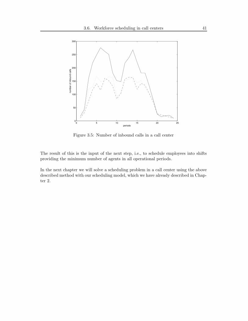
In the previous chapters we saw that such a center can be modeled as a queueingsystem. In case of call centers this model can be very complicated not only because ofthe complexity of a center but also due to the fluctuations of the calls (i.e., the load ofthe call center highly depends on time).In Figure 3.5 we plotted the number of incoming calls per period in a call center. Inthis plot one period is 30 minutes long and the operating hours are from 8 am to 8 pm.The three different plots represent different days of a week: Monday with normal line,Wednesday with dotted line and Friday with dashed line.As we can see the number of incoming calls not only differs from period to period butalso from day to day.

For measuring the service level in this environment it is common to use one of theformulas from the previous chapter (equation (3.10)-(3.13) for M/M/s queues andequations (3.20)-(3.25) for M/M/s/N queues). From these equations it is clear thatthe number of agents has effect on these performance metrics.In general we can say that all performance metrics are base on the Erlang formula oron one of its generalizations and thus these metrics are highly dependent on the agentnumber as well. To use one of these formulas we should estimate the load of the system.For this a common method is to divide the operating day into small periods (e.g., 15min., 30 min. or 1 hour) and calculate the aggregate load for each period. This can bedone by using historical data and mathematical tools. Based on these forecasted loadswe can compute the minimum number of agents for each period to reach the minimumservice level.

3.6. Workforce scheduling in call centers 41

0 5 10 15 20 250

50

100

150

200

250

300

periods

num

ber o

f inb

ound

cal

ls

Figure 3.5: Number of inbound calls in a call center

The result of this is the input of the next step, i.e., to schedule employees into shiftsproviding the minimum number of agents in all operational periods.

In the next chapter we will solve a scheduling problem in a call center using the abovedescribed method with our scheduling model, which we have already described in Chap-ter 2.

Chapter 4

An application in call centers

Up to this point we described the basic background for solving an agent schedulingproblem in call centers. In Chapter 1 we introduced the shift scheduling and the staffassigning problem and we analyzed some models from the literature. In Chapter 2 weintroduced and built up our workforce scheduling model, in which we model implicitlyshifts, i.e, with logical constraints. In Chapter 3 we gave a short survey about callcenters and queueing theory.

In this chapter we will solve an agent scheduling problem in call centers using our modelin Chapter 2 on page 29.

4.1 The scheduling environment

The scheduling environment chosen for this problem involves a continuous 8-hour workday from 9.00 to 17.00. Employee requirements are determined for 32 15-minute peri-ods i.e., our set P =

1, 2, 3, . . . , 31, 32

. In our model we have three different typesof employees: employees with a long term contract, part time employees and extraemployees, where all of the employees have single skill, i.e., K =

1

. We have differentrestrictions for each type of workers.For employees with a long term contract we have the following restrictions:

- they have to work in 6 hours shifts continually (including breaks),- each of them is given exactly one half-hour lunch break (2 consecutive periods)and one 15-minute coffee break,

- they have two separate break windows specified as follows:the start time of the lunch break window is specified as two hours afterthe starting period of the operating hours i.e.,the lunch break window is from 11.00 to 13.00,

- the coffee break window is from 14.00 to 16.00,- if an employee starts his/her work in one of the break windowsthen he/she will not receive break in that break window.

4.2. Input parameters 43

For part time employees we have possibilities for working, which were set up by them-selves, e.g., in case of call centers it is common that they fill in a form in the Internetand mark out exact periods, in which they can work. Moreover, they have to workcontinually in their working periods too.

For extra employees we do not have any constraints. We can interpret them in twodifferent ways.At the one hand, we can say that they are real employees with a rather high salary fora period and we only hire them for those periods, in which we could not satisfy therequirement. In other hand, we can interpret them as auxiliary variables; with themour model is always feasible. Because in our model the goal is to minimize the value ofthe objective function, we can avoid to use these employees by giving high cost to them(in our test problem we will follow this interpretation). In this way we can discoverunderstaffing and avoid it.

4.2 Input parameters

In our model there are input parameters, which we already described in Chapter 2.These parameters for our scheduling problem, which are contained inTable 4.1, are the following:

- the indexes of periods in the first column,- λp, i.e.,the number of call arrivals to the call center per minutefor each period in the second column,

- the number of required agents for each period in column three,- the exact requirements of part time employees for their working time,i.e., matrix A in columns 4-6,

- the optimal schedule for each employees with a long term contract,i.e., matrix S∗ in columns 7-19.

In our model we used consistent cost parameters for full time employees, part timeemployees and extra employees respectively. This means that

cpe = 100 ∀ p ∈ P,cpi = 2 ∀ p ∈ P, i ∈ Ic,cpi = 1 ∀ p ∈ P, i ∈ Ip.

Furthermore, we used the 80-20 service level metric, with 25 sec. average service time(i.e., β = 25 sec.) to calculate the number of required agents from the number ofincoming calls. This metric is defined as the following: 80% of costumers should beserved before 20 sec., i.e.,

P (wait < 20 sec.) = P (WQ < 20) = 1 − C(s, a)e−(s−a) 20β = 0.8 ,

where all of the notations were described in Chapter 3. To calculate these numbers weused the Erlang C calculator (http://www.math.vu.nl/ koole/ccmath/).

4.2. Input parameters 44

Part time

workers

Full time workers

Iop1 Apm2 Nora3 I. II. III. 1 2 3 4 5 6 7 8 9 10 11 12 13

1 1 2 1 0 1 1 0 1 0 0 0 0 0 0 0 1 1 02 2 2 1 0 1 1 0 1 0 0 0 0 0 0 0 1 1 03 2 2 1 1 1 1 0 1 0 0 0 0 0 0 0 1 1 04 4 3 1 1 1 1 0 1 0 0 0 0 0 0 0 1 1 05 15 8 1 1 1 1 0 1 1 1 0 0 0 0 0 1 1 06 22 11 1 1 1 1 0 1 1 1 0 0 0 1 0 1 1 07 24 12 1 1 1 1 0 1 1 1 0 0 0 1 0 1 1 08 27 13 1 1 1 1 0 1 1 1 1 0 0 1 0 1 1 19 22 11 1 1 1 1 0 1 1 1 1 0 0 1 0 1 1 110 19 10 1 1 0 1 0 1 1 1 1 0 0 1 0 1 1 111 25 12 1 1 1 1 0 1 1 1 1 0 0 1 0 1 1 112 28 14 1 1 1 1 1 1 1 1 1 0 0 1 0 1 1 113 24 12 1 1 1 1 1 1 1 1 1 0 0 1 0 1 1 114 20 10 1 1 1 1 1 1 1 1 1 0 1 1 0 1 1 115 15 8 1 1 1 1 1 1 1 1 1 0 1 1 1 1 1 116 15 8 1 0 1 1 1 1 1 1 1 1 1 1 1 1 1 117 24 12 1 1 1 1 1 1 1 1 1 1 1 1 1 1 1 118 25 12 1 1 1 1 1 1 1 1 1 1 1 1 1 1 1 119 31 15 0 1 1 1 1 1 1 1 1 1 1 1 1 1 1 120 26 13 1 1 1 1 1 1 1 1 1 1 1 1 1 1 1 121 29 14 1 1 1 1 1 1 1 1 1 1 1 1 1 1 1 122 23 11 1 1 1 1 1 1 1 1 1 1 1 1 1 1 1 123 17 9 1 1 1 0 1 1 1 1 1 1 1 1 1 1 1 124 24 12 1 1 1 0 1 1 1 1 1 1 1 1 1 1 1 125 20 10 0 1 1 0 1 1 1 1 1 1 1 1 1 1 1 126 17 9 0 0 0 0 1 1 1 1 1 1 1 1 1 1 1 027 18 9 0 0 0 0 1 1 1 0 1 1 1 1 1 1 1 028 9 5 0 0 0 0 1 1 1 0 1 1 1 1 1 0 0 029 10 6 0 0 0 0 1 1 0 0 1 1 1 0 1 0 0 030 7 4 0 0 0 0 1 1 0 0 0 1 1 0 1 0 0 031 6 4 0 0 0 0 1 1 0 0 0 1 1 0 1 0 0 032 1 2 0 0 0 0 1 0 0 0 0 1 1 0 1 0 0 0

1Index of periods2Arrivals per minute3Number of required agents

Table 4.1: Input parameters of the problem

4.3. The implementation of the model 45

4.3 The implementation of the model

In this section we deal with the way how we implemented our labor scheduling model.We describe techniques to represent nonlinear terms and to model different conditionswith logical constraints in our integer programming model.

4.3.1 The objective function in the model

In Subsection 2.4.3 we described the objective function of our model. From the defini-tion of d0(x, y) it is clear that the dM metric, which we use to express the preferencesof employees, is not linear. Even so, it is possible to represent this metric in an IPmodel. In the case when both x and y are 0, 1 variables, the discrete metric is

d0(x, y) = |x − y| =

0, if x = y,1, if x 6= y.

Using this result we get that dM (X,Y ) =∑

p,i vid0(Xpi, Ypi) =∑

p,i vi|Xpi − Ypi|. Oneof the commonly accepted ways to deal with absolute value function |x−y| in IP is thefollowing:

min δ, (4.1)

subject to

x − y ≤ δ, (4.2)

y − x ≤ δ, (4.3)

x, y, δ ∈ 0, 1 . (4.4)

We can see that in this representation δ is equivalent with the expression |x − y|. Inour model we followed this way to deal with the absolute value function.

4.3.2 Logical constraints in the model

One of the basic constraints is that all employees has to work continuously. For parttime employees we can implement this constraint with the following logical condition:if an employee does not work in a period and he/she worked in the previous one thenhe/she cannot work in the forthcoming periods. We can represent this constraints withexpression (2.9).For full time employees we also have this constraint but for them the implementation isdifferent because they have to work in 6 hours long shifts. Because of this, if they workin one period before the first break window then they have to work continuously untilthe beginning of the break window. We can model this condition with (2.16). We haveto model breaks for these employees, i.e., the first and the second relief breaks. We cando it with establish the following logical condition: if an employee worked before thefirst or the second break window than he/she has to have break in the break window.

4.4. Experimental results with the test problem 46

We can represent this constraint with using together inequality (2.9) and (2.16). Forthe lunch break we had to model also that its duration is 2 consecutive periods.Taken all round these are the main logical representations, which we used to implementour labor scheduling model.

4.4 Experimental results with the test problem

In this section we deal with the experimental results of our scheduling problem.We run different test problems with different combinations of weights, i.e., for w1, w2

and for vi. All of these problems were formulated in GAMS and we solved them us-ing the mixed integer programming option of GAMS with the OSL solver on a SunSparcstation with an Unix Solaris operating system. We created a formatted outputfrom the GAMS output to make the analysis easier. In this formated output we displaymatrix X = [X1 X2], the number of extra employees per periods, the number of agentsin periods and the number of required agents in periods. The value of the objectivefunction is also shown in our outputs. We divided this value into two parts; one is thecost of the schedule and one is the distance of the schedule from the ideal schedule S ∗.Both values are without the weight parameters w1 and w2.

In the first test problem the weights were the following:

w1 = 1,

w2 = 0,

vi = 1, i = 1, . . . , 13.

The result of this problem is shown in Table 4.3.With these parameters we wanted to minimize the cost of the schedule without payingany attention to the satisfaction of the agents, i.e., we ignored the metric part ofthe objective function by choosing w2 = 0. It is clear from the output that we donot need an extra employee in any period, which means that we satisfied the staffingrequirements.The maximum cost of any schedule is 100

∑

p np = 28500. This is the case when weonly hire extra employees for all periods. The cost of our schedule is 593, which isapproximately 2% of the worst case. It is important to see that our metric dependsalso on the values of vi, thus it is possible that for different vi we have distance in adifferent order of magnitude. The maximum distance between the ideal schedule S ∗

and the schedule with these parameters is 13× 32 = 416 and our result is 120, which isapproximately 29%. This ratio is not surprising because we ignored this part with theweight parameters.


In the second test problem we wanted to involve the preferences of the full time em-ployees, thus we chose the weights as

w1 = 1,

w2 = 1,

vi = 1, i = 1, . . . , 13.

The result of this test problem is shown in Table 4.4. In this result we also do not haveunder-staffing and we can see the big effect of the weights. We involved the metric partin the model with the same weight as the cost part and our result, in sense of agentssatisfaction, increase dramatically while the cost increased only slightly. The distancebetween the ideal schedule and our result is 88 and the cost of the schedule is 595 inthis case, which means that we improve the satisfaction by 8%, i.e., the new result is21% and the cost is only 595. In this test problem we can see the big effect of theweight parameters, with which we improved our results.

In the third test problem we wanted to make a distinction between full time employees.For this reason we changed the weight parameters of the problem. The parameters inthis case are

w1 = 1,

w2 = 1,

vi = 1, ∀ i 6= 1, 2, 3 ,

v1 = 2,

v2 = 2,

v3 = 2.

The result of the problem is in Table 4.5. In this case we avoid also to hire extraemployees and the cost of the schedule is 591. Because we changed the values of v1,v2 and v3 our metric result is not really comparable with the previous ones. Insteadof comparing the distance we can compare the number of no-hits in the results. Thismeans that we can calculate the number of non-identical elements between the solutionand the ideal schedule. This numbers are 120, 88 and 78 for the first, second and thirdtest problem respectively, which means that we improved the satisfaction of our em-ployees by changing the parameters. It is interesting to see that we not only improvedthe satisfaction of the employees, but with these parameters we were able to reduce thecost by 4, i.e., from 595 to 591.

In our fourth test problem we put larger accent to the metric part of the objectivefunction, which means that we wanted to satisfy the employees more than before. The


parameters of this problem are the following:

w1 = 1,

w2 = 5,

vi = 1, i = 1, . . . , 13.

The result of this test problem is shown in Table 4.6. In this case we made a schedulewithout under-staffing, with cost 593. It is clear from the output that we succeededin improving the satisfaction of the employees, i.e., we got 74 non-identical element inthe schedule, which is approximately 18%. In this case we can have nearly the sameconclusion as in the previous problem, namely that with these parameters we reducedthe number of non-identical elements between the ideal schedule and our result, mean-while the cost of the schedule remained approximately the same.

In our last test problem we used the following weight parameters:

w1 = 1,

w2 = 5,

vi = 1, ∀ i 6= 1, 2, 3 ,

v1 = 2,

v2 = 2,

v3 = 2.

The result of this problem is in Table 4.7. The cost of this schedule is 595, the distancefrom the ideal schedule is 97 and we avoid to hire extra employees again. It is also hardto compare the metric result with the other results because of the different vi weights.Even so we can compare the distance with the result in the third test problem becauseall vi are the same. In that case the distance was 101, which means that we improvedagain this performance measure.So far we made an analysis of the test problems and discussed some results. In Table4.2 all of the results are shown to make the comparison easier.

Number of non-identical elements

Problem w1 w2 vi Cost of schedule all Employee 1 Employee 2 Employee 3

1 1 0 id.1 593 120 19 14 102 1 1 id.1 595 88 15 10 103 1 1 non-id.2 591 78 11 2 104 1 5 id.1 593 74 11 4 105 1 5 non-id.2 595 74 11 2 10

1vi = 1, i = 1, . . . , 13.2vi = 1, ∀ i 6= 1, 2, 3 , v1 = 2 , v2 = 2, v3 = 2

Table 4.2: Results of the test problems


As we can see from Table 4.2 the cost of the schedules remained approximately thesame during our experiments but meanwhile we made an improvement in the satisfac-tory level. These results show us again how important it is to find a good combinationof weights. In the third test problem, where we made a distinction between employeesmeanwhile w1, w2 remained the same, we improved the satisfaction of the employeesby 10 and we improved the first and the second employee’s satisfaction with 4 and 8respectively, which means that we could find a right balance using these weights.In the last two cases, i.e., when we chose w2 = 5, the number of non-identical elementsbetween the ideal schedule and the result was 74 in both cases, which means that weincrease significantly the satisfaction of our employees.

After this analysis, in the next chapter we will make some concluding remarks about ourmodeling method, computational results and we will mention some future prospects.


Workforce scheduling model

rows - index of periods

1-13 - index of full time employees

I.,II.,III. - index of part time employees

EXTRA - number of extra employees in periods

AGENTS - number of agents in periods

NORA - number of required agents in periods

Cost of Schedule Distance from the optimal schedule

593 120

1 2 3 4 5 6 7 8 9 10 11 12 13 I.II.III. EXTRA AGENTS NORA

P1 0 0 0 0 0 0 0 0 0 0 0 0 0 1 0 1 0 2 2

P2 0 0 0 0 0 0 0 0 0 0 0 0 0 1 0 1 0 2 2

P3 0 0 0 0 0 0 0 0 0 0 0 0 0 1 0 1 0 2 2

P4 0 0 0 0 0 0 0 0 0 0 0 0 0 1 1 1 0 3 3

P5 0 1 0 1 1 0 1 0 0 1 1 1 0 1 1 1 0 10 8

P6 0 1 1 1 1 1 1 0 0 1 1 1 0 1 1 1 0 12 11

P7 0 1 1 1 1 1 1 0 0 1 1 1 0 1 1 1 0 12 12

P8 0 1 1 1 1 1 1 0 1 1 1 1 0 1 1 1 0 13 13

P9 0 1 1 1 0 1 1 0 1 0 1 1 0 1 1 1 0 11 11

P10 0 1 1 1 0 1 1 0 1 0 1 1 0 1 1 0 0 10 10

P11 1 1 1 1 1 0 1 1 1 1 1 1 1 1 1 1 0 15 12

P12 1 1 1 1 1 0 1 1 1 1 1 1 1 1 1 1 0 15 14

P13 1 1 0 1 1 1 0 1 1 1 1 1 1 0 1 1 0 13 12

P14 1 1 0 0 1 1 0 1 0 1 1 1 1 0 1 1 0 11 10

P15 1 0 1 0 1 1 1 1 0 1 0 0 1 0 1 1 0 10 8

P16 1 0 1 1 1 1 1 1 1 1 0 0 1 0 0 1 0 11 8

P17 1 1 1 1 1 1 1 1 1 1 1 1 1 0 1 1 0 15 12

P18 1 1 1 1 1 1 1 1 1 1 1 1 1 0 1 1 0 15 12

P19 1 1 1 1 1 1 1 1 1 1 1 1 1 0 1 1 0 15 15

P20 1 1 1 1 1 1 1 1 1 1 1 1 1 0 0 1 0 14 13

P21 1 1 1 1 1 1 1 1 1 1 1 1 1 0 0 1 0 14 14

P22 1 0 0 1 1 1 1 1 1 1 1 1 1 0 0 0 0 11 11

P23 1 1 1 0 1 1 1 1 1 0 1 0 1 0 0 0 0 10 9

P24 1 1 1 1 1 1 1 1 0 1 1 1 1 0 0 0 0 12 12

P25 1 1 1 1 0 0 1 1 1 1 1 1 1 0 0 0 0 11 10

P26 1 1 1 1 1 1 1 0 1 1 1 1 1 0 0 0 0 12 9

P27 1 1 1 1 1 1 1 1 1 1 0 1 0 0 0 0 0 11 9

P28 0 1 1 1 1 1 0 1 1 1 1 1 1 0 0 0 0 11 5

P29 1 0 1 0 0 1 0 1 1 0 0 0 1 0 0 0 0 6 6

P30 1 0 0 0 0 0 0 1 1 0 0 0 1 0 0 0 0 4 4

P31 1 0 0 0 0 0 0 1 1 0 0 0 1 0 0 0 0 4 4

P32 1 0 0 0 0 0 0 1 0 0 0 0 1 0 0 0 0 3 2

Table 4.3: Scheduling problem solution, with w1 = 1, w2 = 0 and vi = 1 i = 1, . . . , 13










595 88


P1 0 0 0 0 0 0 0 0 0 0 0 0 0 1 0 1 0 2 2

P2 0 0 0 0 0 0 0 0 0 0 0 0 0 1 0 1 0 2 2

P3 0 0 0 0 0 0 0 0 0 0 0 0 0 1 0 1 0 2 2

P4 0 0 0 0 0 0 0 0 0 0 0 0 0 1 1 1 0 3 3

P5 0 0 1 1 1 0 0 0 1 0 1 1 1 1 1 1 0 10 8

P6 0 1 1 1 1 0 0 0 1 0 1 1 1 1 1 1 0 11 11

P7 1 1 1 1 1 0 0 0 1 0 1 1 1 1 1 1 0 12 12

P8 1 1 1 1 1 1 0 1 1 0 1 1 1 1 1 1 0 14 13

P9 1 1 1 1 0 1 0 1 1 0 1 1 1 1 1 1 0 13 11

P10 1 1 1 1 0 1 0 0 1 0 1 0 1 1 1 0 0 10 10

P11 0 0 1 1 1 1 1 0 1 1 1 0 1 1 1 1 0 12 12

P12 0 0 1 1 1 1 1 1 1 1 1 1 1 1 1 1 0 14 14

P13 1 1 1 1 1 0 1 1 1 1 1 1 1 0 1 1 0 14 12

P14 1 1 1 0 1 0 1 1 1 1 1 1 0 0 1 1 0 12 10

P15 1 1 0 0 1 1 1 1 0 1 0 1 0 0 1 1 0 10 8

P16 1 1 0 1 1 1 1 1 0 1 0 1 1 0 0 1 0 11 8

P17 1 1 1 1 1 1 1 1 1 1 1 1 1 0 1 1 0 15 12

P18 1 1 1 1 1 1 1 1 1 1 1 1 1 0 1 1 0 15 12

P19 1 1 1 1 1 1 1 1 1 1 1 1 1 0 1 1 0 15 15

P20 1 1 1 1 1 1 1 1 1 1 1 1 1 0 1 1 0 15 13

P21 1 1 1 1 1 1 1 0 1 1 1 1 1 0 1 1 0 14 14

P22 1 1 1 1 1 1 1 1 1 1 1 1 1 0 0 0 0 13 11

P23 1 1 1 1 1 0 1 1 1 1 1 1 1 0 0 0 0 12 9

P24 1 1 1 1 1 1 1 1 0 1 1 1 1 0 0 0 0 12 12

P25 0 1 1 1 1 1 1 1 1 1 1 1 1 0 0 0 0 12 10

P26 1 0 1 0 1 1 1 1 1 1 1 1 1 0 0 0 0 11 9

P27 1 1 1 1 0 1 1 1 1 1 1 0 1 0 0 0 0 11 9

P28 1 1 0 1 1 1 0 1 1 0 0 1 0 0 0 0 0 8 5

P29 1 1 0 0 0 1 1 1 0 1 0 0 0 0 0 0 0 6 6

P30 1 0 0 0 0 1 1 1 0 1 0 0 0 0 0 0 0 5 4

P31 0 0 0 0 0 1 1 1 0 1 0 0 0 0 0 0 0 4 4

P32 0 0 0 0 0 0 1 0 0 1 0 0 0 0 0 0 0 2 2











591 101


P1 0 0 0 0 0 0 0 0 0 0 0 0 0 1 0 1 0 2 2

P2 0 0 0 0 0 0 0 0 0 0 0 0 0 1 0 1 0 2 2

P3 0 0 0 0 0 0 0 0 0 0 0 0 0 1 0 1 0 2 2

P4 0 0 0 0 0 0 0 0 0 0 0 0 0 1 1 1 0 3 3

P5 1 0 1 1 1 0 0 0 1 0 1 1 0 1 1 1 0 10 8

P6 1 0 1 1 1 1 0 0 1 0 1 1 1 1 1 1 0 12 11

P7 1 0 1 1 1 1 0 0 1 0 1 1 1 1 1 1 0 12 12

P8 1 0 1 1 1 1 0 1 1 1 1 1 1 1 1 1 0 14 13

P9 1 0 1 1 0 1 0 1 1 1 0 1 1 1 1 1 0 12 11

P10 1 0 1 1 0 1 0 1 1 1 0 0 1 1 1 0 0 10 10

P11 1 1 1 0 1 1 1 1 1 1 1 0 1 0 1 1 0 13 12

P12 1 1 1 0 1 1 1 1 1 1 1 1 1 0 1 1 0 14 14

P13 1 1 1 1 1 1 1 0 1 0 1 1 1 0 1 1 0 13 12

P14 0 1 1 1 1 1 1 0 1 0 1 1 1 0 1 1 0 12 10

P15 0 1 0 1 1 0 1 1 0 1 1 1 0 0 1 1 0 10 8

P16 1 1 0 1 1 0 1 1 0 1 1 1 0 0 0 1 0 10 8

P17 1 1 1 1 1 1 1 1 1 1 1 1 1 0 1 1 0 15 12

P18 1 1 1 1 1 1 1 1 1 1 1 1 1 0 1 1 0 15 12

P19 1 1 1 1 1 1 1 1 1 1 1 1 1 0 1 1 0 15 15

P20 1 1 1 1 1 1 1 1 1 1 1 1 1 0 1 0 0 14 13

P21 1 1 1 1 1 1 1 1 1 1 1 1 1 0 1 0 0 14 14

P22 1 1 0 1 1 0 1 1 1 1 1 1 1 0 0 0 0 11 11

P23 1 1 1 1 1 1 1 0 0 1 1 1 1 0 0 0 0 11 9

P24 1 0 1 1 1 1 1 1 1 1 1 1 1 0 0 0 0 12 12

P25 1 1 1 1 1 1 1 1 1 1 1 1 1 0 0 0 0 13 10

P26 0 1 1 1 1 1 1 1 1 1 1 1 0 0 0 0 0 11 9

P27 1 1 1 1 1 1 0 1 1 1 1 1 1 0 0 0 0 12 9

P28 1 1 1 0 0 1 1 1 1 0 0 0 1 0 0 0 0 8 5

P29 0 1 0 0 0 1 1 1 0 1 0 0 1 0 0 0 0 6 6

P30 0 1 0 0 0 0 1 1 0 1 0 0 0 0 0 0 0 4 4

P31 0 1 0 0 0 0 1 1 0 1 0 0 0 0 0 0 0 4 4

P32 0 1 0 0 0 0 1 0 0 0 0 0 0 0 0 0 0 2 2

Table 4.5: Scheduling problem solution, with w1 = 1, w2 = 1, vi = 1 ∀ i 6= 1, 2, 3,v1 = 2, v2 = 2 and v3 = 2










593 74


P1 0 0 0 0 0 0 0 0 0 0 0 0 0 1 0 1 0 2 2

P2 0 0 0 0 0 0 0 0 0 0 0 0 0 1 0 1 0 2 2

P3 0 0 0 0 0 0 0 0 0 0 0 0 0 1 0 1 0 2 2

P4 0 0 0 0 0 0 0 0 0 0 0 0 0 1 1 1 0 3 3

P5 1 0 0 1 1 0 0 0 0 0 1 1 1 1 1 1 0 9 8

P6 1 0 1 1 1 1 0 0 1 0 1 1 1 1 1 1 0 12 11

P7 1 0 1 1 1 1 0 0 1 0 1 1 1 1 1 1 0 12 12

P8 1 1 1 1 1 1 0 0 1 0 1 1 1 1 1 1 0 13 13

P9 1 0 1 1 1 1 0 0 1 0 1 1 1 1 1 1 0 12 11

P10 0 0 1 1 1 1 0 0 1 0 1 1 1 1 1 0 0 10 10

P11 0 1 1 1 1 0 1 1 1 1 1 1 1 1 1 1 0 14 12

P12 1 1 1 1 1 0 1 1 1 1 1 1 0 1 1 1 0 14 14

P13 1 1 1 1 0 1 1 1 1 1 1 1 0 0 1 1 0 13 12

P14 1 1 1 0 0 1 1 1 1 1 1 0 1 0 1 1 0 12 10

P15 1 1 0 0 1 1 1 1 0 1 0 0 1 0 1 1 0 10 8

P16 1 1 0 1 1 1 1 1 0 1 0 1 1 0 0 1 0 11 8

P17 1 1 1 1 1 1 1 1 1 1 1 1 1 0 1 1 0 15 12

P18 1 1 1 1 1 1 1 1 1 1 1 1 1 0 1 1 0 15 12

P19 1 1 1 1 1 1 1 1 1 1 1 1 1 0 1 1 0 15 15

P20 1 1 1 1 1 1 1 1 1 1 1 1 1 0 0 1 0 14 13

P21 1 1 1 1 1 1 1 1 1 1 1 1 1 0 0 1 0 14 14

P22 1 1 1 1 1 0 1 1 1 1 1 1 1 0 0 0 0 12 11

P23 1 1 1 0 1 1 1 1 1 1 1 1 1 0 0 0 0 12 9

P24 1 1 1 1 1 1 1 1 1 1 1 1 1 0 0 0 0 13 12

P25 1 1 1 1 1 1 1 1 1 1 1 1 1 0 0 0 0 13 10

P26 1 0 1 1 1 1 1 1 0 1 1 1 0 0 0 0 0 10 9

P27 1 1 1 1 1 1 1 1 1 1 1 1 1 0 0 0 0 13 9

P28 0 1 0 1 0 1 0 0 1 0 0 0 1 0 0 0 0 5 5

P29 0 1 1 0 0 1 1 1 1 1 0 0 0 0 0 0 0 7 6

P30 0 1 0 0 0 0 1 1 0 1 0 0 0 0 0 0 0 4 4

P31 0 1 0 0 0 0 1 1 0 1 0 0 0 0 0 0 0 4 4

P32 0 0 0 0 0 0 1 1 0 1 0 0 0 0 0 0 0 3 2











595 97


P1 0 0 0 0 0 0 0 0 0 0 0 0 0 1 0 1 0 2 2

P2 0 0 0 0 0 0 0 0 0 0 0 0 0 1 0 1 0 2 2

P3 0 0 0 0 0 0 0 0 0 0 0 0 0 1 0 1 0 2 2

P4 0 0 0 0 0 0 0 0 0 0 0 0 0 1 1 1 0 3 3

P5 1 0 0 1 1 0 0 0 1 0 1 1 1 1 1 1 0 10 8

P6 1 0 0 1 1 1 0 0 1 0 1 1 1 1 1 1 0 11 11

P7 1 0 1 1 1 1 0 0 1 0 1 1 1 1 1 1 0 12 12

P8 1 0 1 1 1 1 0 0 1 1 1 1 1 1 1 1 0 13 13

P9 1 0 1 1 1 1 0 0 1 1 1 1 1 1 1 1 0 13 11

P10 1 0 1 1 1 1 0 0 1 1 1 0 1 1 1 0 0 11 10

P11 1 1 1 1 1 1 1 1 1 1 0 0 1 1 1 1 0 14 12

P12 1 1 1 1 1 1 1 1 1 1 0 1 0 1 1 1 0 14 14

P13 1 1 1 1 1 1 1 1 0 0 1 1 0 1 1 1 0 13 12

P14 1 1 1 0 0 1 1 1 0 0 1 1 1 1 1 1 0 12 10

P15 0 1 0 0 0 0 1 1 1 1 1 1 1 0 1 1 0 10 8

P16 0 1 0 1 1 0 1 1 1 1 1 1 1 0 0 1 0 11 8

P17 1 1 1 1 1 1 1 1 1 1 1 1 1 0 1 1 0 15 12

P18 1 1 1 1 1 1 1 1 1 1 1 1 1 0 1 1 0 15 12

P19 1 1 1 1 1 1 1 1 1 1 1 1 1 0 1 1 0 15 15

P20 1 1 1 1 1 1 1 1 1 1 1 1 1 0 0 1 0 14 13

P21 1 1 1 1 1 1 1 1 1 1 1 1 1 0 0 1 0 14 14

P22 1 1 1 0 1 1 1 1 0 1 1 1 1 0 0 0 0 11 11

P23 1 0 0 1 1 0 1 1 1 1 1 1 1 0 0 0 0 10 9

P24 1 1 1 1 1 1 1 1 1 1 1 1 1 0 0 0 0 13 12

P25 1 1 1 1 1 1 1 1 1 1 1 1 1 0 0 0 0 13 10

P26 1 1 1 1 1 1 1 1 1 1 1 1 0 0 0 0 0 12 9

P27 0 1 1 1 0 1 1 1 1 1 1 1 1 0 0 0 0 11 9

P28 1 1 1 1 1 1 0 0 1 0 0 0 1 0 0 0 0 8 5

P29 0 1 1 0 0 1 1 1 0 1 0 0 0 0 0 0 0 6 6

P30 0 1 1 0 0 0 1 1 0 1 0 0 0 0 0 0 0 5 4

P31 0 1 0 0 0 0 1 1 0 1 0 0 0 0 0 0 0 4 4

P32 0 1 0 0 0 0 1 1 0 0 0 0 0 0 0 0 0 3 2

Table 4.7: Scheduling problem solution, with w1 = 1, w2 = 5, vi = 1 ∀ i 6= 1, 2, 3,v1 = 2, v2 = 2 and v3 = 2

Chapter 5

Concluding remarks and future

prospects

The main interest of this thesis was to introduce and apply a mathematical program-ming model for labor scheduling, which has the following properties:

1. it models implicitly shifts with logical constraints,

2. it solves the shift scheduling and the employee assignment problem together,

3. it models employees’ preferences.

In Chapter 2 we built up this model and introduced methods for express logical relation-ships between variables. We used several methods out of these during our experimentsto express specific conditions of the problem. We have already shown that it is pos-sible to express the same condition in different ways due to the equivalences, whichare shown in Section 2.2. This gives us an opportunity for the future to find the mostproper way to express different kinds of relationships in models and thus decrease thenumber of variables and constraints in the model.We defined a metric in Subsection 2.4.3 and used it to involve employees’ preferencesto the model. If we study the properties of this metric we can see that our choice wasrational. Of course it does not mean that this is the only way we can express thesepreferences. We can use different metrics or completely different expressions insteadof our metric. Fortunately, the change of this expression does not have big effect onthe structure of our modeling method, i.e., on the logical constraints. Even so, it ispossible that we use an expression, which is complicated to implement in an LP orIP environment. We described our method, with which we expressed the metric, inSubsection 4.3.1.

Our experimental results depends on both the implementation of the problem and theIP solver what we use. It can be very useful if we use other modeling techniques to solvethe problem. Using different logical implementations, different modeling techniques and

56

different solvers enables us to compare and analyze our results. This comparison andanalysis can be the next step in the future.

Bibliography

[1] Aykin, T. Optimal shift scheduling with multiple break windows. ManagementScience vol. 42 (1996), pp. 591–602.

[2] Bechtold, S. E., and Jacobs, L. W. The equivalence of set-covering and im-plicit optimal integer programming formulations for mathematical labor schedulingproblems. Tech. rep., Florida State University, 1989.

[3] Bechtold, S. E., and Jacobs, L. W. Implicit modelling of flexible break as-signments in optimal shift scheduling. Management Science vol. 36 (1990), pp.1339–1351.

[4] Dantzig, G. B. A comment on Edie’s traffic delays at toll booth. OperationsResearch vol. 2(3) (1954), pp. 339–341.

[5] Edie, L. C. Traffic delays at toll booths. Operations Research vol. 2 (1954), pp.107–138.

[6] Ernst, A. T., Jang, H., Krishnamoorthy, M., and Sier, D. Staff schedulingand rostering: A review of applications, methods and models. European Journal ofOperational Research vol. 153 (2004), pp. 3–27.

[7] Koole, G., and Mandelbaum, A. Queueing models of call centers. Annals ofOperations Research vol. 113 (2002), pp. 41–59.

[8] Thompson, G. M. Assigning telephone operators to shifts at New BrunswickTelephone Company. Interfaces vol. 27 (1997), pp. 1–11.

[9] Williams, H. P. Model Building in Mathematical Programming. Chichester Wiley,1998.

workforce scheduling with logical constraints: theory … · 2016-01-22 · chapter 1 models from...

Documents