worked examples from introductory physics vol. v: … examples from introductory physics vol. v:...

Worked Examples from Introductory PhysicsVol. V: Electric Currents and Magnetic Fields

David Murdock

Tenn. Tech. Univ.

August 19, 2004

Contents

To the Student. Yeah, You. i

1 Electric Current and Resistance 11.1 The Important Stuff . . . . . . . . . . . . . . . . . . . . . . . . . . . . . . . 1

1.1.1 Electric Current . . . . . . . . . . . . . . . . . . . . . . . . . . . . . . 11.1.2 Resistance & Ohm’s Law . . . . . . . . . . . . . . . . . . . . . . . . . 31.1.3 Dissipated Power . . . . . . . . . . . . . . . . . . . . . . . . . . . . . 4

1.2 Worked Examples . . . . . . . . . . . . . . . . . . . . . . . . . . . . . . . . . 41.2.1 Electric Current . . . . . . . . . . . . . . . . . . . . . . . . . . . . . . 41.2.2 Resistance & Ohm’s Law . . . . . . . . . . . . . . . . . . . . . . . . . 81.2.3 Dissipated Power . . . . . . . . . . . . . . . . . . . . . . . . . . . . . 9

2 DC Circuits 112.1 The Important Stuff . . . . . . . . . . . . . . . . . . . . . . . . . . . . . . . 11

2.1.1 Analyzing Circuits . . . . . . . . . . . . . . . . . . . . . . . . . . . . 112.1.2 Analyzing Circuits . . . . . . . . . . . . . . . . . . . . . . . . . . . . 122.1.3 Resistors in Series and in Parallel . . . . . . . . . . . . . . . . . . . . 142.1.4 Solving Big Messy DC Circuits . . . . . . . . . . . . . . . . . . . . . 152.1.5 RC Circuits. . . . . . . . . . . . . . . . . . . . . . . . . . . . . . . . . 15

2.2 Worked Examples . . . . . . . . . . . . . . . . . . . . . . . . . . . . . . . . . 172.2.1 Analyzing Circuits . . . . . . . . . . . . . . . . . . . . . . . . . . . . 172.2.2 Resistors in Series and in Parallel . . . . . . . . . . . . . . . . . . . . 172.2.3 Solving Big Messy DC Circuits . . . . . . . . . . . . . . . . . . . . . 172.2.4 RC Circuits. . . . . . . . . . . . . . . . . . . . . . . . . . . . . . . . . 17

3 Magnetic Fields – Forces 193.1 The Important Stuff . . . . . . . . . . . . . . . . . . . . . . . . . . . . . . . 19

3.1.1 Magnetic Fields . . . . . . . . . . . . . . . . . . . . . . . . . . . . . . 193.1.2 Magnetic Force on a Moving Point Charge. . . . . . . . . . . . . . . . 193.1.3 Circular Motion of Particles in Magnetic Fields . . . . . . . . . . . . 20

3.2 Worked Examples . . . . . . . . . . . . . . . . . . . . . . . . . . . . . . . . . 20

Appendix A: Useful Numbers 21

3

4 CONTENTS

To the Student. Yeah, You.

Hi. It’s me again. Since you have obviously read all the stuffy pronouncements about thepurpose of this problem–solving guide before, I won’t make them again here.

I will point out that I’ve got lots more work to do on Volume 5, and I’m just making itavailable so that these chapters (such as they are) may be of some help to you. In fact, thewhole set of books is a perpetual work in progress.

However....

Reactions, please!Please help me with this project: Give me your reaction to this work: Tell me what you

liked, what was particularly effective, what was particularly confusing, what you’d like tosee more of or less of. I can be reached at [email protected] or even at x–3044. If thiseffort is helping you to learn physics, I’ll do more of it!

DPM

i

ii TO THE STUDENT. YEAH, YOU.

Chapter 1

Electric Current and Resistance

1.1 The Important Stuff

1.1.1 Electric Current

The topics covered up to now in your physics course have dealt with concentrations of electriccharge which stay in one place, i.e. electrostatics. We now deal with the consequences ofcharge moving through a conductor, and the consequences are numerous, interesting andquite useful for modern technology. We now will work with electrodynamics.

In particular, we will study the flow of charge through electric circuits, i.e. networksof conductors, which might look like the one shown in Fig. 1.1.

In physics, we restrict this study to simple networks, focussing on the physical princi-ples involved; for complex networks involving exotic types of conductors, consult your localengineering department!

Charges moves through the different parts of a circuit; it is important to measure therate at which charge moves. Since charge cannot accumulate to any extent in the parts ofa circuit, if we look at any one branch of a circuit the same net number of charges will becrossing a cross-sectional area per unit time, as shown in Fig. 1.2. Note that in this figureI show positive charges doing the actual motion, which is not really the case for normalconductors; it is the negatively charged electrons which are in motion. However for all of our

+

_

C1

R1V0

R2

AcmeBatteries

Figure 1.1: Electric circuits!

1

2 CHAPTER 1. ELECTRIC CURRENT AND RESISTANCE

++++++

++++++

++++++++++++

++++++

++++++

++++++

++++++

++++++

++++++

++++++

++++++++++++

++++++

Figure 1.2: Current is the same in the skinny part of the wire as in the fat part; there are the same numberof charges crossing a cross-sectional area per time.

work it will not make any difference if we pretend that an equal number of positive chargeare moving in the direction opposite to that of the electron motion. We use this conventionbecause it was the one in use before it was known that negatively–charged electrons werethe ones that were in motion.

Suppose in a given branch of a circuit a small amount of charge dq passes through a givencross–sectional area in a time dt. Then the electric current in that branch is given by

I =dq

dt(1.1)

Of course, if the current is constant the we can use I = ∆q∆t

.From its definition in Eq. 1.1, electric current must have SI units of coulombs per second

(Cs) which is called an ampere1. Thus:

1 ampere = 1A = 1 Cs

.

Actually, we’ve seen this unit before (in Chapter 1) when we introduced the coulomb becauseit is actually the ampere which is easier to measure and standardize.

The definition of current involves a summation of the rates of passage of charges over theentire cross-sectional area, such as those in Fig. 1.2. Over any one tiny bit of this surface, ifthe density (number per volume) of charge carriers (with charge q) is n, and their averagespeed is vd (the drift velocity), then through some small area dA we get an electric currentdI given by

I = nqvdA . (1.2)

It is also useful to define a current density in the circuit branch. If the flow of chargesis uniform over the cross–sectional area, then the current density is

J =I

A(1.3)

which has units of Am2 .

Comparing Eq. 1.3 with Eq. 1.2 (and generalizing it to a vector equation) gives

J = nqvd (1.4)

so that the current density vector J points in the same direction as the mean drift velocityvd.

1Named in honor of the. . . uh. . . English physicist Jim Ampere (c.1835–1779) who did some electricalexperiments in. . . um. . .Heidelberg. That’s it, Heidelberg.

1.1. THE IMPORTANT STUFF 3

1.1.2 Resistance & Ohm’s Law

Current flows in a conductor when an electric potential is applied across its ends. What is therelation between the amount of current flowing (I) and the potential difference (“voltage”,V )? Empirically, it is found that for “normal” materials, the current through a conductor isproportional the potential difference applied across its ends: I ∝ V . The ratio of voltage tocurrent is the resistance of the conductor:

R =V

I(1.5)

which is the same as:V = IR (1.6)

and is known as Ohm’s Law.Resistance is a scalar quantity and from Eq. 1.5 has units of Volt

Coul, which is called an

ohm2. Thus:

1 ohm = 1Ω = 1volt

ampere

The resistance of a particular conductor depends on the material of which it is made andits size and shape. For a simple shape like a cylinder (with electrical leads attached to theends), we have a simple expression for the resistance. It is

R = ρL

A(1.7)

where L is the length of the conductor and A is its cross-sectional area. The proportionalityconstant ρ depends on the material from which the conductor is made. From its definitionwe see that ρ must have units of Ω · m. For example,

ρCopper = 1.69 × 10−8 Ω · mρAluminum = 2.75 × 10−8 Ω · m

Actually, the real definition of resistivity comes from a more general version of Ohm’sLaw which relates the electric field (vector) within the conductor to the current density(vector):

E = ρJ (1.8)

The resistance of a certain conductor can also depend on its temperature. While thisdependence might not be important for some conductors it can be important for those caseswhere a conductor is (intentionally!) heated to very large temperatures. Empirically it isfound that a linear dependence of R on T (Celsius or Kelvin; it doesn’t matter for a generallinear relation) works pretty well, and we use a relation of the form:

ρ − ρ0 = ρ0α(T − T0) R − R0 = R0α(T − T0) (1.9)

2Named in honor of the. . . uh. . .Polish physicist Jim Ohm (1215–1492) who did some electrical experi-ments in. . . um. . .Prague. That’s it, Prague.


1.1.3 Dissipated Power

As an amount of charge dq passes through a resistor it “sees” a change in electrical potentialIR and thus a change in electrical potential energy (IR)dq. The energy lost by the chargegoes into the thermal energy of the resistor since energy is never really lost.

If dt is the time over which this charge dq has passed through the resistor then the rateat which energy is being “lost” in the resistor (the dissipated power, P ) is

P =IR dq

dt= IR(I) = I2R

where we used dqdt

= I. Since IR is the voltage drop across the resistor, we can also writethis as P = V I. Thus we have:

P = IV = I2R =V 2

R(1.10)

We have already encountered the quantity power in the mechanics part of these notes. Thereis was defined as work done per time (energy per time, same as here) and the SI unit ofpower was given as J

s, also known as the watt3

1.2 Worked Examples

1.2.1 Electric Current

1. A current of 5.0A exists in a 10Ω resistor for 4.0min. How many (a) coulombsand (b) electrons pass through any cross section of the resistor in this time?

(a) Using the constant–current version of Eq. 1.1, (namely I = ∆q∆t

), for the given current Iand time interval ∆t we get:

∆q = I∆t = (5.0A)(4.0min)(

60 s

1min

)

= 1.2 × 103 C

So 1.2 × 103 coulombs pass through any cross section of the wire in 4.0min.

(b) In part (a) we have found the absolute value of the electric charge passing through anypart of the wire; to find the number of electrons which make up this charge, divide this bythe absolute value of the electron charge e:

N =∆q

e=

(1.2 × 103 C)

(1.602 × 10−23 C)= 7.5 × 1021 electrons

3Named in honor of the. . . uh. . . Scottish physicist Jim Watt (1736–1819) who did some mechanical ex-periments in. . . um. . . Glasgow. That’s it, Glasgow.

1.2. WORKED EXAMPLES 5

2. In a particular cathode ray tube, the measured beam current is 30µA. Howmany electrons strike the tube screen every 40 s?

Here, I is constant (and as used here it gives the magnitude of the flow of charge) so theamount of charge which strikes the screen has a magnitude

∆q = I∆t = (30 × 10−6 A)(40 s) = 1.2 × 10−3 C ,

that is, a total charge of −1.2 × 10−3 C (since it is electrons which move in the tube) hitsthe screen. Use the charge per electron to find the number of electrons:

N = (−1.2 × 10−3 C)

(1 electron

−1.60 × 1019 C

)= 7.5 × 1015 electrons

3. Suppose that the current through a conductor decreases exponentially withtime according to

I(t) = I0e−t/τ

where I0 is the initial current (at t = 0), and τ is a constant having dimensions oftime. Consider a fixed observation point within the conductor. (a) How muchcharge passes this point between t = 0 and t = τ? (b) How much charge passesthis point between t = 0 and t = 10τ? (c) How much charge passes this pointbetween t = 0 and t = ∞?

(a) The relation between charge increment dq and time increment dt can be written usingEq. 1.1 as:

dq = idt = I0e−t/τdt .

To sum up all the charge passing a point between t = 0 and t = τ , do the integral on timeto get:

q =∫ τ

0i(t) dt =

∫ τ

0I0e

−t/τ dt

= −I0τe−t/τ

∣∣∣∣τ

0= −I0τ

(e−1 − 1

)

= I0τ (1 − e−1) = (0.623)I0τ

(b) For the charge passing the observation point between t = 0 and t = 10τ do the sameintegral as in (a) but from 0 to 10τ :

q =∫ 10τ

0I0e

−t/τ dt

= −I0τe−t/τ

∣∣∣∣10τ

0= −I0τ

(e−10 − 1

)

= I0τ (1 − e−10) = (0.9995)I0τ


(c) Now do the same integral, but from 0 to ∞:

q =∫ ∞

0I0e

−t/τ dt

= −I0τe−t/τ

∣∣∣∣∞

0= −I0τ (0 − 1)

= I0τ = I0τ

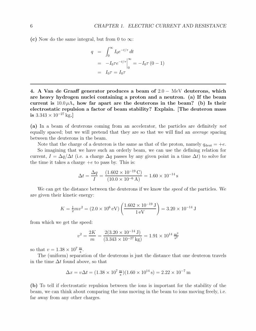
4. A Van de Graaff generator produces a beam of 2.0 − MeV deuterons, whichare heavy hydrogen nuclei containing a proton and a neutron. (a) If the beamcurrent is 10.0µA, how far apart are the deuterons in the beam? (b) Is theirelectrostatic repulsion a factor of beam stability? Explain. [The deuteron massis 3.343 × 10−27 kg.]

(a) In a beam of deuterons coming from an accelerator, the particles are definitely notequally spaced; but we will pretend that they are so that we will find an average spacingbetween the deuterons in the beam.

Note that the charge of a deuteron is the same as that of the proton, namely qdeut = +e.So imagining that we have such an orderly beam, we can use the defining relation for

current, I = ∆q/∆t (i.e. a charge ∆q passes by any given point in a time ∆t) to solve forthe time it takes a charge +e to pass by. This is:

∆t =∆q

I=

(1.602 × 10−19 C)

(10.0 × 10−6 A)= 1.60 × 10−14 s

We can get the distance between the deuterons if we know the speed of the particles. Weare given their kinetic energy:

K = 12mv2 = (2.0 × 106 eV)

(1.602 × 10−19 J

1 eV

)= 3.20 × 10−14 J

from which we get the speed:

v2 =2K

m=

2(3.20 × 10−14 J)

(3.343 × 10−27 kg)= 1.91 × 1014 m2

s2

so that v = 1.38 × 107 ms.

The (uniform) separation of the deuterons is just the distance that one deuteron travelsin the time ∆t found above, so that

∆x = v∆t = (1.38 × 107 ms)(1.60 × 1014 s) = 2.22 × 10−7 m

(b) To tell if electrostatic repulsion between the ions is important for the stability of thebeam, we can think about comparing the ions moving in the beam to ions moving freely, i.e.far away from any other charges.


The potential energy of a pair of deuterons separated by the distance found above (ascompared with their energy at infinite separation) is

Uelec = ke2

∆x=(8.99 × 109 N·m2

C2

) (1.60 × 10−19 C)2

(2.22 × 10−7 m)

= 1.04 × 10−21 J = 6.5 × 10−3 eV

which is much smaller than the kinetic energy of the particles, which is of the order of MeV’s.We can guess from this that the motion of the deuterons in this beam is not much differentfrom that of free particles and the stability of beam is not influenced (much) by the mutualrepulsion of the ions.

5. Calculate the average drift speed of electrons travelling through a copper wirewith a cross-sectional area of 1.00mm2 when carrying a current of 1.00A (valuessimilar to those for he electric wire to your study lamp). It is known that aboutone electron per atom of copper contributes to the current. The atomic weightof copper is 63.54, and its density is 8.92 g/cm3

Eventually, we’ll get vd from Eq. 1.2, I = nqvdA, so first we find n, the number densityof freely-moving electrons in the wire. Now the mass density of copper is

ρ = 8.92 gcm3 = 8.92 × 103 kg

m3

and using the atomic weight (0.06354 kg for each mole) and Avogadro’s number we can getthe number density of coper atoms:

nCu = 8.92 × 103 kgm3

(1mole

0.06354 kg

)(6.022 × 1023 atoms

mole

)

= 8.454 × 1028 atomm3

Now since there is only one electron for each copper atom that contributes to the currenti.e. is freely–moving), then the number density of the conduction electrons is also n =8.454 × 1028 m−3.

Now use Eq. 1.2 to get the drift speed. Assume that the total current 1.00A = 1.00 Cs

is uniform over the cross-sectional area, and use the magnitude of the charge of the carriersq = e = 1.60 × 10−19 C and get:

vd =I

nqA

=(1.00 C

s)

(8.454 × 1028 m−3)(1.60 × 10−19 C)(1.00 × 10−6 m3)= 7.4 × 10−5 m

s

The drift speed of the electrons is 7.4 × 10−5 ms. . . a rather small speed!


1.2.2 Resistance & Ohm’s Law

6. A conducting wire has a 1.0mm diameter, a 2.0m length, and a 50mΩ resistance.What is the resistivity of the material?

The cross-sectional area of the wire is

A = πr2 = πd2

4= π

(1.0 × 10−3 m)2

4= 7.85 × 10−7 m2

Then from Eq. 1.7 the resistivity ρ is given by

ρ =RA

L

=(50 × 10−3 Ω)(7.85 × 10−7 m2)

(2.0m)= 2.0 × 10−8 Ω ·m

7. A steel trolley-car wire has a cross-sectional area of 56.0 cm2. What is theresistance of 10.0 km of rail? The resistivity of the steel is 3.00 × 10−7 Ω · m.

We have the resistivity ρ, cross-sectional area and length. (Note that 1 cm2 = 10−4 m2 !)Then Eq. 1.7 gives the resistance of the rail:

R = ρL

A= (3.00 × 10−7 Ω · m)

(10.0 × 102 m)

(56.0 × 10−4 m2)= 0.536Ω

8. When 115V is applied across a wire that is 10m long and has a 0.30mm radius,the current density is 1.4 × 104 A/m2. Find the resistivity of the wire.

By doing some algebra first we can save ourselves some button-pushing. Write out Ohm’slaw and substitute for the resistance R:

V = IR = I(ρL

A

)

=(

I

A

)ρL = JρL

where we’ve also used the definition of the current density, J = I/A, since we are given itsvalue. Solve for ρ and plug in the numbers:

ρ =V

JL=

(115V)

(1.4 × 104 A/m2)(10m)= 8.2 × 10−4 Ω · m

So the resistivity of the wire is 8.2 × 10−4 Ω · m.


As it turns out, we did not need to know the radius of the wire.

9. A common flashlight bulb is rated at 0.30A and 2.9V (the values of the currentand voltage under operating conditions). If the resistance of the bulb filament atroom temperature (20C) is 1.1Ω, what is the temperature of the filament whenthe bulb is on? The filament is made of tungsten, for which α = 4.5 × 10−3/K.

From Ohm’s law we can find the resistance of the bulb at the temperature of the normaloperating conditions (hot!):

R =V

I=

(2.9V)

(0.30A)= 9.7Ω

This is in contrast to the resistance of the filament at room temperature, 1.1Ω.Equation 1.9 gives the dependence of resistivity (ρ) on temperature. The same relation

holds true for the resistance R of a circuit element because to get R from ρ we multiply byL/A (assume a cylindrical conductor). So we use

R − R0 = R0α(T − T0)

with our values for T0 = 20C and solve for T . We get:

(T − T0) =1

α

(R − R0)

R0=

1

(4.5 × 10−3/K)

(9.7Ω − 1.1Ω)

1.1Ω= 1.7 × 103 K = 1.7 × 103 C

Then the operating temperature T is

T = T0 + 1.7 × 103 C = 20C + 1.7 × 103 C = 1.7 × 103 C

1.2.3 Dissipated Power

10. A certain x-ray tube operates at a current of 7.0 [mA and a potential differenceof 80 kV. What is its power in watts?

The problem gives us the current I passing through the tube and the potential difference(voltage drop) V across the tube. Then Eq. 1.10 gives us the power dissipated:

P = IV = (7.0 × 10−3 A)(80 × 103 V) = 5.6 × 102 W

11. Thermal energy is produced in a resistor at a rate of 100W when the currentis 3.00A. What is the resistance?

Here we are given the power dissipated in the resistor and the current passing throughit. Then we can get the resistance by using P = I2R. This gives:

R =P

I2=

(100W)

(3.00A)2= 11.1Ω

Chapter 2

DC Circuits


2.1.1 Analyzing Circuits

We now extend the ideas of the last chapter to situations where circuit elements (such asbatteries and resistors) are attached together in more complicated (and interesting!) ways.We will look at circuits with multiple loops and calculate the important quantities for thesecircuits: The potential differences between various points in the circuit and the currentsflowing in the different branches of the circuit. For example, we might be given a circuit,part of which may look like the one shown in Fig. 2.1. Given the values of V and R1, R2, . . .it would be our job to find the currents in the different branches, i1, i2 . . . and perhaps thepotential difference between the points a and b.

There is an important point to be made about the direction of the arrow we put in ourpictures and the actual direction in which current is flowing: For the sake of getting ourselvesstraight, we might begin a circuit problem by writing down arrows to reference the directionsof the currents as in Fig. 2.1. But we may later find that one of the i’s is negative! That’snot a problem; it only means that we guessed wrong for the direction of the current in one

a

b

i1

i5

i2

i4i3

R1

R4

R5 R3

R2

V

Figure 2.1: Analyzing a circuit: What are the currents i1, i2, . . . ? What is the potential difference betweenthe points a and b ?

11

12 CHAPTER 2. DC CIRCUITS

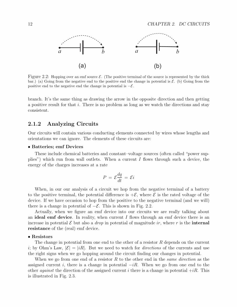
a b a b

(a) (b)

Figure 2.2: Hopping over an emf source E . (The positive terminal of the source is represented by the thickbar.) (a) Going from the negative end to the positive end the change in potential is E . (b) Going from thepositive end to the negative end the change in potential is −E .

branch. It’s the same thing as drawing the arrow in the opposite direction and then gettinga positive result for that i. There is no problem as long as we watch the directions and stayconsistent.


Our circuits will contain various conducting elements connected by wires whose lengths andorientations we can ignore. The elements of these circuits are:

• Batteries; emf Devices

These include chemical batteries and constant–voltage sources (often called “power sup-plies”) which run from wall outlets. When a current I flows through such a device, theenergy of the charges increases at a rate

P = E dq

dt= Ei

When, in our our analysis of a circuit we hop from the negative terminal of a batteryto the positive terminal, the potential difference is +E, where E is the rated voltage of thedevice. If we have occasion to hop from the positive to the negative terminal (and we will)there is a change in potential of −E. This is shown in Fig. 2.2.

Actually, when we figure an emf device into our circuits we are really talking aboutan ideal emf device. In reality, when current I flows through an emf device there is anincrease in potential E but also a drop in potential of magnitude ir, where r is the internalresistance of the (real) emf device.

• ResistorsThe change in potential from one end to the other of a resistor R depends on the current

i; by Ohm’s Law, |E| = |iR|. But we need to watch for directions of the currents and usethe right signs when we go hopping around the circuit finding our changes in potential.

When we go from one end of a resistor R to the other end in the same direction as theassigned current i, there is a change in potential −iR. When we go from one end to theother against the direction of the assigned current i there is a change in potential +iR. Thisis illustrated in Fig. 2.3.


a b a bi i

(a) (b)

Figure 2.3: Hopping over a resistor R. (a) Going from a to b along with the assigned direction of thecurrent, the change in potential is −iR. (b) Going from a to b against the assigned direction of the current,the change in potential is +iR. Note, we are not saying that i is positive here.

C

i

q -q

a b

Figure 2.4: Hopping over a capacitor C in the analysis of a circuit. Going from a to b with the chargeof the capacitor q defined as shown, there is a change in potential − q

C . Charge q is related to current i byi = dq

dt .

• Capacitors

We will encounter capacitors again when we discuss circuits where we switch on thecontact between a capacitor’s plates and a battery (with a resistance in the circuit); we willstudy how the current into the plates (and the charge on the plates) changes with time.Recall that from our old formula q = CV (that is, V = q/C) when we go from the platewith charge q to the plate with charge −q, the change in potential is −q/C, as illustrated inFig. 2.4.

• Inductors

Whoa! We haven’t encountered these yet, and for the time being we won’t put them inour circuits! We need to study magnetic fields to understand what an inductor does!

However, for the record, an inductor is a coil of wire, the potential drop across a inductordepends on the rate of change of the current and is given by +Ldi

dt. L is the measure of the

property called “self–inductance” and is measured in Henrys. But we’ll get to that later on.

We use these rules for finding potential differences along with two facts:

• The sum of the potential differences taken around any closed loop in a circuit must bezero.

• The sum of the currents entering any junction must equal the sum of the currents exitingthat junction. Then we can find all the currents if we just work hard enough.


R1

R5

R6

R4

R2

R3

(a) (b)

Figure 2.5: (a) Resistors R1, R2 and R3 are connected in series. (b) Resistors R4, R5 and R6 are connectedin parallel.

a bR1 R2

Rn= a b

Req

i i

V V

Figure 2.6: A set of resistors R1, R2, . . .Rn connected in series has a current i common to all the resistorsand a potential drop V across the whole set. For the purposes of finding the current i, it can be treated asa single equivalent resistor given by Req = R1 + R2 + . . . + Rn. Then V = iReq.

These rules are known as the Kirchhoff loop rule and the Kirchhoff junction rule,respectively. It is necessary to use them when we have to analyze a circuit with multipleloops.

2.1.3 Resistors in Series and in Parallel

Oftentimes in a circuit we have a set of resistors joined together either by connecting themend-to-end (a series connection) or by connecting both of their ends together (a parallelconnection). The two types of connections are illustrated in Fig. 2.5.

When we have resistor combinations like these, we can take some shortcuts in our analysisof the circuit; we can treat the set as a single equivalent resistor, at least as far as the currententering the set is concerned.

• Series Combination

Suppose we have a set of resistors in a string, with values R1, R2, ...Rn; the resistors arejoined end–to–end with no other connections made between the resistors in the string. Thenthe resistors can be replaced the equivalent resistance Req given by

Req = R1 + R2 + . . . Rn (2.1)

This substitution in diagrammed in Fig. 2.6.

• Parallel Combination


R1 R2 Rn

a

b

i

i

V Req

a

b

i

i

V=

Figure 2.7: A set of resistors R1, R2, . . .Rn connected in parallel has a potential difference V common toall the resistors. A total current i enters and exits the combination. For the purposes of finding this currentit can be treated as a single equivalent resistor given by R−1

eq = R−11 + R−1

2 + . . . + R−1n . Then V = iReq.

Suppose we have a set of resistors with values R1, R2, ...Rn; the ends of these resistorsare joined together. Then the resistors can be replaced the equivalent resistance Req givenby

1

Req=

1

R1+

1

R2+ . . .

1

Rn(2.2)

This substitution in diagrammed in Fig. 2.7.In the special case where we have only two resistors R1 and R2 in parallel, the formula

gives:1

Req=

1

R1+

1

R2=

R1 + R2

R1R2

so then

Req =R1R2

(R1 + R2)(2.3)

2.1.4 Solving Big Messy DC Circuits

Big messy DC circuits can be solved by applying the Kirchhoff rules to get a set of independentlinear equations for the unknown currents and then solving them for the currents in theseparate branches.

• In each branch of the circuits assign a current, including a direction; draw a labelled arrowon the diagram for each current.

••••

2.1.5 RC Circuits.

Now we have a look at a circuit in which the current is not constant. (More will follow!)We consider the circuit shown in Fig. 2.8. The circuit has a resistor R and a capacitor C


a

b

SR

CE

Figure 2.8: RC circuit; with the switch thrown to position a the capacitor C builds up a charge. Thenwith the switch thrown to b the capacitor discharges.

connected in series. Depending on whether the switch in thrown to a ro b we can include ornot include a battery with emf E is series with them.

Suppose the capacitor is initially uncharged and at time t = 0 the switch is thrown to a.One can show that the charge on the capacitor is given by

q(t) = CE(1 − e−t/(RC)) (2.4)

and the current in the circuit is

i(t) =dq

dt=( E

R

)e−t/(RC) (2.5)

The combination RC that occurs in both of these results has units of time. We represent itby the symbol τ :

τ = RC . (2.6)

τ is called the capacitive time constant for the circuit.Eq. 2.4 tells us that at very “large” values of t the exponential term is very small and

so the charge q is very nearly equal to CE. This is the “full”, or equilibrium value of thecharge on the capacitor. The value of q at a time t = τ after we close the switch turns outto be about 0.63 (i.e. 63%) of this value, so that τ gives a measure of the time required for“most” of the equilibrium charge to collect.

Eq. 2.5 tells us that the current starts off with the value ER

(the value it would have ifthere were no capacitor in the circuit) and it falls off to zero at large values of t. At t = τthe current has decreased to about 37% of its initial value.

Now when we throw the switch to position b (at t = 0) the capacitor will lose its chargeas the current goes the opposite way through the resistor (this time bypassing the battery).One can show that the charge on the capacitor is given by

q(t) = q0e−t/(RC) (2.7)


where q0 was the charge on the capacitor when the switch was thrown to b. The current inthe circuit is now:

i(t) =dq

dt= −

(q0

RC

)e−t/(RC) (2.8)

(note, the minus sign tell us that the current flows the opposite way from the direction ithad when C was charging).

2.2 Worked Examples


2.2.2 Resistors in Series and in Parallel

2.2.3 Solving Big Messy DC Circuits

2.2.4 RC Circuits.

Chapter 3

Magnetic Fields – Forces


3.1.1 Magnetic Fields

Just as a charge q experiences a force F = qE from an electric field E (whether or not it is inmotion), a moving charge q will experience a new kind of force if it is moving in a magneticfield.

The magnetic field is given the symbol B, and like the electric field, it is a vector field,that is, at each point in space its value is specified by giving its three components (or byits direction and magnitude). As with electric fields, we can get a useful overall picture of amagnetic field by showing magnetic field lines; these give the direction of the B field at eachpoint but not the magnitude.

The magnetic field B is measured in tesla; more on that in the next section.

3.1.2 Magnetic Force on a Moving Point Charge.

When a point charge q moves with velocity v in a magnetic field B, it experiences a forcewhich is proportional to both the charge’s speed and the magnitude of the field, but thedirection of the force is perpendicular to both v and B. Furthermore, for a nonzero force, Bmust have a component perpendicular to v; if the velocity is parallel to B there is no force.

If the angle between v and B is θ, then the magnitude of the magnetic force is

F = |q|vB sin θ

and the direction of the force is given by the right hand rule: Point your four fingers inthe direction of v and let them sweep (bend) from v to B. Then your thumb points in thedirection of the force F, if q is positive. If q is negative, F points in the opposite direction.

The force law given above is neatly expressed using the cross product:

F = qv × B (3.1)

19

20 CHAPTER 3. MAGNETIC FIELDS – FORCES

As mentioned above, the magnetic field is measured in Tesla1.

3.1.3 Circular Motion of Particles in Magnetic Fields

If a particle enters a uniform magnetic field having a velocity perpendicular to the directionof the field it will undergo circular motion; the centripetal force is provided by the magneticforce.

Recall that a particle undergoes circular motion because there is a force pulling it towardthe center of the circle. The centripetal force is perpendicular to the velocity and hasmagnitude mv2/r where r is the radius of the circle. Here, the centripetal force is suppliedby the magnetic force; since the velocity is perpendicular to the field, the magnetic force hasmagnitude qvB, where q is he absolute value of the charge of the particle. Equating the twoexpressions and cancelling a factor of v gives:

qB =mv

r(3.2)

3.2 Worked Examples

1Named in honor of the. . . uh. . . Swedish physicist Jim Tesla (1935–2021) who did some electrical experi-ments in. . . um. . . Zurich. That’s it, Zurich.

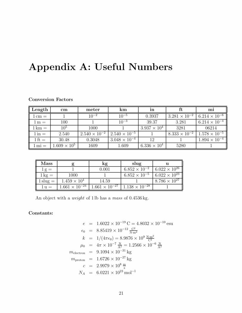
Appendix A: Useful Numbers

Conversion Factors

Length cm meter km in ft mi

1 cm = 1 10−2 10−5 0.3937 3.281 × 10−2 6.214 × 10−6

1m = 100 1 10−3 39.37 3.281 6.214 × 10−4

1 km = 105 1000 1 3.937 × 104 3281 062141 in = 2.540 2.540 × 10−2 2.540 × 10−5 1 8.333 × 10−2 1.578 × 10−5

1 ft = 30.48 0.3048 3.048 × 10−4 12 1 1.894 × 10−4

1mi = 1.609 × 105 1609 1.609 6.336 × 104 5280 1

Mass g kg slug u1 g = 1 0.001 6.852 × 10−2 6.022 × 1026

1 kg = 1000 1 6.852 × 10−5 6.022 × 1023

1 slug = 1.459 × 104 14.59 1 8.786 × 1027

1 u = 1.661 × 10−24 1.661 × 10−27 1.138 × 10−28 1

An object with a weight of 1 lb has a mass of 0.4536 kg.

Constants:

e = 1.6022 × 10−19 C = 4.8032 × 10−10 esu

ε0 = 8.85419 × 10−12 C2

N·m2

k = 1/(4πε0) = 8.9876 × 109 N·m2

C2

µ0 = 4π × 10−7 NA2 = 1.2566 × 10−6 N

A2

melectron = 9.1094 × 10−31 kg

mproton = 1.6726 × 10−27 kg

c = 2.9979 × 108 ms

NA = 6.0221 × 1023 mol−1

21

worked examples from introductory physics vol. v: … examples from introductory physics vol. v:...

Documents