work-life balance and labor force attachment at older...
TRANSCRIPT

Work-Life Balance and Labor Force Attachment at Older Ages
Marco Angrisani University of Southern California
Maria Casanova
California State University, Fullerton
Erik Meijer University of Southern California
Prepared for the 19th Annual Joint Meeting of the Retirement Research Consortium August 3-4, 2017 Washington, DC
The research reported herein was pursuant to a grant from the U.S. Social Security Administration (SSA), funded as part of the Retirement Research Consortium. The findings and conclusions expressed are solely those of the authors and do not represent the views of SSA, any agency of the federal government, the University of Southern California, California State University, Fullerton, or the University of Michigan Retirement Research Center.

1 Introduction
Demographic trends over the last five decades have led to longer life expectancies and declin-
ing birth rates. The resulting concerns about the long-term sustainability of Social Security
programs have focused attention on understanding what drives individuals’ retirement deci-
sions and on how to increase older workers’ labor force attachment (Wise, 2010). Tradition-
ally, economists have focused on monetary incentives such as Social Security rules (Gruber
and Wise, 2004; French, 2005), private pension arrangements (Lumsdaine and Mitchell,
1999), and the availability of health insurance (French and Jones, 2011). Health shocks have
been recognized as further determinants of the relative (dis)utility of work versus retirement
(Currie and Madrian, 1999; McGeary, 2009), as have non-monetary characteristics of the
job environment (Angrisani et al., 2017, 2015).
A growing literature has identified work-life balance (WLB), defined as the absence of
conflict between work and non-work activities, as a key determinant of workers’ evaluation
of the relative attractiveness of work versus leisure, particularly at older ages (Bianchi and
Milkie, 2010; Gardiner et al., 2007; Guest, 2002; Raymo and Sweeney, 2006). Workers whose
jobs allow them to more easily manage their private life (children, doctor visits, caring for
an elderly parent or sick spouse, etc.) may be more likely to remain employed than those
who perceive that their jobs interfere with their personal lives.
A better understanding of the effect of WLB on retirement behavior, and of the specific
life circumstances during which WLB becomes valuable to employees, provides a policy
handle to affect workplace arrangements so as to facilitate longer labor force attachment at
older ages. This line of research is particularly timely in view of the increase in women’s labor
force participation in the past decades, which has led to a growing number of female workers
on the verge of retirement. Because of existing social norms related to gender roles, women
are typically more sensitive to the trade-off between career and family life (Lewis, 2008).
At the same time, late fertility and longer life expectancy have placed more responsibility
on middle-age/older workers for supporting their own children and caring for their aging
parents, thus increasing the strain on WLB.
In this paper, we use data from the Health and Retirement Study (HRS) to investigate
the relationship between WLB and retirement transitions. We use a sample of workers aged
51 to 79 to assess the extent to which WLB is associated with subsequent employment
choices. We perform our analysis separately for men and women to explore the possibility of
differential labor supply responses by gender. Because of the prevalence of partial retirement,
and given that part-time work may be an important alternative to retirement in the face
of work-life interference, we distinguish between full-time and part-time workers. Moreover,
2
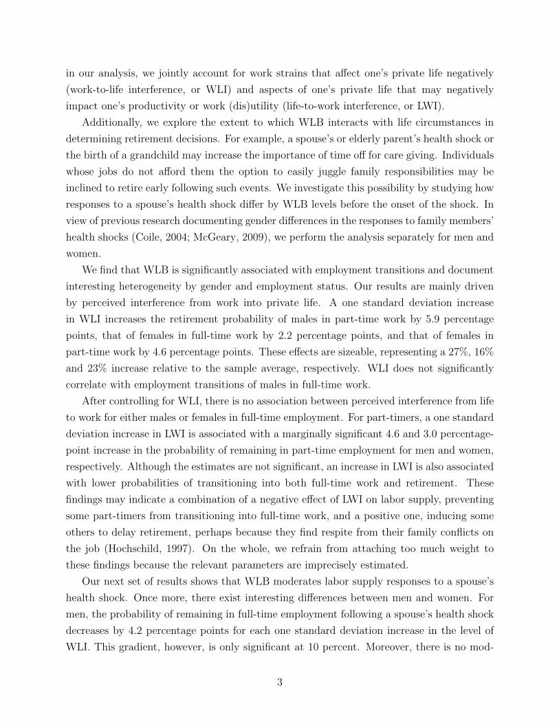
in our analysis, we jointly account for work strains that affect one’s private life negatively
(work-to-life interference, or WLI) and aspects of one’s private life that may negatively
impact one’s productivity or work (dis)utility (life-to-work interference, or LWI).
Additionally, we explore the extent to which WLB interacts with life circumstances in
determining retirement decisions. For example, a spouse’s or elderly parent’s health shock or
the birth of a grandchild may increase the importance of time off for care giving. Individuals
whose jobs do not afford them the option to easily juggle family responsibilities may be
inclined to retire early following such events. We investigate this possibility by studying how
responses to a spouse’s health shock differ by WLB levels before the onset of the shock. In
view of previous research documenting gender differences in the responses to family members’
health shocks (Coile, 2004; McGeary, 2009), we perform the analysis separately for men and
women.
We find that WLB is significantly associated with employment transitions and document
interesting heterogeneity by gender and employment status. Our results are mainly driven
by perceived interference from work into private life. A one standard deviation increase
in WLI increases the retirement probability of males in part-time work by 5.9 percentage
points, that of females in full-time work by 2.2 percentage points, and that of females in
part-time work by 4.6 percentage points. These effects are sizeable, representing a 27%, 16%
and 23% increase relative to the sample average, respectively. WLI does not significantly
correlate with employment transitions of males in full-time work.
After controlling for WLI, there is no association between perceived interference from life
to work for either males or females in full-time employment. For part-timers, a one standard
deviation increase in LWI is associated with a marginally significant 4.6 and 3.0 percentage-
point increase in the probability of remaining in part-time employment for men and women,
respectively. Although the estimates are not significant, an increase in LWI is also associated
with lower probabilities of transitioning into both full-time work and retirement. These
findings may indicate a combination of a negative effect of LWI on labor supply, preventing
some part-timers from transitioning into full-time work, and a positive one, inducing some
others to delay retirement, perhaps because they find respite from their family conflicts on
the job (Hochschild, 1997). On the whole, we refrain from attaching too much weight to
these findings because the relevant parameters are imprecisely estimated.
Our next set of results shows that WLB moderates labor supply responses to a spouse’s
health shock. Once more, there exist interesting differences between men and women. For
men, the probability of remaining in full-time employment following a spouse’s health shock
decreases by 4.2 percentage points for each one standard deviation increase in the level of
WLI. This gradient, however, is only significant at 10 percent. Moreover, there is no mod-
3

erating effect of WLI for part-timers. In line with previous studies (Coile, 2004; McGeary,
2009), women’s labor supply is more responsive to changes in spouses’ health, and those re-
sponses are moderated by the perceived degree of WLB. For women in full-time employment,
the probability of switching to a part-time job following a spouse’s health shock increases by
4 percentage points with each one standard deviation increase in WLI. For those employed
part-time, the probability of retirement is 8 percentage points higher for each one standard
deviation increase in the WLI index.
Our study is the first to address and quantify the association between WLB and actual
employment transitions of middle-age and older workers. Previous research has suggested
a potential link between WLB and retirement behavior by showing that full-time workers
in their early 50s who experience low levels of WLB are more likely to report a preference
for retiring within the next 10 years (Raymo and Sweeney, 2006). Interestingly, Raymo
and Sweeney find no gender differences in the association between WLB and self-reported
retirement intentions, while our paper shows that lack of WLB is more likely to induce
females than males to actually reduce their hours of work or withdraw from the labor force.
A further contribution of our study is to establish that life circumstances affect an individual’s
willingness to tolerate the absence of WLB, as hypothesized by Guest (2002). Specifically,
WLB moderates labor supply responses to spousal health shock.
The remaining of the paper proceeds as follows. Section 2 introduces the data and the
measures of WLB used in the analysis. Section 3 describes the empirical methodology and
presents the results. Section 4 concludes.
2 Data and Descriptive Statistics
We use data from the Health and Retirement Study (HRS), a multipurpose, longitudinal
household survey representing the U.S. population over the age of 50. Since 1992, the HRS
has surveyed age-eligible respondents and their spouses every two years to track transitions
from work into retirement, to measure economic well-being in later life and to monitor
changes in health status as individuals age. Initially, the HRS consisted of individuals born
between 1931 and 1941 and their spouses, but additional cohorts have been added in 1993,
1998, 2004, and 2010, the youngest representing individuals born between 1954 and 1959.
We primarily use data from the RAND version of the HRS, version P (Bugliari et al.,
2016). The RAND HRS is a large user-friendly subset of the HRS that combines data from
all waves, adds information that may have been provided by the spouse to the respondent’s
record and has consistent imputation of financial variables. We complement this data set
with additional variables from the employment module of each wave obtained from the
4

RAND FAT files. These are partially preprocessed files with all the raw HRS data of each
wave combined into a single respondent-level file.
In 2004, the HRS piloted a supplemental self-administered questionnaire that was left
with the respondent after the completion of an in-person core interview. This Leave-Behind
(LB) Questionnaire elicits respondents’ evaluations of their life circumstances, subjective
well-being, and lifestyle. Since 2004, the LB questionnaire has been administered in each
biennial wave to a (randomly selected) rotating 50% of the core sample who were assigned
to an in-person interview. This design implies that, for each respondent, LB measures are
available every other wave (or every four years). Importantly for our purpose, in 2006 a
number of questions about work-to-life and life-to-work interference were introduced in the
LB instrument (see below).
We include individuals aged 51 to 79 in our analysis sample, spanning the period 2006−2014. The HRS core questionnaire provides us with information about individual demo-
graphics and household characteristics, labor force status, pension arrangements, financial
situation, health status, and retirement expectations. We follow Maestas (2010) and An-
grisani et al. (2015) and classify individuals as full-time employees if they work at least 35
hours per week on their main job and as part-time employees if they work less than 35 hours
per week on their main job. We classify individuals as “retired” if they do not work for pay.
We exclude from the sample anyone who is self-employed, disabled, unemployed or out of
the labor force for reasons other than retirement according to the RAND HRS labor force
status definition.
The outcome of interest is the wave-to-wave transition between these labor force states.
We cannot consider transitions from complete retirement back to work, as work-life balance
measures are not available for retirees.1 There are 2, 448 male and 3, 011 female workers with
valid transitions for a total of 3, 036 and 3, 833 observations, respectively. Table 1 shows the
prevalence of labor force transitions aggregated across all waves by current employment
status and gender. The majority of full-time employees are still employed full-time in the
subsequent wave, with women more likely to transit into part-time than men. About 13% of
full-timers at time t are retired at time t+1. Among part-timers, male workers are relatively
more likely to move to full-time and to retire the next period, while female workers are more
likely to remain in part-time employment. Given this observed heterogeneity in labor supply
decisions, in what follows we will perform our analyses separately for full- and part-timers
as well as for men and women.
The HRS core questionnaire asks respondents who are currently working for pay about
1Maestas (2010) explicitly studies transitions from retirement to work, a phenomenon known as “unre-tirement”.
5

Table 1: Labor Force Transitions by Current Employment Status and Gender
Labor Force Status Labor Force Status at Time t+ 1: Totalat Time t Full-Time Part-Time Retirement
Male WorkersFull-Time 1,882 175 297 2,354
(79.95%) (7.43%) (12.62%) (100.00%)Part-Time 94 437 151 682
(13.78%) (64.08%) (22.14%) (100.00%)Total 1,976 612 448 3,036
(65.09%) (20.16%) (14.76%) (100.00%)
Female WorkersFull-Time 1,893 250 335 2,478
(76.39%) (10.09%) (13.52%) (100.00%)Part-Time 159 922 274 1,355
(11.73%) (68.04%) (20.22%) (100.00%)Total 2,052 1,172 609 3,833
(53.54%) (30.58%) (15.89%) (100.00%)
several aspects of their jobs. These include information about employer-provided pension
plans and health insurance, hourly wage, and nonmonetary characteristics. We will study
to what extent WLB influences employment transitions of older workers keeping monetary
incentives and other potential confounders constant. The richness of information available
in the HRS also allows us to control for the economic, health, and family circumstances that
are bound to affect labor supply decisions at older ages.
Table 2 presents descriptive statistics of the variables used in the analysis. Men are
slightly older than women. Among male workers, full-timers are about 6 years younger than
part-timers, while this difference is 4 years for women. Our sample covers a broad range of
educational backgrounds and other demographic characteristics. The proportion of men in
a couple household is above 80%, while it is about 65% among women. Men whose spouse is
working are significantly more likely to be working full-time than part-time, whereas there
are no detectable differences among women. The proportion of individuals in poor health is
only marginally higher for part-timers, while full-timers tend to have higher word recall score,
especially among men. Conditional on working full-time or part-time, men work more hours
per week and are better paid than women. They are also economically better off as they
hold, on average, more wealth. Not surprisingly, employer-provided pension plans and health
insurance coverage are substantially more common among full-time than part-time workers.
About one quarter of full-timers have a defined-benefit pension plan, 40% have a defined-
contribution pension plan, and the remaining 35% have no pension. Employer-sponsored
6

Table 2: Differences between Full- and Part-Time Workers
Men WomenMean Mean Diff. Mean Mean Diff.FT PT p-val FT PT p-val
Age 59.17 65.43 0.00 58.25 62.24 0.00Less than High School 0.12 0.14 0.08 0.11 0.15 0.00
High School 0.25 0.23 0.30 0.27 0.30 0.05Some College 0.27 0.24 0.12 0.31 0.29 0.39
College and Above 0.36 0.39 0.25 0.31 0.25 0.00In a Couple 0.84 0.84 0.92 0.64 0.67 0.10
Spouse Working 0.58 0.44 0.00 0.44 0.44 0.83Poor Health 0.12 0.14 0.31 0.13 0.15 0.23
Word Recall Score 0.04 -0.15 0.00 0.02 -0.04 0.06Test of 7 Score 0.00 -0.01 0.69 0.02 -0.03 0.13
Hours of Work per Week 45.69 21.06 0.00 42.69 20.83 0.00Hourly Wage (ihs) 3.79 3.56 0.00 3.60 3.34 0.00
DB Pension 0.23 0.06 0.00 0.25 0.09 0.00DC Pension 0.38 0.15 0.00 0.41 0.16 0.00No Pension 0.39 0.79 0.00 0.34 0.74 0.00
Emp. Health Ins. 0.68 0.34 0.00 0.72 0.27 0.00Emp. Health Ins. Covers S 0.37 0.21 0.00 0.22 0.07 0.00
Total HH Wealth (ihs) 11.36 11.78 0.10 10.79 11.12 0.11Work-Life Interference 0.21 -0.72 0.00 0.33 -0.60 0.00Life-Work Interference 0.05 -0.17 0.00 0.11 -0.19 0.00
N 2,354 682 3,036 2,478 1,355 3,833
Work-Life and Life-Work Interference indexes, Word Recall and Test of 7 scores arestandardized. Hourly wage and total household wealth are transformed using an inversehyperbolic sine transformation (ihs).
health insurance is marginally more prevalent among full-time women than men.
2.1 Measuring work-life balance
WLB can be loosely defined as the availability of “sufficient time to meet commitments both
at home and at work” (Guest, 2002). Because of the difficulty of measuring WLB directly,
in the paper we follow the existing literature on this topic and focus on its absence, that is,
instances of interference between work and life outside of work.
The conflict between work and life is bi-directional. Work-to-life interference (WLI) de-
scribes situations where the demands from work (e.g., long working hours, inflexible sched-
ules, expectations of constant availability, etc.) interfere with life outside of work. For
7

example, the need to work overtime may prevent a worker from accompanying their sick
spouse to a doctor’s appointment. Life-to-work interference (LWI) arises when non-work
burdens—such as the needs of adult children, caregiving to elderly parents and sick spouses,
or strained spousal relationships—spillover into work life. Along these lines, an individual’s
productivity on the job may decline while they provide care for their elderly mother. We
consider both dimensions separately in our analysis.
It has been proposed that WLB can be measured by both objective indicators, such as
the number of hours worked, and subjective indicators, such as individuals’ self-reports of the
degree of conflict between their work and family lives (Guest, 2002). In practice, though, it is
difficult to produce objective indicators of WLI or LWI without relying on strong assumptions
about what constitutes work-life balance. For instance, using an indicator of working long
hours as a proxy for WLI reflects an assumption that all workers assign a relatively similar
weight to work and home life, even though there is plenty of evidence that some workers
derive great satisfaction from working 60-hour weeks, and would not perceive this as an
intrusion into their family life (Peiperl and Jones, 2001).
Raymo and Sweeney (2006) provide further evidence of the limitations of objective mea-
sures of WLB. They show that controlling for potentially stressful job and family charac-
teristics (e.g., working long hours, working under continuous time pressure, having provided
care to a relative or friend in the last year, or having a spouse in poor health) has no effect
on the association between WLI, LWI and workers’ desire to transit into part-time work
or retirement. They conclude that objective measures of potentially stressing environments
cannot be taken as evidence of WLI or LWI unless they are actually perceived as stressful
by the worker.
The measures of WLI and LWI used in this paper are based on answers to a series
of questions eliciting the perceived conflict between an individual’s work and personal life.
These questions are listed in Table 3. Answers are given on the following four-point scale:
1 =rarely, 2 =sometimes, 3 =often, and 4 =most of the time. We reverse-code questions
LB048G-L, so that higher values indicate more interference between work and life for all
variables.
We create two indexes measuring WLI and LWI as the (standardized) first principal
component of the subset of variables that reflect each concept. For WLI, these are LB048A,
LB048B, LB048C, LB048G, LB048H, and LB048I; for LWI, these are LB048D, LB048E,
LB048F, LB048J, LB048K, and LB048L. As mentioned above, we can only measure WLB
every other wave for each respondent, because of the rotational design of the LB question-
naire.
As shown in Table 2, there are significant differences in the degree of perceived work-
8

Table 3: Work-Life Balance Measures Elicited by the LB Questionnaire
Question No. Question Text
LB048A My work schedule makes it difficult to fulfill personal responsibilitiesLB048B Because of my job, I don’t have the energy to do things with my family
or other important people in my lifeLB048C Job worries or problems distract me when I am not at workLB048D My home life keeps me from getting work done on time on my jobLB048E My family or personal life drains me of the energy I need to do my jobLB048F I am preoccupied with personal responsibilities while I am at workLB048G My work leaves me enough time to attend to my personal responsibilitiesLB048H My work gives me energy to do things with my family and other
important people in my lifeLB048I Because of my job, I am in a better mood at homeLB048J My personal responsibilities leave me enough time to do my jobLB048K My family or personal life gives me energy to do my jobLB048L I am in a better mood at work because of my family or personal life
life conflicts between full-timers and part-timers, with the former reporting higher levels of
interference. Among individuals working full-time, women report worse WLI and LWI than
men, with differences significant at the 1% level. Among part-timers, gender differences are
less pronounced and not statistically significant. In Table 4, we compare individuals with low
and high WLB. For this purpose, we construct a combined index of work-life interference
using both WLI and LWI measures and assign respondents to two groups depending on
whether their index is below (low work-life interference) or above (high work-life interference)
the sample median. Individuals with high interference tend to be a little younger and more
likely to be in poor health than those reporting low interference, while there are no significant
different as far as marital status, education and cognition are concerned. High work-life
interference is associated with more hours of work, but with better economic conditions,
especially among women. Female workers reporting relatively higher levels of conflict have
higher wages, are more likely to be enrolled in a pension plan, and are more likely to have
employer-sponsored health insurance. Individuals with high interference have significantly
less wealth, which, while suggesting worse retirement preparedness, may be also related to
their younger ages.
2.2 Measuring a Spouse’s Health Shocks
After establishing the effect of work-life balance and employment transitions in Section 3.1,
we assess, in Section 3.2, to what extent this relationship is moderated by changes in family
circumstances across two consecutive periods as represented by a spouse’s health shock.
9

Table 4: Differences between Workers with Low and High Work-Life Interference
Men WomenMean Mean Diff. Mean Mean Diff.Low High p-val Low High p-val
Age 61.75 59.40 0.00 60.75 58.57 0.00Less than High School 0.12 0.13 0.62 0.12 0.14 0.21
High School 0.24 0.24 0.70 0.29 0.27 0.10Some College 0.26 0.27 0.77 0.30 0.30 0.99
College and Above 0.38 0.36 0.35 0.28 0.29 0.49In a Couple 0.85 0.83 0.06 0.65 0.66 0.80
Spouse Working 0.55 0.55 1.00 0.44 0.45 0.59Poor Health 0.09 0.17 0.00 0.09 0.18 0.00
Word Recall Score 0.02 -0.02 0.35 0.01 -0.01 0.44Test of 7 Score 0.03 -0.03 0.11 0.02 -0.02 0.17
Hours of Work per Week 37.39 42.92 0.00 32.02 37.91 0.00Hourly Wage (ihs) 3.79 3.69 0.00 3.48 3.53 0.02
DB Pension 0.19 0.19 0.64 0.18 0.21 0.03DC Pension 0.31 0.35 0.05 0.29 0.35 0.00No Pension 0.50 0.46 0.03 0.53 0.44 0.00
Emp. Health Ins. 0.58 0.63 0.01 0.51 0.60 0.00Emp. Health Ins. Covers S 0.32 0.34 0.16 0.15 0.18 0.00
Total HH Wealth (ihs) 12.07 10.83 0.00 11.23 10.58 0.00N 1,518 1,518 3,036 1,917 1,916 3,833
We construct a combined index of Work-Life Interference by principal component analysisusing work-to-life interference and life-to-work interference measures. Low: below medianinterference; High: above median interference. Word Recall and Test of 7 scores arestandardized. Hourly wage and total household wealth are transformed using an inversehyperbolic sine transformation (ihs).
To this end, we follow McClellan (1998), Coile (2004), and Smith (2005) and construct
two indicator variables, one for the incidence of acute health issues between time t and
t + 1, including heart problems, strokes, and cancer, and one for new diagnoses of chronic
conditions such as diabetes, lung disease, high blood pressure, arthritis, and psychological
problems.2 In our sample, only about 5% of workers have a spouse who suffers an acute
health event, and 12.5% have a spouse who is newly diagnosed with a chronic condition
across to consecutive periods. In order to prevent cell sizes from becoming too small when
carrying out the analysis using the acute shock indicator separately by current employment
status and gender, we consider a spouse experiencing a health shock if the individual either
suffers an acute event or is newly diagnosed with a chronic condition.
2Our results do not change when we exclude psychological problems from this definition.
10

For the analysis investigating the interaction between WLB and spousal health shocks
in determining labor force transitions, we restrict the sample to couple households. After
excluding respondents for whom spousal health information is missing, we are left with
2, 443 male workers (1, 889 employed full-time and 554 employed part-time at baseline) and
2, 350 female workers (1, 496 in full-time employment and 854 in part-time employment at
baseline).
3 Empirical Analysis and Results
A number of factors shape labor supply decisions at older ages, from compensation, pension
arrangements and health insurance coverage, to family circumstances, work capability and
job demands. Likely, these factors indirectly impact WLB and interact with it to determine
the timing of and path to retirement. In our empirical analysis, we take advantage of
detailed information about older workers available in the HRS and estimate the effect of
WLB on labor supply decisions above and beyond the effect of other potential determinants.
Specifically, in our regressions, we account for age, education and marital status, for whether
the spouse is working and for spouse’s health status. We proxy individual ability to work
with self-reported health status and cognitive test scores. We then control for hours worked
per week, hourly wage, existence and type of employer-sponsored pension plan, employer-
provided health insurance policy and whether it covers the spouse. Finally, we add dummies
for total household wealth quartiles, to capture available resources to finance retirement, and
time fixed-effects to net out trends in retirement behavior over the observation period.
We estimate multinomial discrete choice models for the transitions from full-time employ-
ment into part-time and retirement and for the transitions from part-time employment into
full-time and retirement across two periods. This allows us to study a variety of retirement
paths that have been observed among older American workers in recent years (Chan and
Stevens, 2009). Moreover, recognizing the existence of potential gender differences in the
preference for work versus leisure/household activities as well as in the perception of how
work interferes with private life, we separately estimate our models for men and women.
Formally, we model the probability that a full-time or part-time worker observed at time
t transits to a different labor force status at time t+ 1 as:
P kij,t+1 = Pr (Yi,t+1 = j|Xi,t,WLBi,t, Yi,t = k) = F k
j
(Xi,t,WLBi,t, Yi,t = k; θkj
), (1)
where Yi,t+1 is the labor force status at time t+1, j = 1 (full-time), 2 (part-time), 3 (retired),
Xi,t is a vector of explanatory variables observed at time t, WLBi,t contains the two indexes
11

measuring WLI and LWI at time t (higher values of these indexes correspond to worse WLB),
and the superscript k indicates labor force status at time t (either full-time, k = 1, or part-
time, k = 2). The function F kj is a probability function depending on a vector of unknown
parameters θkj . We adopt a Multinomial Logit model, hence:
F kj
(Xi,t,WLBi,t, Yi,t = k; θkj
)=
exp(V kij
)∑3l=1 exp
(V kil
) , j = 1, 2, 3, (2)
where
V kij = X ′
i,tαkj +WLB′
i,tβkj (3)
and θkj ≡(αkj β
kj
)′. To ease the notation, we omit a superscript for male and female workers.
Nonetheless, all model parameters are considered gender-specific and separately estimated
for men and women.
We denote the marginal effect of a variable Z on choice j for individual i in period t with:
MEijZ,t
(θkj)
=∂F k
j
(Xi,t,WLBi,t, Yi,t = k; θkj
)∂Zi,t
. (4)
We estimate and report in the tables below the average marginal effects, that is:
M̄EijZ,t
(θ̂kj
)=
1
N
N∑i=1
1
Ti
4∑t=1
Di,tMEijZ,t
(θ̂kj
), (5)
where N is the number of individuals in our sample, Ti is the number of transitions in our
sample for individual i and Di,t is equal to 1, if the transition between waves t and t+ 1 of
individual i is in our sample, and to 0 otherwise. Standard errors are computed by the delta
method and clustered at the individual level, since the same individual i may be represented
in multiple observations (from different waves).
3.1 Regressions by Employment Status at Time t and Gender
WLB and employment transitions of male workers
Table 5 shows the estimated marginal effects for male workers. For men working full-
time at time t, WLI is associated with a lower likelihood of remaining in full-time and a
correspondingly greater probability of retirement at time t+ 1, although the coefficients are
not statistically significant. The association is stronger for individuals employed part-time
at time t: a one standard deviation increase in the WLI index decreases the likelihood of
remaining part-time employed at time t + 1 by 7 percentage points, while increasing the
12
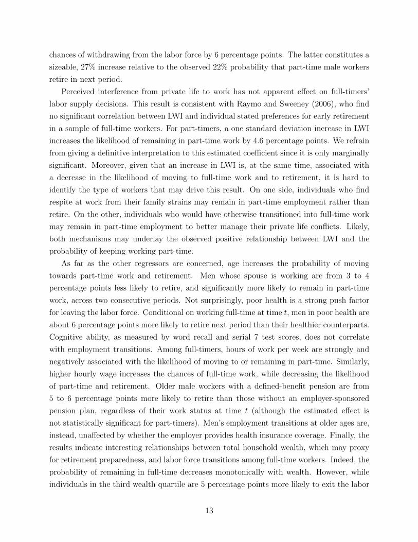
chances of withdrawing from the labor force by 6 percentage points. The latter constitutes a
sizeable, 27% increase relative to the observed 22% probability that part-time male workers
retire in next period.
Perceived interference from private life to work has not apparent effect on full-timers’
labor supply decisions. This result is consistent with Raymo and Sweeney (2006), who find
no significant correlation between LWI and individual stated preferences for early retirement
in a sample of full-time workers. For part-timers, a one standard deviation increase in LWI
increases the likelihood of remaining in part-time work by 4.6 percentage points. We refrain
from giving a definitive interpretation to this estimated coefficient since it is only marginally
significant. Moreover, given that an increase in LWI is, at the same time, associated with
a decrease in the likelihood of moving to full-time work and to retirement, it is hard to
identify the type of workers that may drive this result. On one side, individuals who find
respite at work from their family strains may remain in part-time employment rather than
retire. On the other, individuals who would have otherwise transitioned into full-time work
may remain in part-time employment to better manage their private life conflicts. Likely,
both mechanisms may underlay the observed positive relationship between LWI and the
probability of keeping working part-time.
As far as the other regressors are concerned, age increases the probability of moving
towards part-time work and retirement. Men whose spouse is working are from 3 to 4
percentage points less likely to retire, and significantly more likely to remain in part-time
work, across two consecutive periods. Not surprisingly, poor health is a strong push factor
for leaving the labor force. Conditional on working full-time at time t, men in poor health are
about 6 percentage points more likely to retire next period than their healthier counterparts.
Cognitive ability, as measured by word recall and serial 7 test scores, does not correlate
with employment transitions. Among full-timers, hours of work per week are strongly and
negatively associated with the likelihood of moving to or remaining in part-time. Similarly,
higher hourly wage increases the chances of full-time work, while decreasing the likelihood
of part-time and retirement. Older male workers with a defined-benefit pension are from
5 to 6 percentage points more likely to retire than those without an employer-sponsored
pension plan, regardless of their work status at time t (although the estimated effect is
not statistically significant for part-timers). Men’s employment transitions at older ages are,
instead, unaffected by whether the employer provides health insurance coverage. Finally, the
results indicate interesting relationships between total household wealth, which may proxy
for retirement preparedness, and labor force transitions among full-time workers. Indeed, the
probability of remaining in full-time decreases monotonically with wealth. However, while
individuals in the third wealth quartile are 5 percentage points more likely to exit the labor
13
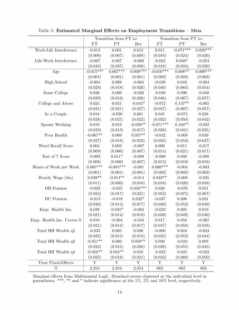
Table 5: Estimated Marginal Effects on Employment Transitions – Men
Transition from FT to: Transition from PT to:FT PT Ret FT PT Ret
Work-Life Interference -0.013 0.001 0.012 0.011 -0.071*** 0.059***(0.009) (0.007) (0.008) (0.016) (0.024) (0.020)
Life-Work Interference -0.007 0.007 -0.000 -0.022 0.046* -0.024(0.010) (0.007) (0.008) (0.018) (0.024) (0.020)
Age -0.015*** 0.007*** 0.009*** -0.016*** 0.008** 0.009***(0.001) (0.001) (0.001) (0.002) (0.003) (0.003)
High School -0.004 0.008 -0.004 -0.039 0.043 -0.004(0.029) (0.018) (0.026) (0.046) (0.064) (0.054)
Some College 0.026 0.000 -0.026 -0.049 0.096 -0.048(0.029) (0.018) (0.026) (0.046) (0.067) (0.057)
College and Above 0.024 0.021 -0.045* -0.072 0.137** -0.065(0.031) (0.021) (0.027) (0.047) (0.067) (0.057)
In a Couple 0.018 -0.020 0.001 0.045 -0.074 0.028(0.028) (0.021) (0.022) (0.032) (0.050) (0.042)
Spouse Working 0.019 0.019 -0.038** -0.071*** 0.104** -0.032(0.019) (0.013) (0.017) (0.026) (0.041) (0.035)
Poor Health -0.067** 0.009 0.057** -0.042 -0.008 0.049(0.027) (0.018) (0.023) (0.033) (0.053) (0.047)
Word Recall Score 0.004 0.003 -0.007 0.006 0.011 -0.017(0.009) (0.006) (0.007) (0.014) (0.021) (0.017)
Test of 7 Score -0.003 0.011* -0.008 -0.000 0.008 -0.008(0.008) (0.006) (0.007) (0.013) (0.019) (0.016)
Hours of Work per Week 0.005*** -0.004*** -0.001 0.006*** -0.004 -0.003(0.001) (0.001) (0.001) (0.002) (0.002) (0.002)
Hourly Wage (ihs) 0.029** -0.014** -0.014 0.033** -0.008 -0.025(0.011) (0.006) (0.010) (0.016) (0.020) (0.016)
DB Pension -0.033 -0.025 0.058*** 0.026 -0.076 0.051(0.024) (0.017) (0.021) (0.053) (0.075) (0.067)
DC Pension -0.013 -0.019 0.032* -0.037 0.006 0.031(0.020) (0.014) (0.017) (0.030) (0.052) (0.049)
Emp. Health Ins. 0.029 -0.025* -0.004 -0.023 0.005 0.019(0.021) (0.014) (0.018) (0.039) (0.049) (0.040)
Emp. Health Ins. Covers S 0.019 -0.004 -0.016 0.017 0.050 -0.067(0.021) (0.014) (0.017) (0.047) (0.058) (0.043)
Total HH Wealth q2 -0.035 0.005 0.030 -0.000 0.024 -0.024(0.022) (0.015) (0.018) (0.035) (0.052) (0.044)
Total HH Wealth q3 -0.051** 0.000 0.050** 0.030 -0.034 0.003(0.023) (0.015) (0.020) (0.038) (0.055) (0.045)
Total HH Wealth q4 -0.058** 0.042** 0.016 -0.023 0.045 -0.022(0.025) (0.018) (0.021) (0.042) (0.060) (0.050)
Time Fixed-Effects Y Y Y Y Y Y
N 2,354 2,354 2,354 682 682 682
Marginal effects from Multinomial Logit. Standard errors clustered at the individual level inparentheses. ***, ** and * indicate significance at the 1%, 5% and 10% level, respectively.
14

force altogether, those in the fourth wealth quartile are more likely to move to part-time.
WLB and employment transitions of female workers
Estimates for women are reported in Table 6. In general, increases in WLI push women
towards retirement. Specifically, for full-timers a one standard deviation increase in WLI
increases the chances of retirement by 2.2 percentage points, a 16% increase from the 14%
sample average. The effect is more sizeable for part-timers. For them, a one standard devia-
tion increase in WLI leads to a 4.6 percentage-point increase in the likelihood of retirement.
This represents a 23% increase from the 20% sample average. As was the case for male work-
ers, there is no association between LWI and labor force transitions for full-timers and only
a weak correlation between LWI and the probability that part-timers ramain in part-time
employment.
The effect of age on female workers’ transition probabilities is similar to the one observed
for men: one more year of age increases the likelihood of retirement by about 1.5 and 1
percentage points among full-timers and part-timers, respectively. Women’s labor supply
decisions appear to be less influenced by whether or not the spouse is currently working
among full-timers than part-timers. Being in poor health makes women working full-time
4.8 percentage points less likely to remain in full-time, 3.2 percentage points less likely to
move to part-time, and 8.1 percentage points more likely to retire. In contrast, health does
not correlate with employment transitions of women working part-time at time t. Also among
women, full-timers working more hours per week tend to remain in full-time employment and
are less likely to switch to part-time. For those already in part-time at time t, one more hour
of work per week is associated with a greater probability of moving to full-time and lower
chances of retirement. These patterns may reflect strong preferences for work over leisure for
some individuals. Women respond somewhat more decisively to pension incentives than men.
Among full-timers, individuals with a defined-benefit pension plan are 8.4 percentage points
less likely to move to part-time and about 7 percentage points more likely to retire than
those with no pension, while individuals with a defined-contribution plan are 3.5 percentage
points more likely to remain in full-time and 5.7 percentage points less likely to switch to
part-time. Pension arrangements are not associated with labor force transitions among part-
time female workers. Employer-provided health insurance is a critical pull factor for women.
Being covered by an employer’s health plan increases the probability of remaining in full-
time by 8.5 percentage points and decreases the chances of working part-time or retiring by
5.7 and 2.7 percentage points, respectively (although the latter coefficient is not statistically
significant). There is also suggestive evidence that female workers whose spouse is covered by
their employer’s health plan avoid changing their employment status across two consecutive
periods. Finally, for women working part-time at time t, more household wealth is associated
15

Table 6: Estimated Marginal Effects on Employment Transitions – Women
Transition from FT to: Transition from PT to:FT PT Ret FT PT Ret
Work-Life Interference -0.020** -0.002 0.022*** 0.003 -0.049*** 0.046***(0.010) (0.007) (0.008) (0.010) (0.016) (0.014)
Life-Work Interference -0.009 0.008 0.001 -0.014 0.030* -0.016(0.010) (0.006) (0.008) (0.010) (0.016) (0.014)
Age -0.017*** 0.004*** 0.013*** -0.009*** 0.000 0.009***(0.002) (0.001) (0.001) (0.002) (0.002) (0.001)
High School -0.000 0.006 -0.005 -0.006 0.043 -0.036(0.029) (0.018) (0.025) (0.028) (0.042) (0.034)
Some College 0.021 0.014 -0.035 -0.024 0.044 -0.020(0.029) (0.018) (0.025) (0.029) (0.044) (0.037)
College and Above 0.036 0.024 -0.060** 0.023 0.023 -0.045(0.033) (0.022) (0.027) (0.032) (0.049) (0.041)
In a Couple 0.007 -0.006 -0.002 0.023 -0.053 0.029(0.024) (0.018) (0.019) (0.023) (0.034) (0.027)
Spouse Working -0.005 -0.002 0.007 -0.053** 0.068* -0.015(0.023) (0.017) (0.018) (0.023) (0.035) (0.029)
Poor Health -0.048* -0.032** 0.081*** -0.029 0.023 0.006(0.025) (0.016) (0.022) (0.024) (0.037) (0.031)
Word Recall Score 0.007 -0.000 -0.007 0.002 0.003 -0.005(0.008) (0.006) (0.007) (0.010) (0.015) (0.012)
Test of 7 Score -0.014 0.007 0.007 0.001 0.009 -0.010(0.009) (0.007) (0.007) (0.009) (0.013) (0.011)
Hours of Work per Week 0.005*** -0.004*** -0.001 0.007*** -0.001 -0.006***(0.001) (0.001) (0.001) (0.001) (0.002) (0.001)
Hourly Wage (ihs) 0.020 -0.018* -0.002 0.013 0.007 -0.020(0.016) (0.010) (0.013) (0.015) (0.019) (0.015)
DB Pension 0.014 -0.084*** 0.069*** 0.005 -0.006 0.001(0.024) (0.017) (0.020) (0.029) (0.046) (0.040)
DC Pension 0.035* -0.057*** 0.022 0.011 -0.007 -0.004(0.021) (0.016) (0.016) (0.023) (0.037) (0.032)
Emp. Health Ins. 0.085*** -0.057*** -0.027 -0.011 -0.013 0.024(0.022) (0.017) (0.018) (0.022) (0.034) (0.030)
Emp. Health Ins. Covers S 0.037 -0.032* -0.005 0.014 0.072 -0.086**(0.023) (0.017) (0.019) (0.036) (0.055) (0.042)
Total HH Wealth q2 0.028 -0.023 -0.005 -0.022 0.003 0.019(0.023) (0.016) (0.018) (0.028) (0.038) (0.031)
Total HH Wealth q3 0.024 -0.024 -0.000 -0.030 0.037 -0.007(0.024) (0.017) (0.020) (0.029) (0.041) (0.033)
Total HH Wealth q4 -0.027 0.016 0.011 -0.058** 0.102** -0.044(0.027) (0.020) (0.022) (0.029) (0.043) (0.036)
Time Fixed-Effects Y Y Y Y Y Y
N 2,478 2,478 2,478 1,355 1,355 1,355
Marginal effects from Multinomial Logit. Standard errors clustered at the individual level inparentheses. ***, ** and * indicate significance at the 1%, 5% and 10% level, respectively.
16

with a higher probability of remaining in part-time and, conversely, with lower chances of
transitioning to full-time employment or retirement.
3.2 Interaction between WLB and Changes in Spouse’s Health
The effect of WLB on employment transitions may vary with life circumstances. For instance,
a spouse’s or elderly parent’s health shock may increase the importance of time off for
care giving. Individuals whose jobs do not afford them the option to easily juggle family
responsibilities may be inclined to reduce their hours of work or exit the labor force following
such events. We investigate this hypothesis focusing on the WLI index, which, as shown
above, correlates most strongly with labor force transitions, and by interacting it with the
onset of a spouse’s health shock across two consecutive periods. More precisely, we specify
the Multinomial Logit single index function as follows:
V kij = X ′
i,tαkj +WLIi,tβ
kj + SpHSi,tγ
kj + (WLIi,t × SpHSi,t) δ
kj , (6)
where, again, the superscript k indicates employment status at time t (either full-time, k = 1,
or part-time, k = 2) and model’s parameters are treated as gender-specific. The variable
SpHSi,t, defined in the data section, captures the onset of a spouse’s acute health issue or
newly diagnosed chronic condition.
We estimate the marginal effects of a spouse’s health shock on employment transitions
at different levels of WLI. Figures 1-4 show the point estimates and the corresponding 95%
confidence intervals by gender and employment status at time t. This analysis is comple-
mented with regressions of the individual-level marginal effects of a spouse’s health shock
on the WLI index. The estimated coefficients from these regressions can be interpreted as
summary statistics of the extent to which poor WLB interacts with a spouse’s health shock
to shape retirement paths (i.e., how the likelihood of partially or fully retiring following a
spouse’s health shock varies with increases in the level of perceived WLI). We adopt a boot-
strap procedure (with 500 replications) to compute the standard error of these parameters.
This accounts for the estimation error of the first-step Multinomial Logit marginal effects,
which are then used as dependent variables in the second-step regressions.
Figure 1 shows that, for male workers employed full-time, the likelihood of remaining in
full-time employment following a spouse’s health shock decreases as WLI increases. While
a spouse’s health shock has no effect on the probability of remaining in full-time work
for individuals with the lowest WLI, it is associated with an 18 percentage-point decline
(significant at 10%) for those with the highest WLI. In Table 7, we estimate that, following
a spouse’s health shock, the probability that men remain in full-time employment decreases
17

Figure 1: Male Workers in Full-Time at Time tEffect of a Spouse’s Health Shock on:
-.4-.3
-.2-.1
0.1
Lowest HighestWLI
Pr(Full-Time at Time t+1)
-.10
.1.2
.3
Lowest HighestWLI
Pr(Part-Time at Time t+1)
-.10
.1.2
Lowest HighestWLI
Pr(Retirement at Time t+1)
Figure 2: Male Workers in Part-Time at Time tEffect of a Spouse’s Health Shock on:
-.50
.51
Lowest HighestWLI
Pr(Full-Time at Time t+1)
-.6-.4
-.20
.2
Lowest HighestWLI
Pr(Part-Time at Time t+1)
-1-.5
0.5
1
Lowest HighestWLI
Pr(Retirement at Time t+1)
18

Figure 3: Female Workers in Full-Time at Time tEffect of a Spouse’s Health Shock on:
-.3-.2
-.10
.1.2
Lowest HighestWLI
Pr(Full-Time at Time t+1)
-.10
.1.2
.3
Lowest HighestWLI
Pr(Part-Time at Time t+1)
-.2-.1
0.1
.2
Lowest HighestWLI
Pr(Retirement at Time t+1)
Figure 4: Female Workers in Part-Time at Time tEffect of a Spouse’s Health Shock on:
-.2-.1
0.1
.2
Lowest HighestWLI
Pr(Full-Time at Time t+1)
-.8-.6
-.4-.2
0.2
Lowest HighestWLI
Pr(Part-Time at Time t+1)
-.20
.2.4
.6.8
Lowest HighestWLI
Pr(Retirement at Time t+1)
19

by 4.2 percentage points for each one standard deviation increase in the level of work-to-life
interference. Figure 2 shows that men working part-time at time t respond relatively little
the the onset of spousal health issues. Moreover, this response does not vary with the degree
of WLI.
In line with previous studies (Coile, 2004; McGeary, 2009), female workers tend to de-
crease their labor supply more in response to a spouse’s health shock than their male counter-
parts. Most importantly, these responses depend on the perceived degree of WLB. Figure 3
shows a very clear WLI-gradient in the effect of a spouse’s health shock on labor force transi-
tions of women in full-time work. At low levels of WLI, a spouse’s health shock is associated
with a 7 percentage-point increase in the likelihood of remaining in full-time employment
and, conversely, with a 5 percentage-point decrease in the probability of transitioning to
part-time employment. As the degree of WLI increases, full-time female workers exhibit a
marked tendency to move to part-time after a spouse’s health shock. In general, following
a spouse’s health shock, the probability that women working full-time at time t switch to
part-time at time t + 1 increases by 4 percentage points for each one standard deviation
increase in the WLI index. There is, instead, no evidence of direct transitions from full-time
to retirement after the onset of a spouse’s health issues.
Table 7: Regression of Spouse’s Health Shock Marginal Effect on WLI(Estimated Coefficient)
Transition to:FT PT Ret
Men, Full-Time -0.042* 0.026 0.016(N = 1, 889) (0.024) (0.020) (0.018)
Men, Part-Time 0.045 -0.057 0.013(N = 554) (0.053) (0.064) (0.048)
Women, Full-Time -0.041 0.040** 0.001(N = 1, 496) (0.027) (0.020) (0.022)
Women, Part-Time 0.016 -0.097** 0.080**(N = 854) (0.031) (0.049) (0.040)
Bootstrap standard errors (500 replications) clustered at the individuallevel in parentheses. ***, ** and * indicate significance at the 1%, 5% and10% level, respectively.
As shown in Figure 4, women working part-time are more likely to respond to a spouse’s
health shock by withdrawing from the labor force. Again, this response is rather heteroge-
neous, depending on the current work-life balance situation. At the lowest level of work-to-life
conflict, female part-timers are 10 points more likely to stay in part-time and 7 percentage
points less likely to retire if the spouse developed new acute or chronic conditions. In con-
20

trast, those facing the highest degree of WLI are about 35 percentage points less likely to
keep working in the following period and about 35 percentage points more likely to retire.
Table 7 indicates that, for women working part-time, a spouse’s health shock decreases the
probability of remaining in part-time by over 9 percentage points, and increases the likeli-
hood of retirement by 8 percentage points, for each one standard deviation increase in the
WLI index.
4 Conclusions
Work-life balance (WLB) is likely an important determinant of employment decisions. There
is ample anecdotal evidence suggesting that workers who perceive that their jobs are an ob-
stacle to the successful management of their private life are less likely to remain employed.
For instance, in middle-age families where working individuals are responsible both for bring-
ing up their own children and for the care of their ageing parents, or in couples approaching
retirement age where one of the spouses suffers health problems, a good or bad WLB can
make the difference between continuing working or dropping out of the labor force. Yet, the
extent to which the degree of perceived WLB influences labor supply decisions remains to
be established and quantified. In this paper, we take on this task and study the relation
between WLB and employment transitions among middle-age and older workers.
Changing retirement patterns over the last few decades mean that retirement can no
longer be thought of as a binary choice between full-time work and complete exit from the
labor force (Ruhm (1990), Cahill et al. (2015)). A common, alternative path is to move to a
part-time or bridge job before fully retiring. Partial retirement arrangements are particularly
important in the context of our research, as they may afford a better balance between
work and family responsibilities, while prolonging individuals’ attachment to the labor force.
To allow for the variety of retirement paths available to individual nowadays we estimate
multinomial discrete choice models for the transitions from full-time employment into part-
time and retirement and for the transitions from part-time employment into full-time and
retirement across two consecutive periods. Moreover, recognizing the existence of potential
gender differences in the preference for work versus leisure and household production, as
well as in the perception of how work interferes with private life, we separately estimate
our models for men and women. Hence, we provide an extensive analysis of employment
transitions at older ages and we document heterogeneity in the extent to which WLB might
affect these decisions.
The conflict between work and private life is potentially bi-directional (Frone et al. (1992),
Guest (2002)). In our analysis, we distinguish between work-to-life interference (WLI),
21

that is, instances were work demands affect individuals’ ability to manage their private life
satisfactorily; and life-to-work interference (LWI), which refers to private life responsibilities
that affect job performance and productivity.
We use data from the Health and Retirement Study (HRS), a longitudinal survey repre-
sentative of the U.S. population over the age of 50 which provides detailed information about
individuals’ and couples’ economic status, health, demographics, and job characteristics. In-
dividuals’ perceptions of WLI and LWI are elicited through the Leave-Behind Questionnaire,
which is administered to half of the panel in each biennial wave. The richness of the HRS
data allows us to study the effects of WLI and LWI on employment transitions jointly,
while controlling for a rich set of other determinants ranging from demographics, health and
household wealth to wage, pension plan enrollment and health insurance benefits.
We find that WLB is significantly associated with employment transitions. Such asso-
ciation is mainly driven by WLI, whereas LWI correlates only weakly with labor supply
decisions of older workers. Interestingly, there exists great heterogeneity in the response
to perceived WLB by gender and employment status at baseline. A one standard devia-
tion increase in WLI increases the retirement probability of males in part-time work by 5.9
percentage points, that of females in full-time work by 2.2 percentage points, and that of
females in part-time work by 4.6 percentage points. These effects are sizeable, representing
a 27%, 16% and 23% increase relative to the sample average, respectively. WLI does not
significantly correlate with employment transitions of males in full-time work.
A prime example of a situation in which WLB may tip the scales in favor of continued
employment or retirement is when an individual’s spouse experiences a health shock. This
may require new care giving responsibilities and also affect expectations about mortality,
which in itself may alter the relative utility of work versus leisure. We show that WLB
moderates labor supply responses to a spouse’s health shock and differentially so for men and
women. For men, the probability of remaining in full-time employment following a spouse’s
health shock decreases by 4.2 percentage points for each one standard deviation increase in
the level of WLI. This gradient, however, is only significant at 10 percent. Moreover, there
is no moderating effect of WLI for part-timers. For women in full-time employment, the
probability of switching to a part-time job following a spouse’s health shock increases by 4
percentage points with each one standard deviation increase in WLI. For those employed
part-time, the probability of retirement is 8 percentage points higher for each one standard
deviation increase in the WLI index.
A limitation of our study is that, while controlling for a wide array of variables that may
affect both WLB and employment transitions, we cannot completely rule out that other,
unobservable factors may drive the estimated relations between WLB and labor supply
22

decisions. Because of that, we have refrained from making causal claims throughout the text.
Such factors plausibly comprise individual aptitudes and preferences underlaying selection
into jobs with certain characteristics, including level of WLB, as well as tastes for mode
and timing of retirement. It should be noted, however, that these individual traits would
likely bias our parameters of interest downward, and hence towards the null hypothesis of no
relationship between WLB and employment transitions. We would expect individuals who
have a stronger preference for leisure over work to have a higher likelihood of selecting into
jobs with better WLB and to retire earlier, other things equal. This selection mechanism
would imply that individuals with better WLB would be more prone to reduce their labor
supply. Our findings that worse WLB is associated with a higher likelihood of transiting into
partial and full retirement contradict this argument, and are suggestive of a causal, positive
link between WLB and prolonged attachment to the labor force.
The institutional framework where individuals work is bound to affect experienced work-
life balance. Laws that make it mandatory for employers to facilitate part-time or paid
leave opportunities to help employees juggle family responsibilities may improve WLB and,
in turn, facilitate longer labor force attachment of older workers. Policy changes affecting
the work flexibility of some workers and not of others (e.g., paid family leave insurance
laws becoming effective in California, New Jersey, Rhode Island, and Washington between
2004 and 2019) may also be exploited to infer stronger and more robust causal relationships
between WLB and employment transitions.3 We leave this for future research.
References
Angrisani, M., M. D. Hurd, E. Meijer, A. M. Parker, and S. Rohwedder (2017). Person-
ality and employment transitions at older ages: Direct and indirect effects through non-
monetary job characteristics. Labour 31, 127–152.
Angrisani, M., A. Kapteyn, and E. Meijer (2015). Nonmonetary job characteristics and
employment transitions at older ages. Working Paper, University of Michigan Retirement
Research Center (WP 2015-326).
Bianchi, S. M. and M. A. Milkie (2010). Work and family research in the first decade of the
21st century. Journal of Marriage and Family 72, 705–725.
Bugliari, D. et al. (2016). RAND HRS Data Documentation, Version P. Santa Monica, CA:
RAND Corporation, Center for the Study of Aging.
3Rossin-Slater et al. (2013) evaluate the effect of the introduction of California’s Paid Family Leave lawon the labor supply of women of child-bearing age.
23
Cahill, K. E., M. D. Giandrea, and J. F. Quinn (2015). Retirement patterns and the macroe-
conomy, the prevalence and determinants of bridge jobs, phased retirement, and reentry
among three recent cohorts of older americans. Gerontologist 55, 384–403.
Chan, S. and A. H. Stevens (2009). Is retirement being remade? developments in labor mar-
ket patterns at older ages. In J. Ameriks and O. Mitchell (Eds.), Recalibrating Retirement
Spending and Saving. Oxford Scholarship Online.
Coile, C. C. (2004). Health shocks and couples’ labor supply decisions. NBER Working
Paper No. 10810 .
Currie, J. and B. C. Madrian (1999). Health, health insurance and the labor market. In
O. Ashenfelter and D. Card (Eds.), Handbook of Labor Economics, Volume 3, pp. 3309–
3407. Elsevier.
French, E. (2005). The effects of health, wealth, and wages on labour supply and retirement
behaviour. The Review of Economic Studies 72, 395–427.
French, E. and J. B. Jones (2011). The effects of health insurance and self-insurance on
retirement behavior. Econometrica 79, 693–732.
Frone, M. R., M. Russell, and M. L. Cooper (1992). Prevalence of work-family conflict:
Are work and family boundaries asymmetrically permeable? Journal of Organizational
Behavior 13, 723–729.
Gardiner, J., M. Stuart, C. Forde, I. Greenwood, R. MacKenzie, and R. Perrett (2007). Work
life balance and older workers: Employees’ perspectives on retirement transitions following
redundancy. International Journal of Human Resource Management 18, 476–489.
Gruber, J. and D. A. Wise (2004). Social Security Programs and Retirement around the
World: Micro-Estimation. Chicago, IL: University of Chicago Press.
Guest, D. E. (2002). Perspectives on the study of work-life balance. Social Science Infor-
mation 41, 255–279.
Hochschild, A. (1997). The time bind. WorkingUSA 1, 21–29.
Lewis, J. (2008). Work-family balance policies: Issues and development in the uk 1997-
2005 in comparative perspective. In J. Scott, S. Dex, and H. Joshi (Eds.), Women and
Employment: Changing Lives and New Challenges, pp. 268–288. Cheltenham, UK: Edward
Elgar.
24

Lumsdaine, R. L. and O. S. Mitchell (1999). New developments in the economic analysis
of retirement. In O. Ashenfelter and D. Card (Eds.), Handbook of Labor Economics,
Volume 3, pp. 3261–3307. Elsevier.
Maestas, N. (2010). Back to work: Expectations and realizations of work after retirement.
Journal of Human Resources 45, 718748.
McClellan, M. B. (1998). Health events, health insurance, and labor supply: evidence from
the health and retirement survey. In D. A. Wise (Ed.), Frontiers in the Economics of
Aging, pp. 301–350. University of Chicago Press.
McGeary, K. A. (2009). How do health shocks influence retirement decisions? Review of
Economics of the Household 7, 307–321.
Peiperl, M. and B. Jones (2001). Workaholics and overworkers: Productivity or pathology?
Group & Organization Management 26, 369–393.
Raymo, J. M. and M. M. Sweeney (2006). Work-family conflict and retirement preferences.
The Journals of Gerontology Series B: Psychological Sciences and Social Sciences 61,
S161–S169.
Rossin-Slater, M., C. J. Ruhm, and J. Waldfogel (2013). The effects of california’s paid
family leave program on mothers’ leave-taking and subsequent labor market outcomes.
Journal of Policy Analysis and Management 32, 224–245.
Ruhm, C. J. (1990). Bridge jobs and partial retirement. Journal of Labor Economics 8,
482–501.
Smith, J. P. (2005). Consequences and predictors of new health events. In D. A. Wise (Ed.),
Analyses in the Economics of Aging, pp. 213–237. University of Chicago Press.
Wise, D. A. (2010). Facilitating longer working lives: International evidence on why and
how. Demography 47, S131–S149.
25