women's emancipation through education: a macroeconomic
TRANSCRIPT

JID:YREDY AID:710 /FLA [m3G; v1.143-dev; Prn:17/12/2014; 13:01] P.1 (1-26)
Review of Economic Dynamics ••• (••••) •••–•••
Contents lists available at ScienceDirect
Review of Economic Dynamics
www.elsevier.com/locate/red
Women’s emancipation through education: A macroeconomic
analysis ✩
Fatih Guvenen a,b, Michelle Rendall c,∗
a University of Minnesota, United Statesb NBER, United Statesc University of Zurich, Switzerland
a r t i c l e i n f o a b s t r a c t
Article history:Received 25 June 2014Received in revised form 22 November 2014Available online xxxx
JEL classification:D13E24J12
Keywords:MarriageDivorceRemarriageCollege-gender gapFemale labor supplyDivorce law reform
We study the role of education as insurance against a bad marriage in light of changing divorce laws during the 1970s. We build and estimate an equilibrium search model with education, marriage/divorce/remarriage, and household labor supply decisions. A key feature of the model is that women bear a larger share of the divorce burden, mainly because they are more closely tied to their children relative to men. Our focus on education is motivated by the fact that divorce laws typically allow spouses to keep the future returns from their human capital upon divorce (unlike their physical assets), making education a good insurance in divorce. In the model, women overtake men in college attainment during the 1990s, a feature of the data that has proved challenging to explain. Our counterfactual experiments indicate that the divorce law reform of the 1970s played an important role in these trends, explaining more than one-quarter of college attainment rate of women post-1970s and one-half of the rise in labor supply for married women. Further, results suggest a higher insurance value of education in divorce than marriage market signaling benefits of education especially for women post divorce reform.
© 2014 Elsevier Inc. All rights reserved.
1. Introduction
In this paper, we study the role of education as insurance against a bad marriage. Historically, disparities in earning power and education across genders have contributed to creating a vulnerable economic position for married women. Women in bad marriages are faced with suffering one of two fates: either divorce (assuming it is available) and struggle as low-income single mothers, or remain trapped in the marriage. The following two examples are instructive.
First, writer Ilka Perez recounts her own experience as an uneducated divorced mother:
✩ We would like to thank seminar and conference participants at the European University Institute, Goethe University of Frankfurt, Toulouse School of Economics, Universite Catholique de Louvain, University of Konstanz, University College London, the Society for Economic Dynamics 2012 Meeting, the NBER Summer Institute 2012, Minnesota Workshop in Macroeconomic Theory 2013, ZEW Mannheim Family Workshop 2013, and the Overlapping Generations Days at the Paris School of Economics 2014 for valuable comments. For financial support, Guvenen thanks the National Science Foundation (Grant No. 0814030) and Rendall thanks the European Research Council (ERC Advanced Grant IPCDP-229883) and the ZUNIV FAN Research Talent Development Fund. The usual disclaimer applies.
* Corresponding author.E-mail addresses: [email protected] (F. Guvenen), [email protected] (M. Rendall).URLs: http://www.fguvenen.com (F. Guvenen), https://sites.google.com/site/mtrendall (M. Rendall).
http://dx.doi.org/10.1016/j.red.2014.11.0041094-2025/© 2014 Elsevier Inc. All rights reserved.

JID:YREDY AID:710 /FLA [m3G; v1.143-dev; Prn:17/12/2014; 13:01] P.2 (1-26)
2 F. Guvenen, M. Rendall / Review of Economic Dynamics ••• (••••) •••–•••
Stress and struggle came with independence. When my daughter was young, I worked two jobs and still did not have enough money. Every month, I paid my rent extremely late. I had to go to food pantries or to my mother’s house for food.... I shed so many tears that I tried my best not to let my children see. I just kept telling myself, “I will do well by my children by first doing well by me.”1
The second excerpt describes being trapped in a bad marriage as an uneducated woman:
Fraidy was 19 when her family arranged for her to marry a man who turned out to be violent. But with no education and no job, and a family that refused to help her, she felt stuck. Still stuck at age 27, Fraidy defied her husband and relatives to become the first person in her family to go to college. She graduated from Rutgers University at age 32 as valedictorian.... Fraidy went on to a career as an investigator at Kroll, the world’ s largest investigations firm, and then at a private firm in New York. At the same time, Fraidy managed to get divorced, win full custody of her children and get a final restraining order against her ex-husband.2
Examples similar to these are abundant. In both of these cases, education can provide a route to emancipation for women. The goal of this paper is to quantify this insurance demand for education and to better understand its interaction with changes in the divorce laws—what we will refer to generally as divorce reform. As we review in the next section, the consentdivorce regime was the predominant legal framework in virtually all US states before the 1960s. Under consent divorce, the weaker spouse was protected from the involuntary dissolution of marriage by the requirement that both spouses consent to divorce. However, the 1970s witnessed a rapid transformation of state laws, leading to the current widespread prevalence of the unilateral divorce regime. In a unilateral divorce, divorce is granted upon the application of one spouse. This change in divorce law occurred during a time when many dramatic changes in the socio-economic status of American women took place, not only in the marriage market, but also in the labor market:
I. Changes in marriage/divorce rates: The marriage rate fell by almost half between 1950 and 2000, and the divorce rate doubled during the same time (Fig. 1 below).
II. Reversal of the college-gender gap: The fraction of women with a college degree rose substantially: during the 1950s, for every college-educated woman, there were about two college-educated men; today, the college-gender gap is reversed, with more women than men graduating from college (Fig. 2 below).
III. Changes in female labor force participation: Married women started joining the labor market in droves, causing the average hours worked by this group to increase fourfold since 1950, an increase that far exceeds the change in any other demographic group.
This paper builds an overlapping generations search model—with marriage/divorce/remarriage, education, and household labor supply decisions—in which these three sets of trends are intimately related to each other. The main focus of the paper is on two types of asymmetries between men and women—gender-specific wage paths and, more importantly, different shares of divorce burden borne by each spouse—and on how these asymmetries are amplified by the equilibrium interactions to generate powerful socio-economic changes in an environment of changing divorce laws.
The story we investigate is a simple and, we believe, plausible one. Our point of departure is that, when it comes to caring for children, women shoulder a larger share of the burden relative to men. Therefore, any disturbance in a mother’s life that makes it harder for her to care for her children is extremely costly (in utility terms), which makes her demand insurance against such disturbances (e.g., divorce) more so than men.
Whether a divorce actually takes place depends on the legal system. Under the consent divorce regime, both spouses have to consent to the divorce. Under the unilateral divorce regime, a spouse can walk away from the marriage without agreement. The change from consent to unilateral divorce provides the basis for our definition of “increasing divorce risk.” Under the consent divorce regime, individuals face no divorce risk as both spouse’s consent is always required for a dissolution of marriage, with the change in law, all individuals face ex-ante divorce risk. A change in divorce laws, brought with it a rise in divorce risks.
In this context, education provides a valuable insurance for at least two reasons. First, without the higher wages asso-ciated with higher education, a divorced mother has to rely on her ex-husband, facing added uncertainty about whether he would take care of their children (via alimony or child support).3 Second, divorce laws typically allow spouses to keep the full future returns from their human wealth upon divorce unlike their physical assets (see, e.g., Bahr, 1983), making education a good insurance in divorce. Put differently, educated women, being better able to cope with a divorce, are less
1 Ilka Perez, “What’s Worse Than Being a Single Mother?” Motherlode: Adventures in Parenting, New York Times, May 22, 2012.2 Biographical sketch of Fraidy Reiss, founder/executive director of Unchained at Last, accessed April 8, 2013, http://www.unchainedatlast.org/.3 In 1986, only 42% of individuals who were eligible for alimony (overwhelmingly women) received it on a regular basis; 31% never received it, and the
rest received it only occasionally. (Source: General Social Survey 1986, available at NORC at University of Chicago, http://www3.norc.org/GSS+Website/.)
JID:YREDY AID:710 /FLA [m3G; v1.143-dev; Prn:17/12/2014; 13:01] P.3 (1-26)
F. Guvenen, M. Rendall / Review of Economic Dynamics ••• (••••) •••–••• 3
likely to be trapped in a bad marriage. Throughout this paper, an individual is said to be “trapped in a marriage” when s/he chooses to stay in a marriage that s/he would have wanted to terminate if he/she had higher education/wages.4
In the model, marital bliss (i.e., love in marriage) fluctuates over time, which causes each spouse to reevaluate individual marital options. Upon divorce, an individual faces two types of cost. One, any subsequent household formed by a divorced individual has a larger economies of scale parameter (i.e., is less efficient), due to the difficulties of running separate house-holds and, upon remarriage, dealing with stepchildren. Because mothers overwhelmingly have the custody of children after divorce, we assume that women bear a disproportionate share of this cost. We have also explored alternative assumptions. A second type of cost is that divorced individuals are less efficient than singles at meeting new prospective spouses.
The utility function for couples features perfect substitutability in home production and perfect complementarity be-tween the two spouses’ leisure times. This structure generates specialization in the division of labor (á la Becker, 1981, Chap. 2) giving rise to low-wage spouses (most likely the wife in the 1950s) staying out of the labor market. As the gender wage gap closes, married women start joining the labor market, which in turn makes their wages matter to prospective spouses in the marriage market. This effect is substantially amplified in the presence of divorce risk (the unilateral regime), which leads more women to obtain more education and earn higher wages. This, in turn, causes the single pool to be of higher quality (educated women are more selective—option value of waiting) and uneducated women’s marriages to become more unstable. Divorce rates (of uneducated women) increase, further increasing the demand for education. This chain of events creates a powerful amplification mechanism.5
The widespread change in divorce laws in the 1970s is incorporated into our model as one of the main driving forces. A second driving force is the changes in the relative wages of workers by gender and education.6 We estimate the structural parameters of this model using a method of simulated moments estimator. With the exception of two moments, all the rest are computed from the US economy in 2005. We then study how the model performs in explaining the three sets of socio-economic trends described above from 1950 to 2005.
The estimated structural model generates several plausible empirical patterns. First, the divorce rate rises very slowly in the 1950s and 1960s, then surges during the 1970s, and then declines very gradually after the 1980s, as in the US data. The latter decline is due to the better matching of spouses in new marriages formed under the unilateral regime (i.e., the selection effect). Furthermore, the marriage rate in the model also falls throughout the period under study, by a magnitude similar to that in the data. The model is also consistent with other well-documented trends, such as the assortative matching patterns by education, the rising age at first marriage over time, remarriage rates declining since the 1960s, and the correct fraction of men and women who never marry, who divorce at least once, and so on. Second, one of the main results of the paper is that the estimated model generates the reversal of the college-gender gap, matching both its magnitude and its timing in the US data. Furthermore, in Section 8, we show that the OECD countries with the largest rise in divorce rates from the 1960s to the 2000s also witnessed the largest decline in male-to-female ratio of college attainment rates, as predicted by our model. Third, and finally, the model generates about 90% of the (large) rise in the labor supply of married women and little change for single men and women, as in the US data. A shortcoming of the model, however, is that it predicts a decline in the labor hours supply of married men over this period, which is not borne out in the data.
We conduct counterfactual experiments to gauge the importance of various driving forces in the model. Our decom-positions show that the divorce reform is responsible for some of the most important trends, such as the reversal of the college-gender gap, the rise in the divorce rate and the fall in the marriage rate, and the rise in married women’s labor supply.
We also quantify two separate benefits of education. First, we measure the insurance value against a bad marriage by asking how much educated married individuals would need to be compensated in an economy where they expect to live as an uneducated person once they divorce. The measured welfare benefit ranges from 22% to 40% of average market hours for women, is higher for women than for men, rises significantly over time, and also rises with the ability level of the woman. For a woman with a median ability level, the monetary value is more than $11 000 per year in post-1975 cohorts (Table 8below). Second, we measure the value of education for attracting a better spouse. Although this effect has been noted in theoretical work before (Chiappori et al., 2009; Iyigun and Walsh, 2007), we are not aware of an empirical estimate of its value in the literature. We find that this effect too is nonnegligible, ranging from one-half to one-third of the benefit of the insurance channel. It also increases over time and it is somewhat higher for women than for men, but it does not vary by the ability of the individual.
It is useful to note that the main thrust of this paper is not so much to write an all-inclusive model of household behavior in an attempt to reach definitive empirical conclusions. Rather, very much in the spirit of quantitative theory, our goal is to study some new and plausible mechanisms and understand whether they can be quantitatively important. This process requires abstracting from other mechanisms or forces, which could be just as important for the phenomena under study. One such feature that we believe to be potentially important—yet we abstract from—is bargaining within the household. Some recent papers have studied bargaining and showed it to be important for various household outcomes;
4 There is another notion of being trapped that happens in a consent divorce regime: an individual who wants to terminate the marriage is not granted a divorce if the other spouse does not consent. To avoid confusion, we do not refer to this latter situation as being trapped.
5 It also raises the possibility of multiple equilibria, which we check for and investigate numerically.6 Although in the main analysis we take these wage trends to be exogenous with respect to the model, in Appendix A we present an extension of our
model in which both sets of wage trends can be generated through skill-biased technical change in a two-factor human capital model.

JID:YREDY AID:710 /FLA [m3G; v1.143-dev; Prn:17/12/2014; 13:01] P.4 (1-26)
4 F. Guvenen, M. Rendall / Review of Economic Dynamics ••• (••••) •••–•••
two interesting recent examples are Voena (2012) and Knowles (2013). Once the mechanisms studied in this paper are understood, a natural next step would be to incorporate bargaining and see how it interacts with (and possibly alters) some of the forces analyzed here.
1.1. Related literature
A growing literature studies socio-economic questions in which families play a central role. In terms of methodology, our paper is most closely related to the quantitative search and matching models of the marriage/divorce process, starting with original contributions by Aiyagari et al. (2000), Caucutt et al. (2002), and Chade and Ventura (2002), among others. Aiyagari et al. (2000) were the first to build a prototypical search model of marriage and divorce and examine its quanti-tative implications for intergenerational mobility of earnings. Caucutt et al. (2002) and Chade and Ventura (2002) studied, respectively, the timing of fertility in households and the effect of income taxation on household formation. To avoid the complexities brought about by endogenous marriage/divorce decisions, Cubeddu and Ríos-Rull (2003) proposed to model divorce risk simply as an exogenous shock to families.
Little research has focused on the feedback between education choice and divorce decision, especially in the context of the socio-economic trends studied in this paper. A notable contemporaneous paper is Greenwood et al. (2012), which ex-amines differences in marriage/divorce patterns by education levels. Their main emphasis is on improvements in household technologies and how these interact with stronger diminishing marginal utility in home-produced goods relative to market goods. They do not study the impact of the divorce reform and its interaction with the asymmetric costs of divorce across spouses, which is the main hypothesis explored in our paper. Without the changing divorce laws, the authors are unable to generate a full reversal of the education gap. Fernandez and Wong (2014) study the effects of divorce law changes on the 1940 cohort, and conclude that for this cohort, women are better off under the consent divorce regime. However, since the authors only focus on one cohort, they cannot analyze the effects of divorce reforms on educational attainment. To explain the reversal of the college-gender gap, Chiappori et al. (2009) emphasize the higher returns to education for women in the marriage market. They theoretically show that if the gender wage gap is smaller for women with higher education and household labor hours decline over time, the combined effect can lead to higher educational attainment for women. Similarly, Iyigun and Walsh (2007) emphasize gender asymmetries in childrearing and the effect on women’s educational attainment. The authors theoretically show that to increase their bargaining in marriage women invest more than the Pareto efficient level in education.
Two recent papers also explore the implications of divorce reform on family outcomes using structural models. Marcassa(2009) argues that changes in property division after divorce are key to understanding the rise in divorce rates, especially for educated couples with children. Similarly, Voena (2012) provides a careful structural empirical analysis that focuses on the interaction of divorce reform with state laws on the division of property in order to tease out the distortions in household intertemporal savings behavior. Here, we abstract from saving in physical assets (partly because the typical couple at the median divorce age in the United States has little physical wealth Mazzocco et al., 2013) and instead focus on human capital (whose present discounted value is substantial for most individuals) and how that choice is affected by divorce risk. Therefore, our paper is complementary to these two papers in analyzing different aspects of divorce reform on family outcomes.
Finally, an ongoing debate in the literature attempts to empirically establish whether the divorce reform has increased divorce rates (indicating that Coasian bargaining is not taking place). Although the literature broadly agrees that divorce rates rose significantly in the short run after the reform, the long-run effects of the divorce reform are the source of heated debate. Our findings are more in line with Wolfers (2006), but our results reveal only a partial reversal of the initial surge in divorce rates, whereas Wolfers argues for a full reversal. By bringing in a structural model and spelling out the different driving forces and mechanisms that operate in response to the reform, our analysis provides insights that cannot be gleaned from reduced-form empirical analysis alone.
2. Empirical trends
This section presents the empirical trends in marriage and divorce, in college attainment rates by gender, and in labor supply that we shall study in the empirical analysis.7
2.1. Historical background on US divorce laws
In the United States, the power to legislate in the area of marriage and divorce rests with the states, which historically gave rise to (often significant) variation in divorce laws across states. The origins of divorce laws go back to the 19th century, when most states adopted laws that were strongly influenced by the English canon law, which allowed divorce only if one spouse could be shown to have committed a serious marital fault that qualified as grounds for divorce. With few
7 All statistics reported in this section are computed from the 1962–2005 Current Population Survey Integrated Public Use Micro-data Samples (CPS-IPUMS), unless otherwise noted. Further details of variable construction and data issues are discussed in Appendix C.

JID:YREDY AID:710 /FLA [m3G; v1.143-dev; Prn:17/12/2014; 13:01] P.5 (1-26)
F. Guvenen, M. Rendall / Review of Economic Dynamics ••• (••••) •••–••• 5
exceptions, the only acceptable grounds for divorce were adultery, desertion (for extended periods of time), and extreme physical cruelty (Freed and Foster Jr., 1969). These limited grounds for divorce made terminating a marriage difficult even when both spouses wished to divorce.
After World War II, with changing social norms, many couples (or one of the spouses) found themselves in marriages they wanted to terminate. This development led to couples colluding to concoct evidence of adultery, or one spouse condoning the offense, or conniving the other spouse into committing the offense to be able to divorce (see Jacobson, 1959; Freed and Foster Jr., 1981; Jacob, 1988, for many examples).8 Courts became complicit in these schemes to circumvent the laws, and divorce rulings increasingly went unchallenged by third parties. There was also a significant amount of migratory divorce(couples crossing state lines to obtain divorce), whose importance grew substantially during the postwar period. Nevada, with its short six-week in-state residency requirement for divorce, became a Mecca for divorce seekers. In his aptly titled book The Road to Reno, Blake (1962) estimated that about 60% of all divorces granted in Nevada before the 1960s were to couples from New York and New Jersey—states that had narrow definitions of grounds for divorce and required extended separation. As a different measure, Jacobson (1959) estimated that between one-third and one-half of all divorces obtained by New Yorkers were obtained outside of that state.9 Because these schemes made divorce de facto possible when both spouses agreed to a divorce, scholars of family law consider mutual-consent to be the key condition and not the presence of fault (Freed and Foster Jr., 1969). Following this tradition, we refer to this earlier period as the consent regime.
The growing gap between the laws in the books and society’s (including the judges’) interpretation of what is right and fair began to exert increasing pressure on state legislatures to expand the grounds for divorce. In a watershed development, the state of California adopted the Family Law Act in 1969, which instituted one neutral condition for divorce: “irreconcilable differences leading to the irremediable breakdown of the marriage.” Around the same time, the American Bar Association and the National Conference of Commissioners on Uniform State Laws formed a joint commission to work on the Uniform Marriage and Divorce Act, which was intended as a harmonized framework for state legislatures that considered reform. The 1970s witnessed a rapid adoption by states of some version of these no-fault/unilateral divorce laws. By 1980, all states other than Illinois and South Dakota had some form of no-fault divorce (Freed and Foster Jr., 1981).10
In this paper, divorce reform will be modeled as a one time change from the consent regime to the unilateral regime that happened in 1975. We have also experimented with a more gradual change that happened from the late 1960s until the early 1980s (following the fraction of states that reformed in each year), which yielded very similar results. Therefore, for the sake of simplicity, we only present the case with a one-time change.
2.1.1. Was divorce reform anticipated before it happened?Reading through the historical evidence, it is hard to imagine that individuals living through those changing times and
witnessing the growing social pressures for change were surprised by the subsequent reform. Hence, our baseline assump-tion is that divorce reform was not expected before 1950; during the 1950s and 1960s, however, individuals came to anticipate future reforms (even though the then-current laws required mutual consent). In Appendix D, we study the case with no prior anticipation of divorce reform. These expectations can have an effect on the transition path, but have little effect on the statistics pertaining to the latter period (2000s), since the pre-1970s cohorts make up a small part of the population by that time.
2.1.2. Marriage and divorce rate trendsBy every measure, the marriage rate declined significantly in the second half of the 20th century (see the left panel of
Fig. 1). For example, in 1950, the annual marriage rate was about 90 marriages per 1000 unmarried adult women (defined as women aged 15 and older). By 2005, this rate had dropped by more than half, to slightly more than 40 marriages per 1000.11 Restricting attention to young women (ages 20 to 34) reveals a similarly dramatic drop. For this group, we do not have statistics for the entire length of this period, but we have been able to compute marriage and divorce rates from 1968 to 1995 using data from the National Center for Health Statistics. The marriage rate for this group declines from 250 marriages per year in 1968 to less than 100 marriages by 1995, with an especially steep fall during the 1970s, which coincides with the timing of the divorce reforms.
8 To be clear, some of these schemes were well known and were used even in the 19th century. For example, in the 1830s, the New York state supreme court justice James Kent observed that some individuals were committing adultery simply to obtain a divorce warrant (Jacobson, 1959). The prevalence and sophistication of such schemes grew dramatically in the 20th century and especially in the postwar period (see Jacob, 1988, for details).
9 Since migratory divorce is typically quite costly, low-income husbands instead chose to desert their family and move west, an action that was dubbed “poor men’s divorce.”10 A famous theoretical result, known as the Becker–Coase theorem, states that if spouses can costlessly bargain, changes in divorce laws that assign the
right to divorce should have no effect on divorce rates and welfare. Chiappori et al. (2008) review the existing empirical evidence, which casts doubt on the assumption of costless bargaining and, consequently, on the empirical applicability of this result. They further provide a careful theoretical analysis to show that the Becker–Coase theorem itself holds only under quite restrictive assumptions, especially when spouses consume a public good. Consistent with this view, we adopt a non-Coasian perspective in this paper and analyze its implications.11 Source: National Vital Statistics. The statistics reported here are for legally married individuals, leaving out cohabitation. The latter has been on the rise,
which can partly offset the decline (to the extent that we view cohabitation as a substitute for marriage). Data on cohabitation are difficult to come by in earlier periods, but we can measure it for the period between 1995 and 2005 using CPS data: on average, 93% of all couples living together were legally married. Given the more transitory nature of cohabitation as well as the substantial magnitude of the overall decline in marriage rates between 1950 to 2005, this effect seems modest.

JID:YREDY AID:710 /FLA [m3G; v1.143-dev; Prn:17/12/2014; 13:01] P.6 (1-26)
6 F. Guvenen, M. Rendall / Review of Economic Dynamics ••• (••••) •••–•••
Fig. 1. Marriage and divorce rates. Data for the population ages 15 and older are obtained from the National Vital Statistics. Statistics for the group ages from 20 to 34 are constructed by the authors using data from the National Center for Health Statistics.
Fig. 2. Gender gaps in college attainment and wages. Source: Authors’ calculations from the current population survey’s IPUMS data.
Next, we turn to divorce (Fig. 1, right panel). The 1950s and 1960s witnessed a low and slowly increasing divorce rate (around 10 to 12 divorces per year per 1000 married adult women). The divorce rate started climbing rapidly in the 1970s to reach about 28 divorces by 1980 and subsequently fell slowly to about 25 divorces by 2005. The same pattern is observed for young women, with a higher level throughout the period.
The same trends in marriage and divorce described here have been observed in a broad set of developed countries since the 1950s, which provides further data points to study. Although a full cross-country analysis is beyond the scope of this paper, we take a first look at the implications of our model for these data in Section 8.
2.2. College attainment and the gender gap
Fig. 2 plots the college attainment rate, which is measured as the fraction of individuals (male or female) ages 25 to 29 with a four-year college degree. We take away two main facts from this graph. First, in 1950 men were much more likely than women (almost twice as likely) to have completed college. In fact, changing the definition of attainment to include two-year colleges raises the ratio to 2.3 men for one woman in 1950. Second, although college attainment has risen strongly for both groups until the mid-1970s, men’s college enrollment stagnated after that time, whereas women’s enrollment continued to grow. By the early 1990s, the gap had vanished, and has reversed since then. In 2005, only 85 men for every 100 young women had a college degree.12
12 As emphasized by Goldin et al. (2006, p. 138) this reversal of the college-gender gap cannot be explained by compositional changes (e.g., changes in mix of ethnicities or types of schools attended), since it has been pervasive across the population and observed in all types of postsecondary schools.
JID:YREDY AID:710 /FLA [m3G; v1.143-dev; Prn:17/12/2014; 13:01] P.7 (1-26)
F. Guvenen, M. Rendall / Review of Economic Dynamics ••• (••••) •••–••• 7
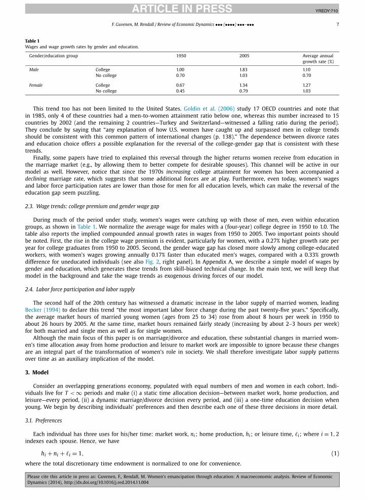
Table 1Wages and wage growth rates by gender and education.
Gender/education group 1950 2005 Average annual growth rate (%)
Male College 1.00 1.83 1.10No college 0.70 1.03 0.70
Female College 0.67 1.34 1.27No college 0.45 0.79 1.03
This trend too has not been limited to the United States. Goldin et al. (2006) study 17 OECD countries and note that in 1985, only 4 of these countries had a men-to-women attainment ratio below one, whereas this number increased to 15 countries by 2002 (and the remaining 2 countries—Turkey and Switzerland—witnessed a falling ratio during the period). They conclude by saying that “any explanation of how U.S. women have caught up and surpassed men in college trends should be consistent with this common pattern of international changes (p. 138).” The dependence between divorce rates and education choice offers a possible explanation for the reversal of the college-gender gap that is consistent with these trends.
Finally, some papers have tried to explained this reversal through the higher returns women receive from education in the marriage market (e.g., by allowing them to better compete for desirable spouses). This channel will be active in our model as well. However, notice that since the 1970s increasing college attainment for women has been accompanied a declining marriage rate, which suggests that some additional forces are at play. Furthermore, even today, women’s wages and labor force participation rates are lower than those for men for all education levels, which can make the reversal of the education gap seem puzzling.
2.3. Wage trends: college premium and gender wage gap
During much of the period under study, women’s wages were catching up with those of men, even within education groups, as shown in Table 1. We normalize the average wage for males with a (four-year) college degree in 1950 to 1.0. The table also reports the implied compounded annual growth rates in wages from 1950 to 2005. Two important points should be noted. First, the rise in the college wage premium is evident, particularly for women, with a 0.27% higher growth rate per year for college graduates from 1950 to 2005. Second, the gender wage gap has closed more slowly among college-educated workers, with women’s wages growing annually 0.17% faster than educated men’s wages, compared with a 0.33% growth difference for uneducated individuals (see also Fig. 2, right panel). In Appendix A, we describe a simple model of wages by gender and education, which generates these trends from skill-biased technical change. In the main text, we will keep that model in the background and take the wage trends as exogenous driving forces of our model.
2.4. Labor force participation and labor supply
The second half of the 20th century has witnessed a dramatic increase in the labor supply of married women, leading Becker (1994) to declare this trend “the most important labor force change during the past twenty-five years.” Specifically, the average market hours of married young women (ages from 25 to 34) rose from about 8 hours per week in 1950 to about 26 hours by 2005. At the same time, market hours remained fairly steady (increasing by about 2–3 hours per week) for both married and single men as well as for single women.
Although the main focus of this paper is on marriage/divorce and education, these substantial changes in married wom-en’s time allocation away from home production and leisure to market work are impossible to ignore because these changes are an integral part of the transformation of women’s role in society. We shall therefore investigate labor supply patterns over time as an auxiliary implication of the model.
3. Model
Consider an overlapping generations economy, populated with equal numbers of men and women in each cohort. Indi-viduals live for T < ∞ periods and make (i) a static time allocation decision—between market work, home production, and leisure—every period, (ii) a dynamic marriage/divorce decision every period, and (iii) a one-time education decision when young. We begin by describing individuals’ preferences and then describe each one of these three decisions in more detail.
3.1. Preferences
Each individual has three uses for his/her time: market work, ni ; home production, hi ; or leisure time, ℓi ; where i = 1, 2indexes each spouse. Hence, we have
hi + ni + ℓi = 1, (1)
where the total discretionary time endowment is normalized to one for convenience.

JID:YREDY AID:710 /FLA [m3G; v1.143-dev; Prn:17/12/2014; 13:01] P.8 (1-26)
8 F. Guvenen, M. Rendall / Review of Economic Dynamics ••• (••••) •••–•••
Spouses derive utility from a composite consumption good, c, which is produced by combining market goods, k, and each spouse’s home production time, hi , according to the following constant elasticity of substitution (CES) technology:
c =(γ kα + (1 − γ )
(A(h1 + h2)
)α) 1α .
Notice that spouses are assumed to be perfectly substitutable in home production, reflecting the view that household chores/tasks can be shared between spouses and performed individually, without requiring much input from the other spouse. This assumption also allows us to generate specialization in market work in a simple fashion: the spouse with a higher wage will work full-time (i.e., h = 0) before the other spouse joins the labor market. With a positive gender wage gap, this mechanism generates a lower labor force participation rate for women than for men, consistent with the data. Although this assumption is not necessary and can be relaxed, it is convenient for generating the significant nonparticipation by married women, especially in the 1950s.
The home production function for singles (including divorced individuals) has the same form but adjusts for the lack of a spouse:
c =(γ kα + (1 − γ )(Ah)α
) 1α .
Individuals are assumed to spend their entire income every period (i.e., no saving technology), so spending on market goods is given by k = (w1n1 + w2n2) for couples and k = wn for singles.13 During marriage, spouses also enjoy the company of each other, which is modeled here as perfect complementarity between spouses’ leisure times: v(ℓ1, ℓ2) = min(ℓ1, ℓ2).14
Although the assumption of perfect complementarity is not necessary—and some substitutability can be allowed for—it simplifies the solution of the model. One empirical motivation for this specification is the well-documented fact that on average, men and women enjoy similar amounts of leisure, which is true not only over time but also across education levels.15
3.1.1. Loves me, loves me notA match-specific, time-varying stochastic term, b, affects the value of the leisure activity: b × min(ℓ1, ℓ2). Its initial
value (when two singles first meet) is drawn from a normal distribution: b0 ∼ N (µb, σ 2b ). During marriage, bt evolves as a
random walk process:
bt+1 = bt + ηt+1, where ηt+1 ∼ N(0,σ 2
η
). (2)
Note that in this formulation, the initial draw b0 has a permanent effect on the value of love during a marriage. Innova-tions during marriage, ηt , have zero mean and variance of σ 2
η . Thus, there is no presumption that bt will always be positive (marital bliss or love)—it can also be negative (marital distress).
To our knowledge, the modeling of love as a term that interacts with a couple’s endogenous decisions is novel to this paper and serves several purposes. First, it captures the adaptable nature of marriage that makes it more resilient to fluctuations in love: couples can mitigate marital distress (bt < 0) by setting ℓ1 = ℓ2 = 0 or further amplify the effects of love through their choices of leisure. With marital distress, spouses get no joy living together but may nevertheless stay married because of the income/home production benefits of marriage.
Second, this specification also implies that how much love matters in marriage depends on the economic environment and alternative uses of time. For example, a couple that struggles financially and therefore has both spouses working long hours would find love to be a luxury that plays a small role in their life. Hence, depending on the choice of parameters, marriages can evolve over time from being mainly productive (i.e., home or market production) to being mainly hedonic (i.e., love and play), as suggested, for example, by Stevenson and Wolfers (2007). We will return to this point in Section 6.4 and measure the extent of this transformation.
3.1.2. Putting the pieces togetherTo summarize, in its most general form, the utility of an individual—whether single, married, or divorced—can be written
as
13 We abstract away from the borrowing-saving decision, for two reasons. The first one is technical: our main focus is on the marriage–divorce decision—which is dynamic—and we chose to enrich that dimension of the model, which is made feasible by limiting other dynamic decisions in the model. Second, while borrowing and saving can serve as an important margin for self insuring against short-term income fluctuations, they are less likely to be effective against large shocks, such as divorce. This is especially true given that the median liquid wealth of US households is less than $5,000, and even smaller at young ages when most of the marriage–divorce decisions take place. Instead, for young households, the substantial portion of lifetime resources is human wealth, which is the main focus of this analysis.14 An alternative interpretation/motivation for this specification is that even if leisure times are not spent jointly, spouses do not enjoy their free time
(guilt?) when their partner has little of it. Or, perhaps, as the old maxim goes: You can never be happier than your spouse—hence the “min” operator.15 For example, Aguiar and Hurst (2007a, Table V) report that, even though men and women have different hours of market work and home production
(which also varies over time and across education levels), when the two components are added, they add up almost to the same figures, leaving both genders to enjoy slightly more than 100 hours of leisure per week.
JID:YREDY AID:710 /FLA [m3G; v1.143-dev; Prn:17/12/2014; 13:01] P.9 (1-26)
F. Guvenen, M. Rendall / Review of Economic Dynamics ••• (••••) •••–••• 9
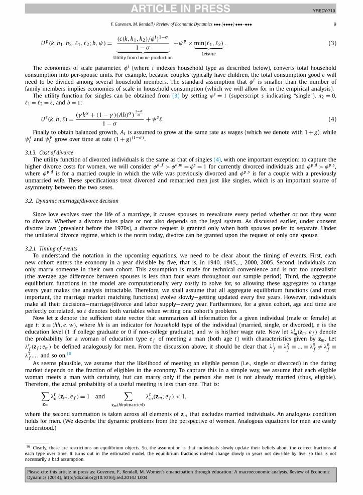
U p(k,h1,h2,ℓ1,ℓ2;b,ψ) = (c(k,h1,h2)/φi)1−σ
1 − σ︸ ︷︷ ︸Utility from home production
+ψ p × min(ℓ1,ℓ2)︸ ︷︷ ︸Leisure
. (3)
The economies of scale parameter, φi (where i indexes household type as described below), converts total household consumption into per-spouse units. For example, because couples typically have children, the total consumption good c will need to be divided among several household members. The standard assumption that φi is smaller than the number of family members implies economies of scale in household consumption (which we will allow for in the empirical analysis).
The utility function for singles can be obtained from (3) by setting φs = 1 (superscript s indicating “single”), n2 = 0, ℓ1 = ℓ2 = ℓ, and b = 1:
U s(k,h,ℓ) = (γ kα + (1 − γ )(Ah)α)1−σα
1 − σ+ ψ sℓ. (4)
Finally to obtain balanced growth, At is assumed to grow at the same rate as wages (which we denote with 1 + g), while ψ s
t and ψ pt grow over time at rate (1 + g)(1−σ ) .
3.1.3. Cost of divorceThe utility function of divorced individuals is the same as that of singles (4), with one important exception: to capture the
higher divorce costs for women, we will consider φd, f > φd,m = φs = 1 for currently divorced individuals and φp,d > φp,s , where φp,d is for a married couple in which the wife was previously divorced and φp,s is for a couple with a previously unmarried wife. These specifications treat divorced and remarried men just like singles, which is an important source of asymmetry between the two sexes.
3.2. Dynamic marriage/divorce decision
Since love evolves over the life of a marriage, it causes spouses to reevaluate every period whether or not they want to divorce. Whether a divorce takes place or not also depends on the legal system. As discussed earlier, under consent divorce laws (prevalent before the 1970s), a divorce request is granted only when both spouses prefer to separate. Under the unilateral divorce regime, which is the norm today, divorce can be granted upon the request of only one spouse.
3.2.1. Timing of eventsTo understand the notation in the upcoming equations, we need to be clear about the timing of events. First, each
new cohort enters the economy in a year divisible by five, that is, in 1940, 1945,..., 2000, 2005. Second, individuals can only marry someone in their own cohort. This assumption is made for technical convenience and is not too unrealistic (the average age difference between spouses is less than four years throughout our sample period). Third, the aggregate equilibrium functions in the model are computationally very costly to solve for, so allowing these aggregates to change every year makes the analysis intractable. Therefore, we shall assume that all aggregate equilibrium functions (and most important, the marriage market matching functions) evolve slowly—getting updated every five years. However, individuals make all their decisions—marriage/divorce and labor supply—every year. Furthermore, for a given cohort, age and time are perfectly correlated, so t denotes both variables when writing one cohort’s problem.
Now let z denote the sufficient state vector that summarizes all information for a given individual (male or female) at age t: z ≡ (hh, e, w), where hh is an indicator for household type of the individual (married, single, or divorced), e is the education level (1 if college graduate or 0 if non-college graduate), and w is his/her wage rate. Now let λt
m(zm; e f ) denote the probability for a woman of education type e f of meeting a man (both age t) with characteristics given by zm . Let λt
f (z f ; em) be defined analogously for men. From the discussion above, it should be clear that λ1f ≡ λ2
f ≡ ... ≡ λ5f = λ6
f ≡λ7
f ... , and so on.16
As seems plausible, we assume that the likelihood of meeting an eligible person (i.e., single or divorced) in the dating market depends on the fraction of eligibles in the economy. To capture this in a simple way, we assume that each eligible woman meets a man with certainty, but can marry only if the person she met is not already married (thus, eligible). Therefore, the actual probability of a useful meeting is less than one. That is:
∑
zm
λtm(zm; e f ) = 1 and
∑
zm(hh=married)
λtm(zm; e f ) < 1,
where the second summation is taken across all elements of zm that excludes married individuals. An analogous condition holds for men. (We describe the dynamic problems from the perspective of women. Analogous equations for men are easily understood.)
16 Clearly, these are restrictions on equilibrium objects. So, the assumption is that individuals slowly update their beliefs about the correct fractions of each type over time. It turns out in the estimated model, the equilibrium fractions indeed change slowly in years not divisible by five, so this is not necessarily a bad assumption.

JID:YREDY AID:710 /FLA [m3G; v1.143-dev; Prn:17/12/2014; 13:01] P.10 (1-26)
10 F. Guvenen, M. Rendall / Review of Economic Dynamics ••• (••••) •••–•••
3.2.2. Assortative meetingWe allow the meeting rates of individuals by education level to differ from what would be implied by purely random
meetings across all individuals. Specifically, let θeme fm > 0 be a scaling factor that drives a wedge between the population
fraction of males with education em and the probability that a woman with education e f meets such males. Similarly, let θ
e f em
f be the analogous scaling factor for men. The probability of a woman with education e f meeting a man with education em is
λtm(zm; e f ) = θ
eme fm × P t
m(zm),
where P tm(zm) denotes the population fraction of men with characteristics zm at age t . Assortative meeting means θ11
m > 1. We also assume that the probabilities for the same type of women meeting uneducated men are scaled down appropriately, so that the probabilities add up to one. That is,
θ01m ≡
1 − ∑zm,em=1[θ11
m × P tm(zm)]
∑zm,em=0[P t
m(zm)] .
Finally, the population fractions of each group in equilibrium also impose the following restriction: θeme fm ×
max(P tm, P t
f ) ≤ 1.17
3.2.3. Value functions and decision thresholdsFirst, substituting the static optimal choices (for leisure as well as home and market hours) into the period utility func-
tions (3) or (4) yields indirect utility functions, which we denote with V s(w f ), V d(w f ; φd, f ) for single and divorced women, respectively, and V p(b, zm; z f , φp) for married couples. Notice that a married couple’s (static) indirect utility depends on the relevant economies of scale, which itself depends on each spouse’s marital history.
Now, let J f (b, zm; z f , λtm) denote the value function of a woman with characteristics z f married to a man with charac-
teristics zm when the love level is b. Further, let S f (z f , λtm) denote the value function of the same individual when single
and D f (z f , λtm) when divorced.18 (It is understood that the component of z denoting partnership status matches up with
the value function type in each case.)Now let b f (zm; z f ) denote the threshold level of love, above which a woman with characteristics z f prefers to marry a
man of type zm over staying single. Formally:
b f (zm; z f ) = min b s.t. J f (b, zm; z f ,λtm)≥ S f (z f ,λ
tm).
Let bm(z f ; zm) denote the analogous threshold for the man who meets the very same (type of) woman. Clearly, the two thresholds can differ. We assume that a meeting turns into a marriage if both potential spouses prefer marriage over being single. So, let B p(z f , zm) ≡ max(bm, b f ) be the threshold that determines the marriage between these two individuals. Similarly, we can define thresholds for married individuals contemplating divorce. Specifically, for the wife:
bd, f (zm; z f ) = min b s.t. J f (b, zm; z f ,λtm)≥ D f (z f ,λ
tm);
and bd,m(z f ; zm) is analogously defined for her husband.
3.2.4. When does divorce take place?Unlike marriage, divorce does not always require both spouses’ agreement. In the consent regime, both spouses must
jointly want to divorce, so the divorce threshold is determined by the spouse that is more willing to remain married:
Bcd(z f , zm) = min(bd,m,bd, f ),
where the superscript “cd” stands for “consent divorce.” In the unilateral regime, the divorce threshold for love has the same form as the marriage threshold, but with different arguments:
Bud(z f , zm) ≡ max(bd,m,bd, f ),
where the superscript “ud” stands for “unilateral divorce.”19 Therefore, as soon as marital bliss falls below this threshold, the spouse with the higher love threshold would file for, and be granted, a divorce. Other variables are defined analogously.
17 To see why this condition is needed, suppose, for example, that there are 100 males and 100 females, with 20 educated males and 30 educated females. Assuming that each educated female meets an educated male with a probability higher than 66.6% is not meaningful. To be consistent with this assumption, there would need to be more than 20 educated males or more than one meeting per period, neither of which we allow. An analogous condition from the men’s perspective must also be satisfied. Both of these sets of conditions are satisfied when the condition given in the text holds.18 Notice that the two value functions will not be identical, i.e., S f ≡ D f , even when φd = φ , because a divorced individual has to wait before he/she can
reenter the marriage market.19 Notice again that even when φd, f = φs = 1, we would not have Bud = B p for the same reason explained in footnote 18.
JID:YREDY AID:710 /FLA [m3G; v1.143-dev; Prn:17/12/2014; 13:01] P.11 (1-26)
F. Guvenen, M. Rendall / Review of Economic Dynamics ••• (••••) •••–••• 11
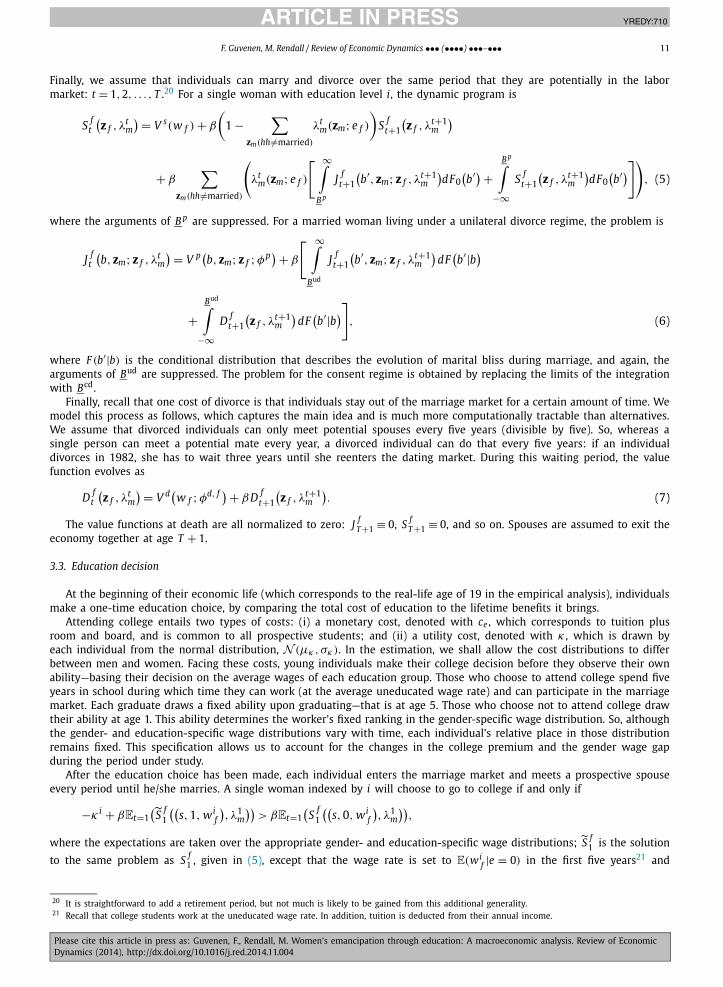
Finally, we assume that individuals can marry and divorce over the same period that they are potentially in the labor market: t = 1, 2, . . . , T .20 For a single woman with education level i, the dynamic program is
S ft(z f ,λ
tm)= V s(w f ) + β
(1 −
∑
zm(hh=married)
λtm(zm; e f )
)S f
t+1
(z f ,λ
t+1m
)
+ β∑
zm(hh=married)
(
λtm(zm; e f )
[ ∞∫
B p
J ft+1
(b′, zm; z f ,λ
t+1m
)dF0
(b′) +
B p∫
−∞S f
t+1
(z f ,λ
t+1m
)dF0
(b′)
])
, (5)
where the arguments of B p are suppressed. For a married woman living under a unilateral divorce regime, the problem is
J ft(b, zm; z f ,λ
tm)= V p(
b, zm; z f ;φp)+ β
[ ∞∫
Bud
J ft+1
(b′, zm; z f ,λ
t+1m
)dF
(b′|b
)
+Bud∫
−∞D f
t+1
(z f ,λ
t+1m
)dF
(b′|b
)]
, (6)
where F (b′|b) is the conditional distribution that describes the evolution of marital bliss during marriage, and again, the arguments of Bud are suppressed. The problem for the consent regime is obtained by replacing the limits of the integration with Bcd.
Finally, recall that one cost of divorce is that individuals stay out of the marriage market for a certain amount of time. We model this process as follows, which captures the main idea and is much more computationally tractable than alternatives. We assume that divorced individuals can only meet potential spouses every five years (divisible by five). So, whereas a single person can meet a potential mate every year, a divorced individual can do that every five years: if an individual divorces in 1982, she has to wait three years until she reenters the dating market. During this waiting period, the value function evolves as
D ft(z f ,λ
tm)= V d(w f ;φd, f ) + βD f
t+1
(z f ,λ
t+1m
). (7)
The value functions at death are all normalized to zero: J fT +1 ≡ 0, S f
T +1 ≡ 0, and so on. Spouses are assumed to exit the economy together at age T + 1.
3.3. Education decision
At the beginning of their economic life (which corresponds to the real-life age of 19 in the empirical analysis), individuals make a one-time education choice, by comparing the total cost of education to the lifetime benefits it brings.
Attending college entails two types of costs: (i) a monetary cost, denoted with ce , which corresponds to tuition plus room and board, and is common to all prospective students; and (ii) a utility cost, denoted with κ , which is drawn by each individual from the normal distribution, N (µκ , σκ ). In the estimation, we shall allow the cost distributions to differ between men and women. Facing these costs, young individuals make their college decision before they observe their own ability—basing their decision on the average wages of each education group. Those who choose to attend college spend five years in school during which time they can work (at the average uneducated wage rate) and can participate in the marriage market. Each graduate draws a fixed ability upon graduating—that is at age 5. Those who choose not to attend college draw their ability at age 1. This ability determines the worker’s fixed ranking in the gender-specific wage distribution. So, although the gender- and education-specific wage distributions vary with time, each individual’s relative place in those distribution remains fixed. This specification allows us to account for the changes in the college premium and the gender wage gap during the period under study.
After the education choice has been made, each individual enters the marriage market and meets a prospective spouse every period until he/she marries. A single woman indexed by i will choose to go to college if and only if
−κ i + βEt=1(
S f1
((s,1, wi
f
),λ1
m))
> βEt=1(
S f1
((s,0, wi
f
),λ1
m))
,
where the expectations are taken over the appropriate gender- and education-specific wage distributions; S f1 is the solution
to the same problem as S f1 , given in (5), except that the wage rate is set to E(wi
f |e = 0) in the first five years21 and
20 It is straightforward to add a retirement period, but not much is likely to be gained from this additional generality.21 Recall that college students work at the uneducated wage rate. In addition, tuition is deducted from their annual income.

JID:YREDY AID:710 /FLA [m3G; v1.143-dev; Prn:17/12/2014; 13:01] P.12 (1-26)
12 F. Guvenen, M. Rendall / Review of Economic Dynamics ••• (••••) •••–•••
Fig. 3. Timing of events.
then switches to the stochastic draw, wif , from the wage distribution of educated workers. The terms on the left-hand
side represent the lifetime utility if a young woman gets a college degree, and the right-hand side represents the same if she does not. It is clear that the future benefit of education depends on both (i) the average wages of college graduates versus high school graduates, and (ii) the marriage market prospects of both education groups, which can be seen by the dependence of the value function on λ1
m . Finally, to be consistent with balanced growth, the utility cost κ is assumed to grow at the annual rate of (1 + g)(1−σ ) .
Note that if n2 > 0, the prospective secondary worker’s wage matters to the primary earner, since it does contribute to family resources. In this case, if women have lower wages, education not only benefits women when they are single but also makes them more desirable spouses. Thus, educated women will have a higher divorce threshold, since their outside option (determined both by their wage as single women and by their subsequent marriage prospects) looks better. We will return to this mechanism in Section 6.4. Therefore, as education rises, the same variance of so-called love shocks may lead to more divorces. A rise in returns to human capital should then increase female education demand more so than male education even in the face of lower returns to education. The divorce rate and female labor force participation should also rise.
Fig. 3 summarizes the timing of events over the life cycle.
3.4. Equilibrium in the marriage market
This basic framework generates several interesting feedbacks between the education choice and marriage/divorce deci-sions. One mechanism that we are particularly interested in is the following. Suppose that in the 1950s, women come to expect that the divorce law will change in the future.
First, it is instructive to examine what happens mechanically with an exogenous change from consent to unilateral divorce law in this model. Consent divorce law requires b < min(bd,m, bd, f ), whereas unilateral divorce requires only b <max(bd,m, bd, f ), which implies that the divorce rate will rise quickly after the change in the law (from consent to unilateral), consistent with what has been observed in the US data during the 1970s. However, because the new marriages formed under the unilateral law will involve better selection, the rise in the divorce rate is followed with a subsequent but smaller decline.
Second, since education provides insurance against divorce (in the form of higher income), the expectation of changing divorce risk will increase the demand for education for young women in the 1950s. (Although these effects are similar for men, they are not symmetric—both because of the different costs of divorce by gender and because of the gender wage gap.) But higher income in turn reduces an important benefit of marriage for women, by closing the income gap between the spouses, which then—now endogenously—raises the divorce rate. This happens because women search longer for a suitable match and married women who previously did not agree to divorce (despite a low value of b) are now willing to divorce and stay single since, they are able to support themselves with their higher income. The amplification mechanism means that an exogenous rise in divorce risk (change in divorce regime) can result in a larger rise in actual divorce rates as well as in women’s educational attainment in equilibrium. However, in equilibrium this does not imply that educated marriages are more unstable. The contrary is true, as educated marriages benefit from better initial selection.
Finally, the interaction of education and the marriage market also creates an externality effect: when there are more educated men than women, some educated men are likely to marry uneducated women (rather than remain single), which

JID:YREDY AID:710 /FLA [m3G; v1.143-dev; Prn:17/12/2014; 13:01] P.13 (1-26)
F. Guvenen, M. Rendall / Review of Economic Dynamics ••• (••••) •••–••• 13
Table 2Economies of scale by household type.
Single 1st marriage Divorced 2nd + marriage
Woman 1.0 2.36 1.64 2.71Man 1.0 2.36 1.0 2.36 (w/single)
2.71 (w/divorced)
Note: The computation from the SIPP yields values for φ of 1.08 for divorced man, 1.18 for single woman, and 1.07 for single man. We round these figures down to 1.0 to keep track of fewer numbers.
lowers the returns on education for women. However, as more women get educated, attracting an educated man becomes more difficult for an uneducated woman, which increases the education demand of all women. Thus, the returns to educa-tion can easily be increasing in the supply of educated women, which fuels demand for education. Therefore, a change in quality of the marriage market toward high education can lead to an increase in women’s educational attainment.22
4. Econometric analysis
We conduct the empirical analysis in two stages. In the first step, we fix some parameters based on external estimates. Then in the second step, we estimate the remaining parameters by matching a variety of data moments using method of simulated moments (MSM).
4.1. First stage
A model period corresponds to one year of calendar time. As noted earlier, individuals are economically active between ages 20 and 64 (i.e., for 45 model periods). We set β = 0.98, α = 0.45 (Aguiar and Hurst, 2007a), and ce = 0.105. The tuition cost is equal to one-third of average educated wage earnings, taking into account average hours worked.23
The empirical wage distributions that are fed into the structural model are obtained by fitting lognormal distributions to each year of the CPS data, separately for each education and gender group and then computing five-year moving averages. As for the growth rate of wages, g , the US data show a clear trend break around 1975, so a constant growth rate seems grossly counterfactual. Therefore, we set g = 1.87% (computed from 1950 to 1974) per year before that date and g = 0%(1985–2005 average) after that date (including into the future after 2005). Furthermore, the gender- and education-specific wages are assumed to grow at the 1980–2005 average rate into the future.24
4.1.1. Economies of scaleAn important set of parameters in the model measures the economies of scale for different household types. Following
much of the literature, we measure economies of scale using the number of adults and children in a household. In particular, we take the view that the cost of divorce is heavily influenced by the presence of children, who have to be cared for when spouses are divorced, as well as cared for in newly formed households by the biological parents and stepparents in the case of remarriage. To this end, we use the Survey of Income and Program Participation (SIPP) to compute the number of children living in a household for previously divorced versus never-divorced couples (of women ages 20–34). Moreover, the data also allow us to distinguish between biological and stepchildren. The economies of scales computed from the SIPP are detailed in Appendix C. The resulting economies of scale parameters are φp,s = 2.36 for married households in which the wife was previously never married (regardless of the husband’s history), φp,d = 2.71 for married households with a previously divorced woman, and φd, f = 1.64 for currently divorced women.25 As discussed in Appendix C.2, since remarriage is non-random with respect to the number of children, divorced women who end up remarrying have fewer children, the 2.71 figure for φp,d is based on the number of children who live in a household in which the mother was a previously divorced woman. Table 2 summarizes the relevant values for the benchmark model.
Finally, notice that the choice for φp,d implies that divorce has a permanent cost that extends into subsequent marriages. This assumption reflects the view once succinctly summarized by novelist Nora Ephron, who famously said that “marriages come and go, but divorce is forever.” For comparison, we also explore the view that the suffering from divorce ends once somebody remarries: e.g., φp,d = φp,s = 2.36. We shall refer to this version as the temporary divorce cost model (hereafter, the TDC model).
22 As can be anticipated from this discussion, this framework is open to the possibility of multiple equilibria, although this is nothing new in search models of the marriage market. We have not detected any signs that this posed a problem in the neighborhood of the parameter space around the estimated parameter vector (despite careful investigation), this issue still requires care.23 This number is in line with Gallipoli et al. (2010), who report a figure of 30% of median labor earnings.24 Because there is no capital accumulation, and in fact the only dynamic decisions are marriage/divorce and education, the change in the balanced growth
path does not present any technical challenges.25 Since in the US data most children live with their mother, economies of scale for divorced men are close to one. For simplicity we therefore set the
economies of divorced men equal to those for single, never married men and women, φ = 1, and the economies of scale for remarried divorced men equal to those for married couples who have never been divorced.

JID:YREDY AID:710 /FLA [m3G; v1.143-dev; Prn:17/12/2014; 13:01] P.14 (1-26)
14 F. Guvenen, M. Rendall / Review of Economic Dynamics ••• (••••) •••–•••
Table 3Estimated structural parameters.
Parameters Benchmark MFD TDC(1) (2) (3)
σ (Curvature on cons. composite) 1.29 1.02 1.34(0.005) (0.042) (0.011)
γ (Weight on market consumption) 0.58 0.60 0.59(0.002) (0.003) (0.001)
ψ s (Leisure weight for singles) 2.15 2.24 2.65(0.016) (0.199) (0.059)
θ11m (Degree of assortative matching) 2.96 2.59 2.48
(0.004) (0.102) (0.059)
µb (Mean of initial love draw) 1.36 −1.70 1.26(0.022) (0.261) (0.179)
σb (Std. dev. of initial love draw) 0.69 3.06 4.26(0.010) (0.158) (0.144)
ση (Std. dev. of love innovation) 1.33 1.78 3.03(0.011) (0.156) (0.082)
µmκ (Men’s mean psychic cost of educ.) 15.70 12.01 19.18
(0.207) (1.226) (0.647)
µ fκ (Women’s mean psychic cost of educ.) 17.75 12.40 16.41
(0.175) (0.758) (0.533)
σκ (Std. dev. of psychic cost) 10.85 7.25 9.54(0.17) (0.443) (0.370)
Objective value 10.55 20.49 36.59
Notes: Standard errors are in parentheses. See Section 7.4 for descriptions of the MFD and TDC models.
Before closing this discussion a remark is in order. So far, we have interpreted differences in φ as reflecting differences in childrearing costs. This brings up the question: If divorced individuals suffer because raising children is more costly, then why do individuals not respond to higher divorce risk by having fewer children? This could provide another margin for insuring against divorce. While it is certainly feasible, it is not clear that going from three children down to two reduces childrearing costs substantially, and going down all the way to no children could entail much larger (utility) losses for many couples than simply obtaining education. Thus, in this paper, we shall view fertility as a margin that is sufficiently costly to adjust that it is not being used as a source of insurance.26
4.1.2. Cohort size variationCohort sizes vary over time to capture the baby boom and other variations observed in the US data. This variation could
be important because the propensity to marry and divorce clearly varies over the life cycle and, as the age composition of the population changes over time, this could create changes in marriage and divorce patterns, which we wish to account for. Furthermore, in our analysis below, we focus on individuals ages 20–34 so as to further mitigate changing age structure on observed statistics. Notice that because marriage is only allowed within cohorts, there is no explicit dependence (i.e., general equilibrium feedbacks) across cohorts.
4.1.3. Divorce laws and expectationsIndividuals live under a consent law regime until 1975 and then switch to an unilateral regime. Before 1950, the economy
grows along a balanced growth path where individuals expect to remain in a consent regime in the future. Expectations change after 1950, and individuals become aware of the future reform as well as the future path of wages. We also examine the results under myopic expectations regarding both wages and divorce reform. The non-stationary changes in the economy (including those in wages) last from 1950 to 2005, after which time wages revert to growing at a constant rate, leading to a new balanced growth path equilibrium once the cohorts that entered the economy in 2005 exit (in 2050).
4.2. Second stage: MSM estimation
The remaining parameters (see Table 3 for a detailed description) are estimated by matching a number of important moments of the US data. Specifically, the structural parameters to be estimated are stacked in a q × 1 vector:
θ ≡[σ ,γ ,ψ s, θee,µb,σb,σζ ,µm
κ ,µ fκ ,σκ
]′.
Let m(X) be an R × 1 vector of data moments (with R > q) and let f(Xsim(θ)) be the same moments obtained from the simulated data of the economic model where the structural parameter vector is given by θ . More specifically, we have
26 Furthermore, a higher φ for divorced individuals also captures other costs of divorce, such as stigma in the marriage market, psychological costs associated with divorce, and so on. Although it would be interesting to analyze how variation in such costs over time effects our results, such costs are difficult to measure directly, and we leave that for future work.
JID:YREDY AID:710 /FLA [m3G; v1.143-dev; Prn:17/12/2014; 13:01] P.15 (1-26)
F. Guvenen, M. Rendall / Review of Economic Dynamics ••• (••••) •••–••• 15
m =
⎡
⎢⎢⎢⎣
m1(X)
m2(X)
...
mR(X)
⎤
⎥⎥⎥⎦f(θ) =
⎡
⎢⎢⎢⎣
f1(Xsim(θ))
f2(Xsim(θ))
...
f R(Xsim(θ))
⎤
⎥⎥⎥⎦.
Under the null hypothesis that the structural model is correctly specified, we have R moment conditions: E(m −f(Xsim(θ0))) = 0. The MSM estimator is
θ = arg max[m − f
(Xsim(θ)
)]′W[m − f
(Xsim(θ)
)].
We choose the weighting matrix, W, such that the objective function is the squared sum of percentage deviations be-tween the model and the data moments.27 The 10-element vector of structural parameters is estimated by matching 12 empirical moments of the US data. Ten of these moments pertain to 2005 and two of them pertain to 1950. All moments are computed for young individuals. For most of the moments studied in this paper, we take these to be individuals ages 20 to 34. The only exception is the labor supply of young workers, which we compute for 25- to 34-year-old individuals (because many of those younger than 25 are still in school). The moment conditions in m are as follows:
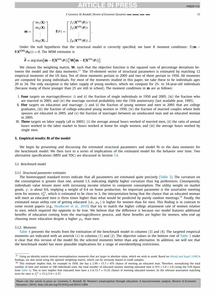
I. Four targets on marriage/divorce: (i and ii) the fraction of single individuals in 1950 and 2005, (iii) the fraction who are married in 2005, and (iv) the marriage survival probability into the 15th anniversary (last available year, 1995).
II. Five targets on education and marriage: (i and ii) the fraction of young women and men in 2005 that are college graduates, (iii) the fraction of college-educated young women in 1950, (iv) the fraction of married couples where both spouses are educated in 2005, and (v) the fraction of marriages between an uneducated man and an educated woman in 2005.
III. Three targets on labor supply (all in 2005): (i) the average annual hours worked of married men, (ii) the ratio of annual hours worked in the labor market to hours worked at home for single women, and (iii) the average hours worked by single men.
5. Empirical results: fit of the model
We begin by presenting and discussing the estimated structural parameters and model fit to the data moments for the benchmark model. We then turn to a series of implications of the estimated model for the behavior over time. Two alternative specifications (MFD and TDC) are discussed in Section 7.4.
5.1. Benchmark model
5.1.1. Structural parameter estimatesThe bootstrapped standard errors indicate that all parameters are estimated quite precisely (Table 3). The curvature on
the consumption is greater than one, around 1.3, indicating slightly higher curvature than log preferences. Consequently, individuals value leisure more with increasing income relative to composite consumption. The utility weight on market goods, γ , is about 0.6, implying a weight of 0.4 on home production. An important parameter is the assortative meeting term for women, θ11
m , which is estimated to be close to 3, the interpretation being that the chance that an educated woman will meet an educated men is three times higher than what would be predicted by purely random meetings.28 Finally, the estimated mean utility cost of getting educated (i.e., µκ ) is higher for women than for men. This finding is in contrast to some recent papers (e.g., Heathcote et al., 2010) that try to match the higher college attainment rate of women relative to men, which required the opposite to be true. We believe that the difference is because our model features additional benefits of education coming from the marriage/divorce process, and these benefits are higher for women, who end up choosing more education despite a higher µκ than men.
5.1.2. MomentsTable 4 presents the results from the estimation of the benchmark model in columns (3) and (4). The targeted empirical
moments are indicated with an asterisk (∗) in columns (1) and (2). The objective values in the bottom row of Table 3 make it clear that this version of the model fits the selected moments better than any alternative. In addition, we will see that the benchmark model has more plausible implications for a range of overidentifying restrictions.
27 Using an identity matrix instead overemphasizes moments that are larger in absolute value, which we wish to avoid. Based on Altonji and Segal (1996)’s findings, we also avoid using the optimal weighting matrix, which can be seriously biased in small samples.28 This estimate implies that, for example in 1950, she has a 2.99 × 15.7 = 47% chance of meeting an educated man. Therefore, normalizing the total
number of men and women to 100 individuals each, the total number of educated women meeting educated men is 47% × 5.9 = 2.8 (using the 5.9% figure from Table 4). This in turn implies that educated men have a 2.4/15.7 = 15.2% chance of meeting educated women. So the relevant assortative matching term for men is θ11
f = 15.2/5.9 ≈ 2.57.

JID:YREDY AID:710 /FLA [m3G; v1.143-dev; Prn:17/12/2014; 13:01] P.16 (1-26)
16 F. Guvenen, M. Rendall / Review of Economic Dynamics ••• (••••) •••–•••
Table 4Key moments: US data vs. estimated structural model.
US data Benchmark Counterfactual: no divorce reform
1950 2005 1950 2005 2005(1) (2) (3) (4) (5)
Fraction single 20.6* 47.8* 23.1 46.3 25.2Fraction divorced 3.0a 7.5* 0.0 8.7 0.0Fraction ever divorced (30–34) 17.4 0.0 19.7 0.0Divorce rate 2.4b 3.4b 0.0 3.8 0.0Survival to 15th anniversary 86.7 63.7* 99.9 57.0 99.9Fraction married 75.1 44.8 76.9 44.9 74.7Marriage rate 24.0b 9.5b 20.9 9.0 19.7
Young educ. women 5.9* 33.0* 6.0 33.4 19.2Young educ. men 9.6 28.7* 16.1 29.1 33.2
Couples ed./ed. 3.1 21.5* 2.7 24.3 16.0Couples ed./uned. 6.8 8.4 15.4 6.3 17.9Couples uned./ed. 1.7 10.5* 3.4 11.4 1.5Couples uned./uned. 88.5 59.7 78.4 58.1 64.6
Married male hours 42.3 42.0* 64.3 39.2 57.3Single male hours 34.5 36.1* 36.9 38.2 37.3Married female hours 8.1 26.2 6.7 23.4 14.3Single female hours 29.2 32.2 34.2 36.8 35.3Single female market/home hours 1.20* 0.94 1.04 1.02
Notes: All cells in the top two panels report results in percentage terms. The bottom panel reports results in hours per week. The last line is a ratio.* Moments targeted in the MSM estimation.a The fraction divorced for young in 1940 is 1.7% and in 1960 it is 4.4%. The cell reports the average of these two figures.b Moments computed for 1968 (instead of 1950) and 1995 (instead of 2005) due to data availability.
We begin with the moments related to marriage and divorce. The fraction of young individuals that are single is 47.8% in the US data in 2005, which the model matches well (46.3%). Similarly, singles make up 20.6% of the population in the data in 1950 and this figure is matched fairly well (23.1%) by the model.
Turning to divorces, we see that the fraction who are divorced is 7.5% in the data compared to 8.7% in the model. The model also does a reasonable job of matching related statistics on divorce rates—the fraction of 30- to 34-year-olds who were ever divorced (17.4% vs. 19.7%) and the divorce rate in 2005 (3.4% vs. 3.8%). But it understates the divorce rate in 1950, which we discuss further below. Third, and finally, an important moment that helps us pin down the dynamics of marriage and divorce is the fraction of marriages that survive into the 15th anniversary. This figure is 63.7% in the data vs. 57.0% in the model.
The second important dimension of the data concerns educational attainment. The model matches all three educational attainment targets—the fractions of young educated females in 2005 and 1950 and the fraction of young educated males in 2005. This good fit was facilitated by the fact that the model has three parameters that are directly linked to the cost of education (µm
κ , µ fκ , σκ ) and have little other impact on any other dimension of the model. Turning to the interaction of
education and marriage, we see that the calibration targeted two types of couples by education level: first, the fraction of couples in which both spouses are educated and, second, the fraction of couples with an uneducated male and educated female. Both targets are matched well: the former fraction is 21.5% in the data and 24.3% in the model, and the latter is 10.5% in the data and 11.4% in the model.
Third, we turn to labor supply. For both married and single males, the model broadly matches the empirical targets, whereas for single females the model slightly underpredicts the ratio of market to home production hours: the ratio is 1.20 in the data versus 1.04 in the model. Among the non-targeted moments, the married female hours is a bit understated (26.2 vs. 23.4 hours per week), whereas the single female hours is overstated (32.2 vs. 36.8).
6. Trends over time
After having verified that the model does a fairly good job of matching the data targets in 2005, we now turn to the main question of interest: How well does the model perform in explaining key empirical trends over time? Two of these trends will be fit by design—e.g., choice of moments in the estimation. The rest will serve as overidentifying restrictions of the model.
6.1. Marriage and divorce
The model generates patterns that are qualitatively consistent with the trends in the data: a rise in the fractions of singles and divorced individuals, and a fall in the fraction of married individuals and in the survival probability of marriages to the 15th anniversary. Before delving into the details, we note that (perhaps contrary to what it might seem) the rising
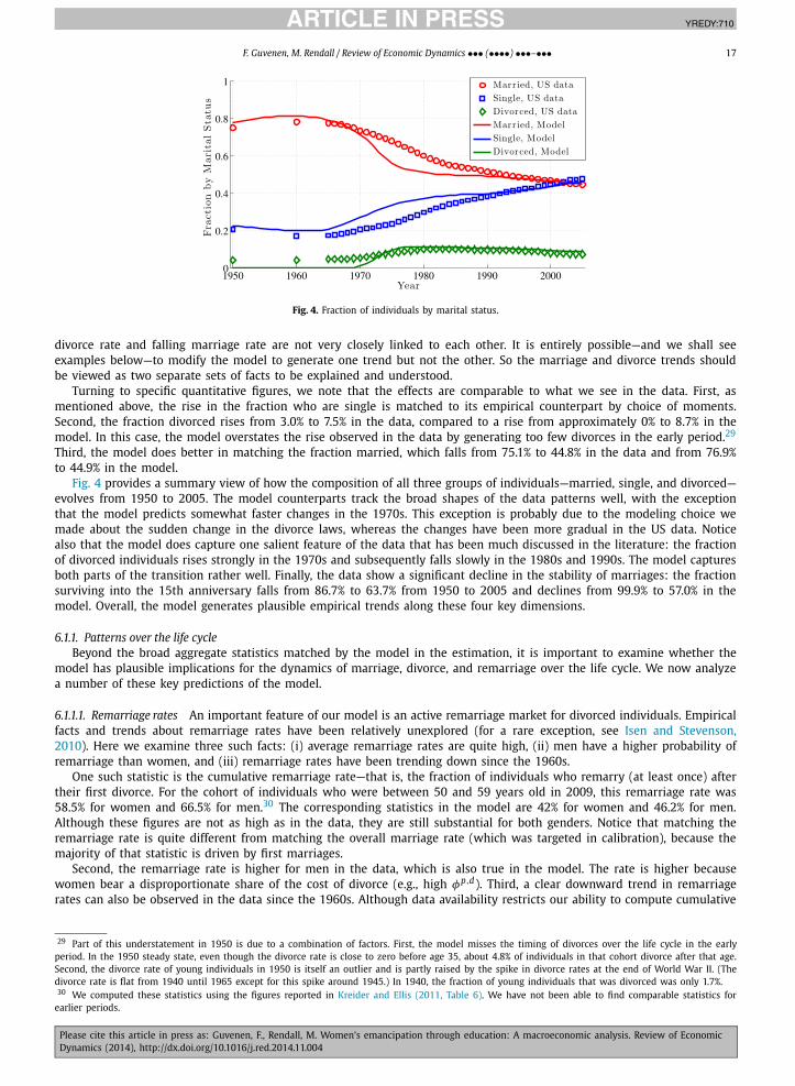
JID:YREDY AID:710 /FLA [m3G; v1.143-dev; Prn:17/12/2014; 13:01] P.17 (1-26)
F. Guvenen, M. Rendall / Review of Economic Dynamics ••• (••••) •••–••• 17
Fig. 4. Fraction of individuals by marital status.
divorce rate and falling marriage rate are not very closely linked to each other. It is entirely possible—and we shall see examples below—to modify the model to generate one trend but not the other. So the marriage and divorce trends should be viewed as two separate sets of facts to be explained and understood.
Turning to specific quantitative figures, we note that the effects are comparable to what we see in the data. First, as mentioned above, the rise in the fraction who are single is matched to its empirical counterpart by choice of moments. Second, the fraction divorced rises from 3.0% to 7.5% in the data, compared to a rise from approximately 0% to 8.7% in the model. In this case, the model overstates the rise observed in the data by generating too few divorces in the early period.29
Third, the model does better in matching the fraction married, which falls from 75.1% to 44.8% in the data and from 76.9% to 44.9% in the model.
Fig. 4 provides a summary view of how the composition of all three groups of individuals—married, single, and divorced—evolves from 1950 to 2005. The model counterparts track the broad shapes of the data patterns well, with the exception that the model predicts somewhat faster changes in the 1970s. This exception is probably due to the modeling choice we made about the sudden change in the divorce laws, whereas the changes have been more gradual in the US data. Notice also that the model does capture one salient feature of the data that has been much discussed in the literature: the fraction of divorced individuals rises strongly in the 1970s and subsequently falls slowly in the 1980s and 1990s. The model captures both parts of the transition rather well. Finally, the data show a significant decline in the stability of marriages: the fraction surviving into the 15th anniversary falls from 86.7% to 63.7% from 1950 to 2005 and declines from 99.9% to 57.0% in the model. Overall, the model generates plausible empirical trends along these four key dimensions.
6.1.1. Patterns over the life cycleBeyond the broad aggregate statistics matched by the model in the estimation, it is important to examine whether the
model has plausible implications for the dynamics of marriage, divorce, and remarriage over the life cycle. We now analyze a number of these key predictions of the model.
6.1.1.1. Remarriage rates An important feature of our model is an active remarriage market for divorced individuals. Empirical facts and trends about remarriage rates have been relatively unexplored (for a rare exception, see Isen and Stevenson, 2010). Here we examine three such facts: (i) average remarriage rates are quite high, (ii) men have a higher probability of remarriage than women, and (iii) remarriage rates have been trending down since the 1960s.
One such statistic is the cumulative remarriage rate—that is, the fraction of individuals who remarry (at least once) after their first divorce. For the cohort of individuals who were between 50 and 59 years old in 2009, this remarriage rate was 58.5% for women and 66.5% for men.30 The corresponding statistics in the model are 42% for women and 46.2% for men. Although these figures are not as high as in the data, they are still substantial for both genders. Notice that matching the remarriage rate is quite different from matching the overall marriage rate (which was targeted in calibration), because the majority of that statistic is driven by first marriages.
Second, the remarriage rate is higher for men in the data, which is also true in the model. The rate is higher because women bear a disproportionate share of the cost of divorce (e.g., high φp,d). Third, a clear downward trend in remarriage rates can also be observed in the data since the 1960s. Although data availability restricts our ability to compute cumulative
29 Part of this understatement in 1950 is due to a combination of factors. First, the model misses the timing of divorces over the life cycle in the early period. In the 1950 steady state, even though the divorce rate is close to zero before age 35, about 4.8% of individuals in that cohort divorce after that age. Second, the divorce rate of young individuals in 1950 is itself an outlier and is partly raised by the spike in divorce rates at the end of World War II. (The divorce rate is flat from 1940 until 1965 except for this spike around 1945.) In 1940, the fraction of young individuals that was divorced was only 1.7%.30 We computed these statistics using the figures reported in Kreider and Ellis (2011, Table 6). We have not been able to find comparable statistics for
earlier periods.

JID:YREDY AID:710 /FLA [m3G; v1.143-dev; Prn:17/12/2014; 13:01] P.18 (1-26)
18 F. Guvenen, M. Rendall / Review of Economic Dynamics ••• (••••) •••–•••
Table 5Annual remarriage rates by gender, 1975–2005.
Year Female Male
Data Model Data Model
1975 188 118 266 1311985 163 107 177 1141995 106 96 107 1012005 92 91 98 96
Table 6Life cycle patterns in marriage and divorce.
Median statistics US data Model
Age at first marriage (1960/2010)Men 24/28.5 23/28Women 21/27 23/27
Duration of first marriage for those who divorced 8 8Duration between first divorce and remarriage or those who divorced/remarried 3.8 10Fraction never-married women by age 59 (1986/2004) 4.2/9.5 4.9/8.6Fraction ever-divorced women of those ever-married (2004) 44.1 55.9
Note: US data statistics are from the Census Bureau.
remarriage rates in earlier periods, we can compute annual remarriage rates going back to the 1970s using SIPP Wave 2 modules. Table 5 reports the figures from US data and from the model per 1000 divorced women. The features emphasized above can also be seen here for the annual rates—the downward trend in remarriage rates and the fact that men have higher remarriage rates than women.31
6.1.1.2. Age patterns in marriage and divorce A well-documented trend has been the gradual rise in the median age of first marriage since the middle of the 20th century.32 For men, the median age rose almost monotonically from 24 years in 1960 to 28.5 years in 2010 (Table 6). For women, the median age rose from 21 years to 27 years. Similarly, in the model, the median age climbs from 23 years for both genders in 1960 to 28 years in 2005 for men and 27 years for women.
6.1.1.3. Duration of marital states Next, we turn to the durations of various marital states that individuals go through. The Census Bureau reports that in 2009, the “median duration of first marriage for those whose first marriage ended in divorce” was 8.0 years for both men and women. The corresponding number is precisely 8 years in our model. Another relevant statistic concerns the time it takes individuals to remarry. Again, the Census Bureau reports that the “median duration between first divorce and remarriage for those whose first marriages ended in divorce and who had remarried” was 3.8 years for both men and women in the US data. The corresponding figure is quite a bit longer—10 years—in our baseline model. This is largely because we assume divorced individuals participate in the marriage market every 5 years, which extends the duration they remain divorced.33
Finally, another statistic of interest is the fraction of individuals who never marry (which we take to mean up to age 59). This figure has increased from 4.2% in 1960 to 9.5% in 2010 for women (Kreider and Ellis, 2011, Table 2). The model counterpart is similar: it rises from 4.9% to 8.6% during the same period. A different statistic of this sort is the fraction of ever-married women that divorce at least once. The fraction is reported in the same source to be 44.1% for women 45 to 55 years of age in the year 2004. The same statistic in 2005 is 55.9% in our model. Although the match is clearly not perfect, the model is consistent with the rough magnitudes in the data.
Collectively, these results show that the estimated structural model makes plausible predictions for important aspects of the marriage/divorce/remarriage process that are not directly targeted in the estimation, as well as for how these behaviors changed over time.
6.2. Education trends
6.2.1. Reversal of the college-gender gapWe now turn to the reversal of the college-gender gap, which happened during the 1990s. Recall that the estimation
targeted educational attainment rates for men and women in 2005 and for women in 1950 (see Table 4). Thus, the model matches—by construction—the fact that women have a higher college attainment rate than men in 2005. The question then is: Do we see the opposite pattern in 1950? The answer is “yes.”
31 These findings are consistent with the five-year remarriage rates reported in Kreider (2006).32 Source: Elliott et al. (2012). The available decennial census data goes back to 1890 and show a slight decline in the median age until 1950.33 Shortening this duration to reentry is feasible, at additional computational cost.
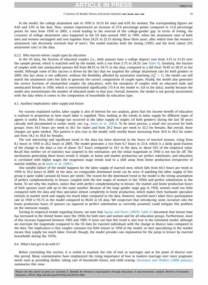
JID:YREDY AID:710 /FLA [m3G; v1.143-dev; Prn:17/12/2014; 13:01] P.19 (1-26)
F. Guvenen, M. Rendall / Review of Economic Dynamics ••• (••••) •••–••• 19
In the model, the college attainment rate in 1950 is 16.1% for men and 6.0% for women. The corresponding figures are 9.6% and 5.9% in the data. Thus, women experienced an increase of 27.4 percentage points compared to 13.0 percentage points for men from 1950 to 2005, a trend leading to the reversal of the college-gender gap. In terms of timing, the crossover of college attainment rates happened in the US data around 1993 to 1995, when the attainment rates of both men and women overlapped and rose together from 24.2% to 25.1% during these three years, after which time the women’s attainment rate decisively overtook that of men’s. The model matches both the timing (1995) and the level (about 25% attainment rate) in the data.
6.2.2. Who marries whom: couple types by educationIn the US data, the fraction of educated couples (i.e., both spouses have a college degree) rose from 3.1% to 21.5% over
the sample period, which is matched well by the model, with a rise from 2.7% to 24.3% (see Table 4). Similarly, the fraction of couples with two uneducated spouses fell from 88.5% to 59.7% in the data, compared to a fall from 78.4% to 58.1% in the model. Although some of this success is driven by the fact that we targeted the college attainment rate for both genders in 2005, this fact alone is not sufficient: without the flexibility afforded by assortative matching (θ11
m > 1), the model can still match the attainment rates but fails to generate the correct composition of couple types. Finally, the model also generates the correct fractions of mismatched couples (by education), with the exception of couples with an educated male and uneducated female in 1950, which is overestimated significantly (15.4 in the model vs. 6.8 in the data), mainly because the model also overestimates the number of educated males in that year. Overall, however, the model is not grossly inconsistent with the data when it comes to the composition of households by education type.
6.3. Auxiliary implications: labor supply and leisure
For reasons explained earlier, labor supply is also of interest for our analysis, given that the income benefit of education is realized in proportion to how much labor is supplied. Thus, looking at the trends in labor supply for different types of agents is useful. First, little change has occurred in the labor supply of singles (of both genders) during the last 50 years (already well documented in earlier work; see, e.g., Jones et al., 2003). To be more precise, a small rise occurred for both groups: from 34.5 hours per week to 36.1 for males and from 29.2 hours per week to 32.2 for females. But overall, these changes are quite modest. This pattern is also true in the model, with weekly hours increasing from 36.9 to 38.2 for males and from 34.2 to 36.8 for females.
The real interesting and significant trend in the data has been observed in the hours of married women, rising from 8.1 hours in 1950 to 26.2 hours in 2005. The model generates a rise from 6.7 hours to 23.4, which is a fairly good fraction of the change in the data—a rise of about 16.7 hours compared to 18.1 in the data, or about 92% of the empirical value. Recall that neither set of statistics was targeted in the estimation—yet the initial magnitude in 1950 is not too far off. The mechanism generating these hours trends is simple, as home and market production are prefect substitutes, and education is correlated with higher wages the exogenous wage trends lead to a shift away from home production irrespective of marital stability as in Jones et al. (2003).
One notable failure of the model happens for the labor supply of married men, which falls from 64.3 hours per week in 1950 to 39.2 hours in 2005. In the data, no comparable downward trend can be seen—if anything the labor supply of this group is quite stable (around 42 hours per week). The reason for the downward trend in the model is the strong assumption of perfect complementarity in leisure, coupled with the low wages of women in the 1950s and perfect substitution in the home. To see why this matters, notice that with perfect complementarity in leisure, the market and home production hours of both spouses must add up to the same number. Because of the large gender wage gap in 1950, women work too little compared with the data and thus specialize almost completely in home production, which makes their husbands specialize entirely in market work and supply too much labor compared to the data. However, married men’s labor force participation rate in 1950 is 93.7% in the model compared to 96.6% in US data. We conjecture that introducing some curvature into the home production hours of spouses (as opposed to perfect substitution as currently assumed) could mitigate this problem on the intensive margin.
Turning to empirical trends regarding leisure, we note that Aguiar and Hurst (2007b, Table V) document that leisure time has increased in the United States since the 1950s for both men and women and for all education groups. Furthermore, most of this increase happened between 1965 and 1985. It turns out that this trend is also true in the estimated model, although we overstate the magnitude compared to the US data for married individuals with the change in divorce laws compared to the data. The implication is that couples consume too little leisure in 1950 in the model, so men specializing in the market means they supply too much labor. Overall, though, the model provides one explanation for the jump in leisure by married households during the 1970s.
6.4. What’s love got to do with it?
Before concluding this section, it is useful to examine the role of love in marriages and at the point of divorce over this period. Many commentators have emphasized the rising importance of love in modern marriage over more pragmatic needs such as providing shelter, taking care of household chores, and child rearing. Stevenson and Wolfers (2008, January)summarize this view:
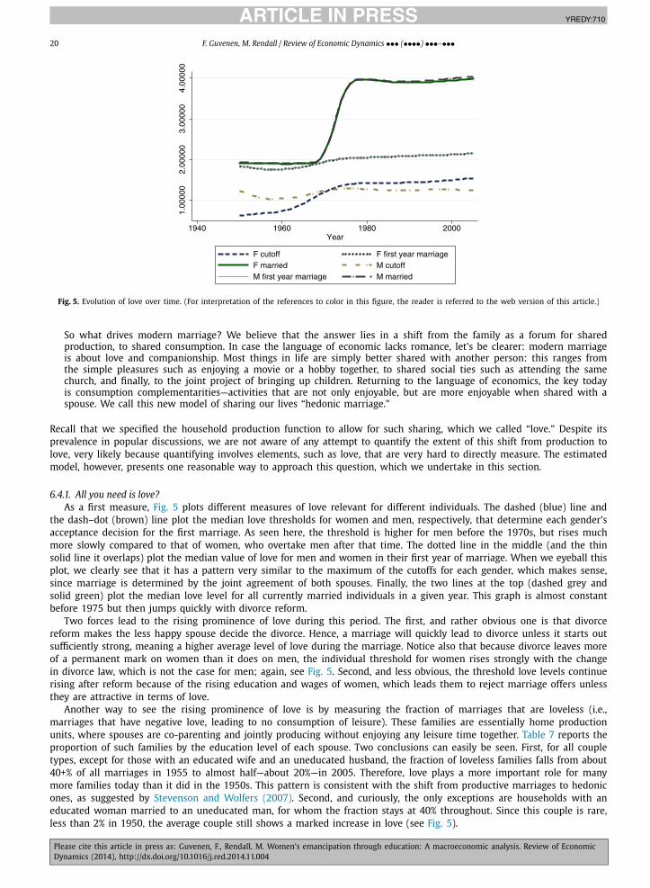
JID:YREDY AID:710 /FLA [m3G; v1.143-dev; Prn:17/12/2014; 13:01] P.20 (1-26)
20 F. Guvenen, M. Rendall / Review of Economic Dynamics ••• (••••) •••–•••
Fig. 5. Evolution of love over time. (For interpretation of the references to color in this figure, the reader is referred to the web version of this article.)
So what drives modern marriage? We believe that the answer lies in a shift from the family as a forum for shared production, to shared consumption. In case the language of economic lacks romance, let’s be clearer: modern marriage is about love and companionship. Most things in life are simply better shared with another person: this ranges from the simple pleasures such as enjoying a movie or a hobby together, to shared social ties such as attending the same church, and finally, to the joint project of bringing up children. Returning to the language of economics, the key today is consumption complementarities—activities that are not only enjoyable, but are more enjoyable when shared with a spouse. We call this new model of sharing our lives “hedonic marriage.”
Recall that we specified the household production function to allow for such sharing, which we called “love.” Despite its prevalence in popular discussions, we are not aware of any attempt to quantify the extent of this shift from production to love, very likely because quantifying involves elements, such as love, that are very hard to directly measure. The estimated model, however, presents one reasonable way to approach this question, which we undertake in this section.
6.4.1. All you need is love?As a first measure, Fig. 5 plots different measures of love relevant for different individuals. The dashed (blue) line and
the dash–dot (brown) line plot the median love thresholds for women and men, respectively, that determine each gender’s acceptance decision for the first marriage. As seen here, the threshold is higher for men before the 1970s, but rises much more slowly compared to that of women, who overtake men after that time. The dotted line in the middle (and the thin solid line it overlaps) plot the median value of love for men and women in their first year of marriage. When we eyeball this plot, we clearly see that it has a pattern very similar to the maximum of the cutoffs for each gender, which makes sense, since marriage is determined by the joint agreement of both spouses. Finally, the two lines at the top (dashed grey and solid green) plot the median love level for all currently married individuals in a given year. This graph is almost constant before 1975 but then jumps quickly with divorce reform.
Two forces lead to the rising prominence of love during this period. The first, and rather obvious one is that divorce reform makes the less happy spouse decide the divorce. Hence, a marriage will quickly lead to divorce unless it starts out sufficiently strong, meaning a higher average level of love during the marriage. Notice also that because divorce leaves more of a permanent mark on women than it does on men, the individual threshold for women rises strongly with the change in divorce law, which is not the case for men; again, see Fig. 5. Second, and less obvious, the threshold love levels continue rising after reform because of the rising education and wages of women, which leads them to reject marriage offers unless they are attractive in terms of love.
Another way to see the rising prominence of love is by measuring the fraction of marriages that are loveless (i.e., marriages that have negative love, leading to no consumption of leisure). These families are essentially home production units, where spouses are co-parenting and jointly producing without enjoying any leisure time together. Table 7 reports the proportion of such families by the education level of each spouse. Two conclusions can easily be seen. First, for all couple types, except for those with an educated wife and an uneducated husband, the fraction of loveless families falls from about 40+% of all marriages in 1955 to almost half—about 20%—in 2005. Therefore, love plays a more important role for many more families today than it did in the 1950s. This pattern is consistent with the shift from productive marriages to hedonic ones, as suggested by Stevenson and Wolfers (2007). Second, and curiously, the only exceptions are households with an educated woman married to an uneducated man, for whom the fraction stays at 40% throughout. Since this couple is rare, less than 2% in 1950, the average couple still shows a marked increase in love (see Fig. 5).
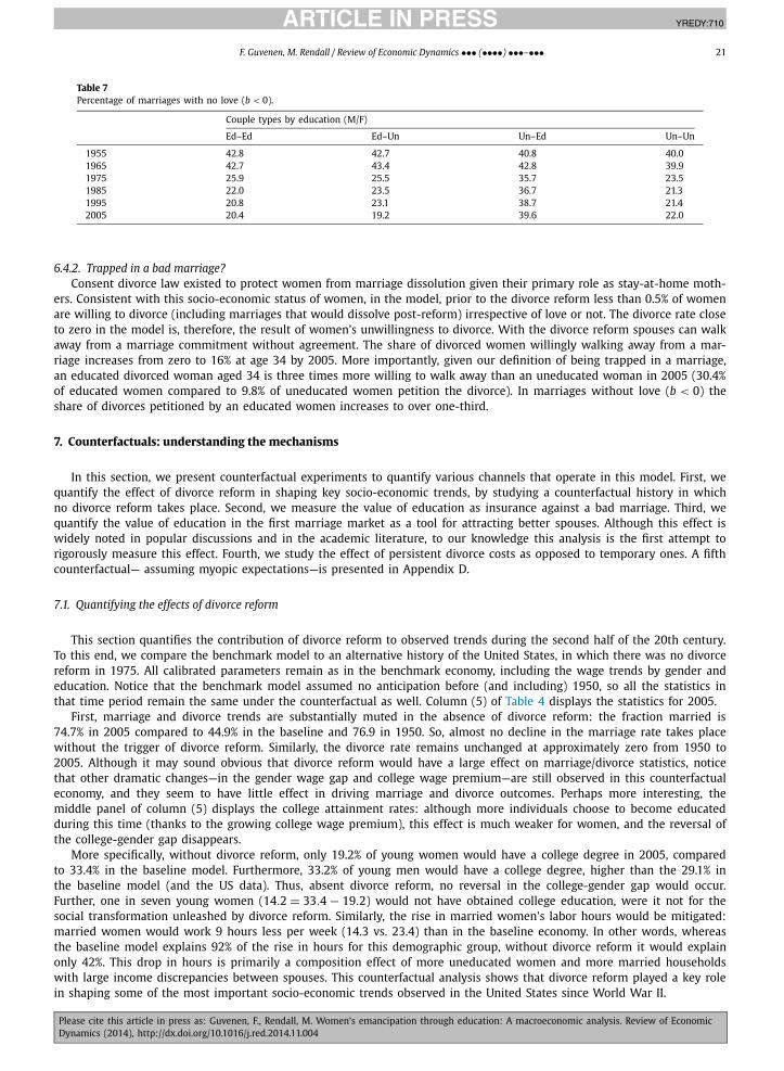
JID:YREDY AID:710 /FLA [m3G; v1.143-dev; Prn:17/12/2014; 13:01] P.21 (1-26)
F. Guvenen, M. Rendall / Review of Economic Dynamics ••• (••••) •••–••• 21
Table 7Percentage of marriages with no love (b < 0).
Couple types by education (M/F)
Ed–Ed Ed–Un Un–Ed Un–Un
1955 42.8 42.7 40.8 40.01965 42.7 43.4 42.8 39.91975 25.9 25.5 35.7 23.51985 22.0 23.5 36.7 21.31995 20.8 23.1 38.7 21.42005 20.4 19.2 39.6 22.0
6.4.2. Trapped in a bad marriage?Consent divorce law existed to protect women from marriage dissolution given their primary role as stay-at-home moth-
ers. Consistent with this socio-economic status of women, in the model, prior to the divorce reform less than 0.5% of women are willing to divorce (including marriages that would dissolve post-reform) irrespective of love or not. The divorce rate close to zero in the model is, therefore, the result of women’s unwillingness to divorce. With the divorce reform spouses can walk away from a marriage commitment without agreement. The share of divorced women willingly walking away from a mar-riage increases from zero to 16% at age 34 by 2005. More importantly, given our definition of being trapped in a marriage, an educated divorced woman aged 34 is three times more willing to walk away than an uneducated woman in 2005 (30.4% of educated women compared to 9.8% of uneducated women petition the divorce). In marriages without love (b < 0) the share of divorces petitioned by an educated women increases to over one-third.
7. Counterfactuals: understanding the mechanisms
In this section, we present counterfactual experiments to quantify various channels that operate in this model. First, we quantify the effect of divorce reform in shaping key socio-economic trends, by studying a counterfactual history in which no divorce reform takes place. Second, we measure the value of education as insurance against a bad marriage. Third, we quantify the value of education in the first marriage market as a tool for attracting better spouses. Although this effect is widely noted in popular discussions and in the academic literature, to our knowledge this analysis is the first attempt to rigorously measure this effect. Fourth, we study the effect of persistent divorce costs as opposed to temporary ones. A fifth counterfactual— assuming myopic expectations—is presented in Appendix D.
7.1. Quantifying the effects of divorce reform
This section quantifies the contribution of divorce reform to observed trends during the second half of the 20th century. To this end, we compare the benchmark model to an alternative history of the United States, in which there was no divorce reform in 1975. All calibrated parameters remain as in the benchmark economy, including the wage trends by gender and education. Notice that the benchmark model assumed no anticipation before (and including) 1950, so all the statistics in that time period remain the same under the counterfactual as well. Column (5) of Table 4 displays the statistics for 2005.
First, marriage and divorce trends are substantially muted in the absence of divorce reform: the fraction married is 74.7% in 2005 compared to 44.9% in the baseline and 76.9 in 1950. So, almost no decline in the marriage rate takes place without the trigger of divorce reform. Similarly, the divorce rate remains unchanged at approximately zero from 1950 to 2005. Although it may sound obvious that divorce reform would have a large effect on marriage/divorce statistics, notice that other dramatic changes—in the gender wage gap and college wage premium—are still observed in this counterfactual economy, and they seem to have little effect in driving marriage and divorce outcomes. Perhaps more interesting, the middle panel of column (5) displays the college attainment rates: although more individuals choose to become educated during this time (thanks to the growing college wage premium), this effect is much weaker for women, and the reversal of the college-gender gap disappears.
More specifically, without divorce reform, only 19.2% of young women would have a college degree in 2005, compared to 33.4% in the baseline model. Furthermore, 33.2% of young men would have a college degree, higher than the 29.1% in the baseline model (and the US data). Thus, absent divorce reform, no reversal in the college-gender gap would occur. Further, one in seven young women (14.2 = 33.4 − 19.2) would not have obtained college education, were it not for the social transformation unleashed by divorce reform. Similarly, the rise in married women’s labor hours would be mitigated: married women would work 9 hours less per week (14.3 vs. 23.4) than in the baseline economy. In other words, whereas the baseline model explains 92% of the rise in hours for this demographic group, without divorce reform it would explain only 42%. This drop in hours is primarily a composition effect of more uneducated women and more married households with large income discrepancies between spouses. This counterfactual analysis shows that divorce reform played a key role in shaping some of the most important socio-economic trends observed in the United States since World War II.
JID:YREDY AID:710 /FLA [m3G; v1.143-dev; Prn:17/12/2014; 13:01] P.22 (1-26)
22 F. Guvenen, M. Rendall / Review of Economic Dynamics ••• (••••) •••–•••
7.2. Education as insurance against a bad marriage
The story of Fraidy Reiss in the introduction provides one example in which education allowed a woman to improve her outside options and avoid being trapped in a bad marriage. In general, this outside option depends on the divorced individual’s wage as well as his/her opportunities in the remarriage market. In this section we quantify this insurance value of education. What if married women believed that a divorce would leave them with little income and worse re-marriage options? Would educated women stay longer in bad marriages? Would they search longer in the first marriage market?
These questions maybe answered by taking different approaches. Each approach sheds light on a different aspect of the problem. We proceed in three steps. We describe each experiment from a woman’s perspective, with the understanding that each experiment is also conducted symmetrically for men. Furthermore, we conduct the experiments for women in the 10th, 50th (median), and 90th percentiles of the ability distribution and for cohorts who turn age 20 before and after 1975 separately. To convert the welfare effect into easily understandable terms, we ask how much each hypothetical woman would need to be compensated in units of leisure hours at every date and state so as to be indifferent between the baseline economy and each counterfactual economy.
Experiment 1. First, suppose that all individuals make their first marriage decisions as in the benchmark model. Upon marriage, however, each educated woman comes to believe that if she were to divorce, her future path would be the same as an uneducated woman (with the corresponding value function and a wage that corresponds to her actual ability percentile but drawn from the wage distribution of uneducated women). In this first counterfactual, we assume that these beliefs are incorrect and that if these educated women were to actually divorce, their subsequent lives would be the same as educated women (with the correct wage and remarriage probability). We make this assumption because we simply want to measure the effect of this fear factor.
Under this scenario, we find that educated women are more likely to be trapped (to spend a longer duration in a bad marriage) when their ability is higher: for women in the 90th percentile, the average length of the first marriage would increase from 26.4 years to 29.2 for the post-1975 cohorts, and from 30.2 to 31.6 for earlier cohorts. Moreover, fewer of these first marriages now end in divorce, declining from 78% to 76% in the model. However, for women in the 10th percentile of the ability distribution, there is virtually no effect on the length of marriages or divorce probabilities. Clearly, this is because after divorce reform, there is no protection from an involuntary divorce, therefore, even though these low-wage women may not want to divorce, their husbands still will.
Experiment 2. A second version of this experiment assumes that upon divorce educated women actually face the same prospects as uneducated women (so, not only expectations but also actual paths are changed). Perhaps unsurprisingly, edu-cated women are now trapped in worse marriages for longer durations and spend more years as divorced individuals with low incomes. Specifically, women in the 90th percentile in the post-1975 cohorts spend 15.0 years as divorced individuals, compared with 9.9 years in the benchmark model, and the fraction remarried drops from 81% to 51%. Similarly, women at the median spend 17.2 years as divorced individuals (compared with 13.0), and the fraction remarried drops from 68% to 46%. Again, the effect is smallest for women at the 10th percentile, where years divorced increase from 16.0 to 17.6 and the fraction remarried drops from 55% to 46%. In contrast, for men in this same scenario, the years spent as divorced individuals actually decrease. This is because men do not suffer from a permanent loss of economies of scale upon divorce (although they still face less efficient matching). Welfare losses from this counterfactual are highest (70% of baseline leisure hours) for women in the 90th percentile for the post-1975 cohorts.
Experiment 3 (preferred counterfactual). The previous two experiments assumed that women were completely oblivious to the cost of divorce until after entering a marriage—an assumption leading to potentially large welfare losses. A third experiment now allows women to correctly anticipate their future expectations before entering their first marriage. Welfare losses are still quite large. We view this experiment as the most complete of the three and report the full results in the top panel of Table 8. Comparing columns (1) and (3), it becomes clear that the welfare benefits are much larger for women than for men in the post-1975 cohorts at low ability levels, but the gap closes as we go up the ability scale or consider earlier cohorts (or both). Therefore, consistent with our hypothesis, education is a better insurance against divorce especially for low-ability women, and it has become even more important over time.
In addition to the large welfare effects, women remain married longer than before (30.1 vs. 26.3 years) and spend a longer time as divorced individuals (12.2 years for women in the 90th percentile after 1975). Women also wait to marry longer, with the average age at first marriage increasing from 24.3 to 26.4. In contrast, men marry slightly sooner (at 23.8 in the benchmark compared to 22.6 here). What were women waiting for? A higher love draw, that is, a healthier marriage. Nonetheless, although initial love is higher, average love at the date of separation is lower in the counterfactual compared to the benchmark. Even though women would wait for a better match, they still spend more time in a worse marriage. The large welfare losses for men, especially in the 90th percentile, are explained not by a larger cost in the marriage market but by the larger college premium for men than for women.

JID:YREDY AID:710 /FLA [m3G; v1.143-dev; Prn:17/12/2014; 13:01] P.23 (1-26)
F. Guvenen, M. Rendall / Review of Economic Dynamics ••• (••••) •••–••• 23
Table 8Welfare benefits of education in the marriage market.
Cohorts Wage percentile Women Men
% hours $ % hours $(1) (2) (3) (4)
Being trapped in a marriagePre-1975 P10 25.6 3031 15.9 4804
P50 30.9 5036 20.3 8436P90 30.2 6760 22.2 12 667
Post-1975 P10 40.0 7288 16.2 4890P50 43.8 10 912 24.7 10 238P90 40.1 13 779 32.2 18 370
Attracting better spousePre-1975 P10 13.5 1594 10.2 3065
P50 13.7 2231 9.8 4055P90 12.3 2750 9.2 5271
Post-1975 P10 18.2 3323 9.1 2738P50 18.5 4604 11.2 4629P90 17.4 5995 11.4 6503
Notes: Columns (1) and (3) express the welfare benefit in terms of leisure hours divided by the average market hours of the applicable gender averaged across all ability levels. For example, in the first column, last row of the top panel, the benefit is equal to 40% of average market hours of women in the post-1975 cohorts. The $ column reports the corresponding dollar value (with year 2000 as basis), by evaluating the hours at the corresponding hourly wage for that percentile, assuming a full-year (52 weeks) worker.
7.3. How effective is education for attracting better spouses?
It is often remarked that education is an effective tool for meeting and attracting educated spouses (e.g., Chiappori et al., 2009). The model features two channels through which this effect could work: (i) assortative meeting and (ii) higher wages that attract better spouses, especially when women participate in the labor force.
To quantify this potential benefit, we conduct the following thought experiment. Suppose that an educated woman was unable to experience the marriage market benefit, which we think of as follows: (i) an educated woman meets educated men at the rate of an uneducated single woman (e.g., her meeting probability is computed with θ10
m instead of θ11m ), and
(ii) when a man meets this woman, he will view her as an uneducated woman (with a wage that is in the same percentile distribution of her true wage, but drawn from the uneducated females’ wage distribution). We assume that this incorrect perception is limited to the first marriage market and disappears afterward. In reality, the woman will still receive her actual educated wage throughout her life and choose her labor supply accordingly. Moreover, once she does marry, the husband will find out the true type of his wife, and labor supply and subsequent divorce decisions (if any) will be determined ac-cordingly. Therefore, this experiment intends to isolate the benefit of education solely as a device for (potentially) attracting a better spouse. We repeat the same experiment for males.
The bottom panel of Table 8 displays the results. As seen here, the welfare benefits are not as large, ranging from about one-third to one-half of the benefits of the insurance value of education. Again, the benefits are also higher for women compared with men, increase over time, and they do vary noticeably with the ability level of individuals.
7.4. Alternative formulations
7.4.1. Matching the fraction divorced in 1950 (the MFD model)One notable drawback of the benchmark model is that it fails to generate divorces in the earlier part of the sample. One
question this raises is: What if we directly target the fraction of individuals who are divorced in 1950 in our estimation, instead of the fraction who are single (as done above)? This exercise gives a useful idea about the trade-offs inherent in the model.
Columns (3) and (4) in Table 9 report the results. Although this change allows the model to match the fraction of individuals that are divorced in 1950 (3%) and thus also nicely match the rise in divorces over time, it also fails to generate any decline in the marriage rate and a rise in the fraction of individuals that are single. These are key failings in our view, since these latter two trends are central to our purposes. Apart from these failings, however, this alternative model continues to generate the reversal of the college-gender gap and the rise in labor supply for married women (although the magnitudes of both are quite a bit smaller than in the benchmark model). Overall, we conclude that forcing the model to match the high divorce rate in the 1950s stretches the model’s abilities and yields an overall degradation in its performance.34
34 Another way of generating high divorce in 1950 would be to allow “transferable utility” between spouses, in the spirit of the Coase theorem (see also footnote 10). In the model, prior to 1975 men are more likely to desire a divorce (given the high childcare cost and low wages of divorced women), but given consent divorce they are unable to do so. In a less restrictive scenario, one could imagine husbands transferring utility to their wives in order to
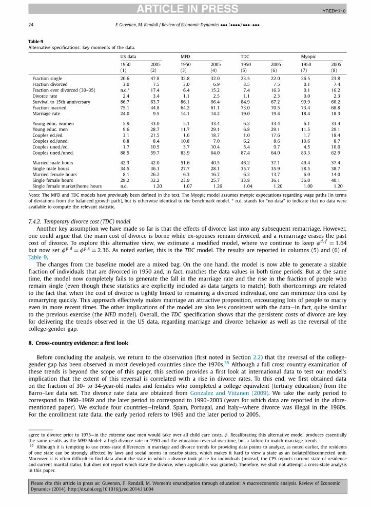
JID:YREDY AID:710 /FLA [m3G; v1.143-dev; Prn:17/12/2014; 13:01] P.24 (1-26)
24 F. Guvenen, M. Rendall / Review of Economic Dynamics ••• (••••) •••–•••
Table 9Alternative specifications: key moments of the data.
US data MFD TDC Myopic
1950 2005 1950 2005 1950 2005 1950 2005(1) (2) (3) (4) (5) (6) (7) (8)
Fraction single 20.6 47.8 32.8 32.0 23.5 22.0 26.5 23.8Fraction divorced 3.0 7.5 3.0 6.9 3.5 7.5 0.1 7.4Fraction ever divorced (30–35) n.d.∗ 17.4 6.4 15.2 7.4 16.3 0.1 16.2Divorce rate 2.4 3.4 1.1 2.5 1.1 2.3 0.0 2.3Survival to 15th anniversary 86.7 63.7 86.1 66.4 84.9 67.2 99.9 66.2Fraction married 75.1 44.8 64.2 61.1 73.0 70.5 73.4 68.8Marriage rate 24.0 9.5 14.1 14.2 19.0 19.4 18.4 18.3
Young educ. women 5.9 33.0 5.1 33.4 6.2 33.4 6.1 33.4Young educ. men 9.6 28.7 11.7 29.1 6.8 29.1 11.5 29.1Couples ed./ed. 3.1 21.5 1.6 18.7 1.0 17.6 1.7 18.4Couples ed./uned. 6.8 8.4 10.8 7.0 6.2 8.6 10.6 8.7Couples uned./ed. 1.7 10.5 3.7 10.4 5.4 9.7 4.5 10.0Couples uned./uned. 88.5 59.7 83.9 64.0 87.4 64.0 83.3 62.9
Married male hours 42.3 42.0 51.6 40.5 46.2 37.1 49.4 37.4Single male hours 34.5 36.1 27.7 28.1 35.7 35.9 38.5 38.7Married female hours 8.1 26.2 6.3 16.7 6.2 13.7 6.0 14.0Single female hours 29.2 32.2 23.9 25.7 33.8 36.1 36.0 40.1Single female market/home hours n.d. 1.20 1.07 1.26 1.04 1.20 1.00 1.20
Notes: The MFD and TDC models have previously been defined in the text. The Myopic model assumes myopic expectations regarding wage paths (in terms of deviations from the balanced growth path), but is otherwise identical to the benchmark model. ∗ n.d. stands for “no data” to indicate that no data were available to compute the relevant statistic.
7.4.2. Temporary divorce cost (TDC) modelAnother key assumption we have made so far is that the effects of divorce last into any subsequent remarriage. However,
one could argue that the main cost of divorce is borne while ex-spouses remain divorced, and a remarriage erases the past cost of divorce. To explore this alternative view, we estimate a modified model, where we continue to keep φd, f = 1.64but now set φp,d = φp,s = 2.36. As noted earlier, this is the TDC model. The results are reported in columns (5) and (6) of Table 9.
The changes from the baseline model are a mixed bag. On the one hand, the model is now able to generate a sizable fraction of individuals that are divorced in 1950 and, in fact, matches the data values in both time periods. But at the same time, the model now completely fails to generate the fall in the marriage rate and the rise in the fraction of people who remain single (even though these statistics are explicitly included as data targets to match). Both shortcomings are related to the fact that when the cost of divorce is tightly linked to remaining a divorced individual, one can minimize this cost by remarrying quickly. This approach effectively makes marriage an attractive proposition, encouraging lots of people to marry even in more recent times. The other implications of the model are also less consistent with the data—in fact, quite similar to the previous exercise (the MFD model). Overall, the TDC specification shows that the persistent costs of divorce are key for delivering the trends observed in the US data, regarding marriage and divorce behavior as well as the reversal of the college-gender gap.
8. Cross-country evidence: a first look
Before concluding the analysis, we return to the observation (first noted in Section 2.2) that the reversal of the college-gender gap has been observed in most developed countries since the 1970s.35 Although a full cross-country examination of these trends is beyond the scope of this paper, this section provides a first look at international data to test our model’s implication that the extent of this reversal is correlated with a rise in divorce rates. To this end, we first obtained data on the fraction of 30- to 34-year-old males and females who completed a college equivalent (tertiary education) from the Barro–Lee data set. The divorce rate data are obtained from Gonzalez and Viitanen (2009). We take the early period to correspond to 1960–1969 and the later period to correspond to 1990–2003 (years for which data are reported in the afore-mentioned paper). We exclude four countries—Ireland, Spain, Portugal, and Italy—where divorce was illegal in the 1960s. For the enrollment rate data, the early period refers to 1965 and the later period to 2005.
agree to divorce prior to 1975—in the extreme case men would take over all child care costs, φ. Recalibrating this alternative model produces essentially the same results as the MFD Model: a high divorce rate in 1950 and the education reversal overtime, but a failure to match marriage trends.35 Although it is tempting to use cross-state differences in marriage and divorce trends for providing data points to analyze, as noted earlier, the residents
of one state can be strongly affected by laws and social norms in nearby states, which makes it hard to view a state as an isolated/disconnected unit. Moreover, it is often difficult to find data about the state in which a divorce took place for individuals (instead, the CPS reports current state of residence and current marital status, but does not report which state the divorce, when applicable, was granted). Therefore, we shall not attempt a cross-state analysis in this paper.

JID:YREDY AID:710 /FLA [m3G; v1.143-dev; Prn:17/12/2014; 13:01] P.25 (1-26)
F. Guvenen, M. Rendall / Review of Economic Dynamics ••• (••••) •••–••• 25
Fig. 6. Cross-country data: change in divorce rates vs. change in college-gender gap.
First, we compute the cross-sectional correlation of divorce rates and female college attainment rates. In this sample of 12 countries, the correlation is 0.57. Second, and more important, we examine the change in divorce rates over this period and how it is related to the change in female attainment rates. The correlation is 0.49. Third, to examine the specific prediction of our model, we compute the cross-country correlation between the change in the college-gender gap (male/female college attainment rate) and the change in the divorce rate. This correlation is 0.51. Fig. 6 plots the data for each country in the sample. Except for Iceland and Finland, the remaining 10 countries line up nicely along the regression line. Although preliminary, this evidence suggests that socio-economic trends involving divorce rates could be an important component for understanding male versus female college attainment rates over time.
9. Conclusion
This paper studied the role of education as insurance against a bad marriage, against the backdrop of some prominent socio-economic trends since the 1950s. The estimated structural model shows that the interaction of divorce reform with asymmetric costs of divorce can explain both the timing and the magnitude of the reversal of the college-gender gap. This interaction also seems essential for generating the large magnitudes of some other trends—such as the large decline in the marriage rate and the substantial rise in the divorce rate, as well as the large rise in employment for married women.
The estimated model also allowed us to quantify the insurance value of education upon divorce. For women, the value of education for preventing being trapped in a marriage is very large, is significantly higher for younger cohorts (born after 1975), and rises with women’s ability level. The same general pattern also holds for men, with a somewhat smaller magnitude. The corresponding dollar values are substantial, ranging from $7000 to $11 600 per annum for median women and as high as $15 000 for high-ability women (in the 90th percentile). It is even higher for men in dollar terms, given their higher wage rates. The value of education for attracting a better spouse is also higher for more recent cohorts and higher for women than for men. To our knowledge, our paper is the first to empirically quantify both of these welfare effects.
In keeping with the existing literature, one assumption we maintained in this paper is that divorce reform was exogenous with respect to the model. However, given the central role our analysis attributes to the reform, thinking about how this assumption might be relaxed is a useful step. In ongoing work, we explore the thesis that the divorce reform itself can be generated endogenously in a framework similar to the one studied here but in which a social planner is maximizing a utilitarian objective, by choosing (every period) between the consent and unilateral regimes. As the gender wage gap starts to close and divorce rates start to rise slowly, the welfare loss from individuals stuck in marriages under the consent regime grows to the point where switching to the unilateral regime becomes optimal. The social planner then adopts the reform, which in turn triggers much larger changes in divorce rates as observed in the US data. Although preliminary, we believe this work provides a sensible first step to acknowledging that laws also change for a reason—typically, in response to societal demands.
An interesting extension of the current model would be the introduction of intra-household bargaining. How this ex-tension would affect our results is less obvious than it might first appear for two reasons. First, bargaining would provide a margin through which spouses can compensate each other in response to changing outside options, tending to reduce the divorce rate. However, such a model would have to be recalibrated to match the same targets, including the divorce

JID:YREDY AID:710 /FLA [m3G; v1.143-dev; Prn:17/12/2014; 13:01] P.26 (1-26)
26 F. Guvenen, M. Rendall / Review of Economic Dynamics ••• (••••) •••–•••
rate in the 2000s. Thus, it is not immediate that this alternative formulation would imply lower returns to education for women or a smaller effect of the divorce reform. Second, one of the main results of the paper is that the divorce reform has a large impact on women’s educational attainment. This may still largely be the case, because, with bargaining, educated women would get a larger share of the marriage surplus relative to uneducated women, which would increase the returns to education and, therefore, lead to higher educational attainment for women.
Appendix A. Supplementary material
Supplementary material related to this article can be found online at http://dx.doi.org/10.1016/j.red.2014.11.004.
References
Aguiar, M., Hurst, E., 2007a. Life-cycle prices and production. The American Economic Review 97 (5), 1533–1559.Aguiar, M., Hurst, E., 2007b. Measuring trends in leisure: the allocation of time over five decades. The Quarterly Journal of Economics 122 (3), 969–1006.Aiyagari, S.R., Greenwood, J., Guner, N., 2000. On the State of the Union. Journal of Political Economy 108 (2), 213–244.Altonji, J.G., Segal, L.M., 1996. Small-sample bias in GMM estimation of covariance structures. Journal of Business & Economic Statistics 14 (3), 353–366.Bahr, S.J., 1983. Marital dissolution laws: impact of recent changes for women. Journal of Family Issues 4 (3), 455–466.Becker, G.S., 1981. A Treatise on the Family. Harvard University Press, Cambridge, MA.Becker, G.S., 1994. Human Capital: A Theoretical and Empirical Analysis with Special Reference to Education, 3rd edition. National Bureau of Economic
Research, Inc. Number beck94-1 in NBER books.Blake, N.M., 1962. The Road to Reno: A History of Divorce in the United States. Macmillan, New York, NY.Caucutt, E.M., Guner, N., Knowles, J., 2002. Why do women wait? Matching, wage inequality, and the incentives for fertility delay. Review of Economic
Dynamics 5 (4), 815–855.Chade, H., Ventura, G., 2002. Taxes and marriage: a two-sided search analysis. International Economic Review 43 (3), 955–986.Chiappori, P.-A., Iyigun, M., Weiss, Y., 2008. Public goods, transferable utility and divorce laws. Working paper. Columbia University.Chiappori, P.-A., Iyigun, M., Weiss, Y., 2009. Investment in schooling and the marriage market. The American Economic Review 99 (5), 1689–1713.Cubeddu, L., Ríos-Rull, J.-V., 2003. Families as shocks. Journal of the European Economic Association 1 (2–3), 671–682.Elliott, D.B., Krivickas, K., Brault, M.W., Kreider, R.M., 2012. Historical marriage trends from 1890–2010: a focus on race differences. SEHSD Working Paper
2012-12.Fernandez, R., Wong, J.C., 2014. Free to leave? A welfare analysis of divorce regimes. NBER Working Papers 20251. National Bureau of Economic Research,
Inc.Freed, D.J., Foster Jr., H.H., 1969. Divorce American style. The Annals of the American Academy of Political and Social Science 383, 71–88.Freed, D.J., Foster Jr., H.H., 1981. Divorce in the fifty states: an overview. Family Law Quarterly 14 (4), 229–283.Gallipoli, G., Meghir, C., Violante, G.L., 2010. Equilibrium effects of education policies: a quantitative evaluation. Working paper. New York University.Goldin, C., Katz, L.F., Kuziemko, I., 2006. The homecoming of American college women: the reversal of the college gender gap. The Journal of Economic
Perspectives 20 (4), 133–156.Gonzalez, L., Viitanen, T.K., 2009. The effect of divorce laws on divorce rates in Europe. European Economic Review 53 (2), 127–138.Greenwood, J., Guner, N., Kocharkov, G., Santos, C., 2012. Technology and the changing family: a unified model of marriage, divorce, educational attainment
and married female labor-force participation. NBER Working Papers 17735. National Bureau of Economic Research, Inc.Heathcote, J., Storesletten, K., Violante, G.L., 2010. The macroeconomic implications of rising wage inequality in the United States. Journal of Political
Economy 118 (4), 681–722.Isen, A., Stevenson, B., 2010. Women’s education and family behavior: trends in marriage, divorce and fertility. In: Demography and the Economy, NBER
Chapters. National Bureau of Economic Research, Inc., pp. 107–140.Iyigun, M., Walsh, R.P., 2007. Endogenous gender power, household labor supply and the demographic transition. Journal of Development Economics 82 (1),
138–155.Jacob, H., 1988. Silent Revolution: The Transformation of Divorce Law in the United States. University of Chicago Press.Jacobson, P.H., 1959. American Marriage and Divorce. Rinehart, New York, NY.Jones, L.E., Manuelli, R.E., McGrattan, E.R., 2003. Why are married women working so much? Staff report 317. Federal Reserve Bank of Minneapolis.Knowles, J., 2013. Why are married men working so much? An aggregate analysis of intra-household bargaining and labor supply. Review of Economic
Studies 80 (3), 1055–1085.Kreider, R.M., Remarriage in the United States. Poster presented at the Annual Meeting of the American Sociological Association, Montreal, August 10–14,
2006.Kreider, R.M., Ellis, R., 2011. Number, timing, and duration of marriages and divorces: 2009. Current Population Reports P70-125. US Census Bureau.Marcassa, S., 2009. Divorce laws and divorce rate in the U.S. PSE Working Paper 2009-52.Mazzocco, M., Ruiz, C., Yamaguchi, S., 2013. Labor supply, wealth dynamics, and marriage decisions. Working paper. UCLA.Stevenson, B., Wolfers, J., 2007. Marriage and divorce: changes and their driving forces. The Journal of Economic Perspectives 21 (2), 27–52.Stevenson, B., Wolfers, J., 2008, January. Marriage and the market. Cato Unbound Online.Voena, A., 2012. Yours, mine and ours: do divorce laws affect the intertemporal behavior of married couples? SIEPR Discussion Paper 10-022.Wolfers, J., 2006. Did unilateral divorce laws raise divorce rates? A reconciliation and new results. The American Economic Review 96 (5), 1802–1820.