wolfgang huber dkfz heidelberg - bioconductor · local background estimation by morphological...
TRANSCRIPT

Error models and normalization
Wolfgang Huber
DKFZ Heidelberg

AcknowledgementsAnja von Heydebreck, Martin Vingron
Andreas Buness, Markus Ruschhaupt, Klaus Steiner, Jörg Schneider, Katharina Finis, Anke Schroth, Friederike Wilmer, Judith Boer, Holger Sültmann, Annemarie Poustka
Sandrine Dudoit, Robert Gentleman, Rafael Irizarry and Yee Hwa Yang: Bioconductor short course, summer 2002
and many others

4x4, 8x4, or 12x 4 sectors
17...38 rows and columns per sector
ca. 4000…46000probes/array
sector: corresponds to one print-tip
A microarray slide (spotted)Slide: 25x75 mm
Spot-to-spot: ca. 150-350 µm

Affymetrix oligonucleotide chips
25Oligonucleotide length
11No. probe pairs per target sequence
600,000No. probes11µmFeature size
hgU133plus2.0

Agilent oligonucleotide chips
60Oligonucleotide length44,000No. probes≈100µmFeature size
whole human genome kit (5/2004)

Terminologysample: RNA (cDNA) hybridized to the array, aka
target, mobile substrate.probe: DNA spotted on the array, aka spot,
immobile substrate.sector: rectangular matrix of spots printed using
the same print-tip (or pin), aka print-tip-groupplate: set of 384 (768) spots printed with DNA
from the same microtitre plate of clonesslide, arraychannel: data from one color (Cy3 = cyanine 3 =
green, Cy5 = cyanine 5 = red).batch: collection of microarrays with the same
probe layout.
Image Analysisscanner signal
resolution:5 or 10 mm spatial, 16 bit (65536) dynamical per channel
ca. 30-50 pixels per probe (60 µm spot size)40 MB per array

Image Analysisscanner signal
resolution:5 or 10 mm spatial, 16 bit (65536) dynamical per channel
ca. 30-50 pixels per probe (60 µm spot size)40 MB per array
Image Analysis

Image Analysisscanner signal
resolution:5 or 10 mm spatial, 16 bit (65536) dynamical per channel
ca. 30-50 pixels per probe (60 µm spot size)40 MB per array
Image Analysis
spot intensities2 numbers per probe (~100-300 kB)… auxiliaries: background, area, std dev, …

Image analysis1. Addressing. Estimate location of spot centers.

Image analysis1. Addressing. Estimate location of spot centers.
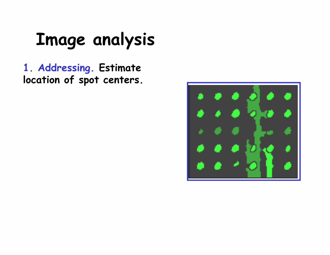
Image analysis1. Addressing. Estimate location of spot centers.

Image analysis
2. Segmentation. Classify pixels as foreground (signal) or background.
1. Addressing. Estimate location of spot centers.
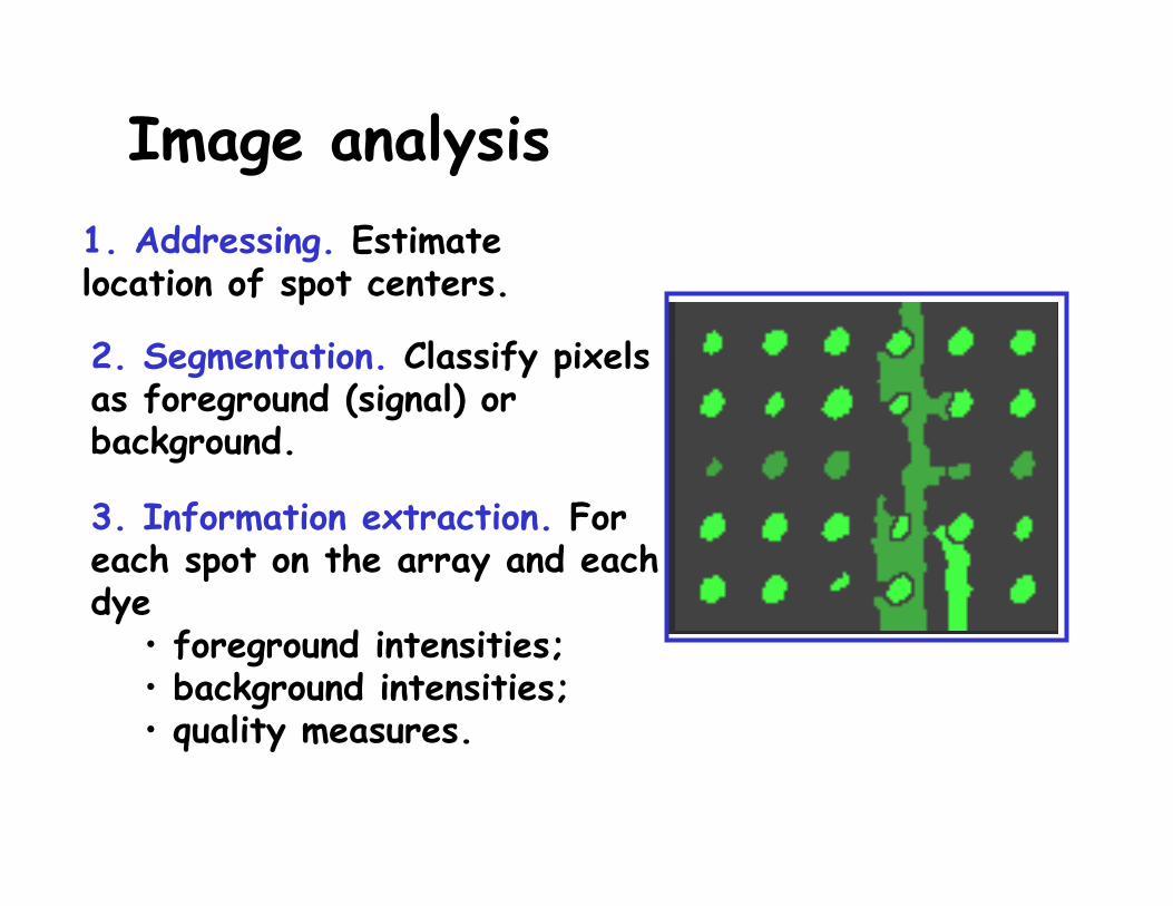
Image analysis
2. Segmentation. Classify pixels as foreground (signal) or background.
3. Information extraction. For each spot on the array and each dye
• foreground intensities;• background intensities; • quality measures.
1. Addressing. Estimate location of spot centers.

Image analysis
2. Segmentation. Classify pixels as foreground (signal) or background.
3. Information extraction. For each spot on the array and each dye
• foreground intensities;• background intensities; • quality measures.
R and G for each spot on the array.
1. Addressing. Estimate location of spot centers.
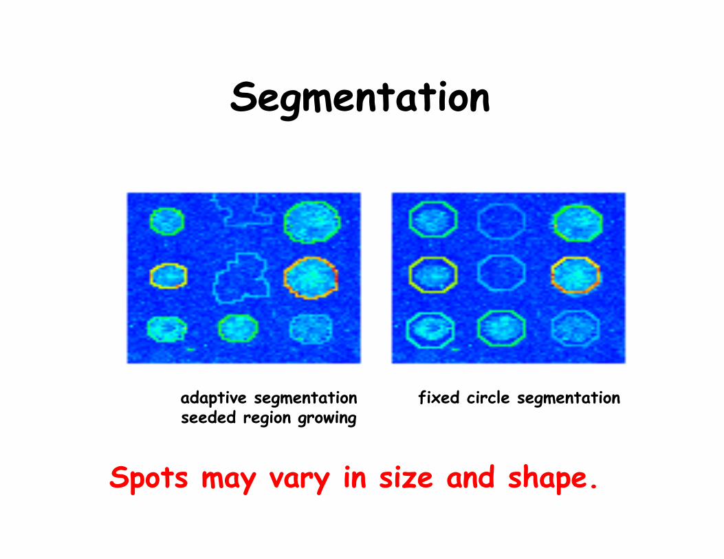
Segmentation
adaptive segmentationseeded region growing
fixed circle segmentation
Spots may vary in size and shape.

Local background
---- GenePix
---- QuantArray
---- ScanAlyze
Local background estimation by morphological opening
Image is probed with a window (aka structuring element), eg, a square with side length about twice the spot-to-spot distance.
Local background estimation by morphological opening
Image is probed with a window (aka structuring element), eg, a square with side length about twice the spot-to-spot distance.
Erosion: at each pixel, replace its value by the minimum value in the window around it.
Local background estimation by morphological opening
Image is probed with a window (aka structuring element), eg, a square with side length about twice the spot-to-spot distance.
Erosion: at each pixel, replace its value by the minimum value in the window around it.
Dilation: same with maximum
followed by
Do this separately for red and green images. This 'smoothes away' all structures that are smaller than the window
⇒ Image of the estimated background
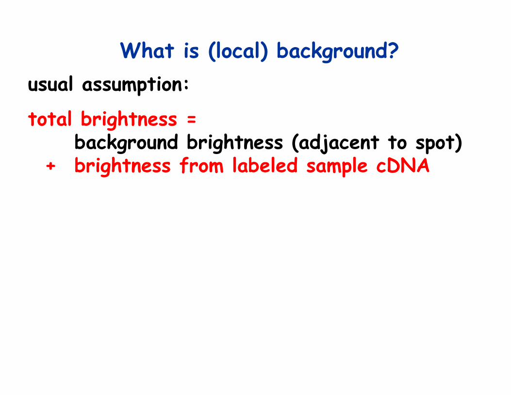
What is (local) background? usual assumption:
total brightness = background brightness (adjacent to spot)
+ brightness from labeled sample cDNA

What is (local) background? usual assumption:
total brightness = background brightness (adjacent to spot)
+ brightness from labeled sample cDNA

Affymetrix filesMain software from Affymetrix:
MAS - MicroArray Suite.DAT file: Image file, ~10^7 pixels, ~50 MB.
CEL file: probe intensities, ~500,000 numbers
CDF file: Chip Description File. Describes which probes go in which probe sets (genes, gene fragments, ESTs).

Image analysisDAT image files CEL filesEach probe cell: 10x10 pixels.Gridding: estimate location of probe cell
centers.Signal:
– Remove outer 36 pixels 8x8 pixels.– The probe cell signal, PM or MM, is the 75th percentile of the 8x8 pixel values.
Background: Average of the lowest 2% probe cells is taken as the background value and subtracted.
Compute also quality values.
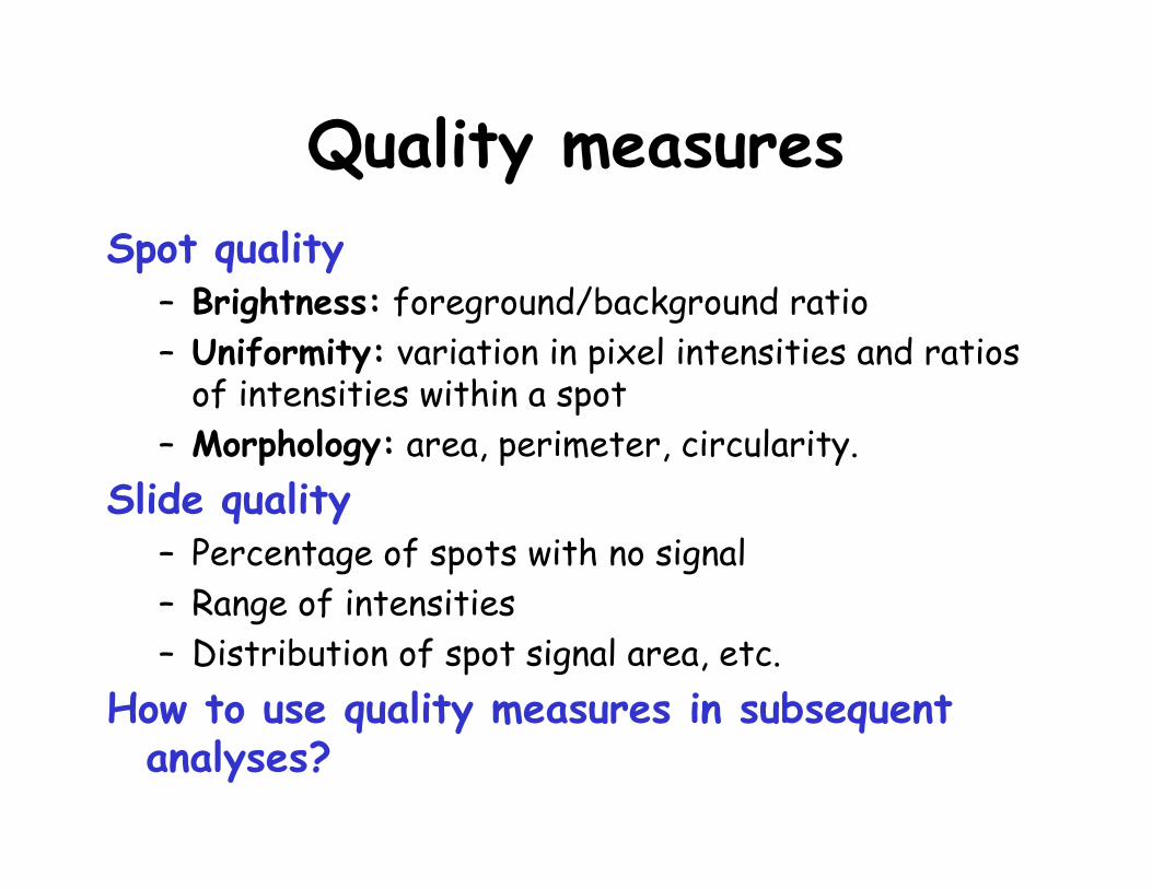
Quality measuresSpot quality
– Brightness: foreground/background ratio– Uniformity: variation in pixel intensities and ratios
of intensities within a spot– Morphology: area, perimeter, circularity.
Slide quality– Percentage of spots with no signal– Range of intensities– Distribution of spot signal area, etc.
How to use quality measures in subsequent analyses?

spot intensity dataspot intensity data
two-color spotted arrays
Prob
es (ge
nes)
n one-color arrays (Affymetrix, nylon)
conditions (samples)
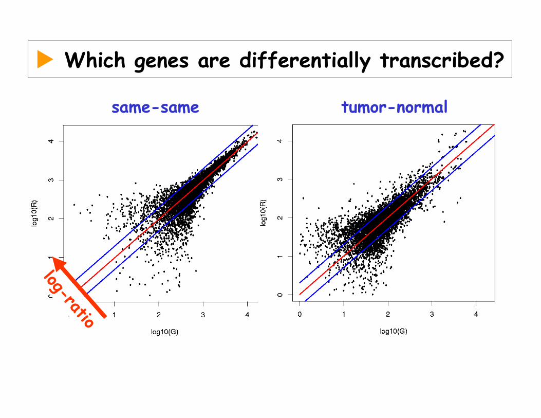
Which genes are differentially transcribed?
same-same tumor-normal
log-ratio

ratios and fold changesFold changes are useful to describe continuous changes in expression
10001500
3000x3
x1.5
A B C
0200
3000?
?
A B C
But what if the gene is “off” (below detection limit) in one condition?

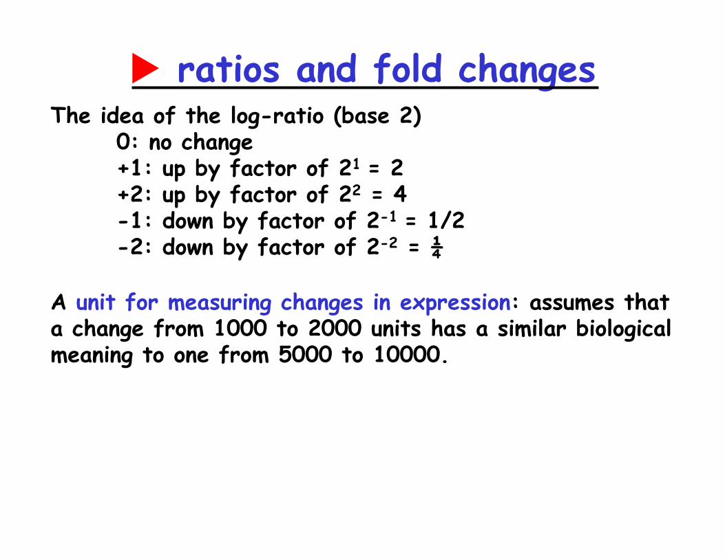
ratios and fold changesThe idea of the log-ratio (base 2)
0: no change+1: up by factor of 21 = 2+2: up by factor of 22 = 4-1: down by factor of 2-1 = 1/2-2: down by factor of 2-2 = ¼
ratios and fold changesThe idea of the log-ratio (base 2)
0: no change+1: up by factor of 21 = 2+2: up by factor of 22 = 4-1: down by factor of 2-1 = 1/2-2: down by factor of 2-2 = ¼
A unit for measuring changes in expression: assumes that a change from 1000 to 2000 units has a similar biological meaning to one from 5000 to 10000.
What about a change from 0 to 500?- conceptually- noise, measurement precision
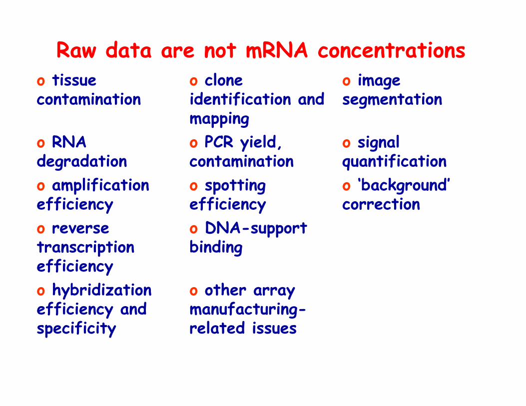
Raw data are not mRNA concentrations
o other array manufacturing-related issues
o hybridization efficiency and specificity
o DNA-support binding
o reverse transcription efficiency
o ‘background’ correction
o spotting efficiency
o amplification efficiency
o signal quantification
o PCR yield, contamination
o RNA degradation
o image segmentation
o clone identification and mapping
o tissue contamination
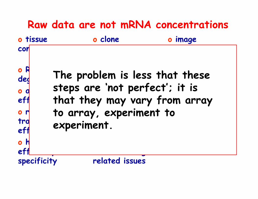
The problem is less that these steps are ‘not perfect’; it is that they may vary from array to array, experiment to experiment.
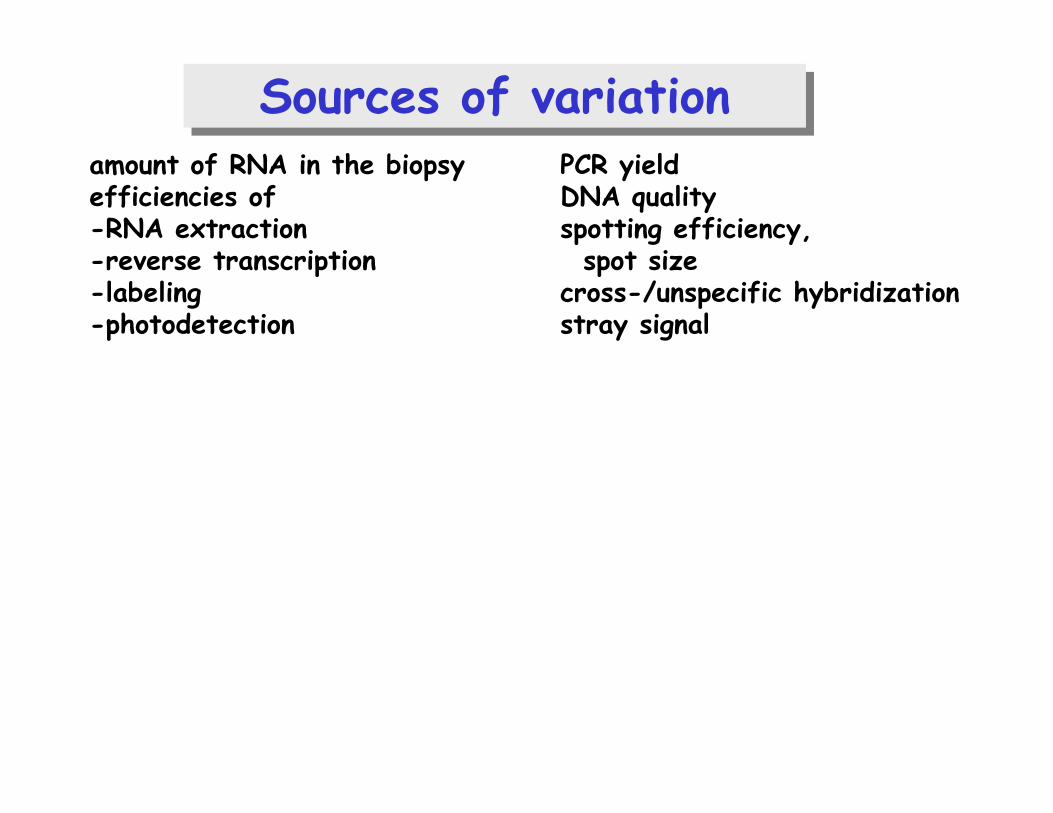
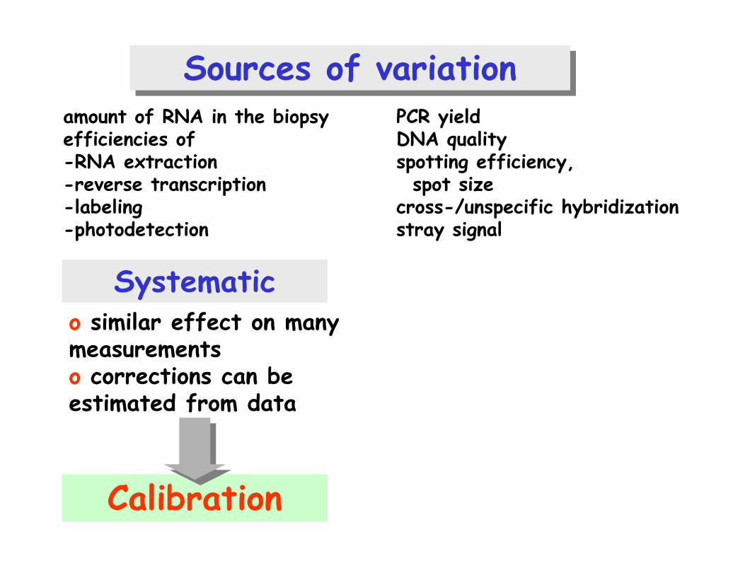
Sources of variationSources of variationamount of RNA in the biopsy efficiencies of-RNA extraction-reverse transcription -labeling-photodetection
PCR yieldDNA qualityspotting efficiency,spot size
cross-/unspecific hybridizationstray signal
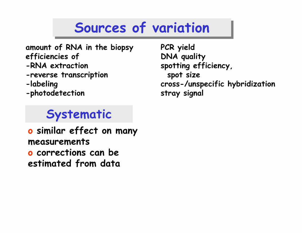
Sources of variationSources of variationamount of RNA in the biopsy efficiencies of-RNA extraction-reverse transcription -labeling-photodetection
PCR yieldDNA qualityspotting efficiency,spot size
cross-/unspecific hybridizationstray signal
Systematico similar effect on many measurementso corrections can be estimated from data
Calibration
Stochastico too random to be ex-plicitely accounted for o “noise”
Error model

Error models
Definition:description of the possible outcomes of a measurement
Depends on:-true value of the measured quantity (abundances of specific molecules in biological sample)
-measurement apparatus (cascade of biochemical reactions, optical detection system with laser scanner or CCD camera)

Error models
Purpose:
1.statistical inference (appropriate parametric methods have better power)
2.summarization (summary statistic instead of full empirical distribution)
3.quality control

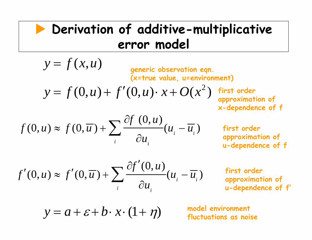
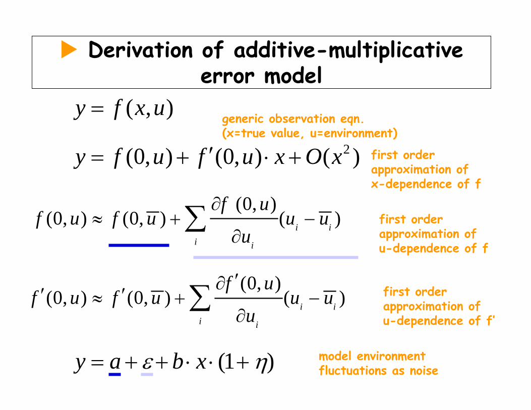
Derivation of additive-multiplicative error model
y = f(x,u)y measurement
f measurement apparatus
x true underlying quantity
u further factors that can influence the measurement (“environment”)

Derivation of additive-multiplicative error model
2
(0, )(0, ) (0, ) ( )
(0, )(0, ) (0, ) ( )
( , )
(0, ) (0, ) ( )
(1 )
i ii i
i ii i
f uf u f u u u
u
f uf u f u u u
u
y f x u
y f u f u x O x
y a b xε η
∂≈ + −
∂
′∂′ ′≈ + −∂
=
′= + ⋅ +
= + + ⋅ ⋅ +
∑
∑

Derivation of additive-multiplicative error model
2
(0, )(0, ) (0, ) ( )
(0, )(0, ) (0, ) ( )
( , )
(0, ) (0, ) ( )
(1 )
i ii i
i ii i
f uf u f u u u
u
f uf u f u u u
u
y f x u
y f u f u x O x
y a b xε η
∂≈ + −
∂
′∂′ ′≈ + −∂
=
′= + ⋅ +
= + + ⋅ ⋅ +
∑
∑
generic observation eqn. (x=true value, u=environment)
first order approximation of x-dependence of f
first order approximation of u-dependence of f
first order approximation of u-dependence of f’
model environment fluctuations as noise
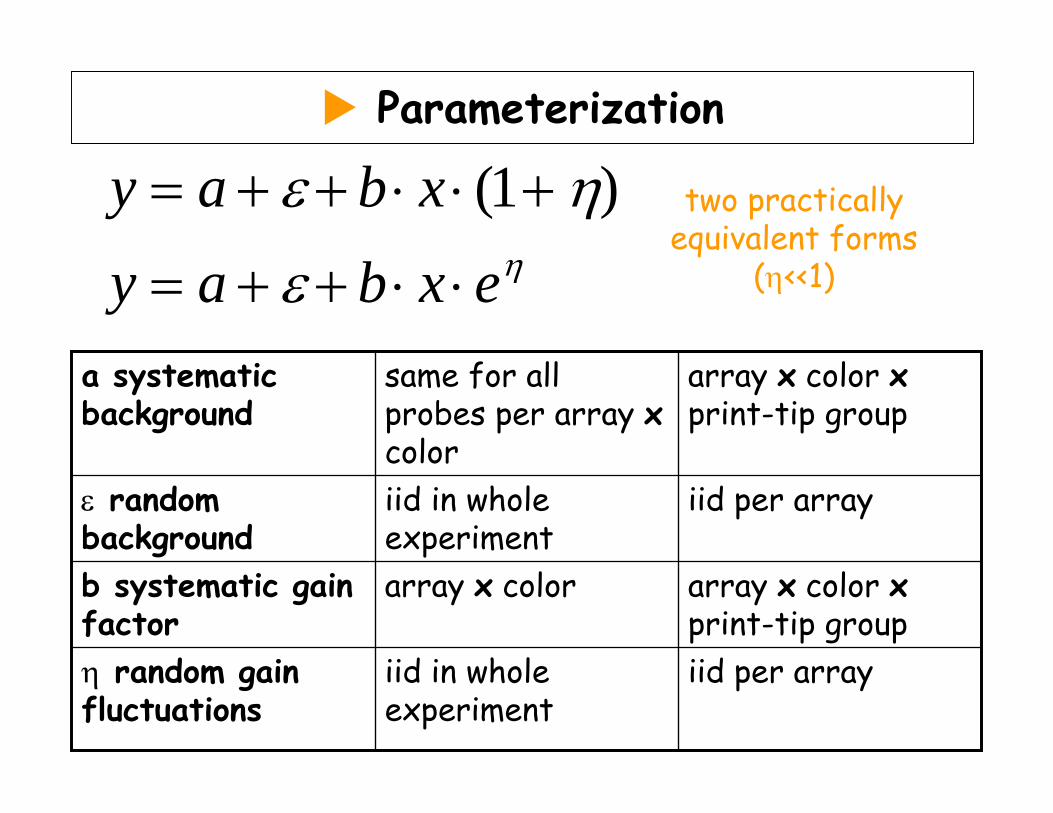
Parameterization
(1 )y a b xy a b x eη
ε η
ε
= + + ⋅ ⋅ +
= + + ⋅ ⋅
two practically equivalent forms
(η<<1)
iid per arrayiid in whole experiment
η random gain fluctuations
array x color xprint-tip group
array x colorb systematic gain factor
iid per arrayiid in whole experiment
ε random background
array x color xprint-tip group
same for all probes per array xcolor
a systematic background
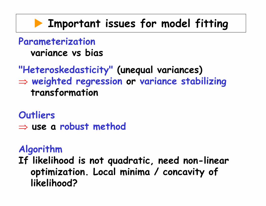
Important issues for model fittingParameterization
variance vs bias
"Heteroskedasticity" (unequal variances)⇒ weighted regression or variance stabilizing
transformation
Outliers⇒ use a robust method
AlgorithmIf likelihood is not quadratic, need non-linear
optimization. Local minima / concavity of likelihood?

The two-component model
raw scale log scaleB. Durbin, D. Rocke, JCB 2001

The two-component model
raw scale log scaleB. Durbin, D. Rocke, JCB 2001
“additive” noise
“multiplicative” noise

Nesting
(1 )' ' ' (1 ')
'' '' '' (1 '')
y a b xx a b z
y a b z
ε ηε η
ε η
= + + ⋅ ⋅ += + + ⋅ ⋅ +
⇓≈ + + ⋅ ⋅ +
e.g. replicate hybridization
e.g. replicate RNA isolation
overall

variance stabilization
Xu a family of random variables with EXu=u, VarXu=v(u).
Define
⇒ var f(Xu ) ≈ independent of u
1( )v( )
x
f x duu
= ∫
derivation: linear approximation

0 20000 40000 60000
8.0
8.5
9.0
9.5
10.0
11.0
raw scale
trans
form
ed s
cale
f(x)
x
variance stabilizing transformation

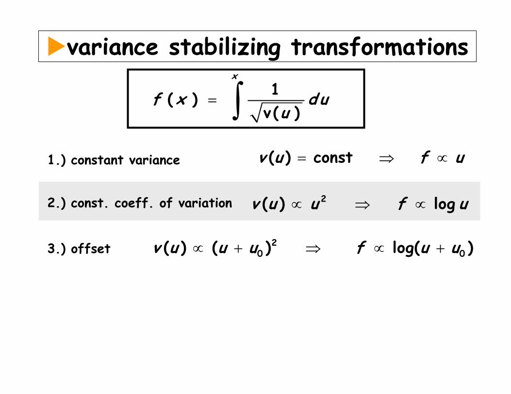
variance stabilizing transformations1( )
v ( )
x
f x d uu
= ∫

variance stabilizing transformations1( )
v ( )
x
f x d uu
= ∫1.) constant variance ( ) constv u f u= ⇒ ∝

variance stabilizing transformations1( )
v ( )
x
f x d uu
= ∫1.) constant variance ( ) constv u f u= ⇒ ∝
2.) const. coeff. of variation 2( ) logv u u f u∝ ⇒ ∝
variance stabilizing transformations1( )
v ( )
x
f x d uu
= ∫1.) constant variance ( ) constv u f u= ⇒ ∝
2.) const. coeff. of variation 2( ) logv u u f u∝ ⇒ ∝
3.) offset 20 0( ) ( ) log( )v u u u f u u∝ + ⇒ ∝ +

variance stabilizing transformations1( )
v ( )
x
f x d uu
= ∫1.) constant variance ( ) constv u f u= ⇒ ∝
2.) const. coeff. of variation 2( ) logv u u f u∝ ⇒ ∝
3.) offset 20 0( ) ( ) log( )v u u u f u u∝ + ⇒ ∝ +
4.) microarray
2 2 00( ) ( ) arsinh u uv u u u s f
s+
∝ + + ⇒ ∝

the arsinh transformation
- - - log u
——— arsinh((u+uo)/c)
( )( )
2arsinh( ) log 1
arsinh log log 2 0limx
x x x
x x→∞
= + +
− − =
intensity-200 0 200 400 600 800 1000
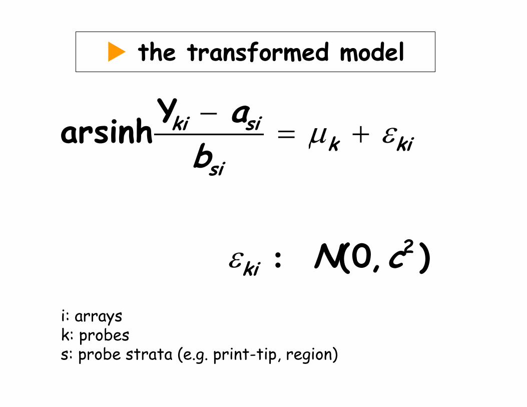
the transformed model
2
Yarsinh
(0, )
sikik ki
si
ki
ab
N c
µ ε
ε
−= +
:
i: arrays k: probess: probe strata (e.g. print-tip, region)

profile log-likelihood
,( , ) sup ( , , , )
cpll a b ll a b c
µµ=

profile log-likelihood
,( , ) sup ( , , , )
cpll a b ll a b c
µµ=
Here:

Least trimmed sum of squares regression
0 2 4 6 8
02
46
8
x
y
2
2
2 2
( )
: min
: min
| med{ }
i i i
ii
ii I
i kk
r y f x
LS r
LTS r
I i r r
∈
= −
→
→
= <
∑
∑
- least sum of squares (LS): Gauss, Legendre ~ 1790- least trimmed sum of squares (LTS): Rousseeuw 1984
x
f(x) = a+bx
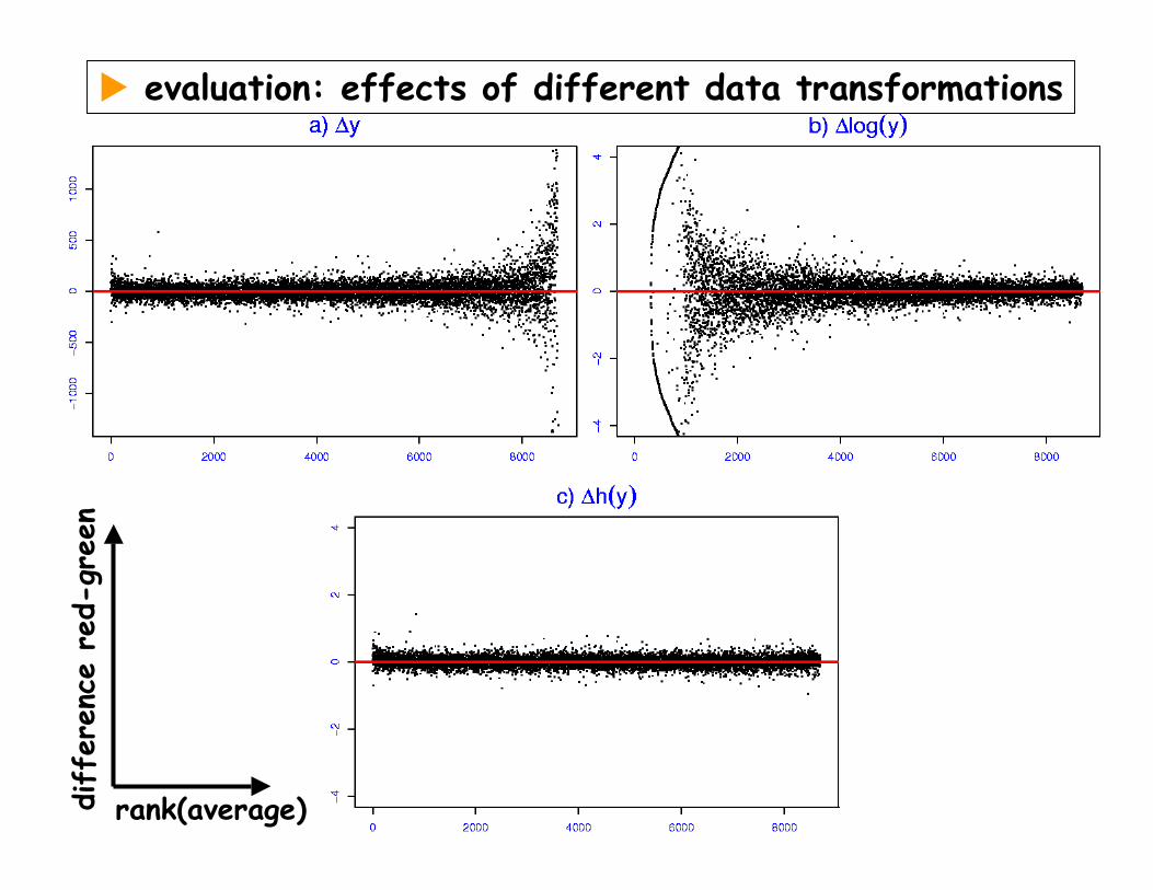
evaluation: effects of different data transformationsdiff
eren
ce r
ed-g
reen
rank(average)
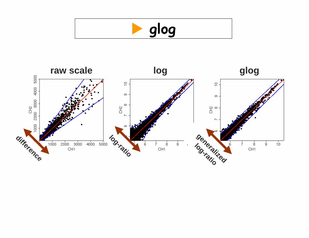
raw scale log glog
difference
log-ratio
generalized
log-ratio
glog

raw scale log glog
difference
log-ratio
generalized
log-ratio
glog
constant partvariance:
proportional part

Motivation for the generalized log-ratio
= −
≈
−−⇒ = −
1 2 2 1
1 2
11 2
( ) ( , ) ( , )( ) Var( ( , )) const.
( , ) inh( ) inh( )s
i h z z h z zii h z z
z az ah z z as asb b
z1, z2 ~ additive-multiplicative error modelSearch function h that fulfills

Properties of the generalized log-ratio
− −= −
= − − −
1 21 2
1 2 1 2
( , ) inh( ) inh( )
( , ) log( ) log( )
z a z ah z z as asb b
q z z z a z a
(i) for z1, z2>>a, h and q are the same
(ii) |h(z1, z2)| ≤ |q(z1, z2)|
(iii) exp(h(z1, z2)) is a shrinkage estimator for fold-change

Properties of the generalized log-ratio
zi=a+ε+bxi exp(η)
x2=0.5…15, x1=2 x2, a=0, σa=1, b=1, σb=0.1

Properties of the generalized log-ratio
zi=a+ε+bxi exp(η)
x2=0.5…15, x1=2 x2, a=0, σa=1, b=1, σb=0.1
Variance-Bias Tradeoff
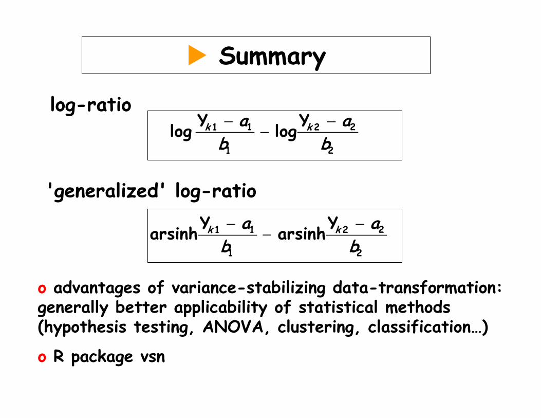
Summary
log-ratio
'generalized' log-ratio
o advantages of variance-stabilizing data-transformation: generally better applicability of statistical methods (hypothesis testing, ANOVA, clustering, classification…)
o R package vsn
1 21 2
1 2
Y Yarsinh arsinhk ka ab b− −
−
1 21 2
1 2
Y Ylog logk ka ab b− −
−

“Single color normalization”
n red-green arrays (R1, G1, R2, G2,… Rn, Gn)
within/between slidesfor (i=1:n)
calculate Mi= log(Ri/Gi), Ai= ½ log(Ri*Gi)normalize Mi vs Ai
normalize M1…Mn
all at oncenormalize the matrix of (R, G)then calculate log-ratios or any other
contrast you like

How to compare and assess different ‘preprocessing’ methods
Normalization = correction for systematic experimental biases + provision of an expression value that can be used subsequently for testing, clustering, classification, modelling.
Quality trade-off: the better the measurements, the less normalization
Variance-Bias trade-off: how do you weigh measurements that have low signal-noise ratio?

How to compare and assess different ‘normalization’ methods?
Normalization :=1. correction for systematic experimental biases2. provision of expression values that can subsequently be used for testing, clustering, classification, modelling…3. provision of a measure of measurement uncertainty
Quality trade-off: the better the measurements, the less need for normalization. Need for “too much” normalization relates to a quality problem.
Variance-Bias trade-off: how do you weigh measurements that have low signal-noise ratio?- just use anyway- ignore- shrink

How to compare and assess different ‘normalization’ methods?
Aesthetic criteriaLogarithm is more beautiful than arsinh
Practical criteraIt takes forever to run vsn. Referees will only accept my paper if it uses the original MAS5.
Silly criteriaThe best method is that that makes all my scatterplots look like straight, slim cigars
Physical criteriaNormalization calculations should be based on physical/chemical model
Economical/political criteriaLife would be so much easier if everybody were just using the same method, who cares which one
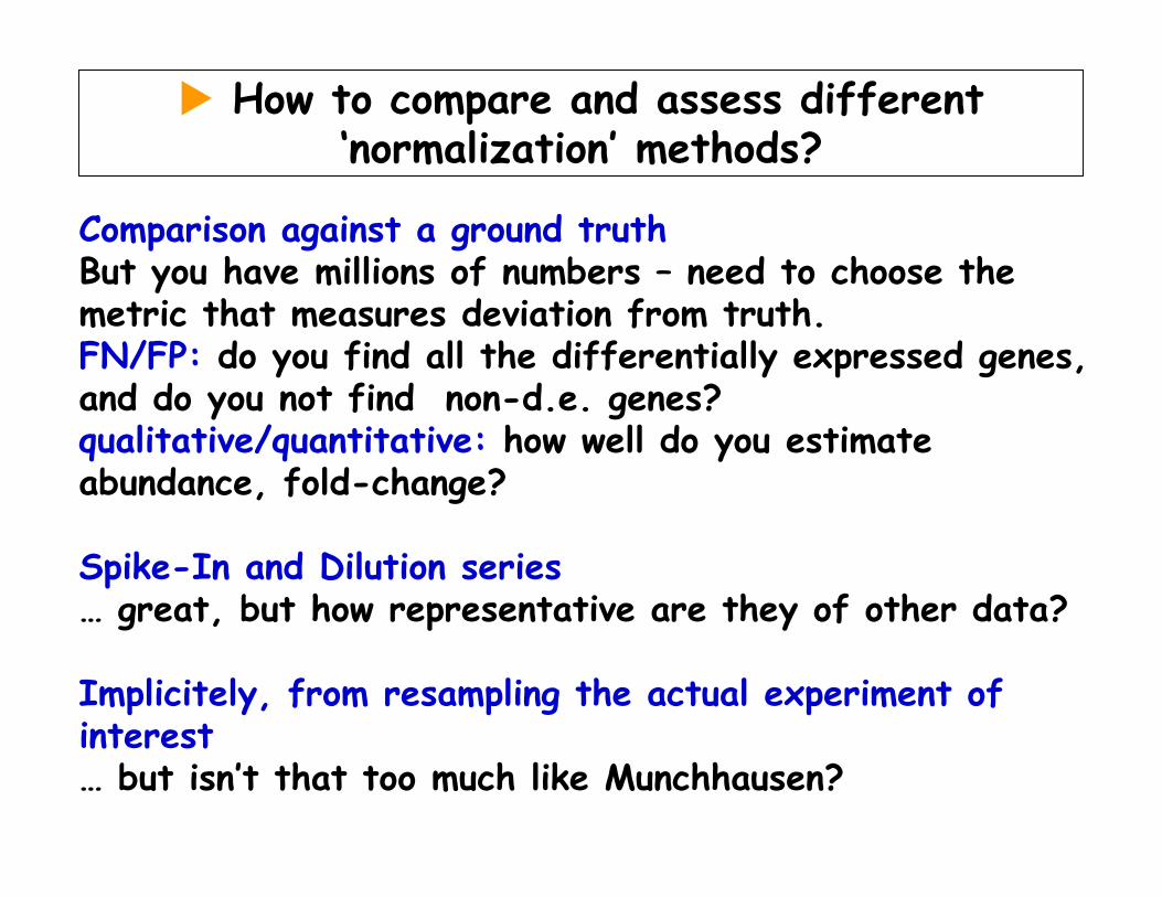
How to compare and assess different ‘normalization’ methods?
Comparison against a ground truthBut you have millions of numbers – need to choose the metric that measures deviation from truth.FN/FP: do you find all the differentially expressed genes, and do you not find non-d.e. genes?qualitative/quantitative: how well do you estimate abundance, fold-change?
Spike-In and Dilution series… great, but how representative are they of other data?
Implicitely, from resampling the actual experiment of interest… but isn’t that too much like Munchhausen?
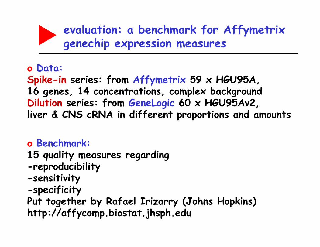
evaluation: a benchmark for Affymetrix genechip expression measures
o Data:Spike-in series: from Affymetrix 59 x HGU95A, 16 genes, 14 concentrations, complex backgroundDilution series: from GeneLogic 60 x HGU95Av2,liver & CNS cRNA in different proportions and amounts
o Benchmark:15 quality measures regarding-reproducibility-sensitivity -specificity Put together by Rafael Irizarry (Johns Hopkins)http://affycomp.biostat.jhsph.edu
evaluation: a benchmark for Affymetrix genechip expression measures
o Package affycomp (on Bioconductor)
o Online competition, accepts contributions via webserver

affycomp results good
bad

ROC curves

Limitations
Affymetrix preprocessing involves(1) PM,MM-synthesis(2) calibration, transformation(3) probe set summarization
‘vsn-scal’ used(1) ignore MM(2) vsn(3) medianpolish (as in RMA, similar to dChip)
This can be improved(1) use MM! (but just not simply PM-MM)(2) stratify by physical probe properties

Resampling method: sensitivity / specificity in detecting differential abundance
o Data: paired tumor/normal tissue from 19 kidney cancers, in color flip duplicates on 38 cDNA slides à 4000 genes.
o 6 different strategies for normalization and quantification of differential abundance
o Calculate for each gene & each method: t-statistics, permutation-p
o For threshold α, compare the number of genes the different methods find, #{pi | pi≤α}
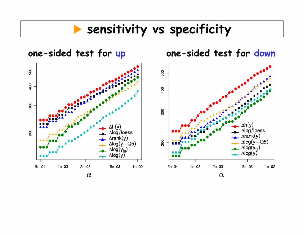
sensitivity vs specificity
one-sided test for up one-sided test for down

Summary
Measuring microarray data is a complex chain of biochemical reactions and physical measurements.
Systematic and stochastic errors
Calibration and error models
Parameter estimation
Getting preprocessing right is prerequisite for getting reasonable results in the end
Improving preprocessing is just like any other technology improvement
How to choose from the plethora of methods?
What’s next
Exercises on data import, diagnostic plots, quality criteria, comparing normalization methods
Lecture on quality control, probe set summaries, hybridization physics

Thank you