wolf of wall street- using - denver spe of wall street.pdf · wolf of wall street- using reservoir...

WOLF OF WALL STREET- USING RESERVOIR ENGINEERING INSIGHT TO

GUIDE OIL AND GAS INVESTMENT DECISIONS

David M. Anderson, Director

Anderson Thompson – Who are we?Anderson Thompson is a team of reservoir engineers,geoscientists, and hydraulic-fracturing specialists, whosemission is to support your efforts to improve the performanceand profitability of your unconventional assets through practicaland innovative field-development optimization

• We partner with oil and gas operators and investors ranging from start-ups to multinationals

• Our team has world-class expertise in unconventional reservoir characterization and production forecasting

• We have broad international basin experience with specialization in the Permian, Eagle Ford, Bakken, Marcellus, and Montney plays

Objectives of this Presentation-

• Learn how to critically evaluate investor and technical presentations and identify the most common fallacies

• See through the “noise” and make better sense of publically available oil and gas data and market research

• Learn how to find hidden opportunities and avoid costly pitfalls when evaluating assets and deciding where to invest

• Understand how reservoir value translates into market value (or how it sometimes doesn’t)

Topics of Discussion – Reservoir Engineering Insights

• Robbing PDP to pay PUD Bakken/Three Forks Example

• If you torture data enough it will confess to anything The peak rate fallacy False causality Mean or median?

• Unrealized potential- the diamond in the rough Identifying upside in assets with existing production Identifying good investment opportunities

Reservoir Engineering Insight #1-

Robbing PDP to pay PUD

Mathistad 2-35H Middle Bakken Well

40-year EUR = 425 Mbblconstant ‘b-value’ of 2.07

Is this a realistic production forecast?

Production Forecast – based on decline curve

Slide Courtesy of Archie Taylor (2010) “Mathistad #1 and #2 Case History - Evaluating Drainage Fracturing, Well Performance and Optimum Spacing in the Bakken and Three Forks” presented at the SPE ATW “Maximizing Tight Oil in the Bakken”

Mathistad 2-35H Bakken Well Location

McKenzie County

Cross Section View of Mathistad Wells


Plan View of Mathistad Wells

Bakken and Three Forks wells have unbounded lateral drainage


Mathistad 2-35MB Updated Production

Decline Curve Analysisb-value = 2.0740-year EUR = 425 Mbbl

Forecast- Decline Curve Analysis (DCA)

bi

i

tbDqq /1)1( +

=

b value Reservoir Drive Mechanism

0 (exponential) Single phase liquid expansion (oil above bubble point), single phase gas expansion at high pressure, water or gas breakthrough in an oil well

0.1 – 0.4 Solution gas drive

0.4 – 0.5 Single phase gas expansion

0.5 Effective edge water drive

0.5 – 1 Layered reservoirs

1 – 1.5 Transitional flow in multi-stage hz wells frac’d reservoirs

2 Linear flow

The Hyperbolic Decline Curve

Initial decline rate

Initial production rate

Decline Curves 101

Hyperbolic exponent

1320 ft well spacing case40-year EUR = 412 Mbbl


Forecast Comparison- DCA vs. Model Based

Model supports DCA assuming 320 acre drainage

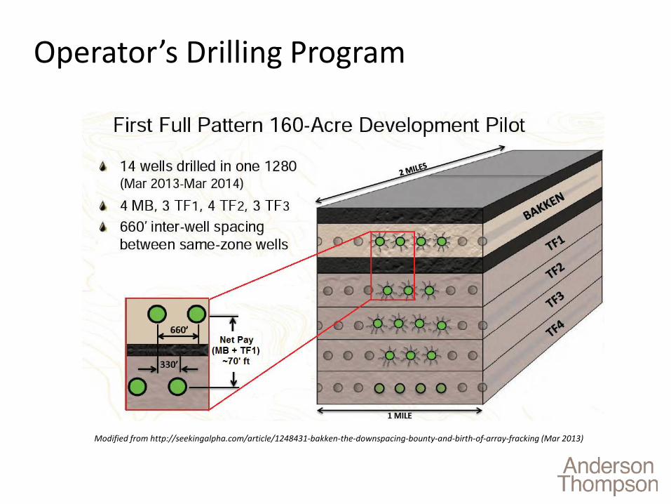
Operator’s Drilling Program

Modified from http://seekingalpha.com/article/1248431-bakken-the-downspacing-bounty-and-birth-of-array-fracking (Mar 2013)

Reservoir Models- Base Case vs. Infill

1320 ft

320 acre drainage area per well

660 ft

160 acre drainage area per well

Production Forecasts- Base Case vs. Infill

660 ft well spacing160 acre case

1320 ft well spacing320 acre case


Robbing PDP to pay PUD- Summary• Production decline changes when infill wells are drilled!• DCA-based type curves are usually not adjusted to account

for the impact of infill drilling programs• The optimum drilling density in a field development scenario

often requires “robbing PDP to pay PUD!”

400

600

800

1000

1200

1400

1600

20

30

40

50

60

70

80

90

100

110

1 2 3 4 5 6 7 8

NPV EUR

NPV($MM)

EUR/Well(Mbbl)

Wells / DSU

EUR/well begins to drop due to infill drilling

Optimum drilling density for NPV

Reservoir Engineering Insight #2-If you torture data enough, it will

confess to anything

0

50000

100000

150000

200000

250000

0 1000 2000 3000 4000 5000 6000 7000 8000 9000 10000

5 Ye

ar N

p (S

TB)

1 calendar month Np (STB)

1 Calendar Month Np vs 5 Year Np

WELLS ON PRODUCTION FROM 2007 WELLS ON PRODUCTION FROM 2002 WELLS ON PRODUCTION FROM 1997

WELLS ON PRODUCTION FROM 1992 WELLS ON PRODUCTION FROM 1987

The Fallacy of the 30 day IP (or peak rate)

All producing oil wells in Alberta since 1987-

- Wells with high initial productivity often do not perform well in the long-term (and vice-versa)

Why??

Initial production rates are DOMINATED by operations during the first few weeks- long term reservoir capability is usually MASKED

The Fallacy of the 30 day IP (or peak rate)

0

50000

100000

150000

200000

250000

0 2000 4000 6000 8000 10000 12000 14000 16000 18000 20000

5 Ye

ar N

p (S

TB)

3 calendar month Np (STB)

3 Calendar Month Np vs 5 Year Np

WELLS ON PRODUCTION FROM 2007 WELLS ON PRODUCTION FROM 2002WELLS ON PRODUCTION FROM 1997 WELLS ON PRODUCTION FROM 1992WELLS ON PRODUCTION FROM 1987

Correlation is better for 90 day (3 month) rate but still poor R2<0.5

Calendar Time IP or Producing Time IP?

Calendar Time IP is biased towards wells with low downtime and/or high drawdown

Producing Time IP is biased towards wells with high downtime and/or low drawdown

Courtesy of Bertrand Groulx

Correlating Early Production Indicators to EUR

Courtesy of Bertrand Groulx

Example of Peak Rate Fallacy

Well 1Well 2Which is the better well?

Use Rate Transient Analysis to Reveal the Truth!

Well 1Well 2Which is the better well?

Well 1Well 2

Function of rates AND flowing pressuresFlatter = betterWell 2 is the better well!

RTA (reservoir model) Forecasts

Well 1Well 2

Well 1Well 2

Production update- confirms early predictions

False Causality

• Belief that correlation proves causation

• Examples- Sleeping with one’s shoes on is strongly correlated with

waking up with a headache. Therefore sleeping with shoes on causes headaches

As ice cream sales increase, the rate of drowning deaths increases sharply. Therefore, ice cream consumption causes drowning

False Causality in Oil and Gas Data• Proppant “X” is correlated with better well performance in

the Eagle Ford. Therefore using proppant X will result in better well performance

0100200300400500600700800900

100 mesh 20/40 30/50 Proppant X

Correlation Between Average Peak Rate and Proppant Type

• Reservoir engineering insight- Proppant “X” was used by a single operator with the best land position in the EF; Operator also known for flowing back wells unchoked (to maximize 30-90 day production)

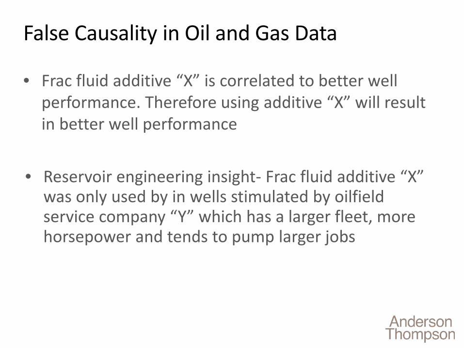
False Causality in Oil and Gas Data

• Frac fluid additive “X” is correlated to better well performance. Therefore using additive “X” will result in better well performance

• Reservoir engineering insight- Frac fluid additive “X” was only used by in wells stimulated by oilfield service company “Y” which has a larger fleet, more horsepower and tends to pump larger jobs

What Really Drives Well Performance?Pr

oduc

tion

rate

Time

Operations- Open vs choked flow- Shut-ins- Flowing pressure profile- Artificial lift- Separator pressure/temp

Reservoir/Fluid- Reservoir pressure- Net pay- Porosity- Sw- Young’s modulus- Poisson’s ratio- Natural fractures- Stress profile- Permeability- Fluid compressibility- Pore compressibility- Fluid viscosity- Gas solubility- Gas gravity- Oil API gravity- Capillary pressure

Completion/Wellbore- Lateral length- Landing depth- Tubing/casing size/depth- Number of entry points- Missed entry points- Completion type- Proppant volume- Proppant type- Fluid volume- Fluid type- Treatment schedule- Well spacing

Just one of many variables that influence well performance

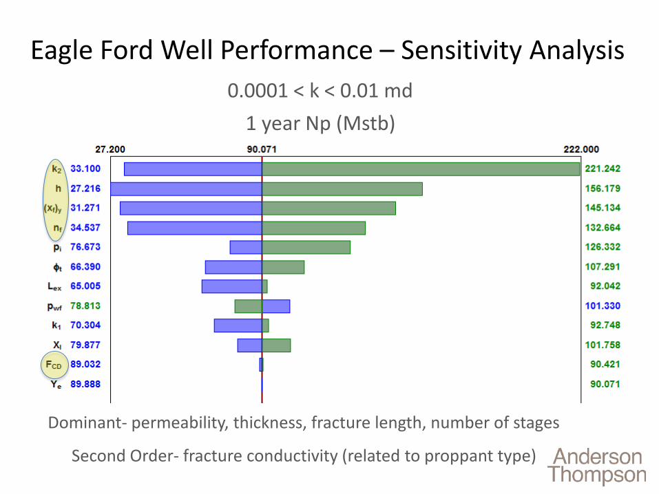
Dominant- permeability, thickness, fracture length, number of stages

Second Order- fracture conductivity (related to proppant type)

1 year Np (Mstb)

Eagle Ford Well Performance – Sensitivity Analysis0.0001 < k < 0.01 md

False Causality

• Beware of “sweeping conclusions of causality” that are based on two dimensional correlations

• The vast majority of well performance variance results from differences in the rock and reservoir fluids

• Reservoir engineering insight will find the true underlying performance drivers that are specific to the play of interest

Statistics 101- Mean or Median?

Median (P50) EUR = 150 Mstb Mean EUR = 205 Mstb

Cumulative Distribution of EURs in Bone Spring, Lea County

102

103

104

3 . 104

4 . 101

6

2

3

4

6

2

3

4

6

2

Op

Gas

Rat

e (M

scfd

)

95

0

5

10

15

20

25

30

35

40

45

50

55

60

65

70

75

80

85

90

No. of P

roducing Wells

0 5 10 15 20 25 30 35 40 45 50 55 60 65 70 75 80 85 90 95 100 105 110 115 120

Normalized Time (month)

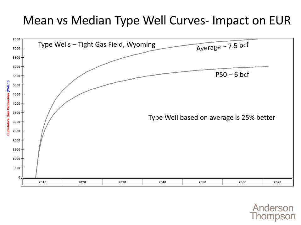
Mean vs Median Type Well Curves

Type Wells – Tight Gas Field, Wyoming

Mean (Average)

P50

7500

0

500

1000

1500

2000

2500

3000

3500

4000

4500

5000

5500

6000

6500

7000

Cum

ulat

ive

Gas

Pro

duct

ion

(MM

scf)

2010 2020 2030 2040 2050 2060 2070

Mean vs Median Type Well Curves- Impact on EUR

Type Wells – Tight Gas Field, Wyoming

P50 – 6 bcf

Type Well based on average is 25% better

Mean or Median?

• Median is a better indicator of how a new well is likely to perform

• Mean is the average- in a log normal distribution, mean is higher than the median

• E&Ps that use type curves based on mean are likely overstating the value of undrilled acreage, especially for small drilling programs

• Type well curves created using limited statistical samples are unreliable

Reservoir Engineering Insight #3-Unrealized potential- the diamond in the rough

Using Reservoir Insights to Find Opportunity

• How can reservoir engineering insight be used to identify underperforming assets?

• How closely can value created in the reservoir be correlated to shareholder and market value?

Example 1- Insufficient Pipeline Capacity

- Drop in production rate- Increase in decline rate- No loss in productivity!- Model – OGIP = 24 bcf- Recoverable Gas – 18 bcf

Increasing back pressure due to reduced pipeline capacity

Simulated and m

easured bhp(psia)

Gas

Rat

e (M

Msc

fd)

Example 1- Do Nothing or Remove Back Pressure

EUR = 3 bcfBased on current conditions

EUR = 18 bcf if back pressure is removed!

Example 2- Productivity Loss

103

104

2 . 104

4 . 102

56

8

2

3

4

56

8

Op

Gas

Rat

e (M

scfd

)

3.800.00 0.20 0.40 0.60 0.80 1.00 1.20 1.40 1.60 1.80 2.00 2.20 2.40 2.60 2.80 3.00 3.20 3.40 3.60

Normalized Time (month)

Gas Well 1

Gas Well 2

Which well is underperforming?

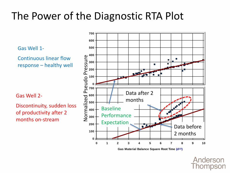
The Power of the Diagnostic RTA Plot

Superposition TimeNMC #M-1H

700

0

100

200

300

400

500

600

100 1 2 3 4 5 6 7 8 9

Gas Material Balance Square Root Time (d1/2)

0

100

200

300

400

500

600

700

Gas Well 1-

Continuous linear flow response – healthy well

Gas Well 2-

Discontinuity, sudden loss of productivity after 2 months on-stream N

orm

alize

d Ps

eudo

Pre

ssur

eData after 2 months

Data before 2 months

Baseline Performance Expectation

Identifying Common Well Performance Issues

Surface Wellbore Completion / Reservoir- Low pump efficiency- Insufficient compression- Insufficient pipeline

capacity- Chokes / restrictions

- Mechanical blockage (Unmilled ball seats, parted casing, proppant bridge etc)

- Liquid loading- Buildup of precipitates- Underperforming artificial lift

- Frac face skin- Low frac conductivity- Fines migration- Stress dependent flow capacity- Phase trapping- Interference- Water influx

- Drop in rate- Increase in decline

rate

- Inconsistent flowing pressure response

- High measured bhp- Noisy production data

- Divergence between model and data

- Low measured bhp

Issues

Symptoms

Resolution EasyLow risk

How to diagnose it

- Look at production data

- Use RTA / modeling- Pipeline modeling

Moderate DifficultyMedium risk

DifficultHigh risk

- Use RTA / modeling- Downhole camera- Measure bhp

- Use RTA / modeling- Tracers / PLT- PBU test

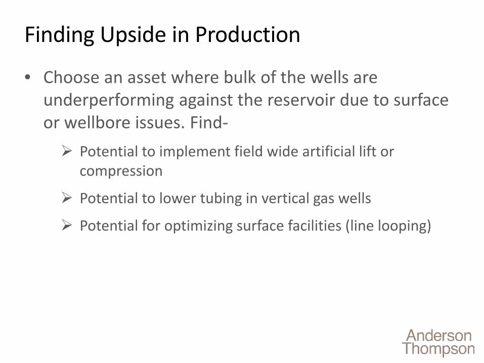
Finding Upside in Production

• Choose an asset where bulk of the wells are underperforming against the reservoir due to surface or wellbore issues. Find- Potential to implement field wide artificial lift or

compression

Potential to lower tubing in vertical gas wells

Potential for optimizing surface facilities (line looping)

Translating Reservoir Value into Market Value

• Who are the most successful oil companies?

• Why are they successful?

• How are value and success measured? IP- 30 day or 365 day?

Time to payout and cash flow

NPV and IRR

Repeatability and scalability with low risk

Optimized reservoir management isn’t always rewarded in the market, but it will almost always

provide the best NPV for the asset

Strategies that Oil Companies UseShort Term

- Maximize IP- Minimize D&C cost- Find the sweet spot- Pursue aggressive completion and

treatment designs- Value measured using time to payout- Value measured well by well

Long Term

- Maximize ultimate recovery of the entire asset- Focus on integration of disciplines- Focus on understanding the reservoir- Focus on controlled optimization- Value measured using NPV and IRR- Value measured at the asset level

- Short term strategies are required to put startups and juniors on the map

- Short term strategies are not easily repeatable or scalable

- Companies with successful short term strategies are often overvalued by the stock market

- Long term strategies are boring and often go unnoticed

- Operators employing long term strategies are usually successful across multiple plays/basins

- Small companies with successful long term strategies are often undervalued by the stock market

- Every one of the worlds top 25 oil companies employs long term strategies

Example of Opposing Oilfield Strategies- Montney

• Operator A Minimizes D&C cost by avoiding directional drilling and using

uncemented liners

Drills toe up through multiple benches to maximize total reservoir exposure; contributes to high IP and better liquids recovery

Large proppant volumes per stage maximizes frac area and connection to reservoir; contributes to high IP

Flows back wells unchoked to maximize IP and minimize payout time

Example of Opposing Oilfield Strategies- Montney

• Operator B Spends more on D&C; drills directionally to stay in zone, uses

cemented liner with pinpoint completion technology

Uses high stage density with lower proppant volumes per stage to maximize recovery efficiency in zone and along the lateral

Flows back wells on choke to manage liquids recovery and maintain reservoir pressure above dew point for as long as possible

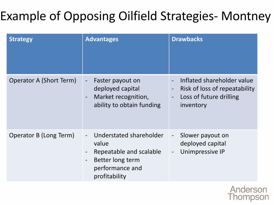
Example of Opposing Oilfield Strategies- MontneyStrategy Advantages Drawbacks

Operator A (Short Term) - Faster payout on deployed capital

- Market recognition, ability to obtain funding

- Inflated shareholder value- Risk of loss of repeatability- Loss of future drilling

inventory

Operator B (Long Term) - Understated shareholder value

- Repeatable and scalable- Better long term

performance and profitability

- Slower payout on deployed capital

- Unimpressive IP

Final Thoughts• Reservoir engineering insight can be useful in the investment

community Helps identify red flags

Helps filter out noise; focus on what is important

Identifies underperforming assets

Helps identify undervalued (or overvalued) companies

• Successful operators and management teams: Are very clear on how they measure value

Can execute a repeatable and scalable development strategy

Don’t have a “silver bullet” but rather, perform to a consistent level of competence across all disciplines in the value chain

Thank-you!

Questions?

wolf of wall street- using - denver spe of wall street.pdf · wolf of wall street- using reservoir...

Documents