(without author's pcnnission) · (without author's pcnnission) 1+1 national library of...
TRANSCRIPT
CENTRE FOR NEWFOUNDI .AND STUDIES
TOTAL OF 10 PAGES ONLY MAY BE XEROXED
(Without Author's Pcnnission)


1+1 National Library of Canada
Bibliotheque nationale du Canada
Acquisitions and Bibliographic Services
Acquisisitons et services bibliographiques
395 Wellington Street Ottawa ON K1A ON4 Canada
395, rue Wellington Ottawa ON K1A ON4 Canada
The author has granted a nonexclusive licence allowing the National Library of Canada to reproduce, loan, distribute or sell copies of this thesis in microform, paper or electronic formats.
The author retains ownership of the copyright in this thesis. Neither the thesis nor substantial extracts from it may be printed or otherwise reproduced without the author's permission.
In compliance with the Canadian Privacy Act some supporting forms may have been removed from this dissertation.
While these forms may be included in the document page count, their removal does not represent any loss of content from the dissertation.
Canada
Your file Votre reference ISBN: 0-612-93014-9 Our file Notre reference ISBN: 0-612-93014-9
L'auteur a accorde une licence non exclusive permettant a Ia Bibliotheque nationale du Canada de reproduire, preter, distribuer ou vendre des copies de cette these sous Ia forme de microfiche/film, de reproduction sur papier ou sur format electronique.
L'auteur conserve Ia propriete du droit d'auteur qui protege cette these. Ni Ia these ni des extraits substantiels de celle-ci ne doivent etre imprimes ou aturement reproduits sans son autorisation.
Conformement a Ia loi canadienne sur Ia protection de Ia vie privee, quelques formulaires secondaires ont ete enleves de ce manuscrit.
Bien que ces formulaires aient inclus dans Ia pagination, il n'y aura aucun contenu manquant.


Simplified Fuzzy Logic Controller Based Vector Control of an Interior Permanent Magnet Motor
St. John's
by
Casey Benjamin Butt
A thesis submitted to the school of graduate studies in partial fulfillment of the requirements for the degree of
Master of Engineering
Faculty of Engineering and Applied Science Memorial University ofNewfoundland
July 2003
Newfoundland Canada
Abstract
In recent years, the interior permanent magnet synchronous motor (IPMSM)
has become increasingly popular for use in high performance drive (HPD) applica
tions due to desirable features such as high torque to current ratio, high power to
weight ratio, high efficiency, low noise and robust operation. As a consequence,
the control of the IPMSM for use in high precision industrial drives has received
heightened attention. This proposed research is directed to develop and implement
a complete and practical vector control scheme for the IPMSM to be used in such
applications.
This thesis presents the control of the IPMSM at rated speed and below, in
the constant torque mode, by use of the maximum torque per ampere (MTPA)
mode of operation utilizing an innovative Taylor series approximated approach.
Coupled with this method is the development of a simplified fuzzy logic controller
(FLC) based speed controller that maintains high performance standards while re
ducing complexity and computational burden. The performance of this proposed
technique is evaluated by simulation as well as by experimental results. A com
parison is made, in simulation, between a more conventional FLC based control
technique with ict = 0 and the proposed simplified FLC with MTP A approach.
The complete vector control scheme is implemented in real-time using a
digital signal processor (DSP) controller board in a laboratory 1 hp interior perma
nent magnet synchronous motor.
ii

Acknowledgements
. I would like to express my sincere gratitude and appreciation to my supervi
sor Professor M. A. Rahman for his guidance, encouragement, advice and tutelage
throughout the preparation of this thesis. His influence has helped me learn the
practicalities of modem research and scientific writing.
I would like to sincerely thank the School of Graduate Studies, the Faculty
of Engineering and Applied Science and Dr. Rahman for their financial support,
without which the pursuit of this research would not have been possible. In addi
tion, I would like to acknowledge Mr. Richard Newman for his expertise and assis
tance with the implementation of the lab equipment.
Finally, I would like to thank my wife Kimberley, my parents Mr. Benjamin
Butt and Mrs. Mary Butt, and my wife's family for their support and encourage
ment, without which it would not have been possible for me to complete this study.
iii
Contents
Abstract ii
Acknowledgements iii
~~~~ ~
List of Symbols xii
lfuk~~oo 1
1.1 General Introduction to Motor Drives....... ..... ... ........... . . ......... . 1
1.1.1 General Review of Electric Motor Drives.... . .... .. .. .. .. .. . ... . 2
1.2 Permanent Magnet Synchronous Motors...... .. . . . . . . . . . . . . . . . . . . . . . . ... 4
1.2.1 General Introduction................................ .... ... ......... 4
1.2.2 Classification of PM synchronous motors. . .... . ....... ... ... ... 5
1.3 PMSMDrives... ... ... .. ... . ... ...... . .. . ...... .. .... .. ....... .... . . ... ...... 8
1.3.1 Vector Control Schemes............... . ............ .. . ... .. . ... ... 8
1.3.2 PMSM Drive Controllers.. .. . ... .. ................. .... .. . ..... . .... 12
1.3.3 PMSM Drives with Adaptive Controllers.... . ..... .. .. . .. ........ 18
1.3.4 PMSM Drives with Intelligent Controllers.... ...... ..... .... .... 21
1.4 Problem Identification and Thesis Objectives. ..... ... ... .. .. .. ....... .. 25
1.5 Thesis Organization... .. ... .... ... ... .... ...... .... .. .. .... . ... .. ..... .. .. .. 27
IV
2 Analysis and Modeling of the PWM VSI-Fed IPMSM Drive 28
2.1 General Introduction.... . . . . . . . . . . . . . . . . . . . . . . . . . . . . . . . . . . . . . . . . . . . . . . . . . . .. 28
2.1.1 Mathematical Modeling of the IPMSM........... .. . ... .. . .. ..... 29
2.2 Vector Control of the IPMSM Drive..... ....... .. ... .... ... ...... ... .... 37
2.2.1 Maximum Torque Per Ampere Speed controller..... . .......... 40
2.2.2 Vector rotator...................... ... .... ... .... . ........ . .. ... ..... 44
2.2.3 Current Controller and Voltage Source Inverter... .. ... . ...... 44
2.3 Current Control of the Voltage Source Inverter. .. .. .... .. ... . .. . ...... 45
2.3.1 Effect of Unconnected Neutrals ......... . ... ..... ........ . ..... .. 48
2.3.2 Limitation of de Bus Voltage and Inverter Switching
Frequency.............. .. ... . . . . . . . . . . . . . . . . . . . . . .. . . . . . . . . . . . . . . . . . . 48
2.4 Hysteresis Current Controller..................... .... .. ... ... ...... .. ..... 50
3 Fuzzy Logic Based Speed Controller 53
3.1 General Introduction. ........ ... ........ . .. .. .... .. .. ...... ................ 53
3.2 Fundamentals of Fuzzy Logic Control.... ... .. ........... ..... . ... .... 54
3.2.1 Fuzzification..................... ... . . . . . . . . . . . . . . . . . . . . . . . . . . . . . . . . . . . 57
3.2.2 Rule Evaluation.. ..... .. .. .. .. ....... .. ...... . .. ...... . .... . .. ..... ... 57
3.2.3 Aggregation and Defuzzification...... ........ . .. . .. .. . . . . . . ... . .... 58
3.3 Fuzzy Logic Controller for IPMSM Drive... . ... .. .. ....... ..... ...... 60
3.3.1 FLC Structure for the IPMSM Drive........................... ... 61
3.3.2 Simplified FLC for the IPMSM Drive.... . .. ........... .. . .. . .... .. 64
3.4 Concluding Remarks.... .. ..... .. ... ... .... .. ............ . .... ........ .... 67
4 Simulation of the FLC Based Vector Control of the IPMSM 68
4.1 General Introduction... .. .... ..... . ... ... .. .... .... .. ........... .. .. .... ... 68
v

4.2 Current Controller and Voltage Source Inverter......... . ..... ..... 69
4.3 Simulation Results and Discussion..................... . ... .......... 69
4.4 Concluding Remarks....................................... . ............ 95
5 Experimental Implementation of the Simplified FLC Based MTP A Vec
tor Control of the IPMSM 96
5.1 General Introduction.. ......... . ... .... .... ... ... ... .......... ...... .. ... 96
5.2 Experimental Setup.. .... ... . ... . ... ... ................ .... .. ..... .... ... 97
5.2.1 Hardware Implementation...................................... .. ..... 97
5.2.2 Software Implementation.............................. ... ... . ......... 99
5.3 Experimental Results and Discussion......................... ... .. ... 106
5.4 Concluding Remarks. . . . . . . . . . . . . . . . . . . . . . . . . . . . . . . . . . . . . . . . . . . . . . . . . . . . 115
6 Conclusions 116
6.1 General........................................ ...... ......... ...... .. ... 116
6.2 Major Contributions of this Work.... ... . ........ . ...... .. . ..... . . .. 118
6.3 Future Direction of Research...................... . ................. 119
6.4 Conclusions..... .... . .. ........... .... .. .... ..... ........ .... ... ... .... . 119
References
Appendix A
Appendix B
Appendix C
AppendixD
Vl
121
133
134
146
151
List of Figures
1.1 Direct vector control scheme ofPMSM....... .................................. 10
1.2 Indirect vector control scheme ofPMSM. . .. . . . . .. . . . .. . . . . . .. . . .. . .. . .. . ...... 11
2.1 Relative positions of stationary d-q axes and rotating dr-qr axes...... .... ... 33
2.2 Equivalent circuit model of the IPMSM: (a) d-axis, (b) q-axis.. .. ....... .... 36
2.3 Vector diagram ofiPMSM parameters............................. .. ........... 39
2.4 Block diagram of complete current-controlled VSI-fed IPMSM drive...... 39
2.5 Maximum torque per ampere (MTPA) trajectory on constant torque loci . .. 41
2.6 Current controlled voltage source inverter for the IPMSM drive............. 45
2.7 VSI voltage vectors....................... .. ................................. . ...... 47
2.8 Hysteresis current controller switching pattern..... . ..................... ....... 50
2.9 Fixed-band hysteresis current controller scheme. ....... . . . . . . . . . . . . . . . . . . . . . . . . 52
2.10 Fixed-band hysteresis current controller waveforms......... .. .. ... . ... ... .... 52
3.1 Membership functions of linguistic value ZE: (a) triangular, (b) Gaussian func
tion, (c) trapezoidal and (d) singleton............................... .. ............ 55
3.2 Overview of the complete fuzzy inference............ .......... . ... .. . .......... 59
3.3 Block diagram of proposed simplified FLC-based IPMSM drive with MTPA
c.ontrol. ........... ... . . . . . . . . . . . . . . . . .. ..... ......... .. .. ............ ..... .. . .... .. . .. 65
3.4 Membership functions for: (a) normalized speed error ~corn , (b) normalized
command torque Ten*.. ...................... . ............ . .. .. .... . ...... .. . . . . . . . . 66
Vll
4.1 Simulated responses of the FLC based/id=O IPMSM drive: a) speed, (b) com
mand phase current, (c) q-axis command current and (d) steady-state actual
phase current at no load and rated speed conditions.. .. .. ...................... 76
4.2 Simulated responses of the FLC based/id=O IPMSM drive: a) speed, (b) com
mand phase current, (c) q-axis command current and (d) steady-state actual
phase current at half load and rated speed conditions..... . ... . . . . . . . . ... . . . . . . . 77
4.3 Simulated responses of the FLC based/id=O IPMSM drive: a) speed, (b) com-
mand phase current, (c) q-axis command current and (d) steady-state actual
phase current at full load and rated speed conditions..... . .... ............ . . . . . 78
4.4 Simulated responses of the FLC based/id=O IPMSM drive: a) speed, (b) com
mand phase current, (c) q-axis command current and (d) steady-state actual
phase current for a step change of speed at halfload conditions.. . ... .. .. ... 79
4.5 Simulated responses of the FLC based/id=O IPMSM drive: a) speed, (b) com
mand phase current, (c) q-axis command current and (d) steady-state actual
phase current for a sudden change of load (from half load to full load) at rated
speed..... . ...... ........... . .. . ..... . . .................. . ...... ...... . ..... . .......... 80
4.6 Simulated responses of the simplified FLC based/MTPA IPMSM drive: a)
speed, (b) command phase current, (c) q-axis and d-axis command currents
and (d) steady-state actual phase current at no load and rated speed condi-
tions.... . ........ . ........... . ............ ..... .. . ........ . . . ... . .. ... . .. .. .. .. . ...... 81
4.7 Simulated responses of the simplified FLC based/MTPA IPMSM drive: a)
speed, (b) steady-state actual phase current, (c) q-axis and d-axis command
currents and (d) steady-state actual phase currents ia and ib at half load and
rated speed conditions.. . .. . ..... ...................... . ..... . ... ....... . .... . ... .. 82
4.8 Simulated responses of the simplified FLC based/MTP A IPMSM drive: a)
speed, (b) steady-state actual phase current, (c) q-axis and d-axis command
viii
currents and (d) steady-state actual phase currents ia, ib and ic at full load and
rated speed conditions.................... . . . . . . . . . . . . . . . . . . . . . . . . . . . . . . . . . . . . . . . . . 83
4.9 Simulated responses of the simplified FLC based!MTPA IPMSM drive: a)
speed, (b) steady-state actual phase current, (c) q-axis and d-axis command
currents and (d) steady-state actual phase currents ia, ib and ic at full load +
25% and rated speed conditions...................... .. .. . ...... .. ........ . ...... 84
4.10 Simulated responses of the simplified FLC based/MTPA IPMSM drive: a)
speed, (b) steady-state actual phase current, (c) q-axis and d-axis command
currents and (d) steady-state actual phase currents ia, ib and ic at full load and
low speed (75 rad./sec.) conditions... .. . .. ..... .................................. 85
4.11 Simulated responses of the simplified FLC based!MTPA IPMSM drive: a)
speed, (b) steady-state actual phase current, (c) q-axis and d-axis command
currents and (d) steady-state actual phase currents ia, ib and ic for a step
change of speed at halfload conditions.................. . ...... . . .... . ..... . .... 86
4.12 Simulated responses of the simplified FLC based!MTP A IPMSM drive: a)
speed, (b) steady-state actual phase current, (c) q-axis and d-axis command
currents and (d) steady-state actual and command phase currents ia and ia * for
a step change of speed at full load conditions...................... . .. . ...... ... 87
4.13 Simulated responses of the simplified FLC based!MTPA IPMSM drive: a)
speed, (b) command phase current, (c) q-axis and d-axis command currents
and (d) steady-state actual phase current ia for a sudden change ofload (from
halfload to full load) at rated speed... .. ................ . .. . .. ..... .. .. .... . .. . ... 88
4.14 Simulated responses of the simplified FLC based!MTPA IPMSM drive: a)
speed, (b) steady-state actual phase current ia for a sudden change of stator re
sistance (R to 2R) at no load and rated speed.... ......... .. ... .... .. .. . . . . . . . . . 89
ix

4.15 Simulated responses of the simplified FLC based/MTPA IPMSM drive: a)
speed, (b) steady-state actual phase current ia for a sudden change of stator re
sistance (R to 2R) at full load and rated speed........ . . . . . . . . .. . . . . . . . . . . . . . ... . 90
4.16 Simulated responses of the simplified FLC based/MTPA IPMSM drive: a)
speed, (b) steady-state actual phase current ia for a sudden change of rotor in
ertia (J to 21) at no load and rated speed......... .................... ... .. .. . ..... 91
4.17 Simulated responses of the simplified FLC based/MTP A IPMSM drive: a)
speed, (b) steady-state actual phase current ia for a sudden change of rotor in
ertia (J to 21) at full load and rated speed.. . . . . . . . . . . . . . . . . . . . . . . . . . . . . . . . . . . . . . . . 92
4.18 Simulated responses of the simplified FLC based/MTPA IPMSM drive: a)
speed, (b) steady-state actual phase current ia for a sudden 50% decrease of Lq
at no load and rated speed.. . . . . . . . . . . . . . . . . . . . . . . . . . . . . . . . . . . . . . . . . . . . . . . . . . . . . . . . . . 93
4.19 Simulated responses of the simplified FLC based/MTPA IPMSM drive: a)
speed, (b) steady-state actual phase current ia for a sudden 50% decrease ofLq
at full load and rated speed........... . .............. .. ................... ... .. . ..... 94
5.1 Hardware schematic for experimental implementation ofthe IPMSM drive. 99
5.2 Flow chart of the software for real-time implementation of the FLC based
IPMSM drive. ..... . .. . .... ...... ................................ . ........... . ...... 105
5.3 Experimental responses of the simplified FLC based/MTPA IPMSM drive: a)
speed and (b) actual phase current at light load and rated speed condi-
tions...... ...... ............ . .. ........................... . ....... .... .. ... ........ . .. 109
5.4 Experimental responses of the simplified FLC based/MTP A IPMSM drive: a)
speed and (b) actual phase current at rated load and rated speed conditions
.. . .. ..... . .. .... ...... ....... .. .. .. . . . .... . . ............ ....... .. ...... . . . ... .... . . . ... 110
5.5 Experimental responses of the simplified FLC based/MTPA IPMSM drive: a)
speed, (b) q- and d-axis command currents at steady-state and c) actual phase
X

current at light load and low speed (90 rad./sec.) condi-
tions... . ..... ... . .... . . .. .... .. .......... .... .. ... ... .. . ..... . .. . ...... ..... ....... ... 111
5.6 Experimental responses of the simplified FLC based/MTP A IPMSM drive for
sudden changes in command speed: a) speed at light load, (b) speed at rated
load and c) actual phase current at light load conditions... .. ... . ... .. ....... 112
5.7 Experimental responses of the simplified FLC based!MTPA IPMSM drive for
a sudden increase of load at rated speed: a) speed, (b) q- and d-axis command
currents and c) actual phase current at steady-state after loading.... .. .. ... 113
5.8 Experimental responses ofthe simplified FLC based!MTPA IPMSM drive for
a sudden increase of load at low speed (90 rad./sec.): a) speed, (b) actual
phase current at steady-state after loading....... .. ....... .. ........... .. . ...... 114
xi

List of Symbols
Va, Vb, and Vc
ia, ib, and ic
ia *' ib *' and ic *
rs
a, b and c phase voltages, respectively
actual a, b and c phase currents, respectively
command a, b and c phase currents, respectively
d-axis voltage
q-axis voltage
d-axis current
q-axis current
stator resistance per phase
d-axis inductance
q-axis inductance
leakage inductance
d-axis magnetizing inductance
q-axis magnetizing inductance
stator angular frequency
actual rotor speed
motor command speed
error between actual and command speeds ( ro/ - ffir)
normalized error between actual and command speeds
change in speed error
xii

Sr(O)
p
p
Te
rotor position
initial rotor position
differential operator ( d/dt)
number of pole pairs
developed electromagnetic torque
normalized command electromagnetic torque
load torque
rotor inertia constant
friction damping coefficient
magnetic flux linkage
de bus voltage of inverter
Xlll

Chapter 1
Introduction
1.1 General Introduction to Motor Drives
Operating motors must work within specified speed and torque limits. Sud
den disturbances and changes in loading and motor parameters, however, can cause
the operating speed and torque output of the motor to change. It is the duty of the
controlling drive system to automatically take measures to accurately and promptly
restore the desired operating speed. This is the essence of motor control. There
are, however, other considerations when assessing the desirability of a motor drive
scheme. Cost, maintenance requirements and space requirements are fundamental
concerns intrinsic in evaluating the practicality of any system.
Conventional direct current (DC), along with alternating current (AC) in
duction and synchronous electric machines, have traditionally been the three cor
nerstones serving daily needs from small household appliances to vast industrial
plants. Recent years, however, have seen significant technological changes in mo
tor drive systems, leading to increased application demands of electric motors.
1

Likewise, researchers have been continuing their efforts to develop new machines.
The brushless DC (BLDC) machine, the switched reluctance machine (SRM), the
permanent magnet hysteresis machine and the permanent magnet synchronous ma
chine have all been developed or further developed [1-6]. Along with these ad
vancements has come the need for sophisticated control schemes to maximize the
performance and minimize the operating costs of these motors.
1.1.1 General Review of Electric Motor Drives
DC motors have been used extensively for variable speed and high per
formance drive systems. This is primarily because of the decoupled nature of the
field and armature rnagnetomotive force (MMF) in the de motor, leading to rela
tively simple schemes for controlling the motor's torque and speed. In addition,
DC motors are known to produce excellent performances under both transient and
steady state conditions.
However, the DC motor has some disadvantages. Frequent maintenance is
required because of wearing between the commutators and brushes of the rotor as
sembly, with high associated costs. The DC motor has a limited range of speed op
eration and a poor capacity for overload, and brush sparking limits the power rating
of the motor [73]. These drawbacks have prompted researchers to develop AC
motors such as the induction and synchronous motor for use in high performance
variable speed drives (where maintenance free operation and overload capacity are
priorities). AC motors are suitable for constant speed operation, but due to recent
technological advances, such as improved power electronic devices and microproc
essors, and the continuing development of closed loop vector control techniques,
2

they can also have high performance applications for variable speed drives as well
[7].
Of the AC motors, induction motors have traditionally been considered the
workhorses of industry because of their low cost, reliability, ruggedness, reasonable
efficiency and simplicity of construction. However, the induction motor has limita
tions. Induction motors must always operate at lagging power factors because the
rotor field voltage must be induced by the stator's voltage; they lose efficiency be
cause of slip power losses; and they must always run at speeds lower than synchro
nous, thus making the control of these motors very complex. The real-time imple
mentation of these drives requires accurate modeling and estimation of motor pa
rameters and complex control circuitry. All this has led researchers to investigate
synchronous motors for use in high performance variable speed drives.
Synchronous motors run at synchronous speed (therefore, experiencing no
slip power losses) and field current can be controlled from the rotor side, so their
control is less complex than that of induction motors (though still more complex
than that of DC motors). These attributes have made the wire-wound rotor syn
chronous motor a popular choice for high power AC drive systems. On the down
side, however, the use of rotor windings on conventional synchronous motors re
quires extra power supply and maintenance-requiring slip rings and brush gears on
the rotor side to supply the de field excitation. The traditional rotor winding set-up,
therefore, increases costs and reduces efficiency. This has prompted researchers to
develop different types of synchronous motors with the intent of eliminating slip
rings and brush gear-related losses. One such motor is the permanent magnet (PM)
synchronous motor.
3

PM motors have desirable features such as a high torque to current ratio, a
high power to weight ratio, high efficiency, low noise and good overload capacity.
Unlike in the wire-wound synchronous motor, the excitation field is provided by
permanent magnets, so there is no need for any extra power supply or field wind
ings. This not only reduces the initial cost of the PM synchronous motor but also
eliminates the power loss due to those windings and the costs necessary to maintain
them.
1.2 Permanent Magnet Synchronous Motors
1.2.1 General Introduction
A PM synchronous motor consists of a stator with three phase windings and
a rotor fitted with permanent magnets, in place of field windings, to provide the
field flux. This design means, as indicated above, that the PM synchronous motor
is not subject to the limitations of wound rotor motors (de, ac induction and syn
chronous, etc.). The absence of rotor windings also means the absence of an exter
nal excitation supply for the rotor field and the elimination of slip rings. The
elimination of the field windings reduces the cost of the motor as well as eliminates
the power losses associated with such windings. In addition, permanent magnet
rotors allow for more compact motor design for given output capacities.
As compared to the induction motor, the PM synchronous motor experi
ences no slip. Therefore, there are no slip dependent rotor losses, giving the PM
synchronous motor a higher torque to inertia ratio and power density. For similar
output ratings, the PM synchronous motor is smaller and lighter than the induction
4

motor, making it preferable in high performance applications where size and weight
are of concern.
1.2.2 Classification of PM synchronous motors
Although the focus in this thesis has been, and will continue to be, on PM
synchronous ac motors, permanent magnets have also been used to produce de mo
tors. PM de motors are separately excited de motors with permanent magnets as
the excitation source. In industry, they are widely used as control motors. PM ac
motors are, operationally, synchronous motors. Therefore, from this point in this
thesis forward, permanent magnet ac synchronous motors will be referred to simply
as PM motors.
PM motors are categorized broadly, based on the orientation of the perma
nent magnet magnetic fields. There are two such fundamental classifications: (a)
radially oriented type, in which the rotor magnets are oriented such that the direc
tion of magnetization is radial from the rotor, and (b) circumferential type, in which
the rotor magnets are oriented such that the direction of magnetization is circumfer
ential around the rotor.
In radially oriented machines the air gap flux density above the permanent
magnets is approximately the same as the magnetic flux density. This means that
for practical radially oriented motors to be made newly developed high-energy
magnetic materials such as neodymium-boron-iron (Nd-B-Fe) and samarium-cobalt
(Sm-Co) must be used. The use of low residual flux density magnetic materials
such as ferrite magnets produces machines with very low air gap flux densities and,
therefore, low output capacities. In this manner, radially oriented permanent mag-
5

net motor development has been directly dependent on recent advances in high
energy permanent magnet material technology.
Circumferentially oriented permanent magnet motors have a direction of
magnetization that is circumferential in the rotor. They also typically have large
numbers of poles. This design allows for reasonable output ratings to be produced
utilizing traditional low residual flux density magnetic materials.
Based on the location of the permanent magnets in the rotor itself, there are
three configurations of permanent magnet motors: (a) surface mounted type, where
the magnets are mounted on the surface of the rotor; (b) inset type, where the mag
nets are fully or partially inset into the rotor core and (c) interior type, where the
permanent magnets are buried within the rotor core [8]. It should be noted that sur
face mounted PM motors, by design, must be of the radially oriented type, whereas
inset and interior type PM motors can have magnetization orientations either radial
or circumferential in nature.
PM classification based on control strategy produces two more classifica
tions of PM motors [74]: (a) the brushless de (BLDC) motor, which is an elec
tronically commutated rectangular wave fed three phase synchronous motor with
surface mounted permanent magnets; and (b) the conventional PM synchronous
motor (PMSM), which is a sinusoidal wave fed PM motor. Surface mounted type
PM motors, suitable for use as BLDC motors, have large air gaps and, therefore,
have weakened armature reaction effects. This restricts this type of motor to low
speed and constant torque operations. These motors are commonly used as preci
sion control motors and hard disk drive motors in computers. Inset and interior
type PM motors have smaller, more uniform air gaps, allowing for operation at
higher speeds in the constant power region. Interior type PM motors, in particular,
6

have significant motor torque contributed by the reluctance component due to the
large difference between the direct and quadrature reactances, as well as the per
manent magnet field component. This makes the interior PM motor ideal for use at
high speeds utilizing the flux weakening method of control, as well as low speed,
constant torque operations. In addition, this type of PM motor is the most eco
nomical to manufacture. These motors are commonly controlled with sinusoidal
induced EMF, making them fall into the second PM classification based on control
method, conventional PMSM.
Depending on the rotor cage winding, the PM motor may be further classi
fied as: (a) cage type or (b) cageless, based on whether the rotor is fitted with a
cage winding or not. In the case of the cage type motor, the cage winding provides
the starting torque and hence this type of motor can be line started with rated sup
ply voltage and frequency. Cageless motors have no cage windings and, therefore,
control strategies using variable stator frequencies must be used to start the motor
from standstill and accelerate it smoothly up to synchronous speed.
One further classification of the PMSM is based on whether or not the mo
tor is equipped with a rotor position sensor. PMSMs without a rotor position sen
sor are classified, logically, as "sensorless". And PMSMs equipped with a rotor
position sensor are known as "with sensor".
7

1.3 PMSM Drives
1.3.1 Vector Control Schemes
As with other types of synchronous motors, early controllers for the PMSM
were based on the primitive open-loop volt/hertz (v/f) control method. Open-loop
systems, obviously, are incapable of responding intelligently to dynamic changes in
operating parameters. Due to this limitation, closed-loop schemes with torque and
angle control have been used where better drive performance is required [75].
These scalar control techniques, however, have shortcomings due to the nonlinear
ity of the motor model and inherent coupling between direct and quadrature axis
quantities. This leads to slow responsiveness, which is unacceptable for high per
formance drive applications. To solve this problem, vector, or field oriented, con
trol techniques have been accepted almost universally for control of ac drives. The
vector control technique, employing a current controlled voltage source inverter
(VSI), provides a method of variable speed control for the PMSM that has fast re
sponsiveness and follows command speeds accurately and precisely.
In the vector control technique for PMSM drives, the phase angle and the
magnitude of the phase currents are controlled to provide high precision control of
the motor. This is an evolution of control techniques developed in the 1970s by
Blasche [7] and Hasse [9] for ac drives. At that time, however, implementation of
these schemes was difficult due to technological limitations. Today, with very
large scale integrated (VLSI) technologies, as well as advancing power electronic
and microprocessor technologies, the practical implementation of the vector control
scheme is no longer a problem.
8

The operating principle of vector control is based on elimination of the cou
pling between the direct (d) and quadrature ( q) axes. This can be achieved by co
ordinate transformation, producing control very similar in nature to that of a sepa
rately excited de motor. However, unlike de machine control, in an ac machine
both the magnitude and phase angle of the stator current need to be controlled.
This is achieved by employing a time-varying vector that corresponds to a sinusoi
dal flux wave moving in the airgap of the machine, hence the name, vector control.
By referring the mmf wave of the stator current to the vector corresponding
to the flux wave it becomes apparent that only the quadrature axis component of
the stator current mmf wave contributes significantly to developed torque. The di
rect axis current is seen to contribute to the magnitude of the flux. This makes it
convenient to define the stator current in a frame of reference defined by the time
varying field, thus illustrating the close correspondence with de machines. Such a
comparison shows that the d-axis component of stator current in a PMSM is analo
gous to the field current in the de machine and the quadrature component of stator
current is analogous to the armature current in the de motor.
While vector control can be implemented in a reference frame fixed to the
stator, rotor, or magnetizing flux space vector, with d- and q-axis stator currents
defined in that frame, rotor flux oriented control is most commonly used in PMSM
drives. This is because in the stator and magnetizing flux oriented control cases
there exists a coupling between the torque producing stator current and the stator
magnetizing current, whereas with rotor flux oriented control matters are simplified
by a natural decoupling that occurs between the d- and q-axis components.
Vector control can be classified as either direct or indirect. Direct vector
control, shown in Figure 1.1, depends on the direct measurement of the stator (or
9

rotor) flux using flux sensors. The d- and q- axis flux components, 'l'dm and 'lfqm,
along with the appropriately calculated command torque and flux and actual torque
and flux, are then used to generate the principle control parameters, the rotor flux
frame d- and q-axis command currents, i:r and i:r . These de currents, proportional
to command torque and flux respectively, are then converted to a stationary refer
ence frame and used to generate phase current commands for the VSI.
PVi!Ivl Inverter l l l c b a
sin (}e __. _,.. Unit vector .....
1./'dm 1/1 Te qm.
Vector rotator ...,., ___ 1 -....- generator -411---+---l
& .6. COS (}e
i * i * qr dr
~lcontrollerl~~-~-~-~~~j!JI~+~~ 1:~------~ .... ....
Ire*
Figure 1.1. Direct vector control scheme ofPMSM
10
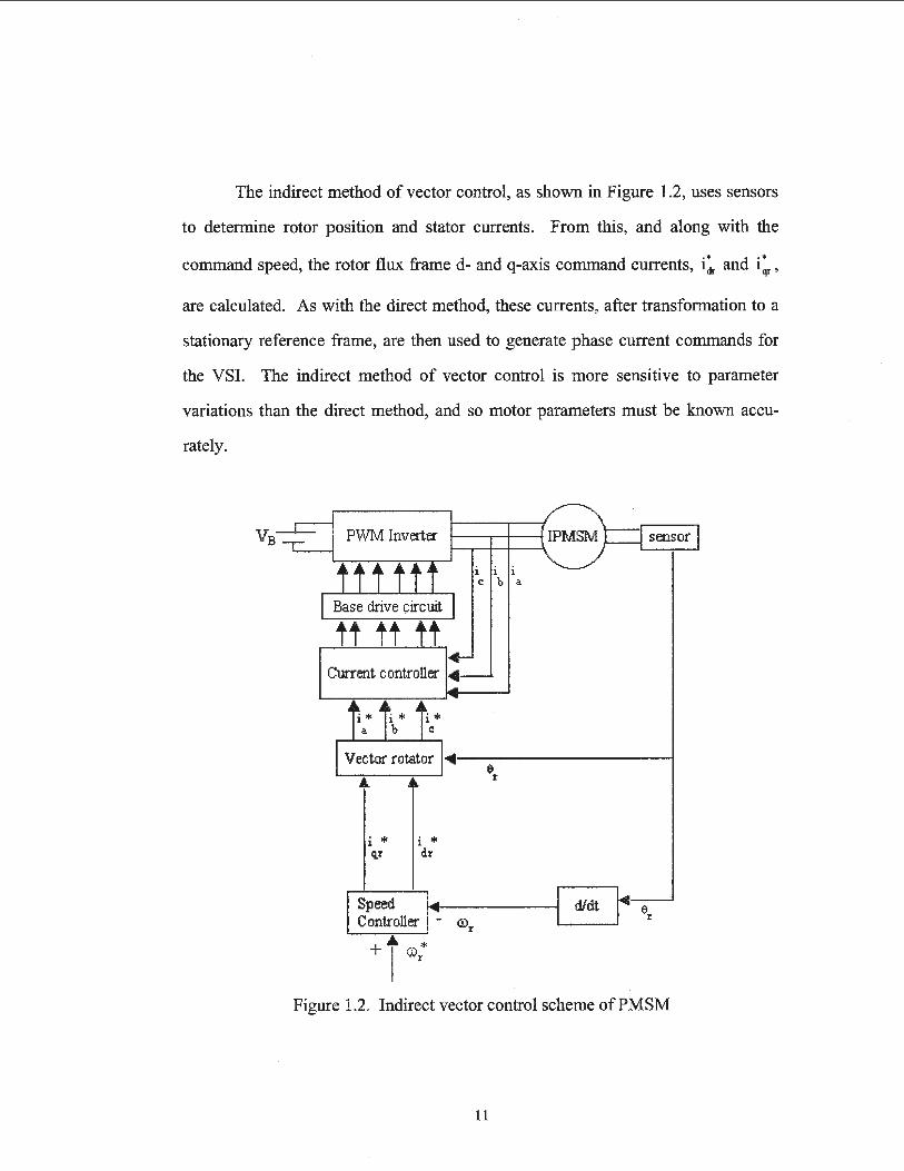
The indirect method of vector control, as shown in Figure 1.2, uses sensors
to determine rotor position and stator currents. From this, and along with the
command speed, the rotor flux frame d- and q-axis command currents, i~ and i:r,
are calculated. As with the direct method, these currents, after transformation to a
stationary reference frame, are then used to generate phase current commands for
the VSI. The indirect method of vector control is more sensitive to parameter
variations than the direct method, and so motor parameters must be known accu-
rately.
PVi!M Inverter
i * i * qr dr
Speed Controller - cor
+ i .,;
i 1 1 c b a
Figure 1.2. Indirect vector control scheme of PMSM
11

In both of these schemes, a current controlled VSI is used to apply the cal
culated command currents to the motor stator. This imposes the need for precise
and accurate control of the VSI, as the current controller has direct influence on the
drive performance. Low-loss current controllers that produce minimal harmonics
and noise in the motor, as well as fast responsiveness for high performance under
dynamic conditions, are required. The performance of various current control
schemes for VSI fed ac and PMSM drives have been investigated [ 1 0-17]. Each
scheme has been shown to have its own unique drawbacks with regards to accuracy
and dynamic response over varying speed ranges. As the purpose of this work is to
investigate improvements in control of the motor itself and not the VSI specifically,
this work employs a simple fixed band hysteresis current control algorithm for the
VSI. This scheme provides fast response and good accuracy in producing a stator
current which tracks the command current within a hysteresis band, while avoiding
unnecessary complexity. The drawback is that the hysteresis controller generates a
random PWM switching pattern, thus producing a switching frequency that varies
over the fundamental period [13].
1.3.2 PMSM Drive Controllers
Modem VLSI and advancing power electronic technologies have lead to the
utilization of microprocessors in the control of the PMSM. This allows the current
advancements in computing power to be applied to PMSM drive control, resulting
in the implementation of complex control strategies. Bose and Szczesny originally
proposed a microcomputer-based control system of an interior perll1anent magnet
synchronous motor (IPMSM) [18].
12

Because of the versatility of the IPMSM, it has become essential to develop
robust controllers for use in high performance drive (HPD) systems. Various un
certainties like sudden changes of command speed, abrupt load changes and pa
rameter variations have to be handled quickly and accurately in such applications.
With this in mind, several types of controllers, including conventional fixed gain
types such as proportional-integral (PI), proportional-integral-derivative (PID) and
pseudo-derivative-feedback (PDF); adaptive types such as model reference adap
tive controllers (MRAC), sliding mode controllers (SMC) and variable structure
controllers (VSC); and intelligent types such as artificial neural network (ANN)
controllers, fuzzy logic controllers (FLC), and neuro-fuzzy controllers have been
used for moderate to high performance drive systems. As my work utilizes the in
direct control of an IPMSM through a current controlled VSI, this is where my lit
erature review will focus.
To date, many researchers have reported their work on the development of
high performance IPMSM drives, with the majority of the control schemes reported
involving the performance of the IPMSM fed by a voltage source or current source
inverter. The reader is referred to the indirect vector control scheme shown in Fig
ure 1.2.
Gummaste and Siemon [19] have proposed a vector control scheme to ana
lyze the steady state performance of a VSI-fed PMSM drive. They also presented a
similar work utilizing the current source inverter fed PMSM drive [20]. For both
schemes they used position feedback control from a shaft position sensor, mounted
on the motor shaft, relaying rotor position back to the microcomputer so that the
inverter could be operated in a self-controlling mode in real time. The constant
torque mode and the constant power mode operations have been investigated, with
13
strategies having been developed for torque control. They have suggested remov
ing the damper winding for the VSI-fed PMSM drive in order to increase operating
stability, as the damper winding provides a path for the flow of harmonic currents
induced for non-sinusoidal voltage outputs of the inverter. However, for the cur
rent source inverter (CSI) -fed PMSM drive system, the damper windings are help
ful in reducing the commutating inductance and, therefore, are not recommended to
be removed.
An analysis of a microprocessor-based implementation of the PMSM drive
has been presented by Liu et. al., [21]. In their work, the motor is fed by the hys
teresis current controlled VSI. To overcome some of the limitations of the hystere
sis controller at low speeds, they have proposed a method utilizing the freewheeling
period. The downfall of this proposal, however, is that this method reduces the av
erage torque delivered by the motor with only modest performance improvements
at low speeds.
Pillay and Krishnan [22-25] have presented a number of papers on model
ing, simulation, analysis and controller design for high performance vector con
trolled PMSM drives using a state space model. They have investigated the tran
sient and steady state performance of the drive using a d-q axis model of the
PMSM, and have also investigated the performances of the hysteresis and ramp
comparator current controllers for the VSI-fed PMSM drive. In these works, a PID
type speed controller, based on the linear model of the PMSM, has been used. This
produces error because, in real time, the PMSM torque does not behave linearly
[26]. Hence, it is very difficult to predict the performance of the drive accurately
using this linear model approximation. In addition, the inherent nature of the PID
speed controller makes drive performance very parameter and load sensitive. Pillay
14

and Krishnan have not reported drive performances over wide speed ranges, but
rather only for certain command speeds.
In other work, Pillay et. al., [27] have proposed a control scheme for a
PMSM based on dual digital signal processors (DSP). One DSP is used to imple
ment the current controller algorithm and the other the vector control algorithm.
The performance of this drive is diminished due to the slower speed of the DSPs
employed; and their use of a look-up table in generating command currents may not
be suitable for a wide range of speed operations. Therefore, there is a lack of ro
bustness with this drive, and comprehensive test results at different dynamic oper
ating conditions have not been reported. However, the experimental results do
show the effectiveness of the controller and its potential.
B.K. Bose (28] has presented a high performance inverter-fed IPMSM drive
system using a closed-loop torque control scheme in which command torque is de
termined using feedback and taking into accounts the effects of saturation, tempera
ture variation and non-linearity. The drive system has been incorporated in the
constant torque as well as constant power regions. However, the performance of
this drive system has been reported only for a fixed speed, and testing of the drive
over a wide speed range and at different dynamic operating conditions is necessary
to establish the efficacy of the drive.
An adaptive current control scheme for the PMSM drive has been proposed
by Huy and Dessiant [29]. Their controller uses two modes, a hysteresis current
control scheme for transient operation and a predictive current control scheme for
steady state operation. The performance of this drive at low operating speeds has
not been reported.
15

Huy et. al., [30] have presented an analysis and implementation of a real
time predictive current controller for a PMSM synchronous motor servo drive. Al
though a high performance standard has been obtained with this controller, its im
plementation requires hardware incorporating an EPROM-based approach, making
this scheme less flexible than the microprocessor-based approach.
Bose and Szczesny [31] have proposed a microcontroller-based controller
of an IPMSM drive for electric vehicle propulsion. The control system incorpo
rates both the constant torque region as well as the constant power region where the
flux weakening mode of operation is used. This drive system has been imple
mented on a multiprocessor architecture, making the overall system costly.
Jahns et. al., [32] reported an adjustable speed drive using a torque control
technique for an IPMSM by providing control of the magnitude and phase angle of
the sinusoidal phase currents with respect to the rotor orientation. This method
cannot provide a smooth transition from the constant torque mode to the constant
power mode while the motor is in operation. In addition, the performance of this
drive system has not been investigated over a wide speed range.
Jahns (33] also proposed a flux-weakening mode operating scheme for the
IPMSM. This allows for investigation of the performance of the drive over an ex
tended speed range. In this method, the d-axis rotor current is obtained from the
sensed stator phase currents and the d-axis command current.
Likewise, Morimoto et. al., [34-39] have proposed a flux-weakening mode
based controller for an IPMSM drive. In this work, the magnetic saturation and
demagnetization effects of permanent magnets has been accounted and compen
sated for. This results in high torque and high efficiency operation within the
maximum voltage and current limit ratings of the inverter and the motor. Different
16

control methods, such as as id = 0, unity power factor and constant flux linkage
schemes have been investigated, and a comparison of the various methods has been
made over a wide speed range. Regarding the magnitude and phase errors inherent
when using a current controlled VSI, a compensating technique based on a calcu
lated value of q-axis inductance, Lq, from the actual q-axis current has been used.
Then, in order to overcome saturation, the d-axis command current is generated
from the calculated value of Lq. The shortcoming of this work is that the effects of
parameter variations due to noise, temperature, etc. are not considered.
Rahman et. al. [40] have proposed a flux-weakening mode based torque
controller for the IPMSM drive for operation exceeding base speed. Maximum
voltage and current capabilities of the motor and the inverter during operation are
also accounted for in this work. The drive has not been tested for variable speed
operation.
Vaez et. al. [ 41] have proposed a vector control strategy of the IPMSM
drive aimed at producing minimum loss operation. They have used a PI-based
speed controller, making this scheme sensitive to parameter variations, load
changes, etc ..
Radwan et. al. [42] have developed a hybrid current controller for the
IPMSM drive which incorporates a ramp comparator controller for low speed op
eration and a hysteresis current controller for high speed operation. This controller
produces stable operation over a wide speed range. However, as with Vaez et. al.
the speed controller is PI-based.
Hoque et. al. [43] have reported a vector control strategy of the IPMSM
drive based on the maximum torque per ampere (MTPA) scheme. In this work, d
axis command current is obtained from q-axis command current by use of a Taylor
17

series expansion to overcome mathematical difficulties arising from nonlinearities
of the model. A PI-based speed controller has been used. This work was done in
conjunction with the work presented in this thesis.
Other works [44-47] investigating PMSM drive performance while in flux
weakening mode have been reported. Most of these works are based on conven
tional PI and PID based speed controllers. These controllers offer the advantages
of simplicity and ease of implementation in real time. However, they are very sen
sitive to parameter variations due to load changes, sudden changes of command
speed, saturation, temperature variations and other system uncertainties. Therefore,
it is difficult to tune the controller parameters precisely for an optimal implementa
tion. Consequently, these types of controllers are not suitable for high performance
applications, and researchers have been prompted to develop adaptive control
schemes for PMSM drive systems in which the controller parameters can be
adapted in real time in response to system parameter variations and load changes.
1.3.3 PMSM Drives with Adaptive Controllers
To date, adaptive controllers have been used in PMSM drives to achieve
fast transient responses, parameter insensitivity, nonlinear load handling capabili
ties and high adaptabilities to other types of uncertainties.
The model reference adaptive controller (MRAC) is one such scheme in
which the drive forces the motor response to follow the output of a reference model
regardless of drive parameter changes. A MRAC may be used with a PI controller
to adapt the controller parameters compensatively for system parameter changes.
18

Parameters are adapted by trial and error such that the error between the actual and
the desired responses remains within specified limits.
Choy et. al., [ 48] have proposed a vector control position servo PMSM
drive system using a MRAC. In their work a MRAC is used to reactively tune a PI
controller. The steady state error gain component of the PI controller is used to
compensate the chattering problem that occurs due to discontinuous control inputs.
However, this drive still does not completely overcome the chattering problem.
Cerruto et. al., [ 49] have proposed a MRAC-based PMSM drive for robotic
applications. A MRAC has been used to compensate for changes in system pa
rameters such as inertia and torque constant. As explained previously, the error
between the reference model speed and the actual speed is used to adjust the pa
rameters. The shortcoming of this model is the computational burden that the algo
rithm imposes on the microcomputer. This limits the maximum operating speed of
the drive.
Sozer and Torrey [50] have proposed a MRAC-based PMSM drive utilizing
an adaptive flux weakening mode controller that adjusts the d-axis current id com
pensatively. However, this drive has been reported in simulation only and has not
been tested at variable speed conditions.
MRAC is only one of several types of adaptive controllers. Other popular
schemes that have been used in PMSM drive systems are the sliding mode control
ler (SMC) and the variable structure controller (VSC).
Namudri and Sen [51] have presented a SMC-based vector control system
of a synchronous motor drive for a position servo drive. In their work a gate turn
off (GTO) inverter and phase-controlled chopper are used to provide the torque
19

producing current component. The controller accommodates parameter variations
and load changes.
Consoli and Antonio [52] have proposed a DSP-based vector control
scheme for an IPMSM drive using a SMC for torque control. In this work, both the
actual motor currents and terminal voltages are used as feedback signals to generate
the torque and flux for flux-weakening mode operation above base speed. The ef
fects of constant acceleration, constant speed and constant deceleration have been
accounted for in the design of the SMC. However, this drive system has been pre
sented in simulation only and not in real-time where the parameter variations are
not defined.
An ac servo drive using a variable structure controller (VSC) for position
and speed control of a PMSM has been presented by Ghirby and Le-Huy [53].
Two control loops have been used, an inner loop for predictive current controllers
and an outer loop for a position or speed controller. The performance of the drive
has not been reported for wide variable speed operations, and suffers somewhat
from chattering.
Sepe and Lang [54] have also proposed an adaptive speed controller for the
PMSM drive system in which the mechanical parameters of the motor have been
estimated in real-time to continually tune the gain of the controller. As with Ghirby
and Le-Huy, the system is composed of two loops: An inner loop consisting of the
motor, inverter, current controller, speed controller and filter; and a slower, outer
loop consisting of a motor parameter estimator and the control algorithm for the
controller. This system has been implemented on a microprocessor of limited
computational capacity, therefore the performance of the drive is impaired by sig
nificant noise in steady state operation.
20
Clearly, compared to conventional fixed-gain PI and PID controllers, adap
tive controllers show improved performance because of their relative insensitivities
to parameter variations, load changes and other uncertainties. However, all of this
is achieved at the cost of increased computational burden, hence reducing practical
ity for real-time implementation. And almost all of the adaptive controller-based
systems suffer from chattering, overreaching and steady state errors due to finite
switching. In addition, the unavailability of the exact system parameter model
makes for cumbersome design approaches for these types of controllers.
1.3.4 PMSM Drives with Intelligent Controllers
To solve some of the problems associated with fixed gain PI, PID and vari
ous adaptive controllers, recent researchers have investigated intelligent controllers
such as artificial neural network (ANN), fuzzy logic (FL), neuro-fuzzy (NF), and
genetic controller-based systems. These controllers are self-adaptive and do not
need any advance information about system nonlinearities. They are often called
artificial intelligence (AI) controllers, because they involve software programming
where the computer mimics human thinking in the control of the motor.
ANNs have been reported for use in controllers for PMSM drives. El
Sarkawi et. al., [55] have proposed one such scheme for a high performance brush
less de motor drive. In their work, a MRAC is used to implement a multi-layer
ANN. The inputs of the ANN are the estimated speed from the reference model,
three consecutive past samples of actual speed, a past sample of the converter input
voltage, and the error between the reference model speed and the actual speed. A
back-propagation algorithm is used to train the network. However, the speed con-
21

trol of this drive is not precise because the ANN must be trained offline. This
shortcoming may render the drive incapable of effectively handling different dy
namic operating conditions such as load changes, parameter variations and system
disturbances.
Similarly, Shigou et. al., [56] have proposed an offline-trained ANN-based
controller for a brushless de servo motor drive system. In their work, they have
used an analog speed controller in order to obtain better servo performance. How
ever, they still have not produced satisfactorily precise speed control.
Rahman and Hoque [57] have presented an online ANN-based PMSM drive
system utilizing a back-propagation training algorithm and combined offline and
online training. There are two artificial neural networks: One to generate the
command signal and the other to generate the estimated signal. Controller parame
ters are then updated in accordance with the error between the two signals. In this
work, however, the d-axis command current, ict *, is assumed to be zero, which
makes it impossible to control the motor above base speed.
Another work, by Y. Yi et. al. [58] has utilized an ANN-based controller for
an IPMSM. This work shows encouraging results, but, as with other ANN-based
systems, simulation and experimental results show room for improvement in terms
of disturbance rejection such as insensitivity to load variations, parameter varia
tions, etc ..
Hoque et. al. [59] have reported a similar online ANN-based PMSM drive
system using the maximum torque per ampere (MTP A) scheme. Once again, a
back-propagation training algorithm making use of combined offline and online
training is used, but in this work, d-axis command current is obtained from q-axis
command current by use of a Taylor series expansion. This is done to overcome
22

mathematical difficulties arising from the nonlinearities of the model. The ANN
tunes the parameters of a PI-based speed controller. This work was done in con
junction with the work presented in this thesis.
Recently, researchers have developed fuzzy logic controllers (FLC), show
ing encouraging performances, for use in PMSM drives. In almost all cases the
FLC has been used as a speed controller.
Inoue et. al., [60] have presented a fuzzy algorithm for the brushless de
servo motor drive. The fuzzy algorithm is used to tune the gain of the PI controller
in response to load changes, parameter changes and system disturbances. The ac
tual speed, reference speed and output of the reference filter are used to generate
the membership functions. The experimental results show optimum response after
several auto-tuning calculations. However, as the drive system incorporates a ref
erence generator, somewhat complex fuzzy calculations and two PI controllers, the
system imposes high computational burden, thus diminishing performance.
Erenay et. al., [61] have proposed a fuzzy logic approach for the brushless
de motor drives used in washing machines. They have made a comparison among
various controller techniques namely, conventional PI, fuzzy PI, fuzzy reset rate
and fuzzy gain scheduled Pl. However, they have investigated the speed responses
only for fixed speed conditions. Moreover, because of the large number of fuzzy
rules incorporated, high computational burden may render these FLC-based sys
tems incapable of high-speed operations. In experimental results, it is shown that
the motor cannot follow the command speed smoothly.
A fuzzy logic-based MRAC for the PMSM drive has been proposed by
Koviac et. al. [62]. Simulation results verify the effectiveness of the proposed al-
23

gorithm, which was designed using the linearized model of the PMSM (the refer
ence model being parameter dependent). This may not translate to real-time im
plementation where nonlinear load changes and parameter variations exist with dif
ferent operating conditions.
Uddin and Rahman [63] have presented a FLC-based vector control scheme
for the IPMSM. Their work uses a fuzzy algorithm to determine q-axis command
current from the error between actual and reference speeds, and the difference be
tween the current and previous speed errors. D-axis command current is set to be
zero as a simplifying approximation. Heavy computational burden and the inaccu-
racy of the i~ = 0 approximation limit the capacity of this scheme.
The application of fuzzy logic for IPMSM drives is in its initial stages. The
heavy computational burden imposed by fuzzy algorithms limit these systems to
implementation with only the fastest, most resource intensive microprocessors.
Therefore, there exists a need to reduce the complexity of these algorithms so they
may be implemented more economically. Furthermore, because of mathematical
complexity and nonlinearity, the maximum torque per ampere approach for PMSM
drives has not been practically implemented. Without this scheme PMSM drives
must operate at less than optimum efficiency. Simplified FLC-based controllers,
combined with MTP A mode operation, can overcome various drive uncertainties
such as unknown nonlinear load characteristics, parameter changes and other sys
tem disturbances, as well as provide maximum efficiency operation of the PMSM
at and below the rated speed.
24

1.4 Problem Identification and Thesis Objectives
High performance drive (HPD) systems must provide fast and accurate
speed responses, quick recoveries of reference speed from sudden disturbances of
all natures, and show insensitivity to parameter variations. Each of the systems
presented to date have shortcomings that require remedy if the IPMSM is to be
practically implemented under HPD standards. Thus, it is necessary to further de
velop control algorithms and approaches to produce this high standard of perform
ance in a practical manner.
While the IPMSM has many advantages over conventional motors, its op
eration is strongly affected by motor magnetic saliency, saturation and armature
reaction effects [64]. Particularly, the saturation of the iron portion of the rotor
around the permanent magnets produces a distortion of the air-gap flux that affects
the reactance parameters of the motor. These reactance changes with different op
erating conditions and, hence, affect the performance of the drive system if they are
not accounted for. This makes the control of the IPMSM for HPD applications an
engineering challenge.
The objective of this work is to develop and implement a complete IPMSM
drive system to be used in HPD applications. The vector control scheme, incorpo
rating a speed controller and a current controller is used because it decouples the
torque and flux, thus providing faster transient responses and making the control
task easier. An efficient speed controller, incorporating heretofore undeveloped
methods is presented for the high performance IPMSM drive.
As discussed in the literature survey, fixed-gain proportional integral (PI)
and proportional integral derivative (PID) controllers, model reference adaptive
controllers (MRAC), variable structure controllers (VSC), sliding mode controllers
25

(SMC) and self-tuning regulators (STR) all require the accurate and precise knowl
edge of system model parameters. Moreover, the fixed-gain PI and PID controllers
are especially sensitive to parameter variations, load changes and other system dis
turbances. Intelligent controllers, such as the fuzzy logic controller (FLC), do not
need any information about the system mathematical model, are self-adaptive to
uncertainties and can handle any kind of system non-linearity. However, FLC
based drive systems incorporate complex algorithms that impose such computa
tional burdens that they can only be incorporated by making performance compro
mises or by use of the latest, most powerful personal computer systems. Therefore,
a large part of the purpose of this work is not only the real-time implementation of
the IPMSM drive incorporating an intelligent, FLC-based controller, but also to
achieve this control with minimal complexity and computational burden. In addi
tion, many researchers have simplified the non-linear model of the IPMSM to a lin
ear one by forcing the d-axis cmTent to zero (i.e. id = 0). This is not accurate and,
as a result, produces a motor control that requires increased stator current to pro
duce a given torque. This work includes the development of a practical implemen
tation of the maximum torque per ampere (MTPA) scheme with the real case of id -:f:.
0, which produces motor torque with the minimum possible stator currents.
Laboratory implementation has been carried out to verify theoretical and
experimental results. These results have been compared with those obtained using
a traditional FLC-based system with~ = 0.
26

1.5 Thesis Organization
This thesis consists of six chapters. The introduction and literature survey
of vector control techniques for permanent magnet synchronous motor drives, as
well as the objectives of this thesis have been covered in this chapter.
Chapter two contains the theoretical development of the mathematical
model of the interior permanent magnet synchronous motor (IPMSM) and presents
the theoretical development of the analysis and modeling of the PWM VSI-fed
IPMSM drive with maximum torque per ampere (MTP A) based control.
Chapter three outlines the development of the fuzzy logic based speed con
troller for the IPMSM drive and presents a simplified fuzzy logic based speed con
troller incorporating the maximum torque per ampere mode of operation that re
duces complexity and computational burden. Ideas developed include linguistic
variables, membership functions, fuzzification, rule evaluation and defuzzification.
Both controllers are incorporated into problem specific vector control schemes for
theiPMSM.
Chapter four presents the simulation results of both of these drives.
Chapter five contains the results of the real-time experimental implementa
tion of the simplified FLC/MTPA drive which has been implemented using a digi
tal signal processor (DSP) based vector control of a laboratory 1 hp IPMSM.
Chapter 6 presents the summary of the contribution of this work and the
conclusion.
Finally all pertinent references are listed.
27
Chapter 2
Analysis and Modeling of the PWM
VSI-Fed IPMSM Drive
2.1 General Introduction
This chapter presents the development of the mathematical model of a com
plete current-controlled voltage source inverter (VSI) -fed interior permanent mag
net synchronous motor (IPMSM) drive using the d-q axis model of the IPMSM. A
fixed-band hysteresis current controller has been used to apply the correct stator
currents to the motor through the VSI.
In order to operate the vector control scheme, a fuzzy logic based speed
controller is used. This will be developed in chapter 3.
28

2.1.1 Mathematical Modeling of the IPMSM
The IPMSM is similar to the conventional synchronous motor with the ex
ception that the field excitation is provided by permanent magnets instead of a
wire-wound de rotor field. Because of this, the mathematical model ofthe IPMSM
can be derived from the standard model of the synchronous motor by removing the
equation related to the field current and other associated terms.
The flux linkages in the three stator phase windings due to the permanent
magnets of the rotor are given in matrix form as [65]:
l~= J
sin er
sin( er-231t) \jl bm = \jl m (2.1)
\jl em
sin( er + 231t)
The three phase air gap flux linkage equations are given in matrix form as:
sin er
sin( er 231t) (2.2)
sin( er + 231t)
where ia, ib, ie are the three phase currents, Laa, Lbb, Lee are the self inductances and
Mab, Mbe, Mea are the mutual inductances, respectively, \jim is the constant flux sup:..
29

plied by the permanent magnets and 8r is the rotor position angle. Rotor position
angle 8r is defmed as,
(2.3)
The voltage equations of the three phases of the IPMSM can be defined as,
. d\jf a Va = rala + - -
dt (2.4)
(2.5)
- . d\jf c Vc-fclc + --
dt (2.6)
where Va, vb, Vc are the three phase voltages and ra, rb, rc are the three stator phase
resistances. In matrix form, this is,
(2.7)
where p is the time differential operator, ~. Inspection of Eqn. (2.2) reveals that dt
the flux linkages are functions of rotor position and, therefore, functions of rotor
speed. This means that the coefficients of the voltage equations are time varying
(except, of course, when the motor is stationary). In order to avoid the complexity
30

of calculations, all of the equations can be transformed to the synchronously rotat-
ing rotor reference frame where the machine equations are no longer dependent on
the rotor position. This is accomplished using Park's transformation equations
[65]. First, the machine equations are transformed from the stationary a-b-c frame
to the stationary d-q frame, then they are transformed from the stationary d-q frame
to the synchronously rotating dr-qr frame. Using x to represent the machine phase
variables, the inverse Park's transform gives,
Cos8r
co{ er-231t) (2.8)
co{ er + 231t)
The corresponding Park transform is,
Cos8r co{ Sr 2
3n) co{ er + 231t)
[:J~ [:J Sin Sr Sin(er 237t) Sin( Sr +
23n) (2.9)
1 1 1 -2 2 2
where Xo is the zero sequence component. The matrix element x may represent ei-
ther voltage or current. Eqns. (2.8 -2.9) are both in a stationary reference frame, so
Sr is only the initial rotor position Sr(O) which is also the angle difference between
31

the q-axis and a-phase. For balanced 3-phase, Xo does not exist and it is also con-
venient to set Sr(O) = 0 so that the q-axis coincides with the a-phase. Under these
conditions, Eqns. (2.8) and (2.9) become,
and
0
-../3 2
.J3 2 2
-1
3 -1
.J3
[ ::] (2.10)
(2.11)
To convert these variables to the rotating d-q frame we use Fig 2.1 as refer
ence. From this, we see that the quantities in the stationary d-q frame can be con
verted to the synchronously rotating frame as follows:
(2.12)
The inverse relation can be written as,
32

Sin8r ] [X~ ] Cos8r x~
(2.13)
Now, using equations (2.7)-(2.8) and (2.13) the d r_q r model of the IPMSM
can be written as,
(2.14)
(2.15)
where vi and Vqr are the d and q axis voltages, il and iqr are the d and q axis cur
rents, respectively, rs is the per phase stator resistance and ills is the stator fre-
quency.
e.= ro.t
o-axis
d'-~~ d-axis
Fig. 2.1 Relative positions of stationary d-q axes and rotating dr -qr axes.
33

The following assumptions have, thus far, been made:
(a) The eddy current and hysteresis losses are negligible.
(b) There is no squirrel cage on the rotor side.
(c) The induced emf is sinusoidal.
(d) The saturation is neglected.
(e) There are no field current dynamics or magnet imperfections.
(f) The stator resistances of the three phases are balanced.
The q-axis flux linkage 'l' ~ and the d-axis flux linkage 'I'~ can be written as,
where,
Lq = Lt + Lmq
Ld = Lt + Lmd
(2.16)
(2.17)
(2.18)
(2.19)
Ld and Lq are the d and q axis inductances, Lmd and Lmq are the d- and q-axis mag
netizing inductances, respectively, and Lt is the leakage inductance per phase. The
stator frequency ros is related to the rotor frequency ror as,
(2.20)
34
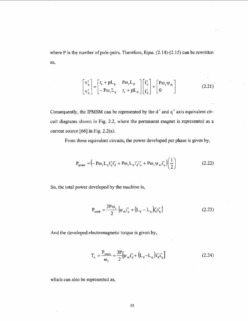
where Pis the number of pole-pairs. Therefore, Eqns. (2.14)-(2.15) can be rewritten
as,
(2.21)
Consequently, the IPMSM can be represented by the d rand q r axis equivalent cir
cuit diagrams shown in Fig. 2.2, where the permanent magnet is represented as a
current source [66] in Fig. 2.2(a).
From these equivalent circuits, the power developed per phase is given by,
(2.22)
So, the total power developed by the machine is,
(2.23)
And the developed electromagnetic torque is given by,
(2.24)
which can also be represented as,
35

(2.25)
where T L is the load torque, P is number of pole pairs of the motor, p is the differ
ential operator, Bm is the friction damping coefficient and Jm is the rotor inertia
constant.
. r
r r Vd
. r lq r
1 V r
g
Lmd
(a)
(b)
Fig. 2.2. Equivalent circuit model of the IPMSM: (a) d-axis, (b) q-axis.
36

So, finally, the IPMSM model equations may be expressed as follows:
piqr = (vqr- R iqr -Pror Lct ictr- Pror 'I'm)/ Lq
pii =(vi-R ii +Pror Lq iq)/ Lct
(2.26)
(2.27)
(2.28)
The above three fundamental equations are used to model the IPMSM. The spe-
cific motor parameters used for simulation are given in Appendix A.
2.2 Vector Control of the IPMSM Drive
From equation (2.24) one obtains the expression of torque,
(2.29)
we see that the second term in the electrical torque equation (2.29) represents a
complex interaction of inductances, Lct and Lq and also the currents, i/ and iqr·
However, in the case of the IPMSM, Lq is larger than Lct, and both undergo signifi
cant variations under different steady state and dynamic loading conditions [64].
So the complexity of the control of the IPMSM drive arises due to the nonlinear
nature of the torque Eqn. (2.29).
Using phasor notations, and taking the dr axis as reference, the steady state
phase voltage Va can be derived from the steady stated r_q r axis voltages described
in Eqn. (2.21) as,
37
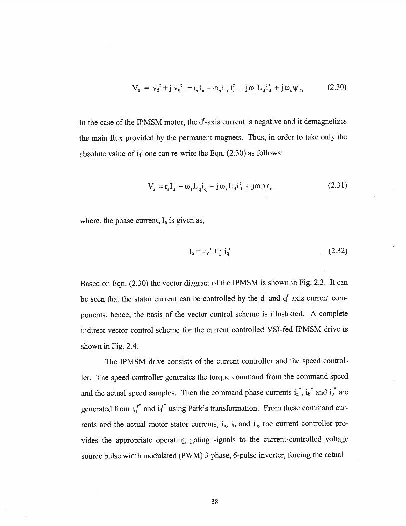
(2.30)
In the case of the IPMSM motor, the dr-axis current is negative and it demagnetizes
the main flux provided by the permanent magnets. Thus, in order to take only the
absolute value of ictr one can re-write the Eqn. (2.30) as follows:
where, the phase current, Ia is given as,
I · r · · r a= -ld + J lq
(2.31)
(2.32)
Based on Eqn. (2.30) the vector diagram of the IPMSM is shown in Fig. 2.3. It can
be seen that the stator current can be controlled by the dr and qr axis current com
ponents, hence, the basis of the vector control scheme is illustrated. A complete
indirect vector control scheme for the current controlled VSI-fed IPMSM drive is
shown in Fig. 2.4.
The IPMSM drive consists of the current controller and the speed control
ler. The speed controller generates the torque command from the command speed
and the actual speed samples. Then the command phase currents ia *, ib * and ic * are
generated from iq r* and it using Park's transformation. From these command cur
rents and the actual motor stator currents, ia, ib and ic, the current controller pro-
vides the appropriate operating gating signals to the current-controlled voltage
source pulse width modulated (PWM) 3-phase, 6-pulse inverter, forcing the actual
38

qr-axis
V a -ro. Lqiq
Iars
·· ... ···· ...
~---------~!11::::.------.....::;ii~--_;)~ dr-axis ictr
'I'm
Fig. 2.3. Vector diagram ofiPMSM parameters.
Speed i:loo. (\,_. -Controlle ~-------;
+i ~·
6
&&rl--r--~--------------~
Fig. 2.4. Block diagram of complete current-controlled VSI-fed IPMSM drive.
39

motor currents to follow the command currents as closely as possible and, hence,
forcing the motor to follow the command speed by feedback control.
Therefore, in order to operate the motor in a vector control scheme the
feedback quantities will be the rotor angular position and the actual motor currents.
2.2.1 Maximum Torque Per Ampere Speed Controller
The speed controller generates the torque command from the command
speed and the actual speed samples. Traditionally, this has been accomplished by
use of PI and PID controllers. However, these controllers produce unsatisfactory
performance for high performance drive systems, so alternatives must be found (as
covered in Chapter 1 ). In this work, Fuzzy Logic Controllers have been used to
design the speed controllers. Their development will be detailed in Chapter 3.
In addition, the d-q axis command currents, 4tr* and it are determined from
command torque by manipulation of Eqn. (2.29). One of the main problems asso
ciated with the control of the IPMSM is the non-linearity arising out of the devel
oped torque, as can be seen from the torque equation (2.29). Many researchers
have focused their attention on the vector control of the IPMSM drive by forcing
id = 0, which linearizes the torque equation [25, 28, 32, 34]. However, in real-
time the electromagnetic torque truly is non-linear in nature. In order to incorpo
rate this non-linearity in a practical IPMSM drive, a control technique known as
maximum torque per ampere (MTPA) has been derived which provides maximum
motor torque with minimum stator current [25, 28, 32, 40, 67]. This MTP A strat
egy is very important from the limitation of IPMSM and inverter rating
points of view, which optimizes the drive efficiency. Figure 2.5 shows the
40

maximum torque per ampere trajectory that provides information for the con-
trol strategy.
The problem associated MTPA control technique is that its implemen
tation in real time becomes complicated because of the complex relationship
between d-axis and q-axis currents. Some researchers have solved this prob
lem by use of look-up tables, based on this trajectory, ford- and q-axis cur-
rents [40, 43].
• • 5 .......... ...... ,. ................... . .. .. ·· ···· .· ................ .-.. .......... ........... .
~ Maximum Torque/Ampere trajjory f .. .. . .... .. L. ........ . Qi 4 •• • ••••o•o •o• o•o•o•o o o O o o oo ' 0 0 H 0
Q. E C'CI
. .... i .... . i . ...... },, .. . . .. ... . . .. ) ... . . . .... .. ; ...... ............. ....... .
. . . ... . . . . . . · l .. . .. . . . . . . . . . .. . . . . . .
QL---J-__ _L __ _J ____ L_ __ ~ __ _L __ _J ____ L_ __ ~--~
-5 -4.5 -4 -3.5 -3 -2.5 -2 -1 .5 -1 -0.5 0 d-axis current, ampere
Fig. 2.5. Maximum torque per ampere (MTPA) trajectory on constant torque loci.
41

For application of the MTP A technique, the relation between ici and iq can be
obtained by differentiating Eqn. (2.29) with respect to iq and setting the resulting
expression to zero. The relation between ict, iq and Ia can be derived from Eqn.
(2.32) as
Giving,
(2.33)
d~ =3p['l! +(Ld-L )id-(Ld-L )i 2 ~]=0, (2.34)
dz 2 m q q q 12 -iz q a q
• 2 l
If! +(L -L )i - (L -L )!L=o. (2.35) m d qd d qi
d
Rearranging the order ofLct and Lq and solving for ict gives,
lf/rn (2.36)
Substituting Eqn. (2.36) into Eqn. (2.29), one can get a non-linear relationship
between iq and T e as,
42

(2.37)
Because of the square root terms, the real-time implementation of the drive
system becomes difficult using Eqns. (2.36) and (2.3 7). This work presents a
simplified relationship between the d-q axis currents, which is obtained by
expanding the square root term of Eqn. (2.36) using a Taylor series expansion
around a point approaching zero. (Zero itself was not used because, practically, it
is desired to have the approximation most accurate for small values of iq but not
exactly zero.) Substituting the appropriate experimental machine parameters given
in Appendix A into Eqn. (2.36) gives,
id = 4.22839 - ~17 .87925 (2.38)
and expanding Eqn. (2.38) in a Taylor series about iq = 0.001 gives,
id =-0.11825(iq -0.001) 2 - 0.00024(iq -0.001)-0.118xl0 -6 (2.39)
Substituting Eqn. (2.39) into Eqn. (2.29) and solving for iq gives,
iq =- 0.000047 (Te - 0.000942 ) 2 + 1.06157 (Te - 0.000942) + 0.001 (2.40)
43

Equations (2.39) and (2.40) are used in the speed controller to determine the
rotating frame d-q axis command currents for the MTP A control of the IPMSM.
2.2.2 Vector Rotator
The command current outputs of the speed controller are in the rotating ro
tor reference frame. Therefore, they must be transferred to the stator reference
frame. The inputs of the vector rotator block are the d-q axis command currents,
i/ and it, from the speed controller and the rotor position 9r from the sensor on
the motor. The outputs are the three phase command currents ia"', ib * and ic *.
The transformation is done by first converting the synchronously rotating dr
- qr axis quantities to the stationary d-q axis quantities and then transforming these
stationary d-q axis quantities into the corresponding a-b-c phase currents.
2.2.3 Current Controller and Voltage Source Inverter
Once the appropriate a-b-c phase command currents are generated by the
vector rotator a current controller is used to control the voltage source inverter
(VSI) to produce these command currents on the motor stator. The outputs of the
current controller are the firing pulses for the inverter switches. Therefore, the VSI
forces the motor to follow the command speed by feedback control.
The current control principle for the VSI used in this work is the based on
the fixed-band hysteresis controller. The hysteresis current controller is most
commonly used for high performance drive applications because of its simplicity
and ease of implementation while providing acceptable results.
44

2.3 Current Control of the Voltage Source Inverter
The purpose of the current controller is to force the motor stator currents to
follow the a-b-c phase command currents as closely as possible. These command
currents are produced from the error between the command speed and samples of
the actual speed of the motor with the intent of producing a motor speed identical to
that of the command speed. Therefore, under the scheme of speed control, the cur
rent controller forces the motor to follow the command speed.
The current-controlled VSI operation can be described, with reference to Fig.
2.6, as follows: The errors between the actual motor currents and the command
currents are processed by the hysteresis current controller to generate the firing
pulses for the transistors of the inverter. Each stator phase of the motor is
NA NB NC
Fig. 2.6. Current controlled voltage source inverter for the IPMSM drive.
45
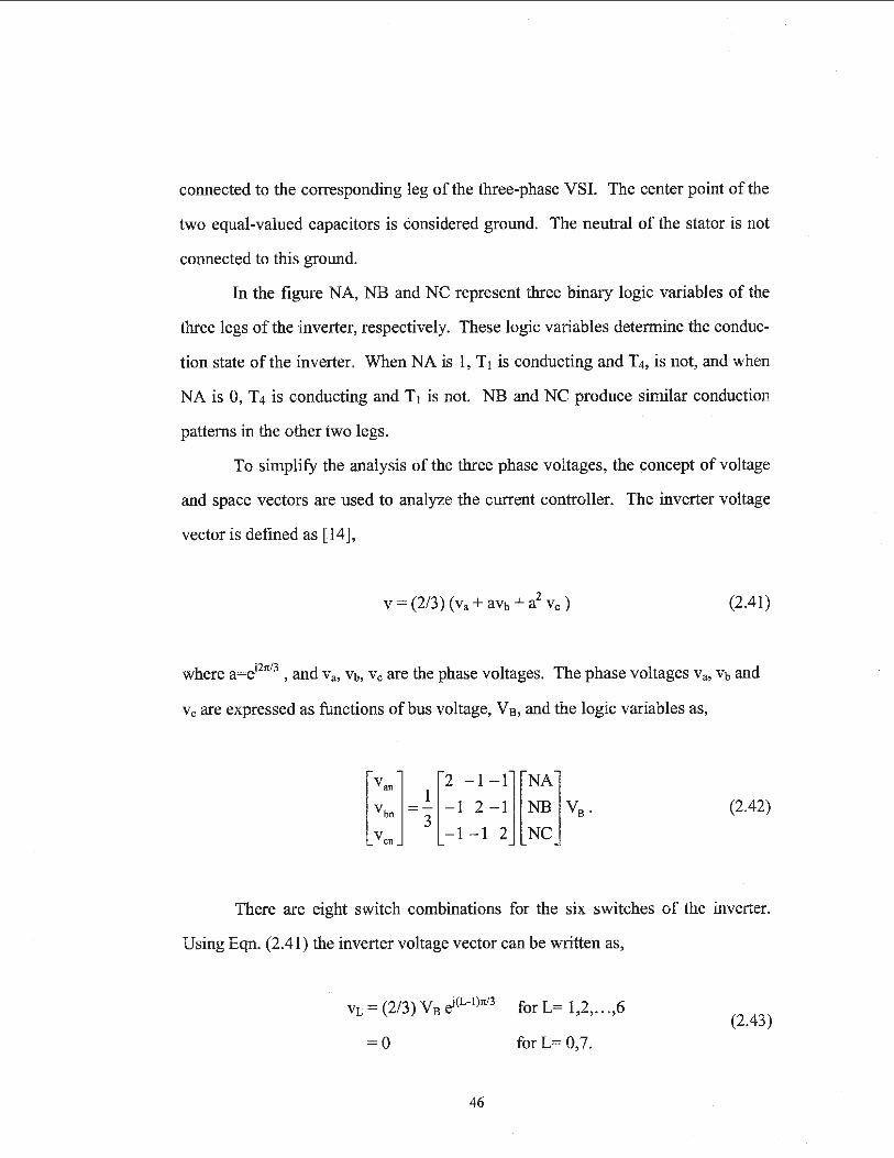
connected to the corresponding leg of the three-phase VSI. The center point of the
two equal-valued capacitors is considered ground. The neutral of the stator is not
connected to this ground.
In the figure NA, NB and NC represent three binary logic variables of the
three legs of the inverter, respectively. These logic variables determine the conduc
tion state of the inverter. When NA is 1, T1 is conducting and T4, is not, and when
NA is 0, T4 is conducting and T1 is not. NB and NC produce similar conduction
patterns in the other two legs.
To simplify the analysis of the three phase voltages, the concept of voltage ·
and space vectors are used to analyze the current controller. The inverter voltage
vector is defined as [14],
v = (2/3) ( Va + avb + a2 v c ) (2.41)
where a=d21t13, and Va, Vb, Vc are the phase voltages. The phase voltages Va, Vb and
Vc are expressed as functions ofbus voltage, Vs, and the logic variables as,
lv ] l2 -1 -1] lNA] v:: = k - 1 2 -1 NB V8 .
v -1 -1 2 NC en
(2.42)
There are eight switch combinations for the six switches of the inverter.
Using Eqn. (2.41) the inverter voltage vector can be written as,
VL = (2/3) Vs ei<L-J)1tt3 for L= 1,2, ... ,6 (2.43)
= 0 forL= 0,7.
46

The logic operation ofthe current-controlled VSI is summarized in Table 2.1.
The voltage vectors corresponding to the six active states are shown in Fig.
2.7. The magnitude of each voltage vector is (2/3)Va. The magnitudes of the volt-
Table 2.1. Conduction modes of the VSI under current control
Leg 'a' Leg 'b' Leg ' c' Voltage
State, L Tt T4 T3 T6 Ts T2 Operating modes phasor
0 0 1 0 1 0 1 Freewheeling Yo
1 1 0 0 1 0 1 Active VI
2 0 1 1 0 0 1 Active v2
3 I 0 1 0 0 1 Active v3
4 0 1 0 1 1 0 Active V4
5 1 0 0 1 I 0 Active Vs
6 0 1 1 0 1 0 Active v6
7 1 0 1 0 1 0 Freewheeling V7
2
Fig. 2. 7. VSI voltage vectors.
47

age vectors corresponding to the freewheeling states, V0 and V7, are zero. In these
cases, no voltage is applied to the motor because in these states no conduction path
exists across any leg ofthe inverter.
2.3.1 Effect of Unconnected Neutrals
If the neutral of the motor stator is not connected to the de bus midpoint, the
switching of any one phase depends on the states of the other two phases. This
means that the individual line-to-neutral voltages are dependent on each other and
each line current will depend not only on the corresponding inverter phase but also
on the state of the other two phases. Therefore, the current controller experiences
interaction between the phases of the inverter, and the actual current potentially
may not follow the command current accurately and precisely.
2.3.2 Limitation of de Bus Voltage and Inverter Switching
frequency
In order for the inverter to produce and follow the command currents there
must be sufficient de voltage across the inverter terminals to force the line currents
in the desired direction. As the back emf from the motor stator is increased a point
is reached where the de bus voltage is insufficient, and the line-to-neutral voltage of
the inverter (and therefore also the stator) becomes a six-step quasi-square wave.
At this point the current controller is saturated and actual stator current is not able
to follow command current.
48

Inverter switching frequency, which depends on the type of current control
ler used, also imposes a limitation on the operation of the motor. In the case of the
hysteresis controller, the switching frequency depends on several factors that can be
described by the following equation representing one phase of the motor:
L dia . -=Va -Rta -ea, dt
(2.44)
where L is phase inductance, ia is phase current, R is per-phase resistance, Va is
phase voltage and ea is phase back emf. The actual switching pattern is shown in
Fig. 2.8. In this figure, t1t1 represents the time during which the line current will
increase by L1ia1, and L1tz is the time during which the current will decrease by L1ia2·
Assuming Va and ea are constant during the interval t1t1 + L1tz, and since inverter de
bus voltage, Vs, is equal to stator phase voltage, Va, the equation describing L1t1 and
M2 can be written as,
(2.45)
Inverter switching frequency can be expressed as,
f = li(L1tl + L1t2). (2.46)
49

·················· ···········~········ ~ial ~i l
············-··· ·- .. 1-· : ··········-······· ···············: ; ;
t
Fig.2.8. Hysteresis current controller switching pattern.
Therefore, switching frequency depends on the de bus voltage, the induc
tance, and the magnitude and ripple content of the motor current. As the line-to
neutral fundamental voltage varies periodically, so the inverter switching frequency
will vary over the fundamental period.
2.4 Hysteresis Current Controller
The block diagram of a typical three-phase hysteresis current controller
scheme is shown in Fig. 2.9. The hysteresis controller is used to control the stator
current in such a way that it can follow the command current within a hysteresis
band, but the switching frequency of the inverter varies over the fundamental pe
riod. This results in an irregular operation of the inverter with time and, therefore,
the switching losses are increased as compared to some other types of current con-
trollers. Still, this type of controller is the most extensively used because of its
simplicity and excellent dynamic response.
50

There are conventionally two types of hysteresis controllers: Sinusoidal
band and flxed-band hysteresis controllers. In the sinusoidal-band type, the hys-
teresis band varies sinusoidally over the fundamental period. The advantage of
this scheme is that the harmonic content of the current is low, but this scheme pro
duces very high switching frequencies near zero crossings. As a result, the maxi
mum switching frequency of the inverter increases substantially when this type of
controller is used.
With the flxed-band hysteresis controller the hysteresis band is maintained
constant. This reduces the maximum switching frequency of the inverter but the
harmonic current is increased. This is the type of current controller used in this
work.
Fig. 2.9 illustrates the operating principle of the flxed-band hysteresis con
troller. In the figure, Nl, N3 and N5 are the logic signals for the high transistors of
the inverter and N4, N6 and N2 are the logic signals for the corresponding low
transistors of the inverter. When the logic signal N l is 1 then transistor Tt is on
and when it is 0 then T 1 is off. The other transistors follow logic signals likewise.
The operational logic of the fixed-band hysteresis controller is illustrated in
Fig. 2.1 0. It can be described as follows:
(i) For ia* >0, N4=0: ifia> iup, then Nt=O, else ifia< i1o, then N1 =I.
(ii) For ia* <0, Nt=O: ifia> iup, then N4=l, else ifia< i1o, then N4 =0.
where ia is actual 'a' phase current, ia * is command current, iup=ia * + H is the upper
band, i10=ia * - H is the lower band, and H is the flxed hysteresis band.
51

lc -----------+---r~~
Comntand cunents
Actual currents
~:.' ~N7
~----------~--~ N5
N2
Fig.2.9. Fixed-band hysteresis current controller scheme.
PWM logic signal NA
(a)
Fig 2.10 Fixed-band hysteresis current controller wavefonns.
52

Chapter 3
Fuzzy Logic Based Speed Controller
3.1 General Introduction
The two most commonly implemented command current generating
algorithms for controlling the current-controlled VSI are PI and PID schemes. In
these schemes the speed error (command speed - actual speed) is used to generate
the command torque necessary in order to return the rotor to the command speed.
The stator currents that must be applied to the motor in order to produce this
desired speed are obtained from the required torque, and then the VSI is used to
apply these currents to the stator windings. By continuously adjusting the applied
stator currents, under the influence of the command currents, the rotor speed is
made to track the command speed.
The calculations of command torque, however, rely upon mathematical
modeling equations of the IPMSM that are dependent upon the internal motor
parameters of d- and q-axis reactances. This leads to problems because, in the
IPMSM, the rotor magnetic saliency, saturation and armature reaction vary during
operation under different speed and loading conditions and thus affect the air gap
flux and reactance parameters. Therefore, under operating conditions, the IPMSM
53

model contains unknown dynamics. This affects the performance of PI and PID
based control systems at different operating conditions, because in these controllers
the d-q axis parameters are assumed to be constant. In addition, conventional PI
and PID controllers are very sensitive to step changes of command speed and load
disturbances. Thus, the effective control of the IPMSM needs a complex structure
for high performance applications, where rapid speed response, fast and precise
handling ofload changes and parameter variations, overload capacity, maintenance
free operation, size, weight and robustness are all of primary concern.
The use of fuzzy logic controllers (FLC) eliminates much of these problems
and makes the control system more generic. The FLC has the advantage over
conventional controllers because it does not need the exact system mathematical
model, and therefore it does not rely upon knowledge of dynamically changing
parameters, such as reactances [76]. Thus, it can handle nonlinear functions of any
arbitrary complexity, and it is easily expanded and modified.
3.2 Fundamentals of Fuzzy Logic Control
Fuzzy logic is an extension of Boolean logic that is designed to handle the
concept of partial truth - truth values between "completely true" and "completely
false"- between 0 and 1 [68]. For instance, in fuzzy logic a statement may be true
to a degree of0.7, not just 1 or 0.
The fuzzy set (subset) A on the universe (set) X is defined by a membership
function, rnA from X to the real interval [0,1], which associates a number mA(x) E
[0,1] to each element x ofuniverse X. mA(x) represents the degree of membership
54

of the element x to the fuzzy set A. For example, the equation mA(x) = 0.5 means x
has A-ness of about 50%.
A fuzzy singleton S(x0
) = m(x) lx is a fuzzy set that supports only one 0
element :xo. Therefore, the fuzzy set (A in this discussion) is the union of the fuzzy
singletons of all its constituent elements (here, all the elements x of universe X).
However, in fuzzy set theory, the boundaries of the fuzzy sets can be vague and
ambiguous, making it useful for approximate systems.
Fuzzy sets are represented graphically by means of their membership
functions. The four most popularly used membership functions are shown in
Figure 3.1 (although there are numerous others).
ZE ZE ZE ZE
-1 0
a c
(a) (b) (c) (d)
Figure 3.1. Membership functions oflinguistic value ZE: (a) triangular, (b)
Gaussian function, (c) trapezoidal and (d) singleton.
Mathematically, these membership functions can be defined as,
55
+I

0, x::s;a
x-a a::s;x::s;b --
' a) triangular: f(x;a,b,c)=
b-a (3.1) e-x
b::s;x::s;c c-b'
0, x;;::c
-(x-c )2
b) Gaussian function: f(x; a ,c) = e ---zT (3.2)
0, x::s;a
x - a a::s;x::s;b
b- a '
c) trapezoidal: f(x; a, b, c)= 1 b ::s;x::s; c (3.3)
d-x c::s;x::s;d
d - e '
0, x2d
d) singleton: f(x) = {1, X = X 0 }
0, X -:f:. X0
(3.4)
Fig. 3.1 shows some possible choices of membership functions for a fuzzy
set associated with the linguistic value ZE in the universe X = [ - 1, l]. In these
examples we see that the number 0 fully belongs to the fuzzy sets while the
numbers -1 and + 1 do not. This need not necessarily be the case for all possible
choices of membership functions. The choice of fuzzy logic membership functions
depends on the designer's preference and/or experience, and the designer has the
option of specifying his or her own membership functions.
The complete process of formulating the mapping from a given input to an
output using fuzzy logic is known as fuzzy inference. There are two types of fuzzy
56
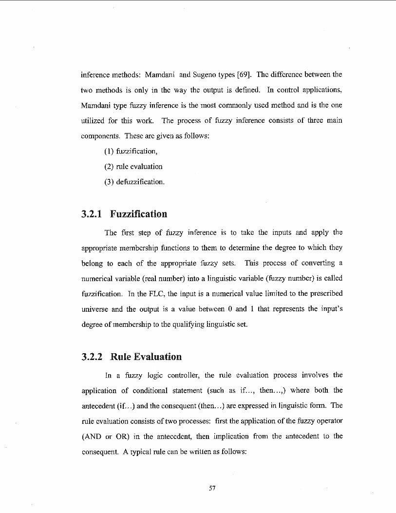
inference methods: Mamdani and Sugeno types [69]. The difference between the
two methods is only in the way the output is defined. In control applications,
Mamdani type fuzzy inference is the most commonly used method and is the one
utilized for this work. The process of fuzzy inference consists of three main
components. These are given as follows:
( 1) fuzzification,
(2) rule evaluation
(3) defuzzification.
3.2.1 Fuzzification
The first step of fuzzy inference is to take the inputs and apply the
appropriate membership functions to them to determine the degree to which they
belong to each of the appropriate fuzzy sets. This process of converting a
numerical variable (real number) into a linguistic variable (fuzzy number) is called
fuzzification. In the FLC, the input is a numerical value limited to the prescribed
universe and the output is a value between 0 and 1 that represents the input's
degree of membership to the qualifying linguistic set.
3.2.2 Rule Evaluation
In a fuzzy logic controller, the rule evaluation process involves the
application of conditional statement (such as if..., then ... ,) where both the
antecedent (if...) and the consequent (then ... ) are expressed in linguistic form. The
rule evaluation consists of two processes: first the application of the fuzzy operator
(AND or OR) in the antecedent, then implication from the antecedent to the
consequent. A typical rule can be written as follows:
57

Rule Ri: If L\co is A and L\e is B then Te is C.
where speed error L\co and change of speed error L\e are the input linguistic
variables, current I is the output linguistic variable and Ai, Bi, and Ci are the labels
oflinguistic variables L\co, L\e and I, respectively. lfthe antecedent is true to some
degree of membership then the consequent is also true to that same degree. The
fuzzy operators used for fuzzy rules are AND (n), OR (u) and NOT (- ). They
are defined as follows:
a) AND means classical intersection: mAna= min{mA(x), ms(x)}
b) OR means classical union: mAuB = max{mA(x), ms(x)}
c) NOT means classical complement: rnA = 1- mA(x).
Therefore, according to rule, the rule Ri, mci(x)=min{mAi(x), mBi(x)} .
3.2.3 Aggregation and Defuzzification
Defuzzification is the process of fuzzy inference that generates the final
output. But before the process of defuzzification can be completed, there is another
process, called the aggregation process, which must be evaluated.
The resultant decisions made by the FLC are based on the testing and
combining of all the rules in the fuzzy inference system. The process of combining
the fuzzy sets that represents the output of each rule into a single fuzzy set is called
the aggregation process.
The defuzzification process is the reverse of the fuzzification process. The
input for defuzzification is the combined output of each rule (the result of
aggregation process) and the output is a single number. Several different
defuzzification methods exist. In this work, the method was chosen by
compromising the accuracy of the outcome to reduce the computational burden
58

imposed in calculating it. The centre of gravity method was used, which IS
evaluated as,
N
Llimci(Ii) output I= ...:..i=-'-~----
Imci(Ii) i=l
(3 .5)
where N is the total number of rules, illci(Ii) denotes the output membership grade
for the ith rule with the output subset of Ii. An illustration of this process is shown
in Fig. 3.2.
Rule 1:
Rule 2:
1. Fuzzification of inputs
if Aro is PS (positive small)
if Aro is PM (*ositive medium)
Aro
Input 1
2. Application of fuzzy AND (min) operator
if Ae is NE (negative)
Ae
Input 2
3. Application of fuzzy implication method (min.)
then Te is NS (negative small)
then T e is PS (positive small)
Aggregation method (max.)
and Defuzzification (COG method)
Output 'Te'
Fig. 3.2. Overview of the complete fuzzy inference.
59

3.3 Fuzzy Logic Controller for IPMSM Drive
In the interior permanent magnet synchronous motor, the permanent
magnets are buried within the rotor core in order to produce a smooth rotor surface
and reduced air gap between the stator and the rotor. This allows the motor to be
used at high speeds with improved dynamic performance compared to other types
of permanent magnet motors. However, the operation of IPMSM is strongly
affected by rotor magnetic saliency, core saturation and armature reaction effects
due to the d-axis stator current id. The saturation of the rotor iron around the
permanent magnets produces significant distortion of the air gap flux and causes
the reactance parameters to vary with different operating conditions. These
nonlinearities affect the performance of the drive at different dynamic operating
conditions.
These factors can be overcome by use of artificial intelligence based
controllers, capable of handling any nonlinear functions of arbitrary complexity. A
fuzzy logic controller has been proposed for the IPMSM drive. The use of a fuzzy
logic controller (FLC) for the IPMSM drive in high performance applications bas
the following benefits:
(a) The system mathematical model is not required: The FLC does not need
any information of the exact system mathematical model. This makes it one of
the best approaches for control of an IPMSM motor drive, where the exact
system mathematical model is difficult to obtain and includes dynamically
changing parameters.
(b) The FLC is self-adaptive: In the real-time IPMSM drive reactance
parameters change with operating conditions, resistance changes with
60

temperature, inertia changes with mechanical load variation and command
speed may be changed on demand. The FLC self-adapts to these changing
conditions and hence can be used as a robust controller for the IPMSM drive.
(c) Reasonable cost: The application of other types of intelligent controllers
to the IPMSM drive for high performance applications requires sophisticated,
and often expensive, hardware. While the use of the FLC also requires a degree
of specialized hardware, it is less complex than other intelligent controllers and
therefore is considered cost effective.
3.3.1 FLC Structure for the IPMSM Drive
The motor dynamics can be represented by the following equation:
Te = TL + BmCOr + lmPCOr (3.6)
where T e is the electrical torque, T L is the load torque, Bm is the friction damping
coefficient, Jm is the rotor inertia constant, p is the differential operator and COr is
rotor speed.
The dynamic model of the IPMSM can be rewritten from Eqns. (2.21) and
(3.6) as,
(3.7)
61
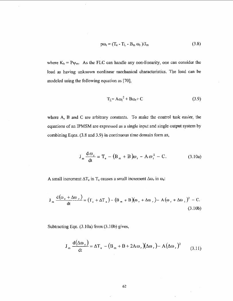
(3.8)
where Kb = P'l'm· As the FLC can handle any non-linearity, one can consider the
load as having unknown nonlinear mechanical characteristics. The load can be
modeled using the following equation as [70],
(3.9)
where A, B and C are arbitrary constants. To make the control task easier, the
equations of an IPMSM are expressed as a single input and single output system by
combining Eqns. (3.8 and 3.9) in continuous time domain form as,
(3.10a)
A small increment ATe in T e causes a small increment Aror in ror:
Subtracting Eqn. (3.10a) from (3.10b) gives,
d(11roJ ( X ) ( )2 J m = 11 T e - B m + B + 2A ffi r 11m r - A 11m r dt (3.11)
62

By replacing all the continuous quantities of Eqn. (3.11) by their finite
differences, the discrete time small signal model of the simplified IPMSM with
nonlinear load can be given as,
Hence,
Te(n) = f~T e(n) = f(~e(n), ~wr(n), wr(n)) (3.13) discrete
where, 1\e(n) = ~ror(n) - 1\ror(n-1) is the change of speed error, 1\ror(n) = ro/ (n) -
ror(n) is the present sample of speed error, ~ror(n-1) is the past sample of speed
error, ror(n) is the present sample of actual speed, ror"(n) is the present sample of
command speed, ts is the sampling time interval and f denotes the nonlinear
function. Thus, the purpose of using the FLC is to map the nonlinear functional
relationship between electrical torque T e and rotor speed ror.
From this command torque Te, Eqns. (2.36) and (2.37) are used to calculate
the necessary q- and d-axis currents to produce the rotor speed ror. In real-time, the
motor position information and the output of the simplified FLC in terms of the
command q-axis and d-axis currents iq * and id * are used to get the motor command
phase currents ia*, ib* and i/ by using Park's transformation.
63

3.3.2 Simplified FLC for the IPMSM Drive
The model of the IPMSM expressed by Eqn. (3.13) defines the input and
output linguistic variables for the FLC of the IPMSM drive. According to Eqn.
(3.13), the inputs of the proposed FLC are the present samples of speed error,
change of speed error (which is the difference between the present and past samples
of speed error) and present rotor speed. However, it has been observed that the
effect of the inclusions of the rotor speed and change of speed error on motor speed
response is negligible, not producing an improvement in drive performance
commensurate with the resulting increase in computational burden as compared to
the case when it is omitted. The omission of the cor(n) and ~e(n) terms produces a
proportional-type FLC-based drive with acceptably responsive and accurate
tracking of the command speed. Thus, the input vectors of the FLC can be reduced
to only ~cor(n), producing a much-simplified FLC as compared to input vectors of
~cor(n), ~e(n) and cor(n) with the non-simplified system. These simplifications
significantly reduce computational burden and lower the computer memory and
power required to implement the FLC scheme in real time. Thus, this simplified
FLC is a significant factor for real-time implementation of the laboratory IPMSM
drive system, if a fuzzy-based controller is to be employed. The block diagram of
the proposed FLC based IPMSM drive incorporating MTPA is shown in Fig. 3.3.
Next, scaling factors, Koo and Ki, are chosen for fuzzification and obtaining
the appropriate actual output of the command current. The factor Kco is chosen so
that the normalized value of speed error, ~com, remains within the limits of± 1.
The factor Ki is chosen so that rated current is produced by the controller at rated
conditions. The constants are taken as Koo = co/ (command speed) and Ki = 10 in
order to get the optimum drive performance.
64

Simplill.ed FLC
-00 (.k) d dt
Hall-effect Sensors
AID Col'W'el'te:r
Fig. 3.3. Block diagram of proposed simplified FLC
-based IPMSM drive with MTP A control.
After selecting the scaling factors, the next step is to choose the
membership functions of ~rom and the normalized command torque Ten*, which
form an important element of the FLC.
The membership functions used for the input and output fuzzy sets are
shown in Fig. 3.4. Trapezoidal functions are used as membership functions for all
the fuzzy sets with the exception of the fuzzy set ZE (zero) of the input vector.
Triangular membership functions are used for the fuzzy set ZE of the input vector
and all the fuzzy sets of the output vector. The trapezoidal and the triangular
functions are used because of their mathematical simplicity, and thus to simplify
65

implementation and reduce computational burden for real-time implementation.
The non-symmetrical nature of the membership functions were arrived at by trial
and error.
1 FNH ___ ---,--___,..._....~ .. · · .;;,·"·~.·-~--P-L...---..,......
0_5 r (a)
PH ·-i
0.6 0.8
0.4 0.6 0. 8
Fig. 3.4. Membership functions for: (a) normalized speed error ~ffirn,
(b) normalized command torque Ten*.
66

The rules used for the proposed FLC algorithm are as follows:
i) if Llrom is PH (positive high), Ten is PH (positive high).
ii) if Llrom is PL (positive low), Ten is PM (positive medium).
iii) if Llrorn is NL (negative low), Ten is NL (negative low).
iv) if Llrom is NH (negative high), Ten is NH (negative high).
v) if Llrorn is ZE (zero), Ten is NC (no change).
In this work, the values of the constants, membership functions, fuzzy sets
for the input/output variable and the rules used were selected by trial and error in
order to obtain the optimum drive performance.
3.4 Concluding Remarks
The principles of the fuzzy logic controller for IPMSM control applications
have been presented in this chapter. A specific simplified fuzzy logic controller is
proposed for the IPMSM motor drive as a robust speed controller in order to
overcome the problems caused by real-time motor parameter variations, load
changes and system disturbances.
67

Chapter 4
Simulation of the FLC Based Vector
Control of the IPMSM
4.1 General Introduction
This chapter presents a neoteric speed control technique for the IPMSM
based around both fuzzy logic and the maximum torque per ampere (MTPA), with
Taylor series approximation, mode of operation. For comparison purposes, two
separate fuzzy logic based speed controllers have been implemented. The first is a
FLC based controller operating under the id = 0 assumption, based on previous
work by M. N. Uddin [63]. The second is a new, simplified FLC/MTPA based
system designed around the mathematical model of the IPMSM, the appropriate
motor dynamics and the nonlinear load model. This design has been developed in
chapter 3, is illustrated in Fig. 3.4 and simulation model details are presented in
Appendix B.
Extensive simulations have been done in order to predict the performances
of the drives using the two FLC based systems at different dynamic operating
conditions.
Finally the simulation results have been presented and discussed.
68
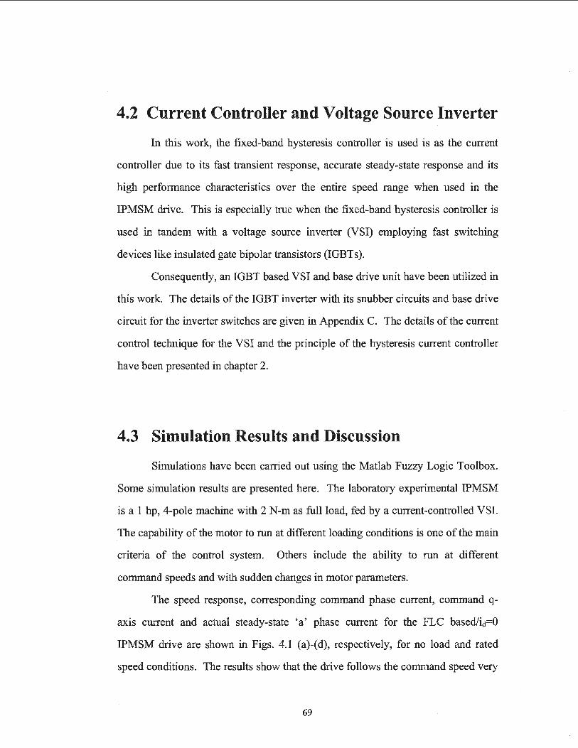
4.2 Current Controller and Voltage Source Inverter
In this work, the fixed-band hysteresis controller is used is as the current
controller due to its fast transient response, accurate steady-state response and its
high performance characteristics over the entire speed range when used in the
IPMSM drive. This is especially true when the fixed-band hysteresis controller is
used in tandem with a voltage source inverter (VSI) employing fast switching
devices like insulated gate bipolar transistors (IGBTs).
Consequently, an IGBT based VSI and base drive unit have been utilized in
this work. The details of the IGBT inverter with its snubber circuits and base drive
circuit for the inverter switches are given in Appendix C. The details of the current
control technique for the VSI and the principle of the hysteresis current controller
have been presented in chapter 2.
4.3 Simulation Results and Discussion
Simulations have been carried out using the Matlab Fuzzy Logic Toolbox.
Some simulation results are presented here. The laboratory experimental IPMSM
is a 1 hp, 4-pole machine with 2 N-m as full load, fed by a current-controlled VSI.
The capability of the motor to run at different loading conditions is one of the main
criteria of the control system. Others include the ability to run at different
command speeds and with sudden changes in motor parameters.
The speed response, corresponding command phase current, command q:.
axis current and actual steady-state 'a' phase current for the FLC basedlid=O
IPMSM drive are shown in Figs. 4.1 (a)-(d), respectively, for no load and rated
speed conditions. The results show that the drive follows the command speed very
69

quickly without any overshoot and nearly zero steady-state error. The command q
axis current, which also represents the command torque (since id has been forced to
zero in this scheme), however, oscillates significantly at steady-state conditions.
This does not appear to significantly impact operational performance.
Figs. 4.2 (a)-(d) show the speed response, command phase current ia*, q-axis
command current and steady-state phase current ia, respectively, for the FLC
basedlid=O IPMSM at half load and rated speed conditions. Again the drive follows
the command speed without any overshoot or steady-state error, but the command
q-axis current, and hence the command torque, oscillates greatly at steady-state,
although the actual phase current is almost sinusoidal.
The similar responses of the FLC basedlid = 0 IPMSM drive at full load and
rated speed conditions are shown in Figs. 4.3 (a)-(d). Under these conditions,
phase current magnitude peaks at 3.3 amperes, which is 10% in excess of the rated
current of 3 amperes. This is due to the fact that the id = 0 approximation induces a
higher stator command current than ideally with id not forced to zero. Once again,
it is shown that the drive can follow the command speed smoothly without any
overshoot and steady state error. These results verify that the FLC/ id=O based
IPMSM drive can follow the command rated speed at various loading conditions.
A step change of command speed is applied to the FLC basedlict=O drive in
order to evaluate drive performance in terms of response time, speed overshoot,
transient and steady state errors and stability. This is necessary because in high
performance drive applications it is essential to change command speeds with
situational demands. The responses of the drive including speed, ' a' phase
command current, q-axis command current and steady-state actual phase current
are shown in Figs. 4.4 (a)-(d), respectively, for a step change of command speed at
70

half load conditions. The results show that the drive can follow the command
speed without overshoot and steady-state error during a step increase of speed (1 00
rad./sec.~ 188.5 rad./sec.) but there is a small, but acceptable, undershoot during a
step decrease of speed (188.5rad./sec.~100rad./sec.). Again, q-axis command
current, and hence command torque, oscillates significantly, though this does not
appear to significantly impact drive performance. The results show that the FLC
basedlid=O drive can follow the command speed even after a step change of
command speed.
The ability of the drive to withstand disturbances is another important
feature of the control system. Change of load is a typical external disturbance and
is a very common occurrence for a high performance drive. The speed and
corresponding command a-phase current ofthe motor, q-axis command current and
steady-state actual a-phase current responses for the FLC based/id=O drive are
shown in Figs. 4.5 (a)-( d), respectively, for a sudden increase of load at the rated
speed. The motor is started with half load and at t = 0.25 sec. the load is suddenly
increased to full load. It is shown that drive speed is reduced transiently, and only
modestly, and that command speed is quickly recovered even under this relatively
dramatic increase of load. The current response is almost sinusoidal and follows
command current. Command torque, as indicated by iq"' oscillates greatly, but this
does not appear to negatively effect drive performance.
The speed response, corresponding command phase current, command q
axis current and actual steady-state 'a' phase current for the simplified FLC
based!MTPA IPMSM drive are shown in Figs. 4.6 (a)-( d), respectively, for no load
and rated speed conditions. The results show that the drive follows the command
71
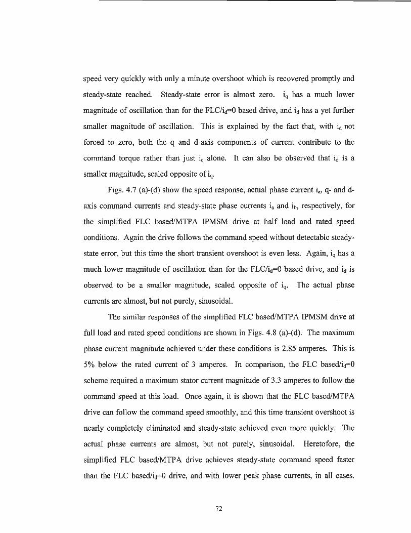
speed very quickly with only a minute overshoot which is recovered promptly and
steady-state reached. Steady-state error is almost zero. iq has a much lower
magnitude of oscillation than for the FLC/id=O based drive, and id has a yet further
smaller magnitude of oscillation. This is explained by the fact that, with id not
forced to zero, both the q and d-axis components of current contribute to the
command torque rather than just iq alone. It can also be observed that id is a
smaller magnitude, scaled opposite of iq.
Figs. 4.7 (a)-( d) show the speed response, actual phase current ia, q- and d
axis command currents and steady-state phase currents ia and ib, respectively, for
the simplified FLC based/MTP A IPMSM drive at half load and rated speed
conditions. Again the drive follows the command speed without detectable steady
state error, but this time the short transient overshoot is even less. Again, iq has a
much lower magnitude of oscillation than for the FLC/id=O based drive, and id is
observed to be a smaller magnitude, scaled opposite of iq. The actual phase
currents are almost, but not purely, sinusoidal.
The similar responses of the simplified FLC based/MTP A IPMSM drive at
full load and rated speed conditions are shown in Figs. 4.8 (a)-( d). The maximum
phase current magnitude achieved under these conditions is 2.85 amperes. This is
5% below the rated current of 3 amperes. In comparison, the FLC basedlid=O
scheme required a maximum stator current magnitude of 3.3 amperes to follow the
command speed at this load. Once again, it is shown that the FLC based/MTP A
drive can follow the command speed smoothly, and this time transient overshoot is
nearly completely eliminated and steady-state achieved even more quickly. The
actual phase currents are almost, but not purely, sinusoidal. Heretofore, the
simplified FLC based/MTP A drive achieves steady-state command speed faster
than the FLC based/id=O drive, and with lower peak phase currents, in all cases.
72

These results verify that the FLC based/MTP A IPMSM drive can quickly achieve
and follow the command rated speed under various loading conditions.
Figs. 4.9 (a)-(d) show the speed response, actual phase current ia, q- and d
axis command currents and steady-state phase currents ia, ib and ic, respectively, for
the simplified FLC based/MTP A IPMSM drive at full load + 25% and rated speed
conditions. Command speed is achieved very quickly, with practically no
overshoot or oscillation. Maximum phase current magnitude under these
conditions is 3.3 amperes, the same magnitude required by the FLC based/id=O
drive to achieve rated speed at full load conditions.
Figs. 4.10 (a)-( d) show the speed response, actual phase current ia, q- and d
axis command currents and steady-state phase currents ia, ib and ic, respectively, for
the simplified FLC based/MTP A IPMSM drive at full load and low speed
conditions (75 rad./sec.). There is some oscillation in reaching command speed but
this is quickly damped and steady-state reached in under 0.05 sec. The actual phase
currents exhibit almost, but not purely, sinusoidal behavior with peak values well
below rated current.
The responses of the FLC based!MTP A drive including speed, 'a' phase
actual current, q- and d-axis command currents and steady-state actual phase
currents to a step change of command speed at half load are shown in Figs. 4.11
(a)-(d), respectively. The results show that the drive can follow the command
speed quickly and accurately during a step increase (100 rad./sec.~1 88.5 rad./sec.)
and decrease (188.5rad./sec.~100rad./sec.) of speed, but there are small, but
acceptable, overshoots and undershoots which are recovered promptly.
Figs. 4.12 (a)-( d) show the speed response, actual phase current ia, q- and d
axis command currents and command phase current imposed over actual phase
current, respectively, for the simplified FLC based/MTPA IPMSM drive to a step
73

change of command speed at full load conditions. Once again, it is shown that the
drive quickly and accurately follows command speed. It can also be observed that
actual phase current follows command current. The results show that the FLC
based!MTP A drive can follow the command speed even after a step change of
command speed at different loading conditions.
The ability of the drive to withstand disturbances is another important
feature of the control system. Change of load is a typical external disturbance and
is a very common occurrence for a high performance drive. The speed and
corresponding actual a-phase current of the motor, q- and d-axis command currents
and steady-state actual a-phase current responses for the FLC based/MTPA drive
are shown in Figs. 4.13 (a)-( d), respectively, for a sudden increase of load at rated
speed. The motor is started with half load and at t = 0.25 sec. the load is suddenly
increased to full load. It is observed that drive speed is reduced transiently, and
only very slightly, and that command speed is recovered extremely quickly, even
under this relatively dramatic increase of load. The current response is almost
sinusoidal and follows command current.
Because IPMSM parameters are affected significantly by saturation and
temperature, one of the most important criteria of the control system for the
IPMSM drive is the ability to withstand motor parameter variations. The change of
stator resistance with temperature is a common phenomenon in such machines.
The speed and corresponding actual phase current responses of the FLC
based/MTPA drive are shown in Figs. 4.14 (a) and (b), respectively, for doubled
stator resistance at no load and rated speed conditions. The similar responses for
full load conditions are shown in Figs. 4.15 (a) and (b). In both cases it is shown
74

that the drive follows the command speed even after a sudden and dramatic change
of armature resistance.
Additionally, the inertia of the motor may change at different loading
conditions, so it is important to investigate the response of the drive to inertia
variations. Figs. 4.16 (a) and (b) show the speed and corresponding actual 'a'
phase current responses, respectively, to a sudden doubling of rotor inertia under no
load conditions at rated speed. Figs. 4.17 (a) and (b) show the similar responses
under full load conditions. These results indicate that the FLC based/MTP A drive
follows the rated command speed accurately and smoothly even when subjected to
a sudden doubling of rotor inertia under different loading conditions.
In the IPMSM changes in d- and q-axis reactance parameters during
operation can significantly affect drive performance. This can be easily understood
as the torque equation (2.29) contains both the d- and q-axis inductance parameters.
Therefore, high performance drives must be able to respond quickly and accurately
to variations in Lq and Ld. Figs. 4.18 (a) and (b) show the speed and corresponding
actual ' a' phase current responses, respectively, to a sudden 50% decrease in Lq
under no load at rated speed. Figs. 4.19 (a) and (b) show the similar responses
under full load conditions. These results indicate that the FLC based/MTP A drive
follows the rated command speed accurately and smoothly even when subjected to
a sudden 50% decrease of Lq under different loading conditions.
75

200~-~---,---~--~-~
. 150 ···-····-····· .. ··'· <.J (I)
~ '0 ~100 .
-r:i (I) (I) Cl. (/) 50
0.2
10
<(
• .Q'
0 .4 0.6 Time, sec.
(a)
) ......... .
0.8
10
(d) 6
<(
.~ 2
-2
-60 0.2 0.4 0 .6 0.8 Time, sec.
Fig. 4.1. Simulated responses of the FLC basedlid=O IPMSM drive: a) speed, (b)
command phase current, (c) q-axis command current and (d) steady-state actual
phase current at no load and rated speed conditions.
76

0150 Q)
~ "'0 ~100 -ci Q) Q) c.. en so
%L_--~0~.2--~0~.4~--0~.6----j0.8~~
Time, sec.
<(
0.2 0 .4 0.6 Time, sec.
0.8
-BOL__ ___ OL.2----:0~.4----0c'-.6----0-L.8--____j
Time, sec.
Fig. 4.2. Simulated responses of the FLC based/id=O IPMSM drive: a) speed, (b)
command phase current, (c) q-axis command current and (d) steady-state actual
phase current at half load and rated speed conditions.
77

200,--~--.,....----,---~----,
··-~ ·· u1so I -· Q)
~ "0 l!! 100
-g Q) c.. (/) 50
%~-~0~.2-~0~.4~-0~.6~-~-~
Time, sec.
(cy ·-·
<t.: <t.: .!!i
0.4 0.6 Time, sec.
0.8
Fig. 4.3. Simulated responses of the FLC based/id=O IPMSM drive: a) speed, (b)
command phase current, (c) q-axis command current and (d) steady-state actual
phase current at full load and rated speed conditions.
78

-10oL----=o-'-=-.2----:0:c'-c.4,--·- a"".6,----=-'o.s:---
Time, sec.
Fig_ 4.4. Simulated responses of the FLC based/id=O IPMSM drive: a) speed, (b)
command phase current, (c) q-axis command current and (d) steady-state actual
phase current for a step change of speed at half load conditions.
79
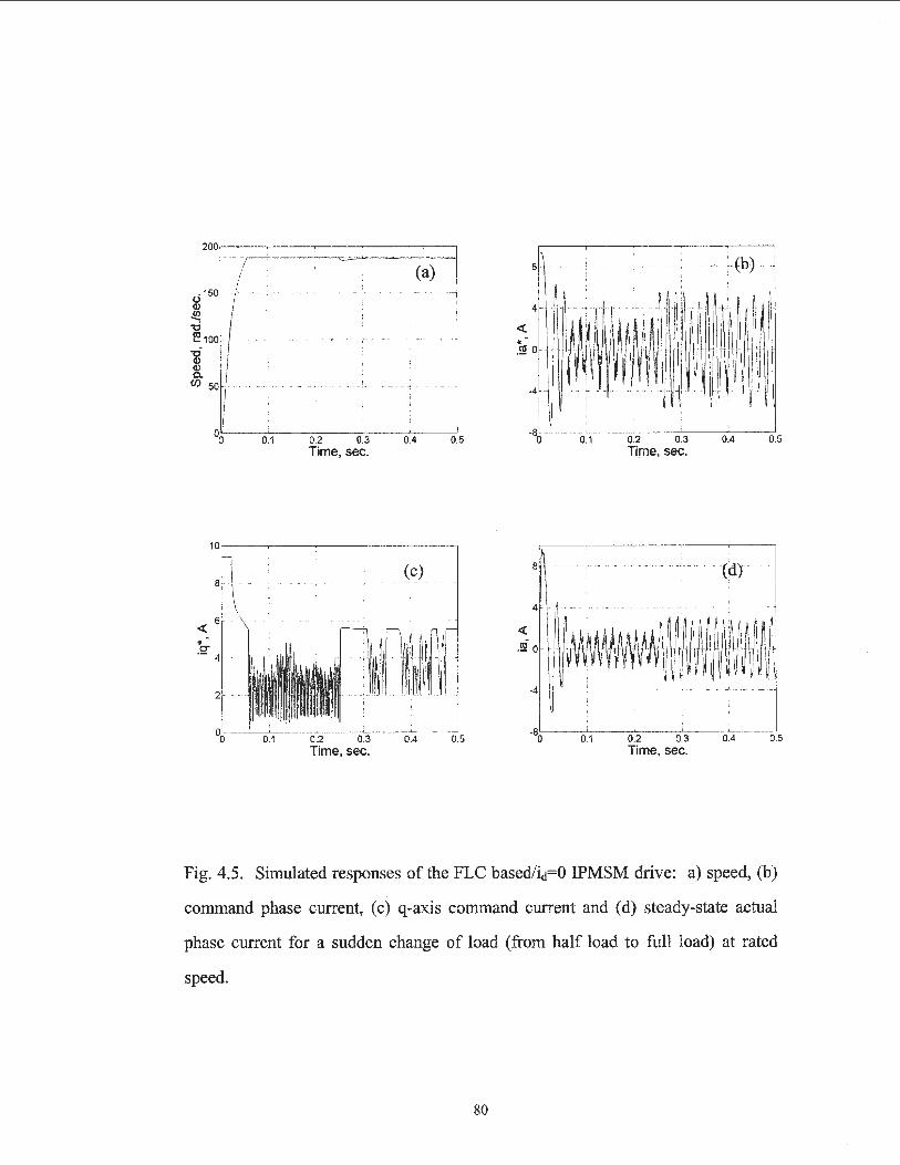
200,--~--~--.---~---,
. 150 ..... ······ ' .. .. . (,) <11.
..!!! -c ~ 100 ... .. . .. .. . ' .. ... . .
"C <11 <11 c.
Cl) 50~·~· ~ . .. .... L_j__J
0o 0.1 0.2 0.3 0.4 0.5
Time, sec.
<(
• . 2'
8 i{b)
4
<(
• . !!1 0
-4 ...
"8o[__~0.-1 -~0.2--0,-L.3----::0.L.4_--,J0.5 Time, sec.
-so[_ _ __io.-1 --o~.2- o.3 0.4 0.5 Time, sec.
Fig. 4.5. Simulated responses of the FLC based/id=O IPMSM drive: a) speed, (b)
command phase current, (c) q-axis command current and (d) steady-state actual
phase current for a sudden change of load (from half load to full load) at rated
speed.
80

200~-~----,---~-~--
.150 .. 0 Q.l
~ "0 f! 100
-c Q.l Q.l c.
(f) 50 .. .... . -- . .
0.2
0.2
0.4 0.6
0.4 0.6 Time, sec.
, (a)
0.8
0.8
<(
0.2
4 - ...
-4
··· ········-- --.. -- -- -·· ·
0.4 0:6 Time, sec.
(b)
0.8
(d)
! •.. ~ \ .... . -. ..... --
-8o!-----="o.-=-2 ---=-"o.4-=----o=-'=_6,----:o~.8-Time, sec.
Fig. 4.6. Simulated responses of the simplified FLC based/MTP A IPMSM drive:
a) speed, (b) command phase current, (c) q-axis and d-axis command currents and
(d) steady-state actual phase current at no load and rated speed conditions.
81

200,----,--~--,.----,------,
-(a) .150 ...
al ~
··- ···· ·······-- ..... --- ...... •.. t
"0 I!! 100 ...
a1-<ll 0. en so ... -- ... -- ~ .. ...... . ........ . '!
~~-~0.72-~0.4~-0~.6-~0~.8-~ Time, sec.
"12o:-- -:co'=".2 -----::co'-:".4 ---::"o_-=-6 --='o.-=-e --1
Time, sec.
<(
(b) 4 .. . ' . ................. .
"8ol.___~o . ..,...2 -~0.4--0-'-.6----::-'-c---~
Time, sec.
3
-3 ... ............. , .. - . ... ... .
·8.'=-2 --0~.2=2 ---=o=-'=.2-:-4 --=o-':c.26
Time, sec.
(d)
0.28 0.3
Fig. 4.7. Simulated responses of the simplified FLC based/MTPA IPMSM drive:
a) speed, (b) steady-state actual phase current, (c) q-axis and d-axis command
currents and (d) steady-state actual phase currents ia and ib at half load and rated
speed conditions.
82

200~-~-~--~-~-~
0.4 0.6 Time, sec.
Tim<> C:<>f'
. (a)
0.8
<(
.~
<(
S r. -~--~-~--~-~
2.5 .
0.31 0.32 0.33 Time, sec.
0.34 0.35
Fig. 4.8. Simulated responses of the simplified FLC based!MTPA IPMSM drive:
a) speed, (b) steady-state actual phase current, (c) q-axis and d-axis command
currents and (d) steady-state actual phase currents ia, ib and ic at full load and rated
speed conditions.
83

200,---~-~,..---------,--~---,
. 150 (.) Q)
~ "0 ~100 -g
~-----~-------~-~ ;
(a)
. .. ~. ... ..
4
~ 0 ·· .!2
(b) ' ' \, ........ -~-· ··•·· .. :.. ... .
Q) a. en so
0.2 0.4 0.6 Time, sec.
· · ~~~~·*~ :OL.:_-~---:'·":--··_··-·_·· ·--:-r . r n ·· ~
0.2 0.3 0.4 0.5
' \ • . . . . .. (c) '
~:~ ~ ~~~~,~~,'V~ ,g :.=... -4 .. ...... . -· ... ...... ~- · . . ~
-8
-12o--o,..L: 1---="o.2=-----=o"=-.3----::"-o.4.,-------,J0.5
Time, sec.
Tim~ c:~r
0.31 0.32 0.33 0.34 0.35 Time, sec.
Fig. 4.9. Simulated responses of the simplified FLC based/MTPA IPMSM drive:
a) speed, (b) steady-state actual phase current, (c) q-axis and d-axis command
currents and (d) steady-state actual phase currents ia, ib and ic at full load + 25% and
rated speed conditions.
84

80 8
(a) (b)
. 60 4 \ ... ..... · ·· ·~· . ,_ .........
u Q) Vl .._ -o <( ~40 .!§ 0 -o Q) Q) c.
(/)20 -4
0o---o:2 0.4 0.6 0.8 -80 0.2 0.4 0.6 0.8
Tim~'> .. ,.,. Time, sec.
"12oe...._ __ 0~.2--0~.4--0-'-.6---~0.8 __ _
Time, sec.
Fig. 4.10. Simulated responses of the simplified FLC based!MTPA IPMSM drive:
a) speed, (b) steady-state actual phase current, (c) q-axis and d-axis command
currents and (d) steady-state actual phase currents ia, ib and ic at full load and low
speed (75 rad./sec.) conditions.
85

160
0 m. VI :;; 120 .
e! -g 80 (1) c. (/)
;
l·
40 ........... ..... , ..
%-L_--~0~.2----0~.4~--0~.6----~0.8--~
Time, sec.
0.2 0.4 0.6 Time, sec.
0.8
<(
.!2
' 10oL_ ___ 0~.2----0~.4----0::"c.6,-l-__ .,.._0.8
Time, sec.
Fig. 4.11 . Simulated responses of the simplified FLC based!MTPA IPMSM drive:
a) speed, (b) steady-state actual phase current, (c) q-axis and d-axis command
currents and (d) steady-state actual phase currents ia, ib and ic for a step change of
speed at half load conditions.
86

200,.----~---.---,---------,------,
~150
.!!! -c f! 100fl;---_;_---'
i a. (f) 50 ·····
, (a)
%~-~0~.2~-~0.4~-~0~.6-~0~.8-~ Time, sec.
"15o:---'""'o:-':.2~--=-'o.4-=----:co7.6-----=o"'=. 8~_..
Time, sec.
·10o':---~o"=.2---=-'o.4~-~o7.6 ..L-----=o"'=.8-. ___ J
0.76
Time, sec.
0.77 0.78 Time, sec.
0.79 0.8
Fig. 4.12. Simulated responses of the simplified FLC based/MTPA IPMSM drive:
a) speed, (b) steady-state actual phase current, (c) q-axis and d-axis command
currents and (d) steady-state actual and command phase currents ia and ia* for a step
change of speed at full load conditions.
87
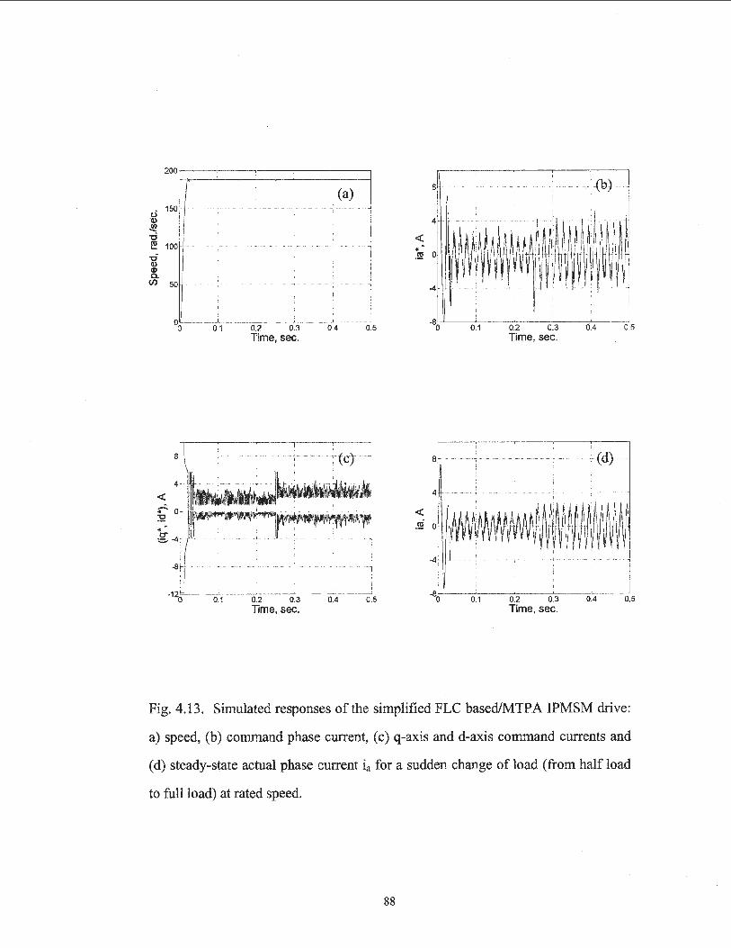
200 ·---~
u 150 (I)
~ "C co .... 100
-c (I) (I) c.
C/) 50
00
....... -T . .......... ... ...... .............. ...... ~ ..
·--· .. ·-
;
--~
0.1
0.1
0.2 0.3 Time, sec.
0.2 0.3 Time, sec.
i (a)
0.4
0.4
I <( .
0.5
0.5
....... . --- ---- --·-··"·····--···· ..... : (b) ----
;
---
.~~~ · ~ {fM~~~ -4 .. . - - -
-80 0.1 0.2 0 .3 0.4 0.5 Time, sec.
'
-~~ ·Bo:-· --='o_-:-1 -----::":o.2=-----co::':_3c----:o:>-:-.4---::-o_s
Time, sec.
Fig. 4.13. Simulated responses of the simplified FLC based/MTPA IPMSM drive:
a) speed, (b) command phase current, (c) q-axis and d-axis command currents and
(d) steady-state actual phase current ia for a sudden change of load (from half load
to full load) at rated speed.
88

200,...---~-~---,---~-~
. 150 u Q)
~ "C !!! 100 "C Q) Q) Q.
en so
<( - 0
.!!1
-4
-• • · - M ' · •· · · • . .
0.1 0.2 0.3 Time, sec.
.Ja)_
0.4 0.5
(b)
Fig. 4.14. Simulated responses of the simplified FLC based/MTPA IPMSM drive:
a) speed, (b) steady -state actual phase current ia for a sudden change of stator
resistance (R to 2R) at no load and rated speed.
89

200,----~-~--.-----r-----;
e,j 150 Q)
~ -o e! 100 -'0
~ (/) 50
--~----.----~--~---~
.... {~) ..... .
0.1 0.2 0.3 0.4 0.5
a~-~:--~-~--~-~
(~) 4 ... ·• · .. ( . ·····
-4 .... ........ .. ... ··- ... .. . ... • . ... ........ .
-80 0.1 0.2 0:3 Time, sec.
0.4 0.5
Fig. 4.15. Simulated responses ofthe simplified FLC based!MTPA IPMSM drive:
a) speed, (b) steady-state actual phase current ia for a sudden change of stator
resistance (R to 2R) at full load and rated speed.
90

-80 0.1 0.2 0 .3 Time, sec.
.. (~) .. ...
(b)
' .... ·-~ ..... ;
0.4 0.5
Fig. 4.16. Simulated responses of the simplified FLC based/MTP A IPMSM drive:
a) speed, (b) steady-state actual phase current ia for a sudden change of rotor inertia
(J to 2J) at no load and rated speed.
91

200
0 Q) VI ~120 " '"t
!!! 't:l 80 Q) Q) 0. U')
.. . ;.
00 0.1
4
-80 0.1
:
0.2 0.3 Time, sec.
0.2 0.3 Time, sec.
... ,
(a)
0.4 0.5
(b)
0.4 0.5
Fig. 4.17. Simulated responses of the simplified FLC based!MTP A IPMSM drive:
a) speed, (b) steady-state actual phase current ia for a sudden change of rotor inertia
(J to 2J) at full load and rated speed.
92

200~-~--~-~--~-~
g150
~ -c::i ~100
"C Q) Q) 0.
(1,) 50
0.1
. ., .. , ~ .... .. _.......... . .. . . ""i'
0.2 0.3 Time, sec.
0.4 0.5
s~-~--~-~--~--.
-80 0.2 0.3 Time, sec.
0.5
Fig. 4.18. Simulated responses of the simplified FLC based/MTPA IPMSM drive:
a) speed, (b) steady-state actual phase current ia for a sudden 50% decrease ofLq at
no load and rated speed.
93

%~--~o_~,---o~.2~~o~.3--~0~.4--~0.5
T im&:tt c:~,..
a~--~--~----~--~--~
:
4
<( -0
.!11
(b) ...
: l • • • ' . ' '
, : . I ' \ ; :
~~MWr · ·. · fM -4 I ····· .... ' '· ·· .... , __ · ·-- ... ..
-80 0.1 0.2 0.3 0.4 0.5
Tim<> "'""
Fig. 4.19. Simulated responses of the simplified FLC based/MTPA IPMSM drive:
a) speed, (b) steady-state actual phase current ia for a sudden 50% decrease of Lq at
full load and rated speed.
94

4.4 Concluding Remarks
The simulation results show encouraging performances of the proposed
drive. The simplified FLC can accommodate different operating conditions such as
load change, parameter variations and step change of command speed. Therefore,
the simplified FLC with MTPA can be a good substitute for the conventional fixed
gain PI or PID controllers or for more complex FLC schemes.
Generally, as the number of fuzzy rules increase better performance can be
attained, but by use of the maximum torque per ampere with Taylor series
approximation scheme, and the prudent simplification of the fuzzy algorithm, high
performance can be obtained along with a reduction of computational burden. The
simulation results confirm the robustness of the simplified FLC/MTP A controller
in an IPMSM drive.
In order to validate the efficacy of the proposed drive, the laboratory
implementation of the complete vector control scheme of the drive has been carried
out in real-time as an integrated part of the proposed work. In addition, the non
simplified FLC with id = 0 drive has been implemented in the lab also.
95
Chapter 'S
Experimental Implementation of the
Simplified FLC Based MTP A Vector
Control of the IPMSM
5.1 General Introduction
The implementation of a fuzzy controlled drive often presents difficulties in
that the high computational burden imposed necessitates both high-level hardware
and software. Because of this, the real-time implementation of the FLC for motor
drives has presented a challenge to control engineers. This work overcomes such
problems by utilizing a simplified FLC along with an approximated MTP A
scheme.
The experimental implementation of the complete simplified FLC/MTP A
IPMSM drive is presented in this chapter. This is the first time that the maximum
torque per ampere mode of operation has been implemented with a fuzzy logic
controller for the IPMSM in real-time.
96

The drive has been realized by use of a PC interfaced with a current
controlled voltage source inverter through a dSP ACE DS 1102 digital-signal-
processor (DSP) controller board. This chapter presents the detailed
implementation of both hardware and software programming. In order to validate
the efficacy of the drive, various experimental results under different dynamic
operating conditions are presented and discussed.
5.2 Experimental Setup
5.2.1 Hardware Implementation
The hardware schematic for real-time implementation of the proposed
IPMSM drive is shown in Fig. 5.1. The DSP board was installed in a personal
computer (PC) with uninterrupted communication capabilities through dual-port
memory. The DS 1102 board is based on a Texas Instrument (TI) TMS320C31 32-
bit floating point digital signal processor. The DSP has been supplemented by a set
of on-board peripherals used in digital control systems, such as analog to digital
(A/D), digital to analog (D/A) converters and incremental encoder interfaces. The
DS1102 board has one 4 channel (2 12-bit and 2 16-bit) AID and one 4 channel
(12-bit each) D/A converter and two 16-bit incremental encoders. The DS1102 is
also equipped with a TI-TMS320Pl4 16 bit micro controller DSP that acts as a
slave processor and provides the necessary digital input/output (I/0) ports and
powerful timer functions such as input capture, output capture and PWM waveform
generation.
In this work, the slave processor was used only for digital I/0 configuration.
The actual motor currents were measured by Hall effect sensors, which have good
frequency response, and were fed to the DSP board through the AID converter. As
the motor neutral was not grounded, only two phase currents were fed back and the
97

other phase current calculated from them. The rotor position angle was measured
by an absolute incremental encoder mounted on the rotor shaft via a flexible
coupler, and fed to the DSP board through an encoder interface. The encoder
generates 4096 pulses per revolution, which are fed to the incremental encoder
interface of the board. By using a 4-fold pulse multiplication the output of the
encoder is increased to 4x4096 pulses per revolution in order to get a better
resolution. A 24-bit position counter is used to count the encoder pulses. The
counter is reset once per revolution by the index pulse generated from the encoder.
The motor speed was computed from the measured rotor position angles using
numerical differentiation.
In order to implement the vector control algorithm, the fixed-band
hysteresis controller was used as the current controller. The command currents are
generated from the speed controller. The hysteresis current controller compares the
command currents with the corresponding actual motor currents and generates the
logic signals, which act as firing pulses for the inverter switches. Thus, these six
PWM logic signals are the output of the DSP board and were fed to a base drive
circuit for the insulated gate bipolar transistor (IGBT) or bipolar junction transistor
(JCT) inverter power module. The base drive circuit was used to provide isolation
between the high power supply and the low power logic circuits and also to
improve the voltage level so that it is sufficient to drive the inverter. The de power
supply for the inverter was obtained by rectifying the ac power through a variac.
In order to provide loading, the laboratory IPMSM was coupled to a
dynamometer using a belt. The dynamometer serves as a simple mechanical load
on the motor. A digital storage oscilloscope was used to capture the desired signals
coming out through the D/ A port of the DSP board.
98
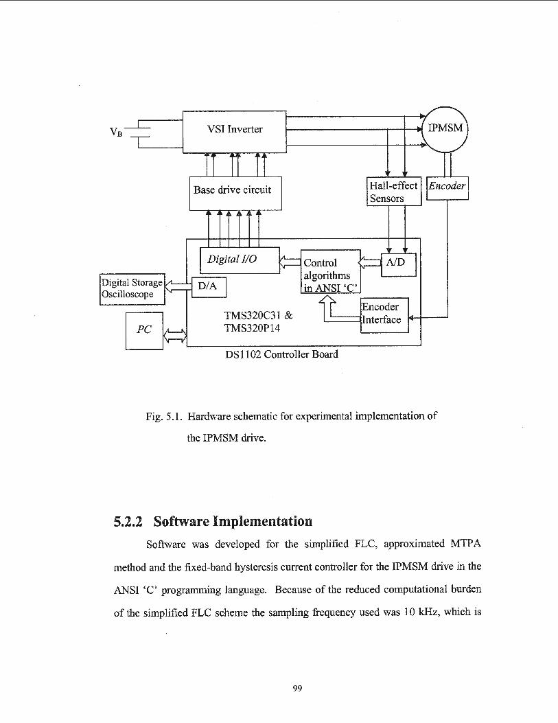
Vs I VSI Inverter i IPMSM \
rr n rr Base drive circuit Hall-effect ~Encoderl
Sensors ~ ~ ~ ~ ~ ~ J
b== Control ~AID Digital 110 I Digital Storage _/1--- DIA I
algorithms
Oscilloscope "-r- in ANSI 'C'
it Encoder TMS320C31 & Interface
PC ;L--J\ TMS320P14 \r-,1
DS 1102 Controller Board
Fig. 5.1. Hardware schematic for experimental implementation of
the IPMSM drive.
5.2.2 Software Implementation
Software was developed for the simplified FLC, approximated MTP A
method and the fixed-band hysteresis current controller for the IPMSM drive in the
ANSI 'C' programming language. Because of the reduced computational burden
of the simplified FLC scheme the sampling frequency used was 10 kHz, which is
99

adequate for successful real-time implementation of the drive. The detailed
software implementation is described below.
Step 1: All the peripherals of the DSP board are initialized in order to access the
on-board peripherals. Macro functions supplied with the DS 1102 controller board
achieve this task. The macro function in itO initializes the D/ A converter subsystem
of the DS 1102 for output. This command also resets the interrupt request bits and
calibrates the 16-bit AID converters. The functions timerOO and timer 1 () are used
to initialize the DS 1102-TMS320C31 's on-chip timers to generate timer interrupts
at a predefined sampling rate as given in Table I. This is essential for real-time
implementation. The detailed initialization and the I/0 functions for the AID
converters and 16 bit I/0 ports can be obtained from the reference manual of the
DS1102 [71].
Table 1: Peripheral initialization
void main() {
init (); / * i n i t DAC mode, calibrate ADCs */ i nit_slave_DSP_digital_i_o();
/* initialize i / o ports for output* / *error=NO ERROR;
/* initiali ze overload error flag */ dp_ mem[O] .f=O. O;
/ * init 1st dp-mem loc for float */ dp mem[l] .f=O.O;
-/* ini t 2nd dp_mem loc f or f l oat */ d sll02_in c_cl ear_ counter(l);
/* c l ear i ncr. encod e r counter */ start i s r tO(TS);
/*-initialize sampling clock timer */ while (*e rror==NO_ ERROR);
/* background process * /
100
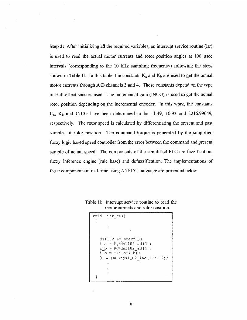
Step 2: After initializing all the required variables, an interrupt service routine (isr)
is used to read the actual motor currents and rotor position angles at 100 J..LSec
intervals (corresponding to the 1 0 kHz sampling frequency) following the steps
shown in Table II. In this table, the constants Ka and Kb are used to get the actual
motor currents through AID channels 3 and 4. These constants depend on the type
of Hall-effect sensors used. The incremental gain (INCG) is used to get the actual
rotor position depending on the incremental encoder. In this work, the constants
Ka, Kb and INCG have been determined to be 11.49, 10.93 and 3216.99049,
respectively. The rotor speed is calculated by differentiating the present and past
samples of rotor position. The command torque is generated by the simplified
fuzzy logic based speed controller from the error between the command and present
sample of actual speed. The components of the simplified FLC are fuzzification,
fuzzy inference engine (rule base) and defuzzification. The implementations of
these components in real-time using ANSI 'C' language are presented below.
Table II: Interrupt service routine to read the motor currents anc1 rotor nosition .
void i s r _tO () {
}
dsl102_ad_star t (); i _a = Ka*ds 1102_ad( 3 ); i_b = Kb*dsl102_ a d( 4 ); i _ c = - ( i _ a +i _b ); 9r = INCG* d s11 02_i n c (l or 2 ) ;
101

Step 3 (Fuzzification): The normalized values of the inputs door and de are passed
to the fuzzification stage which uses pre-selected membership functions to convert
the crisp values of doom ( cvalue) to its corresponding fuzzy value fvalue. In this
work, the trapezoidal and triangular membership functions as developed in chapter
2 are used to reduce the computational burden in real-time.
In order for fuzzification, a routine (Fuzzy) for a singleton fuzzifier is
written in 'C' language as shown in Table III. In this table, the term NS is the
number of fuzzy sets, cvalue is the crisp value, fvalue is the fuzzy value for a
particular input, i denotes the i-th fuzzy set of a particular input, b _1 is the bottom
low value, t_l is the top low value, t_h is the top high value, b _h is the bottom high
value and cent is the centroid of a trapezoidal membership function.
Table III: 'C' code for fuzzification.
for(i=O; i<NS; i++) { fvalue[i] = 0;
}
if((cvalue >= b_l[i]) && (cvalue < t_ l[i])) fvalue[i] = (cvalue- b_ l[i])/(t_ 1[i] - b_1[i]); else
{ if((cvalue >= t_ 1[i]) && (cvalue <= t_h[i]))
fvalue[i] = 1; else
{ if (( cvalue > t_ h[i]) && ( cvalue <= b _ h[i]))
fvalue[i] = (cvalue- b_h[i])/(t_h[i]- b_h[i]);
if ( cvalue < cent[ OJ) fvalue[O] = 1;
else { if ( cvalue > cent[NS-1])
fvalue[NS-1] = 1;
102

Step 4 (Fuzzy inference engine - rule base): The fuzzy inference engine is
composed of a set of conditional ("if-then") statement control rules that obtain the
results of all applicable rules. In the case of the simplified FLC, it computes the
fuzzy value of the output based on a single fuzzy input. This is a highly simplified
form of fuzzy rule inference as there are no AND or OR statements. The routine
for the fuzzy inference engine (FuzzyEngine) is written in 'C' language as given in
Table IV. In this table, NSl (=5) and NS2 (=5) are the number of fuzzy sets for
dCOm, and iqn*, respectively.
Table IV: 'C' code for rule evaluation.
for (i=O; i<NS2; i++) fvalue2[i] = 0.0;
for (j=O; j<NS 1; j++) { minval = fvalue[j]; fvalue2[j] = minval; }
Step 5 (Defuzzification): The input for the defuzzification process is a fuzzy set
and the output is a single number, which is non-fuzzy (i.e., a crisp value). In order
to reduce the computational burden for on-line implementation the following
mathematical form is obtained using the center of gravity method [72],
103

NS
IAj *~cj (i)*Centj . j=l 1 = ~--N-S ___ _ (5.1)
IAj j=l
where Aj is the area , Centj is the centroid of the jth output set Cj, NS is the number
of output fuzzy sets, ~c (i) is the fuzzy value which scales the output set Cj. J
According to the above mathematical formula, a new routine for
defuzzification has also been written in 'C' language as given in Table V.
Table V: 'C' code for center of area defuzzification.
tempi= 0; cvalue2 = 0.0; for (i=O; i<NS3; i++)
{
}
temp2 = fvalue2[i]*areas_2[i]; cvalue2 += temp2*cent_2[i]; temp 1 += temp2;
cvalue2 /= temp 1;
TEC = KI * cvalue2;
where areas_2[i] is the area, cent_2[i] is the centroid of the ith fuzzy set of the
output.
After finishing the FLC calculations the command currents ia*, ib* and i/ are
generated from the command torque T e * and the rotor position angle 8r using the
inverse Park's transformation. These command phase currents are compared with
the actual motor currents in the hysteresis current controller, which provides the
104

necessary driving pulses for the inverter switches. The hysteresis current controller
algorithm is also written in 'C' language. The digital I/0 ports are configured as
output ports for the six PWM logic pulses, which are fed to the base-drive circuit of
Inverpower 3-phase voltage source inverter module No. Plll . For the sake of
simplicity, the steps 1-5 are summarized in the flow chart of Fig. 5.2 .
...__-t Calculate command & reference currents
Fig. 5.2. Flow chart of the software for real-time implementation of the FLC based
IPMSM drive.
105

Finally, the program is compiled by the TIC compiler and downloaded to
the DSP board using dSPACE loader program down1102.
5.3 Experimental Results and Discussion
Please note that in the following experimental results, unless otherwise
noted, the time scale for speed responses is 0.5 seconds per horizontal division, for
a full-graph time span of 5 seconds. The time scale for simulated tests was either
1.0 or 0.5 seconds for full-graph time span. This difference is due to the
operational nature of the manually operated experimental setup. The results reveal
that the experimental startup responses are not as rapid as the simulation results
would indicate. This is because the experimental setup dictates that voltage be
applied to the inverter manually in a ramp-like fashion and not instantaneously as is
the case with simulation.
The speed response and corresponding actual 'a' phase current for the
simplified FLC based/MTPA IPMSM drive are shown in Figs. 5.3 (a) and (b),
respectively, for no load and rated speed (188.5 rad./sec.) conditions. The results
show that the drive achieves the command speed very promptly, with no observable
overshoot or oscillation, and follows command speed accurately. Steady-state error
appears to be zero. Phase current is within the rated values of the machine.
Figures 5.4 (a) and (b) show the speed response and actual phase current,
respectively, for the simplified FLC based/MTP A IPMSM drive at rated load and
rated speed conditions. Again the drive follows the command speed without
detectable steady-state error, and achieves this quickly with no observable
overshoot or oscillation. Again, phase current is within the rated values of the
machine, but has increased slightly from the lightly loaded case.
106

Figures 5.5 (a)-(c) show the speed response, q- and d-axis command
currents and actual phase current, respectively, for the simplified FLC
based/MTPA IPMSM drive at light load and low speed (90 rad./sec.) conditions.
Here, it can be seen that the drive follows the command speed promptly, without
overshoot and no visible steady-state error. As in the simulated case, ~ * appears to
be a scaled opposite of iq *. The phase current remains within rated values of the
machine. These results verify that the FLC based/MTP A IPMSM drive can quickly
achieve, and precisely follow, command speed under various loading conditions.
The responses of the simplified FLC based/MTP A IPMSM drive to sudden
changes in command speed at light load conditions are shown in Figs. 5.6 (a) to (c).
It is demonstrated that the drive can follow the command speed quickly and
accurately during a step increase (90 rad./sec.~188.5 rad./sec.) and decrease (188.5
rad./sec.~125 rad./sec.) of speed under light load conditions and also under rated
load conditions (80 rad./sec.~165 rad./sec. and 165 rad./sec.~80 rad./sec.). There
are no detectable over- or undershoots or steady-state errors. Figure 5.6 (c)
illustrates the increase in phase current frequency with increased motor speed. A
software program (Dspeed.c ), included in Appendix D, was used to achieve the
real-time step change of command speed.
The ability of the drive to accommodate sudden changes in load was also
examined experimentally. Figures 5.7 (a)-( c) show the speed response, q- and d
axis command currents and actual phase current at steady-state after loading,
respectively, for the simplified FLC based!MTP A IPMSM drive for a sudden
increase of load (from no load to rated load) at rated speed. It can be seen that the
drive is virtually insensitive to such a load disturbance. Also, ict * appears to be a
107

. * scaled opposite of lq and the phase current remams within rated machine
parameters.
Figures 5.8 (a) and (b) show the speed response and actual phase current, at
steady-state after loading, for the simplified FLC based/MTP A IPMSM drive for a
sudden increase of load (from no load to rated load) at low speed (90 rad./sec.).
Once again, the drive remains detectably insensitive to the load disturbance. These
results indicate that the drive can accommodate sudden increases in load, at varying
speeds, without disturbance of rotor speed and while remaining within the rated
phase currents of the machine.
Therefore, the efficacy and robustness of the simplified FLC based/MTP A
IPMSM are verified.
108
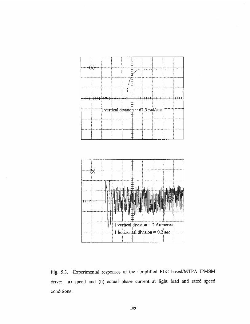
············:---········· 1 vertical ~vision = 67.3 radlsec. ··········T·········· : : :
r:r ; 1: r r ; 1
. 1 vertical division = 2 Amperes : : T : : :
.... 't" 1 horizontal diVision= o.i sec.
Fig. 5.3. Experimental responses of the simplified FLC based!MTPA IPMSM
drive: a) speed and (b) actual phase current at light load and rated speed
conditions.
109

. . . . . . . . •• •••••••• •{-•••• •• ••••••i- •• • • • • • • •• • •~••••• ••• • ••• ~••• •• o o •••• ••• • • • ••• •~•• •• • • •••• • • • :.••••• o ••••u~o ooouoooo o o~o • • ••• • • ••• •
•••••: l)l I :~ ••••• :1 t••ll : ~ : ~=e~c~1viston=~~-~ ~:~·~:j I ············i··················································· ········+ ···········'······················-..l. .......... .
~ j i j i l
Fig. 5.4. Experimental responses of the simplified FLC based!MTPA IPMSM
drive: a) speed and (b) actual phase current at rated load and rated speed
conditions.
110
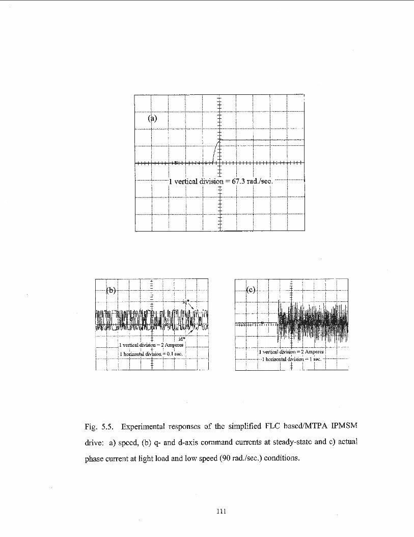
t-
··········*;·· j ·······i j········ tj···jj···j····· ·· · ···· · · · ··i· · ··········t········· · ·- ~· -······ ····i······ ····· ······ · · ··;·· ······ ····-~---··· ·· ·· ··t······ · ····-~---······--·
. ........... !'··, !' .·, i'··, 1' .. ,····· /········+······ j·······i ·········· i············ f.: i i i i
............ j ............ :1 vertical division = 67.3 n!d./se~ .......... 1 .......... ..
frrr r~rrl
-··-(b)r···+ ...... : .... + .......... , ........... , ........... ; ............ : ........... J
··········-t-----.-l---········f···--·
' ' ' ' ... ·t .. "+ id*L. .. :... ... . .... ;... ..f 1 vemcal <livisi~n = ~ Am~eres .!. ........ !.. . .. .
·t ..... J~.-~o..E>~~~~~~~-~-?.-.~.:e.~· . .! ....... . :
Fig. 5.5. Experimental responses of the simplified FLC based/MTPA IPMSM
drive: a) speed, (b) q- and d-axis command currents at steady-state and c) actual
phase current at light load and low speed (90 rad./sec.) conditions.
111

:~<t :J llt+···-····'··-........ l .......... ; ........... ' ............ j ! 1
...... <p.L.L.. i .. .. f ....... + .......... ; .......... + ............ ; ............ ; .......... ~ .... + .. ·-; ..... i ... .. i . 7
Wi! ! !
; i .......... L ......... .l ....... J ........... .L---·····-....... ~ .......... Ti .. ~;t;";;;I·di~on = ss.3 rnd.tsec,: . ·.' i ! !
·········· -~---.--·-···+······ ······i············t .. ···-· ··-······+···········+-·- ······j·····--.. ··j···········
....... t- ........ J . ... J ... r..... -···t · .. ··+ . .. : ....... ;
' ' ........... i ............ t ............ ; ............ i,.......... ·- ···---~---·-····---~---.. ···---i.-......... l ......... .
i I vertical division= 77 8 rad.lsec. ...................... .;. .. ······-i ......... --:----·····
l ! --·-····--t···-------;--··· -·-·r·····-·--r-·--·-
........... L. ....... ) .... :--.. -·! --------··r· .. ··· ··--~---------•••••••• ! • •
speed increased here (c)
1 vertical division = 2 Amperes : : : -t- : : '
f ......... ; ............ .;., horizontal division= 0.1 sec ... ; ........... .;..
Fig. 5.6. Experimental responses of the simplified FLC based!MTPA IPMSM
drive for sudden changes in command speed: a) speed at light load, (b) speed at
rated load (note scale difference) and c) actual phase current at light load
conditions.
112
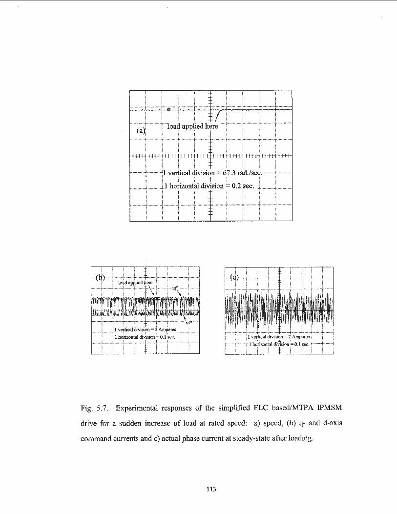
. . . ' ··········-~· -···········r········ · ··- ~ ·- · · · ·······1· ··········
. . . . ...•... ·--~-· ..... ··-·--r ........ · ···~· -··· · ·· · .. - ~···· · · · ··· · · . I . ' '
............ 1. ......... + .. ·1 d li d h ..... L .......... ., ............ , ............ ; .......... .. ( )
! : oa app e ere : : : : a l l 1 l l 1 l l .......... T ......... T ........ T .......... '1' ................... T .......... [ ............ i ........... T ......... .
............ ; ............. fl vertical division= 67.3 rad./sec . ........ j .......... .. ! ! : : t i i i ! ........... + .......... p horizontal division= 0.2
1sec. + ........... j .......... ..
: : . : ; : ~ i . . . ; ! l ........... T ........... f ............ , ........... l ........ .. ........ 1"' ........ T ........... r .......... T ......... ..
· {b}"''';' ''" "''~'""''' i •• ,,.,j,,, ,f•• •••oo!•oooo .,:., i i load applied here ! i !
--·······r· .. -:····· .. ·····1·--....... :........... \ .; ...... ·-··:··---iq~- ·····'·-······
;
.... L. ..... J I ve~cal ~visi?n = ~ Am~eres !.. ........ /. .... _ ' ' 1 honzontu division~ 0.1 :sec. ; !
···-~ ······· : .... t ... -...... .;. ............ 1··-·· ... j .. -· ;
Fig. 5.7. Experimental responses of the simplified FLC based!MTPA IPMSM
drive for a sudden increase of load at rated speed: a) speed, (b) q- and d-axis
command currents and c) actual phase current at steady-state after loading.
113

(a)i . j . . . . . ············ ~- -···· ··· · · --~--- ···u····~- ·· ···· ·· · --~-·· ········ ··· · · ···· ·1·············r······ · ··· · ·~ ·· · ·· ·······1·········· ··
i J lo~d ap~lied here ! ! ! ! ·-----·--··r···---.. ·t···--------l·------ ---- ~""------ .. - ··\··j·······---··"t""··--------r-----·------:------------
. . . . . . . . . . ··········;···········: ············:········-···:············ . . . : : : i j j
.••• r l ;;~~~~;on~~',_~:~~:_:;~,~~:_: : : 1!,_
. ... ........ i,; ............. i,f ............ i,[ ............ i,'........... : : : :
l : ! :
·_·_·_-_-___ c __ ~_-__ ) _._:,,,·--_-_-_ -_-_-_-_-_-_-_ -_ -_1,_,, -_-_-_-_-_-_ -_-_-_-_ -_-_1,,,_-__ .... _. __ .. _-_-_-_ -_·_::,_, _____ --_-_-__ --_-_ -_-_ .......... r ·--··----r------·---r--·----·---r------.. .. . .. ........ j_ .......... --~-...... ...... [ .. ......... l_ . .... ...... .
.. ... .. . !,,_'_ ... ... -:,~ - ... .. .. 'f, . . :. ... . J.n lil.... .. 'f ... ----r ....... ~[f ... . . m ll .
. . .. . . .. . ....... ···' ... .... ··• ··-······ . .; ...... --- -----·. '·· .. .. . ... .. ... ... ... --~----
r ! i ~~;;;~;.) di~o;;;;;1A;;;;;;;:~~r !_
1
----· ......
i i i i I i i i . .......... -y .......... +-1 horizontal division = 0.1 sec. +----·----·+-----------
j ! ! i $ ! ! i i
Fig. 5.8. Experimental responses of the simplified FLC based!MTPA IPMSM
drive for a sudden increase of load at low speed (90 rad./sec.): a) speed, (b) actual
phase current at steady-state after loading.
114

5.4 Concluding Remarks
The detailed DSP based real-time implementation procedure for the
simplified FLC with approximated maximum torque per ampere mode operation
for the IPMSM drive has been presented in this paper. The complete drive has
been implemented, through both hardware and software, using a digital signal
processor board on a laboratory 1 hp interior permanent magnet motor.
The performance of the proposed IPMSM drive has been investigated
experimentally at different dynamic operating conditions such as sudden changes
of command speed and under varying loads. The drive is found to be robust for use
in high performance industrial drive applications. The experimental results have
validated the simulation results presented in chapter 4.
115

Chapter 6
Conclusions
6.1 General
The literature review of chapter 1 has established that, when coupled with
an appropriate controller, the interior permanent magnet synchronous motor
(IPMSM) can be a favourable choice for use in variable speed high performance
electric motor drives. Speed controllers for the IPMSM, however, typically require
knowledge of machine parameters, which, in the case of the IPMSM, are not
constant under dynamic operating conditions. This makes the design of such
controllers cumbersome and imprecise. Fixed gain controllers suffer from
overshoot, undershoot, steady-state error and even instability in their applications
for high performance IPMSM drives. Conventional adaptive controllers require
complex, and usually expensive, hardware and software for their implementation.
The simplified FLC controller coupled with maximum torque per ampere
operation can overcome these problems by providing an adaptive speed controller
which can accommodate parameter variations, system uncertainties and non
linearities as well as load disturbances while requiring a minimum of computing
116

power and complexity of hardware. This is done through the proposed vector
control scheme of the IPMSM.
Chapter 2 has detailed the analysis and modeling of the pulse-width
modulated (PWM) voltage source inverter (VSI) fed IPMSM drive. Included in
this chapter is a new method for incorporating the maximum torque per ampere
(MTPA) mode of operation in real-time for the IPMSM.
The development of the fuzzy logic controller for the IPMSM drive,
including the concepts of fuzzy logic, linguistic variables, fuzzy sets, membership
functions, fuzzification, fuzzy rule evaluation, and defuzzification, have been
included in the chapter 3. Also, a simplified FLC based speed controller has been
presented.
Chapter 4 presents the comparative simulation results of both a
conventional FLC based IPMSM drive with id * = 0 and the proposed simplified
FLC based drive with id :;:. 0 incorporating the MTP A mode of operation. It is to be
noted that the latter mode of operation is most suitable for practical IPM motor
drive systems. Extensive simulations have verified that the proposed drive can
outperform the conventional FLC based controller with regards to speed response,
current minimization and robustness, with reduced computational burden and need
for high-end hardware.
In chapter 5 the real-time implementation of the new simplified FLC with
MTP A in the IPMSM drive has been presented. Experimental investigation of the
proposed drive under varying dynamic operating conditions has verified that the
drive can achieve and follow command speed promptly without over- or
undershoot and virtually zero steady-state error for a variety of operating
conditions. The robustness of the controller has been verified.
117

6.2 Major Contributions of this Work
• The practical, real-time implementation of the maximum torque per ampere
mode of operation of the IPMSM has been developed.
• A new FLC based controller has been developed for the IPMSM for
operation in the MTP A mode. This controller has been purposefully
simplified so as to reduce computational burden while maintaining high
performance standards.
• The proposed FLC drive with id * 0 has been simulated along with a
conventional FLC drive with id * = 0 for comparison purposes. These
comparative simulations have illustrated the ability of the proposed
controller to handle ever-changing motor dynamics as well as non-linear
load disturbances.
• The proposed simplified FLC/MTP A has been implemented in real-time
through a laboratory 1 hp IPMSM using a digital signal processor controller
board. The efficacy and robustness of the drive has been verified by
experimental investigation of the performance of the drive under various
dynamic operating conditions such as sudden changes in command speed
and loading.
118

6.3 Future Direction of Research
It has been established that the FLC is insensitive to changes in motor
parameters. However, in the development of the maximum torque per ampere
mode of operation the q- and d-axis reactances, Lq and Ld have been assumed to be
constant. Of course, this assumption does not hold true under changing operating
conditions. Although any negative impact appears to be not very significant for
typical uses, it should be further investigated in the context of high performance
adjustable speed drive requirements. In the future, some form of adaptive
technique, such as artificial neural networks or further FLC and neuro-fuzzy
implementations, should be used to accommodate these changes in reactance
parameters.
6.4 Conclusions
• The maximum torque per ampere technique using Taylor senes
approximation can be used in the high performance IPMSM drive for
operating speeds under rated conditions. This allows the motor to develop
maximum mechanical torque with minimum values of stator currents.
• The proposed drive can be used effectively for accurate, precise and robust
speed control of the IPMSM under different dynamic operating conditions
such as, command speed change, load change, system uncertainties and
parameter variations.
119

• The proposed drive provides an adaptive, intelligent control technique for
the IPMSM with minimal complexity, computational burden and hardware
requirement.
• The efficacy of the new control system has been established both
theoretically and experimentally.
120
References
[1] P. C. Sen, "Electric Motor Drives and Control- Past, Present and Future",
IEEE Trans. on Industrial Electronics, vol. 37, no. 6, Dec. 1990, pp. 562-
575.
[2] M. A. Rahman, "Modem Electric Motors in Electronic World",
IEEEIIECON'93 Conference Record, (Hawaii), pp. 644-648.
[3] G. R. Siemon, Electric Machines and Drives, Addison-Wesley Publishing
Company, 1992.
[4] B. K. Bose, Power Electronics and AC Drives, Englewood Cliffs, NJ: Pren
tice Hall, 1986.
[5] P. C. Sen, Principles of Electric Machines and Power Electronics, New
York: Wiley, 1988.
[6] M. H. Rashid, Power Electronics-Circuits, Devices and Applications,
Englewood Cliffs, NJ: Prentice Hall, 1996.
[7] F. Blaschke, "The Principle of Field Orientation as Applied to the New
Transvector Closed-Loop Control System for Rotating Field Machines",
Siemens Review, Vol. 34, May 1972, pp. 217-220.
121

[8] M. A. Rahman, "Permanent Magnet Synchronous Motors - A Review of the
State of Design Art", Proceedings of International Conference On Electric
Machines, Athens, 1980, pp. 312-319.
[9] K. Hasse, "On the Dynamic Behaviour of Induction Machines Driven by
Variable Frequency and Variable Voltage Sources", ETZ A, Bd. 89, H.4, pp.
77-81, 1968.
[10] M.A. Rahman, T. S. Radwan, A.M. Osheiba and A. E. Lashine, "Analysis
of Current Controllers for Voltage Source Inverters", IEEE Trans. Ind.
Electronics, vol. 44, Aug. 1997, pp. 477-485.
[11] H. Le-Huy, K. Silmani and P. Viarouge, "Analysis and Implementation of a
Real-Time Predictive Current Controller for Permanent Magnet Synchro
nous Servo Drives", IEEE Trans. on IEEE Trans. on Industrial Electronics,
vol. 4 1, no. 1, Feb. 1994, pp. 110-117.
[12] H. Le-Huy and L. A. Dessaint, "An Adaptive Current Control Scheme for
PWM Synchronous Motor Drive: Analysis and Simulation", IEEE Trans.
on Power Electronics, vol. 4, no. 4, Oct. 1989, pp. 486-495.
[13] A. Tripathi and P. C. Sen, "Comparative Analysis of Fixed and Sinusoidal
Band Hysteresis Current Controllers for Voltage Source Inverters", IEEE
Trans. on Ind. Electronics, vol. 39, Feb. 1992, pp. 63-73.
122

[14] D. M. Brod and D. W. Novotny, "Current Control ofVSI-PWM Inverters",
IEEE Transactions on Indusfly Applications, Vol. IA-21, No.4, May/June
1985, pp. 562-570.
[15] J. Holtz and S. Stadtfeld, "A Predictive Controller for the Stator Current
Vector of the ac Machines fed from Switching Voltage Source", Proc. Int.
Power Engineering Conf, Tokyo, Japan, Apr. 1983, pp. 1665-1675.
[16] A. B. Plunkett, "A Current Controlled PWM Transistor Inverter Drive",
Conf. Rec. IEEE-lAS Annu. Meeting, Oct. 1979, pp. 951-957.
[17] M. N. Uddin, T. S. Radwan, G. H. George and M. A. Rahman, "Perform
ance of Current Controllers for VSI-Fed IPMSM Drive", IEEE Transac
tions on Industry Applications, Vol. 36, No.6, Nov./Dec. 2000, pp. 1531-
1538.
[18] B. K. Bose and P. M. Szczesny, "A Microcomputer-Based Control and
Simulation of an Advanced IPM Synchronous Machine Drive System for
Electric Vehicle Propulsion", IEEE Trans. on Industrial Electronics, vol.
3, no. 4, Nov. 1988, pp. 547-559.
[19] A. V. Gummaste and G. R. Siemon, "Steady State Analysis of a Permanent
Magnet Synchronous Motor Drive with Voltage Source Inverter", IEEE
Trans. on Industrial Applications, vol. IA-17, no. 2, March/April 1981 ,
pp.143-151.
123

[20] G. R. Siemon and A. V. Gummaste, "Steady State Analysis of a Permanent
Magnet Synchronous Motor Drive with Current Source Inverter", IEEE
Trans. on Industrial Applications, vol. IA-19, no. 2, March/April 1983, pp.
190-197.
[21] T. H. Liu, C. M. Young and C. H. Liu, "Microprocessor Based Controller
Design and Simulation of Permanent Magnet Synchronous Motor Drive",
IEEE Trans. on Industrial Electronics, vol. 35, no. 4, Nov. 1988, pp. 516-
523.
[22] P. Pillay and R. Krishnan, "Modeling of permanent magnet motor drives",
IEEE Trans. on Industrial Electronics, vol. 35, no. 4, Nov. 1988, pp. 537-
541.
[23] P. Pillay and R. Krishnan, "Modeling, Simulation and Analysis of Perma
nent Magnet Motor Drives, Part I: The Permanent-Magnet Synchronous
Motor Drive", IEEE Trans. on Industry Applications, vol. 25, no. 2,
March/April1989, pp. 265-273.
[24] P. Pillay and R. Krishnan, "Modeling, Simulation and Analysis of a High
Performance Vector Controlled Permanent Magnet Synchronous Motor
Drive", IEEEIIAS Annual Meeting Conference Record, 1987, pp 253-261.
[25] P. Pillay and R. Krishnan, "Control Characteristics and Speed Controller
Design for High Performance Permanent Magnet Synchronous Motor
Drive", IEEE Trans. on Power Electronics, vol. 5, no. 2, April 1990,
pp.151-159.
124

[26] M. A. Rahman, M. Vilathgamuwa, M. N. Uddin & K .J. Tseng, " Non
.linear control of interior permanent magnet synchronous motor drive",
IEEE Trans. on Industry Applications, Vol.39, Mar/April 2003, pp.408-
416.
[27] P. Pillay, C. R. Allen and R. Budhabhathi, "DSP-Based Vector Control and
Current Controllers for Permanent Magnet Synchronous Motor Drive",
IEEEIIAS Annual Meeting Conference Record, Seattle, Washington, 1990,
pp. 539-544.
[28] B. K. Bose, "A High Performance Inverter Fed Drive System of an Interior
Permanent Magnet Synchronous Machine", IEEE Trans. on Industry Ap
plications, vol. IA-24, no. 6, 1988, pp. 987-997.
[29] H. Le-Huy and L. A. Dessaint, "An Adaptive Current Control Scheme for
PWM Synchronous Motor Drive: Analysis and Simulation", IEEE Trans.
on Power Electronics, vol. 4, no. 4, Oct. 1989, pp. 486-495.
[30] H. Le-Huy, K. Silmani and P. Viarouge, "Analysis and Implementation of a
Real-Time Predictive Current Controller for Permanent Magnet Synchro
nous Servo Drives", IEEE Trans. on IEEE Trans. on Industrial Electronics,
vol.41,no.1,Feb.1994, pp.l10-117.
[31] B. K. Bose and P. M. Szczesny, "A Microcomputer-Based Control and
Simulation of an Advanced IPM Synchronous Machine Drive System for
125

Electric Vehicle Propulsion", IEEE Trans. on Industrial Electronics, vol.
3, no. 4, Nov. 1988, pp. 547-559.
[32] T. M. Jahns, G. B. Kilman and T. W. Neumann, "Interior Permanent Mag
net Synchronous Motors for Adjustable Speed Drives", IEEE Trans. on
Industry Applications, vol. IA-22, no. 4, July/August 1986, pp. 738-747.
[33] T. M. Jahns, "Flux-Weakening Regime Operation of an Interior Permanent
Magnet Synchronous Motor Drive", IEEE Trans. on Industry Applications,
vol. IA-23, no. 4, 1987, pp. 681-689.
[34] S. Morimoto, Y. Takeda and T. Hirasha, "Current Phase Control Methods
for Permanent Magnet Synchronous Motors", IEEE Trans. on Power Elec
tronics, vol. 5, no. 2, April1990, pp. 133-139.
[35] S. Morimoto, Y. Takeda, T. Hirasa and K. Taniguchi, "Expansion of Operat
ing Limits for Permanent Magnet Motor by Current Vector Control Con
sidering the Inverter Capacity", IEEE Trans. on Industry Applications, vol.
26, no. 5, Sept./Oct. 1990, pp.866-871.
[36] S. Morimoto, Y. Takeda, K. Hatanaka, Y. Tong, and T. Hirasa, "Design and
Control System of Permanent Magnet Synchronous Motor for High Torque
and High Efficiency Operation", IEEE/IAS Annual Meeting Conference
Record, 1991, pp. 463-468.
[37] S. Morimoto, K. Hatanaka, Y. Tong, Y. Takeda and T. Hirasa, "Servo Drive
System and Control Characteristics of salient Pole Permanent Magnet Syn-
126

chronous Motor", IEEE Trans. on Industry Applications, vol. 29, no. 2,
March!April1993, pp. 338-343.
[38] S. Morimoto, Y. Takeda, and T. Hirasa, "Flux Weakening Control Method
for Surface Permanent Magnet Synchronous Motors", IPEC Conference.
Recor~ Tokyo,Japa~ 1990,pp.942-950.
[39] S. Morimoto, M. Sanda andY. Takeda, "Effects and Compensation ofMag
netic Saturation in Flux-Weakening Controlled Permanent Magnet Syn
chronous Motor Drives", IEEE Trans. on Industry Applications, vol. 30, no.
6, Nov./Dec. 1994, pp. 1632-1637.
[40] M. F. Rahman, L. Zhang and K. W. Lim, "A Direct Torque Controlled Inte
rior Permanent magnet Synchronous Motor Drive Incorporating Field
Weakening", IEEE/IAS Annual Meeting Conference Record, 1997, pp. 67-
74.
[41] S. Vaez, V. I. John and M. A. Rahman, "An On-Line Loss Minimization
Controller for Interior Permanent Magnet Motor Drives", IEEE Trans. on
Energy Conversion, Paper No. PE-!345-EC-0-07-1998.
[42] T. S. Radwan, M.A. Rahman, A.M. Osheiba and A. E. Lashine, "Perform
ance of a Hybrid Current-Controlled VSI Permanent Magnet Synchronous
Motor Drive", IEEEIPESC Conference Record, 1996, pp.951-957.
[43] M.A. Hoque, Casey Butt and M.A.Rahman, "A Novel Approach for MTPA
Speed Control of IPMSM Drive", Proc. 2nd IEEE International Confer-
127

ence of Electrical & Computer Engineering, Dhaka, Dec. 26-27, 2002, pp.
336-339.
[44] R. Krishnan, "Control and Operation of PM Synchronous Motor Drives in
the Field Weakening Region", IEEEIIECON'93 Conference Record, Ha
waii, 1993, pp. 745-750.
[45] S. R. Macminn and T. M. Jahns, "Control Techniques for Improved High
Speed Performance of Interior PM Synchronous Motor Drives", IEEE
Trans. on Industry Applications, vol. 27, no. 5, Sep./Oct. 1991, pp. 997-
1004.
[46] R. Dhanuadi and N. Mohan, "Analysis of Current-Regulated Voltage Source
Inverters for Permanent Magnet Synchronous Motor Drives in Normal and
Extended Speed Range", IEEE Trans. on Energy Conversion, vol. 5, no. 1,
March 1990, pp. 137-147.
[47] A. Kumamoto andY. Hirame, "A Flux-Weakening Method for a Buried
Permanent Magnet Motor with Consideration of Parameter Detunning on
System Performance", IPEC Conference Record, Tokyo, Japan, 1990, pp.
950-955.
[48] I. Choy, T. Yoon, K. Kim, and M. Park, "Microprocessor-Based Permanent
Magnet Synchronous Motor Drives using MRAC", JPEC Conference Re
cor~ Toky~Japan, 1990,pp.481-488.
128

[49] E.Cerruto, A. Raciti and A. Testa, "A Robust Adaptive Controller for PM
Motor Drives in Robotic Applications", IEEE Trans. on Power Electron
ics, vol. 10, no. 1, Jan. 1995, pp. 62-70.
[50] Y. Sozer and D. A. Torrey, "Adaptive Flux Weakening Control of Perma
nent Magnet Synchronous Motors", IEEE/IAS Annual Meeting Conference
Record, 1998,pp.475-482.
[51] C. Namudri and P. C. Sen, "A Servo-Control System using a Self-Controlled
Synchronous Motor (SCSM) with Sliding Mode Controller", IEEEIIAS An
nual Meeting Conference Record, 1987, pp. 283-295.
[52] A. Consoli and Antonio, "A DSP Based Sliding Mode Field Oriented Con
trol of an Interior Permanent Magnet Synchronous Motor Drive", IPEC
Conference Record, Tokyo, Japan, 1990, pp. 263-303.
[53] M. Ghirby and H. Le-Huy, "Optimal Control and Variable Structure Com
bination using Permanent Magnet Synchronous Motor", IEEEIIAS Annual
Meeting Conference Record, 1994, pp. 408-415.
[54] R. B. Sepe and J. H. Lang, "Real Time Adaptive Control of the Permanent
Magnet Synchronous Motor", IEEEIIAS Annual Meeting Conference Re
cord, 1990,pp. 545-552.
[55] M. A. El-Sarkawi, A. A. El-Samahy and M. L. El-Syed, "High Performance
Drive of de Brushless Motors Using Neural Network", IEEE Trans. on
Energy Conversion, vol. 9, no. 2, June 1994, pp, 317-322.
129

[56] C. Shiguo, D. G. Holmes and W. A. Brown, "Digital Control of a Servo
System using Neural Network", IEEEIIAS Annual Meeting Conference
Record, 1995, pp. 129-133.
[57] M. A. Rahman and M. A. Hoque, "On-Line Adaptive Artificial Neural
Network Based Vector Control of Permanent Magnet Synchronous Mo
tors", IEEE Trans. on Energy Conversion, vol. 13, no. 4, 1998, pp. 311-
318.
[58] Y. Yi, D. M. Vilathgamuwa and M. A. Rahman, "A New Artificial Neural
Network Controller for an Interior Permanent Magnet Motor Drive",
IEEEIIAS Annual Meeting, Chicago, 2001, pp. 1115-1120.
[59] M.A. Rahman, M.A. Hoque, C. B. Butt, M. N. Uddin and M.A. Abido,
"Testing of Genetic-PI Based Controller for IPMSM Drive", IEEE Confer
ence on Industrial Technology, Bangkok, Thailand, Dec. 2002, CD-ROM.
[60] K. Inoue, Y. Takakado and M. Nakaoka, "Auto Tuning Technology for
Fuzzy Algorithms Based DC Brushless Servo Systems", IEEE/PESC Con
f erence Record, 1993, pp. 446-450.
[61] K. Erenay, I. Ciprut, L. Tezduyar, Y. Istefanopulos, "Application of Fuzzy
Algorithms to the Speed Control of Washing Machines with Brushless DC
Motors", Proceedings of International Conference on Electric Machines,
Istanbul, Turkey, 1998, pp. 1231-1236.
[62] Z. Koviac, S. Bogdan and P. Cmosija, "Fuzzy Rule-Based Model Refer
ence Adaptive Control of Permanent Magnet Synchronous Motor",
IEEEIIECON Conference Record, 1993, pp. 207-212.
130

[63] M. N. Uddin and M.A. Rahman, "Fuzzy Logic Based Speed Control of an
IPM Synchronous Motor Drive", Journal of Advanced Computational In
telligence, vol. 4, no. 2, 2000, paper #JACI-CCECE-S-05.
[64] M.A. Rahman and Ping Zhou, "Field Circuit Analysis ofBrushless Perma
nent Magnet Synchronous Motors", IEEE Trans. on Ind. Elect., vol.43,
No.2, April 1996, pp. 256-267.
[65] P. C. Krause, Analysis of Electric Machinery, McGraw-Hill Inc., 1986.
[66] T. Sebastian, G. R. Siemon and M. A. Rahman, "Modelling of Permanent
Magnet Synchronous Motors", IEEE Trans. on Magnetics, vol. MAG-22,
no.5, 1986,pp. 129-134.
[67] S. Morimoto, M. Sanda andY. Taketa, "Wide-Speed Operation of Interior
Permanent Magnet Synchronous Motors with High-Performance Current
Regulator", IEEE Trans. on Ind. Applicat.,Vol. 30, July/Aug, 1994,
pp.920-926
[68] L. A. Zadeh, "Outline of a New Approach to the Analysis of Complex Sys
tem and Decision Processes", IEEE Trans. on Syst, Man and Cybern., vol.
SMC-3, 1973, pp. 28-44.
[69] Fuzzy Logic Toolbox User Guide, The Math Works Inc., 1997.
131

[70] M. A. Rahman and M. A. Hoque, "On-Line Self-Tuning ANN Based Speed
Control of a PM DC Motor", IEEEIASME Trans. on Mechatronics, vol. 2,
No.3, Sept. 1997, pp. 169-178.
[71] DS1102 Program Loader User's Guide, dSPACE, Paderborn, Germany,
Ver. 2, 1996
[72] H. T. Nguyen, M. Sugeno, R. Tong and R. R. Yager, Theoretical Aspects of
Fuzzy Control, John Wiley & Sons, Inc., 1995.
[73] S. M. Zeid, Master of Engineering Thesis, Faculty of Engineering and Ap
plied Science, Memorial University ofNewfoundland, Dec. 1998.
[74] M. A. Hoque, Doctor of Philosophy Thesis, Faculty of Engineering and
Applied Science, Memorial University ofNewfoundland, Aug. 1996.
[75] T. S. Radwan, Doctor of Philosophy Thesis, Faculty of Engineering and
Applied Science, Memorial University ofNewfoundland, Aug. 1996.
[76] M. N. Uddin, Doctor of Philosophy Thesis, Faculty of Engineering and Ap
plied Science, Memorial University ofNewfoundland, Aug. 2000.
132

APPENDIX A
IPMSM Parameters
Number of phase = 3
Number of poles = 4
Rated current = 3 A
Rated frequency = 60 Hz
Rated power = 1 hp
Rated input line to line voltage = 208 V
q-axis inductance Lq = 0.07957 H
d-axis inductance Ld = 0.04244 H
Stator resistance per phase rs = 1.93 Q
Inertia constant Jm = 0.003 Kg.m2
Rotor damping constant Bm = 0.0008 (N-m)/rad./sec.
Permanent magnet flux linkage \1/m = 0.314 volts/rad./sec.
Magnet type = Samarium Cobalt
133

APPENDIX B
Simulink Model of IPMSM Drive
In modelling the system in SIMULINK it is necessary to work from the
principle equations governing the IPMSM drive system rather than base the indi
vidual components of the model strictly on the schematic of the vector control
scheme. This is because working in the d-q reference frame necessitates the use of
transformation operations that are not implemented physically in real-world sys
tems. Fig. B. l presents the SIMULINK schematic of the complete current
controlled VSI-fed IPMSM drive system that was developed in this work.
134
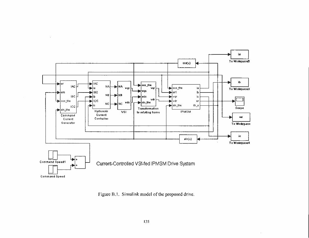
.. r ia I ~ I cos(u) I~ To Workspace6
I I""
r I I I~ I~ lAC .I ib I "'
wr lAC~ I"'
~ cos_the
NA r+ NA LJ.. ia vqs vqr n ---! cos_the ia- To Workspace3 r.._ IBC v qs wr1 ib I"'
wrc
IBC u . r+ ~ ib NB NB
~ vds . vqr ic f----
t..., cos_the ICC vdr h ~ .. vdr wr D ICC u
.. ~
vds sin_the -. r+ ic NC NC ,. sin_the th_e
r+ sin_the T r a nsto rm ati on Scope H-ysteresis VSI to rotating frame IPMSM
Command Current L,.f l WI Current Controller
Generator To Workspace
r I I l --I ic
I sin(u)
I"" To Workspace4
ommand Speed1 l.:-
Current-Controlled VSI-fed IPMSM Drive System r+~f-c
Command Speed
Figure B.l. Simulink model ofthe proposed drive.
135

The following subsections will present the purpose and design of each of
the component blocks of the model in detail. Only the simplified FLC/MTP A
scheme will be addressed.
B.l Command Current Generator
The Command Current Generator block generates the command currents
necessary to maintain the desired rotor speed of the motor. To do this, rotor speed
and rotor angular position are necessary inputs. The schematic of the Command
Current Generator block is shown in Figs. B.2a and B.2b.
The command torque necessary to achieve the desired rotor speed is calcu
lated from the difference between the command speed and the actual speed of the
rotor by the FLC. This command torque is then used to obtain it by means of
Eqn. 2.40. it is then used to attain i/ by Eqn. 2.39. Then, using the appropriate
transformations, ia, ib, and ic are found. This block is shown in Figs. B.2a and B.2b.
B.2 Current Controller
The next block in the model represents the controller for the voltage source
inverter. The current controller takes as input the three phase command currents
from the Command Current Generator and outputs the logic variables NA, NB and
NC used to control the VSI. A fixed band hysteresis controller, as shown in Fig.
B.3, is employed.
136

Command Current Generator
Figure B.2a. Command current generator block.
137
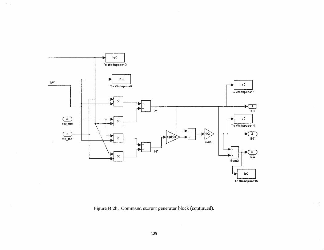
idr"
3
cos_ the
4
sin_the
To Wolkspace10
To Wolkspace9
iq"
Figure B.2b. Command current generator block (continued).
138
lAC
To Wolkspace14
IBC
To Wolkspace15

la--------~~• ~----------~ -.&
lc -----------+---r~~
Command currents
Actual currents
~:.l
~N:3 ~----------~--~~ N5
N2
Fig. B.3. Hysteresis current controller.
139

B.3 Voltage Source Inverter
The next block in the model represents the voltage source inverter and is
designed according to the following equations,
[
v ] [2 - 1 -1] [NA] v: =i -1 2-1 NB V8
v -1 -1 2 NC c
(B. l )
and Eqn. 2.11. Outputs are the vq* and v/ command voltages. This block is shown
in Fig. B.4.
B.4 Transformation to Rotating Frame
The IPMSM model equations require iq r* and id r* to give the outputs COr and
9r. Therefore, v q * and v d *, as obtained from the VSI, must be transformed to the
rotating d-q frame in order to give Vq r* and vd r*. This is done, as shown in Fig. B.5,
using Eqn. 2.12.
NB
3 NC
Voltage Source Inverter
Fig. B.4. Voltage source inverter block.
140

Transformation to Rotating Frame
Fig. B.S. Transformation to rotating reference frame block.
B.5 IPMSM
1 r* r* d This block (Fig. B.6) represents the actua motor. Inputs are Vq , Vct an
ror. In addition, v / and vi* must be converted to i/ and i/ for use in the equa
tions governing the motor dynamics, and this conversion requires the input of cos9r
and sin9r.
Because several functions are performed in this block, it is further com
posed of three sub-blocks which each perform specific tasks.
141
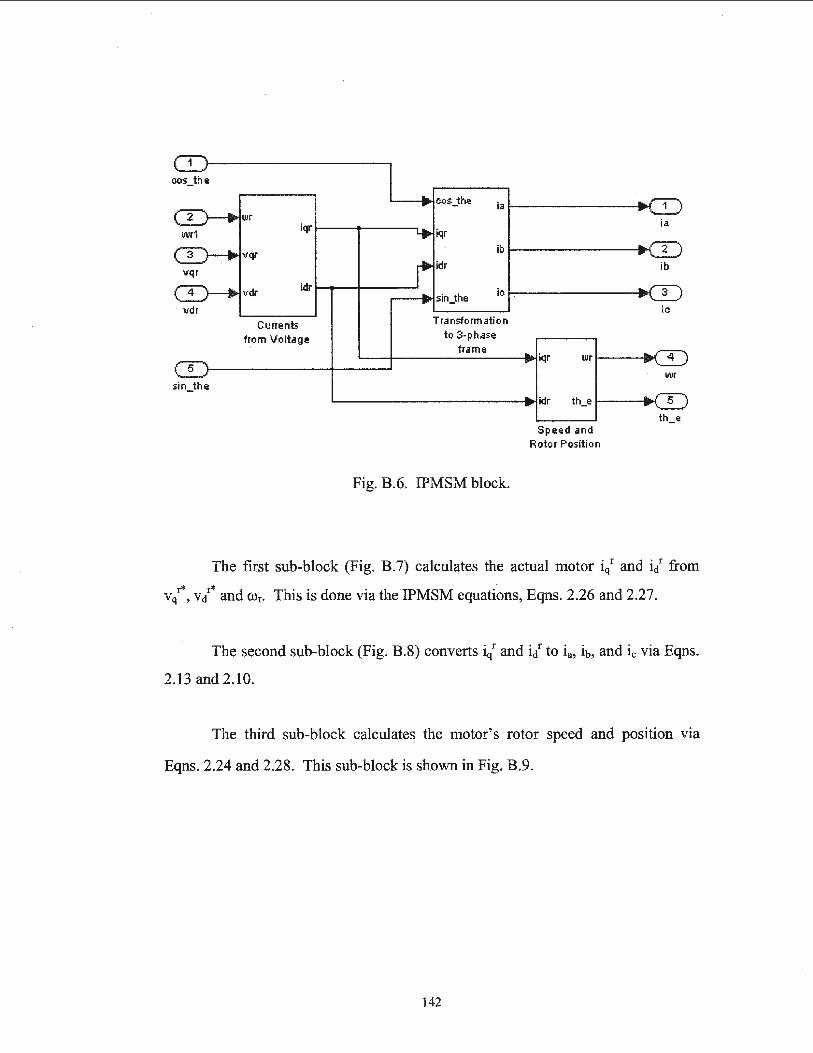
cos_the
vdr
sin_ the
iqr 1----------.
idr 1----+-----l
Currents from Voltage
Transformation to 3-phase
frame
Fig. B.6. IPMSM block.
Speed and Rotor Position
ia
ib
ic
th_e
The first sub-block (Fig. B.7) calculates the actual motor iq1 and ii from
vt, vt and ffir. This is done via theiPMSM equations, Eqns. 2.26 and 2.27.
The second sub-block (Fig. B.8) converts iq1 and ii to ia, ib, and ic via Eqns.
2.13 and 2.10.
The third sub-block calculates the motor' s rotor speed and position vta
Eqns. 2.24 and 2.28. This sub-block is shown in Fig. B.9.
142

2
vqr 3
vdr
Ld
iqr
idr
tator Resistance multiplier
Lq multiplier
Fig. B.7. Calculation of q- and d-axis currents from q- and d-axis command voltages.
143

Transformation to 3-phase Frame
Fig. B.8. Calculation stator currents from q- and d-axis currents.
144

2
idr
l..q multiplier
psi_m
Load
wr
Jm multiplier
Bm
IPMSM
Fig. B.9. Motor speed and position sub-block.
145
APPENDIX C
IGBT Inverter
The insulated gate bipolar transistor (IGBT) has the advantages of both the
bipolar junction transistor (BJT) and metal-oxide-semiconductor field-effect tran
sistor (MOSFET). Because the IGBT has a high input impedance, like a MOSFET,
the gate draws a very small leakage current. So, even though it has low conduction
losses like a BJT, it doesn't suffer from second breakdown problems as do BJTs.
The IGBT is a voltage-controlled device, like a power MOSFET, however,
its performance is closer to that of a BJT than a MOSFET. The IGBT has lower
switching and conduction losses than the MOSFET while sharing many of its ap
pealing features such as ease of gate drive, high peak current capability and rug
gedness. IGBT maximum switching frequencies are higher than BJTs but slower
than power MOSFETs. An IGBT is a three terminal device consisting of a gate,
collector and emitter terminal. Current and voltage ratings of an IGBT can be up to
400 A, 1200 V with a switching frequency of up to 20 kHz.
The schematic of the IGBT inverter module with its snubber circuit is
shown in Fig. C.l. Although the IGBT is capable of handling both soft and hard
switching a snubber circuit has been used to limit the rate of change of voltage
across the inverter legs because of unpredictable transient behavior of the IPMSM.
146

R=25 n, sow
C = 450 ~F. 450 V (de)
_j D1 _j D3 Ds R
Va.
VB vb Vc
D4 _j _j D2
Fig. C.l. Basic circuit of an IGBT inverter module.
147

C.l Base Drive Circuits
The main function of the base drive circuit is to generate six pulses having
proper voltage levels for the six IGBTs of the VSI. In order to operate the IGBTs
as switches, the gate voltages must be such that the IGBTs are into the saturation
mode for low on-state voltages. The outputs of the digital 110 subsystem of the
DSP board are six pulses having magnitudes of 5 V. This is not sufficient voltage
to be used as gate signals to drive the IGBTs and amplification is required. In addi
tion, isolation is needed between the logic circuits and the IGBTs because logic
signals should be applied between the gates and the emitters of the IGBTs. This
means that for the transistors of the upper legs (Tl, T3 and T5), the ground of the
logic pulses will not be common. Therefore, a base drive circuit is needed to pro
vide isolation and appropriate voltages to the gates of the IGBTs in the inverter.
The base drive circuit, which was in the Power Research Laboratory of
M.U.N., is shown in Fig. C.2a and C.2b. The SN7407N chip has been used as a
level shifter that shifts the voltage level from +5V to + 15V. The HP2531 chip is an
optocoupler, which has been used to provide isolation between the logic circuit and
the power circuit of the inverter. The IR2130 chip is the main driver, which pro
vides six driving pulses for the six switches of the inverter. In order to provide
+20V isolated power to the optocoupler and the driver an isolated power supply has
been built, which is shown in Fig. C.2b.
148

Resistance and capacitor values:
R1s-23 = 22 0 , R12-11 = 680 0 , Rs-Jo = 3.3 0, R11 = 3.3 k Q
C3-s = 10 J.tF, C6-11 = 180 pF, C12 =100 J.tF, C13 = 47 J.tF
From SN 7407N
6
+20V
Rll
28
2 27
3 26
4 25
5 24
6 23
7 22
8 IR2130 21
9 20
10 19
11 18
12 17
13 16
14 15
Fig. C.2a. Base drive circuits for the VSI.
149
Output Logic Signals
1
Gl
2
3
G3
4
5
G5
6 Rw
Low side ground
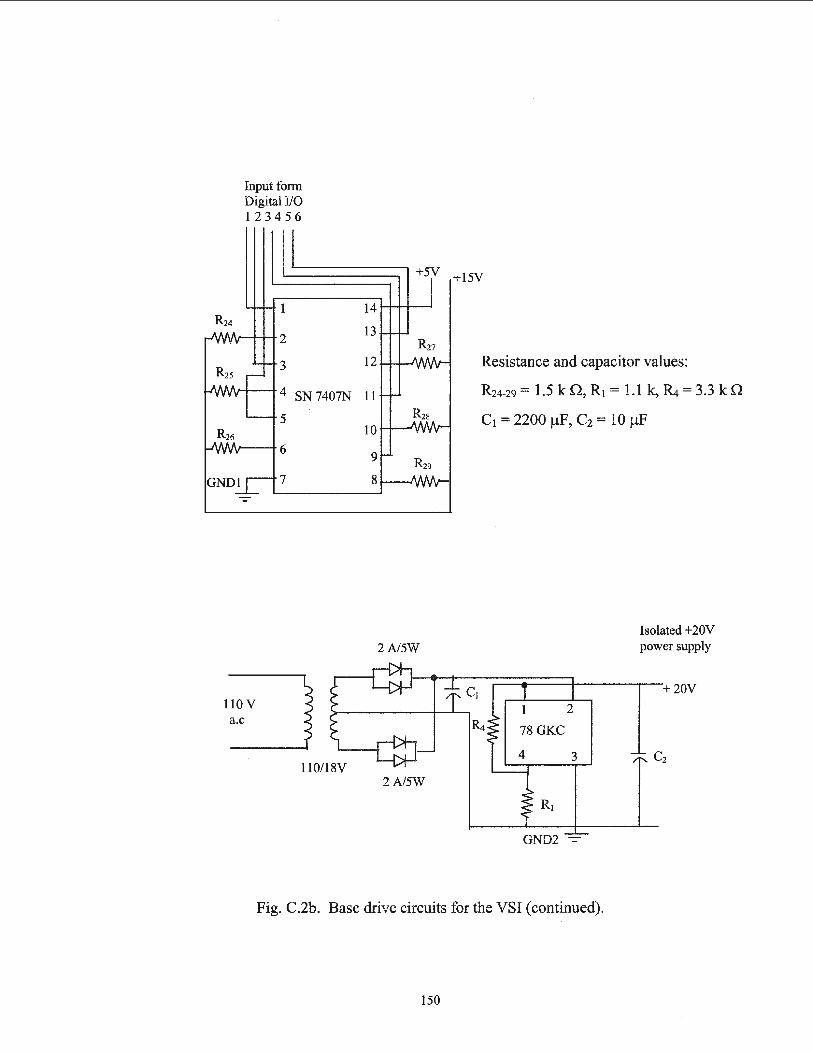
R24
Input form Digital I/O 1 23456
1
2
3
4 SN7407N
5
+5V +15V
14
13 R27
12 Resistance and capacitor values:
11 Rz4-29 = 1.5 k n, R1 = 1.1 k, ~ = 3.3 k n
10 C1 = 2200 JlF, Cz = 10 JlF
GND2 -
Fig. C.2b. Base drive circuits for the VSI (continued).
150

APPENDIX D
Dspeed.c
/* dspeed.c *************************************************************
* * * Instruction to compile with Borland C: * bus version: * bee /ml dspeed.c bcdclib.lib
* *
* ************************************************************************/
#include <stdlib.h> #include <stdio.h>
#include <clib.h> /* Host-DSP interface library include file */
#defme DP MEM OFFS 0 /*use first dual-port memory address*/ - -
unsigned int board _ index; float speed,delta _speed; void close_and_exit (int error_code) {
}
DSP _ unregister_ host_app(); exit( error_ code);
void write_ dual _port_ memory (Uint32 address, Ulnt32 value) {
int error; error = DSP _lock_ board(board _index); if( error!= DSP_NO_ERROR) {
printf("Error: can't lock board error = %d.\n\n" ,error); close_ and_ exit( 5);
} error = DSP _write_ dual _port_ memory(board _index, address, value); DSP _unlock_ board(board _index);
151

if(error != DSP_NO_ERROR) {
printf("Error %d writing the DSP board's dual-port memory !\n\n", error);
close_and_exit(5);
void main (int argc, char *argv[]) {
int error;
printf("\n dspeed "change speed reference from key board .. .''\n\n");
if(argc != 2) {
}
printf("Usage: dspeed board\n\n"); exit(l);
error= DSP _register_ host_ app(" dspeed"); if(error != DSP_NO_ERROR){
switch( error){ case DSP DEVICE DRIVER NOT FOUND: - - - -printf("\nDevice Driver not installed.\n"); break;
case DSP _ VXD _NOT_ LOADED: printf("\n Virtual device driver not installed. \n "); break;
case DSP NO FREE HOST APP IDX: - - - - -printf("\nNo free host application index.''); break;
#ifdefNET
#endif
}
}
case DSP _NET_ERROR: printf("\nNetwork error."); break;
default: printf("\nDSP _register_ host_ app: error code %d\n" ,error); break;
exit( I);
error= DSP _board_index(argv[l],&board_index); if( error!= DSP_NO_ERROR) {
}
printf("\nBoard %s not registered, error = %d.\n", argv[ 1 ],error);
close_ and_ exit(2);
152
I* initialize output signal with 0.0 *I write_ dual _port_ memory(DP _ MEM _ OFFS,
DSP _cvt_ieee_to_ti((Float32) 0.0));
I* set output signal to speed *I do{ printf("\n please enter the delta_speed in rpm ... \n"); scanf("%f", &delta_ speed); speed=delta _speed*O.l 04719755; write_dual_port_memory(DP_MEM_OFFS,
DSP _cvt_ieee_to_ti((Float32) speed)); } while (delta_speed!=O.O); printf("Press RETURN to abort .. . \n"); rewind(stdin); getcharO;
I* reset output signal to 0.0 *I write_ dual _port_ memory(DP _ MEM _ OFFS,
DSP_cvt_ieee_to_ti((Float32) 0.0));
close _and_ exit(O);
153