with anisotropic gibbs{thomson law the stefan problem
TRANSCRIPT
Introduction Anisotropic energies and weak formulation Main existence result Computational results
The Stefan problemwith anisotropic Gibbs–Thomson law
Harald Garcke
University of Regensburg
joint with Stefan Schaubeck (Regensburg)
August 2010
Harald Garcke The Stefan problem with anisotropic Gibbs–Thomson law
Introduction Anisotropic energies and weak formulation Main existence result Computational results
Outline
1 Introduction
2 Anisotropic energies and weak formulation
3 Main existence result
4 Computational results
Harald Garcke The Stefan problem with anisotropic Gibbs–Thomson law

Introduction Anisotropic energies and weak formulation Main existence result Computational results
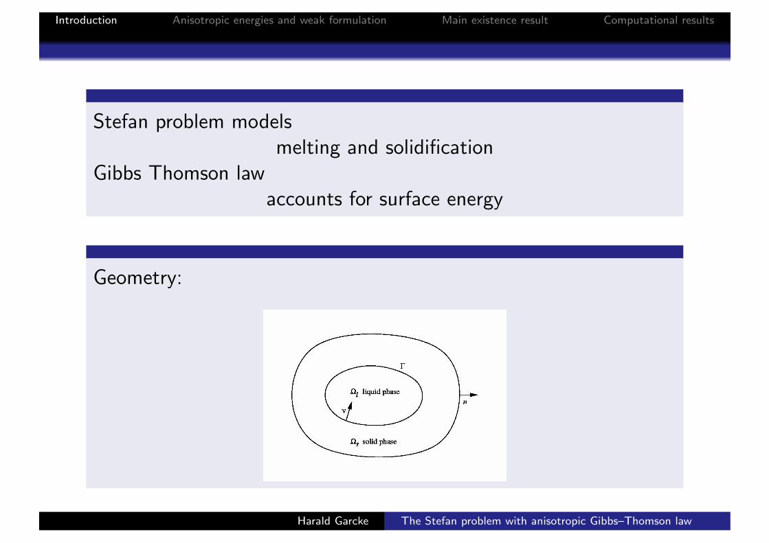
Stefan problem modelsmelting and solidification
Gibbs Thomson lawaccounts for surface energy
Geometry:
Harald Garcke The Stefan problem with anisotropic Gibbs–Thomson law
Introduction Anisotropic energies and weak formulation Main existence result Computational results
Stefan problem modelsmelting and solidification
Gibbs Thomson lawaccounts for surface energy
Geometry:
Harald Garcke The Stefan problem with anisotropic Gibbs–Thomson law

Introduction Anisotropic energies and weak formulation Main existence result Computational results
Mathematical description
Energy balance
∂t(u + χ)−∆u = f weakly !
u : temperatureχ : characteristic function of liquidf : heat sources
Strong formulation:in bulk ∂tu −∆u = f heat equation
on interface Γ V = −[∂u∂ν ] Stefan condition
V : normal velocity[.] : jump across interface
Harald Garcke The Stefan problem with anisotropic Gibbs–Thomson law

Introduction Anisotropic energies and weak formulation Main existence result Computational results
Further condition on interface
Classical condition
u = 0 (= melting temperature)
Physically observed : undercooling (u < 0) in liquid andsuperheating (u > 0) for solid is possible
Reason: Surface energy effects are neglected in classical model
Modified condition
u = H (Gibbs–Thomson law)
H : mean curvature
Harald Garcke The Stefan problem with anisotropic Gibbs–Thomson law

Introduction Anisotropic energies and weak formulation Main existence result Computational results
Issues:
Interfaces do not stay smooth (e.g. topological changes)We need a weak formulation of u = H
u = H describes isotropic surface energyIn nature: surface energies are anisotropic (leads to crystals)
Weak formulation of u = H:
∫ΩT
(∇ · ξ − ∇χ
|∇χ|· Dξ ∇χ|∇χ|
)d |∇χ(t)|dt =
∫ΩT
∇ · (uξ)χdxdt
for all ξ ∈ C∞(ΩT ,Rn) with ξ · n = 0
Harald Garcke The Stefan problem with anisotropic Gibbs–Thomson law

Introduction Anisotropic energies and weak formulation Main existence result Computational results
Important analytical results:
Classical solutions : Chen, Reitich (1992)Radkevich (1992)Escher, Pruss, Simonett (2003)Mucha (2005)
Weak solutions : Luckhaus (1990)Roger (2004)
Idea for the construction of weak solutions (Luckhaus)Use implicit time discretization
All results are for the isotropic case
Harald Garcke The Stefan problem with anisotropic Gibbs–Thomson law
Introduction Anisotropic energies and weak formulation Main existence result Computational results
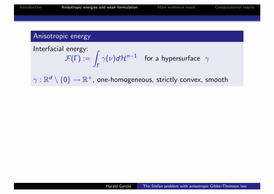
Anisotropic energy
Interfacial energy:
F(Γ) :=
∫Γγ(ν)dHn−1 for a hypersurface γ
γ : Rd \ 0 → R+, one-homogeneous, strictly convex, smooth
First variation
δFδΓ
(Γ)(ξ) =
∫ΓHγ(ξ · ν)dHn−1
with Hγ := ∇Γ · (Dγ(ν))where Dγ is the gradient of γ
Anisotropic Gibbs–Thomson law
u = Hγ , (Gurtin, 1988)
Harald Garcke The Stefan problem with anisotropic Gibbs–Thomson law

Introduction Anisotropic energies and weak formulation Main existence result Computational results
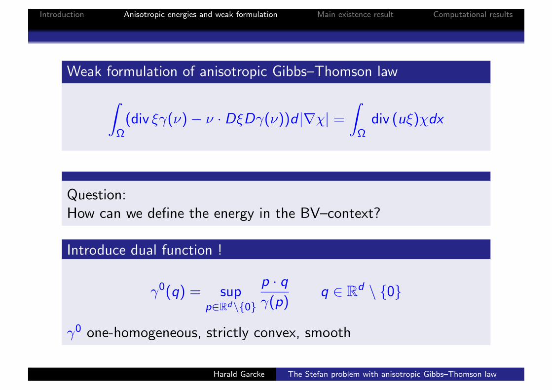
Weak formulation of anisotropic Gibbs–Thomson law∫Ω
(div ξγ(ν)− ν · DξDγ(ν))d |∇χ| =
∫Ω
div (uξ)χdx
Question:How can we define the energy in the BV–context?
Introduce dual function !
γ0(q) = supp∈Rd\0
p · qγ(p)
q ∈ Rd \ 0
γ0 one-homogeneous, strictly convex, smooth
Harald Garcke The Stefan problem with anisotropic Gibbs–Thomson law

Introduction Anisotropic energies and weak formulation Main existence result Computational results
Weak formulation of anisotropic Gibbs–Thomson law∫Ω
(div ξγ(ν)− ν · DξDγ(ν))d |∇χ| =
∫Ω
div (uξ)χdx
Question:How can we define the energy in the BV–context?
Introduce dual function !
γ0(q) = supp∈Rd\0
p · qγ(p)
q ∈ Rd \ 0
γ0 one-homogeneous, strictly convex, smooth
Harald Garcke The Stefan problem with anisotropic Gibbs–Thomson law
Introduction Anisotropic energies and weak formulation Main existence result Computational results
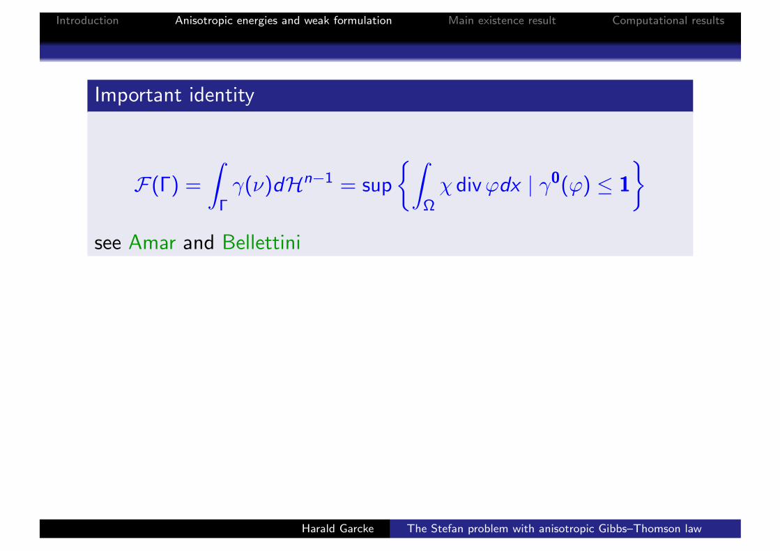
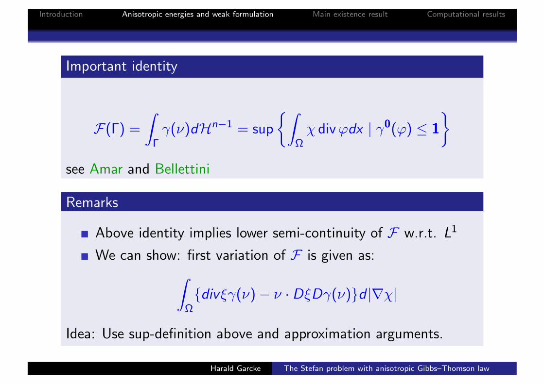
Important identity
F(Γ) =
∫Γγ(ν)dHn−1 = sup
∫Ωχ divϕdx | γ0(ϕ) ≤ 1
see Amar and Bellettini
Remarks
Above identity implies lower semi-continuity of F w.r.t. L1
We can show: first variation of F is given as:∫Ωdivξγ(ν)− ν · DξDγ(ν)d |∇χ|
Idea: Use sup-definition above and approximation arguments.
Harald Garcke The Stefan problem with anisotropic Gibbs–Thomson law
Introduction Anisotropic energies and weak formulation Main existence result Computational results
Important identity
F(Γ) =
∫Γγ(ν)dHn−1 = sup
∫Ωχ divϕdx | γ0(ϕ) ≤ 1
see Amar and Bellettini
Remarks
Above identity implies lower semi-continuity of F w.r.t. L1
We can show: first variation of F is given as:∫Ωdivξγ(ν)− ν · DξDγ(ν)d |∇χ|
Idea: Use sup-definition above and approximation arguments.
Harald Garcke The Stefan problem with anisotropic Gibbs–Thomson law

Introduction Anisotropic energies and weak formulation Main existence result Computational results
Visualize surface energy with the help ofFrank diagram: 1-ball of γ
F = p ∈ Rd | γ(p) ≤ 1Wulff shape: 1-ball of γ0
W = q ∈ Rd | γ0(q) ≤ 1
Isoperimetric characterization
Wulff shape W minimizes surface energy among all surfaces thatenclose the same volume
Frank diagrams and Wulff shapes for different surface energies.
Cubic anisotropy (left) and hexagonal anisotropy (right).
Harald Garcke The Stefan problem with anisotropic Gibbs–Thomson law
Introduction Anisotropic energies and weak formulation Main existence result Computational results
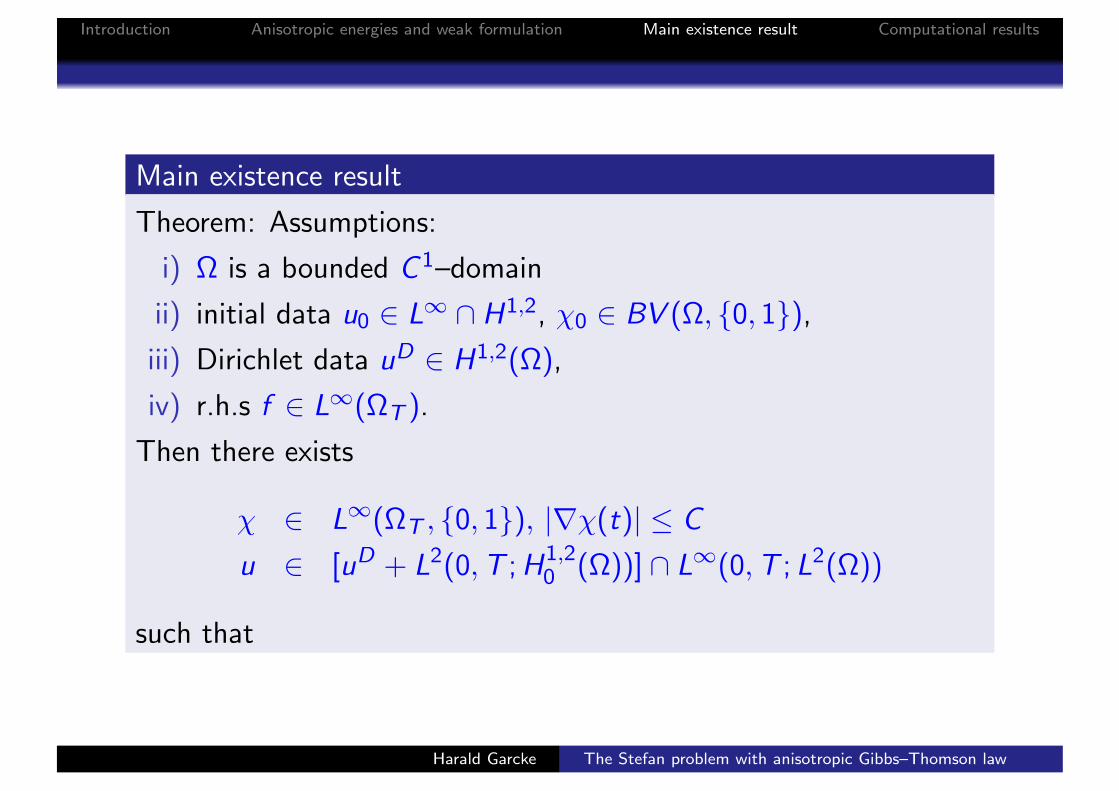
Main existence result
Theorem: Assumptions:
i) Ω is a bounded C 1–domain
ii) initial data u0 ∈ L∞ ∩ H1,2, χ0 ∈ BV (Ω, 0, 1),
iii) Dirichlet data uD ∈ H1,2(Ω),
iv) r.h.s f ∈ L∞(ΩT ).
Then there exists
χ ∈ L∞(ΩT , 0, 1), |∇χ(t)| ≤ C
u ∈ [uD + L2(0,T ; H1,20 (Ω))] ∩ L∞(0,T ; L2(Ω))
such that
Harald Garcke The Stefan problem with anisotropic Gibbs–Thomson law

Introduction Anisotropic energies and weak formulation Main existence result Computational results
Main existence result (continued)
∫ T0
∫Ω(u + χ)∂tϕ+
∫Ω(u0 + χ0)ϕ(0) =∫ T
0
∫Ω∇u · ∇ϕ−
∫ T0
∫Ω f ϕ
for all ϕ ∈ C∞0 ([0,T )× Ω), and∫ T
0
∫Ω
(div ξDγ(ν) · ν − ν · DξDγ(ν)) d |∇χ(t)|dt =
∫ΩT
div (uξ)
for all ξ ∈ C 1(ΩT ,Rd) with ξ · n = 0 on ∂Ω.
Harald Garcke The Stefan problem with anisotropic Gibbs–Thomson law
Introduction Anisotropic energies and weak formulation Main existence result Computational results
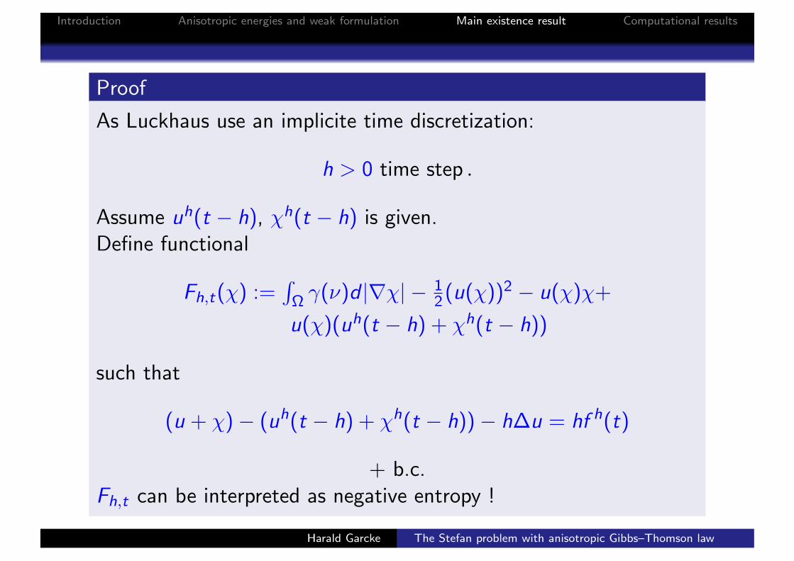
Proof
As Luckhaus use an implicite time discretization:
h > 0 time step .
Assume uh(t − h), χh(t − h) is given.Define functional
Fh,t(χ) :=∫
Ω γ(ν)d |∇χ| − 12 (u(χ))2 − u(χ)χ+
u(χ)(uh(t − h) + χh(t − h))
such that
(u + χ)− (uh(t − h) + χh(t − h))− h∆u = hf h(t)
+ b.c.Fh,t can be interpreted as negative entropy !
Harald Garcke The Stefan problem with anisotropic Gibbs–Thomson law

Introduction Anisotropic energies and weak formulation Main existence result Computational results
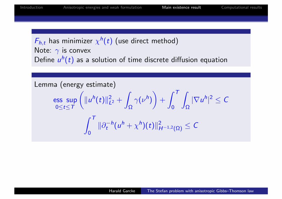
Fh,t has minimizer χh(t) (use direct method)Note: γ is convexDefine uh(t) as a solution of time discrete diffusion equation
Lemma (energy estimate)
ess sup0≤t≤T
(‖uh(t)‖2
L2 +
∫Ωγ(νh)
)+
∫ T
0
∫Ω|∇uh|2 ≤ C
∫ T
0‖∂−h
t (uh + χh)(t)‖2H−1,2(Ω) ≤ C
Proof: Test diffusion equation by uh − uD and use
Fh,t(χhi ) ≤ Fh,t(χh
i−1)
Harald Garcke The Stefan problem with anisotropic Gibbs–Thomson law
Introduction Anisotropic energies and weak formulation Main existence result Computational results
Fh,t has minimizer χh(t) (use direct method)Note: γ is convexDefine uh(t) as a solution of time discrete diffusion equation
Lemma (energy estimate)
ess sup0≤t≤T
(‖uh(t)‖2
L2 +
∫Ωγ(νh)
)+
∫ T
0
∫Ω|∇uh|2 ≤ C
∫ T
0‖∂−h
t (uh + χh)(t)‖2H−1,2(Ω) ≤ C
Proof: Test diffusion equation by uh − uD and use
Fh,t(χhi ) ≤ Fh,t(χh
i−1)
Harald Garcke The Stefan problem with anisotropic Gibbs–Thomson law
Introduction Anisotropic energies and weak formulation Main existence result Computational results
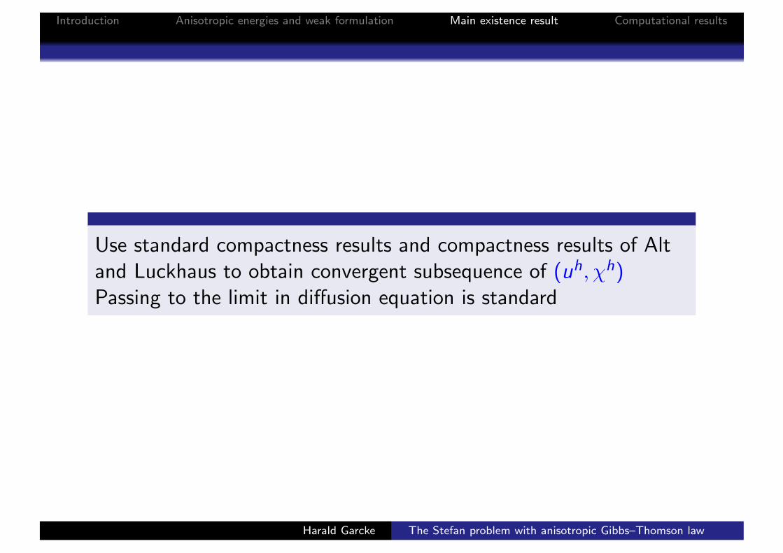
Use standard compactness results and compactness results of Altand Luckhaus to obtain convergent subsequence of (uh, χh)Passing to the limit in diffusion equation is standard
Harald Garcke The Stefan problem with anisotropic Gibbs–Thomson law
Introduction Anisotropic energies and weak formulation Main existence result Computational results
Minima of (χh, uh) of Fh,t fulfills
0 =∫
Ω(div ξDγ(νh(t)) · νh(t)−νh(t) · DξDγ(νh(t)))d |∇χh(t)| −
∫Ω div (uh(t)ξ)χh(t)+ (1)∫
Ω div (L0h(uh(t)− uh(t − h) + χh(t)− χh(t − h))ξ)χh(t)
for all ξ ∈ C∞(Ω,Rd), with ξ · n = 0, where νh(t) = − ∇χh(t)
|∇χh(t)|where v = L0
h(g) is the solutionof v − h∆v = −g in Ω v = 0 on ∂Ω
Goal: Pass to the limit in the discrete Gibbs–Thomson equation (1)
Harald Garcke The Stefan problem with anisotropic Gibbs–Thomson law
Introduction Anisotropic energies and weak formulation Main existence result Computational results
We observe∫Ωγ(νh)d |∇χh| →
∫Ωγ(ν)d |∇χ| as h→ 0
Uselower semicontinuity of
∫Ω γ(ν)d |∇χ|
and
strong convergence of uh in L2,
the fact that χh solve a minimization problem involving∫Ω γ(ν)d |∇χ|
Harald Garcke The Stefan problem with anisotropic Gibbs–Thomson law

Introduction Anisotropic energies and weak formulation Main existence result Computational results
Main difficulty: Show Dγ(νh)→ Dγ(ν)[Convergence in the Cahn–Hoffmann ξ–vector]
Since∫Ωγ(ν)|∇χ| = sup
∫Ωχ divϕdx | ϕ ∈ C 1(Ω,Rd), γ0(ϕ(x)) ≤ 1
we obtain a gε ∈ C 1
0 (Ω,Rd) with γ0(g ε) ≤ 1 such that∫Ω
(γ(ν)− gε · ν)d |∇χ| ≤ 13ε
Claim:
gε is a good approximation of the Cahn–Hoffmann vectorξ = Dγ(ν)
Harald Garcke The Stefan problem with anisotropic Gibbs–Thomson law

Introduction Anisotropic energies and weak formulation Main existence result Computational results
Technical observation
If γ is strictly convex in the sense thatthere exists a d0 > 0 such that
(D2γ0)(p)q · q ≥ d0|q|2 for all p, q ∈ Rn, |p| = 1, p · q = 0
Then we obtain (using a Lemma of Dziuk)∃C > 0 ∀ ν ∈ Sd−1, p ∈ Rd with γ0(p) ≤ 1
C |Dγ(ν)− p| ≤ γ(ν)− p · ν
Henceγ(ν)− p · ν small implies
p is a good approximation of the ξ–vector Dγ(ν)
Harald Garcke The Stefan problem with anisotropic Gibbs–Thomson law

Introduction Anisotropic energies and weak formulation Main existence result Computational results
Steps: ∫Ω
(γ(ν)− gε · ν))d |∇χ| ≤ 13ε∫
Ωγ(νh)d |∇χh| →
∫Ωγ(ν)d |∇χ|
implies
gε is a good approximation of Dγ(ν) and Dγ(νh)
This can be used to show∫Ωνh · DξDγ(νh)d |∇χh| →
∫Ων · DξDγ(ν)d |∇χ|
Harald Garcke The Stefan problem with anisotropic Gibbs–Thomson law

Introduction Anisotropic energies and weak formulation Main existence result Computational results
Convergence in the other terms of the weak formulation is easier(and omitted here)We finally obtain the weak formulation∫ T
0
∫Ω
(div ξDγ(ν) · ν − ν · Dξ(ν)Dγ(ν))d |∇χ| =
∫ΩT
div (uξ)χ
Related result by Rybka (1999):
space dimension 2,
crystalline curvature,
no facet braking allowed.
Harald Garcke The Stefan problem with anisotropic Gibbs–Thomson law

Introduction Anisotropic energies and weak formulation Main existence result Computational results
Numerical solutions
Stefan problem with kinetic undercooling
∂tu −∆u = f in liquid and solid
[∂u∂ν ] = − 1
SV Stefan condition on interface Γ1
β(ν)V = Hγ − Su generalized Gibbs–Thomson relation
[.] jump across interface
S undercoolingβ kinetic coefficient
Harald Garcke The Stefan problem with anisotropic Gibbs–Thomson law

Introduction Anisotropic energies and weak formulation Main existence result Computational results
We can handle e.g. the following anisotropies
Frank diagrams (left) and Wulff shapes (right)
Harald Garcke The Stefan problem with anisotropic Gibbs–Thomson law
Introduction Anisotropic energies and weak formulation Main existence result Computational results
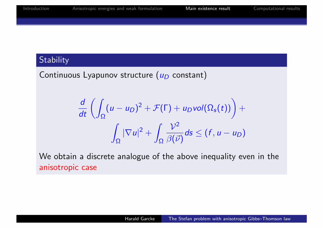
Stability
Continuous Lyapunov structure (uD constant)
d
dt
(∫Ω
(u − uD)2 + F(Γ) + uDvol(Ωs(t))
)+∫
Ω|∇u|2 +
∫Ω
V2
β(~ν)ds ≤ (f , u − uD)
We obtain a discrete analogue of the above inequality even in theanisotropic case
Harald Garcke The Stefan problem with anisotropic Gibbs–Thomson law

Introduction Anisotropic energies and weak formulation Main existence result Computational results
Mullins Sekerka instability in 2D
undercooling S = 1, isotropic surface energy 5× 10⁻³, 2× 10⁻³, 10−3
undercooling S = 1, cubic anisotropy with prefactor 5× 10⁻³, 2× 10⁻³, 10−3
Harald Garcke The Stefan problem with anisotropic Gibbs–Thomson law

Introduction Anisotropic energies and weak formulation Main existence result Computational results
Solidification with cubic anisotropy
Small sphere as initial data
Computation for different refinements. Oscillations disappearfor fine grids
Details of the evolution on finest gridHarald Garcke The Stefan problem with anisotropic Gibbs–Thomson law

Introduction Anisotropic energies and weak formulation Main existence result Computational results
Hexagonal symmetry (snow crystal symmetry)
Morphology
diagram of
Nakaya
2D-computationHarald Garcke The Stefan problem with anisotropic Gibbs–Thomson law
Introduction Anisotropic energies and weak formulation Main existence result Computational results
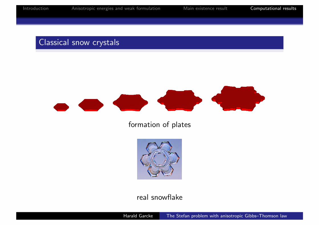
Classical snow crystals
formation of plates
real snowflake
Harald Garcke The Stefan problem with anisotropic Gibbs–Thomson law

Introduction Anisotropic energies and weak formulation Main existence result Computational results
Many forms need 3D computations
Formation of hollow columns (facet braking)
Compare analytical results by Giga and Rybka (2008)
real snowflakeHarald Garcke The Stefan problem with anisotropic Gibbs–Thomson law

Introduction Anisotropic energies and weak formulation Main existence result Computational results
Another 3D effect
A more pronounced real snowflake
Harald Garcke The Stefan problem with anisotropic Gibbs–Thomson law
Introduction Anisotropic energies and weak formulation Main existence result Computational results
Remarks and Conclusions
We showed global existence of weak solutions for the Stefanproblem with anisotropic Gibbs-Thomson law
The general crystalline case is still open
We introduced stable finite element discretization with goodmesh properties (No redistancing of mesh points necessary)
Hence: crystalline anisotropies can be approximated in astable and efficient way
The Stefan problem with anisotropic Gibbs-Thomson lawmodels realistic crystal growth phenomena
Harald Garcke The Stefan problem with anisotropic Gibbs–Thomson law