wireless channel modelling slides 4up

'

&

$

%School of ECS, Univ. of Southampton, UK. http://www-mobile.ecs.soton.ac.uk, c©L.-L. Yang 1/ 46

Wireless Channel Modeling

- An Overview -

Lie-Liang Yang

Communications Research GroupSchool of Electronics and Computer Science,

University of Southampton, SO17 1BJ, UK.Tel: +44 23 8059 3364, Fax: +44 23 8059 4508

Email: [email protected]

http://www-mobile.ecs.soton.ac.uk

'

&

$


Summary

Narrow-band wireless channels;

Propagation path-loss;

Shadowing slow fading;

Fast fading;

Power-budget design in wireless communications systems.

Wideband (frequency-selective) fading channels;

(Time-selective) fast fading channels;

Wideband (time-frequency-selective) fast fading channels;

Ultrawide bandwidth (UWB) channels.

'

&

$


Factors Affecting Wireless SignalTransmission

Propagation path-loss: The strength of radio wave decreases as the distancebetween the transmitter and receiver increases;

Reflection: When a radio wave propagating in one medium impinges uponanother medium having different electrical properties, the wave is partiallyreflected and partially transmitted;

Diffraction : Radio wave bends when it passes around an edge or through aslit. This bending is called diffraction;

Scattering: When a radio wave impinges on a rough surface, the reflectedenergy is spread out (diffused) in all directions due to scattering;

Doppler effect: When radio wave travels between two objects, the wavelengthchanges if one or both of them are moving. The Doppler effect is observedwhenever the source of waves is moving with respect to an observer.

'

&

$


Propagation Path-Loss - Free SpacePropagation

The free space propagation model is usually used to predictreceived signal strength, when the transmitter and receiver havea clear, unobstructed line-of-sight (LoS) path between them.

In free-space propagation environments the received signalpower decays with the square of the propagation path length,and the received signal power can be expressed as

Pr(d) = 10 log10

[

PtGT GR

(

λ

4πd

)2]

dBm (dBW) (1)

where Pt, Pr(d): transmitted and received power, GT , GR:antenna gains, d: distance between the transmitter and receiver,and λ: wavelength of the radio signal.

'

&

$


Shadowing Slow Fading

Figure 1: Illustration of the shadowing phenomenon.

'

&

$


Shadowing Slow Fading - Continued

Shadowing slow fading is mainly caused by terrain andtopographical features in the vicinity of the mobile receiver, suchas small hills and tall buildings;

In slow-fading analysis, the effects of both fast-fading andpath-loss must be removed;

Local-mean: The fast fading is removed by deriving the so-calledlocal-mean, which is obtained by averaging the signal level overa distance of typically some 20 wavelengths.

'

&

$


Shadowing Slow Fading - Continued

Based on empirical measurements, it has been shown that thelocal mean follows a lognormal distribution;

Let Ωt represents the local-mean. Then, Ωt obeys the lognormaldistribution having the PDF given by

pΩt(r) =

ξ√2πσΩt

rexp

[

−(10 log10 r − µΩt)2

2σ2Ωt

]

, r > 0 (2)

where

ξ = 10/ ln 10 = 4.3429;

µΩt(dB) and σΩt

(dB) are the mean and standard deviation of10 log10 Ωt, σΩt

ranges from 5 dB to 12 dB.

'

&

$


Lognormal distributed PDF

0 1 2 3 4 5 6 7 8Local Mean, t

0.0

0.2

0.4

0.6

0.8

PDF

t=0 dB,

2t=8 dB

Figure 2: Lognormal distributed PDF seen in (2).

'

&

$


Fast Fading

Fast fading is also referred to as small-scale fading, which accountsfor the rapid variation of signal levels, when the user terminal moveswithin a small or local area. There are many physical factors in theradio propagation channel, which result in fast fading, whichtypically include

Multipath propagation;

Doppler effect;

Carrier-frequency, bandwidth and symbol rate of the transmittedsignal, etc.

'

&

$


BS

MS

Figure 3: Illustration of multipath propagation of radio signals, where the receivedsignal at the MS consists of N multipath signals generated by the reflecting objectsaround the mobile terminal.

'

&

$


Narrowband - Fast Fading Consider the transmission of a narrowband signal, which is

expressed as

s(t) = <s(t) exp (j2πfct) (3)

where <x denotes the real part of x, s(t) is the complexbaseband signal depending on the specific baseband modu-lation scheme employed, fc represents the carrier-frequency.

Due to multipath propagations and Doppler frequency shifts,the received signal can be expressed as

r(t) =N∑

n=1

<y(t) exp (j2πfct) + n(t) (4)

where n(t) denotes the AWGN.

'

&

$


Fast Fading - Continued

In (4) y(t) can be expressed as

y(t) =N∑

n=1

αn(t) exp (−jϕn(t)) s(t − τn(t)) (5)

= yI(t) − jyQ(t) (6)

where

ϕn(t) = −φn(t) + 2π [(fc + fDn(t)) τn(t) − fDn(t)t] (7)

Hence, the received signal consists of a series of attenuated,time-delayed, phase shifted replicas of the transmitted signal.

'

&

$


r(t)=r1(t)+r2(t)+r3(t)+r4(t)

r1(t), r2(t), r3(t), r4(t)

0.0 0.5 1.0 1.5 2.0 2.5 3.0time, t

-4

-2

0

2

4

Am

plitu

de,A

(t)

Figure 4: Illustration of constructive and destructive effects of multipath signals.

'

&

$


Fast Fading - Important Concepts

Maximum delay spread, Tm;

Maximum Doppler frequency shift, fD;

Coherence bandwidth of a wireless channel, (∆f)c ≈ 1/Tm;

Coherence time of a wireless channel, (∆t)c ≈ 1/(2fD)

'

&

$


Fast Fading - Envelope and PhaseDistribution

The envelope and phase of a wireless channel are given by

α(t) =√

y2I (t) + y2

Q(t) (8)

θ(t) = − tan−1

[

yQ(t)

yI(t)

]

(9)

'

&

$


Correlated Rayleigh-distributed envelope

0 100 200 300 400

Time-40

-30

-20

-10

0

10

Env

elop

e(d

B)

Figure 5: Envelope distributions of a Rayleigh fading channel, when assumingthat the normalized Doppler frequency shift is fDT = 0.1, where T represents thesampling spacing.

'

&

$


Phase distribution of correlated fading channels

0 100 200 300 400

Time-4

-3

-2

-1

0

1

2

3

4

Phas

e

Figure 6: Phase distributions of a Rayleigh fading channel, when assuming thatthe normalized Doppler frequency shift is fDT = 0.1.

'

&

$


Fast Fading - Rayleigh Fading

Rayleigh fading channels belong to a class of channels,where the received envelopes of faded signals obey Rayleighdistribution;

Rayleigh distribution is commonly employed for describingthe statistical time varying nature of the received envelope inisotropic scattering environments, where exists no LoS prop-agation path between the transmitter and the receiver;

The Rayleigh PDF is given by

pα(t)(y) =2y

Ωexp

(

−y2

Ω

)

, y ≥ 0 (10)

where Ω = E[α2(t)].

'

&

$


0 1 2 3 4Amplitude, y

0.0

0.2

0.4

0.6

0.8

1.0

PDF

Figure 7: Illustration of the Rayleigh distributed PDF associated with Ω = 1.

'

&

$


Fast Fading - Rician Fading Rician distribution is commonly used for describing the statistical time

varying nature of the received envelope, when a signal is transmitted overan environment, where, in addition to many reflecting objects around thereceiver, exists a LoS propagation route between the transmitter and thereceiver;

It can also be used for describing the envelope distribution of the receivedsignal, when it contains a dominant non-faded component, although thisdominant component is not the LoS one;

The Rician PDF is given by

pα(t)(y) =2(K + 1)y

Ωexp

[

−K − (K + 1)y2

Ω

]

I0

(

2y

√

K(K + 1)

Ω

)

(11)

where K represents the ratio of the power in the specular component andthat in the scattering components of the received signal.

'

&

$


K=50

K=10K=5K=1K=0

0 1 2 3Amplitude, y

0

1

2

3

4

PDF

Figure 8: Illustration of the Rician distributed PDF of (11) associated with Ω = 1.

'

&

$


Fast Fading - Nakagami Fading

Nakagami-m distribution is a generalized distribution, whichoften gives the best fit to land-mobile and indoor-mobile mul-tipath propagation environments;

A good fit to these widely varying propagation scenarios isachieved by varying single parameter of m in the Nakagami-m distribution;

Nakagami-m distribution offers features of analytical conve-nience, which makes it possible to evaluate wireless sys-tem’s performance by using both analytical and numerical ap-proaches.

'

&

$


Fast Fading - Nakagami Fading (Continued)

The Nakagami-m distribution is given by

pα(t)(y) =2

Γ(m)

(m

Ω

)m

y2m−1 exp

(−my2

Ω

)

, y ≥ 0 (12)

where Γ(·) is the gamma function;

m = 1: Rayleigh fading;

m → ∞: Gaussian PDF;

m = 1/2: one-side Gaussian fading, the worst fading con-dition;

The Rician and lognormal distributions can also be closelyapproximated by the Nakagami distribution in conjunctionwith m > 1 values.

'

&

$


m=10m=5m=2m=1.5m=1m=0.5

0 1 2 3Amplitude, y

0

1

2

3

PDF

Figure 9: Illustration of the Nakagami-m distributed PDF associated with Ω = 1.

'

&

$


Power-Budget Design

Factors affecting the power-budget design:

Propagation path-loss;

Shadowing slow fading;

Fast fading.

'

&

$


power-loss due to slow

Slow fading margin or

Fast fading margin or

power-loss due to fast

Path-loss

Power-loss due to path-loss

Mobile terminal

0 d

DistanceBase station

fading, Lfast (dB)

fading, Lslow (dB)

PL(d) (dB)

Power (dBm)

Outage probability 1% - 2%

Outage probability 1% - 2%

Transmitted power required, PTx(dBm)

Minimum received power required, PRx(dBm)

Figure 10: Power-budget design for mobile systems, where the transmitted powermust satisfy PTx

≥ RRx+ Lfast + Lslow + PL(d)

'

&

$


Wideband (Frequency-Selective) FadingChannels

For narrowband signal, the signal bandwidth, say Ws, is sufficiently smallin comparison with the coherence bandwidth (∆f)c = 1/Tm of the corre-sponding wireless channel, i.e., Ws/(∆f)c = WsTm << 1;

Narrowband channel belongs to flat fading channels, where all the fre-quency components of the transmitted signal behave similarly;

For wideband signal, the signal bandwidth, Ws, may be significantly higherthan the coherence bandwidth (∆f)c = 1/Tm of the corresponding wire-less channel, i.e., Ws/(∆f)c = WsTm >> 1;

Consequently, two frequency components separated by a frequency ofthe coherence bandwidth or beyond may behave significantly differently;

Hence, wideband channels are typically frequency-selective fading chan-nels.

'

&

$


Envelope Correlation as A Function ofFrequency Separation

Assume Nakagami fading channels. Then, when the excessdelay-spread obeys the exponential distribution, it can be shownthat the correlation coefficient as a function of the frequency sep-aration ∆f = fv − fu, for the envelopes at fu and fv, can beexpressed as

ρE(∆f) ≈ Γ2(

m + 12

)

4m[

mΓ2(m) − Γ2(

m + 12

)]

1

1 + σ2τ (2π∆f)2

(13)

where στ represents the mean value of the excess delay spread.

'

&

$


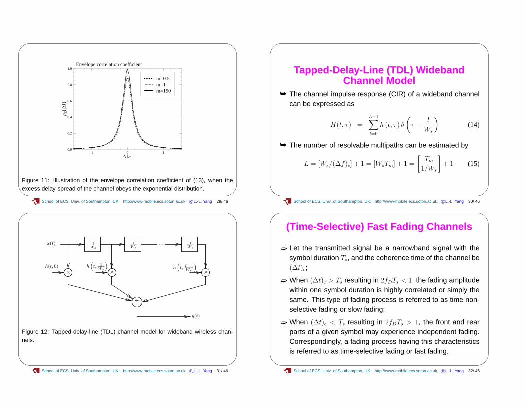
Envelope correlation coefficient

-1 0 1f

0.0

0.2

0.4

0.6

0.8

1.0E(

f)

m=150m=1m=0.5

Figure 11: Illustration of the envelope correlation coefficient of (13), when theexcess delay-spread of the channel obeys the exponential distribution.

'

&

$


Tapped-Delay-Line (TDL) WidebandChannel Model

The channel impulse response (CIR) of a wideband channelcan be expressed as

H(t, τ) =L−1∑

l=0

h (t, τ) δ

(

τ − l

Ws

)

(14)

The number of resolvable multipaths can be estimated by

L = [Ws/(∆f)c] + 1 = [WsTm] + 1 =

[

Tm

1/Ws

]

+ 1 (15)

'

&

$


y(t)

x(t)

h(t, 0)

×

+

××

1

Ws

1

Ws

1

Ws

h(

t, 1

Ws

)

h(

t, L−1

Ws

)

Figure 12: Tapped-delay-line (TDL) channel model for wideband wireless chan-nels.

'

&

$


(Time-Selective) Fast Fading Channels

Let the transmitted signal be a narrowband signal with thesymbol duration Ts, and the coherence time of the channel be(∆t)c;

When (∆t)c > Ts resulting in 2fDTs < 1, the fading amplitudewithin one symbol duration is highly correlated or simply thesame. This type of fading process is referred to as time non-selective fading or slow fading;

When (∆t)c < Ts resulting in 2fDTs > 1, the front and rearparts of a given symbol may experience independent fading.Correspondingly, a fading process having this characteristicsis referred to as time-selective fading or fast fading.

'

&

$


Envelope Correlation as A Function of TimeSeparation

Assuming a Nakagami fading channel, the envelope corre-lation coefficient ρE(∆t) with a time-spacing ∆t can be ex-pressed as

ρE(∆t) ≈ Γ2(

m + 12

)

ρ2∆t

4m[

mΓ2(m) − Γ2(

m + 12

)] (16)

where ρ∆t = J0(2πfD∆t).

'

&

$


Envelope correlation coefficient

-1 0 1fD t

0.0

0.2

0.4

0.6

0.8

1.0

E(

t)

m=150m=1m=0.5

Figure 13: Illustration of the envelope correlation coefficient of (16), when thechannel is assumed to be WSSUS.

'

&

$


Tapped-Frequency-Shift-Line (TFSL) FastFading Channel Model

For fast fading channel, the frequency-domain CIR can beexpressed as

Y (F ) =

(L−1)/2∑

l=−(L−1)/2

h (F, f) δ

(

f − l

Ts

)

(17)


L ≈[

Ts

1/2fD

]

+ 1 ≈ 2 [fDTs] + 1 = 2

[

fD

1/Ts

]

+ 1 (18)

'

&

$


h(

F,−L−1

2Ts

)

y(t)

+

1

Ts

1

Ts

1

Ts

X(

F + L−1

2Ts

)

X(

F − L−1

2Ts

)

h(

F, L−1

2Ts

)

h(

F,−L−1

2Ts+ 1

)

Figure 14: Tapped-frequency-shift-line (TFSL) channel model for time-selectivefading channels.

'

&

$


Wideband (Time-Frequency Selective) FastFading Channels

In practice, a wireless channel may simultaneously satisfy thefrequency-selective fading condition of WsTm > 1 and thetime-selective fading condition of 2fDTs > 1;

In this case, a signal transmitted over this type of wirelesschannels experiences both frequency-selective fading andtime-selective fading;

This type of channels is classified as time-frequency-selectivefading channels.

'

&

$


-20-15-10-505

Envelope Amplitude, (dB)

0 20 40 60 80 100 120Time Index 0 20 40 60 80 100 120

Frequency Index

−20

−15

−10

−5

0

5

Figure 15: Illustration of the time-frequency selectivity of a 10-path wireless chan-nel associated with the normalized Doppler frequency spread of fDT = 0.02.

'

&

$


Envelope Correlation as A Function ofTime-Frequency Separations

Assuming Nakagami fading channels and that the excessdelay-spread obey the exponential distribution with the pa-rameter of στ , then, the envelope correlation coefficient as afunction of ∆f and ∆t can be expressed as

ρE(∆f, ∆t) ≈ Γ2(

m + 12

)

4m[

mΓ2(m) − Γ2(

m + 12

)]

J20 (2πfD∆t)

1 + σ2τ (2π∆f)2

(19)

'

&

$


00.20.40.60.81

ρE

(∆f,∆

t)

−2−1.5 −1−0.5 0 0.5 1 1.5 2fD∆t − 2− 1.5− 1− 0.5 0 0.5 1 1.5 2

∆fστ

0

0.2

0.4

0.6

0.8

1

Figure 16: Illustration of the envelope correlation coefficient of wireless channels.

'

&

$


Two-Dimensional (2-D) Channel Model forTime-Frequency Selective Fading

Channels. For wideband time-frequency-selective fast fading channels,

the CIR can modeled as

H(t, f, τ) =M−1∑

m=0

L−1∑

l=0

h (t, f, τ) δ

(

τ − l

Ws

)

δ

(

f − m

Ts

)

(20)


ML ≈([

Ws

1/Tm

]

+ 1

)([

Ts

1/2fD

]

+ 1

)

= ([WsTm] + 1) (2 [fDTs] + 1) (21)

'

&

$


............

............

............

............

............

............

h00 h01

×

+

1/Ws 1/Ws 1/Ws

×

+

××

1/Ws 1/Ws 1/Ws

×

+

××

1/Ws 1/Ws 1/Ws

1/Ts

−1/Ts

+y(t)

x(t)

× ×h−10 h

−11

h10 h11

h−1(L−1)

h0(L−1)

h1(L−1)

'

&

$


Ultrawide Bandwidth (UWB) Systems -Characteristics

UWB characterizes transmission systems with instantaneous spectral oc-cupancy in excess of 500 MHz, or a fractional bandwidth of more than20%;

Currently, UWB is mainly recommended for short-range (such as in-door and sensor networks), high-speed (which may be upto hundreds ofMbits/s) multiple-access communications;

High processing gain and low power spectral density;

Fine delay resolution probably resulting in a huge number of multipathcomponents;

Accurate position location and ranging;

Property of material penetration due to low frequency components.

'

&

$


UWB Indoor Channel Modeling

The measurements in UWB channels show that the envelopeamplitudes do not follow a Rayleigh distribution. Either log-normal or Nakagami distribution can equally be used for fittingthe measurement data;

Multipath components arrive at the receiver in group (clus-ters). Cluster arrival time obeys Poisson distribution;

The arrival time of the multipath components within a clusteralso obeys Poisson distribution;

'

&

$


Multipath UWB Indoor Channel Model (IEEE802.15.3a)

Let the cluster arrival rate be Λ, and the arrival rate of the multipaths withina cluster be λ. Usually, we have λ > Λ.

The channel impulse response (CIR) of the multipath UWB channel isrecommended as

h(t) =

M−1∑

m=0

L−1∑

l=0

hmlδ(t − Tm − τml) (22)

where

Tm + τml denotes the arrival time of the lth multipath component of themth cluster;

hml = |hml| exp(jθml) is the channel gain of lth multipath componentof the mth cluster;

M is the number of clusters, while L is the number of multipath com-ponents within a cluster.

'

&

$


Multipath UWB Indoor Channel Model (IEEE802.15.3a) - Continued

The multipath amplitude |hml| can be modeled by lognormalor Nakagami distribution, with the power given by

E[|hml|2] = E[|h00|2] exp

(

−Tm

Γ− τml

γ

)

, Γ > γ (23)

The distributions of the cluster arrival time and the multipath(within a cluster) arrival time are given by

p(Tm|Tm−1) = Λ exp[−Λ(Tm − Tm−1)], m > 0 (24)

p(τml|τml−1) = λ exp[−λ(τml − τm(l−1))], l > 0 (25)

wireless channel modelling slides 4up

Documents

school of ecs

radio signal

strength of radio wave

university of southampton

radio wave travels

radio wave propagating

radio wave bends

shadowing slow fadingfigure