Winglet Effect on Induced Drag for a Cessna 172 Wing

Alexander Schumacher Erik Sjögren

Tobias Persson

Bachelor Thesis 2014-05-18

KTH Flygteknik

Farkost och flyg

SE-100 44 STOCKHOLM

2

ABSTRACT

The perfect wing is a dream that many airplane manufactures have been striving to achieve since

the beginning of the airplane. The goals are usually the same for everyone;

Increase lift

Reduce drag

Minimize weight

A combination of these goals lead to a decrease in fuel consumption, which in turn reduces

pollution in our atmosphere with the added bonus of an increase in economic revenue.

One way to improve performance is to modify the tip of the wing structure, which has become a

common sight on today’s airplanes. With the help of computational programs, the effects on drag

due to wingtip devices can be previewed.

3

NOMENCLATURE

V Free stream speed

α Angle of attack

αe Effective angle of attack

αi Induced angle of attack

CDi Induced coefficient of drag

L Lift force

ρ Density

S Wing reference area

e Efficiency factor

AR Aspect Ratio

b Wingspan

c Chord length

m Mass

T Thrust Force

g Constant of gravity

D Drag Force

CL Coefficient of Lift

Di Induced Drag Force

q Dynamic pressure

4

TABLE OF CONTENTS

ABSTRACT 2

NOMENCLATURE 3

TABLE OF CONTENTS 4

1 INTRODUCTION 6

1.1 Background 6

1.2 Purpose 6

1.3 Delimitations 6

1.4 Method 7

2 THEORY 8

2.1 Wingtip Design 8

2.2 Induced Drag and Minimum Induced Drag 9

2.2.1 Induced Drag 9

2.2.2 Minimum Induced Drag 10

2.3 Twist Distribution 10

2.4 Vortex Lattice Method 12

2.5 Steady Level Flight 13

3 RESTRICTIONS 15

3.1 Airplane Modeling 15

3.2 Infinite Winglet Designs 15

3.3 Flight State 15

4 METHOD 16

4.1 Analysis of a wing in XFLR5 16

4.1.1 Modeling of the Cessna Wing 16

4.1.2 Airfoil Analysis 17

5

4.1.3 Wing Analysis 18

4.1.4 Results from the Analysis 20

4.2 Calculating and Comparing Winglets 20

4.2.1 Main Concept 20

4.2.2 Wing Data and Comparison 22

5 RESULTS 26

6 DISCUSSION AND CONCLUSIONS 32

6.1 Discussion 32

6.1.1 Project History 32

6.1.2 Result Discussion 33

6.1.3 Alternative Tests 35

6.2 Conclusions 36

6.3 Division of Labor 36

7 REFERENCES 37

6

1 INTRODUCTION

1.1 Background

Winglets are widely used on larger commercial and military aircrafts to reduce fuel consumption

by minimizing drag and maintaining or increasing lift. These winglets are usually not as common

on smaller aircrafts that are found in general aviation. Here a question arose as to how much do

winglets affect an aircraft, and what aeronautical effects result from these winglets? What

happens to the induced drag caused by the winglets? Do the resulting structural loads on the

wing vary drastically? Can these winglets be applied to the wings of a general aviation aircraft

and will it be beneficial?

Since its start in 1955, more Cessna 172s have been built than any other aircraft [1]. The classic,

almost rectangular, wing is easy to spot with it resting on the canopy of its body. The Cessna

172’s popularity makes it a great candidate to use as a reference wing for winglet testing within

general aviation.

XFLR5 is a well-used platform amongst hobby builders and airplane architects that want to

experiment on new or old wing designs. The program is a tool that that lets users program wing

designs and analysis based on the Lifting Line Theory, Vortex Lattice Method, and on 3-D Panel

Method. Here a user can define a wing at a series of angles of attack, at different speeds, and

with varying conditions. XFLR5 gives the user the opportunity to make their own wing and put it

through thousands of tests. Everything from a 2-D airfoil to a 3-D CAD of the wing can be done

in XFLR5.

In the following chapters the wing of a Cessna 172 will undergo several winglet modifications

and be tested to see what effects they have on a wing. These modifications can be done thanks to

XFLR5 with a goal to decrease the drag without creating too much structural load on the aircraft.

Several key factors include the flight conditions, twist distribution, the design of the winglets,

and the net forces resulting from the above modifications.

1.2 Purpose

With the help of XFLR5 a replica Cessna 172 wing will be modeled and wingtips will be applied

to the existing wing to see what effects these cause on the aerodynamics of the wing. The wing

lengths and wingtip designs will vary. A comparison of these winglets will help the reader gain

an insight on winglets and their effects on the induced and total drags without increasing

structural loads at a steady-state flight.

The following chapters will inform the reader about XFLR5, how to orientate oneself in the

program, and how to retrieve data on a custom designed wing. XFLR5 reduces the need to build

a physical model of a wing or plane, making it a cheap and quick way to retrieve data that may

be vital for a plane to fly effectively.

1.3 Delimitations

The contents of the report are strictly focused on the aerodynamics of the wing of a Cessna 172

and what effects modifications of the wing have on the resulting data. The physics of the airplane

will not be discussed passed the point of a general discussion. The data that is generated will be

used to look at the induced and total drags created by different winglets on a Cessna 172 wing at

steady-state flight. The bending moment along the root of the wing will be discussed as well.

7

The program XFLR5 will be used to the extent that only a main wing will be analyzed instead of

the whole body of a plane or rear tail wing. The defining analysis will be constructed with a

varying angle of attack and a constant speed. Plane inertia is used along with the option of

viscosity. Several airplane and flight conditions will remain constant throughout the project.

1.4 Method

There are many factors that need to be taken into consideration in order to analyze the

aeronautical effects that wingtips have on a set wing. With the decision to use a Cessna 172 wing

it is essential that the original wing can be designed and programmed in XFLR5. A detailed

description of the main structures of a Cessna 172 wing can be found in Jane’s All the World’s

Aircraft [2]. Some key features include a NACA 2412 airfoil, root and tip chords, dihedral

angles, and incidence angles. These features are later implemented in XFLR5 to build the wing.

Once the wing is built, tests can be run at a constant velocity and varying angles of attack to see

how the wing behaves in flight. The vortex lattice method is applied across the wing to help

compute lift and induced drag at different parts of the wing. These results are used as a reference

to compare the effects of adding wingtips to the original wing.

To understand the properties of winglets on a wing, one form of winglet is chosen. There are

several variables that can be changed on this winglet design. The dihedral angle of the winglet,

the length of the wing/winglet, and the twist distribution along the wing are a few key factors of

the winglet design. Most of these factors will be tested and compared against each other and

ultimately compared to the original Cessna 172 wing that is used today.

In order to compare the results of every new wing, the induced drag and total drag are exported

from XFLR5 to MATLAB. The exported values are later interpolated and/or plotted so that

graphs can be set up to help analyze the data.

8

2 THEORY

2.1 Wingtip Design

Wingtip designs have been debated and discussed since the early 20th

century. There are nearly

an infinite amount of varying styles for winglets and other wingtip devices that have previously

been tested; some of these can be seen in Figure 2.1:

Figure 2.1. Different wingtip styles [3]

The true benefits of winglets have yet to be fully understood. There are many misconceptions

about how a winglet works, and what it actually does. Winglets are used to reduce trailing vortex

turbulence behind the wing, customize the lift distribution along the wing, and to increase the

aspect ratio without having to increase the wingspan. The former being the idea that winglets can

reduce the amount of induced drag from the wings. This is hard to achieve without increasing

weight, or profile drag due to an increase in wetted area and junction flows. There are a few

common misunderstandings about winglets that are important to discuss. The two most common

misconceptions can be read in D. McLean’s paper: Wingtip Devices: What They Do and How

They Do It [3]:

The “compactness myth”- the idea that the cores that contain all of the vorticity in the

vortex wake after rollup are very compact.

The “induction myth”- the trailing vortex sheet and the rolled-up vortex cores are the

direct cause of the vorticities everywhere else in the flow field and of induced drag.

The combination of the two points above gives an idea that induced drag is caused by the vortex

wake and that by making a local change to the flow in the core of a “tip vortex” will have a large

effect on the induced drag. This is extremely misleading.

Even with the help of mathematical theories, it is hard to design a bettered winglet. There are no

easy equations that give a detailed view of how the drag is affected by the varying modifications

of the winglets or the lift distribution. Although, the Trefftz-plane theory does explain that a

vertical winglet is most effective at reducing induced drag at the tip of the wing [3]. Through

testing several different samples of winglets, Cone was able to decipher that “any non-planar

shape that adds vertical height near the tip could reduce drag” [3].

Important to note is that a reduction in induced drag does not guarantee a net drag benefit. An

increase in parasitic drag due to addition of wetted area and junction flows may negatively affect

the total drag of the new wing. The attachment of wingtips will most likely increase the bending

9

moments on the entire wing resulting in a remodeling of the wing structure. This may cause a

greater total weight for the airplane, which will affect the flying benefits negatively.

Another factor that helps the effectiveness of the wing with an attached winglet is the twist

distribution. Attaching a winglet to an already optimized wing with a specific twist will most

likely not contribute to the net benefit. This means that attaching a winglet to the wing may mean

that a new twist distribution along the wing must be designed in order to optimize the new wing.

An important theme to keep in mind for winglet design is Whitcomb’s rule of thumb; “keep the

additional profile drag to a minimum through good aerodynamic design practice” [3], and “for a

given increase in bending moment, a near-vertical winglet offers nearly twice as much drag

reduction as a horizontal span extension.” [3]. Important to note is that, many other studies such

as, R.T. Jones’ 1980 paper, show that with a fixed structural weight, the induced drag reduction

is relatively the same.

2.2 Induced drag and minimum induced drag

2.2.1 Induced drag

The basic principle of generating lift on a wing is to achieve a lower pressure on the upper

surface of the wing compared to the lower. Consequently, a global flow pattern is obtained

which is shown in Figure 2.2.

Figure 2.2. Global flow pattern [3]

When producing lift on a wing, the air from the underside of the wing will move outwards from

the root and around the wing tip to meet the lower pressure flow. This reduces the pressure

difference and is known as the span-wise pressure gradient. The effects of the pressure gradient

decreases towards the wing root. As viewed from the front or rear of the aircraft the upward flow

at the wingtips seems to produce vortices, also called trailing vortices. The vortices around the

wing change the upstream airflow near the wing and deflects the flow down, also known as

downwash. This leads to a decrease in the effective angle of attack due to the upstream flow near

the wing being deflected down. The decrease in the effective angle of attack leads to a reduction

in the lift force on the wing. Since all of the input energy for flight that does not contribute to the

lift on the wing can be considered as drag, the loss of lift is felt as an extra drag, which is known

as lift induced drag (a consequence of generated lift). An illustration of the induced drag is

10

shown in Figure 2.3, where V is the free stream direction, α is the angle of attack, αe the effective

angle of attack and αi the induced angle of attack.

Figure 2.3. Illustration of induced drag.

The induced drag coefficient can be expressed as:

2

2 4 21

4

Di

LC

V S eAR

, (2.1)

where L is the lift force, ρ is the free stream density, S is the wing reference area, e is the wing

span efficiency factor by which the induced drag exceeds that of an elliptical distribution and AR

is the aspect ratio. The aspect ratio is defined by

2b

ARS

, (2.2)

where b is the total wingspan. As one can observe, the induced drag is proportional to the lift

force squared and inversely proportional to the aspect ratio.

2.2.2 Minimum induced drag

It can be shown that for a given wingspan and lift, minimum induced drag is produced when the

span-wise lift distribution is elliptical [4]. This is valid for a planar wing. For a wing where the

planar wing assumption is not accurate, the elliptic span-wise lift distribution may not be

optimal.

2.3 Twist Distribution

By applying a lateral twist on a planar wing, one can begin to change the span-wise distribution

of lift. By “twisting” the wing, the local angle of attack is changed resulting in a change on the

local lift coefficients. On a “flat” wing, an elliptical distribution is optimum [4]. The difference

in wing shapes lead to different wing twist distributions. It is important to note that in order to

avoid stalling, the wing must be designed so that the stall begins as close to the wing root as

possible [5]. A few examples of wing styles can be seen in Figure 2.4 below:

11

Figure 2.4. Three examples of planar wings [6]

From Arne Karlsson’s notes on elliptic load distribution [5], a planar wing with an elliptic load

distribution is represented from the following equation,

2

2

21L

g i

C bc

AR

, (2.3)

where

Li

C

AR

. (2.4)

Here, g is the geometric angle of attack and i is the induced angle of attack. is the

dimensionless lateral coordinate along the wing, with 0 at the wing root, and 1 at the wing tip. c

is the chord length and b the wing span.

For a thin section of the airfoil the local lift coefficient is used:

2 2l eff g ic . (2.5)

The effective angle of attack, eff, is measured from the zero-lift line of the airfoil section.

An elliptical wing, also known as a Spitfire wing, is already designed to have an elliptical

distribution, meaning that there is no twist needed. For a rectangular wing with a constant chord,

c, the twist distribution can be described by the following equation:

2

0 1g i , (2.6)

where

0 2

2 LC

. (2.7)

The local lift coefficient at a lateral position along the wing is later found:

2

02 1lc . (2.8)

In the case of the Cessna 172, the wing is neither elliptical or rectangular. The wing is symmetric

along the root chord, meaning that,

12

cl () = cl (-). (2.9)

From Equation (2.3) the lateral distribution of the geometric angle of attack is found:

2

2

21L

g i

C b

ARc

. (2.10)

The span-wise distribution of cl is found by combining the above equation with Equation (2.6):

24

1l

L

c b

C ARc

. (2.11)

The above equations are set towards finding an elliptic distribution along a planar wing, but

when winglets are added the wing is no longer “flat.” Here an elliptic distribution is not

necessarily the most effective distribution for the wing. [3] These “ideal” distributions for a wing

with winglets are different depending on how the wing will be used. The loads may be

distributed depending on bending loads, and other factors such as engine position, fuselage, wing

weight, etc.

2.4 Vortex lattice method

Analysis of a 3-D wing can be performed in XFLR5 using the Vortice Lattice Method (VLM).

This method models the wing as a set of panels, all associated with a single horseshoe vortex. A

horseshoe vortex consists of one vortex in the span-wise direction of the wing and two trailing

vortices directed opposite the direction of flight, see Figure 2.4.

Figure 2.4. Horseshoe vortices defined for each panel of the wing [7]

As boundary conditions, the so-called no slip condition is used, which states that the velocity

normal to the surface must be zero. The velocity on a panel depends on the free stream velocity

but also on the velocity induced by the vortices on each of the panels. This gives a linear

equation system from were the unknown vortex strengths can be solved.

13

When the circulation for each panel segment is known, the lift of a specific panel can be

calculated with the Kutta-Joukowski theorem. Finally, the total lift of the wing is obtained by

summating the lift contribution from all the panels.

In the classic vortex lattice method inviscid flow is considered. The XFLR5 implementation is

however modified to take viscous effects into account. [7]

2.5 Steady Level Flight

Steady level flight is the point at which an aircraft is cruising at a constant speed. When flying at

a constant speed, the airplane is in a state of inertia where all the acting forces on the airplane are

in equilibrium. The general forces acting on the plane are seen in Figure 1 bellow,

Figure 2.5. Free diagram of forces on a Cessna 172

Where T represents the thrust produced by the aerodynamic force R. The drag is defined as D in

the figure above, as well as L represents the lift. In the free diagram, mg represents the force

created by gravitational acceleration and the mass of the plane. The angle between the trust and

velocity vectors is defined as . In a steady level flight there is no acceleration. As a result, all

the forces must be balanced.

: sin 0L T mg (2.12)

: cos 0L D (2.13)

The angle between thrust and the speed vectors is usually small and for the following

calculations

0 . From above, the following must be true:

L mg , (2.14)

and

T D . (2.15)

With the mass of the plane defined and the gravitational acceleration known, L can be defined. L

is often assumed constant as long as mg does not change.

Important to note is the CL that is calculated for the steady state flight does not exceed the

maximum CL where the wing will result in a stall. In order to find the CL, the following equation

can be used,

14

21

2

L

LC

V S

, (2.16)

where is the surrounding atmosphere density, V is the speed of the airplane, and S is the

reference area of the wing. The calculated CL for steady level flight must be less than the CL at

which the wing results in a stall. [8]

15

3 RESTRICTIONS

In order to compare the results from the modified wings, it is necessary to set up certain

restrictions or definitions. These restrictions/definitions involve defining specific airplane

designs, flight states, and winglet designs.

3.1 Airplane Modeling

To understand how the drag is affected along the varying wings, the body and tail wing of the

Cessna 172 are ignored. The following procedures and results in this report are limited to strictly

looking at the main wing. Here the values have been taken from Jane’s All the World’s Aircraft

[3] for the original wing. For this project, it is inferred that all the lift on the airplane is done

from this wing. Parts, such as the fuselage and wing flaps are not taken into consideration. Fluid

effects from the propeller are also ignored.

Other airplane features that are disregarded are wing size, length, and weight. When looking to

build a real wing, all three of these features should be analyzed. In this project, aspects such as

typical garage heights and FAA limitations of wing lengths are not necessary when

understanding the effects of wing designs on drag. Weight will have an impact on bending

moments along the wing, as well as an increase in engine power or fuel consumption, although

for this study effects on the plane due to weight are overlooked. The main focus is to look at how

drag on the Cessna 172 wing changes due to different winglet designs, here the above three

factors do not have a direct effect on the project.

The root bending moment constraint for all the wings in this project will be defined by the results

for bending moment from the original twisted Cessna 172 wing in XFLR5. The root bending

moments for the varying wings with winglets may not exceed this maximum by more than 0.5%.

3.2 Infinite Winglet Designs

There are an infinite amount of different winglet designs that can be applied to wings. Winglet

size, twist, airfoil, design, and position are just a few parameters that need to be decided before

beginning to compare effects on the induced drag. As for this study; the dihedral angles, winglet

chords, winglet airfoils, and winglet positioning have been discussed and defined.

The resources and time allotted are not sufficient to consistently test the infinite different winglet

configurations. The above restrictions, may not give the optimum winglet for the Cessna 172, but

should be sufficient enough to see the effects that winglets do have on the wing.

3.3 Flight State

An airplane undergoes several flight positions once in flight. The behavior of the wing changes

as the plane flies at different altitudes, speeds, climbs or descents, etc. In order to establish

consistency, the plane is set at a steady level flight at a defined altitude with a constant speed and

density. As seen in Equation (2.14), a desired lift force is defined and used. The winglets may

affect the drag and lift differently at varying speeds or angles of attack, but as for this report the

wing will strictly remain at a steady level flight.

16

4 METHOD

4.1 Analysis of a wing in XFLR5

4.1.1 Modeling of the Cessna wing

The following chapter describes how XFLR5 can be used for a wing analysis, more specifically,

how an analysis can be performed on the wing of the Cessna 172. The program can produce a

variety of data, including: the lift, drag, span-wise load distribution, and bending moment along

the wing. Dimensions used to model the wing are taken from Jane’s All the World’s Aircraft [3]

and can be seen in Table 4.1 below. The chord is defined as constant from the root to the middle

section of the wing, this can be seen in Figure 4.1. Thereafter, the chord is linearly distributed to

the tip. The used chord distribution is seen in Figure 4.2.

Cessna 172 Data

Airfoil NACA 2412

Wing Span 11 m

Root Chord 1.63 m

Tip Chord 1.13 m

Dihedral 1.7 °

Twist at root 1.5 °

Twist at tip -1.5 °

AR (Aspect Ratio) 7.5

Table 4.1. Data for the Cessna 172 from Jane’s All the World’s Aircraft [3]

Figure 4.1. Top view of Cessna 172 [9]

17

Figure 4.2. Estimated Distribution of Chord Length

In order to compare the different wings, the flight conditions must be specified. The chosen data

representing a typical flight can be seen in Table 4.2 below. The values used for the speed and

weight of the plane are taken from Jane’s All the World’s Aircraft [3]. The flying altitude is set

to 2000 m. The remaining parameters are taken from the US Standard Atmosphere [10] and

correspond to the chosen altitude.

Flight Data

Cruising speed, Cessna 172R 80% power 63 m/s

Max T-O weight, Cessna 172R 1111 kg

Altitude 2000 m

Mach Number 0.19

Air Density 1.007 kg/m3

Air Viscosity 1.714∙10-5

m2/s

Acceleration of Gravity 9.80 m2/s

Table 4.2. Flight data used for the analysis

4.1.2 Airfoil analysis

The analysis of a wing in XFLR5 starts with the definition of an airfoil, which is done in the

mode “Foil Direct Design”. For this project the NACA 2412 airfoil of the Cessna wing is used.

An analysis using a number of different conditions can be performed on the created airfoil. The

analyzed data for a given condition is referred to as a polar and can be tested under the mode

“Direct Foil Analysis”.

In this project, a “Type 1” analysis is used for the polars, where the velocity is held constant and

the flight data is calculated at different angles of attack. For the analysis, Reynolds number and

the Mach number must be specified. The 3-D model of the wing is essentially built up from 2-D

airfoils with varying chord lengths, meaning that the Reynolds number will vary along the span

of the wing. Therefore, the range of Reynolds numbers used for the analysis should be decided

according to the chord length of the wing. In a “Batch Foil Analysis” (Figure 3), the program

allows the user to specify a range of Reynolds numbers where one can calculate the polars.

-1 -0.8 -0.6 -0.4 -0.2 0 0.2 0.4 0.6 0.8 11.1

1.2

1.3

1.4

1.5

1.6

1.7

1.8Chord Length vs Span

Lateral Coordinate

Chord

Length

[m

]

18

Fig 4.3. Analysis settings for a batch foil analysis in XFLR5

4.1.3 Wing analysis

With the generated polars, an analysis can be performed on the full 3-D wing in the “Wing and

Plane Design” mode. The wing is created by defining cross sections at different span-wise

positions along the wing. Each cross section is defined by its airfoil, chord length, dihedral angle,

twist angle, and leading edge offset.

To create a specific twist distribution for the wing one must define the twist at a number of extra

cross sections. In XFLR5, the twist distribution is linear between two cross sections. Extra cross

sections are used as a form of discretization in order to achieve the preferred twist. This is done

for the original Cessna 172 wing, where the desired twist distribution was decided from equation

(2.10). For this report, it is assumed that an elliptic lift distribution is desired for the original

wing. An important factor when twisting the wing is to make sure that the geometric angle of

attack at the root is greater than the g at the wing tips in order to avoid stalling during flight.

The CL corresponding to a steady level flight was used in equation (2.10). This CL can be decided

from equation (2.7) using L from equation (2.14). Figure 4.4 below shows how the different

cross sections of the wing are defined.

19

Figure 4.4: Defining a Wing With Different Cross Sections in XFLR5

XFLR5 offers different analysis methods, based on the lifting line theory (LLT), the vortex

lattice method (VLM), and a 3-D panel method. For a wing with high dihedral angles, as in the

case of winglets, the LLT is not recommended. The main use for the 3-D panel method is to take

the effects of the plane’s body into account. Since this project only focuses on the main wing,

there is no need to use this method. Instead the VLM is used as it is most suitable for a wing with

winglets.

Again, a “Type 1” analysis is performed in which the velocity is kept constant. Viscous effects

are ignored in the classic VLM, however, XFLR5 offers an option to include viscous effects.

These results are extrapolated from the 2-D model [11]. The viscous option is used in this

project. Free stream speed, air density and viscosity from Table 4.2 are used, as seen in Figure

4.5.

20

Figure 4.5. Settings for a wing analysis in XFLR5

4.1.4 Results from the analysis

After a completed analysis various data is returned to the user. In this project the lift, drag, and

bending moment are studied and compared at each individual new wing design. The results can

be studied in graphs directly in XFLR5, or exported to an Excel file, which is done in this

project. The data is then read in MATLAB and analyzed in more detail.

4.2 Calculating and Comparing Winglets

4.2.1 Main Concept

In this chapter, an attempt to compare the effects from different winglets on the induced drag and

total drag will be done. The flight state considered is the steady level flight, which has been

discussed in Theory. From Equation (2.14), the lift force needed is equal to the weight of the

plane (assumed to be constant for all winglets). The estimated mass of the plane and the

gravitational acceleration can be seen in Table 4.2. The lift force needed is

L mg 1111 9.80 10000 N . (4.1)

In order to have a thorough winglet comparison, as many parameters as possible are kept

constant. The remaining parameters are systematically altered. As a start, the original wing is

partitioned at 70 %, 80 % and 90 % of the total wingspan in the lateral direction. A visual

graphic of this is seen in Figure 4.6.

21

Figure 4.6. Sections of the original wing at 70 %, 80 % and 90 % of the wingspan

At each new section of the wing, wingtips of different lengths and dihedral angles are applied.

The same junction, see Figure 4.7, is used for all of the winglets tested. This junction is obtained

from a simple change in dihedral angle at the position where the winglet is applied. The airfoil is

the same for all of the winglets and is the same NACA 2412 airfoil that is used for the original

wing.

Figure 4.7. Junction of the winglets

Table 4.3 shows the systematic scheme of how the wingtips are designed.

Section Dihedral angle Wingtip length

70% 30 30

80

130

60 30

80

130

90 30

80

130

80% 30 30

22

80

130

60 30

80

130

90 30

80

130

90% 30 30

80

130

60 30

80

130

90 30

80

130

Table 4.3. Scheme of how variations of dihedral angles and wingtip lengths are made

4.2.2 Wing Data and Comparison

Without a moment constraint

A methodic overview of how to analyze the results from the varying winglets in Table 4.3 is

presented here.

The relation between the global induced drag coefficient and the global lift coefficient at a

discrete number of points is calculated with XFLR5. That is,

iD LC C , (4.2)

where CDi is the global induced drag coefficient. The induced drag coefficient can be defined as:

21

2

iDi

DC

V S

, (4.3)

where Di is the induced drag force.

The relation (4.2) can be modified to describe the forces related to the coefficients by

multiplying the coefficients with the dynamic pressure q, which is defined as:

21

2q V S . (4.4)

From equation (2.16) and equation (4.3) one can see that this leads to the relation:

[ ]iD L , (4.5)

23

where L is the lift force.

The discrete data points from XFLR5 are exported to MATLAB and interpolated to get the

induced drag at the desired lift more accurately. A second order interpolation polynomial is used,

as shown in Figure 6.

Figure 4.8 Interpolation of induced drag versus lift force

With a moment constraint

The winglet designs in Table 4.3 may not be optimal when trying to find the winglet effects at a

given root bending moment constraint, instead, a new comparison is done. If one wishes to be

able to compare different wings for a given airplane, in this case a Cessna 172, the root bending

moment obtained from the wings with winglets applied should be the same as for the original

wing. Some of the winglet configurations that follow from the scheme in Table 4.3 may exceed

the root bending moment constraint. To achieve a better comparison, the scheme in Table 4.3 is

modified so that for each dihedral angle, the wingtip length will be adjusted so the root bending

moment will be equal to the original wing. To clarify this, Table 4.4 shows the new scheme

followed here for one of the three sections.

Section Dihedral angle [°] Wingtip length [cm]

70 % 30 max

60 max

90 max

Table 4.4. Scheme of winglet designs to achieve the root bending moment constraint

Since the bending moment on a wing depends on the lift, it will vary with the angle of attack.

For each analyzed wing the angle of attack needed to maintain the steady level flight is

calculated. This is done by looking at the linear relation between the lift force and the angle of

attack. The data points calculated in XFLR5 are interpolated with a first degree polynomial as

shown in Figure 4.9.

0.2 0.4 0.6 0.8 1 1.2 1.4 1.6 1.8 2

x 104

0

100

200

300

400

500

600

700

800

900

Lift force [N]

Induced d

rag [

N]

Induced drag vs. lift

Interpolated 2nd degree polynomial

Data points

24

Figure 4.9 Interpolation of lift versus angle of attack

At the angle of attack that maintains the steady level flight, the bending moment distribution

along the wing is obtained from data calculated by XFLR5, see Figure 4.10.

Figure 4.10. Typical wing bending moment curve.

The root bending moment is obtained from Figure 4.10 at the horizontal point 0. The moment

distribution along the wing is related to a specific angle of attack and because the calculations in

XFLR5 are made for a discrete number of angles of attacks, the root bending moment can only

be obtained at these specified angles of attacks. To get a more accurate read of the root bending

moment at the desired angle of attack, the root bending moment at different angle of attacks are

interpolated with a first degree polynomial. An example of this is shown in Figure 4.11.

-2 -1 0 1 2 3 4 5 6 70.2

0.4

0.6

0.8

1

1.2

1.4

1.6

1.8

2x 10

4

Angle of attack [°]

Lift

forc

e [

N]

Lift force vs. angle of attack

Interpolated 1st degree polynomial

Data points

-1 -0.8 -0.6 -0.4 -0.2 0 0.2 0.4 0.6 0.8 10

2000

4000

6000

8000

10000

12000

14000

Normalized wingspan

Bendin

g m

om

ent

[Nm

]

Bending moment vs. normalized wingspan

25

Figure 4.11. Interpolated root bending moment vs angle of attack

With the polynomial used in Figure 4.11, the root bending moment at the desired angle of attack

where steady level flight is maintained can be calculated. The winglet sizes are adjusted so that

the root bending moment is within a 0,5 % interval of the original wing. To achieve the root

bending moment constraint at the desired lift for every winglet design, one needs to repeat the

above steps to calculate the correct winglet length that gives the set root bending moment. As

described in the previous section, the induced drag at the desired lift is calculated from a second

order polynomial interpolation of the induced drag dependent on lift.

0 0.2 0.4 0.6 0.8 1 1.2 1.4 1.6 1.8 20.9

1

1.1

1.2

1.3

1.4

1.5

1.6x 10

4 Root Bending Moment vs AOA

AOA [°]

Root

Bendin

g M

om

ent

[Nm

]

Interpolated 1st degree polynom

Data points

26

5 RESULTS

With the help of XFLR5 and MATLAB as mentioned in the above Method, the results from the

tested winglets are easily compared. There are many ways to visualize the results in XFLR5;

pressure, lift, induced drag, and panel forces are just a few of the many visual graphics that

XFLR5 offers. The bellow pictures show just a few ways the results can be viewed:

Figure 5.1. Graphic visual of pressure, Cp, and induced drag on the twisted Cessna 172 wing.

27

Figure 5.2. Graphic visual of the panel forces and downwash on 70% Cessna wing with 130cm winglets at 60°

In order to compare all of the results, the calculated values of each test are exported to

MATLAB, where they are more closely analyzed. All of the winglet modifications are compared

to the original Cessna 172 wing with and without an applied twist. The resulting graphs showing

how induced drag is affected by varying winglets can be seen bellow:

Figure 5.3. Induced drag with fixed wingtip length 30cm

30 40 50 60 70 80 90120

140

160

180

200

220

240

260Induced drag dependence on dihedral angle, fixed wingtip length 30 cm

Dihedral angle [°]

Induced d

rag [

N]

Section 70 %

Section 80 %

Section 90 %

Orig. wing w/ twist

Orig. wing w.o twist

28

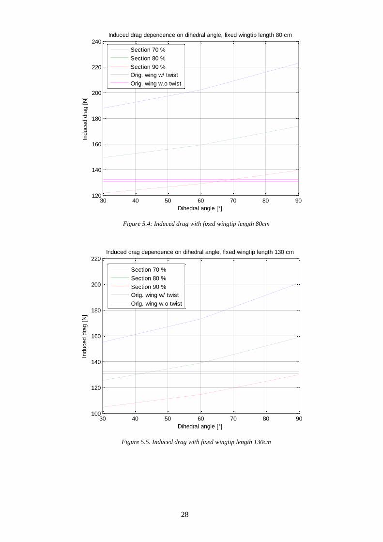
Figure 5.4: Induced drag with fixed wingtip length 80cm

Figure 5.5. Induced drag with fixed wingtip length 130cm

30 40 50 60 70 80 90120

140

160

180

200

220

240Induced drag dependence on dihedral angle, fixed wingtip length 80 cm

Dihedral angle [°]

Induced d

rag [

N]

Section 70 %

Section 80 %

Section 90 %

Orig. wing w/ twist

Orig. wing w.o twist

30 40 50 60 70 80 90100

120

140

160

180

200

220Induced drag dependence on dihedral angle, fixed wingtip length 130 cm

Dihedral angle [°]

Induced d

rag [

N]

Section 70 %

Section 80 %

Section 90 %

Orig. wing w/ twist

Orig. wing w.o twist

29

After testing the three lengths of winglets at different positions along the wing and with varying

dihedrals, one more set of tests are done on the wing. Here the lengths of the winglets are

modified so that the root bending moment constraint is fulfilled at each wing position and

dihedral. The following graph shows the resulting induced drag:

Figure 5.6. Induced drag with varying length limited to max. bending moment

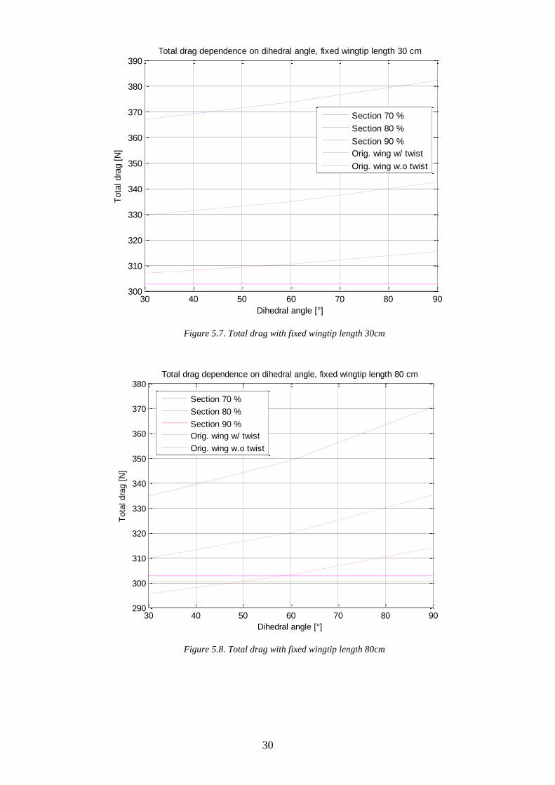
After the induced drag is analyzed, it is a good idea to look at the total drag that results from the

same winglet tests. From the above theory, a decrease in induced drag does not automatically

account for a decrease in the total drag. The following graphs show how the total drag is affected

by the same varying winglet modifications:

30 40 50 60 70 80 90110

115

120

125

130

135

140Induced drag dependence on dihedral angle, maximum wingtip length satisfying bending moment constraint

Dihedral angle [°]

Induced d

rag [

N]

Section 70 %

Section 80 %

Section 90 %

Orig. wing w/ twist

Orig. wing w.o twist

30

Figure 5.7. Total drag with fixed wingtip length 30cm

Figure 5.8. Total drag with fixed wingtip length 80cm

30 40 50 60 70 80 90300

310

320

330

340

350

360

370

380

390Total drag dependence on dihedral angle, fixed wingtip length 30 cm

Dihedral angle [°]

Tota

l dra

g [

N]

Section 70 %

Section 80 %

Section 90 %

Orig. wing w/ twist

Orig. wing w.o twist

30 40 50 60 70 80 90290

300

310

320

330

340

350

360

370

380Total drag dependence on dihedral angle, fixed wingtip length 80 cm

Dihedral angle [°]

Tota

l dra

g [

N]

Section 70 %

Section 80 %

Section 90 %

Orig. wing w/ twist

Orig. wing w.o twist

31

Figure 5.9. Total drag with fixed wingtip length 130cm

Just as the above tests, the lengths of the winglets were modified so that the root bending

moment constraint was fulfilled at each wing position and dihedral. In the graph bellow, Figure

5.10, the total drag can be seen for the same winglet modifications as in Figure 5.6:

Figure 5.10. Total drag with varying length limited to max. bending moment

30 40 50 60 70 80 90290

300

310

320

330

340

350

360

370Total drag dependence on dihedral angle, fixed wingtip length 130 cm

Dihedral angle [°]

Tota

l dra

g [

N]

Section 70 %

Section 80 %

Section 90 %

Orig. wing w/ twist

Orig. wing w.o twist

30 40 50 60 70 80 90300

320

340

360

380

400

420Total drag dependence on dihedral angle, maximum wingtip length satisfying bending moment constraint

Dihedral angle [°]

Tota

l dra

g [

N]

Section 70 %

Section 80 %

Section 90 %

Orig. wing w/ twist

Orig. wing w.o twist

32

6 DISCUSSION AND CONCLUSIONS

6.1 Discussion

The following discussion has been split into three topics to help the reader understand what has

been discussed throughout the project. The first topic will take the reader through a time line of

how the project has been tackled. Next, the reader will get an in depth explanation on how the

results of the project are interpreted. Finally, the reader will get an array of recommendations for

alternative tests that may help in future testing of winglets.

6.1.1 Project History

Designing and comparing wings in XFLR5 has not been an easy task. Throughout the project

there has arisen several hinders that have taken energy to overcome. From the beginning,

learning XFLR5 and all of its functions has been time consuming. There is little information to

be found about the program in modern day literature. Most of the learning within the program

has been gained from trial and error, as well as reading tips in discussion boards online.

Everything from modern winglet design to twist distribution had to be discussed in order to

properly execute this project.

From the start, the idea was to design a modified wing for a general aviation aircraft that could

easily be applied and would greatly reduce drag. The goal was to reduce the total drag on the

wing, while giving it the optimum lift force at a steady level flight. This would in turn minimize

fuel consumption, increase flying distance, and reduce air pollution. Here it was decided that a

Cessna 172 would be the airplane of choice.

The original thought process was that with the help of winglets on the wing, the above goals

could be reached. Here the idea was to design the best winglet possible to apply to a Cessna 172

wing that would reduce drag without affecting the skeleton of the airplane. In turn, this meant

that Cessna would have a cheap and easy application to their design that would benefit both the

customer and the company economically.

Several problems began to take form after further thought. The main problem being that it is

extremely hard to find detailed plans of the entire Cessna 172 as well as it would be difficult to

implement in XFLR5. Here, the idea was born to only focus on the wing of the Cessna 172. By

shifting the focus to only looking at the wing, the project began to center more on the

aerodynamics of the wing instead of the design aspect of building a wing. Attention was now set

on studying the effects winglets have on the lift to drag ratios on the airplane wing. A goal was

set to modify the Cessna 172 wing to have an optimum lift to drag ratio.

After reading several articles and studying earlier projects involving winglets, it became clear

that it would be hard to see any positive effects on the Cessna 172 wing without having to

greatly modify the original structure. What felt like an infinite amount of possibilities began to

surface; it was now time to limit the wing design in order to fit it into the slotted time limit given

for the project. Here the root bending moment constraint was defined for the wing, where this

limit may not be passed by more than 0.5%.

Next, it became apparent that the varying wings are harder to compare than originally thought.

From the start, most of the focus was set on looking at the lift and drag coefficients, CL and CD.

It later became clear that only comparing the coefficients was not enough to gain a full

understanding if the effects are positive or not. This is mainly due to the wing areas changing as

the winglets changed, as seen in Equation (2.16). To solve this, it was decided that XFLR5 was

to be analyzed a bit differently. As read earlier in Method, the forces are looked at directly,

33

instead of studying the coefficients. The mass of the plane was assumed constant, even after

winglet changes, this lead to a constant lift that is used for all of the wing modifications.

Lastly, it was determined that it was best to divide the results into looking at induced drag and

total drag. The goal officially being that one wants to study a set of different winglets to see their

effects on induced drag, as well as seeing the net total effect on drag.

6.1.2 Result Discussion From the earlier graphs in Results, one can see that most of the predefined tests do not fulfill the

requirements for a reduced induced drag for a given constant lift. In Figure 5.4 and Figure 5.5 it

looks as if there are three situations where the wings have less induced drag than the original

twisted wing. These points are for the wing set-ups:

1. 30° winglet with 80cm length at a 90% section of the wing.

2. 30° winglet with 130cm length at an 80% section of the wing.

3. 30° winglet with 130cm length at a 90% section of the wing.

A closer look at the bending moments at these three points shows that the bending moments at

the root chord exceeds the previously defined 1% limit. Therefore, all of the 27 tests seen in

Table 4.3 in Method do not accomplish the task of reducing induced drag without surpassing the

root bending moment constraint. Upon further examination of the total drag from these varying

wingtips that fulfill the bending moment requirements, it can be seen that there is no net benefit

to the total drag due to the new wingtips. The total drag increases for all of these modifications.

In Figure 5.6, it can be seen that there are winglet length/angle combinations that do meet the

previously set requirements for induced drag. The lengths of the winglets have been maximized

for every new winglet angle and position so that the bending moment limit is not passed. Here,

the following four combinations result in a Cessna 172 wing with applied winglets that has a

reduced induced drag:

Figure 6.1. 60° winglet with 255cm length at a 70% section of the wing

34

Figure 6.2. 90° winglet with 565cm length at a 70% section of the wing

Figure 6.3. 60° winglet with 160cm length at an 80% section of the wing

35

Figure 6.4. 90° winglet with 300cm length at an 80% section of the wing

From the above figures as well as the total drag graphs in Results, it can be seen that these wings

are not optimum. The total drag graphs show that although there is a decrease in induced drag,

the effects on total drag are still negative. Both the original wing with twist, and the original

wing without twist have less total drag than all of the modified maximum winglets. In the above

images, one can see that with the exception of Figure 6.3, the winglets look unproportional.

When applied to real world situations, these wings would most likely be oversized or too tall for

standard general aviation hangars or transports.

Another interesting aspect that can be seen in Figure 5.6 is that it could exist an optimal dihedral

angle that minimizes the induced drag for a given root bending moment. This type of winglet

design, where the winglet length is increased until the bending moment is maxed, is only valid

under the given conditions. As seen in the graph, the induced drag for all three sections look to

be at a minimum at 60°. This may be a form of minimum point for varying winglet lengths,

although further testing should be done at more dihedral angles to see at which angle winglets

have the best effect.

After all of the tests and modifications that could be done within the time given, the best design

for a Cessna 172 wing would be the original twisted wing without winglets, that is, the same

wing that is currently used. As for induced drag, it is seen that for an increased length in wing or

winglet there is a decrease in induced drag. Although, as the wing length increases, the bending

moment will increase along the wing. This may result in a restructuring of the wing to

compensate for the added bending moment, which in turn most likely will add weight, and

decrease the net benefit of the new wing. The above results look to match the earlier Theory

chapter. For the tests done in this project, induced drag could be reduced, but the total drag was

not beneficial.

6.1.3 Alternative Tests As discussed above, even if the total drags for the new winglets were not reduced, potential for

improvement can still be seen. Although the main goal of the project was to view the effects

36

winglets have on drag, one may want to use this project as a building block for better winglet

design for future aircrafts. One can go back and begin to alter and re-test many of the parameters

and variables that have been defined throughout the project. A few recommendations for future

testing may include:

New and better winglet designs

Increase in bending moment limits

Varying twist distributions along the wing and winglets

Different flight conditions

More detailed winglet junctions

Another interesting aspect would be to design a new wing with winglets already in mind. The

project has focused on applying winglets to an already optimized planar wing. Improving the

performance of an already effective wing has proved to be challenging. Therefore, it may be

easier to design a new wing that has winglets integrated from the beginning. There is more room

for adjustment, and the above recommendations can be tested more thoroughly.

6.2 Conclusions

It is no easy task to design and fit a winglet to an existing wing. Extending the wing lengths do

result in a decrease in induced drag, although at the expense of increasing the wetted area of the

wing. This results in an increase in total drag due to factors such as parasitic drag and

inconsistencies in the junction flows. The dihedral angling of the winglets play an important role

on the effects of drag as well.

Computation programs such as XFLR5 and MATLAB are worthy tools for wing and winglet

testing, although further model testing in wind tunnels or flight tests would be recommended

before making complete conclusions. The computational programs offer a quick and easy

solution to begin testing, as well as to gain an understanding of the effects that modifications

may have on an aircraft.

Careful planning is in order when designing new winglets. Parameters as well as design models

need to be discussed and planned in order to get an effective winglet. Good aerodynamic practice

is a must to avoid an increase in drag. Changing different parameters will result in varying lift

distributions, bending moments, as well as a change in induced drag and total drag. It is

important to make just comparisons when looking at different winglets. If not done correctly, the

compared data for the winglets is inconclusive.

As seen throughout the project, it is possible to decrease the induced drag on a Cessna 172 wing

without surpassing a root bending moment constraint. A good way to make the winglets more

effective is to focus on reducing the induced drag while trying to keep the parasitic drag to a

minimum.

6.3 Division of Labor

The division of labor has been distributed evenly throughout the project. All three group

members have worked together and spent an even amount of time working in XFLR5,

MATLAB, and Microsoft Word. Meetings were set up regularly each week, and all of the work

was done in computer labs at the KTH campus. All three members are therefore equally

responsible for each part of the project process.

37

7 REFERENCES

[1] http://en.wikipedia.org/wiki/Cessna_172

[2] Jane, Fred T. and Jackson, Paul (eds.). Jane’s All The World’s Aircraft. 100th ed. London:

Jane’s Information Group. 2013.

[3] McLean, Doug. Wingtip Devices: What They Do and How They Do It. Boeing -

Aerodynamics, Article 4, 2005.

[4] Milne-Thomson, L. M. Theoretical Aerodynamics. Dover Publications, 4th edition, 1958.

(PAGE 209)

[5] Karlsson, Arne. Lifting-line method results for the lateral twist distribution giving an elliptic

load distribution. Dept. of Aeronautical and Vehicle Engineering, KTH. 2014

[6] Karlsson, Arne. The aeroplane – some basics. Dept. of Aeronautical and Vehicle

Engineering, KTH. 2014

[7] XFLR5 Guidelines, v6.02. 2013. http://sourceforge.net/projects/xflr5/files/, Visited 18 May

2014

[8] Karlsson, Arne. Steady level flight of an aeroplane with propeller propulsion. Dept. of

Aeronautical and Vehicle Engineering, KTH. 2012

[9]

http://www.cessna.com/~/media/Files/Single%20Engine/skyhawk/Skyhawk%202013%20172S

%20SD.ashx, Visited 18 May 2014

[10] U.S. Standard Atmosphere. U.S. Government Printing Office. 1976.

http://ntrs.nasa.gov/archive/nasa/casi.ntrs.nasa.gov/19770009539.pdf, Visited 18 May 2014

[11] http://www.xflr5.com/docs/Point_Out_Of_Flight_Envelope.pdf, Visited 18 May 2014