Wind Turbine Shutdowns and Upgrades in Denmark:Timing Decisions and the Impact of Government Policy∗

Jonathan A. Cook† C.-Y. Cynthia Lin Lawell‡

October 2019

Abstract: For policymakers, an important long-run question related to the development of renewableindustries is how government policies affect decisions regarding the scrapping or upgrading of existingassets. This paper develops a dynamic structural econometric model of wind turbine owners’ decisionsabout whether and when to add new turbines to a pre-existing stock, scrap an existing turbine, or replace oldturbines with newer versions (i.e., upgrade). We apply our model to owner-level panel data for Denmark overthe period 1980-2011 to estimate the underlying profit structure for small wind producers (who constitutethe vast majority of turbine owners in the Danish wind industry during this time period), and evaluate theimpact of technology and government policy on wind industry development. Our structural econometricmodel explicitly takes into account the dynamics and interdependence of shutdown and upgrade decisions,and generates parameter estimates with direct economic interpretations. Results from the model indicate thatthe growth and development of the Danish wind industry were driven primarily by government policies asopposed to technological improvements. We use the parameter estimates to simulate counterfactual policyscenarios in order to analyze the relative effectiveness and cost-effectiveness of the Danish feed-in-tariff andreplacement certificate programs. Results show that both of these policies significantly impacted the timingof shutdown and upgrade decisions made by small wind producers and accelerated the development of thewind industry in Denmark. We also find that when compared with the feed-in-tariff; a declining feed-in-tariff; and the replacement certificate program and the feed-in-tariff combined, the replacement certificateprogram was the most cost-effective policy both for increasing payoffs of small wind producers and also fordecreasing carbon emissions.

Keywords: wind energy, dynamic structural econometric modelJEL codes: Q42, L90

∗The authors are tremendously thankful for the help of Dr. Preben Nyeng at Energinet.dk for his help in understanding theDanish electricity market, access to turbine ownership data, and connections to other experts in the field. We thank David Broad-stock and four anonymous referees for detailed and thoughtful comments that have greatly improved our paper. Estelle Cantillon,Jon Conrad, Thom Covert, Harry de Gorter, Catherine Hausman, Harry Kaiser, Corey Lang, Shanjun Li, Shaun McRae, ArielOrtiz-Bobea, Steve Puller, Dave Rapson, Mar Reguant, Douglass Shaw, Jim Stock, Rich Sweeney, Chad Syverson, Chris Tim-mins, Dmitry Vedenov, Frank Wolak, Richard Woodward, and Andrew Yates provided valuable comments and discussions. Wealso received helpful comments from conference participants at the Stanford Institute for Theoretical Economics (SITE), the Na-tional Bureau of Economic Research (NBER) Summer Institute Environmental and Energy Economics Workshop, the Agriculturaland Applied Economics Association (AAEA) Annual Meeting, the U.S. Association of Energy Economics North American confer-ence, and the Harvard Environmental Economics Program Research Workshop; and from seminar participants at Cornell University,Texas A&M, and the University of California at Davis. All errors are our own.

†Salt River Project, Phoenix, AZ; cooks333@gmail.com‡(Corresponding Author), Dyson School of Applied Economics and Management, Cornell University, 407 Warren Hall, Ithaca,

NY 14853-4203; clinlawell@cornell.edu

1

1 Introduction

Due to concerns about climate change, local air pollution, fossil fuel price volatility, energy security, and

possible fossil fuel scarcity, governments at many levels around the world have begun implementing policies

aimed at increasing the production share of renewables in the electricity sector. These support policies have

taken several different forms (e.g., Renewable Portfolio Standards, feed-in-tariffs, tax credits, etc.), and

proponents argue that they are necessary for these nascent industries to continue to develop technological

improvements, achieve economies of scale, and compete with existing industries. Wind energy was one of

the earliest renewable generation technologies to be promoted, and its maturity and low costs relative to

other renewables have made it a leading option for many countries in the early phases of pursuing climate

goals.

For policymakers, an important long-run question related to the development of renewable industries

is how government policies affect decisions regarding the scrapping or upgrading of existing assets. How

much of the shutdowns and upgrades can be attributed to the policies as opposed to technological progress?

How do policies affect the timing of owner decisions and the subsequent path of the industry?

This paper aims to shed some light on these questions by developing a dynamic structural econometric

model of wind turbine shutdowns and upgrades in the context of Denmark and using it to estimate the

underlying profit structure for turbine owners. In particular, we model wind turbine owners’ decisions about

whether and when to add new turbines to a pre-existing stock, scrap an existing turbine, or replace old

turbines with newer versions (i.e., upgrade). Shutting down and/or upgrading existing productive assets are

important economic decisions for the owners of those assets and are also the fundamental decisions that

underlie the development of new, growing industries.

To date, empirical research addressing the economics of wind energy has tended to focus on production

costs, investment decisions, or policy options for increasing the penetration of wind energy in electricity

grids. Engineering studies have regularly calculated the cost of producing electricity from wind turbines

and compared it with existing fossil-fuel generators (Darmstadter, 2003; Krohn et al., 2009). Trancik et al.

(2015) describe the evolution of wind energy in recent decades, and find that wind energy is now nearly

cost-competitive with natural gas- and coal-fired power plants in many regions of the world. Hartley and

Medlock (2017) find that until fossil fuels are abandoned, however, the price of energy is insufficient to

cover even the operating costs of renewable energy production, let alone provide a competitive return on the

capital employed. Krekel and Zerrahn (2017) analyze whether the presence of wind turbines has negative

externalities for people in their surroundings, and find that negative externalities exist but are spatially and

temporally limited; Lang et al. (2014) find that wind turbines have no statistically significant negative im-

pacts on house prices. Jacobsson and Johnson (2000) come at the problem from a technology innovation and

diffusion perspective, and provide an analytical framework for examining the process of technical change

in the electricity industry. Hartley (2018) examines the costs of replacing fossil fuels by wind generation

and storage, and compares wind power with generation based on nuclear and storage. Oliveira et al. (2019)

present an empirical analysis of the displacement of CO2 emissions associated with wind generation in the

Irish electricity market.

Previous studies of scrapping decisions in the electricity industry have been either analytic, numerical,

2

or reduced-form. Fleten et al. (2017) use a numerical real options analysis to study the effects of regulatory

uncertainty and cash flow uncertainty on decisions to shut down, start up, and abandon existing peak power

plants; we build on the methods used by Fleten et al. (2017) by estimating a dynamic model econometrically.

Mauritzen (2014) estimates a reduced-form model of wind turbine scrapping decisions; we build on the work

of Mauritzen (2014) by developing and estimating a dynamic structural econometric model, by utilizing

additional data, by extending the model to include both shutdown and upgrade decisions, and by analyzing

the effects and cost-effectiveness of government policy.

The previous literature on wind policy has been aimed at describing the policies that have been imple-

mented (Allison and Williams, 2010); evaluating different wind energy policies based on their ability to

promote new investments (Agnolucci, 2007; May, 2017), wind production (Aldy et al., 2019), or innovation

(Covert and Sweeney, 2019); examining whether current policies encourage investments in socially optimal

renewable capacity additions (Novan, 2015); or comparing the policies of different countries with emerging

wind industries (Klaassen et al., 2005). Hitaj (2013) analyzes the effects of government policies on wind

power development in the United States. Ciarreta et al. (2017) compare feed-in-tariffs and tradable green

certificates in the Spanish electricity system. Munksgaard and Morthorst (2008) provide an excellent de-

scription of the trends in feed-in-tariffs and the market price of electricity in Denmark, and forecast future

investments in wind energy based on an estimated internal rate of return. Fell and Linn (2013) use a simula-

tion model to compare the cost-effectiveness of renewable electricity policies, including renewable portfolio

standards, production subsidies, and feed-in-tariffs, in the Electricity Reliability Council of Texas (ERCOT)

region. Reguant (2019) analyzes the efficiency and distributional implications of large-scale renewable poli-

cies, including carbon taxes, feed-in-tariffs, production subsidies, and renewable portfolio standards, using

data from the California electricity market.

The “bottom-up” style of modeling we use in this paper is in direct contrast to many previous “top-

down” approaches to examining trends in the wind industry, and the structural nature of our model gives

insights into key economic and behavioral parameters. Understanding the factors that influence individual

decisions to invest in wind energy and how different policies can affect the timing of these decisions is

important for policies both in countries that already have mature wind industries, as well as in regions of the

world that are earlier in the process of increasing renewable electricity generation (e.g. most of the U.S.).

We apply our dynamic structural econometric model to owner-level panel data for Denmark over the

period 1980-2011 to estimate the underlying profit structure for small wind producers (who constitute the

vast majority of turbine owners in the Danish wind industry during this time period), and evaluate the

impact of technology and government policy on wind industry development. Our structural econometric

model explicitly takes into account the dynamics and interdependence of shutdown and upgrade decisions,

and generates parameter estimates with direct economic interpretations.

Results from our dynamic structural econometric model indicate that the growth and development of the

Danish wind industry were driven primarily by government policies as opposed to technological improve-

ments. We use the parameter estimates to simulate counterfactual policy scenarios in order to analyze the rel-

ative effectiveness and cost-effectiveness of the Danish feed-in-tariff and replacement certificate programs.

Results show that both of these policies significantly impacted the timing of shutdown and upgrade decisions

3

made by small wind producers and accelerated the development of the wind industry in Denmark. We also

find that when compared with the feed-in-tariff; a declining feed-in-tariff; and the replacement certificate

program and the feed-in-tariff combined, the replacement certificate program was the most cost-effective

policy both for increasing payoffs of small wind producers and also for decreasing carbon emissions.

The balance of our paper proceeds as follows. We describe the Danish wind industry in Section 2. We

describe our dynamic structural econometric model in Section 3. We present the results in Section 4. Section

5 concludes.

2 The Danish Wind Industry

For many countries, questions regarding wind turbine shutdown and upgrade decisions will become increas-

ingly relevant in the near future as existing turbines approach the end of their expected lifetimes (usually

around 20 years) and technology continues to improve. This is already the case in Denmark, where a con-

certed effort to transition away from fossil fuels began in the late 1970’s soon after the first oil crisis. Since

then, the long-term energy goal of the Danish government has been to have 100% of the country’s energy

supply come from renewable sources.

With a long history of designing turbines that stretches back to the late 19th century (Heymann, 1998),

wind power was Denmark’s leading technological choice to offset electricity production from fossil fuels.

To this end, the Danish government implemented several policies designed to encourage wind investments

throughout the country. As a result of this sustained policy goal, Denmark became a leader in both turbine

design and installed wind capacity during the 1980s and 1990s, and has one of the most mature modern

wind industries in the world. Denmark has dominated other countries in wind deployment per capita and

per GDP, and currently produces the equivalent of roughly 40% of its electricity demand in wind power

(Trancik et al., 2015).

We focus on the wind industry in Denmark over the period 1980-2011, and use data from a publicly

available database containing all turbines constructed in Denmark during that time period (DEA, 2018).

Ownership information for each turbine was obtained from a professional colleague at Energinet.dk so

that a panel data set at the owner level could be constructed and used to estimate our dynamic structural

econometric model. During our period of study, there were significant improvements in turbine technology

as well as changes to government wind policies.

An interesting feature of Danish wind development was that it was not led by a few large firms construct-

ing large, centralized wind farms. Instead, the vast majority of wind turbines in the country were installed

and owned by individuals or local cooperatives. In terms of ownership, the Danish wind industry has been

remarkably decentralized throughout its history. This decentralized development resulted in 80% of all tur-

bines in Denmark being owned by wind cooperatives in 2001 (Mendonca et al., 2009). Of the roughly 2,900

turbine owners during over the period 1980-2011, the vast majority (∼90%) own two or fewer turbines, and

these turbine owners owning two or fewer turbines produced the majority (56.5%) of Denmark’s wind pro-

duction output during this time period. In particular, of the 2,924 total turbine owners in the country during

our period of study (1980-2011), 2,565 (88%) own two or fewer turbines. We therefore focus on turbine

4

owners who own two or fewer turbines.

Our analysis makes use of several turbine-specific and national level variables that likely have an impact

on turbine management decisions. Included in the Energinet.dk data are the capacity of each turbine, the date

it was installed, and the location of the turbine. Capacity enters directly into all specifications of our model,

while the installation date is used to calculate the age of each turbine throughout the study period. Summary

statistics for the capacity and installation date of the turbines we use in our dynamic structural econometric

model (i.e., turbines owned by owners with two or fewer turbines over the period 1980 to 2011) are shown

in Table 1. We also include variables for government policy and for the state of wind turbine technology,

each of which we describe in detail below.

2.1 Government Policy

We focus on two important policies that the Danish government has implemented on the wind industry: (1)

the feed-in-tariff for electricity generated by wind turbines, and (2) the replacement certificate scheme for

incentivizing turbine owners to scrap old turbines and replace them with new ones.

Since the late 1970s, the Danish government has supported wind development by paying wind turbine

owners a feed-in-tariff for electricity generated by wind turbines. A feed-in-tariff is a policy that guarantees

a flat price to renewable technologies for each unit of electricity generation, usually over a long period of

time, potentially with a changing tariff over time and targeted to specific technologies (Fell and Linn, 2013;

Reguant, 2019).

Prior to the liberalization of the power market in 1999,1 the feed-in-tariff provided by the Danish gov-

ernment to wind turbine owners was a fixed price guaranteed for a significant portion (if not all) of a wind

turbine’s useful life. After liberalization,2 the feed-in-tariff was a supplement to be paid to owners on top

of the electricity price determined in the competitive wholesale market so that wind turbine owners were

guaranteed a maximum total price (feed-in-tariff plus market price). The price guaranteed by the feed-in-

tariff is determined by the date a turbine was built, and has been adjusted over time as more wind power

came online (see Table 2). Because the feed-in-tariff guarantees the price that wind turbine owners will

receive for production, wind turbine owners are insulated from changes in wholesale prices.3 Thus, the

shutdown and upgrade decisions of wind turbine owners are likely to be affected by the price guaranteed by

the feed-in-tariff, and not by wholesale prices.

Also beginning in 1999, the government created a replacement certificate program to incentivize the

upgrading of older, lower capacity turbines to newer, larger turbines. Eligible turbine owners who scrapped

1Before 1999, Danish municipal utilities were vertically integrated and operated as regulated natural monopolies so that theprice of electricity for retail customers was set at a level that allowed the utility to recouperate the cost of generating, transmitting,and distributing electricity to its customers.

2After liberalization in 1999, Denmark joined the Nordic regional market (NordPool) and began using locational marginalpricing together with a Dutch auction mechanism (2nd price auction) to determine wholesale prices. Because the feed-in-tariffguarantees the price that wind turbine owners will receive for production, however, wind turbine owners are insulated from changesin wholesale prices, including those resulting from changes in Nordpool prices and Danish foreign electricity trade.

3Massive increases in wind capacity (and generation) can have an impact on daily wholesale prices. On particularly windy days,the wholesale price can become negative as zero-marginal cost wind becomes the marginal source of generation and the marketactually pays buyers to use excess wind production. Rintamaki et al. (2017) find that wind power decreases the daily volatility ofprices in Denmark, however, by flattening the hourly price profile.

5

their turbines during the program received a certificate that would grant an additional price supplement for a

new turbine that was constructed (see Table 3). These scrapping certificates were given out through the end

of 2011 and could be used by owners to upgrade their turbines (which we define as scrapping an existing

turbine they own and subsequently adding a new turbine in the same year), or sold to other prospective

turbine owners.

Figure 1 graphs the fraction of all owners of one turbine who scrap, add, and upgrade, respectively,

for each year of the data set. Similarly, Figure 2 graphs the fraction of all owners of two turbines who

exit, scrap one turbine, and upgrade, respectively, for each year of the data set. In both figures, the dotted

vertical lines indicate the years in which the feed-in-tariff was high, medium, and low, respectively. The

dashed vertical lines indicate the years when there was no replacement certificate, and the years when the

replacement certificate was high, medium, and low, respectively.

As can be seen in both figures, there is variation over time in fraction of turbine owners who scrap, add,

and upgrade, and also in the relative frequency of each of these decisions. Also as can be seen in both figures,

there is a possible correlation between the decisions of turbine owners and the government policies. In order

to more rigorously analyze the effects of government policies on turbine owners’ decisions, however, one

needs to estimate a dynamic structural model.

From the perspective of turbine owners, the evolution of both of these policies over time was uncertain

at the beginning of the study period, due to the democratic nature of lawmaking and uncertainty about the

evolution of the Danish wind industry and fuel prices for other forms of electricity generation. Although the

basic strategy of reducing the feed-in-tariff over time was likely known by turbine owners, the exact timing

and values of either of the support policies could not have been perfectly anticipated. We therefore model

future values of these policies as uncertain from the point of view of the turbine owners in any given year of

our period of study in our dynamic structural model. In particular, we assume that both of these government

policies evolve as a finite state first-order Markov process, and that a turbine owner’s expectations of future

values of these government policies depend on current values of these policies and on current values of other

state variables, including the state of wind turbine technology. We use empirical probabilities to estimate a

turbine owner’s expectation of future values of these policies conditional on current values of these policies

and on current values of other state variables.

2.2 State of Wind Turbine Technology

For our measure of the state of wind turbine technology in Denmark, we use the levelized cost of energy

in Denmark. Levelized cost of energy is defined as the total present value cost of a turbine divided by the

total amount of electricity it produces in its lifetime. The levelized cost can be thought of as the price that

electricity would have to be sold at in order for a new generator to break even over the lifetime of the project.

It provides a signal to owners about the costs associated with installing a new turbine that year.

Levelized cost is calculated by summing the present discounted value of the entire stream of total costs

of an electricity-generating asset over the course of its expected lifetime, and then dividing by the total

amount of electricity the asset is expected to produce. Total costs include initial capital costs, fuel costs, and

operation and maintenance costs. Levelized costs are typically calculated over 20-40 year lifetimes, and all

6

costs over this expected lifetime are discounted back to the present.

A general equation for levelized cost lcoe is given by:

lcoe =

∑Tt=1

It+Mt+Ft(1+r)t∑T

t=1 Et, (1)

where, for each time t from t = 1 to t = T , It denotes investment cost, Mt denotes maintenance cost, Ft

denotes fuel cost, Et denotes electricity output at time t, and r is the discount rate. In the case of wind,

fuel costs are zero and operation costs are low, so the bulk of the cost is the cost of the turbine itself. Total

electricity generation (in kWh) is usually estimated by specifying a capacity factor representing the fraction

of time the turbine will actually be producing electricity, and then multiplying that number by the capacity

of the turbine (in kW) and the number of hours in a year (which is 8760 hours).

One of the primary purposes of the levelized cost of energy is to allow developers to evaluate potential

projects on a prospective basis. Though the actual number is very much dependent on the assumptions

that are made, the levelized cost is meant to give an idea of the likelihood of a project breaking even. For

example, if the levelized cost of energy for a potential wind project is a lot higher than the current price of

electricity, then that project does not look very promising.

For our estimates of the levelized cost of wind energy, we use the estimates of the levelized cost of

energy for onshore wind turbines in Denmark from the Danish Energy Agency (DEA, 1999) for each year

over the period 1980 to 1999, which were the years when these estimates were available, and we use the

lower bound of the remaining estimates in Lantz et al. (2012) for each year over the period 2000 to 2010.

We extrapolate the levelized cost for 2011 using data from the years 2004-2010. Figure 3 plots the levelized

costs of wind energy used in our model. For comparison, the levelized costs of producing electricity in

Denmark from combined-cycle gas turbines and from steam turbine extraction generators, as estimated by

Levitt and Sørensen (2014b), are plotted in Figure 3 as well.4

As seen in Figure 3, the levelized costs of wind energy are generally declining over the period 1980

to 2003. During this period, as technology improved over time, the cost of generating electricity from

wind turbines declined because of economies of scale and learning. Beginning around 2003 and continuing

through the latter half of the 2000s, however, wind power capital costs increased, primarily due to rising

commodity and raw materials prices, increased labor costs, improved manufacturer profitability, turbine

upscaling, and demand growth (Lantz et al., 2012; Trancik et al., 2015). As a consequence, the levelized

costs of wind energy increased beginning around 2003 and continuing through the latter half of the 2000s,

in spite of continued performance improvements (Lantz et al., 2012).

Because we eventually discretize the levelized cost of energy into three bins for use in our structural

model, our results are robust to any imprecision in our estimates of the levelized cost of energy owing to our

merging estimates from multiple sources and our extrapolating the values for the year 2011, as any impreci-

sion is unlikely to have large effects on the bin into which the levelized cost of energy in any particular year

4The interest rate used to calculate the levelized costs was the effective bond interest rate (series lwbz) from the StatisticsDenmark Annual Danish Aggregate Model (Statistics Denmark, 2013). These rates date from 1948, providing a consistent set ofinterest rates. It is likely that these interest rates are a little lower than the financing rates actually offered to finance electricitygeneration projects (Levitt and Sørensen, 2014a).

7

falls.

We assume that all turbines built in the same year have the same discretized value of the levelized

cost. As Denmark is a small and topographically homogenous country, the spatial variation in annual wind

patterns is relatively small, so this is a reasonable assumption for the purposes of measuring the state of

technology. According to our preliminary analyses using descriptive reduced-form econometric models of

the decisions of small wind producers in Denmark to add, scrap, or upgrade a wind turbine (not shown),

wind quality generally does not have a significant effect.

The purpose of including levelized cost of energy in our model is to capture the development of wind

turbine technology over time. The idea is that as technology improves, turbine costs will decline and capacity

factors will increase, both of which will lead to a lower levelized cost of energy. As long as the levelized cost

of energy for each year is calculated using similar methodology and assumptions, then what the levelized

cost is capturing is the time path of turbine costs, which is driven by developments in turbine technology.

We are assuming that the levelized cost of energy is exogenous from the point of view of a small wind farm

owner and that an individual owner’s investment decisions do not impact the levelized cost of energy.

We model the future values of technology as uncertain from the point of view of the turbine owners.

Moreover, because we are studying the decisions of turbine owners with small numbers of turbines (rather

than large energy companies), we argue that the evolution of these variables is taken as given by each

individual turbine owner and the owner’s decisions have zero impact on the future values of these variables.

In particular, we assume that the state of wind turbine technology evolves as a finite state first-order Markov

process, and that a turbine owner’s expectations of future values of technology depend on the current state of

technology and on current values of other state variables, including government policies. We use empirical

probabilities to estimate a turbine owner’s expectation of future values of technology conditional on current

values of technology and on current values of other state variables.

Although we assume that an individual wind turbine owner’s investment decisions do not impact either

the levelized cost of energy or government policy, we allow government policies to affect the evolution

of wind turbine technology, and wind turbine technology to affect the evolution of government policy. In

particular, we assume that the state of wind turbine technology evolves as a finite state first-order Markov

process, and that a turbine owner’s expectations of future values of technology depend on the current state

of technology and on current values of other state variables, including government policies. We similarly

assume that both of these government policies evolve as a finite state first-order Markov process, and that a

turbine owner’s expectations of future values of these government policies depend on current values of these

policies and on current values of other state variables, including the state of wind turbine technology. We use

empirical probabilities to estimate a turbine owner’s expectation of future values of government policies and

future values of technology, conditional on current values of government policy, wind turbine technology,

and other state variables.

8

3 Dynamic Structural Econometric Model

We model the decision to add, scrap, or upgrade a wind turbine using a dynamic structural econometric

model. In particular, we develop and estimate a single agent dynamic structural econometric model using

the econometric methods developed in the seminal work of Rust (1987, 1988). These methods have been ap-

plied to analyze various topics including bus engine replacement (Rust, 1987), nuclear power plant shutdown

decisions (Rothwell and Rust, 1997), water management (Timmins, 2002), air conditioner purchases (Rap-

son, 2014), agricultural land use (Scott, 2013), copper mining decisions (Aguirregabiria and Luengo, 2016),

vehicle scrappage decisions (Li and Wei, 2013), agricultural disease management (Carroll et al., 2019a,b,c),

organ transplant decisions (Agarwal et al., 2019), pesticide spraying decisions (Sambucci et al., 2019), ve-

hicle ownership and usage (Gillingham et al., 2016), and the adoption of rooftop solar photovoltaics (Feger

et al., 2017; Langer and Lemoine, 2018).5 To our knowledge, this paper is the first application to the wind

industry.

Applying a dynamic structural econometric model to micro-level data allows one to model the decision

to shut down or upgrade a wind turbine as a dynamic optimization problem at the individual level and enables

one to study the impact of government policies and technological progress on those decisions. This “bottom-

up” style of modeling is in direct contrast to many previous “top-down” approaches to examining trends in

the wind industry, and the structural nature of our model gives insights into key economic and behavioral

parameters. Understanding the factors that influence individual decisions to invest in wind energy and how

different policies can affect the timing of these decisions is important for policies both in countries that

already have mature wind industries, as well as in regions of the world that are earlier in the process of

increasing renewable electricity generation (e.g. most of the U.S.).

There are several advantages to using a dynamic structural model to analyze the shutdown and upgrade

decisions of wind turbine owners. First, unlike reduced-form models, a structural approach explicitly mod-

els the dynamics of shutdown and upgrade decisions. Wind turbines are long-term productive assets that

degrade over time and are costly to replace in terms of money, time, and effort. With an existing turbine,

owners are locked into a fixed output capacity and feed-in-tariff. Meanwhile, technology and government

policies are changing over time. Because the payoffs from shutting down or upgrading turbines depend

on market conditions such as the state of technology and government policies that vary stochastically over

time, a turbine owner who hopes to make a dynamically optimal decision would need to account for the

option value to waiting before making an irreversible decision to shut down or upgrade a turbine (Dixit and

Pindyck, 1994). Using a dynamic model allows an owner’s decision to scrap or upgrade a turbine to be

based not only on the condition of the existing turbine, but also on the current and expected future states of

technology and policy.

A second advantage of the structural model is that with the structural model we are able to estimate

5In addition, structural econometric models of dynamic games have been applied to such issues relating to the environment andenergy as offshore petroleum production (Lin, 2013), environmental regulation (Ryan, 2012), market-based emissions regulation(Fowlie et al., 2016), utility regulation (Lim and Yurukoglu, 2018), renewable fuel subsidies (Yi et al., 2019), the solar industry(Gerarden, 2019), the world petroleum market (Kheiravar et al., 2019; Kheiravar and Lin Lawell, 2019), ethanol investment (Thomeand Lin Lawell, 2019; Yi and Lin Lawell, 2019a,b; Lin Lawell, 2017), climate change policy (Zakerinia and Lin Lawell, 2019), andthe coal industry (Jha, 2019).

9

the effect of each state variable on the expected payoffs from shutting down or upgrading a turbine, and

are therefore able to estimate parameters that have direct economic interpretations. Unlike reduced-form

models, a dynamic structural model accounts for the continuation value, which is the expected value of the

value function next period. With the structural model we are able to estimate parameters in the payoffs from

shutting down or upgrading, since we are able to structurally model how the continuation values relate to

the payoffs from shutting down or upgrading.

A third advantage of our structural model is that we are able to model the interdependence of the shut-

down, addition, and upgrade decisions. In particular, we model the value function for owners of one turbine

and the value function for owners of two turbines separately, but allow them to depend on each other. Since

an owner of one turbine has the option of becoming an owner of two turbines by adding a new turbine, the

value of being an owner of one turbine depends in part on the value of being an owner of two turbines.

Similarly, since an owner of two turbines has the option of becoming the owner of one turbine by scrapping

one of his turbines, the value of being an owner of two turbines depends in part on the value of being an

owner of one turbine.

Modeling the interdependence of the shutdown, addition, and upgrade decisions is particularly important

for analyzing the effects of government policy, since part of the effect of government policies may be owing

to the interdependence of these decisions. For example, part of the effect of the replacement certificate may

be that it increases the shutdown of one turbine by owners of two turbines since it gives them the option of

adding a new turbine in the future, and therefore the option of redeeming the replacement certificate they

earned by the initial shutdown. Similarly, part of the effect of both the feed-in-tariff and the replacement

certificate may be that they increase the addition of a second turbine by owners of one turbine, since doing

so gives them the option of shutting down their older turbine and earning a replacement certificate.

A fourth advantage of our structural model is that we can use the parameter estimates from our structural

model to simulate various counterfactual policy scenarios. In order to analyze the relative effectiveness and

cost-effectiveness of the Danish feed-in-tariff and replacement certificate programs, we use our estimates to

simulate the Danish wind industry in absence of government policy, and compare the actual development

of the industry in the presence of government policy with this counterfactual development in the absence of

policy.

A fifth advantage of using a dynamic structural model to analyze the effects of government policy on

shutdown and upgrade decisions of wind turbine owners is that, although other countries have implemented

policies aimed at increasing the production share of renewables in the electricity sector, it is not clear that a

comparison group exists for any single country that has implemented such policies, and thus a difference-

in-differences approach may not be feasible. Moreover, a country’s renewable energy policy often consists

of multiple policies, and it is valuable to understand which policy in the portfolio is the most influential. A

dynamic structural model is thus well-suited for analyzing the the effects of government policy on shutdown

and upgrade decisions of wind turbine owners.6

6A potential drawback of structural econometric models is that they require sources of structure (e.g., from economic the-ory) and the assumptions underlying these sources of structure may or may not hold in reality. We mitigate these concerns byimposing minimal, parsimonious assumptions in our dynamic structural econometric model of turbine shutdowns and upgrades.As we explain in more detail below, the sources of economic structure in our dynamic structural econometric model are dynamic

10

Our structural model allows for owners to have up to two turbines at any particular time and the available

actions depend on how many turbines are in operation. As mentioned, 88% of turbine owners own two or

fewer turbines during the period of study (1980-2011).

We build upon previous structural dynamic models by modeling two interdependent value functions,

reflecting interdependent shutdown, adding, and upgrading decisions. The basic idea is to have a model

with two “worlds”, such that an owner is in the one-turbine world when he/she has one operating turbine,

and moves to the two-turbine world if and when a second turbine becomes operational. The interdependence

of the shutdown, adding, and upgrading decisions is depicted in Figure 4. We model the decisions of owners

beginning in the year in which their first wind turbine was built, conditional on having built a turbine, so

that all owners begin in the one-turbine world. Each period (year), an owner of one turbine decides whether

to continue producing with a single turbine, add a new turbine, upgrade to a new turbine, or scrap their

existing turbine (exit the market). Scrapping a turbine and adding a turbine in the same period constitutes

an upgrade. If the owner decides to add, then they move to the two-turbine world in the following period,

where they have a slightly different set of possible actions.

In the two-turbine world, owners can either continue producing with two turbines, scrap one of their

existing turbines, upgrade one of their existing turbines, or scrap both of their turbines. Scrapping a turbine

and adding a turbine in the same period constitutes an upgrade. If an owner of two turbines scraps a single

turbine, he/she moves back to the one-turbine world.

Each agent in our model is a turbine owner who owns and operates no more than two wind turbines in

any given period. Each discrete time period t represents a year. In each period t, the each turbine owner i

choices an action di,t ∈ {0, 1, 2, ..., 9}. The choice set available to agent i depends upon the world that an

owner is in during that period, as listed in Table 4. In each period t, an owner of one turbine can decide to

continue without any shutdown, addition, or upgrade; add a small turbine; add a medium turbine; add a large

turbine; upgrade to a small turbine; upgrade to a medium turbine; upgrade to a large turbine; or scrap his

turbine. In each period t, an owner of two turbines can decide to continue without any shutdown or upgrade;

upgrade one turbine to a small turbine; upgrade one turbine to a medium turbine; upgrade one turbine to a

large turbine; scrap one turbine; or scrap both turbines.

The per-period payoff of each each turbine owner i, which measures the turbine owner i’s utility in a

given period t, depends on the action di,t chosen by turbine owner i, the state variables xi,t, and turbine owner

i’s private information shocks εi,t at time t. The per-period payoff (or utility) of a turbine owner includes

anything and everything the turbine owner may care about, including both economic and non-economic

sources of utility. Our model therefore captures both economic and non-economic motives for adding,

scrapping, or upgrading a wind turbine.

The sources of economic structure in our dynamic structural econometric model are dynamic program-

programming and our modeling of the interdependence of the scrapping, adding, and upgrading decisions. Aside from dynamicprogramming and the interdependence of the scrapping, adding, and upgrading decisions, we impose minimal additional assump-tions on our model. For example, our specification of the per-period payoff function is agnostic about the actual functional formof the payoff function; the actual functional form of the production function; the actual functional form of the cost function; theactual nature of the constraints; and the actual mechanism by which, for example, the age of the turbine affects wind production,revenue, costs, and/or payoffs; and thus is general enough to capture the reduced-form implications of a number of models of windproduction, wind energy market behavior, and electricity market behavior.

11

ming and our modeling of the interdependence of the scrapping, adding, and upgrading decisions. Since

our focus is on annual scrapping, adding, and upgrading decisions, we do not model daily wind production

explicitly, and therefore use a reduced-form specification for per-period payoffs. We account for the im-

portant factors in a wind turbine owner’s annual scrapping, adding, and upgrading decisions by including

in the payoff function state variables xi,t that affect wind production, revenue, benefits, and/or costs. We

also include shocks εi,t to the payoff function that may reflect shocks to wind production, revenue, benefits,

and/or costs.

We account for the important factors in a turbine owner’s profit maximization decision by including

in the payoff function state variables that affect wind production; state variables that affect revenue; state

variables that affect non-monetary benefits, including any environmental preferences of the turbine owner

and/or Danish electricity consumers; state variables that affect costs; and shocks that reflect uncertainty in

wind production, revenue, benefits, and/or costs. The per-period payoff function therefore includes terms

that are functions of actions, turbine characteristics, economic factors, and government policy. Our specifi-

cation of the per-period payoff function is agnostic about the actual functional form of the payoff function;

the actual functional form of the production function; the actual functional form of the cost function; the

actual nature of the constraints; and the actual mechanism by which, for example, the age of the turbine

affects wind production, revenue, costs, and/or payoffs; and thus is general enough to capture the reduced-

form implications of a number of models of wind production, wind energy market behavior, and electricity

market behavior.

The per-period payoff (or utility) of each turbine owner i in each period t depends on state variables xi,t

that vary across individuals and/or time. Each state variable is discretized based on observed values in the

data. The state variables include the capacity (cap kw1i) of the first turbine, the age (turbine age1i,t) of

the first turbine, the price guaranteed by the feed-in-tariff (orig f it1i) for the first turbine, the levelized cost

(orig lcoe1i) of the first turbine, the capacity (cap kw2i) of the second turbine, the age (turbine age2i,t) of

the second turbine, the price guaranteed by the feed-in-tariff (orig f it2i) of the second turbine, the levelized

cost (orig lcoe2i) of the second turbine, the current period replacement subsidy (rep subsidyi,t), and the

current period levelized cost (lcoet).

Owing to state-space and computational constraints, we are limited in the number of state variables we

can include in our model. We therefore choose as our state variables those variables that are the most im-

portant factors that affect wind production, revenue, non-monetary benefits, and/or costs. Turbine capacity

affects wind production, and therefore affects revenue, non-monetary benefits, and costs. Turbine age cap-

tures various factors that affect the payoffs from operating an individual turbine that evolve as the turbine

ages, including depreciation, whether the turbine investment has been written off and/or paid off, the obso-

lescence of its older technology, and the costs of operation and maintenance. The price guaranteed by the

feed-in-tariff affects the revenue from wind production. The levelized cost of wind energy, our measure of

the state of technology, affects the revenue, non-monetary benefits, and costs of both wind production and

wind turbine upgrades and additions. The replacement subsidy affects the net benefits from shutdowns and

upgrades.

Because the feed-in-tariff guarantees the price wind turbine owners will receive for production, wind

12

turbine owners are insulated from changes in wholesale prices. Thus, the shutdown and upgrade decisions

of wind turbine owners are likely to be affected by the price guaranteed by the feed-in-tariff, and not by

wholesale prices. As a consequence, since we include the price guaranteed by the feed-in-tariff in the payoff

function, there is no need to also include wholesale prices.7

We assume that the state variables evolve as a finite state first-order Markov process. We also assume

that actions that change an owner’s stock of turbines (e.g., add, upgrade, shutdown) take time to complete

and therefore do not affect the values of state variables until the following period. This is a standard assump-

tion in discrete time models, and also reflects the reality that wind turbines cannot be added, upgraded, or

scrapped instantaneously.

For owners of one turbine, the values of the state variables for the second turbine are set to zero. If

and when an owner owning one turbine chooses to add a second turbine, then in the subsequent period, the

state variables for the second turbine are set equal to their respective values at the time the second turbine

is added. If an owner owning two turbines scraps one of his turbines, which in the data is always the older

turbine, then in the subsequent period the state variables for the first turbine take on the values of the state

variables for the second turbine and the state variables for the second turbine are again set to zero.

There is a choice-specific shock εi,t(di,t) associated with each possible action di,t; these choice-specific

shocks are observed by owner i at time t, before owner i makes his time-t action choice, but is never observed

by the econometrician.

Because the model requires discrete data, we bin the action and state variables. The discrete action

choices are explained above and presented in Table 4. The bins used to discretize the state variables are

shown in Table 5. We discretize turbine capacity into three sizes: small, medium, and large. We discretize

turbine age into three bins: young, middle-aged, and old. The price guaranteed by the feed-in-tariff is binned

into its three levels in Table 2: low, medium, and high. The replacement certificate is binned into its three

levels in Table 3: low, medium, and high. We discretize the levelized cost of wind energy into three bins:

low, medium, and high.

Because the variables in our model have been discretized, there are no meaningful units associated with

the variables, payoffs, or value functions; and the payoff and value functions described in the model do

not explicitly measure revenue or profit. Nevertheless, the payoff function does include action and state

variables that affect wind production, revenue, and/or costs.

Although some information in the data is lost by discretizing the variables, and although there are no

meaningful units associated with the variables, payoffs, or value functions, there are several advantages

of having to use discretized variables in our structural model. First, by discretizing the levelized cost of

energy, our measure of the state of technology, our results are robust to any imprecision in our estimates

of the levelized cost of energy owing to our merging estimates from multiple sources and our extrapolating

the values for the year 2011, as any imprecision is unlikely to have large effects on the bin into which the

levelized cost of energy in any particular year falls.

Second, by discretizing turbine age into three bins, our results are robust to any imprecision in converting

7Moreover, data availability and computational constraints unfortunately preclude us from including wholesale electricityprices as an additional state variable.

13

of the actual turbine age in days to turbine age in years, and any idiosyncratic shocks to the time needed

to construct, install, and/or start operating an individual turbine, as any such imprecision or idiosyncratic

shocks are unlikely to have large effects on the bin into which the turbine age of any turbine-year falls.

Third, in discretizing the turbine capacity into three sizes (small, medium, large), we base the cutoffs

for small and medium turbines on the different eligibility cutoffs for various versions of the replacement

certificate policy specified by the Danish government over the time period of our study. This enables us

to focus our analysis of turbine capacity on the aspects of turbine capacity relevant for Danish wind policy

(i.e., whether or not the turbine capacity exceeds the varying eligibility cutoffs), making our results robust

to the exact choice of turbine capacity within our broader size bins, and enabling us to analyze the relative

effectiveness and cost-effectiveness of the Danish feed-in-tariff and replacement certificate programs without

having to finely model every last detail of every daily or hourly aspect of wind production for each and every

individual turbine owner.

Fourth, the wind policies we examine – the Danish feed-in-tariff and replacement certificate programs

– each take on three discrete values over the time period of our analysis, and are therefore already discrete.

Attempting to extrapolate and make these discrete policy variables continuous would introduce noise and

imprecision that may hinder the ability of any empirical analysis to credibly identify the effect of these wind

policies.

Thus, the discretization of our state and action variables is not only necessary for our dynamic structural

econometric model, but also enables us to best identify and analyze the relative effectiveness and cost-

effectiveness of the Danish feed-in-tariff and replacement certificate programs given data availability and

computational constraints, and in a manner robust to any additional assumptions or imprecision that may

be introduced if we were to instead finely model every last detail of every daily or hourly aspect of wind

production for each and every individual turbine owner.

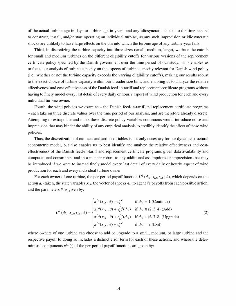
For each owner of one turbine, the per-period payoff function U I (di,t, xi,t, εi,t ; θ), which depends on the

action di,t taken, the state variables xi,t, the vector of shocks εi,t to agent i’s payoffs from each possible action,

and the parameters θ, is given by:

U I (di,t, xi,t, εi,t ; θ)

=

πI,c(xi,t ; θ) + ε I,ci,t if di,t = 1 (Continue)

πI,a(xi,t ; θ) + ε I,ai,t (di,t) if di,t ∈ {2, 3, 4} (Add)

πI,u(xi,t ; θ) + ε I,ui,t (di,t) if di,t ∈ {6, 7, 8} (Upgrade)

πI,e(xi,t ; θ) + ε I,ei,t if di,t = 9 (Exit),

(2)

where owners of one turbine can choose to add or upgrade to a small, medium, or large turbine and the

respective payoff to doing so includes a distinct error term for each of these actions, and where the deter-

ministic components πI, j(·) of the per-period payoff functions are given by:

14

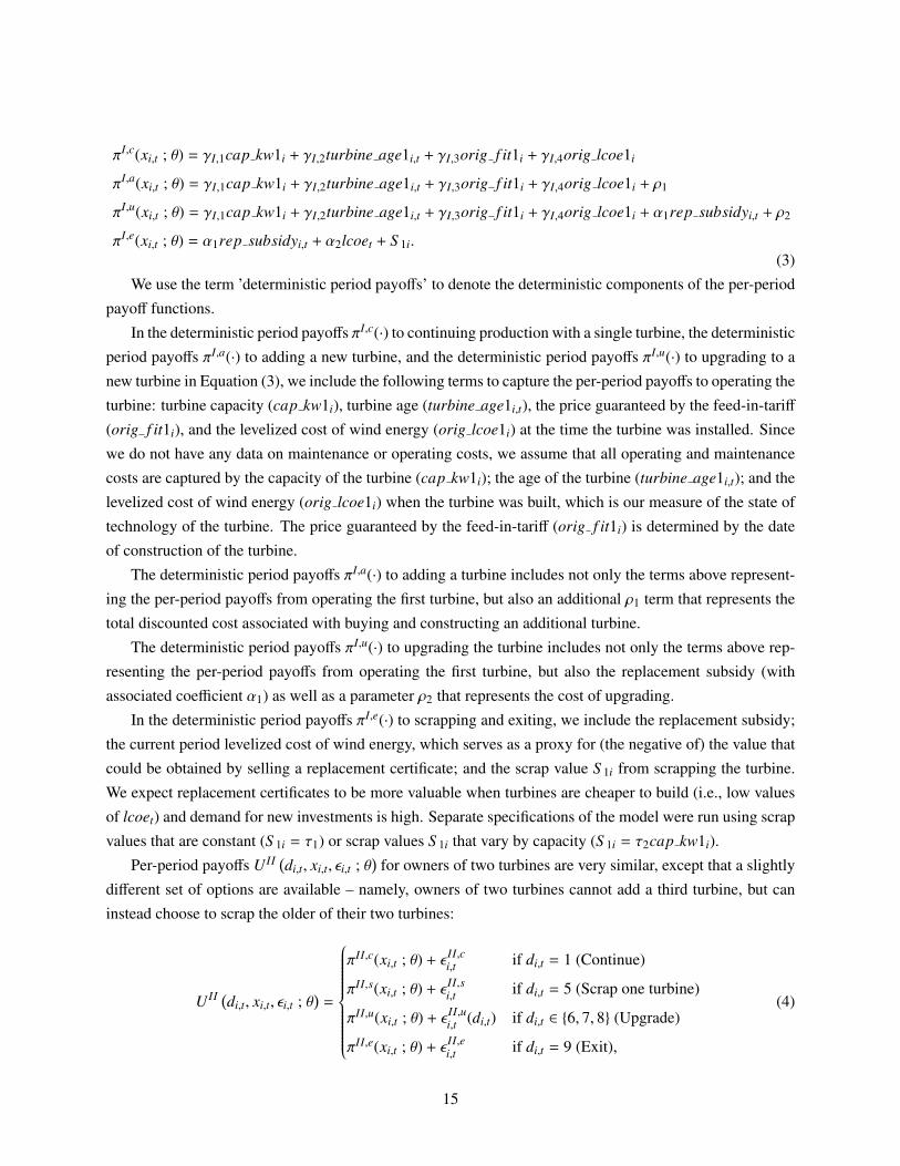
πI,c(xi,t ; θ) = γI,1cap kw1i + γI,2turbine age1i,t + γI,3orig f it1i + γI,4orig lcoe1i

πI,a(xi,t ; θ) = γI,1cap kw1i + γI,2turbine age1i,t + γI,3orig f it1i + γI,4orig lcoe1i + ρ1

πI,u(xi,t ; θ) = γI,1cap kw1i + γI,2turbine age1i,t + γI,3orig f it1i + γI,4orig lcoe1i + α1rep subsidyi,t + ρ2

πI,e(xi,t ; θ) = α1rep subsidyi,t + α2lcoet + S 1i.(3)

We use the term ’deterministic period payoffs’ to denote the deterministic components of the per-period

payoff functions.

In the deterministic period payoffs πI,c(·) to continuing production with a single turbine, the deterministic

period payoffs πI,a(·) to adding a new turbine, and the deterministic period payoffs πI,u(·) to upgrading to a

new turbine in Equation (3), we include the following terms to capture the per-period payoffs to operating the

turbine: turbine capacity (cap kw1i), turbine age (turbine age1i,t), the price guaranteed by the feed-in-tariff

(orig f it1i), and the levelized cost of wind energy (orig lcoe1i) at the time the turbine was installed. Since

we do not have any data on maintenance or operating costs, we assume that all operating and maintenance

costs are captured by the capacity of the turbine (cap kw1i); the age of the turbine (turbine age1i,t); and the

levelized cost of wind energy (orig lcoe1i) when the turbine was built, which is our measure of the state of

technology of the turbine. The price guaranteed by the feed-in-tariff (orig f it1i) is determined by the date

of construction of the turbine.

The deterministic period payoffs πI,a(·) to adding a turbine includes not only the terms above represent-

ing the per-period payoffs from operating the first turbine, but also an additional ρ1 term that represents the

total discounted cost associated with buying and constructing an additional turbine.

The deterministic period payoffs πI,u(·) to upgrading the turbine includes not only the terms above rep-

resenting the per-period payoffs from operating the first turbine, but also the replacement subsidy (with

associated coefficient α1) as well as a parameter ρ2 that represents the cost of upgrading.

In the deterministic period payoffs πI,e(·) to scrapping and exiting, we include the replacement subsidy;

the current period levelized cost of wind energy, which serves as a proxy for (the negative of) the value that

could be obtained by selling a replacement certificate; and the scrap value S 1i from scrapping the turbine.

We expect replacement certificates to be more valuable when turbines are cheaper to build (i.e., low values

of lcoet) and demand for new investments is high. Separate specifications of the model were run using scrap

values that are constant (S 1i = τ1) or scrap values S 1i that vary by capacity (S 1i = τ2cap kw1i).

Per-period payoffs U II (di,t, xi,t, εi,t ; θ)

for owners of two turbines are very similar, except that a slightly

different set of options are available – namely, owners of two turbines cannot add a third turbine, but can

instead choose to scrap the older of their two turbines:

U II (di,t, xi,t, εi,t ; θ)

=

πII,c(xi,t ; θ) + ε II,ci,t if di,t = 1 (Continue)

πII,s(xi,t ; θ) + ε II,si,t if di,t = 5 (Scrap one turbine)

πII,u(xi,t ; θ) + ε II,ui,t (di,t) if di,t ∈ {6, 7, 8} (Upgrade)

πII,e(xi,t ; θ) + ε II,ei,t if di,t = 9 (Exit),

(4)

15

where the deterministic components πII, j(·) of the per-period payoffs are defined as:

πII,c(xi,t ; θ) = γI,1cap kw1i + γI,2turbine age1i,t + γI,3orig f it1i + γI,4orig lcoe1i

+ γII,1cap kw2i + γII,2turbine age2i,t + γII,3orig f it2i + γII,4orig lcoe2i

πII,s(xi,t ; θ) = γII,1cap kw2i + γII,2turbine age2i,t + γII,3orig f it2i + γII,4orig lcoe2i

+ α1rep subsidyi,t + α2lcoet + S 1i

πII,u(xi,t ; θ) = γI,1cap kw1i + γI,2turbine age1i,t + γI,3orig f it1i + γI,4orig lcoe1i

+ γII,1cap kw2i + γII,2turbine age2i,t + γII,3orig f it2i + γII,4orig lcoe2i

+ α1rep subsidyi,t + ρ2

πII,e(xi,t ; θ) = α1rep subsidyi,t + α3lcoet + S 2i.

(5)

In the deterministic period payoffs πII,c(·) to continuing production with two turbines and the determin-

istic period payoffs πII,u(·) to upgrading one of the owner’s existing turbines in Equation (5), we include the

following terms to capture the per-period payoffs to operating the first turbine: turbine capacity (cap kw1i),

turbine age (turbine age1i,t), the price guaranteed by the feed-in-tariff (orig f it1i), and the levelized cost

of wind energy (orig lcoe1i) at the time the first turbine was installed. Since we do not have any data on

maintenance or operating costs, we assume that all operating and maintenance costs for the first turbine are

captured by the capacity of the first turbine (cap kw1i); the age of the first turbine (turbine age1i,t); and the

levelized cost of wind energy (orig lcoe1i) when the first turbine was built, which is our measure of the state

of technology of the first turbine. The price guaranteed by the feed-in-tariff (orig f it1i) for the first turbine

is determined by the date of construction of the first turbine.

The deterministic period payoffs πII,c(·) to continuing production with two turbines and the deterministic

period payoffs πII,u(·) to upgrading one of the owner’s existing turbines include not only the terms above rep-

resenting the per-period payoffs to operating the first turbine, but also the following terms to capture the per-

period payoffs to operating the second turbine: turbine capacity (cap kw2i), turbine age (turbine age2i,t),

the price guaranteed by the feed-in-tariff (orig f it2i), and the levelized cost of wind energy (orig lcoe2i) at

the time the second turbine was installed. Since we do not have any data on maintenance or operating costs,

we assume that all operating and maintenance costs for the second turbine are captured by the capacity of the

second turbine (cap kw2i); the age of the second turbine (turbine age2i,t); and the levelized cost of wind en-

ergy (orig lcoe2i) when the second turbine was built, which is our measure of the state of technology of the

second turbine. The price guaranteed by the feed-in-tariff (orig f it2i) for the second turbine is determined

by the date of construction of the second turbine.

In the deterministic period payoffs πII,s(·) to scrapping one of the owner’s existing turbines, which in

the data is always the older turbine, we include the terms above representing the per-period payoffs to

operating the second turbine; as well as the replacement subsidy; the current period levelized cost of wind

energy, which serves as a proxy for (the negative of) the value that could be obtained by selling a replacement

certificate; and the scrap value S 1i from scrapping the first turbine. Separate specifications of the model were

run using scrap values that are constant (S 1i = τ1) or scrap values that vary by capacity (S 1i = τ2cap kw1i).

16

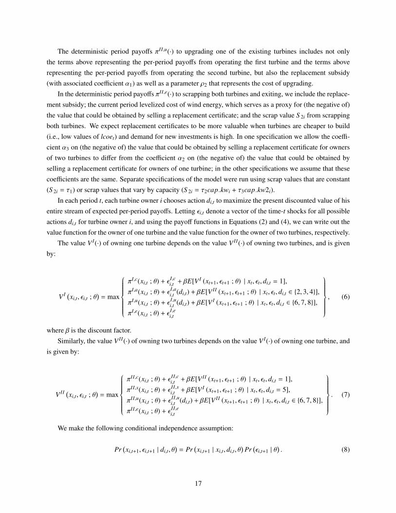
The deterministic period payoffs πII,u(·) to upgrading one of the existing turbines includes not only

the terms above representing the per-period payoffs from operating the first turbine and the terms above

representing the per-period payoffs from operating the second turbine, but also the replacement subsidy

(with associated coefficient α1) as well as a parameter ρ2 that represents the cost of upgrading.

In the deterministic period payoffs πII,e(·) to scrapping both turbines and exiting, we include the replace-

ment subsidy; the current period levelized cost of wind energy, which serves as a proxy for (the negative of)

the value that could be obtained by selling a replacement certificate; and the scrap value S 2i from scrapping

both turbines. We expect replacement certificates to be more valuable when turbines are cheaper to build

(i.e., low values of lcoet) and demand for new investments is high. In one specification we allow the coeffi-

cient α3 on (the negative of) the value that could be obtained by selling a replacement certificate for owners

of two turbines to differ from the coefficient α2 on (the negative of) the value that could be obtained by

selling a replacement certificate for owners of one turbine; in the other specifications we assume that these

coefficients are the same. Separate specifications of the model were run using scrap values that are constant

(S 2i = τ1) or scrap values that vary by capacity (S 2i = τ2cap kwi + τ3cap kw2i).

In each period t, each turbine owner i chooses action di,t to maximize the present discounted value of his

entire stream of expected per-period payoffs. Letting εi,t denote a vector of the time-t shocks for all possible

actions di,t for turbine owner i, and using the payoff functions in Equations (2) and (4), we can write out the

value function for the owner of one turbine and the value function for the owner of two turbines, respectively.

The value V I(·) of owning one turbine depends on the value V II(·) of owning two turbines, and is given

by:

V I (xi,t, εi,t ; θ)

= max

πI,c(xi,t ; θ) + ε I,c

i,t + βE[V I (xt+1, εt+1 ; θ) | xt, εt, di,t = 1],

πI,a(xi,t ; θ) + ε I,ai,t (di,t) + βE[V II (xt+1, εt+1 ; θ) | xt, εt, di,t ∈ {2, 3, 4}],

πI,u(xi,t ; θ) + ε I,ui,t (di,t) + βE[V I (xt+1, εt+1 ; θ) | xt, εt, di,t ∈ {6, 7, 8}],

πI,e(xi,t ; θ) + ε I,ei,t

, (6)

where β is the discount factor.

Similarly, the value V II(·) of owning two turbines depends on the value V I(·) of owning one turbine, and

is given by:

V II (xi,t, εi,t ; θ)

= max

πII,c(xi,t ; θ) + ε II,c

i,t + βE[V II (xt+1, εt+1 ; θ) | xt, εt, di,t = 1],

πII,s(xi,t ; θ) + ε II,si,t + βE[V I (xt+1, εt+1 ; θ) | xt, εt, di,t = 5],

πII,u(xi,t ; θ) + ε II,ui,t (di,t) + βE[V II (xt+1, εt+1 ; θ) | xt, εt, di,t ∈ {6, 7, 8}],

πII,e(xi,t ; θ) + ε II,ei,t

. (7)

We make the following conditional independence assumption:

Pr(xi,t+1, εi,t+1 | di,t, θ

)= Pr

(xi,t+1 | xi,t, di,t, θ

)Pr

(εi,t+1 | θ

). (8)

17

A standard assumption in many dynamic structural models, our conditional independence assumption im-

plies that the evolution of the observed state variables xi,t does not depend on the particular realization of

the idiosyncratic shocks εi,t to the payoffs of individual owners from each possible action choice regarding

upgrading, scrapping, adding, exiting, or continuing.

For turbine age and turbine capacity, the conditional independence assumption makes sense since a

turbine ages will increment by one more year each year regardless of any unobservable idiosyncratic shock

to the individual turbine owner, and since the turbine capacity is chosen by the turbine owner. Moreover,

since we have discretized turbine age and turbine capacity into three bins each, our results are robust to

any imprecision in converting of the actual turbine age in days to turbine age in years, to the exact choice of

turbine capacity within our broader size bins, and to any idiosyncratic shocks to the time needed to construct,

install, and/or start operating an individual turbine, as any such imprecision or idiosyncratic shocks are

unlikely to have large effects on the bin into which the turbine age or turbine capacity of any turbine-year

falls.

For the levelized cost of wind energy, the price guaranteed by the feed-in-tariff, and the replacement

certificate, it is reasonable to assume that shocks to any particular individual turbine owner are unlikely to

affect how industry-level technology and nation-wide government policy evolves at the aggregate level for

all turbine owners.

The transition probabilities Pr(xi,t+1 | xi,t, di,t, θ

)are estimated non-parametrically from the data for all

possible state and action combinations. For turbine age, we kept track of actual age and increment it deter-

ministically each year, then determine which discretized bin the actual age falls into. We assume that each

shock in εi,t is i.i.d. extreme value (type 1) across owners i, actions di,t and time t.

We set the discount factor β to 0.90. Since we focus on small-scale wind turbine owners who own at

most two turbines at any one time in our data set, and do not model larger wind farms, we use the same

discount rate for all turbine owners in our analysis.

As derived in more detail in Appendix A, the probability of a given action conditional on the realization

of a particular combination of state variables is given by the following choice probabilities:

Pr(di,t = d | xi,t, θ

)=

exp(δ j,d

(xi,t, V‡

))∑

d exp(δ j,d

(xi,t, V‡

)) for j = I, II, (9)

where:

δ j,d(xi,t, V‡

)= π j,d + β

∫V‡(xi,t+1)dPr

(xi,t+1 | xi,t, d, θ

)for j = I, II, (10)

and where, as explained in more detail in Appendix A, the ex ante value function V‡ next period used to

calculate the continuation value is either the ex ante value function V I(xi,t+1) for owners of one turbine next

period or the ex ante value function V II(xi,t+1) for owners of two turbines next period, depending upon the

world that an owner is in this period and the action taken this period, and is given by:

V j(xi,t+1) =

∫V j(xi,t+1, εi,t+1; θ)dPr(εi,t+1 | θ) = Eε

[V j(xi,t+1, εi,t+1; θ)

]for j = I, II. (11)

18

After obtaining the model predictions for the choice probabilities as functions of the state variables

and the unknown parameters θ, the parameters θ can then be estimated using nested fixed point maximum

likelihood estimation (Rust, 1987, 1988). The likelihood function is a function of the choice probabilities,

and therefore a function of the ex ante value functions V j for j = I, II. Solving for the parameters θ via

maximum likelihood thus requires an inner fixed point algorithm to compute the ex ante value functions V j

for j = I, II simultaneously as rapidly as possible and an outer optimization algorithm to find the maximizing

value of the parameters θ. In other words, a simultaneous fixed point calculation to compute the ex ante value

functions V j for j = I, II simultaneously is nested within a maximum likelihood estimation (MLE). From

Blackwell’s Theorem, the fixed point for each V j is unique.

Identification of the parameters θ comes from the differences between per-period payoffs across different

action choices, which in infinite horizon dynamic discrete choice models are identified when the discount

factor β and the distribution of the choice-specific shocks εit are fixed (Abbring, 2010; Magnac and Thesmar,

2002; Rust, 1994). In particular, the parameters in our model are identified because each term in the deter-

ministic components πI, j(·) and πII, j(·) of the per-period payoffs given in Equations (3) and (5) for the one-

and two-turbine worlds, respectively, depends on the action di,t being taken at time t, and therefore varies

based on the action taken; as a consequence, the parameters do not cancel out in the differences between

per-period payoffs across different action choices and are therefore identified. For example, the coefficient

γI,1 on the capacity (cap kw1i) of the first turbine in deterministic components πI, j(·) of the per-period pay-

off in the one-turbine world in Equation (3) is identified in the difference between the per-period payoff from

choosing to exit and the per-period payoff from any other action choice di,t.

Standard errors are formed by a non-parametric bootstrap. Turbine owners are randomly drawn from the

data set with replacement to generate 100 independent panels each with the same number of turbine owners

as in the original data set. The structural model is run on each of the panels. The standard errors are then

formed by taking the standard deviation of the estimates from each of the random samples.

The parameter estimates are then used to simulate counterfactual policy scenarios in order to analyze

the relative effectiveness and cost-effectiveness of the Danish feed-in-tariff and replacement certificate pro-

grams.

4 Results

4.1 Structural Parameters

We estimate three specifications of our dynamic structural econometric model. The three specifications vary

in the way they model new turbine costs, scrap values, and the value of selling a replacement certificate.

Specification 1 includes the cost of adding a new turbine costs, the cost of upgrading, and the scrap value

from exiting. Specification 2 allows for the value of replacement certificates to be different for owners of

one turbine and owners of two turbines. Specification 3 assumes that scrap values are proportional to the

size of the turbine.8

8State-space and computational constraints unfortunately limit the number of parameters we are able to estimate in eachspecification, and therefore preclude us from considering alternative combinations of these modeling assumptions that involve

19

The parameter estimates for these three specifications of our dynamic structural econometric model

are reported in Table 6. Because the state variables are discretized, the estimates are not interpretable as

marginal effects, but should instead be interpreted as relative contributions to the profits of turbine owners.

Our estimated coefficients in the per-period payoffs therefore give us a sense of the sign and relative impacts

of different variables on the profits of wind turbine owners and the importance of the policies put into place

by the Danish government.

The positive sign on the coefficient γI,1 in the per-period payoff on the capacity (small, medium, or

large) of the first turbine indicates that higher profits are generated by turbines with higher capacity. The

negative sign on the coefficient γI,2 on the age of the first turbine indicates that the profitability of a turbine

declines with as the turbine gets older. The positive sign on the coefficient γI,3 in the per-period payoff on

the price guaranteed by the feed-in-tariff for the first turbine indicates that higher guaranteed prices yield

higher profits. The negative sign on the coefficient γI,4 on the levelized cost of energy of the first turbine

indicates that the profits are higher if the state of wind turbine technology is better and the levelized cost is

lower. Parameters for owners of one turbine are estimated much more precisely likely due to fact that there

is a relatively small sample of owners owning two turbines.

The positive coefficient α1 in the per-period payoffs on the replacement certificate indicates that the

deterministic period payoffs from upgrading or scrapping are higher when the replacement certificate is

greater. The negative coefficients α2 and α3 on levelized cost of energy in the (the negative of) the value that

could be obtained by selling a replacement certificate in some specifications provide some evidence that, as

expected, replacement certificates are more valuable when turbines are cheaper to build (i.e., low values of

lcoet) and demand for new investments is high.

We find that there are costs to adding new turbines and to upgrading a turbine that are both statistically

significant and large in magnitude. Comparing the magnitudes of the costs of adding (ρ1) and upgrading

(ρ2), we find that upgrading is the more costly of the two actions.

One way to assess the relative importance of government policies as opposed to technological improve-

ments is to compare the relative effects of changes in the discretized values of the government policies and

the state of technology, respectively. Since each of the policy and technology variables has been discretized

into three bins each, changes in their discretized values (e.g., from low to medium, or from medium to high)

reflect comparable changes across the respective distributions of each state variable.

In all specifications, the price guaranteed by the feed-in-tariff is a significant source of revenues. A

change in the price guaranteed by the feed-in-tariff (e.g., from low ($0.06/kWh) to medium ($0.08/kWh), or

from medium ($0.08/kWh) to high ($0.11/kWh)) has approximately 1.5 to 2 times the effects on per-period

payoffs as a decrease in the level of the levelized cost of energy, the indicator of technology (e.g., from high

(> $100/MWh) to medium ($76-100/MWh), or from medium ($76-100/MWh) to low ($0-75/MWh)), where

the levels are determined by the bins in Table 5.

Likewise, replacement certificates comprise a significant share of the payoffs to scrapping or upgrading

existing turbines in all three specifications. A change in the level of the replacement certificate (e.g., from

low ($0.01/kWh) to medium ($0.02/kWh), or from medium ($0.02/kWh) to high ($0.03/kWh)) has approx-

estimating additional parameters.

20

imately 7 to 9.5 times the effects on per-period payoffs as a decrease in the level of the levelized cost of

energy, the indicator of technology (e.g., from high to medium, or from medium to low).

Our results therefore indicate that the growth and development of the Danish wind industry were driven

primarily by government policies as opposed to technological improvements.

To assess the goodness of fit of our models, Table 6 also reports the log likelihood from each of the three

specifications. Our preferred specification is Specification 1, which has the highest log likelihood among

our three specifications.

4.2 Policy Simulations

One of the primary benefits of estimating a structural model is that it enables us to simulate counterfactual

policy scenarios to analyze the relative effectiveness and cost-effectiveness of the Danish feed-in-tariff and

replacement certificate programs. We use our estimates to simulate the Danish wind industry in absence

of government policy, and compare the actual development of the industry in the presence of government

policy with this counterfactual development in the absence of policy.

The particular counterfactual policy scenarios we simulate are the following. In the first counterfactual

policy scenario, we remove the replacement certificate program (but make no changes to the feed-in-tariff).

In the second counterfactual policy scenario, we modify the feed-in-tariff so that the price guaranteed by the

feed-in-tariff declines as a turbine ages as shown in Table 7, instead of remaining flat through the lifetime

of the turbine (but make no changes to the replacement certificate program). In the third counterfactual

policy scenario, we remove the feed-in-tariff (but make no changes to the replacement certificate program).

In the fourth counterfactual policy scenario, we remove both the replacement certificate program and the

feed-in-tariff.

For each counterfactual policy scenario, we use Specification 1 of the model (our preferred specification)

to simulate the effects of the counterfactual policy on wind turbine shutdown and upgrade decisions and the

evolution of the Danish wind industry over the time period of our data set (1980-2011). For the parameter

values in our counterfactual simulations, we use the values of the parameter estimates from Specification 1

for parameters that are significant at a 5% level; and we set the values of the parameters in Specification 1

that are not significant at a 5% level, and therefore do not have a significant effect on wind turbine owners’

payoffs or decisions, to 0.

Each simulation in each counterfactual simulations was run as follows. We first modify the relevant

state variables and transition densities to reflect the counterfactual policy being simulated. Beginning with

the first observed value of the remaining state variables for each owner from the actual data, we simulate the

action for that period by drawing from the choice probabilities and the state variables for the next period by

drawing from the transition probabilities. Based on the state variables drawn for the next period, we then

simulate the action for that period and the state variables for the subsequent period, and so on until the last

year of our data set (2011).

Once the simulated data is created, we calculate various summary statistics for comparison to what

actually happened when both policies were in place. These statistics of interest include the discounted

payoffs (or utility) of small wind producers (i.e., the present discounted value of the entire stream of payoffs

21

over the period 1980-2011 for each turbine owner, summed over all owners of two or fewer turbines), the

number of new turbines added, the number of turbines that were scrapped, the number of upgrades made,

the average age of turbines scrapped, and the number of replacement certificates issued over the period

1980-2011. We also calculate, for the turbines in the final year of the data set (2011), the average age of

these turbines and the distribution of these turbines’ capacities.

For each counterfactual policy scenario, we run 100 independent simulations. The means and standard

deviations are then calculated over the 100 independent simulations for each of the summary statistics.

These means and standard deviations are reported in Table 8.

Examining the results in Table 8, there are several noticeable differences between the policy simulations

and what actually happened when both policies were in place. First, discounted payoffs (or utility) of small

wind producers are significantly higher when both policies are in place than in any of the simulations. This

result suggests that both the replacement certificate policy and feed-in-tariff provided windfall gains to small

wind producers. In particular, discounted payoffs (or utility) of small wind producers would have been 70%

lower if there were no replacement certificate and 95% lower if there were no feed-in-tariff. In the absence

of both policies, discounted payoffs (or utility) of small wind producers would have been 96% lower.

A second result is that in all policy simulations, owners choose to scrap more and add fewer turbines

under the counterfactual scenarios than they do when both policies are in place. This is likely because

the value of owning turbines and the value associated with waiting for future periods before scrapping are

significantly lower in the absence of these policies, since both the replacement certificates and feed-in-tariff

have positive values for turbine owners. As a consequence, many owners scrap their turbines and exit the

industry, rather than add new turbines.

We examine the evolution of the Danish wind industry under the different counterfactual policy scenar-

ios. Figure 5 shows the number of small (< 450 kW), medium (450 - 750 kW), and large (> 750 kW) wind

turbines that existed in each year from 1980-2011 under each policy simulation. Overall, fewer turbines

exist in the simulations except for rapid growth in the number of medium-sized turbines during the boom

years of the industry between 1990-2000.

Our simulation results show that both the replacement certificate policy and feed-in-tariff increased the

discounted payoffs (or utility) of small wind producers. To analyze the relative effectiveness and cost-

effectiveness of the Danish feed-in-tariff and replacement certificate programs, we conduct back-of-the-

envelope calculations to estimate the costs of each of the policies to the Danish government (and therefore

to Danish taxpayers) and well as the carbon emissions benefits of each of the policies, and then compare the

benefits with the costs.

We also calculate the cost-effectiveness of each policy as the cost to the Danish government (and there-

fore to Danish taxpayers) per percentage point increase in discounted payoffs (or utility) of turbine owners,

as well as the cost to the Danish government (and therefore to Danish taxpayers) per million tonne CO2

emissions avoided. This parsimonious analysis of costs and benefits thus enables us to compare the cost-

effectiveness of each policy in achieving two possible objectives of wind policy – increasing payoffs of

turbine owners, and decreasing greenhouse gas emissions – without having to make possibly subjective as-

sumptions about the relative importance of these objectives, the external costs of carbon emissions, and/or

22

the marginal cost of public funds.9 As explained in more detail below, we also use our back-of-the-envelope

estimates of costs and benefits to calculate the minimum threshold discounted payoffs per wind turbine

producer needed in the absence of any policy in order for each policy to be efficient, and the minimum

threshold discounted payoffs per wind turbine producer needed in the absence of any policy in order for

each policy to be socially efficient. Table 9 summarizes our back-of-the-envelope estimates of benefits,

costs, cost-effectiveness, and efficiency of each policy.10

The details of the calculations underlying our back-of-the-envelope estimates of benefits, costs, cost-

effectiveness, and efficiency of each policy in Table 9 are as follows.

We estimate both a lower bound and an upper bound to the total cost to the Danish government of the

replacement certificates it issued to small wind producers during the time period of our data set. We calculate

a lower bound to the total cost to the Danish government of the replacement certificates it issued to small

wind producers during the time period of our data set by calculating the total cost to the Danish government

of the replacement certificates it issued to all the owners of two or fewer turbines who upgraded their turbine

in our data set during the time period of our data set. Our estimated lower bound is $1.84 million US dollars.

To estimate an upper bound to the total cost to the Danish government of the replacement certificates

it issued to small wind producers during the time period of our data set, we also estimate what the total

cost to the Danish government of the replacement certificates would be if all the owners of two or fewer

turbines who scrapped (but did not upgrade) their turbines immediately sold their replacement certificates to

someone else who then built a large turbine that operated from the date the scrapped turbine was scrapped to

the end of the time period of our data set. To do this, we first estimate the production from a large turbine in

each year by using the average production of turbines larger than 750 kW for all owners in our data set (not

just the owners with two or fewer turbines we model with our dynamic structural model). We then calculate

an upper bound to the total cost to the Danish government of the replacement certificates to all the owners

of two or fewer turbines who scrapped (but did not upgrade) their turbines as the replacement subsidy value

times the average production for every year from the date the scrapped turbine was scrapped to the end of

the time period of our data set. Under these assumptions, the cost comes to $112 million US dollars.

We then calculate an upper bound to the total cost to the Danish government of the replacement cer-

tificates it issued to small wind producers during the time period of our data set by adding the total cost to

the Danish government of the replacement certificates it issued to all the owners of two or fewer turbines

who upgraded their turbine in our data set during the time period of our data set (our lower bound estimate

of the total cost to the Danish government of the replacement certificates), plus the total cost to the Danish

9The marginal cost of public funds measures the loss incurred by society in raising additional revenues to finance governmentspending due to the distortion of resource allocation caused by taxation (Dahlby, 2008).

10As discussed above, the discretization of our state and action variables is not only necessary for our dynamic structuraleconometric model, but also enables us to best identify and analyze the relative effectiveness and cost-effectiveness of the Danishfeed-in-tariff and replacement certificate programs given data availability and computational constraints, and in a manner robust toany additional assumptions or imprecision that may be introduced if we were to instead finely model every last detail of every dailyor hourly aspect of wind production for each and every individual turbine owner. Thus, while our estimates of the costs and carbonemissions benefits of each of the policies are back-of-the-envelope calculations, and as there are no meaningful units associatedwith the our estimates of turbine owner payoffs because the variables in our model have been discretized, our qualitative resultson the relative effectiveness and cost-effectiveness of the Danish feed-in-tariff and replacement certificate programs are likely to berobust to any additional assumptions or more detailed modeling.

23

government of the replacement certificates to all the owners of two or fewer turbines who scrapped (but did

not upgrade) their turbines if all these owners immediately sold their certificates to someone else who then

built a large turbine that operated from the date the scrapped turbine was scrapped to the end of the time

period of our data set. Our upper bound estimate of the total cost of the replacement certificate program is

$114 million US dollars.

We therefore estimate that the total cost to the Danish government of the replacement certificates it

issued to small wind producers during the time period of our data set ranges from $1.84 million US dollars

to $114 million US dollars.

Thus, at a cost of $1.84 million US dollars to $114 million US dollars, the replacement certificate

program nearly tripled the discounted payoffs (or utility) of small wind producers (from the normalized

welfare in Table 8 of 34.2 in the no replacement certificate scenario, to the normalized welfare of 100 in

when both policies are in place, with the feed-in-tariff assumed to be in place in both cases). The cost per

percentage point increase in discounted wind producer payoffs is $27,808 US dollars to $1.73 million US

dollars.

We also estimate the total cost to the Danish government of the feed-in-tariffs it paid to all the owners of

two or fewer turbines in our data set during the time period of our data set. Using the turbine level data, we

estimate that $3.547 billion US dollars was paid out to all the owners of two or fewer turbines in our data set

for the entire duration of our study. Thus, at a cost of $3.547 billion US dollars, the feed-in-tariff increased

discounted payoffs of small wind producers by approximately 20-fold (from the normalized welfare of 5.03

in the no feed-in-tariff scenario, to the normalized welfare of 100 when both policies are in place, with

the replacement certificate program assumed to be in place in both cases). The cost per percentage point

increase in discounted wind producer payoffs is $37.34 million US dollars.

Combining the costs for both the replacement certificate policy and feed-in-tariff, we find that at a cost of

$3.549 billion US dollars to $3.661 billion US dollars, the replacement certificate program and the feed-in-

tariff increased discounted payoffs of small wind producers by approximately 25-fold (from the normalized

welfare of 4.05 in the no replacement certificate and no feed-in-tariff scenario, to the normalized welfare of

100 when both policies are in place). The cost per percentage point increase in discounted wind producer

payoffs is $36.99 million US dollars to $38.16 million US dollars.

We also estimate the total cost to the Danish government of a declining feed-in-tariff. In the declining

feed-in-tariff scenario, the amount of the subsidy (and thus the cost to the government) depends on how old

a particular turbine is as well as how much electricity it produces each year. We therefore use the number

of turbines in each age-size combination in each year, averaged over 100 simulations, from the declining

feed-in-tariff scenario. We estimate the production of a turbine in a each year by calculating the average

production (kWh) for each size bin in the real data. Then, for each combination of size and age, we multiply

the number of turbines by the appropriate production estimate for that year (based on size) and then by the

appropriate feed-in-tariff amount (based on age). We estimate the cost to the Danish government of the

declining feed-in-tariff to be: $1.114 billion US dollars.

Thus, at a cost of $1.114 billion US dollars, the declining feed-in-tariff increased discounted payoffs of

small wind producers approximately 7.6 times (from the normalized welfare of 5.03 in the no feed-in-tariff

24

scenario, to the normalized welfare of 38.4 in the declining feed-in-tariff scenario, with the replacement cer-

ificate program assumed to be in place in both cases). The cost per percentage point increase in discounted

wind producer payoffs is $33.41 million US dollars.

As external, uncompensated benefits associated with reduced greenhouse gas emissions potentially serve

as an important justification for renewable energy policies (Callaway et al., 2018), we also calculate the ben-

efits of each policy in terms of carbon emissions avoided. To do so, we first estimate the marginal emissions

that would be displaced by wind generation. Since Denmark does not have any nuclear or hydro capacity

and minimal solar and bioenergy production, we assume that all non-wind production would otherwise have

come from fossil generation.11 We therefore argue that if there were fewer wind turbines in Denmark, the

energy that would have been supplied by the wind turbines would instead have been supplied by natural

gas or coal. Thus, in the absence of either the replacement certificate program or the feed-in-tariff, or both,

there would have been fewer wind turbines and higher levels of carbon emissions. We therefore estimate

the marginal emissions that would be displaced by wind energy as the average carbon emission per unit ca-

pacity of the non-wind energy mix in Denmark. For each year, we divide the total annual carbon emissions

in Denmark (DEA, 2013) by the total fossil generation in Denmark for each year (EIA, 2015) to get annual

values for the average carbon emission per unit capacity of the non-wind energy mix.

We calculate the additional wind capacity that resulted from each policy as follows. For each counter-

factual policy scenario (which removes one or both of the policies), we subtract the number of small turbines

under that scenario in 2011 from the number of actual small turbines in 2011, and multiply the difference

by the average capacity of a small turbine. Similarly, we subtract the number of medium turbines under

that scenario in 2011 from the number of actual medium turbines in 2011, and multiply the difference by

the average capacity of a medium turbine. Likewise, we subtract the number of large turbines under that

scenario in 2011 from the number of actual large turbines in 2011, and multiply the difference by the average

capacity of a large turbine. We then sum up the values for the three turbine sizes to get the capacity of energy

that would have to be supplied by non-wind energy in that policy scenario (when compared with the actual

data, when both policies are in place). We multiply this capacity by the marginal emissions that would be

displaced by wind energy. This is the additional carbon emissions (compared to the actual data, when both

policies are in place) resulting from the policy scenario (which removes one or both of the policies), and

thus the carbon emissions avoided when the policy is in place.12

11Potential exceptions to this would be if the wind capacity were replaced by imported Norwegian hydro power or if wind powerwas actually on the margin during extremely low load hours.

12A more detailed analysis of the carbon emission avoided would finely model every last detail of every daily or hourly aspectof wind production for each and every individual turbine owner. Since our focus is on annual scrapping, adding, and upgradingdecisions, we do not model daily wind production explicitly. In addition, as discussed above, we base the cutoffs for small andmedium turbines on the different eligibility cutoffs for various versions of the replacement certificate policy specified by the Danishgovernment over the time period of our study. This enables us to focus our analysis of turbine capacity on the aspects of turbinecapacity relevant for Danish wind policy (i.e., whether or not the turbine capacity exceeds the varying eligibility cutoffs), making ourresults robust to the exact choice of turbine capacity within our broader size bins, and enabling us to analyze the relative effectivenessand cost-effectiveness of the Danish feed-in-tariff and replacement certificate programs without having to finely model every lastdetail of every daily or hourly aspect of wind production for each and every individual turbine owner. Thus, while our estimatesof the carbon emissions benefits of each of the policies are back-of-the-envelope calculations, our qualitative results the relativeeffectiveness and cost-effectiveness of the Danish feed-in-tariff and replacement certificate programs are likely to be robust to anyadditional assumptions or more detailed modeling. We hope to pursue more detailed modeling of wind production and carbonemissions benefits in future work.

25

Our results show that, over the 32-year period from 1980 to 2011, when considering small wind produc-

ers (who constitute the vast majority of turbine owners in the Danish wind industry during this time period),

the replacement certificate program reduced carbon emissions by 52.5 million tonnes of CO2, with a cost

per million tonne CO2 avoided of $34,972 US dollars to $2.17 million US dollars. The feed-in-tariff re-

duced carbon emissions by 57.4 million tonnes of CO2, with a cost per million tonne CO2 avoided of $61.80

million US dollars. The replacement certificate program and the feed-in-tariff combined reduced carbon

emissions by 57.4 million tonnes of CO2, with a cost per million tonne CO2 avoided of $61.84 million US

dollars to $63.80 million US dollars. The declining feed-in-tariff would have reduced carbon emissions by

5.8 million tonnes of CO2 (compared to the no feed-in-tariff scenario), with a cost per million tonne CO2

avoided of $192.16 million US dollars.

We also use our back-of-the-envelope estimates of costs to calculate the minimum threshold discounted

payoffs per wind turbine producer needed in the absence of any policy in order for each policy to be efficient.

In particular, for each policy we analyze, we calculate the minimum threshold discounted payoffs per wind

turbine producer needed in the absence of any policy (i.e., in the absence of either the feed-in-tariff or the

replacement certificate) in order for the total costs of that policy to the Danish government to be less than

or equal to the total benefits to the turbine owners of that policy. We calculate the benefits to the turbine

owners of a particular policy as the increase in their discounted payoffs under that policy relative to the case

of no policy. For the costs of a particular policy, we use our upper bound estimate of the total cost of that

policy to the Danish government.

Similarly, we use our back-of-the-envelope estimates of costs and our back-of-the-envelope estimates

of the benefits of each policy in terms of carbon emissions avoided to calculate the minimum threshold

discounted payoffs per wind turbine producer needed in the absence of any policy in order for each policy

to be socially efficient. In particular, for each policy we analyze, we calculate the minimum threshold

discounted payoffs per wind turbine producer needed in the absence of any policy (i.e., in the absence of

either the feed-in-tariff or the replacement certificate) in order for the total costs of that policy to the Danish

government to be less than or equal to the social benefits of the policy, where the social benefits are the

private benefits to the turbine owners of that policy (in terms of an increase in their discounted payoffs

relative to the case of no policy) plus the external benefits of the carbon emissions avoided. For the costs of

a particular policy, we use our upper bound estimate of the total cost of that policy to the Danish government.

To calculate the external benefits of the carbon emissions avoided, we apply the central value of the social

cost of carbon in 2010, a year towards the end of the time period of our analysis, of $21 US dollars per

ton of CO2 emissions from Greenstone et al. (2013) to our back-of-the-envelope estimates of the benefits

of each policy in terms of carbon emissions avoided. While the value of the social cost of carbon we use

is lower than more recent estimates used in the United States based on global benefits (Auffhammer et al.,

2016; Metcalf and Stock, 2017), it is higher than social cost of carbon estimates based on domestic U.S.

benefits (Tol, 2008; Metcalf and Stock, 2017), is higher than the negative country-level social cost of carbon

recently that has recently been estimated for Northern Europe (Ricke et al., 2018), and is moreover a value

from 2010, a year towards the end of the time period of our analysis, and therefore serves as a reasonable

value for a conservative lower bound to the social cost of carbon to use for Denmark. We also repeat the

26

analysis using a higher social cost of carbon estimate of $50 US dollars per ton of CO2 emissions.

As seen in Table 9, when compared with the feed-in-tariff; a declining feed-in-tariff; and the replacement

certificate program and the feed-in-tariff combined, the replacement certificate program had the lowest cost

per percentage point increase in discounted wind producer payoffs (or utility), and also the lowest cost per

million tonne CO2 avoided. Thus, the replacement certificate program was the most cost-effective policy

both for increasing payoffs of small wind producers and also for decreasing carbon emissions.

For the replacement certificate program, the benefits to turbine owners of the policy would have exceeded

its costs to the Danish government over the period 1980-2011 as long as the average present discounted

value of the entire stream of payoffs over that period to each wind turbine owner owning two or fewer

turbines would have been at least $2,740 US dollars in the absence of any policy. In contrast, for each

of the other counterfactual policy scenarios (feed-in-tariff; a declining feed-in-tariff; and the replacement

certificate program and the feed-in-tariff combined), the minimum threshold discounted payoffs per wind

turbine producer needed in the absence of any policy in order for the policy to be efficient is much higher.

For the feed-in-tariff, for example, the minimum threshold discounted payoffs per wind turbine producer

needed in the absence of any policy in order for the feed-in-tariff to be efficient is $58,970 US dollars.

Moreover, when also considering the external benefits of the carbon emissions avoided as well as the

private benefits to wind turbine owners, and when using a social cost of carbon of $21 US dollars per ton

of CO2 emissions, the replacement certificate program would have been socially efficient over the period

1980-2011 even if the discounted payoffs to turbine owners in the absence of any policy would have been

negative, as long as on average each wind turbine owner owning two or fewer turbines would have lost less

than $23,720 US dollars in present discounted value over that period in the absence of any policy. In con-

trast, for each of the other counterfactual policy scenarios (feed-in-tariff; a declining feed-in-tariff; and the

replacement certificate program and the feed-in-tariff combined), the minimum threshold discounted payoffs

per wind turbine producer needed in the absence of any policy in order for the policy to be socially efficient

is much higher, and positive rather than negative. For the feed-in-tariff, for example, the minimum threshold

discounted payoffs per wind turbine producer needed in the absence of any policy in order for the feed-

in-tariff to be socially efficient is $38,930 US dollars. When using a higher social cost of carbon estimate

of $50 US dollars per ton of CO2 emissions, the minimum threshold discounted payoffs per wind turbine

producer needed in the absence of any policy in order for the policy to be socially efficient is still negative

for the replacement certificate program, and still much higher and positive for all the other counterfactual

policy scenarios.

5 Discussion and Conclusion

This paper develops a dynamic structural econometric model of wind turbine ownership that is used to

estimate a profit structure for small wind energy producers in Denmark over the period 1980-2011 and

evaluate the impact of technology and government policy on wind industry development. Results from

the model indicate that the growth and development of the Danish wind industry were driven primarily

by government policies as opposed to technological improvements. Results from policy simulations show

27

that both the replacement certificate and feed-in-tariff policies generated windfall profits for small wind

producers (who constitute the vast majority of turbine owners in the Danish wind industry during this time

period) and resulted in more turbine additions and upgrades than would have otherwise occurred. Both of

these policies significantly impacted the timing of shutdown and upgrade decisions made by small wind

producers and accelerated the development of the wind industry in Denmark.

Without the policies, the benefits to owning a turbine would have been significantly reduced. In par-

ticular, discounted payoffs (or utility) of small wind producers would have been 70% lower if there were

no replacement certificate and 95% lower if there were no feed-in-tariff. In the absence of both policies,

discounted payoffs (or utility) of small wind producers would have been 96% lower. Without these policies,

most small-scale wind turbine owners would have exited the industry before the end of 2011.

We also find that when compared with the feed-in-tariff; a declining feed-in-tariff; and the replace-

ment certificate program and the feed-in-tariff combined, the replacement certificate program was the most

cost-effective policy both for increasing payoffs of small wind producers and also for decreasing carbon

emissions.

The results from the policy simulations can be used to assess Denmark’s wind policies from several dif-

ferent perspectives. The driving forces behind renewable energy development in Denmark for 35 years have

been energy security and green growth that have manifested themselves in a series of energy and climate

goals (Energinet.dk, 2010; Meyer, 2004). To these ends, the feed-in-tariff was the primary tool chosen by

the Danish government to incentivize new investments in wind turbines, while the replacement certificate

program was created to allow the expansion of wind power to take place along with the decommissioning

of older, lower capacity wind turbines.

Evaluated on the basis of their stated goals, the feed-in-tariff and replacement certificate policies have

been a rousing success, though their ability to achieve other objectives is not quite as clear. Our results

show that, due to the fixed nature of feed-in-tariff incentives over the lifetime of a turbine, the policy became

increasingly expensive for the government as the number of turbines grew throughout the 1980s and 1990s.

We also find that implementing a declining feed-in-tariff would have reduced government expenditures,

but would also have resulted in the addition of fewer turbines. We find in contrast that, when compared

with the feed-in-tariff; a declining feed-in-tariff; and the replacement certificate program and the feed-in-

tariff combined, the replacement certificate program was the most cost-effective policy both for increasing

payoffs of small wind producers and also for decreasing carbon emissions.

Although our paper is the first to our knowledge to compare the cost-effectiveness of the Danish feed-

in-tariff and replacement certificate policies, our results that the replacement certificate program was more

cost-effective than the feed-in-tariff are consistent with previous studies of feed-in-tariffs in other areas of

the world that show that feed-in-tariffs can be inefficient (Reguant, 2019) and costly (Ciarreta et al., 2017),

and that feed-in-tariffs are not necessarily the most cost-effective renewable electricity policy (Fell and Linn,

2013).

The intuition for why the replacement certificate program may be more cost-effective than the feed-

in-tariff is similar to the trade-off between production subsidies and investment subsidies described and

analyzed in Yi et al. (2019), and is as follows. A drawback of the feed-in-tariff, which one can view as an

28

implicit production subsidy, is that the Danish government would need to pay the production subsidy implicit

in the price guaranteed by the feed-in-tariff for every unit of wind energy that is produced, including wind

energy produced by older, smaller turbines that are neither replaced nor upgraded, as well as any other

inframarginal units of wind energy that would still have been produced even in absence of the feed-in-tariff.

Thus, government payments to these inframarginal units of production are wasted from the point of view of

encouraging expanded wind energy production.

In contrast, with the replacement certificate, the Danish government would only need to pay the addi-

tional price supplement if a turbine were scrapped and a new turbine were constructed. Thus, the Danish

government would only need to pay the additional price supplement from the replacement certificate for a

subset of wind turbines, and for fewer inframarginal units of wind production. As a consequence, in the

replacement certificate program, there are fewer government payments to inframarginal units of production

that are wasted from the point of view of encouraging expanded wind energy production. Thus, it is possible

that the replacement certificate can be more cost-effective than the feed-in-tariff, and our empirical results

show that this is indeed the case.

In their analysis of the U.S. ethanol industry, Yi et al. (2019) similarly find that while historically the

U.S. federal government has used production subsidies to support ethanol, investment subsidies and entry

subsidies are more cost-effective than production subsidies for inducing investment that otherwise would

not have occurred.

Over the period 1980 to 2010, observed annual CO2 emissions from electricity production declined

on net from 23.8 million tonnes in 1980 to 17.7 million tonnes in 2010 (DEA, 2017). During this time,

annual wind consumption for electricity production increased from 38 TJ in 1980 to 28,114 TJ in 2010

(DEA, 2017). Thus, in the year 2010 alone, observed annual CO2 emissions from electricity production

were 6.1 million tonnes lower than were observed annual CO2 emissions from electricity production in

1980. Similarly, in the year 2010 alone, annual wind consumption for electricity production was orders of

magnitude higher than what it was in 1980.

Our results show that, over the 32-year period from 1980 to 2011, when considering small wind produc-

ers (who constitute the vast majority of turbine owners in the Danish wind industry during this time period),

the replacement certificate program reduced carbon emissions by 52.5 million tonnes of CO2, and that the

replacement certificate program and the feed-in-tariff combined reduced carbon emissions by 57.4 million

tonnes of CO2. In other words, we find that, in the absence of the replacement certificate program, total CO2

emissions over the 32-year period from 1980 to 2011 would have been 52.5 million tonnes higher.

As observed annual CO2 emissions from electricity production were 6.1 million tonnes lower than were

observed annual CO2 emissions from electricity production in 1980 in one year – the year 2010 – alone,

our results that, in the absence of the replacement certificate program, total CO2 emissions over the entire

32-year period from 1980 to 2011 would have been 52.5 million tonnes higher for small wind producers

(who constitute the vast majority of turbine owners in the Danish wind industry during this time period)

seem reasonable.

Since historically the vast majority of wind turbines in Denmark were installed and owned by individuals

or local cooperatives, we focus on turbine owners who own two or fewer turbines. This trend has changed in

29

more recent years as more utility-scale wind projects have come online. Because our sample only contains

those turbine owners who operate a maximum of two turbines at any one time and because installed wind

capacity continued to grow in Denmark through the 2000s, the results of the policy simulations suggest that

new installations in the absence of government policy would have been dominated by investments in larger

wind farms from new entrants as opposed to decentralized investments made by small-scale turbine owners.

This is to say, over time the Danish wind industry would have shifted toward larger wind farms that were

owned by fewer numbers of people. Without the feed-in-tariff and replacement certificate program, it is

likely that nearly all early turbine owners would have exited the industry by the end of 2011.

Other relevant economic questions include whether or not the policies improved welfare from a social

standpoint and understanding any equity impacts. We have seen that the welfare of owners with small

numbers of turbines was improved by the policies, but, as we focus on turbine owners who own two or

fewer turbines, the effects on larger owners and electricity consumers could not be estimated. Thus, our

results may not necessarily generalize beyond the small wind producers we focus on in our study. In future

work we hope to analyze the effects of wind policy on larger wind farms as well.

The focus of our paper is on the shutdown, addition, and upgrade decisions of existing turbine owners,

as shutting down and/or upgrading existing productive assets are important economic decisions for the own-

ers of those assets and are also the fundamental decisions that underlie the development of new, growing

industries. We do not model the original entry decision for an owner, but instead condition upon it. Because

the location of turbines are pre-determined by municipal wind plans (DEA, 2009), we can plausibly argue

that the probability of entry was driven by factors exogenous to the Danish feed-in-tariff and replacement

certificate programs, and therefore that our estimates of the effects of the Danish feed-in-tariff and replace-

ment certificate programs are not biased towards zero even though we condition upon entry. If the entry

decision is affected by the Danish feed-in-tariff and replacement certificate programs, however, it is likely

to be affected in a positive direction (i.e., the government policies leads to more entry than there would have

been otherwise), in which case our estimates of the effects of these policies on discounted wind producer

payoffs are a lower bound on the total benefits of the policies and the actual benefits of these policies may

be even greater than what we estimate. In this case, the large lower bound values for the total benefits of

the policies that we estimate are still meaningful since they suggest that the actual benefits of these policies

may be at least as large. We hope to model the entry decision in future work.

The dynamic structural econometric model we develop in this paper can be applied to any set of in-

terdependent shutdown and upgrade decisions. Our application to the Danish wind industry has important

implications for the design of renewable energy policies worldwide.

30

References

Abbring, J. H. (2010). “Identification of Dynamic Discrete Choice Models” Annual Review of Economics 2:367–394 dOI: https://doi.org/10.1146/annurev.economics.102308.124349.

Act no. 1392 (2008). “Promotion of Renewable Energy Act” Danish Energy Agency. URL:https://ens.dk/sites/ens.dk/files/Vindenergi/promotion_of_renewable_energy_

act_-_extract.pdf.

Agarwal, N., I. Ashlagi, M. Rees, P. Somaini, and D. Waldinger (2019). “An empirical framework forsequential assignment: The allocation of deceased donor kidneys” NBER Working Paper No. 25607.

Agnolucci, P. (2007). “Wind electricity in Denmark: A survey of policies, their effectiveness and factorsmotivating their introduction” Renewable and Sustainable Energy Reviews 11(5): 951–963 dOI: https://doi.org/10.1016/j.rser.2005.07.004.

Aguirregabiria, V. and A. Luengo (2016). “A Microeconometric Dynamic Structural Model of Copper Min-ing Decisions” Working paper.

Aldy, J. E., T. D. Gerarden, and R. L. Sweeney (2019). “Investment versus Output Subsidies: Implicationsof Alternative Incentives for Wind Energy” NBER Working Paper No. 24378.

Allison, G. and J. Williams (2010). “The Effects of State Laws and Regulations on the Development ofRenewable Sources of Electric Energy” Technical report NEPI.

Auffhammer, M., C.-Y. C. Lin Lawell, J. Bushnell, O. Deschenes, and J. Zhang (2016). “Chapter 4.Economic considerations: Cost-effective and efficient climate policies” Collabra 2(1): 18 dOI: http://doi.org/10.1525/collabra.63.

Callaway, D., M. Fowlie, and G. McCormick (2018). “Location, location, location: The variable value ofrenewable energy and demand-side efficiency resources” Journal of the Association of Environmental andResource Economists 5(1): 39–75 dOI: https://doi.org/10.1086/694179.

Carroll, C. L., C. A. Carter, R. E. Goodhue, and C.-Y. C. Lin Lawell (2019a). “Crop disease and agri-cultural productivity: Evidence from a dynamic structural model of Verticillium wilt management” inW. Schlenker (editor), “Understanding Productivity Growth in Agriculture,” University of Chicago Press,Chicago.

Carroll, C. L., C. A. Carter, R. E. Goodhue, and C.-Y. C. Lin Lawell (2019b). “The economics of decision-making for crop disease control” Working paper Cornell University.

Carroll, C. L., C. A. Carter, R. E. Goodhue, and C.-Y. C. Lin Lawell (2019c). “Supply chain externalitiesand agricultural disease” Working paper Cornell University.

Ciarreta, A., M. P. Espinosa, and C. Pizarro-Irizar (2017). “Optimal regulation of renewable energy: Acomparison of Feed-in Tariffs and Tradable Green Certificates in the Spanish electricity system” EnergyEconomics 67: 387–399 dOI: https://doi.org/10.1016/j.eneco.2017.08.028.

Covert, T. R. and R. L. Sweeney (2019). “Policy and Technical Progress in the Wind Power Industry”Working paper Boston College and University of Chicago.

Dahlby, B. (2008). The Marginal Cost of Public Funds: Theory and Applications MIT Press.

31

Darmstadter, J. (2003). “The Economic and Policy Setting of Renewable Energy: Where Do Things Stand?”Resources For the Future Discussion Paper 03-64.

DEA (1999). “Wind Power in Denmark: Technology, Policies and Results” Technical report Danish EnergyAgency.

DEA (2009). “Wind Turbines in Denmark” Technical report Danish Energy Agency.

DEA (2013). “Annual Energy Statistics” Online database Danish Energy Agency.

DEA (2017). “Energy Statistics 2015” Technical report Danish Energy Agency uRL https://ens.dk/sites/ens.dk/files/Statistik/energy_statistics_2015.pdf.

DEA (2018). “Master Data Register of Wind Turbines” Technical report Danish Energy AgencyuRL https://ens.dk/en/our-services/statistics-data-key-figures-and-energy-maps/overview-energy-sector.

Dixit, A. K. and R. S. Pindyck (1994). Investment under Uncertainty Princeton University Press.

EIA (2015). “International Energy Statistics” Online database U.S. Energy Information Administration.

Energinet.dk (2010). “Wind Power to Combat Climate Change: How to integrate wind energy into the powersystem” Online.

Feger, F., N. Pavanini, and D. Radulescu (2017). “Welfare and redistribution in residential electricity marketswith solar power” Working paper.

Fell, H. and J. Linn (2013). “Renewable electricity policies, heterogeneity, and cost effectiveness” Journalof Environmental Economics and Management 66(3): 688–707 dOI: https://doi.org/10.1016/j.jeem.2013.03.004.

Fleten, S.-E., E. Haugom, and C. J. Ullrich (2017). “The real options to shutdown, startup, and abandon:U.S. electricity industry evidence” Energy Economics 63: 1–12 dOI: https://doi.org/10.1016/j.eneco.2017.01.016.

Fowlie, M., M. Reguant, and S. Ryan (2016). “Market-based emissions regulation and industry dynamics”Journal of Political Economy 124(1): 249–302 dOI: https://doi.org/10.1086/684484.

Gerarden, T. (2019). “Demanding Innovation: The Impact of Consumer Subsidies on Solar Panel ProductionCosts” Working paper Cornell University.

Gillingham, K., F. Iskhakov, A. Munk-Nielsen, J. Rust, and B. Schjerning (2016). “A Dynamic Model ofVehicle Ownership, Type Choice, and Usage” Working paper.

Greenstone, M., E. Kopitsy, and A. Wolverton (2013). “Developing a Social Cost of Carbon for US Regula-tory Analysis: A Methodology and Interpretation” Review of Environmental Economics and Policy 7(1):23–46 dOI: https://doi.org/10.1093/reep/res015.

Hartley, P. R. (2018). “The Cost of Displacing Fossil Fuels: Some Evidence from Texas” Energy Journal39(2): 233–258 dOI: 10.5547/01956574.39.2.phar.

Hartley, P. R. and K. B. Medlock (2017). “The valley of death for new energy technologies” Energy Journal38(3): 33–61 dOI: 10.5547/01956574.38.3.phar.

32

Heymann, M. (1998). “Signs of Hubris: The Shaping of Wind Technology Styles in Germany, Denmark,and the United States, 1940-1990” Technology and Culture 39(4): 641–670 dOI: 10.1353/tech.1998.0095.

Hitaj, C. (2013). “Wind power development in the United States” Journal of Environmental Economics andManagement 65(3): 394–410 dOI: https://doi.org/10.1016/j.jeem.2012.10.003.

IEA (2009). “Feed-in premium tariffs for renewable power (Promotion of Renewable Energy Act)” Tech-nical report International Energy Agency uRL: http://www.iea.org/policiesandmeasures/pams/denmark/name-24650-en.php.

Jacobsson, S. and A. Johnson (2000). “The diffusion of renewable energy technology: An analytical frame-work and key issues for research” Energy Policy 28(9): 625–640 dOI: https://doi.org/10.1016/S0301-4215(00)00041-0.

Jha, A. (2019). “Dynamic Regulatory Distortions: Coal Procurement at U.S. Power Plants” Working paperCarnegie Mellon University.

Kheiravar, K. H. and C.-Y. C. Lin Lawell (2019). “Econometric modeling of the world oil market as adynamic game” in S. Goutte and D. Nguyen (editors), “Handbook of Energy Finance: Theories, Practicesand Simulations,” World Scientific Publishing dOI: https://doi.org/10.1142/11213.

Kheiravar, K. H., C.-Y. C. Lin Lawell, and A. Jaffe (2019). “A structural econometric model of the dynamicgame between petroleum producers in the world petroleum market” Working paper Cornell University.

Klaassen, G., A. Miketa, K. Larsen, and T. Sundqvist (2005). “The impact of R&D on innovation for windenergy in Denmark, Germany and the United Kingdom” Ecological Economics 54(2–3): 227–240 dOI:https://doi.org/10.1016/j.ecolecon.2005.01.008.

Krekel, C. and A. Zerrahn (2017). “Does the presence of wind turbines have negative externalities forpeople in their surroundings?: Evidence from well-being data” Journal of Environmental Economics andManagement 82: 221–238 dOI: https://doi.org/10.1016/j.jeem.2016.11.009.

Krohn, S., P. E. Morthorst, and S. Awerbuch (2009). The Economics of Wind Energy EWEA.

Lang, C., J. J. Opaluch, and G. Sfinarolakis (2014). “The windy city: Property value impacts of windturbines in an urban setting” Energy Economics 44: 413–421 dOI: https://doi.org/10.1016/j.eneco.2014.05.010.

Langer, A. and D. Lemoine (2018). “Designing Dynamic Subsidies to Spur Adoption of New Technologies”NBER Working Paper No. 24310.

Lantz, E., R. Wiser, and M. Hand (2012). “IEA Wind Task 26: The Past and Future Cost of Wind Energy,Work Package 2” Technical report National Renewable Energy Laboratory (NREL), Golden, CO.

Levitt, C. J. and A. Sørensen (2014a). “The Cost of Producing Electricity in Denmark” Techni-cal report Rockwool Foundation uRL: https://www.rockwoolfonden.dk/app/uploads/2015/12/The-Cost-of-Producing-Electricity-in-Denmark-A-Technical-Companion.pdf.

Levitt, C. J. and A. Sørensen (2014b). “The Cost of Producing Electricity in Denmark: A technical compan-ion” Technical report Rockwool Foundation uRL: https://www.rockwoolfonden.dk/app/uploads/2015/12/The-Cost-of-Producing-Electricity-in-Denmark.pdf.

33

Li, S. and C. Wei (2013). “Green Stimulus: A Dynamic Discrete Analysis of Vehicle Scrappage Programs”Working paper Cornell University.

Lim, C. S. and A. Yurukoglu (2018). “Dynamic natural monopoly regulation: Time inconsistency, moralhazard, and political environments” Journal of Political Economy 126(1): 263–312 dOI: https://doi.org/10.1086/695474.

Lin, C.-Y. C. (2013). “Strategic decision-making with information and extraction externalities: A structuralmodel of the multi-stage investment timing game in offshore petroleum production” Review of Economicsand Statistics 95(5): 1601–1621 dOI: https://doi.org/10.1162/REST_a_00319.

Lin Lawell, C.-Y. C. (2017). “Dynamic structural econometric modeling of the ethanol industry” in A. Pintoand D. Zilberman (editors), “Modelling, Dynamics, Optimization and Bioeconomics II,” Springer Pro-ceedings in Mathematics & Statistics 293–306.

Magnac, T. and D. Thesmar (2002). “Identifying Dynamic Discrete Decision Processes” Econometrica 70:801–816 dOI: https://doi.org/10.1111/1468-0262.00306.

Mauritzen, J. (2014). “Scrapping a wind turbine: Policy changes, scrapping incentives and why wind tur-bines in good locations get scrapped first” Energy Journal 35(2): 159–183 dOI: 10.5547/01956574.35.2.8.

May, N. (2017). “The impact of wind power support schemes on technology choices” Energy Economics65: 343–354 dOI: https://doi.org/10.1016/j.eneco.2017.05.017.

Mendonca, M., S. Lacey, and F. Hvelplund (2009). “Stability, participation and transparency in renewableenergy policy: Lessons from Denmark and the United States” Policy and Society 27(4): 379–398 dOI:https://doi.org/10.1016/j.polsoc.2009.01.007.

Metcalf, G. E. and J. H. Stock (2017). “Integrated Assessment Models and the Social Cost of Carbon:A Review and Assessment of U.S. Experience” Review of Environmental Economics and Policy 11(1):80–99 dOI: http://doi.org/10.1093/reep/rew014.

Meyer, N. I. (2004). “Renewable energy policy in Denmark” Energy for Sustainable Development 8(1):25–35 dOI: https://doi.org/10.1016/S0973-0826(08)60388-9.

Munksgaard, J. and P. E. Morthorst (2008). “Wind power in the Danish liberalised power market–Policymeasures, price impact and investor incentives” Energy Policy 36(10): 3940–3947 dOI: https://doi.org/10.1016/j.enpol.2008.07.024.

Novan, K. (2015). “Valuing the Wind: Renewable Energy Policies and Air Pollution Avoided” AmericanEconomic Journal: Economic Policy 7(3): 291–326 dOI: 10.1257/pol.20130268.

OFX (2018). “Yearly Average Rates & Forex History Data” URL: https://www.ofx.com/en-us/forex-news/historical-exchange-rates/yearly-average-rates/.

Oliveira, T., C. Varum, and A. Botelho (2019). “Wind power and CO2 emissions in the Irish market” EnergyEconomics 80: 48–58 dOI: https://doi.org/10.1016/j.eneco.2018.10.033.

Rapson, D. (2014). “Durable goods and long-run electricity demand: Evidence from air conditioner pur-chase behavior” Journal of Environmental Economics and Management 68(1): 141–160 dOI: https://doi.org/10.1016/j.jeem.2014.04.003.

34

Reguant, M. (2019). “The Efficiency and Sectoral Distributional Implications of Large-Scale RenewablePolicies” Journal of the Association of Environmental and Resource Economists 6(S1): S129–S168 dOI:https://doi.org/10.1086/701190.

Ricke, K., L. Drouet, K. Caldeira, and M. Tavoni (2018). “Country-level social cost of carbon” NatureClimate Change 8: 895900 dOI: https://doi.org/10.1038/s41558-018-0282-y.

Rintamaki, T., A. S. Siddiqui, and A. Salo (2017). “Does Renewable Energy Generation Decrease theVolatility of Electricity Prices?: An Analysis of Denmark and Germany” Energy Economics 62: 270–282 dOI: https://doi.org/10.1016/j.eneco.2016.12.019.

Rothwell, G. and J. Rust (1997). “On the Optimal Lifetime of Nuclear Power Plants” Journal of Business &

Economic Statistics 15(2): 195–208 dOI: https://doi.org/10.1080/07350015.1997.10524700.

Rust, J. (1987). “Optimal Replacement of GMC Bus Engines: An Empirical Model of Harold Zurcher”Econometrica 55(5): 999–1033 dOI: 10.2307/1911259.

Rust, J. (1988). “Maximum likelihood estimation of discrete control processes” SIAM Journal on Controland Optimization 26(5): 1006–1024 dOI: https://doi.org/10.1137/0326056.

Rust, J. (1994). “Structural Estimation of Markov Decision Processes” in R. Engle and D. McFadden (edi-tors), “Handbook of Econometrics,” volume 4 North-Holland, Amsterdam 3081–3143.

Ryan, S. P. (2012). “The costs of environmental regulation in a concentrated industry” Econometrica 80(3):1019–1061 dOI: https://doi.org/10.3982/ECTA6750.

Sambucci, O., C.-Y. C. Lin Lawell, and T. J. Lybbert (2019). “Pesticide spraying and disease forecasts: Adynamic structural econometric model of grape growers in California” Working paper Cornell University.

Scott, P. T. (2013). “Dynamic discrete choice estimation of agricultural land use” Working paper, New YorkUniversity.

Statistics Denmark (2013). “ADAM - a model of the Danish economy” Technical report uRL: http://www.dst.dk/Site/Dst/Udgivelser/GetPubFile.aspx?id=18836&sid=adam.

Thome, K. E. and C.-Y. C. Lin Lawell (2019). “Ethanol plant investment and government policy: A dynamicstructural econometric model” Working paper Cornell University.

Timmins, C. (2002). “Measuring the Dynamic Efficiency Costs of Regulators’ Preferences: MunicipalWater Utilities in the Arid West” Econometrica 70(2): 603–629 dOI: https://doi.org/10.1111/1468-0262.00297.

Tol, R. S. (2008). “The Social Cost of Carbon: Trends, Outliers and Catastrophes” Economics:The Open-Access, Open-Assessment E-Journal 2(25): 1–24 dOI: http://dx.doi.org/10.5018/economics-ejournal.ja.2008-25.

Trancik, J. E., P. R. Brown, J. Jean, G. Kavlak, M. M. Klemun, M. R. Edwards, J. McNerney, M. Miotti,J. M. Mueller, and Z. A. Needell (2015). “Technology improvement and emissions reductions as mu-tually reinforcing efforts: Observations from the global development of solar and wind energy” Tech-nical report Massachusetts Institute of Technology uRL: http://trancik.scripts.mit.edu/home/wp-content/uploads/2015/11/Trancik_INDCReport.pdf.

World Bank (2018). “World Development Indicators” URL: https://data.worldbank.org/products/wdi.

35

Yi, F. and C.-Y. C. Lin Lawell (2019a). “Ethanol plant investment in Canada: A structural model” Workingpaper Cornell University.

Yi, F. and C.-Y. C. Lin Lawell (2019b). “What Factors Affect the Decision to Invest in a Fuel Ethanol Plant?:A Structural Model of the Ethanol Investment Timing Game” Working paper Cornell University.

Yi, F., C.-Y. C. Lin Lawell, and K. E. Thome (2019). “A dynamic model of subsidies: Theory and applicationto ethanol industry” Working paper Cornell University.

Zakerinia, S. and C.-Y. C. Lin Lawell (2019). “Climate Change Policy: Dynamics, Strategy, and the KyotoProtocol” Working paper Cornell University.

36

Table 1: Summary Statistics for Turbines Owned by Owners with Two or Fewer Turbines, 1980-2011

Number of Turbines Mean Std. Dev. Min. Max.Capacity (kW) 6,410 487.9 507 10 6000Installation Date 6,410 Aug. 13, 1994 6.46 years Jan. 1, 1978 Oct. 17, 2011

37

Table 2: Danish Feed-in-Tariff Policies

Date Range Price Guaranteed By Feed-in-TariffValue Bin

Before Jan. 1, 2000 $0.11/kWh high

Jan. 1, 2000 – Dec. 31, 2002 $0.08/kWh med

Jan. 1, 2003 – present $0.06/kWh low

Note: Values in Danish krone (DKK) are converted to US dollars using the 2010 DKK to USD exchangerate of 0.1782575, which is calculated as the average of the monthly DKK to USD exchange rates during2010 in OFX (2018). From January 1, 2003 to the present, the price guaranteed by the feed-in-tariff was amaximum of $0.06/kWh, and the feed-in-tariff was a maximum of $0.02/kWh.Sources: Act no. 1392 (2008); IEA (2009); Mauritzen (2014)

38

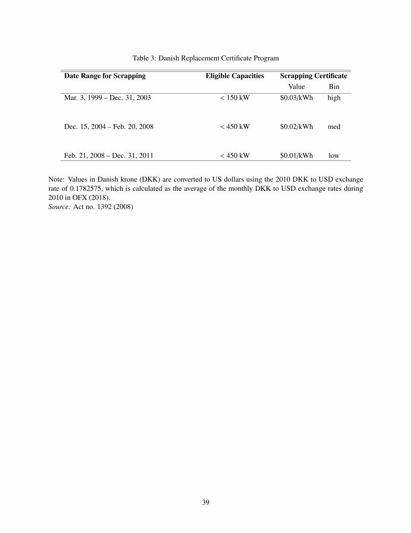
Table 3: Danish Replacement Certificate Program

Date Range for Scrapping Eligible Capacities Scrapping CertificateValue Bin

Mar. 3, 1999 – Dec. 31, 2003 < 150 kW $0.03/kWh high

Dec. 15, 2004 – Feb. 20, 2008 < 450 kW $0.02/kWh med

Feb. 21, 2008 – Dec. 31, 2011 < 450 kW $0.01/kWh low

Note: Values in Danish krone (DKK) are converted to US dollars using the 2010 DKK to USD exchangerate of 0.1782575, which is calculated as the average of the monthly DKK to USD exchange rates during2010 in OFX (2018).Source: Act no. 1392 (2008)

39

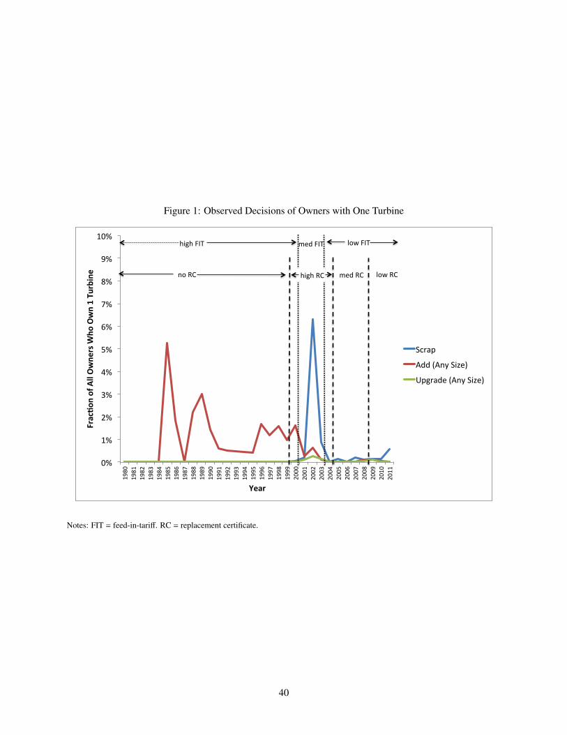
Figure 1: Observed Decisions of Owners with One Turbine

0%  

1%  

2%  

3%  

4%  

5%  

6%  

7%  

8%  

9%  

10%  

1980  

1981  

1982  

1983  

1984  

1985  

1986  

1987  

1988  

1989  

1990  

1991  

1992  

1993  

1994  

1995  

1996  

1997  

1998  

1999  

2000  

2001  

2002  

2003  

2004  

2005  

2006  

2007  

2008  

2009  

2010  

2011  

Frac%o

n  of  All  Owne

rs  W

ho  Own  1  Tu

rbine  

Year  

Scrap  

Add  (Any  Size)  

Upgrade  (Any  Size)  

high  FIT   med  FIT    

low  FIT    

no  RC   high  RC   med  RC   low  RC  

Notes: FIT = feed-in-tariff. RC = replacement certificate.

40

Figure 2: Observed Decisions of Owners with Two Turbines

0%  

1%  

2%  

3%  

4%  

5%  

6%  

7%  

8%  

9%  

10%  

1980  

1981  

1982  

1983  

1984  

1985  

1986  

1987  

1988  

1989  

1990  

1991  

1992  

1993  

1994  

1995  

1996  

1997  

1998  

1999  

2000  

2001  

2002  

2003  

2004  

2005  

2006  

2007  

2008  

2009  

2010  

2011  

Frac%o

n  of  All  Owne

rs  W

ho  Own  2  Tu

rbines  

Year  

Exit  

Scrap  One  Turbine  

Upgrade  (Any  Size)  

high  FIT   med  FIT    

low  FIT    

no  RC   high  RC   med  RC   low  RC  

Notes: FIT = feed-in-tariff. RC = replacement certificate.

41

Figure 3: Levelized Cost of Wind Energy

Note: This graph plots the levelized costs of wind energy used in our model. For comparison, the levelized costs of producing

electricity in Denmark from combined-cycle gas turbines and from steam turbine extraction generators are plotted as well. Values

in Danish krone (DKK) are deflated to 2010 DKK using the GDP deflator from the World Bank (World Bank, 2018) and then

converted to US dollars using the 2010 DKK to USD exchange rate of 0.1782575, which is calculated as the average of the monthly

DKK to USD exchange rates during 2010 in OFX (2018).

Sources: DEA (1999); Lantz et al. (2012); Levitt and Sørensen (2014b)

42

Figure 4: Interdependence of Scrapping, Adding, and Upgrading Decisions

 

Continue  

Add  

Scrap  (Exit)  

Owner  

Continue  

Scrap  

Exit  

1-­  turbine  world   2-­turbine  world  

Upgrade  

Owner  

Upgrade  

Table 4: Actions Available to Turbine Owners Owning One and Two Turbines

Action One-turbine world Two-turbine worldContinue (di,t = 1) x x

Add small turbine (di,t = 2) xAdd medium turbine (di,t = 3) x

Add large turbine (di,t = 4) xScrap only one turbine (di,t = 5) x

Upgrade to small turbine (di,t = 6) x xUpgrade to medium turbine (di,t = 7) x x

Upgrade to large turbine (di,t = 8) x xScrap all turbines (exit) (di,t = 9) x x

43

Table 5: Discretized Values for State Variables in Structural Model

Variable Value Range Bin Discrete ValueCapacity (kW) 0-450 small 1

451-750 medium 2>750 large 3

Turbine age 0-9 young 110-19 middle-aged 2>19 old 3

Price guaranteed by feed-in-tariff ($/kWh) 0.06 low 10.08 medium 20.11 high 3

Replacement certificate ($/kWh) 0.01 low 10.02 medium 20.03 high 3

Levelized cost of wind energy ($/MWh) 0-75 low 176-100 medium 2>100 high 3

44

Table 6: Results of Dynamic Structural Econometric Model

Parameter Coefficient in per-period payoffs on: (1) (2) (3)γI,1 cap kw1 Capacity of turbine 1 0.166*** 0.184*** 0.152

(0.036) (0.038) (0.128)γI,2 turbine age1 Age of turbine 1 -0.066 -0.059 -0.156**

(0.036) (0.038) (0.056)γI,3 orig f it1 Price guaranteed by feed-in-tariff for turbine 1 0.224*** 0.248*** 0.326*

(0.045) (0.044) (0.130)γI,4 orig lcoe1 Levelized cost of energy for turbine 1 -0.154*** -0.152*** 0.073

(0.022) (0.022) (0.068)γII,1 cap kw2 Capacity of turbine 2 0.012 -0.011 -0.131***

(0.046) (0.042) (0.032)γII,2 turbine age2 Age of turbine 2 0.037 0.064 0.213*

(0.106) (0.096) (0.087)γII,3 orig f it2 Price guaranteed by feed-in-tariff for turbine 2 0.011 -0.005 -0.180 ***

(0.052) (0.046) (0.039)γII,4 orig lcoe2 Levelized cost of energy for turbine 2 0.019 -0.003 -0.072

(0.043) (0.041) (0.048)α1 rep subsidy Replacement certificate 1.123*** 1.014*** 0.169

(0.290) (0.201) (1.032)α2 lcoet (Negative of) value of replacement certificate -0.467 -1.400* 1.781

(0.811) (0.654) (1.312)α3 lcoet (Negative of) value of replacement certificates for owners of 2 turbines -2.011*

(0.972)ρ1 constant (Negative of) cost of adding new turbine -6.148*** -5.394***

(0.835) (0.529)ρ2 constant (Negative of) cost of upgrading -9.068*** -8.678***

(2.046) (1.572)τ1 constant Scrap value from exiting -2.286 0.033

(2.407) (1.358)τ2 cap kw1 Scrap value of turbine 1 0.103

(1.378)τ3 cap kw2 Scrap value of turbine 2 -1.439***

(0.328)

Log likelihood -1,649.7 -1,663.7 -2,611.3

Number of observations 40,636 40,636 40,636Number of turbines 6,410 6,410 6,410Notes: Standard errors are in parentheses. Significance codes: *** p<0.001, ** p<0.01, * p<0.05.

45

Table 7: Simulated Declining Feed-in-Tariff Policy

Turbine Age Feed-in-Tariff

0 to 8 years $0.11/kWh price guarantee

9 to 16 years $0.08/kWh price guarantee

>16 years $0.06/kWh maximum price guarantee(Feed-in-tariff up to $0.02/kWh)

46

Table 8: Results of Simulations of Counterfactual Policy Scenarios, 1980-2011

Both Policiesin Place

No ReplacementCertificate

DecliningFeed-In-Tariff

NoFeed-In-Tariff

No ReplacementCertificate + NoFeed-In-Tariff

Discounted wind producer payoffs (% of actual) 100 34.2 38.4 5.03 4.05(0.51) (0.52) (0.21) (0.17)

Number of turbines scrapped 214 2,342.6 2,333.7 2,350.8 2,350.6(8.21) (8.59) (6.43) (5.81)

Number of turbines upgraded 13 1.63 1.85 0.75 0.77(1.32) (1.24) (0.83) (0.85)

Number of turbines added 129 31.55 30.84 16.77 16.98(5.88) (5.77) (4.20) (3.71)

Number of turbines scrapped by owners of 1 turbine 180 2,296.7 2,288.7 2,325.9 2,325.7(7.08) (7.74) (4.85) (4.57)

Number of turbines scrapped by owners of 2 turbines 34 45.96 44.96 24.93 24.91(9.12) (9.07) (6.56) (6.01)

Average age of turbines scrapped 16 2.92 3.00 2.10 2.11(0.04) (0.04) (0.03) (0.03)

Number of replacement certificates issued 213 NA 101.09 66.95 NA(8.46) (7.39)

Average age of turbines in 2011 13 5.03 4.99 2.00 2.00(0.44) (0.37) (0.32) (0.33)

Number of small turbines in 2011 423 3.52 2.38 1.56 2.06(1.34) (1.10) (0.70) (0.83)

Number of medium turbines in 2011 1291 17.71 16.59 1.78 1.79(4.27) (4.05) (1.24) (1.38)

Number of large turbines in 2011 472 61.93 70.67 50.50 49.68(3.97) (5.16) (2.88) (2.94)

Notes: The table reports, for each policy scenario, the means and standard deviations over 100 simulations. Standard deviations are in parentheses. Discountedwind producer payoffs are defined as the present discounted value of the entire stream of payoffs over the period 1980-2011 for each turbine owner, summedover all owners of two or fewer turbines.

47

Figure 5: Evolution of Wind Industry Under Different Policy Scenarios

0

200

400

600

800

1000

1200

1400

1979 1981 1983 1985 1987 1989 1991 1993 1995 1997 1999 2001 2003 2005 2007 2009 2011

Num

bero

fTurbine

s

Year

BothPoliciesinPlace

<450kW

450-750kW

>750kW

0

200

400

600

800

1000

1200

1400

1979 1981 1983 1985 1987 1989 1991 1993 1995 1997 1999 2001 2003 2005 2007 2009 2011

Num

bero

fTurbine

s

Year

NoReplacementCer9ficate

<450kW

450-750kW

>750kW

0

200

400

600

800

1000

1200

1400

1979 1981 1983 1985 1987 1989 1991 1993 1995 1997 1999 2001 2003 2005 2007 2009 2011

Num

bero

fTurbine

s

Year

DecliningFeed-in-Tariff

<450kW

450-750kW

>750kW

0

200

400

600

800

1000

1200

1400

1979 1981 1983 1985 1987 1989 1991 1993 1995 1997 1999 2001 2003 2005 2007 2009 2011

Num

bero

fTurbine

s

Year

NoFeed-in-Tariff

<450kW

450-750kW

>750kW

0

200

400

600

800

1000

1200

1400

1979 1981 1983 1985 1987 1989 1991 1993 1995 1997 1999 2001 2003 2005 2007 2009 2011

Num

bero

fTurbine

s

Year

NoReplacementCer9ficate+NoFeed-in-Tariff

<450kW

450-750kW

>750kW

48

Table 9: Back-of-the-Envelope Estimates of Benefits, Costs, Cost-Effectiveness, and Efficiency of Various Wind Policies, 1980-2011

ReplacementCertificate

DecliningFeed-In-Tariff

Feed-In-TariffReplacementCertificate +

Feed-In-Tariff

BenefitsPercentage point increase in discounted wind producer payoffs 65.8 33.37 94.97 95.95Total avoided carbon emissions (million tonnes CO2) 52.5 5.8 57.4 57.4

CostsTotal cost to Danish government (million US $) 1.84 to 114.12 1,114 3,547 3,549 to 3,661

Cost-EffectivenessCost per percentage point increase in discounted wind producer payoffs (million US $) 0.028 to 1.73 33.41 37.34 36.99 to 38.16Cost per million tonne CO2 avoided (million US $) 0.035 to 2.17 192.16 61.80 61.84 to 63.80

EfficiencyMinimum threshold average discounted payoffs per wind producer (thousand US $) needed in absence of any policy in order for policy to be ...... Efficient 2.74 52.71 58.97 60.25... Socially efficient when social cost of carbon is $21 US dollars per ton of CO2 -23.72 46.95 38.93 40.41... Socially efficient when social cost of carbon is $50 US dollars per ton of CO2 -60.25 38.99 11.26 13.02

Notes: Benefits and costs are calculated over the 32-year period from 1980 to 2011 for owners of two or fewer turbines (who constitute the vast majority of turbine owners inthe Danish wind industry during this time period). Discounted wind producer payoffs are defined as the present discounted value of the entire stream of payoffs over the period1980-2011 for each turbine owner, summed over all owners of two or fewer turbines.

49

Appendix A. Details of Dynamic Structural Econometric Model

In this Appendix, we explain and derive the choice probabilities in Equation (9) in more detail.

Substituting the conditional independence assumption in Equation (8) into the value functions in Equa-

tions (6) and (7) yields:

V I (xi,t, εi,t ; θ)

= max

πI,c(xi,t ; θ) + ε I,ci,t + β

∫V I(xi,t+1)dPr

(xi,t+1 | xi,t, di,t = 1, θ

),

πI,a(xi,t ; θ) + ε I,ai,t (di,t) + β

∫V II(xi,t+1)dPr

(xi,t+1 | xi,t, di,t ∈ {2, 3, 4}, θ

),

πI,u(xi,t ; θ) + ε I,ui,t (di,t) + β

∫V I(xi,t+1)dPr

(xi,t+1 | xi,t, di,t ∈ {6, 7, 8}, θ

),

πI,e(xi,t ; θ) + ε I,ei,t

(A.1)

for owners of one turbine, and:

V II (xi,t, εi,t ; θ)

= max

πII,c(xi,t ; θ) + ε II,ci,t + β

∫V II(xi,t+1)dPr

(xi,t+1 | xi,t, di,t = 1, θ

),

πII,s(xi,t ; θ) + ε II,si,t + β

∫V I(xi,t+1)dPr

(xi,t+1 | xi,t, di,t = 5, θ

),

πII,u(xi,t ; θ) + ε II,ui,t (di,t) + β

∫V II(xi,t+1)dPr

(xi,t+1 | xi,t, di,t ∈ {6, 7, 8}, θ

),

πII,e(xi,t ; θ) + ε II,ei,t

(A.2)

for owners of two turbines, where the ex ante value functions V j(·) are given by:

V j(xi,t+1) =

∫V j(xi,t+1, εi,t+1; θ)dPr(εi,t+1 | θ) = Eε

[V j(xi,t+1, εi,t+1; θ)

]for j = I, II. (A.3)

Making the assumption that each shock in εi,t is i.i.d. extreme value (type 1) across owners i, actions di,t

and time t, we can then write the expressions for the ex ante value functions V j(xt) as:

V I(xi,t) = ln

∑d

exp(δI,d

(xi,t, V‡

)) (A.4)

and:

50

V II(xi,t) = ln

∑d

exp(δII,d

(xi,t, V‡

)) , (A.5)

where:

δ j,d(xi,t, V‡

)= π j,d + β

∫V‡(xi,t+1)dPr

(xi,t+1 | xi,t, d, θ

)for j = I, II, (A.6)

and where the ex ante value function V‡ next period used to calculate the continuation value is either the ex

ante value function V I(xi,t+1) for owners of one turbine next period or the ex ante value function V II(xi,t+1)

for owners of two turbines next period, depending upon the world that an owner is in this period and the

action taken this period (similar to Equations (A.1) and (A.2)).

The probability of a given action conditional on the realization of a particular combination of state

variables is given by the following choice probabilities:

Pr(di,t = d | xi,t, θ

)=

exp(δ j,d

(xi,t, V‡

))∑

d exp(δ j,d

(xi,t, V‡

)) for j = I, II, (A.7)

which are a function of the ex ante value functions V‡ for ‡ = I, II.

51