wind turbine modeling for computational fluid dynamics
TRANSCRIPT

Wind Turbine Modeling for Computational Fluid Dynamics December 2010 mdash December 2012 LA Martinez Tossas and S Leonardi University of Puerto Rico Mayaguez Puerto Rico
NREL Technical Monitor Pat Moriarty
NREL is a national laboratory of the US Department of Energy Office of Energy Efficiency amp Renewable Energy Operated by the Alliance for Sustainable Energy LLC This report is available at no cost from the National Renewable Energy Laboratory (NREL) at wwwnrelgovpublications
Subcontract Report NRELSR-5000-55054 July 2013
Contract No DE-AC36-08GO28308
National Renewable Energy Laboratory 15013 Denver West Parkway Golden CO 80401 303-275-3000 bull wwwnrelgov
Wind Turbine Modeling for Computational Fluid Dynamics December 2010 mdash December 2012 LA Martinez Tossas and S Leonardi University of Puerto Rico Mayaguez Puerto Rico
NREL Technical Monitor Pat Moriarty Prepared under Subcontract No AFC-1-11305-01
NREL is a national laboratory of the US Department of Energy Office of Energy Efficiency amp Renewable Energy Operated by the Alliance for Sustainable Energy LLC This report is available at no cost from the National Renewable Energy Laboratory (NREL) at wwwnrelgovpublications
Subcontract Report NRELSR-5000-55054 July 2013
Contract No DE-AC36-08GO28308
NOTICE
This report was prepared as an account of work sponsored by an agency of the United States government Neither the United States government nor any agency thereof nor any of their employees makes any warranty express or implied or assumes any legal liability or responsibility for the accuracy completeness or usefulness of any information apparatus product or process disclosed or represents that its use would not infringe privately owned rights Reference herein to any specific commercial product process or service by trade name trademark manufacturer or otherwise does not necessarily constitute or imply its endorsement recommendation or favoring by the United States government or any agency thereof The views and opinions of authors expressed herein do not necessarily state or reflect those of the United States government or any agency thereof
This report is available at no cost from the National Renewable Energy Laboratory (NREL) at wwwnrelgovpublications
Available electronically at httpwwwostigovbridge
Available for a processing fee to US Department of Energy and its contractors in paper from
US Department of Energy Office of Scientific and Technical Information PO Box 62 Oak Ridge TN 37831-0062 phone 8655768401 fax 8655765728 email mailtoreportsadonisostigov
Available for sale to the public in paper from
US Department of Commerce National Technical Information Service 5285 Port Royal Road Springfield VA 22161 phone 8005536847 fax 7036056900 email ordersntisfedworldgov online ordering httpwwwntisgovhelpordermethodsaspx
Cover Photos (left to right) photo by Pat Corkery NREL 16416 photo from SunEdison NREL 17423 photo by Pat Corkery NREL 16560 photo by Dennis Schroeder NREL 17613 photo by Dean Armstrong NREL 17436 photo by Pat Corkery NREL 17721
Printed on paper containing at least 50 wastepaper including 10 post consumer waste
Abstract
With the shortage of fossil fuels and the increase of environmental awareness wind energy is becoming more imporshytant than ever As the market for wind energy grows wind turbines and wind farms are becoming larger But there is still more to learn about this technology For example current utility-scale turbines extend a significant distance into the atmospheric boundary layer Therefore the interaction between the atmospheric boundary layer and the turbines and their wakes needs to be better understood The turbulent wakes of upstream turbines affect the flow field of the turbines behind them thus decreasing power production and increasing mechanical loading With greater knowledge of this type of flow wind farm developers could plan better-performing less maintenance-intensive wind farms Simshyulating this flow using computational fluid dynamics (CFD) is one important way to gain a better understanding of wind farm flows In this study we compare the performance of actuator disk and actuator line models in producing wind turbine wakes and the wake-turbine interaction between multiple turbines We also examine parameters that affect the performance of these models such as grid resolution the use of a tip-loss correction and the way in which the turbine force is projected onto the flow field We see that as the grid is coarsened the predicted power decreases As the width of the Gaussian body force projection function is increased the predicted power is increased The acshytuator disk and actuator line models produce similar wake profiles and predict power within 1 of one another when subject to uniform inflow The actuator line model is able to capture flow structures near the blades such as root and tip vortices which the actuator disk does not capture but in the far wake they look similar The actuator line model was validated using the wind tunnel experiment conducted at the Norwegian University of Science and Technolshyogy Trondheim Agreement between the model and the experiments was obtained with the maximum percentage difference in power coefficients of 25 and 40 for thrust coefficient The actuator line and actuator disk models were compared when running large-scale wind farm simulations Normalized power was similar for both models but dimensional power differed from 1 to 17 The actuator disk model was able to run approximately three times faster though This work shows that actuator models for wind turbine aerodynamics are a viable alternative to using full blade-resolving simulations However care must be taken to use the proper grid resolution and force projection to the CFD grid to obtain accurate predictions of aerodynamic forces and hence power More work is needed to determine the best method of body force projection onto the CFD grid
iii
This report is available at no cost from the National Renewable Energy Laboratory at wwwnrelgovpublications
Abbreviations and Nomenclature
ABL Atmospheric boundary layer ADM Actuator disk model ALM Actuator line model ASM Actuator surface model BEM Blade Element Momentum CFD Computational fluid dynamics DNS Direct numerical simulation LES Large eddy simulation N-S Navier-Stokes equations RANS Reynolds-averaged Navier-Stokes SGS Subgrid-scale
CD Drag coefficient CL Lift coefficient CP Power coefficient CT Thrust coefficient p Pressure t Time U Velocity Uinfin Free stream velocity
λ Tip speed ratio νSGS Subgrid-scale viscosity ρ Density σ Solidity factor τSGS Subgrid-scale stress
iv
This report is available at no cost from the National Renewable Energy Laboratory at wwwnrelgovpublications
Table of Contents
1 Literature Review 1 11 Introduction 1 12 Basics of Wind Turbine Aerodynamics 1 13 Wind Turbine Computational Fluid Dynamics 2 14 Atmospheric Boundary Layer Simulations 3 15 Actuator Disc Model (ADM) 4 16 Actuator Line Model (ALM) 6 17 Actuator Surface Model (ASM) 7 18 Comparison Between ADM and ALM 8 19 Conclusions 8
2 Actuator Turbine Model Implementation 9 21 Actuator Line Model 9 22 Actuator Disk Model 10 23 Numerical Method 12
3 Actuator Disk and Actuator Line Models in Uniform Nonturbulent Inflow 14 31 Five Megawatt Reference Turbine 14 32 Actuator Line Model 15 33 Actuator Disk Model 15 34 Actuator Points 16 35 Tip Loss Correction 16 36 Time-step 17 37 Comparison 18 38 The ε Parameter 28
4 Wind Tunnel Simulations 31 41 Turbine Model 31 42 Mesh 31 43 Results 31
5 Wind Farm Simulation 36 51 Introduction 36 52 Results 36
6 Conclusion and Future Work 46
Bibliography 47
(Unless otherwise noted all figurestables were created by Luis A Martiacutenez)
v
This report is available at no cost from the National Renewable Energy Laboratory at wwwnrelgovpublications
List of Tables
Table 1 Percentage difference between the ADM ALM and BEM theory in terms of power production A Richardson extrapolation is used to approximate the converged solution for the ALM and ADM 21
List of Figures
Figure 1 A schematic of an actuator line turbine model 10
Figure 2 Actuator line model (left) and actuator disk model (right) simulations where the blue isosurface is of the second invariant of the velocity-gradient tensor The contours are of streamwise velocity 11
Figure 3 Plane onto which the velocity vector is projected 11
Figure 4 A schematic of an actuator disk turbine model 12
Figure 5 Domain and mesh that has a turbinewake-local resolution of 42 m The turbine is placed in the center of the domain 14
Figure 6 Power output as a function of grid resolution for different ε values 16
Figure 7 Angle of attack as a function of blade length for the ALM 17
Figure 8 Axial velocity as a function of blade length for the ALM 18
Figure 9 Mean velocity in the cross-stream direction that is 1 diameter behind the turbine rotor are shown as predicted by the ALM (left column) and ADM (right column) Each row shows plots that are the reshysult of using different values of the body force projection width (ε) 19
Figure 10 Mean velocity in the cross-stream direction that is 4 diameters behind the turbine rotor are shown as predicted by the ALM (left column) and ADM (right column) Each row shows plots that are the result of using different values of the body force projection width (ε) 20
Figure 11 Mean velocity (ms) contours in a plane through the turbine hub are shown as predicted by the ALM (left column) and ADM (right column) with a mesh resolution of Δx = 42 m Each row shows contours that are the result of using different values of the body force projection width (ε) 21
Figure 12 Vorticity magnitude (1s) contours in a plane through the turbine hub are shown as predicted by the ALM (left column) and ADM (right column) with a mesh resolution of Δx = 42 m Each row shows contours that are the result of using different values of the body force projection width (ε) 22
Figure 13 Mean velocity (ms) contours in a plane through the turbine hub are shown as predicted by the ALM (left column) and ADM (right column) with a mesh resolution of Δx = 21 m Each row shows contours that are the result of using different values of the body force projection width (ε) 23
Figure 14 Vorticity magnitude (1s) contours in a plane through the turbine hub are shown as predicted by the ALM (left column) and ADM (right column) with a mesh resolution of Δx = 21 m Each row shows contours that are the result of using different values of the body force projection width (ε) 24
vi
This report is available at no cost from the National Renewable Energy Laboratory at wwwnrelgovpublications
Figure 15 Mean velocity (ms) contours in a plane through the turbine hub are shown as predicted by the ALM (left column) and ADM (right column) with a mesh resolution of Δx = 105 m Each row shows contours that are the result of using different values of the body force projection width (ε) 25
Figure 16 Vorticity magnitude (1s) contours in a plane through the turbine hub are shown as predicted by the ALM (left column) and ADM (right column) with a mesh resolution of Δx = 105 m Each row shows contours that are the result of using different values of the body force projection width (ε) 26
Figure 17 Power output for the ALM as a function of actuator point resolution along the blade with ε = 84 and a grid resolution of 21 m 27
Figure 18 Power output as a function of grid resolution for ε = 84 m with and without a tip- and root-loss correction for the ALM 27
Figure 19 Power output as a function of time-step for ε = 84 m 28
Figure 20 Mean velocity (ms) and vorticity magnitude (1s) contours in a plane through the turbine hub for ε = 84 m are shown Each row shows contours that are the result of using different time-step values 29
Figure 21 Power and thrust coefficients as a function of tip speed ratio 32
Figure 22 Mean velocity profiles behind the rotor 33
Figure 23 Mean velocity profiles one and three diameters behind the rotor 34
Figure 24 Q-criterion (1s2) rendering showing the structure of the wake for different tip speed ratios 35
Figure 25 Wind farm layout (left) and computational domain (right) Illustration by Matthew J Churchshyfield NREL 37
macrbine in the row Average over one year of field data is shown for rows B-D 39
Figure 30 Mean streamwise velocity profiles at hub height along rows C and E at various horizontal loca-
Figure 31 Mean velocity in the cross stream direction at one-fourth diameter behind the rotor for turbines in
Figure 32 Mean velocity in the cross stream direction at one-half diameter behind the rotor for turbines in
Figure 33 Mean velocity in the cross stream direction at three-fourths diameter behind the rotor for turbines
Figure 26 Ten minute average power produced by each turbine Pi normalized by the power of the first turshy
Figure 27 Power produced by each turbine 40
Figure 28 Mean velocity (ms) contours at hub height for ADM (left) and ALM (right) 41
Figure 29 Mean velocity difference (ms) between ALM and ADM (ALM-ADM) 41
tions outboard of hub ranging from hub to blade tip 42
row D 42
row D 43
in row D 43
Figure 34 Mean velocity in the cross stream direction at 1 diameter behind the rotor for turbines in row D 44
Figure 35 Mean velocity in the cross stream direction at 3 diameters behind the rotor for turbines in row D 44
Figure 36 Mean velocity in the cross stream direction at 4 diameters behind the rotor for turbines in row D 45
vii
This report is available at no cost from the National Renewable Energy Laboratory at wwwnrelgovpublications
1 Literature Review
11 Introduction
With the shortage of fossil fuels and the increase of environmental awareness renewable energy is becoming more important than ever As the market for wind energy grows wind turbines and wind farms are growing as well Curshyrent utility-scale wind turbines extend to a significant distance into the atmospheric boundary layer (ABL) with rotor diameters of up to 120 meters (m) and 5 megawatts (MW) installed power [1] To design and control superior performing less maintenance-intensive wind farms the interaction between the ABL the turbines and their wakes needs to be better understood
In the past years wind turbine aerodynamics research has focused on acquiring high-quality experimental data and solving the incompressible Navier-Stokes equations for individual and clustered wind turbines Often actuator models are used to reduce grid requirements and simplify the problem Actuator models are the subject of this thesis The actuator disk model (ADM) represents the wind turbines as disks that impose body forces on the flow field depending on the fluid velocities Several variations of the model exist with some models taking only the axial direction of the imposed force into account and others taking only the axial and tangential forces into account The actuator line model (ALM) represents the blades as a set of points along each blade axis that rotate in time Each point defines a discrete section of the blade with its respective airfoil characteristics The lift and drag forces on the blades are calculated based on the local velocities at each point
12 Basics of Wind Turbine Aerodynamics
Wind turbines generate power by extracting kinetic energy from the wind The following analysis is based on One-dimensional Momentum Theory The air that passes through the turbine is contained within a stream tube As the power is extracted the wind expands thus increasing the cross-sectional area of the stream tube The energy extractshying device for this simple model is called an actuator disc By definition the mass of air passing through the stream tube is conserved The air velocity at the disc is related to the free stream velocity by means of the induction factor
Ud = Uinfin(1 minus a) (11)
where
Ud is the velocity at the disc
Uinfin is the free stream velocity
a is the induction factor
The momentum theory applied to a one-dimensional stream shows that power extracted from the wind is given by
Cp = P
= 4a(1 minus a)2 (12)1 ρUinfin
3A2
where
P is power
ρ is density
A is the area of the disc
The power coefficient Cp is defined as the ratio of power extracted to the available power in the mean flow Taking the derivative of Cp with respect to a allows us to find the maximum value of the function This results in an inducshytion factor of a = 13 and a maximum power coefficient of Cp = 1627 = 593 which is known as the Betz limit [2]
1
This report is available at no cost from the National Renewable Energy Laboratory at wwwnrelgovpublications
Angular momentum theory which takes into account the rotation of the wake can be used to obtain the same result [3] The thrust coefficient is another important parameter and is defined as
T = = 4a(1 minus a) (13)CT 1
ρUinfin2A2
where
T is thrust
As the wind passes through the rotor an aerodynamic thrust and torque are produced in the blades which are used then to produce power The air experiences an equal and opposite force The increase in kinetic energy of the air due to the force exerted by the blades is compensated by a decrease in pressure The circulation generated at the blades generates root and tip vortices These vortices convect downstream with the local flow velocity The vortex cylinder theory takes into account the spin of the wake yielding a lower power coefficient The vortex theory even though it does not account for wake expansion produces results that agree with the momentum theory
Blade-element momentum (BEM) theory assumes that the forces on the blade sections may be calculated from two-dimensional (2D) airfoil data The airfoil lift and drag coefficients are functions of the angle of attack Wind velocity is a combination of the velocity of the wind which accounts for axial and tangential induction and the rotation of the rotor BEM momentum theory states that the force exerted at each blade element is responsible for the change of momentum in the air that passes through the annulus which is swept by the element [2] BEM theory yields results for the power coefficient as a function of tip speed ratio
For heavily loaded turbines the momentum theory has to be modified because of the creation of a turbulent wake This causes a mixing process between the wake and the free stream This mixing process re-energizes the lower energy air that has gone through the rotor
These basic concepts are used to develop models and techniques to simulate wind turbines inside numerical codes Simulations provide results not only for the parameters affecting the turbines such as thrust and torque but also the properties of the wake formed behind the turbine
13 Wind Turbine Computational Fluid Dynamics
In past years wind turbine computational fluid dynamics (CFD) have been focused on solving the incompressible Navier-Stokes equations [4] The flow in wind turbines is incompressible with velocities ranging from 5 to 25 meters (m) seconds (s) Compressibility effects are only present at the tip because of the high velocities caused by rotation Mach number at the tip is still fairly low (M le 025) so it is reasonable to assume that the flow is incompressible even if resolving the blades Thus the incompressible Navier-Stokes equations
nabla middot u = 0 (14)
part u 1 +(u middot nabla)u = minus nablap + νnabla
2u (15)part t ρ
are suitable for wind turbine modeling
When dealing with ABL flows the Boussinesq approximation is typically used for buoyancy effects and an equation for temperature has to be solved The Coriolis effect may be present when dealing with large wind turbines and wind farms For ABL flows the largest scales are on the order of 1 kilometer (km) while the smallest scales are on the order of 1 mm This disparity of scales makes the option of using direct numerical simulations (DNS) not feasible because of the computational resources required Researches have adopted Reynolds-averaged Navier-Stokes (RANS) methods to solve the mean flow The RANS equations
part u 1 -u+(u middot nabla)u = minus nablap + νnabla2uminus nabla middot (u -) (16)
part t ρ
2
This report is available at no cost from the National Renewable Energy Laboratory at wwwnrelgovpublications
are used where over bar denotes Reynolds decomposition u = u + u -
and u-u- is the Reynolds stress tensor which is then modeled in terms of the mean flow quantities
Researchers in the wind energy wake community have adopted large eddy simulations (LES) in recent years The flow over wind turbines is highly unsteady and with the RANS equations these unsteady features are lost due to averaging A better approach is to use LES in which the flow dependence in time is resolved LES calculates the larger eddies while smaller eddies are modeled The filtered incompressible Navier-Stokes equations used are
part u 1 +(u middot nabla)u = minus nablap + νnabla
2uminus nabla middot (uuu minus uu) (17)part t ρ
where
the term (uuu minus uu) is often modeled by
τSGS = (uuu minus uu) = minusνSGS(nablau+(nablau)T ) (18)
and νSGS is the subgrid-scale (SGS) viscosity and is modeled using several subgrid-scale models The filtering u + u --operation was applied at u = ˜
In past years RANS and LES have been used to simulate wind turbine flow However researchers are increasingly using LES because of its ability to better predict the ABL and the wake behind wind turbines
14 Atmospheric Boundary Layer Simulations
The principal factors that affect the behavior of the ABL are the geostrophic wind the surface roughness and terrain the Coriolis effects and thermal stratification Thermal stratification is categorized as stable unstable and neutral Unstable stratification occurs when there is significant surface heating causing the warmer air near the surface to rise When a volume of air rises the pressure exerted upon it decreases and it expands and cools nearly adiabatically With respect to elevation if the rate of cooling of the volume of air does not equal or exceed the lapse rate of the ABL (the vertical gradient of temperature) it will keep rising resulting in enhanced vertical mixing and a thicker ABL If the ground is cold the vertical motion of the air will be suppressed thus giving rise to stable stratification Neutral stability occurs as the wind reaches thermal equilibrium with its surroundings as it rises
To mimic the ABL for wind turbine wake simulations the boundary conditions of the flow need to be prescribed Different boundary conditions are used to simulate ABL scenarios such as the sheared velocity profile the anisotropy of the turbulence and the instationary nature of the flow The bottom surface is usually described as a no-slip boundshyary condition or a wall function to account for roughness At the upper boundary stress and flux-free conditions are usually employed In the streamwise direction periodicity is usually employed to simulate infinite wind farms or as a precursor to generate the ABL turbulence Periodicity conditions are convenient from a numerical point of view due to the application of fast solvers
Porteacute-Agel et al [5] performed an LES of the ABL with wind turbines The SGS stresses and heat flux were modshyeled using tuning-free scale-dependent Lagrangian dynamic models They compared the results with experimental data from a wind tunnel at the St Anthony Falls Laboratory using miniature wind turbines The LES code solved the filtered continuity equation the filtered momentum equations (in rotational form) and the filtered temperature transport equation Buoyancy effects were taken into account by means of the Boussinesq approximation The deshyviatoric part of the SGS model was calculated using an eddy viscosity model while the SGS heat flux model used an eddy-diffusivity model The scale-dependent Lagrangian dynamic SGS models implemented take into account the anisotropy of the flow by dynamically adjusting the Smagorinsky coefficient The surface shear and heat flux at the bottom were calculated by means of the Monin-Obukhov theory using instantaneous (filtered) fields The upper boundary condition was a stress- and flux-free condition
Calaf et al [6] used a pseudo-spectral code to model the ABL This study focused on investigating a fully develshyoped wind-turbine-array boundary layer Two different LES codes were used One method used the skew-symmetric
3
This report is available at no cost from the National Renewable Energy Laboratory at wwwnrelgovpublications
form of the Navier-Stokes equations with a pseudo-spectral discretization with periodic boundary conditions in the horizontal direction and centered second-order finite differencing in the vertical direction The second code used a pseudo-spectral discretization in the horizontal direction but fourth order energy-conservative finite differshyence discretization in the vertical direction Time integration was done using the fourth order Runge-Kutta scheme The standard Smagorinsky sub-grid model was used in both cases The roughness height was approximated using Lettaursquos formula The flow used was fully developed and driven by means of an imposed pressure gradient The turbulent kinetic energy vertical fluxes were of the same order of magnitude as the power extracted by the wind turshybines The study focused on equivalent roughness models of wind farms and proposed that the modified Frandsen formula to calculate the roughness height of the wind farm
In their study Troldborg et al [7] used the three-dimensional (3-D) flow solver EllipSys3D developed by Mikkelsen and Soslashrensen The code solved the incompressible Navier-Stokes equations in general curvilinear coordinates using a block structured finite-volume approach The SGS viscocity was modeled by means of the vorticity-based mixed-scale model by Ta Phuoc et al [8] The pressure was solved by means of the Pressure Implicit with Splitting of Operators algorithm
When doing large eddy simulation (LES) of the ABL the spatial resolution is such that it does not fully resolve the blade geometry of a wind turbine It is impossible to fully resolve the flow in the ABL and around a wind turbine at the same time especially considering the computational resources that are currently available This is the main reason to develop wind turbine actuator models that can simulate wind turbines without having to resolve the full geometry
15 Actuator Disc Model (ADM)
The ADM simulates the turbine as a disc within the flow that imposes forces on the fluid Many versions of the ADM exist Some apply thrust and tangential forces while others only apply thrust Many researchers have adopted the ADM for simulating wind turbines Even though the ADM may simulate the turbines and their wakes it does not create the tip vortices that are carried onto the wake [9]
Porteacute-Agel et al [5] compared two different versions of the ADM the ADM that applies both thrust and tangential force and the one that applies only thrust The actuator disk model with no tangential force is based on the momenshytum theory of propellers The actuator disk force is distributed uniformly over the circular disc The force exerted on the disc is given by
1 2T = ρ u0ACT (19)2
where
T is the thrust force
ρ is the density 2u0 is the unperturbed resolved velocity of the axial incident flow in the center of the rotor disk
A is the rotor swept area
CT is the thrust coefficient
This model presents a one-dimensional approximation of the thrust force and does not take into account the rotation in the flow produced by the blades It also does not seem to take into account radial variation of T
The ADM with tangential force is implemented by integrating the lift and drag by the blades over the spatial and temporal resolution used in the LES The force implemented by the actuator disc model (vectors are in bold) is given by
dF 1 Bcf2D = = ρV 2 (CLeL +CDeD) (110)rel dA 2 2πr
4
This report is available at no cost from the National Renewable Energy Laboratory at wwwnrelgovpublications
where
B is the number of blades
Vrel is the local velocity
CL is the lift coefficient
CD is the drag coefficient
c is the chord length
and eL and eD are the unit vectors in the direction of lift and drag respectively
Calaf et al [6] used the ADM in their study The wind turbines were modeled by means of the acirc AIAIJdrag diskacirc concept The momentum equation had an extra term for the thrust force of the turbines The velocity used for the model was averaged over the disk region The total force was distributed among all the grid points that fell into the wind turbine disk region The grid spacing was uniform in all directions
The wind turbine model used the classic model for one directional force
T = minus 1
ρCTU2 π D2 (111)infin2 4
where
CT is the thrust coefficient
and Uinfin is the upstream undisturbed reference velocity
The values for the thrust coefficients used are CT = 75 and the induction factor a = 14 which can be found in existing wind turbines The force is calculated by averaging the velocity throughout the area swept by the actuator disk The force is distributed on each cell and depends on the frontal area of the cell which coincides with the area of the disc The forces at each cell are distributed among surrounding cells by means of a Gaussian convolution filter
In their work Ammara et al [10] used the ADM and solved the Navier-Stokes equation with a control-volume finite element method Axial and tangential forces were taken into account in the model as well as a tip correction factor to account for blade tip effects The calculations were compared to experimental data from the US Department of Energy MOD-0A rotor and MOD-2 cluster where an acceptable level of accuracy was obtained in terms of wake velocity predictions and wind farm performance
Jimenez et al [11] implemented the ADM into a CFD code based on a LES approach The ADM model used acshycounted only for thrust forces thus neglecting rotational effects The force imposed on the flow was
T = minusCT 1
Au02 (112)
2
where
CT is the thrust coefficient of the turbine
A is the frontal area of the cell
and u0 is the unperturbed velocity of the incident flow at the center of the disk
The velocity profile incident over the turbine agreed with the logarithmic law while the velocity value in the upper part of the domain was larger than what the law of the wall provided Discrepancies between computations and measurements in the turbulence intensity of the wakes were found in the flow direction
Masson et al [12] performed simulations using the actuator disc concept The tower was modeled in a similar manshyner as a permeable wall The model was tested using a 3D Cartesian and an axisymmetric polar solver and was
5
This report is available at no cost from the National Renewable Energy Laboratory at wwwnrelgovpublications
compared to the Tjaereborg turbine In addition the National Renewable Energy Laboratory (NREL) combined exshyperimental rotors obtaining good results Discrepancies were attributed mostly to the turbulence and dynamic stall modeling
Mikkelsen et al [13] used an actuator disk model to investigate the effects of rotor coning In the model blade element momentum was used to calculate the forces of the blades imposed on the fluid For the coned rotor the interference factors were found to change considerably with the radius of the disc It was shown that BEM theory under-predicts the blade-root shear and power coefficients by up to 7
The ADM provided reasonable overall results however there are still many things to improve For example the forces imposed on the fluid were averaged through the rotor whereas the actual forces acted only in the instantaneous location of the blades The ADM was not able to capture tip vortices which are important when studying the near wake of a wind turbine With these limitations researchers have devised other models which improve the results provided by the ADM
16 Actuator Line Model (ALM)
The ALM models the wind turbine blades as a set of blade elements along each blade axis The model uses airfoil data to calculate lift and drag at each element and applies to the flow field as body forces The ALM does not resolve the full geometry of the blades
Soslashrensen et al [14] implemented the ALM to study the dynamics of the wake and the tip vortices The body forces were calculated based on tabulated airfoil data The total force on a blade element is
= dF
= 1
ρU2 (113)f2D rel c(CLeL +CDeD)dA 2
where
CL and CD are the lift and drag coefficients
Urel is the local wind velocity
and eL and eD are the unit vectors in the direction of lift and drag respectively
The blade element forces are projected using a convolution
fε = f otimes ηε (114)
where
ηε is a regularization function
They use a Gaussian given by
ηε = 1
exp[minus(rε)2] (115)ε3π32
where
ε establishes the width of the function The model was validated by comparing power output data from the Nordtank turbine
Ivanell et al [15] used direct numerical simulations to study the wakes behind a wind turbine The turbine was repshyresented by using the actuator line model Tabulated airfoil data was then used to calculate the body forces imposed on the fluid This study paid special attention to the tip vortices The solver used a finite-volume discretization of the Navier-Stokes equations in general curvilinear coordinates The Reynolds number based on inflow velocity and rotor radius was 50000 with a mesh of about 5 million grid cells The body forces imposed on the fluid by the turbine
6
This report is available at no cost from the National Renewable Energy Laboratory at wwwnrelgovpublications
model were projected by means of a Gaussian convolution This study also used a 2D convolution on the plane orshythogonal to the actuator line The results were compared to the Tjaereborg turbine with a 10 ms wind speed and a tip speed ratio of 7 It was found that the circulation along the blades was nearly constant
Troldborg et al [7] performed large eddy simulations using the ALM with the vorticity-based mixed-scale model by Ta Phuoc The model was compared to field measurements of the Tjaereborg turbine and obtained agreement It was observed that the far wake followed an axial velocity distribution resembling a Gaussian shape The regularization parameter ε was studied by finding an optimum value where the forces were projected in such a way that the model was able to capture root and tip vortices The discrepancies in the model were attributed to the inaccuracy of the 2-D airfoil data and to the non-inclusion of the nacelle in the model
Mikkelsen et al [16] performed studies on multiple turbines using the ALM The model was tested on a row of turshybines with pitched blades The wakes interacted in a fully unsteady nonlinear manner In his PhD thesis Mikkelsen investigated the ALM in detail in a finite volume solver using pressure-velocity formulation in curvilinear coordishynates [17]
In his PhD thesis Troldborg performed a detailed study of the ALM [9] The ALM model was tested for different tip speed ratios showing different wake developments Power coefficient comparisons with measured data showed good agreement Discrepancies were attributed to inaccurate airfoil data When subjected to shear-flow the non-symmetric rotor loading caused a skewed wake development When subjected to non-sheared turbulent inflow the wake broke up quickly thereby increasing turbulence levels in the wake As the wake progressed in sheared and turbulent flow the asymmetry gradually diminished When studying three turbines in a row the turbulent case caused higher inflow velocities on the downstream turbines due to the faster wake recovery When studying two turbines in a row under the ABL that was characterized by strong shear and low-ambient turbulence the second turbine experienced tilt moment caused by the wind shear and severe yaw moments The wake of the first turbine did not break up before reaching the second one resulting in a complex inflow for the second turbine
The ALM yielded accurate results but it still had limitations Each blade-element force was the total force over that element whereas the real forces were distributed smoothly over the chord of the blade-element To distribute the blade element point force a Gaussian projection was used which eliminated numerical instabilities but did not reproduce the actual force distribution on the blades Other projections are possible though
17 Actuator Surface Model (ASM)
Another model that has been explored recently is the ASM This model calculates the forces on a 2-D airfoil as a function of the chord thus avoiding one of the major simplifications of the ALM This is done by using empirical formulas with forces as a function of the chord position Shen et al [18] investigated the ASM on a NACA0015 airfoil The model predicts accurate results using a 2 dimensional Navier-Stokes incompressible solver In a vertical axis wind turbine the model failed to accurately predict the normal and tangential forces This was improved by using the Leishman-Beddoes dynamic stall model
Dobrev et al [19] discussed the application of an actuator surface hybrid model The model uses blade-element momentum theory (BEM) in a computational fluid dynamics (CFD) solver The model was implemented using Fluent CFD package The results were compared with the NREL Phase VI experiment data and showed satisfying agreement It was noted that it is important to employ a correction for the circulation distribution near the tip region as well as the induced velocity angles
In their study Watters et al [20] conducted a more thorough investigation of the ASM Two- and three-dimensional versions of a control-volume finite element method model were used to compute inviscid flow The ASM produced accurate results when compared to the Prandtl lifting model The model was validated using the wind turbine rotor of the Technical University of Delft and obtained encouraging results The flow structures inherent to a vortical wake were well reproduced The model can be used to simulate propellers helicopters and wind turbines Furthermore integration of viscous drag in the model is a subject of interest that could be explored to help improve the model
7
This report is available at no cost from the National Renewable Energy Laboratory at wwwnrelgovpublications
The ASM is a promising approach for modeling wind turbines in CFD solvers The modelrsquos main advantage is its ability to provide a more realistic force distribution The limitation of the ASM is its dependency on an external calculation for the force distribution as a function of position within the chord of an airfoil
18 Comparison Between ADM and ALM
Porteacute-Agel et al [5] compared the ADM that calculates thrust and tangential forces (ADM-R) the ADM that imshyposes only thrust force (ADM-NR) and the ALM The ALM calculates lift and drag for discrete sections of the blade and distributes them along the blades The ALM as opposed to the ADM captures tip vortices and coherent periodic helicoidal structures in the near-wake region The turbine induced force is
dF 1 ρV 2f2D = = rel c(CLeL +CDeD) (116)
dA 2
The forces in these models are projected smoothly onto the flow field to avoid singular behavior and numerical instability The forces are projected by means of a Gaussian distribution The nacelle and tower are modeled as drag forces and include their respective drag coefficients
The numerical models were compared to experimental results from wind tunnel measures at the Saint Anthony Falls Laboratory The turbine wakes were characterized using the streamwise velocity and the streamwise turbulence intensity The ALM and the ADM-R were in agreement with the experimental data The ADM-NR yielded a poor prediction of the mean velocity distribution
The maximum turbulence intensity in the experiments was found near the top tip at a normalized distance of 3 to 5 diameters downstream The numerical models captured different turbulent intensities but the ADM-R and the ALM were in agreement with the experimental data
The ALM was implemented into an LES code for a stable boundary layer The model was able to capture blade-induced 3-D helicoidal tip vortices As stated by previous studies the results showed that wind farms create an impact on local meteorology
19 Conclusions
In the past years wind turbine aerodynamic research was focused on solving the incompressible Navier-Stokes equations Not until recently have people done real ABL simulations with turbines It is much more common for people to use a general (not ABL-specific) solver by applying stochastic turbulence at the inlet to try to simulate ABL flow Often the turbines are modeled using several actuator models thereby eliminating the need to resolve the full geometry of the blades The ADM simulates the turbines as a permeable disc in the flow field and can yield good results if tangential forces are taken into account The ALM represents the turbine blades as lines that impose body forces on the fluid thereby yielding accurate results The ASM represents the blades as 2-D actuating surfaces that impose body forces on the flow field
Future research efforts will be aimed at simulating wind farms and aeroelastic coupling between the flow field and the turbines [1] The behavior of the wake and the interaction between wakes in the ABL flow are not fully understood yet These challenges will be a motivation for researchers to achieve better modeling of wind turbine aerodynamics
8
This report is available at no cost from the National Renewable Energy Laboratory at wwwnrelgovpublications
2 Actuator Turbine Model Implementation
The actuator disk model (ADM) and actuator line model (ALM) predict blade forces depending on the local fluid velocity at each actuator element These forces are then projected onto the flow field as body forces and imposed into the Navier-Stokes equations The forces calculated in the models are point forces for individual blade sections To distribute point forces onto the surrounding volume the forces are projected by means of a Gaussian function
eefturb =
F exp[minus(rε)2] (21)
ε3π32
where
efturb is the projected body force per unit volume
eF is the force at the actuator element
ε establishes the projection width
and r is the distance from the location of the actuator element center to the point where the force is applied
The function decays to 1 of its maximum value when r = 215ε
The models calculate blade quantities such as angle of attack lift and drag by using the local velocity at each actuashytor point The local angle of attack is taken to be the angle between the chord and the local flow This assumption is made knowing that the actuator point lies within the center of the bound vortex where the effects of up- and down-wash are small Tabulated airfoil data are used to obtain the lift and drag coefficients Power output is calculated by integrating the torque created with respect to the center of the rotor and multiplying it by the rotational speed of the rotor
21 Actuator Line Model
The geometry of the wind turbine is defined in a Cartesian coordinate system The geometry of the turbine is created based on three key point locations nacelle hub and ground The nacelle point is connected to the ground point by a vertical line The hub point is connected to the nacelle point with a line defined by the turbinersquos yaw angle into the wind and the tilt angle between the horizontal plane and the nacelle axis This is the line about which the blades rotate The blades are defined as a series of points along each bladersquos axis and each point is the center of an actuator element The first blade is defined as a line parallel to the ground (x-y) plane The other blades are created by using a rotation matrix as follows ⎡ ⎤⎡ ⎤2 2ux +(1 minus ux )c uxuy(1 minus c) minus uzs uxuz(1 minus c)+ uys x0 2 2⎣ ⎦⎣uxuy(1 minus c)+ uzs uy +(1 minus uy )c uyuz(1 minus c) minus uxs y0⎦ = x1 y1 z1 (22)
2 2uxuz(1 minus c) minus uys uyuz(1 minus c)+ uxs u +(1 minus u )c z0z z
where
c = cos(θ ) and s = sin(θ )
eu = uxeex + uyeey + uzeez is the unit vector normal to the plane of rotation
θ is the angle of rotation x0 y0 and z0 are the coordinates of the point to be rotated
and x1 y1 and z1 are the coordinates of the rotated point
The blades are rotated at each time step by using the angular speed of the rotor The locations of all the points along each blade are rotated using the rotation matrix in Equation 22 Figure 1 shows a schematic of the ALM and the left side of Figure 2 is an example of the wake and vortex system it creates The figure shows a horizontal contour plane through the hub of streamwise velocity
9
This report is available at no cost from the National Renewable Energy Laboratory at wwwnrelgovpublications
The actuator line points define the location of different sections of the blades that have a specific lift and drag deshypending on their airfoil type twist angle chord length and incoming flow conditions A lift and drag resultant body force vector can be assigned to each actuator line point The body force equal and opposite to the lift and drag is imshyposed in the momentum equation The lift and drag are calculated based on the local wind speed and angle of attack
1L =
2CL(α)ρV 2cw (23)
D = 1 2
CD(α)ρV 2cw (24)
where
α is the local angle of attack with respect to the chord
CL(α) is the lift coefficient
CD(α) is the drag coefficient
ρ is the densiy
V is the local wind speed
c is the chord
and w is the width of the section
These forces are then projected onto the flow field by means of the Gaussian function shown in Equation 21
The plane where the body force vector lies is perpendicular to the actuator lines as shown in Figure 3 The planes are created by defining two new vectors x - and y - The cross product of the directional vector of the actuator line z - and the vector around which the blades rotate gives the resultant directional vector pointing in the tangential direction of rotation of the blades y - The cross product of the new vector y - and the z - vector gives the vector x - which is also used to define the plane where the forces lie The new set of vectors is updated every time step for each blade according to the rotation of the blades The velocity vector is projected onto the new plane by means of the dot product
Figure 1 A schematic of an actuator line turbine model
22 Actuator Disk Model
The ADM simulates the turbine blades as a disk inside the flow field that occupies the swept area of the blades This is done by dividing the rotor swept area into many elements The geometry of the ADM is similar to the ALM The
10
This report is available at no cost from the National Renewable Energy Laboratory at wwwnrelgovpublications
Figure 2 Actuator line model (left) and actuator disk model (right) simulations where the blue isosurshyface is of the second invariant of the velocity-gradient tensor The contours are of streamwise velocity
Figure 3 Plane onto which the velocity vector is projected
difference is that there are as many actuator lines as there are circumferential sections Each point now represents a section of the disk Figure 4 shows the schematic of an ADM where each actuator point represents an element in the disk In addition the right side of Figure 2 shows an example of the wake and vortex system created by the ADM The force at each element is scaled by a solidity factor
NABσ = (25)
Ar
11
This report is available at no cost from the National Renewable Energy Laboratory at wwwnrelgovpublications
where
N is the number of blades
AB is the area of an individual section
and Ar is the swept area of the blades
The lift and drag forces on each actuator disk element are given by
L = σ 1
CL(α)ρV 2cw (26)2
D = σ 1
CD(α)ρV 2cw (27)2
Figure 4 A schematic of an actuator disk turbine model
23 Numerical Method
To use the ADM and ALM a CFD solver is used We implemented the solver using the OpenFOAM (Open Field Operation and Manipulation) toolbox [21] The OpenFOAM package is a set of C++ libraries meant for solving partial differential equations The turbine models were implemented as C++ classes called by the solver A finite-volume approach is used to discretize the governing equations The filtered Navier-Stokes equations are solved along with the standard Smagorinsky [22] model
The large eddy simulation (LES) code solves the incompressible Navier-Stokes equations The flow around wind turbines is incompressible with velocities ranging from 5-25 meters per second (ms) The incompressible filtered Navier-Stokes equations
nabla middot u = 0 (28)
part u minus+(u middot nabla)u = minus
1 nablap+ νnabla
2uminus nabla middot τSGS + rarrf turb (29)
part t ρ
are suitable for wind turbine modeling
where
u is the filtered velocity vector
p is the filtered pressure
12
This report is available at no cost from the National Renewable Energy Laboratory at wwwnrelgovpublications
ν is the kinematic viscosity
efturb is the turbine force
nabla middot τSGS = minusνSGS(nablau+(nablau)T )
and νSGS is the subgrid-scale viscosity and is modeled using the Smagorinsky subgrid-scale model
13
This report is available at no cost from the National Renewable Energy Laboratory at wwwnrelgovpublications
3 Actuator Disk and Actuator Line Models in Uniform Nonturbulent Inflow
The accuracy of the actuator disk model (ADM) and actuator line model (ALM) in predicting aerodynamic forces torque and power production depends largely on grid resolution and the projecting function To study these paramshyeters we performed a grid resolution study The solution was compared to the results that were from the NREL-developed WT_Perf [23] code which uses blade-element momentum (BEM) theory Cases were studied with differshyent values of the parameter ε which establishes the width of the Gaussian projecting function
eefturb =
F exp[minus(rε)2] (31)
ε3π32
All the meshes were created by starting with a background grid of 168-meter (m) resolution Regions of successive refinement were introduced into the background grid to provide higher resolution around the turbine and wake Each refinement region was created by splitting cells in half in each direction within that region Three different grids were made each with a different resolution that was local to the turbine and wake Those turbinewake-local resolutions were Δx = Δy = Δz =42 m 21 m and 105 m The domain was 10 rotor diameters (D) wide in all directions with the turbine rotor placed in the geometric center of the domain The finest region extended 1 diameter upstream of the turbine and 5 diameters downstream It extended 1 diameter beyond the edge of the rotor in the other two directions Figure 5 shows the mesh for a case that has three successive local refinements for a resolution of 42 m Cases were run for four different values of the ε parameter ranging from 42 m to 105 m The ALM case with ε = 84 m was tried with and without the Glauert tip loss correction [24] Cases for the ALM that had different number of actuator elements per blade span and cases with different time-step were run with a grid resolution of 21 m and ε = 84 m
Figure 5 Domain and mesh that has a turbinewake-local resolushytion of 42 m The turbine is placed in the center of the domain
31 Five Megawatt Reference Turbine
The turbine modeled was the 5-megawatt (MW) reference turbine designed by Jonkman et al [25] This horizontal-axis upwind turbine has three blades with a rotor diameter of 126 m a hub height of 90 m a rated wind speed of 114 meters per second (ms) and 5-MW-rated power production Simulations were performed with an inflow
14
This report is available at no cost from the National Renewable Energy Laboratory at wwwnrelgovpublications
condition of 8 ms The rotational speed of the rotor was fixed at 91552 revolutions per minute giving a tip speed ratio of 755 which happens to be this turbinersquos normal Region 2 tip speed ratio We chose these conditions because they provide the optimum power coefficient of the turbine and thereby extract maximum energy from the flow This is when the wakes are strongest and the wake effects are the most important
32 Actuator Line Model
Power output predicted by the ALM is shown in Figure 6 as a function of grid resolution The power output inshycreases as the grid is refined As ε becomes larger the predicted power increases The larger the ε value the smaller the rate of change of predicted power as a function of grid resolution When ε = 42 m the difference in power predicted on the finest grid and the coarsest grid is 300 kilowatts (kW) When ε = 105 m the difference is 40 kW which is much smaller Power production is clearly more grid-dependent for smaller values of ε Simulations for ε = 21 m were run with grid resolution of Δx = 105 m and 0525 m This value of ε is limited to a minimum grid resolution of 105 m because numerical instabilities appear when ε lt 2Δx The trend is followed by showing that a smaller ε will produce less power The BEM solution for power output is 1926 MW This value falls between the finest cases with ε = 42 and 21 m
Figure 7 shows time-averaged angle of attack as a function of blade length The difference in angle of attack proshyvides different lift and drag coefficients thus predicting a different force on the blades and causing different power outputs The axial velocity at the actuator element center points is shown as a function of blade length in Figure 8 It appears that a larger ε causes less axial induction at the actuator element center points (where velocity is sampled and angle of attack is computed) and also causes more power production because the force is too smoothed out
Velocity profiles through the wake along a horizontal line 1 diameter downstream at the hub height are shown in Figure 9 For the cases of ε le 63 m and Δx = 42 m the profiles have a different shape compared to all other cases When εΔx ge 32 the resolution Δx becomes important and we can observe instabilities in the results The instabilities are greater near the outmost portion of the blades where the forces are greater We observe small differences for each resolution and as the ε parameter becomes larger these differences become even smaller A grid resolution of Δx = 21 m appearss to provide converged wake profiles for each value of ε Figure 10 shows wake profiles 4 diameters downstream The profiles for the case of ε = 42 m and Δx = 42 m are affected by the numerical instabilities near the rotor which are smoothed further downstream
Mean wind speed and vorticity magnitude contours are shown in Figure 11 through Figure 16 The simulations in Figure 11 and 12 when ε = 42 m are subject to numerical instabilities These instabilities are due to the fact that εΔx = 1 where there is the limitation that ε ge 2Δx for an oscillation-free solution The velocity in the center of the wake is greater than at larger radii This is expected because the hub and nacelle are not included in the model the difference in velocity is the effect of the blades only The blades are also not as loaded at the root as they are farther outboard so they do not decelerate the flow there as much Mean speed profiles are similar for different values of ε The main difference observed is in the middle of the wake where there is a jet A larger value of ε projects the forces further beyond the root leaving a small gap between the blades for the jet to form This leaves less space for the jet as the ε value is increased As the ε value is decreased the shear layer becomes thinner and more unstable at the rotor tip and root causing a faster transition to turbulence This effect is illustrated in Figure 14 which shows that a smaller value of ε produces more vorticity The structure of the instantaneous ALM wake is not symmetric with respect to the center of the wake because the vortical structures produced by individual blades are helical and asymmetric across the wake This asymmetry causes asymmetric roll-up of Kelvin-Helmholtz-like instabilities in the outer shear layer of the wake As the grid is refined vorticity contours show more structures that are filtered in coarser grids
33 Actuator Disk Model
Power output predicted by the ADM is shown as a function of grid resolution in Figure 6 Power output increases as the grid is refined for all cases similar to the ALM Wind speed profiles through a horizontal line that are 1 diameter
15
This report is available at no cost from the National Renewable Energy Laboratory at wwwnrelgovpublications
downstream at hub height are shown in Figure 9 For the case with Δx = 42 m and ε = 42 m the solution has numerical oscillations similar to the ALM The case with Δx = 42 m and ε = 63 m has a different shape near the edge of the wake compared to the more refined cases As in the ALM this is caused by the numerical instabilities near the tip of the blade Wake profiles shown in Figure 10 appear to converge for all resolutions except when Δx = 42 m and ε = 42 m This is due to the numerical instabilities near the rotor as in the ALM cases
Mean wind speed and vorticity contours for cases with Δx = 21 m are shown in Figures 13 and 14 Mean wind speed contours are similar to the ones for the ALM Vorticity contours show the turbulent structures near the edge of the wake that are caused by the shear layer As the value of ε becomes smaller the shear layer is stronger thus increasing the turbulence in the wake (similar to what happens in the ALM) There is no formation of tip- and rootshyvortices when using the ADM These structures are formed because the bound circulation of each blade is shed at the tips in the form of vortices A continuous disk covering the swept area of the blades does not have discrete tips on which vortices are shed The wake is symmetric with respect to the center of the wake This is due to the fact that the rotor is modeled as a continuous disk rather than as individual blades There are no asymmetric helical tip-vortices to cause asymmetric Kelvin-Helmholtz-like transition to turbulence
ALM ADM
Figure 6 Power output as a function of grid resolution for different ε values
34 Actuator Points
Power output is shown as a function of blade segment resolution with ε = 84 m in Figure 17 The actuator points are distributed uniformly along the blade The resolution of the blade is presented in terms of the grid resolution (ΔbΔx) where Δb is the width of the discrete blade section and Δx is the grid resolution The number of blade sections should be high enough to predict a smooth body force field along the blades This criterion should be the basis for establishing the blade resolution A value of ΔbΔx = 3 did not predict a smooth transition through the blade thus the solution is not reliable Values below ΔbΔx = 1 predict smoothed forces along the blade The power output appears to converge after reaching a value of ΔbΔx = 05
35 Tip Loss Correction
Figure 18 shows power output as a function of grid resolution for ε = 84 m with and without a Glauert tip- and root-loss correction [24] The use of a tip- and root-loss correction makes the lift go to zero more gradually at the
16
This report is available at no cost from the National Renewable Energy Laboratory at wwwnrelgovpublications
ε = 42 m ε = 63 m
ε = 84 m ε = 105 m
Figure 7 Angle of attack as a function of blade length for the ALM
tip and root of the blade This correction decreases the total force on the blade creating less torque which results in lower power production Figure 18 illustrates this effect showing a difference of about 90 kW between the simulashytions Since the ALM produces tip-vortices that cause losses a tip-loss correction is not necessary if the tip vortices are well resolved
36 Time-step
It is advised by researchers in the field to use a Δt which allows the tip of the blade to not advance through more than one grid cell at each time-step This condition is very restrictive because it requires a time-step smaller than what would be required by the more conventional Courant-Friedrichs-Lewy (CFL) condition Figure 19 shows power output as a function of time-step for ε = 84 m This shows a linear profile with a power variation ranging from 1 to 2 This difference is small and does not suggest that the time-step is making a big difference in the simulation Figure 20 shows mean velocity and vorticity contours for different time-steps The profiles are very similar for all cases suggesting that the time-step does not cause a significant difference The value of ε = 84 used in this simulation is large A smaller ε might produce different results because the tip vortices are more pronounced As far as ε = 84 m the time-step needs to not be limited by the tip speed
17
This report is available at no cost from the National Renewable Energy Laboratory at wwwnrelgovpublications
ε = 42 m ε = 63 m
ε = 84 m ε = 105 m
Figure 8 Axial velocity as a function of blade length for the ALM
37 Comparison
The ALM and ADM predict similar wake profiles and power output The main differences between the models are 1) the vortical structures near the rotor were captured by the ALM but not by the ADM and 2) a non-symmetric wake was observed with respect to the center-line with the ALM as opposed to the symmetric wake that was obshyserved in the ADM The ALM is able to capture vortical structures that are caused by the presence of individual blades Tip and root vortices are captured when using the ALM with a high enough grid resolution as seen in Figure 14 when ε = 42 m However the ADM does not allow these structures to form only the shear layer of the wake forms
Table 1 compares power output for the ADM ALM and BEM theory A Richardson extrapolation is used to elimishynate the leading error and predict the grid-converged power solution for the ADM and ALM The power has a similar behavior for the ADM and ALM As ε becomes smaller the power output for the ADM and ALM approaches what the BEM theory predicts Both models provide similar results but as ε becomes smaller the differences are bigger
In terms of computational costs the ALM needs to rotate the blades every time-step and thus apply forces at difshyferent finite-volume cells every time-step A search for these cells is performed every time-step The ADM points are fixed and do not rotate every time-step All the cells that lie adjacent to the disk are assigned at the beginning of the simulation thus all the finite-volume cells that have an applied force are searched for only once The ADM by
18
This report is available at no cost from the National Renewable Energy Laboratory at wwwnrelgovpublications
ALM ADM
ε = 42 m
ε = 63 m
ε = 84 m
ε = 105 m
Figure 9 Mean velocity in the cross-stream direction that is 1 diameter behind the turbine rotor are shown as predicted by the ALM (left column) and ADM (right column) Each row
shows plots that are the result of using different values of the body force projection width (ε)
19
This report is available at no cost from the National Renewable Energy Laboratory at wwwnrelgovpublications
ALM ADM
ε = 42 m
ε = 63 m
ε = 84 m
ε = 105 m
Figure 10 Mean velocity in the cross-stream direction that is 4 diameters behind the turbine rotor are shown as predicted by the ALM (left column) and ADM (right column) Each row
shows plots that are the result of using different values of the body force projection width (ε)
20
This report is available at no cost from the National Renewable Energy Laboratory at wwwnrelgovpublications
ALM ADM
ε = 42 m
ε = 63 m
ε = 84 m
ε = 105 m
Figure 11 Mean velocity (ms) contours in a plane through the turbine hub are shown as predicted by the ALM (left column) and ADM (right column) with a mesh resolution of Δx = 42 m Each row shows contours that are the result of using different values of the body force projection width (ε)
Table 1 Percentage difference between the ADM ALM and BEM theory in terms of power producshytion A Richardson extrapolation is used to approximate the converged solution for the ALM and ADM
Case Predicted Power (MW) Percentage Difference with BEM ALM ADM ALM ADM
ε = 21 m 181 -60 ε = 42 m 213 214 106 110 ε = 63 m 219 219 137 137 ε = 84 m 223 223 157 157
ε = 105 m 227 227 179 179
21
This report is available at no cost from the National Renewable Energy Laboratory at wwwnrelgovpublications
ALM ADM
ε = 42 m
ε = 63 m
ε = 84 m
ε = 105 m
Figure 12 Vorticity magnitude (1s) contours in a plane through the turbine hub are shown as preshydicted by the ALM (left column) and ADM (right column) with a mesh resolution of Δx = 42 m Each
row shows contours that are the result of using different values of the body force projection width (ε)
22
This report is available at no cost from the National Renewable Energy Laboratory at wwwnrelgovpublications
ALM ADM
ε = 42 m
ε = 63 m
ε = 84 m
ε = 105 m
Figure 13 Mean velocity (ms) contours in a plane through the turbine hub are shown as predicted by the ALM (left column) and ADM (right column) with a mesh resolution of Δx = 21 m Each row shows contours that are the result of using different values of the body force projection width (ε)
23
This report is available at no cost from the National Renewable Energy Laboratory at wwwnrelgovpublications
ALM ADM
ε = 42 m
ε = 63 m
ε = 84 m
ε = 105 m
Figure 14 Vorticity magnitude (1s) contours in a plane through the turbine hub are shown as preshydicted by the ALM (left column) and ADM (right column) with a mesh resolution of Δx = 21 m Each
row shows contours that are the result of using different values of the body force projection width (ε)
24
This report is available at no cost from the National Renewable Energy Laboratory at wwwnrelgovpublications
ALM ADM
ε = 42 m
ε = 63 m
ε = 84 m
ε = 105 m
Figure 15 Mean velocity (ms) contours in a plane through the turbine hub are shown as predicted by the ALM (left column) and ADM (right column) with a mesh resolution of Δx = 105 m Each row shows contours that are the result of using different values of the body force projection width (ε)
25
This report is available at no cost from the National Renewable Energy Laboratory at wwwnrelgovpublications
ALM ADM
ε = 42 m
ε = 63 m
ε = 84 m
ε = 105 m
Figure 16 Vorticity magnitude (1s) contours in a plane through the turbine hub are shown as preshydicted by the ALM (left column) and ADM (right column) with a mesh resolution of Δx = 105 m Each row shows contours that are the result of using different values of the body force projection width (ε)
26
This report is available at no cost from the National Renewable Energy Laboratory at wwwnrelgovpublications
Figure 17 Power output for the ALM as a function of actuator point resshyolution along the blade with ε = 84 and a grid resolution of 21 m
Figure 18 Power output as a function of grid resolution for ε = 84 m with and without a tip- and root-loss correction for the ALM
contrast has more points than the ALM and the forces on these points must be calculated for every time-step These differences do not impact the simulation time significantly However time-step size will have a significant impact on simulation time The time-step for simulations performed using the ALM is restricted by the tip speed The tip
27
This report is available at no cost from the National Renewable Energy Laboratory at wwwnrelgovpublications
Figure 19 Power output as a function of time-step for ε = 84 m
of the blade should not pass through more than a single finite-volume cell each time-step This condition is far more restrictive than the typical CFL condition For a case with λ =8 the time-step needs to be eight times smaller using this restriction than with the CFL condition Resolving the root- and tip-vortices compromises the simulation time-step and thus increases computational cost The ADM will provide an accurate solution with a time-step that is based on a CFL condition rather than on tip speed If the simulations require solving the flow structures near the rotor the ALM should be used For simulations related to the far wake the ADM will provide a reasonable solution without compromising the simulation time-step
38 The ε Parameter
A Gaussian function is introduced to turn the set of unphysical point forces into a continuous volume force field The use of a Gaussian function avoids numerical instabilities caused by the application of forces on discrete sections of the blade The width of the function is determined by the ε parameter This parameter plays an important role in the models studied We found that a parameter closest to the characteristic length of the blade section under study yielded the best results The value of the Gaussian function decays to 1 of its initial value at a distance of r = 215ε To span the force of a blade section through the area that covers the distance from the leading edge to the trailing edge a value of ε = c43 would be required With a chord value around 4 m for the NREL 5-MW turbine a value of ε = 4 m43 = 093 m creates numerical instabilities on the grids used in this study Our projections show that making the grid smaller would be expensive unless a fine grid local to the rotor was used
The simulations presented show that as ε becomes smaller the power decreases Note that a small value of ε relashytive to the grid size produces numerical instabilities in the solver These instabilities affect the solution and can be observed in the wake profiles and angle of attack for a case in which ε = 42 m and a grid resolution of 42 m When parameter ε was the same size as the grid size (εΔx = 1) the simulations for the ALM and ADM became unstable This can be avoided by choosing a value of εΔx gt 2 as suggested by Troldborg [9] There is an optimum point for the Gaussian width to match what the BEM theory predicts This optimum is related to the geometry of the blade In this case the solution given by the BEM theory lies somewhere between ε =42 and 21 m It is unclear which value of ε matches the geometry of the blade section and would accurately predict power using the ALM The results
28
This report is available at no cost from the National Renewable Energy Laboratory at wwwnrelgovpublications
Vorticity Mean Velocity
Δt = 0015s
Δt = 003s
Δt = 006s
Δt = 01s
Figure 20 Mean velocity (ms) and vorticity magnitude (1s) contours in a plane through the turbine hub for ε = 84 m are shown Each row shows contours that are the result of using different time-step values
29
This report is available at no cost from the National Renewable Energy Laboratory at wwwnrelgovpublications
suggest that the value of ε should not be fixed to a value that satisfies the condition that ε = c43 A condition that better approximates the physical force distribution of an airfoil should be used varying ε along the span as the chord varies
Increasing the value of ε thickens the shear layer surrounding the wake As the shear layer is thickened there is less vorticity in the flow This is illustrated in Figures 12 14 and 16 as the vorticity decreases with larger ε
30
This report is available at no cost from the National Renewable Energy Laboratory at wwwnrelgovpublications
4 Wind Tunnel Simulations
We have performed a validation of the actuator line model (ALM) that compares the numerical results with the experiments done at the low-speed closed-return wind tunnel at the Department of Energy and Process Engineering at the Norwegian University of Science and Technology Trondheim [26][27] The tunnel has a test section of 185 meters (m) (height) times 271 m (width) times 1115 m (length) The test section height is adjustable to account for wall boundary layer growth In this study we aimed to numerically simulate the experimental setup
We performed simulations for tip speed ratios (λ ) of 3 4 6 9 and 12 and compared the power and thrust coefshyficients against the experimental data In addition we used wake visualizations to illustrate the difference in the breakdown of the wake for different tip speed ratios as well as sampled wake profiles
41 Turbine Model
The turbine modeled has a rotor with a diameter of 0894 m and a tower with a height of 0817 m The blades use the National Renewable Energy Laboratory (NREL) S826 airfoil along the entire span We obtained two-dimensional lift and drag coefficients from the NREL S826 report [28] and corrected for stall delay using NRELrsquos AirfoilPrep tool [29] The actuator line model accounts for only the blades of the turbine and does not include the hub tower or nacelle The turbine is located 366 m from the tunnel inlet and is laterally centered
42 Mesh
The mesh of the tunnel consists of a block with dimensions (1115 m times 1851 m times 271 m) The walls are refined in an attempt to capture the boundary layer The height of the tunnel varies linearly along the streamwise direction from 1801 m to 1851 m The mesh is refined near the walls to capture the boundary layer The walls have a no-slip condition The grid resolution near the wall does not resolve the boundary layer completely but because the rotor is far from the walls we believe the effect of not resolving this boundary layer is negligible The mesh is locally refined near the rotor with ΔxD = 0006 This refinement allows the simulation to calculate power production accurately (following the results from the previous section)
The boundary layer is measured to be 01 m at the tunnel inlet The inlet bulk velocity is taken to be 10 meters per second (ms) The inlet boundary condition is set to match the turbulent boundary layer profile using y 17
U = (41)δ
At y gt δ the velocity is set to 10 ms with no turbulence
43 Results
Power and thrust coefficients are shown as a function of tip speed ratio in Figure 21 The maximum power coeffishycient of 047 is at a tip speed ratio of 6 This corresponds to the highest induction factor as we expected For the case with lowest tip speed ratio the simulation power coefficient lies on top of the experimental data Thrust coefficient is under-predicted for all tip speed ratios
Figure 22 shows wake profiles in the spanwise direction for 1 2 3 and 4 diameters behind the rotor The profiles show how the wake deficit is stronger for higher tip speed ratios Note that for stronger wake deficits the velocity near the edges and in the center of the rotor is larger because of mass conservation Figure 23 shows wake profiles for cases with tip speed ratios of 3 and 6 that are one diameter behind the rotor The wakes in the simulation are different from the experimental data at the center This difference is because the nacelle is not a part of the model It is clear that the nacelle needs to be incorporated into the model to obtain accurate wake profiles As a result this
31
This report is available at no cost from the National Renewable Energy Laboratory at wwwnrelgovpublications
difference causes the thrust to be lower than expected because the nacelle will contribute a drag force to the model For this reason the thrust coefficient curve for the simulations lies below the experimental data Away from the center the wake profiles agree with the experimental data
Figure 24 shows a rendering of the Q-criterion [30] for tip speed ratios of λ = 3 6 9 and 12 The Q-criterion is the second invariant of the velocity gradient tensor Where it is positive it shows regions of the flow where rotation dominates strain and where it is negative strain dominates rotation This illustrates that the breakdown of the wake is faster with increased tip speed ratio With higher tip speed ratio the wake deficit is greater as shown in Figure 22 indicating there is a stronger more unstable wake-edge shear layer This causes faster transition to turbulence and faster wake breakdown The visualizations show that at higher tip speeds the wake starts interacting with the tunnel walls This interaction affects the wake as it is not able to fully expand
The ALM is a good representation of the turbine in the tunnel but is missing some key elements in its implementashytion The model is able to capture the blades inside the flow field Because the power of the turbine is being extracted by the blades the power coefficient is close to what experiments predict However the effect of the nacelle is not included in the model The nacelle contributes to the thrust experienced by the turbine and for this reason the thrust coefficient is under-predicted by the model Tip speed ratio affects the power produced by the turbine and the strucshyture of the wake The maximum power coefficient is reached at a tip speed ratio of 6 which approximates the Betz limit A faster tip speed ratio causes a faster breakdown of the wake
Power Thrust
Figure 21 Power and thrust coefficients as a function of tip speed ratio
32
This report is available at no cost from the National Renewable Energy Laboratory at wwwnrelgovpublications
xD = 1 xD = 2
xD = 3 xD = 4
Figure 22 Mean velocity profiles behind the rotor
33
This report is available at no cost from the National Renewable Energy Laboratory at wwwnrelgovpublications
1D TSR=3 1D TSR=6
3D TSR=3 3D TSR=6
Figure 23 Mean velocity profiles one and three diameters behind the rotor
34
This report is available at no cost from the National Renewable Energy Laboratory at wwwnrelgovpublications
λ = 3 λ = 6
λ = 9 λ = 12
Figure 24 Q-criterion (1s2) rendering showing the structure of the wake for different tip speed ratios
35
This report is available at no cost from the National Renewable Energy Laboratory at wwwnrelgovpublications
5 Wind Farm Simulation
51 Introduction
This section presents the results of a large-eddy simulation (LES) of the flow of over 48 multi-megawatt turbines that compose the Lillgrund wind plant We compared the performance of the actuator line (ALM) and actuator disk model (ADM) in wind farm simulations Churchfield et al [31] performed an LES of the Lillgrund wind farm using the ALM we performed the same simulation using the ADM and compared the results for both models The simulated wind farm is the Lillgrund offshore facility operated by Vattenfall Vindkraft AB Lillgrund is located 7 kilometers (km) off the coast of Sweden and 7 km south of the Oumlresund bridge Figure 25 shows the turbine siting and the computational domain Positive x and y correspond to east and north respectively
We used LES to simulate the atmospheric boundary layer (ABL) with the standard Smagorinsky model We modeled the sea surface as a rough flat surface with an aerodynamic roughness height of 01 millimiters (mm) which was appropriate for the sea surface The turbine model operating at the Lillgrund facility is the Siemens SWT-23-93 The turbine model was provided by Churchfield who reverse-engineered the available turbine information [32] We performed the simulation in two steps running an ABL precursor simulation and running the wind plant simulation The first precursor simulation tried to match the Lillgrund wind conditions as closely as possible and was obtained from Churchfield [31] We chose a mean velocity of 9 ms at hub-height with a wind direction of 2216o At these conditions the turbines operating in Region 2 wake deficits are the strongest We used the turbulent intensity at hub-height of 62 which is typical at the chosen wind direction The precursor simulation was used to create a turbulent wind inlet (west and south) boundary condition on velocity and temperature for the simulation The east and north planes were set to zero gradient for velocity and temperature The velocity top boundary condition was set to zero in the normal direction and to zero gradient in the other two directions The pressure boundary conditions were set to hydrostatic gradient on the top and bottom and to zero gradient on the sides The temperature gradient on the top was set to 0003 Kelvins per meter (Km) to follow the temperature profile in capping inversion The precursor simulation was the same for both the ADM and ALM simulation The time-step of the ALM simulation was fixed at the condition that the tip of the blade should not go through more than one grid cell at each time-step The time-step in the ADM simulation was based on the maximum Courant number not exceeding a limit of 075 The wind plant simulation was for 10 minutes of real time and an initial transient of 150 s
52 Results
Normalized power output is shown for all the rows in the turbine array in Figure 26 Rows B through D are comshypared against field data that were averaged over a year and binned by wind direction Power output for these rows is normalized using the average power of the first turbine in rows B C and D The other turbines are normalized using the power of the first turbine in their row The simulations agree with field data The largest difference is on the last turbines in the rows where the simulation predicted an increase in power production Figure 27 shows non-normalized power output for all the turbines Power production for the ADM agrees well with that for ALM although we observe slight differences The percent difference between the ADM and ALM dimensional power flucshytuated between 1 and 17 Contrasting what we observed in Chapter 3 the ALM produces a slightly higher power output than the ADM The power curve for the model predicts 1347 megawatts (MW) at 9 ms The first turbine in each row is close to this value for both the ADM and ALM although we observed that the ALM usually over predicts power whereas the ADM under predicts power
Figure 28 shows the mean velocity profiles for the ADM and ALM The wake deficits in the ADM simulation are stronger (shown in dark blue) than the ALM Figure 29 shows the difference between the ADM and ALM simulashytions which was calculated by subtracting the ADM data from the ALM data The figure reveals that the regions near the center of the wake have the strongest difference (shown in red)
Figure 30 shows wake profiles along rows C and E The profiles pass through the hub and outboard of the hub in increments of D8 where D is the rotor diameter This shows the wake differences between the models at several
36
This report is available at no cost from the National Renewable Energy Laboratory at wwwnrelgovpublications
Figure 25 Wind farm layout (left) and computational doshymain (right) Illustration by Matthew J Churchfield NREL
locations The biggest difference in wake profiles is on the wake of the first turbine in each row The ADM creates a larger velocity deficit in the center when passing through the first turbine The flow begins to recover in the far wake before hitting the next turbines The ALM and ADM recover to nearly the same value This pattern repeats until the last turbine in the row There is a gap in row E where the flow recovers more than the rest of the turbines This recovery produces more power on the next turbine in the row although the flow is not fully recovered A power production difference of 30 was observed between the turbine right after the gap and the subsequent one The wake recovery in the gap allows greater power production from the next turbine in the row Field data always show a slight increase in power of the third turbine over the second turbine in the row The ALM does not predict this but the ADM does
Figures 32 33 and 34 show wake profiles for turbines 27 through 30 and at 05 075 and 1 diameter behind the rotor The profiles show that the velocity deficit near the center of the wake for the ADM is stronger than that of the ALM However moving towards the edge of the wake the velocity deficit from the ALM is stronger than for the ADM
The time-step used for the ALM simulation was Δt =0015 s while the time-step for the ADM simulation was based on a Courant-Friedrichs-Lewy number of 075 with typical values close to Δt =006 s The difference in time-step may cause the power output differences that were observed Figure 19 shows that as Δt increases predicted power decreases similar to what Figure 27 shows
The ADM simulation was completed two times faster than the ALM simulation The ALM simulation required about 1 million CPU-hours whereas the ADM showed significant savings This difference is because the ADM has a higher time-step On a time per time-step basis the ADM takes longer to calculate all the body forces on the disk (rather than just the body forces on the blades of the ALM)
The ALM and ADM provide similar results in large-scale wind farm simulations There is a difference in power production in which the ALM produces more power than the ADM The difference in the first row of turbines is larger than the turbines that are further downstream In terms of computational cost the ADM can be run faster because time-step is not limited to tip speed The ADM simulation was completed three times faster than the ALM This time reduction is crucial when performing these type of simulations The wake in the ADM has a greater deficit
37
This report is available at no cost from the National Renewable Energy Laboratory at wwwnrelgovpublications
in the center than the ALM However the velocity deficit near the edges is stronger for the ALM indicating a larger power extraction is near the outer portion of the blades The total difference shows that the power extraction for the ALM is greater than that for the ADM
38
This report is available at no cost from the National Renewable Energy Laboratory at wwwnrelgovpublications
Row A Row B
Row C Row D
Row E Row F
Row G Row H
macrFigure 26 Ten minute average power produced by each turbine Pi normalized by the power of the first turbine in the row Average over one year of field data is shown for rows B-D
39
This report is available at no cost from the National Renewable Energy Laboratory at wwwnrelgovpublications
Row A Row B
Row C Row D
Row E Row F
Row G Row H
Figure 27 Power produced by each turbine
40
This report is available at no cost from the National Renewable Energy Laboratory at wwwnrelgovpublications
ADM ALM
Figure 28 Mean velocity (ms) contours at hub height for ADM (left) and ALM (right)
Figure 29 Mean velocity difference (ms) between ALM and ADM (ALM-ADM)
41
This report is available at no cost from the National Renewable Energy Laboratory at wwwnrelgovpublications
Row C Row E
yR = 0
yR = 025
yR = 05
yR = 075
yR = 1
Figure 30 Mean streamwise velocity profiles at hub height along rows C and E at various horizontal locations outboard of hub ranging from hub to blade tip
Turbine 30 Turbine 29
Turbine 28 Turbine 27
Figure 31 Mean velocity in the cross stream direction at one-fourth diameter behind the rotor for turbines in row D
42
This report is available at no cost from the National Renewable Energy Laboratory at wwwnrelgovpublications
Turbine 30 Turbine 29
Turbine 28 Turbine 27
Figure 32 Mean velocity in the cross stream direction at one-half diameter behind the rotor for turbines in row D
Turbine 30 Turbine 29
Turbine 28 Turbine 27
Figure 33 Mean velocity in the cross stream direction at three-fourths diameter behind the rotor for turbines in row D
43
This report is available at no cost from the National Renewable Energy Laboratory at wwwnrelgovpublications
Turbine 30 Turbine 29
Turbine 28 Turbine 27
Figure 34 Mean velocity in the cross stream direction at 1 diameter behind the rotor for turbines in row D
Turbine 30 Turbine 29
Turbine 28 Turbine 27
Figure 35 Mean velocity in the cross stream direction at 3 diameters behind the rotor for turbines in row D
44
This report is available at no cost from the National Renewable Energy Laboratory at wwwnrelgovpublications
Turbine 30 Turbine 29
Turbine 28 Turbine 27
Figure 36 Mean velocity in the cross stream direction at 4 diameters behind the rotor for turbines in row D
45
This report is available at no cost from the National Renewable Energy Laboratory at wwwnrelgovpublications
6 Conclusion and Future Work
The actuator line model (ALM) and actuator disk model (ADM) are a suitable representation of a wind turbine when using numerical simulations of fluid flows The models do not require that the full geometry of the blades be resolved and in which case model them as a set of points in the flow The ALM models the blades as a set of points along each blade axis whereas the ADM models the rotor as a disk with points that represent sections of the disk
The ADM and ALM provide very similar results in simulations with uniform inflow There is a clear grid depenshydence on power production and wake profiles of the ADM and ALM As the grid is refined the predicted power increases for both models Using a Glauert tip-loss correction with the ALM decreases the power production The number of actuator points in the ALM should be adequate to account for all the sections of the blade and provide smooth changes between them We recommend using a value smaller than ΔbΔx = 075 Mean wake profiles are similar for both the ADM and ALM
A Gaussian function was introduced to avoid numerical instabilities that are caused by the application of forces on discrete sections of the blade The width of the function was determined by the ε parameter This parameter played an important role in the models studied We observed that a parameter closest to the characteristic length of the blade section yielded the best results As the width of the projection function is decreased both the ALM and ADM predicted power decreases but never converges upon a value A specific value of epsilon allows agreement with blade-element momentum theory predictions However the ε parameter must be higher than 2Δx to avoid numerical instabilities in the solver
The ALM resolves the flow structures that are caused by the presence of individual blades which the ADM does not The ALM matches the physics more closely because it captures the root- and tip-vortices which the ADM does not Also the ALM is able to capture helical and asymmetric structures across the wake which caused asymmetric roll-up of Kelvin-Helmholtz-like instabilities in the wakersquos outer shear layer The ALM captures the vortical structures in the near wake ADM provides good results in the far wake but does not produce the vortical structures near the rotor If simulations are intended to determine the far wake effects the ADM should provide reasonable results
We used the ALM to validate a small-scale wind tunnel experiment and compared the structure of the wake for different tip speed ratios We observed that as the tip speed ratio is higher the breakdown of the wake occurs faster leaving a wider wake for larger tip speed ratios The tunnel walls play an important role in the simulation as the wake interacts with the walls The blockage effect of the turbine makes the reference velocity of the tunnel higher near the rotor than on the inlet
When performing large-scale wind farm simulations we found that the models perform well ALM produces slightly more power than ADM under atmospheric boundary layer conditions It is still unknown why this occurs but it is possible that the difference is caused by the time-step difference in the simulations The wake of the ADM is different from that of the ALM The ADM wake has a stronger wake deficit near the center whereas the ALM has a stronger wake deficit near the edges Wake profiles are similar but we observed that the greatest difference in the near wake primarily in the first row of turbines
46
This report is available at no cost from the National Renewable Energy Laboratory at wwwnrelgovpublications
Bibliography
[1] JN Soslashrensen Aerodynamics aspects of wind energy conversion 43427ndash448 September 2010
[2] T Burton D Sharpe N Jenkins and E Bossanyi Aerodynamics of Horizontal-Axis Wind Turbines pages 41ndash172 John Wiley amp Sons Ltd 2002
[3] JF Manwell JG McGowan and AL Rogers Wind Energy Explained Theory Design and Application Wiley 2010
[4] B Sanderse SP van der Pijl and B Koren Review of computational fluid dynamics for wind turbine wake aerodynamics Wind Energy 14 2011
[5] F Porteacute-Agel H Lu and YT Wu A Large-Eddy simulation framework for wind energy applications The Fifth International Symposium on Computational Wind Engineering (CWE2010) Chapel Hill North Carolina USA May 23-27 2010
[6] M Calaf C Meneveau and J Meyers Large eddy simulation study of fully developed wind-turbine array boundary layers Physics of Fluids 22(1)015110 2010
[7] N Troldborg JN Soslashrensen and R Mikkelsen Numerical simulations of wake charasteristics of a wind turbine in uniform flow 1386ndash99 2009
[8] T Phuoc Aeacuterodynamique instationnaire turbulente - aspects numeacuteriques et expeacuterimentaux Journeacute theacutematique DRET 1994
[9] N Troldborg Actuator Line Modeling of Wind Turbine Wakes PhD thesis Technical University of Denmark Lyngby Denmark 2008
[10] I Ammara C Leclerc and C Masson A viscous three-dimensional differentialactuator-disk method for the aerodynamic analysis of wind farms Journal of Solar Energy Engineering 124(4)345ndash356 2002
[11] A Jimenez A Crespo E Migoya and J Garcia Advances in large-eddy simulation of a wind turbine wake Journal of Physics Conference Series 75(1)012041 2007
[12] C Masson A Smaiumlli and C Leclerc Aerodynamic analysis of hawts operating in unsteady conditions Wind Energy 4(1)1ndash22 2001
[13] R Mikkelsen JN Soslashrensen and WZ Shen Modelling and analysis of the flow field around a coned rotor Wind Energy 4(3)121ndash135 2001
[14] JN Soslashrensen and WZ Shen Numerical modeling of wind turbine wakes Journal of Fluids Engineering 124(2)393ndash399 June 2002
[15] SSA Ivanell JN Soslashrensen R Mikkelsen and D Henningson Analysis of numerically generated wake structures Wind Energy 12(1)63ndash80 2009
[16] R Mikkelsen JN Soslashrensen S Oslashye and N Troldborg Analysis of power enhancement for a row of wind turbines using the actuator line technique Journal of Physics Conference Series ndash The Science of Making Torque from Wind 75(012044) 2007
[17] R Mikkelsen Actuator Disc Methods Applied to Wind Turbines PhD thesis Technical University of Denmark Mechanical Engineering Department 2003
[18] WZ Shen JH Zhang and JN Soslashrensen The actuator surface model A new navierndashstokes based model for rotor computations Journal of Solar Energy Engineering 131(1)011002 2009
47
This report is available at no cost from the National Renewable Energy Laboratory at wwwnrelgovpublications
[19] I Dobrev F Massouh and M Rapin Actuator surface hybrid model Journal of Physics Conference Series 75(1)012019 2007
[20] CS Watters and C Masson Modeling of lifting-device aerodynamics using the actuator surface concept International Journal for Numerical Methods in Fluids 62(11)1264ndash1298 2010
[21] OpenFOAM Ver 171 [available online] Silicon Graphics International Corporation (SGI) URL httpwwwopenfoamorgarchive171download [accessed 13 December 2011]
[22] J Smagorinsky General circulation experiments with the primitive equations Monthly Weather Review 9199ndash164 1963
[23] MJ Buhl WT_Perf Userrsquos Guide National Renewable Energy Laboratory 2004
[24] H Glauert Airplane Propellers pages 251ndash268 Dover New York 1985
[25] J Jonkman S Butterfield W Musial and G Scott Definition of a 5-MW reference wind turbine for offshore system development Technical Report NRELTP-500-38060
[26] MS Adaramola and P-A Krogstad Experimental investigation of wake effects on wind turbine performance Renewable Energy 362078ndash2086 2011
[27] P-A Krogstad and JA Lund An experimental and numerical study of the performance of a model turbine Wind Energy 2011
[28] DM Somers The S825 and S826 Airfoils Period of Performance 1994ndash1995 The S825 and S826 Airfoils Technical Report January 2005
[29] NWTC Design Codes (AirfoilPrep by Dr Craig Hansen) httpwindnrelgovdesigncodespreprocessorsairfoilprep [Accessed 21 February 2012]
[30] JCR Hunt AA Wray and P Moin Eddies streams and convergence zones in turbulent flows (1970) 1988
[31] MJ Churchfield S Lee P Moriarty LA Martiacutenez S Leonardi G Vijayakumar and JG Brasseur A large-eddy simulation of wind-plant aerodynamics 50th AIAA Aerospace Sciences Meeting Nashville Tennessee USA 2012
[32] MJ Churchield A Method for Designing Generic Wind Turbine Models Representative of Real Turbines and Generic Siemens SWT-23-93 and Vestas V80 Specifications National Renewable Energy Laboratory 2012
48
This report is available at no cost from the National Renewable Energy Laboratory at wwwnrelgovpublications
- Literature Review
-
- Introduction
- Basics of Wind Turbine Aerodynamics
- Wind Turbine Computational Fluid Dynamics
- Atmospheric Boundary Layer Simulations
- Actuator Disc Model (ADM)
- Actuator Line Model (ALM)
- Actuator Surface Model (ASM)
- Comparison Between ADM and ALM
- Conclusions
-
- Actuator Turbine Model Implementation
-
- Actuator Line Model
- Actuator Disk Model
- Numerical Method
-
- Actuator Disk and Actuator Line Models in Uniform Nonturbulent Inflow
-
- Five Megawatt Reference Turbine
- Actuator Line Model
- Actuator Disk Model
- Actuator Points
- Tip Loss Correction
- Time-step
- Comparison
- The Parameter
-
- Wind Tunnel Simulations
-
- Turbine Model
- Mesh
- Results
-
- Wind Farm Simulation
-
- Introduction
- Results
-
- Conclusion and Future Work
- Bibliography
-

where
B is the number of blades
Vrel is the local velocity
CL is the lift coefficient
CD is the drag coefficient
c is the chord length
and eL and eD are the unit vectors in the direction of lift and drag respectively
Calaf et al [6] used the ADM in their study The wind turbines were modeled by means of the acirc AIAIJdrag diskacirc concept The momentum equation had an extra term for the thrust force of the turbines The velocity used for the model was averaged over the disk region The total force was distributed among all the grid points that fell into the wind turbine disk region The grid spacing was uniform in all directions
The wind turbine model used the classic model for one directional force
T = minus 1
ρCTU2 π D2 (111)infin2 4
where
CT is the thrust coefficient
and Uinfin is the upstream undisturbed reference velocity
The values for the thrust coefficients used are CT = 75 and the induction factor a = 14 which can be found in existing wind turbines The force is calculated by averaging the velocity throughout the area swept by the actuator disk The force is distributed on each cell and depends on the frontal area of the cell which coincides with the area of the disc The forces at each cell are distributed among surrounding cells by means of a Gaussian convolution filter
In their work Ammara et al [10] used the ADM and solved the Navier-Stokes equation with a control-volume finite element method Axial and tangential forces were taken into account in the model as well as a tip correction factor to account for blade tip effects The calculations were compared to experimental data from the US Department of Energy MOD-0A rotor and MOD-2 cluster where an acceptable level of accuracy was obtained in terms of wake velocity predictions and wind farm performance
Jimenez et al [11] implemented the ADM into a CFD code based on a LES approach The ADM model used acshycounted only for thrust forces thus neglecting rotational effects The force imposed on the flow was
T = minusCT 1
Au02 (112)
2
where
CT is the thrust coefficient of the turbine
A is the frontal area of the cell
and u0 is the unperturbed velocity of the incident flow at the center of the disk
The velocity profile incident over the turbine agreed with the logarithmic law while the velocity value in the upper part of the domain was larger than what the law of the wall provided Discrepancies between computations and measurements in the turbulence intensity of the wakes were found in the flow direction
Masson et al [12] performed simulations using the actuator disc concept The tower was modeled in a similar manshyner as a permeable wall The model was tested using a 3D Cartesian and an axisymmetric polar solver and was
5
This report is available at no cost from the National Renewable Energy Laboratory at wwwnrelgovpublications
compared to the Tjaereborg turbine In addition the National Renewable Energy Laboratory (NREL) combined exshyperimental rotors obtaining good results Discrepancies were attributed mostly to the turbulence and dynamic stall modeling
Mikkelsen et al [13] used an actuator disk model to investigate the effects of rotor coning In the model blade element momentum was used to calculate the forces of the blades imposed on the fluid For the coned rotor the interference factors were found to change considerably with the radius of the disc It was shown that BEM theory under-predicts the blade-root shear and power coefficients by up to 7
The ADM provided reasonable overall results however there are still many things to improve For example the forces imposed on the fluid were averaged through the rotor whereas the actual forces acted only in the instantaneous location of the blades The ADM was not able to capture tip vortices which are important when studying the near wake of a wind turbine With these limitations researchers have devised other models which improve the results provided by the ADM
16 Actuator Line Model (ALM)
The ALM models the wind turbine blades as a set of blade elements along each blade axis The model uses airfoil data to calculate lift and drag at each element and applies to the flow field as body forces The ALM does not resolve the full geometry of the blades
Soslashrensen et al [14] implemented the ALM to study the dynamics of the wake and the tip vortices The body forces were calculated based on tabulated airfoil data The total force on a blade element is
= dF
= 1
ρU2 (113)f2D rel c(CLeL +CDeD)dA 2
where
CL and CD are the lift and drag coefficients
Urel is the local wind velocity
and eL and eD are the unit vectors in the direction of lift and drag respectively
The blade element forces are projected using a convolution
fε = f otimes ηε (114)
where
ηε is a regularization function
They use a Gaussian given by
ηε = 1
exp[minus(rε)2] (115)ε3π32
where
ε establishes the width of the function The model was validated by comparing power output data from the Nordtank turbine
Ivanell et al [15] used direct numerical simulations to study the wakes behind a wind turbine The turbine was repshyresented by using the actuator line model Tabulated airfoil data was then used to calculate the body forces imposed on the fluid This study paid special attention to the tip vortices The solver used a finite-volume discretization of the Navier-Stokes equations in general curvilinear coordinates The Reynolds number based on inflow velocity and rotor radius was 50000 with a mesh of about 5 million grid cells The body forces imposed on the fluid by the turbine
6
This report is available at no cost from the National Renewable Energy Laboratory at wwwnrelgovpublications
model were projected by means of a Gaussian convolution This study also used a 2D convolution on the plane orshythogonal to the actuator line The results were compared to the Tjaereborg turbine with a 10 ms wind speed and a tip speed ratio of 7 It was found that the circulation along the blades was nearly constant
Troldborg et al [7] performed large eddy simulations using the ALM with the vorticity-based mixed-scale model by Ta Phuoc The model was compared to field measurements of the Tjaereborg turbine and obtained agreement It was observed that the far wake followed an axial velocity distribution resembling a Gaussian shape The regularization parameter ε was studied by finding an optimum value where the forces were projected in such a way that the model was able to capture root and tip vortices The discrepancies in the model were attributed to the inaccuracy of the 2-D airfoil data and to the non-inclusion of the nacelle in the model
Mikkelsen et al [16] performed studies on multiple turbines using the ALM The model was tested on a row of turshybines with pitched blades The wakes interacted in a fully unsteady nonlinear manner In his PhD thesis Mikkelsen investigated the ALM in detail in a finite volume solver using pressure-velocity formulation in curvilinear coordishynates [17]
In his PhD thesis Troldborg performed a detailed study of the ALM [9] The ALM model was tested for different tip speed ratios showing different wake developments Power coefficient comparisons with measured data showed good agreement Discrepancies were attributed to inaccurate airfoil data When subjected to shear-flow the non-symmetric rotor loading caused a skewed wake development When subjected to non-sheared turbulent inflow the wake broke up quickly thereby increasing turbulence levels in the wake As the wake progressed in sheared and turbulent flow the asymmetry gradually diminished When studying three turbines in a row the turbulent case caused higher inflow velocities on the downstream turbines due to the faster wake recovery When studying two turbines in a row under the ABL that was characterized by strong shear and low-ambient turbulence the second turbine experienced tilt moment caused by the wind shear and severe yaw moments The wake of the first turbine did not break up before reaching the second one resulting in a complex inflow for the second turbine
The ALM yielded accurate results but it still had limitations Each blade-element force was the total force over that element whereas the real forces were distributed smoothly over the chord of the blade-element To distribute the blade element point force a Gaussian projection was used which eliminated numerical instabilities but did not reproduce the actual force distribution on the blades Other projections are possible though
17 Actuator Surface Model (ASM)
Another model that has been explored recently is the ASM This model calculates the forces on a 2-D airfoil as a function of the chord thus avoiding one of the major simplifications of the ALM This is done by using empirical formulas with forces as a function of the chord position Shen et al [18] investigated the ASM on a NACA0015 airfoil The model predicts accurate results using a 2 dimensional Navier-Stokes incompressible solver In a vertical axis wind turbine the model failed to accurately predict the normal and tangential forces This was improved by using the Leishman-Beddoes dynamic stall model
Dobrev et al [19] discussed the application of an actuator surface hybrid model The model uses blade-element momentum theory (BEM) in a computational fluid dynamics (CFD) solver The model was implemented using Fluent CFD package The results were compared with the NREL Phase VI experiment data and showed satisfying agreement It was noted that it is important to employ a correction for the circulation distribution near the tip region as well as the induced velocity angles
In their study Watters et al [20] conducted a more thorough investigation of the ASM Two- and three-dimensional versions of a control-volume finite element method model were used to compute inviscid flow The ASM produced accurate results when compared to the Prandtl lifting model The model was validated using the wind turbine rotor of the Technical University of Delft and obtained encouraging results The flow structures inherent to a vortical wake were well reproduced The model can be used to simulate propellers helicopters and wind turbines Furthermore integration of viscous drag in the model is a subject of interest that could be explored to help improve the model
7
This report is available at no cost from the National Renewable Energy Laboratory at wwwnrelgovpublications
The ASM is a promising approach for modeling wind turbines in CFD solvers The modelrsquos main advantage is its ability to provide a more realistic force distribution The limitation of the ASM is its dependency on an external calculation for the force distribution as a function of position within the chord of an airfoil
18 Comparison Between ADM and ALM
Porteacute-Agel et al [5] compared the ADM that calculates thrust and tangential forces (ADM-R) the ADM that imshyposes only thrust force (ADM-NR) and the ALM The ALM calculates lift and drag for discrete sections of the blade and distributes them along the blades The ALM as opposed to the ADM captures tip vortices and coherent periodic helicoidal structures in the near-wake region The turbine induced force is
dF 1 ρV 2f2D = = rel c(CLeL +CDeD) (116)
dA 2
The forces in these models are projected smoothly onto the flow field to avoid singular behavior and numerical instability The forces are projected by means of a Gaussian distribution The nacelle and tower are modeled as drag forces and include their respective drag coefficients
The numerical models were compared to experimental results from wind tunnel measures at the Saint Anthony Falls Laboratory The turbine wakes were characterized using the streamwise velocity and the streamwise turbulence intensity The ALM and the ADM-R were in agreement with the experimental data The ADM-NR yielded a poor prediction of the mean velocity distribution
The maximum turbulence intensity in the experiments was found near the top tip at a normalized distance of 3 to 5 diameters downstream The numerical models captured different turbulent intensities but the ADM-R and the ALM were in agreement with the experimental data
The ALM was implemented into an LES code for a stable boundary layer The model was able to capture blade-induced 3-D helicoidal tip vortices As stated by previous studies the results showed that wind farms create an impact on local meteorology
19 Conclusions
In the past years wind turbine aerodynamic research was focused on solving the incompressible Navier-Stokes equations Not until recently have people done real ABL simulations with turbines It is much more common for people to use a general (not ABL-specific) solver by applying stochastic turbulence at the inlet to try to simulate ABL flow Often the turbines are modeled using several actuator models thereby eliminating the need to resolve the full geometry of the blades The ADM simulates the turbines as a permeable disc in the flow field and can yield good results if tangential forces are taken into account The ALM represents the turbine blades as lines that impose body forces on the fluid thereby yielding accurate results The ASM represents the blades as 2-D actuating surfaces that impose body forces on the flow field
Future research efforts will be aimed at simulating wind farms and aeroelastic coupling between the flow field and the turbines [1] The behavior of the wake and the interaction between wakes in the ABL flow are not fully understood yet These challenges will be a motivation for researchers to achieve better modeling of wind turbine aerodynamics
8
This report is available at no cost from the National Renewable Energy Laboratory at wwwnrelgovpublications
2 Actuator Turbine Model Implementation
The actuator disk model (ADM) and actuator line model (ALM) predict blade forces depending on the local fluid velocity at each actuator element These forces are then projected onto the flow field as body forces and imposed into the Navier-Stokes equations The forces calculated in the models are point forces for individual blade sections To distribute point forces onto the surrounding volume the forces are projected by means of a Gaussian function
eefturb =
F exp[minus(rε)2] (21)
ε3π32
where
efturb is the projected body force per unit volume
eF is the force at the actuator element
ε establishes the projection width
and r is the distance from the location of the actuator element center to the point where the force is applied
The function decays to 1 of its maximum value when r = 215ε
The models calculate blade quantities such as angle of attack lift and drag by using the local velocity at each actuashytor point The local angle of attack is taken to be the angle between the chord and the local flow This assumption is made knowing that the actuator point lies within the center of the bound vortex where the effects of up- and down-wash are small Tabulated airfoil data are used to obtain the lift and drag coefficients Power output is calculated by integrating the torque created with respect to the center of the rotor and multiplying it by the rotational speed of the rotor
21 Actuator Line Model
The geometry of the wind turbine is defined in a Cartesian coordinate system The geometry of the turbine is created based on three key point locations nacelle hub and ground The nacelle point is connected to the ground point by a vertical line The hub point is connected to the nacelle point with a line defined by the turbinersquos yaw angle into the wind and the tilt angle between the horizontal plane and the nacelle axis This is the line about which the blades rotate The blades are defined as a series of points along each bladersquos axis and each point is the center of an actuator element The first blade is defined as a line parallel to the ground (x-y) plane The other blades are created by using a rotation matrix as follows ⎡ ⎤⎡ ⎤2 2ux +(1 minus ux )c uxuy(1 minus c) minus uzs uxuz(1 minus c)+ uys x0 2 2⎣ ⎦⎣uxuy(1 minus c)+ uzs uy +(1 minus uy )c uyuz(1 minus c) minus uxs y0⎦ = x1 y1 z1 (22)
2 2uxuz(1 minus c) minus uys uyuz(1 minus c)+ uxs u +(1 minus u )c z0z z
where
c = cos(θ ) and s = sin(θ )
eu = uxeex + uyeey + uzeez is the unit vector normal to the plane of rotation
θ is the angle of rotation x0 y0 and z0 are the coordinates of the point to be rotated
and x1 y1 and z1 are the coordinates of the rotated point
The blades are rotated at each time step by using the angular speed of the rotor The locations of all the points along each blade are rotated using the rotation matrix in Equation 22 Figure 1 shows a schematic of the ALM and the left side of Figure 2 is an example of the wake and vortex system it creates The figure shows a horizontal contour plane through the hub of streamwise velocity
9
This report is available at no cost from the National Renewable Energy Laboratory at wwwnrelgovpublications
The actuator line points define the location of different sections of the blades that have a specific lift and drag deshypending on their airfoil type twist angle chord length and incoming flow conditions A lift and drag resultant body force vector can be assigned to each actuator line point The body force equal and opposite to the lift and drag is imshyposed in the momentum equation The lift and drag are calculated based on the local wind speed and angle of attack
1L =
2CL(α)ρV 2cw (23)
D = 1 2
CD(α)ρV 2cw (24)
where
α is the local angle of attack with respect to the chord
CL(α) is the lift coefficient
CD(α) is the drag coefficient
ρ is the densiy
V is the local wind speed
c is the chord
and w is the width of the section
These forces are then projected onto the flow field by means of the Gaussian function shown in Equation 21
The plane where the body force vector lies is perpendicular to the actuator lines as shown in Figure 3 The planes are created by defining two new vectors x - and y - The cross product of the directional vector of the actuator line z - and the vector around which the blades rotate gives the resultant directional vector pointing in the tangential direction of rotation of the blades y - The cross product of the new vector y - and the z - vector gives the vector x - which is also used to define the plane where the forces lie The new set of vectors is updated every time step for each blade according to the rotation of the blades The velocity vector is projected onto the new plane by means of the dot product
Figure 1 A schematic of an actuator line turbine model
22 Actuator Disk Model
The ADM simulates the turbine blades as a disk inside the flow field that occupies the swept area of the blades This is done by dividing the rotor swept area into many elements The geometry of the ADM is similar to the ALM The
10
This report is available at no cost from the National Renewable Energy Laboratory at wwwnrelgovpublications
Figure 2 Actuator line model (left) and actuator disk model (right) simulations where the blue isosurshyface is of the second invariant of the velocity-gradient tensor The contours are of streamwise velocity
Figure 3 Plane onto which the velocity vector is projected
difference is that there are as many actuator lines as there are circumferential sections Each point now represents a section of the disk Figure 4 shows the schematic of an ADM where each actuator point represents an element in the disk In addition the right side of Figure 2 shows an example of the wake and vortex system created by the ADM The force at each element is scaled by a solidity factor
NABσ = (25)
Ar
11
This report is available at no cost from the National Renewable Energy Laboratory at wwwnrelgovpublications
where
N is the number of blades
AB is the area of an individual section
and Ar is the swept area of the blades
The lift and drag forces on each actuator disk element are given by
L = σ 1
CL(α)ρV 2cw (26)2
D = σ 1
CD(α)ρV 2cw (27)2
Figure 4 A schematic of an actuator disk turbine model
23 Numerical Method
To use the ADM and ALM a CFD solver is used We implemented the solver using the OpenFOAM (Open Field Operation and Manipulation) toolbox [21] The OpenFOAM package is a set of C++ libraries meant for solving partial differential equations The turbine models were implemented as C++ classes called by the solver A finite-volume approach is used to discretize the governing equations The filtered Navier-Stokes equations are solved along with the standard Smagorinsky [22] model
The large eddy simulation (LES) code solves the incompressible Navier-Stokes equations The flow around wind turbines is incompressible with velocities ranging from 5-25 meters per second (ms) The incompressible filtered Navier-Stokes equations
nabla middot u = 0 (28)
part u minus+(u middot nabla)u = minus
1 nablap+ νnabla
2uminus nabla middot τSGS + rarrf turb (29)
part t ρ
are suitable for wind turbine modeling
where
u is the filtered velocity vector
p is the filtered pressure
12
This report is available at no cost from the National Renewable Energy Laboratory at wwwnrelgovpublications
ν is the kinematic viscosity
efturb is the turbine force
nabla middot τSGS = minusνSGS(nablau+(nablau)T )
and νSGS is the subgrid-scale viscosity and is modeled using the Smagorinsky subgrid-scale model
13
This report is available at no cost from the National Renewable Energy Laboratory at wwwnrelgovpublications
3 Actuator Disk and Actuator Line Models in Uniform Nonturbulent Inflow
The accuracy of the actuator disk model (ADM) and actuator line model (ALM) in predicting aerodynamic forces torque and power production depends largely on grid resolution and the projecting function To study these paramshyeters we performed a grid resolution study The solution was compared to the results that were from the NREL-developed WT_Perf [23] code which uses blade-element momentum (BEM) theory Cases were studied with differshyent values of the parameter ε which establishes the width of the Gaussian projecting function
eefturb =
F exp[minus(rε)2] (31)
ε3π32
All the meshes were created by starting with a background grid of 168-meter (m) resolution Regions of successive refinement were introduced into the background grid to provide higher resolution around the turbine and wake Each refinement region was created by splitting cells in half in each direction within that region Three different grids were made each with a different resolution that was local to the turbine and wake Those turbinewake-local resolutions were Δx = Δy = Δz =42 m 21 m and 105 m The domain was 10 rotor diameters (D) wide in all directions with the turbine rotor placed in the geometric center of the domain The finest region extended 1 diameter upstream of the turbine and 5 diameters downstream It extended 1 diameter beyond the edge of the rotor in the other two directions Figure 5 shows the mesh for a case that has three successive local refinements for a resolution of 42 m Cases were run for four different values of the ε parameter ranging from 42 m to 105 m The ALM case with ε = 84 m was tried with and without the Glauert tip loss correction [24] Cases for the ALM that had different number of actuator elements per blade span and cases with different time-step were run with a grid resolution of 21 m and ε = 84 m
Figure 5 Domain and mesh that has a turbinewake-local resolushytion of 42 m The turbine is placed in the center of the domain
31 Five Megawatt Reference Turbine
The turbine modeled was the 5-megawatt (MW) reference turbine designed by Jonkman et al [25] This horizontal-axis upwind turbine has three blades with a rotor diameter of 126 m a hub height of 90 m a rated wind speed of 114 meters per second (ms) and 5-MW-rated power production Simulations were performed with an inflow
14
This report is available at no cost from the National Renewable Energy Laboratory at wwwnrelgovpublications
condition of 8 ms The rotational speed of the rotor was fixed at 91552 revolutions per minute giving a tip speed ratio of 755 which happens to be this turbinersquos normal Region 2 tip speed ratio We chose these conditions because they provide the optimum power coefficient of the turbine and thereby extract maximum energy from the flow This is when the wakes are strongest and the wake effects are the most important
32 Actuator Line Model
Power output predicted by the ALM is shown in Figure 6 as a function of grid resolution The power output inshycreases as the grid is refined As ε becomes larger the predicted power increases The larger the ε value the smaller the rate of change of predicted power as a function of grid resolution When ε = 42 m the difference in power predicted on the finest grid and the coarsest grid is 300 kilowatts (kW) When ε = 105 m the difference is 40 kW which is much smaller Power production is clearly more grid-dependent for smaller values of ε Simulations for ε = 21 m were run with grid resolution of Δx = 105 m and 0525 m This value of ε is limited to a minimum grid resolution of 105 m because numerical instabilities appear when ε lt 2Δx The trend is followed by showing that a smaller ε will produce less power The BEM solution for power output is 1926 MW This value falls between the finest cases with ε = 42 and 21 m
Figure 7 shows time-averaged angle of attack as a function of blade length The difference in angle of attack proshyvides different lift and drag coefficients thus predicting a different force on the blades and causing different power outputs The axial velocity at the actuator element center points is shown as a function of blade length in Figure 8 It appears that a larger ε causes less axial induction at the actuator element center points (where velocity is sampled and angle of attack is computed) and also causes more power production because the force is too smoothed out
Velocity profiles through the wake along a horizontal line 1 diameter downstream at the hub height are shown in Figure 9 For the cases of ε le 63 m and Δx = 42 m the profiles have a different shape compared to all other cases When εΔx ge 32 the resolution Δx becomes important and we can observe instabilities in the results The instabilities are greater near the outmost portion of the blades where the forces are greater We observe small differences for each resolution and as the ε parameter becomes larger these differences become even smaller A grid resolution of Δx = 21 m appearss to provide converged wake profiles for each value of ε Figure 10 shows wake profiles 4 diameters downstream The profiles for the case of ε = 42 m and Δx = 42 m are affected by the numerical instabilities near the rotor which are smoothed further downstream
Mean wind speed and vorticity magnitude contours are shown in Figure 11 through Figure 16 The simulations in Figure 11 and 12 when ε = 42 m are subject to numerical instabilities These instabilities are due to the fact that εΔx = 1 where there is the limitation that ε ge 2Δx for an oscillation-free solution The velocity in the center of the wake is greater than at larger radii This is expected because the hub and nacelle are not included in the model the difference in velocity is the effect of the blades only The blades are also not as loaded at the root as they are farther outboard so they do not decelerate the flow there as much Mean speed profiles are similar for different values of ε The main difference observed is in the middle of the wake where there is a jet A larger value of ε projects the forces further beyond the root leaving a small gap between the blades for the jet to form This leaves less space for the jet as the ε value is increased As the ε value is decreased the shear layer becomes thinner and more unstable at the rotor tip and root causing a faster transition to turbulence This effect is illustrated in Figure 14 which shows that a smaller value of ε produces more vorticity The structure of the instantaneous ALM wake is not symmetric with respect to the center of the wake because the vortical structures produced by individual blades are helical and asymmetric across the wake This asymmetry causes asymmetric roll-up of Kelvin-Helmholtz-like instabilities in the outer shear layer of the wake As the grid is refined vorticity contours show more structures that are filtered in coarser grids
33 Actuator Disk Model
Power output predicted by the ADM is shown as a function of grid resolution in Figure 6 Power output increases as the grid is refined for all cases similar to the ALM Wind speed profiles through a horizontal line that are 1 diameter
15
This report is available at no cost from the National Renewable Energy Laboratory at wwwnrelgovpublications
downstream at hub height are shown in Figure 9 For the case with Δx = 42 m and ε = 42 m the solution has numerical oscillations similar to the ALM The case with Δx = 42 m and ε = 63 m has a different shape near the edge of the wake compared to the more refined cases As in the ALM this is caused by the numerical instabilities near the tip of the blade Wake profiles shown in Figure 10 appear to converge for all resolutions except when Δx = 42 m and ε = 42 m This is due to the numerical instabilities near the rotor as in the ALM cases
Mean wind speed and vorticity contours for cases with Δx = 21 m are shown in Figures 13 and 14 Mean wind speed contours are similar to the ones for the ALM Vorticity contours show the turbulent structures near the edge of the wake that are caused by the shear layer As the value of ε becomes smaller the shear layer is stronger thus increasing the turbulence in the wake (similar to what happens in the ALM) There is no formation of tip- and rootshyvortices when using the ADM These structures are formed because the bound circulation of each blade is shed at the tips in the form of vortices A continuous disk covering the swept area of the blades does not have discrete tips on which vortices are shed The wake is symmetric with respect to the center of the wake This is due to the fact that the rotor is modeled as a continuous disk rather than as individual blades There are no asymmetric helical tip-vortices to cause asymmetric Kelvin-Helmholtz-like transition to turbulence
ALM ADM
Figure 6 Power output as a function of grid resolution for different ε values
34 Actuator Points
Power output is shown as a function of blade segment resolution with ε = 84 m in Figure 17 The actuator points are distributed uniformly along the blade The resolution of the blade is presented in terms of the grid resolution (ΔbΔx) where Δb is the width of the discrete blade section and Δx is the grid resolution The number of blade sections should be high enough to predict a smooth body force field along the blades This criterion should be the basis for establishing the blade resolution A value of ΔbΔx = 3 did not predict a smooth transition through the blade thus the solution is not reliable Values below ΔbΔx = 1 predict smoothed forces along the blade The power output appears to converge after reaching a value of ΔbΔx = 05
35 Tip Loss Correction
Figure 18 shows power output as a function of grid resolution for ε = 84 m with and without a Glauert tip- and root-loss correction [24] The use of a tip- and root-loss correction makes the lift go to zero more gradually at the
16
This report is available at no cost from the National Renewable Energy Laboratory at wwwnrelgovpublications
ε = 42 m ε = 63 m
ε = 84 m ε = 105 m
Figure 7 Angle of attack as a function of blade length for the ALM
tip and root of the blade This correction decreases the total force on the blade creating less torque which results in lower power production Figure 18 illustrates this effect showing a difference of about 90 kW between the simulashytions Since the ALM produces tip-vortices that cause losses a tip-loss correction is not necessary if the tip vortices are well resolved
36 Time-step
It is advised by researchers in the field to use a Δt which allows the tip of the blade to not advance through more than one grid cell at each time-step This condition is very restrictive because it requires a time-step smaller than what would be required by the more conventional Courant-Friedrichs-Lewy (CFL) condition Figure 19 shows power output as a function of time-step for ε = 84 m This shows a linear profile with a power variation ranging from 1 to 2 This difference is small and does not suggest that the time-step is making a big difference in the simulation Figure 20 shows mean velocity and vorticity contours for different time-steps The profiles are very similar for all cases suggesting that the time-step does not cause a significant difference The value of ε = 84 used in this simulation is large A smaller ε might produce different results because the tip vortices are more pronounced As far as ε = 84 m the time-step needs to not be limited by the tip speed
17
This report is available at no cost from the National Renewable Energy Laboratory at wwwnrelgovpublications
ε = 42 m ε = 63 m
ε = 84 m ε = 105 m
Figure 8 Axial velocity as a function of blade length for the ALM
37 Comparison
The ALM and ADM predict similar wake profiles and power output The main differences between the models are 1) the vortical structures near the rotor were captured by the ALM but not by the ADM and 2) a non-symmetric wake was observed with respect to the center-line with the ALM as opposed to the symmetric wake that was obshyserved in the ADM The ALM is able to capture vortical structures that are caused by the presence of individual blades Tip and root vortices are captured when using the ALM with a high enough grid resolution as seen in Figure 14 when ε = 42 m However the ADM does not allow these structures to form only the shear layer of the wake forms
Table 1 compares power output for the ADM ALM and BEM theory A Richardson extrapolation is used to elimishynate the leading error and predict the grid-converged power solution for the ADM and ALM The power has a similar behavior for the ADM and ALM As ε becomes smaller the power output for the ADM and ALM approaches what the BEM theory predicts Both models provide similar results but as ε becomes smaller the differences are bigger
In terms of computational costs the ALM needs to rotate the blades every time-step and thus apply forces at difshyferent finite-volume cells every time-step A search for these cells is performed every time-step The ADM points are fixed and do not rotate every time-step All the cells that lie adjacent to the disk are assigned at the beginning of the simulation thus all the finite-volume cells that have an applied force are searched for only once The ADM by
18
This report is available at no cost from the National Renewable Energy Laboratory at wwwnrelgovpublications
ALM ADM
ε = 42 m
ε = 63 m
ε = 84 m
ε = 105 m
Figure 9 Mean velocity in the cross-stream direction that is 1 diameter behind the turbine rotor are shown as predicted by the ALM (left column) and ADM (right column) Each row
shows plots that are the result of using different values of the body force projection width (ε)
19
This report is available at no cost from the National Renewable Energy Laboratory at wwwnrelgovpublications
ALM ADM
ε = 42 m
ε = 63 m
ε = 84 m
ε = 105 m
Figure 10 Mean velocity in the cross-stream direction that is 4 diameters behind the turbine rotor are shown as predicted by the ALM (left column) and ADM (right column) Each row
shows plots that are the result of using different values of the body force projection width (ε)
20
This report is available at no cost from the National Renewable Energy Laboratory at wwwnrelgovpublications
ALM ADM
ε = 42 m
ε = 63 m
ε = 84 m
ε = 105 m
Figure 11 Mean velocity (ms) contours in a plane through the turbine hub are shown as predicted by the ALM (left column) and ADM (right column) with a mesh resolution of Δx = 42 m Each row shows contours that are the result of using different values of the body force projection width (ε)
Table 1 Percentage difference between the ADM ALM and BEM theory in terms of power producshytion A Richardson extrapolation is used to approximate the converged solution for the ALM and ADM
Case Predicted Power (MW) Percentage Difference with BEM ALM ADM ALM ADM
ε = 21 m 181 -60 ε = 42 m 213 214 106 110 ε = 63 m 219 219 137 137 ε = 84 m 223 223 157 157
ε = 105 m 227 227 179 179
21
This report is available at no cost from the National Renewable Energy Laboratory at wwwnrelgovpublications
ALM ADM
ε = 42 m
ε = 63 m
ε = 84 m
ε = 105 m
Figure 12 Vorticity magnitude (1s) contours in a plane through the turbine hub are shown as preshydicted by the ALM (left column) and ADM (right column) with a mesh resolution of Δx = 42 m Each
row shows contours that are the result of using different values of the body force projection width (ε)
22
This report is available at no cost from the National Renewable Energy Laboratory at wwwnrelgovpublications
ALM ADM
ε = 42 m
ε = 63 m
ε = 84 m
ε = 105 m
Figure 13 Mean velocity (ms) contours in a plane through the turbine hub are shown as predicted by the ALM (left column) and ADM (right column) with a mesh resolution of Δx = 21 m Each row shows contours that are the result of using different values of the body force projection width (ε)
23
This report is available at no cost from the National Renewable Energy Laboratory at wwwnrelgovpublications
ALM ADM
ε = 42 m
ε = 63 m
ε = 84 m
ε = 105 m
Figure 14 Vorticity magnitude (1s) contours in a plane through the turbine hub are shown as preshydicted by the ALM (left column) and ADM (right column) with a mesh resolution of Δx = 21 m Each
row shows contours that are the result of using different values of the body force projection width (ε)
24
This report is available at no cost from the National Renewable Energy Laboratory at wwwnrelgovpublications
ALM ADM
ε = 42 m
ε = 63 m
ε = 84 m
ε = 105 m
Figure 15 Mean velocity (ms) contours in a plane through the turbine hub are shown as predicted by the ALM (left column) and ADM (right column) with a mesh resolution of Δx = 105 m Each row shows contours that are the result of using different values of the body force projection width (ε)
25
This report is available at no cost from the National Renewable Energy Laboratory at wwwnrelgovpublications
ALM ADM
ε = 42 m
ε = 63 m
ε = 84 m
ε = 105 m
Figure 16 Vorticity magnitude (1s) contours in a plane through the turbine hub are shown as preshydicted by the ALM (left column) and ADM (right column) with a mesh resolution of Δx = 105 m Each row shows contours that are the result of using different values of the body force projection width (ε)
26
This report is available at no cost from the National Renewable Energy Laboratory at wwwnrelgovpublications
Figure 17 Power output for the ALM as a function of actuator point resshyolution along the blade with ε = 84 and a grid resolution of 21 m
Figure 18 Power output as a function of grid resolution for ε = 84 m with and without a tip- and root-loss correction for the ALM
contrast has more points than the ALM and the forces on these points must be calculated for every time-step These differences do not impact the simulation time significantly However time-step size will have a significant impact on simulation time The time-step for simulations performed using the ALM is restricted by the tip speed The tip
27
This report is available at no cost from the National Renewable Energy Laboratory at wwwnrelgovpublications
Figure 19 Power output as a function of time-step for ε = 84 m
of the blade should not pass through more than a single finite-volume cell each time-step This condition is far more restrictive than the typical CFL condition For a case with λ =8 the time-step needs to be eight times smaller using this restriction than with the CFL condition Resolving the root- and tip-vortices compromises the simulation time-step and thus increases computational cost The ADM will provide an accurate solution with a time-step that is based on a CFL condition rather than on tip speed If the simulations require solving the flow structures near the rotor the ALM should be used For simulations related to the far wake the ADM will provide a reasonable solution without compromising the simulation time-step
38 The ε Parameter
A Gaussian function is introduced to turn the set of unphysical point forces into a continuous volume force field The use of a Gaussian function avoids numerical instabilities caused by the application of forces on discrete sections of the blade The width of the function is determined by the ε parameter This parameter plays an important role in the models studied We found that a parameter closest to the characteristic length of the blade section under study yielded the best results The value of the Gaussian function decays to 1 of its initial value at a distance of r = 215ε To span the force of a blade section through the area that covers the distance from the leading edge to the trailing edge a value of ε = c43 would be required With a chord value around 4 m for the NREL 5-MW turbine a value of ε = 4 m43 = 093 m creates numerical instabilities on the grids used in this study Our projections show that making the grid smaller would be expensive unless a fine grid local to the rotor was used
The simulations presented show that as ε becomes smaller the power decreases Note that a small value of ε relashytive to the grid size produces numerical instabilities in the solver These instabilities affect the solution and can be observed in the wake profiles and angle of attack for a case in which ε = 42 m and a grid resolution of 42 m When parameter ε was the same size as the grid size (εΔx = 1) the simulations for the ALM and ADM became unstable This can be avoided by choosing a value of εΔx gt 2 as suggested by Troldborg [9] There is an optimum point for the Gaussian width to match what the BEM theory predicts This optimum is related to the geometry of the blade In this case the solution given by the BEM theory lies somewhere between ε =42 and 21 m It is unclear which value of ε matches the geometry of the blade section and would accurately predict power using the ALM The results
28
This report is available at no cost from the National Renewable Energy Laboratory at wwwnrelgovpublications
Vorticity Mean Velocity
Δt = 0015s
Δt = 003s
Δt = 006s
Δt = 01s
Figure 20 Mean velocity (ms) and vorticity magnitude (1s) contours in a plane through the turbine hub for ε = 84 m are shown Each row shows contours that are the result of using different time-step values
29
This report is available at no cost from the National Renewable Energy Laboratory at wwwnrelgovpublications
suggest that the value of ε should not be fixed to a value that satisfies the condition that ε = c43 A condition that better approximates the physical force distribution of an airfoil should be used varying ε along the span as the chord varies
Increasing the value of ε thickens the shear layer surrounding the wake As the shear layer is thickened there is less vorticity in the flow This is illustrated in Figures 12 14 and 16 as the vorticity decreases with larger ε
30
This report is available at no cost from the National Renewable Energy Laboratory at wwwnrelgovpublications
4 Wind Tunnel Simulations
We have performed a validation of the actuator line model (ALM) that compares the numerical results with the experiments done at the low-speed closed-return wind tunnel at the Department of Energy and Process Engineering at the Norwegian University of Science and Technology Trondheim [26][27] The tunnel has a test section of 185 meters (m) (height) times 271 m (width) times 1115 m (length) The test section height is adjustable to account for wall boundary layer growth In this study we aimed to numerically simulate the experimental setup
We performed simulations for tip speed ratios (λ ) of 3 4 6 9 and 12 and compared the power and thrust coefshyficients against the experimental data In addition we used wake visualizations to illustrate the difference in the breakdown of the wake for different tip speed ratios as well as sampled wake profiles
41 Turbine Model
The turbine modeled has a rotor with a diameter of 0894 m and a tower with a height of 0817 m The blades use the National Renewable Energy Laboratory (NREL) S826 airfoil along the entire span We obtained two-dimensional lift and drag coefficients from the NREL S826 report [28] and corrected for stall delay using NRELrsquos AirfoilPrep tool [29] The actuator line model accounts for only the blades of the turbine and does not include the hub tower or nacelle The turbine is located 366 m from the tunnel inlet and is laterally centered
42 Mesh
The mesh of the tunnel consists of a block with dimensions (1115 m times 1851 m times 271 m) The walls are refined in an attempt to capture the boundary layer The height of the tunnel varies linearly along the streamwise direction from 1801 m to 1851 m The mesh is refined near the walls to capture the boundary layer The walls have a no-slip condition The grid resolution near the wall does not resolve the boundary layer completely but because the rotor is far from the walls we believe the effect of not resolving this boundary layer is negligible The mesh is locally refined near the rotor with ΔxD = 0006 This refinement allows the simulation to calculate power production accurately (following the results from the previous section)
The boundary layer is measured to be 01 m at the tunnel inlet The inlet bulk velocity is taken to be 10 meters per second (ms) The inlet boundary condition is set to match the turbulent boundary layer profile using y 17
U = (41)δ
At y gt δ the velocity is set to 10 ms with no turbulence
43 Results
Power and thrust coefficients are shown as a function of tip speed ratio in Figure 21 The maximum power coeffishycient of 047 is at a tip speed ratio of 6 This corresponds to the highest induction factor as we expected For the case with lowest tip speed ratio the simulation power coefficient lies on top of the experimental data Thrust coefficient is under-predicted for all tip speed ratios
Figure 22 shows wake profiles in the spanwise direction for 1 2 3 and 4 diameters behind the rotor The profiles show how the wake deficit is stronger for higher tip speed ratios Note that for stronger wake deficits the velocity near the edges and in the center of the rotor is larger because of mass conservation Figure 23 shows wake profiles for cases with tip speed ratios of 3 and 6 that are one diameter behind the rotor The wakes in the simulation are different from the experimental data at the center This difference is because the nacelle is not a part of the model It is clear that the nacelle needs to be incorporated into the model to obtain accurate wake profiles As a result this
31
This report is available at no cost from the National Renewable Energy Laboratory at wwwnrelgovpublications
difference causes the thrust to be lower than expected because the nacelle will contribute a drag force to the model For this reason the thrust coefficient curve for the simulations lies below the experimental data Away from the center the wake profiles agree with the experimental data
Figure 24 shows a rendering of the Q-criterion [30] for tip speed ratios of λ = 3 6 9 and 12 The Q-criterion is the second invariant of the velocity gradient tensor Where it is positive it shows regions of the flow where rotation dominates strain and where it is negative strain dominates rotation This illustrates that the breakdown of the wake is faster with increased tip speed ratio With higher tip speed ratio the wake deficit is greater as shown in Figure 22 indicating there is a stronger more unstable wake-edge shear layer This causes faster transition to turbulence and faster wake breakdown The visualizations show that at higher tip speeds the wake starts interacting with the tunnel walls This interaction affects the wake as it is not able to fully expand
The ALM is a good representation of the turbine in the tunnel but is missing some key elements in its implementashytion The model is able to capture the blades inside the flow field Because the power of the turbine is being extracted by the blades the power coefficient is close to what experiments predict However the effect of the nacelle is not included in the model The nacelle contributes to the thrust experienced by the turbine and for this reason the thrust coefficient is under-predicted by the model Tip speed ratio affects the power produced by the turbine and the strucshyture of the wake The maximum power coefficient is reached at a tip speed ratio of 6 which approximates the Betz limit A faster tip speed ratio causes a faster breakdown of the wake
Power Thrust
Figure 21 Power and thrust coefficients as a function of tip speed ratio
32
This report is available at no cost from the National Renewable Energy Laboratory at wwwnrelgovpublications
xD = 1 xD = 2
xD = 3 xD = 4
Figure 22 Mean velocity profiles behind the rotor
33
This report is available at no cost from the National Renewable Energy Laboratory at wwwnrelgovpublications
1D TSR=3 1D TSR=6
3D TSR=3 3D TSR=6
Figure 23 Mean velocity profiles one and three diameters behind the rotor
34
This report is available at no cost from the National Renewable Energy Laboratory at wwwnrelgovpublications
λ = 3 λ = 6
λ = 9 λ = 12
Figure 24 Q-criterion (1s2) rendering showing the structure of the wake for different tip speed ratios
35
This report is available at no cost from the National Renewable Energy Laboratory at wwwnrelgovpublications
5 Wind Farm Simulation
51 Introduction
This section presents the results of a large-eddy simulation (LES) of the flow of over 48 multi-megawatt turbines that compose the Lillgrund wind plant We compared the performance of the actuator line (ALM) and actuator disk model (ADM) in wind farm simulations Churchfield et al [31] performed an LES of the Lillgrund wind farm using the ALM we performed the same simulation using the ADM and compared the results for both models The simulated wind farm is the Lillgrund offshore facility operated by Vattenfall Vindkraft AB Lillgrund is located 7 kilometers (km) off the coast of Sweden and 7 km south of the Oumlresund bridge Figure 25 shows the turbine siting and the computational domain Positive x and y correspond to east and north respectively
We used LES to simulate the atmospheric boundary layer (ABL) with the standard Smagorinsky model We modeled the sea surface as a rough flat surface with an aerodynamic roughness height of 01 millimiters (mm) which was appropriate for the sea surface The turbine model operating at the Lillgrund facility is the Siemens SWT-23-93 The turbine model was provided by Churchfield who reverse-engineered the available turbine information [32] We performed the simulation in two steps running an ABL precursor simulation and running the wind plant simulation The first precursor simulation tried to match the Lillgrund wind conditions as closely as possible and was obtained from Churchfield [31] We chose a mean velocity of 9 ms at hub-height with a wind direction of 2216o At these conditions the turbines operating in Region 2 wake deficits are the strongest We used the turbulent intensity at hub-height of 62 which is typical at the chosen wind direction The precursor simulation was used to create a turbulent wind inlet (west and south) boundary condition on velocity and temperature for the simulation The east and north planes were set to zero gradient for velocity and temperature The velocity top boundary condition was set to zero in the normal direction and to zero gradient in the other two directions The pressure boundary conditions were set to hydrostatic gradient on the top and bottom and to zero gradient on the sides The temperature gradient on the top was set to 0003 Kelvins per meter (Km) to follow the temperature profile in capping inversion The precursor simulation was the same for both the ADM and ALM simulation The time-step of the ALM simulation was fixed at the condition that the tip of the blade should not go through more than one grid cell at each time-step The time-step in the ADM simulation was based on the maximum Courant number not exceeding a limit of 075 The wind plant simulation was for 10 minutes of real time and an initial transient of 150 s
52 Results
Normalized power output is shown for all the rows in the turbine array in Figure 26 Rows B through D are comshypared against field data that were averaged over a year and binned by wind direction Power output for these rows is normalized using the average power of the first turbine in rows B C and D The other turbines are normalized using the power of the first turbine in their row The simulations agree with field data The largest difference is on the last turbines in the rows where the simulation predicted an increase in power production Figure 27 shows non-normalized power output for all the turbines Power production for the ADM agrees well with that for ALM although we observe slight differences The percent difference between the ADM and ALM dimensional power flucshytuated between 1 and 17 Contrasting what we observed in Chapter 3 the ALM produces a slightly higher power output than the ADM The power curve for the model predicts 1347 megawatts (MW) at 9 ms The first turbine in each row is close to this value for both the ADM and ALM although we observed that the ALM usually over predicts power whereas the ADM under predicts power
Figure 28 shows the mean velocity profiles for the ADM and ALM The wake deficits in the ADM simulation are stronger (shown in dark blue) than the ALM Figure 29 shows the difference between the ADM and ALM simulashytions which was calculated by subtracting the ADM data from the ALM data The figure reveals that the regions near the center of the wake have the strongest difference (shown in red)
Figure 30 shows wake profiles along rows C and E The profiles pass through the hub and outboard of the hub in increments of D8 where D is the rotor diameter This shows the wake differences between the models at several
36
This report is available at no cost from the National Renewable Energy Laboratory at wwwnrelgovpublications
Figure 25 Wind farm layout (left) and computational doshymain (right) Illustration by Matthew J Churchfield NREL
locations The biggest difference in wake profiles is on the wake of the first turbine in each row The ADM creates a larger velocity deficit in the center when passing through the first turbine The flow begins to recover in the far wake before hitting the next turbines The ALM and ADM recover to nearly the same value This pattern repeats until the last turbine in the row There is a gap in row E where the flow recovers more than the rest of the turbines This recovery produces more power on the next turbine in the row although the flow is not fully recovered A power production difference of 30 was observed between the turbine right after the gap and the subsequent one The wake recovery in the gap allows greater power production from the next turbine in the row Field data always show a slight increase in power of the third turbine over the second turbine in the row The ALM does not predict this but the ADM does
Figures 32 33 and 34 show wake profiles for turbines 27 through 30 and at 05 075 and 1 diameter behind the rotor The profiles show that the velocity deficit near the center of the wake for the ADM is stronger than that of the ALM However moving towards the edge of the wake the velocity deficit from the ALM is stronger than for the ADM
The time-step used for the ALM simulation was Δt =0015 s while the time-step for the ADM simulation was based on a Courant-Friedrichs-Lewy number of 075 with typical values close to Δt =006 s The difference in time-step may cause the power output differences that were observed Figure 19 shows that as Δt increases predicted power decreases similar to what Figure 27 shows
The ADM simulation was completed two times faster than the ALM simulation The ALM simulation required about 1 million CPU-hours whereas the ADM showed significant savings This difference is because the ADM has a higher time-step On a time per time-step basis the ADM takes longer to calculate all the body forces on the disk (rather than just the body forces on the blades of the ALM)
The ALM and ADM provide similar results in large-scale wind farm simulations There is a difference in power production in which the ALM produces more power than the ADM The difference in the first row of turbines is larger than the turbines that are further downstream In terms of computational cost the ADM can be run faster because time-step is not limited to tip speed The ADM simulation was completed three times faster than the ALM This time reduction is crucial when performing these type of simulations The wake in the ADM has a greater deficit
37
This report is available at no cost from the National Renewable Energy Laboratory at wwwnrelgovpublications
in the center than the ALM However the velocity deficit near the edges is stronger for the ALM indicating a larger power extraction is near the outer portion of the blades The total difference shows that the power extraction for the ALM is greater than that for the ADM
38
This report is available at no cost from the National Renewable Energy Laboratory at wwwnrelgovpublications
Row A Row B
Row C Row D
Row E Row F
Row G Row H
macrFigure 26 Ten minute average power produced by each turbine Pi normalized by the power of the first turbine in the row Average over one year of field data is shown for rows B-D
39
This report is available at no cost from the National Renewable Energy Laboratory at wwwnrelgovpublications
Row A Row B
Row C Row D
Row E Row F
Row G Row H
Figure 27 Power produced by each turbine
40
This report is available at no cost from the National Renewable Energy Laboratory at wwwnrelgovpublications
ADM ALM
Figure 28 Mean velocity (ms) contours at hub height for ADM (left) and ALM (right)
Figure 29 Mean velocity difference (ms) between ALM and ADM (ALM-ADM)
41
This report is available at no cost from the National Renewable Energy Laboratory at wwwnrelgovpublications
Row C Row E
yR = 0
yR = 025
yR = 05
yR = 075
yR = 1
Figure 30 Mean streamwise velocity profiles at hub height along rows C and E at various horizontal locations outboard of hub ranging from hub to blade tip
Turbine 30 Turbine 29
Turbine 28 Turbine 27
Figure 31 Mean velocity in the cross stream direction at one-fourth diameter behind the rotor for turbines in row D
42
This report is available at no cost from the National Renewable Energy Laboratory at wwwnrelgovpublications
Turbine 30 Turbine 29
Turbine 28 Turbine 27
Figure 32 Mean velocity in the cross stream direction at one-half diameter behind the rotor for turbines in row D
Turbine 30 Turbine 29
Turbine 28 Turbine 27
Figure 33 Mean velocity in the cross stream direction at three-fourths diameter behind the rotor for turbines in row D
43
This report is available at no cost from the National Renewable Energy Laboratory at wwwnrelgovpublications
Turbine 30 Turbine 29
Turbine 28 Turbine 27
Figure 34 Mean velocity in the cross stream direction at 1 diameter behind the rotor for turbines in row D
Turbine 30 Turbine 29
Turbine 28 Turbine 27
Figure 35 Mean velocity in the cross stream direction at 3 diameters behind the rotor for turbines in row D
44
This report is available at no cost from the National Renewable Energy Laboratory at wwwnrelgovpublications
Turbine 30 Turbine 29
Turbine 28 Turbine 27
Figure 36 Mean velocity in the cross stream direction at 4 diameters behind the rotor for turbines in row D
45
This report is available at no cost from the National Renewable Energy Laboratory at wwwnrelgovpublications
6 Conclusion and Future Work
The actuator line model (ALM) and actuator disk model (ADM) are a suitable representation of a wind turbine when using numerical simulations of fluid flows The models do not require that the full geometry of the blades be resolved and in which case model them as a set of points in the flow The ALM models the blades as a set of points along each blade axis whereas the ADM models the rotor as a disk with points that represent sections of the disk
The ADM and ALM provide very similar results in simulations with uniform inflow There is a clear grid depenshydence on power production and wake profiles of the ADM and ALM As the grid is refined the predicted power increases for both models Using a Glauert tip-loss correction with the ALM decreases the power production The number of actuator points in the ALM should be adequate to account for all the sections of the blade and provide smooth changes between them We recommend using a value smaller than ΔbΔx = 075 Mean wake profiles are similar for both the ADM and ALM
A Gaussian function was introduced to avoid numerical instabilities that are caused by the application of forces on discrete sections of the blade The width of the function was determined by the ε parameter This parameter played an important role in the models studied We observed that a parameter closest to the characteristic length of the blade section yielded the best results As the width of the projection function is decreased both the ALM and ADM predicted power decreases but never converges upon a value A specific value of epsilon allows agreement with blade-element momentum theory predictions However the ε parameter must be higher than 2Δx to avoid numerical instabilities in the solver
The ALM resolves the flow structures that are caused by the presence of individual blades which the ADM does not The ALM matches the physics more closely because it captures the root- and tip-vortices which the ADM does not Also the ALM is able to capture helical and asymmetric structures across the wake which caused asymmetric roll-up of Kelvin-Helmholtz-like instabilities in the wakersquos outer shear layer The ALM captures the vortical structures in the near wake ADM provides good results in the far wake but does not produce the vortical structures near the rotor If simulations are intended to determine the far wake effects the ADM should provide reasonable results
We used the ALM to validate a small-scale wind tunnel experiment and compared the structure of the wake for different tip speed ratios We observed that as the tip speed ratio is higher the breakdown of the wake occurs faster leaving a wider wake for larger tip speed ratios The tunnel walls play an important role in the simulation as the wake interacts with the walls The blockage effect of the turbine makes the reference velocity of the tunnel higher near the rotor than on the inlet
When performing large-scale wind farm simulations we found that the models perform well ALM produces slightly more power than ADM under atmospheric boundary layer conditions It is still unknown why this occurs but it is possible that the difference is caused by the time-step difference in the simulations The wake of the ADM is different from that of the ALM The ADM wake has a stronger wake deficit near the center whereas the ALM has a stronger wake deficit near the edges Wake profiles are similar but we observed that the greatest difference in the near wake primarily in the first row of turbines
46
This report is available at no cost from the National Renewable Energy Laboratory at wwwnrelgovpublications
Bibliography
[1] JN Soslashrensen Aerodynamics aspects of wind energy conversion 43427ndash448 September 2010
[2] T Burton D Sharpe N Jenkins and E Bossanyi Aerodynamics of Horizontal-Axis Wind Turbines pages 41ndash172 John Wiley amp Sons Ltd 2002
[3] JF Manwell JG McGowan and AL Rogers Wind Energy Explained Theory Design and Application Wiley 2010
[4] B Sanderse SP van der Pijl and B Koren Review of computational fluid dynamics for wind turbine wake aerodynamics Wind Energy 14 2011
[5] F Porteacute-Agel H Lu and YT Wu A Large-Eddy simulation framework for wind energy applications The Fifth International Symposium on Computational Wind Engineering (CWE2010) Chapel Hill North Carolina USA May 23-27 2010
[6] M Calaf C Meneveau and J Meyers Large eddy simulation study of fully developed wind-turbine array boundary layers Physics of Fluids 22(1)015110 2010
[7] N Troldborg JN Soslashrensen and R Mikkelsen Numerical simulations of wake charasteristics of a wind turbine in uniform flow 1386ndash99 2009
[8] T Phuoc Aeacuterodynamique instationnaire turbulente - aspects numeacuteriques et expeacuterimentaux Journeacute theacutematique DRET 1994
[9] N Troldborg Actuator Line Modeling of Wind Turbine Wakes PhD thesis Technical University of Denmark Lyngby Denmark 2008
[10] I Ammara C Leclerc and C Masson A viscous three-dimensional differentialactuator-disk method for the aerodynamic analysis of wind farms Journal of Solar Energy Engineering 124(4)345ndash356 2002
[11] A Jimenez A Crespo E Migoya and J Garcia Advances in large-eddy simulation of a wind turbine wake Journal of Physics Conference Series 75(1)012041 2007
[12] C Masson A Smaiumlli and C Leclerc Aerodynamic analysis of hawts operating in unsteady conditions Wind Energy 4(1)1ndash22 2001
[13] R Mikkelsen JN Soslashrensen and WZ Shen Modelling and analysis of the flow field around a coned rotor Wind Energy 4(3)121ndash135 2001
[14] JN Soslashrensen and WZ Shen Numerical modeling of wind turbine wakes Journal of Fluids Engineering 124(2)393ndash399 June 2002
[15] SSA Ivanell JN Soslashrensen R Mikkelsen and D Henningson Analysis of numerically generated wake structures Wind Energy 12(1)63ndash80 2009
[16] R Mikkelsen JN Soslashrensen S Oslashye and N Troldborg Analysis of power enhancement for a row of wind turbines using the actuator line technique Journal of Physics Conference Series ndash The Science of Making Torque from Wind 75(012044) 2007
[17] R Mikkelsen Actuator Disc Methods Applied to Wind Turbines PhD thesis Technical University of Denmark Mechanical Engineering Department 2003
[18] WZ Shen JH Zhang and JN Soslashrensen The actuator surface model A new navierndashstokes based model for rotor computations Journal of Solar Energy Engineering 131(1)011002 2009
47
This report is available at no cost from the National Renewable Energy Laboratory at wwwnrelgovpublications
[19] I Dobrev F Massouh and M Rapin Actuator surface hybrid model Journal of Physics Conference Series 75(1)012019 2007
[20] CS Watters and C Masson Modeling of lifting-device aerodynamics using the actuator surface concept International Journal for Numerical Methods in Fluids 62(11)1264ndash1298 2010
[21] OpenFOAM Ver 171 [available online] Silicon Graphics International Corporation (SGI) URL httpwwwopenfoamorgarchive171download [accessed 13 December 2011]
[22] J Smagorinsky General circulation experiments with the primitive equations Monthly Weather Review 9199ndash164 1963
[23] MJ Buhl WT_Perf Userrsquos Guide National Renewable Energy Laboratory 2004
[24] H Glauert Airplane Propellers pages 251ndash268 Dover New York 1985
[25] J Jonkman S Butterfield W Musial and G Scott Definition of a 5-MW reference wind turbine for offshore system development Technical Report NRELTP-500-38060
[26] MS Adaramola and P-A Krogstad Experimental investigation of wake effects on wind turbine performance Renewable Energy 362078ndash2086 2011
[27] P-A Krogstad and JA Lund An experimental and numerical study of the performance of a model turbine Wind Energy 2011
[28] DM Somers The S825 and S826 Airfoils Period of Performance 1994ndash1995 The S825 and S826 Airfoils Technical Report January 2005
[29] NWTC Design Codes (AirfoilPrep by Dr Craig Hansen) httpwindnrelgovdesigncodespreprocessorsairfoilprep [Accessed 21 February 2012]
[30] JCR Hunt AA Wray and P Moin Eddies streams and convergence zones in turbulent flows (1970) 1988
[31] MJ Churchfield S Lee P Moriarty LA Martiacutenez S Leonardi G Vijayakumar and JG Brasseur A large-eddy simulation of wind-plant aerodynamics 50th AIAA Aerospace Sciences Meeting Nashville Tennessee USA 2012
[32] MJ Churchield A Method for Designing Generic Wind Turbine Models Representative of Real Turbines and Generic Siemens SWT-23-93 and Vestas V80 Specifications National Renewable Energy Laboratory 2012
48
This report is available at no cost from the National Renewable Energy Laboratory at wwwnrelgovpublications
- Literature Review
-
- Introduction
- Basics of Wind Turbine Aerodynamics
- Wind Turbine Computational Fluid Dynamics
- Atmospheric Boundary Layer Simulations
- Actuator Disc Model (ADM)
- Actuator Line Model (ALM)
- Actuator Surface Model (ASM)
- Comparison Between ADM and ALM
- Conclusions
-
- Actuator Turbine Model Implementation
-
- Actuator Line Model
- Actuator Disk Model
- Numerical Method
-
- Actuator Disk and Actuator Line Models in Uniform Nonturbulent Inflow
-
- Five Megawatt Reference Turbine
- Actuator Line Model
- Actuator Disk Model
- Actuator Points
- Tip Loss Correction
- Time-step
- Comparison
- The Parameter
-
- Wind Tunnel Simulations
-
- Turbine Model
- Mesh
- Results
-
- Wind Farm Simulation
-
- Introduction
- Results
-
- Conclusion and Future Work
- Bibliography
-
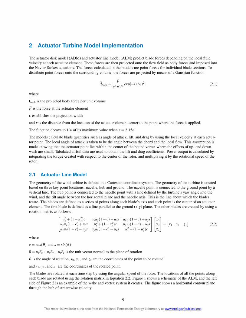

where
N is the number of blades
AB is the area of an individual section
and Ar is the swept area of the blades
The lift and drag forces on each actuator disk element are given by
L = σ 1
CL(α)ρV 2cw (26)2
D = σ 1
CD(α)ρV 2cw (27)2
Figure 4 A schematic of an actuator disk turbine model
23 Numerical Method
To use the ADM and ALM a CFD solver is used We implemented the solver using the OpenFOAM (Open Field Operation and Manipulation) toolbox [21] The OpenFOAM package is a set of C++ libraries meant for solving partial differential equations The turbine models were implemented as C++ classes called by the solver A finite-volume approach is used to discretize the governing equations The filtered Navier-Stokes equations are solved along with the standard Smagorinsky [22] model
The large eddy simulation (LES) code solves the incompressible Navier-Stokes equations The flow around wind turbines is incompressible with velocities ranging from 5-25 meters per second (ms) The incompressible filtered Navier-Stokes equations
nabla middot u = 0 (28)
part u minus+(u middot nabla)u = minus
1 nablap+ νnabla
2uminus nabla middot τSGS + rarrf turb (29)
part t ρ
are suitable for wind turbine modeling
where
u is the filtered velocity vector
p is the filtered pressure
12
This report is available at no cost from the National Renewable Energy Laboratory at wwwnrelgovpublications
ν is the kinematic viscosity
efturb is the turbine force
nabla middot τSGS = minusνSGS(nablau+(nablau)T )
and νSGS is the subgrid-scale viscosity and is modeled using the Smagorinsky subgrid-scale model
13
This report is available at no cost from the National Renewable Energy Laboratory at wwwnrelgovpublications
3 Actuator Disk and Actuator Line Models in Uniform Nonturbulent Inflow
The accuracy of the actuator disk model (ADM) and actuator line model (ALM) in predicting aerodynamic forces torque and power production depends largely on grid resolution and the projecting function To study these paramshyeters we performed a grid resolution study The solution was compared to the results that were from the NREL-developed WT_Perf [23] code which uses blade-element momentum (BEM) theory Cases were studied with differshyent values of the parameter ε which establishes the width of the Gaussian projecting function
eefturb =
F exp[minus(rε)2] (31)
ε3π32
All the meshes were created by starting with a background grid of 168-meter (m) resolution Regions of successive refinement were introduced into the background grid to provide higher resolution around the turbine and wake Each refinement region was created by splitting cells in half in each direction within that region Three different grids were made each with a different resolution that was local to the turbine and wake Those turbinewake-local resolutions were Δx = Δy = Δz =42 m 21 m and 105 m The domain was 10 rotor diameters (D) wide in all directions with the turbine rotor placed in the geometric center of the domain The finest region extended 1 diameter upstream of the turbine and 5 diameters downstream It extended 1 diameter beyond the edge of the rotor in the other two directions Figure 5 shows the mesh for a case that has three successive local refinements for a resolution of 42 m Cases were run for four different values of the ε parameter ranging from 42 m to 105 m The ALM case with ε = 84 m was tried with and without the Glauert tip loss correction [24] Cases for the ALM that had different number of actuator elements per blade span and cases with different time-step were run with a grid resolution of 21 m and ε = 84 m
Figure 5 Domain and mesh that has a turbinewake-local resolushytion of 42 m The turbine is placed in the center of the domain
31 Five Megawatt Reference Turbine
The turbine modeled was the 5-megawatt (MW) reference turbine designed by Jonkman et al [25] This horizontal-axis upwind turbine has three blades with a rotor diameter of 126 m a hub height of 90 m a rated wind speed of 114 meters per second (ms) and 5-MW-rated power production Simulations were performed with an inflow
14
This report is available at no cost from the National Renewable Energy Laboratory at wwwnrelgovpublications
condition of 8 ms The rotational speed of the rotor was fixed at 91552 revolutions per minute giving a tip speed ratio of 755 which happens to be this turbinersquos normal Region 2 tip speed ratio We chose these conditions because they provide the optimum power coefficient of the turbine and thereby extract maximum energy from the flow This is when the wakes are strongest and the wake effects are the most important
32 Actuator Line Model
Power output predicted by the ALM is shown in Figure 6 as a function of grid resolution The power output inshycreases as the grid is refined As ε becomes larger the predicted power increases The larger the ε value the smaller the rate of change of predicted power as a function of grid resolution When ε = 42 m the difference in power predicted on the finest grid and the coarsest grid is 300 kilowatts (kW) When ε = 105 m the difference is 40 kW which is much smaller Power production is clearly more grid-dependent for smaller values of ε Simulations for ε = 21 m were run with grid resolution of Δx = 105 m and 0525 m This value of ε is limited to a minimum grid resolution of 105 m because numerical instabilities appear when ε lt 2Δx The trend is followed by showing that a smaller ε will produce less power The BEM solution for power output is 1926 MW This value falls between the finest cases with ε = 42 and 21 m
Figure 7 shows time-averaged angle of attack as a function of blade length The difference in angle of attack proshyvides different lift and drag coefficients thus predicting a different force on the blades and causing different power outputs The axial velocity at the actuator element center points is shown as a function of blade length in Figure 8 It appears that a larger ε causes less axial induction at the actuator element center points (where velocity is sampled and angle of attack is computed) and also causes more power production because the force is too smoothed out
Velocity profiles through the wake along a horizontal line 1 diameter downstream at the hub height are shown in Figure 9 For the cases of ε le 63 m and Δx = 42 m the profiles have a different shape compared to all other cases When εΔx ge 32 the resolution Δx becomes important and we can observe instabilities in the results The instabilities are greater near the outmost portion of the blades where the forces are greater We observe small differences for each resolution and as the ε parameter becomes larger these differences become even smaller A grid resolution of Δx = 21 m appearss to provide converged wake profiles for each value of ε Figure 10 shows wake profiles 4 diameters downstream The profiles for the case of ε = 42 m and Δx = 42 m are affected by the numerical instabilities near the rotor which are smoothed further downstream
Mean wind speed and vorticity magnitude contours are shown in Figure 11 through Figure 16 The simulations in Figure 11 and 12 when ε = 42 m are subject to numerical instabilities These instabilities are due to the fact that εΔx = 1 where there is the limitation that ε ge 2Δx for an oscillation-free solution The velocity in the center of the wake is greater than at larger radii This is expected because the hub and nacelle are not included in the model the difference in velocity is the effect of the blades only The blades are also not as loaded at the root as they are farther outboard so they do not decelerate the flow there as much Mean speed profiles are similar for different values of ε The main difference observed is in the middle of the wake where there is a jet A larger value of ε projects the forces further beyond the root leaving a small gap between the blades for the jet to form This leaves less space for the jet as the ε value is increased As the ε value is decreased the shear layer becomes thinner and more unstable at the rotor tip and root causing a faster transition to turbulence This effect is illustrated in Figure 14 which shows that a smaller value of ε produces more vorticity The structure of the instantaneous ALM wake is not symmetric with respect to the center of the wake because the vortical structures produced by individual blades are helical and asymmetric across the wake This asymmetry causes asymmetric roll-up of Kelvin-Helmholtz-like instabilities in the outer shear layer of the wake As the grid is refined vorticity contours show more structures that are filtered in coarser grids
33 Actuator Disk Model
Power output predicted by the ADM is shown as a function of grid resolution in Figure 6 Power output increases as the grid is refined for all cases similar to the ALM Wind speed profiles through a horizontal line that are 1 diameter
15
This report is available at no cost from the National Renewable Energy Laboratory at wwwnrelgovpublications
downstream at hub height are shown in Figure 9 For the case with Δx = 42 m and ε = 42 m the solution has numerical oscillations similar to the ALM The case with Δx = 42 m and ε = 63 m has a different shape near the edge of the wake compared to the more refined cases As in the ALM this is caused by the numerical instabilities near the tip of the blade Wake profiles shown in Figure 10 appear to converge for all resolutions except when Δx = 42 m and ε = 42 m This is due to the numerical instabilities near the rotor as in the ALM cases
Mean wind speed and vorticity contours for cases with Δx = 21 m are shown in Figures 13 and 14 Mean wind speed contours are similar to the ones for the ALM Vorticity contours show the turbulent structures near the edge of the wake that are caused by the shear layer As the value of ε becomes smaller the shear layer is stronger thus increasing the turbulence in the wake (similar to what happens in the ALM) There is no formation of tip- and rootshyvortices when using the ADM These structures are formed because the bound circulation of each blade is shed at the tips in the form of vortices A continuous disk covering the swept area of the blades does not have discrete tips on which vortices are shed The wake is symmetric with respect to the center of the wake This is due to the fact that the rotor is modeled as a continuous disk rather than as individual blades There are no asymmetric helical tip-vortices to cause asymmetric Kelvin-Helmholtz-like transition to turbulence
ALM ADM
Figure 6 Power output as a function of grid resolution for different ε values
34 Actuator Points
Power output is shown as a function of blade segment resolution with ε = 84 m in Figure 17 The actuator points are distributed uniformly along the blade The resolution of the blade is presented in terms of the grid resolution (ΔbΔx) where Δb is the width of the discrete blade section and Δx is the grid resolution The number of blade sections should be high enough to predict a smooth body force field along the blades This criterion should be the basis for establishing the blade resolution A value of ΔbΔx = 3 did not predict a smooth transition through the blade thus the solution is not reliable Values below ΔbΔx = 1 predict smoothed forces along the blade The power output appears to converge after reaching a value of ΔbΔx = 05
35 Tip Loss Correction
Figure 18 shows power output as a function of grid resolution for ε = 84 m with and without a Glauert tip- and root-loss correction [24] The use of a tip- and root-loss correction makes the lift go to zero more gradually at the
16
This report is available at no cost from the National Renewable Energy Laboratory at wwwnrelgovpublications
ε = 42 m ε = 63 m
ε = 84 m ε = 105 m
Figure 7 Angle of attack as a function of blade length for the ALM
tip and root of the blade This correction decreases the total force on the blade creating less torque which results in lower power production Figure 18 illustrates this effect showing a difference of about 90 kW between the simulashytions Since the ALM produces tip-vortices that cause losses a tip-loss correction is not necessary if the tip vortices are well resolved
36 Time-step
It is advised by researchers in the field to use a Δt which allows the tip of the blade to not advance through more than one grid cell at each time-step This condition is very restrictive because it requires a time-step smaller than what would be required by the more conventional Courant-Friedrichs-Lewy (CFL) condition Figure 19 shows power output as a function of time-step for ε = 84 m This shows a linear profile with a power variation ranging from 1 to 2 This difference is small and does not suggest that the time-step is making a big difference in the simulation Figure 20 shows mean velocity and vorticity contours for different time-steps The profiles are very similar for all cases suggesting that the time-step does not cause a significant difference The value of ε = 84 used in this simulation is large A smaller ε might produce different results because the tip vortices are more pronounced As far as ε = 84 m the time-step needs to not be limited by the tip speed
17
This report is available at no cost from the National Renewable Energy Laboratory at wwwnrelgovpublications
ε = 42 m ε = 63 m
ε = 84 m ε = 105 m
Figure 8 Axial velocity as a function of blade length for the ALM
37 Comparison
The ALM and ADM predict similar wake profiles and power output The main differences between the models are 1) the vortical structures near the rotor were captured by the ALM but not by the ADM and 2) a non-symmetric wake was observed with respect to the center-line with the ALM as opposed to the symmetric wake that was obshyserved in the ADM The ALM is able to capture vortical structures that are caused by the presence of individual blades Tip and root vortices are captured when using the ALM with a high enough grid resolution as seen in Figure 14 when ε = 42 m However the ADM does not allow these structures to form only the shear layer of the wake forms
Table 1 compares power output for the ADM ALM and BEM theory A Richardson extrapolation is used to elimishynate the leading error and predict the grid-converged power solution for the ADM and ALM The power has a similar behavior for the ADM and ALM As ε becomes smaller the power output for the ADM and ALM approaches what the BEM theory predicts Both models provide similar results but as ε becomes smaller the differences are bigger
In terms of computational costs the ALM needs to rotate the blades every time-step and thus apply forces at difshyferent finite-volume cells every time-step A search for these cells is performed every time-step The ADM points are fixed and do not rotate every time-step All the cells that lie adjacent to the disk are assigned at the beginning of the simulation thus all the finite-volume cells that have an applied force are searched for only once The ADM by
18
This report is available at no cost from the National Renewable Energy Laboratory at wwwnrelgovpublications
ALM ADM
ε = 42 m
ε = 63 m
ε = 84 m
ε = 105 m
Figure 9 Mean velocity in the cross-stream direction that is 1 diameter behind the turbine rotor are shown as predicted by the ALM (left column) and ADM (right column) Each row
shows plots that are the result of using different values of the body force projection width (ε)
19
This report is available at no cost from the National Renewable Energy Laboratory at wwwnrelgovpublications
ALM ADM
ε = 42 m
ε = 63 m
ε = 84 m
ε = 105 m
Figure 10 Mean velocity in the cross-stream direction that is 4 diameters behind the turbine rotor are shown as predicted by the ALM (left column) and ADM (right column) Each row
shows plots that are the result of using different values of the body force projection width (ε)
20
This report is available at no cost from the National Renewable Energy Laboratory at wwwnrelgovpublications
ALM ADM
ε = 42 m
ε = 63 m
ε = 84 m
ε = 105 m
Figure 11 Mean velocity (ms) contours in a plane through the turbine hub are shown as predicted by the ALM (left column) and ADM (right column) with a mesh resolution of Δx = 42 m Each row shows contours that are the result of using different values of the body force projection width (ε)
Table 1 Percentage difference between the ADM ALM and BEM theory in terms of power producshytion A Richardson extrapolation is used to approximate the converged solution for the ALM and ADM
Case Predicted Power (MW) Percentage Difference with BEM ALM ADM ALM ADM
ε = 21 m 181 -60 ε = 42 m 213 214 106 110 ε = 63 m 219 219 137 137 ε = 84 m 223 223 157 157
ε = 105 m 227 227 179 179
21
This report is available at no cost from the National Renewable Energy Laboratory at wwwnrelgovpublications
ALM ADM
ε = 42 m
ε = 63 m
ε = 84 m
ε = 105 m
Figure 12 Vorticity magnitude (1s) contours in a plane through the turbine hub are shown as preshydicted by the ALM (left column) and ADM (right column) with a mesh resolution of Δx = 42 m Each
row shows contours that are the result of using different values of the body force projection width (ε)
22
This report is available at no cost from the National Renewable Energy Laboratory at wwwnrelgovpublications
ALM ADM
ε = 42 m
ε = 63 m
ε = 84 m
ε = 105 m
Figure 13 Mean velocity (ms) contours in a plane through the turbine hub are shown as predicted by the ALM (left column) and ADM (right column) with a mesh resolution of Δx = 21 m Each row shows contours that are the result of using different values of the body force projection width (ε)
23
This report is available at no cost from the National Renewable Energy Laboratory at wwwnrelgovpublications
ALM ADM
ε = 42 m
ε = 63 m
ε = 84 m
ε = 105 m
Figure 14 Vorticity magnitude (1s) contours in a plane through the turbine hub are shown as preshydicted by the ALM (left column) and ADM (right column) with a mesh resolution of Δx = 21 m Each
row shows contours that are the result of using different values of the body force projection width (ε)
24
This report is available at no cost from the National Renewable Energy Laboratory at wwwnrelgovpublications
ALM ADM
ε = 42 m
ε = 63 m
ε = 84 m
ε = 105 m
Figure 15 Mean velocity (ms) contours in a plane through the turbine hub are shown as predicted by the ALM (left column) and ADM (right column) with a mesh resolution of Δx = 105 m Each row shows contours that are the result of using different values of the body force projection width (ε)
25
This report is available at no cost from the National Renewable Energy Laboratory at wwwnrelgovpublications
ALM ADM
ε = 42 m
ε = 63 m
ε = 84 m
ε = 105 m
Figure 16 Vorticity magnitude (1s) contours in a plane through the turbine hub are shown as preshydicted by the ALM (left column) and ADM (right column) with a mesh resolution of Δx = 105 m Each row shows contours that are the result of using different values of the body force projection width (ε)
26
This report is available at no cost from the National Renewable Energy Laboratory at wwwnrelgovpublications
Figure 17 Power output for the ALM as a function of actuator point resshyolution along the blade with ε = 84 and a grid resolution of 21 m
Figure 18 Power output as a function of grid resolution for ε = 84 m with and without a tip- and root-loss correction for the ALM
contrast has more points than the ALM and the forces on these points must be calculated for every time-step These differences do not impact the simulation time significantly However time-step size will have a significant impact on simulation time The time-step for simulations performed using the ALM is restricted by the tip speed The tip
27
This report is available at no cost from the National Renewable Energy Laboratory at wwwnrelgovpublications
Figure 19 Power output as a function of time-step for ε = 84 m
of the blade should not pass through more than a single finite-volume cell each time-step This condition is far more restrictive than the typical CFL condition For a case with λ =8 the time-step needs to be eight times smaller using this restriction than with the CFL condition Resolving the root- and tip-vortices compromises the simulation time-step and thus increases computational cost The ADM will provide an accurate solution with a time-step that is based on a CFL condition rather than on tip speed If the simulations require solving the flow structures near the rotor the ALM should be used For simulations related to the far wake the ADM will provide a reasonable solution without compromising the simulation time-step
38 The ε Parameter
A Gaussian function is introduced to turn the set of unphysical point forces into a continuous volume force field The use of a Gaussian function avoids numerical instabilities caused by the application of forces on discrete sections of the blade The width of the function is determined by the ε parameter This parameter plays an important role in the models studied We found that a parameter closest to the characteristic length of the blade section under study yielded the best results The value of the Gaussian function decays to 1 of its initial value at a distance of r = 215ε To span the force of a blade section through the area that covers the distance from the leading edge to the trailing edge a value of ε = c43 would be required With a chord value around 4 m for the NREL 5-MW turbine a value of ε = 4 m43 = 093 m creates numerical instabilities on the grids used in this study Our projections show that making the grid smaller would be expensive unless a fine grid local to the rotor was used
The simulations presented show that as ε becomes smaller the power decreases Note that a small value of ε relashytive to the grid size produces numerical instabilities in the solver These instabilities affect the solution and can be observed in the wake profiles and angle of attack for a case in which ε = 42 m and a grid resolution of 42 m When parameter ε was the same size as the grid size (εΔx = 1) the simulations for the ALM and ADM became unstable This can be avoided by choosing a value of εΔx gt 2 as suggested by Troldborg [9] There is an optimum point for the Gaussian width to match what the BEM theory predicts This optimum is related to the geometry of the blade In this case the solution given by the BEM theory lies somewhere between ε =42 and 21 m It is unclear which value of ε matches the geometry of the blade section and would accurately predict power using the ALM The results
28
This report is available at no cost from the National Renewable Energy Laboratory at wwwnrelgovpublications
Vorticity Mean Velocity
Δt = 0015s
Δt = 003s
Δt = 006s
Δt = 01s
Figure 20 Mean velocity (ms) and vorticity magnitude (1s) contours in a plane through the turbine hub for ε = 84 m are shown Each row shows contours that are the result of using different time-step values
29
This report is available at no cost from the National Renewable Energy Laboratory at wwwnrelgovpublications
suggest that the value of ε should not be fixed to a value that satisfies the condition that ε = c43 A condition that better approximates the physical force distribution of an airfoil should be used varying ε along the span as the chord varies
Increasing the value of ε thickens the shear layer surrounding the wake As the shear layer is thickened there is less vorticity in the flow This is illustrated in Figures 12 14 and 16 as the vorticity decreases with larger ε
30
This report is available at no cost from the National Renewable Energy Laboratory at wwwnrelgovpublications
4 Wind Tunnel Simulations
We have performed a validation of the actuator line model (ALM) that compares the numerical results with the experiments done at the low-speed closed-return wind tunnel at the Department of Energy and Process Engineering at the Norwegian University of Science and Technology Trondheim [26][27] The tunnel has a test section of 185 meters (m) (height) times 271 m (width) times 1115 m (length) The test section height is adjustable to account for wall boundary layer growth In this study we aimed to numerically simulate the experimental setup
We performed simulations for tip speed ratios (λ ) of 3 4 6 9 and 12 and compared the power and thrust coefshyficients against the experimental data In addition we used wake visualizations to illustrate the difference in the breakdown of the wake for different tip speed ratios as well as sampled wake profiles
41 Turbine Model
The turbine modeled has a rotor with a diameter of 0894 m and a tower with a height of 0817 m The blades use the National Renewable Energy Laboratory (NREL) S826 airfoil along the entire span We obtained two-dimensional lift and drag coefficients from the NREL S826 report [28] and corrected for stall delay using NRELrsquos AirfoilPrep tool [29] The actuator line model accounts for only the blades of the turbine and does not include the hub tower or nacelle The turbine is located 366 m from the tunnel inlet and is laterally centered
42 Mesh
The mesh of the tunnel consists of a block with dimensions (1115 m times 1851 m times 271 m) The walls are refined in an attempt to capture the boundary layer The height of the tunnel varies linearly along the streamwise direction from 1801 m to 1851 m The mesh is refined near the walls to capture the boundary layer The walls have a no-slip condition The grid resolution near the wall does not resolve the boundary layer completely but because the rotor is far from the walls we believe the effect of not resolving this boundary layer is negligible The mesh is locally refined near the rotor with ΔxD = 0006 This refinement allows the simulation to calculate power production accurately (following the results from the previous section)
The boundary layer is measured to be 01 m at the tunnel inlet The inlet bulk velocity is taken to be 10 meters per second (ms) The inlet boundary condition is set to match the turbulent boundary layer profile using y 17
U = (41)δ
At y gt δ the velocity is set to 10 ms with no turbulence
43 Results
Power and thrust coefficients are shown as a function of tip speed ratio in Figure 21 The maximum power coeffishycient of 047 is at a tip speed ratio of 6 This corresponds to the highest induction factor as we expected For the case with lowest tip speed ratio the simulation power coefficient lies on top of the experimental data Thrust coefficient is under-predicted for all tip speed ratios
Figure 22 shows wake profiles in the spanwise direction for 1 2 3 and 4 diameters behind the rotor The profiles show how the wake deficit is stronger for higher tip speed ratios Note that for stronger wake deficits the velocity near the edges and in the center of the rotor is larger because of mass conservation Figure 23 shows wake profiles for cases with tip speed ratios of 3 and 6 that are one diameter behind the rotor The wakes in the simulation are different from the experimental data at the center This difference is because the nacelle is not a part of the model It is clear that the nacelle needs to be incorporated into the model to obtain accurate wake profiles As a result this
31
This report is available at no cost from the National Renewable Energy Laboratory at wwwnrelgovpublications
difference causes the thrust to be lower than expected because the nacelle will contribute a drag force to the model For this reason the thrust coefficient curve for the simulations lies below the experimental data Away from the center the wake profiles agree with the experimental data
Figure 24 shows a rendering of the Q-criterion [30] for tip speed ratios of λ = 3 6 9 and 12 The Q-criterion is the second invariant of the velocity gradient tensor Where it is positive it shows regions of the flow where rotation dominates strain and where it is negative strain dominates rotation This illustrates that the breakdown of the wake is faster with increased tip speed ratio With higher tip speed ratio the wake deficit is greater as shown in Figure 22 indicating there is a stronger more unstable wake-edge shear layer This causes faster transition to turbulence and faster wake breakdown The visualizations show that at higher tip speeds the wake starts interacting with the tunnel walls This interaction affects the wake as it is not able to fully expand
The ALM is a good representation of the turbine in the tunnel but is missing some key elements in its implementashytion The model is able to capture the blades inside the flow field Because the power of the turbine is being extracted by the blades the power coefficient is close to what experiments predict However the effect of the nacelle is not included in the model The nacelle contributes to the thrust experienced by the turbine and for this reason the thrust coefficient is under-predicted by the model Tip speed ratio affects the power produced by the turbine and the strucshyture of the wake The maximum power coefficient is reached at a tip speed ratio of 6 which approximates the Betz limit A faster tip speed ratio causes a faster breakdown of the wake
Power Thrust
Figure 21 Power and thrust coefficients as a function of tip speed ratio
32
This report is available at no cost from the National Renewable Energy Laboratory at wwwnrelgovpublications
xD = 1 xD = 2
xD = 3 xD = 4
Figure 22 Mean velocity profiles behind the rotor
33
This report is available at no cost from the National Renewable Energy Laboratory at wwwnrelgovpublications
1D TSR=3 1D TSR=6
3D TSR=3 3D TSR=6
Figure 23 Mean velocity profiles one and three diameters behind the rotor
34
This report is available at no cost from the National Renewable Energy Laboratory at wwwnrelgovpublications
λ = 3 λ = 6
λ = 9 λ = 12
Figure 24 Q-criterion (1s2) rendering showing the structure of the wake for different tip speed ratios
35
This report is available at no cost from the National Renewable Energy Laboratory at wwwnrelgovpublications
5 Wind Farm Simulation
51 Introduction
This section presents the results of a large-eddy simulation (LES) of the flow of over 48 multi-megawatt turbines that compose the Lillgrund wind plant We compared the performance of the actuator line (ALM) and actuator disk model (ADM) in wind farm simulations Churchfield et al [31] performed an LES of the Lillgrund wind farm using the ALM we performed the same simulation using the ADM and compared the results for both models The simulated wind farm is the Lillgrund offshore facility operated by Vattenfall Vindkraft AB Lillgrund is located 7 kilometers (km) off the coast of Sweden and 7 km south of the Oumlresund bridge Figure 25 shows the turbine siting and the computational domain Positive x and y correspond to east and north respectively
We used LES to simulate the atmospheric boundary layer (ABL) with the standard Smagorinsky model We modeled the sea surface as a rough flat surface with an aerodynamic roughness height of 01 millimiters (mm) which was appropriate for the sea surface The turbine model operating at the Lillgrund facility is the Siemens SWT-23-93 The turbine model was provided by Churchfield who reverse-engineered the available turbine information [32] We performed the simulation in two steps running an ABL precursor simulation and running the wind plant simulation The first precursor simulation tried to match the Lillgrund wind conditions as closely as possible and was obtained from Churchfield [31] We chose a mean velocity of 9 ms at hub-height with a wind direction of 2216o At these conditions the turbines operating in Region 2 wake deficits are the strongest We used the turbulent intensity at hub-height of 62 which is typical at the chosen wind direction The precursor simulation was used to create a turbulent wind inlet (west and south) boundary condition on velocity and temperature for the simulation The east and north planes were set to zero gradient for velocity and temperature The velocity top boundary condition was set to zero in the normal direction and to zero gradient in the other two directions The pressure boundary conditions were set to hydrostatic gradient on the top and bottom and to zero gradient on the sides The temperature gradient on the top was set to 0003 Kelvins per meter (Km) to follow the temperature profile in capping inversion The precursor simulation was the same for both the ADM and ALM simulation The time-step of the ALM simulation was fixed at the condition that the tip of the blade should not go through more than one grid cell at each time-step The time-step in the ADM simulation was based on the maximum Courant number not exceeding a limit of 075 The wind plant simulation was for 10 minutes of real time and an initial transient of 150 s
52 Results
Normalized power output is shown for all the rows in the turbine array in Figure 26 Rows B through D are comshypared against field data that were averaged over a year and binned by wind direction Power output for these rows is normalized using the average power of the first turbine in rows B C and D The other turbines are normalized using the power of the first turbine in their row The simulations agree with field data The largest difference is on the last turbines in the rows where the simulation predicted an increase in power production Figure 27 shows non-normalized power output for all the turbines Power production for the ADM agrees well with that for ALM although we observe slight differences The percent difference between the ADM and ALM dimensional power flucshytuated between 1 and 17 Contrasting what we observed in Chapter 3 the ALM produces a slightly higher power output than the ADM The power curve for the model predicts 1347 megawatts (MW) at 9 ms The first turbine in each row is close to this value for both the ADM and ALM although we observed that the ALM usually over predicts power whereas the ADM under predicts power
Figure 28 shows the mean velocity profiles for the ADM and ALM The wake deficits in the ADM simulation are stronger (shown in dark blue) than the ALM Figure 29 shows the difference between the ADM and ALM simulashytions which was calculated by subtracting the ADM data from the ALM data The figure reveals that the regions near the center of the wake have the strongest difference (shown in red)
Figure 30 shows wake profiles along rows C and E The profiles pass through the hub and outboard of the hub in increments of D8 where D is the rotor diameter This shows the wake differences between the models at several
36
This report is available at no cost from the National Renewable Energy Laboratory at wwwnrelgovpublications
Figure 25 Wind farm layout (left) and computational doshymain (right) Illustration by Matthew J Churchfield NREL
locations The biggest difference in wake profiles is on the wake of the first turbine in each row The ADM creates a larger velocity deficit in the center when passing through the first turbine The flow begins to recover in the far wake before hitting the next turbines The ALM and ADM recover to nearly the same value This pattern repeats until the last turbine in the row There is a gap in row E where the flow recovers more than the rest of the turbines This recovery produces more power on the next turbine in the row although the flow is not fully recovered A power production difference of 30 was observed between the turbine right after the gap and the subsequent one The wake recovery in the gap allows greater power production from the next turbine in the row Field data always show a slight increase in power of the third turbine over the second turbine in the row The ALM does not predict this but the ADM does
Figures 32 33 and 34 show wake profiles for turbines 27 through 30 and at 05 075 and 1 diameter behind the rotor The profiles show that the velocity deficit near the center of the wake for the ADM is stronger than that of the ALM However moving towards the edge of the wake the velocity deficit from the ALM is stronger than for the ADM
The time-step used for the ALM simulation was Δt =0015 s while the time-step for the ADM simulation was based on a Courant-Friedrichs-Lewy number of 075 with typical values close to Δt =006 s The difference in time-step may cause the power output differences that were observed Figure 19 shows that as Δt increases predicted power decreases similar to what Figure 27 shows
The ADM simulation was completed two times faster than the ALM simulation The ALM simulation required about 1 million CPU-hours whereas the ADM showed significant savings This difference is because the ADM has a higher time-step On a time per time-step basis the ADM takes longer to calculate all the body forces on the disk (rather than just the body forces on the blades of the ALM)
The ALM and ADM provide similar results in large-scale wind farm simulations There is a difference in power production in which the ALM produces more power than the ADM The difference in the first row of turbines is larger than the turbines that are further downstream In terms of computational cost the ADM can be run faster because time-step is not limited to tip speed The ADM simulation was completed three times faster than the ALM This time reduction is crucial when performing these type of simulations The wake in the ADM has a greater deficit
37
This report is available at no cost from the National Renewable Energy Laboratory at wwwnrelgovpublications
in the center than the ALM However the velocity deficit near the edges is stronger for the ALM indicating a larger power extraction is near the outer portion of the blades The total difference shows that the power extraction for the ALM is greater than that for the ADM
38
This report is available at no cost from the National Renewable Energy Laboratory at wwwnrelgovpublications
Row A Row B
Row C Row D
Row E Row F
Row G Row H
macrFigure 26 Ten minute average power produced by each turbine Pi normalized by the power of the first turbine in the row Average over one year of field data is shown for rows B-D
39
This report is available at no cost from the National Renewable Energy Laboratory at wwwnrelgovpublications
Row A Row B
Row C Row D
Row E Row F
Row G Row H
Figure 27 Power produced by each turbine
40
This report is available at no cost from the National Renewable Energy Laboratory at wwwnrelgovpublications
ADM ALM
Figure 28 Mean velocity (ms) contours at hub height for ADM (left) and ALM (right)
Figure 29 Mean velocity difference (ms) between ALM and ADM (ALM-ADM)
41
This report is available at no cost from the National Renewable Energy Laboratory at wwwnrelgovpublications
Row C Row E
yR = 0
yR = 025
yR = 05
yR = 075
yR = 1
Figure 30 Mean streamwise velocity profiles at hub height along rows C and E at various horizontal locations outboard of hub ranging from hub to blade tip
Turbine 30 Turbine 29
Turbine 28 Turbine 27
Figure 31 Mean velocity in the cross stream direction at one-fourth diameter behind the rotor for turbines in row D
42
This report is available at no cost from the National Renewable Energy Laboratory at wwwnrelgovpublications
Turbine 30 Turbine 29
Turbine 28 Turbine 27
Figure 32 Mean velocity in the cross stream direction at one-half diameter behind the rotor for turbines in row D
Turbine 30 Turbine 29
Turbine 28 Turbine 27
Figure 33 Mean velocity in the cross stream direction at three-fourths diameter behind the rotor for turbines in row D
43
This report is available at no cost from the National Renewable Energy Laboratory at wwwnrelgovpublications
Turbine 30 Turbine 29
Turbine 28 Turbine 27
Figure 34 Mean velocity in the cross stream direction at 1 diameter behind the rotor for turbines in row D
Turbine 30 Turbine 29
Turbine 28 Turbine 27
Figure 35 Mean velocity in the cross stream direction at 3 diameters behind the rotor for turbines in row D
44
This report is available at no cost from the National Renewable Energy Laboratory at wwwnrelgovpublications
Turbine 30 Turbine 29
Turbine 28 Turbine 27
Figure 36 Mean velocity in the cross stream direction at 4 diameters behind the rotor for turbines in row D
45
This report is available at no cost from the National Renewable Energy Laboratory at wwwnrelgovpublications
6 Conclusion and Future Work
The actuator line model (ALM) and actuator disk model (ADM) are a suitable representation of a wind turbine when using numerical simulations of fluid flows The models do not require that the full geometry of the blades be resolved and in which case model them as a set of points in the flow The ALM models the blades as a set of points along each blade axis whereas the ADM models the rotor as a disk with points that represent sections of the disk
The ADM and ALM provide very similar results in simulations with uniform inflow There is a clear grid depenshydence on power production and wake profiles of the ADM and ALM As the grid is refined the predicted power increases for both models Using a Glauert tip-loss correction with the ALM decreases the power production The number of actuator points in the ALM should be adequate to account for all the sections of the blade and provide smooth changes between them We recommend using a value smaller than ΔbΔx = 075 Mean wake profiles are similar for both the ADM and ALM
A Gaussian function was introduced to avoid numerical instabilities that are caused by the application of forces on discrete sections of the blade The width of the function was determined by the ε parameter This parameter played an important role in the models studied We observed that a parameter closest to the characteristic length of the blade section yielded the best results As the width of the projection function is decreased both the ALM and ADM predicted power decreases but never converges upon a value A specific value of epsilon allows agreement with blade-element momentum theory predictions However the ε parameter must be higher than 2Δx to avoid numerical instabilities in the solver
The ALM resolves the flow structures that are caused by the presence of individual blades which the ADM does not The ALM matches the physics more closely because it captures the root- and tip-vortices which the ADM does not Also the ALM is able to capture helical and asymmetric structures across the wake which caused asymmetric roll-up of Kelvin-Helmholtz-like instabilities in the wakersquos outer shear layer The ALM captures the vortical structures in the near wake ADM provides good results in the far wake but does not produce the vortical structures near the rotor If simulations are intended to determine the far wake effects the ADM should provide reasonable results
We used the ALM to validate a small-scale wind tunnel experiment and compared the structure of the wake for different tip speed ratios We observed that as the tip speed ratio is higher the breakdown of the wake occurs faster leaving a wider wake for larger tip speed ratios The tunnel walls play an important role in the simulation as the wake interacts with the walls The blockage effect of the turbine makes the reference velocity of the tunnel higher near the rotor than on the inlet
When performing large-scale wind farm simulations we found that the models perform well ALM produces slightly more power than ADM under atmospheric boundary layer conditions It is still unknown why this occurs but it is possible that the difference is caused by the time-step difference in the simulations The wake of the ADM is different from that of the ALM The ADM wake has a stronger wake deficit near the center whereas the ALM has a stronger wake deficit near the edges Wake profiles are similar but we observed that the greatest difference in the near wake primarily in the first row of turbines
46
This report is available at no cost from the National Renewable Energy Laboratory at wwwnrelgovpublications
Bibliography
[1] JN Soslashrensen Aerodynamics aspects of wind energy conversion 43427ndash448 September 2010
[2] T Burton D Sharpe N Jenkins and E Bossanyi Aerodynamics of Horizontal-Axis Wind Turbines pages 41ndash172 John Wiley amp Sons Ltd 2002
[3] JF Manwell JG McGowan and AL Rogers Wind Energy Explained Theory Design and Application Wiley 2010
[4] B Sanderse SP van der Pijl and B Koren Review of computational fluid dynamics for wind turbine wake aerodynamics Wind Energy 14 2011
[5] F Porteacute-Agel H Lu and YT Wu A Large-Eddy simulation framework for wind energy applications The Fifth International Symposium on Computational Wind Engineering (CWE2010) Chapel Hill North Carolina USA May 23-27 2010
[6] M Calaf C Meneveau and J Meyers Large eddy simulation study of fully developed wind-turbine array boundary layers Physics of Fluids 22(1)015110 2010
[7] N Troldborg JN Soslashrensen and R Mikkelsen Numerical simulations of wake charasteristics of a wind turbine in uniform flow 1386ndash99 2009
[8] T Phuoc Aeacuterodynamique instationnaire turbulente - aspects numeacuteriques et expeacuterimentaux Journeacute theacutematique DRET 1994
[9] N Troldborg Actuator Line Modeling of Wind Turbine Wakes PhD thesis Technical University of Denmark Lyngby Denmark 2008
[10] I Ammara C Leclerc and C Masson A viscous three-dimensional differentialactuator-disk method for the aerodynamic analysis of wind farms Journal of Solar Energy Engineering 124(4)345ndash356 2002
[11] A Jimenez A Crespo E Migoya and J Garcia Advances in large-eddy simulation of a wind turbine wake Journal of Physics Conference Series 75(1)012041 2007
[12] C Masson A Smaiumlli and C Leclerc Aerodynamic analysis of hawts operating in unsteady conditions Wind Energy 4(1)1ndash22 2001
[13] R Mikkelsen JN Soslashrensen and WZ Shen Modelling and analysis of the flow field around a coned rotor Wind Energy 4(3)121ndash135 2001
[14] JN Soslashrensen and WZ Shen Numerical modeling of wind turbine wakes Journal of Fluids Engineering 124(2)393ndash399 June 2002
[15] SSA Ivanell JN Soslashrensen R Mikkelsen and D Henningson Analysis of numerically generated wake structures Wind Energy 12(1)63ndash80 2009
[16] R Mikkelsen JN Soslashrensen S Oslashye and N Troldborg Analysis of power enhancement for a row of wind turbines using the actuator line technique Journal of Physics Conference Series ndash The Science of Making Torque from Wind 75(012044) 2007
[17] R Mikkelsen Actuator Disc Methods Applied to Wind Turbines PhD thesis Technical University of Denmark Mechanical Engineering Department 2003
[18] WZ Shen JH Zhang and JN Soslashrensen The actuator surface model A new navierndashstokes based model for rotor computations Journal of Solar Energy Engineering 131(1)011002 2009
47
This report is available at no cost from the National Renewable Energy Laboratory at wwwnrelgovpublications
[19] I Dobrev F Massouh and M Rapin Actuator surface hybrid model Journal of Physics Conference Series 75(1)012019 2007
[20] CS Watters and C Masson Modeling of lifting-device aerodynamics using the actuator surface concept International Journal for Numerical Methods in Fluids 62(11)1264ndash1298 2010
[21] OpenFOAM Ver 171 [available online] Silicon Graphics International Corporation (SGI) URL httpwwwopenfoamorgarchive171download [accessed 13 December 2011]
[22] J Smagorinsky General circulation experiments with the primitive equations Monthly Weather Review 9199ndash164 1963
[23] MJ Buhl WT_Perf Userrsquos Guide National Renewable Energy Laboratory 2004
[24] H Glauert Airplane Propellers pages 251ndash268 Dover New York 1985
[25] J Jonkman S Butterfield W Musial and G Scott Definition of a 5-MW reference wind turbine for offshore system development Technical Report NRELTP-500-38060
[26] MS Adaramola and P-A Krogstad Experimental investigation of wake effects on wind turbine performance Renewable Energy 362078ndash2086 2011
[27] P-A Krogstad and JA Lund An experimental and numerical study of the performance of a model turbine Wind Energy 2011
[28] DM Somers The S825 and S826 Airfoils Period of Performance 1994ndash1995 The S825 and S826 Airfoils Technical Report January 2005
[29] NWTC Design Codes (AirfoilPrep by Dr Craig Hansen) httpwindnrelgovdesigncodespreprocessorsairfoilprep [Accessed 21 February 2012]
[30] JCR Hunt AA Wray and P Moin Eddies streams and convergence zones in turbulent flows (1970) 1988
[31] MJ Churchfield S Lee P Moriarty LA Martiacutenez S Leonardi G Vijayakumar and JG Brasseur A large-eddy simulation of wind-plant aerodynamics 50th AIAA Aerospace Sciences Meeting Nashville Tennessee USA 2012
[32] MJ Churchield A Method for Designing Generic Wind Turbine Models Representative of Real Turbines and Generic Siemens SWT-23-93 and Vestas V80 Specifications National Renewable Energy Laboratory 2012
48
This report is available at no cost from the National Renewable Energy Laboratory at wwwnrelgovpublications
- Literature Review
-
- Introduction
- Basics of Wind Turbine Aerodynamics
- Wind Turbine Computational Fluid Dynamics
- Atmospheric Boundary Layer Simulations
- Actuator Disc Model (ADM)
- Actuator Line Model (ALM)
- Actuator Surface Model (ASM)
- Comparison Between ADM and ALM
- Conclusions
-
- Actuator Turbine Model Implementation
-
- Actuator Line Model
- Actuator Disk Model
- Numerical Method
-
- Actuator Disk and Actuator Line Models in Uniform Nonturbulent Inflow
-
- Five Megawatt Reference Turbine
- Actuator Line Model
- Actuator Disk Model
- Actuator Points
- Tip Loss Correction
- Time-step
- Comparison
- The Parameter
-
- Wind Tunnel Simulations
-
- Turbine Model
- Mesh
- Results
-
- Wind Farm Simulation
-
- Introduction
- Results
-
- Conclusion and Future Work
- Bibliography
-
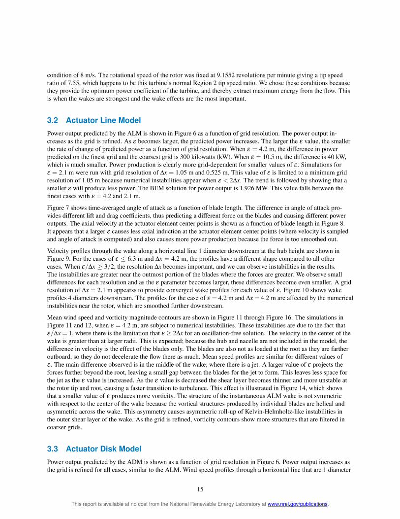
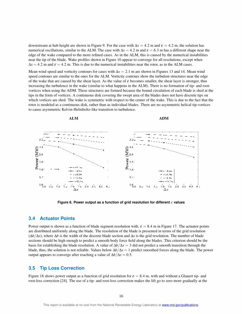
ε = 42 m ε = 63 m
ε = 84 m ε = 105 m
Figure 7 Angle of attack as a function of blade length for the ALM
tip and root of the blade This correction decreases the total force on the blade creating less torque which results in lower power production Figure 18 illustrates this effect showing a difference of about 90 kW between the simulashytions Since the ALM produces tip-vortices that cause losses a tip-loss correction is not necessary if the tip vortices are well resolved
36 Time-step
It is advised by researchers in the field to use a Δt which allows the tip of the blade to not advance through more than one grid cell at each time-step This condition is very restrictive because it requires a time-step smaller than what would be required by the more conventional Courant-Friedrichs-Lewy (CFL) condition Figure 19 shows power output as a function of time-step for ε = 84 m This shows a linear profile with a power variation ranging from 1 to 2 This difference is small and does not suggest that the time-step is making a big difference in the simulation Figure 20 shows mean velocity and vorticity contours for different time-steps The profiles are very similar for all cases suggesting that the time-step does not cause a significant difference The value of ε = 84 used in this simulation is large A smaller ε might produce different results because the tip vortices are more pronounced As far as ε = 84 m the time-step needs to not be limited by the tip speed
17
This report is available at no cost from the National Renewable Energy Laboratory at wwwnrelgovpublications
ε = 42 m ε = 63 m
ε = 84 m ε = 105 m
Figure 8 Axial velocity as a function of blade length for the ALM
37 Comparison
The ALM and ADM predict similar wake profiles and power output The main differences between the models are 1) the vortical structures near the rotor were captured by the ALM but not by the ADM and 2) a non-symmetric wake was observed with respect to the center-line with the ALM as opposed to the symmetric wake that was obshyserved in the ADM The ALM is able to capture vortical structures that are caused by the presence of individual blades Tip and root vortices are captured when using the ALM with a high enough grid resolution as seen in Figure 14 when ε = 42 m However the ADM does not allow these structures to form only the shear layer of the wake forms
Table 1 compares power output for the ADM ALM and BEM theory A Richardson extrapolation is used to elimishynate the leading error and predict the grid-converged power solution for the ADM and ALM The power has a similar behavior for the ADM and ALM As ε becomes smaller the power output for the ADM and ALM approaches what the BEM theory predicts Both models provide similar results but as ε becomes smaller the differences are bigger
In terms of computational costs the ALM needs to rotate the blades every time-step and thus apply forces at difshyferent finite-volume cells every time-step A search for these cells is performed every time-step The ADM points are fixed and do not rotate every time-step All the cells that lie adjacent to the disk are assigned at the beginning of the simulation thus all the finite-volume cells that have an applied force are searched for only once The ADM by
18
This report is available at no cost from the National Renewable Energy Laboratory at wwwnrelgovpublications
ALM ADM
ε = 42 m
ε = 63 m
ε = 84 m
ε = 105 m
Figure 9 Mean velocity in the cross-stream direction that is 1 diameter behind the turbine rotor are shown as predicted by the ALM (left column) and ADM (right column) Each row
shows plots that are the result of using different values of the body force projection width (ε)
19
This report is available at no cost from the National Renewable Energy Laboratory at wwwnrelgovpublications
ALM ADM
ε = 42 m
ε = 63 m
ε = 84 m
ε = 105 m
Figure 10 Mean velocity in the cross-stream direction that is 4 diameters behind the turbine rotor are shown as predicted by the ALM (left column) and ADM (right column) Each row
shows plots that are the result of using different values of the body force projection width (ε)
20
This report is available at no cost from the National Renewable Energy Laboratory at wwwnrelgovpublications
ALM ADM
ε = 42 m
ε = 63 m
ε = 84 m
ε = 105 m
Figure 11 Mean velocity (ms) contours in a plane through the turbine hub are shown as predicted by the ALM (left column) and ADM (right column) with a mesh resolution of Δx = 42 m Each row shows contours that are the result of using different values of the body force projection width (ε)
Table 1 Percentage difference between the ADM ALM and BEM theory in terms of power producshytion A Richardson extrapolation is used to approximate the converged solution for the ALM and ADM
Case Predicted Power (MW) Percentage Difference with BEM ALM ADM ALM ADM
ε = 21 m 181 -60 ε = 42 m 213 214 106 110 ε = 63 m 219 219 137 137 ε = 84 m 223 223 157 157
ε = 105 m 227 227 179 179
21
This report is available at no cost from the National Renewable Energy Laboratory at wwwnrelgovpublications
ALM ADM
ε = 42 m
ε = 63 m
ε = 84 m
ε = 105 m
Figure 12 Vorticity magnitude (1s) contours in a plane through the turbine hub are shown as preshydicted by the ALM (left column) and ADM (right column) with a mesh resolution of Δx = 42 m Each
row shows contours that are the result of using different values of the body force projection width (ε)
22
This report is available at no cost from the National Renewable Energy Laboratory at wwwnrelgovpublications
ALM ADM
ε = 42 m
ε = 63 m
ε = 84 m
ε = 105 m
Figure 13 Mean velocity (ms) contours in a plane through the turbine hub are shown as predicted by the ALM (left column) and ADM (right column) with a mesh resolution of Δx = 21 m Each row shows contours that are the result of using different values of the body force projection width (ε)
23
This report is available at no cost from the National Renewable Energy Laboratory at wwwnrelgovpublications
ALM ADM
ε = 42 m
ε = 63 m
ε = 84 m
ε = 105 m
Figure 14 Vorticity magnitude (1s) contours in a plane through the turbine hub are shown as preshydicted by the ALM (left column) and ADM (right column) with a mesh resolution of Δx = 21 m Each
row shows contours that are the result of using different values of the body force projection width (ε)
24
This report is available at no cost from the National Renewable Energy Laboratory at wwwnrelgovpublications
ALM ADM
ε = 42 m
ε = 63 m
ε = 84 m
ε = 105 m
Figure 15 Mean velocity (ms) contours in a plane through the turbine hub are shown as predicted by the ALM (left column) and ADM (right column) with a mesh resolution of Δx = 105 m Each row shows contours that are the result of using different values of the body force projection width (ε)
25
This report is available at no cost from the National Renewable Energy Laboratory at wwwnrelgovpublications
ALM ADM
ε = 42 m
ε = 63 m
ε = 84 m
ε = 105 m
Figure 16 Vorticity magnitude (1s) contours in a plane through the turbine hub are shown as preshydicted by the ALM (left column) and ADM (right column) with a mesh resolution of Δx = 105 m Each row shows contours that are the result of using different values of the body force projection width (ε)
26
This report is available at no cost from the National Renewable Energy Laboratory at wwwnrelgovpublications
Figure 17 Power output for the ALM as a function of actuator point resshyolution along the blade with ε = 84 and a grid resolution of 21 m
Figure 18 Power output as a function of grid resolution for ε = 84 m with and without a tip- and root-loss correction for the ALM
contrast has more points than the ALM and the forces on these points must be calculated for every time-step These differences do not impact the simulation time significantly However time-step size will have a significant impact on simulation time The time-step for simulations performed using the ALM is restricted by the tip speed The tip
27
This report is available at no cost from the National Renewable Energy Laboratory at wwwnrelgovpublications
Figure 19 Power output as a function of time-step for ε = 84 m
of the blade should not pass through more than a single finite-volume cell each time-step This condition is far more restrictive than the typical CFL condition For a case with λ =8 the time-step needs to be eight times smaller using this restriction than with the CFL condition Resolving the root- and tip-vortices compromises the simulation time-step and thus increases computational cost The ADM will provide an accurate solution with a time-step that is based on a CFL condition rather than on tip speed If the simulations require solving the flow structures near the rotor the ALM should be used For simulations related to the far wake the ADM will provide a reasonable solution without compromising the simulation time-step
38 The ε Parameter
A Gaussian function is introduced to turn the set of unphysical point forces into a continuous volume force field The use of a Gaussian function avoids numerical instabilities caused by the application of forces on discrete sections of the blade The width of the function is determined by the ε parameter This parameter plays an important role in the models studied We found that a parameter closest to the characteristic length of the blade section under study yielded the best results The value of the Gaussian function decays to 1 of its initial value at a distance of r = 215ε To span the force of a blade section through the area that covers the distance from the leading edge to the trailing edge a value of ε = c43 would be required With a chord value around 4 m for the NREL 5-MW turbine a value of ε = 4 m43 = 093 m creates numerical instabilities on the grids used in this study Our projections show that making the grid smaller would be expensive unless a fine grid local to the rotor was used
The simulations presented show that as ε becomes smaller the power decreases Note that a small value of ε relashytive to the grid size produces numerical instabilities in the solver These instabilities affect the solution and can be observed in the wake profiles and angle of attack for a case in which ε = 42 m and a grid resolution of 42 m When parameter ε was the same size as the grid size (εΔx = 1) the simulations for the ALM and ADM became unstable This can be avoided by choosing a value of εΔx gt 2 as suggested by Troldborg [9] There is an optimum point for the Gaussian width to match what the BEM theory predicts This optimum is related to the geometry of the blade In this case the solution given by the BEM theory lies somewhere between ε =42 and 21 m It is unclear which value of ε matches the geometry of the blade section and would accurately predict power using the ALM The results
28
This report is available at no cost from the National Renewable Energy Laboratory at wwwnrelgovpublications
Vorticity Mean Velocity
Δt = 0015s
Δt = 003s
Δt = 006s
Δt = 01s
Figure 20 Mean velocity (ms) and vorticity magnitude (1s) contours in a plane through the turbine hub for ε = 84 m are shown Each row shows contours that are the result of using different time-step values
29
This report is available at no cost from the National Renewable Energy Laboratory at wwwnrelgovpublications
suggest that the value of ε should not be fixed to a value that satisfies the condition that ε = c43 A condition that better approximates the physical force distribution of an airfoil should be used varying ε along the span as the chord varies
Increasing the value of ε thickens the shear layer surrounding the wake As the shear layer is thickened there is less vorticity in the flow This is illustrated in Figures 12 14 and 16 as the vorticity decreases with larger ε
30
This report is available at no cost from the National Renewable Energy Laboratory at wwwnrelgovpublications
4 Wind Tunnel Simulations
We have performed a validation of the actuator line model (ALM) that compares the numerical results with the experiments done at the low-speed closed-return wind tunnel at the Department of Energy and Process Engineering at the Norwegian University of Science and Technology Trondheim [26][27] The tunnel has a test section of 185 meters (m) (height) times 271 m (width) times 1115 m (length) The test section height is adjustable to account for wall boundary layer growth In this study we aimed to numerically simulate the experimental setup
We performed simulations for tip speed ratios (λ ) of 3 4 6 9 and 12 and compared the power and thrust coefshyficients against the experimental data In addition we used wake visualizations to illustrate the difference in the breakdown of the wake for different tip speed ratios as well as sampled wake profiles
41 Turbine Model
The turbine modeled has a rotor with a diameter of 0894 m and a tower with a height of 0817 m The blades use the National Renewable Energy Laboratory (NREL) S826 airfoil along the entire span We obtained two-dimensional lift and drag coefficients from the NREL S826 report [28] and corrected for stall delay using NRELrsquos AirfoilPrep tool [29] The actuator line model accounts for only the blades of the turbine and does not include the hub tower or nacelle The turbine is located 366 m from the tunnel inlet and is laterally centered
42 Mesh
The mesh of the tunnel consists of a block with dimensions (1115 m times 1851 m times 271 m) The walls are refined in an attempt to capture the boundary layer The height of the tunnel varies linearly along the streamwise direction from 1801 m to 1851 m The mesh is refined near the walls to capture the boundary layer The walls have a no-slip condition The grid resolution near the wall does not resolve the boundary layer completely but because the rotor is far from the walls we believe the effect of not resolving this boundary layer is negligible The mesh is locally refined near the rotor with ΔxD = 0006 This refinement allows the simulation to calculate power production accurately (following the results from the previous section)
The boundary layer is measured to be 01 m at the tunnel inlet The inlet bulk velocity is taken to be 10 meters per second (ms) The inlet boundary condition is set to match the turbulent boundary layer profile using y 17
U = (41)δ
At y gt δ the velocity is set to 10 ms with no turbulence
43 Results
Power and thrust coefficients are shown as a function of tip speed ratio in Figure 21 The maximum power coeffishycient of 047 is at a tip speed ratio of 6 This corresponds to the highest induction factor as we expected For the case with lowest tip speed ratio the simulation power coefficient lies on top of the experimental data Thrust coefficient is under-predicted for all tip speed ratios
Figure 22 shows wake profiles in the spanwise direction for 1 2 3 and 4 diameters behind the rotor The profiles show how the wake deficit is stronger for higher tip speed ratios Note that for stronger wake deficits the velocity near the edges and in the center of the rotor is larger because of mass conservation Figure 23 shows wake profiles for cases with tip speed ratios of 3 and 6 that are one diameter behind the rotor The wakes in the simulation are different from the experimental data at the center This difference is because the nacelle is not a part of the model It is clear that the nacelle needs to be incorporated into the model to obtain accurate wake profiles As a result this
31
This report is available at no cost from the National Renewable Energy Laboratory at wwwnrelgovpublications
difference causes the thrust to be lower than expected because the nacelle will contribute a drag force to the model For this reason the thrust coefficient curve for the simulations lies below the experimental data Away from the center the wake profiles agree with the experimental data
Figure 24 shows a rendering of the Q-criterion [30] for tip speed ratios of λ = 3 6 9 and 12 The Q-criterion is the second invariant of the velocity gradient tensor Where it is positive it shows regions of the flow where rotation dominates strain and where it is negative strain dominates rotation This illustrates that the breakdown of the wake is faster with increased tip speed ratio With higher tip speed ratio the wake deficit is greater as shown in Figure 22 indicating there is a stronger more unstable wake-edge shear layer This causes faster transition to turbulence and faster wake breakdown The visualizations show that at higher tip speeds the wake starts interacting with the tunnel walls This interaction affects the wake as it is not able to fully expand
The ALM is a good representation of the turbine in the tunnel but is missing some key elements in its implementashytion The model is able to capture the blades inside the flow field Because the power of the turbine is being extracted by the blades the power coefficient is close to what experiments predict However the effect of the nacelle is not included in the model The nacelle contributes to the thrust experienced by the turbine and for this reason the thrust coefficient is under-predicted by the model Tip speed ratio affects the power produced by the turbine and the strucshyture of the wake The maximum power coefficient is reached at a tip speed ratio of 6 which approximates the Betz limit A faster tip speed ratio causes a faster breakdown of the wake
Power Thrust
Figure 21 Power and thrust coefficients as a function of tip speed ratio
32
This report is available at no cost from the National Renewable Energy Laboratory at wwwnrelgovpublications
xD = 1 xD = 2
xD = 3 xD = 4
Figure 22 Mean velocity profiles behind the rotor
33
This report is available at no cost from the National Renewable Energy Laboratory at wwwnrelgovpublications
1D TSR=3 1D TSR=6
3D TSR=3 3D TSR=6
Figure 23 Mean velocity profiles one and three diameters behind the rotor
34
This report is available at no cost from the National Renewable Energy Laboratory at wwwnrelgovpublications
λ = 3 λ = 6
λ = 9 λ = 12
Figure 24 Q-criterion (1s2) rendering showing the structure of the wake for different tip speed ratios
35
This report is available at no cost from the National Renewable Energy Laboratory at wwwnrelgovpublications
5 Wind Farm Simulation
51 Introduction
This section presents the results of a large-eddy simulation (LES) of the flow of over 48 multi-megawatt turbines that compose the Lillgrund wind plant We compared the performance of the actuator line (ALM) and actuator disk model (ADM) in wind farm simulations Churchfield et al [31] performed an LES of the Lillgrund wind farm using the ALM we performed the same simulation using the ADM and compared the results for both models The simulated wind farm is the Lillgrund offshore facility operated by Vattenfall Vindkraft AB Lillgrund is located 7 kilometers (km) off the coast of Sweden and 7 km south of the Oumlresund bridge Figure 25 shows the turbine siting and the computational domain Positive x and y correspond to east and north respectively
We used LES to simulate the atmospheric boundary layer (ABL) with the standard Smagorinsky model We modeled the sea surface as a rough flat surface with an aerodynamic roughness height of 01 millimiters (mm) which was appropriate for the sea surface The turbine model operating at the Lillgrund facility is the Siemens SWT-23-93 The turbine model was provided by Churchfield who reverse-engineered the available turbine information [32] We performed the simulation in two steps running an ABL precursor simulation and running the wind plant simulation The first precursor simulation tried to match the Lillgrund wind conditions as closely as possible and was obtained from Churchfield [31] We chose a mean velocity of 9 ms at hub-height with a wind direction of 2216o At these conditions the turbines operating in Region 2 wake deficits are the strongest We used the turbulent intensity at hub-height of 62 which is typical at the chosen wind direction The precursor simulation was used to create a turbulent wind inlet (west and south) boundary condition on velocity and temperature for the simulation The east and north planes were set to zero gradient for velocity and temperature The velocity top boundary condition was set to zero in the normal direction and to zero gradient in the other two directions The pressure boundary conditions were set to hydrostatic gradient on the top and bottom and to zero gradient on the sides The temperature gradient on the top was set to 0003 Kelvins per meter (Km) to follow the temperature profile in capping inversion The precursor simulation was the same for both the ADM and ALM simulation The time-step of the ALM simulation was fixed at the condition that the tip of the blade should not go through more than one grid cell at each time-step The time-step in the ADM simulation was based on the maximum Courant number not exceeding a limit of 075 The wind plant simulation was for 10 minutes of real time and an initial transient of 150 s
52 Results
Normalized power output is shown for all the rows in the turbine array in Figure 26 Rows B through D are comshypared against field data that were averaged over a year and binned by wind direction Power output for these rows is normalized using the average power of the first turbine in rows B C and D The other turbines are normalized using the power of the first turbine in their row The simulations agree with field data The largest difference is on the last turbines in the rows where the simulation predicted an increase in power production Figure 27 shows non-normalized power output for all the turbines Power production for the ADM agrees well with that for ALM although we observe slight differences The percent difference between the ADM and ALM dimensional power flucshytuated between 1 and 17 Contrasting what we observed in Chapter 3 the ALM produces a slightly higher power output than the ADM The power curve for the model predicts 1347 megawatts (MW) at 9 ms The first turbine in each row is close to this value for both the ADM and ALM although we observed that the ALM usually over predicts power whereas the ADM under predicts power
Figure 28 shows the mean velocity profiles for the ADM and ALM The wake deficits in the ADM simulation are stronger (shown in dark blue) than the ALM Figure 29 shows the difference between the ADM and ALM simulashytions which was calculated by subtracting the ADM data from the ALM data The figure reveals that the regions near the center of the wake have the strongest difference (shown in red)
Figure 30 shows wake profiles along rows C and E The profiles pass through the hub and outboard of the hub in increments of D8 where D is the rotor diameter This shows the wake differences between the models at several
36
This report is available at no cost from the National Renewable Energy Laboratory at wwwnrelgovpublications
Figure 25 Wind farm layout (left) and computational doshymain (right) Illustration by Matthew J Churchfield NREL
locations The biggest difference in wake profiles is on the wake of the first turbine in each row The ADM creates a larger velocity deficit in the center when passing through the first turbine The flow begins to recover in the far wake before hitting the next turbines The ALM and ADM recover to nearly the same value This pattern repeats until the last turbine in the row There is a gap in row E where the flow recovers more than the rest of the turbines This recovery produces more power on the next turbine in the row although the flow is not fully recovered A power production difference of 30 was observed between the turbine right after the gap and the subsequent one The wake recovery in the gap allows greater power production from the next turbine in the row Field data always show a slight increase in power of the third turbine over the second turbine in the row The ALM does not predict this but the ADM does
Figures 32 33 and 34 show wake profiles for turbines 27 through 30 and at 05 075 and 1 diameter behind the rotor The profiles show that the velocity deficit near the center of the wake for the ADM is stronger than that of the ALM However moving towards the edge of the wake the velocity deficit from the ALM is stronger than for the ADM
The time-step used for the ALM simulation was Δt =0015 s while the time-step for the ADM simulation was based on a Courant-Friedrichs-Lewy number of 075 with typical values close to Δt =006 s The difference in time-step may cause the power output differences that were observed Figure 19 shows that as Δt increases predicted power decreases similar to what Figure 27 shows
The ADM simulation was completed two times faster than the ALM simulation The ALM simulation required about 1 million CPU-hours whereas the ADM showed significant savings This difference is because the ADM has a higher time-step On a time per time-step basis the ADM takes longer to calculate all the body forces on the disk (rather than just the body forces on the blades of the ALM)
The ALM and ADM provide similar results in large-scale wind farm simulations There is a difference in power production in which the ALM produces more power than the ADM The difference in the first row of turbines is larger than the turbines that are further downstream In terms of computational cost the ADM can be run faster because time-step is not limited to tip speed The ADM simulation was completed three times faster than the ALM This time reduction is crucial when performing these type of simulations The wake in the ADM has a greater deficit
37
This report is available at no cost from the National Renewable Energy Laboratory at wwwnrelgovpublications
in the center than the ALM However the velocity deficit near the edges is stronger for the ALM indicating a larger power extraction is near the outer portion of the blades The total difference shows that the power extraction for the ALM is greater than that for the ADM
38
This report is available at no cost from the National Renewable Energy Laboratory at wwwnrelgovpublications
Row A Row B
Row C Row D
Row E Row F
Row G Row H
macrFigure 26 Ten minute average power produced by each turbine Pi normalized by the power of the first turbine in the row Average over one year of field data is shown for rows B-D
39
This report is available at no cost from the National Renewable Energy Laboratory at wwwnrelgovpublications
Row A Row B
Row C Row D
Row E Row F
Row G Row H
Figure 27 Power produced by each turbine
40
This report is available at no cost from the National Renewable Energy Laboratory at wwwnrelgovpublications
ADM ALM
Figure 28 Mean velocity (ms) contours at hub height for ADM (left) and ALM (right)
Figure 29 Mean velocity difference (ms) between ALM and ADM (ALM-ADM)
41
This report is available at no cost from the National Renewable Energy Laboratory at wwwnrelgovpublications
Row C Row E
yR = 0
yR = 025
yR = 05
yR = 075
yR = 1
Figure 30 Mean streamwise velocity profiles at hub height along rows C and E at various horizontal locations outboard of hub ranging from hub to blade tip
Turbine 30 Turbine 29
Turbine 28 Turbine 27
Figure 31 Mean velocity in the cross stream direction at one-fourth diameter behind the rotor for turbines in row D
42
This report is available at no cost from the National Renewable Energy Laboratory at wwwnrelgovpublications
Turbine 30 Turbine 29
Turbine 28 Turbine 27
Figure 32 Mean velocity in the cross stream direction at one-half diameter behind the rotor for turbines in row D
Turbine 30 Turbine 29
Turbine 28 Turbine 27
Figure 33 Mean velocity in the cross stream direction at three-fourths diameter behind the rotor for turbines in row D
43
This report is available at no cost from the National Renewable Energy Laboratory at wwwnrelgovpublications
Turbine 30 Turbine 29
Turbine 28 Turbine 27
Figure 34 Mean velocity in the cross stream direction at 1 diameter behind the rotor for turbines in row D
Turbine 30 Turbine 29
Turbine 28 Turbine 27
Figure 35 Mean velocity in the cross stream direction at 3 diameters behind the rotor for turbines in row D
44
This report is available at no cost from the National Renewable Energy Laboratory at wwwnrelgovpublications
Turbine 30 Turbine 29
Turbine 28 Turbine 27
Figure 36 Mean velocity in the cross stream direction at 4 diameters behind the rotor for turbines in row D
45
This report is available at no cost from the National Renewable Energy Laboratory at wwwnrelgovpublications
6 Conclusion and Future Work
The actuator line model (ALM) and actuator disk model (ADM) are a suitable representation of a wind turbine when using numerical simulations of fluid flows The models do not require that the full geometry of the blades be resolved and in which case model them as a set of points in the flow The ALM models the blades as a set of points along each blade axis whereas the ADM models the rotor as a disk with points that represent sections of the disk
The ADM and ALM provide very similar results in simulations with uniform inflow There is a clear grid depenshydence on power production and wake profiles of the ADM and ALM As the grid is refined the predicted power increases for both models Using a Glauert tip-loss correction with the ALM decreases the power production The number of actuator points in the ALM should be adequate to account for all the sections of the blade and provide smooth changes between them We recommend using a value smaller than ΔbΔx = 075 Mean wake profiles are similar for both the ADM and ALM
A Gaussian function was introduced to avoid numerical instabilities that are caused by the application of forces on discrete sections of the blade The width of the function was determined by the ε parameter This parameter played an important role in the models studied We observed that a parameter closest to the characteristic length of the blade section yielded the best results As the width of the projection function is decreased both the ALM and ADM predicted power decreases but never converges upon a value A specific value of epsilon allows agreement with blade-element momentum theory predictions However the ε parameter must be higher than 2Δx to avoid numerical instabilities in the solver
The ALM resolves the flow structures that are caused by the presence of individual blades which the ADM does not The ALM matches the physics more closely because it captures the root- and tip-vortices which the ADM does not Also the ALM is able to capture helical and asymmetric structures across the wake which caused asymmetric roll-up of Kelvin-Helmholtz-like instabilities in the wakersquos outer shear layer The ALM captures the vortical structures in the near wake ADM provides good results in the far wake but does not produce the vortical structures near the rotor If simulations are intended to determine the far wake effects the ADM should provide reasonable results
We used the ALM to validate a small-scale wind tunnel experiment and compared the structure of the wake for different tip speed ratios We observed that as the tip speed ratio is higher the breakdown of the wake occurs faster leaving a wider wake for larger tip speed ratios The tunnel walls play an important role in the simulation as the wake interacts with the walls The blockage effect of the turbine makes the reference velocity of the tunnel higher near the rotor than on the inlet
When performing large-scale wind farm simulations we found that the models perform well ALM produces slightly more power than ADM under atmospheric boundary layer conditions It is still unknown why this occurs but it is possible that the difference is caused by the time-step difference in the simulations The wake of the ADM is different from that of the ALM The ADM wake has a stronger wake deficit near the center whereas the ALM has a stronger wake deficit near the edges Wake profiles are similar but we observed that the greatest difference in the near wake primarily in the first row of turbines
46
This report is available at no cost from the National Renewable Energy Laboratory at wwwnrelgovpublications
Bibliography
[1] JN Soslashrensen Aerodynamics aspects of wind energy conversion 43427ndash448 September 2010
[2] T Burton D Sharpe N Jenkins and E Bossanyi Aerodynamics of Horizontal-Axis Wind Turbines pages 41ndash172 John Wiley amp Sons Ltd 2002
[3] JF Manwell JG McGowan and AL Rogers Wind Energy Explained Theory Design and Application Wiley 2010
[4] B Sanderse SP van der Pijl and B Koren Review of computational fluid dynamics for wind turbine wake aerodynamics Wind Energy 14 2011
[5] F Porteacute-Agel H Lu and YT Wu A Large-Eddy simulation framework for wind energy applications The Fifth International Symposium on Computational Wind Engineering (CWE2010) Chapel Hill North Carolina USA May 23-27 2010
[6] M Calaf C Meneveau and J Meyers Large eddy simulation study of fully developed wind-turbine array boundary layers Physics of Fluids 22(1)015110 2010
[7] N Troldborg JN Soslashrensen and R Mikkelsen Numerical simulations of wake charasteristics of a wind turbine in uniform flow 1386ndash99 2009
[8] T Phuoc Aeacuterodynamique instationnaire turbulente - aspects numeacuteriques et expeacuterimentaux Journeacute theacutematique DRET 1994
[9] N Troldborg Actuator Line Modeling of Wind Turbine Wakes PhD thesis Technical University of Denmark Lyngby Denmark 2008
[10] I Ammara C Leclerc and C Masson A viscous three-dimensional differentialactuator-disk method for the aerodynamic analysis of wind farms Journal of Solar Energy Engineering 124(4)345ndash356 2002
[11] A Jimenez A Crespo E Migoya and J Garcia Advances in large-eddy simulation of a wind turbine wake Journal of Physics Conference Series 75(1)012041 2007
[12] C Masson A Smaiumlli and C Leclerc Aerodynamic analysis of hawts operating in unsteady conditions Wind Energy 4(1)1ndash22 2001
[13] R Mikkelsen JN Soslashrensen and WZ Shen Modelling and analysis of the flow field around a coned rotor Wind Energy 4(3)121ndash135 2001
[14] JN Soslashrensen and WZ Shen Numerical modeling of wind turbine wakes Journal of Fluids Engineering 124(2)393ndash399 June 2002
[15] SSA Ivanell JN Soslashrensen R Mikkelsen and D Henningson Analysis of numerically generated wake structures Wind Energy 12(1)63ndash80 2009
[16] R Mikkelsen JN Soslashrensen S Oslashye and N Troldborg Analysis of power enhancement for a row of wind turbines using the actuator line technique Journal of Physics Conference Series ndash The Science of Making Torque from Wind 75(012044) 2007
[17] R Mikkelsen Actuator Disc Methods Applied to Wind Turbines PhD thesis Technical University of Denmark Mechanical Engineering Department 2003
[18] WZ Shen JH Zhang and JN Soslashrensen The actuator surface model A new navierndashstokes based model for rotor computations Journal of Solar Energy Engineering 131(1)011002 2009
47
This report is available at no cost from the National Renewable Energy Laboratory at wwwnrelgovpublications
[19] I Dobrev F Massouh and M Rapin Actuator surface hybrid model Journal of Physics Conference Series 75(1)012019 2007
[20] CS Watters and C Masson Modeling of lifting-device aerodynamics using the actuator surface concept International Journal for Numerical Methods in Fluids 62(11)1264ndash1298 2010
[21] OpenFOAM Ver 171 [available online] Silicon Graphics International Corporation (SGI) URL httpwwwopenfoamorgarchive171download [accessed 13 December 2011]
[22] J Smagorinsky General circulation experiments with the primitive equations Monthly Weather Review 9199ndash164 1963
[23] MJ Buhl WT_Perf Userrsquos Guide National Renewable Energy Laboratory 2004
[24] H Glauert Airplane Propellers pages 251ndash268 Dover New York 1985
[25] J Jonkman S Butterfield W Musial and G Scott Definition of a 5-MW reference wind turbine for offshore system development Technical Report NRELTP-500-38060
[26] MS Adaramola and P-A Krogstad Experimental investigation of wake effects on wind turbine performance Renewable Energy 362078ndash2086 2011
[27] P-A Krogstad and JA Lund An experimental and numerical study of the performance of a model turbine Wind Energy 2011
[28] DM Somers The S825 and S826 Airfoils Period of Performance 1994ndash1995 The S825 and S826 Airfoils Technical Report January 2005
[29] NWTC Design Codes (AirfoilPrep by Dr Craig Hansen) httpwindnrelgovdesigncodespreprocessorsairfoilprep [Accessed 21 February 2012]
[30] JCR Hunt AA Wray and P Moin Eddies streams and convergence zones in turbulent flows (1970) 1988
[31] MJ Churchfield S Lee P Moriarty LA Martiacutenez S Leonardi G Vijayakumar and JG Brasseur A large-eddy simulation of wind-plant aerodynamics 50th AIAA Aerospace Sciences Meeting Nashville Tennessee USA 2012
[32] MJ Churchield A Method for Designing Generic Wind Turbine Models Representative of Real Turbines and Generic Siemens SWT-23-93 and Vestas V80 Specifications National Renewable Energy Laboratory 2012
48
This report is available at no cost from the National Renewable Energy Laboratory at wwwnrelgovpublications
- Literature Review
-
- Introduction
- Basics of Wind Turbine Aerodynamics
- Wind Turbine Computational Fluid Dynamics
- Atmospheric Boundary Layer Simulations
- Actuator Disc Model (ADM)
- Actuator Line Model (ALM)
- Actuator Surface Model (ASM)
- Comparison Between ADM and ALM
- Conclusions
-
- Actuator Turbine Model Implementation
-
- Actuator Line Model
- Actuator Disk Model
- Numerical Method
-
- Actuator Disk and Actuator Line Models in Uniform Nonturbulent Inflow
-
- Five Megawatt Reference Turbine
- Actuator Line Model
- Actuator Disk Model
- Actuator Points
- Tip Loss Correction
- Time-step
- Comparison
- The Parameter
-
- Wind Tunnel Simulations
-
- Turbine Model
- Mesh
- Results
-
- Wind Farm Simulation
-
- Introduction
- Results
-
- Conclusion and Future Work
- Bibliography
-
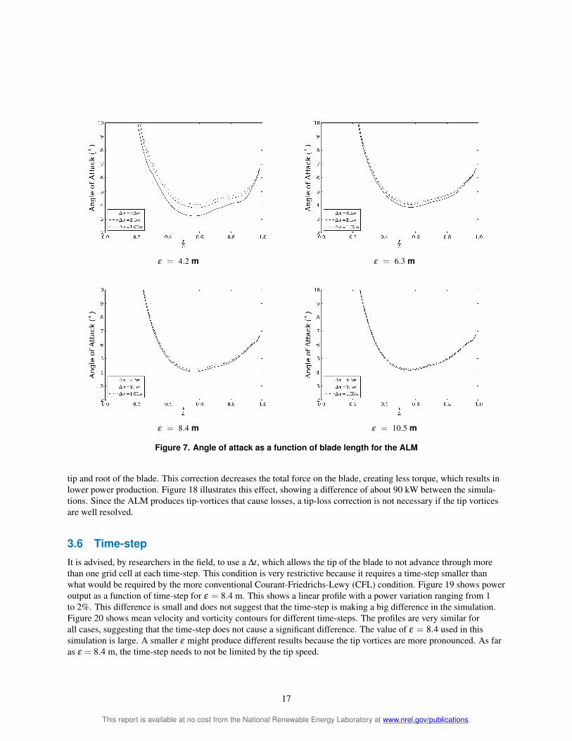
ε = 42 m ε = 63 m
ε = 84 m ε = 105 m
Figure 8 Axial velocity as a function of blade length for the ALM
37 Comparison
The ALM and ADM predict similar wake profiles and power output The main differences between the models are 1) the vortical structures near the rotor were captured by the ALM but not by the ADM and 2) a non-symmetric wake was observed with respect to the center-line with the ALM as opposed to the symmetric wake that was obshyserved in the ADM The ALM is able to capture vortical structures that are caused by the presence of individual blades Tip and root vortices are captured when using the ALM with a high enough grid resolution as seen in Figure 14 when ε = 42 m However the ADM does not allow these structures to form only the shear layer of the wake forms
Table 1 compares power output for the ADM ALM and BEM theory A Richardson extrapolation is used to elimishynate the leading error and predict the grid-converged power solution for the ADM and ALM The power has a similar behavior for the ADM and ALM As ε becomes smaller the power output for the ADM and ALM approaches what the BEM theory predicts Both models provide similar results but as ε becomes smaller the differences are bigger
In terms of computational costs the ALM needs to rotate the blades every time-step and thus apply forces at difshyferent finite-volume cells every time-step A search for these cells is performed every time-step The ADM points are fixed and do not rotate every time-step All the cells that lie adjacent to the disk are assigned at the beginning of the simulation thus all the finite-volume cells that have an applied force are searched for only once The ADM by
18
This report is available at no cost from the National Renewable Energy Laboratory at wwwnrelgovpublications
ALM ADM
ε = 42 m
ε = 63 m
ε = 84 m
ε = 105 m
Figure 9 Mean velocity in the cross-stream direction that is 1 diameter behind the turbine rotor are shown as predicted by the ALM (left column) and ADM (right column) Each row
shows plots that are the result of using different values of the body force projection width (ε)
19
This report is available at no cost from the National Renewable Energy Laboratory at wwwnrelgovpublications
ALM ADM
ε = 42 m
ε = 63 m
ε = 84 m
ε = 105 m
Figure 10 Mean velocity in the cross-stream direction that is 4 diameters behind the turbine rotor are shown as predicted by the ALM (left column) and ADM (right column) Each row
shows plots that are the result of using different values of the body force projection width (ε)
20
This report is available at no cost from the National Renewable Energy Laboratory at wwwnrelgovpublications
ALM ADM
ε = 42 m
ε = 63 m
ε = 84 m
ε = 105 m
Figure 11 Mean velocity (ms) contours in a plane through the turbine hub are shown as predicted by the ALM (left column) and ADM (right column) with a mesh resolution of Δx = 42 m Each row shows contours that are the result of using different values of the body force projection width (ε)
Table 1 Percentage difference between the ADM ALM and BEM theory in terms of power producshytion A Richardson extrapolation is used to approximate the converged solution for the ALM and ADM
Case Predicted Power (MW) Percentage Difference with BEM ALM ADM ALM ADM
ε = 21 m 181 -60 ε = 42 m 213 214 106 110 ε = 63 m 219 219 137 137 ε = 84 m 223 223 157 157
ε = 105 m 227 227 179 179
21
This report is available at no cost from the National Renewable Energy Laboratory at wwwnrelgovpublications
ALM ADM
ε = 42 m
ε = 63 m
ε = 84 m
ε = 105 m
Figure 12 Vorticity magnitude (1s) contours in a plane through the turbine hub are shown as preshydicted by the ALM (left column) and ADM (right column) with a mesh resolution of Δx = 42 m Each
row shows contours that are the result of using different values of the body force projection width (ε)
22
This report is available at no cost from the National Renewable Energy Laboratory at wwwnrelgovpublications
ALM ADM
ε = 42 m
ε = 63 m
ε = 84 m
ε = 105 m
Figure 13 Mean velocity (ms) contours in a plane through the turbine hub are shown as predicted by the ALM (left column) and ADM (right column) with a mesh resolution of Δx = 21 m Each row shows contours that are the result of using different values of the body force projection width (ε)
23
This report is available at no cost from the National Renewable Energy Laboratory at wwwnrelgovpublications
ALM ADM
ε = 42 m
ε = 63 m
ε = 84 m
ε = 105 m
Figure 14 Vorticity magnitude (1s) contours in a plane through the turbine hub are shown as preshydicted by the ALM (left column) and ADM (right column) with a mesh resolution of Δx = 21 m Each
row shows contours that are the result of using different values of the body force projection width (ε)
24
This report is available at no cost from the National Renewable Energy Laboratory at wwwnrelgovpublications
ALM ADM
ε = 42 m
ε = 63 m
ε = 84 m
ε = 105 m
Figure 15 Mean velocity (ms) contours in a plane through the turbine hub are shown as predicted by the ALM (left column) and ADM (right column) with a mesh resolution of Δx = 105 m Each row shows contours that are the result of using different values of the body force projection width (ε)
25
This report is available at no cost from the National Renewable Energy Laboratory at wwwnrelgovpublications
ALM ADM
ε = 42 m
ε = 63 m
ε = 84 m
ε = 105 m
Figure 16 Vorticity magnitude (1s) contours in a plane through the turbine hub are shown as preshydicted by the ALM (left column) and ADM (right column) with a mesh resolution of Δx = 105 m Each row shows contours that are the result of using different values of the body force projection width (ε)
26
This report is available at no cost from the National Renewable Energy Laboratory at wwwnrelgovpublications
Figure 17 Power output for the ALM as a function of actuator point resshyolution along the blade with ε = 84 and a grid resolution of 21 m
Figure 18 Power output as a function of grid resolution for ε = 84 m with and without a tip- and root-loss correction for the ALM
contrast has more points than the ALM and the forces on these points must be calculated for every time-step These differences do not impact the simulation time significantly However time-step size will have a significant impact on simulation time The time-step for simulations performed using the ALM is restricted by the tip speed The tip
27
This report is available at no cost from the National Renewable Energy Laboratory at wwwnrelgovpublications
Figure 19 Power output as a function of time-step for ε = 84 m
of the blade should not pass through more than a single finite-volume cell each time-step This condition is far more restrictive than the typical CFL condition For a case with λ =8 the time-step needs to be eight times smaller using this restriction than with the CFL condition Resolving the root- and tip-vortices compromises the simulation time-step and thus increases computational cost The ADM will provide an accurate solution with a time-step that is based on a CFL condition rather than on tip speed If the simulations require solving the flow structures near the rotor the ALM should be used For simulations related to the far wake the ADM will provide a reasonable solution without compromising the simulation time-step
38 The ε Parameter
A Gaussian function is introduced to turn the set of unphysical point forces into a continuous volume force field The use of a Gaussian function avoids numerical instabilities caused by the application of forces on discrete sections of the blade The width of the function is determined by the ε parameter This parameter plays an important role in the models studied We found that a parameter closest to the characteristic length of the blade section under study yielded the best results The value of the Gaussian function decays to 1 of its initial value at a distance of r = 215ε To span the force of a blade section through the area that covers the distance from the leading edge to the trailing edge a value of ε = c43 would be required With a chord value around 4 m for the NREL 5-MW turbine a value of ε = 4 m43 = 093 m creates numerical instabilities on the grids used in this study Our projections show that making the grid smaller would be expensive unless a fine grid local to the rotor was used
The simulations presented show that as ε becomes smaller the power decreases Note that a small value of ε relashytive to the grid size produces numerical instabilities in the solver These instabilities affect the solution and can be observed in the wake profiles and angle of attack for a case in which ε = 42 m and a grid resolution of 42 m When parameter ε was the same size as the grid size (εΔx = 1) the simulations for the ALM and ADM became unstable This can be avoided by choosing a value of εΔx gt 2 as suggested by Troldborg [9] There is an optimum point for the Gaussian width to match what the BEM theory predicts This optimum is related to the geometry of the blade In this case the solution given by the BEM theory lies somewhere between ε =42 and 21 m It is unclear which value of ε matches the geometry of the blade section and would accurately predict power using the ALM The results
28
This report is available at no cost from the National Renewable Energy Laboratory at wwwnrelgovpublications
Vorticity Mean Velocity
Δt = 0015s
Δt = 003s
Δt = 006s
Δt = 01s
Figure 20 Mean velocity (ms) and vorticity magnitude (1s) contours in a plane through the turbine hub for ε = 84 m are shown Each row shows contours that are the result of using different time-step values
29
This report is available at no cost from the National Renewable Energy Laboratory at wwwnrelgovpublications
suggest that the value of ε should not be fixed to a value that satisfies the condition that ε = c43 A condition that better approximates the physical force distribution of an airfoil should be used varying ε along the span as the chord varies
Increasing the value of ε thickens the shear layer surrounding the wake As the shear layer is thickened there is less vorticity in the flow This is illustrated in Figures 12 14 and 16 as the vorticity decreases with larger ε
30
This report is available at no cost from the National Renewable Energy Laboratory at wwwnrelgovpublications
4 Wind Tunnel Simulations
We have performed a validation of the actuator line model (ALM) that compares the numerical results with the experiments done at the low-speed closed-return wind tunnel at the Department of Energy and Process Engineering at the Norwegian University of Science and Technology Trondheim [26][27] The tunnel has a test section of 185 meters (m) (height) times 271 m (width) times 1115 m (length) The test section height is adjustable to account for wall boundary layer growth In this study we aimed to numerically simulate the experimental setup
We performed simulations for tip speed ratios (λ ) of 3 4 6 9 and 12 and compared the power and thrust coefshyficients against the experimental data In addition we used wake visualizations to illustrate the difference in the breakdown of the wake for different tip speed ratios as well as sampled wake profiles
41 Turbine Model
The turbine modeled has a rotor with a diameter of 0894 m and a tower with a height of 0817 m The blades use the National Renewable Energy Laboratory (NREL) S826 airfoil along the entire span We obtained two-dimensional lift and drag coefficients from the NREL S826 report [28] and corrected for stall delay using NRELrsquos AirfoilPrep tool [29] The actuator line model accounts for only the blades of the turbine and does not include the hub tower or nacelle The turbine is located 366 m from the tunnel inlet and is laterally centered
42 Mesh
The mesh of the tunnel consists of a block with dimensions (1115 m times 1851 m times 271 m) The walls are refined in an attempt to capture the boundary layer The height of the tunnel varies linearly along the streamwise direction from 1801 m to 1851 m The mesh is refined near the walls to capture the boundary layer The walls have a no-slip condition The grid resolution near the wall does not resolve the boundary layer completely but because the rotor is far from the walls we believe the effect of not resolving this boundary layer is negligible The mesh is locally refined near the rotor with ΔxD = 0006 This refinement allows the simulation to calculate power production accurately (following the results from the previous section)
The boundary layer is measured to be 01 m at the tunnel inlet The inlet bulk velocity is taken to be 10 meters per second (ms) The inlet boundary condition is set to match the turbulent boundary layer profile using y 17
U = (41)δ
At y gt δ the velocity is set to 10 ms with no turbulence
43 Results
Power and thrust coefficients are shown as a function of tip speed ratio in Figure 21 The maximum power coeffishycient of 047 is at a tip speed ratio of 6 This corresponds to the highest induction factor as we expected For the case with lowest tip speed ratio the simulation power coefficient lies on top of the experimental data Thrust coefficient is under-predicted for all tip speed ratios
Figure 22 shows wake profiles in the spanwise direction for 1 2 3 and 4 diameters behind the rotor The profiles show how the wake deficit is stronger for higher tip speed ratios Note that for stronger wake deficits the velocity near the edges and in the center of the rotor is larger because of mass conservation Figure 23 shows wake profiles for cases with tip speed ratios of 3 and 6 that are one diameter behind the rotor The wakes in the simulation are different from the experimental data at the center This difference is because the nacelle is not a part of the model It is clear that the nacelle needs to be incorporated into the model to obtain accurate wake profiles As a result this
31
This report is available at no cost from the National Renewable Energy Laboratory at wwwnrelgovpublications
difference causes the thrust to be lower than expected because the nacelle will contribute a drag force to the model For this reason the thrust coefficient curve for the simulations lies below the experimental data Away from the center the wake profiles agree with the experimental data
Figure 24 shows a rendering of the Q-criterion [30] for tip speed ratios of λ = 3 6 9 and 12 The Q-criterion is the second invariant of the velocity gradient tensor Where it is positive it shows regions of the flow where rotation dominates strain and where it is negative strain dominates rotation This illustrates that the breakdown of the wake is faster with increased tip speed ratio With higher tip speed ratio the wake deficit is greater as shown in Figure 22 indicating there is a stronger more unstable wake-edge shear layer This causes faster transition to turbulence and faster wake breakdown The visualizations show that at higher tip speeds the wake starts interacting with the tunnel walls This interaction affects the wake as it is not able to fully expand
The ALM is a good representation of the turbine in the tunnel but is missing some key elements in its implementashytion The model is able to capture the blades inside the flow field Because the power of the turbine is being extracted by the blades the power coefficient is close to what experiments predict However the effect of the nacelle is not included in the model The nacelle contributes to the thrust experienced by the turbine and for this reason the thrust coefficient is under-predicted by the model Tip speed ratio affects the power produced by the turbine and the strucshyture of the wake The maximum power coefficient is reached at a tip speed ratio of 6 which approximates the Betz limit A faster tip speed ratio causes a faster breakdown of the wake
Power Thrust
Figure 21 Power and thrust coefficients as a function of tip speed ratio
32
This report is available at no cost from the National Renewable Energy Laboratory at wwwnrelgovpublications
xD = 1 xD = 2
xD = 3 xD = 4
Figure 22 Mean velocity profiles behind the rotor
33
This report is available at no cost from the National Renewable Energy Laboratory at wwwnrelgovpublications
1D TSR=3 1D TSR=6
3D TSR=3 3D TSR=6
Figure 23 Mean velocity profiles one and three diameters behind the rotor
34
This report is available at no cost from the National Renewable Energy Laboratory at wwwnrelgovpublications
λ = 3 λ = 6
λ = 9 λ = 12
Figure 24 Q-criterion (1s2) rendering showing the structure of the wake for different tip speed ratios
35
This report is available at no cost from the National Renewable Energy Laboratory at wwwnrelgovpublications
5 Wind Farm Simulation
51 Introduction
This section presents the results of a large-eddy simulation (LES) of the flow of over 48 multi-megawatt turbines that compose the Lillgrund wind plant We compared the performance of the actuator line (ALM) and actuator disk model (ADM) in wind farm simulations Churchfield et al [31] performed an LES of the Lillgrund wind farm using the ALM we performed the same simulation using the ADM and compared the results for both models The simulated wind farm is the Lillgrund offshore facility operated by Vattenfall Vindkraft AB Lillgrund is located 7 kilometers (km) off the coast of Sweden and 7 km south of the Oumlresund bridge Figure 25 shows the turbine siting and the computational domain Positive x and y correspond to east and north respectively
We used LES to simulate the atmospheric boundary layer (ABL) with the standard Smagorinsky model We modeled the sea surface as a rough flat surface with an aerodynamic roughness height of 01 millimiters (mm) which was appropriate for the sea surface The turbine model operating at the Lillgrund facility is the Siemens SWT-23-93 The turbine model was provided by Churchfield who reverse-engineered the available turbine information [32] We performed the simulation in two steps running an ABL precursor simulation and running the wind plant simulation The first precursor simulation tried to match the Lillgrund wind conditions as closely as possible and was obtained from Churchfield [31] We chose a mean velocity of 9 ms at hub-height with a wind direction of 2216o At these conditions the turbines operating in Region 2 wake deficits are the strongest We used the turbulent intensity at hub-height of 62 which is typical at the chosen wind direction The precursor simulation was used to create a turbulent wind inlet (west and south) boundary condition on velocity and temperature for the simulation The east and north planes were set to zero gradient for velocity and temperature The velocity top boundary condition was set to zero in the normal direction and to zero gradient in the other two directions The pressure boundary conditions were set to hydrostatic gradient on the top and bottom and to zero gradient on the sides The temperature gradient on the top was set to 0003 Kelvins per meter (Km) to follow the temperature profile in capping inversion The precursor simulation was the same for both the ADM and ALM simulation The time-step of the ALM simulation was fixed at the condition that the tip of the blade should not go through more than one grid cell at each time-step The time-step in the ADM simulation was based on the maximum Courant number not exceeding a limit of 075 The wind plant simulation was for 10 minutes of real time and an initial transient of 150 s
52 Results
Normalized power output is shown for all the rows in the turbine array in Figure 26 Rows B through D are comshypared against field data that were averaged over a year and binned by wind direction Power output for these rows is normalized using the average power of the first turbine in rows B C and D The other turbines are normalized using the power of the first turbine in their row The simulations agree with field data The largest difference is on the last turbines in the rows where the simulation predicted an increase in power production Figure 27 shows non-normalized power output for all the turbines Power production for the ADM agrees well with that for ALM although we observe slight differences The percent difference between the ADM and ALM dimensional power flucshytuated between 1 and 17 Contrasting what we observed in Chapter 3 the ALM produces a slightly higher power output than the ADM The power curve for the model predicts 1347 megawatts (MW) at 9 ms The first turbine in each row is close to this value for both the ADM and ALM although we observed that the ALM usually over predicts power whereas the ADM under predicts power
Figure 28 shows the mean velocity profiles for the ADM and ALM The wake deficits in the ADM simulation are stronger (shown in dark blue) than the ALM Figure 29 shows the difference between the ADM and ALM simulashytions which was calculated by subtracting the ADM data from the ALM data The figure reveals that the regions near the center of the wake have the strongest difference (shown in red)
Figure 30 shows wake profiles along rows C and E The profiles pass through the hub and outboard of the hub in increments of D8 where D is the rotor diameter This shows the wake differences between the models at several
36
This report is available at no cost from the National Renewable Energy Laboratory at wwwnrelgovpublications
Figure 25 Wind farm layout (left) and computational doshymain (right) Illustration by Matthew J Churchfield NREL
locations The biggest difference in wake profiles is on the wake of the first turbine in each row The ADM creates a larger velocity deficit in the center when passing through the first turbine The flow begins to recover in the far wake before hitting the next turbines The ALM and ADM recover to nearly the same value This pattern repeats until the last turbine in the row There is a gap in row E where the flow recovers more than the rest of the turbines This recovery produces more power on the next turbine in the row although the flow is not fully recovered A power production difference of 30 was observed between the turbine right after the gap and the subsequent one The wake recovery in the gap allows greater power production from the next turbine in the row Field data always show a slight increase in power of the third turbine over the second turbine in the row The ALM does not predict this but the ADM does
Figures 32 33 and 34 show wake profiles for turbines 27 through 30 and at 05 075 and 1 diameter behind the rotor The profiles show that the velocity deficit near the center of the wake for the ADM is stronger than that of the ALM However moving towards the edge of the wake the velocity deficit from the ALM is stronger than for the ADM
The time-step used for the ALM simulation was Δt =0015 s while the time-step for the ADM simulation was based on a Courant-Friedrichs-Lewy number of 075 with typical values close to Δt =006 s The difference in time-step may cause the power output differences that were observed Figure 19 shows that as Δt increases predicted power decreases similar to what Figure 27 shows
The ADM simulation was completed two times faster than the ALM simulation The ALM simulation required about 1 million CPU-hours whereas the ADM showed significant savings This difference is because the ADM has a higher time-step On a time per time-step basis the ADM takes longer to calculate all the body forces on the disk (rather than just the body forces on the blades of the ALM)
The ALM and ADM provide similar results in large-scale wind farm simulations There is a difference in power production in which the ALM produces more power than the ADM The difference in the first row of turbines is larger than the turbines that are further downstream In terms of computational cost the ADM can be run faster because time-step is not limited to tip speed The ADM simulation was completed three times faster than the ALM This time reduction is crucial when performing these type of simulations The wake in the ADM has a greater deficit
37
This report is available at no cost from the National Renewable Energy Laboratory at wwwnrelgovpublications
in the center than the ALM However the velocity deficit near the edges is stronger for the ALM indicating a larger power extraction is near the outer portion of the blades The total difference shows that the power extraction for the ALM is greater than that for the ADM
38
This report is available at no cost from the National Renewable Energy Laboratory at wwwnrelgovpublications
Row A Row B
Row C Row D
Row E Row F
Row G Row H
macrFigure 26 Ten minute average power produced by each turbine Pi normalized by the power of the first turbine in the row Average over one year of field data is shown for rows B-D
39
This report is available at no cost from the National Renewable Energy Laboratory at wwwnrelgovpublications
Row A Row B
Row C Row D
Row E Row F
Row G Row H
Figure 27 Power produced by each turbine
40
This report is available at no cost from the National Renewable Energy Laboratory at wwwnrelgovpublications
ADM ALM
Figure 28 Mean velocity (ms) contours at hub height for ADM (left) and ALM (right)
Figure 29 Mean velocity difference (ms) between ALM and ADM (ALM-ADM)
41
This report is available at no cost from the National Renewable Energy Laboratory at wwwnrelgovpublications
Row C Row E
yR = 0
yR = 025
yR = 05
yR = 075
yR = 1
Figure 30 Mean streamwise velocity profiles at hub height along rows C and E at various horizontal locations outboard of hub ranging from hub to blade tip
Turbine 30 Turbine 29
Turbine 28 Turbine 27
Figure 31 Mean velocity in the cross stream direction at one-fourth diameter behind the rotor for turbines in row D
42
This report is available at no cost from the National Renewable Energy Laboratory at wwwnrelgovpublications
Turbine 30 Turbine 29
Turbine 28 Turbine 27
Figure 32 Mean velocity in the cross stream direction at one-half diameter behind the rotor for turbines in row D
Turbine 30 Turbine 29
Turbine 28 Turbine 27
Figure 33 Mean velocity in the cross stream direction at three-fourths diameter behind the rotor for turbines in row D
43
This report is available at no cost from the National Renewable Energy Laboratory at wwwnrelgovpublications
Turbine 30 Turbine 29
Turbine 28 Turbine 27
Figure 34 Mean velocity in the cross stream direction at 1 diameter behind the rotor for turbines in row D
Turbine 30 Turbine 29
Turbine 28 Turbine 27
Figure 35 Mean velocity in the cross stream direction at 3 diameters behind the rotor for turbines in row D
44
This report is available at no cost from the National Renewable Energy Laboratory at wwwnrelgovpublications
Turbine 30 Turbine 29
Turbine 28 Turbine 27
Figure 36 Mean velocity in the cross stream direction at 4 diameters behind the rotor for turbines in row D
45
This report is available at no cost from the National Renewable Energy Laboratory at wwwnrelgovpublications
6 Conclusion and Future Work
The actuator line model (ALM) and actuator disk model (ADM) are a suitable representation of a wind turbine when using numerical simulations of fluid flows The models do not require that the full geometry of the blades be resolved and in which case model them as a set of points in the flow The ALM models the blades as a set of points along each blade axis whereas the ADM models the rotor as a disk with points that represent sections of the disk
The ADM and ALM provide very similar results in simulations with uniform inflow There is a clear grid depenshydence on power production and wake profiles of the ADM and ALM As the grid is refined the predicted power increases for both models Using a Glauert tip-loss correction with the ALM decreases the power production The number of actuator points in the ALM should be adequate to account for all the sections of the blade and provide smooth changes between them We recommend using a value smaller than ΔbΔx = 075 Mean wake profiles are similar for both the ADM and ALM
A Gaussian function was introduced to avoid numerical instabilities that are caused by the application of forces on discrete sections of the blade The width of the function was determined by the ε parameter This parameter played an important role in the models studied We observed that a parameter closest to the characteristic length of the blade section yielded the best results As the width of the projection function is decreased both the ALM and ADM predicted power decreases but never converges upon a value A specific value of epsilon allows agreement with blade-element momentum theory predictions However the ε parameter must be higher than 2Δx to avoid numerical instabilities in the solver
The ALM resolves the flow structures that are caused by the presence of individual blades which the ADM does not The ALM matches the physics more closely because it captures the root- and tip-vortices which the ADM does not Also the ALM is able to capture helical and asymmetric structures across the wake which caused asymmetric roll-up of Kelvin-Helmholtz-like instabilities in the wakersquos outer shear layer The ALM captures the vortical structures in the near wake ADM provides good results in the far wake but does not produce the vortical structures near the rotor If simulations are intended to determine the far wake effects the ADM should provide reasonable results
We used the ALM to validate a small-scale wind tunnel experiment and compared the structure of the wake for different tip speed ratios We observed that as the tip speed ratio is higher the breakdown of the wake occurs faster leaving a wider wake for larger tip speed ratios The tunnel walls play an important role in the simulation as the wake interacts with the walls The blockage effect of the turbine makes the reference velocity of the tunnel higher near the rotor than on the inlet
When performing large-scale wind farm simulations we found that the models perform well ALM produces slightly more power than ADM under atmospheric boundary layer conditions It is still unknown why this occurs but it is possible that the difference is caused by the time-step difference in the simulations The wake of the ADM is different from that of the ALM The ADM wake has a stronger wake deficit near the center whereas the ALM has a stronger wake deficit near the edges Wake profiles are similar but we observed that the greatest difference in the near wake primarily in the first row of turbines
46
This report is available at no cost from the National Renewable Energy Laboratory at wwwnrelgovpublications
Bibliography
[1] JN Soslashrensen Aerodynamics aspects of wind energy conversion 43427ndash448 September 2010
[2] T Burton D Sharpe N Jenkins and E Bossanyi Aerodynamics of Horizontal-Axis Wind Turbines pages 41ndash172 John Wiley amp Sons Ltd 2002
[3] JF Manwell JG McGowan and AL Rogers Wind Energy Explained Theory Design and Application Wiley 2010
[4] B Sanderse SP van der Pijl and B Koren Review of computational fluid dynamics for wind turbine wake aerodynamics Wind Energy 14 2011
[5] F Porteacute-Agel H Lu and YT Wu A Large-Eddy simulation framework for wind energy applications The Fifth International Symposium on Computational Wind Engineering (CWE2010) Chapel Hill North Carolina USA May 23-27 2010
[6] M Calaf C Meneveau and J Meyers Large eddy simulation study of fully developed wind-turbine array boundary layers Physics of Fluids 22(1)015110 2010
[7] N Troldborg JN Soslashrensen and R Mikkelsen Numerical simulations of wake charasteristics of a wind turbine in uniform flow 1386ndash99 2009
[8] T Phuoc Aeacuterodynamique instationnaire turbulente - aspects numeacuteriques et expeacuterimentaux Journeacute theacutematique DRET 1994
[9] N Troldborg Actuator Line Modeling of Wind Turbine Wakes PhD thesis Technical University of Denmark Lyngby Denmark 2008
[10] I Ammara C Leclerc and C Masson A viscous three-dimensional differentialactuator-disk method for the aerodynamic analysis of wind farms Journal of Solar Energy Engineering 124(4)345ndash356 2002
[11] A Jimenez A Crespo E Migoya and J Garcia Advances in large-eddy simulation of a wind turbine wake Journal of Physics Conference Series 75(1)012041 2007
[12] C Masson A Smaiumlli and C Leclerc Aerodynamic analysis of hawts operating in unsteady conditions Wind Energy 4(1)1ndash22 2001
[13] R Mikkelsen JN Soslashrensen and WZ Shen Modelling and analysis of the flow field around a coned rotor Wind Energy 4(3)121ndash135 2001
[14] JN Soslashrensen and WZ Shen Numerical modeling of wind turbine wakes Journal of Fluids Engineering 124(2)393ndash399 June 2002
[15] SSA Ivanell JN Soslashrensen R Mikkelsen and D Henningson Analysis of numerically generated wake structures Wind Energy 12(1)63ndash80 2009
[16] R Mikkelsen JN Soslashrensen S Oslashye and N Troldborg Analysis of power enhancement for a row of wind turbines using the actuator line technique Journal of Physics Conference Series ndash The Science of Making Torque from Wind 75(012044) 2007
[17] R Mikkelsen Actuator Disc Methods Applied to Wind Turbines PhD thesis Technical University of Denmark Mechanical Engineering Department 2003
[18] WZ Shen JH Zhang and JN Soslashrensen The actuator surface model A new navierndashstokes based model for rotor computations Journal of Solar Energy Engineering 131(1)011002 2009
47
This report is available at no cost from the National Renewable Energy Laboratory at wwwnrelgovpublications
[19] I Dobrev F Massouh and M Rapin Actuator surface hybrid model Journal of Physics Conference Series 75(1)012019 2007
[20] CS Watters and C Masson Modeling of lifting-device aerodynamics using the actuator surface concept International Journal for Numerical Methods in Fluids 62(11)1264ndash1298 2010
[21] OpenFOAM Ver 171 [available online] Silicon Graphics International Corporation (SGI) URL httpwwwopenfoamorgarchive171download [accessed 13 December 2011]
[22] J Smagorinsky General circulation experiments with the primitive equations Monthly Weather Review 9199ndash164 1963
[23] MJ Buhl WT_Perf Userrsquos Guide National Renewable Energy Laboratory 2004
[24] H Glauert Airplane Propellers pages 251ndash268 Dover New York 1985
[25] J Jonkman S Butterfield W Musial and G Scott Definition of a 5-MW reference wind turbine for offshore system development Technical Report NRELTP-500-38060
[26] MS Adaramola and P-A Krogstad Experimental investigation of wake effects on wind turbine performance Renewable Energy 362078ndash2086 2011
[27] P-A Krogstad and JA Lund An experimental and numerical study of the performance of a model turbine Wind Energy 2011
[28] DM Somers The S825 and S826 Airfoils Period of Performance 1994ndash1995 The S825 and S826 Airfoils Technical Report January 2005
[29] NWTC Design Codes (AirfoilPrep by Dr Craig Hansen) httpwindnrelgovdesigncodespreprocessorsairfoilprep [Accessed 21 February 2012]
[30] JCR Hunt AA Wray and P Moin Eddies streams and convergence zones in turbulent flows (1970) 1988
[31] MJ Churchfield S Lee P Moriarty LA Martiacutenez S Leonardi G Vijayakumar and JG Brasseur A large-eddy simulation of wind-plant aerodynamics 50th AIAA Aerospace Sciences Meeting Nashville Tennessee USA 2012
[32] MJ Churchield A Method for Designing Generic Wind Turbine Models Representative of Real Turbines and Generic Siemens SWT-23-93 and Vestas V80 Specifications National Renewable Energy Laboratory 2012
48
This report is available at no cost from the National Renewable Energy Laboratory at wwwnrelgovpublications
- Literature Review
-
- Introduction
- Basics of Wind Turbine Aerodynamics
- Wind Turbine Computational Fluid Dynamics
- Atmospheric Boundary Layer Simulations
- Actuator Disc Model (ADM)
- Actuator Line Model (ALM)
- Actuator Surface Model (ASM)
- Comparison Between ADM and ALM
- Conclusions
-
- Actuator Turbine Model Implementation
-
- Actuator Line Model
- Actuator Disk Model
- Numerical Method
-
- Actuator Disk and Actuator Line Models in Uniform Nonturbulent Inflow
-
- Five Megawatt Reference Turbine
- Actuator Line Model
- Actuator Disk Model
- Actuator Points
- Tip Loss Correction
- Time-step
- Comparison
- The Parameter
-
- Wind Tunnel Simulations
-
- Turbine Model
- Mesh
- Results
-
- Wind Farm Simulation
-
- Introduction
- Results
-
- Conclusion and Future Work
- Bibliography
-
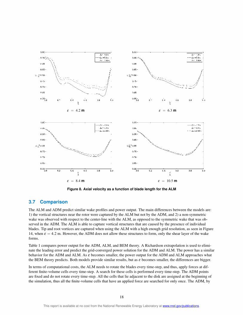
ALM ADM
ε = 42 m
ε = 63 m
ε = 84 m
ε = 105 m
Figure 13 Mean velocity (ms) contours in a plane through the turbine hub are shown as predicted by the ALM (left column) and ADM (right column) with a mesh resolution of Δx = 21 m Each row shows contours that are the result of using different values of the body force projection width (ε)
23
This report is available at no cost from the National Renewable Energy Laboratory at wwwnrelgovpublications
ALM ADM
ε = 42 m
ε = 63 m
ε = 84 m
ε = 105 m
Figure 14 Vorticity magnitude (1s) contours in a plane through the turbine hub are shown as preshydicted by the ALM (left column) and ADM (right column) with a mesh resolution of Δx = 21 m Each
row shows contours that are the result of using different values of the body force projection width (ε)
24
This report is available at no cost from the National Renewable Energy Laboratory at wwwnrelgovpublications
ALM ADM
ε = 42 m
ε = 63 m
ε = 84 m
ε = 105 m
Figure 15 Mean velocity (ms) contours in a plane through the turbine hub are shown as predicted by the ALM (left column) and ADM (right column) with a mesh resolution of Δx = 105 m Each row shows contours that are the result of using different values of the body force projection width (ε)
25
This report is available at no cost from the National Renewable Energy Laboratory at wwwnrelgovpublications
ALM ADM
ε = 42 m
ε = 63 m
ε = 84 m
ε = 105 m
Figure 16 Vorticity magnitude (1s) contours in a plane through the turbine hub are shown as preshydicted by the ALM (left column) and ADM (right column) with a mesh resolution of Δx = 105 m Each row shows contours that are the result of using different values of the body force projection width (ε)
26
This report is available at no cost from the National Renewable Energy Laboratory at wwwnrelgovpublications
Figure 17 Power output for the ALM as a function of actuator point resshyolution along the blade with ε = 84 and a grid resolution of 21 m
Figure 18 Power output as a function of grid resolution for ε = 84 m with and without a tip- and root-loss correction for the ALM
contrast has more points than the ALM and the forces on these points must be calculated for every time-step These differences do not impact the simulation time significantly However time-step size will have a significant impact on simulation time The time-step for simulations performed using the ALM is restricted by the tip speed The tip
27
This report is available at no cost from the National Renewable Energy Laboratory at wwwnrelgovpublications
Figure 19 Power output as a function of time-step for ε = 84 m
of the blade should not pass through more than a single finite-volume cell each time-step This condition is far more restrictive than the typical CFL condition For a case with λ =8 the time-step needs to be eight times smaller using this restriction than with the CFL condition Resolving the root- and tip-vortices compromises the simulation time-step and thus increases computational cost The ADM will provide an accurate solution with a time-step that is based on a CFL condition rather than on tip speed If the simulations require solving the flow structures near the rotor the ALM should be used For simulations related to the far wake the ADM will provide a reasonable solution without compromising the simulation time-step
38 The ε Parameter
A Gaussian function is introduced to turn the set of unphysical point forces into a continuous volume force field The use of a Gaussian function avoids numerical instabilities caused by the application of forces on discrete sections of the blade The width of the function is determined by the ε parameter This parameter plays an important role in the models studied We found that a parameter closest to the characteristic length of the blade section under study yielded the best results The value of the Gaussian function decays to 1 of its initial value at a distance of r = 215ε To span the force of a blade section through the area that covers the distance from the leading edge to the trailing edge a value of ε = c43 would be required With a chord value around 4 m for the NREL 5-MW turbine a value of ε = 4 m43 = 093 m creates numerical instabilities on the grids used in this study Our projections show that making the grid smaller would be expensive unless a fine grid local to the rotor was used
The simulations presented show that as ε becomes smaller the power decreases Note that a small value of ε relashytive to the grid size produces numerical instabilities in the solver These instabilities affect the solution and can be observed in the wake profiles and angle of attack for a case in which ε = 42 m and a grid resolution of 42 m When parameter ε was the same size as the grid size (εΔx = 1) the simulations for the ALM and ADM became unstable This can be avoided by choosing a value of εΔx gt 2 as suggested by Troldborg [9] There is an optimum point for the Gaussian width to match what the BEM theory predicts This optimum is related to the geometry of the blade In this case the solution given by the BEM theory lies somewhere between ε =42 and 21 m It is unclear which value of ε matches the geometry of the blade section and would accurately predict power using the ALM The results
28
This report is available at no cost from the National Renewable Energy Laboratory at wwwnrelgovpublications
Vorticity Mean Velocity
Δt = 0015s
Δt = 003s
Δt = 006s
Δt = 01s
Figure 20 Mean velocity (ms) and vorticity magnitude (1s) contours in a plane through the turbine hub for ε = 84 m are shown Each row shows contours that are the result of using different time-step values
29
This report is available at no cost from the National Renewable Energy Laboratory at wwwnrelgovpublications
suggest that the value of ε should not be fixed to a value that satisfies the condition that ε = c43 A condition that better approximates the physical force distribution of an airfoil should be used varying ε along the span as the chord varies
Increasing the value of ε thickens the shear layer surrounding the wake As the shear layer is thickened there is less vorticity in the flow This is illustrated in Figures 12 14 and 16 as the vorticity decreases with larger ε
30
This report is available at no cost from the National Renewable Energy Laboratory at wwwnrelgovpublications
4 Wind Tunnel Simulations
We have performed a validation of the actuator line model (ALM) that compares the numerical results with the experiments done at the low-speed closed-return wind tunnel at the Department of Energy and Process Engineering at the Norwegian University of Science and Technology Trondheim [26][27] The tunnel has a test section of 185 meters (m) (height) times 271 m (width) times 1115 m (length) The test section height is adjustable to account for wall boundary layer growth In this study we aimed to numerically simulate the experimental setup
We performed simulations for tip speed ratios (λ ) of 3 4 6 9 and 12 and compared the power and thrust coefshyficients against the experimental data In addition we used wake visualizations to illustrate the difference in the breakdown of the wake for different tip speed ratios as well as sampled wake profiles
41 Turbine Model
The turbine modeled has a rotor with a diameter of 0894 m and a tower with a height of 0817 m The blades use the National Renewable Energy Laboratory (NREL) S826 airfoil along the entire span We obtained two-dimensional lift and drag coefficients from the NREL S826 report [28] and corrected for stall delay using NRELrsquos AirfoilPrep tool [29] The actuator line model accounts for only the blades of the turbine and does not include the hub tower or nacelle The turbine is located 366 m from the tunnel inlet and is laterally centered
42 Mesh
The mesh of the tunnel consists of a block with dimensions (1115 m times 1851 m times 271 m) The walls are refined in an attempt to capture the boundary layer The height of the tunnel varies linearly along the streamwise direction from 1801 m to 1851 m The mesh is refined near the walls to capture the boundary layer The walls have a no-slip condition The grid resolution near the wall does not resolve the boundary layer completely but because the rotor is far from the walls we believe the effect of not resolving this boundary layer is negligible The mesh is locally refined near the rotor with ΔxD = 0006 This refinement allows the simulation to calculate power production accurately (following the results from the previous section)
The boundary layer is measured to be 01 m at the tunnel inlet The inlet bulk velocity is taken to be 10 meters per second (ms) The inlet boundary condition is set to match the turbulent boundary layer profile using y 17
U = (41)δ
At y gt δ the velocity is set to 10 ms with no turbulence
43 Results
Power and thrust coefficients are shown as a function of tip speed ratio in Figure 21 The maximum power coeffishycient of 047 is at a tip speed ratio of 6 This corresponds to the highest induction factor as we expected For the case with lowest tip speed ratio the simulation power coefficient lies on top of the experimental data Thrust coefficient is under-predicted for all tip speed ratios
Figure 22 shows wake profiles in the spanwise direction for 1 2 3 and 4 diameters behind the rotor The profiles show how the wake deficit is stronger for higher tip speed ratios Note that for stronger wake deficits the velocity near the edges and in the center of the rotor is larger because of mass conservation Figure 23 shows wake profiles for cases with tip speed ratios of 3 and 6 that are one diameter behind the rotor The wakes in the simulation are different from the experimental data at the center This difference is because the nacelle is not a part of the model It is clear that the nacelle needs to be incorporated into the model to obtain accurate wake profiles As a result this
31
This report is available at no cost from the National Renewable Energy Laboratory at wwwnrelgovpublications
difference causes the thrust to be lower than expected because the nacelle will contribute a drag force to the model For this reason the thrust coefficient curve for the simulations lies below the experimental data Away from the center the wake profiles agree with the experimental data
Figure 24 shows a rendering of the Q-criterion [30] for tip speed ratios of λ = 3 6 9 and 12 The Q-criterion is the second invariant of the velocity gradient tensor Where it is positive it shows regions of the flow where rotation dominates strain and where it is negative strain dominates rotation This illustrates that the breakdown of the wake is faster with increased tip speed ratio With higher tip speed ratio the wake deficit is greater as shown in Figure 22 indicating there is a stronger more unstable wake-edge shear layer This causes faster transition to turbulence and faster wake breakdown The visualizations show that at higher tip speeds the wake starts interacting with the tunnel walls This interaction affects the wake as it is not able to fully expand
The ALM is a good representation of the turbine in the tunnel but is missing some key elements in its implementashytion The model is able to capture the blades inside the flow field Because the power of the turbine is being extracted by the blades the power coefficient is close to what experiments predict However the effect of the nacelle is not included in the model The nacelle contributes to the thrust experienced by the turbine and for this reason the thrust coefficient is under-predicted by the model Tip speed ratio affects the power produced by the turbine and the strucshyture of the wake The maximum power coefficient is reached at a tip speed ratio of 6 which approximates the Betz limit A faster tip speed ratio causes a faster breakdown of the wake
Power Thrust
Figure 21 Power and thrust coefficients as a function of tip speed ratio
32
This report is available at no cost from the National Renewable Energy Laboratory at wwwnrelgovpublications
xD = 1 xD = 2
xD = 3 xD = 4
Figure 22 Mean velocity profiles behind the rotor
33
This report is available at no cost from the National Renewable Energy Laboratory at wwwnrelgovpublications
1D TSR=3 1D TSR=6
3D TSR=3 3D TSR=6
Figure 23 Mean velocity profiles one and three diameters behind the rotor
34
This report is available at no cost from the National Renewable Energy Laboratory at wwwnrelgovpublications
λ = 3 λ = 6
λ = 9 λ = 12
Figure 24 Q-criterion (1s2) rendering showing the structure of the wake for different tip speed ratios
35
This report is available at no cost from the National Renewable Energy Laboratory at wwwnrelgovpublications
5 Wind Farm Simulation
51 Introduction
This section presents the results of a large-eddy simulation (LES) of the flow of over 48 multi-megawatt turbines that compose the Lillgrund wind plant We compared the performance of the actuator line (ALM) and actuator disk model (ADM) in wind farm simulations Churchfield et al [31] performed an LES of the Lillgrund wind farm using the ALM we performed the same simulation using the ADM and compared the results for both models The simulated wind farm is the Lillgrund offshore facility operated by Vattenfall Vindkraft AB Lillgrund is located 7 kilometers (km) off the coast of Sweden and 7 km south of the Oumlresund bridge Figure 25 shows the turbine siting and the computational domain Positive x and y correspond to east and north respectively
We used LES to simulate the atmospheric boundary layer (ABL) with the standard Smagorinsky model We modeled the sea surface as a rough flat surface with an aerodynamic roughness height of 01 millimiters (mm) which was appropriate for the sea surface The turbine model operating at the Lillgrund facility is the Siemens SWT-23-93 The turbine model was provided by Churchfield who reverse-engineered the available turbine information [32] We performed the simulation in two steps running an ABL precursor simulation and running the wind plant simulation The first precursor simulation tried to match the Lillgrund wind conditions as closely as possible and was obtained from Churchfield [31] We chose a mean velocity of 9 ms at hub-height with a wind direction of 2216o At these conditions the turbines operating in Region 2 wake deficits are the strongest We used the turbulent intensity at hub-height of 62 which is typical at the chosen wind direction The precursor simulation was used to create a turbulent wind inlet (west and south) boundary condition on velocity and temperature for the simulation The east and north planes were set to zero gradient for velocity and temperature The velocity top boundary condition was set to zero in the normal direction and to zero gradient in the other two directions The pressure boundary conditions were set to hydrostatic gradient on the top and bottom and to zero gradient on the sides The temperature gradient on the top was set to 0003 Kelvins per meter (Km) to follow the temperature profile in capping inversion The precursor simulation was the same for both the ADM and ALM simulation The time-step of the ALM simulation was fixed at the condition that the tip of the blade should not go through more than one grid cell at each time-step The time-step in the ADM simulation was based on the maximum Courant number not exceeding a limit of 075 The wind plant simulation was for 10 minutes of real time and an initial transient of 150 s
52 Results
Normalized power output is shown for all the rows in the turbine array in Figure 26 Rows B through D are comshypared against field data that were averaged over a year and binned by wind direction Power output for these rows is normalized using the average power of the first turbine in rows B C and D The other turbines are normalized using the power of the first turbine in their row The simulations agree with field data The largest difference is on the last turbines in the rows where the simulation predicted an increase in power production Figure 27 shows non-normalized power output for all the turbines Power production for the ADM agrees well with that for ALM although we observe slight differences The percent difference between the ADM and ALM dimensional power flucshytuated between 1 and 17 Contrasting what we observed in Chapter 3 the ALM produces a slightly higher power output than the ADM The power curve for the model predicts 1347 megawatts (MW) at 9 ms The first turbine in each row is close to this value for both the ADM and ALM although we observed that the ALM usually over predicts power whereas the ADM under predicts power
Figure 28 shows the mean velocity profiles for the ADM and ALM The wake deficits in the ADM simulation are stronger (shown in dark blue) than the ALM Figure 29 shows the difference between the ADM and ALM simulashytions which was calculated by subtracting the ADM data from the ALM data The figure reveals that the regions near the center of the wake have the strongest difference (shown in red)
Figure 30 shows wake profiles along rows C and E The profiles pass through the hub and outboard of the hub in increments of D8 where D is the rotor diameter This shows the wake differences between the models at several
36
This report is available at no cost from the National Renewable Energy Laboratory at wwwnrelgovpublications
Figure 25 Wind farm layout (left) and computational doshymain (right) Illustration by Matthew J Churchfield NREL
locations The biggest difference in wake profiles is on the wake of the first turbine in each row The ADM creates a larger velocity deficit in the center when passing through the first turbine The flow begins to recover in the far wake before hitting the next turbines The ALM and ADM recover to nearly the same value This pattern repeats until the last turbine in the row There is a gap in row E where the flow recovers more than the rest of the turbines This recovery produces more power on the next turbine in the row although the flow is not fully recovered A power production difference of 30 was observed between the turbine right after the gap and the subsequent one The wake recovery in the gap allows greater power production from the next turbine in the row Field data always show a slight increase in power of the third turbine over the second turbine in the row The ALM does not predict this but the ADM does
Figures 32 33 and 34 show wake profiles for turbines 27 through 30 and at 05 075 and 1 diameter behind the rotor The profiles show that the velocity deficit near the center of the wake for the ADM is stronger than that of the ALM However moving towards the edge of the wake the velocity deficit from the ALM is stronger than for the ADM
The time-step used for the ALM simulation was Δt =0015 s while the time-step for the ADM simulation was based on a Courant-Friedrichs-Lewy number of 075 with typical values close to Δt =006 s The difference in time-step may cause the power output differences that were observed Figure 19 shows that as Δt increases predicted power decreases similar to what Figure 27 shows
The ADM simulation was completed two times faster than the ALM simulation The ALM simulation required about 1 million CPU-hours whereas the ADM showed significant savings This difference is because the ADM has a higher time-step On a time per time-step basis the ADM takes longer to calculate all the body forces on the disk (rather than just the body forces on the blades of the ALM)
The ALM and ADM provide similar results in large-scale wind farm simulations There is a difference in power production in which the ALM produces more power than the ADM The difference in the first row of turbines is larger than the turbines that are further downstream In terms of computational cost the ADM can be run faster because time-step is not limited to tip speed The ADM simulation was completed three times faster than the ALM This time reduction is crucial when performing these type of simulations The wake in the ADM has a greater deficit
37
This report is available at no cost from the National Renewable Energy Laboratory at wwwnrelgovpublications
in the center than the ALM However the velocity deficit near the edges is stronger for the ALM indicating a larger power extraction is near the outer portion of the blades The total difference shows that the power extraction for the ALM is greater than that for the ADM
38
This report is available at no cost from the National Renewable Energy Laboratory at wwwnrelgovpublications
Row A Row B
Row C Row D
Row E Row F
Row G Row H
macrFigure 26 Ten minute average power produced by each turbine Pi normalized by the power of the first turbine in the row Average over one year of field data is shown for rows B-D
39
This report is available at no cost from the National Renewable Energy Laboratory at wwwnrelgovpublications
Row A Row B
Row C Row D
Row E Row F
Row G Row H
Figure 27 Power produced by each turbine
40
This report is available at no cost from the National Renewable Energy Laboratory at wwwnrelgovpublications
ADM ALM
Figure 28 Mean velocity (ms) contours at hub height for ADM (left) and ALM (right)
Figure 29 Mean velocity difference (ms) between ALM and ADM (ALM-ADM)
41
This report is available at no cost from the National Renewable Energy Laboratory at wwwnrelgovpublications
Row C Row E
yR = 0
yR = 025
yR = 05
yR = 075
yR = 1
Figure 30 Mean streamwise velocity profiles at hub height along rows C and E at various horizontal locations outboard of hub ranging from hub to blade tip
Turbine 30 Turbine 29
Turbine 28 Turbine 27
Figure 31 Mean velocity in the cross stream direction at one-fourth diameter behind the rotor for turbines in row D
42
This report is available at no cost from the National Renewable Energy Laboratory at wwwnrelgovpublications
Turbine 30 Turbine 29
Turbine 28 Turbine 27
Figure 32 Mean velocity in the cross stream direction at one-half diameter behind the rotor for turbines in row D
Turbine 30 Turbine 29
Turbine 28 Turbine 27
Figure 33 Mean velocity in the cross stream direction at three-fourths diameter behind the rotor for turbines in row D
43
This report is available at no cost from the National Renewable Energy Laboratory at wwwnrelgovpublications
Turbine 30 Turbine 29
Turbine 28 Turbine 27
Figure 34 Mean velocity in the cross stream direction at 1 diameter behind the rotor for turbines in row D
Turbine 30 Turbine 29
Turbine 28 Turbine 27
Figure 35 Mean velocity in the cross stream direction at 3 diameters behind the rotor for turbines in row D
44
This report is available at no cost from the National Renewable Energy Laboratory at wwwnrelgovpublications
Turbine 30 Turbine 29
Turbine 28 Turbine 27
Figure 36 Mean velocity in the cross stream direction at 4 diameters behind the rotor for turbines in row D
45
This report is available at no cost from the National Renewable Energy Laboratory at wwwnrelgovpublications
6 Conclusion and Future Work
The actuator line model (ALM) and actuator disk model (ADM) are a suitable representation of a wind turbine when using numerical simulations of fluid flows The models do not require that the full geometry of the blades be resolved and in which case model them as a set of points in the flow The ALM models the blades as a set of points along each blade axis whereas the ADM models the rotor as a disk with points that represent sections of the disk
The ADM and ALM provide very similar results in simulations with uniform inflow There is a clear grid depenshydence on power production and wake profiles of the ADM and ALM As the grid is refined the predicted power increases for both models Using a Glauert tip-loss correction with the ALM decreases the power production The number of actuator points in the ALM should be adequate to account for all the sections of the blade and provide smooth changes between them We recommend using a value smaller than ΔbΔx = 075 Mean wake profiles are similar for both the ADM and ALM
A Gaussian function was introduced to avoid numerical instabilities that are caused by the application of forces on discrete sections of the blade The width of the function was determined by the ε parameter This parameter played an important role in the models studied We observed that a parameter closest to the characteristic length of the blade section yielded the best results As the width of the projection function is decreased both the ALM and ADM predicted power decreases but never converges upon a value A specific value of epsilon allows agreement with blade-element momentum theory predictions However the ε parameter must be higher than 2Δx to avoid numerical instabilities in the solver
The ALM resolves the flow structures that are caused by the presence of individual blades which the ADM does not The ALM matches the physics more closely because it captures the root- and tip-vortices which the ADM does not Also the ALM is able to capture helical and asymmetric structures across the wake which caused asymmetric roll-up of Kelvin-Helmholtz-like instabilities in the wakersquos outer shear layer The ALM captures the vortical structures in the near wake ADM provides good results in the far wake but does not produce the vortical structures near the rotor If simulations are intended to determine the far wake effects the ADM should provide reasonable results
We used the ALM to validate a small-scale wind tunnel experiment and compared the structure of the wake for different tip speed ratios We observed that as the tip speed ratio is higher the breakdown of the wake occurs faster leaving a wider wake for larger tip speed ratios The tunnel walls play an important role in the simulation as the wake interacts with the walls The blockage effect of the turbine makes the reference velocity of the tunnel higher near the rotor than on the inlet
When performing large-scale wind farm simulations we found that the models perform well ALM produces slightly more power than ADM under atmospheric boundary layer conditions It is still unknown why this occurs but it is possible that the difference is caused by the time-step difference in the simulations The wake of the ADM is different from that of the ALM The ADM wake has a stronger wake deficit near the center whereas the ALM has a stronger wake deficit near the edges Wake profiles are similar but we observed that the greatest difference in the near wake primarily in the first row of turbines
46
This report is available at no cost from the National Renewable Energy Laboratory at wwwnrelgovpublications
Bibliography
[1] JN Soslashrensen Aerodynamics aspects of wind energy conversion 43427ndash448 September 2010
[2] T Burton D Sharpe N Jenkins and E Bossanyi Aerodynamics of Horizontal-Axis Wind Turbines pages 41ndash172 John Wiley amp Sons Ltd 2002
[3] JF Manwell JG McGowan and AL Rogers Wind Energy Explained Theory Design and Application Wiley 2010
[4] B Sanderse SP van der Pijl and B Koren Review of computational fluid dynamics for wind turbine wake aerodynamics Wind Energy 14 2011
[5] F Porteacute-Agel H Lu and YT Wu A Large-Eddy simulation framework for wind energy applications The Fifth International Symposium on Computational Wind Engineering (CWE2010) Chapel Hill North Carolina USA May 23-27 2010
[6] M Calaf C Meneveau and J Meyers Large eddy simulation study of fully developed wind-turbine array boundary layers Physics of Fluids 22(1)015110 2010
[7] N Troldborg JN Soslashrensen and R Mikkelsen Numerical simulations of wake charasteristics of a wind turbine in uniform flow 1386ndash99 2009
[8] T Phuoc Aeacuterodynamique instationnaire turbulente - aspects numeacuteriques et expeacuterimentaux Journeacute theacutematique DRET 1994
[9] N Troldborg Actuator Line Modeling of Wind Turbine Wakes PhD thesis Technical University of Denmark Lyngby Denmark 2008
[10] I Ammara C Leclerc and C Masson A viscous three-dimensional differentialactuator-disk method for the aerodynamic analysis of wind farms Journal of Solar Energy Engineering 124(4)345ndash356 2002
[11] A Jimenez A Crespo E Migoya and J Garcia Advances in large-eddy simulation of a wind turbine wake Journal of Physics Conference Series 75(1)012041 2007
[12] C Masson A Smaiumlli and C Leclerc Aerodynamic analysis of hawts operating in unsteady conditions Wind Energy 4(1)1ndash22 2001
[13] R Mikkelsen JN Soslashrensen and WZ Shen Modelling and analysis of the flow field around a coned rotor Wind Energy 4(3)121ndash135 2001
[14] JN Soslashrensen and WZ Shen Numerical modeling of wind turbine wakes Journal of Fluids Engineering 124(2)393ndash399 June 2002
[15] SSA Ivanell JN Soslashrensen R Mikkelsen and D Henningson Analysis of numerically generated wake structures Wind Energy 12(1)63ndash80 2009
[16] R Mikkelsen JN Soslashrensen S Oslashye and N Troldborg Analysis of power enhancement for a row of wind turbines using the actuator line technique Journal of Physics Conference Series ndash The Science of Making Torque from Wind 75(012044) 2007
[17] R Mikkelsen Actuator Disc Methods Applied to Wind Turbines PhD thesis Technical University of Denmark Mechanical Engineering Department 2003
[18] WZ Shen JH Zhang and JN Soslashrensen The actuator surface model A new navierndashstokes based model for rotor computations Journal of Solar Energy Engineering 131(1)011002 2009
47
This report is available at no cost from the National Renewable Energy Laboratory at wwwnrelgovpublications
[19] I Dobrev F Massouh and M Rapin Actuator surface hybrid model Journal of Physics Conference Series 75(1)012019 2007
[20] CS Watters and C Masson Modeling of lifting-device aerodynamics using the actuator surface concept International Journal for Numerical Methods in Fluids 62(11)1264ndash1298 2010
[21] OpenFOAM Ver 171 [available online] Silicon Graphics International Corporation (SGI) URL httpwwwopenfoamorgarchive171download [accessed 13 December 2011]
[22] J Smagorinsky General circulation experiments with the primitive equations Monthly Weather Review 9199ndash164 1963
[23] MJ Buhl WT_Perf Userrsquos Guide National Renewable Energy Laboratory 2004
[24] H Glauert Airplane Propellers pages 251ndash268 Dover New York 1985
[25] J Jonkman S Butterfield W Musial and G Scott Definition of a 5-MW reference wind turbine for offshore system development Technical Report NRELTP-500-38060
[26] MS Adaramola and P-A Krogstad Experimental investigation of wake effects on wind turbine performance Renewable Energy 362078ndash2086 2011
[27] P-A Krogstad and JA Lund An experimental and numerical study of the performance of a model turbine Wind Energy 2011
[28] DM Somers The S825 and S826 Airfoils Period of Performance 1994ndash1995 The S825 and S826 Airfoils Technical Report January 2005
[29] NWTC Design Codes (AirfoilPrep by Dr Craig Hansen) httpwindnrelgovdesigncodespreprocessorsairfoilprep [Accessed 21 February 2012]
[30] JCR Hunt AA Wray and P Moin Eddies streams and convergence zones in turbulent flows (1970) 1988
[31] MJ Churchfield S Lee P Moriarty LA Martiacutenez S Leonardi G Vijayakumar and JG Brasseur A large-eddy simulation of wind-plant aerodynamics 50th AIAA Aerospace Sciences Meeting Nashville Tennessee USA 2012
[32] MJ Churchield A Method for Designing Generic Wind Turbine Models Representative of Real Turbines and Generic Siemens SWT-23-93 and Vestas V80 Specifications National Renewable Energy Laboratory 2012
48
This report is available at no cost from the National Renewable Energy Laboratory at wwwnrelgovpublications
- Literature Review
-
- Introduction
- Basics of Wind Turbine Aerodynamics
- Wind Turbine Computational Fluid Dynamics
- Atmospheric Boundary Layer Simulations
- Actuator Disc Model (ADM)
- Actuator Line Model (ALM)
- Actuator Surface Model (ASM)
- Comparison Between ADM and ALM
- Conclusions
-
- Actuator Turbine Model Implementation
-
- Actuator Line Model
- Actuator Disk Model
- Numerical Method
-
- Actuator Disk and Actuator Line Models in Uniform Nonturbulent Inflow
-
- Five Megawatt Reference Turbine
- Actuator Line Model
- Actuator Disk Model
- Actuator Points
- Tip Loss Correction
- Time-step
- Comparison
- The Parameter
-
- Wind Tunnel Simulations
-
- Turbine Model
- Mesh
- Results
-
- Wind Farm Simulation
-
- Introduction
- Results
-
- Conclusion and Future Work
- Bibliography
-
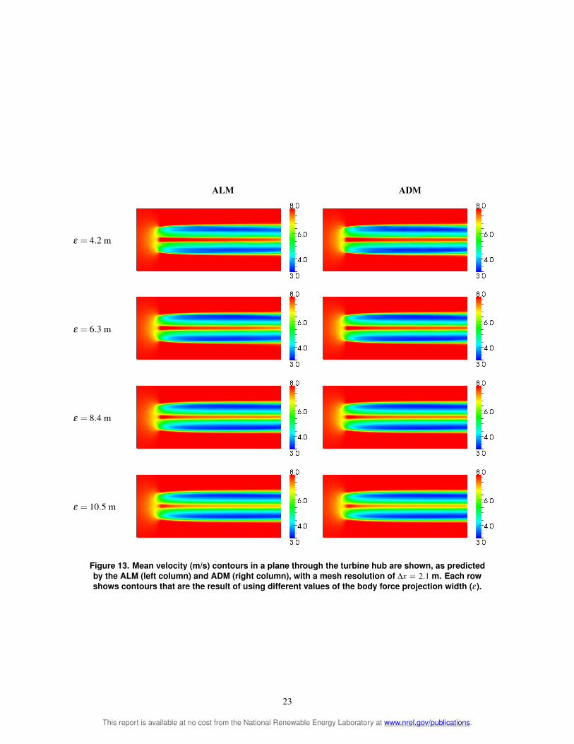
ALM ADM
ε = 42 m
ε = 63 m
ε = 84 m
ε = 105 m
Figure 14 Vorticity magnitude (1s) contours in a plane through the turbine hub are shown as preshydicted by the ALM (left column) and ADM (right column) with a mesh resolution of Δx = 21 m Each
row shows contours that are the result of using different values of the body force projection width (ε)
24
This report is available at no cost from the National Renewable Energy Laboratory at wwwnrelgovpublications
ALM ADM
ε = 42 m
ε = 63 m
ε = 84 m
ε = 105 m
Figure 15 Mean velocity (ms) contours in a plane through the turbine hub are shown as predicted by the ALM (left column) and ADM (right column) with a mesh resolution of Δx = 105 m Each row shows contours that are the result of using different values of the body force projection width (ε)
25
This report is available at no cost from the National Renewable Energy Laboratory at wwwnrelgovpublications
ALM ADM
ε = 42 m
ε = 63 m
ε = 84 m
ε = 105 m
Figure 16 Vorticity magnitude (1s) contours in a plane through the turbine hub are shown as preshydicted by the ALM (left column) and ADM (right column) with a mesh resolution of Δx = 105 m Each row shows contours that are the result of using different values of the body force projection width (ε)
26
This report is available at no cost from the National Renewable Energy Laboratory at wwwnrelgovpublications
Figure 17 Power output for the ALM as a function of actuator point resshyolution along the blade with ε = 84 and a grid resolution of 21 m
Figure 18 Power output as a function of grid resolution for ε = 84 m with and without a tip- and root-loss correction for the ALM
contrast has more points than the ALM and the forces on these points must be calculated for every time-step These differences do not impact the simulation time significantly However time-step size will have a significant impact on simulation time The time-step for simulations performed using the ALM is restricted by the tip speed The tip
27
This report is available at no cost from the National Renewable Energy Laboratory at wwwnrelgovpublications
Figure 19 Power output as a function of time-step for ε = 84 m
of the blade should not pass through more than a single finite-volume cell each time-step This condition is far more restrictive than the typical CFL condition For a case with λ =8 the time-step needs to be eight times smaller using this restriction than with the CFL condition Resolving the root- and tip-vortices compromises the simulation time-step and thus increases computational cost The ADM will provide an accurate solution with a time-step that is based on a CFL condition rather than on tip speed If the simulations require solving the flow structures near the rotor the ALM should be used For simulations related to the far wake the ADM will provide a reasonable solution without compromising the simulation time-step
38 The ε Parameter
A Gaussian function is introduced to turn the set of unphysical point forces into a continuous volume force field The use of a Gaussian function avoids numerical instabilities caused by the application of forces on discrete sections of the blade The width of the function is determined by the ε parameter This parameter plays an important role in the models studied We found that a parameter closest to the characteristic length of the blade section under study yielded the best results The value of the Gaussian function decays to 1 of its initial value at a distance of r = 215ε To span the force of a blade section through the area that covers the distance from the leading edge to the trailing edge a value of ε = c43 would be required With a chord value around 4 m for the NREL 5-MW turbine a value of ε = 4 m43 = 093 m creates numerical instabilities on the grids used in this study Our projections show that making the grid smaller would be expensive unless a fine grid local to the rotor was used
The simulations presented show that as ε becomes smaller the power decreases Note that a small value of ε relashytive to the grid size produces numerical instabilities in the solver These instabilities affect the solution and can be observed in the wake profiles and angle of attack for a case in which ε = 42 m and a grid resolution of 42 m When parameter ε was the same size as the grid size (εΔx = 1) the simulations for the ALM and ADM became unstable This can be avoided by choosing a value of εΔx gt 2 as suggested by Troldborg [9] There is an optimum point for the Gaussian width to match what the BEM theory predicts This optimum is related to the geometry of the blade In this case the solution given by the BEM theory lies somewhere between ε =42 and 21 m It is unclear which value of ε matches the geometry of the blade section and would accurately predict power using the ALM The results
28
This report is available at no cost from the National Renewable Energy Laboratory at wwwnrelgovpublications
Vorticity Mean Velocity
Δt = 0015s
Δt = 003s
Δt = 006s
Δt = 01s
Figure 20 Mean velocity (ms) and vorticity magnitude (1s) contours in a plane through the turbine hub for ε = 84 m are shown Each row shows contours that are the result of using different time-step values
29
This report is available at no cost from the National Renewable Energy Laboratory at wwwnrelgovpublications
suggest that the value of ε should not be fixed to a value that satisfies the condition that ε = c43 A condition that better approximates the physical force distribution of an airfoil should be used varying ε along the span as the chord varies
Increasing the value of ε thickens the shear layer surrounding the wake As the shear layer is thickened there is less vorticity in the flow This is illustrated in Figures 12 14 and 16 as the vorticity decreases with larger ε
30
This report is available at no cost from the National Renewable Energy Laboratory at wwwnrelgovpublications
4 Wind Tunnel Simulations
We have performed a validation of the actuator line model (ALM) that compares the numerical results with the experiments done at the low-speed closed-return wind tunnel at the Department of Energy and Process Engineering at the Norwegian University of Science and Technology Trondheim [26][27] The tunnel has a test section of 185 meters (m) (height) times 271 m (width) times 1115 m (length) The test section height is adjustable to account for wall boundary layer growth In this study we aimed to numerically simulate the experimental setup
We performed simulations for tip speed ratios (λ ) of 3 4 6 9 and 12 and compared the power and thrust coefshyficients against the experimental data In addition we used wake visualizations to illustrate the difference in the breakdown of the wake for different tip speed ratios as well as sampled wake profiles
41 Turbine Model
The turbine modeled has a rotor with a diameter of 0894 m and a tower with a height of 0817 m The blades use the National Renewable Energy Laboratory (NREL) S826 airfoil along the entire span We obtained two-dimensional lift and drag coefficients from the NREL S826 report [28] and corrected for stall delay using NRELrsquos AirfoilPrep tool [29] The actuator line model accounts for only the blades of the turbine and does not include the hub tower or nacelle The turbine is located 366 m from the tunnel inlet and is laterally centered
42 Mesh
The mesh of the tunnel consists of a block with dimensions (1115 m times 1851 m times 271 m) The walls are refined in an attempt to capture the boundary layer The height of the tunnel varies linearly along the streamwise direction from 1801 m to 1851 m The mesh is refined near the walls to capture the boundary layer The walls have a no-slip condition The grid resolution near the wall does not resolve the boundary layer completely but because the rotor is far from the walls we believe the effect of not resolving this boundary layer is negligible The mesh is locally refined near the rotor with ΔxD = 0006 This refinement allows the simulation to calculate power production accurately (following the results from the previous section)
The boundary layer is measured to be 01 m at the tunnel inlet The inlet bulk velocity is taken to be 10 meters per second (ms) The inlet boundary condition is set to match the turbulent boundary layer profile using y 17
U = (41)δ
At y gt δ the velocity is set to 10 ms with no turbulence
43 Results
Power and thrust coefficients are shown as a function of tip speed ratio in Figure 21 The maximum power coeffishycient of 047 is at a tip speed ratio of 6 This corresponds to the highest induction factor as we expected For the case with lowest tip speed ratio the simulation power coefficient lies on top of the experimental data Thrust coefficient is under-predicted for all tip speed ratios
Figure 22 shows wake profiles in the spanwise direction for 1 2 3 and 4 diameters behind the rotor The profiles show how the wake deficit is stronger for higher tip speed ratios Note that for stronger wake deficits the velocity near the edges and in the center of the rotor is larger because of mass conservation Figure 23 shows wake profiles for cases with tip speed ratios of 3 and 6 that are one diameter behind the rotor The wakes in the simulation are different from the experimental data at the center This difference is because the nacelle is not a part of the model It is clear that the nacelle needs to be incorporated into the model to obtain accurate wake profiles As a result this
31
This report is available at no cost from the National Renewable Energy Laboratory at wwwnrelgovpublications
difference causes the thrust to be lower than expected because the nacelle will contribute a drag force to the model For this reason the thrust coefficient curve for the simulations lies below the experimental data Away from the center the wake profiles agree with the experimental data
Figure 24 shows a rendering of the Q-criterion [30] for tip speed ratios of λ = 3 6 9 and 12 The Q-criterion is the second invariant of the velocity gradient tensor Where it is positive it shows regions of the flow where rotation dominates strain and where it is negative strain dominates rotation This illustrates that the breakdown of the wake is faster with increased tip speed ratio With higher tip speed ratio the wake deficit is greater as shown in Figure 22 indicating there is a stronger more unstable wake-edge shear layer This causes faster transition to turbulence and faster wake breakdown The visualizations show that at higher tip speeds the wake starts interacting with the tunnel walls This interaction affects the wake as it is not able to fully expand
The ALM is a good representation of the turbine in the tunnel but is missing some key elements in its implementashytion The model is able to capture the blades inside the flow field Because the power of the turbine is being extracted by the blades the power coefficient is close to what experiments predict However the effect of the nacelle is not included in the model The nacelle contributes to the thrust experienced by the turbine and for this reason the thrust coefficient is under-predicted by the model Tip speed ratio affects the power produced by the turbine and the strucshyture of the wake The maximum power coefficient is reached at a tip speed ratio of 6 which approximates the Betz limit A faster tip speed ratio causes a faster breakdown of the wake
Power Thrust
Figure 21 Power and thrust coefficients as a function of tip speed ratio
32
This report is available at no cost from the National Renewable Energy Laboratory at wwwnrelgovpublications
xD = 1 xD = 2
xD = 3 xD = 4
Figure 22 Mean velocity profiles behind the rotor
33
This report is available at no cost from the National Renewable Energy Laboratory at wwwnrelgovpublications
1D TSR=3 1D TSR=6
3D TSR=3 3D TSR=6
Figure 23 Mean velocity profiles one and three diameters behind the rotor
34
This report is available at no cost from the National Renewable Energy Laboratory at wwwnrelgovpublications
λ = 3 λ = 6
λ = 9 λ = 12
Figure 24 Q-criterion (1s2) rendering showing the structure of the wake for different tip speed ratios
35
This report is available at no cost from the National Renewable Energy Laboratory at wwwnrelgovpublications
5 Wind Farm Simulation
51 Introduction
This section presents the results of a large-eddy simulation (LES) of the flow of over 48 multi-megawatt turbines that compose the Lillgrund wind plant We compared the performance of the actuator line (ALM) and actuator disk model (ADM) in wind farm simulations Churchfield et al [31] performed an LES of the Lillgrund wind farm using the ALM we performed the same simulation using the ADM and compared the results for both models The simulated wind farm is the Lillgrund offshore facility operated by Vattenfall Vindkraft AB Lillgrund is located 7 kilometers (km) off the coast of Sweden and 7 km south of the Oumlresund bridge Figure 25 shows the turbine siting and the computational domain Positive x and y correspond to east and north respectively
We used LES to simulate the atmospheric boundary layer (ABL) with the standard Smagorinsky model We modeled the sea surface as a rough flat surface with an aerodynamic roughness height of 01 millimiters (mm) which was appropriate for the sea surface The turbine model operating at the Lillgrund facility is the Siemens SWT-23-93 The turbine model was provided by Churchfield who reverse-engineered the available turbine information [32] We performed the simulation in two steps running an ABL precursor simulation and running the wind plant simulation The first precursor simulation tried to match the Lillgrund wind conditions as closely as possible and was obtained from Churchfield [31] We chose a mean velocity of 9 ms at hub-height with a wind direction of 2216o At these conditions the turbines operating in Region 2 wake deficits are the strongest We used the turbulent intensity at hub-height of 62 which is typical at the chosen wind direction The precursor simulation was used to create a turbulent wind inlet (west and south) boundary condition on velocity and temperature for the simulation The east and north planes were set to zero gradient for velocity and temperature The velocity top boundary condition was set to zero in the normal direction and to zero gradient in the other two directions The pressure boundary conditions were set to hydrostatic gradient on the top and bottom and to zero gradient on the sides The temperature gradient on the top was set to 0003 Kelvins per meter (Km) to follow the temperature profile in capping inversion The precursor simulation was the same for both the ADM and ALM simulation The time-step of the ALM simulation was fixed at the condition that the tip of the blade should not go through more than one grid cell at each time-step The time-step in the ADM simulation was based on the maximum Courant number not exceeding a limit of 075 The wind plant simulation was for 10 minutes of real time and an initial transient of 150 s
52 Results
Normalized power output is shown for all the rows in the turbine array in Figure 26 Rows B through D are comshypared against field data that were averaged over a year and binned by wind direction Power output for these rows is normalized using the average power of the first turbine in rows B C and D The other turbines are normalized using the power of the first turbine in their row The simulations agree with field data The largest difference is on the last turbines in the rows where the simulation predicted an increase in power production Figure 27 shows non-normalized power output for all the turbines Power production for the ADM agrees well with that for ALM although we observe slight differences The percent difference between the ADM and ALM dimensional power flucshytuated between 1 and 17 Contrasting what we observed in Chapter 3 the ALM produces a slightly higher power output than the ADM The power curve for the model predicts 1347 megawatts (MW) at 9 ms The first turbine in each row is close to this value for both the ADM and ALM although we observed that the ALM usually over predicts power whereas the ADM under predicts power
Figure 28 shows the mean velocity profiles for the ADM and ALM The wake deficits in the ADM simulation are stronger (shown in dark blue) than the ALM Figure 29 shows the difference between the ADM and ALM simulashytions which was calculated by subtracting the ADM data from the ALM data The figure reveals that the regions near the center of the wake have the strongest difference (shown in red)
Figure 30 shows wake profiles along rows C and E The profiles pass through the hub and outboard of the hub in increments of D8 where D is the rotor diameter This shows the wake differences between the models at several
36
This report is available at no cost from the National Renewable Energy Laboratory at wwwnrelgovpublications
Figure 25 Wind farm layout (left) and computational doshymain (right) Illustration by Matthew J Churchfield NREL
locations The biggest difference in wake profiles is on the wake of the first turbine in each row The ADM creates a larger velocity deficit in the center when passing through the first turbine The flow begins to recover in the far wake before hitting the next turbines The ALM and ADM recover to nearly the same value This pattern repeats until the last turbine in the row There is a gap in row E where the flow recovers more than the rest of the turbines This recovery produces more power on the next turbine in the row although the flow is not fully recovered A power production difference of 30 was observed between the turbine right after the gap and the subsequent one The wake recovery in the gap allows greater power production from the next turbine in the row Field data always show a slight increase in power of the third turbine over the second turbine in the row The ALM does not predict this but the ADM does
Figures 32 33 and 34 show wake profiles for turbines 27 through 30 and at 05 075 and 1 diameter behind the rotor The profiles show that the velocity deficit near the center of the wake for the ADM is stronger than that of the ALM However moving towards the edge of the wake the velocity deficit from the ALM is stronger than for the ADM
The time-step used for the ALM simulation was Δt =0015 s while the time-step for the ADM simulation was based on a Courant-Friedrichs-Lewy number of 075 with typical values close to Δt =006 s The difference in time-step may cause the power output differences that were observed Figure 19 shows that as Δt increases predicted power decreases similar to what Figure 27 shows
The ADM simulation was completed two times faster than the ALM simulation The ALM simulation required about 1 million CPU-hours whereas the ADM showed significant savings This difference is because the ADM has a higher time-step On a time per time-step basis the ADM takes longer to calculate all the body forces on the disk (rather than just the body forces on the blades of the ALM)
The ALM and ADM provide similar results in large-scale wind farm simulations There is a difference in power production in which the ALM produces more power than the ADM The difference in the first row of turbines is larger than the turbines that are further downstream In terms of computational cost the ADM can be run faster because time-step is not limited to tip speed The ADM simulation was completed three times faster than the ALM This time reduction is crucial when performing these type of simulations The wake in the ADM has a greater deficit
37
This report is available at no cost from the National Renewable Energy Laboratory at wwwnrelgovpublications
in the center than the ALM However the velocity deficit near the edges is stronger for the ALM indicating a larger power extraction is near the outer portion of the blades The total difference shows that the power extraction for the ALM is greater than that for the ADM
38
This report is available at no cost from the National Renewable Energy Laboratory at wwwnrelgovpublications
Row A Row B
Row C Row D
Row E Row F
Row G Row H
macrFigure 26 Ten minute average power produced by each turbine Pi normalized by the power of the first turbine in the row Average over one year of field data is shown for rows B-D
39
This report is available at no cost from the National Renewable Energy Laboratory at wwwnrelgovpublications
Row A Row B
Row C Row D
Row E Row F
Row G Row H
Figure 27 Power produced by each turbine
40
This report is available at no cost from the National Renewable Energy Laboratory at wwwnrelgovpublications
ADM ALM
Figure 28 Mean velocity (ms) contours at hub height for ADM (left) and ALM (right)
Figure 29 Mean velocity difference (ms) between ALM and ADM (ALM-ADM)
41
This report is available at no cost from the National Renewable Energy Laboratory at wwwnrelgovpublications
Row C Row E
yR = 0
yR = 025
yR = 05
yR = 075
yR = 1
Figure 30 Mean streamwise velocity profiles at hub height along rows C and E at various horizontal locations outboard of hub ranging from hub to blade tip
Turbine 30 Turbine 29
Turbine 28 Turbine 27
Figure 31 Mean velocity in the cross stream direction at one-fourth diameter behind the rotor for turbines in row D
42
This report is available at no cost from the National Renewable Energy Laboratory at wwwnrelgovpublications
Turbine 30 Turbine 29
Turbine 28 Turbine 27
Figure 32 Mean velocity in the cross stream direction at one-half diameter behind the rotor for turbines in row D
Turbine 30 Turbine 29
Turbine 28 Turbine 27
Figure 33 Mean velocity in the cross stream direction at three-fourths diameter behind the rotor for turbines in row D
43
This report is available at no cost from the National Renewable Energy Laboratory at wwwnrelgovpublications
Turbine 30 Turbine 29
Turbine 28 Turbine 27
Figure 34 Mean velocity in the cross stream direction at 1 diameter behind the rotor for turbines in row D
Turbine 30 Turbine 29
Turbine 28 Turbine 27
Figure 35 Mean velocity in the cross stream direction at 3 diameters behind the rotor for turbines in row D
44
This report is available at no cost from the National Renewable Energy Laboratory at wwwnrelgovpublications
Turbine 30 Turbine 29
Turbine 28 Turbine 27
Figure 36 Mean velocity in the cross stream direction at 4 diameters behind the rotor for turbines in row D
45
This report is available at no cost from the National Renewable Energy Laboratory at wwwnrelgovpublications
6 Conclusion and Future Work
The actuator line model (ALM) and actuator disk model (ADM) are a suitable representation of a wind turbine when using numerical simulations of fluid flows The models do not require that the full geometry of the blades be resolved and in which case model them as a set of points in the flow The ALM models the blades as a set of points along each blade axis whereas the ADM models the rotor as a disk with points that represent sections of the disk
The ADM and ALM provide very similar results in simulations with uniform inflow There is a clear grid depenshydence on power production and wake profiles of the ADM and ALM As the grid is refined the predicted power increases for both models Using a Glauert tip-loss correction with the ALM decreases the power production The number of actuator points in the ALM should be adequate to account for all the sections of the blade and provide smooth changes between them We recommend using a value smaller than ΔbΔx = 075 Mean wake profiles are similar for both the ADM and ALM
A Gaussian function was introduced to avoid numerical instabilities that are caused by the application of forces on discrete sections of the blade The width of the function was determined by the ε parameter This parameter played an important role in the models studied We observed that a parameter closest to the characteristic length of the blade section yielded the best results As the width of the projection function is decreased both the ALM and ADM predicted power decreases but never converges upon a value A specific value of epsilon allows agreement with blade-element momentum theory predictions However the ε parameter must be higher than 2Δx to avoid numerical instabilities in the solver
The ALM resolves the flow structures that are caused by the presence of individual blades which the ADM does not The ALM matches the physics more closely because it captures the root- and tip-vortices which the ADM does not Also the ALM is able to capture helical and asymmetric structures across the wake which caused asymmetric roll-up of Kelvin-Helmholtz-like instabilities in the wakersquos outer shear layer The ALM captures the vortical structures in the near wake ADM provides good results in the far wake but does not produce the vortical structures near the rotor If simulations are intended to determine the far wake effects the ADM should provide reasonable results
We used the ALM to validate a small-scale wind tunnel experiment and compared the structure of the wake for different tip speed ratios We observed that as the tip speed ratio is higher the breakdown of the wake occurs faster leaving a wider wake for larger tip speed ratios The tunnel walls play an important role in the simulation as the wake interacts with the walls The blockage effect of the turbine makes the reference velocity of the tunnel higher near the rotor than on the inlet
When performing large-scale wind farm simulations we found that the models perform well ALM produces slightly more power than ADM under atmospheric boundary layer conditions It is still unknown why this occurs but it is possible that the difference is caused by the time-step difference in the simulations The wake of the ADM is different from that of the ALM The ADM wake has a stronger wake deficit near the center whereas the ALM has a stronger wake deficit near the edges Wake profiles are similar but we observed that the greatest difference in the near wake primarily in the first row of turbines
46
This report is available at no cost from the National Renewable Energy Laboratory at wwwnrelgovpublications
Bibliography
[1] JN Soslashrensen Aerodynamics aspects of wind energy conversion 43427ndash448 September 2010
[2] T Burton D Sharpe N Jenkins and E Bossanyi Aerodynamics of Horizontal-Axis Wind Turbines pages 41ndash172 John Wiley amp Sons Ltd 2002
[3] JF Manwell JG McGowan and AL Rogers Wind Energy Explained Theory Design and Application Wiley 2010
[4] B Sanderse SP van der Pijl and B Koren Review of computational fluid dynamics for wind turbine wake aerodynamics Wind Energy 14 2011
[5] F Porteacute-Agel H Lu and YT Wu A Large-Eddy simulation framework for wind energy applications The Fifth International Symposium on Computational Wind Engineering (CWE2010) Chapel Hill North Carolina USA May 23-27 2010
[6] M Calaf C Meneveau and J Meyers Large eddy simulation study of fully developed wind-turbine array boundary layers Physics of Fluids 22(1)015110 2010
[7] N Troldborg JN Soslashrensen and R Mikkelsen Numerical simulations of wake charasteristics of a wind turbine in uniform flow 1386ndash99 2009
[8] T Phuoc Aeacuterodynamique instationnaire turbulente - aspects numeacuteriques et expeacuterimentaux Journeacute theacutematique DRET 1994
[9] N Troldborg Actuator Line Modeling of Wind Turbine Wakes PhD thesis Technical University of Denmark Lyngby Denmark 2008
[10] I Ammara C Leclerc and C Masson A viscous three-dimensional differentialactuator-disk method for the aerodynamic analysis of wind farms Journal of Solar Energy Engineering 124(4)345ndash356 2002
[11] A Jimenez A Crespo E Migoya and J Garcia Advances in large-eddy simulation of a wind turbine wake Journal of Physics Conference Series 75(1)012041 2007
[12] C Masson A Smaiumlli and C Leclerc Aerodynamic analysis of hawts operating in unsteady conditions Wind Energy 4(1)1ndash22 2001
[13] R Mikkelsen JN Soslashrensen and WZ Shen Modelling and analysis of the flow field around a coned rotor Wind Energy 4(3)121ndash135 2001
[14] JN Soslashrensen and WZ Shen Numerical modeling of wind turbine wakes Journal of Fluids Engineering 124(2)393ndash399 June 2002
[15] SSA Ivanell JN Soslashrensen R Mikkelsen and D Henningson Analysis of numerically generated wake structures Wind Energy 12(1)63ndash80 2009
[16] R Mikkelsen JN Soslashrensen S Oslashye and N Troldborg Analysis of power enhancement for a row of wind turbines using the actuator line technique Journal of Physics Conference Series ndash The Science of Making Torque from Wind 75(012044) 2007
[17] R Mikkelsen Actuator Disc Methods Applied to Wind Turbines PhD thesis Technical University of Denmark Mechanical Engineering Department 2003
[18] WZ Shen JH Zhang and JN Soslashrensen The actuator surface model A new navierndashstokes based model for rotor computations Journal of Solar Energy Engineering 131(1)011002 2009
47
This report is available at no cost from the National Renewable Energy Laboratory at wwwnrelgovpublications
[19] I Dobrev F Massouh and M Rapin Actuator surface hybrid model Journal of Physics Conference Series 75(1)012019 2007
[20] CS Watters and C Masson Modeling of lifting-device aerodynamics using the actuator surface concept International Journal for Numerical Methods in Fluids 62(11)1264ndash1298 2010
[21] OpenFOAM Ver 171 [available online] Silicon Graphics International Corporation (SGI) URL httpwwwopenfoamorgarchive171download [accessed 13 December 2011]
[22] J Smagorinsky General circulation experiments with the primitive equations Monthly Weather Review 9199ndash164 1963
[23] MJ Buhl WT_Perf Userrsquos Guide National Renewable Energy Laboratory 2004
[24] H Glauert Airplane Propellers pages 251ndash268 Dover New York 1985
[25] J Jonkman S Butterfield W Musial and G Scott Definition of a 5-MW reference wind turbine for offshore system development Technical Report NRELTP-500-38060
[26] MS Adaramola and P-A Krogstad Experimental investigation of wake effects on wind turbine performance Renewable Energy 362078ndash2086 2011
[27] P-A Krogstad and JA Lund An experimental and numerical study of the performance of a model turbine Wind Energy 2011
[28] DM Somers The S825 and S826 Airfoils Period of Performance 1994ndash1995 The S825 and S826 Airfoils Technical Report January 2005
[29] NWTC Design Codes (AirfoilPrep by Dr Craig Hansen) httpwindnrelgovdesigncodespreprocessorsairfoilprep [Accessed 21 February 2012]
[30] JCR Hunt AA Wray and P Moin Eddies streams and convergence zones in turbulent flows (1970) 1988
[31] MJ Churchfield S Lee P Moriarty LA Martiacutenez S Leonardi G Vijayakumar and JG Brasseur A large-eddy simulation of wind-plant aerodynamics 50th AIAA Aerospace Sciences Meeting Nashville Tennessee USA 2012
[32] MJ Churchield A Method for Designing Generic Wind Turbine Models Representative of Real Turbines and Generic Siemens SWT-23-93 and Vestas V80 Specifications National Renewable Energy Laboratory 2012
48
This report is available at no cost from the National Renewable Energy Laboratory at wwwnrelgovpublications
- Literature Review
-
- Introduction
- Basics of Wind Turbine Aerodynamics
- Wind Turbine Computational Fluid Dynamics
- Atmospheric Boundary Layer Simulations
- Actuator Disc Model (ADM)
- Actuator Line Model (ALM)
- Actuator Surface Model (ASM)
- Comparison Between ADM and ALM
- Conclusions
-
- Actuator Turbine Model Implementation
-
- Actuator Line Model
- Actuator Disk Model
- Numerical Method
-
- Actuator Disk and Actuator Line Models in Uniform Nonturbulent Inflow
-
- Five Megawatt Reference Turbine
- Actuator Line Model
- Actuator Disk Model
- Actuator Points
- Tip Loss Correction
- Time-step
- Comparison
- The Parameter
-
- Wind Tunnel Simulations
-
- Turbine Model
- Mesh
- Results
-
- Wind Farm Simulation
-
- Introduction
- Results
-
- Conclusion and Future Work
- Bibliography
-
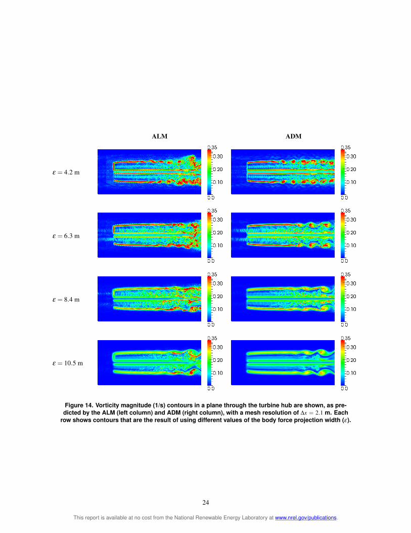
ALM ADM
ε = 42 m
ε = 63 m
ε = 84 m
ε = 105 m
Figure 16 Vorticity magnitude (1s) contours in a plane through the turbine hub are shown as preshydicted by the ALM (left column) and ADM (right column) with a mesh resolution of Δx = 105 m Each row shows contours that are the result of using different values of the body force projection width (ε)
26
This report is available at no cost from the National Renewable Energy Laboratory at wwwnrelgovpublications
Figure 17 Power output for the ALM as a function of actuator point resshyolution along the blade with ε = 84 and a grid resolution of 21 m
Figure 18 Power output as a function of grid resolution for ε = 84 m with and without a tip- and root-loss correction for the ALM
contrast has more points than the ALM and the forces on these points must be calculated for every time-step These differences do not impact the simulation time significantly However time-step size will have a significant impact on simulation time The time-step for simulations performed using the ALM is restricted by the tip speed The tip
27
This report is available at no cost from the National Renewable Energy Laboratory at wwwnrelgovpublications
Figure 19 Power output as a function of time-step for ε = 84 m
of the blade should not pass through more than a single finite-volume cell each time-step This condition is far more restrictive than the typical CFL condition For a case with λ =8 the time-step needs to be eight times smaller using this restriction than with the CFL condition Resolving the root- and tip-vortices compromises the simulation time-step and thus increases computational cost The ADM will provide an accurate solution with a time-step that is based on a CFL condition rather than on tip speed If the simulations require solving the flow structures near the rotor the ALM should be used For simulations related to the far wake the ADM will provide a reasonable solution without compromising the simulation time-step
38 The ε Parameter
A Gaussian function is introduced to turn the set of unphysical point forces into a continuous volume force field The use of a Gaussian function avoids numerical instabilities caused by the application of forces on discrete sections of the blade The width of the function is determined by the ε parameter This parameter plays an important role in the models studied We found that a parameter closest to the characteristic length of the blade section under study yielded the best results The value of the Gaussian function decays to 1 of its initial value at a distance of r = 215ε To span the force of a blade section through the area that covers the distance from the leading edge to the trailing edge a value of ε = c43 would be required With a chord value around 4 m for the NREL 5-MW turbine a value of ε = 4 m43 = 093 m creates numerical instabilities on the grids used in this study Our projections show that making the grid smaller would be expensive unless a fine grid local to the rotor was used
The simulations presented show that as ε becomes smaller the power decreases Note that a small value of ε relashytive to the grid size produces numerical instabilities in the solver These instabilities affect the solution and can be observed in the wake profiles and angle of attack for a case in which ε = 42 m and a grid resolution of 42 m When parameter ε was the same size as the grid size (εΔx = 1) the simulations for the ALM and ADM became unstable This can be avoided by choosing a value of εΔx gt 2 as suggested by Troldborg [9] There is an optimum point for the Gaussian width to match what the BEM theory predicts This optimum is related to the geometry of the blade In this case the solution given by the BEM theory lies somewhere between ε =42 and 21 m It is unclear which value of ε matches the geometry of the blade section and would accurately predict power using the ALM The results
28
This report is available at no cost from the National Renewable Energy Laboratory at wwwnrelgovpublications
Vorticity Mean Velocity
Δt = 0015s
Δt = 003s
Δt = 006s
Δt = 01s
Figure 20 Mean velocity (ms) and vorticity magnitude (1s) contours in a plane through the turbine hub for ε = 84 m are shown Each row shows contours that are the result of using different time-step values
29
This report is available at no cost from the National Renewable Energy Laboratory at wwwnrelgovpublications
suggest that the value of ε should not be fixed to a value that satisfies the condition that ε = c43 A condition that better approximates the physical force distribution of an airfoil should be used varying ε along the span as the chord varies
Increasing the value of ε thickens the shear layer surrounding the wake As the shear layer is thickened there is less vorticity in the flow This is illustrated in Figures 12 14 and 16 as the vorticity decreases with larger ε
30
This report is available at no cost from the National Renewable Energy Laboratory at wwwnrelgovpublications
4 Wind Tunnel Simulations
We have performed a validation of the actuator line model (ALM) that compares the numerical results with the experiments done at the low-speed closed-return wind tunnel at the Department of Energy and Process Engineering at the Norwegian University of Science and Technology Trondheim [26][27] The tunnel has a test section of 185 meters (m) (height) times 271 m (width) times 1115 m (length) The test section height is adjustable to account for wall boundary layer growth In this study we aimed to numerically simulate the experimental setup
We performed simulations for tip speed ratios (λ ) of 3 4 6 9 and 12 and compared the power and thrust coefshyficients against the experimental data In addition we used wake visualizations to illustrate the difference in the breakdown of the wake for different tip speed ratios as well as sampled wake profiles
41 Turbine Model
The turbine modeled has a rotor with a diameter of 0894 m and a tower with a height of 0817 m The blades use the National Renewable Energy Laboratory (NREL) S826 airfoil along the entire span We obtained two-dimensional lift and drag coefficients from the NREL S826 report [28] and corrected for stall delay using NRELrsquos AirfoilPrep tool [29] The actuator line model accounts for only the blades of the turbine and does not include the hub tower or nacelle The turbine is located 366 m from the tunnel inlet and is laterally centered
42 Mesh
The mesh of the tunnel consists of a block with dimensions (1115 m times 1851 m times 271 m) The walls are refined in an attempt to capture the boundary layer The height of the tunnel varies linearly along the streamwise direction from 1801 m to 1851 m The mesh is refined near the walls to capture the boundary layer The walls have a no-slip condition The grid resolution near the wall does not resolve the boundary layer completely but because the rotor is far from the walls we believe the effect of not resolving this boundary layer is negligible The mesh is locally refined near the rotor with ΔxD = 0006 This refinement allows the simulation to calculate power production accurately (following the results from the previous section)
The boundary layer is measured to be 01 m at the tunnel inlet The inlet bulk velocity is taken to be 10 meters per second (ms) The inlet boundary condition is set to match the turbulent boundary layer profile using y 17
U = (41)δ
At y gt δ the velocity is set to 10 ms with no turbulence
43 Results
Power and thrust coefficients are shown as a function of tip speed ratio in Figure 21 The maximum power coeffishycient of 047 is at a tip speed ratio of 6 This corresponds to the highest induction factor as we expected For the case with lowest tip speed ratio the simulation power coefficient lies on top of the experimental data Thrust coefficient is under-predicted for all tip speed ratios
Figure 22 shows wake profiles in the spanwise direction for 1 2 3 and 4 diameters behind the rotor The profiles show how the wake deficit is stronger for higher tip speed ratios Note that for stronger wake deficits the velocity near the edges and in the center of the rotor is larger because of mass conservation Figure 23 shows wake profiles for cases with tip speed ratios of 3 and 6 that are one diameter behind the rotor The wakes in the simulation are different from the experimental data at the center This difference is because the nacelle is not a part of the model It is clear that the nacelle needs to be incorporated into the model to obtain accurate wake profiles As a result this
31
This report is available at no cost from the National Renewable Energy Laboratory at wwwnrelgovpublications
difference causes the thrust to be lower than expected because the nacelle will contribute a drag force to the model For this reason the thrust coefficient curve for the simulations lies below the experimental data Away from the center the wake profiles agree with the experimental data
Figure 24 shows a rendering of the Q-criterion [30] for tip speed ratios of λ = 3 6 9 and 12 The Q-criterion is the second invariant of the velocity gradient tensor Where it is positive it shows regions of the flow where rotation dominates strain and where it is negative strain dominates rotation This illustrates that the breakdown of the wake is faster with increased tip speed ratio With higher tip speed ratio the wake deficit is greater as shown in Figure 22 indicating there is a stronger more unstable wake-edge shear layer This causes faster transition to turbulence and faster wake breakdown The visualizations show that at higher tip speeds the wake starts interacting with the tunnel walls This interaction affects the wake as it is not able to fully expand
The ALM is a good representation of the turbine in the tunnel but is missing some key elements in its implementashytion The model is able to capture the blades inside the flow field Because the power of the turbine is being extracted by the blades the power coefficient is close to what experiments predict However the effect of the nacelle is not included in the model The nacelle contributes to the thrust experienced by the turbine and for this reason the thrust coefficient is under-predicted by the model Tip speed ratio affects the power produced by the turbine and the strucshyture of the wake The maximum power coefficient is reached at a tip speed ratio of 6 which approximates the Betz limit A faster tip speed ratio causes a faster breakdown of the wake
Power Thrust
Figure 21 Power and thrust coefficients as a function of tip speed ratio
32
This report is available at no cost from the National Renewable Energy Laboratory at wwwnrelgovpublications
xD = 1 xD = 2
xD = 3 xD = 4
Figure 22 Mean velocity profiles behind the rotor
33
This report is available at no cost from the National Renewable Energy Laboratory at wwwnrelgovpublications
1D TSR=3 1D TSR=6
3D TSR=3 3D TSR=6
Figure 23 Mean velocity profiles one and three diameters behind the rotor
34
This report is available at no cost from the National Renewable Energy Laboratory at wwwnrelgovpublications
λ = 3 λ = 6
λ = 9 λ = 12
Figure 24 Q-criterion (1s2) rendering showing the structure of the wake for different tip speed ratios
35
This report is available at no cost from the National Renewable Energy Laboratory at wwwnrelgovpublications
5 Wind Farm Simulation
51 Introduction
This section presents the results of a large-eddy simulation (LES) of the flow of over 48 multi-megawatt turbines that compose the Lillgrund wind plant We compared the performance of the actuator line (ALM) and actuator disk model (ADM) in wind farm simulations Churchfield et al [31] performed an LES of the Lillgrund wind farm using the ALM we performed the same simulation using the ADM and compared the results for both models The simulated wind farm is the Lillgrund offshore facility operated by Vattenfall Vindkraft AB Lillgrund is located 7 kilometers (km) off the coast of Sweden and 7 km south of the Oumlresund bridge Figure 25 shows the turbine siting and the computational domain Positive x and y correspond to east and north respectively
We used LES to simulate the atmospheric boundary layer (ABL) with the standard Smagorinsky model We modeled the sea surface as a rough flat surface with an aerodynamic roughness height of 01 millimiters (mm) which was appropriate for the sea surface The turbine model operating at the Lillgrund facility is the Siemens SWT-23-93 The turbine model was provided by Churchfield who reverse-engineered the available turbine information [32] We performed the simulation in two steps running an ABL precursor simulation and running the wind plant simulation The first precursor simulation tried to match the Lillgrund wind conditions as closely as possible and was obtained from Churchfield [31] We chose a mean velocity of 9 ms at hub-height with a wind direction of 2216o At these conditions the turbines operating in Region 2 wake deficits are the strongest We used the turbulent intensity at hub-height of 62 which is typical at the chosen wind direction The precursor simulation was used to create a turbulent wind inlet (west and south) boundary condition on velocity and temperature for the simulation The east and north planes were set to zero gradient for velocity and temperature The velocity top boundary condition was set to zero in the normal direction and to zero gradient in the other two directions The pressure boundary conditions were set to hydrostatic gradient on the top and bottom and to zero gradient on the sides The temperature gradient on the top was set to 0003 Kelvins per meter (Km) to follow the temperature profile in capping inversion The precursor simulation was the same for both the ADM and ALM simulation The time-step of the ALM simulation was fixed at the condition that the tip of the blade should not go through more than one grid cell at each time-step The time-step in the ADM simulation was based on the maximum Courant number not exceeding a limit of 075 The wind plant simulation was for 10 minutes of real time and an initial transient of 150 s
52 Results
Normalized power output is shown for all the rows in the turbine array in Figure 26 Rows B through D are comshypared against field data that were averaged over a year and binned by wind direction Power output for these rows is normalized using the average power of the first turbine in rows B C and D The other turbines are normalized using the power of the first turbine in their row The simulations agree with field data The largest difference is on the last turbines in the rows where the simulation predicted an increase in power production Figure 27 shows non-normalized power output for all the turbines Power production for the ADM agrees well with that for ALM although we observe slight differences The percent difference between the ADM and ALM dimensional power flucshytuated between 1 and 17 Contrasting what we observed in Chapter 3 the ALM produces a slightly higher power output than the ADM The power curve for the model predicts 1347 megawatts (MW) at 9 ms The first turbine in each row is close to this value for both the ADM and ALM although we observed that the ALM usually over predicts power whereas the ADM under predicts power
Figure 28 shows the mean velocity profiles for the ADM and ALM The wake deficits in the ADM simulation are stronger (shown in dark blue) than the ALM Figure 29 shows the difference between the ADM and ALM simulashytions which was calculated by subtracting the ADM data from the ALM data The figure reveals that the regions near the center of the wake have the strongest difference (shown in red)
Figure 30 shows wake profiles along rows C and E The profiles pass through the hub and outboard of the hub in increments of D8 where D is the rotor diameter This shows the wake differences between the models at several
36
This report is available at no cost from the National Renewable Energy Laboratory at wwwnrelgovpublications
Figure 25 Wind farm layout (left) and computational doshymain (right) Illustration by Matthew J Churchfield NREL
locations The biggest difference in wake profiles is on the wake of the first turbine in each row The ADM creates a larger velocity deficit in the center when passing through the first turbine The flow begins to recover in the far wake before hitting the next turbines The ALM and ADM recover to nearly the same value This pattern repeats until the last turbine in the row There is a gap in row E where the flow recovers more than the rest of the turbines This recovery produces more power on the next turbine in the row although the flow is not fully recovered A power production difference of 30 was observed between the turbine right after the gap and the subsequent one The wake recovery in the gap allows greater power production from the next turbine in the row Field data always show a slight increase in power of the third turbine over the second turbine in the row The ALM does not predict this but the ADM does
Figures 32 33 and 34 show wake profiles for turbines 27 through 30 and at 05 075 and 1 diameter behind the rotor The profiles show that the velocity deficit near the center of the wake for the ADM is stronger than that of the ALM However moving towards the edge of the wake the velocity deficit from the ALM is stronger than for the ADM
The time-step used for the ALM simulation was Δt =0015 s while the time-step for the ADM simulation was based on a Courant-Friedrichs-Lewy number of 075 with typical values close to Δt =006 s The difference in time-step may cause the power output differences that were observed Figure 19 shows that as Δt increases predicted power decreases similar to what Figure 27 shows
The ADM simulation was completed two times faster than the ALM simulation The ALM simulation required about 1 million CPU-hours whereas the ADM showed significant savings This difference is because the ADM has a higher time-step On a time per time-step basis the ADM takes longer to calculate all the body forces on the disk (rather than just the body forces on the blades of the ALM)
The ALM and ADM provide similar results in large-scale wind farm simulations There is a difference in power production in which the ALM produces more power than the ADM The difference in the first row of turbines is larger than the turbines that are further downstream In terms of computational cost the ADM can be run faster because time-step is not limited to tip speed The ADM simulation was completed three times faster than the ALM This time reduction is crucial when performing these type of simulations The wake in the ADM has a greater deficit
37
This report is available at no cost from the National Renewable Energy Laboratory at wwwnrelgovpublications
in the center than the ALM However the velocity deficit near the edges is stronger for the ALM indicating a larger power extraction is near the outer portion of the blades The total difference shows that the power extraction for the ALM is greater than that for the ADM
38
This report is available at no cost from the National Renewable Energy Laboratory at wwwnrelgovpublications
Row A Row B
Row C Row D
Row E Row F
Row G Row H
macrFigure 26 Ten minute average power produced by each turbine Pi normalized by the power of the first turbine in the row Average over one year of field data is shown for rows B-D
39
This report is available at no cost from the National Renewable Energy Laboratory at wwwnrelgovpublications
Row A Row B
Row C Row D
Row E Row F
Row G Row H
Figure 27 Power produced by each turbine
40
This report is available at no cost from the National Renewable Energy Laboratory at wwwnrelgovpublications
ADM ALM
Figure 28 Mean velocity (ms) contours at hub height for ADM (left) and ALM (right)
Figure 29 Mean velocity difference (ms) between ALM and ADM (ALM-ADM)
41
This report is available at no cost from the National Renewable Energy Laboratory at wwwnrelgovpublications
Row C Row E
yR = 0
yR = 025
yR = 05
yR = 075
yR = 1
Figure 30 Mean streamwise velocity profiles at hub height along rows C and E at various horizontal locations outboard of hub ranging from hub to blade tip
Turbine 30 Turbine 29
Turbine 28 Turbine 27
Figure 31 Mean velocity in the cross stream direction at one-fourth diameter behind the rotor for turbines in row D
42
This report is available at no cost from the National Renewable Energy Laboratory at wwwnrelgovpublications
Turbine 30 Turbine 29
Turbine 28 Turbine 27
Figure 32 Mean velocity in the cross stream direction at one-half diameter behind the rotor for turbines in row D
Turbine 30 Turbine 29
Turbine 28 Turbine 27
Figure 33 Mean velocity in the cross stream direction at three-fourths diameter behind the rotor for turbines in row D
43
This report is available at no cost from the National Renewable Energy Laboratory at wwwnrelgovpublications
Turbine 30 Turbine 29
Turbine 28 Turbine 27
Figure 34 Mean velocity in the cross stream direction at 1 diameter behind the rotor for turbines in row D
Turbine 30 Turbine 29
Turbine 28 Turbine 27
Figure 35 Mean velocity in the cross stream direction at 3 diameters behind the rotor for turbines in row D
44
This report is available at no cost from the National Renewable Energy Laboratory at wwwnrelgovpublications
Turbine 30 Turbine 29
Turbine 28 Turbine 27
Figure 36 Mean velocity in the cross stream direction at 4 diameters behind the rotor for turbines in row D
45
This report is available at no cost from the National Renewable Energy Laboratory at wwwnrelgovpublications
6 Conclusion and Future Work
The actuator line model (ALM) and actuator disk model (ADM) are a suitable representation of a wind turbine when using numerical simulations of fluid flows The models do not require that the full geometry of the blades be resolved and in which case model them as a set of points in the flow The ALM models the blades as a set of points along each blade axis whereas the ADM models the rotor as a disk with points that represent sections of the disk
The ADM and ALM provide very similar results in simulations with uniform inflow There is a clear grid depenshydence on power production and wake profiles of the ADM and ALM As the grid is refined the predicted power increases for both models Using a Glauert tip-loss correction with the ALM decreases the power production The number of actuator points in the ALM should be adequate to account for all the sections of the blade and provide smooth changes between them We recommend using a value smaller than ΔbΔx = 075 Mean wake profiles are similar for both the ADM and ALM
A Gaussian function was introduced to avoid numerical instabilities that are caused by the application of forces on discrete sections of the blade The width of the function was determined by the ε parameter This parameter played an important role in the models studied We observed that a parameter closest to the characteristic length of the blade section yielded the best results As the width of the projection function is decreased both the ALM and ADM predicted power decreases but never converges upon a value A specific value of epsilon allows agreement with blade-element momentum theory predictions However the ε parameter must be higher than 2Δx to avoid numerical instabilities in the solver
The ALM resolves the flow structures that are caused by the presence of individual blades which the ADM does not The ALM matches the physics more closely because it captures the root- and tip-vortices which the ADM does not Also the ALM is able to capture helical and asymmetric structures across the wake which caused asymmetric roll-up of Kelvin-Helmholtz-like instabilities in the wakersquos outer shear layer The ALM captures the vortical structures in the near wake ADM provides good results in the far wake but does not produce the vortical structures near the rotor If simulations are intended to determine the far wake effects the ADM should provide reasonable results
We used the ALM to validate a small-scale wind tunnel experiment and compared the structure of the wake for different tip speed ratios We observed that as the tip speed ratio is higher the breakdown of the wake occurs faster leaving a wider wake for larger tip speed ratios The tunnel walls play an important role in the simulation as the wake interacts with the walls The blockage effect of the turbine makes the reference velocity of the tunnel higher near the rotor than on the inlet
When performing large-scale wind farm simulations we found that the models perform well ALM produces slightly more power than ADM under atmospheric boundary layer conditions It is still unknown why this occurs but it is possible that the difference is caused by the time-step difference in the simulations The wake of the ADM is different from that of the ALM The ADM wake has a stronger wake deficit near the center whereas the ALM has a stronger wake deficit near the edges Wake profiles are similar but we observed that the greatest difference in the near wake primarily in the first row of turbines
46
This report is available at no cost from the National Renewable Energy Laboratory at wwwnrelgovpublications
Bibliography
[1] JN Soslashrensen Aerodynamics aspects of wind energy conversion 43427ndash448 September 2010
[2] T Burton D Sharpe N Jenkins and E Bossanyi Aerodynamics of Horizontal-Axis Wind Turbines pages 41ndash172 John Wiley amp Sons Ltd 2002
[3] JF Manwell JG McGowan and AL Rogers Wind Energy Explained Theory Design and Application Wiley 2010
[4] B Sanderse SP van der Pijl and B Koren Review of computational fluid dynamics for wind turbine wake aerodynamics Wind Energy 14 2011
[5] F Porteacute-Agel H Lu and YT Wu A Large-Eddy simulation framework for wind energy applications The Fifth International Symposium on Computational Wind Engineering (CWE2010) Chapel Hill North Carolina USA May 23-27 2010
[6] M Calaf C Meneveau and J Meyers Large eddy simulation study of fully developed wind-turbine array boundary layers Physics of Fluids 22(1)015110 2010
[7] N Troldborg JN Soslashrensen and R Mikkelsen Numerical simulations of wake charasteristics of a wind turbine in uniform flow 1386ndash99 2009
[8] T Phuoc Aeacuterodynamique instationnaire turbulente - aspects numeacuteriques et expeacuterimentaux Journeacute theacutematique DRET 1994
[9] N Troldborg Actuator Line Modeling of Wind Turbine Wakes PhD thesis Technical University of Denmark Lyngby Denmark 2008
[10] I Ammara C Leclerc and C Masson A viscous three-dimensional differentialactuator-disk method for the aerodynamic analysis of wind farms Journal of Solar Energy Engineering 124(4)345ndash356 2002
[11] A Jimenez A Crespo E Migoya and J Garcia Advances in large-eddy simulation of a wind turbine wake Journal of Physics Conference Series 75(1)012041 2007
[12] C Masson A Smaiumlli and C Leclerc Aerodynamic analysis of hawts operating in unsteady conditions Wind Energy 4(1)1ndash22 2001
[13] R Mikkelsen JN Soslashrensen and WZ Shen Modelling and analysis of the flow field around a coned rotor Wind Energy 4(3)121ndash135 2001
[14] JN Soslashrensen and WZ Shen Numerical modeling of wind turbine wakes Journal of Fluids Engineering 124(2)393ndash399 June 2002
[15] SSA Ivanell JN Soslashrensen R Mikkelsen and D Henningson Analysis of numerically generated wake structures Wind Energy 12(1)63ndash80 2009
[16] R Mikkelsen JN Soslashrensen S Oslashye and N Troldborg Analysis of power enhancement for a row of wind turbines using the actuator line technique Journal of Physics Conference Series ndash The Science of Making Torque from Wind 75(012044) 2007
[17] R Mikkelsen Actuator Disc Methods Applied to Wind Turbines PhD thesis Technical University of Denmark Mechanical Engineering Department 2003
[18] WZ Shen JH Zhang and JN Soslashrensen The actuator surface model A new navierndashstokes based model for rotor computations Journal of Solar Energy Engineering 131(1)011002 2009
47
This report is available at no cost from the National Renewable Energy Laboratory at wwwnrelgovpublications
[19] I Dobrev F Massouh and M Rapin Actuator surface hybrid model Journal of Physics Conference Series 75(1)012019 2007
[20] CS Watters and C Masson Modeling of lifting-device aerodynamics using the actuator surface concept International Journal for Numerical Methods in Fluids 62(11)1264ndash1298 2010
[21] OpenFOAM Ver 171 [available online] Silicon Graphics International Corporation (SGI) URL httpwwwopenfoamorgarchive171download [accessed 13 December 2011]
[22] J Smagorinsky General circulation experiments with the primitive equations Monthly Weather Review 9199ndash164 1963
[23] MJ Buhl WT_Perf Userrsquos Guide National Renewable Energy Laboratory 2004
[24] H Glauert Airplane Propellers pages 251ndash268 Dover New York 1985
[25] J Jonkman S Butterfield W Musial and G Scott Definition of a 5-MW reference wind turbine for offshore system development Technical Report NRELTP-500-38060
[26] MS Adaramola and P-A Krogstad Experimental investigation of wake effects on wind turbine performance Renewable Energy 362078ndash2086 2011
[27] P-A Krogstad and JA Lund An experimental and numerical study of the performance of a model turbine Wind Energy 2011
[28] DM Somers The S825 and S826 Airfoils Period of Performance 1994ndash1995 The S825 and S826 Airfoils Technical Report January 2005
[29] NWTC Design Codes (AirfoilPrep by Dr Craig Hansen) httpwindnrelgovdesigncodespreprocessorsairfoilprep [Accessed 21 February 2012]
[30] JCR Hunt AA Wray and P Moin Eddies streams and convergence zones in turbulent flows (1970) 1988
[31] MJ Churchfield S Lee P Moriarty LA Martiacutenez S Leonardi G Vijayakumar and JG Brasseur A large-eddy simulation of wind-plant aerodynamics 50th AIAA Aerospace Sciences Meeting Nashville Tennessee USA 2012
[32] MJ Churchield A Method for Designing Generic Wind Turbine Models Representative of Real Turbines and Generic Siemens SWT-23-93 and Vestas V80 Specifications National Renewable Energy Laboratory 2012
48
This report is available at no cost from the National Renewable Energy Laboratory at wwwnrelgovpublications
- Literature Review
-
- Introduction
- Basics of Wind Turbine Aerodynamics
- Wind Turbine Computational Fluid Dynamics
- Atmospheric Boundary Layer Simulations
- Actuator Disc Model (ADM)
- Actuator Line Model (ALM)
- Actuator Surface Model (ASM)
- Comparison Between ADM and ALM
- Conclusions
-
- Actuator Turbine Model Implementation
-
- Actuator Line Model
- Actuator Disk Model
- Numerical Method
-
- Actuator Disk and Actuator Line Models in Uniform Nonturbulent Inflow
-
- Five Megawatt Reference Turbine
- Actuator Line Model
- Actuator Disk Model
- Actuator Points
- Tip Loss Correction
- Time-step
- Comparison
- The Parameter
-
- Wind Tunnel Simulations
-
- Turbine Model
- Mesh
- Results
-
- Wind Farm Simulation
-
- Introduction
- Results
-
- Conclusion and Future Work
- Bibliography
-
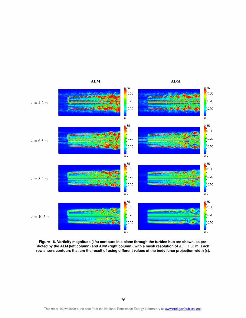
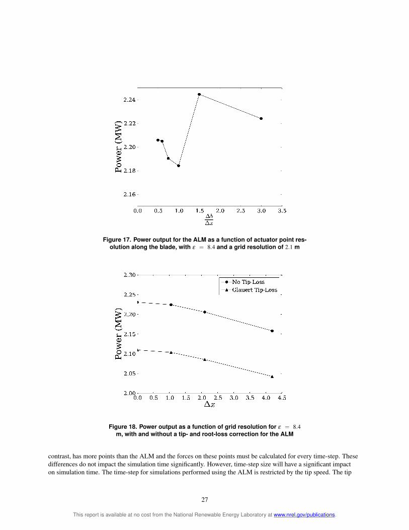
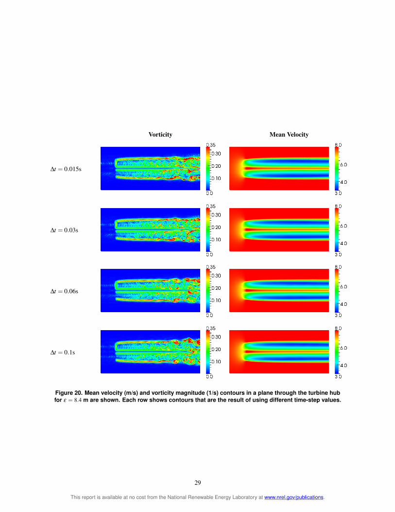
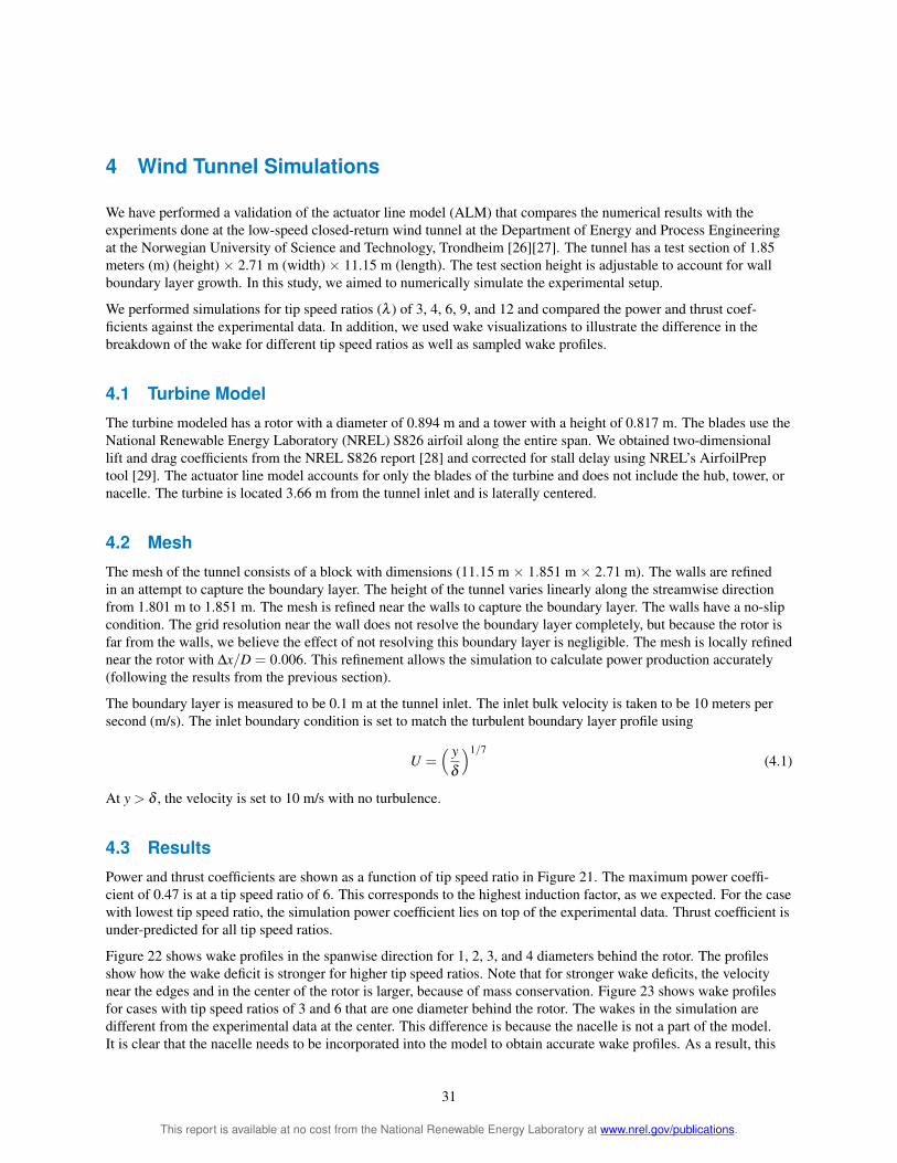
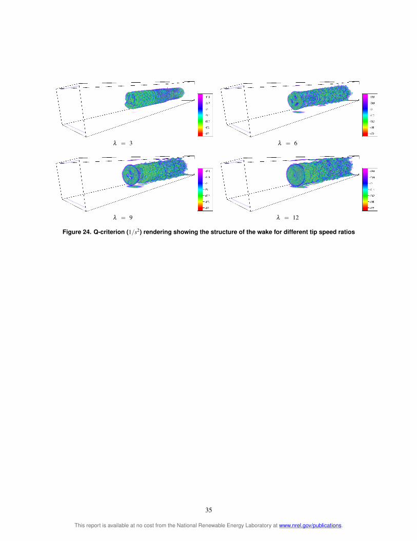
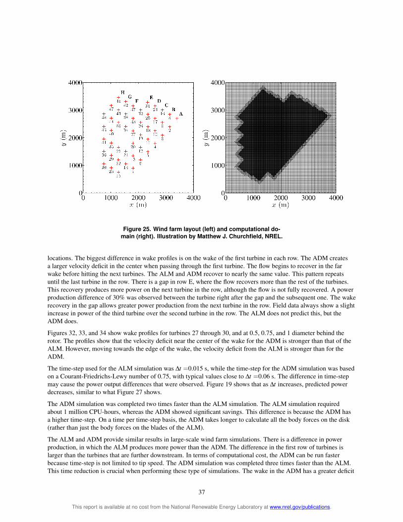

Row A Row B
Row C Row D
Row E Row F
Row G Row H
macrFigure 26 Ten minute average power produced by each turbine Pi normalized by the power of the first turbine in the row Average over one year of field data is shown for rows B-D
39
This report is available at no cost from the National Renewable Energy Laboratory at wwwnrelgovpublications
Row A Row B
Row C Row D
Row E Row F
Row G Row H
Figure 27 Power produced by each turbine
40
This report is available at no cost from the National Renewable Energy Laboratory at wwwnrelgovpublications
ADM ALM
Figure 28 Mean velocity (ms) contours at hub height for ADM (left) and ALM (right)
Figure 29 Mean velocity difference (ms) between ALM and ADM (ALM-ADM)
41
This report is available at no cost from the National Renewable Energy Laboratory at wwwnrelgovpublications
Row C Row E
yR = 0
yR = 025
yR = 05
yR = 075
yR = 1
Figure 30 Mean streamwise velocity profiles at hub height along rows C and E at various horizontal locations outboard of hub ranging from hub to blade tip
Turbine 30 Turbine 29
Turbine 28 Turbine 27
Figure 31 Mean velocity in the cross stream direction at one-fourth diameter behind the rotor for turbines in row D
42
This report is available at no cost from the National Renewable Energy Laboratory at wwwnrelgovpublications
Turbine 30 Turbine 29
Turbine 28 Turbine 27
Figure 32 Mean velocity in the cross stream direction at one-half diameter behind the rotor for turbines in row D
Turbine 30 Turbine 29
Turbine 28 Turbine 27
Figure 33 Mean velocity in the cross stream direction at three-fourths diameter behind the rotor for turbines in row D
43
This report is available at no cost from the National Renewable Energy Laboratory at wwwnrelgovpublications
Turbine 30 Turbine 29
Turbine 28 Turbine 27
Figure 34 Mean velocity in the cross stream direction at 1 diameter behind the rotor for turbines in row D
Turbine 30 Turbine 29
Turbine 28 Turbine 27
Figure 35 Mean velocity in the cross stream direction at 3 diameters behind the rotor for turbines in row D
44
This report is available at no cost from the National Renewable Energy Laboratory at wwwnrelgovpublications
Turbine 30 Turbine 29
Turbine 28 Turbine 27
Figure 36 Mean velocity in the cross stream direction at 4 diameters behind the rotor for turbines in row D
45
This report is available at no cost from the National Renewable Energy Laboratory at wwwnrelgovpublications
6 Conclusion and Future Work
The actuator line model (ALM) and actuator disk model (ADM) are a suitable representation of a wind turbine when using numerical simulations of fluid flows The models do not require that the full geometry of the blades be resolved and in which case model them as a set of points in the flow The ALM models the blades as a set of points along each blade axis whereas the ADM models the rotor as a disk with points that represent sections of the disk
The ADM and ALM provide very similar results in simulations with uniform inflow There is a clear grid depenshydence on power production and wake profiles of the ADM and ALM As the grid is refined the predicted power increases for both models Using a Glauert tip-loss correction with the ALM decreases the power production The number of actuator points in the ALM should be adequate to account for all the sections of the blade and provide smooth changes between them We recommend using a value smaller than ΔbΔx = 075 Mean wake profiles are similar for both the ADM and ALM
A Gaussian function was introduced to avoid numerical instabilities that are caused by the application of forces on discrete sections of the blade The width of the function was determined by the ε parameter This parameter played an important role in the models studied We observed that a parameter closest to the characteristic length of the blade section yielded the best results As the width of the projection function is decreased both the ALM and ADM predicted power decreases but never converges upon a value A specific value of epsilon allows agreement with blade-element momentum theory predictions However the ε parameter must be higher than 2Δx to avoid numerical instabilities in the solver
The ALM resolves the flow structures that are caused by the presence of individual blades which the ADM does not The ALM matches the physics more closely because it captures the root- and tip-vortices which the ADM does not Also the ALM is able to capture helical and asymmetric structures across the wake which caused asymmetric roll-up of Kelvin-Helmholtz-like instabilities in the wakersquos outer shear layer The ALM captures the vortical structures in the near wake ADM provides good results in the far wake but does not produce the vortical structures near the rotor If simulations are intended to determine the far wake effects the ADM should provide reasonable results
We used the ALM to validate a small-scale wind tunnel experiment and compared the structure of the wake for different tip speed ratios We observed that as the tip speed ratio is higher the breakdown of the wake occurs faster leaving a wider wake for larger tip speed ratios The tunnel walls play an important role in the simulation as the wake interacts with the walls The blockage effect of the turbine makes the reference velocity of the tunnel higher near the rotor than on the inlet
When performing large-scale wind farm simulations we found that the models perform well ALM produces slightly more power than ADM under atmospheric boundary layer conditions It is still unknown why this occurs but it is possible that the difference is caused by the time-step difference in the simulations The wake of the ADM is different from that of the ALM The ADM wake has a stronger wake deficit near the center whereas the ALM has a stronger wake deficit near the edges Wake profiles are similar but we observed that the greatest difference in the near wake primarily in the first row of turbines
46
This report is available at no cost from the National Renewable Energy Laboratory at wwwnrelgovpublications
Bibliography
[1] JN Soslashrensen Aerodynamics aspects of wind energy conversion 43427ndash448 September 2010
[2] T Burton D Sharpe N Jenkins and E Bossanyi Aerodynamics of Horizontal-Axis Wind Turbines pages 41ndash172 John Wiley amp Sons Ltd 2002
[3] JF Manwell JG McGowan and AL Rogers Wind Energy Explained Theory Design and Application Wiley 2010
[4] B Sanderse SP van der Pijl and B Koren Review of computational fluid dynamics for wind turbine wake aerodynamics Wind Energy 14 2011
[5] F Porteacute-Agel H Lu and YT Wu A Large-Eddy simulation framework for wind energy applications The Fifth International Symposium on Computational Wind Engineering (CWE2010) Chapel Hill North Carolina USA May 23-27 2010
[6] M Calaf C Meneveau and J Meyers Large eddy simulation study of fully developed wind-turbine array boundary layers Physics of Fluids 22(1)015110 2010
[7] N Troldborg JN Soslashrensen and R Mikkelsen Numerical simulations of wake charasteristics of a wind turbine in uniform flow 1386ndash99 2009
[8] T Phuoc Aeacuterodynamique instationnaire turbulente - aspects numeacuteriques et expeacuterimentaux Journeacute theacutematique DRET 1994
[9] N Troldborg Actuator Line Modeling of Wind Turbine Wakes PhD thesis Technical University of Denmark Lyngby Denmark 2008
[10] I Ammara C Leclerc and C Masson A viscous three-dimensional differentialactuator-disk method for the aerodynamic analysis of wind farms Journal of Solar Energy Engineering 124(4)345ndash356 2002
[11] A Jimenez A Crespo E Migoya and J Garcia Advances in large-eddy simulation of a wind turbine wake Journal of Physics Conference Series 75(1)012041 2007
[12] C Masson A Smaiumlli and C Leclerc Aerodynamic analysis of hawts operating in unsteady conditions Wind Energy 4(1)1ndash22 2001
[13] R Mikkelsen JN Soslashrensen and WZ Shen Modelling and analysis of the flow field around a coned rotor Wind Energy 4(3)121ndash135 2001
[14] JN Soslashrensen and WZ Shen Numerical modeling of wind turbine wakes Journal of Fluids Engineering 124(2)393ndash399 June 2002
[15] SSA Ivanell JN Soslashrensen R Mikkelsen and D Henningson Analysis of numerically generated wake structures Wind Energy 12(1)63ndash80 2009
[16] R Mikkelsen JN Soslashrensen S Oslashye and N Troldborg Analysis of power enhancement for a row of wind turbines using the actuator line technique Journal of Physics Conference Series ndash The Science of Making Torque from Wind 75(012044) 2007
[17] R Mikkelsen Actuator Disc Methods Applied to Wind Turbines PhD thesis Technical University of Denmark Mechanical Engineering Department 2003
[18] WZ Shen JH Zhang and JN Soslashrensen The actuator surface model A new navierndashstokes based model for rotor computations Journal of Solar Energy Engineering 131(1)011002 2009
47
This report is available at no cost from the National Renewable Energy Laboratory at wwwnrelgovpublications
[19] I Dobrev F Massouh and M Rapin Actuator surface hybrid model Journal of Physics Conference Series 75(1)012019 2007
[20] CS Watters and C Masson Modeling of lifting-device aerodynamics using the actuator surface concept International Journal for Numerical Methods in Fluids 62(11)1264ndash1298 2010
[21] OpenFOAM Ver 171 [available online] Silicon Graphics International Corporation (SGI) URL httpwwwopenfoamorgarchive171download [accessed 13 December 2011]
[22] J Smagorinsky General circulation experiments with the primitive equations Monthly Weather Review 9199ndash164 1963
[23] MJ Buhl WT_Perf Userrsquos Guide National Renewable Energy Laboratory 2004
[24] H Glauert Airplane Propellers pages 251ndash268 Dover New York 1985
[25] J Jonkman S Butterfield W Musial and G Scott Definition of a 5-MW reference wind turbine for offshore system development Technical Report NRELTP-500-38060
[26] MS Adaramola and P-A Krogstad Experimental investigation of wake effects on wind turbine performance Renewable Energy 362078ndash2086 2011
[27] P-A Krogstad and JA Lund An experimental and numerical study of the performance of a model turbine Wind Energy 2011
[28] DM Somers The S825 and S826 Airfoils Period of Performance 1994ndash1995 The S825 and S826 Airfoils Technical Report January 2005
[29] NWTC Design Codes (AirfoilPrep by Dr Craig Hansen) httpwindnrelgovdesigncodespreprocessorsairfoilprep [Accessed 21 February 2012]
[30] JCR Hunt AA Wray and P Moin Eddies streams and convergence zones in turbulent flows (1970) 1988
[31] MJ Churchfield S Lee P Moriarty LA Martiacutenez S Leonardi G Vijayakumar and JG Brasseur A large-eddy simulation of wind-plant aerodynamics 50th AIAA Aerospace Sciences Meeting Nashville Tennessee USA 2012
[32] MJ Churchield A Method for Designing Generic Wind Turbine Models Representative of Real Turbines and Generic Siemens SWT-23-93 and Vestas V80 Specifications National Renewable Energy Laboratory 2012
48
This report is available at no cost from the National Renewable Energy Laboratory at wwwnrelgovpublications
- Literature Review
-
- Introduction
- Basics of Wind Turbine Aerodynamics
- Wind Turbine Computational Fluid Dynamics
- Atmospheric Boundary Layer Simulations
- Actuator Disc Model (ADM)
- Actuator Line Model (ALM)
- Actuator Surface Model (ASM)
- Comparison Between ADM and ALM
- Conclusions
-
- Actuator Turbine Model Implementation
-
- Actuator Line Model
- Actuator Disk Model
- Numerical Method
-
- Actuator Disk and Actuator Line Models in Uniform Nonturbulent Inflow
-
- Five Megawatt Reference Turbine
- Actuator Line Model
- Actuator Disk Model
- Actuator Points
- Tip Loss Correction
- Time-step
- Comparison
- The Parameter
-
- Wind Tunnel Simulations
-
- Turbine Model
- Mesh
- Results
-
- Wind Farm Simulation
-
- Introduction
- Results
-
- Conclusion and Future Work
- Bibliography
-
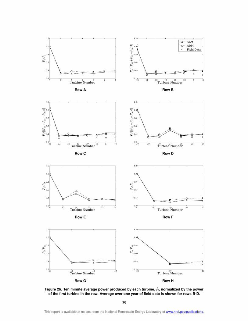
Row A Row B
Row C Row D
Row E Row F
Row G Row H
Figure 27 Power produced by each turbine
40
This report is available at no cost from the National Renewable Energy Laboratory at wwwnrelgovpublications
ADM ALM
Figure 28 Mean velocity (ms) contours at hub height for ADM (left) and ALM (right)
Figure 29 Mean velocity difference (ms) between ALM and ADM (ALM-ADM)
41
This report is available at no cost from the National Renewable Energy Laboratory at wwwnrelgovpublications
Row C Row E
yR = 0
yR = 025
yR = 05
yR = 075
yR = 1
Figure 30 Mean streamwise velocity profiles at hub height along rows C and E at various horizontal locations outboard of hub ranging from hub to blade tip
Turbine 30 Turbine 29
Turbine 28 Turbine 27
Figure 31 Mean velocity in the cross stream direction at one-fourth diameter behind the rotor for turbines in row D
42
This report is available at no cost from the National Renewable Energy Laboratory at wwwnrelgovpublications
Turbine 30 Turbine 29
Turbine 28 Turbine 27
Figure 32 Mean velocity in the cross stream direction at one-half diameter behind the rotor for turbines in row D
Turbine 30 Turbine 29
Turbine 28 Turbine 27
Figure 33 Mean velocity in the cross stream direction at three-fourths diameter behind the rotor for turbines in row D
43
This report is available at no cost from the National Renewable Energy Laboratory at wwwnrelgovpublications
Turbine 30 Turbine 29
Turbine 28 Turbine 27
Figure 34 Mean velocity in the cross stream direction at 1 diameter behind the rotor for turbines in row D
Turbine 30 Turbine 29
Turbine 28 Turbine 27
Figure 35 Mean velocity in the cross stream direction at 3 diameters behind the rotor for turbines in row D
44
This report is available at no cost from the National Renewable Energy Laboratory at wwwnrelgovpublications
Turbine 30 Turbine 29
Turbine 28 Turbine 27
Figure 36 Mean velocity in the cross stream direction at 4 diameters behind the rotor for turbines in row D
45
This report is available at no cost from the National Renewable Energy Laboratory at wwwnrelgovpublications
6 Conclusion and Future Work
The actuator line model (ALM) and actuator disk model (ADM) are a suitable representation of a wind turbine when using numerical simulations of fluid flows The models do not require that the full geometry of the blades be resolved and in which case model them as a set of points in the flow The ALM models the blades as a set of points along each blade axis whereas the ADM models the rotor as a disk with points that represent sections of the disk
The ADM and ALM provide very similar results in simulations with uniform inflow There is a clear grid depenshydence on power production and wake profiles of the ADM and ALM As the grid is refined the predicted power increases for both models Using a Glauert tip-loss correction with the ALM decreases the power production The number of actuator points in the ALM should be adequate to account for all the sections of the blade and provide smooth changes between them We recommend using a value smaller than ΔbΔx = 075 Mean wake profiles are similar for both the ADM and ALM
A Gaussian function was introduced to avoid numerical instabilities that are caused by the application of forces on discrete sections of the blade The width of the function was determined by the ε parameter This parameter played an important role in the models studied We observed that a parameter closest to the characteristic length of the blade section yielded the best results As the width of the projection function is decreased both the ALM and ADM predicted power decreases but never converges upon a value A specific value of epsilon allows agreement with blade-element momentum theory predictions However the ε parameter must be higher than 2Δx to avoid numerical instabilities in the solver
The ALM resolves the flow structures that are caused by the presence of individual blades which the ADM does not The ALM matches the physics more closely because it captures the root- and tip-vortices which the ADM does not Also the ALM is able to capture helical and asymmetric structures across the wake which caused asymmetric roll-up of Kelvin-Helmholtz-like instabilities in the wakersquos outer shear layer The ALM captures the vortical structures in the near wake ADM provides good results in the far wake but does not produce the vortical structures near the rotor If simulations are intended to determine the far wake effects the ADM should provide reasonable results
We used the ALM to validate a small-scale wind tunnel experiment and compared the structure of the wake for different tip speed ratios We observed that as the tip speed ratio is higher the breakdown of the wake occurs faster leaving a wider wake for larger tip speed ratios The tunnel walls play an important role in the simulation as the wake interacts with the walls The blockage effect of the turbine makes the reference velocity of the tunnel higher near the rotor than on the inlet
When performing large-scale wind farm simulations we found that the models perform well ALM produces slightly more power than ADM under atmospheric boundary layer conditions It is still unknown why this occurs but it is possible that the difference is caused by the time-step difference in the simulations The wake of the ADM is different from that of the ALM The ADM wake has a stronger wake deficit near the center whereas the ALM has a stronger wake deficit near the edges Wake profiles are similar but we observed that the greatest difference in the near wake primarily in the first row of turbines
46
This report is available at no cost from the National Renewable Energy Laboratory at wwwnrelgovpublications
Bibliography
[1] JN Soslashrensen Aerodynamics aspects of wind energy conversion 43427ndash448 September 2010
[2] T Burton D Sharpe N Jenkins and E Bossanyi Aerodynamics of Horizontal-Axis Wind Turbines pages 41ndash172 John Wiley amp Sons Ltd 2002
[3] JF Manwell JG McGowan and AL Rogers Wind Energy Explained Theory Design and Application Wiley 2010
[4] B Sanderse SP van der Pijl and B Koren Review of computational fluid dynamics for wind turbine wake aerodynamics Wind Energy 14 2011
[5] F Porteacute-Agel H Lu and YT Wu A Large-Eddy simulation framework for wind energy applications The Fifth International Symposium on Computational Wind Engineering (CWE2010) Chapel Hill North Carolina USA May 23-27 2010
[6] M Calaf C Meneveau and J Meyers Large eddy simulation study of fully developed wind-turbine array boundary layers Physics of Fluids 22(1)015110 2010
[7] N Troldborg JN Soslashrensen and R Mikkelsen Numerical simulations of wake charasteristics of a wind turbine in uniform flow 1386ndash99 2009
[8] T Phuoc Aeacuterodynamique instationnaire turbulente - aspects numeacuteriques et expeacuterimentaux Journeacute theacutematique DRET 1994
[9] N Troldborg Actuator Line Modeling of Wind Turbine Wakes PhD thesis Technical University of Denmark Lyngby Denmark 2008
[10] I Ammara C Leclerc and C Masson A viscous three-dimensional differentialactuator-disk method for the aerodynamic analysis of wind farms Journal of Solar Energy Engineering 124(4)345ndash356 2002
[11] A Jimenez A Crespo E Migoya and J Garcia Advances in large-eddy simulation of a wind turbine wake Journal of Physics Conference Series 75(1)012041 2007
[12] C Masson A Smaiumlli and C Leclerc Aerodynamic analysis of hawts operating in unsteady conditions Wind Energy 4(1)1ndash22 2001
[13] R Mikkelsen JN Soslashrensen and WZ Shen Modelling and analysis of the flow field around a coned rotor Wind Energy 4(3)121ndash135 2001
[14] JN Soslashrensen and WZ Shen Numerical modeling of wind turbine wakes Journal of Fluids Engineering 124(2)393ndash399 June 2002
[15] SSA Ivanell JN Soslashrensen R Mikkelsen and D Henningson Analysis of numerically generated wake structures Wind Energy 12(1)63ndash80 2009
[16] R Mikkelsen JN Soslashrensen S Oslashye and N Troldborg Analysis of power enhancement for a row of wind turbines using the actuator line technique Journal of Physics Conference Series ndash The Science of Making Torque from Wind 75(012044) 2007
[17] R Mikkelsen Actuator Disc Methods Applied to Wind Turbines PhD thesis Technical University of Denmark Mechanical Engineering Department 2003
[18] WZ Shen JH Zhang and JN Soslashrensen The actuator surface model A new navierndashstokes based model for rotor computations Journal of Solar Energy Engineering 131(1)011002 2009
47
This report is available at no cost from the National Renewable Energy Laboratory at wwwnrelgovpublications
[19] I Dobrev F Massouh and M Rapin Actuator surface hybrid model Journal of Physics Conference Series 75(1)012019 2007
[20] CS Watters and C Masson Modeling of lifting-device aerodynamics using the actuator surface concept International Journal for Numerical Methods in Fluids 62(11)1264ndash1298 2010
[21] OpenFOAM Ver 171 [available online] Silicon Graphics International Corporation (SGI) URL httpwwwopenfoamorgarchive171download [accessed 13 December 2011]
[22] J Smagorinsky General circulation experiments with the primitive equations Monthly Weather Review 9199ndash164 1963
[23] MJ Buhl WT_Perf Userrsquos Guide National Renewable Energy Laboratory 2004
[24] H Glauert Airplane Propellers pages 251ndash268 Dover New York 1985
[25] J Jonkman S Butterfield W Musial and G Scott Definition of a 5-MW reference wind turbine for offshore system development Technical Report NRELTP-500-38060
[26] MS Adaramola and P-A Krogstad Experimental investigation of wake effects on wind turbine performance Renewable Energy 362078ndash2086 2011
[27] P-A Krogstad and JA Lund An experimental and numerical study of the performance of a model turbine Wind Energy 2011
[28] DM Somers The S825 and S826 Airfoils Period of Performance 1994ndash1995 The S825 and S826 Airfoils Technical Report January 2005
[29] NWTC Design Codes (AirfoilPrep by Dr Craig Hansen) httpwindnrelgovdesigncodespreprocessorsairfoilprep [Accessed 21 February 2012]
[30] JCR Hunt AA Wray and P Moin Eddies streams and convergence zones in turbulent flows (1970) 1988
[31] MJ Churchfield S Lee P Moriarty LA Martiacutenez S Leonardi G Vijayakumar and JG Brasseur A large-eddy simulation of wind-plant aerodynamics 50th AIAA Aerospace Sciences Meeting Nashville Tennessee USA 2012
[32] MJ Churchield A Method for Designing Generic Wind Turbine Models Representative of Real Turbines and Generic Siemens SWT-23-93 and Vestas V80 Specifications National Renewable Energy Laboratory 2012
48
This report is available at no cost from the National Renewable Energy Laboratory at wwwnrelgovpublications
- Literature Review
-
- Introduction
- Basics of Wind Turbine Aerodynamics
- Wind Turbine Computational Fluid Dynamics
- Atmospheric Boundary Layer Simulations
- Actuator Disc Model (ADM)
- Actuator Line Model (ALM)
- Actuator Surface Model (ASM)
- Comparison Between ADM and ALM
- Conclusions
-
- Actuator Turbine Model Implementation
-
- Actuator Line Model
- Actuator Disk Model
- Numerical Method
-
- Actuator Disk and Actuator Line Models in Uniform Nonturbulent Inflow
-
- Five Megawatt Reference Turbine
- Actuator Line Model
- Actuator Disk Model
- Actuator Points
- Tip Loss Correction
- Time-step
- Comparison
- The Parameter
-
- Wind Tunnel Simulations
-
- Turbine Model
- Mesh
- Results
-
- Wind Farm Simulation
-
- Introduction
- Results
-
- Conclusion and Future Work
- Bibliography
-
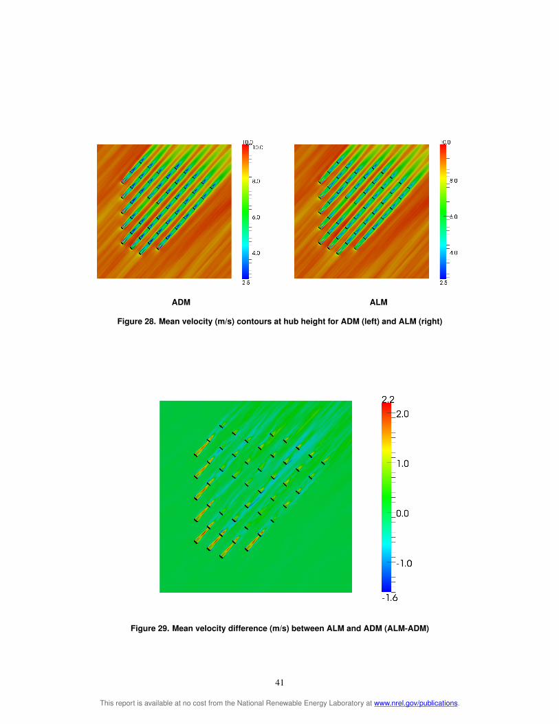
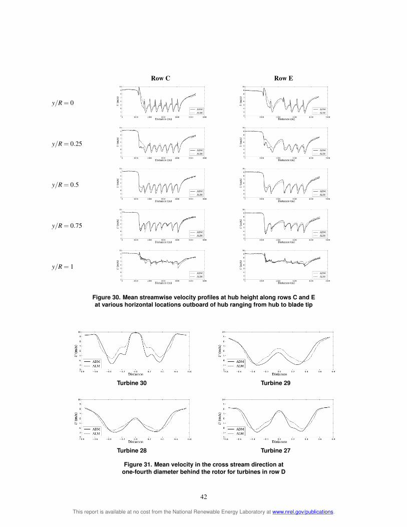
Turbine 30 Turbine 29
Turbine 28 Turbine 27
Figure 34 Mean velocity in the cross stream direction at 1 diameter behind the rotor for turbines in row D
Turbine 30 Turbine 29
Turbine 28 Turbine 27
Figure 35 Mean velocity in the cross stream direction at 3 diameters behind the rotor for turbines in row D
44
This report is available at no cost from the National Renewable Energy Laboratory at wwwnrelgovpublications
Turbine 30 Turbine 29
Turbine 28 Turbine 27
Figure 36 Mean velocity in the cross stream direction at 4 diameters behind the rotor for turbines in row D
45
This report is available at no cost from the National Renewable Energy Laboratory at wwwnrelgovpublications
6 Conclusion and Future Work
The actuator line model (ALM) and actuator disk model (ADM) are a suitable representation of a wind turbine when using numerical simulations of fluid flows The models do not require that the full geometry of the blades be resolved and in which case model them as a set of points in the flow The ALM models the blades as a set of points along each blade axis whereas the ADM models the rotor as a disk with points that represent sections of the disk
The ADM and ALM provide very similar results in simulations with uniform inflow There is a clear grid depenshydence on power production and wake profiles of the ADM and ALM As the grid is refined the predicted power increases for both models Using a Glauert tip-loss correction with the ALM decreases the power production The number of actuator points in the ALM should be adequate to account for all the sections of the blade and provide smooth changes between them We recommend using a value smaller than ΔbΔx = 075 Mean wake profiles are similar for both the ADM and ALM
A Gaussian function was introduced to avoid numerical instabilities that are caused by the application of forces on discrete sections of the blade The width of the function was determined by the ε parameter This parameter played an important role in the models studied We observed that a parameter closest to the characteristic length of the blade section yielded the best results As the width of the projection function is decreased both the ALM and ADM predicted power decreases but never converges upon a value A specific value of epsilon allows agreement with blade-element momentum theory predictions However the ε parameter must be higher than 2Δx to avoid numerical instabilities in the solver
The ALM resolves the flow structures that are caused by the presence of individual blades which the ADM does not The ALM matches the physics more closely because it captures the root- and tip-vortices which the ADM does not Also the ALM is able to capture helical and asymmetric structures across the wake which caused asymmetric roll-up of Kelvin-Helmholtz-like instabilities in the wakersquos outer shear layer The ALM captures the vortical structures in the near wake ADM provides good results in the far wake but does not produce the vortical structures near the rotor If simulations are intended to determine the far wake effects the ADM should provide reasonable results
We used the ALM to validate a small-scale wind tunnel experiment and compared the structure of the wake for different tip speed ratios We observed that as the tip speed ratio is higher the breakdown of the wake occurs faster leaving a wider wake for larger tip speed ratios The tunnel walls play an important role in the simulation as the wake interacts with the walls The blockage effect of the turbine makes the reference velocity of the tunnel higher near the rotor than on the inlet
When performing large-scale wind farm simulations we found that the models perform well ALM produces slightly more power than ADM under atmospheric boundary layer conditions It is still unknown why this occurs but it is possible that the difference is caused by the time-step difference in the simulations The wake of the ADM is different from that of the ALM The ADM wake has a stronger wake deficit near the center whereas the ALM has a stronger wake deficit near the edges Wake profiles are similar but we observed that the greatest difference in the near wake primarily in the first row of turbines
46
This report is available at no cost from the National Renewable Energy Laboratory at wwwnrelgovpublications
Bibliography
[1] JN Soslashrensen Aerodynamics aspects of wind energy conversion 43427ndash448 September 2010
[2] T Burton D Sharpe N Jenkins and E Bossanyi Aerodynamics of Horizontal-Axis Wind Turbines pages 41ndash172 John Wiley amp Sons Ltd 2002
[3] JF Manwell JG McGowan and AL Rogers Wind Energy Explained Theory Design and Application Wiley 2010
[4] B Sanderse SP van der Pijl and B Koren Review of computational fluid dynamics for wind turbine wake aerodynamics Wind Energy 14 2011
[5] F Porteacute-Agel H Lu and YT Wu A Large-Eddy simulation framework for wind energy applications The Fifth International Symposium on Computational Wind Engineering (CWE2010) Chapel Hill North Carolina USA May 23-27 2010
[6] M Calaf C Meneveau and J Meyers Large eddy simulation study of fully developed wind-turbine array boundary layers Physics of Fluids 22(1)015110 2010
[7] N Troldborg JN Soslashrensen and R Mikkelsen Numerical simulations of wake charasteristics of a wind turbine in uniform flow 1386ndash99 2009
[8] T Phuoc Aeacuterodynamique instationnaire turbulente - aspects numeacuteriques et expeacuterimentaux Journeacute theacutematique DRET 1994
[9] N Troldborg Actuator Line Modeling of Wind Turbine Wakes PhD thesis Technical University of Denmark Lyngby Denmark 2008
[10] I Ammara C Leclerc and C Masson A viscous three-dimensional differentialactuator-disk method for the aerodynamic analysis of wind farms Journal of Solar Energy Engineering 124(4)345ndash356 2002
[11] A Jimenez A Crespo E Migoya and J Garcia Advances in large-eddy simulation of a wind turbine wake Journal of Physics Conference Series 75(1)012041 2007
[12] C Masson A Smaiumlli and C Leclerc Aerodynamic analysis of hawts operating in unsteady conditions Wind Energy 4(1)1ndash22 2001
[13] R Mikkelsen JN Soslashrensen and WZ Shen Modelling and analysis of the flow field around a coned rotor Wind Energy 4(3)121ndash135 2001
[14] JN Soslashrensen and WZ Shen Numerical modeling of wind turbine wakes Journal of Fluids Engineering 124(2)393ndash399 June 2002
[15] SSA Ivanell JN Soslashrensen R Mikkelsen and D Henningson Analysis of numerically generated wake structures Wind Energy 12(1)63ndash80 2009
[16] R Mikkelsen JN Soslashrensen S Oslashye and N Troldborg Analysis of power enhancement for a row of wind turbines using the actuator line technique Journal of Physics Conference Series ndash The Science of Making Torque from Wind 75(012044) 2007
[17] R Mikkelsen Actuator Disc Methods Applied to Wind Turbines PhD thesis Technical University of Denmark Mechanical Engineering Department 2003
[18] WZ Shen JH Zhang and JN Soslashrensen The actuator surface model A new navierndashstokes based model for rotor computations Journal of Solar Energy Engineering 131(1)011002 2009
47
This report is available at no cost from the National Renewable Energy Laboratory at wwwnrelgovpublications
[19] I Dobrev F Massouh and M Rapin Actuator surface hybrid model Journal of Physics Conference Series 75(1)012019 2007
[20] CS Watters and C Masson Modeling of lifting-device aerodynamics using the actuator surface concept International Journal for Numerical Methods in Fluids 62(11)1264ndash1298 2010
[21] OpenFOAM Ver 171 [available online] Silicon Graphics International Corporation (SGI) URL httpwwwopenfoamorgarchive171download [accessed 13 December 2011]
[22] J Smagorinsky General circulation experiments with the primitive equations Monthly Weather Review 9199ndash164 1963
[23] MJ Buhl WT_Perf Userrsquos Guide National Renewable Energy Laboratory 2004
[24] H Glauert Airplane Propellers pages 251ndash268 Dover New York 1985
[25] J Jonkman S Butterfield W Musial and G Scott Definition of a 5-MW reference wind turbine for offshore system development Technical Report NRELTP-500-38060
[26] MS Adaramola and P-A Krogstad Experimental investigation of wake effects on wind turbine performance Renewable Energy 362078ndash2086 2011
[27] P-A Krogstad and JA Lund An experimental and numerical study of the performance of a model turbine Wind Energy 2011
[28] DM Somers The S825 and S826 Airfoils Period of Performance 1994ndash1995 The S825 and S826 Airfoils Technical Report January 2005
[29] NWTC Design Codes (AirfoilPrep by Dr Craig Hansen) httpwindnrelgovdesigncodespreprocessorsairfoilprep [Accessed 21 February 2012]
[30] JCR Hunt AA Wray and P Moin Eddies streams and convergence zones in turbulent flows (1970) 1988
[31] MJ Churchfield S Lee P Moriarty LA Martiacutenez S Leonardi G Vijayakumar and JG Brasseur A large-eddy simulation of wind-plant aerodynamics 50th AIAA Aerospace Sciences Meeting Nashville Tennessee USA 2012
[32] MJ Churchield A Method for Designing Generic Wind Turbine Models Representative of Real Turbines and Generic Siemens SWT-23-93 and Vestas V80 Specifications National Renewable Energy Laboratory 2012
48
This report is available at no cost from the National Renewable Energy Laboratory at wwwnrelgovpublications
- Literature Review
-
- Introduction
- Basics of Wind Turbine Aerodynamics
- Wind Turbine Computational Fluid Dynamics
- Atmospheric Boundary Layer Simulations
- Actuator Disc Model (ADM)
- Actuator Line Model (ALM)
- Actuator Surface Model (ASM)
- Comparison Between ADM and ALM
- Conclusions
-
- Actuator Turbine Model Implementation
-
- Actuator Line Model
- Actuator Disk Model
- Numerical Method
-
- Actuator Disk and Actuator Line Models in Uniform Nonturbulent Inflow
-
- Five Megawatt Reference Turbine
- Actuator Line Model
- Actuator Disk Model
- Actuator Points
- Tip Loss Correction
- Time-step
- Comparison
- The Parameter
-
- Wind Tunnel Simulations
-
- Turbine Model
- Mesh
- Results
-
- Wind Farm Simulation
-
- Introduction
- Results
-
- Conclusion and Future Work
- Bibliography
-
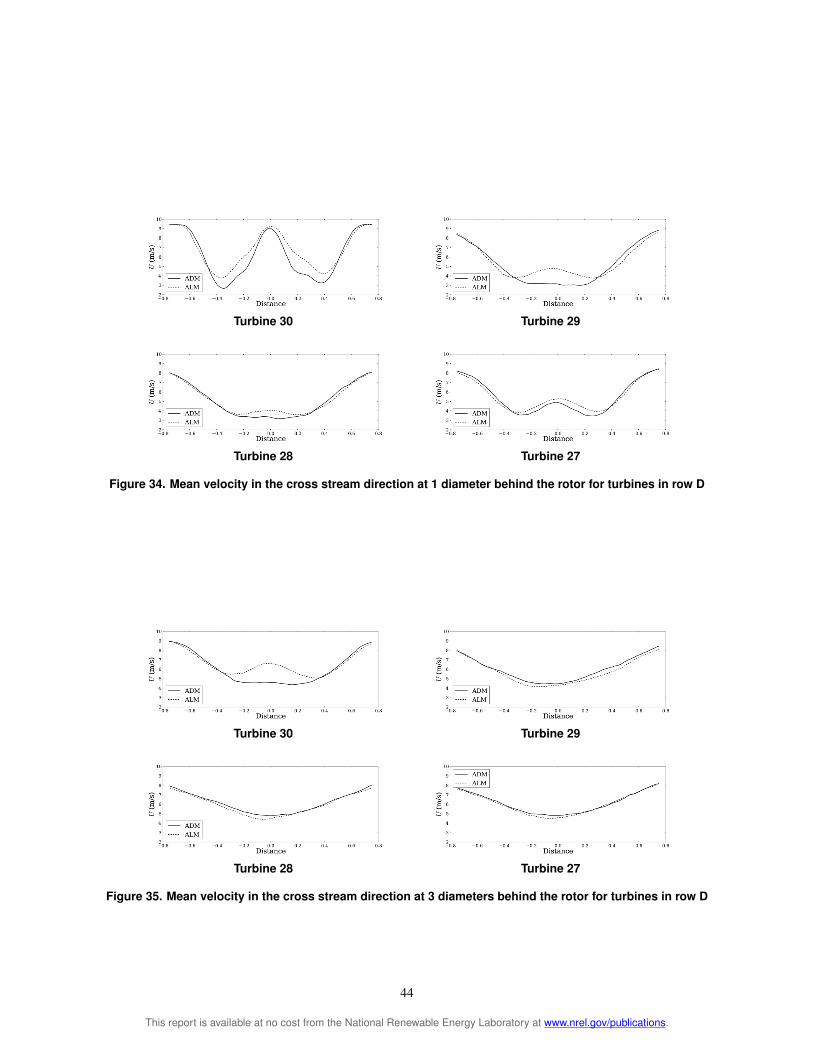
Turbine 30 Turbine 29
Turbine 28 Turbine 27
Figure 36 Mean velocity in the cross stream direction at 4 diameters behind the rotor for turbines in row D
45
This report is available at no cost from the National Renewable Energy Laboratory at wwwnrelgovpublications
6 Conclusion and Future Work
The actuator line model (ALM) and actuator disk model (ADM) are a suitable representation of a wind turbine when using numerical simulations of fluid flows The models do not require that the full geometry of the blades be resolved and in which case model them as a set of points in the flow The ALM models the blades as a set of points along each blade axis whereas the ADM models the rotor as a disk with points that represent sections of the disk
The ADM and ALM provide very similar results in simulations with uniform inflow There is a clear grid depenshydence on power production and wake profiles of the ADM and ALM As the grid is refined the predicted power increases for both models Using a Glauert tip-loss correction with the ALM decreases the power production The number of actuator points in the ALM should be adequate to account for all the sections of the blade and provide smooth changes between them We recommend using a value smaller than ΔbΔx = 075 Mean wake profiles are similar for both the ADM and ALM
A Gaussian function was introduced to avoid numerical instabilities that are caused by the application of forces on discrete sections of the blade The width of the function was determined by the ε parameter This parameter played an important role in the models studied We observed that a parameter closest to the characteristic length of the blade section yielded the best results As the width of the projection function is decreased both the ALM and ADM predicted power decreases but never converges upon a value A specific value of epsilon allows agreement with blade-element momentum theory predictions However the ε parameter must be higher than 2Δx to avoid numerical instabilities in the solver
The ALM resolves the flow structures that are caused by the presence of individual blades which the ADM does not The ALM matches the physics more closely because it captures the root- and tip-vortices which the ADM does not Also the ALM is able to capture helical and asymmetric structures across the wake which caused asymmetric roll-up of Kelvin-Helmholtz-like instabilities in the wakersquos outer shear layer The ALM captures the vortical structures in the near wake ADM provides good results in the far wake but does not produce the vortical structures near the rotor If simulations are intended to determine the far wake effects the ADM should provide reasonable results
We used the ALM to validate a small-scale wind tunnel experiment and compared the structure of the wake for different tip speed ratios We observed that as the tip speed ratio is higher the breakdown of the wake occurs faster leaving a wider wake for larger tip speed ratios The tunnel walls play an important role in the simulation as the wake interacts with the walls The blockage effect of the turbine makes the reference velocity of the tunnel higher near the rotor than on the inlet
When performing large-scale wind farm simulations we found that the models perform well ALM produces slightly more power than ADM under atmospheric boundary layer conditions It is still unknown why this occurs but it is possible that the difference is caused by the time-step difference in the simulations The wake of the ADM is different from that of the ALM The ADM wake has a stronger wake deficit near the center whereas the ALM has a stronger wake deficit near the edges Wake profiles are similar but we observed that the greatest difference in the near wake primarily in the first row of turbines
46
This report is available at no cost from the National Renewable Energy Laboratory at wwwnrelgovpublications
Bibliography
[1] JN Soslashrensen Aerodynamics aspects of wind energy conversion 43427ndash448 September 2010
[2] T Burton D Sharpe N Jenkins and E Bossanyi Aerodynamics of Horizontal-Axis Wind Turbines pages 41ndash172 John Wiley amp Sons Ltd 2002
[3] JF Manwell JG McGowan and AL Rogers Wind Energy Explained Theory Design and Application Wiley 2010
[4] B Sanderse SP van der Pijl and B Koren Review of computational fluid dynamics for wind turbine wake aerodynamics Wind Energy 14 2011
[5] F Porteacute-Agel H Lu and YT Wu A Large-Eddy simulation framework for wind energy applications The Fifth International Symposium on Computational Wind Engineering (CWE2010) Chapel Hill North Carolina USA May 23-27 2010
[6] M Calaf C Meneveau and J Meyers Large eddy simulation study of fully developed wind-turbine array boundary layers Physics of Fluids 22(1)015110 2010
[7] N Troldborg JN Soslashrensen and R Mikkelsen Numerical simulations of wake charasteristics of a wind turbine in uniform flow 1386ndash99 2009
[8] T Phuoc Aeacuterodynamique instationnaire turbulente - aspects numeacuteriques et expeacuterimentaux Journeacute theacutematique DRET 1994
[9] N Troldborg Actuator Line Modeling of Wind Turbine Wakes PhD thesis Technical University of Denmark Lyngby Denmark 2008
[10] I Ammara C Leclerc and C Masson A viscous three-dimensional differentialactuator-disk method for the aerodynamic analysis of wind farms Journal of Solar Energy Engineering 124(4)345ndash356 2002
[11] A Jimenez A Crespo E Migoya and J Garcia Advances in large-eddy simulation of a wind turbine wake Journal of Physics Conference Series 75(1)012041 2007
[12] C Masson A Smaiumlli and C Leclerc Aerodynamic analysis of hawts operating in unsteady conditions Wind Energy 4(1)1ndash22 2001
[13] R Mikkelsen JN Soslashrensen and WZ Shen Modelling and analysis of the flow field around a coned rotor Wind Energy 4(3)121ndash135 2001
[14] JN Soslashrensen and WZ Shen Numerical modeling of wind turbine wakes Journal of Fluids Engineering 124(2)393ndash399 June 2002
[15] SSA Ivanell JN Soslashrensen R Mikkelsen and D Henningson Analysis of numerically generated wake structures Wind Energy 12(1)63ndash80 2009
[16] R Mikkelsen JN Soslashrensen S Oslashye and N Troldborg Analysis of power enhancement for a row of wind turbines using the actuator line technique Journal of Physics Conference Series ndash The Science of Making Torque from Wind 75(012044) 2007
[17] R Mikkelsen Actuator Disc Methods Applied to Wind Turbines PhD thesis Technical University of Denmark Mechanical Engineering Department 2003
[18] WZ Shen JH Zhang and JN Soslashrensen The actuator surface model A new navierndashstokes based model for rotor computations Journal of Solar Energy Engineering 131(1)011002 2009
47
This report is available at no cost from the National Renewable Energy Laboratory at wwwnrelgovpublications
[19] I Dobrev F Massouh and M Rapin Actuator surface hybrid model Journal of Physics Conference Series 75(1)012019 2007
[20] CS Watters and C Masson Modeling of lifting-device aerodynamics using the actuator surface concept International Journal for Numerical Methods in Fluids 62(11)1264ndash1298 2010
[21] OpenFOAM Ver 171 [available online] Silicon Graphics International Corporation (SGI) URL httpwwwopenfoamorgarchive171download [accessed 13 December 2011]
[22] J Smagorinsky General circulation experiments with the primitive equations Monthly Weather Review 9199ndash164 1963
[23] MJ Buhl WT_Perf Userrsquos Guide National Renewable Energy Laboratory 2004
[24] H Glauert Airplane Propellers pages 251ndash268 Dover New York 1985
[25] J Jonkman S Butterfield W Musial and G Scott Definition of a 5-MW reference wind turbine for offshore system development Technical Report NRELTP-500-38060
[26] MS Adaramola and P-A Krogstad Experimental investigation of wake effects on wind turbine performance Renewable Energy 362078ndash2086 2011
[27] P-A Krogstad and JA Lund An experimental and numerical study of the performance of a model turbine Wind Energy 2011
[28] DM Somers The S825 and S826 Airfoils Period of Performance 1994ndash1995 The S825 and S826 Airfoils Technical Report January 2005
[29] NWTC Design Codes (AirfoilPrep by Dr Craig Hansen) httpwindnrelgovdesigncodespreprocessorsairfoilprep [Accessed 21 February 2012]
[30] JCR Hunt AA Wray and P Moin Eddies streams and convergence zones in turbulent flows (1970) 1988
[31] MJ Churchfield S Lee P Moriarty LA Martiacutenez S Leonardi G Vijayakumar and JG Brasseur A large-eddy simulation of wind-plant aerodynamics 50th AIAA Aerospace Sciences Meeting Nashville Tennessee USA 2012
[32] MJ Churchield A Method for Designing Generic Wind Turbine Models Representative of Real Turbines and Generic Siemens SWT-23-93 and Vestas V80 Specifications National Renewable Energy Laboratory 2012
48
This report is available at no cost from the National Renewable Energy Laboratory at wwwnrelgovpublications
- Literature Review
-
- Introduction
- Basics of Wind Turbine Aerodynamics
- Wind Turbine Computational Fluid Dynamics
- Atmospheric Boundary Layer Simulations
- Actuator Disc Model (ADM)
- Actuator Line Model (ALM)
- Actuator Surface Model (ASM)
- Comparison Between ADM and ALM
- Conclusions
-
- Actuator Turbine Model Implementation
-
- Actuator Line Model
- Actuator Disk Model
- Numerical Method
-
- Actuator Disk and Actuator Line Models in Uniform Nonturbulent Inflow
-
- Five Megawatt Reference Turbine
- Actuator Line Model
- Actuator Disk Model
- Actuator Points
- Tip Loss Correction
- Time-step
- Comparison
- The Parameter
-
- Wind Tunnel Simulations
-
- Turbine Model
- Mesh
- Results
-
- Wind Farm Simulation
-
- Introduction
- Results
-
- Conclusion and Future Work
- Bibliography
-
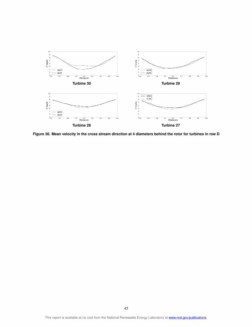