wind turbine controls for farm and offshore operation
TRANSCRIPT

University of Wisconsin MilwaukeeUWM Digital Commons
Theses and Dissertations
December 2013
Wind Turbine Controls for Farm and OffshoreOperationZhongzhou YangUniversity of Wisconsin-Milwaukee
Follow this and additional works at: https://dc.uwm.edu/etdPart of the Mechanical Engineering Commons, and the Oil, Gas, and Energy Commons
This Dissertation is brought to you for free and open access by UWM Digital Commons. It has been accepted for inclusion in Theses and Dissertationsby an authorized administrator of UWM Digital Commons. For more information, please contact [email protected].
Recommended CitationYang, Zhongzhou, "Wind Turbine Controls for Farm and Offshore Operation" (2013). Theses and Dissertations. 382.https://dc.uwm.edu/etd/382

WIND TURBINE CONTROLS FOR FARM AND
OFFSHORE OPERATION
by
Zhongzhou Yang
A Dissertation Submitted in
Partial Fulfillment of the
Requirements for the Degree of
Doctor of Philosophy
in Engineering
at
The University of Wisconsin-Milwaukee
December 2013

ABSTRACT
WIND TURBINE CONTROLS IN WIND FARM AND OFFSHORE OPERATION
by
Zhongzhou Yang
The University of Wisconsin-Milwaukee, 2013 Under Supervision of Professor Yaoyu Li and Dr. John E. Seem
Development of advanced control techniques is a critical measure for reducing the
cost of energy for wind power generation, in terms of both enhancing energy capture and
reducing fatigue load. There are two remarkable trends for wind energy. First, more and
more large wind farms are developed in order to reduce the unit-power cost in installation,
operation, maintenance and transmission. Second, offshore wind energy has received
significant attention when the scarcity of land resource has appeared to be a major
bottleneck for next level of wind penetration, especially for Europe and Asia. This
dissertation study investigates on several wind turbine control issues in the context of
wind farm and offshore operation scenarios.
Traditional wind farm control strategies emphasize the effect of the deficit of average
wind speed, i.e. on how to guarantee the power quality from grid integration angle by the
control of the electrical systems or maximize the energy capture of the whole wind farm
ii

by optimizing the setting points of rotor speed and blade pitch angle, based on the use of
simple wake models, such as Jensen wake model. In this study, more complex wake
models including detailed wind speed deficit distribution across the rotor plane and wake
meandering are used for load reduction control of wind turbine. A periodic control
scheme is adopted for individual pitch control including static wake interaction, while for
the case with wake meandering considered, both a dual-mode model predictive control
and a multiple model predictive control is applied to the corresponding individual pitch
control problem, based on the use of the computationally efficient quadratic
programming solver qpOASES. Simulation results validated the effectiveness of the
proposed control schemes.
Besides, as an innovative nearly model-free strategy, the nested-loop extremum
seeking control (NLESC) scheme is designed to maximize energy capture of a wind farm
under both steady and turbulent wind. The NLESC scheme is evaluated with a simple
wind turbine array consisting of three cascaded variable-speed turbines using the
SimWindFarm simulation platform. For each turbine, the torque gain is adjusted to
vary/control the corresponding axial induction factor. Simulation under smooth and
turbulent winds shows the effectiveness of the proposed scheme. Analysis shows that the
optimal torque gain of each turbine in a cascade of turbines is invariant with wind speed
if the wind direction does not change, which is supported by simulation results for
smooth wind inputs. As changes of upstream turbine operation affects the downstream
turbines with significant delays due to wind propagation, a cross-covariance based delay
estimate is proposed as adaptive phase compensation between the dither and
demodulation signals.
iii

Another subject of investigation in this research is the evaluation of an innovative
scheme of actuation for stabilization of offshore floating wind turbines based on actively
controlled aerodynamic vane actuators. For offshore floating wind turbines,
underactuation has become a major issue and stabilization of tower/platform adds
complexity to the control problem in addition to the general power/speed regulation and
rotor load reduction controls. However, due to the design constraints and the significant
power involved in the wind turbine structure, a unique challenge is presented to achieve
low-cost, high-bandwidth and low power consumption design of actuation schemes. A
recently proposed concept of vertical and horizontal vanes is evaluated to increase
damping in roll motion and pitch motion, respectively. The simulation platform FAST
has been modified including vertical and horizontal vane control. Simulation results
validated the effectiveness of the proposed vertical and horizontal active vane actuators.
iv

ACKNOWLEDGEMENT
First and foremost I would like to express my sincerest gratitude to my advisor, Dr.
Yaoyu Li, who has always supported me with his patience and knowledge during my
PhD study, especially in the beginning when I jumped into control application field from
my previous major fluid dynamics. Thanks for Dr. Li’s guidance and suggestion which
make my research much more interesting and meaningful.
Special thanks go to my co-advisor Dr. John Seem, who provided lots of constructive
suggestions and comments on my work with his patience, knowledge and rich research
experience during my doctoral study. Especially, Dr. Seem provided the original general
idea of nested-loop extremum seeking control of a wind farm, which gave me the
opportunity to solve this challenging wind farm control issue.
Special thanks also go to my co-advisor Dr. David C. Yu for his precious time,
discussion and suggestion.
I would like to thank other committee members: Dr. Tien-Chien Jen, and Dr. Ron A.
Perez for their precious time and comments.
Thanks also go to NREL Researchers, Dr. Jason Jonkman and Mrs. Bonnie Jonkman,
who help me use and modify FAST software and Mr. Neil Kelly for help in using
TurbSim.
I gratefully acknowledge the financial support from Johnson Controls Inc., We
Energies and the University of Texas at Dallas, which let me concentrate on my research.
Finally I would like to express my deep gratitude to my wife and parents for their love
and support, which is the impetus making me move forward.
v

TABLE OF CONTENTS
LIST OF FIGURES ................................................................................................... xiii
LIST OF TABLES .................................................................................................. xxvii
Nomenclature ......................................................................................................... xxviii
Chapter 1. Introduction ................................................................................................. 1
1.1. Wind Turbine Types.................................................................................. 2
1.2. Wind Turbine Control Strategy ................................................................. 4
1.3. Wind Farm Control ................................................................................... 6
1.3.1. Load Reduction Control for Turbines in Farm Operation......................... 7
1.3.2. Energy Capture Control in Wind Farm Level ......................................... 10
1.3.3. Summary of Load Reduction and Energy Capture Control of Farm
Operated Turbines .................................................................................. 11
1.4. Floating Offshore Wind Turbine Control................................................ 11
1.5. Problem Statements ................................................................................. 14
1.6. Organization of Thesis ............................................................................ 14
Chapter 2. Literature Review ...................................................................................... 16
2.1. Review of Individual Pitch Control of Wind Turbine............................. 16
2.2. Wind Turbine Wake Model..................................................................... 20
vi
2.3. Wind Turbine Meandering Wake Modeling ........................................... 22
2.4. Model Predictive Control for Wind Turbine ........................................... 25
2.5. Dynamic Modeling and Control of Floating Offshore Wind Turbine .... 29
2.6. Wind Farm Control ................................................................................. 36
Chapter 3. Modeling of Wind Turbine Wake and Wake Meandering ........................ 42
3.1. Jensen Wake Model ................................................................................ 42
3.2. Larsen Wake Model ................................................................................ 43
3.3. Wind Shear .............................................................................................. 46
3.4. Wind Profile of Downstream Turbine Rotor Disc with Wake Interaction
included .................................................................................................. 47
3.5. Wake Meandering ................................................................................... 49
3.6. Algorithms for Wake Interaction and Wake Meandering in TurbSim .... 53
Chapter 4. Individual Pitch Control of Wind Turbine Including Wake Interaction ... 58
4.1. Controller Switching Strategy ................................................................. 58
4.2. Determination of Local Pitch Reference along Azimuth ........................ 59
4.3. Disturbance Accommodating Control ..................................................... 62
4.4. Periodic Control ...................................................................................... 64
4.5. Simulation Results................................................................................... 65
vii

4.5.1. Simulation Platform ................................................................................ 65
4.5.2. Wind Profile with Wind Shear and Wake Effect .................................... 66
4.5.3. ECWP and Different Pitch Reference along Azimuth ............................ 67
4.5.4. Model Linearization for Individual Pitch Control................................... 70
4.5.5. Rotor Disc Segmentation ........................................................................ 70
4.5.6. Comparison of Switching and Non-switching Controller ....................... 72
4.6. Summary ................................................................................................. 77
Chapter 5. Model Predictive Control of Wind Turbine Including Wake Meandering 78
5.1. Multi-Blade Coordinate Transformation ................................................. 79
5.2. Dual-Mode Model Predictive Control..................................................... 85
5.3. Multiple-Model Predictive Control ......................................................... 91
5.4. Simulation Study ..................................................................................... 97
5.4.1. Simulation Platform ................................................................................ 97
5.4.2. Simulated Wake Meandering Model....................................................... 97
5.4.3. Model Linearization and MBC Transformation.................................... 101
5.4.4. Simulation Results for Dual-Mode MPC Based IPC ............................ 102
5.4.5. Simulation Results for MMPC Based IPC ............................................ 105
viii

5.5. Summary ............................................................................................... 110
Chapter 6. Maximizing Wind Energy Capture via Nested-loop Extremum Seeking
Control .................................................................................................... 111
6.1. Nested Optimization of Cascaded Wind Turbine Array ....................... 112
6.2. NLESC Based Wind Farm Control Design .......................................... 113
6.2.1. Steady Wind .......................................................................................... 115
6.2.2. Turbulent Wind ..................................................................................... 115
6.2.3. Cross-Covariance Based Adaptive Delay Compensation ..................... 117
6.3. Simulation Study ................................................................................... 117
6.3.1. Simulation for Steady Wind .................................................................. 118
6.3.2. Turbulent Wind ..................................................................................... 132
6.4. Conclusion ............................................................................................. 137
Chapter 7. Active Vane Control for Stabilization of Floating Offshore Wind
Turbine .................................................................................................... 138
7.1. Vertical Vane Design ............................................................................ 139
7.1.1. Design Approach ................................................................................... 139
7.2. Horizontal Vane Design ........................................................................ 144
7.3. Simulation Results................................................................................. 146
ix

7.3.1. Simulation Results for Vertical Vane.................................................... 146
7.3.1.1. Vertical Vane and NACA 0012 with Different Measurements and
Upwind Design as Benchmark ............................................................. 146
7.3.1.2. Vertical Vane and NACA 0012 with Different Measurements and
Downwind Design as Benchmark ........................................................ 155
7.3.1.3. Vertical Vane and NACA 0012 with Different Vane Area and
Downwind Design as Benchmark ........................................................ 163
7.3.1.4. High Lift Airfoil and Vertical Vane with Different Measurements
and Downwind Design as Benchmark ................................................. 171
7.3.1.5. High Lift airfoil and Vertical Vane with Different Vane Area and
Downwind Design as Benchmark ........................................................ 179
7.3.1.6. Damage Equivalent Loads .................................................................... 187
7.3.1.7. Power Assumption by Vertical Vane Actuator ..................................... 187
7.3.2. Simulation Results for Horizontal Vane ............................................... 189
7.4. Summary ............................................................................................... 194
Chapter 8. Contribution and Future Work ................................................................ 195
8.1. Summary of Research Contribution ..................................................... 195
8.1.1. Individual Pitch Control of Wind Turbine Load Reduction by
Including Wake Interaction .................................................................. 195
x

8.1.2. Model Predictive Control of Wind Turbines including Wake
Meandering ........................................................................................... 196
8.1.3. Maximizing Wind Farm Energy Capture via Nested-loop Extremum
Seeking Control .................................................................................... 196
8.1.4. Active Vane Control for Stabilization of Floating Offshore Wind
Turbine ................................................................................................. 197
8.2. Future Work .......................................................................................... 197
Appendix A. Justification of Nested-loop Optimization for Maximizing Energy
Capture of A Cascade of Wind Turbines ................................................ 198
Appendix B. Specifications of NREL 5MW Turbine Model ................................... 207
Appendix C. Codes of MMPC and dual-mode MPC ............................................... 213
C.1 Multiple Model Predictive Control .............................................................. 213
C.2 Dual Mode MPC .......................................................................................... 222
Appendix D. Codes for Jensen Wake Model, Larsen Wake Model and Wake
Meandering ............................................................................................. 227
D.1 Jensen Wake Model ..................................................................................... 227
D.2 Larsen Wake Model ..................................................................................... 231
Appendix E. Codes and Simulink Diagram for Active Vane ................................... 263
E.1 Modified Codes for Building Simulink Interface of FAST.......................... 263
xi

E.2 Simulink Diagram ........................................................................................ 272
Appendix F. Simulation Programs for NLESC Wind Farm Control ........................ 273
F.1. Simulink Layout of ESC Implementation ................................................... 274
F.2 Simulink Layout for NLESC ........................................................................ 275
F.3 Simulink Layout Template Generated by SimWindFarm ............................ 276
Appendix G. Default Wind Farm Controller in SimWindFarm ............................... 277
Reference 278
xii
LIST OF FIGURES
Fig. 1.1 Horizontal Axis Wind Turbine [5].................................................................... 3
Fig. 1.2 A Darrieus Type Vertical Axis Wind Turbine [6] ............................................ 4
Fig. 1.3 Operation Regions for Wind Turbine ............................................................... 5
Fig. 1.4 Relationship between Power Coefficient, TSR and Pitch Angle [7] ................ 6
Fig. 1.5 Atmospheric Boundary Layer ........................................................................... 8
Fig. 1.6 Wake Overlap at Downstream Turbines ........................................................... 8
Fig. 1.7 Status of Offshore Wind Energy Technology [28] ......................................... 12
Fig. 2.1. Floating Deepwater Platform Concepts: 1) Semisubmersible Dutch Tri-
Floater [132] 2) Spar buoy with two tiers of guy wires [130] 3) Three-arm
mono-hull tension-leg platform (TLP) [128]; 4) Concrete TLP with gravity
anchor [129]; 5) SWAY [131] ....................................................................... 30
Fig. 2.2 Reduction of Tower Fore-aft Damage Equivalent Load by use of TMD [33]
....................................................................................................................... 34
Fig. 2.3 Reduction Percent of Tower Fore-aft Damage Equivalent Load by use of
TMD [33] ....................................................................................................... 35
Fig. 2.4 Comparison of the TMD Stroke for the optimal passive control case and a
selected active control case [33] .................................................................... 35
Fig. 3.1: Illustration of Jensen wake model ................................................................. 43
xiii

Fig. 3.2: Illustration of Larsen wake model ................................................................. 44
Fig. 3.3: Illustration of Wake Interaction at the Downstream Turbine ........................ 47
Fig. 3.4: Illustration for Wind Turbine Wake Meandering .......................................... 49
Fig. 3.5: Spectral Method to Generate Turbulent Wind [176] .................................... 50
Fig. 3.6 Grid Points for Wind Profile in TurbSim [176] .............................................. 53
Fig. 3.7: Coordinates in TurbSim [176] ....................................................................... 55
Fig. 4.1 Switching IPC Controller Strategy ................................................................. 60
Fig. 4.2 Equivalent Circular Wind Profile (ECWP) .................................................... 61
Fig. 4.3 Wind Speed Distributions within Rotor Disc due to Wind Shear .................. 68
Fig. 4.4 Wind Profile with Wind Shear and General Wake Interaction ...................... 68
Fig. 4.5 Equivalent Circular Wind Profile for The Simulation Example..................... 69
Fig. 4.6 Pitch Reference along Azimuth Obtained with ECWP .................................. 69
Fig. 4.7 Maximum Singular Value Difference within Rotor Disc ............................... 71
Fig. 4.8 Sixteen Segments of Rotor Disc after Segment Merge .................................. 72
Fig. 4.9 Tower-base Fore-aft Bending Moment using the Proposed Method (Switch)
and DAC (No Switch) ................................................................................... 73
Fig. 4.10 Tower-base Side-to-side Bending Moment using the Proposed Method
(Switch) and DAC (No Switch) ..................................................................... 74
xiv

Fig. 4.11 Rotor Speed using the Proposed Method (switch) and DAC (no switch) .... 75
Fig. 4.12 Blade-tip Displacement Difference using the Proposed Method (Switch) and
DAC (No Switch) .......................................................................................... 76
Fig. 5.1 Blade Coordinate System [140] ...................................................................... 79
Fig. 5.2 Nacelle Coordinate System [140] ................................................................... 79
Fig. 5.3 Tower-base Coordinate System [140] ............................................................ 80
Fig. 5.4 Multi-Blade Coordinates for Controller Design ............................................. 85
Fig. 5.5. Block Diagram of Dual-mode MPC based IPC control .............................. 89
Fig. 5.6. Illustration for Wake Center Positions for Controller Switching .................. 91
Fig. 5.7 Controller Switching for Dual-mode MPC based IPC Control under Wake
Meandering .................................................................................................... 91
Fig. 5.8 Algorithm for Multiple-Model Predictive Control ........................................ 92
Fig. 5.9 Illustration of MMPC based Wind Turbine Control Incorporating MBC
Transformation .............................................................................................. 95
Fig. 5.10 Illustration of wake meandering for two turbines in a wind farm ................ 98
Fig. 5.11. Wake Center Trajectory at the Downstream Wind Turbine ...................... 99
Fig. 5.12 Wind Profiles at the Downstream Wind Turbine for Different Wake-Center
Positions ....................................................................................................... 100
xv

Fig. 5.13. MPC Controlled Rotor Speed with and without Considering Wake
Meandering .................................................................................................. 103
Fig. 5.14: MPC Controlled Flapwise Moment at the Root of Blade-1 with and without
Considering Wake Meandering ................................................................... 104
Fig. 5.15. Rotor Speed with and without Considering Wake Meandering. ............... 106
Fig. 5.16. Flapwise Bending Moment at the Root of Blade-1. .................................. 107
Fig. 5.17: Temporal Profile for the Pitch Angle Rate for the MMPC IPC ................ 108
Fig. 5.18: Temporal Profile of Pitch Angle for the MMPC IPC ................................ 109
Fig. 5.19: Weighting and Model Mode in MMPC ..................................................... 109
Fig. 6.1 NLESC Control for A Cascaded Array of Wind Turbines .......................... 113
Fig. 6.2 Block Diagram of Dither ESC Algorithms ................................................... 114
Fig. 6.3 ESC of Three Turbines under Steady Wind ................................................. 115
Fig. 6.4 Power Coefficient of NREL 5MW with Pitch Angle 0 ° ............................. 119
Fig. 6.5 Static Map of Power Capture for Two Cascaded Turbines at 6m/s .............. 119
Fig. 6.6 Step Response of NREL 5MW Power .......................................................... 121
Fig. 6.7 Estimation of Time Constant of for Torque Based Power Regulation ......... 122
Fig. 6.8 Illustration of ESC Dither Frequency and Phase Compensation for Turbine #3
..................................................................................................................... 123
xvi

Fig. 6.9 Illustration of ESC Dither Frequency and Phase Compensation for Turbine #1
..................................................................................................................... 125
Fig. 6.10 Illustration of ESC Dither Frequency and Phase Compensation for Turbine
#2 ................................................................................................................. 126
Fig. 6.11 Torque Gain Profiles for NLESC Search under 6m/s Smooth Wind ......... 127
Fig. 6.12 Wind Speed at Each Turbine for NLESC Search under 6m/s Smooth Wind
..................................................................................................................... 128
Fig. 6.13. Generator Speed Profiles for NLESC Search under 6m/s Smooth Wind .. 128
Fig. 6.14. Total Power Profiles for NLESC Search under 6m/s Smooth Wind ......... 129
Fig. 6.15. Torque Gain Profiles for NLESC Search under 10 m/s Smooth Wind ..... 130
Fig. 6.16. Effective Wind Speed at Each Turbine for NLESC Search under 10 m/s
Smooth Wind ............................................................................................... 130
Fig. 6.17 Generator Speed Profiles for NLESC Search under 10 m/s Smooth Wind 131
Fig. 6.18 Total Power Profiles for ESC Search for Smooth 10 m/s Wind ................. 132
Fig. 6.19. Effective Wind Speed Profile at Turbine #1 under 8 m/s 5% Turbulent Wind
..................................................................................................................... 133
Fig. 6.20 Effective Wind Speed Profile at Turbine #2 under 8 m/s 5% Turbulent Wind
..................................................................................................................... 134
xvii

Fig. 6.21. Effective Wind Speed Profile at Turbine #3 under 8 m/s 5% Turbulent Wind
..................................................................................................................... 134
Fig. 6.22. Torque Gains under 8 m/s 5% Turbulent Wind ......................................... 135
Fig. 6.23 Generator Speed at Turbine 1 under 8 m/s 5% Turbulent Wind ................ 135
Fig. 6.24 Generator Speed at Turbine 2 under 8 m/s 5% Turbulent Wind ................ 136
Fig. 6.25 Generator Speed at Turbine 3 under 8 m/s 5% Turbulent Wind ................ 136
Fig. 6.26. Total Power under 8 m/s 5% Turbulent Wind ........................................... 137
Fig. 7.1. Vertical Vane Design a) Side View; b) Top View 1; c) Top View 2. ......... 140
Fig. 7.2. Configuration of Tail-Furling ...................................................................... 141
Fig. 7.3. Simulink Interface of FAST including Vertical Vane Pitch Control.......... 142
Fig. 7.4. Lift and Drag Coefficients of NACA0012 .................................................. 143
Fig. 7.5. Vertical Vane Control Loop ........................................................................ 144
Fig. 7.6. Configuration of Horizontal Vane ............................................................... 145
Fig. 7.7. Generator Power (Vertical Vane, NACA0012, Upwind as Benchmark) .... 148
Fig. 7.8 Spectra of Generator Power (Vertical Vane, NACA0012, Upwind as
Benchmark) .................................................................................................. 148
Fig. 7.9. Rotor Speed (Vertical Vane, NACA0012, Upwind as Benchmark)........... 149
xviii

Fig. 7.10. Spectra of Rotor Speed (Vertical Vane, NACA0012, Upwind as Benchmark)
..................................................................................................................... 149
Fig. 7.11. Side-to-Side Velocity (Vertical Vane, NACA0012, Upwind as Benchmark)
..................................................................................................................... 150
Fig. 7.12. Spectra of Side-to-Side Velocity (Vertical Vane, NACA0012, Upwind as
Benchmark) .................................................................................................. 150
Fig. 7.13. Vane Pitch Angle (Vertical Vane, NACA0012, Upwind as Benchmark) . 151
Fig. 7.14. Spectra of Vane Pitch Angle (Vertical Vane, NACA0012, Upwind as
Benchmark) .................................................................................................. 151
Fig. 7.15. Platform Sway Displacement (Vertical Vane, NACA0012, Upwind as
Benchmark) .................................................................................................. 152
Fig. 7.16. Platform Sway Displacement Spectra (Vertical, NACA0012, Upwind as
Benchmark) .................................................................................................. 152
Fig. 7.17. Platform Roll Displacement (Vertical Vane, NACA0012, Upwind as
Benchmark) .................................................................................................. 153
Fig. 7.18. Platform Roll Displacement Spectra (Vertical, NACA0012, Upwind as
Benchmark) .................................................................................................. 153
Fig. 7.19. Side-to-Side Bending Moment (Vertical Vane, NACA0012, Upwind as
Benchmark) .................................................................................................. 154
xix

Fig. 7.20. Side-to-Side Bending Moment Spectra (Vertical, NACA0012, Upwind as
Benchmark) .................................................................................................. 154
Fig. 7.21. Generator Power (Vertical Vane, NACA0012, Downwind as Benchmark)
..................................................................................................................... 156
Fig. 7.22. Generator Power Spectra (Vertical Vane, NACA0012, Downwind as
Benchmark) .................................................................................................. 156
Fig. 7.23. Rotor Speed (Vertical Vane, NACA0012, Downwind as Benchmark) ..... 157
Fig. 7.24. Rotor Speed Spectra (Vertical Vane, NACA0012, Downwind as Benchmark)
..................................................................................................................... 157
Fig. 7.25. Vane Pitch Angle (Vertical Vane, NACA0012, Downwind as Benchmark)
..................................................................................................................... 158
Fig. 7.26. Vane Pitch Angle Spectra (Vertical Vane, NACA0012, Downwind as
Benchmark) .................................................................................................. 158
Fig. 7.27. Side-to-Side Velocity (Vertical Vane, NACA0012, Downwind as
Benchmark) .................................................................................................. 159
Fig. 7.28. Side-to-Side Velocity Spectra (Vertical Vane, NACA0012, Downwind as
Benchmark) .................................................................................................. 159
Fig. 7.29. Roll Displacement (Vertical Vane, NACA0012, Downwind as Benchmark)
..................................................................................................................... 160
xx

Fig. 7.30. Roll Displacement Spectra (Vertical Vane, NACA0012, Downwind as
Benchmark) .................................................................................................. 160
Fig. 7.31. Sway Displacement (Vertical Vane, NACA0012, Downwind as Benchmark)
..................................................................................................................... 161
Fig. 7.32. Sway Displacement Spectra (Vertical Vane, NACA0012, Downwind as
Benchmark) .................................................................................................. 161
Fig. 7.33. Side-to-Side Bending Moment (Vertical, NACA0012, Downwind as
Benchmark) .................................................................................................. 162
Fig. 7.34. Side-to-Side Bending Moment Spectra (Vertical, NACA0012, Downwind as
Benchmark) .................................................................................................. 162
Fig. 7.35. Generator Power (Vertical Vane, NACA0012, Downwind as Benchmark)
..................................................................................................................... 164
Fig. 7.36. Generator Power (Vertical Vane, NACA0012, Downwind as Benchmark)
..................................................................................................................... 164
Fig. 7.37. Rotor Speed (Vertical Vane, NACA0012, Downwind as Benchmark) ..... 165
Fig. 7.38. Rotor Speed Spectra (Vertical Vane, NACA0012, Downwind as Benchmark)
..................................................................................................................... 165
Fig. 7.39. Vane Pitch Angle (Vertical Vane, NACA0012, Downwind as Benchmark)
..................................................................................................................... 166
xxi

Fig. 7.40. Vane Pitch Angle Spectra (Vertical Vane, NACA0012, Downwind as
Benchmark) .................................................................................................. 166
Fig. 7.41. Side-to-Side Velocity (Vertical Vane, NACA0012, Downwind as
Benchmark) .................................................................................................. 167
Fig. 7.42. Side-to-Side Velocity Spectra (Vertical Vane, NACA0012, Downwind as
Benchmark) .................................................................................................. 167
Fig. 7.43 Roll Displacement (Vertical Vane, NACA0012, Downwind as Benchmark)
..................................................................................................................... 168
Fig. 7.44. Roll Displacement Spectra (Vertical Vane, NACA0012, Downwind as
Benchmark) .................................................................................................. 168
Fig. 7.45. Sway Displacement (Vertical Vane, NACA0012, Downwind as Benchmark)
..................................................................................................................... 169
Fig. 7.46 Sway Displacement Spectra (Vertical Vane, NACA0012, Downwind as
Benchmark) .................................................................................................. 169
Fig. 7.47. Side-to-Side Bending Moment (Vertical Vane, NACA0012, Downwind as
Benchmark) .................................................................................................. 170
Fig. 7.48. Side-to-Side Bending Moment (Vertical Vane, NACA0012, Downwind as
Benchmark) .................................................................................................. 170
Fig. 7.49. Generator Power Comparison (Vertical Vane, Highlift Airfoil, Downwind
as Benchmark) ............................................................................................. 172
xxii

Fig. 7.50 Generator Power Spectral (Vertical Vane, Highlift Airfoil, Downwind as
Benchmark) .................................................................................................. 172
Fig. 7.51 Rotor Speed (Vertical Vane, Highlift Airfoil, Downwind as Benchmark) 173
Fig. 7.52 Rotor Speed Spectra (Vertical Vane, Highlift Airfoil, Downwind as
Benchmark) .................................................................................................. 173
Fig. 7.53 Side-to-side Velocity on Tower Top (Vertical Vane, Highlift Airfoil,
Downwind as Benchmark) .......................................................................... 174
Fig. 7.54 Spectra of Side-to-side Velocity on Tower Top (Vertical Vane, Highlift
Airfoil, Downwind as Benchmark) .............................................................. 174
Fig. 7.55 Vane Pitch Angle (Vertical Vane, Highlift Airfoil, Downwind as
Benchmark) .................................................................................................. 175
Fig. 7.56 Vane Pitch Angle Spectra (Vertical Vane, Highlift Airfoil, Downwind as
Benchmark) .................................................................................................. 175
Fig. 7.57 Platform Roll Displacement (Vertical Vane, Highlift Airfoil, Downwind as
Benchmark) .................................................................................................. 176
Fig. 7.58 Platform Roll Displacement Spectra (Vertical Vane, Highlift Airfoil,
Downwind as Benchmark) .......................................................................... 176
Fig. 7.59 Platform Sway Displacement (Vertical Vane, Highlift Airfoil, Downwind as
Benchmark) .................................................................................................. 177
xxiii

Fig. 7.60 Platform Sway Displacement Spectra (Vertical Vane, Highlift Airfoil,
Downwind as Benchmark) .......................................................................... 177
Fig. 7.61 Side-to-side Bending Moment (Vertical Vane, Highlift Airfoil, Downwind
as Benchmark) ............................................................................................. 178
Fig. 7.62 Side-to-side Bending Moment Spectra (Vertical Vane, Highlift Airfoil,
Downwind as Benchmark) .......................................................................... 178
Fig. 7.63 Generator Power (Vertical Vane, Highlift Airfoil, Downwind as Benchmark)
..................................................................................................................... 180
Fig. 7.64 Generator Power Spectra (Vertical Vane, Highlift Airfoil, Downwind as
Benchmark) .................................................................................................. 180
Fig. 7.65 Rotor Speed (Vertical Vane, Highlift Airfoil, Downwind as Benchmark) 181
Fig. 7.66 Rotor Speed Spectra (Vertical Vane, Highlift Airfoil, Downwind as
Benchmark) .................................................................................................. 181
Fig. 7.67 Vane Pitch Angle (Vertical Vane, Highlift Airfoil, Downwind as
Benchmark) .................................................................................................. 182
Fig. 7.68 Vane Pitch Angle Spectra (Vertical Vane, Highlift Airfoil, Downwind as
Benchmark) .................................................................................................. 182
Fig. 7.69 Side-to-Side Velocity (Vertical Vane, Highlift Airfoil, Downwind as
Benchmark) .................................................................................................. 183
xxiv

Fig. 7.70 Side-to-Side Velocity Spectra (Vertical Vane, Highlift Airfoil, Downwind
as Benchmark) ............................................................................................. 183
Fig. 7.71 Platform Roll Displacement (Vertical Vane, Highlift Airfoil, Downwind as
Benchmark) .................................................................................................. 184
Fig. 7.72 Platform Roll Displacement Spectra (Vertical Vane, Highlift Airfoil,
Downwind as Benchmark) .......................................................................... 184
Fig. 7.73 Platform Sway Displacement (Vertical Vane, Highlift Airfoil, Downwind as
Benchmark) .................................................................................................. 185
Fig. 7.74 Platform Sway Displacement Spectra (Vertical Vane, Highlift Airfoil,
Downwind as Benchmark) .......................................................................... 185
Fig. 7.75 Side-to-Side Bending Moment (Vertical Vane, Highlift Airfoil, Downwind
as Benchmark) ............................................................................................. 186
Fig. 7.76 Side-to-Side Bending Moment Spectra (Vertical Vane, Highlift Airfoil,
Downwind as Benchmark) .......................................................................... 186
Fig. 7.77 Vane Pitch Angle for Horizontal Vane Control.......................................... 190
Fig. 7.78 Vane Pitch Angle Spectra for Horizontal Vane Control............................. 190
Fig. 7.79 Fore-aft Velocity at Tower Top for Horizontal Vane Control.................... 191
Fig. 7.80. Spectra of Fore-aft Velocity at Tower Top for Horizontal Vane Control . 191
Fig. 7.81. Platform Rotational Pitch Displacement for Horizontal Vane Control ..... 192
xxv

Fig. 7.82. Spectra of Platform Rotational Displacements for Horizontal Vane Control
..................................................................................................................... 192
Fig. 7.83. Fore-Aft Bending Moments at Tower Base for Horizontal Vane Control 193
Fig. 7.84. Spectra of Fore-Aft Bending Moments at Tower Base for Horizontal Vane
Control ......................................................................................................... 193
xxvi

LIST OF TABLES
Table 4-1: State Description for a 9-state Wind Turbine Model (CART) ................... 70
Table 5-1: STATE DESCRIPTION FOR A 9-STATE WIND TURBINE MODEL (NREL 5MW
TURBINE) ...................................................................................................... 101
Table 5-2: MEASUREMENTS FOR NREL 5MW ........................................................... 102
Table 7-1: List of Status for Tail-Fin Degrees of Freedom for Vertical Vane .......... 140
Table 7-2: FAST Setting for Horizontal Vane ........................................................... 145
Table 7-3: Damage Equivalent Loads (DEL) for Vertical Vane ............................... 187
Table 7-4: Power Assumption of Vane Pitch ............................................................. 188
Table B-1: Properties of the NREL-5MW Baseline .................................................. 207
xxvii

Nomenclature
Abbreviations
CFD Computational Fluid Dynamics
COE Cost of Energy
CPC Collective Pitch Control
DAC Disturbance Accommodating Control
ECWP Equivalent Circular Wind Profile
ESC Extremum Seeking Control
IPC Individual Pitch Control
LQR Linear Quadratic Regulator
MBC Multi-blade Coordinates Transformation
MPC Model Predictive Control
MMPC Multiple Model Predictive Control
NLESC Nested-loop Extremum Seeking Control
PI Proportional-Integral
SWMM Simplifed Wake Meandering Model
LIDAR Light Detection and Ranging
a Coherence decrement
ai Induction Factor of ith wind turbine
A The rotor plane area in wake meandering model
A The state matrix in state-space model
iA The state matrix in ith state-space model
B The input matrix in state-space model
iB The input matrix in ith state-space model
xxviii

ck Control perturbation at the kth sampling instant
kc The sequence of control perturbation
C Relates the measurement vector with the state vector in state-space model
C Damping matrix in wind turbine dynamics
Ct Thrust coefficient at upstream wind turbine
Dr The diameter of wind turbines
Dw The diameter of wake behind wind turbines
F Frequency in Hz
Fwm(s) The first-order low-pass filter
Fd Parameter for wind disturbance in state-space model
G The feedback gain for LQR method
G The feedback gain for DAC method
H The hub height of wind turbines
Ia The ambient turbulence intensity
L The distance between two points
Lk Integral scale parameter for velocity component k
M Mass matrix in wind turbine dynamics
Lc A coherence scale parameter
K The feedback gain in Dual Mode MPC
K The observer gain for DAC method
k The wake entrainment constant
Lhub The distance between the hub axes of upstream and downstream wind
turbines
jbq the jth rotating degree of freedom for the bth blade
xxix
Q Weighting matrix for states in LQR method
R Weighting matrix for control input in LQR method
Rw The radius of wake behind wind turbines
Ry The wake radius in the y direction
Rz The wake radius in the z direction
r Radius from the wake centerline
Sk(f) Spectra at frequency f for velocity component k
T Multi-Blade Coordinates Transformation Matrix
Td The downstream traveling time
Tf Time constant for the first-order low-pass filter
u Velocity component in x direction
u The control input vector in state-space model
ud The disturbance vector
U The mean wind speed along incoming wind direction at hub height H
v Velocity component in y direction
Vc Characteristic velocity along y direction across the rotor plane at upstream
turbine
Vfilt Filtered wake center moving velocity in y direction
V∞ The mean wind speed at the upstream wind turbine
Vw The mean wind speed in the wake
Vhub The wind speed at hub height
Vwcenter The wind speed at the wake center
V(x,y,z) The wind speed distribution in three dimension
V(z) The wind speed distribution along vertical direction
∆V The wind speed deficit
xxx
w Velocity component in z direction
Wc Characteristic velocity along z direction across the rotor plane at upstream
turbine
Wfilt Filtered wake center moving velocity in z direction
ikw Weighting for ith model at time sampling k in MMPC
x The coordinate along incoming wind direction for wake model
x State vector in state-space model
xk State vector at the kth sampling instant in state-space model
x Estimator of state vector x
x1 Location of upstream wind turbine along x direction
x2 Location of downstream wind turbine along x direction
xw The distance between the upstream and downstream wind turbine
X States of wind turbine dynamics including rotating and fixed vector
XF Fixed-frame-referenced degrees of freedom for wind turbine dynamics
XNF States of wind turbine dynamics in nonrotating frame
y The coordinate along lateral direction perpendicular with x and z for wake
model
y Measurement vector in state-space model
y Estimator of measurement vector y
z The vertical coordinate and the origin is at the root of wind turbine tower
z0 The surface roughness
σk The variance determined by the turbulence intensity
∆y Wake Center Position along y direction at the downstream wind turbine
∆z Wake Center Position along z direction at the downstream wind turbine
Г The disturbance gain matrix in state-space model
xxxi

θ Parameter for wind disturbance
iψ Azimuth angle of ith blade
xxxii

1
Chapter 1. Introduction
Wind energy has become and will remain a critical part of renewable power
generation for the upcoming decades. The worldwide wind power installed has exceeded
280 GW by the end of 2012 [1]. According to the US Department of Energy, by 2030, 20%
of all U.S. electricity will be likely supplied by wind power including onshore (16%) and
offshore (4%) wind power [2]. A major barrier for further development and acceptance of
wind power is the relatively higher cost of energy (COE), as compared to that of
conventional energy sources. In order to reduce the COE, the wind energy sector has to
improve the wind turbine design and operation towards better efficiency and reliability,
for which better control strategies are very important for the reduction of COE.
For utility wind turbines, due to the turbulent characteristics of natural wind source
and complex dynamic characteristics, feedback control is indispensable for effective
energy capture and load reduction, regardless how good a wind turbine structural design
could be. Controls for maximizing energy capture is usually focused below rated wind
speed (the so-called Region-2 operation as to be described in Section 1.1). Above the
rated wind speed (i.e. the so-called Region 3 operation), the primary control objectives
are maintaining the power output to the rated level, and minimizing the structural load.
Reducing both fatigue and extreme loads helps extending the operating life of wind
turbines.
This dissertation study focuses on the advanced wind turbine control design for both
load reduction and maximizing energy capture. A major attempt is to investigate this
topic with two scenarios that have drawn more attention recently: wind farm and offshore

2
operations. The remainder of this chapter is organized as follows. To facilitate the
understanding of research motivations, typical wind turbine design and conventional
wind turbine control strategies will be explained first. Then the wind farm control will be
briefly reviewed. For turbines in farm operation, the challenges in both load reduction
and energy capture will be described. Next, the significances and challenges of floating
offshore wind turbine will be discussed, and especially the issues with load reduction
control and stabilization. Finally, the statements of research problems for this dissertation
study will be presented: three problems for the farm operated turbine control, and the
other for floating turbine.
1.1. Wind Turbine Types
Wind turbines extract energy from wind and convert mechanical rotation into electrical
power [3]. Wind turbines are generally classified into the Horizontal Axis Wind Turbine
(HAWT) and Vertical Axis Wind Turbine (VAWT). An HAWT rotates about a
horizontal axis, as shown in Fig. 1.1; while the VAWT rotates about a vertical axis, as
shown in Fig. 1.2. The key advantage of the VAWT is that it does not need to face into
the incoming wind direction. VAWT could be built at the sites with frequent change in
wind direction, e.g. urban areas. The disadvantages of VAWT include high cost of drive
train, low power efficiency, and high dynamic loading on the blades.
For the utility level wind power generation, the HAWT is almost the exclusive choice
so far [4]. This dissertation study focuses on the HAWT. Most of the utility wind turbines
are 3-bladed upwind HAWTs and 2-bladed downwind HAWTs. In the earlier
development of wind power, downwind turbines were popular because active yaw
mechanism is not needed and there is no danger for blades to hit the tower. However,

3
turbulence induced by the tower leads to periodic loads on the blades and power
fluctuation, i.e. the so-called “tower shadow” [4]. For upwind turbines, the rotor is placed
before the tower along the wind direction, so there is no concern for the tower shadow
effect. With the comprehensive benefit of load reduction and energy capture, 3-bladed
upwind turbines are currently dominant for utility wind power generation. In the earlier
development of wind power, fixed-speed wind turbines were popular due to their
simplicity in the control strategy needed. Due to higher energy capture efficiency below
rated wind speed, variable-speed wind turbines are commonly used in wind industry now.
In this dissertation study, variable-speed variable-pitch upwind turbines are the focus
because they are the most popular wind turbine types at present.
Fig. 1.1 Horizontal Axis Wind Turbine [5]

4
Fig. 1.2 A Darrieus Type Vertical Axis Wind Turbine [6]
1.2. Wind Turbine Control Strategy
The operation of variable-pitch variable-speed wind turbines can be divided into four
regions [4] based on the definition of the cut-in speed Vin, the rated wind speed Vrated and
the cut-out wind speed Vout, as shown in Fig. 1.3. For different regions, the objectives of
wind turbine control are different.

5
Fig. 1.3 Operation Regions for Wind Turbine
Below the cut-in wind speed Vin (Region 1), the wind turbine is not connected to the
grid. Above the cut-in wind speed Vin and below the rated wind speed Vrated (Region 2),
the wind turbine is operated to extract the maximum possible energy from the wind by
varying rotor speed and/or blade pitching. Above the rated wind speed Vrated and below
the cut-out wind speed Vout (Region 3), the wind turbine maintains at its rated power Prated
and the generator speed is restrained to the neighborhood of the rated speed, i.e. the main
control objective in Region 3 is to keep the rotor speed near the rated speed while
minimizing the wind turbine loads. Above the cut-out wind speed Vout (Region 4), the
wind turbine is shut down with aerodynamic and disc braking for the sake of safety.
The variable-speed variable-pitch turbines typically feature three actuations: blade
pitch, generator torque and yaw. Blade pitch angles are usually fixed at fine pitch angle in
Region 2, and are adjusted to limit rotor speed and wind turbine loads in Region 3. The
generator side power converters are controlled to vary the electrical torque, which in turn
Power
Wind SpeedVin
Region 1
Vrated
Prated
Region 2 Region 3 Region 4
Vout

6
adjust rotor speed. The relationship between power coefficient, Tip Speed Ratio (TSR)
and pitch angle is shown in Fig. 1.4.
Fig. 1.4 Relationship between Power Coefficient, TSR and Pitch Angle [7]
Advanced control technologies have been studied extensively for energy capture [8, 9]
in Region 2 and load reduction [10-12] for Region 3 operations of stand-alone wind
turbines. However, energy capture and load reduction control from wind farm level has
not been studied as much.
1.3. Wind Farm Control
Appropriate wind farm operation has the benefits of better grid integration, lower
maintenance costs, and more energy production [13]. For controls of turbines in wind
farm operation, there are also two aspects similar to the stand-alone: energy capture and

7
load reduction. However, under wind farm operation, both aspects present different
challenges than the stand-alone turbine operation.
To the author’s best knowledge, the traditional control strategies for wind farm
operation emphasize the effect of the deficit of average wind speed, i.e. on how to
guarantee the power quality for grid integration by the control of the electrical systems
[14, 15] or maximize the energy capture of the whole wind farm [16]. However, wind
farm control strategies for maximizing energy capture is still far from mature due to
complex wake phenomenon. From another standpoint, it is obvious that the asymmetric
nature of wake interaction would bring great impact on structural load. In this study, both
load reduction control and maximizing energy capture control are investigated.
1.3.1. Load Reduction Control for Turbines in Farm Operation
For stand-alone wind turbines, controls for energy capture is generally based on mean
wind speed (e.g. hub height), while controls for load reduction is concerned more with
the asymmetry within the rotor disc. For stand-alone turbines, the incoming wind speed is
generally uniform except for the vertical wind shear due to the atmospheric boundary
layer (ABL), shown in Fig. 1.5.

8
Fig. 1.5 Atmospheric Boundary Layer
For turbines in wind farm operation, however, the downstream turbines are exposed
to a different situation. After passing the upstream turbines, the wind speed is determined
by the wake characteristics. Thus, the downstream turbines have non-uniform wind
distribution within the rotor disc due to the overlap of the wake of the upstream turbines,
as shown in Fig. 1.6.
Fig. 1.6 Wake Overlap at Downstream Turbines
Tower
Ground
Atmospheric Boundary Layer
Wind Speed
9
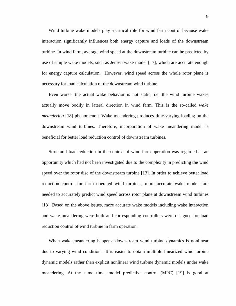
Wind turbine wake models play a critical role for wind farm control because wake
interaction significantly influences both energy capture and loads of the downstream
turbine. In wind farm, average wind speed at the downstream turbine can be predicted by
use of simple wake models, such as Jensen wake model [17], which are accurate enough
for energy capture calculation. However, wind speed across the whole rotor plane is
necessary for load calculation of the downstream wind turbine.
Even worse, the actual wake behavior is not static, i.e. the wind turbine wakes
actually move bodily in lateral direction in wind farm. This is the so-called wake
meandering [18] phenomenon. Wake meandering produces time-varying loading on the
downstream wind turbines. Therefore, incorporation of wake meandering model is
beneficial for better load reduction control of downstream turbines.
Structural load reduction in the context of wind farm operation was regarded as an
opportunity which had not been investigated due to the complexity in predicting the wind
speed over the rotor disc of the downstream turbine [13]. In order to achieve better load
reduction control for farm operated wind turbines, more accurate wake models are
needed to accurately predict wind speed across rotor plane at downstream wind turbines
[13]. Based on the above issues, more accurate wake models including wake interaction
and wake meandering were built and corresponding controllers were designed for load
reduction control of wind turbine in farm operation.
When wake meandering happens, downstream wind turbine dynamics is nonlinear
due to varying wind conditions. It is easier to obtain multiple linearized wind turbine
dynamic models rather than explicit nonlinear wind turbine dynamic models under wake
meandering. At the same time, model predictive control (MPC) [19] is good at
10
systematically dealing with constraints which are important for wind turbine control, such
as limits of blade pitch angle and rate. In this situation, one kind of nonlinear model
predictive control, multi-model predictive control (MMPC) [20], was chosen for loads
reduction control of wind turbines under wake meandering.
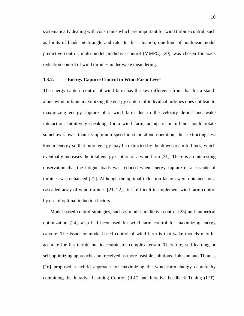
1.3.2. Energy Capture Control in Wind Farm Level
The energy capture control of wind farm has the key difference from that for a stand-
alone wind turbine: maximizing the energy capture of individual turbines does not lead to
maximizing energy capture of a wind farm due to the velocity deficit and wake
interaction. Intuitively speaking, for a wind farm, an upstream turbine should rotate
somehow slower than its optimum speed in stand-alone operation, thus extracting less
kinetic energy so that more energy may be extracted by the downstream turbines, which
eventually increases the total energy capture of a wind farm [21]. There is an interesting
observation that the fatigue loads was reduced when energy capture of a cascade of
turbines was enhanced [21]. Although the optimal induction factors were obtained for a
cascaded array of wind turbines [21, 22], it is difficult to implement wind farm control
by use of optimal induction factors.
Model-based control strategies, such as model predictive control [23] and numerical
optimization [24], also had been used for wind farm control for maximizing energy
capture. The issue for model-based control of wind farm is that wake models may be
accurate for flat terrain but inaccurate for complex terrain. Therefore, self-learning or
self-optimizing approaches are received as more feasible solutions. Johnson and Thomas
[16] proposed a hybrid approach for maximizing the wind farm energy capture by
combining the Iterative Learning Control (ILC) and Iterative Feedback Tuning (IFT).

11
Marden et al. [25] proposed a model-free control strategy by use of game theory and
cooperative control to optimize the axial induction factors to maximize power production
of wind farm.
More recently, one wind farm control strategy had been patented by use of self-
optimizing controller to maximize wind farm power output [22]. Its key idea is: the self-
optimizing controller for an upstream turbine should be configured to control the
upstream turbine in an attempt to maximize the combined total power output of this
upstream turbine and downstream turbines in the wake of this upstream turbine. A better
choice for self-optimizing controller is ESC. In this thesis, the nest-looped extremum
seeking control (NLESC) scheme [22] was investigated for maximizing the wind farm
energy capture.
1.3.3. Summary of Load Reduction and Energy Capture Control of Farm
Operated Turbines
This dissertation study investigates both the load reduction control and energy capture
control in wind farm level. First, the individual pitch control (IPC) is designed for load
reduction to handle the wind variation due to wake interaction via a periodic control
scheme. Then, to deal with the wake meandering phenomenon, a model predictive
control (MPC) scheme is developed for the IPC of the downstream turbine loads. Thirdly,
a novel Nested-Loop Extremum Seeking Control (NLESC) strategy is used to maximize
energy capture of a wind farm.
1.4. Floating Offshore Wind Turbine Control
Both fixed platform and floating platform can be used for offshore wind turbines.
Usually fixed platform is used in shallow water where water depth is usually below 60

12
meters and floating platform is used in deeper water, as shown in Fig. 1.7. Although
Heroneus introduced floating offshore wind turbine in 1972 [26], it was not until 2009
that the first floating wind turbine based on the spar-buoy platform was installed [27].
Fig. 1.7 Status of Offshore Wind Energy Technology [28]
Although fixed offshore wind turbines are easily built based on ripe onshore wind
turbine technology, offshore wind farms in shallow water near the coastline are usually
objected by wildlife groups concerning the effects on avian life along the shores.
Coastline dwellers worry that offshore wind farms block the sea view. Floating wind
turbines are usually installed some distance from the coast such that floating wind
turbines are neither visible nor audible. Sullivan pointed out that “field observations of
offshore wind facilities in the United Kingdom revealed that the facilities may be a major
Source: National Renewable Energy Laboratory

13
focus of visual attention at distances of up to 10 miles” [29]. Extensive deep water areas
exist on the West coast, in Hawaii and the Great Lakes region [30] which are ideal sites
to install floating turbines. From the technical side, the marine and offshore oil industries
have demonstrated ripe technology to build long-term floating structures. Status of
offshore wind energy technology in Fig. 1.7 [28] shows wind resources for deep water
floating turbines (1533GW) is 58% more than the sum of that for transitional depth and
that for shallow water (430GW + 541GW = 971GW).
The wind turbine dynamics has no big difference between onshore turbine and fixed
offshore turbine. However, the dynamics of floating turbine is very different from that of
fixed turbine due to the floating foundation, which brings lots of engineering challenges.
The first question we should ask is how to stabilize floating wind turbine which is a very
interesting and challenging one for control field. A greater challenge for floating wind
turbine is increasing damping in roll motions which are side to side translation in the
plane of rotor rotation [31]. One more problem, negative damping in tower pitch motion
exists for floating offshore wind turbines [32].
Lackner and Rotea [33] proposed tuned mass-spring-damper (TMD) actuator for
stabilization of floating offshore wind turbines. However, mass of TMD 20,00 kg is too
high and TMD stroke (±18 m for active control) is too long, which prevent the practical
applications of TMD. Colwell and Basu [34] proposed a tuned liquid column damper
(TLCD) but the size of TLCD 15.2m was also very long.
In this dissertation study, the problem of interest is to investigate on actuation
schemes of high bandwidth and low-power consumption with light mass and small size.

14
1.5. Problem Statements
Based on the discussion in Sections 1.3 and 1.4, four research problems on wind turbine
control are addressed in this dissertation study as follows.
1) For Region 3 operation, design individual pitch controllers for wind turbine load
reduction with the wake interaction included
2) For Region 3 operation, design model predictive controller for individual pitch
control of wind turbine load reduction with wake meandering considered
3) For Region 2 operation, investigate a novel Nested-Loop Extremum Seeking
Controller to maximize energy capture of a wind farm based on the wind farm
control concept from Seem and Li [22]
4) Investigate the feasibility of an active flow control scheme for stabilization and load
reduction of floating offshore wind turbine based on the floating offshore wind
turbine control concept from Li [35]
1.6. Organization of Thesis
In order to provide appropriate solutions to above four problems, the remainder of this
thesis is organized as follows.
Chapter 2 provides detailed literature review about IPC, wake models, wake
meandering modeling, MPC, wind farm control and control of floating offshore wind
turbines. Periodic control was proposed for IPC of a wind turbine to deal with wake
interaction. MMPC was proposed to deal with wake meandering of wind turbine.
NLESC was proposed to maximize energy capture of a cascade of wind turbines. Vertical
and horizontal vanes are proposed to stabilize floating wind turbines in side-to-side and
fore-aft directions respectively.

15
Chapter 3 presents Jensen wake model, Larsen wake model and simplified wake
meandering model which are used to generate wind profile at downstream wind turbines.
The detailed procedure for implementation is also described.
Chapter 4 presents how to design a periodic controller for wind turbine loads
reduction with the influence of wake interaction. Dynamics simulation of a 600kw 2-
bladed wind turbine was conducted for verification of the proposed DAC controller.
Chapter 5 presents algorithms of multi-model predictive controller and detailed
design for loads reduction of downstream wind turbine under wake meandering.
Dynamics simulation of NREL 5MW wind turbine was conducted for MMPC
verification.
Chapter 6 presents a nested-loop extremum seeking control for maximizing energy
capture of a wind farm. A cascade of 3-turbine were simulated under steady and turbulent
wind for verification of proposed NLESC.
Chapter 7 presents the concept of both vertical and horizontal vane. PI-based
controllers were designed in order to increase damping and alleviate loads of floating
offshore wind turbine in side-to-side and fore-aft directions respectively. Power
assumption of vane actuators was also calculated.
Contributions of this dissertation research are presented in the Chapter 8, along with
suggested future work.

16
Chapter 2. Literature Review
In this chapter, previous research in the subjects relevant to this dissertation research
is reviewed. Understanding of the limitations of the previous research motivates the
research work of this dissertation. First, the work on wind turbine individual pitch control
is reviewed, as well as the periodic control because it is chosen in this study to deal with
the situation of turbine control with wake interaction. As control of farm operated turbine
is a major theme of this dissertation, the state-of-arts wake models and wake meandering
models are reviewed. The objective is to set up the ground for choosing appropriate wake
and wake meandering models for the simulation study of relevant control designs, which
can provide acceptable accuracy of moderate to low computational complexity. Then,
model predictive control (MPC) for wind energy application is reviewed. Finally
reviewed are the floating offshore wind turbine control schemes and wind farm control
strategies for maximizing total energy capture, respectively.
2.1. Review of Individual Pitch Control of Wind Turbine
For Region 3 of wind turbine operation, the expectation is to regulate the power output at
the rated level while reducing the structural load [4]. As turbine size grows larger and
larger, the wind turbine structure tends to be more flexible due to the adoption of lighter
materials and increase in dimension. Load reduction is thus increasingly critical for the
reliability and safety of turbine operation. Improvement in both blade design and control
development can contribute to the alleviation of the fatigue loads for turbine, drive-train
and tower structure. Advanced controller design is considered a relatively cost effective
approach to load reduction, which can compensate for the system and environmental
variations.

17
Load reduction control has been implemented and studied via generator torque
control, blade pitch control and active flow control [36]. For pitch control based load
reduction, both collective pitch control (CPC) and individual pitch control (IPC) have
been studied. For CPC, the pitch angles of all turbine blades are adjusted simultaneously,
and it is appropriate to control the variations slower than one rotor revolution. Due to its
simplicity, CPC has been widely studied and implemented in wind industry [37]. A major
drawback of CPC is the inability of dealing with asymmetric load for actual wind turbine.
Asymmetric load distribution arises most often when the wind speed varies across the
rotor disc due to factors such as vertical wind shear, change in wind direction, yaw error,
and wake interaction [10]. Changes in blade characteristics such as surface icing and
snow accumulation may also lead to asymmetric loading. Such drawback of CPC
becomes a significant limitation nowadays as the turbine diameter becomes increasingly
larger.
In comparison, IPC is achieved by controlling the pitching motion of each blade by
the virtue of separate actuating mechanism [10], with a primary objective of controlling
variations faster than the one rotor revolution. Therefore, IPC aims to deal with
asymmetric loading. Typically the actuators for IPC are required to have higher
bandwidth, for which high-stiffness electric motor actuators are more advantageous.
Various sensing schemes have been investigated, such as strain gage at blade root [10],
local blade inflow [12, 38] and LIDAR [39]. Bossanyi [10] designed LQG-based IPC
controller to alleviate loads at blade roots by use of linear invariant models obtained
through d-q axis. Larsen et al [12] designed gain scheduling PI-based IPC for load
reduction by use of the local inflow angle and relative velocity on each of the blades.

18
Olsen et al. [38] designed IPC based on inflow angle measurements. In particular, Hand
et al. [39] designed an IPC through directly measuring the upwind incoming flow field by
use of LIDAR system, which appears promising for improving the system performance
for feed-forward and model-based feedback control strategies.
Different control design methods have been applied to the IPC development. The IPC
design is in principle a multi-input-multi-output control design problem. For industrial
applications, Bossanyi [37] designed a multi-loop decentralized PI controller where two
separate SISO loops are designed for rotor tilt and yaw moments, respectively. Kanev et
al. [40] proposed an IPC algorithm for rotor balance within pitch and pitch rate
constraints handled by an anti-windup scheme. Jelavic et al. [41] proposed a load
estimation based IPC scheme. Van Engelen [42] proposed a high harmonics control for
wind turbines by use of IPC to reduce loads in high frequency. Specially, a series of field
tests had been conducted at the National Renewable Energy Laboratory (NREL) by
Bossanyi et al. [43-45].
However, the loop coupling is a significant issue, especially among the generator
torque, the first tower fore-aft mode and the first tower side-to-side mode control loops. It
revealed that loop interaction tends to destabilize the closed-loop system when the size of
the wind turbine rotor increases beyond a certain extent [46]. To solve this problem,
centralized control design based on the state-space turbine model has appeared a better
solution. The state-space model based IPC schemes by use of inflow angle measurements
was initially investigated by NREL from 2002 to 2004 [38] and different sensor choices,
such as hot wire, laser Doppler velocimetry system et al, are evaluated for inflow angle
measurements. By far, the optimal and robust control methods have been widely applied

19
to the IPC design, such as the Linear Quadratic Gaussian (LQG) [10] and Η∞ controls
[47]. Besides, Selvam et al. [11] proposed a LQG-based IPC algorithm with feedforward
disturbance rejection by use of the estimation of the wind speed. More recently, IPC was
combined with flap control for load reduction [48].
It is noteworthy that a particular stream of work on wind turbine control has been
developed following Balas’ Disturbance Accommodating Control (DAC) scheme [49].
Several control schemes have been studied following this framework, e.g. Stol [50], Hand
[51], Wright [52], Wright and Fingersh [53], Wright and Stol [46]. Stol [50] applied
Taylor theory to obtain linearized state-space model of wind turbines and applied DAC
for periodic control of a wind turbine. Hand [51] built wind turbine models including
vortex and applied DAC for wind disturbance cancellation along blades. Wright [52]
applied DAC for IPC of a two-bladed turbine. Wright and Fingersh [53] implemented and
tested DAC for IPC of the CART wind turbine in NREL. Wright and Stol [54] applied
DAC for loads reduction at both blades and tower base of wind turbines by use of IPC.
Besides, active yaw control of wind turbine was also achieved through periodic state-
space IPC by Zhao et al. [55]. Recently, Hazim and Stol [56] applied LQR based periodic
control to the IPC for floating offshore wind turbine.
To the author’s best knowledge so far, the reported work on IPC design has included
only the model of vertical wind shear regarding wind asymmetry. For wind farm
operation, the inter-turbine wake interaction is also significant [16]. It is potentially
beneficial for further reduction of dynamic load by including wind turbine wake
interaction.

20
2.2. Wind Turbine Wake Model
For wind turbine operation, wake models have been used to predict wind profiles after an
operating wind turbine [16]. In the past three decades, various wind turbine wake models
have been studied for optimizing wind farm layout, as well as wind turbine load analysis.
These wake models can be roughly categorized into three major classes: numerical
models, kinematic models and field models. In the past three decades, various wind
turbine wake models have been studied for optimizing wind farm layout, as well as wind
turbine load analysis. These wake models can be roughly categorized into three major
classes: numerical models, kinematic models and field models [57].
In numerical wake models, wind turbines are described as distributed roughness
elements, e.g. Templin [58], Newman [59], Crafoord [60] and Moore [61]. Later, these
models were further developed by Bossanyi et al. [62], Frandsen [63], and Emeis and
Frandsen [64]. Although these models are seldom adopted in practice due to the
complexity involved, they can describe the overall wind characteristic for large wind
farms [57]. Kinematic wake models, also known as explicit wake models, are based on
self-similar velocity deficit profiles [57]. The original work of kinematic models for
wind turbine was developed by Lissaman [65], and later modified by Vermeulen et al.
[66]. Jensen [17] and Katic et al. [67] built simple explicit formula to predict wind speed
in the far wake of wind turbines by use of momentum balance, leading to the so-called
Jensen Wake Model. However, linear wake expansion is assumed and initial wake
expansion is neglected in the Jensen Wake Model. Frandsen [68] presented a nonlinear
wake expansion. The kinematic model derived by Larsen et al. [69], known as Larsen
Wake Model, was based on classic wake theory [70]. This model includes the thrust

21
coefficient, the undisturbed wind speed, the rotor diameter, the hub height of wind
turbine and the ambient turbulence intensity. Field models provide the flow information
everywhere in the wake through solving a simplified version of the Reynolds averaged
Navier-Stokes flow equations. The original work on field models was developed by
Sforza et al. [71], and much more work has followed, e.g. Taylor [72], Liu [73] and
Ainslie [74]. A comprehensive coverage of wake models can be found in [57].
Recently Duckworth [75] validated and compared three different wake models by
Ainslie [74], Katic [67] and Larsen [69], respectively. Renkema [76] also validated wake
models by use of testing data in wind farms and wind tunnels. Renkema used second-
order Larsen wake model and pointed out the typo of Larsen wake model in European
Wind Turbine Standards II (EWTSII) [77].
One objective of this study is to integrate appropriate wake models into the process of
plant derivation for controller design. The choice of wake models should be compatible
with both the control-oriented purpose, i.e. capturing the major characteristics of wind
turbine wakes while possessing acceptable simplicity. Numerical and field wake models
are too complex for control design, while the complexity of kinematic wake models
appears appropriate for control design. Therefore, the kinematic wake models are
considered in this study. Furthermore, for wake interaction between turbines in wind farm,
only the far-wake models are needed. Among the available kinematic far-wake models,
the Jensen Wake Model and the Larsen Wake Model have been considered. The Jensen
wake model and the Larsen wake model belong to static wake models. This kind of wake
models is used to predict the average wind speed at downstream wind turbine and
sufficient for wind power prediction and wind farm configuration optimization.

22
Turbulence intensity and ground effect are considered in the Larsen wake model. The
wake diameter in Larsen wake model increases nonlinearly with the distance after
upstream wind turbine. In this situation, the Larsen wake model is more accurate and
chosen in this study.
However, a common limitation of the Jensen and Larsen wake models is that the
wake profile is axisymmetric, while the actual wake profile for the turbines in wind farm
operation is typically asymmetric, e.g. due to wind shear. When controllers of
downstream wind turbines are designed for load reduction, more accurate asymmetric
wake models are needed. For this purpose, an asymmetric wind profile by use of
logarithmic vertical wind shear and Gaussian type wake deficit [78] is chosen to improve
axisymmetric wake models.
In summary, the Larsen wake model and the asymmetric wake model by Van Leuven
[78] are chosen to generate wind profile at downstream wind turbine and for the
controller design in this study.
2.3. Wind Turbine Meandering Wake Modeling
The mechanism of wind turbine wake meandering phenomenon has been investigated
intensively in the past couple of decades. The existing approaches for wake meandering
modeling mainly include Engineering Models [18, 74, 79-83], Computational Fluid
Dynamics (CFD) [84] and Spectral Method [85, 86]. The Engineering Models and CFD
method are time-domain approaches.
The simplest approach to simulating wake meandering is the Engineering Models,
which are built through analytical derivation or analysis of experimental and CFD results.
For Engineering Models, Ainslie [74] considered that the large eddy is the cause of wake
23
meandering and he built the first wake meandering model with the assumption that the
wake meandering effect on wake deficit is proportional to the standard deviation of
turbulent wind directions. While Högström et al. [79] argued that Ainslie’s approach is
incorrect because the standard deviation of wind direction is caused by eddies of all sizes.
Larsen et al. [80] considered that the instability of blade-tip vortex may be one of the
reasons for wake meandering. They simulated wake meandering by use of the analytical
wake model and obtained similar simulation results with the experiment data [81].
Espana [87] proposed that the typical atmospheric length scales may be the reason of
wake meandering but did not suggest any approach to simulating wake meandering. Later,
Larsen et al. [18] (see details on page 381) developed the Pseudo-Lagrangian approach,
which assumes that the wake meandering is a process of releasing a series of wake from
upstream turbines. Thomsen [82] developed the Simplified Wake Meandering Model
(SWMM) which can predict the wake center position at the downstream wind turbine via
the lateral speed at hub-height of the upstream wind turbine. Trujillo [83] developed the
disk-particle model based on the Pseudo-Lagrangian approach.
The most accurate method is via CFD, which however may take very intensive
computational effort to get the wind velocity field within the whole wind turbine wake.
Recently, Jimenez et al. [84] simulated the wind turbine wake meandering by use of
large-eddy simulation (LES), and the oscillating wind direction is used as boundary
conditions.
For simulating turbulent wind, the most common method may be the spectral method
described by Veers [85]. In this method, the spectral model and coherence functions are
used to obtain filtered random variables. Then, filtered signals in spectral domain are

24
converted into real-time turbulent wind by use of Inverse Fast Fourier Transformation
(IFFT). However, Veers [85] did not provide an appropriate coherence function along the
transversal direction for simulating wake meandering. As comparison, Kristensen [88]
provided detailed analysis of lateral coherence which is the critical component of wake
meandering model. Recently, Nielsen [86] also presented an approach to simulating
inhomogeneous, non-stationary and non-Gaussian turbulent wind including wake
meandering, using the coherence model by Davenport [89].
This study aims to use an appropriate wake meandering model which is accurate
enough for wake meandering simulation and yet simple enough for wind turbine
controller design. Compared to the CFD and Spectral Method, the Engineering Models
are simpler approaches that are more suitable for model based controller design. In
Engineering Models, the relatively simpler SWMM [82], as a Pseudo Lagrangian
approach, is considered both incorporating the transversal wake motion and control-
design friendly.
However, SWMM only reflects how the wake is bodily transported along the
transversal direction, but does not include how to generate the wind profile at the
upstream wind turbine. When the transversal wind profile at the upstream wind turbine is
already known, the wake movement at the downstream turbine can be predicted by
SWMM. Often the transversal wind profile at the upstream wind turbine may not be
known, and thus it has to be generated with CFD or the spectral method. Madsen et al.
[90] applied CFD to generate the wind profile at the upstream wind turbine to simulate
wake meandering, but with considerable complexity. In this study, the spectral method is

25
adopted by choosing the Kaimal spectral model [91] and Kristensen’s coherence
functions [88] for the transversal wind at upstream wind turbine.
2.4. Model Predictive Control for Wind Turbine
Model Predictive Control (MPC) predicts the future response of a plant by use of an
explicit model [19] and real-time optimize control inputs with the condition of acceptable
constraints of both control inputs and outputs. In MPC algorithms, a control sequence is
obtained to optimize the future behavior of a plant at every interval, and then the first
input in the optimal control sequence is implemented. MPC has been widely used in
process industries, food processing, automotive, and aerospace [19]. Two characteristics
differentiate MPC from conventional optimal control. One is that the cost function in
MPC is chosen as a finite horizon but in conventional optimal control as an infinite
horizon. The other is that optimization is calculated at every time instant to obtain current
control action in MPC. However, control gain is pre-computed for conventional optimal
control design. The most important advantage of MPC is its capability to deal with hard
constraints of control action and states.
MPC has been a hot topic both within academic and industry during the past three
decades. There have been several excellent textbooks [92-96] to emphasize different
aspects of MPC. An efficient dual mode MPC algorithms and corresponding tuning
techniques were well explained by Rossiter [92]. Generalized predictive control and
implementation issues of MPC were emphasized by Camacho and Bordons [93]. Η2/Η∞
and LMI-based MPC were well summarized by Kwon et al. [94]. Proofs of stability and
robustness, and distributed MPC were emphasized by Rawlings and Mayne [95]. The
MPC theories for hybrid systems are well described by Borrelli et al. [96].

26
For different MPC algorithms, the foremost issue is stability. Stability was not
automatically ensured in early versions of MPC, and not addressed by the proponents of
MPC in process control [97]. However, if plants are stable, stability properties can be
achieved by use of a larger horizon compared with the settling time of plants. Actually,
from 1990s “concern for stability has been a major engine for generating different
formulation of MPC” [97]. Bemporad et al. [98] summarized that stability of MPC can
be ensured through different approaches including terminal constraint [99, 100], infinite
output prediction horizon [101-103], invariant terminal set [104] and contraction
constraint [105, 106], among others. Mayne et al. [97] showed that essential “ingredients”
of different stable MPC schemes include a terminal constraint set, a terminal objective
function, and a local controller.
For wind turbine control applications, Henriksen [107] first applied dual mode MPC
[92] which ensures stability without high computational complexity. Santos [108]
developed damage mitigating control where linear wind turbine models, nonlinear
damage model and nonlinear MPC scheme were used. Kumar and Stol [109] applied the
dual-mode MPC with state-feedback to IPC of wind turbine, and the control input was
obtained through interpolation of those from neighboring controllers based on estimated
velocity at the hub height. Laks et al. [110] designed dual-mode MPC with output
feedback for IPC of wind turbines with preview measurements from the LIDAR sensor.
Soltani et al. [111] designed their wind turbine controller with the LMI (linear matrix
inequality) based Fast MPC in [112] without addressing stability issues. MPC was also
applied to load reduction control via trailing-edge flaps on turbine blades [113], although,

27
the stability issue was not addressed. With consideration of stability and computational
burden, dual mode MPC [92] is deemed a practical approach for wind turbine controls.
However, MPC switching for wind turbines has not been seriously dealt with. Only
Kumar and Stol [114] applied simple interpolation between control inputs from different
controllers for controller switching. More advanced switched MPC algorithms rather than
simple interpolation-based MPC schemes could be used to ensure smooth switching
between MPC controllers. In the initial period of dealing with MPC switching, the
interpolation approach was used for switching [115-117]. During the past decade, several
switched MPC algorithms were built with stability ensured. For example, softly switched
MPC was developed by Wang [118] for application to water supply and distribution
systems. A switched MPC algorithm [119] was also built and applied for steering vehicle
control. The above switched MPC algorithms [118, 119] were developed for piecewise
affine plants, but wind turbine systems impacted by wake meandering do not belong to
piecewise affine plants. Nonlinear model predictive control was also proposed for smooth
switching in [120]. However, tractable nonlinear dynamics for the wind turbine control
under wake meandering is not readily available, which makes the theory difficult to apply.
An LMI based multi-model predictive control (MMPC) algorithm [121] was applied to a
chemical reactor application. In comparison, the MMPC proposed in [122] was
developed without special requirements on state-space models for applications to high
temperature fuel cells [122] and drug infusion control [123].
Besides stability, computational load is a big concern for industrial applications. One
reason why MPC is popular in process control is that the dynamics in process control are
usually very slow (typical time length is several days) which allows enough time to

28
obtain optimized control sequence at every sampling instant. In comparison, for plants
with relatively faster dynamics and high dimensions, such as wind turbine control,
computationally efficient optimization algorithms are needed to implement MPC. In
addition, this study deal with wind turbine control by use of linearized plant models
rather than nonlinear plant models, thus linear MPC methods are considered. In general,
quadratic programming (QP) problems are solved in typical linear MPC algorithms. In
this way, computational efficiency of QP is emphasized below.
The most common methods to solving QP problems include the active set method
(ASM), the interior point method and the Multi Parametric Quadratic Programming
(MPQP) [92]. The ASM is widely used because it provides a systematic way of choosing
a potential active set and iterating through these potential sets to find the global optimum.
Recently more efficient ASM solver was developed for Fast MPC [124]. The interior
point method is becoming more popular than ASM within MPC because converge is
guaranteed in this method and it is faster than ASM. However, the associated
optimization for each iteration requires more computational effort. The toolbox of Fast
MPC by use of the interior point method is also available in [112]. MPQP remains an
active research area for MPC [125, 126]. In MPQP, online optimization computation is
transferred to offline, and all possible control laws are defined offline. In this way, online
QP optimization is converted into set membership tests. However, the potentially large
number of alternative active sets is still an issue [92].
The fastest online MPC solver may be Fast MPC [112] where the interior point
method is used for optimization. However, only open-loop MPC is considered in this tool.
MPQP is a very efficient algorithm for MPC optimization [96]. Moreover, existing MPC

29
algorithms with MPQP are only useful for piecewise affine systems or equivalent systems
[96]. The wind turbine dynamics subject to meandering wake does not belong to the
piecewise affine system because there are no strict partitions for wind turbine states
where wind turbine dynamics can be defined differently when wake meandering exists.
For wake meandering phenomenon, the wake center position on downstream wind
turbine determines wind turbine dynamics rather than wind turbine states. Based on the
above considerations, an active set method [124] is chosen as a QP solver.
In summary, the practical MPC approach, the dual-mode MPC [92], was tested to
deal with wake meandering at first. Then, with the consideration of both characteristic of
wind turbine plants impacted by wake meandering and lower computational burden of
MPC without LMI, the MMPC algorithm [122] was proposed to ensure smooth
controllers switching. An active set optimization solver [127] was chosen for quadratic
programming.
2.5. Dynamic Modeling and Control of Floating Offshore Wind
Turbine
Two main constraints for design of floating offshore wind turbine are stability and cost.
One objective in this study is to invent a new type of floating wind turbine with stability
and cost-effectiveness ensured from the aspect of control.
Driven by potential offshore wind market, during the past decade different floating
platforms have appeared for floating offshore turbines including Barge Platform, Tension
Leg Platform (TLP) [128, 129], Ballast Stabilized Spar Buoy Platform [27, 130] , SWAY
[131] and Dutch Tri-floater [132], as shown in Fig. 2.1 [133]. In particular, the spar-buoy
platform had been used in the first installed floating wind turbine [27]. Butterfield et al.

30
[31] had provided a comprehensive investigation about advantages and disadvantages of
three different floating platforms including Barge, TLP and Ballast (spar). They showed
that TLP should be the most stable platform. Recently, Principle Power proposed a more
practical floating platform, WindFloat [134]. The basic idea follows. The floating turbine
with the WindFloat platform was designed to be assembled onshore and then hauled to
offshore sites by ships in order to avoid high assembling cost on offshore sites due to
undesirable weather and operation difficulties.
Fig. 2.1. Floating Deepwater Platform Concepts: 1) Semisubmersible Dutch Tri-Floater [132] 2) Spar
buoy with two tiers of guy wires [130] 3) Three-arm mono-hull tension-leg platform (TLP)
[128]; 4) Concrete TLP with gravity anchor [129]; 5) SWAY [131]
In order to investigate dynamic behavior of new floating wind turbine concepts, three
main approaches may be used including numerical dynamic modeling, experimental
model-scale testing and full scale prototype testing [135]. From the standing point of both
Source: National Renewable Energy Laboratory

31
research and cost saving, numerical modeling of floating wind turbine are very useful in
the initial period to verify different new concepts of floating wind turbines.
Withee [136] analyzed the coupled dynamics of a floating wind turbine supported on
a floating platform with a tension leg spar buoy [137]. In Withee’s thesis, both nonlinear
wave loads on floating platforms and the aerodynamic loads on wind turbine rotor were
predicted through a coupled way in a stochastic wind and wave environment. The module
to calculate nonlinear wave loading on the floater was integrated into ADAMS [137] and
aerodynamic forces on the floating wind turbine was obtained by use of AeroDyn module
[138]. Finally, both normal operations and extreme wind and wave events were tested to
evaluate the floating platform design. Based on Withee’s work [136], Wayman [139]
optimized parameters of the following platforms: TLP, Tri-Floater platforms, Spar
platforms and Barge platforms. Wayman tested the effects of wind speed, water depth
and viscous damping on these different platforms. Later, Jonkman [28] extended FAST
[140] capability to simulate floating offshore wind turbine through adding the module of
floating platform dynamics including TLP, Barge platforms and Spar buoy platforms.
Recently, Matha [141] compared loads of TLP with that of other platforms for floating
offshore wind turbines. A particular development, the software TimeFloat [142], was
used to analyze the motion and calculate hydrodynamic forces of a special platform
WindFloat [143], for which WAMIT [144] was used as a preprocessor to compute wave
interaction effects. Then, TimeFloat was interfaced with FAST so as to simulate the
coupled dynamics of floating wind turbines and passes data of platform motion back to
TimeFloat [142].

32
Except for FAST [140], Nielsen et al. [145] extended HWAC2 [146] capability to
simulate floating offshore wind turbine through a combination of SIMO/RIFLEX and
HAWC2. SIMO [147] is a time domain software used to simulate multibody systems
which allow nonlinear effects to be included in the wave-frequency range. RIFLEX [148]
is a software of finite element method for static and dynamic analysis of slender marine
structures.
The dynamics of a floating turbine is very different from that of a fixed turbine due to
the floating foundation, which brings many engineering challenges. The top priority is
how to ensure a floating wind turbine’s stability, which is a very interesting and
challenging one for the control field. A greater challenge for floating wind turbine is
increasing damping in the roll motion which is the side-to-side translation in the plane of
rotor rotation [31]. Larsen et al. [32] also claimed that negative damping of tower pitch
motion exists for floating offshore wind turbines and designed PI-based pitch controllers
to ensure the desired bandwidth by use of pole placement, which leads to a stable mode
of floating offshore wind turbines. Although damping of tower motion was successfully
increased, the variations in rotational speed and electrical power are increased 30%.
Jonkman investigated the capability to control floating offshore wind turbine by use
of the PID controller and claimed that the barge-pitch-motion problem was not entirely
resolved through detuning the gains of blade pitch-to-feather controller [149]. Later,
Skaare et al. [150] designed an estimator based blade pitch control to increase the fatigue
life of floating wind turbines.
In addition to PI controllers, modern control methods by use of state-space models
were also investigated to increase tower damping of the floating wind turbine. For

33
example, based on Jonkman’s work [28], Namik and Stol [151] designed periodic control
based IPC for floating offshore wind turbines. Later, Namik and Stol [152] designed
DAC based IPC for offshore floating turbines with both barge platform and TLP. Their
results showed improvement in the regulation of power and rotor speed, as well as
reduction in the tower side-to-side bending moment. However, the tower fore-aft bending
moment is 24% higher than that of the onshore counterpart.
The aforementioned investigations have all utilize the control actuations available on
a typical wind turbine. It is obvious that underactuation is a major issue for floating
offshore wind turbine with the tower/platform stabilization issue present. Furthermore,
tower/platform motion features large inertia, and thus control authority required is
generally siginificant. Therefore, it is necessary to develop effective and feasible
solutions of actuation schemes for stabilizing tower/platform motions.
Lackner and Rotea [33] proposed to use the tuned mass-spring-damper (TMD)
actuator for floating turbine stabilization. This technique has been well received for
building structure control in earthquake engineering. In this work, the TMD actuator is
proposed to reside in the nacelle in order to reduce the fatigue load of the tower-base
bending moment of offshore wind turbine with floating barge-type foundation. Fig. 2.2
shows that variation of tower fore-aft damage equivalent load (DEL) was plotted as a
function of power consumption of active TMD control. It shows that, with about 20%
loads reduction, the power consumption is about 200 kW, which is about 4% of total
wind power production (5MW). Fig. 2.3 shows that the passive TMD system reduced the
tower fore-aft fatigue load by approximately 10%, as compared to a baseline turbine,
while the active TMD control achieved 30% reduction at the expense of about 8% turbine

34
power generated. However, the TMD mass designed is 20,000 kg in order to achieve the
aforementioned performance. This is about 8% of the nacelle mass and 6% of the tower
top mass [153], which requires a dramatic redesign of the nacelle, tower and buoyancy
units. Besides the significant weight addition, another issue is TMD’s large stroke. As
shown in Fig. 2.4, the range of stroke for passive control is approximately ±8 m, while
for active control it is about ±18 m. Because the length of the nacelle is already about 18
m for the wind turbine model considered [153], it is nearly impossible to install TMD in
the nacelle in such a large stroke.
Fig. 2.2 Reduction of Tower Fore-aft Damage Equivalent Load by use of TMD [33]

35
Fig. 2.3 Reduction Percent of Tower Fore-aft Damage Equivalent Load by use of TMD [33]
Fig. 2.4 Comparison of the TMD Stroke for the optimal passive control case and a selected active
control case [33]

36
Except for mass-spring-damper actuation, Colwell and Basu [34] and Luo et al. [154]
designed tuned liquid column damper (TLCD) to stabilize floating offshore wind turbines.
Colwell and Basu [34] claimed loads reductions of up to 55% in the peak response by use
of TLCD under wind and wave excitation but the TLCD was put at tower top with length
of 15.2m, which is too long and brings big troubles for nacelle design. Luo et al. [154]
put TLCD on a turbine’s tower and designed corresponding Η2/Η∞ controllers. However,
wind turbine models were too simple and wind and wave conditions were not clarified
during simulation.
In this study, a new actuator was added [35] to reduce the floating turbine tower
motion and improve stability of a floating turbine. However, tower-top weight should not
be increased too much because higher tower-top weight means higher cost for a floating
offshore wind turbine from the aspects of maintenance and installation. In this situation, a
good choice may be an aerodynamic vane which can take full advantage of aerodynamic
forces and its relative weight is lower compared with the TLCD actuator. Based on the
comments by Butterfield et al., “A greater challenge for floating wind turbine is
increasing damping in roll motions” [31], a vertical vane was used to increase damping of
tower motion in side-side direction. A horizontal vane was also used to avoid negative
damping and increase damping of floating turbines in the fore-aft direction.
2.6. Wind Farm Control
Wind farm control presents control and optimization challenges in order to maximize the
overall power yield or to satisfy the farm level power demand while limiting or
minimizing the structural loading. Although the control strategies for stand-alone turbines
have been widely investigated, e.g. maximizing energy capture [8, 9] and load reduction

37
[10, 155, 156], farm-level wind turbine controls have not been mature enough for
industrial applications. Due to wake interactions between turbines, optimization of
energy capture or load reduction for all the turbines in a wind farm requires globally
optimized operation of individual turbines, i.e. this cannot be achieved by merely
optimizing the operation of individual turbines.
In 1993, Spruce [157] had systematically conducted simulation and control of wind
farms with considering factors including wake interaction, wake transportation delay and
fatigue damage. Due to model reliability issues for complex topology of different wind
farms, Spruce [157] proposed simple ESC algorithm rather than model-based control
method. In his PhD thesis, different cost functions were defined for individual, non-
interacting and interacting turbines in a wind farm in order to maximize financial income
and minimize the turbines’ fatigue damage. Spruce [157] also divided possible wind farm
control algorithms into two different categories: hierarchical control and “multivariable
control”. Hierarchical wind farm control includes plant level control and supervisory
level control. However, all turbine inputs are commanded from a central computer in
“multivariable control”, which should be the same to the concept of centralized control.
Recently various control strategies have been investigated for wind farm controls.
Spudic [23] illustrated the idea of hierarchical wind farm control which is based on the
mixed-integer quadratic programming (MIQP) for load and power optimization by use of
constrained optimal control approach [158] (one type of model predictive control) and the
wind farm simulation platform SimWindFarm [159]. In Spudic’s work, optimal power
reference in a wind farm was obtained for wind farm control and then generator torque

38
and pitch angle of wind turbines were obtained by defaulted controllers when power
references were given.
Soleimanzadeh and Wisniewski [24] conducted wind farm optimization using a wind-
flow based farm model via a 2-D finite volume method. Under the rated wind speed, the
rotor speed at every turbine is dynamically optimized to maximize the total wind energy
capture and the sum of damping factors of wind turbine in both fore-aft and side-to-side
directions based on the wind profiles predicted by the wind flow model. Accordingly,
above the rated wind speed, the pitch angle and power reference at every turbine are
dynamically optimized to meet power demand of a farm while maximizing the sum of the
aforementioned damping factors. Soleimanzadeh and Wisniewski [160] improved
previous work and designed a centralized controller by use of model predictive controller
toolbox and structural loads in low frequency were specially reduced.
Madjidian and Rantzer [161] proposed a stationary turbine interaction model to
calculate the wind speed at downstream turbines by use of wind speed, turbulence
intensity and thrust coefficients at upstream turbines. It showed that the thrust of
downstream turbines can be reduced by decreasing the power production at upstream
turbines while maintaining the power of downstream turbines at the same level.
Brand [162] built a quasi-steady wind farm flow model [163], which relates external
conditions including wind speed, wind direction, turbulence intensity to states including
rotor speed, pitch angle and outputs including power production and mechanical loading
of all turbines. Brand [162] also proposed the inverse mode of the quasi-steady wind
farm flow model, which means that power is input and all other parameters including

39
external conditions and mechanical loads of turbines are output. Then the inverse mode is
used to calculate the distribution of power references over turbines in a wind farm.
Johnson and Thomas [16] proposed a hybrid approach for maximizing the wind farm
energy capture by combining the Iterative Learning Control (ILC) and Iterative Feedback
Tuning (IFT). Both pitch angle and tip speed ratio (TSR) are included as control inputs,
and the simulation model is developed based on the Park wake model [17] for an array of
three turbines.
In 2009, Knudsen et al [164] described the basic idea, approach and preliminary
results for distributed control of large-scale offshore wind farms in the EU-FP7 project
with the objective of wind turbine fatigue loads reduction.
Kristalny and Madjidian [165] proposed a distributed feedforward control scheme for
the possibility of cooperation between turbines and the problem was formulated as a
decentralized model matching optimization.
Madjidian et al. [166] proposed a dynamically distributed power coordination scheme
for fatigue load reduction in wind farms when power demand is below the actual power
production capacity of a wind farm. The control law only required each turbine to
communicate with their neighboring turbines. However, wake model and wind
propagation were not considered in this study. Madjidian et al [167] also extended their
work for reducing structural loads on the turbine tower and the low speed shaft. Recently,
Biegel et al. [168] applied a similar strategy but designed a distributed low-complexity
controller for wind power plant in derated operation for reduction of fatigue loads.
Zhao et al. [169] proposed intelligent agent control for fatigue distribution
optimization of offshore wind farms and the power reference was distributed for

40
balancing structure fatigue loads of individual turbines. In this paper, a wind farm was
modeled as a multi-intelligent agent network.
Horvat et al. [170] showed that power production of a wind farm could be increased
through optimizing rotor speed of individual wind turbines when wind speed is below
rated wind speed. Horvat et al. [170] also showed that the loads at different turbines
could be equalized through optimizing power production references for different turbines
when wind speed is higher than rated wind speed.
Marden et al. [25] suggested a model-free control strategy by use of game theory and
cooperative control to optimize the induction factors to maximize power production of
the wind farm. The Park wake model was used for wind farm simulation. For an array of
three turbines, the resultant axial induction factor for the first upstream turbine was 0.232,
instead of the analytical result of 1/7 in [21].
Bitar and Seiler [171] derived optimal induction factor and total power limit for an
array of turbines by use of dynamic programming. They also pointed out that percentage
of power improvement on greed policy is 8.33% by use of optimal induction factor.
However, in wind field the improvement percentage could be higher than 8.33% because
in wind field the power production maximum for an array of turbines is never reached for
the benchmark of greed policy with inductor factor 1/3 for all turbines.
Park et al. [172] optimized both yaw offset angle and induction factors in order to
maximize wind farm power by use of static game theory. The steepest descent method
was used in this study to calculate optimal yaw offset angles and the induction factors.
41
Guo et al. [173] designed a wind farm controller including an outer loop by use of
model predictive control and an inner loop by use of adaptive control in order to
accurately and smoothly track desired power output reference from a power grid operator.
Most existing studies on wind farm energy capture are model based, except for [16]
and [25]. As the existing wind turbine wake model cannot accurately describe the actual
wake behavior, a (nearly) model-free approach is still considered more appropriate for
wind farm energy capture optimization. Furthermore, since control actuators of wind
turbines only include blade pitch angle and generator torque, it is difficult to implement
control strategies in wind sites when control input blade tip speed ratio [16], rotor speed
[24] or induction factor [25] is used such that in this study generator torque control was
proposed to maximize energy capture of wind farm. In this thesis, a nest-looped
extremum seeking control (NLESC) scheme was presented for maximizing energy
capture of the wind farm [22].

42
Chapter 3. Modeling of Wind Turbine Wake and Wake
Meandering
As mentioned in Chapter 2, wake and wake meandering modeling is critical for
controls of farm operated wind turbines. In this dissertation study, two wake models have
been involved, the Jensen wake model and the Larsen wake model. In this chapter, these
two wake models are described first. Then the logarithmic vertical wind shear model and
Gaussian wake deficit distribution are used to compose the wake profile. Finally a wake
meandering model is presented.
3.1. Jensen Wake Model
The Jensen Wake Model [17] is used to predict the mean wind speed at some distance
behind wind turbines. An upstream and a downstream wind turbine are shown in Fig. 3.1.
The incoming wind speed is V∞, Dr is the diameter of both the upstream and downstream
turbines, and Lhub is the distance between the hub axes of upstream and downstream wind
turbines. Vw is the mean wind speed of the downstream turbine rotor which is located at
the distance xw along the incoming wind direction from the upstream one. The wake
diameter is assumed to grow linearly from Dr at the upstream turbine to Dw at the
downstream turbine, i.e.
2w r wD D kx= + (3.1)
where k is the wake entrainment constant. The mean wind speed at the two turbines are
related via

43
( )2
1 11
1 2 /tw
w r
CVV kx D∞
− −− =
+ (3.2)
where Ct is the thrust coefficient of the upstream turbine.
Fig. 3.1: Illustration of Jensen wake model
3.2. Larsen Wake Model
The Larsen Model [69] considers axisymmetric wake profile with nonlinear growth of the
wake diameter along the distance after the upstream wind turbine. The Larsen wake
model is illustrated in Fig. 3.2, which is a scenario similar to that in Fig. 3.1. In this
illustration, both Cartesian and axisymmetric cylindrical coordinates are used for the ease
of description. The x coordinate is along the prevailing wind direction, with the origin
located at distance x1 before the upstream turbine. The z coordinate is that perpendicular
to the ground surface, with the origin located on the ground. The y coordinate is the other
horizontal direction perpendicular to the x coordinate (i.e. the “lateral” direction), with
the origin located at the hub axis of the upstream turbine. The origin of axisymmetric
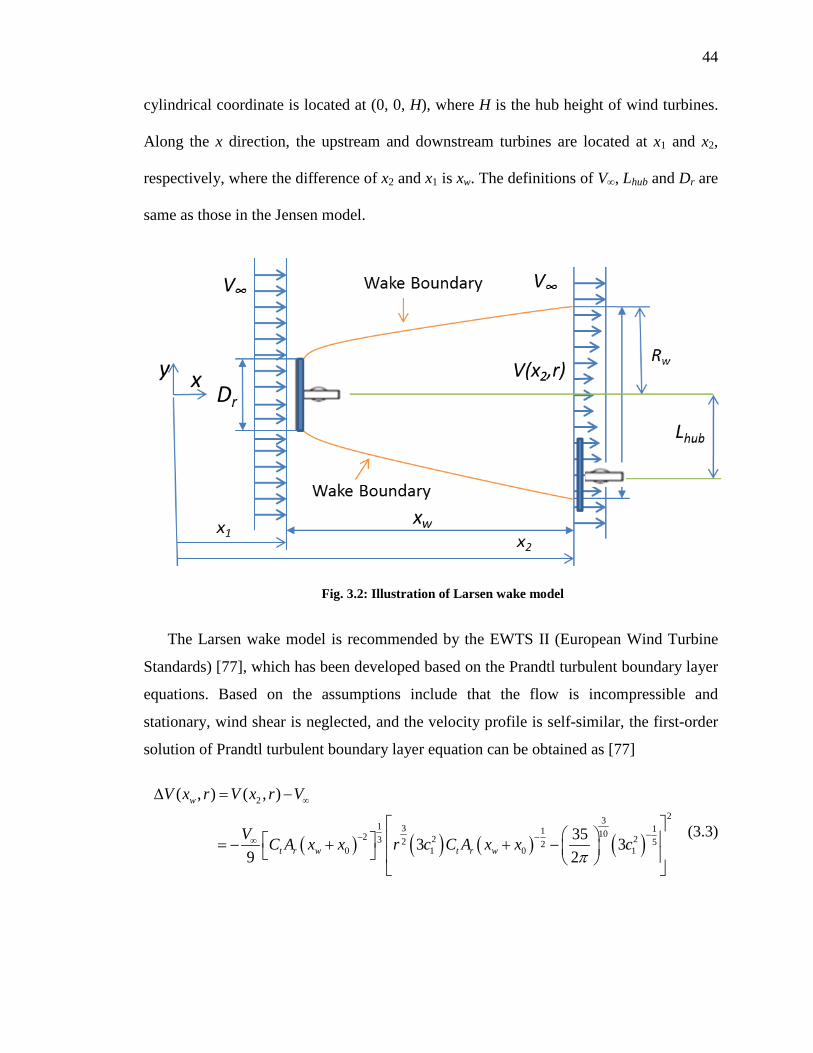
44
cylindrical coordinate is located at (0, 0, H), where H is the hub height of wind turbines.
Along the x direction, the upstream and downstream turbines are located at x1 and x2,
respectively, where the difference of x2 and x1 is xw. The definitions of V∞, Lhub and Dr are
same as those in the Jensen model.
Fig. 3.2: Illustration of Larsen wake model
The Larsen wake model is recommended by the EWTS II (European Wind Turbine
Standards) [77], which has been developed based on the Prandtl turbulent boundary layer
equations. Based on the assumptions include that the flow is incompressible and
stationary, wind shear is neglected, and the velocity profile is self-similar, the first-order
solution of Prandtl turbulent boundary layer equation can be obtained as [77]
( ) ( ) ( ) ( )
2231 3 11 102 2 23 2 52
0 1 0 1
( , ) ( , )
353 39 2π
∞
−− −∞
∆ = −
= − + + −
w
t r w t r w
V x r V x r V
V C A x x r c C A x x c (3.3)

45
where ∆V(xw, r) is the velocity deficit at distance xw from the upstream rotor plane and
radius r from the wake centerline, Ar is the rotor-disc area, Ct is the thrust coefficient, and
the wake radius Rw is
( ) ( ) ( )1
1 15 2 5 31 0
35 32w w t r wR x c C A x xπ
= + (3.4)
The parameters c1 and x0 are given by
(3.5)
(3.6)
where Dr is the rotor diameter. In Eq. (3.6), the effective rotor diameter Deff is given by
(3.7a)
where Ct is again the thrust coefficient of the upstream turbine, and R9.5, the wake radius
at a distance of 9.5 times of the rotor diameter downstream of the turbine, is given by
(3.7b)
where H is the hub height of the upstream wind turbine and Rnb is given by
(3.7c)
where Ia is the ambient turbulence intensity. Although the first-order Larsen wake model
is implemented, the second-order solution could be found in [76]. Besides, at rotor center,
the first-order solution is equivalent to the second-order solution.
( )5 1
52 26
1 0105
2 2eff
t r
Dc C A x
π
−− =
0 3
9.5
9.5
2 1
r
eff
DxR
D
=
−
1 12 1
teff r
t
CD D
C+ −
=−
( )9.5 0.5 min ,nb nbR R H R= +
( )max 1.08 ,1.08 21.7 0.05nb r r r aR D D D I= + −

46
The Larsen Model includes the radial variation of the wind field across the rotor disc,
which is important for load reduction control. Also, the turbulence intensity and ground
effect are included in the Larsen Model. Therefore, the Larsen Model has been chosen in
this study over the Jensen Model for the farm-operated wind turbine control. A common
limitation of the Jensen and Larsen wake models is that the wake profile is axisymmetric,
while the actual wake profile for the turbines in wind farm operation is typically
asymmetric, mainly due to wind shear. To amend for this deficiency, in this study, the
Larsen Wake Model in Eq. (3.3) is used only to calculate the hub-height wind speed
obtained by setting r to zero, while the wind-shear effect and the cross profile of the wake
are included by additional modification described in the following subsections, which can
generate asymmetric wind profile after calculation of hub-height wind speed.
3.3. Wind Shear
In the atmospheric boundary layer, the wind speed increases with height due to the
viscosity of air flow, which is known as the wind shear. Among the wind shear models
developed, the most often considered is the logarithmic vertical wind shear model [174]
(3.8)
where z is the vertical coordinate with the origin located on the ground surface, H is the
hub height, Vhub is the hub-height wind speed, V(z) is the horizontal wind speed along the
z direction, and z0 is the surface roughness which is chosen to be 0.3 (corresponding to
the case of open farm land with few trees and buildings in [174]).
0
0
ln( / )( )ln( / )hub
z zV z VH z
=

47
3.4. Wind Profile of Downstream Turbine Rotor Disc with Wake
Interaction included
For actual wind farm operation, the downstream wind turbine may reside fully or
partially in the wake of the associated upstream turbines. The case of partial wake is more
complicated and bears more impact on the load reduction control of the downstream
turbine. Fig. 3.3 illustrates such a case of wake interaction at the downstream wind
turbine. The smaller disk refers to the rotor of the downstream turbine, while the larger
disk refers to the wake of the upstream turbine developed at the downwind rotor plane.
Fig. 3.3: Illustration of Wake Interaction at the Downstream Turbine
In the rotor disk at the downstream turbine, the wind profile consists of the incoming
wind region and the wake region. In Fig. 3.3, the larger disk refers to the wake region
while the remaining region belongs to incoming wind region. The wind profile in the
incoming wind region is determined via Eq. (3.8), while the hub-height wind speed in the

48
wake region is calculated with the Larsen wake model in Eq. (3.3). However, neither the
Jensen nor the Larsen model includes the vertical asymmetry due to the vertical shear.
Therefore, such models are enhanced in this study to address vertical shear in order to
generate more realistic wind profile in the cross section of the wake.
Existing wind-turbine wake studies [74, 175] have shown that the velocity deficit
profile for axisymmetric wakes can be described by a Gaussian-type function in Cartesian
type of coordinates. In particular, based on the characteristic of Gaussian velocity deficit
distribution, van Leuven [78] proposed the so-called corrected 2-D Gaussian function for
the wind deficit in the cross section of the wake, i.e.
2 2
0
0
ln( / )( , )ln( / )
y z
y z HR R
hubz zV y z V e eH z
−− − ∆ = ∆
(3.9)
where ΔVhub is the hub-height velocity deficit, Ry and Rz are the wake radii in the y and z
directions, respectively. Equation (3.9) indicates an elliptical bell shape for the wake
profile. In this dissertation study, the wake shape is still assumed to be circular, similar to
the Jensen and Larsen wake model.
Then the wake profile at the downstream turbine is given by
(3.10)
where Vwcenter = V(x2, 0, H) is the wind speed at the wake center, following the notations
in Fig. 3.2. As shown in Fig. 3.3, the wind profile in the incoming wind region is
calculated with Eq. (3.8) and that in the wake region with Eq. (3.10). In Eq. (3.10), the
hub-height velocity deficit ∆Vhub=Vwcenter − V∞ is calculated with the Larsen Model (3.3).
2 2
02
0
ln( / )( , , ) ( )ln( / )
w w
y z HR R
wcenterz zV x y z V V V e eH z
−− −
∞ ∞
= − −

49
3.5. Wake Meandering
To facilitate the modeling and control design for more realistic operation of farm turbines,
the wake meandering phenomenon is modeled. Wake meandering is illustrated with the
schematic in Fig. 3.4. The coordinates are defined the same as in Fig. 3.1. Again, the
upstream and downstream turbines are located at x1 and x2, respectively, with spacing xw
= x2 − x1. The incoming wind speed is V∞, and Dw is the wake diameter at the downstream
turbine. The wind profile at the downstream wind turbine can be predicted based on the
incoming wind speed, ambient turbulent intensity, size of wind turbine and relative
position of wind turbines by use of Larsen wake model. The major distinction of wake
meandering modeling is that the wake center moves in transversal direction. The wind
profile at the downstream wind turbine is composed in the following fashion. First, the
transversal speed of the wake at the upstream wind turbine is calculated, then the wake
center at the downstream wind turbine is predicted, finally the wind profile is composed
using the Jensen or Larsen wake model with the wake-center position.
Fig. 3.4: Illustration for Wind Turbine Wake Meandering

50
The procedure for wake meandering simulation is proposed as follows. First, the
spectral method is used to generate wind profile including wake meandering
characteristic at the upstream turbine by choosing appropriate spectral model and
coherence functions, as shown in Fig. 3.5. Second, SWMM (Simplified Wake
Meandering Model) [82] is used to predict the wake motion at the downstream turbine
based on the wind profile at the upstream turbine.
Fig. 3.5: Spectral Method to Generate Turbulent Wind [176]
According to the IEC 61400-1 standard [91], the Kaimal spectrum is given as
( )( )
253
4 /
1 6 /
kk k
k
L US ffL U
σ=+
(3.11)
where Lk is velocity component integral scale parameter, f is the frequency in Hz, k (= 1,
2 and 3) denotes the velocity component, U is the mean wind speed at hub height H,
and σk is the variance determined by the turbulence intensity.
According to the IEC spectral models, the coherence functions of the three wind
velocity components are different. For the v1 component (i.e. the x direction in Fig. 3.4),
the coherence function between points i and j on the grid is defined as [91]
Velocity Spectra
Spatial Coherence
Phase
Random variates
Boundary Conditions
Wind Profile Time Series
Inverse FFTVelocity Spectra
Spatial Coherence
Phases
Frequency
Directly related with wake meandering
White Noise
Low-pass filter
Colored White Noise

51
( ) ( )2 2, 1exp / 0.12 /i j cCoh a fl v l L = − +
(3.12a)
where l is the distance between the two points, a is the coherence decrement, and Lc is a
coherence scale parameter. According to [91], a = 12 and Lc = 5.67⋅min(60, H) m. The
coherence function for the v2 component (i.e. the y direction in Fig. 3.4) is defined as
( ), 2exp /i jCoh cfl v= − (3.12b)
where c = 4.2 [88]. The coherence function for the v3 component (i.e. the z direction in
Fig. 3.4) is defined as
,
10i j
i jCoh
i j=
= ≠ (3.12c)
where w is the velocity in the vertical direction.
Based on Thomsen’s theory [82], the low-pass filtered wind speed in the transversal
direction at the hub height is approximated as the spatially averaged cross-component
wind speed, which is deemed as the wake-center moving speed. Under Taylor’s
hypothesis, the wake-center moving speed for every wake “release” does not change
when the wake transports from upstream wind turbine to downstream wind turbine. Thus,
the wake-center position at the downstream wind turbine is determined by
( )y d filtT V t∆ = ⋅ (3.13a)
( )z d filtT W t∆ = ⋅ (3.13b)
where Vfilt and Wfilt are the filtered velocity along the transversal and vertical direction,
respectively, at the hub center of the upstream wind turbine. The “Wind Profile Time
Series” in Fig. 3.5 are used as input to the low-pass filter. Td is the downstream traveling
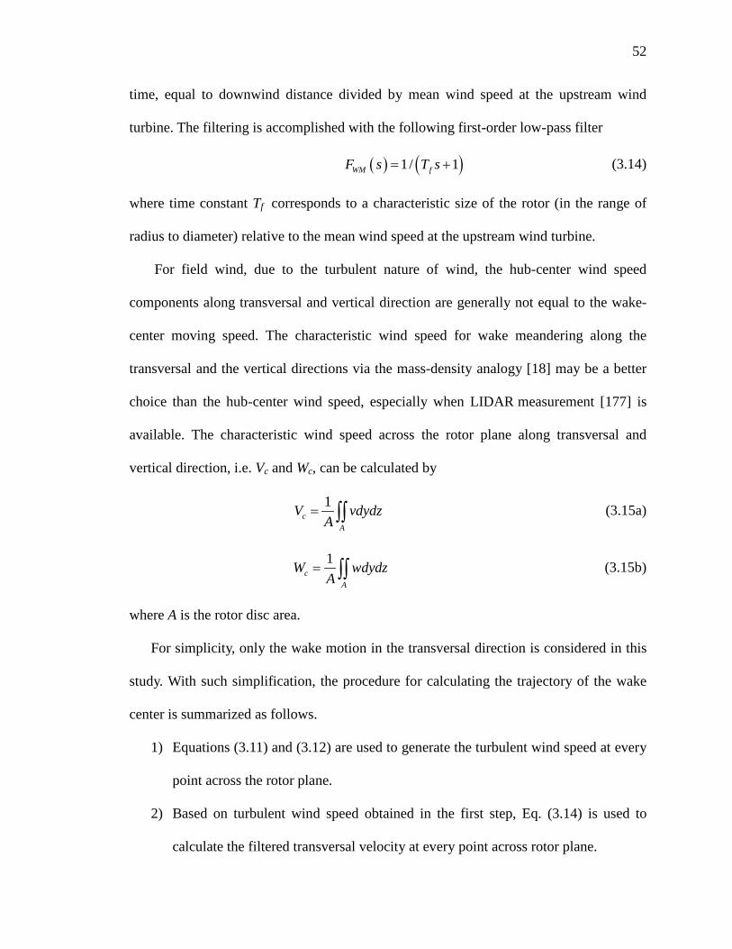
52
time, equal to downwind distance divided by mean wind speed at the upstream wind
turbine. The filtering is accomplished with the following first-order low-pass filter
( ) ( )1/ 1WM fF s T s= + (3.14)
where time constant Tf corresponds to a characteristic size of the rotor (in the range of
radius to diameter) relative to the mean wind speed at the upstream wind turbine.
For field wind, due to the turbulent nature of wind, the hub-center wind speed
components along transversal and vertical direction are generally not equal to the wake-
center moving speed. The characteristic wind speed for wake meandering along the
transversal and the vertical directions via the mass-density analogy [18] may be a better
choice than the hub-center wind speed, especially when LIDAR measurement [177] is
available. The characteristic wind speed across the rotor plane along transversal and
vertical direction, i.e. Vc and Wc, can be calculated by
1c
A
V vdydzA
= ∫∫ (3.15a)
1c
A
W wdydzA
= ∫∫ (3.15b)
where A is the rotor disc area.
For simplicity, only the wake motion in the transversal direction is considered in this
study. With such simplification, the procedure for calculating the trajectory of the wake
center is summarized as follows.
1) Equations (3.11) and (3.12) are used to generate the turbulent wind speed at every
point across the rotor plane.
2) Based on turbulent wind speed obtained in the first step, Eq. (3.14) is used to
calculate the filtered transversal velocity at every point across rotor plane.

53
3) Use Eq. (3.15a) to calculate the wake-center moving speed based on the filtered
wind speed at every point across rotor plane.
4) Equation (3.13a) is used to predict the wake center position based on wake center
moving speed.
When the wake center at downstream wind turbine is known by use of simplified
wake meandering model, the wind profile at downstream wind turbine is composed by
use of the method in Section 4.
3.6. Algorithms for Wake Interaction and Wake Meandering in
TurbSim
TurbSim [176] , a stochastic, full-field, turbulent-wind simulator developed by NREL, is
used to generate wind profile including wake interaction and wake meandering.
Fig. 3.6 Grid Points for Wind Profile in TurbSim [176]
Based on a statistical modeling scheme, TurbSim provides numerical simulation
modeling of 3-D wind speed time series at points in Fig. 3.6. The output of TurbSim can
then be used as input into AeroDyn or other relevant codes like FAST (Fatigue,

54
Aerodynamics, Structures, and Turbulence) [140]. “AeroDyn uses Taylor’s frozen
turbulence hypothesis to obtain the local wind speeds, interpolating the TurbSim-
generated fields in both time and space” [176].
In this dissertation study, the TurbSim is modified to generate wind speed at points in
the 2-D vertical rectangular grids in Fig. 3.6. The wind speeds at these points include
wake interaction and wake meandering characteristics described in the previous sections.
The coordinates adopted in TurbSim is shown in Fig. 3.7.
The procedure for generating wind profiles including wake interaction consist of the
following steps.
1) Calculate wake radius Dw by using Eq. (3.1) or (3.4);
2) For every point (x, y) in Fig. 3.6, determine if it belongs to the wake region or the
incoming wind region. If ( ) ( )2 22( ) / 2hub wx L y H D− + − < , it belongs to the wake
region, otherwise to the incoming region;
3) For every point in the rotor plane: if it belongs to the wake region, the wind speed
at x direction is calculated by Eq. (3.10); otherwise by Eq. (3.8);
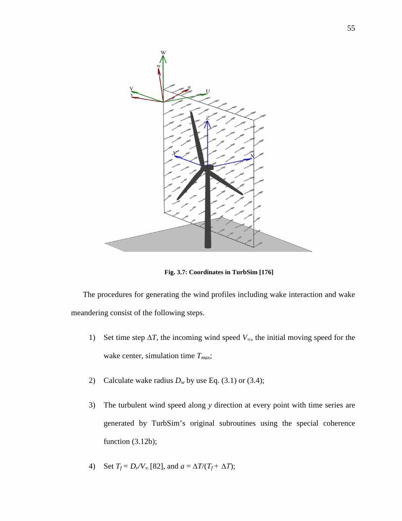
55
Fig. 3.7: Coordinates in TurbSim [176]
The procedures for generating the wind profiles including wake interaction and wake
meandering consist of the following steps.
1) Set time step ∆T, the incoming wind speed V∞, the initial moving speed for the
wake center, simulation time Tmax;
2) Calculate wake radius Dw by use Eq. (3.1) or (3.4);
3) The turbulent wind speed along y direction at every point with time series are
generated by TurbSim’s original subroutines using the special coherence
function (3.12b);
4) Set Tf = Dr/V∞ [82], and a = ∆T/(Tf + ∆T);

56
5) At time t, the turbulent speed along y direction at all grid points across the
rotor plane were added together, and then the sum is divided by the total
number of grid points so as to obtain the average of turbulent speed part Vc (t),
following Eq. (3.15a);
6) For t ≥ ∆T, Vfilt (t) = (1 − a) × Vfilt (t − ∆T) + a × Vc (t) which is derived based
on the low-pass filter Eq. (3.14) as suggested by [178] ;
7) Calculate the wake center position at the downstream wind turbine ∆y(t) by Eq.
(3.13a);
8) t = t + ∆T;
9) If t ≤ Tmax, return to step 5; otherwise, proceed to step 10.
10) Reset t to 0;
11) Define Lhub as the distance between wake center and hub center of downstream
wind turbine and update Lhub based on ∆y(t) and relative position of
downstream and upstream wind turbines;
12) Calculate wake radius Dw by using Eq. (3.1) or (3.4);
13) For every point (x, y) in Fig. 3.6, determine if it belongs to the wake region or
the incoming wind region. If ( ) ( )2 22( ) / 2hub wx L y H D− + − < , it belongs to
the wake region, otherwise to the incoming region;
14) For every point in the rotor plane: if it belongs to the wake region, the wind
speed at x direction is calculated by Eq. (3.10); otherwise by Eq. (3.8);

57
15) t = t + ∆T;
16) If t < Tmax, go to step 11;
Simulated wind profiles along with corresponding controllers could be found in
Chapter 4 and Chapter 5.

58
Chapter 4. Individual Pitch Control of Wind Turbine
Including Wake Interaction
In this chapter, the individual pitch control for load reduction of a downstream wind
turbine is designed based on static wake of upstream turbine. The asymmetric wake
model described in Chapter 3 is adopted to predict the wind profile across the rotor of the
downstream wind turbine without considering the time-varying phenomenon of wake
meandering. According to the composite wind profile within the rotor disc, the LQ
control design is performed for segments along azimuth. In order to obtain more accurate
model for IPC design, an artificial wind pattern, named as equivalent circular wind
profile, is generated. As benchmark, the DAC control scheme is also implemented based
on the vertical wind shear only.
The remainder of this chapter is organized as follows. When wake interaction is
considered, the controller switching strategy adopted is described in the Section 4.1.
Section 4.2 presents how to obtain more accurate linearized state-space models by use of
equivalent circular wind profile and different pitch reference in terms of the azimuth
angle. The DAC and periodic control design are reviewed in Sections 4.3 and 4.4,
respectively. Simulation results are shown in Section 4.5. This part of work is concluded
in Section 4.6.
4.1. Controller Switching Strategy
A relatively general situation of wake interaction is illustrated in Figure 3.3, which is
used for idea-proof simulation study in this chapter. The upstream and downstream

59
turbines are assumed to be at the same height. The wake interaction is mixed with the
vertical wind shear, which makes the case more complicated than what has been dealt
with in the previous DAC design, e.g. by Wright [52, 53]. To deal with this situation, we
have resorted to the periodic control scheme by Stol [179], where the rotor disc is divided
into a number of circular sectors in terms of the azimuth angle, and the LQ controller is
designed for every sector, similar to the illustration in Fig. 4.1. The overall control is
realized by switching between these segmental controllers. Instead of the scheme of
equal-azimuth segmentation of 24 sectors in [179], in this study, we have considered the
change in the H∞ norm of the wind turbine models between individual sectors and then
reduce the number of sectors for controller design.
4.2. Determination of Local Pitch Reference along Azimuth
For IPC, due to the asymmetry nature of the wind across the rotor disc, the reference for
the blade pitch angle varies with the azimuth angle. In this study, as in many other similar
studies on wind turbine controls, NREL’s FAST software [140] is used to obtain the
piecewise linear models. If the linearized state-space models along the azimuth are
obtained by use of “FAST linearization” module [140], the blade pitch angle is the same
for different azimuth angles. Such approximation would result in more inaccuracy when
wake induced asymmetry is included. In order to obtain more accurate linearized state-
space models of wind turbine along the azimuth, it is preferred to obtain the pitch
reference for different azimuthal angles for any specific wind profile.

60
Fig. 4.1 Switching IPC Controller Strategy
As for linearization of the wind turbine model, an operating point is usually defined
by the combination of the blade pitch angle, the rotor speed and the wind speed. The
detailed linearization theory and procedure that is followed are described in detailed in
[52]. Typically, there are two approaches to obtaining linearized state-space models of
wind turbine by use of “FAST linearization” module. One method is that a steady-state
solution is computed to obtain the linearized state-space models, and the other is that an
unsteady solution is computed with the initial condition. For the former method, the pitch
angle and the rotor speed converge to the operating point when the wind profile is
provided. In order to obtain such steady-state solution, the pitch reference is obtained for
a specific azimuth angle with the help from a so-called equivalent circular wind profile

61
(ECWP). For a specific radial profile of wind speed along the blade length at certain
azimuth angle, an ECWP is created by duplicating this profile for all different azimuth
angles, as shown in Fig. 4.2. Such a fictitious wind profile is generated for obtaining
steady-state solution which can help derive the local pitch reference.
Fig. 4.2 Equivalent Circular Wind Profile (ECWP)
When all pitch references are obtained along azimuth by use of ECWP, the
corresponding linearized state-space model along azimuth are obtained by use of
unsteady state solution and original wind profile. In this situation, the initial pitch angle
of different blades should be set as the corresponding pitch reference at the corresponding
azimuth angle, the initial rotor speed should be set as rated rotor speed in Region 3 and
the running time should be less than one period in order to make sure that rotor speed
does not change very much.

62
4.3. Disturbance Accommodating Control
The DAC control design procedure [49] is briefly presented in this section. More details
are available in Wright [52]. The state-space model of wind turbine dynamics can be
described as
dx Ax Bu u= + +Γ (4.1a)
y Cx= (4.1b)
where x is the state vector, u is the control input vector, y is the measurement vector, ud is
the disturbance vector, A is state matrix, B is the input matrix, C relates the measurement
vector with the state vector, and Г is the disturbance gain matrix. A critical step in DAC
design is to model the periodic change of wind load due to vertical wind shear with the
so-called “disturbance generator”, whose dynamics is described with
( ) ( )d du t z tθ= (4.2a)
0( ) ( ); (0)d d d d dz t F z t z z= = (4.2b)
where zd is the state vector for the disturbance generator. For wind shear disturbance
related with 2-blade wind turbine and step wind disturbance,
1 0 00 0 1
θ
=
(4.3a)
2
0 1 00 0
0 0 0dF
= −Ω
(4.3b)
where Ω is the rotor speed.

63
In order to include the disturbance dynamics into the control design, the state vector
is augmented by including the disturbance vector. The feedback control law can be
expressed as
[ ]ˆ ˆˆ ˆ Td d du Gx G z G x z= + = (4.4)
where [ ]DG G G= .
The state observer is designed as
ˆ ˆ ˆ ˆ( ) dx Ax Bu K y y u= + + − +Γ (4.5a)
ˆ ˆy Cx= (4.5b)
The disturbance state estimator is designed as
ˆˆ ˆ( ) ( ) ( )d d dz t Fz t K y y= + − (4.6)
Finally augmented state space model can be expressed as
[ ]ˆ ˆˆ ˆT T
d dx z L x z Ky = + (4.7)
where
d
d
A BG KC BGL
K C Fθ+ − Γ +
= − (4.8a)
[ ]TdK K K= (4.8b)
Then the transfer matrix of the feedback controller can be calculated as
1( ) ( )T s G sI L K−= − (4.9)
The DAC provides an elegant solution to analytically incorporating the vertical shear
into an LTI system framework. However, the disturbance generator is based on a
simplification of the vertical shear, and such simplification may limit its application to
actual wind turbine operation.

64
4.4. Periodic Control
Stol [179] adopted the periodic control strategy to implement DAC. At first, the state-
space models along azimuth were obtained. In this method, the wind shear was not
modeled as the disturbance in the state-space models. Only the hub-height wind
disturbance was chosen. The change of state-space models along azimuth showed the
wind shear characteristics. Then the MIMO controllers were designed based on these
models. Finally, for closed-loop realization, the controllers were switched along azimuth.
Stol [179] divided the rotor disc into 24 segments along azimuth which means each
segment includes 15°. Recently, the LQR and periodic control schemes were used for
IPC of offshore wind turbines without disturbance terms in the state-space model [151].
In this study, the LQR and periodic control methods are used for the segmented plant
models.
The LQR method is simply described in the following, for which the details can be
found in any standard optimal control text. The disturbance term is not considered in the
state-space model. The system described by
x Ax Bu= + (4.10a)
y Cx= (4.10b)
with the cost function defined as
0
( )T TJ x Qx u Ru dt∞
= +∫ (4.11)
For minimizing the above cost, the state feedback control law is
u Gx= (4.12a)
where G is given by

65
1 TG R B P−= − (4.12b)
and P is found by solving the Algebraic Riccati Equation
1 0T TA P PA PBR B P Q−+ − + = (4.13)
The weightings in Q and R matrices need to be adjusted to improve the performance of
the controller.
Similarly, the state observer can be designed
ˆ ˆ ˆ( )x Ax Bu K y y= + + − (4.14a)
Using the feedback control law ˆu Gx= , we have
ˆ ˆx Lx Ky= + (4.14b)
where L A BG KC= + − . Thus, the equivalent transfer function of the closed loop
system is
1( ) ( )T s G sI L K−= − (4.15)
4.5. Simulation Results
4.5.1. Simulation Platform
To evaluate the effectiveness of the proposed IPC scheme, simulation study has been
conducted with FAST [140], Aerodyn [138] and TurbSim [176] developed by NREL,
along with Matlab Simulink. TurbSim is modified to generate wind profiles, as
described in Chapter 3. Wind profile files generated by TurbSim are the input files of
Aerodyn and FAST. Aerodyn is a preprocessor of FAST for calculating the aerodynamic
loads on the turbine blades, which can be used in FAST. FAST can be used to model the
dynamics for both two- and three-blade, horizontal-axis wind turbines. Control
simulation with FAST has been facilitated by the Simulink interface. In this study,

66
TurbSim is modified to generate the wind profile including wake interaction and the
ECWP. Both the upstream and downstream wind turbines used for this study adopt the
model of NREL’s CART (Controls Advanced Research Turbine) facility [180], which is
a two-blade 600 kW variable-speed-variable-pitch turbine.
4.5.2. Wind Profile with Wind Shear and Wake Effect
The allocation of the upstream and downstream turbines is shown in Fig. 3.2. As
mentioned in Chapter 3, the Larsen wake model was chosen. The incoming wind speed
V∞ is assumed to be 18m/s, the ambient turbulence intensity is 18%, the diameter of the
upstream turbine Dr for CART [180] is 46m. For modern wind farms, xw/Dr is usually
designed as 8 to 10. In this study, this ratio is assumed to be 8. Typical values of thrust
coefficient Ct range from 0 to about 1. When the power coefficient reaches its maximum,
thrust coefficient Ct is about 0.728. This study adopts 0.7 for Ct. Application of the
Larsen wake model gives that the diameter of the wake at the downwind turbine grows to
204.22 m, and the wind speed at the wake center becomes 16.76 m/s.
The wind profile was then generated through TurbSim [176] by modifying the
relevant program codes to incorporate the wake related wind velocity superposition.
Usually the typical wind speed consists of the mean and the turbulent components. In
TurbSim, the turbulent portion of wind is generated first following the spectral density
function specified, and then the mean wind speed is added to form the final wind profile.
As a simplified treatment, this study does not consider the turbulent portion of wind. It is
worthwhile to point out that turbulent generally increases in the wake, which implies
increased fatigue load for the downstream turbines.

67
In the TurbSim codes provided by NREL, the rotor disc is regarded as a whole to
calculate the mean wind speed. Since this study includes the wake interaction as well, the
mean wind speed profile across the disc has to be calculated within two areas: the area
without wake effect and that with velocity overlap due to wake effect. The TurbSim
codes have been modified accordingly to generate the wind profile including wake effect.
Figure 4.3 shows the 2D wind speed distribution within the rotor disc of the downwind
turbine due to the wind shear only, while Figure 4.4 shows the profile reflecting the wind
velocity overlap based on the Larsen wake model and the wind shear model with Lhub
equal to 0.9Rw.
4.5.3. ECWP and Different Pitch Reference along Azimuth
Recall in Section 2, the ECWP refers to the scenario that the wind speed along the
azimuth direction is the same but is different along the radial direction (i.e. along the
blade length). For the simulation example, the ECWP is obtained through modifying
TurbSim with the following procedure. The wind information is first extracted at some
azimuth and then copied to all azimuths. For example, if we want to generate an
equivalent circular wind profile at 45° azimuth as shown in Figure 4.4, we need to copy
the wind distribution at 45° azimuth to all azimuths, as shown in Figure 4.5. For different
azimuth angles, the corresponding ECWP needs to be generated respectively to obtain the
corresponding pitch reference. All the pitch references obtained along azimuth for the
special wind profile in Figure 4.4 are plotted in Figure 4.6.

68
Fig. 4.3 Wind Speed Distributions within Rotor Disc due to Wind Shear
Fig. 4.4 Wind Profile with Wind Shear and General Wake Interaction

69
Fig. 4.5 Equivalent Circular Wind Profile for The Simulation Example
Fig. 4.6 Pitch Reference along Azimuth Obtained with ECWP

70
4.5.4. Model Linearization for Individual Pitch Control
The 9-state space models for IPC Design were obtained by use of “FAST linearization”
module, with the descriptions of the states listed in Table 4.1. Three measurement outputs
were used for state estimation: the generator speed, the tip deflection of the first
asymmetric flap mode, i.e. (∆x1−Δx2)/2, and the fore-aft moment on the tower base. The
disturbance inputs include wind shear and hub-height wind disturbances and the averaged
state-space models were used across the rotor plane when DAC approach was used.
When the periodic control and LQR methods were used, our treatment does not include
disturbance input, and the circular wind profile needs to be used to generate the
corresponding state-space models.
Table 4-1: State Description for a 9-state Wind Turbine Model (CART)
4.5.5. Rotor Disc Segmentation
Initially the rotor disc is divided into 24 sectors (similar to Stol [179]), each covering 15°
azimuth angle. Accordingly, 24 state-space models are obtained along the azimuth angle.
As the variation of wind turbine dynamics is considered non-uniform in azimuth angle,
such simple segmentation may be too conservative for some sectors. Therefore, we use
States Description ∆x1 1st tower fore-aft bending moment ∆x2 Drivetrain rotational-flexibility ∆x3 Perturbed blade-1 1st flap deflection ∆x4 Perturbed blade-2 1st flap deflection ∆x5 Derivative of state 1 ∆x6 Perturbed rotor rotational speed ∆x7 Derivative of state 2 ∆x8 Perturbed blade-1 1st flap velocity ∆x9 Perturbed blade-2 1st flap velocity

71
the variation of the H∞ norm of the plants between neighbored sectors to justify the
segmentation scheme. Instead of considering the infinite bandwidth, the difference of
maximum singular value ranging from DC to 100 rad/second between state-space models
of neighboring sectors along azimuth is plotted, showed in Figure 4.7.
The 100 rad/second is considered the 40 dB below the DC magnitude response.
Segmentation along azimuth is based on the following two rules.
1) If the difference in the maximum singular value for neighboring state-space
models is below 4 dB, it is merged into the neighboring segment.
2) The difference in the maximum singular value between neighboring state-space
models should not be greater than 6 dB.
Fig. 4.7 Maximum Singular Value Difference within Rotor Disc

72
Notice that these two rules can be adjusted by controller designer, based on different
robustness need. In other words, if lower robustness is required, the norm difference can
be increased.
Based on these rules, the number of the controllers is reduced from 24 to 16. The
sectors centered at azimuth angle 45°, 75°, 105°, 135°, 225°, 255°, 285° and 315° were
merged to their respective neighbor sectors, as shown in Figure 4.8.
Fig. 4.8 Sixteen Segments of Rotor Disc after Segment Merge
4.5.6. Comparison of Switching and Non-switching Controller
The wake induced wind profile in Figure 3.2 is then used to test the switching control
schemes. The DAC based controller was designed based on the averaged state-space
model obtained under 16.8 m/s hub-height wind speed including wind shear. Sixteen
switching controllers are designed to reduce the load based on state-space models with
different pitch reference along azimuth. Figure 4.9(a) shows the temporal profile of the

73
tower-base fore-aft moment using the switching controller designed based upon the wake
model versus the standard DAC control with only the wind shear considered. The
corresponding spectra in Figure 4.9(b) show that the primary mode at 1 Hz is
significantly suppressed, while some higher harmonics are slightly increased.
a) Steady-state Temporal profile
b) Spectra
Fig. 4.9 Tower-base Fore-aft Bending Moment using the Proposed Method (Switch) and DAC
(No Switch)
0 10 20 30 40 50 601000
1050
1100
1150
1200
1250
Time (Second)
Fore
-Aft
Mom
ent (
kN*m
)
No SwitchSwitch
1 1.5 2 2.5 3 3.5 4
0
10
20
30
40
50
60
70
Frequency (Hz)
Spec
tra of
For
e-aft
mom
ent (k
N*m)
SwitchNo Switch

74
Similar load control performance is demonstrated for the tower-base side-to-side
moment, as shown in Figure 4.10. Significant reduction is observed for 1 Hz while load
increased for higher harmonics (close to 3 Hz and 4 Hz) modes.
a) Steady-state Temporal Profile
b) Spectra
Fig. 4.10 Tower-base Side-to-side Bending Moment using the Proposed Method (Switch) and
DAC (No Switch)
0 10 20 30 40 50
150
160
170
180
190
200
Time (Second)
Side
-Sid
e M
omen
t (kN
*m)
No SwitchSwitch
1 1.5 2 2.5 3 3.5 4
0
2
4
6
8
10
12
14
16
18
Frequency (Hz)
Spec
tra o
f Sid
e-si
de M
omen
t (kN
*m)
SwitchNo Switch

75
Figure 4.11 shows that the mean and variation of rotor speed were both reduced
regarding the rated speed of 41.7 rpm, by use of the switching controllers compared with
the traditional DAC. Therefore, the proposed strategy can indeed improve load reduction
and speed regulation for turbines subject to wake interaction.
a) Steady-state Temporal Profile
b) Spectra
Fig. 4.11 Rotor Speed using the Proposed Method (switch) and DAC (no switch)
0 10 20 30 40 50 6041.7
41.75
41.8
41.85
Time (Second)
Rot
or S
peed
(rpm
)
No SwitchSwitch
1 1.5 2 2.5 3
0
0.005
0.01
0.015
0.02
0.025
0.03
0.035
Frequency (Hz)
Spec
tra o
f Rot
or S
peed
(RPM
)
SwitchNo Switch
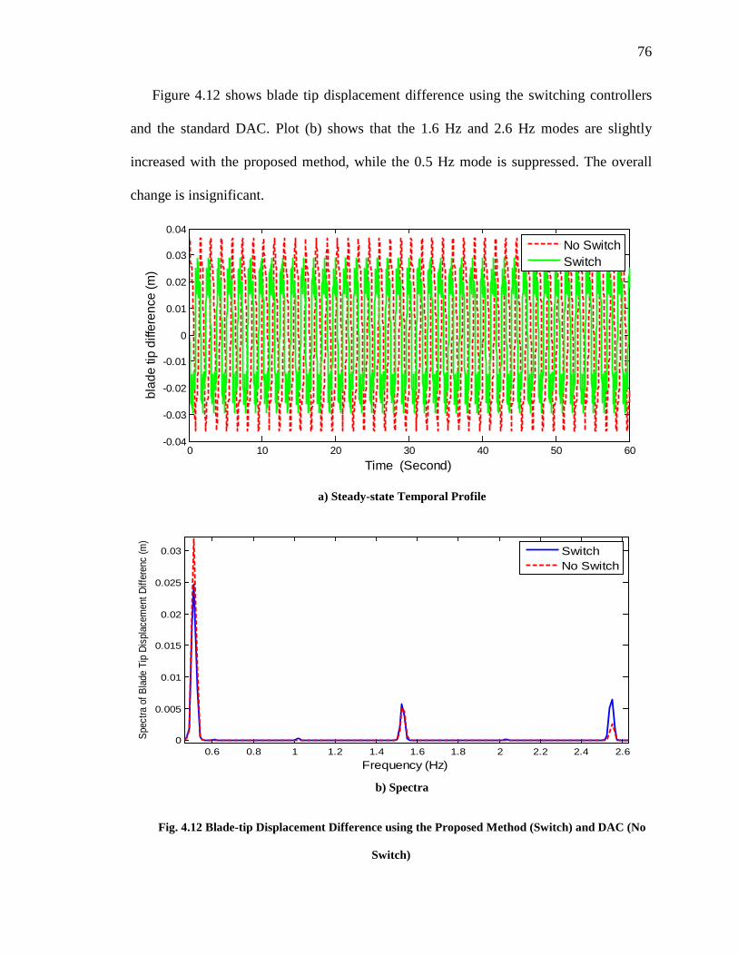
76
Figure 4.12 shows blade tip displacement difference using the switching controllers
and the standard DAC. Plot (b) shows that the 1.6 Hz and 2.6 Hz modes are slightly
increased with the proposed method, while the 0.5 Hz mode is suppressed. The overall
change is insignificant.
a) Steady-state Temporal Profile
b) Spectra
Fig. 4.12 Blade-tip Displacement Difference using the Proposed Method (Switch) and DAC (No
Switch)
0 10 20 30 40 50 60-0.04
-0.03
-0.02
-0.01
0
0.01
0.02
0.03
0.04
Time (Second)
blad
e tip
diff
eren
ce (m
)
No SwitchSwitch
0.6 0.8 1 1.2 1.4 1.6 1.8 2 2.2 2.4 2.60
0.005
0.01
0.015
0.02
0.025
0.03
Frequency (Hz)
Spec
tra o
f Bla
de T
ip D
ispl
acem
ent D
iffer
enc
(m)
SwitchNo Switch

77
4.6. Summary
This chapter presents an improvement on the IPC scheme for load reduction by including
the wake interaction. The Larsen wake model is applied for composing the rotor wind
profile for downstream turbines under wake interaction, and a switched control strategy is
thus developed based on the composite wind profile. The wind profile was generated by
modifying the TurbSim codes. The idea of equivalent circular wind profile was proposed
to obtain different pitch references along azimuth. When different pitch references along
azimuth are used, more accurate state-space models of wind turbine can thus be generated
via FAST linearization. Based on such models, the IPC are designed following both the
DAC and the periodic control frameworks. Simulation results showed that the tower-base
fore-aft bending moment, the tower-base side-to-side bending moment, the rotor speed
fluctuation and the blade-tip displacement difference are significantly suppressed.

78
Chapter 5. Model Predictive Control of Wind Turbine
Including Wake Meandering
As described in Chapter 1, the meandering phenomenon of upstream turbine leads to
time-varying nature of wind loads on the downstream turbines. This implies additional
time-varying asymmetry of the effective turbine model. Therefore, the wind turbine load
reduction control is further complicated. To deal with such odd, a practical solution is to
design (model predictive) controllers based on a number of linearized wind turbine
models under the predicted patterns of superposed wind profile. Then, a relevant issue
arises: – how to handle the “intermediate region” between any two selected patterns.
Instead of using the controller interpolation idea, this dissertation study adopts a
Multiple-Model Predictive Control framework, which is built upon a consecutive process
of plant updating via the recursive Bayesian estimation. In other words, the plant for each
step of controller (MPC) design is obtained from weighting a number of pre-defined plant
models.
Section 5.1 describes multi-blade coordinate (MBC) transformation which is used to
convert the azimuth-periodic wind turbine models/variables into a time-invariant
counterpart under static wind profile. A practical approach with enhanced stability
robustness and relatively low computational burden, the Dual Mode MPC, is described in
Section 5.2. The multiple-model predictive control algorithm is presented in Section 5.3.
Finally, simulation study is given in Section 5.4, which validates the effectiveness of the
proposed control strategies.

79
5.1. Multi-Blade Coordinate Transformation
Typical multi-body analysis of wind turbine dynamics is built upon several sets of
coordinates: the earth coordinates, the blade coordinates (Fig. 5.1), the coordinates on the
nacelle (Fig. 5.2) and the coordinates on the tower base (Fig. 5.3) [140].
Fig. 5.1 Blade Coordinate System [140]
Fig. 5.2 Nacelle Coordinate System [140]

80
Fig. 5.3 Tower-base Coordinate System [140]
The Blade Coordinates in Fig. 5.1 rotate with wind turbine blades. Under this set of
coordinates, the wind turbine dynamics is periodic in azimuth under steady wind, as well
as the corresponding state-space models. As consequence, the dynamic loads of wind
turbine (e.g. blades and tower) are periodic. Such temporal/spatial change of plant model
presents significant difficulty for controller design. Considering the maturity and
convenience of controller design in linear time-invariant (LTI) models, the Multi-blade
Coordinate (MBC) transformation has been developed to convert the time/azimuth
periodic plant models/variables into their time-invariant counterparts [181, 182]. The
MBC transformation is a widely used technique in the helicopter field [183]. In the
remainder of this section, the MBC transformation is reviewed by following the
description by Bir [2].

81
According to MBC, for a 3-blade turbine, three nonrotating degrees of freedom
(DOF), joq , j
cq and jsq , can be converted into three rotating DOF’s, 1
jq , 2jq and 3
jq , by
the following transformation:
1
2
3
j jo
j jc
j js
q qq T qq q
=
(5.1)
where jbq is the jth rotating DOF for the bth blade with b = 1, 2, 3. In the non-rotating
frame, joq , j
cq , jsq are the average mode, the cosine-cyclic mode and the sine-cyclic
mode, respectively. The transformation matrix T and its inverse are defined as
1 1
2 2
3 3
1 cos sin1 cos sin1 cos sin
ψ ψψ ψψ ψ
=
T (5.2)
11 2 3
1 2 3
1 1 11 2cos 2cos 2cos3
2sin 2sin 2sinψ ψ ψψ ψ ψ
−
=
T (5.3)
where ψ1 , ψ2 and ψ3 are azimuthal angles of blades 1, 2 and 3, respectively. It is trivial to
justify that ψ1 + ψ2 + ψ3 = 2π at any time. Notice that the inverse of matrix T is needed in
order to convert a rotating DOF to its nonrotating counterpart, while the nonsingularity of
T is guaranteed by the geometrical relationship amongψ1, ψ2 and ψ3.
Based on Eqs. (5.1), (5.2) and (5.3), the wind turbine dynamics of the 3-blade
horizontal-axis wind turbine can be converted from the rotating frame to the non-rotating
frame as follows, based on the procedure developed by Bir [181]. In general, the
aeroelastic analysis of wind turbine dynamics deals with lumped-element equations of
motion (EOM) and its output equations in the following form:

82
+ + = + dMX CX KX Fu F w (5.4)
= + + +v d dY C X C X Du D w (5.5)
where X is the coordinate vector, u is the control input vector, and w is the disturbance
vector. M denotes the mass matrix that contains direct blade inertias and blade-tower
coupling inertias, C contains both structural damping and gyroscopic terms, and K
contains structural and aerodynamic stiffness terms as well as the centrifugal effect. F
and Fd denote the control input, and disturbance input matrices, respectively. Y is the
output vector. Cv and Cd are output matrices for velocity and displacement, respectively.
D and Dd are the feedthrough matrices for the control input and the disturbance input,
respectively.
For wind turbine control problem, the motion vector is defined as
1 1 11 2 3 1 2 3 1 2 3 =
TT j j j m m mFX X q q q q q q q q q (5.6)
where XF is an nF×1 column vector representing the nF fixed-frame-referenced DOF, jbq
is the jth rotating DOF for the bth blade, and m is the total number of rotating DOFs for
each blade. The length of vector X is nF + 3m.
As the aeroelastic codes (for example, FAST) generate equations of motion in a
numerical form, the substitutional method is typically used to convert the EOM (5.3) into
the non-rotating form [181]. Based on Eq. (5.1), vector X in the rotating-frame is related
to its counterpart in the nonrotating-frame vector, XNR, via the foregoing MBC
transformation,
1 NRX T X= (5.7)
where

83
1
( 3 ) ( 3 )
×
+ × +
=
nF nF
nF m nF m
IT
T T
T
(5.8)
and
1 1 1 = TT j j j m m m
NR F o c s o c s o c sX X q q q q q q q q q (5.9)
By combining the coordinate variables and their velocities into vector z, i.e.
=
Xz
X (5.10)
EOM (5.4) and (5.5) can be rewritten in the state-space form, i.e.
dz Az Bu B w= + + (5.11)
dY Cz Du D w= + + (5.12)
where A, B and Bd are the state matrix, input matrix, and disturbance matrix, respectively.
Then, Eq. (5.11) and (5.12) can be transformed to the nonrotating frame as
= + +NR NR NR NR NR dNRz A z B u B w (5.13)
= + +NR NR NR NR NR dNRY C z D u D w (5.14)
where
1211
213 2 22 11
00020NR
TTTA A
T T TT TT
−
−
Ω = − Ω +Ω ΩΩ (5.15)
11
111
00NR c
TB BT
T
−
−
=
(5.16)
1c NRu T u= (5.17)

84
11
11
00dNR d
TB B
T
−
−
=
(5.18)
[ ]110 1 1 2 2 2 1NRC T C T C T C T−= +Ω (5.19)
[ ]1 2C C C= (5.20)
110 1NR CD T DT−= (5.21)
110dNR dD T D−= (5.22)
2
2 2
2 ( 3 ) ( 3 )
0 ×
+ × +
=
nF nF
nF m nF m
tT t
t
(5.23)
1 1
2 2 2
3 3
0 sin cos0 sin cos0 sin cos
tψ ψψ ψψ ψ
− = − −
(5.24)
3
3 3
3 ( 3 ) ( 3 )
0 ×
+ × +
=
nF nF
nF m nF m
tT t
t
(5.25)
1 1
3 2 2
3 3
0 cos sin0 cos sin0 cos sin
tψ ψψ ψψ ψ
− − = − − − −
(5.26)
( ) ( )
1
3 3
uF uF
uF uR uF uR
n n
c
n n n n
I
TT T
T
×
+ × +
=
(5.27)

85
( )
10
3 ( 3 )
FoxFo
Fo mo X Fo mo
IT
T T
T+ +
=
(5.28)
In the above equations, nuF and nuR are the number of control inputs in the fixed and
rotating frames, respectively; Fo and mo are the number of outputs in the fixed and
rotating frames, respectively. More details on MBC transformation for 3-blade wind
turbine are available in [181].
When time-invariant models Eqs. (5.13) and (5.14) are used for controller design,
measurements at rotating frame, such as the blade-root flapwise moment, need to be
converted into the non-rotating frame by use of the inverse of matrix T, and then
corresponding variables at fixed frame are used for controller design with MBC.
Similarly, the control inputs (pitch angles) in the fixed frame need to be converted back
to the rotating frame again by use of matrix T. See the controller configure when MBC is
used in Fig. 5.4.
Fig. 5.4 Multi-Blade Coordinates for Controller Design
5.2. Dual-Mode Model Predictive Control
The terminology dual mode control is originally from nonlinear control [5]. This control
strategy covers two modes: one mode is used when the system is far from the operating
Controller
Wind Turbine Simulator
T-1
Measurements at fixed frame
Measurements at Rotating FrameGenerator Torque
Pitch Angle at Fixed Frame
Pitch Angle at Rotating Frame
T

86
point; the other mode is used when the system is close to the operating point. Then, the
control strategy automatically switches into different modes when the system is operating
at different desired states.
In MPC, the “dual mode” notation is different from that in nonlinear control. The
Dual Mode in MPC indicates how the predictions are set up. The main motivation of dual
mode prediction is to handle the predictions over an infinite horizon which implies
nominal stability [92]. Usually, the first mode refers to the period within the prediction
horizon, i.e. the estimation of k i kx + where i =0, 1, 2, …, Hp−1; while the second mode is
the state prediction beyond the prediction horizon, i.e the estimation of k i kx + for i = Hp,
Hp+1,… . The controller for the first mode is designed by use of classical MPC
algorithms. The controller for the second mode is designed by use of special algorithms,
such as LQR, for ensuring stability. The Closed-loop Paradigm (CLP) is considered as a
good framework for dual-mode MPC [92]. In this study, the CLP MPC by Rossiter [92]
is adopted, which is simply described in the following.
The discrete-time state-space model of the given plant is
1
1
k k k
k k
x Ax Buy Cx
+
+
= +=
(5.29)
The control input has the following dual-mode form

87
1| 1
| 1
|
|
c c
c
y c
c
k k
k k k
k n k k nCLP
k n k
n nk n k
Kx cKx c
Kx cuKx
K x
+ +
+ + −
+
−+
− + − + − += − − Φ
(5.30)
and matrix Φ is the closed-loop state matrix with the use of state feedback gain K
Φ = −A BK (5.31)
The cost function for CLP is defined as
2T Tc cxJ c S c c S x= + (5.32)
where
1 1c
T T Tk k k nc c c c+ + − = (5.33)
2 2( ) ( )T T Tc c c cu cu c cS H diag Q H H diag R H H PH= + + (5.34)
2 2( ) ( )T T Tcx c cl cu clu c clS H diag Q P H diag R P H PP= + + (5.35)
2
KK
P K
− − Φ = − Φ
(5.36)
0 00
cu
BKB B
HK B KB B
− = − Φ −
(5.37)
The detailed derivation could be found in the Chapter 7 in the book [92].
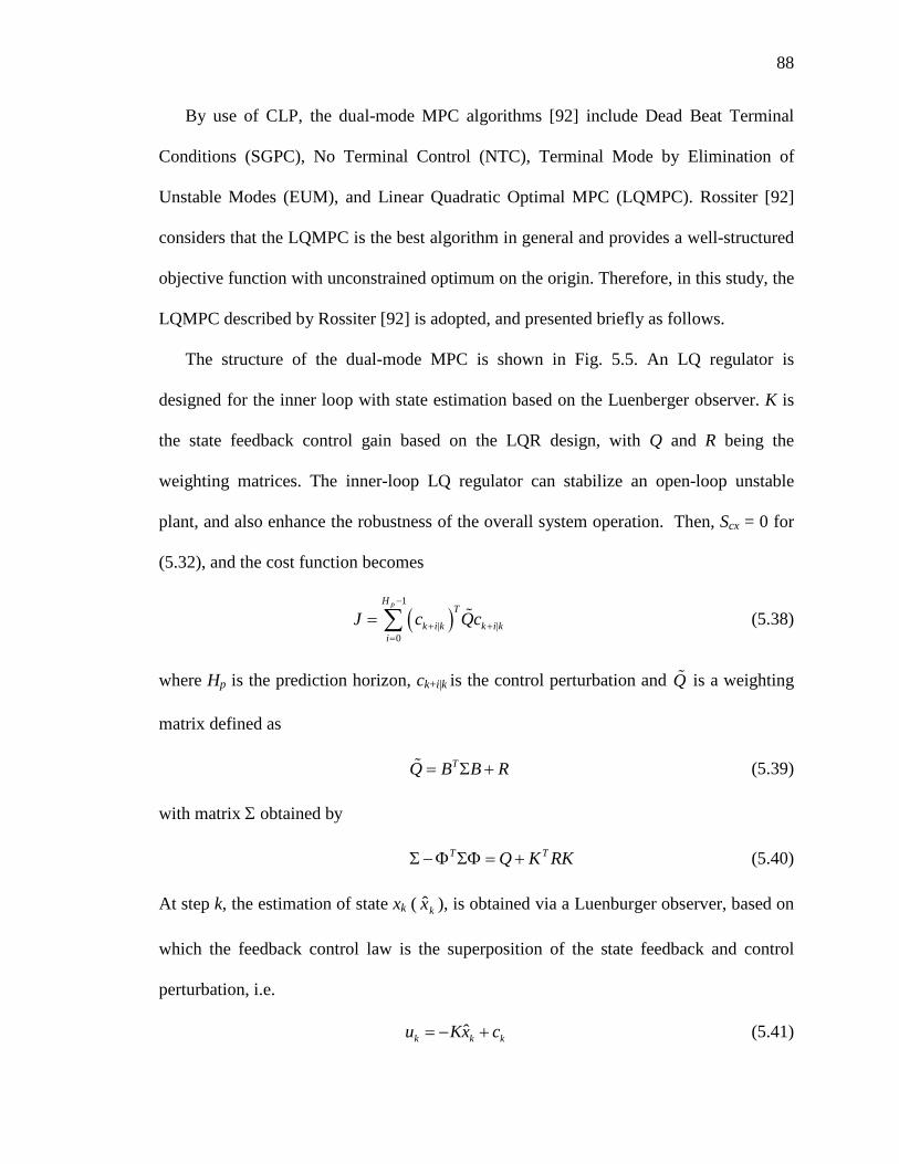
88
By use of CLP, the dual-mode MPC algorithms [92] include Dead Beat Terminal
Conditions (SGPC), No Terminal Control (NTC), Terminal Mode by Elimination of
Unstable Modes (EUM), and Linear Quadratic Optimal MPC (LQMPC). Rossiter [92]
considers that the LQMPC is the best algorithm in general and provides a well-structured
objective function with unconstrained optimum on the origin. Therefore, in this study, the
LQMPC described by Rossiter [92] is adopted, and presented briefly as follows.
The structure of the dual-mode MPC is shown in Fig. 5.5. An LQ regulator is
designed for the inner loop with state estimation based on the Luenberger observer. K is
the state feedback control gain based on the LQR design, with Q and R being the
weighting matrices. The inner-loop LQ regulator can stabilize an open-loop unstable
plant, and also enhance the robustness of the overall system operation. Then, Scx = 0 for
(5.32), and the cost function becomes
( )1
| |0
pHT
k i k k i ki
J c Qc−
+ +=
= ∑ (5.38)
where Hp is the prediction horizon, ck+i|k is the control perturbation and Q is a weighting
matrix defined as
= Σ + TQ B B R (5.39)
with matrix Σ obtained by
Σ −Φ ΣΦ = +T TQ K RK (5.40)
At step k, the estimation of state xk ( ˆkx ), is obtained via a Luenburger observer, based on
which the feedback control law is the superposition of the state feedback and control
perturbation, i.e.
ˆk k ku Kx c= − + (5.41)

89
where ck is the control perturbation based on the MPC to be designed.
Fig. 5.5. Block Diagram of Dual-mode MPC based IPC control
The constraints for the control input are formulated as
0kMu N− ≤ (5.42)
where
2
0 00
k k k
K IK KB I
u x cK K B KB I
− − Φ − = + − Φ − Φ −
(5.43)
k clu k cu ku P x H c= + (5.44)
1 1p
T
k k k k Hu u u u+ + − = (5.45)
1 1p
T
k k k k Hc c c c+ + − = (5.46)
Eq. (5.44) is a compact form of Eq. (5.43) which is derived from Eqs. (5.29) and (5.41).
Substituting Eq. (5.44) into (5.42), the constraints for the control perturbation becomes
cu k clu kMH c N MP x≤ − (5.47)
When the observer is used, constraints condition is
ˆcu k clu kMH c N MP x≤ − (5.48)
-K
Optimizer
Wind Turbine Simulator
Luenberger Observer
Bending Moments at Blade Roots
States
+
MPC Controller
Ck
Pitch Actuator Generator Speed
T-1
T

90
The control perturbation ck is calculated by solving the quadratic programming problem
associated with cost function (5.38) under inequality (5.48). In the beginning, the author
attempted to use the Matlab function quadprog in order to solve the quadratic
programming optimization problem, but quadprog could not handle the number of
constraints involved in this problem. Finally the qpOASES solver [127] was used as it
performed better for the large-dimension optimization problem involved.
The foregoing scenario is for the dual-mode MPC design based on a single state-
space model of wind turbine. However, when the wake center moves, the aerodynamic
loads on the downstream wind turbine will change, which in turn changes the wind
turbine dynamics significantly. A practical solution to such situation is to obtain
linearized state-space model for different wake-center positions, based on which the MPC
controller can be designed. This can be illustrated in Fig. 5.6, the solid horizontal line
stands for wake center range which is equally divided by n points for controller switching.
For the n points, based on the corresponding wake-center positions, different steady wind
profiles without wake meandering but including wake interaction are generated in order
to obtain the linearized state-space models. As shown in Fig. 5.7, the IPC controllers are
switched based on wake center position, and each controller is designed with the
aforementioned dual-mode MPC controller design procedure.

91
Fig. 5.6. Illustration for Wake Center Positions for Controller Switching
Fig. 5.7 Controller Switching for Dual-mode MPC based IPC Control under Wake Meandering
5.3. Multiple-Model Predictive Control
In previous section, the dual-model MPC controllers were simply switched to deal with
wake meandering. In order to deal with time-varying operating conditions due to wake
meandering and ensure smooth controller transition, a multiple-model predictive control
(MMPC) algorithm [20, 122, 184] is used in this section.
The concept of MMPC design is shown in Fig. 5.8. Assume the system behavior can
be approximated as some weighted average of the N linear discrete-time state-space
Wind Turbine Simulator
MPC Controller 1
measurementsPitch Actuator
MPC Controller 2…
MPC Controller n
Switching
Wake Center Position
Generator Speed
Pitch Input
Rated Power ÷Generator SpeedGenerator Torque

92
models
| 1 1 1− − −= + i i i ik k k kx A x Bu (5.49)
| |=i i ik k k ky C x (5.50)
where i = 1, …, N is the model index and 1ku − is the control input perturbation.
Fig. 5.8 Algorithm for Multiple-Model Predictive Control
This study follows the framework in [8], but in a simplified fashion, with the random
noise and plant perturbation ignored. With such simplification, state estimation is based
on the Luenberger observer, i.e.
| | 1 | 1ˆ ˆ ˆ( )i i i i ik k k k k k kx x L y C x− −= + − (5.51)
The weighting for different models are calculated by use of Bayesian probability
1
0
µ
µ=
> =
≤
∑
iik
kNji
kkj
ik
p ppw
p
(5.52)
Plant
State Estimation 1
State Estimation 2…
State Estimation n
Weighting Calculation
Set PointOptimization
Prediction
Constrained MPC
uk yk

93
where μ is an artificial limit on the probability, and is effectively the threshold for
determining the set of “active” models. Recursively, the probability of the system
behavior belonging to the i-th model is
( )( )
1
11
exp 0.5
exp 0.5
i T i ik k ki
k ns T s s
k k ks
pp
p
ε ε
ε ε
−
−=
− Λ=
− Λ∑ (5.53)
where
| |ˆ ˆi i i ik k k k k k ky y y C xε = − = − (5.54)
Λ is a diagonal scaling matrix for the residuals and determined based on the covariance of
each model. Λ needs to be tuned for plant performance adjustment.
The cost function in terms of the incremental control is defined as
( ) 12
T Tf U U H U g U∆ = ∆ ∆ + ∆ (5.55)
where
[ ]1 1T
k k k mU u u u+ + −∆ = ∆ ∆ ∆ (5.56)
( )2 2Ta a
u c e y c eH W S S W S S= + (5.57)
( ) ( )02Ta a a
c e y sp x cg S S W Y S S U= − − − (5.58)
2
1
( ) ( )
ˆ
y x
i i
i iNa i ix k k
ii i p
p n n
C AC A
S w x
C A=
× ×
=
∑
(5.59)
( )
( ) ( ) ( ) (( 1) )
0u u
u u u uu u
n n
e
n n n n p n m n
I
SI I
×
× × × × − ×
=
(5.60)

94
( )1 1
( )
0
y u
i iN
a ic k
i i i p i i i
p n p n
C BS w
C A B C B= −
× × ×
=
∑
(5.61)
nu is the number of control inputs, ny is the number of measurements, p is the prediction
horizon for the states, m is the control horizon.
For wind turbine IPC, the control inputs need to first observe to the following range
constraints:
( ) ( ) ( )
( ) ( ) ( )
min max
min
max
0 /180 0 /180 0 /180
90 /180 90 /180 90 /180
k j
Tr r r
Tr r r
u u u
u u u u
u u u u
π π π
π π π
+< <
= − − −
= − − −
(5.62)
where ur is the pitch reference in degree while the unit of uk+j is radian. In this study, pitch
references were obtained through the FAST linearization module [140] when rated rotor
speed and wind profiles were known. Also, the constraints for pitch rate (radian/sec) are
1min max
+ + −−< <k j k j
s
u uu u
T (5.63)
where Ts is the sampling period, and
[ ]min 10 /180 10 /180 10 /180π π π= − − − Tu (5.64)
[ ]max 10 /180 10 /180 10 /180π π π= Tu (5.65)
As the MMPC design is applied to the time-invariant models in the non-rotating
frame, the constraints (5.62) in the rotating frame need to be converted into the non-
rotating frame via the MBC transformation Eq. (5.3). Besides, the cost function is valued
with the incremental control input rather than control input. The MMPC for wind turbine
control incorporating MBC transformation is shown in Fig. 5.9.

95
Fig. 5.9 Illustration of MMPC based Wind Turbine Control Incorporating MBC Transformation
The (blade pitch) control input sequence in the rotating frame is denoted as
(5.66)
and its counterpart in the non-rotating frame is denoted as
(5.67)
By use of MBC transformation, we have
(5.68)
The relationship between blade pitch control input and its increment is
(5.69)
where

96
[ ] ( )
3 3 3 3
3 3 3 3
3 3 3 3 1u u
x x
x x
x x n m n m
I II I
M
I I× × × +
− − = −
(5.70)
Assuming that matrix P is the pseudo inverse of the matrix M in Eq. (5.70), we have:
1k
k
uP U
u−
= ∆
(5.71)
Based on Eqs. (5.62), (5.68) and (5.71), the range constraints of blade-pitch increment
in the rotating frame can be expressed as
( ) ( ) ( ) ( )
maxmin
maxmin
maxmin 1 11 1 1 1× + × × + + × × + × ×
< ∆ <
u uu un m n mm n m n
uu Tuu T
P U
uu T
(5.72)
Similarly, rate constraints on blade pitch in the fixed frame can be expressed as
( ) ( ) ( ) ( )
maxmin
maxmin
maxmin
maxmin 1 1 1 1u u u u
s RF s
m n n m n m m n
uu Tuu T
T T P U T uu T
uu T× × × + × × + × ×
< ∆ <
(5.73)
( ) ( )( )1
1 0 0 1 0 00 1 0 0 1 00 0 1 0 0 1 00 0 0 1 0 0 1 0
0 0 1 0 0 1u u
RF
m n m n
T
× × + ×
− − −
= −
−
(5.74)

97
Finally, the quadratic programming problem is to minimize cost function Eq. (5.55)
with constraints Eqs. (5.72) and (5.73), and it is solved again by qpOASES [127].
5.4. Simulation Study
5.4.1. Simulation Platform
To evaluate the effectiveness of the foregoing two MPC schemes, similar to Chapter 4,
simulation study has been conducted with the NREL 5MW Wind Turbine Model [185]
using the FAST [186], Aerodyn [138] and TurbSim [176] software packages and
Matlab Simulink.
A particular effort in this study is that the author modified the TurbSim codes from
NREL in order to generate the wind profile including wake interaction and wake
meandering. The NREL 5MW [185] onshore turbine model is used, which is a three-
blade variable-speed variable-pitch turbine, with rotor diameter of 126 m, blade length of
61.5 m and hub height of 87.6 m.
5.4.2. Simulated Wake Meandering Model
Allocation of upstream and downstream turbines follows Fig. 5.10. Both turbines are
assumed to be the NREL 5MW turbine, as described in Appendix B. The distance
between upstream and downstream wind turbines are 8Dr. The incoming wind speed V∞
is assumed to be 18 m/s, and the ambient turbulence intensity is 18%. Based on the
spectral method and simplified wake meandering implemented in TurbSim, the wake-
center trajectory along the transversal direction at the downstream wind turbine is
obtained as shown in Fig. 5.11, which shows that the wake-center position falls within
the range of [−144, 173] m in the transversal direction and the coordinate of the averaged

98
wake center position is −14.5 m. The wake-center moving speed in the transversal
direction falls within the range of [−2.5, 3.0] m/s. Based on the Larsen wake model, the
wake diameter at the downwind turbine grows to 281 m, the mean wind speed across the
wake plane becomes 16.7 m/s and the time constant Tf is 7 for wake meandering in this
simulation case.
Fig. 5.10 Illustration of wake meandering for two turbines in a wind farm

99
Fig. 5.11. Wake Center Trajectory at the Downstream Wind Turbine
The range is divided by 11 nodal points in equal distance. Based on the wake-center
positions corresponding to the 11 nodal points, steady wind profile is generated without
considering wake meandering but including wake interaction and used to obtain
linearized state-space models. When the wake center position is known, Eq. (3.10) is
used to compose the wind profile including wake interaction. Fig. 5.12 shows wind
profiles for two positions of the wake center: one is located at the left most position and
the other is when the rotor center is near the wake boundary. The difference in the wind
profile is clearly observed.

100
(a) Wake center at WC-1
(b) Wake center at WC-11
Fig. 5.12 Wind Profiles at the Downstream Wind Turbine for Different Wake-Center Positions
Horizontal Direction
Verti
cal D
irect
ion
10 20 30 40 50 60
10
20
30
40
50
60
13
14
15
16
17
18
m/ sRotor Disk
Wake Boundary
Horizontal Direction
Verti
cal D
irect
ion
10 20 30 40 50 60
10
20
30
40
50
60
13.5
14
14.5
15
15.5
16
16.5
17
17.5
18
18.5
m/ sRotor Disk
Wake Boundary

101
5.4.3. Model Linearization and MBC Transformation
For each section in Fig. 5.6, the wind profile is assumed steady, and the corresponding
linearized state-space turbine model was obtained from FAST. As shown in Table 5.1, a
9-state dynamic model is considered for the dual-mode MPC, in which the state vector
includes the rotor speed, the shaft rotational strain and the flapwise bending moment for
each blade. For MMPC, a 7-state model is considered by neglecting the drivetrain
rotational-flexibility and its derivative in Table 5.1. The measurements for dual mode
MPC include the generator speed and the flapwise bending moment at the root of each
blade (Table 5.2).
For the illustrative example, and for each wind profile considered, the rotor disc is
divided into 36 sectors, each covering 10° azimuth angle. Accordingly, 36 state-space
models are obtained along the azimuth angle for each wind profile. The MBC [181] is
used to convert the state-space models in the rotating frame to those in the fixed frame.
Then the average system of the 36 linearized state space models in the fixed frame is
obtained by averaging the according A, B, C, D matrices [181].
Table 5-1: STATE DESCRIPTION FOR A 9-STATE WIND TURBINE MODEL (NREL 5MW TURBINE)
Symbol States Δx1 Perturbed Drivetrain Rotational-flexibility Δx2 Perturbed 1st Flapwise Bending Mode of Blade 1 Δx3 Perturbed 1st Flapwise Bending Mode of Blade 2 Δx4 Perturbed 1st Flapwise Bending Mode of Blade 3 Δx5 Perturbed Rotor Rotational Speed Δx6 Derivative of State Δx1 Δx7 Derivative of State Δx2 Δx8 Derivative of State Δx3 Δx9 Derivative of State Δx4

102
Table 5-2: MEASUREMENTS FOR NREL 5MW
Symbol Measurements y1 Generator Speed or Rotor Speed y2 Flapwise Bending Moment at the Root of Blade 1 y3 Flapwise Bending Moment at the Root of Blade 2 y4 Flapwise Bending Moment at the Root of Blade 3
5.4.4. Simulation Results for Dual-Mode MPC Based IPC
The wind profile including wake meandering is then used to test the switching control
schemes. Based on averaged state-space model generated by use of steady wind profile
with averaged wake center position, the baseline MPC controller is designed first. Then,
eleven switching controllers are designed to reduce the load based on state-space models
generated by use of different steady wind profile with different wake center position at
downstream wind turbine. The sampling period is 0.1 seconds and the prediction horizon
is 20. Fig. 5.13(a) shows the temporal profile of the rotor speed using the switching
controller designed based upon wake meandering model and single MPC controller. The
rated rotor speed for NREL 5MW is 12.1 rpm. The corresponding spectra in Fig. 5.13(b)
show that the rotor-speed fluctuation below 0.025 Hz is significantly suppressed.
Fig. 5.14 (a) shows the temporal profiles of the flapwise bending moment at the root
of Blade #1 before and after the wake meandering is considered during controller design.
The corresponding spectra in Fig. 5.14 (b) show that the mode at frequency about 0.13
Hz is suppressed significantly. The flapwise bending moments at other blade roots are
similarly suppressed by 39% at the 1P frequency.

103
a) Steady-state Temporal Profile
b) Spectra
Fig. 5.13. MPC Controlled Rotor Speed with and without Considering Wake
Meandering
0 50 100 150 200 25011.5
12
12.5
13
13.5
14
14.5
15
15.5
Time (Second)
Rot
or S
peed
(rpm
)
Including Wake MeanderingWithout Wake Meandering
0.02 0.04 0.06 0.08 0.1 0.12 0.14 0.16 0.18 0.20
0.05
0.1
0.15
0.2
0.25
0.3
Frequency (Hz)
Spec
tra o
f Rot
or S
peed
(RPM
)
Including Wake MeanderingWithout Wake Meandering
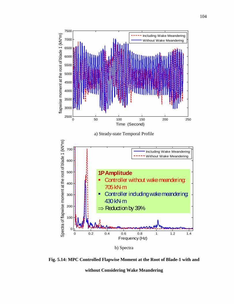
104
a) Steady-state Temporal Profile
b) Spectra
Fig. 5.14: MPC Controlled Flapwise Moment at the Root of Blade-1 with and
without Considering Wake Meandering
0 50 100 150 200 2502500
3000
3500
4000
4500
5000
5500
6000
6500
7000
7500
Time (Second)
flapw
ise
mom
ent a
t the
root
of b
lade
1 (k
N*m
)
Including Wake MeanderingWithout Wake Meandering
0 0.2 0.4 0.6 0.8 1 1.2 1.40
100
200
300
400
500
600
700
Frequency (Hz)Spec
tra o
f fla
pwis
e m
omen
t at t
he ro
ot o
f bla
de 1
(kN
*m)
Including Wake MeanderingWithout Wake Meandering
1P Amplitude Controller without wake meandering:
705 kN⋅m Controller including wake meandering:
430 kN⋅m⇒ Reduction by 39%

105
5.4.5. Simulation Results for MMPC Based IPC
The MMPC scheme is simulated with the scenario of the previous subsection. When
model number N = 1, and the corresponding weighting is 1 in Eqs. (5.59) and (5.61),
MMPC is simplified to single MPC as the baseline controller. Then, MMPC controllers
are designed to reduce the load based on state-space models generated by use of different
steady wind profile with different wake center position at the downstream wind turbine.
The sampling period for MPC design is 0.1 second and the prediction horizon is 20.
The following weighting matrix Λ is chosen for Eq. (5.53):
6
6
6
6
0 0 00 0 00 0 0
1010
10100 0 0
−
−
−
−
Λ =
(5.75)
The weighting matrices with prediction horizon of 20 steps are
7
3
3
3
7
3
3
380 80
1.56 104.69 10
4.69 104.69 10
1.56 104.69 10
4.69 104.69 10
yW
×
× × ×
× =
× × × ×
(5.76)
7
7
60 60
8.2 10
8.2 10uW
×
× = ×
(5.77)
Fig. 5.15(a) shows the temporal profile of the rotor speed using the MMPC designed

106
based upon wake meandering model and single MPC controller. The corresponding
spectra in plot (b) show that the amplitude below 0.03 Hz is significantly suppressed.
a) Steady-state temporal profile
b) Spectra
Fig. 5.15. Rotor Speed with and without Considering Wake Meandering.
Fig. 5.16 (a) shows the temporal profile of flapwise bending moment at the root of
0 20 40 60 80 100 120 14010.5
11
11.5
12
12.5
13
13.5
14
14.5
Time (Second)
Rot
or S
peed
(rpm
)
Including Wake MeanderingWithout Wake Meandering
0.02 0.04 0.06 0.08 0.1 0.12 0.14 0.16
0
0.2
0.4
0.6
0.8
1
Frequency (Hz)
Spec
tra o
f Rot
or S
peed
(RPM
)
Including Wake MeanderingWithout Wake Meandering

107
Blade #1 before and after the wake meandering is considered during controller design.
The corresponding spectra in plot (b) show that the mode at frequency near 0.2 Hz is
significantly suppressed. The flapwise bending moments at other blade roots are
suppressed similarly.
a) Steady-state temporal profile
b) Spectra
Fig. 5.16. Flapwise Bending Moment at the Root of Blade-1.
0 20 40 60 80 100 120 1402000
3000
4000
5000
6000
7000
8000
Time (Second)
flapw
ise m
omen
t at th
e ro
ot o
f bla
de 1
(kN*
m)
Including Wake MeanderingWithout Wake Meandering
0 0.2 0.4 0.6 0.8 1 1.20
50
100
150
200
250
300
350
400
450
500
Frequency (Hz)
Spec
tra o
f flap
wise
mom
ent a
t bla
de 1
root
(kN*
m)
Including Wake MeanderingWithout Wake Meandering

108
Fig. 5.17 shows that the rate constraints of blade pitching are basically satisfied. Fig.
5.18 shows that pitch angle remains within 0° to 90°. Fig. 5.19 shows the weighting
profile between two models at a given instant, where model mode number i means that
models i and i+1 are being used.
Fig. 5.17: Temporal Profile for the Pitch Angle Rate for the MMPC IPC
0 20 40 60 80 100 120 140 160-10
-8
-6
-4
-2
0
2
4
6
8
10
Time (Second)
Pitc
h Ra
te ( °
/s)
MMPCUpLimitDownLimit

109
Fig. 5.18: Temporal Profile of Pitch Angle for the MMPC IPC
Fig. 5.19: Weighting and Model Mode in MMPC
100 105 110 115 120 125 13011
12
13
14
15
16
17
Time (Second)
Pitc
h An
gle
( °)
Pitch Angle 1Pitch Angle 2Pitch Angle 3
0 20 40 60 80 100 120 1400
0.5
1
Time (Second)
Wei
ghtin
g
0 20 40 60 80 100 120 1400
5
10
Time (Second)
Mod
el M
ode

110
5.5. Summary
This chapter presents two MPC based IPC schemes for load reduction of wind turbine
under a wake meandering scenario, i.e. the dual-mode MPC and the MMPC. After
obtaining the linearized state-space models via MBC, switched dual mode MPC are used
to deal with wake meandering and MMPC are designed in order to ensure smooth
controller transition. Compared to the baseline dual-mode MPC with single state-space
model, the variations in the rotor speed and the blade-root flapwise moment are
significantly suppressed by use of switched dual-mode MPC. While compared to the
baseline MPC controller, the variations in the rotor speed and the blade-root flapwise
moment are significantly suppressed by use of MMPC that incorporates wake
meandering in its design.

111
Chapter 6. Maximizing Wind Energy Capture via Nested-loop
Extremum Seeking Control
This Chapter proposes a novel control approach for optimizing wind farm energy
capture with the scheme of nested-loop extremum seeking control (NLESC). Similar to
Bellman’s Principle of Optimality, it has been shown in earlier work that, for cascaded
wind turbines, the axial induction factors of individual wind turbines can be optimized
from downstream to upstream units in a sequential manner, i.e. the turbine operation can
be optimized based on the power of the immediate turbine and its downstream units. In
this study, this scheme is illustrated for wind turbine array with variable-speed turbines
for which torque gain is controlled to vary axial induction factors.
The proposed NLESC scheme is demonstrated with a 3-turbine wind turbine array
using the SimWindFarm simulation platform. Simulation results under smooth and
turbulent winds show the effectiveness of the proposed scheme. Analysis shows that the
optimal torque gain of each turbine in a cascade of turbines is invariant with wind speed
if the wind direction does not change, which is supported by simulation results for
smooth wind inputs. As changes of upstream turbine operation affects the downstream
turbines with significant delays due to wind propagation, a cross-covariance based delay
estimate is proposed as adaptive phase compensation between the dither and
demodulation signals.
The remainder of this chapter is organized as follows. Section 6.1 presents the idea of
nested optimization of cascade wind turbine array based on which the NLESC wind farm
control strategy [22] is proposed. The NLESC framework for wind farm control is
described in Section 6.2. For the extremum seeking control involved, an adaptive phased

112
compensation scheme is also presented to handle the significant delay between upstream
turbine control and downstream power measurement. The simulation study is presented
in Section 6.3, with conclusion in Section 6.4.
6.1. Nested Optimization of Cascaded Wind Turbine Array
For cascaded wind turbine array, the relationships on optimal axial induction factors have
been recently studied by Corten and Schaak [21] based on the 1-D simplified wind
turbine model. Based on this result, the NLESC has recently been proposed in a patent by
Seem and Li [22]. Justification of nested-loop optimization for maximizing energy
capture of a cascade of wind turbines is provided by Dr. Yaoyu Li in Appendix A. Based
on the work [22] and Appendix A, the NLESC for maximizing energy capture of a
cascade of wind turbines is proposed in this section. In this study, the dither extremum
seeking control is adopted as the core of the NLESC although other ESC schemes may
work as well. The key idea of NLESC is: the ESC (or any other appropriate self-
optimizing controller) for an upstream turbine should be designed to maximize the
combined total power output of this upstream turbine and downstream turbines in the
wake of this upstream turbine. A better choice for self-optimizing controller is ESC.
A special case of a wind farm is that there are a cascade of turbines and wind speed
blows from turbine 1 to turbine n. Turbine i+1 to n are in the wake of turbine i, which is
shown in Fig. 6.1. This figure also shows supervisory control loop of turbines. The
control objective is to maximize the total power of turbine i to n through control of
turbine i. The measurement for turbine i is the sum of power of turbines i through n. The
control input is generator torque. In Fig. 6.1, Pi is power of turbine i, ki is generator
torque gain for turbine i, ωi is generator speed of turbine i.

113
Fig. 6.1 NLESC Control for A Cascaded Array of Wind Turbines
6.2. NLESC Based Wind Farm Control Design
Extremum seeking control is used to online search an optimal input uopt(t) which leads to
the maximum or minimum of a generally unknown time-varying cost function l(t, u),
where u(t) ∈Rm is the input vector
( ) arg min ( , )mopt
uu t l t u
∈ℜ= (6.1)
A typical ESC structure to minimum seeking [187] is shown in Fig. 6.2. y(t) is the
measurement of the cost function l(t, u), n(t) is the noise, FI(s) is the input dynamics, FO(s)
is the output dynamics, d1 is the demodulating signal, and d2 is the dither signal;
[ ]1 1( ) sin( )...sin( )Tmd t t tω ω= (6.2)
[ ]2 1 1 1( ) sin( )... sin( )Tm m md t a t a tω α ω α= + + (6.3)
where ωi are the dithering frequencies for each input channel and αi are phase difference
between the dithering and demodulating signals. The dither signal d2 is used to generate
control input perturbation which leads to cost function variance. Then High Pass Filter
k1
Wind1
2 n-1 nMax(P1+P2…+Pn)
Max(P2+P3…+Pn)
Max(Pn)Max(Pn-1+Pn)
ESC 1
kn
2nω
𝜏𝑛
PnPn-1
Pn
kn-1
21nω −
𝜏𝑛−1
Pn-1+Pn
P2
P3+P4…+Pn
k2
22ω
𝜏2
P2+P3…+Pn
P1
21ω
𝜏1
ESC 2 ESC n-1 ESC n

114
FHP(s) is used to remove the DC value of cost function. The demodulation signals d1
works with Low Pass Filter FLP(s) together to extract the signal proportional to the
gradient ∂l/∂u. The integral is used to ensure the stability of controller. The compensator
K(s) is used to accelerate the convergence.
Fig. 6.2 Block Diagram of Dither ESC Algorithms
In the field of wind turbine control, ESC has been studied for maximizing energy
capture of individual wind turbines [8, 188-190]. Creaby et al. [8] proposed multivariable
ESC based on the measurement of the rotor power. Munteanu et al. [188] proposed wind
turbulence as search disturbance instead of sinusoidal search signals for ESC design to
reach maximum wind power. Pan et al. [189] proposed sliding mode ESC for energy
capture improvement of wind turbines. Hawkins et al. [190] used Lyaponov-based ESC
to increase energy capture of wind turbines. The ESC design in this study follows the
guidelines in [187].
In the following, it will be shown how to properly choose output measurement of
ESC to maximize energy capture of wind farm in steady wind and turbulent wind. A
wind farm with three turbines is used as an illustrative example. Turbines 2 and 3 are in
the wake of turbine 1, while turbine 3 is in the wake of turbine 2.
FLP(s)
FHP(s)
−μ/s K(s)
FI(s)l(t,u)FO(s)
d1 d2
n(t)
y(t) u(t)

115
6.2.1. Steady Wind
The generator torque gains are used as designed control input of ESC for both steady and
turbulent wind. The sum of mechanical power of all turbines in the wake of a turbine is
selected as the output measurement of ESC for this turbine.
The control algorithm of three turbines under steady wind is shown in Fig. 6.3, where
ki is the generator torque gain of turbine i and ωi is the generator speed of turbine i. The
output measurement for ESC of turbine 1 is the sum of all three turbines’ aerodynamic
power; that for ESC of turbine 2 is the combined aerodynamic power of turbines 2 and 3.
Fig. 6.3 ESC of Three Turbines under Steady Wind
6.2.2. Turbulent Wind
For turbulent wind, the power coefficient is used as the output measurement of ESC. The
traditional power coefficient for individual turbines is defined as
Turbine 1
Turbine 2
Turbine 3
Wind
ESC 3
ESC 2
ESC 1
Mechanical Power 1
Mechanical Power 2
Mechanical Power 3
23ω
k3
k2
22ω
k1
21ω

116
30.5PCpAVρ ∞
= (6.4)
For turbines in wind farm, we need to extend the concept of power coefficient. The
general power coefficient of turbine i is defined as:
13 / 2
m
i jj
ii
P PK
V Aρ=
+=
∑ (6.5)
where Pi is the power of turbine i, Pj is the power of those turbines in the wake of turbine
i, m is turbine number in the wake of turbine i, Vi is the wind speed at wind turbine i, A is
the rotor area of turbine i. Similar concept is defined in [21] for a cascaded array of
turbines. The generalized power coefficient concept is useful for any kind of wind farms.
Under turbulent wind, it takes time to travel to downstream turbines for air flow when
wind speed at upstream turbines change. For example, for a wind farm consisting of
turbines with rotor diameter D = 126 m (i.e. the NREl’s 5 MW turbine adopted in this
study), a row spacing of 5D leads to about 1 minute delay for wake transportation from
the upstream to its downstream unit under wind speed of 8 m/s. The larger a wind turbine
array is, the longer delay time of wake transportation for the whole wind farm is. In this
situation, we have to redefine optimization objective general power coefficient including
wake transportation delay time.
( )( ) ( ) ( )
( )( )3/ 2
i i j j ki
i i
P t T P t T P tK t
V t T Aρ
− + − +=
−
∑ (6.6)
where all turbine j and k are in the wake of turbine i. We assume that it takes the longest
time to arrive turbine k for air flow from turbine i, which is compared with the
transportation time from turbine i to other turbines j. Ti is the transportation time of air

117
flow from turbine i to turbine k. Tj is the difference between transportation time of air
flow from turbine i to k and that from turbine j to k.
The discrete-time general power coefficient is
( )( ) ( ) ( )
( )( )3/ 2
i i j j ki
i i
P t l P m l P mK m
V m l Aρ
− + − +=
−
∑ (6.7)
where m is the current time, li and lj are the indices of Ti and Tj, respectively.
6.2.3. Cross-Covariance Based Adaptive Delay Compensation
When wind speed at upstream changes, wake transportation delay time between upstream
and downstream turbines also changes. The time delay in Eq. (6.7) can be estimated
based on the cross covariance between two wind speed signals, i.e.
( ) ( )1 1 2 21
1ˆN
DCk
R V kT V V kT VN
τ=
= − + − ∑ (6.8)
where T is the sampling interval, 1V and 2V are the average value, and N is the number of
samples used for estimation. The delay can be determined by
( )( )ˆ ˆarg maxDC DCD Rτ
τ = (6.9)
6.3. Simulation Study
To evaluate the effectiveness of the proposed NLESC scheme, simulation study has been
conducted with SimWindFarm [191]. The SimWindFarm platform an open source
toolbox based on Matlab/Simulink, which is suitable for wind farm control design. It
includes the capability of layout planning for a given wind farm, and simulation can be
performed under different wind conditions. In particular, wake effects are simulated by
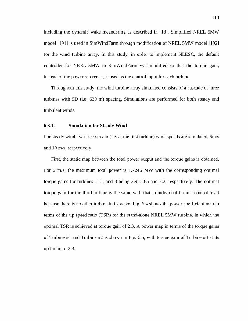
118
including the dynamic wake meandering as described in [18]. Simplified NREL 5MW
model [191] is used in SimWindFarm through modification of NREL 5MW model [192]
for the wind turbine array. In this study, in order to implement NLESC, the default
controller for NREL 5MW in SimWindFarm was modified so that the torque gain,
instead of the power reference, is used as the control input for each turbine.
Throughout this study, the wind turbine array simulated consists of a cascade of three
turbines with 5D (i.e. 630 m) spacing. Simulations are performed for both steady and
turbulent winds.
6.3.1. Simulation for Steady Wind
For steady wind, two free-stream (i.e. at the first turbine) wind speeds are simulated, 6m/s
and 10 m/s, respectively.
First, the static map between the total power output and the torque gains is obtained.
For 6 m/s, the maximum total power is 1.7246 MW with the corresponding optimal
torque gains for turbines 1, 2, and 3 being 2.9, 2.85 and 2.3, respectively. The optimal
torque gain for the third turbine is the same with that in individual turbine control level
because there is no other turbine in its wake. Fig. 6.4 shows the power coefficient map in
terms of the tip speed ratio (TSR) for the stand-alone NREL 5MW turbine, in which the
optimal TSR is achieved at torque gain of 2.3. A power map in terms of the torque gains
of Turbine #1 and Turbine #2 is shown in Fig. 6.5, with torque gain of Turbine #3 at its
optimum of 2.3.

119
Fig. 6.4 Power Coefficient of NREL 5MW with Pitch Angle 0 °
Fig. 6.5 Static Map of Power Capture for Two Cascaded Turbines at 6m/s
0 2 4 6 8 10 12 14 160
0.05
0.1
0.15
0.2
0.25
0.3
0.35
0.4
0.45
0.5
Blade Tip Speed Ratio
Powe
r Coe
fficie
nt
Torque Gain of Turbine 1
Torq
ue G
ain
of T
urbi
ne 2
2.2 2.4 2.6 2.8 3 3.2 3.4 3.6 3.8 42.7
2.75
2.8
2.85
2.9
2.95
3
3.05
3.1
1.708
1.71
1.712
1.714
1.716
1.718
1.72
1.722
1.724

120
For the dither ESC algorithm shown in Fig. 6.2, the dither period is usually chosen 8
to 10 times of the period corresponding to the cut-off frequency of the input dynamics.
The input dynamics for the third turbine (i.e. the stand-alone operated turbine) is
determined by step response test in SimWindFarm simulation, with the torque gain as
input and the power as output. As to be seen later, the input dynamics of power regulation
is a first-order system, without delay for the immediate turbine, while with delay for
downstream turbines. The time constant for the input dynamics without delay is
estimated by linear regression after log transformation of the step response data [8, 193],
which is briefly described below.
For an individual turbine or last one in an array of turbines, a first-order dynamics is
used to approximate its input dynamics between torque gain and power. Its transfer
function could be described as
1( )1IPF s
sτ=
+ (6.10)
Its step response could be described as
/( ) (1 )tout inX t KA e τ−= − (6.11)
If a logarithmic transformation is applied to the system output, we obtained a linear
relation between the transformed output and the time
ln 1 out
in
X tZKA τ
= − = −
(6.12)
where the slope is
1dZdt τ
= − (6.13)
With the recorded data points, the time constant τ can be estimated by linear regression:

121
tZ
τ ∆= −
∆ (6.14)
For the NREL 5MW turbine, the step response of power output under torque-gain
input is shown could be found in Fig. 6.6. Then Z could be calculated by Eq. (6.12), as
shown in Fig. 6.7. By Eq.(6.14), the time constant of input dynamics is 8 second.
Then dither period in ESC for the third turbines is chosen as 80s, which are about 10
times of their respectively period of input dynamics.
Fig. 6.6 Step Response of NREL 5MW Power
400 600 800 1000 1200 1400 1600 1800 20004.2
4.4
4.6
4.8
5
5.2x 10
5
Time (Second)
Gen
erto
r Pow
er 3
(W)
400 600 800 1000 1200 1400 1600 1800 20001
2
3
4
5
Time (Second)
Torq
ue G
ain

122
Fig. 6.7 Estimation of Time Constant of for Torque Based Power Regulation
For the third turbine, the high-pass filter in ESC is
2
2 0.1111 0.0062s
s s+ + (6.15)
while the low-pass filter in ESC is
2
0.00620.1111 0.0062s s+ +
(6.16)
The Bode diagrams of input dynamics, low-pass filter and high-pass filter for the 3rd
turbine is shown in Fig. 6.8. The dither frequency for the 3rd turbine is 0.0785 rad/s. The
phase angle in dither signal for 3rd turbine is chosen as -57.8581Pα = , which results in
( ) ( ) 0P P IP P HP PF j F jθ α ω ω= +∠ +∠ ≈ at this dither frequency.
0 5 10 15 20 25 30 35 400
2
4
6
8
10
12
14
∆t

123
Fig. 6.8 Illustration of ESC Dither Frequency and Phase Compensation for Turbine #3
The input dynamics between torque gain of the second turbine and the power
summation of the 2nd and 3rd turbine could be estimated by first-order dynamics (6.10)
with time delay due to wake transportation, i.e.
22( ) ( )
1
sTsT
IPd IPdeF s e F ssτ
−−= =
+ (6.17)
where T2 is the delay time due to wake transportation.
Similarly, the input dynamics between torque gain of the 1st turbine and the power
summation of the 1st, 2nd and 3rd turbine could also be estimated by Eq. (6.17). The only
difference is that T2 is replaced with T1 the wake transportation time from the 1st turbine
to 3rd turbine.
-100
-80
-60
-40
-20
0
Mag
nitu
de (d
B)
10-3
10-2
10-1
100
101
-180
-90
0
90
180
Phas
e (d
eg)
Bode Diagram
Frequency (rad/sec)
Input Dynamics of 3rd TurbineLow -pass FilterHigh-pass Filter
𝜔3𝑑

124
For the case with wind speed 6m/s at the 1st turbine, wake transportation time from
the second turbine to the third turbine is about 105 second (= 5×126m÷6m/s), which is
lower than actual wake transportation time due to wind deficit after turbines. Similarly,
wake transportation time from 1st turbine to 3rd turbine is 226 (= 113×2) seconds.
Then, the dither periods in ESC for the first and second turbines are chosen as 2800s
and 1400s, which are about 10 times of their respectively period of input dynamics.
For the first turbine, the high-pass filter in ESC is designed as
(6.18)
while the low-pass filter is designed as
(6.19)
The Bode diagram of input dynamics, low-pass filter and high-pass filter for 1st
turbine is shown in Fig. 6.9. Dither frequency for 1st turbine is 0.0022 rad/s. For better
extraction of gradient information, the phase angle is chosen as -59.9144Pα = , which
results in ( ) ( ) 0P P IP P HP PF j F jθ α ω ω= +∠ +∠ ≈ at this dither frequency.
2
2 60.0032 5.0355 10s
s s −+ + ×
6
2 6
5.0355 100.0032 5.0355 10s s
−
−
×+ + ×

125
Fig. 6.9 Illustration of ESC Dither Frequency and Phase Compensation for Turbine #1
For the second turbine, the high-pass filter in ESC is designed as
2
2 50.0063 2.0142 10s
s s −+ + × (6.20)
while the low-pass filter in ESC is
5
2 5
2.0142 100.0063 2.0142 10s s
−
−
×+ + ×
(6.21)
Similarly, the Bode diagrams of input dynamics, low-pass filter and high-pass filter
for the 2nd turbine is shown in Fig. 6.10. The dither frequency for the 2nd turbine is 0.0045
rad/s. For better tracking, the phase angle is chosen as -60.9437Pα = , which results in
( ) ( ) 0P P IP P HP PF j F jθ α ω ω= +∠ +∠ ≈ at this dither frequency.
-120
-100
-80
-60
-40
-20
0
Mag
nitu
de (d
B)
10-4
10-3
10-2
10-1
100
101
-360
-180
0
180
360
Phas
e (d
eg)
Bode Diagram
Frequency (rad/sec)
Input Dynamics for 1st TurbineLow -pass FilterHigh-pass Filter
𝜔1𝑑

126
Fig. 6.10 Illustration of ESC Dither Frequency and Phase Compensation for Turbine #2
For the smooth 6 m/s wind, the forward loop gains for the 1st, 2nd and 3rd turbine are
set at 8×10⁻⁸, 1.5×10⁻⁷ and 1.2×10⁻⁵, respectively. For the 10 m/s case, the forward loop
gains for the 1st, 2nd and 3rd turbines are set as 1×10⁻⁸, 2.5×10⁻⁸ and 1.2×10⁻⁶, respectively.
For steady wind cases, the dither amplitudes are 0.01, 0.01 and 0.05 for 1st, 2nd and 3rd
turbine, respectively.
The torque gains for three turbines are plotted in Fig. 6.11, which shows torque-based
ESC for three turbines are turned on at 400s, 1500s and 3500s, respectively. In current
simulation, the ESC controllers of three turbines are turned on in sequence in order to
better distinguish the associated searching transients. The wind speed profiles at the three
turbines are shown in Fig. 6.12, which reveals that the wind speeds at the second and
-120
-100
-80
-60
-40
-20
0
Mag
nitud
e (d
B)
10-4
10-3
10-2
10-1
100
101
-720
-360
0
360
720
Phas
e (d
eg)
Bode Diagram
Frequency (rad/sec)
Input Dynamics for 2nd TurbineLow -pass FilterHigh-pass Filter
𝜔2𝑑

127
third turbines both increase when the ESC’s for the first and second turbines were turned
on.
Fig. 6.11 Torque Gain Profiles for NLESC Search under 6m/s Smooth Wind
The generator speeds for the three turbines are plotted in Fig. 6.13, which shows that
the generator speed profiles of Turbines 1 and 2 are reduced when their ESC are turned
on. Fig. 6.12 and Fig. 6.13 show that the rotor speeds of upstream turbines are reduced so
that the wind speeds at the downstream turbines increase, and in consequence, the total
power output of the wind farm increases. Fig. 6.14 compares the total power output of the
ESC control with that by use of SimWindFarm’s default controller, which is described in
Appendix G. During the period [10000s, 16000s], the total energy captured increases by
8.7%. During the same period, the average torque gains for the 1st, 2nd and 3rd turbines are
3.02, 2.86 and 2.36, respectively, as compared to the corresponding optimum values of
2.9, 2.85 and 2.3, respectively from the static map.
0 2000 4000 6000 8000 10000 12000 14000 160000.5
1
1.5
2
2.5
3
3.5
Time (Second)
Torq
ue G
ain
1st Turbine2rd Turbine3rd Turbine

128
Fig. 6.12 Wind Speed at Each Turbine for NLESC Search under 6m/s Smooth Wind
Fig. 6.13. Generator Speed Profiles for NLESC Search under 6m/s Smooth Wind
0 2000 4000 6000 8000 10000 12000 14000 16000
5
5.2
5.4
5.6
5.8
6
6.2
6.4
Time (Second)
Effe
ctiv
e W
ind
Spe
ed(m
/s)
1st TurbineESC 2rd TurbineESC 3rd TurbineBenchmark 2rd TurbineBenchmark 3rd Turbine

129
Fig. 6.14. Total Power Profiles for NLESC Search under 6m/s Smooth Wind
Next, the wind speed at the first turbine is increased to 10m/s. Through a 750-second
sweeping simulation, the optimal torque gains of the static power map obtained turn out
to be the same as those for the 6 m/s case, which verifies that the optimal torque gains are
invariant with wind speed. For the NLESC simulation under smooth 10 m/s wind, the
profiles of torque gains, effective wind speed and generator speed are shown in Fig. 6.15,
Fig. 6.16 and Fig. 6.17, respectively.
0 2000 4000 6000 8000 10000 12000 14000 160000
0.5
1
1.5
2
2.5
Time (Second)
Tota
l Pow
er (M
W)
Benchmark ControlESC

130
Fig. 6.15. Torque Gain Profiles for NLESC Search under 10 m/s Smooth Wind
Fig. 6.16. Effective Wind Speed at Each Turbine for NLESC Search under 10 m/s Smooth Wind
0 2000 4000 6000 8000 10000 12000 14000 160001.4
1.6
1.8
2
2.2
2.4
2.6
2.8
3
Time (Second)
Torq
ue G
ain
1st Turbine2rd Turbine3rd Turbine
0 2000 4000 6000 8000 10000 12000 14000 160008.2
8.4
8.6
8.8
9
9.2
9.4
9.6
9.8
10
10.2
Time (Second)
Effe
ctiv
e W
ind
Spee
d(m
/s)
1st TurbineESC 2rd TurbineESC 3rd TurbineBenchmark 2rd TurbineBenchmark 3rd Turbine

131
Fig. 6.17 Generator Speed Profiles for NLESC Search under 10 m/s Smooth Wind
Compared to the benchmark controller, the total power captured was increased by
0.34% during the period [10000s, 16000s], as shown in Fig. 6.18. It seems that the
NLESC yields more benefit in power capture under lower wind speed than high wind
speed (i.e. near the rated wind speed), which is consistent with simulation results in [194].
0 2000 4000 6000 8000 10000 12000 14000 1600050
60
70
80
90
100
110
120
130
Time (Second)
Gen
erat
or S
peed
(rad
/s)
ESC 1st TurbineESC 2rd TurbineESC 3rd TurbineBenchmark 1st TurbineBenchmark 2nd TurbineBenchmark 3rd Turbine

132
Fig. 6.18 Total Power Profiles for ESC Search for Smooth 10 m/s Wind
6.3.2. Turbulent Wind
Simulation was then performed for a turbulent wind case, with the mean wind speed of
8m/s and the turbulent intensity to be 5%. The effective wind speed at the 1st turbine is
the same for both the NLESC and benchmark controllers, as shown in Fig. 6.19. For the
2nd and 3rd turbines, Fig. 6.20 and Fig. 6.21 show that the effective wind speeds with the
NLESC controllers are higher than that with the benchmark controller. The dither
frequencies remain the same as those used in steady wind. The dither amplitudes are 0.05,
0.03 and 0.1 for 1st, 2nd and 3rd turbine, respectively, which are larger than those for the
smooth wind case. The forward-loop gains for the 1st, 2nd and 3rd turbines are 0.1, 0.23
and 1, respectively. The forward-loop gains in turbulent wind cases are much bigger than
those for steady wind cases because power coefficients rather than power are used as
0 2000 4000 6000 8000 10000 12000 14000 160007.5
7.6
7.7
7.8
7.9
8
8.1
8.2
Time (Second)
Tota
l Pow
er (M
W)
Benchmark ControlESC

133
output for the turbulent wind case. The torque gains are plotted in Fig. 6.22. Generator
speeds for 1st, 2nd and 3rd turbine are plotted in Fig. 6.23, Fig. 6.24 and Fig. 6.25,
respectively. Compared to the default controller in SimWindFarm, the energy capture is
increased by 1.3% during the period [10000s, 30000s], as shown in Fig. 6.26.
Fig. 6.19. Effective Wind Speed Profile at Turbine #1 under 8 m/s 5% Turbulent Wind
0 0.5 1 1.5 2 2.5 3
x 104
6.5
7
7.5
8
8.5
9
9.5
10
10.5
Time (Second)
Effe
ctiv
e W
ind
Spee
d at
1st
Tur
bine
(m/s
)
ESCBenchmark

134
Fig. 6.20 Effective Wind Speed Profile at Turbine #2 under 8 m/s 5% Turbulent Wind
Fig. 6.21. Effective Wind Speed Profile at Turbine #3 under 8 m/s 5% Turbulent Wind
0 0.5 1 1.5 2 2.5 3
x 104
5.5
6
6.5
7
7.5
8
8.5
9
9.5
Time (Second)
Effe
ctiv
e W
ind
Spee
d at
2nd
Tur
bine
(m/s
)
ESCBenchmark
0 0.5 1 1.5 2 2.5 3
x 104
5
5.5
6
6.5
7
7.5
8
8.5
9
9.5
Time (Second)
Effe
ctiv
e W
ind
Spee
d at
3rd
Tur
bine
(m/s
)
ESCBenchmark

135
Fig. 6.22. Torque Gains under 8 m/s 5% Turbulent Wind
Fig. 6.23 Generator Speed at Turbine 1 under 8 m/s 5% Turbulent Wind
0 0.5 1 1.5 2 2.5 3
x 104
1.8
2
2.2
2.4
2.6
2.8
3
3.2
Time (Second)
Torq
ue G
ain
1st Turbine2rd Turbine3rd Turbine
0 0.5 1 1.5 2 2.5 3
x 104
50
60
70
80
90
100
110
120
Time (Second)
Gen
erat
or S
peed
of 1
st T
urbi
ne(ra
d/s)
Benchmark ControlESC

136
Fig. 6.24 Generator Speed at Turbine 2 under 8 m/s 5% Turbulent Wind
Fig. 6.25 Generator Speed at Turbine 3 under 8 m/s 5% Turbulent Wind
0 0.5 1 1.5 2 2.5 3
x 104
50
60
70
80
90
100
110
Time (Second)
Gen
erat
or S
peed
of 2
nd T
urbi
ne(ra
d/s)
Benchmark ControlESC
0 0.5 1 1.5 2 2.5 3
x 104
50
60
70
80
90
100
110
Time (Second)
Gen
erat
or S
peed
of 3
rd T
urbi
ne(ra
d/s)
Benchmark ControlESC
137
Fig. 6.26. Total Power under 8 m/s 5% Turbulent Wind
6.4. Conclusion
This part of dissertation study evaluates an NLESC wind farm controller which aims to
maximize the farm-level energy capture. Static mapping under different wind speed
validates the analytical result that the optimal torque gains are invariant with the wind
speed in terms of maximizing the whole-farm power capture. Compared with the default
controller available in SimWindFarm, the effectiveness of the NLESC was verified by
simulation results under both steady and turbulent winds.
0 0.5 1 1.5 2 2.5 3
x 104
0
1
2
3
4
5
6
7
Time (Second)
Tota
l Pow
er (M
W)
Benchmark ControlESC

138
Chapter 7. Active Vane Control for Stabilization of Floating
Offshore Wind Turbine
Control of offshore floating wind turbines has emerged as a much more complicated
problem compared to the land based units. Stabilization and load reduction control are
both important for floating turbines, while such tasks are challenged by underactuation
situation. This chapter evaluates a novel idea [35] for controlling the roll and pitch
motion of floating wind turbines respectively by actively controlled vertical and
horizontal vanes. The structural dynamics of the floating wind turbine with the vane
actuator is simulated through modifying Tail-Furling module in software FAST [140].
Proportional-integral (PI) controllers are applied to control the vane actuators based on
tower pitch or roll motions. While an individual blade pitch controller is designed for
other aspects of wind turbine control. The Hywind platform [195] is adopted for the
simulation model of floating offshore turbine. For the active vane control, different
measurement feedback schemes (including velocity and acceleration on tower top) and
different vane areas are evaluated. Simulation results show that of the roll motion of the
floating turbine can be effectively reduced, and the damage equivalent loads (DEL)
relevant to the side-to-side bending moment at tower base is reduced from 19% to 42%
under turbulent wind with mean speed 18 m/s.
The remainder of this chapter is organized as following. The vertical vane design and
simulation platform is described in Section 7.1, and the horizontal vane design is
described in Section 7.2. Simulation results are presented in Section 7.3.

139
7.1. Vertical Vane Design
7.1.1. Design Approach
Vertical vane actuators are placed at tower top in order to effectively increase damping of
floating turbine tower along side-to-side direction. For wind turbines, significantly high
weight at tower top due to the use of inertial forces leads to difficulty of installation and
maintenance, as well as the high power requirement. The active vertical vane control is
based on the use of the aerodynamic forces which would have higher force-to-weight
ratio and leads to lower cost, compared to heavier TMD (Tuned Mass-Spring Damper)
[33].
Besides, the active vertical vane design requires the use of downwind turbine design;
otherwise the active vertical vane would reside in the near wake of the wind turbine rotor
and its aerodynamic behavior would be intractable. For land based wind turbines,
upwind design is typically preferred over downwind design as downwind design leads to
the shadow effect that leads to significant periodic fatigue load and power fluctuation.
However, for offshore wind turbines, reducing blade weight is of higher benefit, and thus
downwind design has received better acceptance because lighter blades can be used when
blade-tower collision is not a concern. Side view and top view of downwind wind
turbines including vertical vanes are shown in Fig. 7.1.
7.1.2. Simulation Platform for Vertical Vane
Jonkman [196] developed an aeroelastic model of a small furling wind turbine by use of
the Kane’s method [197] and implemented it in FAST [140]. In this study, the tail-furling
module in FAST is modified to simulate the vane actuator. In the furling input files, tail-
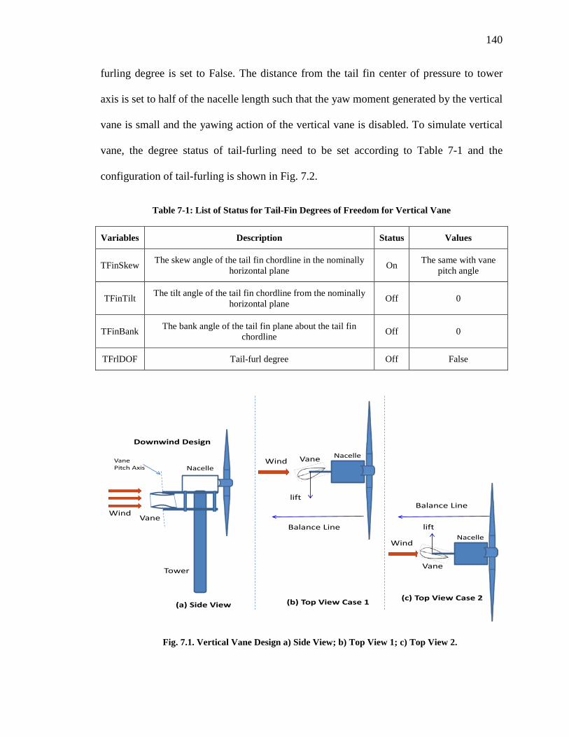
140
furling degree is set to False. The distance from the tail fin center of pressure to tower
axis is set to half of the nacelle length such that the yaw moment generated by the vertical
vane is small and the yawing action of the vertical vane is disabled. To simulate vertical
vane, the degree status of tail-furling need to be set according to Table 7-1 and the
configuration of tail-furling is shown in Fig. 7.2.
Table 7-1: List of Status for Tail-Fin Degrees of Freedom for Vertical Vane
Variables Description Status Values
TFinSkew The skew angle of the tail fin chordline in the nominally horizontal plane On The same with vane
pitch angle
TFinTilt The tilt angle of the tail fin chordline from the nominally horizontal plane Off 0
TFinBank The bank angle of the tail fin plane about the tail fin chordline Off 0
TFrlDOF Tail-furl degree Off False
Fig. 7.1. Vertical Vane Design a) Side View; b) Top View 1; c) Top View 2.
Downwind Design
Tower
Vane
VanePitch Axis
Wind
(b) Top View Case 1
Balance Linelift
WindNacelleVane
lift
WindNacelle
Vane
(a) Side View(c) Top View Case 2
Balance Line
Nacelle

141
Fig. 7.2. Configuration of Tail-Furling
Originally tail-furling is passively controlled in FAST. The working principle of
passive-controlled tail-furling is:
a) When wind speed is above rated wind speed, the rotor is yawed and/or tilted out of
wind direction due to higher thrust loading on the rotor;
b) When wind speed is below rated wind speed, the rotor is returned to wind direction
due to lower thrust loading on the rotor;
In this study, the active control input of vertical vane is the vane pitch angle, which is
defined as the angle between nominal downwind direction and the plane composed of
vertical vane’s airfoil chord lines. In FAST, the angle TFinSkew stands for vertical vane
pitch angle. To facilitate the controller design, we modified FAST subroutines related
with variable TFinSkew and rebuilt the Simulink interface of FAST including vane pitch
control, shown in Fig. 7.3.
Figure by Jason Jonkman/ NREL

142
Fig. 7.3. Simulink Interface of FAST including Vertical Vane Pitch Control.
7.1.3. Airfoils for Vertical Vane
When wind turbine is located at the equilibrium point along the side-to-side direction, it
is desirable not to have aerodynamic forces generated by the vertical vane. Therefore,
symmetrical airfoils or symmetrical pair of airfoils should be used. In this study,
symmetrical airfoil NACA0012 is used, and its aerodynamic characteristics can be found
in a report by Sandia National Laboratory [198]. The lift and drag coefficients of
NACA0012 are plotted in Fig. 7.4. To achieve tractable control action, stall operation is
avoided. The range of angle of attack for nearly linear lift characteristics (no stall) is from
−20° to 20°. In order to fully test the capability of vertical vane to stabilize floating
turbine in side-to-side direction, a high-lift airfoil [199] is also used and its aerodynamic
coefficients were modified to simulate a pair of high-lift airfoils for symmetry
achievement.
7.1.4. Controller Design of Floating Offshore Turbine with Vertical Vane
Control
In this study, blade pitch control, generator torque control and vertical vane pitch control
are considered. The objective is to compare the wind turbine performance with and

143
without the vertical vane control so that the effectiveness of the active vane control can
be evaluated.
Fig. 7.4. Lift and Drag Coefficients of NACA0012
Jonkman [195] redesigned PI-based blade pitch controller for floating turbine with
Hywind platform based on his previous work [192] and suggestion from Larsen and
Hansen [32] about negative damping for the tower pitch motion. Such PI pitch controller
[195] and PI-based Individual pitch controllers [10] are implemented together as the
benchmark of collective pitch control in this chapter.
For the generator torque control, different wind turbine operation regions correspond
to different control modes. Below the rated wind speed, the generator torque is designed
to be proportional to the square of generator speed. Above the rated wind speed, the
generator torque is equal to rated power output over the product of generator speed and
generator efficiency.
-150 -100 -50 0 50 100 150-1.5
-1
-0.5
0
0.5
1
1.5
2
Angle of Attack (degree)
Coef
ficie
nt
Lift CoefficientDrag Coefficient

144
The PI-based vertical vane controllers are designed based on different measurements
including the side-to-side velocity and side-to-side acceleration at the tower top. The
controller loop including vertical vane control is shown in Fig. 7.5.
Fig. 7.5. Vertical Vane Control Loop
7.2. Horizontal Vane Design
In order to stabilize the pitch motion of floating turbine, a horizontal vane is proposed in
[35] to increase tower damping of pitch motion. A simple treatment is to put the
horizontal vane under the nacelle bedplate as the way of installing the vertical vane, but
the moment arm length thus resulted would be insufficient. Based on this situation, a
horizontal vane is placed at tower base, which is shown in Fig. 7.6.
FAST
PI Controller
Side-Side Velocity on Tower Top
Pitch Actuator Dynamics
PI Controller
Rotor SpeedFlapwiseMomentsAt Blade Roots
Coleman Transformation
D axis Controller
Q axis Controller
Inverse of Coleman
Transformation+
(Wind Turbine Simulator)Generator Torque
Individual Blade Pitch Input
Vane Pitch Input

145
Fig. 7.6. Configuration of Horizontal Vane
Horizontal vane is also simulated through modifying Tail-Furling module of FAST
software. Settings of FAST input for tail fin are listed in Table 7-2. For horizontal vane
control, a new FAST Simulink interface is also built for controller design.
Table 7-2: FAST Setting for Horizontal Vane
Variables Description On/Off Values
TFinSkew The skew angle of the tail fin chordline in the nominally horizontal plane On 0
TFinTilt The tilt angle of the tail fin chordline from the nominally horizontal plane Off The same with horizontal
vane pitch angle
TFinBank The bank angle of the tail fin plane about the tail fin chordline Off 90 degree
TFrlDOF Tail-furl degree Off False
PI-based horizontal vane controllers are designed based on the measurement of fore-
aft velocity and acceleration on tower top. The whole controller loop including horizontal
VaneWind Vane
Pitch Motion
Wind
Sea level
Velocity at Tower Top Velocity at Tower Top
Negative Half Cycle Positive Half Cycle
Balance Line
Balance Line
Pitch Motion
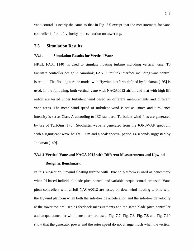
146
vane control is nearly the same to that in Fig. 7.5 except that the measurement for vane
controller is fore-aft velocity or acceleration on tower top.
7.3. Simulation Results
7.3.1. Simulation Results for Vertical Vane
NREL FAST [140] is used to simulate floating turbine including vertical vane. To
facilitate controller design in Simulink, FAST Simulink interface including vane control
is rebuilt. The floating turbine model with Hywind platform defined by Jonkman [195] is
used. In the following, both vertical vane with NACA0012 airfoil and that with high lift
airfoil are tested under turbulent wind based on different measurements and different
vane areas. The mean wind speed of turbulent wind is set as 18m/s and turbulence
intensity is set as Class A according to IEC standard. Turbulent wind files are generated
by use of TurbSim [176]. Stochastic wave is generated from the JONSWAP spectrum
with a significant wave height 3.7 m and a peak spectral period 14 seconds suggested by
Jonkman [149].
7.3.1.1.Vertical Vane and NACA 0012 with Different Measurements and Upwind
Design as Benchmark
In this subsection, upwind floating turbine with Hywind platform is used as benchmark
when PI-based individual blade pitch control and variable torque control are used. Vane
pitch controllers with airfoil NACA0012 are tested on downwind floating turbine with
the Hywind platform when both the side-to-side acceleration and the side-to-side velocity
at the tower top are used as feedback measurements and the same blade pitch controller
and torque controller with benchmark are used. Fig. 7.7, Fig. 7.8, Fig. 7.8 and Fig. 7.10
show that the generator power and the rotor speed do not change much when the vertical

147
vane control is used. Fig. 7.11 and Fig. 7.12 show that the side-to-side velocity at the
tower top is significantly alleviated when the vertical vane control is used. Compared
with the case when the side-to-side acceleration at the tower top is used as feedback, the
side-to-side velocity at the tower top is further reduced when the side-to-side velocity at
the tower top is used as feedback.
Fig. 7.13 and Fig. 7.14 show that the vane pitch angle has more activity at high
frequency when the side-to-side acceleration is used as measurement. Fig. 7.15, Fig. 7.16,
Fig. 7.17, Fig. 7.18, Fig. 7.19 and Fig. 7.20 show that the platform translational sway
displacement, the roll displacement and the side-to-side moment are reduced when both
side-to-side velocity and acceleration at tower top are used as measurement. Compared
with the case when acceleration feedback is used, displacement and loads are further
reduced when velocity is used as measurement.

148
Fig. 7.7. Generator Power (Vertical Vane, NACA0012, Upwind as Benchmark)
Fig. 7.8 Spectra of Generator Power (Vertical Vane, NACA0012, Upwind as Benchmark)
100 200 300 400 500 600 7003400
3600
3800
4000
4200
4400
4600
4800
5000
5200
Time (Second)
Gen
erat
or P
ower
(kW
)
Without Vertical Vane ControlAcceleration Measurement at Tower TopVelocity Measurement at Tower Top
0 0.1 0.2 0.3 0.4 0.5 0.60
100
200
300
400
500
600
Frequency (Hz)
Gene
rato
r Pow
er(k
W)
Without Vertical Vane ControlAcceleration Measurement at Tower TopVelocity Measurement at Tower Top

149
Fig. 7.9. Rotor Speed (Vertical Vane, NACA0012, Upwind as Benchmark)
Fig. 7.10. Spectra of Rotor Speed (Vertical Vane, NACA0012, Upwind as Benchmark)
100 200 300 400 500 600 7007
8
9
10
11
12
13
14
15
16
17
Time (Second)
Rot
or S
peed
(rpm
)
Without Vertical Vane ControlAcceleration Measurement at Tower TopVelocity Measurement at Tower Top
0 0.1 0.2 0.3 0.4 0.5 0.60
5
10
15
20
25
Frequency (Hz)
Rot
or S
peed
(rpm
)
Without Vertical Vane ControlAcceleration Measurement at Tower TopVelocity Measurement at Tower Top

150
Fig. 7.11. Side-to-Side Velocity (Vertical Vane, NACA0012, Upwind as Benchmark)
Fig. 7.12. Spectra of Side-to-Side Velocity (Vertical Vane, NACA0012, Upwind as Benchmark)
100 200 300 400 500 600 700-1.5
-1
-0.5
0
0.5
1
1.5
Time (Second)
Side
-to-S
ide
Velo
city
on
Towe
r Top
(m/s
)
Without Vertical Vane ControlAcceleration Measurement at Tower TopVelocity Measurement at Tower Top
0 0.1 0.2 0.3 0.4 0.5 0.60
0.1
0.2
0.3
0.4
0.5
0.6
0.7
Frequency (Hz)
Side
-to-S
ide
Velo
city
on
Tow
er T
op(m
/s)
Without Vertical Vane ControlAcceleration Measurement at Tower TopVelocity Measurement at Tower Top

151
Fig. 7.13. Vane Pitch Angle (Vertical Vane, NACA0012, Upwind as Benchmark)
Fig. 7.14. Spectra of Vane Pitch Angle (Vertical Vane, NACA0012, Upwind as Benchmark)
400 420 440 460 480 500 520 540 560 580 600-20
-15
-10
-5
0
5
10
15
20
Time (Second)
Vane
Pitc
h An
gle(
degr
ee)
Without Vertical Vane ControlAcceleration Measurement at Tower TopVelocity Measurement at Tower Top
0 0.1 0.2 0.3 0.4 0.5 0.60
1
2
3
4
5
6
7
Frequency (Hz)
Van
e P
itch
Ang
le (d
egre
e)
Without Vertical Vane ControlAcceleration Measurement at Tower TopVelocity Measurement at Tower Top

152
Fig. 7.15. Platform Sway Displacement (Vertical Vane, NACA0012, Upwind as Benchmark)
Fig. 7.16. Platform Sway Displacement Spectra (Vertical, NACA0012, Upwind as Benchmark)
100 200 300 400 500 600 700-4
-3
-2
-1
0
1
2
Time (Second)
Plat
form
Tra
nsla
tiona
l Swa
y Di
spla
cem
ents
(m)
Without Vertical Vane ControlAcceleration Measurement at Tower TopVelocity Measurement at Tower Top
0 0.1 0.2 0.3 0.4 0.5 0.60
0.2
0.4
0.6
0.8
1
1.2
1.4
Frequency (Hz)
Plat
form
Tra
nsla
tiona
l Sw
ay D
ispl
acem
ents
(m)
Without Vertical Vane ControlAcceleration Measurement at Tower TopVelocity Measurement at Tower Top

153
Fig. 7.17. Platform Roll Displacement (Vertical Vane, NACA0012, Upwind as Benchmark)
Fig. 7.18. Platform Roll Displacement Spectra (Vertical, NACA0012, Upwind as Benchmark)
100 200 300 400 500 600 700-2
-1.5
-1
-0.5
0
0.5
1
1.5
2
Time (Second)
Plat
form
rol
l dis
plac
emen
ts(d
egre
e)
Without Vertical Vane ControlAcceleration Measurement at Tower TopVelocity Measurement at Tower Top
0 0.1 0.2 0.3 0.4 0.5 0.60
0.1
0.2
0.3
0.4
0.5
0.6
0.7
0.8
0.9
1
Frequency (Hz)
Plat
form
rota
tiona
l rol
l dis
plac
emen
ts(d
egre
e)
Without Vertical Vane ControlAcceleration Measurement at Tower TopVelocity Measurement at Tower Top

154
Fig. 7.19. Side-to-Side Bending Moment (Vertical Vane, NACA0012, Upwind as Benchmark)
Fig. 7.20. Side-to-Side Bending Moment Spectra (Vertical, NACA0012, Upwind as Benchmark)
100 200 300 400 500 600 700-3
-2
-1
0
1
2
3
4x 10
4
Time (Second)
Side
-to-s
ide
Bend
ing
Mom
ents
at t
he to
wer b
ase
(kN*
m)
Without Vertical Vane ControlAcceleration Measurement at Tower TopVelocity Measurement at Tower Top
0 0.1 0.2 0.3 0.4 0.5 0.60
2000
4000
6000
8000
10000
12000
Frequency (Hz)Sid
e-to
-sid
e B
endi
ng M
omen
ts a
t the
tow
er b
ase
(kN
*m)
Without Vertical Vane ControlAcceleration Measurement at Tower TopVelocity Measurement at Tower Top

155
7.3.1.2. Vertical Vane and NACA 0012 with Different Measurements and
Downwind Design as Benchmark
Similar to the previous section, downwind floating turbine with Hywind platform is used
as benchmark when PI-based individual blade pitch control and variable torque control
are used. Vane pitch controllers with airfoil NACA0012 are tested on downwind floating
turbine with Hywind platform when both the side-to-side acceleration and the side-to-
side velocity at tower top are used as measurements and the same blade pitch controller
and torque controller with benchmark are used. Fig. 7.21 through Fig. 7.24 show that
generator power and rotor speed do not change a lot when vertical vane control is used.
Fig. 7.25 and Fig. 7.26 show that the vane pitch angle has more activity at high
frequency when side-to-side acceleration is used as measurement. Fig. 7.27 and Fig. 7.28
show that side-to-side velocity at tower top is significantly alleviated when vertical vane
control is used. Compared with that when side-to-side acceleration at tower top is used as
measurement, side-to-side velocity at tower top is further reduced when side-to-side
velocity at tower top is used as measurement. Similarly, Fig. 7.29 through Fig. 7.34 show
that the platform sway displacement, the roll displacement and the side-to-side moment
are reduced when both velocity and acceleration are used as measurement. Compared
with that when acceleration is used as measurement, displacement and loads are further
reduced when velocity is used as measurement.

156
Fig. 7.21. Generator Power (Vertical Vane, NACA0012, Downwind as Benchmark)
Fig. 7.22. Generator Power Spectra (Vertical Vane, NACA0012, Downwind as Benchmark)
100 200 300 400 500 600 7003400
3600
3800
4000
4200
4400
4600
4800
5000
5200
5400
Time (Second)
Gen
erat
or P
ower
(kW
)
Without Vertical Vane ControlAcceleration Measurement at Tower TopVelocity Measurement at Tower Top
0 0.1 0.2 0.3 0.4 0.5 0.60
100
200
300
400
500
600
Frequency (Hz)
Gen
erat
or P
ower
(kW
)
Without Vertical Vane ControlAcceleration Measurement at Tower TopVelocity Measurement at Tower Top

157
Fig. 7.23. Rotor Speed (Vertical Vane, NACA0012, Downwind as Benchmark)
Fig. 7.24. Rotor Speed Spectra (Vertical Vane, NACA0012, Downwind as Benchmark)
100 200 300 400 500 600 7007
8
9
10
11
12
13
14
15
16
17
Time (Second)
Roto
r Spe
ed (r
pm)
Without Vertical Vane ControlAcceleration Measurement at Tower TopVelocity Measurement at Tower Top
0 0.1 0.2 0.3 0.4 0.5 0.60
5
10
15
20
25
Frequency (Hz)
Rot
or S
peed
(rpm
)
Without Vertical Vane ControlAcceleration Measurement at Tower TopVelocity Measurement at Tower Top

158
Fig. 7.25. Vane Pitch Angle (Vertical Vane, NACA0012, Downwind as Benchmark)
Fig. 7.26. Vane Pitch Angle Spectra (Vertical Vane, NACA0012, Downwind as Benchmark)
400 410 420 430 440 450 460 470 480 490 500-20
-15
-10
-5
0
5
10
15
20
Time (Second)
Vane
Pitc
h An
gle(
degr
ee)
Without Vertical Vane ControlAcceleration Measurement at Tower TopVelocity Measurement at Tower Top
0 0.1 0.2 0.3 0.4 0.5 0.60
1
2
3
4
5
6
7
Frequency (Hz)
Vane
Pitc
h An
gle
(deg
ree)
Without Vertical Vane ControlAcceleration Measurement at Tower TopVelocity Measurement at Tower Top
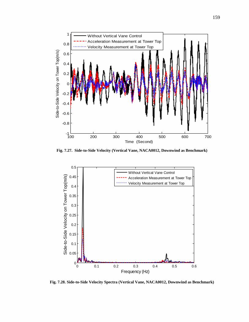
159
Fig. 7.27. Side-to-Side Velocity (Vertical Vane, NACA0012, Downwind as Benchmark)
Fig. 7.28. Side-to-Side Velocity Spectra (Vertical Vane, NACA0012, Downwind as Benchmark)
100 200 300 400 500 600 700-1
-0.8
-0.6
-0.4
-0.2
0
0.2
0.4
0.6
0.8
1
Time (Second)
Side
-to-S
ide
Velo
city
on
Towe
r Top
(m/s
)
Without Vertical Vane ControlAcceleration Measurement at Tower TopVelocity Measurement at Tower Top
0 0.1 0.2 0.3 0.4 0.5 0.60
0.05
0.1
0.15
0.2
0.25
0.3
0.35
0.4
0.45
0.5
Frequency (Hz)
Sid
e-to
-Sid
e V
eloc
ity o
n To
wer
Top
(m/s
)
Without Vertical Vane ControlAcceleration Measurement at Tower TopVelocity Measurement at Tower Top

160
Fig. 7.29. Roll Displacement (Vertical Vane, NACA0012, Downwind as Benchmark)
Fig. 7.30. Roll Displacement Spectra (Vertical Vane, NACA0012, Downwind as Benchmark)
100 200 300 400 500 600 700-1.5
-1
-0.5
0
0.5
1
1.5
2
Time (Second)
Plat
form
rol
l dis
plac
emen
ts(d
egre
e)
Without Vertical Vane ControlAcceleration Measurement at Tower TopVelocity Measurement at Tower Top
0 0.1 0.2 0.3 0.4 0.5 0.60
0.1
0.2
0.3
0.4
0.5
0.6
0.7
0.8
0.9
Frequency (Hz)
Plat
form
rota
tiona
l rol
l dis
plac
emen
ts(d
egre
e)
Without Vertical Vane ControlAcceleration Measurement at Tower TopVelocity Measurement at Tower Top

161
Fig. 7.31. Sway Displacement (Vertical Vane, NACA0012, Downwind as Benchmark)
Fig. 7.32. Sway Displacement Spectra (Vertical Vane, NACA0012, Downwind as Benchmark)
100 200 300 400 500 600 700-4
-3
-2
-1
0
1
2
Time (Second)
Plat
form
Tra
nsla
tiona
l Swa
y Di
spla
cem
ents
(m)
Without Vertical Vane ControlAcceleration Measurement at Tower TopVelocity Measurement at Tower Top
0 0.1 0.2 0.3 0.4 0.5 0.60
0.2
0.4
0.6
0.8
1
1.2
1.4
Frequency (Hz)
Plat
form
Tra
nsla
tiona
l Sw
ay D
ispl
acem
ents
(m)
Without Vertical Vane ControlAcceleration Measurement at Tower TopVelocity Measurement at Tower Top
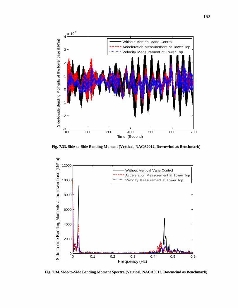
162
Fig. 7.33. Side-to-Side Bending Moment (Vertical, NACA0012, Downwind as Benchmark)
Fig. 7.34. Side-to-Side Bending Moment Spectra (Vertical, NACA0012, Downwind as Benchmark)
100 200 300 400 500 600 700-3
-2
-1
0
1
2
3
4x 10
4
Time (Second)
Side
-to-s
ide
Bend
ing
Mom
ents
at t
he to
wer b
ase
(kN*
m)
Without Vertical Vane ControlAcceleration Measurement at Tower TopVelocity Measurement at Tower Top
0 0.1 0.2 0.3 0.4 0.5 0.60
2000
4000
6000
8000
10000
12000
Frequency (Hz)Side
-to-s
ide
Bend
ing
Mom
ents
at t
he to
wer
bas
e (k
N*m
)
Without Vertical Vane ControlAcceleration Measurement at Tower TopVelocity Measurement at Tower Top

163
7.3.1.3. Vertical Vane and NACA 0012 with Different Vane Area and Downwind
Design as Benchmark
In this subsection, the vane pitch controllers with different vane areas are tested on
downwind floating turbine when side-to-side velocity at tower top is used as the
measurement and airfoil NACA0012 is used. A downwind floating turbine with PI-based
IPC and variable torque controller is used as benchmark. Figures 7.33 through 7.36 show
that the generator power and the rotor speed do not change a lot when vertical vane
control is used.
Fig. 7.39 and Fig. 7.40 show that the vane pitch angle has more variation when vane
area is smaller, i.e. more control actions. Fig. 7.41 and Fig. 7.42 show that the side-to-
side velocity at the tower top is significantly alleviated when the vertical vane control is
used. The bigger the vane area is, the more reduction of the side-to-side velocity at the
tower top is. Fig. 7.43 through Fig. 7.48 show that the roll displacement, the platform
sway displacement, and side-to-side moment are significantly reduced. In summary, the
bigger the vane area is, the more reduction of displacement or loads in side-to-side
direction is.

164
Fig. 7.35. Generator Power (Vertical Vane, NACA0012, Downwind as Benchmark)
Fig. 7.36. Generator Power (Vertical Vane, NACA0012, Downwind as Benchmark)
100 200 300 400 500 600 7003400
3600
3800
4000
4200
4400
4600
4800
5000
5200
5400
Time (Second)
Gen
erat
or P
ower
(kW
)
Without Vertical Vane Control
Vane Control 25 m2
Vane Control 50 m2
Vane Control 100 m2
0 0.1 0.2 0.3 0.4 0.5 0.60
50
100
150
200
250
300
350
400
450
500
Frequency (Hz)
Gen
erat
or P
ower
(kW
)
Without Vertical Vane Control
Vane Control 25 m2
Vane Control 50 m2
Vane Control 100 m2

165
Fig. 7.37. Rotor Speed (Vertical Vane, NACA0012, Downwind as Benchmark)
Fig. 7.38. Rotor Speed Spectra (Vertical Vane, NACA0012, Downwind as Benchmark)
100 200 300 400 500 600 7007
8
9
10
11
12
13
14
15
16
17
Time (Second)
Roto
r Spe
ed (r
pm)
Without Vertical Vane Control
Vane Control 25 m2
Vane Control 50 m2
Vane Control 100 m2
0 0.1 0.2 0.3 0.4 0.5 0.60
0.5
1
1.5
2
2.5
3
3.5
4
4.5
5
Frequency (Hz)
Rot
or S
peed
(rpm
)
Without Vertical Vane Control
Vane Control 25 m2
Vane Control 50 m2
Vane Control 100 m2

166
Fig. 7.39. Vane Pitch Angle (Vertical Vane, NACA0012, Downwind as Benchmark)
Fig. 7.40. Vane Pitch Angle Spectra (Vertical Vane, NACA0012, Downwind as Benchmark)
100 200 300 400 500 600 700-20
-15
-10
-5
0
5
10
15
20
Time (Second)
Vane
Pitc
h An
gle(d
egre
e)
Without Vertical Vane Control
Vane Control 25 m2
Vane Control 50 m2
Vane Control 100 m2
0 0.1 0.2 0.3 0.4 0.5 0.60
2
4
6
8
10
12
14
Frequency (Hz)
Vane
Pitc
h An
gle
(deg
ree)
Without Vertical Vane Control
Vane Control 25 m2
Vane Control 50 m2
Vane Control 100 m2
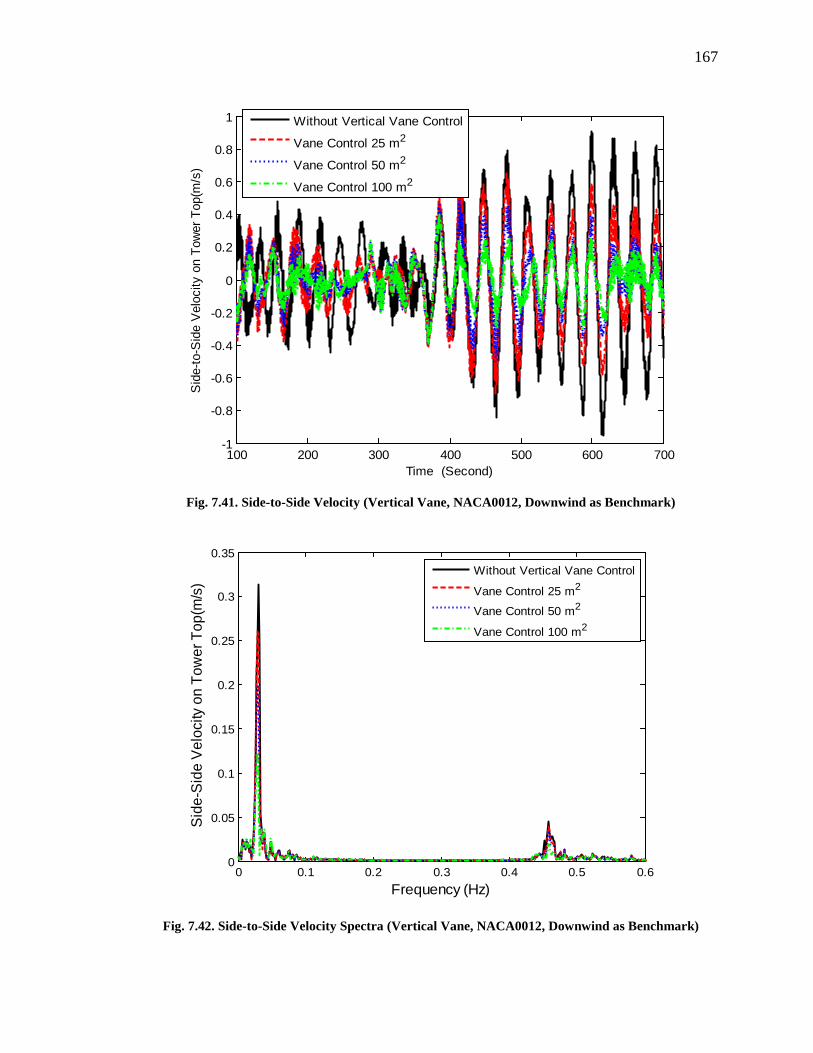
167
Fig. 7.41. Side-to-Side Velocity (Vertical Vane, NACA0012, Downwind as Benchmark)
Fig. 7.42. Side-to-Side Velocity Spectra (Vertical Vane, NACA0012, Downwind as Benchmark)
100 200 300 400 500 600 700-1
-0.8
-0.6
-0.4
-0.2
0
0.2
0.4
0.6
0.8
1
Time (Second)
Sid
e-to
-Sid
e V
eloc
ity o
n To
wer
Top
(m/s
)
Without Vertical Vane Control
Vane Control 25 m2
Vane Control 50 m2
Vane Control 100 m2
0 0.1 0.2 0.3 0.4 0.5 0.60
0.05
0.1
0.15
0.2
0.25
0.3
0.35
Frequency (Hz)
Side
-Sid
e Ve
loci
ty o
n To
wer
Top
(m/s
)
Without Vertical Vane Control
Vane Control 25 m2
Vane Control 50 m2
Vane Control 100 m2

168
Fig. 7.43 Roll Displacement (Vertical Vane, NACA0012, Downwind as Benchmark)
Fig. 7.44. Roll Displacement Spectra (Vertical Vane, NACA0012, Downwind as Benchmark)
100 200 300 400 500 600 700-1.5
-1
-0.5
0
0.5
1
1.5
2
Time (Second)
Plat
form
rota
tiona
l rol
l dis
plac
emen
ts(d
egre
e)
Without Vertical Vane Control
Vane Control 25 m2
Vane Control 50 m2
Vane Control 100 m2
0 0.1 0.2 0.3 0.4 0.5 0.60
0.1
0.2
0.3
0.4
0.5
0.6
0.7
Frequency (Hz)
Plat
form
rota
tiona
l rol
l dis
plac
emen
ts(d
egre
e)
Without Vertical Vane Control
Vane Control 25 m2
Vane Control 50 m2
Vane Control 100 m2

169
Fig. 7.45. Sway Displacement (Vertical Vane, NACA0012, Downwind as Benchmark)
Fig. 7.46 Sway Displacement Spectra (Vertical Vane, NACA0012, Downwind as Benchmark)
100 200 300 400 500 600 700-4
-3
-2
-1
0
1
2
Time (Second)
Pla
tform
Tra
nsla
tiona
l Sw
ay D
ispl
acem
ents
(m)
Without Vertical Vane Control
Vane Control 25 m2
Vane Control 50 m2
Vane Control 100 m2
0 0.1 0.2 0.3 0.4 0.5 0.60
0.1
0.2
0.3
0.4
0.5
0.6
0.7
Frequency (Hz)
Plat
form
Tra
nsla
tiona
l Sw
ay D
ispl
acem
ents
(m)
Without Vertical Vane Control
Vane Control 25 m2
Vane Control 50 m2
Vane Control 100 m2

170
Fig. 7.47. Side-to-Side Bending Moment (Vertical Vane, NACA0012, Downwind as Benchmark)
Fig. 7.48. Side-to-Side Bending Moment (Vertical Vane, NACA0012, Downwind as Benchmark)
100 200 300 400 500 600 700-3
-2
-1
0
1
2
3
4x 10
4
Time (Second)
Side
-to-s
ide
Bend
ing
Mom
ents
at t
he to
wer b
ase
(kN*
m)
Without Vertical Vane Control
Vane Control 25 m2
Vane Control 50 m2
Vane Control 100 m2
0 0.1 0.2 0.3 0.4 0.5 0.60
2000
4000
6000
8000
10000
12000
Frequency (Hz)Side
-to-s
ide
Bend
ing
Mom
ents
at t
he to
wer
bas
e (k
N*m
)
Without Vertical Vane Control
Vane Control 25 m2
Vane Control 50 m2
Vane Control 100 m2

171
7.3.1.4. High Lift Airfoil and Vertical Vane with Different Measurements and
Downwind Design as Benchmark
In this subsection, the vane pitch controllers with a highlift airfoil are tested on
downwind floating turbine with Hywind platform when both side-to-side acceleration and
side-to-side velocity at tower top are used as measurements. Downwind floating turbine
with Hywind platform is used as benchmark when PI-based IPC and variable torque
control are used. Fig. 7.49 through Fig. 7.52 show that the generator power and rotor
speed do not change a lot when vertical vane control is used. Fig. 7.53 and Fig. 7.54 show
that, compared with the vane control with traditional NACA0012 airfoil, variation of
side-to-side velocity at tower top is further reduced when a highlift airfoil is used. Vane
pitch angle and its spectral is shown in Fig. 7.55 and Fig. 7.56.
Figures 7.55 through 7.60 show that platform translational roll displacement, sway
displacement and side-to-side moment are further reduced when a high-lift airfoil is used
and both the velocity and the acceleration along side-to-side direction at tower top are
used as measurement. Compared with that when the acceleration is used as measurement,
the sway displacement and loads are further reduced when the velocity is used as the
measurement.

172
Fig. 7.49. Generator Power Comparison (Vertical Vane, Highlift Airfoil, Downwind as
Benchmark)
Fig. 7.50 Generator Power Spectral (Vertical Vane, Highlift Airfoil, Downwind as Benchmark)
100 200 300 400 500 600 7003400
3600
3800
4000
4200
4400
4600
4800
5000
5200
Time (Second)
Gen
erat
or P
ower
(kW
)
Without Vertical Vane ControlAcceleration Measurement at Tower TopVelocity Measurement at Tower Top
0 0.1 0.2 0.3 0.4 0.5 0.60
1000
2000
3000
4000
5000
6000
7000
8000
9000
10000
Frequency (Hz)
Gen
erat
or P
ower
(kW
)
Without Vertical Vane ControlAcceleration Measurement at Tower TopVelocity Measurement at Tower Top

173
Fig. 7.51 Rotor Speed (Vertical Vane, Highlift Airfoil, Downwind as Benchmark)
Fig. 7.52 Rotor Speed Spectra (Vertical Vane, Highlift Airfoil, Downwind as Benchmark)
100 200 300 400 500 600 7007
8
9
10
11
12
13
14
15
16
17
Time (Second)
Roto
r Spe
ed (r
pm)
Without Vertical Vane ControlAcceleration Measurement at Tower Velocity Measurement at Tower Top
0 0.1 0.2 0.3 0.4 0.5 0.60
5
10
15
20
25
Frequency (Hz)
Roto
r Spe
ed(rp
m)
Without Vertical Vane ControlAcceleration Measurement at Tower TopVelocity Measurement at Tower Top

174
Fig. 7.53 Side-to-side Velocity on Tower Top (Vertical Vane, Highlift Airfoil, Downwind as
Benchmark)
Fig. 7.54 Spectra of Side-to-side Velocity on Tower Top (Vertical Vane, Highlift Airfoil, Downwind
as Benchmark)
100 200 300 400 500 600 700-1.5
-1
-0.5
0
0.5
1
Time (Second)
Side
-to-S
ide V
elocit
y on
Tow
er T
op(m
/s)
Without Vertical Vane ControlAcceleration Measurement at Tower TopVelocity Measurement at Tower Top
0 0.1 0.2 0.3 0.4 0.5 0.60
0.05
0.1
0.15
0.2
0.25
0.3
0.35
0.4
0.45
0.5
Frequency (Hz)
Side
-to-S
ide
Velo
city o
n To
wer T
op(m
/s)
Without Vertical Vane ControlAcceleration Measurement at Tower TopVelocity Measurement at Tower Top

175
Fig. 7.55 Vane Pitch Angle (Vertical Vane, Highlift Airfoil, Downwind as Benchmark)
Fig. 7.56 Vane Pitch Angle Spectra (Vertical Vane, Highlift Airfoil, Downwind as Benchmark)
100 200 300 400 500 600 700-20
-15
-10
-5
0
5
10
15
Time (Second)
Vane
Pitc
h An
gle(
degr
ee)
Without Vertical Vane ControlAcceleration Measurement at Tower TopVelocity Measurement at Tower Top
0 0.1 0.2 0.3 0.4 0.5 0.60
1
2
3
4
5
6
Frequency (Hz)
Vane
Pitc
h An
gle
(deg
ree)
Without Vertical Vane ControlAcceleration Measurement at Tower TopVelocity Measurement at Tower Top

176
Fig. 7.57 Platform Roll Displacement (Vertical Vane, Highlift Airfoil, Downwind as Benchmark)
Fig. 7.58 Platform Roll Displacement Spectra (Vertical Vane, Highlift Airfoil, Downwind as
Benchmark)
100 200 300 400 500 600 700-2
-1.5
-1
-0.5
0
0.5
1
1.5
2
Time (Second)
Plat
form
roll
disp
lacem
ents
(deg
ree)
Without Vertical Vane ControlAcceleration Measurement at Tower TopVelocity Measurement at Tower Top
0 0.1 0.2 0.3 0.4 0.5 0.60
0.1
0.2
0.3
0.4
0.5
0.6
0.7
0.8
0.9
Frequency (Hz)
Plat
form
rota
tiona
l rol
l disp
lace
men
ts(de
gree
)
Without Vertical Vane ControlAcceleration Measurement at Tower TopVelocity Measurement at Tower Top

177
Fig. 7.59 Platform Sway Displacement (Vertical Vane, Highlift Airfoil, Downwind as Benchmark)
Fig. 7.60 Platform Sway Displacement Spectra (Vertical Vane, Highlift Airfoil, Downwind as
Benchmark)
100 200 300 400 500 600 700-4
-3
-2
-1
0
1
2
3
Time (Second)
Pla
tform
Tra
nsla
tiona
l Sw
ay D
ispl
acem
ents
(m)
Without Vertical Vane ControlAcceleration Measurement at Tower TopVelocity Measurement at Tower Top
0 0.1 0.2 0.3 0.4 0.5 0.60
0.2
0.4
0.6
0.8
1
1.2
1.4
Frequency (Hz)
Platf
orm
Tran
slatio
nal S
way D
isplac
emen
ts(m)
Without Vertical Vane ControlAcceleration Measurement at Tower TopVelocity Measurement at Tower Top

178
Fig. 7.61 Side-to-side Bending Moment (Vertical Vane, Highlift Airfoil, Downwind as Benchmark)
Fig. 7.62 Side-to-side Bending Moment Spectra (Vertical Vane, Highlift Airfoil, Downwind as
Benchmark)
100 200 300 400 500 600 700-3
-2
-1
0
1
2
3
4x 10
4
Time (Second)
Side
-to-s
ide
Bend
ing
Mom
ents
at t
he to
wer b
ase
(kN*
m)
Without Vertical Vane ControlAcceleration Measurement at Tower TopVelocity Measurement at Tower Top
0 0.1 0.2 0.3 0.4 0.5 0.60
2000
4000
6000
8000
10000
12000
Frequency (Hz)Side
-to-s
ide
Bend
ing
Mom
ents
at t
he to
wer
bas
e (k
N*m
)
Without Vertical Vane ControlAcceleration Measurement at Tower TopVelocity Measurement at Tower Top

179
7.3.1.5. High Lift Airfoil and Vertical Vane with Different Vane Area and
Downwind Design as Benchmark
In this section, vertical vane pitch controllers with different vane areas are tested on
downwind floating turbine when side-to-side velocity at tower top is used as the
measurement and highlift airfoil is used. Downwind floating turbine with PI-based
individual pitch controller and variable torque controller is used as benchmark. Fig. 7.63,
Fig. 7.64, Fig. 7.65 and Fig. 7.66 show that the generator power and the rotor speed do
not change very much when vertical vane control is used. Fig. 7.67 and Fig. 7.68 show
that the vane pitch angle has more activity when vane area is smaller. Fig. 7.69 and Fig.
7.70 show that the side-to-side velocity at the tower top is significantly alleviated when
the vertical vane control is used. The bigger vane area is, the more reduction in the side-
to-side velocity at the tower top is. Fig. 7.71, Fig. 7.72, Fig. 7.73, Fig. 7.74, Fig. 7.75 and
Fig. 7.76 show that the platform sway displacement, the roll displacement and the side-
to-side moment are significantly reduced. In summary, the bigger vane area is, the more
reduction of displacement or loads in the side-to-side direction is.

180
Fig. 7.63 Generator Power (Vertical Vane, Highlift Airfoil, Downwind as Benchmark)
Fig. 7.64 Generator Power Spectra (Vertical Vane, Highlift Airfoil, Downwind as Benchmark)
100 200 300 400 500 600 7003400
3600
3800
4000
4200
4400
4600
4800
5000
5200
Time (Second)
Gen
erat
or P
ower
(kW
)
Without Vertical Vane Control
Vane Control 25 m2
Vane Control 50 m2
Vane Control 100 m2
0 0.1 0.2 0.3 0.4 0.5 0.60
1000
2000
3000
4000
5000
6000
7000
8000
9000
10000
Frequency (Hz)
Gen
erat
or P
ower
(kW
)
Without Vertical Vane Control
Vane Control 25 m2
Vane Control 50 m2
Vane Control 100 m2

181
Fig. 7.65 Rotor Speed (Vertical Vane, Highlift Airfoil, Downwind as Benchmark)
Fig. 7.66 Rotor Speed Spectra (Vertical Vane, Highlift Airfoil, Downwind as Benchmark)
100 200 300 400 500 600 7007
8
9
10
11
12
13
14
15
16
17
Time (Second)
Roto
r Spe
ed (r
pm)
Without Vertical Vane Control
Vane Control 25 m2
Vane Control 50 m2
Vane Control 100 m2
0 0.1 0.2 0.3 0.4 0.5 0.60
5
10
15
20
25
Frequency (Hz)
Roto
r Spe
ed(rp
m)
Without Vertical Vane Control
Vane Control 25 m2
Vane Control 50 m2
Vane Control 100 m2

182
Fig. 7.67 Vane Pitch Angle (Vertical Vane, Highlift Airfoil, Downwind as Benchmark)
Fig. 7.68 Vane Pitch Angle Spectra (Vertical Vane, Highlift Airfoil, Downwind as Benchmark)
100 200 300 400 500 600 700-20
-15
-10
-5
0
5
10
15
20
Time (Second)
Vane
Pitc
h An
gle(
degr
ee)
Without Vertical Vane Control
Vane Control 25 m2
Vane Control 50 m2
Vane Control 100 m2
0 0.1 0.2 0.3 0.4 0.5 0.60
1
2
3
4
5
6
7
8
9
Frequency (Hz)
Vane
Pitc
h An
gle
(deg
ree)
Without Vertical Vane Control
Vane Control 25 m2
Vane Control 50 m2
Vane Control 100 m2

183
Fig. 7.69 Side-to-Side Velocity (Vertical Vane, Highlift Airfoil, Downwind as Benchmark)
Fig. 7.70 Side-to-Side Velocity Spectra (Vertical Vane, Highlift Airfoil, Downwind as
Benchmark)
100 200 300 400 500 600 700-1.5
-1
-0.5
0
0.5
1
Time (Second)
Side
-to-S
ide
Velo
city
on
Towe
r Top
(m/s
)
Without Vertical Vane Control
Vane Control 25 m2
Vane Control 50 m2
Vane Control 100 m2
0 0.1 0.2 0.3 0.4 0.5 0.60
0.05
0.1
0.15
0.2
0.25
0.3
0.35
0.4
0.45
0.5
Frequency (Hz)
Side
-Sid
e Ve
locit
y on
Towe
r Top
(m/s)
Without Vertical Vane Control
Vane Control 25 m2
Vane Control 50 m2
Vane Control 100 m2
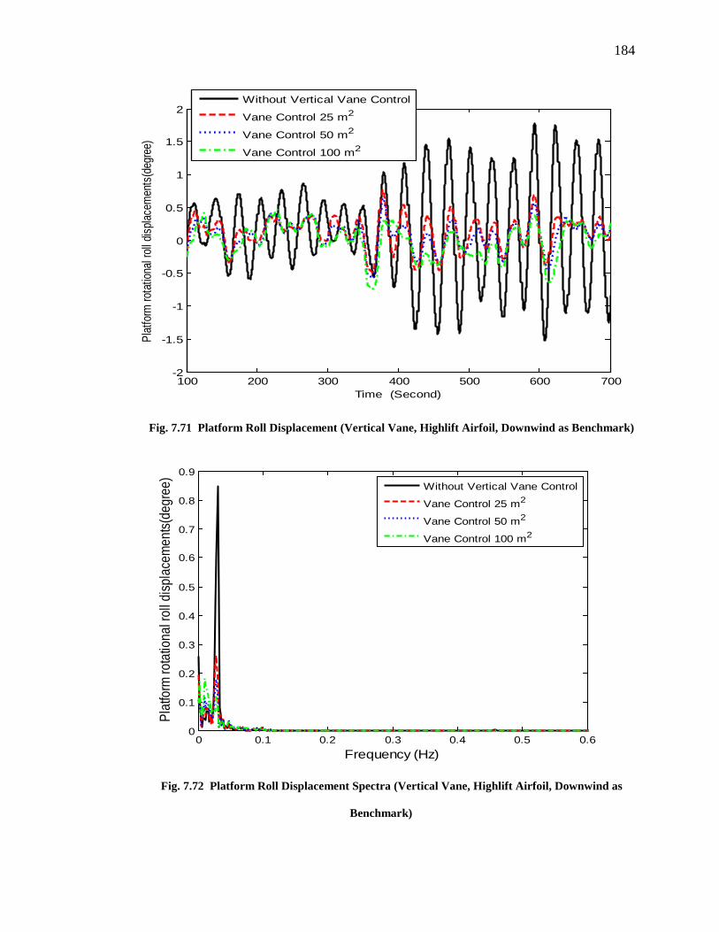
184
Fig. 7.71 Platform Roll Displacement (Vertical Vane, Highlift Airfoil, Downwind as Benchmark)
Fig. 7.72 Platform Roll Displacement Spectra (Vertical Vane, Highlift Airfoil, Downwind as
Benchmark)
100 200 300 400 500 600 700-2
-1.5
-1
-0.5
0
0.5
1
1.5
2
Time (Second)
Plat
form
rota
tiona
l roll
disp
lacem
ents
(deg
ree)
Without Vertical Vane Control
Vane Control 25 m2
Vane Control 50 m2
Vane Control 100 m2
0 0.1 0.2 0.3 0.4 0.5 0.60
0.1
0.2
0.3
0.4
0.5
0.6
0.7
0.8
0.9
Frequency (Hz)
Plat
form
rota
tiona
l rol
l disp
lace
men
ts(de
gree
)
Without Vertical Vane Control
Vane Control 25 m2
Vane Control 50 m2
Vane Control 100 m2

185
Fig. 7.73 Platform Sway Displacement (Vertical Vane, Highlift Airfoil, Downwind as
Benchmark)
Fig. 7.74 Platform Sway Displacement Spectra (Vertical Vane, Highlift Airfoil, Downwind as
Benchmark)
100 200 300 400 500 600 700-4
-3
-2
-1
0
1
2
3
Time (Second)
Plat
form
Tra
nslat
ional
Sway
Disp
lacem
ents
(m)
Without Vertical Vane Control
Vane Control 25 m2
Vane Control 50 m2
Vane Control 100 m2
0 0.1 0.2 0.3 0.4 0.5 0.60
0.2
0.4
0.6
0.8
1
1.2
1.4
Frequency (Hz)
Platf
orm
Tran
slatio
nal S
way D
isplac
emen
ts(m)
Without Vertical Vane Control
Vane Control 25 m2
Vane Control 50 m2
Vane Control 100 m2

186
Fig. 7.75 Side-to-Side Bending Moment (Vertical Vane, Highlift Airfoil, Downwind as
Benchmark)
Fig. 7.76 Side-to-Side Bending Moment Spectra (Vertical Vane, Highlift Airfoil, Downwind as
Benchmark)
100 200 300 400 500 600 700
-2
-1
0
1
2
3
4
x 104
Time (Second)
Side
-to-s
ide B
endin
g M
omen
ts a
t the
towe
r bas
e (k
N*m
)
Without Vertical Vane Control
Vane Control 25 m2
Vane Control 50 m2
Vane Control 100 m2
0 0.1 0.2 0.3 0.4 0.5 0.60
2000
4000
6000
8000
10000
12000
Frequency (Hz)Side
-to-si
de B
endin
g Mom
ents
at the
towe
r bas
e (kN
*m)
Without Vertical Vane Control
Vane Control 25 m2
Vane Control 50 m2
Vane Control 100 m2

187
7.3.1.6. Damage Equivalent Loads
When damping in roll direction of floating turbines is increased, loads at tower base in
side-to-side direction should be also reduced. In this section, the damage-equivalent loads
(DEL) of the moments at tower base in both side-to-side and fore-aft direction are
calculated by use of MCrunch [200] and results are listed in Table 7-3.
Table 7-3: Damage Equivalent Loads (DEL) for Vertical Vane
Cases Airfoil Vane Area
m2
Feedback Variable
Side-to-Side Moment at Tower Base
(kN*m)
Side-to-Side
Moment Reduction
Fore-Aft Moment at Tower Base
(kN*m)
Fore-Aft Moment
Reduction
1
(no vane)
---------- ---------- ---------- 23630.00 0.00% 68200 0.00%
2 NACA0012 25 Velocity 18560 21.46% 67330.00 1.28%
3 NACA0012 50 Velocity 16920 28.40% 67130.00 1.57%
4 NACA0012 100 Velocity 14920 36.86% 67440.00 1.11%
5 NACA0012 100 Acceleration 18730 20.74% 67440.00 1.11%
6 Highlift 25 Velocity 15910 32.67% 67370.00 1.23%
7 Highlift 50 Velocity 14470 38.76% 67540.00 0.97%
8 Highlift 100 Velocity 13410 43.25% 67970.00 0.34%
9 Highlift 100 Acceleration 14900 36.94% 67210.00 1.45%
7.3.1.7. Power Assumption by Vertical Vane Actuator
In this study, it is assumed that vane pitch angle is controlled by electrical motor. Vane
dynamics can be used to estimate torque and power which is needed for vane control.
Vane dynamics is shown in the below
m aeroJ T Tθ = − (7.1)

188
where θ is the pitch angle of vertical vane, J is the inertial moment of vertical vane and
Tm is electrical torque used for vane pitch control. Taero is the aerodynamic torque of
vertical vane according to the pitch axis located at 25% of the chord from the leading
edge of the airfoils in the cross-plane. Taero can be calculated by
( ) 212aero mT C v Aα ρ= ⋅ ⋅ (7.2)
where Cm is pitching moment coefficients of airfoils, α is angle of attack for vertical vane,
A is the vane area, ρ is air density and v is the mean wind speed for vane.
Torque from vane motor can be calculated by use of Eqs. (7.2) and (7.3). Then power
is used by vane motor can be estimated by use of the following formula
m mP T θ= ⋅ (7.3)
The power assumption of vane actuator and power production of wind turbine for
different cases are listed in Table 7-4.
Table 7-4: Power Assumption of Vane Pitch
Cases Airfoil Vane
Area m2
Feedback
Wind Turbine Power
Production (kWh)
Vane Actuator Power
Assumption (kWh)
Percent of Power
Assumption
1 Without Vane --------- ----------------- 1007 0 0.0000%
2 NACA0012 25 Velocity 1007.5 0.0551 0.0055%
3 NACA0012 50 Velocity 1007.3 0.1042 0.0103%
4 NACA0012 100 Velocity 1007 0.1678 0.0167%
5 NACA0012 100 Acceleration 1007.2 39.2684 3.8988%
Table 7-4 shows that:

189
a) When side-to-side velocity is used as measurement, the percentage of power
assumption ranges from 0.0055% to 0.0167% for vertical vane;
b) The bigger the vane area is, the higher the power assumption of vertical vane is;
c) Compared with that with velocity measurement, the power assumption of vertical
vane is higher (3.89%) when side-to-side acceleration at tower top is used as
measurement.
7.3.2. Simulation Results for Horizontal Vane
In this part, highlift airfoil and fore-aft velocity were proposed for horizontal vane control
based on experience of vertical vane control. Conditions of wind speed and wave are the
same to that for vertical vane control.
The vane pitch angle and its spectra are shown in Fig. 7.77 and Fig. 7.78. The fore-aft
velocity at tower top and its spectra are shown in Fig. 7.79 and Fig. 7.80. The rotational
pitch displacement and its spectra are shown in Fig. 7.81 and Fig. 7.82, which shows that
the variation of the platform pitch displacement was reduced about 40% near 0.02 Hz.
The fore-aft bending moment at the tower base and its spectra are plotted in Fig. 7.83 and
Fig. 7.84, which shows that variation of the fore-aft bending moment is reduced by about
50% near 0.02 Hz.

190
Fig. 7.77 Vane Pitch Angle for Horizontal Vane Control
Fig. 7.78 Vane Pitch Angle Spectra for Horizontal Vane Control
100 200 300 400 500 600 700-20
-15
-10
-5
0
5
10
15
20
25
Time (Second)
Vane
Pitc
h An
gle(d
egre
e)
Without Horizontal Vane ControlHorizontal Vane Control
0 0.1 0.2 0.3 0.4 0.5 0.60
2
4
6
8
10
12
14
Frequency (Hz)
Spec
tra o
f Van
e Pi
tch
Angl
e(de
gree
)
Without Horizontal Vane ControlHorizontal Vane Pitch Control

191
Fig. 7.79 Fore-aft Velocity at Tower Top for Horizontal Vane Control
Fig. 7.80. Spectra of Fore-aft Velocity at Tower Top for Horizontal Vane Control
100 200 300 400 500 600 700-3
-2
-1
0
1
2
3
Time (Second)
Fore
-aft
Velo
city
on
Towe
r Top
(m/s
)
Without Horizontal Vane ControlHorizontal Vane Control
0 0.1 0.2 0.3 0.4 0.5 0.60
0.1
0.2
0.3
0.4
0.5
0.6
0.7
Frequency (Hz)
Spec
tra o
f For
e-af
t Vel
ocity
on
Tow
er T
op(d
egre
e)
Without Horizontal Vane ControlHorizontal Vane Pitch Control

192
Fig. 7.81. Platform Rotational Pitch Displacement for Horizontal Vane Control
Fig. 7.82. Spectra of Platform Rotational Displacements for Horizontal Vane Control
100 200 300 400 500 600 700-2
-1
0
1
2
3
4
5
6
Time (Second)
Plat
form
rota
tiona
l pitc
h dis
place
men
ts(d
egre
e)
Without Horizontal Vane ControlHorizontal Vane Pitch Control
0 0.1 0.2 0.3 0.4 0.5 0.60
0.5
1
1.5
2
2.5
3
3.5
4
4.5
5
Frequency (Hz)Spec
tra o
f Pla
tform
rota
tiona
l pitc
h di
spla
cem
ents(
degr
ee)
Without Horizontal Vane ControlHorizontal Vane Pitch Control

193
Fig. 7.83. Fore-Aft Bending Moments at Tower Base for Horizontal Vane Control
Fig. 7.84. Spectra of Fore-Aft Bending Moments at Tower Base for Horizontal Vane Control
100 200 300 400 500 600 700-5
0
5
10
15x 10
4
Time (Second)
Fore
-aft
Bend
ing
Mom
ents
at t
he to
wer b
ase
(kN*
m)
Without Horizontal Vane ControlHorizontal Vane Pitch Control
0 0.1 0.2 0.3 0.4 0.5 0.60
1
2
3
4
5
6
7
8
9x 10
4
Frequency (Hz)
Spec
tra o
f For
e-af
t Ben
ding
Mom
ents
at t
he to
wer
bas
e (k
N*
Without Horizontal Vane ControlHorizontal Vane Pitch Control

194
7.4. Summary
In this chapter, a new actuator aerodynamics vane was proposed to increase damping of
floating wind turbine in the roll and pitch motion. The basic idea is to move wind turbine
back to balance line by use of aerodynamic forces of vertical vane when wind turbines
are not located in the balance line along the side-to-side direction. Tail-furling module of
FAST software is modified to simulate floating turbine including vanes. The benchmark
controller is built by use of PI-based individual pitch controller and variable torque
control. The PI-based vertical- and horizontal-vane controllers were designed by use of
both velocity and acceleration measurements at tower top. In order to evaluate the
capability of vertical vane, both airfoil NACA0012 and a highlift airfoil proposed in [35]
are used for vane design. Simulation results show that damping in the roll direction was
increased and side-to-side bending moments at tower was reduced from 19% to 42% by
use of vertical vane control and the power assumption for vertical vane control is not high.
For horizontal vane control, variation of platform pitch displacement was reduced about
40% and variation of fore-aft bending moment reduced about 50% at near 0.02 Hz.

195
Chapter 8. Contribution and Future Work
This dissertation research addresses several control problems for farm operated and
offshore floating turbines, covering both energy capture enhancement and load reduction.
As wind farm and offshore operations present the major engineering challenge and
opportunity for wind energy, this dissertation research has made more attempts on such
regard. This chapter concludes this dissertation by summarizing the major contributions
as well as suggesting some aspects of future work.
8.1. Summary of Research Contribution
8.1.1. Individual Pitch Control of Wind Turbine Load Reduction by
Including Wake Interaction
The Larsen wake model is chosen to compose the wind profile at the downstream wind
turbines under wake interaction, and a switched control strategy is thus developed based
on the composite wind profile. The idea of equivalent circular wind profile was proposed
to obtain different pitch references along azimuth. When different pitch references along
azimuth are used, more accurate state-space models of wind turbine can thus be generated
via FAST linearization. Based on such models, the IPC are designed following both the
DAC and the periodic control frameworks. Simulation results showed that the tower-base
fore-aft bending moment, the tower-base side-to-side bending moment, the rotor speed
fluctuation and the blade-tip displacement difference are significantly suppressed.

196
8.1.2. Model Predictive Control of Wind Turbines including Wake
Meandering
An MMPC based IPC design was presented for load reduction of wind turbine under a
wake meandering scenario. The spectral method with a special lateral coherence function
is used to generate the initial wind profile at the upstream wind turbine. Then a simplified
wake meandering model is used to predict the wake-center position at the downstream
wind turbine. Based on the wake center position thus calculated, the wind profile with
wake meandering was generated. After obtaining the linearized state-space models via
MBC, MMPC are designed in order to ensure smooth controller transition. Simulation
results showed that, compared that by use of traditional MPC, the variations in the rotor
speed and the blade-root flapwise moment are significantly suppressed by use of MMPC.
8.1.3. Maximizing Wind Farm Energy Capture via Nested-loop
Extremum Seeking Control
A nest-looped ESC controller is evaluated to maximize energy capture in wind farm level.
Based on analytical analysis and simulation, it is verified that optimal torque gains exists
and do not change with wind speed for maximizing energy capture in wind farm level.
For steady wind speed, power summation of all turbines in the wake of a turbine is used
as output measurement of this turbine’s ESC. For turbulent wind, power coefficients are
redefined in wind farm level and they are used for output measurement of ESC. Cross-
covariance is used to calculate the delay time of wake transportation. Simulation results
show that energy capture can be increased 5% under steady wind and 1.3% under
turbulent wind.

197
8.1.4. Active Vane Control for Stabilization of Floating Offshore Wind
Turbine
The active vane concept is evaluated for stabilization of floating wind turbine in both roll
and pitch motion. FAST software was modified to simulate floating turbine including
vane according to Kane’s method. The benchmark controller was built by use of PI-based
individual pitch controller and variable torque control. The PI-based vertical and
horizontal vane controllers were designed by use of both velocity and acceleration
measurements at tower top as feedback. In order to fully test the capability of vertical
vane, both airfoil NACA0012 and a highlift airfoil from Stanford were used for vane
design. Simulation results showed that side-to-side bending moments at tower was
reduced from 19% to 42% by use of the vertical vane control; the power assumption for
the vertical vane control is not high; damping of pitch motion for floating turbines was
increased by use of horizontal vane control.
8.2. Future Work
For MMPC control of wind turbine including wake meandering, MPC schemes of higher
robustness may be combined with MMPC framework in order to enhance stability
robustness. If the wake meandering situation can be formulated as a piece-wise affine
system, the hybrid MPC scheme can be applied.
The active vane design of higher lift can be investigated and the CFD study can be
performed. Coupling of vertical vane and horizontal vane will be a more interesting
research topic.
Experimental studies are necessary to further evaluate these above control strategies.

198
Appendix A. Justification of Nested-loop Optimization for
Maximizing Energy Capture of A Cascade of Wind Turbines
In this appendix, the optimal inductor factor relationship from [21, 22] is described
and the prove in this section was provided by Prof. Yaoyu Li. All the derivations are
based on the 1D Momentum Theory and the Actuator Disc Model of wind turbine. The
wind turbine array of interest is the cascaded topology as shown in Fig.A.1, where all the
wind turbine disks are lined up against the direction of the prevailing wind. For the ease
of the derivation later, the turbines are numbered along the upwind direction, i.e. turbine
1 is at the most the downwind position. For turbine i, Ui indicates its upcoming free-
stream wind speed. The row distance of the wind turbine array is designed such that the
free-stream average speed of the incoming wind for a downstream turbine can be
approximated as the far-wake average speed of an upstream turbine, i.e.
( )1 11 2i i iU a U+ += − (A.1)
where ai is the axial induction factor for the ith wind turbine.
Definition 1: Array Power Coefficient. For cascaded wind turbines 1, 2, …, n, … (as
illustrated in Fig.A.1 ), the Array Power Coefficient Kn for wind turbine n is defined as
( )1
31 2
n
jj
nn
PK
AUρ==∑
(A.2)

199
Fig. A.1 A Cascade of Wind Turbines
Lemma 1: For the cascaded wind turbine array as shown in Fig.A.1, when the total
power captured by the array is maximized, the optimal values of axial induction factors
of adjacent wind turbines, e.g. turbine n and turbine (n+1), are related by
**
1 *2 1n
nn
aaa+ =+
(A.3)
where the optimal induction factor of turbine n is
* 13 2( 1)na
n=
+ − (A.4)
Also, the array power coefficient of turbine n is
( )* *22 13n nK a= − (A.5)
Proof: To maximize the total power output of the wind turbine array in Fig.A.1, it is
equivalent to maximizing the array power coefficient for an arbitrary sub-array which
consists of turbines 1 to n, i.e.
Wind Direction
n n-1 n-2 2 1

200
( ) ( )3
31 11 13 1 2
1 2
n
jj n
n pn n pn n nn n
PUK C K C K a
AU Uρ= −
− −
= = + = + −
∑ (A.6)
where A is the rotor area and ρ is the air density, Un is the wind speed right in front of the
rotor of turbine n, and Cpn is the power coefficient of turbine n, i.e.
( )2
34 11
2
npn n n
n
PC a aAUρ
= = − (A.7)
Substitute Eq. (A.7) into (A.6) yields
( ) ( )2 314 1 1 2n n n n nK a a K a−= − + − (A.8)
To maximize Kn with respect to an, the first-order sufficient condition is
0n
n
dKda
= (A.9)
which leads to
( )( )( )1 2
2 1 1 31 2
n nn
n
a aK
a−
− −=
− (A.10)
Substituting Eq. (A.10) into Eq. (A.8) yields
( )* *22 13n nK a= − (A.11)
By extending Eq. (A.11) to Kn+1, the effective power efficient is

201
( )* * 21 1
2 13n nK a− −= − (A.12)
Then, substituting Eqs. (A.11) and (A.12) into Eq. (A.8) yields
** 1
*12 1
nn
n
aaa
−
−
=+
(A.13)
Based on Eq. (A.10), we can derive
* 13 2( 1)na
n=
+ − (A.14)
Proposition 1: For a cascaded wind turbine array in Fig.A.1 , the optimal axial induction
factors of turbine n ≥ 2 follows
* 10, 3na ∈ (A.15)
Proof: from Eq. (A.4) in Lemma 1, the optimal axial induction factor for turbines 1, 2,
3,… , respectively, form a positive and decreasing series 1/3, 1/5, 1/7, …, which results
in Eq. (A.6).
Proposition 2: For a cascaded wind turbine array in Fig.A.1, the optimal array power
coefficient of turbine n ≥ 1 is
* 16 2,27 3nK ∈ (A.16)
Proof: Substituting Eq. (A.6) into Eq. (A.5) yields Eq. (A.16).

202
Theorem 1: For cascaded wind turbine array as shown in Fig.A.1, the maximum total
power of n+1 turbines (n ≥ 1) can be uniquely optimized by optimizing the axial
induction factor of the most upwind turbine (i.e. an+1) and optimizing the array power
coefficient of the immediate downwind turbine Kn (i.e. the total power of all downwind
turbines).
Proof: For turbine n and (n+1), we have
( )1 11 2n n nU a U+ += −
1. The array power coefficient for turbine (n+1) is
( ) ( ) ( )
1
3
1 1 11 , 13 3 3
1 1 1 11 2 1 2 1 2
n n
i ii n i n
n P n nn n n n
P PP UK C K
AU AU AU Uρ ρ ρ
+
= + =+ +
+ + + +
= = + = +
∑ ∑
Therefore, we have
( ) ( )2 31 1 1 14 1 1 2n n n n nK a a K a+ + + += − + − (A.17)
Maximizing Kn+1 relies on both an+1 and Kn. As Kn is function of dimensionless numbers
a1, …, an, Kn(a1, …, an) is invariant with Un+1,and in consequence independent on an+1.
Since an+1∈(0, ½), 4an+1(1− an+1)2>0, and (1−2an+1)3 >0. Also, Kn > 0, we have Kn+1 > 0
from Eq. (15). From Eq. (A.16), the limit of Kn is 2/3, so Kn+1(an+1, Kn) is positive-value
function defined on a Cartesian domain (0, ½)×[16/27,2/3]. An important implication for
wind turbine array optimization is that, once the operational parameters of a sub-array of
wind turbines is optimized (by adjusting the axial induction factors of the involved
turbines), adjustment of upwind turbines would not affect such optimality.

203
2. For any fixed an+1, attaining the maximum for Kn+1 (i.e. *1nK + ) will require Kn
achieves its maximum, i.e. Kn,max. An easy proof by contradiction can be set as follows.
If the pair ( )* *1,n na K+ maximized Kn+1, where *
,maxn nK K< , we would have
( ) ( ) ( ) ( )2 3 2 3* * * * * * *1 1 1 1 1 ,max 14 1 1 2 4 1 1 2+ + + + + +− + − < − + −n n n n n n n na a K a a a K a
which results in *,maxn nK K= .
An important implication of this statement is that the optimal choice of Kn regarding to
optimizing Kn+1 is fixed to Kn,max, which is result of maximizing the total power of all
downwind turbines. In other words, it shows a “common-sense” consequence – the total
power of (n+1) turbines would be maximized after the total power of the n downwind
turbines is optimized.
3. Then the task of maximizing Kn+1 in Eq. (15) can be simplified as
( ) ( )1
2 3*1 1 1 1arg max 4 1 1 2
nn n n n na
K a a K a+
+ + + + = − + − (A.18)
where Kn can be considered as a constant for this optimization problem, which can reach
its maximum Kn,max by adjusting (a1, …, an) in a separate problem. For all the following
derivation, the axial inductor factor has permissible range of
( )1 0,1 2na + ∈
Consider the first-order sufficient condition for optimality,
1
1
0n
n
dKda
+
+
= (A.19)

204
Since
( ) ( ) ( )211 1
1
12 24 24 16 4 6nn n n n n
n
dK K a K a Kda
++ +
+
= − + − + − (A.20)
Eq. (A.19) becomes
( ) ( ) ( )( )
( )
21 1
1
6 12 12 8 2 3 0
8 12 16 242 6 12
n n n n n
n nn
n
K a K a K
K Ka
K
+ +
+
− + − + − =
− ± −⇒ =
−
This results in
( )( )1
4 6 4 66 12
n nn
n
K Ka
K+
− ± −=
− (A.21)
Due to the possible singularity in the denominator in Eq.(A.21) and also different
possible solutions, we need to separate three cases:
i) ( ) ( ) ( ) ( )1 2, : 6 12 0, 4 6 0,1 4 6 4 62 3n n n n nK K and K K K ∈ − < − ∈ ⇒ − > −
( )( )1
4 6 4 66 12
n nn
n
K Ka
K+
− − −⇒ =
− is the only positive solution.
This is the situation when the total power of all the downwind turbines have been
optimized, the axial inductor factor of the current turbine can be optimized to a
unique solution.
ii) For Kn=1/2:

205
( ) ( ) ( )21 1 1
112 24 24 16 4 6 04n n n n n nK a K a K a+ + +− + − + − = ⇒ =
iii) 10, :2nK ∈
( ) ( ) ( ) ( )6 12 0, 4 6 1, 4 4 6 4 6n n n nK and K K K− > − ∈ ⇒ − < −
( )( )1
4 6 4 66 12+
− ± −⇒ =
−n n
nn
K Ka
K are two positive real roots.
Now we will test if both roots lie in the permissible range of (0, ½) for axial
induction factor.
( )( ) ( ) ( )1
4 6 4 6 4 61 1 16 12 6 1 2 2 6 1 2 2
n n nn
n n n
K K Ka
K K K+
− + − −= = + + >
− − −
This is an impossible solution.
Therefore, only ( )
( )1
4 6 4 66 12
n nn
n
K Ka
K+
− − −=
− is the possible solution, which is the
same as the case i).
4. To show the existence of unique an+1, we need to verify the following second-
order derivative condition to validate an obtained stationary point as maximum:
21
21
0n
n
d Kda
+
+
< (A.22)
( ) ( )2
112
1
2 6 12 12 8nn n n
n
d K K a Kda
++
+
= − + − (A.23)

206
i) For Kn=1/2, 2
12
1
2n
n
d Kda
+
+
= − , i.e. 2
12
1
0+
+
<n
n
d Kda
for all an+1.
ii) Otherwise Kn+1 ≠ ½, substituting the aforementioned root (for cases i and iii in the
part 3) into Eq. (A.23) yields
( )( )1
4 6 4 66 12
n nn
n
K Ka
K+
− − −=
− ,
21
21
4 6 0nn
n
d K Kda
+
+
= − − < and 2
12
1
0n
n
d Kda
+
+
< since Kn < 2/3.
Combining both case yields that therefore there exist interior point of an+1 that is
unique optimal solution.

207
Appendix B. Specifications of NREL 5MW Turbine Model
In this appendix, main characteristics of NREL 5MW [192] is provided in Table B-1.
Table B-1: Properties of the NREL-5MW Baseline
Rated Power 5 MW
Rotor Orientation Upwind
Blade number 3 Blades
Rotor, Hub Diameter 126m, 3m
Rotor Mass 110,000 kg
Nacelle Mass 240,000kg
Tower Mass 347,460kg
Rated Tip Speed 80 m/s
Cut-In, Rated Rotor Speed 6.9rpm, 12.1rpm
Cut-In, Rated, Cut-out Wind Speeds 3m/s, 11.4m/s, 25m/s
Gearbox Ratio 97
Generator Efficiency 94.4%
For more detailed description for the characteristics of the NREL 5MW turbine model,
the FAST [140] input file is copied as follows:
-------------------------------------------------------------------------------- ------- FAST INPUT FILE -------------------------------------------------------- NREL 5.0 MW Baseline Wind Turbine for Use in Offshore Analysis. Properties from Dutch Offshore Wind Energy Converter (DOWEC) 6MW Pre-Design (10046_009.pdf) and REpower 5M 5MW (5m_uk.pdf); Compatible with FAST v6.0. ---------------------- SIMULATION CONTROL -------------------------------------- False Echo - Echo input data to "echo.out" (flag) 1 ADAMSPrep - ADAMS preprocessor mode 1: Run FAST, 2: use FAST as a preprocessor to create an ADAMS model, 3: do both (switch)

208
1 AnalMode - Analysis mode 1: Run a time-marching simulation, 2: create a periodic linearized model (switch) 3 NumBl - Number of blades (-) 630.0 TMax - Total run time (s) 0.0125 DT - Integration time step (s) ---------------------- TURBINE CONTROL ----------------------------------------- 0 YCMode - Yaw control mode 0: none, 1: user-defined from routine UserYawCont, 2: user-defined from Simulink (switch) 9999.9 TYCOn - Time to enable active yaw control (s) [unused when YCMode=0] 2 PCMode - Pitch control mode 0: none, 1: user-defined from routine PitchCntrl, 2: user-defined from Simulink (switch) 0.0 TPCOn - Time to enable active pitch control (s) [unused when PCMode=0] 3 VSContrl - Variable-speed control mode 0: none, 1: simple VS, 2: user-defined from routine UserVSCont, 3: user-defined from Simulink (switch) 1173.7 VS_RtGnSp - Rated generator speed for simple variable-speed generator control (HSS side) (rpm) [used only when VSContrl=1] 43093.55 VS_RtTq - Rated generator torque/constant generator torque in Region 3 for simple variable-speed generator control (HSS side) (N-m) [used only when VSContrl=1] 0.0255764 VS_Rgn2K - Generator torque constant in Region 2 for simple variable-speed generator control (HSS side) (N-m/rpm^2) [used only when VSContrl=1] 10.0 VS_SlPc - Rated generator slip percentage in Region 2 1/2 for simple variable-speed generator control (%) [used only when VSContrl=1] 1 GenModel - Generator model 1: simple, 2: Thevenin, 3: user-defined from routine UserGen (switch) [used only when VSContrl=0] True GenTiStr - Method to start the generator T: timed using TimGenOn, F: generator speed using SpdGenOn (flag) True GenTiStp - Method to stop the generator T: timed using TimGenOf, F: when generator power = 0 (flag) 9999.9 SpdGenOn - Generator speed to turn on the generator for a startup (HSS speed) (rpm) [used only when GenTiStr=False] 0.0 TimGenOn - Time to turn on the generator for a startup (s) [used only when GenTiStr=True] 9999.9 TimGenOf - Time to turn off the generator (s) [used only when GenTiStp=True] 1 HSSBrMode - HSS brake model 1: simple, 2: user-defined from routine UserHSSBr (switch) 9999.9 THSSBrDp - Time to initiate deployment of the HSS brake (s) 9999.9 TiDynBrk - Time to initiate deployment of the dynamic generator brake [CURRENTLY IGNORED] (s) 9999.9 TTpBrDp(1) - Time to initiate deployment of tip brake 1 (s) 9999.9 TTpBrDp(2) - Time to initiate deployment of tip brake 2 (s) 9999.9 TTpBrDp(3) - Time to initiate deployment of tip brake 3 (s) [unused for 2 blades] 9999.9 TBDepISp(1) - Deployment-initiation speed for the tip brake on blade 1 (rpm) 9999.9 TBDepISp(2) - Deployment-initiation speed for the tip brake on blade 2 (rpm) 9999.9 TBDepISp(3) - Deployment-initiation speed for the tip brake on blade 3 (rpm) [unused for 2 blades] 9999.9 TYawManS - Time to start override yaw maneuver and end standard yaw control (s) 9999.9 TYawManE - Time at which override yaw maneuver reaches final yaw angle (s) 0.0 NacYawF - Final yaw angle for yaw maneuvers (degrees) 9999.9 TPitManS(1) - Time to start override pitch maneuver for blade 1 and end standard pitch control (s) 9999.9 TPitManS(2) - Time to start override pitch maneuver for blade 2 and end standard pitch control (s) 9999.9 TPitManS(3) - Time to start override pitch maneuver for blade 3 and end standard pitch control (s) [unused for 2 blades] 9999.9 TPitManE(1) - Time at which override pitch maneuver for blade 1 reaches final pitch (s) 9999.9 TPitManE(2) - Time at which override pitch maneuver for blade 2 reaches final pitch (s) 9999.9 TPitManE(3) - Time at which override pitch maneuver for blade 3 reaches final pitch (s) [unused for 2 blades]

209
14.749 BlPitch(1) - Blade 1 initial pitch (degrees) 14.749 BlPitch(2) - Blade 2 initial pitch (degrees) 14.749 BlPitch(3) - Blade 3 initial pitch (degrees) [unused for 2 blades] 0.0 B1PitchF(1) - Blade 1 final pitch for pitch maneuvers (degrees) 0.0 B1PitchF(2) - Blade 2 final pitch for pitch maneuvers (degrees) 0.0 B1PitchF(3) - Blade 3 final pitch for pitch maneuvers (degrees) [unused for 2 blades] ---------------------- ENVIRONMENTAL CONDITIONS -------------------------------- 9.80665 Gravity - Gravitational acceleration (m/s^2) ---------------------- FEATURE FLAGS ------------------------------------------- True FlapDOF1 - First flapwise blade mode DOF (flag) False FlapDOF2 - Second flapwise blade mode DOF (flag) False EdgeDOF - First edgewise blade mode DOF (flag) False TeetDOF - Rotor-teeter DOF (flag) [unused for 3 blades] True DrTrDOF - Drivetrain rotational-flexibility DOF (flag) True GenDOF - Generator DOF (flag) False YawDOF - Yaw DOF (flag) True TwFADOF1 - First fore-aft tower bending-mode DOF (flag) False TwFADOF2 - Second fore-aft tower bending-mode DOF (flag) True TwSSDOF1 - First side-to-side tower bending-mode DOF (flag) False TwSSDOF2 - Second side-to-side tower bending-mode DOF (flag) True CompAero - Compute aerodynamic forces (flag) False CompNoise - Compute aerodynamic noise (flag) ---------------------- INITIAL CONDITIONS -------------------------------------- 0.0 OoPDefl - Initial out-of-plane blade-tip displacement (meters) 0.0 IPDefl - Initial in-plane blade-tip deflection (meters) 0.0 TeetDefl - Initial or fixed teeter angle (degrees) [unused for 3 blades] 0.0 Azimuth - Initial azimuth angle for blade 1 (degrees) 12.1 RotSpeed - Initial or fixed rotor speed (rpm) 0.0 NacYaw - Initial or fixed nacelle-yaw angle (degrees) 0.0 TTDspFA - Initial fore-aft tower-top displacement (meters) 0.0 TTDspSS - Initial side-to-side tower-top displacement (meters) ---------------------- TURBINE CONFIGURATION ----------------------------------- 63.0 TipRad - The distance from the rotor apex to the blade tip (meters) 1.5 HubRad - The distance from the rotor apex to the blade root (meters) 1 PSpnElN - Number of the innermost blade element which is still part of the pitchable portion of the blade for partial-span pitch control [1 to BldNodes] [CURRENTLY IGNORED] (-) 0.0 UndSling - Undersling length [distance from teeter pin to the rotor apex] (meters) [unused for 3 blades] 0.0 HubCM - Distance from rotor apex to hub mass [positive downwind] (meters) -5.01910 OverHang - Distance from yaw axis to rotor apex [3 blades] or teeter pin [2 blades] (meters) 1.9 NacCMxn - Downwind distance from the tower-top to the nacelle CM (meters) 0.0 NacCMyn - Lateral distance from the tower-top to the nacelle CM (meters) 1.75 NacCMzn - Vertical distance from the tower-top to the nacelle CM (meters) 87.6 TowerHt - Height of tower above ground level [onshore] or MSL [offshore] (meters) 1.96256 Twr2Shft - Vertical distance from the tower-top to the rotor shaft (meters) 0.0 TwrRBHt - Tower rigid base height (meters) -5.0 ShftTilt - Rotor shaft tilt angle (degrees) 0.0 Delta3 - Delta-3 angle for teetering rotors (degrees) [unused for 3 blades] -2.5 PreCone(1) - Blade 1 cone angle (degrees) -2.5 PreCone(2) - Blade 2 cone angle (degrees) -2.5 PreCone(3) - Blade 3 cone angle (degrees) [unused for 2 blades] 0.0 AzimB1Up - Azimuth value to use for I/O when blade 1 points up (degrees) ---------------------- MASS AND INERTIA ---------------------------------------- 0.0 YawBrMass - Yaw bearing mass (kg) 240.00E3 NacMass - Nacelle mass (kg) 56.78E3 HubMass - Hub mass (kg)
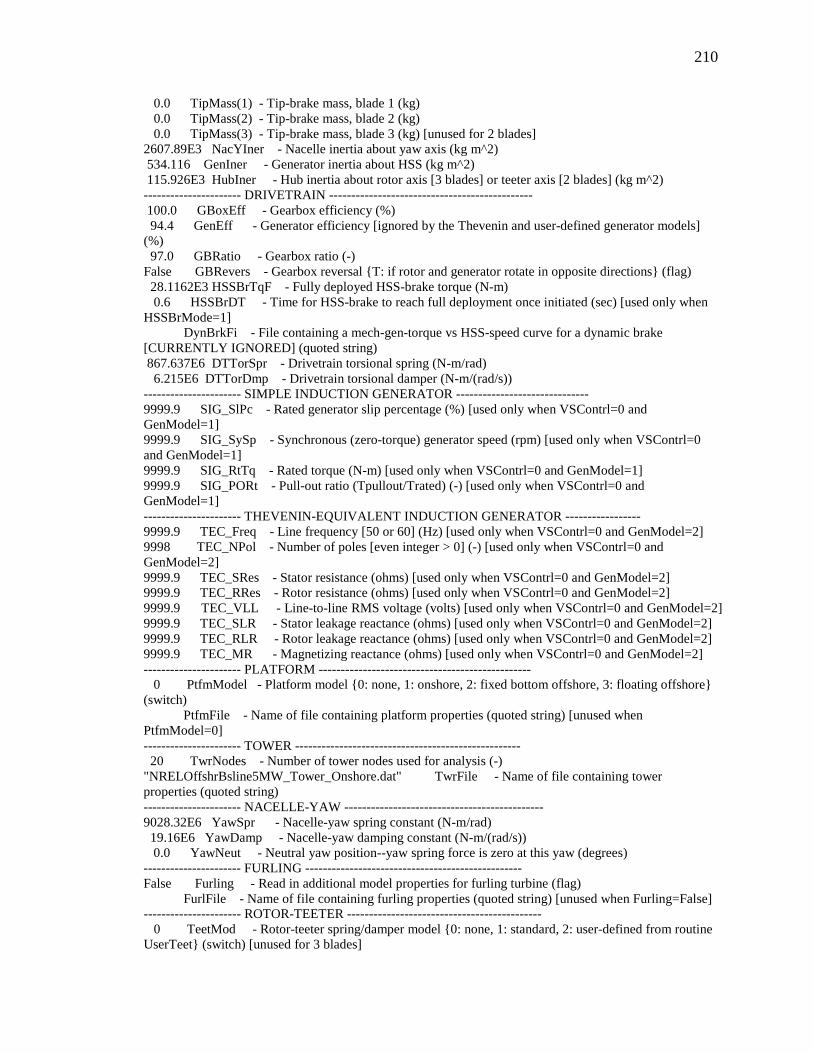
210
0.0 TipMass(1) - Tip-brake mass, blade 1 (kg) 0.0 TipMass(2) - Tip-brake mass, blade 2 (kg) 0.0 TipMass(3) - Tip-brake mass, blade 3 (kg) [unused for 2 blades] 2607.89E3 NacYIner - Nacelle inertia about yaw axis (kg m^2) 534.116 GenIner - Generator inertia about HSS (kg m^2) 115.926E3 HubIner - Hub inertia about rotor axis [3 blades] or teeter axis [2 blades] (kg m^2) ---------------------- DRIVETRAIN ---------------------------------------------- 100.0 GBoxEff - Gearbox efficiency (%) 94.4 GenEff - Generator efficiency [ignored by the Thevenin and user-defined generator models] (%) 97.0 GBRatio - Gearbox ratio (-) False GBRevers - Gearbox reversal T: if rotor and generator rotate in opposite directions (flag) 28.1162E3 HSSBrTqF - Fully deployed HSS-brake torque (N-m) 0.6 HSSBrDT - Time for HSS-brake to reach full deployment once initiated (sec) [used only when HSSBrMode=1] DynBrkFi - File containing a mech-gen-torque vs HSS-speed curve for a dynamic brake [CURRENTLY IGNORED] (quoted string) 867.637E6 DTTorSpr - Drivetrain torsional spring (N-m/rad) 6.215E6 DTTorDmp - Drivetrain torsional damper (N-m/(rad/s)) ---------------------- SIMPLE INDUCTION GENERATOR ------------------------------ 9999.9 SIG_SlPc - Rated generator slip percentage (%) [used only when VSContrl=0 and GenModel=1] 9999.9 SIG_SySp - Synchronous (zero-torque) generator speed (rpm) [used only when VSContrl=0 and GenModel=1] 9999.9 SIG_RtTq - Rated torque (N-m) [used only when VSContrl=0 and GenModel=1] 9999.9 SIG_PORt - Pull-out ratio (Tpullout/Trated) (-) [used only when VSContrl=0 and GenModel=1] ---------------------- THEVENIN-EQUIVALENT INDUCTION GENERATOR ----------------- 9999.9 TEC_Freq - Line frequency [50 or 60] (Hz) [used only when VSContrl=0 and GenModel=2] 9998 TEC_NPol - Number of poles [even integer > 0] (-) [used only when VSContrl=0 and GenModel=2] 9999.9 TEC_SRes - Stator resistance (ohms) [used only when VSContrl=0 and GenModel=2] 9999.9 TEC_RRes - Rotor resistance (ohms) [used only when VSContrl=0 and GenModel=2] 9999.9 TEC_VLL - Line-to-line RMS voltage (volts) [used only when VSContrl=0 and GenModel=2] 9999.9 TEC_SLR - Stator leakage reactance (ohms) [used only when VSContrl=0 and GenModel=2] 9999.9 TEC_RLR - Rotor leakage reactance (ohms) [used only when VSContrl=0 and GenModel=2] 9999.9 TEC_MR - Magnetizing reactance (ohms) [used only when VSContrl=0 and GenModel=2] ---------------------- PLATFORM ------------------------------------------------ 0 PtfmModel - Platform model 0: none, 1: onshore, 2: fixed bottom offshore, 3: floating offshore (switch) PtfmFile - Name of file containing platform properties (quoted string) [unused when PtfmModel=0] ---------------------- TOWER --------------------------------------------------- 20 TwrNodes - Number of tower nodes used for analysis (-) "NRELOffshrBsline5MW_Tower_Onshore.dat" TwrFile - Name of file containing tower properties (quoted string) ---------------------- NACELLE-YAW --------------------------------------------- 9028.32E6 YawSpr - Nacelle-yaw spring constant (N-m/rad) 19.16E6 YawDamp - Nacelle-yaw damping constant (N-m/(rad/s)) 0.0 YawNeut - Neutral yaw position--yaw spring force is zero at this yaw (degrees) ---------------------- FURLING ------------------------------------------------- False Furling - Read in additional model properties for furling turbine (flag) FurlFile - Name of file containing furling properties (quoted string) [unused when Furling=False] ---------------------- ROTOR-TEETER -------------------------------------------- 0 TeetMod - Rotor-teeter spring/damper model 0: none, 1: standard, 2: user-defined from routine UserTeet (switch) [unused for 3 blades]

211
0.0 TeetDmpP - Rotor-teeter damper position (degrees) [used only for 2 blades and when TeetMod=1] 0.0 TeetDmp - Rotor-teeter damping constant (N-m/(rad/s)) [used only for 2 blades and when TeetMod=1] 0.0 TeetCDmp - Rotor-teeter rate-independent Coulomb-damping moment (N-m) [used only for 2 blades and when TeetMod=1] 0.0 TeetSStP - Rotor-teeter soft-stop position (degrees) [used only for 2 blades and when TeetMod=1] 0.0 TeetHStP - Rotor-teeter hard-stop position (degrees) [used only for 2 blades and when TeetMod=1] 0.0 TeetSSSp - Rotor-teeter soft-stop linear-spring constant (N-m/rad) [used only for 2 blades and when TeetMod=1] 0.0 TeetHSSp - Rotor-teeter hard-stop linear-spring constant (N-m/rad) [used only for 2 blades and when TeetMod=1] ---------------------- TIP-BRAKE ----------------------------------------------- 0.0 TBDrConN - Tip-brake drag constant during normal operation, Cd*Area (m^2) 0.0 TBDrConD - Tip-brake drag constant during fully-deployed operation, Cd*Area (m^2) 0.0 TpBrDT - Time for tip-brake to reach full deployment once released (sec) ---------------------- BLADE --------------------------------------------------- "NRELOffshrBsline5MW_Blade.dat" BldFile(1) - Name of file containing properties for blade 1 (quoted string) "NRELOffshrBsline5MW_Blade.dat" BldFile(2) - Name of file containing properties for blade 2 (quoted string) "NRELOffshrBsline5MW_Blade.dat" BldFile(3) - Name of file containing properties for blade 3 (quoted string) [unused for 2 blades] ---------------------- AERODYN ------------------------------------------------- "NRELOffshrBsline5MW_AeroDyn_WM.ipt" ADFile - Name of file containing AeroDyn input parameters (quoted string) ---------------------- NOISE --------------------------------------------------- NoiseFile - Name of file containing aerodynamic noise input parameters (quoted string) [used only when CompNoise=True] ---------------------- ADAMS --------------------------------------------------- "NRELOffshrBsline5MW_ADAMSSpecific.dat" ADAMSFile - Name of file containing ADAMS-specific input parameters (quoted string) [unused when ADAMSPrep=1] ---------------------- LINEARIZATION CONTROL ----------------------------------- "NRELOffshrBsline5MW_Linear.dat" LinFile - Name of file containing FAST linearization parameters (quoted string) [unused when AnalMode=1] ---------------------- OUTPUT -------------------------------------------------- True SumPrint - Print summary data to "<RootName>.fsm" (flag) True TabDelim - Generate a tab-delimited tabular output file. (flag) "ES10.3E2" OutFmt - Format used for tabular output except time. Resulting field should be 10 characters. (quoted string) [not checked for validity!] 0.0 TStart - Time to begin tabular output (s) 1 DecFact - Decimation factor for tabular output 1: output every time step (-) 1.0 SttsTime - Amount of time between screen status messages (sec) -3.09528 NcIMUxn - Downwind distance from the tower-top to the nacelle IMU (meters) 0.0 NcIMUyn - Lateral distance from the tower-top to the nacelle IMU (meters) 2.23336 NcIMUzn - Vertical distance from the tower-top to the nacelle IMU (meters) 1.912 ShftGagL - Distance from rotor apex [3 blades] or teeter pin [2 blades] to shaft strain gages [positive for upwind rotors] (meters) 0 NTwGages - Number of tower nodes that have strain gages for output [0 to 9] (-) TwrGagNd - List of tower nodes that have strain gages [1 to TwrNodes] (-) [unused if NTwGages=0] 3 NBlGages - Number of blade nodes that have strain gages for output [0 to 9] (-) 5,9,13 BldGagNd - List of blade nodes that have strain gages [1 to BldNodes] (-) [unused if NBlGages=0]

212
OutList - The next line(s) contains a list of output parameters. See OutList.txt for a listing of available output channels, (-) "WindVxi , WindVyi , WindVzi" - Longitudinal, lateral, and vertical wind speeds "GenPwr , GenTq" - Electrical generator power and torque "OoPDefl1 , IPDefl1 , TwstDefl1" - Blade 1 out-of-plane and in-plane deflections and tip twist "BldPitch1" - Blade 1 pitch angle "BldPitch2" - Blade 2 pitch angle "BldPitch3" - Blade 3 pitch angle "Azimuth" - Blade 1 azimuth angle "RotSpeed , GenSpeed" - Low-speed shaft and high-speed shaft speeds "TTDspFA , TTDspSS , TTDspTwst" - Tower fore-aft and side-to-side displacments and top twist "Spn2MLxb1, Spn2MLyb1" - Blade 1 local edgewise and flapwise bending moments at span station 2 (approx. 50% span) "RootFxc1 , RootFyc1 , RootFzc1" - Out-of-plane shear, in-plane shear, and axial forces at the root of blade 1 "RootMxc1 , RootMyc1 , RootMzc1" - In-plane bending, out-of-plane bending, and pitching moments at the root of blade 1 "RootMxc2 , RootMyc2 , RootMzc2" "RootMxc3 , RootMyc3 , RootMzc3" "RootMyb1" - flapwise moment at the root of blade 1 "RootMyb2" - flapwise moment at the root of blade 2 "RootMyb3" - flapwise moment at the root of blade 3 "RotTorq , LSSGagMya, LSSGagMza" - Rotor torque and low-speed shaft 0- and 90-bending moments at the main bearing "YawBrFxp , YawBrFyp , YawBrFzp" - Fore-aft shear, side-to-side shear, and vertical forces at the top of the tower (not rotating with nacelle yaw) "YawBrMxp , YawBrMyp , YawBrMzp" - Side-to-side bending, fore-aft bending, and yaw moments at the top of the tower (not rotating with nacelle yaw) "TwrBsFxt , TwrBsFyt , TwrBsFzt" - Fore-aft shear, side-to-side shear, and vertical forces at the base of the tower (mudline) "TwrBsMxt , TwrBsMyt , TwrBsMzt" - Side-to-side bending, fore-aft bending, and yaw moments at the base of the tower (mudline) "rotcq" "rotpwr" "YawBrTDxt" - Tower-top/yaw bearing fore-aft (translational) deflection "YawBrTDyt" - Tower-top/yaw bearing fore-aft (translational) deflection "TipDxc1,TipDxc2,TipDxc3" - Blade 1, 2, 3 out-of-plane tip deflection (relative to the pitch axis) END of FAST input file (the word "END" must appear in the first 3 columns of this last line). --------------------------------------------------------------------------------

213
Appendix C. Codes of MMPC and dual-mode MPC
C.1 Multiple Model Predictive Control
C.1.1 Source Codes
function [c1,c2,c3]=mmmpc(Weighting,SwS,Est11,Est12,Est13,Est14,Est15,Est16,Est17,Est21,Est22,Est23,Est24,Est25,Est26,Est27,phi,omega,Wy,Wu,A,B,C,PitchRef,pinvM) %#eml eml.extrinsic('qpOASES'); % eml.extrinsic('pinv'); Ts=0.1; % Decide model number if SwS-round(SwS)>=0.0 k=round(SwS)+1; else k=round(SwS)+1-1; end % Calculate pitch reference if k>=11 ur=PitchRef(11)*180/pi; else ur=Weighting*PitchRef(k)*180/pi+(1-Weighting)*PitchRef(k+1)*180/pi; % PitchRefW=pi*PitchRefW/180; end

214
if k<=0 k=1; end if k>11 k=11; end % Set parameters for MPC design nc=20; p=nc; m=p; nu=3; ny=4; % uc=[p1;p2;p3]; U0=zeros(nu*m,1); % Extract two models from the model bank [Cn,Cm,Cll]=size(C); CC1=zeros(Cn,Cm); CC2=zeros(Cn,Cm); [Bn,Bm,Bll]=size(B); BB1=zeros(Bn,Bm); BB2=zeros(Bn,Bm); [An,Am,All]=size(A); AA1=zeros(An,Am); AA2=zeros(An,Am); % for nn=1:Cn % for mm=1:Cm % C1(nn,mm)=C(nn,mm,1); % end % end if k<11

215
for nn=1:Cn for mm=1:Cm CC1(nn,mm)=C(nn,mm,k); CC2(nn,mm)=C(nn,mm,k+1); end end for nn=1:Bn for mm=1:Bm BB1(nn,mm)=B(nn,mm,k); BB2(nn,mm)=B(nn,mm,k+1); end end for nn=1:An for mm=1:Am AA1(nn,mm)=A(nn,mm,k); AA2(nn,mm)=A(nn,mm,k+1); end end else LL=10; for nn=1:Cn for mm=1:Cm CC1(nn,mm)=C(nn,mm,LL); CC2(nn,mm)=C(nn,mm,LL+1); end end for nn=1:Bn for mm=1:Bm BB1(nn,mm)=B(nn,mm,LL); BB2(nn,mm)=B(nn,mm,LL+1); end end for nn=1:An for mm=1:Am AA1(nn,mm)=A(nn,mm,LL); AA2(nn,mm)=A(nn,mm,LL+1); end end

216
end [An,Am]=size(AA1); [Bn,Bm]=size(BB1); ModL=2; xhat1=[Est11;Est12;Est13;Est14;Est15;Est16;Est17;]; xhat2=[Est21;Est22;Est23;Est24;Est25;Est26;Est27;]; %% Formulate the matrix in quadratic programming % generate Sx Sx=zeros(ny*p,1); for nn=1:ModL if nn==1 Cnn=CC1; Ann=AA1; xhat=xhat1; Weightnn=Weighting; else Cnn=CC2; Ann=AA2; xhat=xhat2; Weightnn=1-Weighting; end Sx_temp=zeros(ny*p,Am); for ii=1:p Sx_temp_part=Cnn*Ann^(ii); for jj=1:ny for kk=1:Am Sx_temp(ny*(ii-1)+jj,kk)=Sx_temp_part(jj,kk); end end end Sx=Sx+Weightnn*Sx_temp*xhat; end
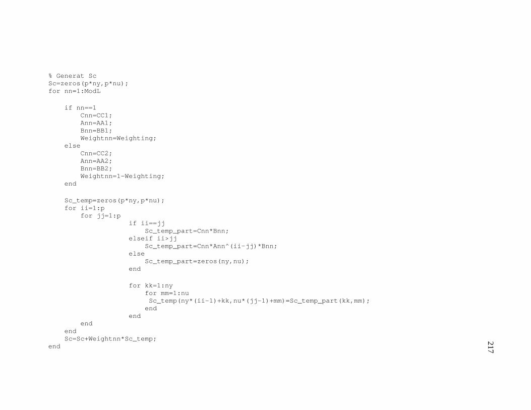
217
% Generat Sc Sc=zeros(p*ny,p*nu); for nn=1:ModL if nn==1 Cnn=CC1; Ann=AA1; Bnn=BB1; Weightnn=Weighting; else Cnn=CC2; Ann=AA2; Bnn=BB2; Weightnn=1-Weighting; end Sc_temp=zeros(p*ny,p*nu); for ii=1:p for jj=1:p if ii==jj Sc_temp_part=Cnn*Bnn; elseif ii>jj Sc_temp_part=Cnn*Ann^(ii-jj)*Bnn; else Sc_temp_part=zeros(ny,nu); end for kk=1:ny for mm=1:nu Sc_temp(ny*(ii-1)+kk,nu*(jj-1)+mm)=Sc_temp_part(kk,mm); end end end end Sc=Sc+Weightnn*Sc_temp; end
218
% Generate Se Se=zeros(p*nu,m*nu); for ii=1:p for jj=1:m if ii==jj for kk=1:nu for mm=1:nu if kk==mm Se(nu*(ii-1)+kk,nu*(jj-1)+mm)=1.0; else Se(nu*(ii-1)+kk,nu*(jj-1)+mm)=0.0; end end end elseif ii>jj for kk=1:nu for mm=1:nu if kk==mm Se(nu*(ii-1)+kk,nu*(jj-1)+mm)=1.0; else Se(nu*(ii-1)+kk,nu*(jj-1)+mm)=0.0; end end end elseif ii<jj for kk=1:nu for mm=1:nu Se(nu*(ii-1)+kk,nu*(jj-1)+mm)=0.0; end end end end end % U0=zeros(nu*m,1); H=2*Wu+2*(Sc*Se)'*Wy*Sc*Se;

219
g=2*(Sc*Se)'*Wy*(Sx+Sc*U0); %%%%%%%%%%%%%%% CONSTRAINT HANDLING PART umin=(-ur-0)*pi/180; umax=(-ur+90)*pi/180; ubarmin=-10*pi/180; ubarmax=10*pi/180; lbA=zeros((m+1)*nu+m*nu,1); ubA=zeros((m+1)*nu+m*nu,1); for i=1:(m+1)*nu lbA(i)=umin; ubA(i)=umax; if i<=m*nu lbA((m+1)*nu+i)=Ts*ubarmin; ubA((m+1)*nu+i)=Ts*ubarmax; end end TN=zeros((m+1)*nu,(m+1)*nu); M=zeros(m*nu,(m+1)*nu); omegar=12.1*pi/30; T=zeros(3,3); for i=1:m+1 phiv=phi+(omega+i*(omegar-omega)/(m*1.0))*Ts*(i-1); T(1,1)=1; T(1,2)=cos(phiv); T(1,3)=sin(phiv); T(2,1)=1; T(2,2)=cos(phiv+pi/3.0); T(2,3)=sin(phiv+pi/3.0); T(3,1)=1; T(3,2)=cos(phiv+2.0*pi/3.0); T(3,3)=sin(phiv+2.0*pi/3.0); TINV=inv(T); TN((i-1)*nu+1,(i-1)*nu+1)=TINV(1,1); TN((i-1)*nu+1,(i-1)*nu+2)=TINV(1,2); TN((i-1)*nu+1,(i-1)*nu+3)=TINV(1,3); TN((i-1)*nu+2,(i-1)*nu+1)=TINV(2,1); TN((i-1)*nu+2,(i-1)*nu+2)=TINV(2,2); TN((i-1)*nu+2,(i-1)*nu+3)=TINV(2,3); TN((i-1)*nu+3,(i-1)*nu+1)=TINV(3,1); TN((i-1)*nu+3,(i-1)*nu+2)=TINV(3,2); TN((i-1)*nu+3,(i-1)*nu+3)=TINV(3,3);

220
if i<m+1 for j=1:nu M((i-1)*nu+j,(i-1)*nu+j)=-1; M((i-1)*nu+j,i*nu+j)=1; end end end % TINVMTMMT=TN*inv(M'*M)*M'; % TRFTINVMTMMT=M*TN*inv(M'*M)*M'; TINVMTMMT=TN*pinvM; TRFTINVMTMMT=M*TN*pinvM; ATotal=zeros((m+1)*nu+m*nu,m*nu); for i=1:(m+1)*nu for j=1:m*nu ATotal(i,j)=TINVMTMMT(i,j); if i<=m*nu ATotal((m+1)*nu+i,j)=TRFTINVMTMMT(i,j); end end end X = zeros(nc*nu,1); c = zeros(nc*nu,1); [obj,c,y,status,nWSRout] = qpOASES(H,g,ATotal,[],[],lbA,ubA); c1=c(1); c2=c(2); c3=c(3);

221
C1.2 Simulink Layout
In the left and up corner of Fig. C.1, “subsystem” is used to extract measurements from “FAST” simulation. In the middle, “Observer”
is used for state estimation. In the right and down corner, “MPC” is embedded Matlab code for MMPC.
Fig. C.1 Simulink Layout for MMPC
In1Out1
zoh
In1
workspace
OutData
p3
p2
p1
f(u)
generator Speed
pitch ref erence
pitch 1
pitch 2
pitch 3
pitch input 1
pitch input 2
pitch input 3
actuator and switch
Weighting
AzimuthRampWM
To Workspace3
Switching
Switching Signal
MeasurementWeighting
Subsystem2
Switching Signal
Subsystem1
FAST Outputs
Generator Speed
Flap Moment on Blade 1 Root
Flap Moment on Blade 2 Root
Flap Moment on Blade 3 Root
Subsystem
f(u)
Rotor Speed
Rotor Azimuth
5000000Power
Weighting
Switching Signals
Out
Pitch Reference
Weighting
Switching Signals
FAST Output
Azimuth Angle
Control Input f or Observ er
Est1
Est 2
Observer
-K-
pi/30
2*pi/60
Gain
Gen. Torque (Nm) and Power (W)
Yaw Position (rad) and Rate (rad/s)
Blade Pitch Angles (rad)
OutData
FAST Nonlinear Wind Turbine
Estimation
P1nr
P2nr
P3nr
Phi
P1
P2
P3
MBC
EmbeddedMATLAB Function1
Divide
pinvM
Constant6
Bdis
Constant5
Wu
Constant3
Cdis
Constant26
PitchRef
Constant25
Adis
Constant2
Wy
Constant1
f(u)
Azimuth
3p33p2
3p1
Wei
ghtin
g
Sw
S
Est
11
Est
12
Est
13
Est
14
Est
15
Est
16
Est
17
Est
21
Est
22
Est
23
Est
24
Est
25
Est
26
Est
27 phi
omeg
a
Wy
Wu A B C
Pitc
hRef
pinv
M
c1 c2 c3
mmmpc MPC

222
C1.3 Usage
1. Adjust weighting matrix in “StandardMPC.m”;
2. Run Matlab file “MMMPC.m” to extract state-space models from FAST output files for MMPC;
3. Run Matlab file “LoadDataforSimulation.m” to load data for MMPC;
4. In Matlab, input “Simsetup” and the FAST input file name “NRELOffshrBsline5MW_Onshore_WM_BWeighting.fst”;
5. Run Simulink file “MMMPC_AveragedLoadsRef”;
C.2 Dual Mode MPC
C.2.1 Source Codes
function [c1,c2,c3]=dmmpc(x1,x2,x3,x4,x5,x6,x7,x8,x9,umin1,umin2,umin3,umax1,umax2,umax3,SS,Pclu,Hcu) %#eml % nu Control input number % nc prediction horizon number eml.extrinsic('qpOASES'); x=[x1;x2;x3;x4;x5;x6;x7;x8;x9]; nc=20; nu=3; S=zeros(nc*nu,nc*nu); for k=1:nc; for i=1:nu; for j=1:nu; % S((k-1)*nu+1:k*nu,(k-1)*nu+1:k*nu)=SS;

223
S((k-1)*nu+i,(k-1)*nu+j)=SS(i,j); end end end % lbs=K*x+umin; % ubs=K*x+umax; lbs=zeros(nu,1); ubs=zeros(nu,1); lbs(1)=umin1; lbs(2)=umin2; lbs(3)=umin3; ubs(1)=umax1; ubs(2)=umax2; ubs(3)=umax3; lb=zeros(nc*nu,1); ub=zeros(nc*nu,1); for k=1:nc; for i=1:nu; % lb((k-1)*nu+1:k*nu)=lbs; % ub((k-1)*nu+1:k*nu)=ubs; lb((k-1)*nu+i)=lbs(i); ub((k-1)*nu+i)=ubs(i); end end lbA=lb+Pclu*x; ubA=ub+Pclu*x; %%%%%%%%%%%%%%% CONSTRAINT HANDLING PART X = zeros(nc*nu,1); c = zeros(nc*nu,1); % [obj,c,y,status,nWSRout] = qpOASES(S,X,clb,cub); [obj,c,y,status,nWSRout] = qpOASES(S,X,Hcu,[],[],lbA,ubA); ce=zeros(nu,nc*nu);

224
for j=1:nu; ce(j,j)=1; end ci=ce*c; c1=[1 0 0]*ci; c2=[0 1 0]*ci; c3=[0 0 1]*ci;
C.2.2 Simulink Layout
The Simulink layout for dual mode MPC is shown in Fig. C.2. In the left and up corner, “subsystem” is used to extract measurements
from “FAST” simulation. In the right and middle, “Switched MPC” is switched dual mode MPC for different models.

225
Fig. C.2 Simulink Layout for Dual Mode MPC
In1Out1
zoh
In1
workspace
OutData
p3
p2
p1
min
max
f(u)
generator Speed
pitch ref erence
pitch 1
pitch 2
pitch 3
pitch input 1
pitch input 2
pitch input 3
actuator and switch
Phi Umin
Umin
Phi Umax
Umax
AzimuthRamp
To Workspace3
Mea
sure
men
t
Min
Max
Con
trol
Inp
ut f
or O
bser
ver
Pitc
h A
ngle
in F
ixed
Fra
me
Switched MPC
FAST Outputs
Generator Speed Dif f erence
Flap Moment on Blade 1 Root
Flap Moment on Blade 2 Root
Flap Moment on Blade 3 Root
SubsystemRotor Azimuth
5000000Power
Pitch Ref erence
Pitch Reference-K-
2*pi/60
Gain
Gen. Torque (Nm) and Power (W)
Yaw Position (rad) and Rate (rad/s)
Blade Pitch Angles (rad)
OutData
FAST Nonlinear Wind Turbine
P1nr
P2nr
P3nr
Phi
P1
P2
P3
MBC
EmbeddedMATLAB Function1
F1
F2
F3
Phi
F1nr
F2nr
F3nr
MBC_NR
EmbeddedMATLAB Function
Divide
f(u)
Azimuth
3p33p2
3p1

226
C.2.3 Usage
1. Adjust weighting matrix in “QRValue.m” and “MPC_WakeMeandering5.m”;
2. Run Matlab file “StateSpaceModelandPredictionModelforMPC.m” to extract state-space models from FAST output files for dual
mode MPC;
3. Run Matlab file “LoadDataforSimulation.m” to load data for dual mode MPC;
4. In Matlab, input “Simsetup” and the FAST input file name “NRELOffshrBsline5MW_Onshore_WM_Torq.fst”;
5. Run Simulink file “MPC_MBC_WakeMeandering_Torque_Nonalign61by61.mdl”;

227
Appendix D. Codes for Jensen Wake Model, Larsen Wake Model and Wake Meandering
D.1 Jensen Wake Model
Subroutine
singlewake(NumGrid_Y,NumGrid_Z,GridHeight,HubHt,GridWidth,Zbottom,RotorDiameter,Uhub,Uhubwake,ijshadow,m,ijincoming
,n,wakesign)
! Uhubwake---- the wind speed at the hub in the wake
! ijshadow-----position of points in overlapping
! ijincoming---position of the points not in the wake
implicit none
integer Downwindspace,m,n,istep,NumGrid_Y,NumGrid_Z,i,j,II
integer ijshadow(NumGrid_Y*NumGrid_Z,2),ijincoming(NumGrid_Y*NumGrid_Z,2),wakesign(NumGrid_Y*NumGrid_Z)
real k, RW,y,z,RotorDiameter,Uhub,Uhubwake,HubHt,GridWidth,GridHeight,Zbottom,Ct

228
real DisAxis !Distance between the axis of downwind and upwind turbine
! Identify the points belong to wake region
!k=0.075 !original 0.1, suggest: 0.075 onshore wind turbine and 0.05 offshore wind turbine
k=0.1
Downwindspace=8 ! mean Downwindspace*Diameter, the distance between wind turbines along downwind
RW=(RotorDiameter+k*Downwindspace*RotorDiameter*2)/2
DisAxis=0.7*RW !Added for general wake interaction
m=0
n=0
do j=1,NumGrid_Z
Do i=1,NumGrid_Y
y=-GridWidth/2.0+(i-1)*GridWidth/(NumGrid_Y-1)

229
z=Zbottom+(j-1)*GridHeight/(NumGrid_Z-1)
II=(j-1)*NumGrid_Y+i
if(((y-DisAxis)**2+(z-HubHt)**2).lt.RW**2) then !y-RW has been changed into y-DisAxis July 2nd 2010
m=m+1
ijshadow(m,1)=i
ijshadow(m,2)=j
wakesign(II)=1
else
n=n+1
ijincoming(n,1)=i
ijincoming(n,2)=j
wakesign(II)=0

230
end if
enddo
enddo
! Compute the mean wind speed within wake region
!U(IZ) Vinf=15 !above rated wind speed in this case
!Vwake=Vinf*(1-(1-sqrt(1.0-Ct))/(1+2*k*Downwindspace)^2)
Ct=0.7 !Range from 0.0 to about 1.0, when power coeffecient reaches its maximum, Ct is about 0.7
Uhubwake=Uhub*(1-(1-sqrt(1.0-Ct))/(1+2*k*Downwindspace)**2)
End

231
D.2 Larsen Wake Model
subroutine
Larsenwake(z0,NumGrid_Y,NumGrid_Z,GridHeight,HubHt,GridWidth,Zbottom,RotorDiameter,Uhub,Uhubwake,ijshadow,ijincomin
g,wakesign,wakev,DisAxis,Ia,DownwindSpace,RW)
! Uhubwake---- the wind speed at the hub in the wake
! ijshadow-----position of points in overlapping
! ijincoming---position of the points not in the wake
implicit none
integer m,n,istep,NumGrid_Y,NumGrid_Z,i,j,II
integer ijshadow(NumGrid_Y*NumGrid_Z,2),ijincoming(NumGrid_Y*NumGrid_Z,2),wakesign(NumGrid_Y*NumGrid_Z)
real k, RW,y,z,RotorDiameter,Uhub,Uhubwake,HubHt,GridWidth,GridHeight,Zbottom,Ct,wakev(NumGrid_Y*NumGrid_Z)
real DisAxis !Distance between the axis of downwind and upwind turbine

232
real Ia !the ambient turbulence intensity
real Rnb,R9p5,Deff,c1,x0,A,PI,x,DU1
real z0,zeta0,d0,DU2,Downwindspace
write(*,*) 'z0=',z0
!Ia=0.18
Rnb=max(1.08*RotorDiameter,1.08*RotorDiameter+21.7*RotorDiameter*(Ia-0.05))
R9p5=0.5*(Rnb+min(HubHt,Rnb))
Ct=0.7 !Range from 0.0 to about 1.0, when power coeffecient reaches its maximum, Ct is about 0.7
Deff=RotorDiameter*sqrt((1+sqrt(1-Ct))/2.0/sqrt(1-Ct))
PI=3.1415926
A=PI*RotorDiameter**2/4.0

233
x0=9.5*RotorDiameter/((2*R9p5/Deff)**3.0-1.0)
c1=(Deff/2.0)**2.5*(105.0/2.0/PI)**(-0.5)*(Ct*A*x0)**(-5.0/6.0)
!Downwindspace=8 ! mean Downwindspace*Diameter, the distance between wind turbines along downwind
x=Downwindspace*RotorDiameter
RW=(35.0/2.0/PI)**0.2*(3.0*c1**2)**0.2*(Ct*A*(x+x0))**(1.0/3.0)
DU1=-Uhub/9.0*(Ct*A*(x+x0)**(-2.0))**(1.0/3.0)*(-(35.0/2.0/PI)**0.3*(3.0*c1**2)**(-0.2))**2.0
zeta0=(35.0/2.0/PI)**0.2*(3.0*c1**2.0)**(-2.0/15.0)
d0=4.0/81.0*zeta0**6*(-1.0-3.0*(4.0-12.0*(6.0+27.0*(-4.0+48.0/40.0)/19.0)/4.0)/5.0)/8.0
DU2=Uhub*(Ct*A*(x+x0)**(-2.0))**(2.0/3.0)*d0
UhubWake=Uhub+DU1+DU2
write(*,*) 'Uhub=',Uhub
write(*,*) 'RotorDiameter=',RotorDiameter

234
write(*,*) 'DU1=',DU1
write(*,*) 'DU2=',DU2
write(*,*) 'UhubWake=',UhubWake
write(*,*) 'RW=',RW
!Uhubwake=Uhub+DU1
!DisAxis=0.9*RW !Added for general wake interaction
DO i=1,NumGrid_Y*NumGrid_Z
wakev(i)=0.0
END DO
m=0
n=0
do j=1,NumGrid_Z

235
Do i=1,NumGrid_Y
y=-GridWidth/2.0+(i-1)*GridWidth/(NumGrid_Y-1)
z=Zbottom+(j-1)*GridHeight/(NumGrid_Z-1)
II=(j-1)*NumGrid_Y+i
if(((y-DisAxis)**2+(z-HubHt)**2).lt.RW**2) then !y-RW has been changed into y-DisAxis July 2nd 2010
m=m+1
ijshadow(m,1)=i
ijshadow(m,2)=j
wakesign(II)=1
wakev(II)=(Uhub+(DU1+DU2)*exp(-((y-DisAxis)/RW)**2.0)*exp(-((z-HubHt)/RW)**2))*log(z/z0)/log(HubHt/z0) ! In
Crespo's paper, z0 means ground level but in fact we can regard z0 as roughness length.
else

236
n=n+1
ijincoming(n,1)=i
ijincoming(n,2)=j
wakesign(II)=0
end if
enddo
enddo
end
D.3 Wake Meandering Modeling
WakeCenter(0)=0.0
MaxWakeCenter=WakeCenter(0)
MinWakeCenter=WakeCenter(0)

237
Alp=TimeStep/(RotorDiameter/Uhub+TimeStep) !Parameters for low-pass filter
WM=0 !Including Wake Meandering or not
Larsen=1 ! Larsen Wake Model or not
NOTURB=1 ! Without Turbulence
WakeCenterSection=10.0 ! Section Number for Wake Range
WakeCenterP=5.0 ! Wake Center Position in Wake Range
DownwindSpace=8.0 ! Distance between Upstream and Downstream Wind Turbine
SWM=1 ! Simplified Wake Meandering Model or not
WRITE(*,*) 'WakeCenterP=',WakeCenterP
IF(WM)THEN
open (unit=15, file='WakeCenter.txt', status='unknown')
END IF

238
9010 format(f10.3,f10.3,f10.3,f10.3)
DO IT=1,NumSteps
II = 0
MLV(IT)=0
DO IZ=1,ZLim
DO IY=1,IYmax(IZ)
II = II + 1
MLV(IT)=MLV(IT)+V(IT,II,2)
ENDDO ! IY
ENDDO ! IZ
MLV(IT)=MLV(IT)/II
!! low-pass filter

239
IF(IT.EQ.1)THEN
MLV(IT)=(1-Alp)*MLV(IT)+Alp*MLV(IT) ! MLV(1) does not change
! WakeCenter(0)=WakeCenter(0)+MLV(1)*DownwindSpace*RotorDiameter/Uhub
ELSE
MLV(IT)=(1-Alp)*MLV(IT-1)+Alp*MLV(IT)
END IF
IF(SWM.EQ.1)THEN
WakeCenter(IT)=MLV(IT)*DownwindSpace*RotorDiameter/Uhub
ELSE
WakeCenter(IT)=WakeCenter(IT-1)+MLV(IT)*TimeStep
! WakeCenter(IT+1)=WakeCenter(IT)+V(IT,HubIndx,2)*TimeStep
END IF

240
IF(WakeCenter(IT).GT.MaxWakeCenter)THEN
MaxWakeCenter=WakeCenter(IT)
END IF
IF(WakeCenter(IT).LT.MinWakeCenter)THEN
MinWakeCenter=WakeCenter(IT)
END IF
CurrentTime=IT*TimeStep
IF(WM)THEN
write(15,9010) CurrentTime,V(IT,HubIndx,2),MLV(IT),WakeCenter(IT)
END IF
ENDDO ! IT
IF(WM)THEN

241
CLOSE(15)
END IF
WRITE(*,*) 'MaxWakeCenter=',MaxWakeCenter
WRITE(*,*) 'MinWakeCenter=',MinWakeCenter
! For get wake radius
DisAxis=0.0
call
Larsenwake(z0,NumGrid_Y,NumGrid_Z,GridHeight,HubHt,GridWidth,Zbottom,RotorDiameter,Uhub,Uhubwake,ijshadow,ijincomin
g,wakesign,wakev,DisAxis,TurbInt,DownwindSpace,RW)
DO IT=1,NumSteps
! Steady wake interaction without wakemeandering model

242
IF(WM.EQ.0)THEN
! For the rotor axis of both upstream and downstream is the same.
! DisAxis=MinWakeCenter+WakeCenterP*(MaxWakeCenter-MinWakeCenter)/WakeCenterSection
! For the rotor axis of both upstream and downstream is not the same.
DisAxis=RW-RotorDiameter/2.0+WakeCenterP*RotorDiameter/WakeCenterSection
ELSE
! For the rotor axis of both upstream and downstream is the same.
! DisAxis=WakeCenter(IT)
! For the rotor axis of both upstream and downstream is not the same.
DisAxis=WakeCenter(IT)+abs(MinWakeCenter)+RW-RotorDiameter/2.0
END IF

243
!! Larsen Wake Model or not
IF(IT.EQ.1.OR.WM.EQ.1)THEN
IF(Larsen)THEN
call
Larsenwake(z0,NumGrid_Y,NumGrid_Z,GridHeight,HubHt,GridWidth,Zbottom,RotorDiameter,Uhub,Uhubwake,ijshadow,ijincomin
g,wakesign,wakev,DisAxis,TurbInt,DownwindSpace,RW)
ELSE
call
singlewake(NumGrid_Y,NumGrid_Z,GridHeight,HubHt,GridWidth,Zbottom,RotorDiameter,UHub,UHubwake,ijshadow,mshadow,iji
ncoming,nincoming,wakesign)
IF ( INDEX( 'JU', WindProfileType(1:1) ) > 0 ) THEN
Uwake(1:ZLim) = getWindSpeed( UHubwake, HubHt, Z(1:ZLim), RotorDiameter, PROFILE=WindProfileType,
UHANGLE=WindDir_profile)

244
ELSE
Uwake(1:ZLim) = getWindSpeed( UHubwake, HubHt, Z(1:ZLim), RotorDiameter, PROFILE=WindProfileType)
ENDIF
END IF
END IF
!!! Circular Equivalent Wind Profile or not
CIRCULAR=0
IF(CIRCULAR.EQ.1)THEN
UNITLEN=0.2 !!Section Length (meter) for interpolation
NPoint=(INT(SQRT(1.0*(((NumGrid_Y+1)/2)**2+((NumGrid_Z+1)/2)**2)))+1)/UNITLEN
WRITE(*,*) 'NPoint=',NPoint
AZIMUTH=120 !! Azimuth angle for Circular Equivalent Wind Profile
245
DO JJ=1,NPoint
Y_D=(NumGrid_Y+1)/2-(JJ-1)*UNITLEN*COS(AZIMUTH*PI/180)
Z_D=(NumGrid_Z+1)/2-(JJ-1)*UNITLEN*SIN(AZIMUTH*PI/180)
DISRADIUS(JJ)=ABS(JJ-1)*UNITLEN
DO LL=1,NumGrid_Z
IF(Z_D.GE.LL.AND.Z_D.LT.(LL+1))THEN
KKZ=LL
END IF
END DO
IF(Z_D.GE.NumGrid_Z+1)THEN
KKZ=NumGrid_Z
END IF

246
IF(Z_D.LE.1)THEN
KKZ=1
END IF
DO LL=1,NumGrid_Y
IF(Y_D.GE.LL.AND.Y_D.LT.(LL+1))THEN
KKY=LL
END IF
END DO
IF(Y_D.GE.NumGrid_Y+1)THEN
KKY=NumGrid_Y
END IF

247
IF(Y_D.LE.1)THEN
KKY=1
END IF
II=(KKZ-1)*NumGrid_Y+KKY+1
IF(KKY.EQ.NumGrid_Y)THEN
II=(KKZ-1)*NumGrid_Y+KKY
END IF
IF(WAKESIGN(II))THEN
IF(LARSEN)THEN
URADIUSM(1)=wakev(II)
ELSE
URADIUSM(1)=Uwake(KKZ)

248
END IF
ELSE
URADIUSM(1)=U(KKZ)
END IF
II=(KKZ-1)*NumGrid_Y+KKY
IF(WAKESIGN(II))THEN
IF(LARSEN)THEN
URADIUSM(2)=wakev(II)
ELSE
URADIUSM(2)=Uwake(KKZ)
END IF
ELSE

249
URADIUSM(2)=U(KKZ)
END IF
II=(KKZ+1-1)*NumGrid_Y+KKY
IF(KKZ.EQ.NumGrid_Z)THEN
II=(KKZ-1)*NumGrid_Y+KKY
END IF
IF(Z_D.LT.0)THEN
II=(1-1)*NumGrid_Y+KKY
END IF
IF(WAKESIGN(II))THEN
IF(LARSEN)THEN
URADIUSM(3)=wakev(II)

250
ELSE
IF(KKZ.GE.NumGrid_Z)THEN
URADIUSM(3)=Uwake(NumGrid_Z)
ELSE
URADIUSM(3)=Uwake(KKZ+1)
END IF
IF(Z_D.LT.1)THEN
URADIUSM(3)=Uwake(1)
END IF
END IF
ELSE
IF(KKZ.GE.NumGrid_Z)THEN

251
URADIUSM(3)=U(NumGrid_Z)
ELSE
URADIUSM(3)=U(KKZ+1)
END IF
IF(Z_D.LT.1)THEN
URADIUSM(3)=U(1)
END IF
END IF
II=(KKZ+1-1)*NumGrid_Y+KKY+1
IF(KKZ.EQ.NumGrid_Z)THEN
II=(KKZ-1)*NumGrid_Y+KKY+1

252
END IF
IF(KKY.EQ.NumGrid_Y)THEN
II=(KKZ+1-1)*NumGrid_Y+KKY
END IF
IF(KKZ.EQ.NumGrid_Z.AND.KKY.EQ.NumGrid_Y)THEN
II=(KKZ-1)*NumGrid_Y+KKY
END IF
IF(WAKESIGN(II))THEN
IF(LARSEN)THEN
URADIUSM(4)=wakev(II)
ELSE
IF(KKZ.GE.NumGrid_Z)THEN

253
URADIUSM(4)=Uwake(NumGrid_Z)
ELSE
URADIUSM(4)=Uwake(KKZ+1)
END IF
IF(Z_D.LT.1)THEN
URADIUSM(4)=Uwake(1)
END IF
END IF
ELSE
IF(KKZ.GE.NumGrid_Z)THEN
URADIUSM(4)=U(NumGrid_Z)
ELSE

254
URADIUSM(4)=U(KKZ+1)
END IF
IF(Z_D.LT.1)THEN
URADIUSM(4)=U(1)
END IF
END IF
IF(KKY.GE.NumGrid_Y)THEN
KKY=INT(Y_D)
END IF
IF(KKY.EQ.1.AND.Y_D.LT.0)THEN
KKY=INT(Y_D)-1
END IF

255
IF(KKZ.GE.NumGrid_Z)THEN
KKZ=INT(Z_D)
END IF
IF(KKZ.EQ.1.AND.Z_D.LT.0)THEN
KKZ=INT(Z_D)-1
END IF
LAMDA1=(Y_D-KKY-1)/(KKY-KKY-1)
LAMDA2=(Z_D-KKZ)/(KKZ+1-KKZ)
URADIUS(JJ)=URADIUSM(1)*(1-LAMDA1)*(1-LAMDA2)+URADIUSM(2)*LAMDA1*(1-
LAMDA2)+URADIUSM(3)*LAMDA1*LAMDA2+URADIUSM(4)*(1-LAMDA1)*LAMDA2
WRITE(*,*) 'JJ=',JJ,'Y_D=',Y_D,'Z_D=',Z_D
WRITE(*,*) 'KKY=',KKY,'KKZ=',KKZ

256
WRITE(*,*) (URADIUSM(LL),LL=1,4)
WRITE(*,*) 'URADIUS(JJ)=',URADIUS(JJ)
END DO !NPOINT
END IF
II = 0
DO IZ=1,ZLim
IF ( ALLOCATED( WindDir_profile ) ) THEN ! The horizontal flow angle changes with height
CHFA = COS( WindDir_profile(IZ)*D2R )
SHFA = SIN( WindDir_profile(IZ)*D2R )
ENDIF
DO IY=1,IYmax(IZ)
II = II + 1

257
! Add mean wind speed to the streamwise component
IF(CIRCULAR)THEN
TmpDIS=SQRT(1.0*((IY-(NumGrid_Y+1)/2)**2+(IZ-(NumGrid_Z+1)/2)**2))
! WRITE(*,*) 'IY=',IY
! WRITE(*,*) 'IZ=',IZ
! WRITE(*,*) 'TmpDIS=',TmpDIS
DO IR=1,NPoint-1
IF(TmpDIS.LT.DISRADIUS(IR+1).AND.TmpDIS.GE.DISRADIUS(IR)) THEN !In some azimuth angle, the distance
may be bigger than DISRADIUS(1)
LAMDA=(TmpDIS-DISRADIUS(IR+1))/(DISRADIUS(IR)-DISRADIUS(IR+1))
URADIUSINTERP=URADIUS(IR)*LAMDA+URADIUS(IR+1)*(1-LAMDA)

258
END IF
END DO
IF(TmpDIS.GT.DISRADIUS(NPoint))THEN
URADIUSINTERP=URADIUS(NPoint)
END IF
TmpU = V(IT,II,1) + URADIUSINTERP
ELSE
IF(WAKESIGN(II))THEN
IF(LARSEN)THEN
IF(NOTURB)THEN
TmpU = wakev(II)

259
ELSE
TmpU = V(IT,II,1) + wakev(II)
END IF
ELSE
IF(NOTURB)THEN
TmpU = Uwake(II)
ELSE
TmpU = V(IT,II,1) + Uwake(IZ)
END IF
END IF
ELSE
IF(NOTURB)THEN

260
TmpU = U(IZ)
ELSE
TmpU = V(IT,II,1) + U(IZ)
END IF
END IF
END IF
IF(NOTURB)THEN
TmpV=0.0
ELSE
TmpV = V(IT,II,2)
END IF

261
IF(NOTURB)THEN
TmpW=0.0
ELSE
TmpW = V(IT,II,3)
END IF
! Rotate the wind to the X-Y-Z (inertial) reference frame coordinates
V(IT,II,1) = TmpU*CHFA*CVFA - TmpV*SHFA - TmpW*CHFA*SVFA
V(IT,II,2) = TmpU*SHFA*CVFA + TmpV*CHFA - TmpW*SHFA*SVFA
V(IT,II,3) = TmpU*SVFA + TmpW*CVFA

262
ENDDO ! IY
ENDDO ! IZ
ENDDO ! IT

263
Appendix E. Codes and Simulink Diagram for Active Vane
E.1 Modified Codes for Building Simulink Interface of FAST
SUBROUTINE mexFunction(nlhs, plhs, nrhs, prhs)
! Purpose: Glue routine for making FORTRAN MEX-file systems and blocks
! Algorithm: FAST_SFunc is a MEX-file
USE FAST_Simulink_Mod
USE Output, ONLY: MaxOutPts ! FAST module
IMPLICIT NONE
!----------------------------------------------------------------------------------------------
! define parameters
!----------------------------------------------------------------------------------------------

264
INTEGER(4), PARAMETER :: mxREAL = 0 ! MATLAB uses 0 for REAL numbers; 1 for COMPLEX
INTEGER, PARAMETER :: mwPointer = 4 ! Size of pointer variables; replace 4 with 8 on DE! Alpha and the SGI
INTEGER, PARAMETER :: mwSize = 4 ! Size of size variables; replace 4 with 8 on DE! Alpha and the SGI 64-
REAL(mxDB), PARAMETER :: HUGE = 1.0E+33
INTEGER(4), PARAMETER :: NSIZES = 6 ! Number of elements in the size array
INTEGER, PARAMETER :: MaxDOFs = 24 ! Maximum number of DOFs: required b/c of MATLAB R2009b
INTEGER, PARAMETER :: MaxNumBl = 3 ! Maximum number of blades: required b/c of MATLAB R2009b bug
INTEGER, PARAMETER :: MaxInputs = 5+MaxNumBl+2*MaxDOFs !! 4 modified to 5 by zzy
INTEGER, PARAMETER :: MaxOutputs = MaxOutPts + MaxDOFs
INTEGER, PARAMETER :: MaxWinds = MIN( MaxInputs, MaxOutputs )
INTEGER :: nlhs ! MATLAB's count of the number of left-hand (output) arguments

265
INTEGER :: nrhs ! MATLAB's count of the number of right-hand (input) arguments
INTEGER(mwPointer) :: plhs(*) ! MATLAB's pointer(s) to left-hand (output) arguments
INTEGER(mwPointer) :: prhs(*) ! MATLAB's pointer(s) to right-hand (input) arguments
INTEGER(mwPointer) :: ptr_T ! pointer to input (RHS) argument #1 (t)
INTEGER(mwPointer) :: ptr_X ! pointer to input (RHS) argument #2 (x)
INTEGER(mwPointer) :: ptr_U ! pointer to input (RHS) argument #3 (u)
INTEGER(mwPointer) :: ptr_Y ! pointer to output (LHS) argument #1 (outputs)
REAL(mxDB) :: T ! input argument #1, TIME
! REAL(mxDB), ALLOCATABLE :: U (:) ! input argument #2, INPUT ARRAY
REAL(mxDB) :: U (MaxInputs) ! input argument #2, INPUT ARRAY
INTEGER :: FLAG ! input argument #4, FLAG
! REAL(mxDB), ALLOCATABLE :: Y (:) ! output argument #1

266
REAL(mxDB) :: Y (MaxOutputs) ! output argument #1, OUTPUT ARRAY
!----------------------------------------------------------------------------------------------
! define variables from the MATLAB workspace
!----------------------------------------------------------------------------------------------
INTEGER(mwPointer) :: ptr_retrn ! pointer to Matlab workspace variable
REAL(mxDB) :: retrn_dp ! real array created from pointer ptr_retrn
INTEGER :: NumBl !! Added by M. Hand
INTEGER :: NDOF !! Added by M. Hand
INTEGER :: NumOuts !! Added by M. Hand
REAL(mxDB) :: Initialized ! Prevents running Simulink model with old FAST input file
CHARACTER(1024) :: InpFile ! Name of the FAST input file, from the MATLAB workspace
!----------------------------------------------------------------------------------------------

267
! define internal variables
!----------------------------------------------------------------------------------------------
INTEGER(mwSize) :: M ! Number of rows in array
INTEGER(mwSize) :: N ! Number of columns in array
INTEGER :: Stat ! Return status
INTEGER(mwSize) :: MDLsizes(NSIZES) ! Local array, containing the SimuLink SIZE array that is required
REAL(mxDB) :: DSIZE (NSIZES) ! Local array = DOUBLE(MDLsizes), used to output the MDLsizes array
REAL(mxDB) :: NXTHIT ! return value for next time (not used)
LOGICAL :: InitStep ! Flag determines if this is an initialization step
LOGICAL, SAVE :: FirstStep = .TRUE. ! Flag to determine if FAST has been initialized
!----------------------------------------------------------------------------------------------

268
! define the EXTERNAL MATLAB procedures
!----------------------------------------------------------------------------------------------
INTEGER(mwPointer), EXTERNAL :: mexGetVariablePtr ! MATLAB routine
EXTERNAL :: mxCopyPtrToReal8 ! MATLAB mex function to create REAL(8) array from pointer to an array
EXTERNAL :: mxCopyReal8ToPtr ! MATLAB mex function to create pointer to copy of a REAL(8) array
INTEGER(mwPointer), EXTERNAL :: mxCreateDoubleMatrix ! pointer [Replace integer by integer*8 on the DE
INTEGER(mwSize), EXTERNAL :: mxGetM ! MATALB mex function get number of rows in array
INTEGER(mwSize), EXTERNAL :: mxGetN ! MATALB mex function to get number of columns in array
INTEGER(mwPointer), EXTERNAL :: mxGetPr ! MATLAB mex function to get the address of the first real number
REAL(mxDB), EXTERNAL :: mxGetScalar ! MATLAB mex function to return a scalar
INTEGER(mwPointer), EXTERNAL :: mxGetString ! MATLAB mex function to get string from its pointer

269
! Get variables from the Matlab workspace (added by M. Hand)
! these checks would not only be done on initialization instead of each call to FAST_SFunc.
! We could also pass this function the name of the FAST input file and perhaps return the
! values obtained from the input file instead of using Read_FAST_Input.m.
! Get NumBl from workspace
ptr_retrn = mexGetVariablePtr('base', 'NumBl')
IF ( ptr_retrn == 0 ) THEN
CALL ProgAbort('ERROR: Variable "NumBl" does not exist in the MATLAB workspace.')
ELSE
CALL mxCopyPtrToReal8(mxGetPr(ptr_retrn), retrn_dp, 1)
NumBl = INT(retrn_dp)
ENDIF

270
! Get NDOF from workspace
ptr_retrn = mexGetVariablePtr('base', 'NDOF')
IF ( ptr_retrn == 0 ) THEN
CALL ProgAbort('ERROR: Variable "NDOF" does not exist in the MATLAB workspace.')
ELSE
CALL mxCopyPtrToReal8(mxGetPr(ptr_retrn), retrn_dp, 1)
NDOF = INT(retrn_dp)
ENDIF
! Get NumOuts from workspace
ptr_retrn = mexGetVariablePtr('base', 'NumOuts')
IF ( ptr_retrn == 0 ) THEN
CALL ProgAbort('ERROR: Variable "NumOuts" does not exist in the MATLAB workspace.')

271
ELSE
CALL mxCopyPtrToReal8(mxGetPr(ptr_retrn), retrn_dp, 1)
NumOuts = INT(retrn_dp)
ENDIF
! Set the MDLsizes vector, which determines Simulink model characteristics
MDLsizes(1) = 0 ! number of continuous states
MDLsizes(2) = 0 ! number of discrete states
MDLsizes(3) = NDOF + NumOuts ! number of outputs: qdotdot + NumOuts
MDLsizes(4) = 2 + 2 +1 + NumBl + NDOF*2 ! Modified by zzy
MDLsizes(5) = 0 ! number of discontinuous roots in the system
MDLsizes(6) = 1 ! Direct feedthrough of U

272
E.2 Simulink Diagram
Fig. E.1 Simulink Diagram for Vane Control

273
Appendix F. Simulation Programs for NLESC Wind Farm Control
The procedure for running the NLESC simulation is illustrated with a case of 8 m/s 5% turbulent wind.
(1) Run the file “FIlterfortorque.m” to generate the parameters for filter parameters;
(2) Run Simulink file “wind8Turb3TI0p05_ESC_Torque_Taylor_50000s_CrossCorrelation.mdl”.

274
F.1. Simulink Layout of ESC Implementation
Fig.F.1 Simulink Layout of Individual ESC Implementation
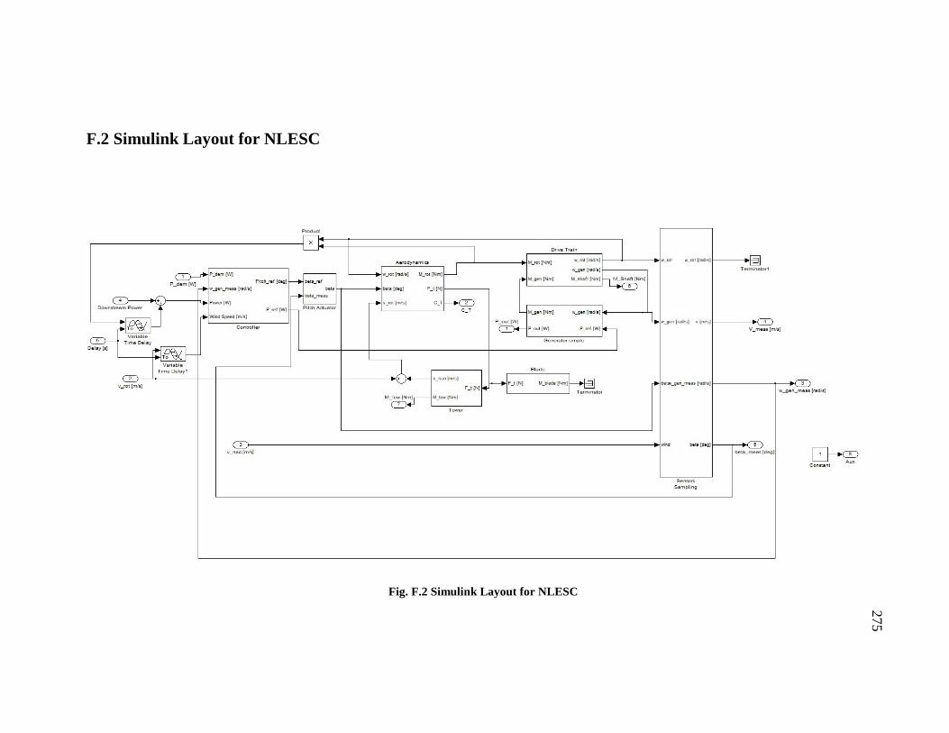
275
F.2 Simulink Layout for NLESC
Fig. F.2 Simulink Layout for NLESC

276
F.3 Simulink Layout Template Generated by SimWindFarm
Fig. F.3 Simulink Layout Template Generated by SimWindFarm
CT
V_nac [m/s]
V_rot [m/s]
Wind Field
P_dem [W]
V_rot [m/s]
V_nac [m/s]
P
V_nac_meas [m/s]
w _gen
pitch
aux
CT
P_dem [W]
V_rot [m/s]
V_nac [m/s]
P [W]
V_meas [m/s]
w_gen [m/s]
Pitch [deg]
Aux
CT
Turbines
Total power
Time
To Workspace9
PowerDemand
To Workspace8
GenSpeed
To Workspace7
FarmPowerDemand
To Workspace6
WindNac
To Workspace5
WindEff
To Workspace4
TotalPower
To Workspace3
Pitch
To Workspace2
PowerAvailable
To Workspace10
Power
To Workspace1
Scope3
Scope2Scope1
PowerAvailable
Power Demand
Power
Post processing
Pitch
P_farm_dem [W]
P_avail[W]
f_grid [Hz]
Network OperatorP_grid[W]
Network Load
Generated Pow er [W]
Consumed Pow er [W]
Grid Frequency [Hz]
P_farm [W]
P_grid [W]
f_grid [Hz]
Grid
Generator Speed
P_meas [W]
V_meas [m/s]
w_rot [rad/s]
Pitch [deg]
Aux
P_farm_dem [W]
P_dem[W]
P_avail [W]
Farm Control
DisplayClock

277
Appendix G. Default Wind Farm Controller in SimWindFarm
In default wind farm control of SimWindFarm, the power demands for turbines are
proportionally to the available power of every turbine [191]
3, ,max
12a i i pP AV Cρ= (G.1)
,a a iP P=∑ (G.2)
where Pa,i is the available power for turbine i, vi is the wind speed at the nacelle of turbine
i, Cp,max is the maximum power coefficient of the turbine. Note that in reference [191],
Cp,max is denoted as maximum thrust coefficient, which the author considers as a typo.
Then, the power demand to the i-th turbine is determined as
,,
a id i d
a
PP P
P= (G.3)
where Pd is the farm-level power demand.

278
Reference
[1] Global_Wind_Energy_Council, "Global wind statistics 2012," Website: http://www.gwec.net/wp-content/uploads/2013/02/GWEC-PRstats-2012_english.pdf, 2013.
[2] "Strengthening America's Energy Security with Offshore Wind," U.S. Department of EnergyFebruary 2011.
[3] Wikipedia. Wind turbine design. Available: http://en.wikipedia.org/wiki/Wind_turbine_design
[4] T. Burton, D. Sharpe, N. Jenkins, and E. Bossanyi, Wind Energy Handbook: John Wiley, 2001.
[5] J. F. Manwell, J. G. McGowan, and A. L. Rogers, Wind Energy Explained, 2nd ed.: Wiley Online Library, 2009.
[6] Wikipedia. Darrieus Wind Turbine. Available: http://en.wikipedia.org/wiki/Darrieus_wind_turbine
[7] J. Creaby, "Maximizing Wind Power Capture Using Multi-variable Extremum Seeking Control," Master of Science, Mechanical Engineering, Universtiy of Wisconsin-Milwaukee, Milwaukee, WI,USA, 2008.
[8] J. Creaby, Y. Li, and J. E. Seem, "Maximizing wind turbine energy capture using multivariable extremum seeking control," Wind Engineering, vol. 33, pp. 361-387, 2009.
[9] K. E. Johnson, L. J. Fingersh, M. J. Balas, and L. Y. Pao, "Methods for increasing region 2 power capture on a variable-speed wind turbine," Journal of Solar Energy Engineering, vol. 126, p. 1092, 2004.
[10] E. Bossanyi, "Individual blade pitch control for load reduction," Wind energy, vol. 6, pp. 119-128, 2003.
[11] K. Selvam, S. Kanev, J. van Wingerden, T. Van Engelen, and M. Verhaegen, "Feedback–feedforward individual pitch control for wind turbine load reduction," International Journal of Robust and Nonlinear Control, vol. 19, pp. 72-91, 2009.
[12] T. J. Larsen, H. A. Madsen, and K. Thomsen, "Active load reduction using individual pitch, based on local blade flow measurements," Wind energy, vol. 8, pp. 67-80, 2005.
[13] P. Sørensen, A. D. Hansen, F. Iov, F. Blaabjerg, and M. H. Donovan, "Wind farm models and control strategies," Risø National Laboratory Risø-R-1464(EN), August 2005.
[14] R. Fernandez, P. Battaiotto, and R. Mantz, "Wind farm non-linear control for damping electromechanical oscillations of power systems," Renewable Energy, vol. 33, pp. 2258-2265, 2008.
[15] J. Rodriguez-Amenedo, S. Arnaltes, and M. Rodriguez, "Operation and coordinated control of fixed and variable speed wind farms," Renewable Energy, vol. 33, pp. 406-414, 2008.

279
[16] K. E. Johnson and N. Thomas, "Wind farm control: Addressing the aerodynamic interaction among wind turbines," in American Control Conference, Hyatt Regency Riverfront, St. Louis, MO, US, 2009, pp. 2104-2109.
[17] N. Jensen, "A note on wind turbine interaction," Risø National Laboratory, DK-4000 Roskilde, Denmark, Risø-M-2411, 1983.
[18] G. C. Larsen, H. A. Madsen, K. Thomsen, and T. J. Larsen, "Wake meandering: a pragmatic approach," Wind energy, vol. 11, pp. 377-395, 2008.
[19] S. J. Qin and T. A. Badgwell, "A survey of industrial model predictive control technology," Control engineering practice, vol. 11, pp. 733-764, 2003.
[20] M. Kuure-Kinsey and B. W. Bequette, "Multiple Model Predictive Control of Nonlinear Systems," in Nonlinear model predictive control: Towards new challenging applications. vol. 384, ed: Springer-Verlag New York Incorporated, 2009.
[21] G. P. Corten and P. Schaak, "More Power and Less Loads in Wind Farms:'Heat and Flux'," in European Wind Energy Conference, London,UK, 2004.
[22] J. E. Seem and Y. Li, "Systems and Methods for Optimizing Power Generation in a Wind Farm Turbine Array," USA Patent, (pending), 2012.
[23] V. Spudic, "Hierarchical wind farm control for power/load optimization," in The Science of making Torque from Wind, 2010.
[24] M. Soleimanzadeh and R. Wisniewski, "Controller design for a wind farm, considering both power and load aspects," Mechatronics, vol. 21, pp. 720-727, 2011.
[25] J. R. Marden, S. D. Ruben, and L. Y. Pao, "A Model-Free Approach to Wind Farm Control Using Game Theoretic Methods," presented at the Proceedings of the 2012 AIAA/ASME Wind Energy Symposium, Nashville, Tennessee, 2012.
[26] W. E. Heronemus, "Pollution-free energy from offshore winds," in 8th Annual Conference and Exposition Marine Technology Society, Washington D.C., 1972.
[27] D. Biester. (2009). Hywind: Siemens and StatoilHydro Install First Floating Wind Turbine. Available: http://www.siemens.com/press/en/pressrelease/?press=/en/pressrelease/2009/renewable_energy/ERE200906064.htm
[28] J. M. Jonkman, "Dynamics modeling and loads analysis of an offshore floating wind turbine," PhD, University of Colorado, Boulder, 2007.
[29] R. G. Sullivan, L. B. Kirchler, J. Cothren, and S. L. Winters, "Preliminary Assessment of Offshore Wind Turbine Visibility and Visual Impact Threshold Distances."
[30] M. Schwartz, D. Heimiller, S. Haymes, and W. Musial, "Assessment of Offshore Wind Energy Resources for the United States," National Renewable Energy Laboratory (NREL), Golden, CO. NREL/TP-500-45889, June 2010.
[31] S. Butterfield, W. Musial, J. Jonkman, P. Sclavounos, and L. Wayman, "Engineering challenges for floating offshore wind turbines," in The 2005 Copenhagen Offshore Wind Conference, Copenhagen, Denmark, 2005.
[32] T. J. Larsen and T. D. Hanson, "A method to avoid negative damped low frequent tower vibrations for a floating, pitch controlled wind turbine," Journal of Physics: Conference Series, vol. 75, p. 012073, 2007.

280
[33] M. A. Lackner and M. A. Rotea, "Structural control of floating wind turbines," Mechatronics, vol. 21, pp. 704-819, Jun 2011.
[34] S. Colwell and B. Basu, "Tuned liquid column dampers in offshore wind turbines for structural control," Engineering Structures, vol. 31, pp. 358-368, 2009.
[35] Y. Li, "Active Vane Control for Stabilization of Offshore Floating Wind Turbines," Invention Disclosure, 2013.
[36] S. J. Johnson, C. Van Dam, and D. E. Berg, "Active load control techniques for wind turbines," SAND2008-4809, Sandia National Laboratories, Albuquerque, NM, 2008.
[37] E. Bossanyi, "The design of closed loop controllers for wind turbines," Wind energy, vol. 3, pp. 149-163, 2000.
[38] T. Olsen, E. Lang, A. Hansen, M. Cheney, G. Quandt, J. VandenBosche, and T. Meyer, "Low Wind Speed Turbine Project Conceptual Design Study: Advanced Independent Pitch Control," National Renewable Energy Laboratory NREL/SR-500-3675, 2004.
[39] M. Hand, A. Wright, L. Fingersh, and M. Harris, "Advanced wind turbine controllers attenuate loads when upwind velocity measurements are inputs," 2006.
[40] S. Kanev and T. van Engelen, "Exploring the limits in individual pitch control," in 2009 European Wind Energy Conference (EWEC 2009), Marseille, France, 2009, pp. 16-19.
[41] M. Jelavic, V. Petrovic, and N. Peric, "Individual pitch control of wind turbine based on loads estimation," in Industrial Electronics, 2008. IECON 2008. 34th Annual Conference of IEEE, 2008, pp. 228-234.
[42] T. Van Engelen, "Design model and load reduction assessment for multi-rotational mode individual pitch control (higher harmonics control)," in European Wind Energy Conference, 2006, pp. 27.2-2.3.
[43] E. Bossanyi and A. Wright, "Field testing of individual pitch control on the NREL CART-2 wind turbine," in EWEC2009-European Wind Energy Conference & Exhibition, 2009.
[44] E. Bossanyi, A. Wright, and P. Fleming, "Progress with field testing of individual pitch control," in Conference on the science of making torque from wind, The European Academy of Wind Energy, 2010.
[45] E. Bossanyi, A. Wright, and P. Fleming, "Further progress with field testing of individual pitch control," in Proc. of the European Wind Energy Conference, EWEC, 2010.
[46] A. Wright, L. Fingersh, and K. Stol, "Designing and testing controls to mitigate tower dynamic loads in the controls advanced research turbine," National Renewable Energy Laboratory NREL/CP-500-40932, 2007.
[47] M. Geyler and P. Caselitz, "Individual blade pitch control design for load reduction on large wind turbines," in Proceeding of the European Wind Energy Conference, Milan, Italy, 2007, pp. 82-86.
[48] M. A. Lackner and G. van Kuik, "A comparison of smart rotor control approaches using trailing edge flaps and individual pitch control," Wind energy, vol. 13, pp. 117-134, 2010.
281
[49] M. J. Balas, Y. J. Lee, and L. Kendall, "Disturbance tracking control theory with application to horizontal axis wind turbines," in Proceedings of the 17th ASME Wind Energy Symposium, Reno, NV, 1998, pp. 95-99.
[50] K. A. Stol, "Dynamics modeling and periodic control of horizontal-axis wind turbines," PhD, Department of Aerospace Engineering Sciences, University of Colorado, 2001.
[51] M. M. Hand, "Mitigation of wind turbine/vortex interaction using disturbance accommodating control," National Renewable Energy Laboratory NREL/TP-500-35172, 2003.
[52] A. D. Wright, "Modern control design for flexible wind turbines," PhD, University of Colorado, 2004.
[53] A. Wright and L. Fingersh, "Advanced Control Design for Wind Turbines," Technical Report NREL/TP-500-42437, National Renewable Energy Laboratory2008.
[54] A. Wright and K. A. Stol, "Designing and testing controls to mitigate dynamic loads in the controls advanced research turbine," in Conference Paper 2008 ASME Wind Energy Symposium, 2008.
[55] W. Zhao and K. Stol, "Individual Blade Pitch for Active Yaw Control of a Horizontal-Axis Wind Turbine," in 45th AIAA Aerospace Sciences Meeting and Exhibit, 2007, pp. 8-11.
[56] H. Namik and K. Stol, "Individual blade pitch control of a floating offshore wind turbine on a tension leg platform," in 48th AIAA Aerospace Science Meeting and Exhibit, 2010.
[57] A. Crespo, J. Hernandez, and S. Frandsen, "Survey of modelling methods for wind turbine wakes and wind farms," Wind energy, vol. 2, pp. 1-24, 1999.
[58] R. Templin, "An estimation of the interaction of windmills in widespread arrays," National Aeronautical Establishment, Laboratory Report LTR-LA, vol. 171, 1974.
[59] B. Newman, "The spacing of wind turbines in large arrays," Energy Conversion, vol. 16, pp. 169-171, 1977.
[60] C. Crafoord, "Interaction in limited arrays of windmills," NASA STI/Recon Technical Report N, vol. 83, p. 13608, 1979.
[61] D. Moore, "Depletion of available wind power by a large network of wind generators," presented at the International Conference on Future Energy Concepts, London, England, 1979.
[62] E. Bossanyi, G. Whittle, P. Dunn, N. Lipman, P. Musgrove, and C. Maclean, "The efficiency of wind turbine clusters," 1980, pp. 401-416.
[63] S. Frandsen, "On the wind speed reduction in the center of large clusters of wind turbines," Journal of Wind Engineering and Industrial Aerodynamics, vol. 39, pp. 251-265, 1992.
[64] S. Emeis and S. Frandsen, "Reduction of horizontal wind speed in a boundary layer with obstacles," Boundary-Layer Meteorology, vol. 64, pp. 297-305, 1993.
[65] P. Lissaman, "Energy effectiveness of arbitrary arrays of wind turbines," in 17th American Institute of Aeronautics and Astronautics, Aerospace Sciences Meeting, New Orleans, LA, 1979.
[66] P. Vermeulen and P. Builtjes, "Mathematical modelling of wake interaction in wind turbine arrays part II," MT-TNO Report 81, vol. 2834, 1981.

282
[67] I. Katic, J. Højstrup, and N. Jensen, "A simple model for cluster efficiency," European Wind Energy Association, pp. 407-409, 1986.
[68] S. Frandsen, R. Barthelmie, S. Pryor, O. Rathmann, S. Larsen, J. Højstrup, and M. Thøgersen, "Analytical modelling of wind speed deficit in large offshore wind farms," Wind energy, vol. 9, pp. 39-53, 2006.
[69] G. C. Larsen, J. Højstrup, and H. A. Madsen, "Wind fields in wakes," EWEC 1996 Proceedings, Goteborg (Sweden), 1996.
[70] H. Schlighting and K. Gersten, Boundary-layer theory: Springer; 8th edition (March 22, 2000), 1979.
[71] P. Sforza, W. Stasi, M. Smorto, and P. Sheerin, "Wind turbine generator wakes," in 17th American Institute of Aeronautics and Astronautics, Aerospace Sciences Meeting, New Orleans, LA, 1979.
[72] P. Taylor, "On wake decay and row spacing for WECS farms," in 3rd International Symposium on Wind Energy Systems, Lyngby, Denmark, 1980, pp. 451-468.
[73] M. K. Liu, M. Yocke, and T. Myers, "Mathematical model for the analysis of wind-turbine wakes," Journal of Energy, vol. 7, pp. 73-78, 1983.
[74] J. F. Ainslie, "Calculating the flowfield in the wake of wind turbines," Journal of Wind Engineering and Industrial Aerodynamics, vol. 27, pp. 213-224, 1988.
[75] A. Duckworth and R. Barthelmie, "Investigation and Validation of Wind Turbine Wake Models," Wind Engineering, vol. 32, pp. 459-475, 2008.
[76] D. J. Renkema, "Validation of wind turbine wake models," Master, TU Delft, 2007.
[77] L. Rademakers, F. van Hulle, and W. Stam, European wind turbine standards: Netherlands Energy Research Foundation ECN, 1996.
[78] J. Van Leuven, "The Energetic Effectiveness of A Cluster of Wind Turbines," PhD, Catholic University of Louvain, 1992.
[79] U. Högström, D. Asimakopoulos, H. Kambezidis, C. Helmis, and A. Smedman, "A field study of the wake behind a 2 MW wind turbine," Atmospheric Environment (1967), vol. 22, pp. 803-820, 1988.
[80] G. C. Larsen, H. Madsen Aagaard, F. Bingöl, J. Mann, S. Ott, J. N. Sørensen, V. Okulov, N. Troldborg, N. M. Nielsen, K. Thomsen, T. J. Larsen, and R. Mikkelsen, "Dynamic wake meandering modeling," Risø National Laboratory Risø-R-1607(EN) 2007.
[81] D. Medici and P. Alfredsson, "Measurements on a wind turbine wake: 3D effects and bluff body vortex shedding," Wind energy, vol. 9, pp. 219-236, 2006.
[82] K. Thomsen, Madsen, H., Larsen, G. and Larsen, T., "A Simplified Approach for Simulation of Wake Meandering," Risø National Laboratory RISO Report AED-RB-18, 2006.
[83] J. J. Trujillo and M. Kühn, "Adaptation of a lagrangian dispersion model for wind turbine wake meandering simulation," in European Wind Energy Conference (EWEC), Marseille, France, 2009.
[84] A. Jimenez, A. Crespo, E. Migoya, and J. Garcia, "Advances in large-eddy simulation of a wind turbine wake," Journal of Physics: Conference Series, vol. 75, p. 012041, 2007.

283
[85] P. S. Veers, "Three-dimensional wind simulation," Sandia National Labs., Albuquerque, NM, USA, SAND88-0152, 1988.
[86] M. Nielsen, G. C. Larsen, and K. Hansen, "Simulation of inhomogeneous, non-stationary and non-Gaussian turbulent winds," Journal of Physics: Conference Series, vol. 75, p. 012060, 2007.
[87] G. Espana, S. Aubrun, and P. Devinant, "Is the Meandering of a Wind Turbine Wake Due to Atmospheric Length Scales?," Progress in Turbulence III, pp. 91-94, 2009.
[88] L. Kristensen and N. Jensen, "Lateral coherence in isotropic turbulence and in the natural wind," Boundary-Layer Meteorology, vol. 17, pp. 353-373, 1979.
[89] A. Davenport, "The prediction of the response of structures to gusty wind," Safety of Structures under Dynamic Loading, vol. 1, pp. 257-284, 1977.
[90] H. A. Madsen, G. C. Larsen, T. J. Larsen, N. Troldborg, and R. Mikkelsen, "Calibration and validation of the Dynamic Wake Meandering model for implementation in an aeroelastic code," Journal of Solar Energy Engineering, vol. 132, p. 041014, 2010.
[91] I. E. Committee, "IEC 61400-1: Wind turbines part 1: Design Requirements," ed: IEC, 2005.
[92] J. A. Rossiter, Model-based predictive control: a practical approach: CRC, 2003. [93] E. F. Camacho and C. Bordons, Model predictive control: Springer-Verlag
London, 2003. [94] W. H. Kwon and S. H. Han, Receding horizon control: model predictive control
for state models: Springer, 2005. [95] J. B. Rawlings and D. Q. Mayne, Model Predictive Control: Theory and Design:
NOb Hill Pub, 2009. [96] F. Borrelli, Bemporad, A., and Morari, M., Predictive control for linear and
hybrid systems: Cambridge University Press, 2012. [97] D. Q. Mayne, J. B. Rawlings, C. V. Rao, and P. O. M. Scokaert, "Constrained
model predictive control: Stability and optimality," Automatica, vol. 36, pp. 789-814, 2000.
[98] A. Bemporad and M. Morari, "Robust model predictive control: A survey," Robustness in identification and control, pp. 207-226, 1999.
[99] W. Kwon and A. Pearson, "A modified quadratic cost problem and feedback stabilization of a linear system," Automatic Control, IEEE Transactions on, vol. 22, pp. 838-842, 1977.
[100] W. Kwon and A. Pearson, "On feedback stabilization of time-varying discrete linear systems," Automatic Control, IEEE Transactions on, vol. 23, pp. 479-481, 1978.
[101] S. Keerthi and E. G. Gilbert, "Optimal infinite-horizon feedback laws for a general class of constrained discrete-time systems: Stability and moving-horizon approximations," Journal of optimization theory and applications, vol. 57, pp. 265-293, 1988.
[102] J. B. Rawlings and K. R. Muske, "The stability of constrained receding horizon control," Automatic Control, IEEE Transactions on, vol. 38, pp. 1512-1516, 1993.

284
[103] A. Zheng and M. Morari, "Stability of model predictive control with mixed constraints," Automatic Control, IEEE Transactions on, vol. 40, pp. 1818-1823, 1995.
[104] P. Scokaert and J. B. Rawlings, "Infinite horizon linear quadratic control with constraints," in Proceedings of the 13th IFAC World Congress, San Francisco, 1996.
[105] E. Polak and T. Yang, "Moving horizon control of linear systems with input saturation and plant uncertainty part 1. robustness," International Journal of Control, vol. 58, pp. 613-638, 1993.
[106] Z. Q. Zheng, "Robust Control of Systems Subject to Constraints," PhD, California Institute of Technology, Pasadena,CA, 1995.
[107] L. C. Henriksen, "Model predictive control of a wind turbine," Technical University of Denmark, DTU, IMM-Thesis, 2007.
[108] R. A. Santos, "Damage mitigating control for wind turbines," PhD, Department of Aerospace Engineering Sciences, University of Colorado at Boulder, Boulder, 2007.
[109] A. A. Kumar and K. A. Stol, "Scheduled model predictive control of a wind turbine," ed: American Institute of Aeronautics and Astronautics, 1801 Alexander Bell Dr., Suite 500 Reston VA 20191-4344 USA, 2009.
[110] J. Laks, L. Y. Pao, E. Simley, A. Wright, N. Kelley, and B. Jonkman, "Model predictive control using preview measurements from lidar," in 49th AIAA Aerospace Sciences Meeting, Orlando, Florida, 2011.
[111] M. Soltani, R. Wisniewski, P. Brath, and S. Boyd, "Load reduction of wind turbines using receding horizon control," in Control Applications (CCA), 2011 IEEE International Conference, Denver, CO 2011, pp. 852-857.
[112] Y. Wang and S. Boyd, "Fast model predictive control using online optimization," Control Systems Technology, IEEE Transactions on, vol. 18, pp. 267-278, 2010.
[113] D. Castaignet, N. K. Poulsen, T. Buhl, and J. J. Wedel-Heinen, "Model Predictive Control of Trailing Edge Flaps on a wind turbine blade," in American Control Conference (ACC), 2011 San Francisco, CA 2011, pp. 4398-4403.
[114] A. A. Kumar and K. A. Stol, "Scheduled model predictive control of a wind turbine," in 28th American Society of Mechanical Engineers (ASME) Wind Energy Symposiu, Orlando, Florid, 2009.
[115] S. Joe Qin, V. M. Martínez, and B. A. Foss, "An interpolating model predictive control strategy with application to a waste treatment plant," Computers & Chemical Engineering, vol. 21, pp. S881-S886, 1997.
[116] D. Dougherty and D. Cooper, "A practical multiple model adaptive strategy for single-loop MPC," Control engineering practice, vol. 11, pp. 141-159, 2003.
[117] D. Dougherty and D. Cooper, "A practical multiple model adaptive strategy for multivariable model predictive control," Control engineering practice, vol. 11, pp. 649-664, 2003.
[118] J. Wang, "Softly Switched Model Predictive Control: Generic Development and Application to Water Supply and Distribution Systems," PhD, Mechanical Department, Univerisity of Birmingham, 2006.

285
[119] S. Di Cairano, E. Tseng, D. Bernardini, and A. Bemporad, "Steering vehicle control by switched model predictive control," in Advances in Automotive Control, 2010, pp. 1-6.
[120] P. Mhaskar, N. H. El-Farra, and P. D. Christofides, "Predictive Control of Switched Nonlinear Processes with Scheduled Mode Transitions," in Dynamics and Control of Process Systems 2004 (DYCOPS-7): A Proceedings Volume from the 7th IFAC Symposium, Cambridge, Massachusetts, USA, 5-7 July 2004, p. 257.
[121] L. Özkan and M. V. Kothare, "Stability analysis of a multi-model predictive control algorithm with application to control of chemical reactors," Journal of Process Control, vol. 16, pp. 81-90, 2006.
[122] M. Kuure-Kinsey, "Novel Approaches to Nonlinear Model Preidictive Control with Application to High Temperature Fuel Cells," PhD, Chemical Engineering, Rensselaer Polytechnic Institute, 2008.
[123] R. R. Rao, B. Aufderheide, and B. W. Bequette, "Experimental studies on multiple-model predictive control for automated regulation of hemodynamic variables," Biomedical Engineering, IEEE Transactions on, vol. 50, pp. 277-288, 2003.
[124] H. Ferreau, "qpOASES–an open-source implementation of the online active set strategy for fast model predictive control," 2007, pp. 29-30.
[125] A. Bemporad, M. Morari, V. Dua, and E. N. Pistikopoulos, "The explicit linear quadratic regulator for constrained systems," Automatica, vol. 38, pp. 3-20, 2002.
[126] M. de la Pena, A. Bemporad, and C. Filippi, "Robust explicit MPC based on approximate multi-parametric convex programming," 2004, pp. 2491-2496 Vol. 3.
[127] H. J. Ferreau, E. Arnold, H. Diedam, H. J. Ferreau, B. Houska, C. Kirches, A. Perrin, A. Potschka, T. Wiese, and L. Wirsching, "qpOASES User's Manual," Optimization in Engineering Center (OPTEC) and Department of Electrical Engineering, K. U. Leuve,2011.
[128] G. Associates, "Unique Integration of Mature Technologies," in 16th Offshore Symposium, Houston, TX, 2010.
[129] G. R. Fulton, D. J. Malcolm, and E. Moroz, "Design of a Semi-Submersible Platform for a 5MW Wind Turbine," in Proceeding 44th AIAA/ASME Wind Energy Symposium, Reno, NV, 2006.
[130] K. H. Lee, "Responses of floating wind turbines to wind and wave excitation," MSc. Thesis, Massachusetts Institute of Technology, 2005.
[131] Sway to Erect 10 MW Offshore Wind Turbine, May 30, 2010. Available: http://www.renewableenergyfocus.com/view/7279/sway-to-erect-10-mw-offshore-wind-turbine/
[132] B. Bulder, M. T. van Hees, A. Henderson, R. Huijsmans, J. Pierik, E. Snijders, G. Wijnants, and M. Wolf, "Study to feasibility of and boundary conditions for floating offshore wind turbines," ECN,MARIN, Largerweij the Windmaster, TNO and TUD 2002-CMC-R43, 2002.
[133] W. Musial, and Ram, B., "Large-Scale Offshore Wind Power in the United States: Assessment of Oppportunities and Barriers," National Renewable Energy Laboratory, Boulder, Colorado NREL/TP-500-40745, September 2010.
[134] PrinciplePower. Principle Power's WindFloat. Available: http://www.youtube.com/watch?v=IO7GXLR4YUo

286
[135] B. Linde, "Motion of floating wind turbines," M.Sc., Norwegian University of Science and Technology, 2010.
[136] J. E. Withee, "Fully coupled dynamic analysis of a floating wind turbine system," PhD, Massachusetts Institute of Technology, 2004.
[137] "ADAMS User's Guide," Mechanical Dynamics, Inc., Ann Arbor, MI2002. [138] P. J. Moriarty and A. C. Hansen, "Aerodyn theory manual," National Renewable
Energy Laboratory NREL/TP-500-3688, 2005. [139] E. Wayman, "Coupled Dynamics and Economic Analysis of Floating Wind
Turbine Systems," Master of Science, Mechanical Engineering, Massachusetts Institute of Technology, 2006.
[140] J. M. Jonkman and M. L. Buhl Jr, "FAST user’s guide," National Renewable Energy Lab, Golden, Colorado, USA NREL/EL-500-38230, 2005.
[141] D. Matha, "Model Development and Loads Analysis of an Offshore Wind Turbine on a Tension Leg Platform with a Comparison to Other Floating Turbine Concepts," Master, University of Colorado, Boulder, 2009.
[142] C. Cermelli, D. Roddier, and A. Aubault, "WINDFLOAT: a floating foundation for offshore wind turbines Part II: Hydrodynamics analysis," in Proceedings of the ASME 28th International Conference on Ocean, Offshore and Arctic Engineering, Honolulu, Hawaii, USA, 2009.
[143] D. Roddier, C. Cermelli, A. Aubault, and A. Weinstein, "WindFloat: A floating foundation for offshore wind turbines," Journal of Renewable and Sustainable Energy, vol. 2, p. 033104, 2010.
[144] C. H. Lee, WAMIT theory manual: Massachusetts Institute of Technology, Dept. of Ocean Engineering, 1995.
[145] F. G. Nielsen, T. D. Hanson, and B. Skaare, "Integrated dynamic analysis of floating offshore wind turbines," in Proceedings of the 25th International Conference on Offshore Mechanics and Artic Engineering, Hamburg, German, 2006, pp. 671-679.
[146] T. J. Larsen and A. M. Hansen, "How 2 HAWC2, the user's manual," Risø National Laboratory 8755035833, 2007.
[147] S. Reinholdtsen and E. Falkenberg, "SIMO General Description," Marintek Report MTK, vol. 519614, 1998.
[148] I. Fylling, C. Larsen, N. Sødahl, E. Passano, A. Bech, A. Engseth, H. Lie, and H. Ormberg, "RIFLEX User’s Manual 3.6," 2008.
[149] J. M. Jonkman, "Influence of control on the pitch damping of a floating wind turbine," in the 2008 ASME Wind Energy Symposium, Reno, Nevada, 2008.
[150] B. Skaare, T. D. Hanson, and F. G. Nielsen, "Importance of control strategies on fatigue life of floating wind turbines," in 26th International Conference on Offshore Mechanics and Arctic Engineering, San Diego, California, 2007.
[151] H. Namik and K. Stol, "Individual blade pitch control of floating offshore wind turbines," Wind energy, vol. 13, pp. 74-85, 2010.
[152] H. Namik and K. Stol, "Performance analysis of individual blade pitch control of offshore wind turbines on two floating platforms," Mechatronics, vol. 21, pp. 691-703, 2011.
[153] M. A. Lackner and M. A. Rotea, "Passive structural control of offshore wind turbines," Wind energy, vol. 14, pp. 373-388, 2011.

287
[154] N. Luo, C. Bottasso, H. Karimi, and M. Zapateiro, "Semiactive Control for Floating Offshore Wind Turbines Subject to Aero-hydro Dynamic Loads," presented at the International Conference on Renewable Energies and Power Quality, Las Palmas de Gran Canaria, Spain, 2011.
[155] Z. Yang, Y. Li, and J. E. Seem, "Individual Pitch Control for Wind Turbine Load Reduction Including Wake Modeling," Wind Engineering, vol. 35, pp. 715-738, 2012.
[156] Z. Yang, Y. Li, and J. E. Seem, "Load Reduction of Wind Turbines under Wake Meandering with Model Predictive Control for Individual Pitching," in 50th AIAA Aerospace Sciences Meeting including the New Horizons Forum and Aerospace Exposition, Nashville, Tennessee, 2012.
[157] C. J. Spruce, "Simulation and control of windfarms," PhD, University of Oxford, 1993.
[158] F. Borrelli, Constrained optimal control of linear and hybrid systems vol. 290: Springer Verlag, 2003.
[159] M. Soltani, T. Knudsen, and T. Bak, "Modeling and Simulation of Offshore Wind Farms for Farm Level Control," in European Offshore Wind Conference and Exhibition (EOW) 2009, Stockholm, Sweden, 2009.
[160] M. Soleimanzadeh and R. Wisniewski, "An optimal control scheme to minimize loads in wind farms," in Control Applications (CCA), 2012 IEEE International Conference on, 2012, pp. 986-990.
[161] D. Madjidian and A. Rantzer, "A stationary turbine interaction model for control of wind farms," in IFAC 18th World Congress, Milano, Italy, 2011.
[162] A. J. Brand, "A Quasi-Steady Wind Farm Control Model," in European Wind Energy Conference, Brussels,Belgium, 2011.
[163] A. J. Brand and J. W. Wagenaar, "A quasi-steady wind farm flow model in the context of distributed control of the wind farm," in European Wind Energy Conference, 2010.
[164] T. Knudsen, T. Bak, and M. Soltani, "Distributed control of large-scale offshore wind farms," in Eropean Wind Energy Conference, Marseille, France, 2009.
[165] M. Kristalny and D. Madjidian, "Decentralized feedforward control of wind farms: prospects and open problems," in Decision and Control and European Control Conference (CDC-ECC), 2011 50th IEEE Conference on, 2011, pp. 3464-3469.
[166] D. Madjidian, K. Martensson, and A. Rantzer, "A distributed power coordination scheme for fatigue load reduction in wind farms," in American Control Conference (ACC), 2011, pp. 5219-5224.
[167] D. Madjidian, M. Kristalny, and A. Rantzer, "Dynamic Power Coordination for Load Reduction in Dispatchable Wind Power Plants," in 2013 European Control Conference, Zürich, Switzerland, July 2013.
[168] B. Biegel, D. Madjidian, V. Spudic, A. Rantzer, and J. Stoustrup, "Distributed low-complexity controller for wind power plant in derated operation," in IEEE Multi-Conference on Systems and Control, Hyderabad, India, 2013.
[169] R. Zhao, W. Shen, T. Knudsen, and T. Bak, "Fatigue distribution optimization for offshore wind farms using intelligent agent control," Wind energy, vol. 15, pp. 927-944, 2012.

288
[170] T. Horvat, V. Spudic, and M. Baotic, "Quasi-stationary optimal control for wind farm with closely spaced turbines," in MIPRO, 2012 Proceedings of the 35th International Convention, 2012, pp. 829-834.
[171] E. Bitar and P. Seiler, "Coordinated control of a wind turbine array for power maximization," in American Control Conference (ACC), 2013, 2013, pp. 2898-2904.
[172] J. Park, S. Kwon, and K. H. Law, "Wind farm power maximization based on a cooperative static game approach," in SPIE Smart Structures and Materials+ Nondestructive Evaluation and Health Monitoring, 2013, pp. 86880R-86880R-15.
[173] Y. Guo, W. Wang, C. Y. Tang, J. N. Jiang, and R. G. Ramakumar, "Model predictive and adaptive wind farm power control," in American Control Conference (ACC), 2013, pp. 2890-2897.
[174] E. Bossanyi, T. Burton, D. Sharpe, and N. Jenkins, "Wind Energy Handbook," John W iley, 2000.
[175] P. Vermeulen, "An experimental analysis of wind turbine wakes," in 3rd International Symposium on Wind Energy Systems, 1980, pp. 431-450.
[176] B. J. Jonkman, "TurbSim User's Guide: Version 1.50," National Renewable Energy Laboratory NREL/TP-500-46198, 2009.
[177] M. Harris, M. Hand, and A. Wright, "Lidar for turbine control," National Renewable Energy Laboratory, Golden, CO NREL/TP-500-39154, 2006.
[178] F. Haugen. (2008). Derivation of a Discrete-Time Low pass Filter. Available: http://techteach.no/simview/lowpass_filter/doc/filter_algorithm.pdf
[179] K. A. Stol, "Disturbance tracking and blade load control of wind turbines in variable-speed operation," in 22nd ASME Wind Energy Conference, Reno, NV, 2003, pp. 317-322.
[180] L. J. Fingersh and K. E. Johnson, "Controls advanced research turbine (CART) commissioning and baseline data collection," National Renewable Energy Laboratory NREL/TP-500-32879, 2002.
[181] G. Bir, "Multiblade coordinate transformation and its application to wind turbine analysis," in Proceedings of 2008 ASME Wind Energy Symposium, Reno, Nevada, USA, Jan. 7, 2008.
[182] L. C. Henriksen, N. K. Poulsen, and H. H. Niemann, "Constraint handling within a multi-blade coordinate framework of a wind turbine," in Decision and Control and European Control Conference (CDC-ECC), 2011 50th IEEE Conference on, 2011, pp. 5825-5830.
[183] W. Johnson, Helicopter theory. New Jersey: Princeton University Press, 1980. [184] M. Kuure-Kinsey and B. W. Bequette, "Multiple model predictive control: a state
estimation based approach," in American Control Conference, 2007. ACC'07, 2007, pp. 3739-3744.
[185] J. Jonkman, S. Butterfield, W. Musial, and G. Scott, "Definition of a 5-MW reference wind turbine for offshore system development," National Renewable Energy Laboratory, NREL/TP-500-38060, 2009.
[186] J. M. Jonkman and M. L. Buhl Jr, "FAST user’s guide," Rep. No. NREL/EL-500-38230, NREL, Golden, Colorado, USA, 2005.

289
[187] M. A. Rotea, "Analysis of Multivariable Extremum Seeking Algorithms," in Proceeding of 2000 American Control Conference, Chicago, IL, 2000, pp. 433-437.
[188] I. Munteanu, A. I. Bratcu, and E. Ceangǎ, "Wind turbulence used as searching signal for MPPT in variable-speed wind energy conversion systems," Renewable Energy, vol. 34, pp. 322-327, 2009.
[189] T. Pan, Z. Ji, and Z. Jiang, "Maximum power point tracking of wind energy conversion systems based on sliding mode extremum seeking control," in Energy 2030 Conference, 2008. ENERGY 2008. IEEE, Atlanta, GA, 2008, pp. 1-5.
[190] T. Hawkins, W. N. White, G. Hu, and F. D. Sahneh, "Region II wind power capture maximization using robust control and estimation with alternating gradient search," in American Control Conference (ACC), San Francisco, CA, 2011, pp. 2695-2700.
[191] J. D. Grunnet, M. Soltani, T. Knudsen, M. Kragelund, and T. Bak, "Aeolus toolbox for dynamic wind farm model, simulation and control," in Proceedings of the European Wind Energy Conference, Warsaw, Poland, 2010.
[192] J. Jonkman, S. Butterfield, W. Musial, and G. Scott, "Definition of a 5-MW reference wind turbine for offshore system development," National Renewable Energy Laboratory, NREL/TP-500-38060,, 2009.
[193] D. G. Alciatore and M. B. Histand, Introduction to mechatronics and measurement systems: McGraw-Hill New York, 2007.
[194] J. Schepers and S. Pijl, "Improved modelling of wake aerodynamics and assessment of new farm control strategies," Journal of Physics: Conference Series, The Science of Making Torque from Wind, vol. 75, p. 012039, 2007.
[195] J. Jonkman, "Definition of the Floating System for Phase IV of OC3," National Renewable Energy Lab,NREL/TP-500-47535,, May 2010.
[196] J. M. Jonkman and A. C. Hansen, "Development and validation of an aeroelastic model of a small furling wind turbine," in 43 rd AIAA Aerospace Sciences Meeting and Expedition, Reno, Nevada, 2005.
[197] T. R. Kane and D. A. Levinson, Dynamics: Theory and Applications McGraw-Hill, 1985.
[198] R. E. Sheldahl and P. C. Klimas, "Aerodynamic characteristics of seven symmetrical airfoil sections through 180-degree angle of attack for use in aerodynamic analysis of vertical axis wind turbines," Sandia National Labs., Albuquerque, NM (USA), SAND80-2114,1981.
[199] S. Kim, J. J. Alonso, and A. Jameson, "Multi-Element High-Lift Configuration Design Optimization Using Viscous Continuous Adjoint Method," Journal of Aircraft,, vol. 41, pp. 1082-1097, 2004.
[200] G. Hayman, "NWTC Design Codes (MCrunch by Greg Hayman), http://wind.nrel.gov/designcodes/postprocessors/mcrunch/." 2012.

290
CURRICULUM VITAE
Zhongzhou Yang
Place of birth: Linfen, Shanxi, China
Dissertation Title: Wind Turbine Controls for Farm and Offshore Operation
Education:
Bachelor of Engineering, Taiyuan University of Technology, China, June 2004 Major: Engineering Mechanics
Master of Engineering, Beihang University, China, January 2008 Major: Fluid Mechanics
Ph.D., University of Wisconsin-Milwaukee, December 2013 Major: Mechanical Engineering
Employment:
Zhongzhou Yang was working as a Mechanical Engineer at a wind turbine supplier
GoldWind Science and Technology in Beijing, China from April 2007 to September
2008. From October 2008, Zhongzhou started working at the University of Wisconsin-
Milwaukee as research assistant of Prof. Yaoyu Li. From September 2011, Zhongzhou
Yang moved to the University of Texas at Dallas and worked as visiting research
assistant of Prof. Yaoyu Li. From May 2013, Zhongzhou Yang started working as a
Systems Modeling and Control Engineer at Exa Corporation, Livonia, Michigan.
Publications:
[1] Li, Y., Yang, Z., and Seem, J.E., “Active Horizontal Vane Control for Stabilizing
Platform Pitch Motion of Floating Offshore Turbines”, will be presented at AIAA
SciTech 2014, January 13-17th, 2014, National Harbor, Maryland
291
[2] Yang, Z., Li, Y. and Seem, J.E., “Maximizing Wind Farm Energy Capture Via
Nested-Loop Extremum Seeking Control”, Proceedings of 2013 ASME Dynamic
Systems and Control Conference (DSCC’2013), October 21-23, 2013, Stanford
University, Palo Alto, CA
[3] Yang, Z., and Li, Y., “Active Vertical-Vane Control for Roll Motion of Floating
Offshore Wind Turbines”, 51th AIAA Aerospace Sciences Meeting including the
New Horizons Forum and Aerospace Exposition, AIAA 2013-0452, January 9-12th,
2013, Grapevine (Dallas/Ft. Worth Region), Texas
[4] Yang, Z., Li, Y. and Seem, J.E., “Load Reduction of Wind Turbines under Wake
Meandering with Model Predictive Control for Individual Pitching”, 50th AIAA
Aerospace Sciences Meeting including the New Horizons Forum and Aerospace
Exposition, AIAA 2012-1150, January 9-12th, 2012, Nasshville, Tennessee
[5] Yang, Z., Li, Y. and Seem, J.E., “Individual Pitch Control for Wind Turbine Load
Reduction Including Wake Modeling,” Journal of Wind Engineering, 2012,
35(6):715-738
[6] Yang, Z., Li, Y. and Seem, J.E. “Improved Individual Pitch Control for Wind Farm
Turbine Load Reduction via Wake Modeling,” 49th AIAA Aerospace Sciences
Meeting including the New Horizons Forum and Aerospace Exposition, AIAA
2011-820, January 4-7th, 2011, Orlando, Florida
[7] Yang, Z., Li, Y. and Seem, J.E., “Individual pitch control for wind turbine load
reduction including wake interaction”, American Control Conference (ACC), June
29-July 1st, 2011, pp. 5207-5212, San Francisco, CA

292
[8] Yang, Z., Li, Y. and Seem, J.E. “Individual Pitch Control For Wind Turbine Load
Reduction Including Wake Modeling,” Proceedings of 2010 ASME Dynamic
Systems and Control Conference (DSCC’2010), September 13-15, 2010, Cambridge,
MA
[9] Wu, X., Li, Y., Li, F. and Yang, Z. “Adaptive Estimation Based Leakage Detection
for Wind Turbine Hydraulic Pitching System,” IEEE Transactions on Mechatronics,
2012, V17(5): 907-914
[10] Wu, X., Li, Y., Yang, Z., Lu, B. "Model Based Fault Diagnosis for Wind Turbine
Hydraulic Pitching Systems," 2010 American Control Conference, June 30-July 2,
Baltimore, Maryland.
[11] Lu,B., Li,Y., Wu, X. and Yang, Z. “A review of recent advances in wind turbine
condition monitoring and fault diagnosis”, Power Electronics and Machines in
Wind Applications, June 24-26th, 2009, Lincoln, Nebraska
[12] Chen, Q., Li, Y., Seem, J.E., Yang, Z. and Creaby., J. “Self-Optimizing Robust
Control of Wind Power Generation with Doubly-Fed Induction Generator”,
accepted by ASME Journal of Solar Energy Engineering