wind tunnel testing airfoils at low reynolds numbers - aerospace

49th AIAA Aerospace Sciences Meeting AIAA 2011-875 4-7 January 2011, Orlando, FL

Copyright © 2011 by the authors. Published by the American Institute of Aeronautics and Astronautics, Inc., with permission.

Wind Tunnel Testing Airfoils at Low Reynolds Numbers

Michael S. Selig,∗ Robert W. Deters,† and Gregory A. Williamson‡

University of Illinois at Urbana-Champaign, Urbana, IL 61801, USA

This paper describes the wind tunnel testing methodology that has been appliedto testing over 200 airfoils at low Reynolds numbers (40,000 to 500,000). The ex-periments were performed in the 2.8×4.0 ft (0.853×1.219 m) low-turbulence windtunnel in the Subsonic Aerodynamics Research Laboratory at the University of Illi-nois at Urbana-Champaign (UIUC). The test apparatus, methodology, and datareduction techniques are described in detail, and the measurements are validatedagainst benchmark data. New results on the AG455ct airfoil with a large 30%-chordflap, deflected over a wide range, are presented. The results show a dramatic in-crease in drag with higher flap deflections, and the flap efficiency reduces with largedeflections up to 40 deg. Also, tests on a flat-plate airfoil with leading edge serrationgeometries were conducted to explore the effects on stall characteristics. The resultssupport the conclusions of other researchers that leading edge serrations (protuber-ances like those found on the fins/flippers of some aquatic animals) lead to higherlift and softer stall. The results suggest that these characteristics are accompaniedby lower drag in the stall and post-stall range.

I. Introduction

Airfoil performance at low Reynolds numbers impacts the performance of a wide range of systems.The expanding role of unmanned aerial vehicles (UAVs) into unmanned aircraft systems (UAS) in militaryuse1,2 has led to growing interest in subsonic low Reynolds number aerodynamics.3–5 Low Reynolds numberaerodynamics of airfoils also apply to a host of other applications such as wind turbines,6–8 motorsports,high altitude aircraft and propellers, natural flyers,9 and subscale testing of many full scale systems.

Accurate measurements of low Reynolds number airfoil performance is key to understanding and improv-ing the efficiency of low Reynolds number systems. Most aerodynamic performance measurement techniquesfor airfoils rely on using balance systems or pressure systems, or a combination of both.10–12 The approachdescribed in this paper uses a force balance approach to obtain lift and moment data and the wake rakemethod to obtain drag. Sections II and III of this paper describe this experimental approach and validation.Section IV presents first, data on an airfoil with large flap deflections, and second, data on a flat-plate airfoilas compared with one having a range of leading-edge serration geometries. The paper ends with conclusionsthat can be drawn from this research.

II. Wind Tunnel Facility and Measurement Techniques

This section presents detailed descriptions of the UIUC low-turbulence subsonic wind tunnel facility, testsection flow quality, lift, drag and moment measurement techniques, data acquisition equipment, and datareduction procedures that have been documented in Refs. 6,13–16.

∗Associate Professor, Department of Aerospace Engineering, 104 S. Wright St., Senior Member AIAA.http://www.ae.illinois.edu/m-selig

†Graduate Student, Department of Aerospace Engineering, 104 S. Wright St., Student Member AIAA.‡Graduate Student, Department of Aerospace Engineering, 104 S. Wright St., Student Member AIAA.

1 of 32

American Institute of Aeronautics and Astronautics

Figure 1. UIUC low-speed subsonic wind tunnel.

Figure 2. Photograph of wind-tunnel test section.

A. Experimental Facility and Flow Quality Measurements

The low Reynolds number airfoil performance measurements described here were conducted in the UIUClow-turbulence subsonic wind tunnel shown in Fig. 1. The wind tunnel is an open-return type with a 7.5:1contraction ratio. The rectangular test section is nominally 2.8 × 4.0 ft (0.853 × 1.219 m) in cross sectionand 8-ft (2.438-m) long. Over the length of the test section, the width increases by approximately 0.5 in.(1.27 cm) to account for boundary-layer growth along the tunnel sidewalls. Test-section speeds are variableup to 160 mph (71.53 m/s) via a 125-hp (93.25-kW) AC motor connected to a five-bladed fan. For a Reynoldsnumber of 500,000 based on an airfoil chord of 1 ft (0.305 m), the resulting nominal test-section speed is80 ft/sec (24.38 m/s). Photographs of the test section and fan are presented in Figs. 2 and 3

Since low Reynolds number airfoil performance is highly dependent on the behavior of the laminarboundary layer, low turbulence levels within the wind-tunnel test section are necessary to ensure that laminarflow does not prematurely transition to turbulent flow. In order to ensure good flow quality in the test section,the wind-tunnel settling chamber contains a 4-in. (10.16-cm) thick honeycomb in addition to four anti-turbulence screens, which can be partially removed for cleaning. The turbulence intensity was measured andpreviously reported to be less than 0.1%,17 which is sufficient for low Reynolds number airfoil measurements.Subsequent detailed measurements are show later in this section.

The experimental setup is depicted in Fig. 4. For the current tests, the 12-in. (0.305-m) chord, 33 5/8-in.(0.855-m) long airfoil models were mounted horizontally between two 3/8-in. (0.953-cm) thick, 6-ft (1.829-m)

long PlexiglasfRsplitter plates to isolate the ends of the model from the tunnel side-wall boundary layers and

the support hardware. For clarity, the Plexiglas splitter plates and the traverse enclosure box are not shownin Fig. 4. Gaps between the model and Plexiglas were nominally 0.05 in. (1.27 mm). The left-hand side of

2 of 32


figures/wind_tunnel.eps

figures/test_section02.eps

Figure 3. Photograph of wind-tunnel exit fan.

Figure 4. Experimental setup (PlexiglasfRsplitter plates and traverse enclosure box not shown for clarity).

the model was free to pivot (far side of Fig. 4). At this location, the angle of attack was measured using aprecision potentiometer. The right-hand side of the airfoil model was connected to the lift carriage throughtwo steel wing rods that passed through the wing-rod fixture and were anchored to the model through twoset screws. At this side, the airfoil model was free to move vertically on a precision ground shaft, but notfree to rotate. The lift carriage was linked to a custom load beam, as described later. Linear and sphericalball bearings within the lift carriage helped to minimize any frictional effects.

The two-axis traverse can be seen in Fig. 4, positioned above the wind-tunnel test section. Not shownis the pressure-sealed box that encloses the traverse system. The traverse was manufactured by LinTechand consists of horizontal and vertical screw-type linear positioning rails that operate in combination withtwo computer-controlled stepper motors. The rails are equipped with linear optical encoders that supply afeedback signal to the motor controller allowing the traverse to operate with virtually no error. Attached tothe traverse is a 3-ft (0.914-m) long boom that extends down into the wind tunnel test section to supportthe eight side-by-side wake pitot probes [spaced 1.5 in. (3.81-cm) apart in the spanwise direction].

3 of 32


figures/diffuser01.eps

figures/test_section_traverse_open.eps

100,000 200,000 300,000 400,000 500,0000.05

0.1

0.15

0.2

0.25

Reynolds Number

Mea

n T

urbu

lenc

e In

tens

ity (

%)

Average Turbulence Intensity (Empty Test Section)

DC CoupledHPF = 0.1HzHPF = 3HzHPF = 10Hz

100,000 200,000 300,000 400,000 500,0000.05

0.1

0.15

0.2

0.25

Reynolds Number

Mea

n T

urbu

lenc

e In

tens

ity (

%)

Average Turbulence Intensity (Test Apparatus Installed)

DC CoupledHPF = 0.1HzHPF = 3HzHPF = 10Hz

Figure 5. Turbulence intensity at tunnel centerline, empty test section and with rig in place.

1. Turbulence Intensity

The turbulence intensity was previously documented;17 however, those measurements were with an emptytunnel test section. It is of interest to examine what effect, if any, the splitter plates and other test sectioncomponents have on the turbulence intensity.

The turbulence intensity was measured using hot-wire anemometry. In particular, the hot-wire systemwas a TSI Incorporated IFA 100 anemometer in conjunction with a TSI Model 1210-T1.5 hot-wire probe.The probe makes use of a 1.5 micron platinum-coated tungsten wire. The probe was mounted in the tunnelend-flow orientation with the wire perpendicular to the tunnel floor in order to measure the axial turbulenceintensity. A PC equipped with a data acquisition card was used to log the signal from the anemometer. AHewlett-Packard HP 35665A Dynamic Signal Analyzer, which performed an FFT (Fast Fourier Transform)analysis, was employed to allow the turbulence spectrum to be monitored over a broad range of frequencies.

The hot-wire probe was calibrated in the UIUC low-speed subsonic wind tunnel. The tunnel speed wasset using static pressure probes inside the tunnel, and the corresponding (average) output of the anemometerwas recorded. From these data, a curve fit was generated that was used to measure the fluctuating velocitywith the hot-wire probe. Corrections were made to the signal to account for changes in temperature anddensity between the time the probe was calibrated and the time the measurements were made. A moredetailed description of the methods used is found in Ref. 18.

The turbulence intensity was calculated from data using a total of 50,000 samples with a sample frequencyof 10,000 Hz and is shown in Fig. 5 for the case in which the tunnel was empty and that in which the fullmeasurement apparatus was installed. As compared with the baseline empty tunnel, turbulence levelsobserved with the test apparatus installed are relatively unchanged at Re = 100,000 but increase at higherReynolds numbers. These effects all but disappear when the high-pass filter is set above 3 Hz. The maineffect of the test rig appears to be added velocity fluctuations in the very low frequency range. Figure 6shows the power spectra between 0 and 100 Hz for the Re = 350,000 case both for the empty tunnel andfor that with the test apparatus installed. Measurements were taken over a wide range of frequencies (upto 6,400 Hz), but in all cases the interesting features ranged between 0 and 100 Hz. Apart from the peaksin power at 56 and 79 Hz, the turbulent power spectrum is similar in magnitude for both configurations. Itis only in the range from 0 to 25 Hz that there is a noticeable offset between the empty-tunnel test sectionand the installed-apparatus section. In general, these turbulence levels are considered to be sufficiently lowfor taking low Reynolds number airfoil measurements.

4 of 32


figures/turbulence.eps

0 10 20 30 40 50 60 70 80 90 100−80

−70

−60

−50

−40

−30

−20

Frequency (Hz)

Pow

er (

dB)

Turbulence Power Spectrum (Re/l = 350,000/ft)

Tunnel EmptyTest Rig Installed

Figure 6. Power spectrum comparison between empty tunnel and installed test apparatus cases for Re =350,000.

2. Freestream Velocity

The variation of velocity in the test section of the UIUC low-speed subsonic wind tunnel was obtainedby comparing the dynamic pressure (directly related to velocity) at a pitot-static probe mounted near theentrance of the splitter plates with that measured by a downstream probe. The upstream probe was locatedat the centerline of the tunnel in the spanwise direction (X = 0), 0.97 ft (0.296 m) below the centerline of thetunnel in the vertical direction [Y = −11.66 in. (0.296 m)], and 1.323 ft (0.403 m) upstream of the quarter-chord location of the airfoil model when mounted in the test section. The downstream probe was traversedin the X-Y plane perpendicular to the freestream and coincident with the quarter chord. Measurementswere made both with the test section empty and with the test apparatus installed.

The measurement plane extended from 5.5 in. (13.97 cm) above the tunnel centerline to 14.5 in. (36.83 cm)below in the vertical direction Y , and from 10.5 in. (26.67 cm) to the left of the tunnel centerline to 10.5 in.(26.67 cm) to the right in the horizontal direction X. A grid spacing of 1 in. (2.54 cm) was used for themeasurements, resulting in a total of 462 measurement points for each case tested.

Three differential-pressure transducers were used for the measurements. One transducer measured theupstream dynamic pressure Qu by measuring the pressure difference across the total pressure and staticpressure ports of a pitot-static probe. A second pressure transducer was configured to measure the differencebetween the upstream and downstream total pressure ∆P0. A third transducer was configured to measurethe difference between the upstream and downstream static pressure ∆p. The change in dynamic pressure∆Q is just ∆P0 − ∆p. Thus, the local dynamic pressure at each point is therefore

Q = Qu + ∆Q = Qu + ∆P0 − ∆p (2.1)

For each Reynolds number tested, the tunnel speed was set using the upstream probe as the reference.Differences in temperature and ambient pressure were accounted for. The percent difference at each pointwas calculated according to

∆Q(%) =Q − Qu

Qu× 100% (2.2)

Figure 7 shows contours of ∆Q for various Reynolds numbers plotted against its X and Y location forthe case in which the wind tunnel was empty. For comparison, Fig. 8 shows ∆Q plotted against its X andY location with the test rig installed.

From Figs. 7 and 8, several observations can be made. First, for the empty test section case, there is aslight decrease in the test section flow speed at the location of the model relative to the upstream probe.When the test rig is installed, there is instead an increase in the flow speed. It is likely that the velocitymeasured at the location of the model is higher than the upstream velocity because of the growth of theboundary layer along the splitter plates, ceiling and floor as well as the blockage that occurs between thesplitter plates and the tunnel sidewalls. This percentage increase in the flow speed grows larger as theReynolds number is reduced, which is consistent with the thicker wall boundary layers at lower Reynoldsnumbers. As discussed later, this rise in velocity is accounted for in the airfoil-performance data-reductionprocedure. Second, over the region where the model is located, the net change in flow speed is observed to

5 of 32


figures/R350K_100Hz_compare.eps

−10 −5 0 5 10

−10

−5

0

5

X (in)

Y (

in)

∆Q (%), Re/l = 100,000/ft

−0.4

−0.4−0.4

−0.2

−0.2

−0.2

−0.20

0

0

0 0

00

0

0

0

0

0.20.2 0.2

0.4

0.4 0.40.6

−10 −5 0 5 10

−10

−5

0

5

X (in)

Y (

in)

∆Q (%), Re/l = 200,000/ft

−0.2 −0.2−0.2

−0.2

0

0

0

0

0 0

00

0

0.2

0.2

0.2

0.2

0.2

0.40.40.4

0.4 0.40.4

0.60.6 0.8

−10 −5 0 5 10

−10

−5

0

5

X (in)

Y (

in)

∆Q (%), Re/l = 350,000/ft

−0.2−0.2

0

0

0

0

00

0 00

0

0.2

0.2

0.2

0.2

0.2

0.4

0.4

0.4

0.4

0.4

0.4

0.40.4

0.6 0.60.

6

0.8 1−10 −5 0 5 10

−10

−5

0

5

X (in)Y

(in

)

∆Q (%), Re/l = 500,000/ft

−0.6

−0.4

−0.4

−0.2

−0.2

−0.2

−0.2

−0.2

−0.2

0

0

0

0

0

0

0

0

0

0.20.2

0.2 0.2

0.2

0.2 0.20.4

0.40.6 0.6 0.6 0.60.8

Figure 7. Dynamic pressure variation across the test section when empty.

−10 −5 0 5 10

−10

−5

0

5

X (in)

Y (

in)

∆Q (%), Re/l = 100,000/ft

01

1.4

1.4

1.6

1.6

1.6

1.6

1.6

1.6

1.8

1.8

1.8

1.8

1.8

1.8

2

2

2

2

22

2

2

2

2

2.2

2.2

2.42.6

2.8

−10 −5 0 5 10

−10

−5

0

5

X (in)

Y (

in)

∆Q (%), Re/l = 200,000/ft

01

1.4

1.4

1.6

1.6

1.6

1.6

1.6

1.8

1.8

1.8

1.8

1.8

1.8

1.8

1.8

1.8

2 2 22

2

2

2.2 2.42.6

−10 −5 0 5 10

−10

−5

0

5

X (in)

Y (

in)

∆Q (%), Re/l = 350,000/ft

01

1

1.2

1.21.2

1.2

1.2

1.4

1.4

1.4

1.4

1.4

1.4

1.6

1.6

1.6

1.6

1.6

1.6

1.8

1.8

1.8

22 2

2

2.2

−10 −5 0 5 10

−10

−5

0

5

X (in)

Y (

in)

∆Q (%), Re/l = 500,000/ft

0

0.2 0.4

0.4

0.40.4

0.4

0.4

0.4

0.6

0.6

0.6

0.6

0.6

0.6

0.8 0.8 0.8

0.80.8

0.8

0.8

1

1

1 1 1

1 1.2

1.4 1.4

Figure 8. Dynamic pressure variation across the test section with the experimental rig installed.

be relatively small. For instance, Fig. 8 shows that at Re/l = 200,000/ft (656,168/m), the increase in theflow speed varies from approximately 1.4% to 1.8%, which is a relative difference of ±0.2% in the working

6 of 32


figures/composite_tedq.eps

figures/composite_rigdq.eps

Figure 9. Illustration of the seven-hole probe used for flow angle measurements.

range of the test section. As stated in Ref. 19, it is desirable for the variation in dynamic pressure in theworking range of the test section to be less than 0.5% from the mean, i.e., ±0.5%. The results show thatthe flow is well within the “rule of thumb.” A third observation is the existence of a slight asymmetry in theflow, noticeable mainly in the +X:−Y quadrant (bottom right corner in Figs. 7 and 8). The asymmetry ispresent with the tunnel empty and with the test rig in place; hence, it is unrelated to the test rig. Moreover,the lines of constant Q are parallel to the tunnel floor at X = 0 (centerline), so the effect is negligible withrespect to the performance-measurement quantities in the center region of the test section.

3. Freestream Flow Angularity

Just as it is important to have uniform flow velocity in the wind-tunnel test section, it is equally importantto have the flow parallel to the axial direction.19 For the most part, pitot-static probes are insensitive to flowangles in the range of ±12 deg, so a large flow angle is required to introduce an error in the dynamic pressuremeasurements. Similarly, large flow angles are required to introduce errors into total head measurements.Apart from pressure measurements, a small change in pitch angle contributes to a change in the effectiveangle of attack of the airfoil model, and thereby such an error can skew the lift and drag measurements whenthey are plotted versus the angle of attack.

The flow angularity in the test section of the UIUC low-speed subsonic wind tunnel was measured usingan Aeroprobe Corporation Model S7TC317 seven-hole probe as shown in Fig. 9. The probe has a total-headport located at the center, and six chamfered ports were equally spaced circumferentially around the center.Each port of the seven-hole probe was connected to the high-pressure side of an MKS Model 220CD 1-mmHg pressure transducer. The reference side of each pressure transducer was left open to ambient pressure.The probe was mounted in the wind tunnel on a special two-beam sting attached to the computer-controlledLinTech traverse. The flow measurements were all taken with the test rig installed in the wind-tunnel testsection, without the model. A more detailed description of the use of the seven-hole probe is found in Ref.20.

The seven-hole probe was traversed in a plane perpendicular to the freestream flow over the range fromX = ±6.5 in. (16.51 cm) to Y = ±10 in. (25.4 cm). The traverse was not extended to the edges of the testsection because of equipment limitations. Traversing this central core was acceptable because one wouldexpect to find the largest flow angle variation in the center of the test section rather than along the walls,where at a minimum the flow is parallel to the wall (yaw or pitch is thereby zero). A grid spacing of 1 in.(2.54 cm) was used, resulting in a grid of 252 sample locations for each case tested. The seven-hole probetip was located approximately 1.5 chord lengths behind the quarter chord of the airfoil model. To set thetunnel speed, one pitot-static probe was located at X = 0, Y = −11.66 in. (29.62 cm). For redundancy, anadditional probe was located at X = 5 in. (12.7 cm), Y = −11.66 in. (29.62 cm). Both pitot-static probeswere mounted at the same streamwise location, 1.323 ft (3.36 cm) upstream of the location of the quarterchord of the airfoil model.

Calibration curves supplied by the probe manufacturer were used to determine the flow angle at eachlocation. Three such curves were provided, each of which covers a particular angle of attack range, namely,0 to 5 deg, 5 to 10 deg, or 10 to 15 deg. Because the flow angles measured never exceeded 1 deg, only thefirst curve was needed. Figures 10–12 show the measured flow angle at each point plotted against its X andY coordinate.

7 of 32


figures/7holeprobe.eps

−5 0 5−10

−5

0

5

10

X (in)

Y (

in)

Pitch Angle (deg), Re/l = 100,000/ft

−0.1

0

0

0

0

0.1

0.1

0.1

0.1

0.1

0.1

0.1

0.1

0.1

0.1

0.2

0.2 0.2

0.2

0.2

0.2

0.20.2

0.2

0.2

0.3

0.3

0.3

0.30.3

0.3

0.3

0.3

0.3

0.40.4

0.4

0.4

0.4

0.4

0.5

0.5

0.5

0.5

0.5

0.6 0.6

0.6 0.7

0.8

0.9

1

−5 0 5−10

−5

0

5

10

X (in)

Y (

in)


−0.3

−0.2

−0.2

−0.2

−0.1

−0.1

−0.1

0 0

0

0

0

0 0

0

0

0

0.1

0.10.1

0.1

0.1

0.1

0.1

0.1

0.2

0.2

0.20.20.2

0.3

0.3

0.3

0.3

0.3

0.4

0.40.4

0.4

0.5

0.5

0.6

0.6

0.71

−5 0 5−10

−5

0

5

10

X (in)

Y (

in)


−0.3−0.2

−0.2−0.1

−0.1

−0.1

0 0

0

0

0 0

000

00

0

0.1

0.1

0.1

0.1

0.1

0.1

0.1

0.1

0.1

0.1

0.2

0.20.

2

0.20.2

0.3 0.3

0.3

0.3

0.3

0.4

0.4

0.50.6

−5 0 5−10

−5

0

5

10

X (in)

Y (

in)


−0.2 −0.2−0.1

−0.10 0

00

0

0

0

00

0.1

0.1

0.1

0.1

0.1

0.1

0.1

0.1

0.10.10.1

0.2

0.2

0.2

0.2

0.2

0.3 0.3

0.3

0.3

0.3

0.4

0.4

0.50

.6

Figure 10. Pitch angle variation across the test section with the experimental rig installed.

−5 0 5−10

−5

0

5

10

X (in)

Y (

in)

Yaw Angle (deg), Re/l = 100,000/ft

−0.5−0.4−0.3−0.3−0.2

−0.2−0.1

−0.1

00

0

0

0

0

0

0

0

0

00

0

0.1

0.1

0.1

0.1

0.1

0.1

0.1

0.2

0.2

0.2

0.2

0.2

0.2

0.2

0.3

0.3

0.3

0.3

0.4

0.4

0.4

−5 0 5−10

−5

0

5

10

X (in)

Y (

in)


−1−0.9−0.8−0.7

−0.7

−0.6

−0.6

−0.6

−0.5

−0.5

−0.4

−0.4−0.4

−0.4

−0.3

−0.3

−0.3 −0.3

−0.3

−0.3

−0.2

−0.2

−0.2

−0.2

−0.2

−0.2

−0.2

−0.2

−0.2

−0.1

−0.1

0

0

0

0.1

0.1

0.20.3

−5 0 5−10

−5

0

5

10

X (in)

Y (

in)


−1

−0.9

−0.8−0.7

−0.6−0.6

−0.5

−0.5−0.4

−0.4−0.3

−0.3 −0.3

−0.3

−0.3

−0.3

−0.3

−0.2

−0.2

−0.2

−0.2

−0.2

−0.2−

0.2

−0.2

−0.1

−0.1

0

0 0

00

0.1

0.1

0.2

−5 0 5−10

−5

0

5

10

X (in)

Y (

in)


−1−0.9

−0.8

−0.7−0.6−0.5−0.4

−0.4−0.3

−0.3

−0.3

−0.3

−0.2

−0.2

−0.2

−0.2

−0.2

−0.2

−0.2

−0.2

−0.2

−0.2

−0.2

−0.1

−0.1

−0.1

0

0

00.10.

2

Figure 11. Yaw angle variation across the test section with the experimental rig installed.

The contour plots of flow angle in the test section show that pitch and yaw angles are smallest at Re =500,000, becoming more pronounced at lower Reynolds numbers. Pitch angle, the more important angle forairfoil testing, is generally between 0 and 0.2 deg (±0.1 deg) across the working region of the test sectionwhere the airfoil model is located. According to Ref. 19, a flow angle variation of ±0.2 deg is acceptable, but±0.1 deg or better is the preferred. The current measurements meet this latter desired level of flow quality.

8 of 32


figures/composite_alpha.eps

figures/composite_beta.eps

−5 0 5−10

−5

0

5

10

X (in)Y

(in

)

Combined Angle (deg), Re/l = 100,000/ft

0.1

0.1

0.1

0.2

0.2

0.2

0.2

0.2

0.2

0.2

0.2

0.3

0.3

0.3

0.3 0.3

0.3

0.3

0.3

0.4

0.4

0.4

0.4

0.4

0.4

0.4

0.5

0.5

0.5

0.5

0.5

0.50.5

0.6

0.6

0.6

0.6 0.70.80.

91

−5 0 5−10

−5

0

5

10

X (in)

Y (

in)


0.1

0.1

0.2

0.2

0.2

0.2

0.2

0.2

0.2

0.2

0.3

0.3

0.3

0.3

0.3

0.3

0.3

0.3

0.3

0.4

0.4

0.4 0.4

0.40.4

0.4

0.4

0.5

0.5

0.5

0.5

0.6

0.6

0.6

0.7

0.7

0.8

0.8

0.91

1

−5 0 5−10

−5

0

5

10

X (in)

Y (

in)


0.1

0.1

0.2

0.2

0.2

0.2

0.2

0.2

0.2

0.2

0.2

0.2

0.2

0.3

0.3

0.3

0.3

0.3

0.3 0.3

0.3

0.3

0.4

0.4

0.4

0.4 0.4

0.5

0.5

0.6

0.6

0.7

0.8 0.90.9

1

1

−5 0 5−10

−5

0

5

10

X (in)

Y (

in)


0.1

0.1

0.1

0.1

0.2

0.20.2

0.2

0.2

0.2

0.2

0.2

0.20.2

0.2

0.2

0.20.3

0.3

0.3

0.3

0.30.3

0.3

0.3

0.4

0.4

0.4

0.4

0.4

0.5

0.50.60.

7

0.80.8

0.9 1

Figure 12. Combined pitch and yaw angle across the test section with the experimental rig installed.

It is worth noting that downstream of the pitot-static probes placed near the floor, relatively large flowangles were recorded locally. Flow angle perturbations due to probes near the wall, such as the dynamicpressure probes used to determine the flow speed during the airfoil tests, are of no concern because thecorresponding flow is well below the working region of the test section where the model is located.

B. Airfoil Models

In order to determine the accuracy of the wind-tunnel models, most all models that have been testedare digitized using a coordinate measuring machine (CMM) to determine the actual airfoil shape at themidsection of the model. Approximately 80 coordinates points are typically taken around the airfoil. Thespacing is more or less proportional to the local curvature. Near the leading and trailing edges the spacingused is relatively small and then larger over the airfoil midsection. Measurements such as these can be foundin Refs.13–16.

C. Performance Data Measurement Techniques

As an overview to this section, the data acquisition process, which was largely choreographed by computercontrol, is briefly described. Two types of runs were performed: “lift runs” and “drag runs.” For the former,only lift and moment vs angle of attack data were taken for a fixed Reynolds number; whereas for thelatter, drag data were included. Lift runs were extended to high angle of attack and sometimes into stall;drag runs were set to take data nominally over the low drag range, which for this work was defined as Cd

approximately less than 0.05. For lift runs, data were taken for both increasing and decreasing angles ofattack to document any aerodynamic hysteresis present. For drag runs, data were taken only for increasingangles of attack. For each angle of attack, the tunnel speed was checked and, if necessary, adjustments weremade to maintain a fixed Reynolds number. In general, acquiring data during a lift run was a relativelyquick process compared with acquisition during a drag run. Since no wake measurements were taken duringa lift run, it was possible, for instance, to cover a full angle of attack range from −10 to 20 deg and back in1 deg increments in approximately 20 min. For a drag run, however, the time could range from 1 to 6 hr,depending principally on the width of the wake and desired angle of attack range. Details pertaining to thelift, drag, and moment measurements are described in more detail in the following sections.

9 of 32


figures/composite_ave.eps

Figure 13. Lift beam balance assembly as viewed from the working side of the test section.

1. Lift Force Measurement

Figure 13 depicts a schematic of the lift beam balance that was integrated into the test section and orientedaccording to Fig. 4. The lift apparatus consisted primarily of a fulcrum supported beam restrained inrotation by a strain-gauge load cell. The lift load acting through a pushrod was applied to the beam andtransferred to the load cell via a lever arrangement, as shown. For correct operation of the lift balance, theload cell was required to be in tension. To ensure this outcome, spring tension on the lift side of the beamand counterweight on the opposite end were used, and the amount of each depended on the model weightas well as the range of loads expected. Moreover, the mix of spring tension and counterweight changed ingoing from a calibration to a performance data run.

Depending on the Reynolds number of the test and expected range in lift coefficient, one of three possibleload cells (Interface Inc. Models SM-10, SM-25, and SM-50) was inserted into one of nine possible load cellattachment holes, allowing for a variation in the operational range of the lift beam balance. This approachoffered the ability to measure the small forces present at the lower Reynolds numbers range (Re ≈ 60,000)while retaining the capability to handle the larger lift forces occurring at the higher Reynolds numbers(Re ≈ 500,000). The resulting lift measurements were repeatable to within 0.01% of the rated output of theparticular load cell used. Calibrations were performed frequently to minimize the effects of drift.

2. Drag Force Measurement

While the lift force on airfoils at low Reynolds numbers can be obtained with acceptable accuracy through alift balance, drag force is often considerably much lower than the lift. As a result, profile drag is often bestobtained by the momentum method instead of a force balance. For the current tests, the profile drag wasdetermined through the method developed by Jones21 (taken from Schlichting22).

After application of the two-dimensional momentum and continuity equations to a control volume shownin Fig. 14, the drag force per unit span can be calculated from

d = ρ

∫

∞

−∞

u1(V∞ − u1)dy (2.3)

Assuming that the location of the measurements is far enough behind the airfoil so that the static pressure hasreturned to upstream tunnel static pressure (i.e., Ps,1 = Ps,∞ = Ps) and that the downstream flow outsidethe airfoil wake proceeds without losses (i.e., the total pressure remains constant along every streamline),the total pressure relationships from Bernoulli’s equation are

Ps +1

2ρu1

2 = P0,1 (2.4)

Ps +1

2ρV 2

∞= P0,∞ (2.5)

Applying the above relationships to Eq. (2.3) and simplifying yields

d = 2

∫

∞

−∞

{√

P0,1 − Ps

√

q∞ − Ps − (P0,1 − Ps)}

dy (2.6)

10 of 32


figures/liftb.eps

Figure 14. Control volume for the 2-D momentum deficit method to determine the profile drag.

P0,1 − Ps = P0,1 − Ps − P0,∞ + P0,∞ = q∞ − ∆P0 (2.7)

d = 2

∫

∞

−∞

√

q∞ − ∆P0

(√q∞ −

√

q∞ − ∆P0

)

dy (2.8)

During the tests, to ensure that the wake had relaxed to tunnel static pressure, the wake measurementswere performed 14.8 in (approximately 1.25 chord lengths) downstream of the trailing edge of the airfoil.Each vertical wake traverse consisted of between 20 and 80 total-head pressure measurements per probe(depending on wake thickness) with points nominally spaced 0.08 in. (2.03 mm) apart.

Pressure measurements within the wake were made using MKS Baratron Model 220 variable-capacitancedifferential pressure transducers with a full-scale range of 1-mm Hg (0.02 psia), having a resolution of 0.01%of full-scale reading and an accuracy of 0.15% of reading. All of the transducers were factory calibrated priorto the tests and checked during the tests.

In order to obtain an accurate value for the drag coefficient, wake profile measurements were taken at eightspanwise locations spaced 1.5 in. (3.81 cm) apart over the center 10.5 in. (26.67 cm) span of the model. Theresulting eight drag coefficients were then averaged to obtain the drag at a given angle of attack. Figure 15depicts a typical variation in the spanwise drag coefficient at Reynolds numbers from 100,000 to 500,000.For Re = 100,000, a component of the variation could be attributed to “scatter,” which is partly due to theunsteadiness in the wake and the difficulty in resolving such small pressure differences. At the higher Re’s,however, an intrinsic steady-state variation is present. For the interested reader, more documentation of thisphenomenon is presented in Refs. 23 and 24.

3. Pitching Moment Measurement

Figure 16 shows a cut-away drawing of the system used to measure the moment produced by the airfoil model.A load cell (Interface Inc. Model MB-10) and connecting post served as a link between the free-member ‘A’attached to the airfoil model and the fixed-member ‘B’ attached to the lift carriage. Because the load celllinks the free and fixed members about a pivot point, it is subjected to any moment loads produced by theairfoil, thereby allowing the pitching moment of the airfoil to be measured. Also, in a manner similar to thatemployed on the lift balance, there are two sets of load cell attachment points, allowing for an expandedmeasurement range.

D. Data Acquisition and Reduction

All analog data were recorded using a PC, and the data were digitized using a National Instruments NIPCI-6031E 16-bit analog-to-digital data acquisition board. The NI PCI-6031E has a resolution of 0.0015%of full-scale reading, 32 differential input channels, and two 16-bit digital-to-analog output channels. The16-bit resolution of the board provided an accuracy of ±0.305 mV when set for a full-scale range of ±10 V.

At the low speeds required for low Reynolds number tests, small time-dependent fluctuations in tunnelspeed were caused by inertia of both the fan drive system and the air. Thus, all quantities (dynamic pressure,

11 of 32


figures/momentum1.eps

0.00 0.01 0.02 0.03 0.04 0.05−0.5

0.0

0.5

1.0

1.5

Cd

Cl

x−Location = −5.25 inx−Location = −3.75 inx−Location = −2.25 inx−Location = −0.75 in

x−Location = 0.75 inx−Location = 2.25 inx−Location = 3.75 inx−Location = 5.25 in

Average Value of Eight Spanwise Locations__

E387 (E) Re = 100,000

0.00 0.01 0.02 0.03 0.04 0.05−0.5

0.0

0.5

1.0

1.5

Cd

Cl




E387 (E) Re = 200,000

0.00 0.01 0.02 0.03 0.04 0.05−0.5

0.0

0.5

1.0

1.5

Cd

Cl




E387 (E) Re = 350,000

0.00 0.01 0.02 0.03 0.04 0.05−0.5

0.0

0.5

1.0

1.5

Cd

Cl




E387 (E) Re = 500,000

Figure 15. Drag results for the E387 (E) airfoil depicting typical spanwise drag variations for the eight spanwisestations for Re = 100,000, 200,000, 350,000, and 500,000.

Figure 16. Moment measurement apparatus.

total pressure, lift, angle of attack, probe x-y position, and temperature) were measured simultaneously. Oncea run started, the entire data acquisition process was completely automated as previously described. This

12 of 32


figures/e387_drag_scatter_100k.eps


figures/blank.eps



figures/moment3.eps

automation included setting and maintaining a constant Reynolds number within the test section, acquiringdata, and plotting raw data graphically to the computer screen and numerically to a printer. All raw datawere also saved to a separate output file for later in-depth data reduction.

Since the wind-tunnel model was mounted between splitter plates, the amount of flow (or spillage)between the splitter plates and the sidewalls of the test section could not be easily determined. Consequently,measurement of the freestream flow speed ahead of the splitter plates could not be used to determine thetrue freestream experienced by the model. Rather, the upstream dynamic pressure was measured betweenthe two splitter plates 15.9 in. ahead of the quarter-chord point of the airfoil models and 5.2 in. above thetest section floor. Since the upstream pitot-static probe was close to the leading edge of the airfoil, themeasured velocity was corrected for circulation effects, as discussed later in this section.

In order to convert the upstream dynamic pressure into velocity, the air density was calculated from theideal gas law

ρ =Patm

RT(2.9)

with ambient temperature obtained from an Omega Model CJ thermocouple (accurate to within 1 degRankine) located next to the wind tunnel. The velocity was then calculated from

V∞ =

√

2q∞ρ

(2.10)

The Reynolds number based on the airfoil chord is given by

Re =ρV∞c

µ(2.11)

where µ for air was calculated using the Sutherland viscosity law25 expressed as

µ

µ0

=

(

T

T0

)3/2(T0 + S

T + S

)

(2.12)

The physical boundaries of a closed test section restrict the flow and, as a result, produce extraneousforces on the model that must be subtracted out. These extraneous aerodynamic forces occur mainly becausethe velocity of the air increases as it flows over the model owing to the restraining effect of the wind-tunnelboundaries combined with the physical presence of the model and its wake. This effect is minimized whenthe model is small in relation to the size of the test section. Unfortunately, smaller models are more difficultto build accurately. Hence, 12-in. chord airfoil models were selected as a compromise, even though thisrequired measuring smaller forces and a more complicated data reduction process.

In the following three sections, only an overview of the two-dimensional wind-tunnel corrections and theircauses is presented.

1. Wind-Tunnel Boundary Corrections

The presence of the wind-tunnel walls increases the measured lift, drag, and pitching moment because ofthe increase in velocity at the model. More specifically, the lateral boundaries in a two-dimensional testingcontext cause four phenomena to occur19: buoyancy, solid blockage, wake blockage, and streamline curvature.

Buoyancy: Buoyancy is an additional drag force that results from a decrease in static pressure along thetest section due to the growth of the boundary layer at the walls. Although buoyancy effects are usuallyinsignificant even for airfoils tested within test sections having a constant area, the main effect of buoyancywas taken into account directly in corrections of the freestream velocity.

Solid Blockage: The physical presence of a model within a test section is known as solid blockage, whichproduces a decrease in the effective area. From the continuity and Bernoulli equations, the velocity of theair must increase as it flows over the model, increasing all aerodynamic forces and moments at a given angleof attack. Solid blockage is a function of the model size and test section dimensions.

εsb =K1Mv

A3/2

ts

(2.13)

13 of 32


Wake Blockage: The second type of blockage is known as wake blockage, which results from a velocitywithin the airfoil wake that is lower than the freestream velocity. For closed test sections, in order to satisfythe continuity equation, the velocity at the model (outside of the wake) must increase. The effect of wakeblockage is proportional to the wake size and thus to the measured drag force on the model.

εwb =

(

c

2hts

)

Cdu (2.14)

Streamline Curvature: Because of the physical constraints of the tunnel boundaries, the normal curvatureof the free air as it passes over a lifting body (such as an airfoil) is altered, increasing the airfoil effectivecamber as the streamlines are “squeezed” together. For closed wind-tunnel sections, the increase in camberresults in an increase in lift, pitching moment about the quarter-chord point, and angle of attack. The dragis unaffected by streamline curvature.

∆Clsc = σCl (2.15)

∆αsc =57.3σ

2π(Cl + 4Cm,c/4) (2.16)

where

σ =π2

48

(

c

hts

)2

(2.17)

2. Additional Velocity Corrections

When splitter plates are used, an additional velocity correction is required to correct for the so-calledcirculation effect.26 As discussed previously, the freestream velocity must be measured between the splitterplates, and as a result the pitot-static tube used to measure dynamic pressure is influenced by the circulationon the airfoil model. Consequently, at the pitot-static tube, there is an induced velocity that depends on theamount of lift generated by the airfoil model—the greater the lift on the model (and thus the greater thecirculation), the greater the induced velocity at the pitot-static tube. This circulation effect is, of course, alsoa function of the distance between the airfoil and the pitot-static tube. In most practical situations, however,the length of the splitter plates in front of the airfoil is usually small, since one of the main advantages ofusing splitter plates is to minimize the wall boundary-layer thickness at the model/wall juncture.

A detailed development of this correction procedure can be found in Ref. 26. To some degree, the effectsof this correction can be gleaned from the results shown in Fig. 17 (taken from Ref. 15). Included in the figureare the reduced data for a prior version of the E387 airfoil, in particular model C, both with and withoutthe circulation correction included. As clearly seen, this correction increases as the circulation increases, asone would expect, and overall the correction is substantial and should be included.

Finally, the velocity was also corrected to account for the boundary-layer growth along the tunnel walls,which resulted in a slightly higher than freestream velocity at the model. By using a second velocitymeasuring probe at the model quarter-chord point with the model removed and then measuring the upstreamand downstream velocities simultaneously over a wide range in the Reynolds number, a calibration curvewas obtained. Thus, for a measured upstream velocity, the actual velocity at the model could be calculated.The resulting velocity correction curve used to account for boundary-layer growth is shown in Fig. 18 andgiven by the equation

Kvel = 1.015755 − 0.0002391Vu + 0.00001712√

Vu +0.1296√

Vu

(2.18)

3. Corrections to Measured Quantities

The measured quantities that must be corrected can be subdivided into two categories: stream and modelquantities. The most important stream quantity is the velocity at the model. This velocity was obtainedfrom the freestream velocity measurements and by applying the proper corrections to account for solid and

14 of 32


Figure 17. Drag polars for the E387 (C) with and without the necessary circulation correction (taken fromRef. 5).

100,000 200,000 300,000 400,000 500,0001.0

1.01

1.02

1.03

1.04

Reynolds number

Vco

rr/V

Velocity Correction Curve

Temperature = 70° fPressure = 14.7 psi

Figure 18. Velocity correction curve to account for boundary-layer growth between the splitter plates.

wake blockage as well as boundary-layer growth. Combining the velocity corrections in a single expressiongives

Vc = VuKvel(1 + εsb + εwb) (2.19)

Other freestream quantities, such as the Reynolds number and dynamic pressure, were then obtained directlyfrom the corrected value of the velocity.

The model quantities of interest are the lift, drag, moment, and angle of attack, which were correctedin their nondimensional form to account for solid and wake blockage as well as streamline curvature. Thesecorrection equations for lift, drag, moment, and angle of attack are expressed as

Cl = Clu

1 − σ

(1 + εb)2(2.20)

Cd = Cdu

1 − εsb

(1 + εb

)2(2.21)

15 of 32


figures/circ4.eps

figures/v_corr_curve.eps

Cm =Cmu + Cl σ(1 − σ)/4

(1 + εb)2(2.22)

α = αu +57.3σ

2π(Clu + 4Cm,c/4u

) (2.23)

It is important to note that the use of drag coefficient data is required to correct the model quantitiessince wake blockage is proportional to the measured drag coefficient. For the lift runs, however, drag was notmeasured, which has an effect on the lift data reduction. For the lift curves, the wake blockage correctionwas computed using a constant value for the drag coefficient of 0.04, which was representative for conditionsclose to maximum lift. This method ensured more accurate values for the maximum lift coefficients eventhough it overcorrected lift coefficient values in the normal low-drag operating range of the airfoil. This“overcorrection” was not significant, as can be seen by comparing lift data taken from a lift run with thatfrom a drag run.

E. Calibrations and Uncertainty Analysis

By applying the general uncertainty analysis presented in Coleman & Steele,27 the uncertainties in thevelocity, lift coefficient, and drag coefficient were found in a relatively straightforward manner. Furtherdetails describing the uncertainty analysis are presented in Ref. 23.

First, consider the case of measuring the upstream velocity, which is used to normalize the lift and dragforces. The highest uncertainty in the pressure readings due to fluctuations in flow angle is 1%, resulting in afreestream velocity uncertainty within 0.5%. If no errors related to the probes are included, the uncertaintyin pressure readings and the velocity measurements reduce to less than approximately 0.5% and 0.3%,respectively.

The lift balance was calibrated over a range that depended on the loads expected for a given run—thehigher the Reynolds number, the larger the range. Overall uncertainty in the lift coefficient is estimated tobe 1.5%. The accuracy of the lift calibrations was the main contribution to this small error.

The drag measurement error comes from three sources: accuracy of the data acquisition instruments,the repeatability of the measurements, and spanwise variation in the downstream momentum deficit. Basedpartly on the error analysis method presented in McGhee11 and Coleman & Steele,27 the uncertaintiescaused by the instruments and measurement repeatability are less than 1% and 1.5%, respectively. Basedon a statistical analysis of a representative low Reynolds number airfoil,15 the uncertainties caused by thespanwise variations are estimated at 3% for Re = 100,000 and reduce to approximately 1.5% at and aboveRe = 200,000.

For the angle of attack sensor, calibration measurements were taken at six different angles of attackincremented from 0 to 25 deg in 5-deg steps. Overall uncertainty in the angle of attack is estimated at0.08 deg, based on the calibration results.

III. Data Validation

In this section, data taken on the E387 are compared with results from NASA Langley taken in theLow-Turbulence Pressure Tunnel (NASA LTPT).11,28 Four types of data are compared: surface oil flowvisualization, lift data, moment data, and drag polars. In this order, these data are presented and discussedbelow.

A. Surface Oil Flow Measurements

Low Reynolds number airfoil flows are distinguished principally by the presence of a laminar separationbubble, which is the leading culprit in the degradation of low Reynolds number airfoil performance relativeto the performance of airfoils at higher Reynolds numbers. When laminar separation bubbles do appear,they are caused by the inability of the flow to make a transition to turbulent flow in the attached boundarylayer on the surface of the airfoil. Instead, the laminar flow separates before transition. When this happens,transition occurs in the free shear layer, and the so-called laminar separation bubble is formed when theturbulent flow reattaches to the airfoil surface downstream of the transition. For the most part, the resulting

16 of 32


Figure 19. Representative upper-surface oil flow visualization on the E387 (E) airfoil.

pressure drag over the region of the laminar separation bubble is responsible for the relatively high drag thatcan sometimes accompany airfoils at low Reynolds numbers. The existence of a laminar separation bubbleand its extent can be deduced by examining surface oil flow visualization, as was done in the study.

The surface oil flow visualization technique made use of a fluorescent pigment (Kent-Moore 28431-1)suspended in a light, household-grade mineral oil that was sprayed onto the surface of the model using aPaasche Model VL airbrush. The model was then subjected to 20–45 min of continuous wind-tunnel runtime at a fixed speed and angle of attack. During this period, the oil moved in the direction of the local flowvelocity at a rate dependent on the balance of forces dictated by the boundary-layer skin friction Cf andsurface tension of the oil. As a result, discernible regions of the flow could be identified for comparison withthe NASA LTPT data.11,28

Figure 19 is a photograph of the surface oil flow pattern made visible under fluorescent light. Figure 20conceptually illustrates the connection between the salient surface oil flow features and the skin frictiondistribution. Note that the skin friction distribution, though conceptual, is consistent with the results ofmany computational studies.29–32

Several important flow features can be identified and related to the underlying skin friction and surfacetension forces. In Fig. 19, laminar flow is seen to exist from the leading edge to approximately x/c = 40%.The oil streaks are characteristically smooth in this region until laminar separation, which has been identifiedin Fig. 20 as the point where Cf = 0. (Note again that the flow shown in Fig. 20 is conceptual, and it is notintended to match Fig. 19 in detail.) Downstream of the point of laminar separation, the original airbrushed“orange-peel” texture that existed before running the tunnel test still exists, indicating that the flow ismainly stagnant in this region. This stagnant flow is consistent with the known behavior of the interiorleading-edge region of a laminar separation bubble. As sketched, the magnitude of the Cf in this region isquite small because of the low flow speed and negative in sign because of reverse flow at the surface.

In the presence of a laminar separation bubble, transition takes place in the free shear layer above theairfoil surface. Downstream of this point, reattachment occurs in a process that is known to be unsteady asvortices are periodically generated and impinge on the airfoil surface at reattachment.32,33 These unsteadyvortices colliding with the surface lead to a relatively high shear stress that tends to scour away the oil atthe mean reattachment point, pushing the oil upstream or downstream in a random walk of sorts. As seenin Fig. 20, the reattachment line is less distinct because the bulk of the oil has been pushed away, revealingthe underlying black airfoil surface. In Fig. 19, the tunnel run time was long enough that the reattachmentline at x/c = 58% is even harder to see. In the original high-resolution color photographs that were archived,this feature is clear and easily quantifiable.

Downstream of reattachment, the boundary layer is, of course, turbulent. The high skin friction in this

17 of 32


figures/e387-300k-5deg-oil.eps

Figure 20. Conceptual illustration of the relationship between the surface oil flow features and skin frictiondistribution in the region of a laminar separation bubble.

area relative to the laminar boundary layer tends to clear away more oil, again making the dark-coloredsurface downstream more visible than it was upstream, where it was laminar.

The remaining feature of the flow is a line where the oil tends to pool, termed here the “oil accumulationline.” This intrinsic feature of the oil flow has no direct connection to laminar flow, reverse flow in thebubble, or the ensuing turbulent flow downstream. However, it does have physical significance. The negativeCf spike shown in predictions and sketched conceptually in Fig. 20 is most likely responsible for generatingthe oil accumulation line. Assuming that this is the case, the fluctuating high skin friction that is generatedover the unsteady reattachment zone will tend to push the oil upstream ahead of the mean reattachmentpoint. At some location on the airfoil, however, the oil moving upstream will experience a balance of forcesbetween the rapidly weakening skin friction force (at the edge of the negative Cf spike) and the surfacetension or oil adhesion that is retarding its motion. Where these two forces balance, the oil accumulates intoa line that becomes the single most visible feature of the oil flow. Moreover, there is speculation that thisflow feature is further distinguished by sometimes being mislabeled as “reattachment” as will be discussedbelow.

The upper-surface oil flow features, as just described, were obtained over a range of angles of attackfor Reynolds numbers of 200,000 and 300,000. These results are shown in Fig. 21 and compared with theNASA Langley LTPT data. Over the low drag range from −2 deg to 7 deg, the agreement in the laminarseparation line between the data sets is mostly within 1–2% of x/c, which is very near the uncertainty ofthe method. As previously discussed, the next feature to appear is the oil accumulation line. The UIUCoil accumulation line agrees fairly well with the “reattachment” line identified in the NASA experiment. Itis believed, however, on the basis of the previous reasoning, that this label in the original reference11 is amisnomer. Had the UIUC tests been performed for a longer time, the reattachment zone would be scouredclean with no distinguishing feature, leaving only the oil accumulation line to be labeled as the “reattachmentline,” since one must exist. Hence, here and in prior UIUC work14 there is speculation that such a scenariotook place in the NASA study, i.e., the oil-accumulation line was misinterpreted as the reattachment line.Given this working assumption, the two results again are in good agreement.

18 of 32


figures/cf-03.eps

0 0.1 0.2 0.3 0.4 0.5 0.6 0.7 0.8 0.9 1−2

−1

0

1

2

3

4

5

6

7

8

9

x/c

α (deg)

E387UIUC

Re = 200,000

Laminar separationTransitionOil accumulationReattachmentTurbulent separation

E387LTPT

Re = 200,000

Laminar separationTransitionOil accumulationReattachmentTurbulent separation

0 0.1 0.2 0.3 0.4 0.5 0.6 0.7 0.8 0.9 1−2

−1

0

1

2

3

4

5

6

7

8

9

x/c

α (deg)

E387UIUC

Re = 300,000

Laminar separationTransitionOil accumulationReattachment

E387LTPT

Re = 300,000

Laminar separationTransitionOil accumulationReattachment

Figure 21. Comparison of major E387 (E) upper-surface flow features between UIUC and LTPT for Re =200,000 and 300,000.

Moving further downstream, the UIUC reattachment data are plotted, but no direct comparison can bemade because reattachment proper was not reported in the NASA study. However, close inspection of thedata suggests that at a Reynolds of 300,000 and between 5 deg and 7 deg, the LTPT line merges with theUIUC reattachment line. Perhaps in this case, the measurements at Langley were indeed the reattachmentpoints.

It is worth mentioning that surface oil flow data were not taken at a Reynolds number of 100,000 duringthese tests because the run times would be in excess of 2 hrs per data point. Over this period of time, thedroplets of oil spray that initially give rise to the “orange peel” texture tend to smooth out. This reduces thecontrast between the different regions of the flow, thereby making it difficult to ascertain the distinguishingfeatures of the flow.

The conclusion to be drawn from this comparison of the oil flow visualization results is that the twofacilities produce airfoil flows that are in close agreement. Moreover, assuming that the arguments regardingthe oil accumulation line are correct, then the agreement is excellent and within the uncertainty of themeasurements.

B. Lift and Moment Data

Lift and moment data comparisons between the UIUC and NASA LTPT data are shown in Fig. 22. Dis-crepancies can be seen for a Reynolds number of 100,000 as well as in the stalled regime. For Re = 100,000,differences are most likely attributable to measurement accuracy. In stall for α > 12 deg, taking theNASA LTPT data as the benchmark, the UIUC data differ most likely as result of three-dimensional endeffects. Nevertheless, the results show good agreement over the unstalled range, and this agreement improveswith higher Reynolds number.

C. Drag Polars

Figure 23 shows a comparison between UIUC and NASA LTPT drag data for the Reynolds numbers of100,000, 200,000, 300,000, and 460,000. To begin this discussion, data at a Reynolds number of 200,000and 300,000 are considered. For these cases, the oil flow results were in close agreement as well as the liftdata, which, taken together, suggest that the drag data should likewise be in good agreement. Indeed, forRe = 200,000, there is close agreement. However, for Re = 300,000, the agreement is not as good. As for the

19 of 32


figures/e387_200k_comp.eps

figures/e387_300k_comp.eps

−10 0 10 20−0.5

0.0

0.5

1.0

1.5

α (deg)

Cl

E387 Re = 100,000

UIUC Lift

UIUC Moment

LTPT Lift

LTPT Moment

Cm

0.1

0.0

−0.1

−0.2

−0.3

−10 0 10 20−0.5

0.0

0.5

1.0

1.5

α (deg)

Cl

E387 Re = 200,000

UIUC Lift

UIUC Moment

LTPT Lift

LTPT Moment

Cm

0.1

0.0

−0.1

−0.2

−0.3

−10 0 10 20−0.5

0.0

0.5

1.0

1.5

α (deg)

Cl

E387 Re = 300,000

UIUC Lift

UIUC Moment

LTPT Lift

LTPT Moment

Cm

0.1

0.0

−0.1

−0.2

−0.3

−10 0 10 20−0.5

0.0

0.5

1.0

1.5

α (deg)

Cl

E387 Re = 460,000

UIUC Lift

UIUC Moment

LTPT Lift

LTPT Moment

Cm

0.1

0.0

−0.1

−0.2

−0.3

Figure 22. Comparison between UIUC and LTPT E387 lift and moment coefficient data for Re = 100,000,200,000, 300,000, and 460,000.

other cases, for a Re = 460,000, the agreement improves, while for Re = 100,000, there is less agreement.When these cases are studied in more detail, it is seen that the edges of the drag polar are in quite closeagreement for each case, with the Re = 100,000 perhaps being the exception.

There can be many reasons for the observed discrepancies, not the least of which is the fact that at lowReynolds numbers the drag data, when determined from downstream wake measurements, vary along thespan—the further downstream, the more variation. The current measurements were taken 1.25 chord lengthsdownstream of the trailing edge, while those in the NASA study were taken 1.5 chord lengths downstream.Because of this variation in spanwise drag, ideally many wake profile measurements should be taken alongthe span and the resulting drag coefficients summed and averaged. This approach of performing multiplewake surveys was taken in the current study (as mentioned previously, eight wake surveys were taken), butin the NASA study, wake rake data were taken at only one station for the purpose of acquiring the full polardata reported. However, in the NASA study, some limited spanwise data were taken at angles of attack of0 and 5 deg. For these cases, the degree of spanwise variation observed is quite similar to the current datashown in Fig. 15. Consequently, the discrepancies in part must be related to the variation in drag along thespan. In the NASA study, had data been taken at many stations for all conditions, it is likely that betteragreement would be observed.

20 of 32


figures/e387_liftcm_comp_1.eps

figures/e387_liftcm_comp_2.eps

For the Reynolds number of 100,000, which was not critical to the current investigation, the discrepanciesare larger. This result cannot be attributed solely to spanwise drag variation. Figure 15 shows that at aCl = 0.7 and Re = 100,000, the eight Cd data points obtained from the eight wake measurements fall nearlyone on top of the other. Therefore, the spanwise variation in drag is small on a percentage basis, and asimilar variation in Cd was seen in the NASA data. Consequently, for Re = 100,000, the cause for the bulkof the difference in the drag measurements must be something other than spanwise drag variation.

When sources of error were being considered to explain the discrepancies, several factors were ruled outin light of the excellent agreement in surface oil flow visualization as well as lift and moment data. Of thosethat remained, no sources of uncertainty in the current data lingered after investigation. Thus, the state ofthe agreement for the Reynolds number of 100,000 remains unexplained. It is recognized that the source ofthis discrepancy might relate to some of the discrepancies for the higher Reynolds number cases, as well.Nevertheless, the agreement overall is good, especially in light of past historical comparisons of low Reynoldsnumber airfoil data, which vary widely.13,34

D. Summary

Regarding the accuracy of the current data overall, first, it was shown that surface oil flow data obtainedon the E387 airfoil exhibited excellent agreement with NASA LTPT data for Re = 200,000 and 300,000.Second, current lift data were shown to have good agreement with LTPT data for all Reynolds numbers upto stall, after which three-dimensional end effects and unsteady aerodynamics produced slight discrepancies.Third, the pitching moment data were shown to agree well with LTPT data over a broad range of anglesof attack. Lastly, in support of the three previous conclusions, the drag data showed good agreement, withsome discrepancies yet to be fully explained.

IV. Recent Low Reynolds Number Airfoil Measurements

The UIUC experimental setup was used to measure the performance of an airfoil with very large flapdeflections. Also, a flat plate was tested with leading edge serrations which have been shown to increase liftand soften airfoil stall characteristics.

A. Performance with Large Trailing Edge Flap Deflections

Large flap deflections are used on many small model aircraft and UAVs for glide path control and extrememaneuvers. Data such as this is especially interesting because of the dearth of experimental measurementson low Reynolds number airfoils with large flap deflections. The specific flapped airfoil used for these testswas the AG455ct with a 30% chord flap. It was designed by Mark Drela for RC sailplanes, and the windtunnel model was constructed by him. Figure 24 shows the true airfoil as compared with the digitized windtunnel model center section. The average difference between the true airfoil and the digitized coordinateswas 0.008 in. (0.20 mm) for the 12-in. (0.305 m) chord model.

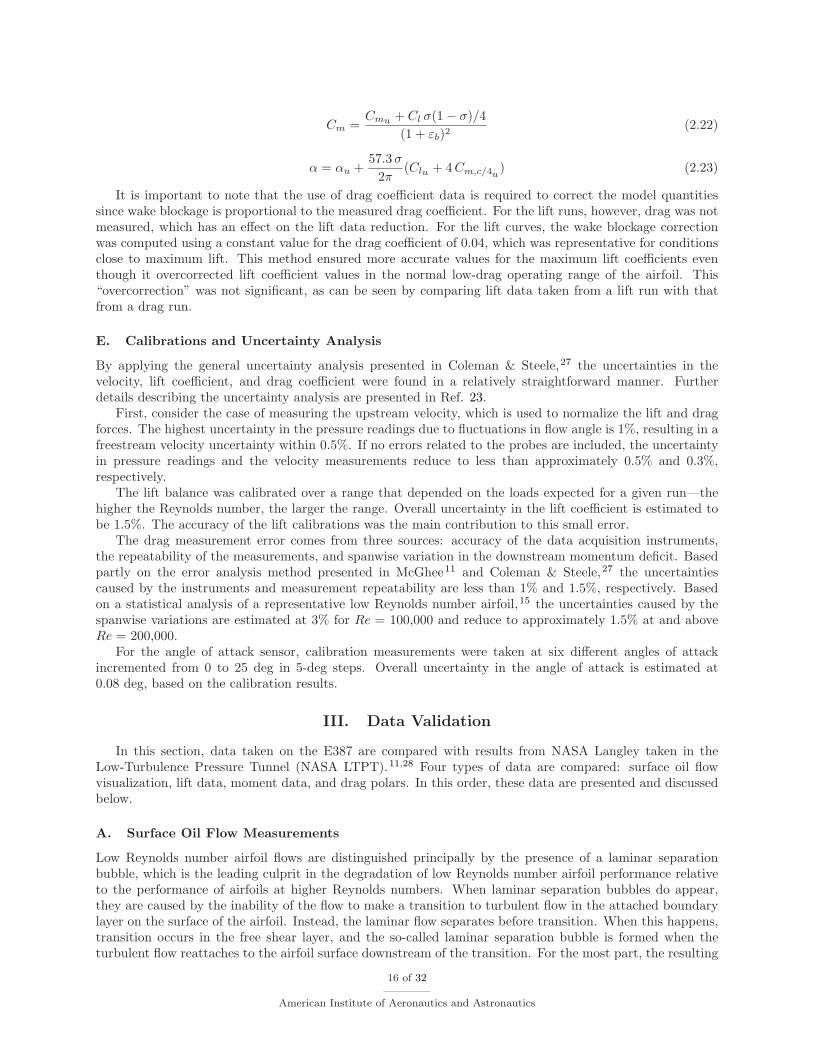
Figures 25–27 show the polars and lift characteristics for the Reynolds of 100,000, 200,000 and 300,000for the flap deflections of −15, 0, 15, 30, and 40 deg. The same data is shown in Figs. 28–31 for eachrespective flap position. The decrease in the flap effectiveness with higher flap angle is clearly seen, andthis trend is consistent with the flap-effectiveness correction factor τ found in Ref. 35. The increase in dragwith higher flap deflection is dramatic, but no benchmark data exists for comparison (not the change thescale for Cd as the drag increases). It should be noted that for high flap deflections the wake is unsteady.Under such conditions, refinements to the wake rake method could be applied if the turbulence propertiesare known.20,36 With the absence of this additional data in these tests, however, no such refinements wereapplied.

B. Flat Plate Airfoils with Serrated Leading Edges

Saw-toothed structures (serrations) on the leading edge of the flippers of some aquatic animals have beenshown to delay stall, increase maximum lift, and lower drag, and these characteristics together are believedto improve the maneuverability of the humpback whale and other aquatic animals.37–39 Mutual interest40 inthese observations led to the current experiments and some preliminary results were reported previously.41

21 of 32


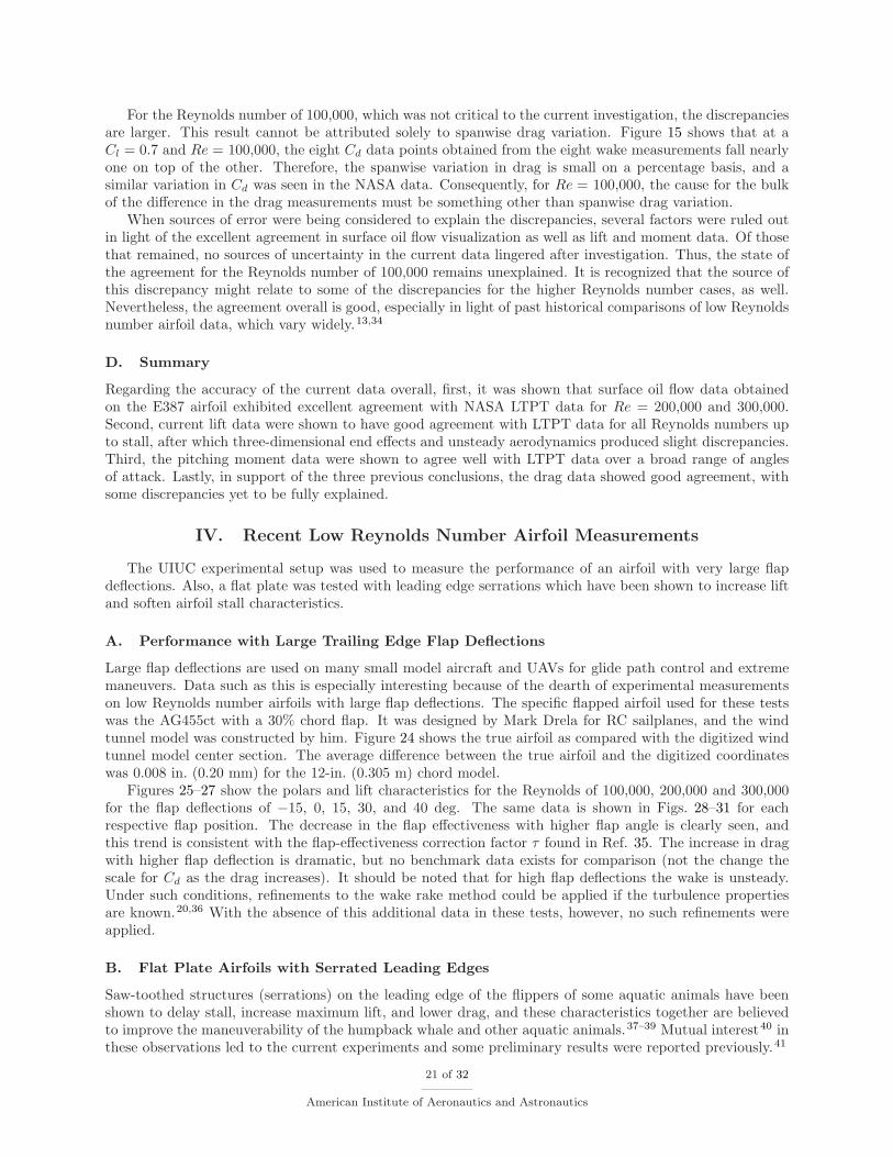
For these experiments, a flat-plate airfoil was used as the baseline, which is the airfoil configuration usedon many popular light-weight flat-foam aerobatic RC models that have become quite popular.41 The exper-iments were designed to determine if a simple serrated configuration could be used to increase performance,that is, increase lift, soften stall, and lower drag in the stall regime. The results presented here include onlylift and moment characteristics.

Four serrated leading edge configurations were tested (as well as many other configurations not reportedhere). Each had an average chord of 12 in. (0.305 m); that is, the planform area of the wind tunnel models wasthe same for each case. A given test configuration was composed of the serrated leading-edge piece attachedto a common aft flat plate. The resulting airfoil wind tunnel model was thus flat and had a serrated leadingedge. The thickness of the wind tunnel model was a uniform 3/8-in (9.52-mm) thickness or 3.125% thick(= 0.375/12).

The baseline flat-plate case is shown in Fig. 33. Figures 34–37 show the lift coefficient and momentcoefficient measurements for the four configurations at Reynolds numbers of 40,000, 80,000, and 120,000.As seen in the data, the main effect of the serrations is to smooth out the stall characteristics and momentcharacteristics relative to the baseline flat plate. The change in the moment characteristics are particularlynoteworthy because the lower pitching moment in the stalled region is suggestive of reduced separation intostall and thus lower associated drag. The results show the aerodynamics of a flat plate can be improved atlow Reynolds numbers with serrations, and the larger and more coarse serrations (case D, Fig. 37) appearto be the most favorable.

V. Conclusions

The wind tunnel test techniques described in this paper have been validated and used to test over 200airfoils at low Reynolds numbers at UIUC. The approach relies on using a force balance method for lift andmoment, and a wake rake method for airfoil drag. This paper presented new results on the AG455ct airfoilwith a large 30%-chord flap deflected over a wide range that might be used for glide path control or extrememaneuvering. In a second series of tests, a flat-plate airfoil was tested with leading edge serration geometriesto explore the effects on stall characteristics. The results support the conclusions of other researchers thatleading edge serrations (protuberances like those found on the fins/flippers of some aquatic animals) leadsto higher lift and softer stall. The results suggest that these characteristics are accompanied by lower dragin the stall and post-stall range, but drag data was not obtained in these conditions. Finally, the resultsfrom the experimental setup have been used in the design, test and validation of many airfoils used in lowReynolds number applications, and these data are readily available online and in the references providedhere (see Refs. 13–16,34).

Acknowledgments

The authors would like to thank Dr. Mark Drela of MIT for building the AG455ct flapped airfoil forthese tests. Also we thank Camille Goudeseune of the University of Illinois for design and fabrication ofconstant-area leading edges, and Upper Canada Composites (http://www.uppercanadacomposites.com/) forthe design and fabrication of flat plate wind tunnel model.

References

1“Unmanned Aircraft Systems Roadmap 2005–2030,” U.S. Department of Defense, August 2010.2“U.S. Army Unmanned Aircraft Systems Roadmap 2010–2035,” U.S. Army UAS Center of Excellence (ATZQ-CDI-C),

March 2010.3Mueller, T. J., editor, Low Reynolds Number Aerodynamics, Vol. 54 of Lecture Notes in Engineering. Springer-Verlag,

New York, June 1989.4Mueller, T. J., editor, Fixed and Flapping Wing Aerodynamics for Micro Air Vehicle ApplicationsLow Reynolds Number

Aerodynamics, Vol. 195 of Progress in Astronautics and Aeronautics. AIAA, 2001.5Pines, D. J. and Bohorquez, F., “Challenges Facing Future Micro-Air-Vehicle Development,” Journal of Aircraft , Vol. 43,

No. 2, March–Aril 2006, pp. 290–305.6Selig, M. S. and McGranahan, B. D., “Wind Tunnel Aerodynamic Tests of Six Airfoils for Use on Small Wind Turbines,”

ASME Journal of Solar Energy Engineering, Vol. 126, November 2004, pp. 986–1001.

22 of 32


7Giguere, P. and Selig, M. S., “Aerodynamic Effects of Leading-Edge Tape on Airfoils at Low Reynolds Numbers,” Wind

Energy Journal , Vol. 2, No. 3, July–September 1999, pp. 125–136.8Giguere, P. and Selig, M. S., “New Airfoils for Small Horizontal Axis Wind Turbines,” ASME Journal of Solar Energy

Engineering, Vol. 120, May 1998, pp. 108–114.9Shyy, W., Lian, Y., Tang, J., Viieru, D., and Liu, H., Aerodynamics of Low Reynolds Number Flyers, Cambridge

University Press, New York, 2008.10Mueller, T. J., “Aerodynamic Measurements at Low Reynolds Numbers for Fixed Wing Micro-Air Vehicles,” in Devel-

opment and Operation of UAVs for Military and Civil Applications, RTO AVT Course (RTO EN-9), Rhode-Saint-Genkse,Belgium, September 2006.

11McGhee, R. J., Walker, B. S., and Millard, B. F., “Experimental Results for the Eppler 387 Airfoil at Low ReynoldsNumbers in the Langley Low-Turbulence Pressure Tunnel,” NASA TM-4062, October 1988.

12Maughmer, M. D. and Bramesfeld, G., “Experimental Investigation of Gurney Flaps,” Journal of Aircraft , Vol. 45, No. 6,November–December 2008, pp. 2062–2067.

13Selig, M. S., Guglielmo, J. J., Broeren, A. P., and Giguere, P., Summary of Low-Speed Airfoil Data, Vol. 1 , SoarTechPublications, Virginia Beach, Virginia, 1995.

14Selig, M. S., Lyon, C. A., Giguere, P., Ninham, C. N., and Guglielmo, J. J., Summary of Low-Speed Airfoil Data, Vol. 2 ,SoarTech Publications, Virginia Beach, Virginia, 1996.

15Lyon, C. A., Broeren, A. P., Giguere, P., Gopalarathnam, A., and Selig, M. S., Summary of Low-Speed Airfoil Data,

Vol. 3 , SoarTech Publications, Virginia Beach, Virginia, 1997.16Selig, M. S. and McGranhan, B. D., “Wind Tunnel Aerodynamic Tests of Six Airfoils for Use on Small Wind Turbines,”

National Renewable Energy Laboratory, NREL/SR-500-35515, 2004.17Khodadoust, A., An Experimental Study of the Flowfield on a Semispan Rectangular Wing with a Simulated Glaze

Ice Accretion, Ph.D. thesis, Department of Aeronautical and Astronautical Engineering, University of Illinois at Urbana-Champaign, Illinois, 1993.

18Henze, C. M. and Bragg, M. B., “Turbulence Intensity Measurements Technique for Use in Icing Wind Tunnels,” Journal

of Aircraft , Vol. 36, No. 3, May–June 1999, pp. 577–583.19Barlow, J. B., Rae, W. H., Jr., and Pope, A., Low-Speed Wind Tunnel Testing, Third Ed., John Wiley and Sons, New

York, 1999.20Bragg, M. B. and Lu, B., “Experimental Investigation of Airfoil Drag Measurement with Simulated Leading-Edge Ice

Using the Wake Survey Method,” AIAA Paper 2000–3919, 2000.21Jones, B. M., “The Measurement of Profile Drag by the Pitot Traverse Method,” Aeronautical Research Council R&M

1688, 1936.22Schlichting, H., Boundary Layer Theory, McGraw-Hill Book Company, New York, 1979.23Guglielmo, J. J., Spanwise Variations in Profile Drag for Airfoils at Low Reynolds Numbers, Master’s thesis, Department

of Aeronautical and Astronautical, University of Illinois at Urbana-Champaign, Illinois, 1995.24Guglielmo, J. J., “Spanwise Variations in Profile Drag for Airfoils at Low Reynolds Numbers,” Journal of Aircraft ,

Vol. 33, No. 4, July–August 1996, pp. 699–707.25White, F. M., Viscous Fluid Flow , McGraw-Hill, New York, 1991.26Giguere, P. and Selig, M. S., “Freestream Velocity Corrections for Two-Dimensional Testing with Splitter Plates,” AIAA

Journal , Vol. 35, No. 7, July 1997, pp. 1195–1200.27Coleman, H. W. and W. G. Steele, Jr., Experimentation and Uncertainty Analysis For Engineers, John Wiley and Sons,

New York, 1989.28Evangleista, R., McGhee, R. J., and Walker, B. S., “Correlation of Theory to Wind-Tunnel Data at Reynolds Numbers

below 500,000,” Mueller3, pp. 131–145, pp. 131–145.29Briley, R. W. and McDonald, H., “Numerical Prediction of Incompressible Separation Bubbles,” Journal of Fluid Me-

chanics, Vol. 69, No. 4, 1975, pp. 631–656.30Davis, R. L. and Carter, J. E., “Analysis of Airfoil Transitional Separation Bubbles,” NASA CR-3791, July 1984.31Walker, G. J., Subroto, P. H., and Platzer, M. F., “Transition Modeling Effects on Viscous/Inviscid Interaction Analysis

of Low Reynolds Number Airfoil Flows Involving Laminar Separation Bubbles,” ASME Paper 88-GT-32, 1988.32Alam, M. and Sandham, N. D., “Direct Numerical Simulation of ’Short’ Laminar Separation Bubbles with Turbulent

Reattachment,” Journal of Fluid Mechanics, Vol. 403, 2000, pp. 223–250.33Lin, J. C. M. and Pauley, L. L., “Low-Reynolds-Number Separation on an Airfoil,” AIAA Journal , Vol. 34, No. 8, 1996,

pp. 1570–1577.34Selig, M. S., Donovan, J. F., and Fraser, D. B., Airfoils at Low Speeds, Soartech 8, SoarTech Publications, Virginia

Beach, Virginia, 1989.35McCormick, B. W., Aerodynamics, Aeronautics, and Flight Mechanics, John Wiley & Sons, New York, 2nd ed., 1995.36Bragg, M. B. and Lu, B., “Experimental Investigation of the Wake-Survey Method for a Bluff Body with a Highly

Turbulent Wake,” AIAA Paper 2000–3060, 2002.37Miklosovic, D. S., Murray, M. M., Howlea, L. E., and Fish, F. E., “Leading-Edge Tubercles Delay Stall on Humpback

Whale,” Physics of Fluids, Vol. 16, No. 5, May 2004, pp. L36–L42.38van Nierop, Ernst A., Alben, S., and Brenner, M. P., “How Bumps on Whale Flippers Delay Stall: An Aerodynamic

Model,” Phys. Rev. Lett., Vol. 100, No. 5, Feburary 2008, pp. 054502–1–054502–4.39Fish, F. E., Howle, L. E., and Murray, M. M., “Hydrodynamic Flow Control in Marine Mammals,” Integrative and

Comparative Biology, Vol. 48, No. 6, 2008, pp. 788–800.

23 of 32


40Goudeseune, C., Private Communications, August 2004.41Goudeseune, C., “Put Teeth on It and Take a Bite Out of your Airplane’s Stall,” Quiet Flyer , Vol. 11, No. 4, April 2006,

pp. 18–23.

24 of 32


0.00 0.01 0.02 0.03 0.04 0.05−0.5

0.0

0.5

1.0

1.5

Cd

Cl

LTPT

UIUC

E387 Re = 100,000

0.00 0.01 0.02 0.03 0.04 0.05−0.5

0.0

0.5

1.0

1.5

Cd

Cl

LTPT

UIUC

E387 Re = 200,000

0.00 0.01 0.02 0.03 0.04 0.05−0.5

0.0

0.5

1.0

1.5

Cd

Cl

LTPT

UIUC

E387 Re = 300,000

0.00 0.01 0.02 0.03 0.04 0.05−0.5

0.0

0.5

1.0

1.5

Cd

Cl

LTPT

UIUC

E387 Re = 460,000

Figure 23. Comparison between UIUC and LTPT E387 drag coefficient data for Re = 100,000, 200,000, 300,000,and 460,000.

25 of 32


figures/e387_drag_comp_100k.eps


figures/blank.eps



Diff

eren

ce (

in)

−0.03

0.00

0.03

AG455ct

Avg. Difference = 0.0080 in.

Figure 24. True AG455ct airfoil as compared with the digitized 12-in chord wind tunnel model (airfoil solidline is true, airfoil dot-dash line is measured).

0.00 0.05 0.10 0.15 0.20 0.25−0.5

0.0

0.5

1.0

1.5

2.0

Cd

Cl

"ap = −15 deg

"ap = 0 deg"ap = 15 deg

"ap = 30 deg

"ap = 40 deg

AG455ct (M. Drela)

Reynolds number = 100,000

−10 0 10 20−0.5

0.0

0.5

1.0

1.5

2.0

α (deg)

Cl

Figure 25. AG455ct airfoil polar for Re = 100,000 and flap deflections of −15, 0, 15, 30, and 40 deg.

26 of 32


figures/ag455ct_diff.eps

figuresFlap/AG455Re100k-2.eps

0.00 0.05 0.10 0.15 0.20 0.25−0.5

0.0

0.5

1.0

1.5

2.0

Cd

Cl

"ap = −15 deg


"ap = 30 deg

"ap = 40 deg

AG455ct (M. Drela)


−10 0 10 20−0.5

0.0

0.5

1.0

1.5

2.0

α (deg)

Cl


0.00 0.05 0.10 0.15 0.20 0.25−0.5

0.0

0.5

1.0

1.5

2.0

Cd

Cl

"ap = −15 deg


"ap = 30 deg

"ap = 40 deg

AG455ct (M. Drela)


−10 0 10 20−0.5

0.0

0.5

1.0

1.5

2.0

α (deg)

Cl


27 of 32




0.00 0.01 0.02 0.03 0.04 0.05−1.0

−0.5

0.0

0.5

1.0

Cd

Cl

Re = 100,000

Re = 200,000

Re = 300,000

AG455ct (M. Drela)

"ap = − 15 deg

−10 0 10 20−1.0

−0.5

0.0

0.5

1.0

1.5

α (deg)

Cl

Figure 28. AG455ct airfoil polar for flap deflection of −15 deg and Re = 100,000, 200,000 and 300,000.

0.00 0.01 0.02 0.03 0.04 0.05−0.5

0.0

0.5

1.0

1.5

Cd

Cl

Re = 100,000

Re = 200,000

Re = 300,000

AG455ct (M. Drela)

"ap = 0 deg

−10 0 10 20−0.5

0.0

0.5

1.0

1.5

2.0

α (deg)

Cl

Figure 29. AG455ct airfoil polar for flap deflection of 0 deg and Re = 100,000, 200,000 and 300,000.

28 of 32


figuresFlap/AG455N15-2.eps

figuresFlap/AG455P00-2.eps

0.00 0.01 0.02 0.03 0.04 0.05−0.5

0.0

0.5

1.0

1.5

Cd

Cl

Re = 100,000

Re = 200,000

Re = 300,000

AG455ct (M. Drela)

"ap = 15 deg

−10 0 10 20−0.5

0.0

0.5

1.0

1.5

2.0

α (deg)

Cl


0.00 0.05 0.10 0.15 0.20 0.25 0.0

0.5

1.0

1.5

2.0

Cd

Cl

Re = 100,000

Re = 200,000

Re = 300,000

AG455ct (M. Drela)

!ap = 30 deg

−10 0 10 20−0.5

0.0

0.5

1.0

1.5

2.0

α (deg)

Cl


29 of 32




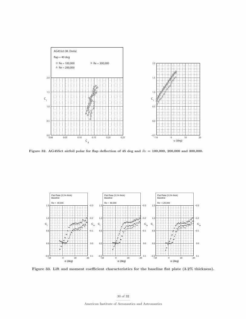
0.00 0.05 0.10 0.15 0.20 0.25 0.0

0.5

1.0

1.5

2.0

Cd

Cl

Re = 100,000

Re = 200,000

Re = 300,000

AG455ct (M. Drela)

!ap = 40 deg

−10 0 10 20−0.5

0.0

0.5

1.0

1.5

2.0

α (deg)

Cl


−10 0 10 20−0.5

0.0

0.5

1.0

1.5

α (deg)

Cl

Flat Plate (3.1% thick)Baseline

Re = 40,000

Cm

0.1

0.0

−0.1

−0.2

−0.3

−10 0 10 20−0.5

0.0

0.5

1.0

1.5

α (deg)

Cl


Re = 80,000

Cm

0.1

0.0

−0.1

−0.2

−0.3

−10 0 10 20−0.5

0.0

0.5

1.0

1.5

α (deg)

Cl


Re = 120,000

Cm

0.1

0.0

−0.1

−0.2

−0.3

Figure 33. Lift and moment coefficient characteristics for the baseline flat plate (3.2% thickness).

30 of 32



figuresFlatPlate/fp_baseline_liftcm_040_1.eps



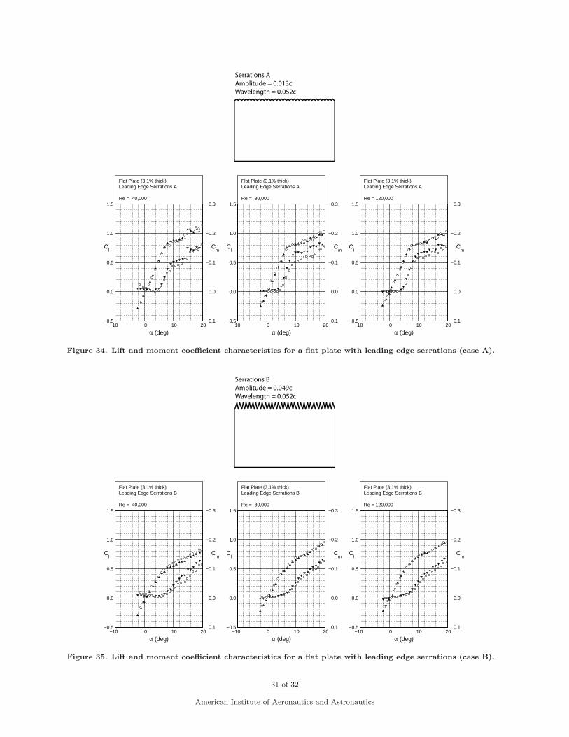
Serrations A

Amplitude = 0.013c

Wavelength = 0.052c

−10 0 10 20−0.5

0.0

0.5

1.0

1.5

α (deg)

Cl

Flat Plate (3.1% thick)Leading Edge Serrations A

Re = 40,000

Cm

0.1

0.0

−0.1

−0.2

−0.3

−10 0 10 20−0.5

0.0

0.5

1.0

1.5

α (deg)

Cl


Re = 80,000

Cm

0.1

0.0

−0.1

−0.2

−0.3

−10 0 10 20−0.5

0.0

0.5

1.0

1.5

α (deg)

Cl


Re = 120,000

Cm

0.1

0.0

−0.1

−0.2

−0.3

Figure 34. Lift and moment coefficient characteristics for a flat plate with leading edge serrations (case A).

Serrations B

Amplitude = 0.049c

Wavelength = 0.052c

−10 0 10 20−0.5

0.0

0.5

1.0

1.5

α (deg)

Cl

Flat Plate (3.1% thick)Leading Edge Serrations B

Re = 40,000

Cm

0.1

0.0

−0.1

−0.2

−0.3

−10 0 10 20−0.5

0.0

0.5

1.0

1.5

α (deg)

Cl


Re = 80,000

Cm

0.1

0.0

−0.1

−0.2

−0.3

−10 0 10 20−0.5

0.0

0.5

1.0

1.5

α (deg)

Cl


Re = 120,000

Cm

0.1

0.0

−0.1

−0.2

−0.3

Figure 35. Lift and moment coefficient characteristics for a flat plate with leading edge serrations (case B).

31 of 32


figuresFlatPlate/shark_a_was_b.eps

figuresFlatPlate/fp_shark_a_was_b_liftcm_040_1.eps



figuresFlatPlate/shark_b_was_d.eps

figuresFlatPlate/fp_shark_b_was_d_liftcm_040_1.eps



Serrations C

Amplitude = 0.013c

Wavelength = 0.125c

−10 0 10 20−0.5

0.0

0.5

1.0

1.5

α (deg)

Cl

Flat Plate (3.1% thick)Leading Edge Serrations C

Re = 40,000

Cm

0.1

0.0

−0.1

−0.2

−0.3

−10 0 10 20−0.5

0.0

0.5

1.0

1.5

α (deg)

Cl


Re = 80,000

Cm

0.1

0.0

−0.1

−0.2

−0.3

−10 0 10 20−0.5

0.0

0.5

1.0

1.5

α (deg)

Cl


Re = 120,000

Cm

0.1

0.0

−0.1

−0.2

−0.3

Figure 36. Lift and moment coefficient characteristics for a flat plate with leading edge serrations (case C).

Serrations D

Amplitude = 0.052c

Wavelength = 0.125c

−10 0 10 20−0.5

0.0

0.5

1.0

1.5

α (deg)

Cl

Flat Plate (3.1% thick)Leading Edge Serrations D

Re = 40,000

Cm

0.1

0.0

−0.1

−0.2

−0.3

−10 0 10 20−0.5

0.0

0.5

1.0

1.5

α (deg)

Cl


Re = 80,000

Cm

0.1

0.0

−0.1

−0.2

−0.3

−10 0 10 20−0.5

0.0

0.5

1.0

1.5

α (deg)

Cl


Re = 120,000

Cm

0.1

0.0

−0.1

−0.2

−0.3

Figure 37. Lift and moment coefficient characteristics for a flat plate with leading edge serrations (case D).

32 of 32


figuresFlatPlate/shark_c_was_c.eps

figuresFlatPlate/fp_shark_c_was_c_liftcm_040_1.eps



figuresFlatPlate/shark_d_was_a.eps

figuresFlatPlate/fp_shark_d_was_a_liftcm_040_1.eps



wind tunnel testing airfoils at low reynolds numbers - aerospace

Documents