wind pressure distribution on trough concentrator and...

Available online at www.sciencedirect.com

www.elsevier.com/locate/solener

ScienceDirect

Solar Energy 120 (2015) 464–478

Wind pressure distribution on trough concentrator and fluctuatingwind pressure characteristics

Qiong Zou a, Zhengnong Li a,⇑, Honghua Wu a, Rao Kuang b, Yi Hui a

a College of Civil Engineering, Hunan University, Changsha, Hunan Province 410082, Chinab Laboratory of Energy Thermal Conversion and Control of Ministry of Education, School of Energy and Environment, Southeast University, Nanjing

210096, China

Received 18 September 2014; received in revised form 13 January 2015; accepted 12 February 2015Available online 21 August 2015

Communicated by: Associate Editor Robert Pitz-Paal

Abstract

The distribution contours of mean wind pressure coefficient and fluctuating wind pressure coefficients on mirror surface under typicalworking conditions were obtained by conducting wind tunnel experiments on trough concentrator model. Meanwhile, the pattern andcharacteristics of wind pressure distribution on mirror surface were investigated; and the mean wind pressure coefficient distribution onmirror surface was studied. By focusing on fluctuating wind pressure characteristics, the factors influencing fluctuating wind pressuredistribution were analyzed, and the power spectra of fluctuating wind pressure on some measuring taps were studied. Thenon-Gaussian characteristics of the fluctuating wind pressure measured on mirror surface were also assessed on the basis of kurtosis coef-ficient and skewness coefficient.� 2015 Elsevier Ltd. All rights reserved.

Keywords: Trough concentrator; Wind tunnel experiments; Wind pressure distribution; Power spectrum; Non-Gaussian characteristics

1. Introduction

Solar thermal power is a widely discussed research topicin engineering field, and trough solar power generation(shown in Fig. 1) is an internationally dominating tech-nique with a good commercialization prospect. Since solarthermal power stations are usually located in the open, flatareas, wind load has to be properly estimated. By studyingwind pressure distribution on mirror surface of heliostatand parabolic dish collectors through boundary layer windtunnel experiment, Peterka and Derickson put forward thealgorithm of wind load design on heliostat and parabolic

http://dx.doi.org/10.1016/j.solener.2015.02.014

0038-092X/� 2015 Elsevier Ltd. All rights reserved.

⇑ Corresponding author. Tel.: +86 13974918206.E-mail address: [email protected] (Z. Li).

dish collectors (Peterka et al., 1990; Peterka andDerickson, 1992). Hosoya and Peterka have conducted aseries of wind tunnel tests. Their tests presented the peakload and the distribution of local pressure across the faceof the solar collector (Hosoya and Peterka, 2008). Theresearch of wind load on heliostat surface with differentReynolds numbers was done by Pfahl and Uhlemann(2011). Naeenia and Yaghoubi studied trough solar con-centrator by conducting numerical simulation and windtunnel experiments, and different wind loads on mirror sur-face with different pitch angles (Naeenia and Yaghoubi,2007). Gong introduced an algorithm for wind-inducedresponse calculation (Gong et al., 2012a). He also studiedthe wind load characteristics on mirror surface as well asthe characteristics of wind field around a trough concentra-tor through on-site measurement (Gong et al., 2012b).


mailto:[email protected]


http://crossmark.crossref.org/dialog/?doi=10.1016/j.solener.2015.02.014&domain=pdf

Fig. 1. Trough concentrator.

Q. Zou et al. / Solar Energy 120 (2015) 464–478 465

The trough concentrator surface is in an arch shape,thus it can be known that the wind pressure distributionon it is complex. However, there are quite a few researcheshave been done for the wind pressure distribution on suchstructures in China. And the wind resistance design oftrough concentrator in China is thus in accordance withthe existing specifications or technical standard of othercountries. However, due to different geographical featuresand climate condition, the requirements on the strengthand rigidity of the concentrator group cannot be met whiledesigned in accordance with such codes. Although therehave been some advances for trough collectors in wind tun-nel testing and in field measurement, there are still somelimiting aspects of the measurement. Compared with previ-ous wind tunnel test, in this paper, in order to obtain moreaccurate experimental data, the number of wind pressuremeasuring taps has been increased to 324. In addition, thispaper presented the distribution of fluctuating wind pres-sure on mirror surface, and checked power spectrum toexplain major influential factors on fluctuating wind pres-sure. Besides, Gaussian of wind pressure probability distri-bution was studied, and the paper presented non-Gaussianregions of mirror surface. And the value for the peak factorof non-Gaussian regions should take further research infuture. Aiming to get a precise understanding of wind loaddistribution on trough concentrator surface, wind tunnelexperiments on trough concentrator model were carriedout in HD-3 atmospheric boundary layer wind tunnel atHunan University in this study.

2. General information of the experiment

2.1. Experimental apparatus

The experiment was carried out in HD-3 atmosphericboundary layer wind tunnel in Wind Tunnel Laboratoryof Hunan University. The wind tunnel was a straight typeboundary-layer wind tunnel with low speed. The cross sec-tion of the experiment area had a width of 3 m and a heightof 2.5 m, while the stable wind speed of this wind tunnel is0.5–20 m/s. Cobra probe system was applied to measurethe instantaneous wind speed. The pressure measuring

apparatus was a DTCnet System. The DTCnet Systemhas 8 modules, and each module has 64 channels, the mea-suring range is 0.36PSI, with accuracy ±0.05%.

2.2. Experimental model

The trough concentrator prototype consists of a mirrorsurface, a supporting girder, left and right fin plates, a heatcollecting pipe bracket, a transmission system and pillarson both sides. The horizontal projection of mirror surfacewas 12.2 � 6.75 m, as shown in Fig. 2. The mirror surfaceconsisted of 96 small mirrors with a gap of 0.02–0.05 mbetween them. The length scale of the trough concentratormodel was 1:15 (Fig. 3). In order to measure the wind pres-sure on front and back mirror surface simultaneously in thepressure measuring experiment, 324 measuring taps werearranged symmetrically on both sides, with 162 taps oneach. The measuring taps on front surface were arrangedin a sequence from A to T, while the measuring taps onbackside were arranged in the sequence of AX–TX corre-sponding to the taps on front surface, as shown in Fig. 4.Since the length scale was small, the gaps between smallmirrors in the prototype were ignored in experimentalmodel.

2.3. Wind field simulation and experimental conditions

The comprehensive comparison for the near-groundwind field of wind load codes between China and Europeand America (Hong and Gu, 2004) were made, includingthe mean velocity profile and turbulence intensity profile,fluctuating wind spectrum, etc. The mean velocity profilesof Chinese and Euro codes have a faster increase thanother countries, but the mean velocity profile has little dif-ference in the codes of different countries. Compared withother countries, the turbulence intensities in Chinese codeare relatively small. For example, with terrain category B(such as the building sparse open country, suburb, forests)and at the height of 10 m, the turbulence intensity value ofChinese code is 0.12, the minimum value of the other coun-tries is 0.19, and the maximum value is 0.26.

Based on the terrain roughness characteristics of the sitewhere the trough concentrator is located, the spire-roughnesstechnique was used to simulate the atmospheric boundarylayer wind field in wind tunnel according to internationalexperiment method (Yukio, 2009) and current ChineseCode on terrain category B (Load Code for the Designof Building Structures, 2012). Wind velocity profile isexpressed by Eq. (1):

V z ¼ V bZZb

� �a

ð1Þ

where Zb is the standard reference height; Vb is the meanwind speed at the standard reference height; Z is the heightabove ground; Vz is the wind speed at the height Z; a is thesurface roughness index. The experiment in this study is to

Fig. 2. Structure of a trough concentrator.

Fig. 3. Model of a trough concentrator (1:15).Fig. 4. Layout of pressure measuring taps.

466 Q. Zou et al. / Solar Energy 120 (2015) 464–478

simulated terrain category B, so the value a was set to be0.15 accordingly.

The turbulence intensity profile is calculated accordingto Eqs. (2) and (3):

IzðzÞ ¼ I10I zðzÞ ð2Þ

IzðzÞ ¼Z10

� ��d

ð3Þ

where the turbulence intensity at the height of z is Iz; I10 isthe nominal turbulence intensity at the height of 10 m; thesurface roughness index is set as 0.14; Z is the height aboveground; d is 0.15. The wind velocity profile and turbulenceintensity profile are shown in Fig. 5. The power spectrumof longitudinal fluctuating wind speed is compared withpower spectrum by ESDU in Fig. 6.

In the wind tunnel experiment, the yaw angle of collec-tor h increases from 0� to 180� in increments of 5�. The

Fig. 5. Mean wind speed profile and the turbulence intensity profile.

Fig. 6. Wind speed power spectrum of along wind fluctuating wind.


pitch angle b increases from 0� to 90� in increments of 10�,totally it have 10 different angles. Consequently, 37 * 10 =370 operating conditions are included. The sketch map ofthe angle of mirror is shown in Fig. 7. Because the troughconcentrator is a symmetric structure along X axis and Y

axis, when the pitch angle is greater than 90�, for example,the pitch angle is 150�, and the yaw angle is 0�(150-000),

Fig. 7. Wind angles of co

the wind load of the trough solar collector of 150-000 con-dition is analogous to that of 30-180 condition. Therefore,we only measured the wind loads for the pitch angle in therange of 0–90� in wind tunnel test. (Operating condition isexpressed in the form of “pitch angle of mirror surface–yawangle”, for instance, 30-000 indicates an operating condi-tion with pitch angle of 30� and yaw angle of 0�).

3. Processing of experiment data

The measuring taps were arranged symmetrically at thesame location on the front side and back side of mirror sur-face in wind tunnel experiment, respectively. Eq. (4) is thecalculation equation of net wind pressure coefficient foreach measuring position on mirror surface:

CPiðtÞ ¼P f

i ðtÞ � P bi ðtÞ

12qV 2

H

ð4Þ

where CPi is wind pressure coefficient; i is the serial number

of measuring tap; P fi and P b

i are the wind pressures of mea-suring taps on front side and backside (the leeward sidewhen pitch angle and yaw angle are 0�). With a samplingfrequency of 312.5 Hz, 10,000 Pi data were recorded for

llector in wind tunnel.


each measuring taps. q is the air density in experiment; VH

is the wind speed of the reference tap, and the wind speed isapproximately 8.5 m/s, and the height of the referencevelocity is 0.67 m which corresponds to a prototype heightof 10 m, which is in accordance with Chinese code (LoadCode for the Design of Building Structures, 2012). By ana-lyzing CPi, the mean wind pressure coefficient, fluctuatingwind pressure coefficient could be calculated according toEqs. (5) and (6).

CPi;mean ¼1

N

XN

i¼1CPiðtÞ ð5Þ

CPi;rms ¼ffiffiffiffiffiffiffiffiffiffiffiffiffiffiffiffiffiffiffiffiffiffiffiffiffiffiffiffiffiffiffiffiffiffiffiffiffiffiffiffiffiffiffiffiffiffiffiffiffiffiffiffiffiffiffiffiffiffiffiffiffi

1

N � 1

XN

i¼1ðCPiðtÞ � CPi;meanÞ2

rð6Þ

where CPi,mean is the mean wind pressure coefficient of themeasuring tap i; CPi,rms is the fluctuating wind pressurecoefficient of the measuring tapi; Cpi is the time historyvalue of the wind pressure coefficient of a certain measur-ing tap; i = 1, 2, . . .,N, N is the number of samples.

There are several calculation method for the extremewind pressure coefficient: Peak-Factor method, RefinedPeak-Factor method, Sadek–Simiu method, Cook–Maynemethod (Davenport, 1983; Kareem and Zhao, 1994;Sadek and Simiu, 2002; Cook and Mayne, 1979, 1980).In this paper, the Peak-Factor method is adopted to getthe extreme wind pressure coefficients, which is also usedin some papers, e.g. papers (Gong et al., 2012b, 2013)and ANSI (Na, 1982). According to the analysis of Cpi,mean wind pressure coefficient CPi,mean and fluctuatingwind pressure coefficient CPi,rms, the extreme wind pressurecoefficients are as follows:

CPi;max ¼ Cpi;mean þ gCpi;rms ð7Þ

CPi;min ¼ Cpi;mean � gCpi;rms ð8Þ

where CPi,max is the peak positive wind pressure coefficient;CPi,min is the peak negative wind pressure coefficient; g isthe peak factor, with both peak positive and negative setas the same value. By checking the experiment data, itwas found that when the value of the peak factor is 3.5,guarantee rate of taps ranges from 98.2% to 99.7%. It isto say that when the peak factor is constant, the guaranteerate in different regions is inconsistent. Determine the valueof the peak factor is quite complicated for thenon-Gaussian distribution. In order to get the uniformguarantee rate on whole mirror, we can calculate the peakfactor of different positions on the mirror by the targetprobability method. The peak factor of different regionsof the mirror can take different value to improve thewind-resistant ability and make the cost more economical,this part is worthy of further investigation.

The overall loads on the solar collector are computed byintegrating the distribution of measured local pressures, asnoted by Hosoya and Peterka (2008). Because the pressuredistribution measured on the pressure model is discrete, theintegration is actually a weighted summation of pointpressures:

Q ¼XN

i¼1

wipi ð9Þ

where Q is the load effect of interest; Pi is the different pres-sure at the point i, and N is the number of pressure points.The quantity wi is the weight factor assigned at the point i.The load effect to be obtained is force, the weight factorsfor calculation of the forces in the study are tabulated areaassociated with the different pressure at the point i.

The equations of drag force coefficient and lift forcecoefficient are defined as follows:

Cfx ¼ fx12qV 2

H LWð10Þ

Cfz ¼ fz12qV 2

H LWð11Þ

where fx, fz are the wind forces along x-direction andz-direction respectively(the directions is presented inFig7); L is the span-wise length; W is the aperture widthof the collector.

4. Wind load coefficient

In this study, the wind load coefficients are calculated byintegrating the measured point pressures over the exposedarea of the solar collector. Fig8 shows wind load coefficientsfor the solar collector as a function of pitch angles obtainedby integrating the distribution of the measured load pres-sures. Fig. 8 shows wind load coefficients for the trough con-centrator as a function of pitch angles obtained by integratingthe measured point pressures over exposed area of the solarcollector concentrator and resolving the resulting load intothe specified load components. The yaw angle was 0�, andthe approach wind is perpendicular to the major axis (y axis)of the solar collector. The maximum wind drags would occurat pitch angles of 0–10�, and the minimum wind drag wouldoccur at pitch angles 90–110�. Fig. 8(b) shows that the max-imum and minimum wind lifts would be measured at pitchangles of 50� and 0�, respectively.

In comparison with the results in field measurement byGong et al. (2012b) and the results measured in wind tun-nel test by Hosoya and Peterka (2008), some suggestionswould be drawn from the analysis of Fig 8. (1) In the rangeof pitches from 0 to 180�, unfortunate pitch angles of solarcollector are 0–10� (max(fx)), 50�(max(fz)). (2) In the rangeof pitches from 0 to 180�, fortunate pitches are as follow-ing: 90–110�(min(fx)), 0� (min(fz)). (3) The trend of thevariety of wind load coefficients for the trough concentra-tor as a function of pitch angles in this paper are similarto the results of Fig. 4–4a in paper (Hosoya and Peterka,2008), besides, the maximum and minimum wind loadcoefficients also occur at the same pitch angles. However,there are some differences about drag coefficients betweenthis paper with the paper (Gong et al., 2012b) Fig. 9.These differences may be related to two reasons: Firstly,the results presented in field measurement are measured

(a) Drag coefficient as a function of pitch angles (yaw=0o)

(b) Lift coefficient as a function of pitch angles (yaw=0o)

Fig. 8. Drag coefficient cfx and lift coefficient cfz (yaw = 0�).


on two solar collectors out of eight collectors side by side,and there is a wider aperture between two collectors, whichwould cause the variation of wind load distribution.Secondly, there are differences in experimental conditions,such as the yaw angle, the flow characteristics, tap arrange-ment and tap size, other geometrical details. (4) In thispaper, the pitch angles measured were in the range of 0–90�. Actually, the trough concentrator could regulate thepitch from 0� to 360�, the deficiency about these pitchangles will be studied in the future.

5. Distribution of wind pressure

5.1. Distribution of mean wind pressure

The contour map of mean wind pressure coefficient onmirror surface in typical operating condition is shown inFig. 9.

As shown in Fig. 9, when yaw angle and pitch angle are0�, the wind pressure coefficients on mirror surface are allpositive values. The maximum value is located in the region

a little above the middle part of mirror surface. As pitchangle increases, the position of the maximum wind pressuremoves toward the edge of mirror surface in the windward.The maximum wind pressure appears at the edge as well asnear the concave tap of the mirror surface because of itsarch shape when pitch angle reaches 60�. This is differentfrom the wind pressure distribution on heliostat surface(Gong et al., 2013). Wind pressure coefficient on the lowerpart of mirror surface becomes negative when pitch anglereaches 90�. When yaw angle increases to 45�, wind pressurecoefficient starts to decrease from the edge of mirror in thewindward to the leeward along with the increase of pitchangle. When yaw angle is 90�, pitch angle variation has lit-tle influence on wind pressure coefficient distributionbecause wind direction is parallel with mirror surface.Furthermore, the wind pressure coefficient on the whole mir-ror surface is small, varying from 0.04 to 0.67. When yawangle is 135�, wind pressure coefficients on mirror surfaceare generally negative because the back side of mirror sur-face is windward, and maximum value appears at the edgeof mirror surface in the windward, and the wind pressure

(a) Operating condition 00-000 (b) Operating condition 30-000 (c) Operating condition 60-000 (d) Operating condition 90-000

(e) Operating condition 00-045 (f) Operating condition 30-045 (g) Operating condition 60-045 (h) Operating condition 90-045

(i) Operating condition 00-090 (j) Operating condition 30-090 (k) Operating condition 60-090 (l) Operating condition 90-090

(m) Operating condition 00-135 (n) Operating condition 30-135 (o) Operating condition 60-135 (p) Operating condition 90-135

(q) Operating condition 00-180 (r) Operating condition 30-180 (s) Operating condition 60-180 (t) Operating condition 90-180

Fig. 9. Contour map of mean wind pressure coefficient at the measuring taps on concentrator surface.


distribution pattern is similar to that when yaw angle is45�. When yaw angle is 180�, wind pressure coefficientsare all negative, and the maximum value appears at the

central part of mirror surface, the wind pressure distribu-tion pattern is similar to that when the yaw angle is 0�.Additionally, this paper conducts a comprehensive





(q) Operating condition 00-180 (r) Operating condition 30-180 (s) Operating condition 60-180 (t) Operating condition 90-180

Fig. 10. Contour map of fluctuating wind pressure coefficient distribution on concentrator surface.


comparison study on Fig 9 (in this paper) and Fig 11(Gong et al., 2012b). The wind distribution is different insome conditions, such as Fig. 9(g) 60-045 condition,

correspond to the pitch angle of 60� in Fig 11 (Gonget al., 2012b). The maximum wind pressure coefficientoccurs on the left edge of mirror in this paper, which


approaches the windward edge of mirror, but the maxi-mum wind pressure coefficient in Fig 11 (Gong et al.,2012b) occurs on the down edge of mirror. As can be seenfrom Fig 11 (Gong et al., 2012b), no matter how the winddirection changes, the maximum mean wind pressureappeared at the same edge, this need for further research.

5.2. Distribution of fluctuating wind pressure

The contour of fluctuating wind pressure coefficient onmirror surface under typical operating condition is shownin Fig. 10. When yaw angle is 0�, the maximum fluctuatingwind pressure coefficient moves toward the edge of mirrorsurface in the windward as pitch angle increases. This isbecause cylindrical vortex (Load Code for the Design ofBuilding Structures, 2012) forms at the edge of mirrorsurface when air flow reattaches to mirror surface as soonas it is separated by the thin mirror in the windward.Consequently, the maximum fluctuating wind pressurecoefficient appears at the edge of mirror surface. Whenpitch angle increases to 90�, besides the maximum fluctuat-ing wind pressure at the edge of mirror surface, anothertwo maximum wind pressure coefficients appear symmetri-cally in the central part of mirror surface in leeward. This isresulted from two symmetrical vortices formed in theleeward after the separation of air flow separated at theedge of mirror surface. When yaw angle increases to 45�,fluctuating wind pressure distribution shows a similarpattern despite pitch angle changes. It decreases from theedge of mirror surface in windward to leeward. Whenyaw angle is 90�, fluctuating wind pressure distributionchanges in a gradient pattern because strong air flow sepa-ration happens at the edge of mirror surface. When yawangle is 135�, the fluctuating wind pressure distribution atdifferent pitch angle is similar to the distribution of meanwind pressure. When yaw angle is 180�, the fluctuatingwind pressure distributions at pitch angle of 0�, 30� and60� are similar to the distribution of mean wind pressure;the distribution pattern at pitch angle 90� is the same asthat under the operating condition of 90-000. In general,fluctuating wind pressure distribution on mirror surface issimilar to the distribution pattern of mean wind pressure.

(a) Operating condition 00-000 (b) Operating condition 60-000 (c

Fig. 11. The maximum wind pressure coefficient on concentrator surf

5.3. Extreme wind pressure

Extreme wind pressure distribution could be derivedfrom Eqs. (7) and (8), while the maximum and minimumwind pressure coefficient distribution maps on mirror sur-face under typical operating condition and the most unfa-vorable operating condition are shown in Figs. 11 and 12,respectively. The wind pressure distribution on solar collec-tor of Fig. 11(d) 90-050 condition is corresponds to thecontour of Fig. 12(a) Gong et al., 2012b, as can be seen,the wind distribution is different, the maximum wind pres-sure coefficient occur on the left edge of mirror in thispaper, which approaches the windward edge of mirror.However, the maximum wind pressure coefficient inFig. 12(a) Gong et al., 2012b occur on the down edge ofmirror. The contour of Fig. 12(a) 00-180 condition is cor-responds to the contour of Fig. 13(c) Gong et al., 2012b,the minimum wind pressure appears at the central part ofmirror surface, which is also different with the Fig. 13(c)Gong et al., 2012b. As shown in the contour, the maximumand minimum values move to the edge of mirror surfacewith the increase of yaw angle and pitch angle; the distribu-tion pattern is similar to mean wind pressure distributionand fluctuating wind pressure distribution. High pressuresare typically concentrated around the edges of the collectorbecause of flow separation or vortex formation from thecorner where the most wind damage, such as breakage ofthe reflector panels, is expected to occur.

6. Mean wind pressure coefficient

6.1. Maximum mean wind pressure coefficient

The locations of the maximum mean wind pressure coef-ficient and the corresponding yaw angle under differentpitch angles are shown in Table 1. The mean wind pressurecoefficient in the table is the net mean wind pressurecoefficient derived by Eq. (5), while the serial numbers ofmeasuring taps on upper surface are listed in the table.As shown in the table, the maximum mean positive pres-sure appears under the operating condition with yaw angleless than 90�, where the front side of mirror is windward

) Operating condition 30-045 (d) Operating condition 90-050

ace under typical and the most unfavorable operating conditions.


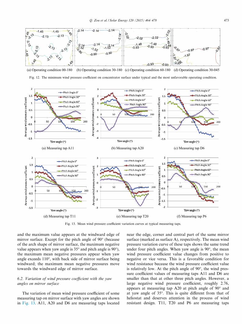
Fig. 12. The minimum wind pressure coefficient on concentrator surface under typical and the most unfavorable operating condition.

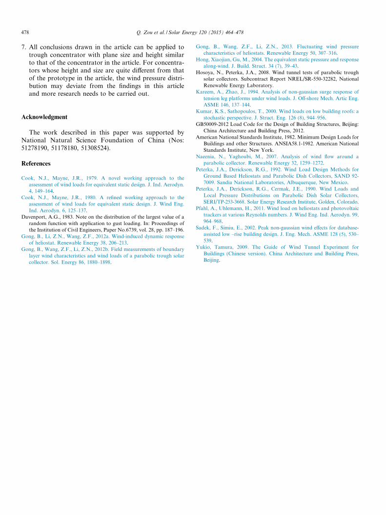
(a) Measuring tap A11 (b) Measuring tap A20 (c) Measuring tap D6

(d) Measuring tap T11 (e) Measuring tap T20 (f) Measuring tap P6

Fig. 13. Mean wind pressure coefficient variation curves at typical measuring taps.


and the maximum value appears at the windward edge ofmirror surface. Except for the pitch angle of 90� (becauseof the arch shape of mirror surface, the maximum negativevalue appears when yaw angle is 35� and pitch angle is 90�),the maximum mean negative pressures appear when yawangle exceeds 110�, with back side of mirror surface beingwindward; the maximum mean negative pressures movetowards the windward edge of mirror surface.

6.2. Variation of wind pressure coefficient with the yaw

angles on mirror surface

The variation of mean wind pressure coefficient of somemeasuring tap on mirror surface with yaw angles are shownin Fig. 13. A11, A20 and D6 are measuring taps located

near the edge, corner and central part of the same mirrorsurface (marked as surface A), respectively. The mean windpressure variation curve of these taps shows the same trendunder four pitch angles. When yaw angle is 90�, the meanwind pressure coefficient value changes from positive tonegative or vice versa. This is a favorable condition forwind resistance because the wind pressure coefficient valueis relatively low. At the pitch angle of 90�, the wind pres-sure coefficient values of measuring taps A11 and D6 aresmaller than that at other three pitch angles. However, alarge negative wind pressure coefficient, roughly 2.76,appears at measuring tap A20 at pitch angle of 90� andat yaw angle of 35�. This is quite different from that ofheliostat and deserves attention in the process of windresistant design. T11, T20 and P6 are measuring taps

Table 1Maximum mean wind pressure coefficients corresponding to different pitch angle.

Pitch angle(�)

Maximum mean wind pressure coefficient (positive) Maximum mean wind pressure coefficient (negative)

Wind pressurecoefficient

Wind angle(�)

Location of measuringpoint

Wind pressurecoefficient

Wind angle(�)

Location of measuringpoint

0 0.98 85 P11 �1.77 175 H1010 2.02 50 T21 �1.84 110 P1120 2.07 60 K2 �1.89 115 R230 2.45 45 A20 �1.93 125 R240 2.32 25 A20 �1.96 120 R250 2.00 60 K2 �1.96 125 S1160 1.98 65 K2 �2.02 125 S1170 1.72 55 K2 �2.06 130 S1180 1.67 50 M11 �2.75 150 T2090 1.05 50 N2 �2.76 35 A20


located on the same mirror surface (marked as surface B),and the mean wind pressure coefficient variation curves ofthese taps are consistent despite the change of pitch angle.With the exception of the measuring tap T20 located at thecorner, the solar collector has fortunate condition when theyaw angle is 90� and pitch angle is 90�.

Fig. 14 illustrates the variation regulations of mean pres-sure coefficients with pitch angles as a variable. In thispaper, we show 9 taps on solar collector, which correspondto taps from net-1 to net-9 in field measurement (Gonget al., 2012b). When the solar collector increase its pitchangle with respect to incoming wind, the flow separationlead to the taps the edge of mirrors have the maximumpeak pressure, and the tap B6 has the maximum peak pres-sure at pitch angle of 40�. Along with the continuous

Fig. 14. Mean pressure coefficients with

increase of pitch angle, the mean pressure coefficient valuesin most regions of mirrors turn into negative, and the tapB6 takes the minimum peak pressure at pitch angle of110–150�. There are some differences between Fig15 withFig 10 (Gong et al., 2012b), and the differences may behas the same reasons to section 4.

7. Fluctuating wind pressure characteristics

7.1. Fluctuating wind pressure power spectrum

The fluctuating wind pressure power spectra of somemeasuring taps are shown in Fig. 15 (the measuring tapsin comparison are located in the central and corner partsof the mirror surface or in the windward and leeward).

pitch angles as a variable (yaw = 0�).

(a) Operating condition 00-000

(b) Operating condition 00-090

(c) Operating condition 50-000

Fig. 15. Power spectrum of fluctuating wind pressure on mirror surface.


Reduced frequency lower than 0.1 is defined as lower fre-quency band in the article, while mid-frequency bandranges from 0.1 to 1.0 and high-frequency band refers tofrequency higher than 1.0. Under the operating condition00-000, there are a few peak values at the measuring tapsM6 and T1 in the range from 0.1 to 0.3. This is resulted

from the turbulence characteristics of fluctuating wind.Several apparent peak values are found in high frequencymeasuring tap T1 which is located at the corner of mirrorsurface and featured by complex surrounding of circlingair flow and vortex shedding. Consequently, T1 has stron-ger high-frequency components compared with measuringtap M6, and this is resulted from the vortex induced bystructural surface. Under the operating condition 00-090,peak value appears around mid-frequency band 0.3 at mea-suring tap P11 in the upstream of wind direction. Moreapparent peak values appear in mid and high-frequencybands in the downstream measuring tap P2, which showsthat most energy is concentrated in high frequency band.Under the operating condition 50-000, more high fre-quency peak values appear at downstream measuring tapS6 compared with upstream measuring tap A11.

It can be concluded from the analysis above that thepeak values appearing on fluctuating wind pressure powerspectrum of the measuring taps are related to vortex shed-ding in the area; peak values appear in lower frequencywhen the fluctuating wind power spectrum contain moreturbulence energy induced by fluctuating wind. On the con-trary, peak values appear in higher frequency when there ismore turbulence energy of vortex induced by structure sur-face at the measuring point. Besides, the scale of dominat-ing vortex acting on mirror surface changes from big scalevortex in air flow separation region at the front to smallscale vortex in reattachment region at the back. Big scalevortex is the dominant controlling energy in the separationregion in the upstream of wind direction and most peakvalues appear in mid and low-frequency band. However,high frequency energy becomes dominant as the numberof small scale vortices increases continuously at down-stream region.

7.2. Probability characteristics of fluctuating wind pressureon mirror surface

Skewness coefficient and kurtosis coefficient can be usedto test the normality of the probability distribution of windpressure. Skewness coefficient and kurtosis coefficient arecalculated by Eqs. (12) and (13), respectively:

CSk ¼XN

i¼1

½ðCPiðtÞ � CPi;meanÞ=CPi;rms�3=N ð12Þ

CKu ¼XN

i¼1

½ðCPiðtÞ � CPi;meanÞ=CPi;rms�4=N ð13Þ

All parameters in the equations are the same as that of Eqs.(5) and (6).

When CSk = 0 and CKu = 3, the distribution is regardedas normal distribution, i.e. Gaussian distribution. Skewnesscoefficient is used to test the asymmetry of data. Whenskewness coefficient CSk > 0, the distribution has positiveskewness and data on the right of mean value is more dis-persed, while data on the left of mean value is more

Table 2Skewness coefficients and kurtosis coefficients of typical measuring taps.

Operating condition A1 A11 A21 F1 F6 F11 P1 P6 P11 T1 T11 T21

00-000 CSk 0.49 0.28 0.41 0.44 0.07 0.30 0.28 �0.02 0.25 0.29 0.05 0.22CKu 3.76 3.03 3.07 3.59 2.65 3.39 3.02 2.75 3.14 2.80 2.77 2.97

00-045 CSk 0.01 0.21 0.19 0.01 0.36 0.18 �0.32 0.50 0.05 0.19 0.61 0.15CKu 3.42 2.84 3.39 3.12 2.94 3.15 3.90 3.18 3.12 3.26 3.67 2.84

00-090 CSk 0.01 �0.22 �0.58 0.03 �0.07 0.19 �0.02 �0.49 0.06 �0.09 �0.44 �0.72CKu 3.85 3.70 3.44 3.33 3.31 4.61 3.37 5.51 2.21 3.48 3.44 2.75

00-180 CSk �0.13 �0.09 �0.35 �0.24 �0.23 �0.36 �0.19 �0.11 �0.28 �0.21 �0.16 �0.39CKu 2.72 3.01 3.42 2.96 2.77 3.42 2.92 3.27 3.28 3.07 3.38 3.37

30-000 CSk 0.27 0.35 0.26 0.39 0.30 0.51 0.51 0.29 0.50 0.39 0.37 0.33CKu 3.42 2.79 3.14 3.55 2.75 3.50 3.49 3.00 3.26 3.20 3.05 3.09

30-090 CSk �0.13 �0.44 �1.05 0.03 0.02 �0.16 �0.08 �0.39 �0.16 �0.12 �0.72 �1.10CKu 3.20 4.48 4.50 3.39 3.82 2.69 3.58 3.68 2.25 3.51 4.76 4.03

60-000 CSk �0.49 �0.05 �0.68 0.31 0.26 0.37 0.48 0.27 0.50 0.39 0.28 0.46CKu 4.81 4.08 4.98 5.91 4.72 4.31 3.02 2.66 3.44 3.03 2.94 3.56

60-090 CSk �0.15 �0.20 �1.22 �0.05 �0.08 �0.47 �0.04 �0.08 �0.80 �0.08 �0.17 �1.48CKu 3.38 3.48 5.33 3.20 3.22 2.65 3.22 3.64 3.12 3.98 3.75 6.11

90-000 CSk �1.16 �0.06 �0.79 �0.45 �0.34 �0.57 0.26 0.48 0.39 �0.03 0.20 0.02CKu 8.04 3.72 4.11 4.44 3.85 4.10 2.73 3.59 2.75 3.32 3.01 2.77

90-090 CSk �0.24 �0.21 �1.28 0.01 0.12 �0.21 �0.01 0.10 �0.78 0.02 �0.07 �1.20CKu 3.44 3.61 5.02 3.18 2.89 2.31 3.22 3.35 3.25 3.48 3.42 5.52


dispersed when skewness coefficient is negative. Kurtosiscoefficient is used to test the convex degree of data distribu-tion. When kurtosis coefficient CKu > 3, represents distribu-tions sharper than the Gaussian and CKu < 3 characterizesdistributions flatter than the Gaussian. Skewness coeffi-cients CSk and kurtosis coefficients CKu of some measuringtaps are listed in Table 2, which can be used to test theGaussian characteristics of probability distribution of windpressure. A series of wind tunnel experimental study oflocal wind pressure fluctuations on low building roofs hasbeen carried out by Kumar and Sathopoulos (2000) todetermine the overall stochastic characteristics of windloads on roofs. In his study, the roof regions were consid-ered non-Gaussian distribution if the absolute values ofskewness and Kurtosis of pressure fluctuations at varioustaps are greater than 0.5 and 3.5 respectively. Gong et al.(2013) claimed in the research of heliostat that windpressure distribution does not conform to Gaussian distri-bution when kurtosis coefficient is larger than 4.0 and theabsolute value of skewness coefficient exceeds 0.5. Non-Gaussian fluctuations are generally found in flow separa-tion zones. Actually, the determination of critical valuesis just a quantitative standard for researchers to indicatenon-Gaussian fluctuations intuitively. According to thedistribution of wind pressure fluctuations and convenientdivision of non-Gaussian regions, no matter a wind pres-sure distribution follows Gaussian distribution or not, thejudgment criteria applied to heliostat is adopted becauseof the similarity between trough concentrator and heliostatin some respects.

The skewness coefficients and kurtosis coefficients ofsome measuring taps under typical operating conditionsare listed in Table 2. Both of them exceed the standardvalue of normal distribution under operating condition

90-000. For the convenience of observation, a diagram ofnon-Gaussian distribution regions of mirror surface (theregion in shadow shows non-Gaussian distribution) isgiven in Fig. 16 on the basis of data listed in Table 2.(The lower right corner region of the mirror includespoints: A1–A7, B1–B4, C1, D1–D4; the lower left cornerregion of the mirror includes points: A15–A21, B8–B11,C2, D8–D11, other regions is followed by analogy.)

It can be known intuitively from Fig. 16 that (1) exceptthe yaw angle of 90�, the wind pressure distribution of mostregion belongs to Gaussian distribution when the pitchangle is small, and non-Gaussian characteristics onlyappear in a smaller area; (2) when pitch angle of mirrorsurface is large, the wind pressure distribution on mostregions on mirror surface shows non-Gaussian characteris-tics under the operating conditions such as 60-045 or90-045, which is resulted from the separation of air flowin the direction of wind. Because of the arch shape oftrough concentrator, the wind pressure distribution on mir-ror surface in the leeward belongs to Gaussian distributionunder the operating condition 60-000 and 90-000, which isdifferent from that of heliostat with flat plane mirror(Kumar and Sathopoulos, 2000). (3) When yaw angle is90�, the wind pressure distribution on the left side of mirrorsurface approaching to incoming wind shows apparentnon-Gaussian characteristics. The explanation is thatbecause the mirror surface is parallel with wind directionand air flow is separated at edge of mirror surface in thewindward. Consequently, the wind pressure distributionon mirror surface shows non-Gaussian characteristics.From the analysis above, it can be inferred thatnon-Gaussian characteristics of wind pressure on somemeasuring taps of structural surface is resulted by vortexturbulence characteristics induced by structure surface. In





Fig. 16. Non-Gaussian regions of mirror surface.


general, wind pressure distribution on most part of mirrorsurface belongs to non-Gaussian distribution when thepitch angle of collector is large.

8. Conclusion

On the basis of pressure measuring experiment in windtunnel on trough concentrator, the conclusions below aredrawn:

1. Mean wind pressure, fluctuating wind pressure andextreme wind pressure distribution contours on mirrorsurface under typical operating conditions are presentedin the article to illustrate the pattern and characteristicsof wind pressure distribution varying with yaw angleand pitch angle. As pitch angle and yaw wind angleincrease, wind pressure distribution on mirror surfacechanges obviously, and the maximum wind pressurecoefficient moves toward the edge of mirror surface inthe windward.

2. The mean wind pressure coefficient is larger in the cor-ner of trough concentrator when pitch angle is 90�,which is different from the wind-resistant favorable con-dition of heliostat at the pitch angle of 90�. This phe-nomenon should be considered in the process of windresistant design.

3. High pressures are typically concentrated around theedges of the collector, and the breakage of the reflectorpanels at the edge is expected to occur. Therefore, themirror panels should be improved in stiffness of the edgeparts to resist wind-induced vibration.

4. In this study, when pitch angle of mirror surface is large,the wind pressure distribution on mirror surface showsnon-Gaussian characteristics. According to the non-Gaussian regions on mirror surface, the Peak-Factormethod is defective for calculating extreme pressurecoefficients. Therefore, more appropriate and conve-nient methods need to be studied in the future.

5. The wind pressure distribution pattern on mirror surfacederived from the analysis in the article can be used asreference for the optimization design of concentratorgroup and the research on mirror surface deformationcontrol.

6. Some limiting aspects of the measurement are figuredout. Firstly, pitch angle of solar collector could varyfrom 0 to 360�. In this study, pitch angles measuredare in the range of 0–90�, and these information aboutwind loads at these pitch angles will be studied in thefuture. Secondly, this study is research the isolatedcollector. Actually, in practical engineering solar collec-tors are work in groups, thus the interference effects ofneighboring collector need to be studied in the future.


7. All conclusions drawn in the article can be applied totrough concentrator with plane size and height similarto that of the concentrator in the article. For concentra-tors whose height and size are quite different from thatof the prototype in the article, the wind pressure distri-bution may deviate from the findings in this articleand more research needs to be carried out.

Acknowledgment

The work described in this paper was supported byNational Natural Science Foundation of China (Nos:51278190, 51178180, 51308524).

References

Cook, N.J., Mayne, J.R., 1979. A novel working approach to theassessment of wind loads for equivalent static design. J. Ind. Aerodyn.4, 149–164.

Cook, N.J., Mayne, J.R., 1980. A refined working approach to theassessment of wind loads for equivalent static design. J. Wind Eng.Ind. Aerodyn. 6, 125–137.

Davenport, A.G., 1983. Note on the distribution of the largest value of arandom function with application to gust loading. In: Proceedings ofthe Institution of Civil Engineers, Paper No.6739, vol. 28, pp. 187–196.

Gong, B., Li, Z.N., Wang, Z.F., 2012a. Wind-induced dynamic responseof heliostat. Renewable Energy 38, 206–213.

Gong, B., Wang, Z.F., Li, Z.N., 2012b. Field measurements of boundarylayer wind characteristics and wind loads of a parabolic trough solarcollector. Sol. Energy 86, 1880–1898.

Gong, B., Wang, Z.F., Li, Z.N., 2013. Fluctuating wind pressurecharacteristics of heliostats. Renewable Energy 50, 307–316.

Hong, Xiaojian, Gu, M., 2004. The equivalent static pressure and responsealong-wind. J. Build. Struct. 34 (7), 39–43.

Hosoya, N., Peterka, J.A., 2008. Wind tunnel tests of parabolic troughsolar collectors. Subcontract Report NREL/SR-550-32282, NationalRenewable Energy Laboratory.

Kareem, A., Zhao, J., 1994. Analysis of non-gaussian surge response oftension leg platforms under wind loads. J. Off-shore Mech. Artic Eng.ASME 146, 137–144.

Kumar, K.S., Sathopoulos, T., 2000. Wind loads on low building roofs: astochastic perspective. J. Struct. Eng. 126 (8), 944–956.

GB50009-2012 Load Code for the Design of Building Structures, Beijing:China Architecture and Building Press, 2012.

American National Standards Institute, 1982. Minimum Design Loads forBuildings and other Structures. ANSIA58.1-1982. American NationalStandards Institute, New York.

Naeenia, N., Yaghoubi, M., 2007. Analysis of wind flow around aparabolic collector. Renewable Energy 32, 1259–1272.

Peterka, J.A., Derickson, R.G., 1992. Wind Load Design Methods forGround Based Heliostats and Parabolic Dish Collectors, SAND 92-7009. Sandia National Laboratories, Albuquerque, New Mexico.

Peterka, J.A., Derickson, R.G., Cermak, J.E., 1990. Wind Loads andLocal Pressure Distributions on Parabolic Dish Solar Collectors,SERI/TP-253-3668. Solar Energy Research Institute, Golden, Colorado.

Pfahl, A., Uhlemann, H., 2011. Wind load on heliostats and photovoltaictrackers at various Reynolds numbers. J. Wind Eng. Ind. Aerodyn. 99,964–968.

Sadek, F., Simiu, E., 2002. Peak non-gaussian wind effects for database-assisted low –rise building design. J. Eng. Mech. ASME 128 (5), 530–539.

Yukio, Tamura, 2009. The Guide of Wind Tunnel Experiment forBuildings (Chinese version). China Architecture and Building Press,Beijing.

http://refhub.elsevier.com/S0038-092X(15)00084-5/h0005





































wind pressure distribution on trough concentrator and...

Documents