wind power – added value for network...
TRANSCRIPT

THESIS FOR THE DEGREE OF DOCTOR OF PHILOSOPHY
Wind Power – Added Valuefor Network Operation
NAYEEM RAHMAT ULLAH
Division of Electric Power EngineeringDepartment of Energy and Environment
CHALMERS UNIVERSITY OF TECHNOLOGYGoteborg, Sweden 2008

Wind Power – Added Value for Network OperationNAYEEM RAHMAT ULLAHISBN 978-91-7385-198-5
c© NAYEEM RAHMAT ULLAH, 2008.
Technical Report at Chalmers University of TechnologyTechnical report no. 2879ISSN 0346-718X
Division of Electric Power EngineeringDepartment of Energy and EnvironmentChalmers University of TechnologySE-412 96 GoteborgSwedenTEL: + 46 (0)31-772 1000FAX: + 46 (0)31-772 1633http://www.chalmers.se/ee/EN/
Chalmers Bibliotek, ReproserviceGoteborg, Sweden 2008

♥ To Jannatul Kawser Supti


Wind Power – Added Value for Network OperationNAYEEM RAHMAT ULLAHDivision of Electric Power EngineeringDepartment of Energy and EnvironmentChalmers University of Technology
AbstractThis dissertation deals with the investigation on different value added properties of variablespeed wind turbines (VSWT) that stem from the flexible controllability of converter inter-faced wind turbines (WT). Improvements in voltage and transient stability of a nearby grid,small-signal stability improvement on the power system, frequency control support for thenetwork operation, as well as the technical and the economic issues related to the reactivepower ancillary service provision, are among the issues covered. To demonstrate that addi-tional control functions can be incorporated in real installations, a real situation is presentedwhere the short-term voltage stability is improved as an additional feature of an existingvoltage source converter (VSC) high voltage direct current (HVDC) installation.
A finding is that the voltage and the transient stability performance of the used CigreNordic 32-bus test system during disturbances is improved when the wind farm (WF) iscomplying with the E.ON code compared to the traditional unity power factor operation.Further improvements are noticed when the example grid code is modified (increased slopeof the reactive current support line and extended reactive current support).
The damping of the inter-area mode and the local mode (where the WF is connected) ofoscillation of the studied two-area power system are increased in the presence of the WF. It isalso noticed that, the damping associated with the inter-area mode is slightly better when theconstant reactive power mode is applied compared to the voltage control mode of operation.Another finding is that the example WT exhibits a slow well damped system mode whichdepends on the WT controllers (torque and pitch controllers, and pitch compensator).
Due to the non-minimum phase characteristic of hydro dominated systems, a temporaryactive power support from WFs, utilizing the stored rotational energy in the moving turbineblades, could be helpful in reducing the network frequency fall. In this regard, it is foundthat an example WT system can provide 0.1pu extra active power support for 10s without anylarger effect on the WT operation. When this arrangement is used, both the temporary droopand the reset time of the existing speed governing system need to be reduced to maintaincertain benchmark stability properties.
From the case investigated, it is found that grid-side converters (GSC), designed to handleonly rated active power, cost around 1.5% of the total investment of the WF. However, a 50%over-rated GSC would cost around 2.25% of the total investment of the WF, and would becapable of providing 0.65 pu reactive power at the grid connection point under nominalconditions. Another finding is that higher wind speed prediction errors, i.e. a WF site witha high degree of wind variations, may result in higher payments to the WF for the reactivepower service, mainly due to the increased lost opportunity cost (LOC) component.
Keywords: variable speed wind turbine, transient stability, voltage stability, small-signalstability, frequency control, torsional oscillation, sensitivity analysis, non-minimum phasesystem, reactive power ancillary service, STATCOM, power system simulator.
iii

iv

Acknowledgements
This work has been carried out at the Division of Electric Power Engineering, Departmentof Energy and Environment at Chalmers University of Technology, Goteborg, Sweden.
The financial support provided by E.ON Sverige AB’s Research Foundation, for the lastfive years, is gratefully acknowledged. I appreciate the support from Professor Lars Sjun-nesson, Director of E.ON R&D, in this regard. I would also like to express my gratitude toDan Andersson, Ake Juntti and Christian Andersson from E.ON Elnat Sverige AB, Malmo,Dr. Jorgen Svensson from E.ON Vind Sverige AB, Malmo, Professor Olof Samuelsson fromLund University, Faculty of Engineering, Lund, all in Sweden, for their valuable technicalassistance.
I would like to take this opportunity to thank my supervisors Professor Torbjorn Thiringerand Dr. Daniel Karlsson for their kind patience, constant guidance, encouraging, stimulatingand critical comments regarding the work, and revising the thesis manuscript extensively togive it a better shape.
In addition, I acknowledge the motivational words from my examiner Professor ToreUndeland, especially when they were mostly needed.
Special thank goes to Professor Kankar Bhattacharya, who first gave me the admissioninto the Master’s Program at Chalmers, and later accepted me as a visiting student in hisresearch group at the University of Waterloo, Ontario, Canada and supervising the work forthree months. I am indebted to graduate students Jahin, Afrin, Ayed, Hemant, Steve andIsmael for helping me in so many ways in Waterloo.
I express my sincere appreciation to Professor Pablo Ledesma from Universidad CarlosIII de Madrid for his kind assistance in writing user defined models in PSS/E. Special thanksare due to Dr. Andreas Petersson, from Gothia Power AB, for providing support to comparewind farm models and giving practical tips to get started with the LaTeX.
I acknowledge the support from my fellow colleagues at the division, in particular, AbramPerdana, Marcia Martins and Julia Paixao. I also acknowledge the support from my formercolleagues, Dr. Stefan Lundberg for helping with the basics of PWM operation, Dr. JimmyEhnberg for helping with LaTeX code, and Dr. Massimo Bongiorno for tipping on Fortrancoding. Special thanks are due to Valborg Ekman and Jan-Olov Lantto for their kind support.
I would like to thank my parents and parents-in-law, and all members of my family forbelieving in me.
Last, but certainly not least, heartfelt thanks go to my wife Supti for her endless love,support and patience.
Nayeem R. UllahGoteborg, SwedenOctober 2008
v

vi

Table of Contents
Abstract iii
Acknowledgement v
Table of Contents vii
1 Introduction 11.1 Current wind power status . . . . . . . . . . . . . . . . . . . . . . . . . . 11.2 Demands from utilities on WFs . . . . . . . . . . . . . . . . . . . . . . . . 11.3 Possible interactions of WTs with the utility network . . . . . . . . . . . . 21.4 Purposes and goals . . . . . . . . . . . . . . . . . . . . . . . . . . . . . . 61.5 Contributions . . . . . . . . . . . . . . . . . . . . . . . . . . . . . . . . . 61.6 Thesis organization . . . . . . . . . . . . . . . . . . . . . . . . . . . . . . 71.7 List of publications . . . . . . . . . . . . . . . . . . . . . . . . . . . . . . 8
2 Overview of the wind energy conversion system 112.1 Aerodynamic power conversion . . . . . . . . . . . . . . . . . . . . . . . 112.2 Aerodynamic power control . . . . . . . . . . . . . . . . . . . . . . . . . 13
2.2.1 Stall control . . . . . . . . . . . . . . . . . . . . . . . . . . . . . . 142.2.2 Active stall control . . . . . . . . . . . . . . . . . . . . . . . . . . 142.2.3 Pitch control . . . . . . . . . . . . . . . . . . . . . . . . . . . . . 15
2.3 Common wind turbine generator systems . . . . . . . . . . . . . . . . . . 152.3.1 Fixed speed . . . . . . . . . . . . . . . . . . . . . . . . . . . . . . 152.3.2 Limited variable speed turbine using external rotor resistance . . . . 162.3.3 Variable speed turbine with a small scale frequency converter . . . 162.3.4 Variable speed turbine with a full scale frequency converter . . . . 17
3 Models utilized and cases studied 193.1 WT models utilized . . . . . . . . . . . . . . . . . . . . . . . . . . . . . . 19
3.1.1 Ideal current injection model . . . . . . . . . . . . . . . . . . . . . 193.1.2 Comparison of the ideal PSS/E R© model of the WF with a detail
EMTDC R© model . . . . . . . . . . . . . . . . . . . . . . . . . . 193.1.3 A market available multi-MW WT model . . . . . . . . . . . . . . 21
3.2 WT models studied in terms of functionality . . . . . . . . . . . . . . . . . 233.3 WF layout considered . . . . . . . . . . . . . . . . . . . . . . . . . . . . . 243.4 Power system models utilized . . . . . . . . . . . . . . . . . . . . . . . . . 24
3.4.1 Cigre Nordic 32-bus power system . . . . . . . . . . . . . . . . . . 24
vii

3.4.2 IEEE two-area power system . . . . . . . . . . . . . . . . . . . . . 253.4.3 Custom defined example systems . . . . . . . . . . . . . . . . . . 26
3.5 Softwares used . . . . . . . . . . . . . . . . . . . . . . . . . . . . . . . . 26
4 Voltage and transient stability improvement 274.1 Voltage stability enhancement . . . . . . . . . . . . . . . . . . . . . . . . 27
4.1.1 Steady-state voltage stability . . . . . . . . . . . . . . . . . . . . . 274.1.2 Long-term voltage stability . . . . . . . . . . . . . . . . . . . . . . 294.1.3 Short-term voltage stability . . . . . . . . . . . . . . . . . . . . . . 30
4.2 Transient stability enhancement . . . . . . . . . . . . . . . . . . . . . . . 324.3 Experimental case demonstrating improvement in
short-term voltage stability . . . . . . . . . . . . . . . . . . . . . . . . . . 334.3.1 Short description of the example . . . . . . . . . . . . . . . . . . . 334.3.2 Experimental results . . . . . . . . . . . . . . . . . . . . . . . . . 34
4.4 Grid code compliance and network stability support . . . . . . . . . . . . . 344.4.1 The fault response of a WF complying with the E.ON code . . . . . 354.4.2 Modified E.ON fault response code (modification-A) . . . . . . . . 374.4.3 Modified E.ON fault response code (modification-B) . . . . . . . . 39
5 Small-signal stability enhancement 435.1 WT model eigenvalue and sensitivity analysis . . . . . . . . . . . . . . . . 43
5.1.1 State-space model of the example WT . . . . . . . . . . . . . . . . 435.1.2 Example WT eigenvalue analysis . . . . . . . . . . . . . . . . . . 465.1.3 Parameter sensitivity analysis . . . . . . . . . . . . . . . . . . . . 49
5.2 WT dynamic interaction with the grid . . . . . . . . . . . . . . . . . . . . 535.2.1 Example WT reactive power and voltage control scheme . . . . . . 545.2.2 VSWTs with constant reactive power mode of operation . . . . . . 555.2.3 VSWTs with voltage control mode of operation . . . . . . . . . . . 595.2.4 Grid power oscillations as affected by WT control and physical pa-
rameters . . . . . . . . . . . . . . . . . . . . . . . . . . . . . . . . 615.2.5 Discussion . . . . . . . . . . . . . . . . . . . . . . . . . . . . . . 62
6 Frequency control support 656.1 Quantifying the extractable rotational energy from the turbine-generator . . 65
6.1.1 Low wind . . . . . . . . . . . . . . . . . . . . . . . . . . . . . . . 666.1.2 Medium wind . . . . . . . . . . . . . . . . . . . . . . . . . . . . . 676.1.3 High wind . . . . . . . . . . . . . . . . . . . . . . . . . . . . . . 676.1.4 Effect of WT parameters (Cp(λ), HWT ) . . . . . . . . . . . . . . . 67
6.2 Possible signal injection points for the temporaryprimary frequency control (TPFC) function . . . . . . . . . . . . . . . . . 696.2.1 Requirements on the TPFC . . . . . . . . . . . . . . . . . . . . . . 696.2.2 Low wind speed operations . . . . . . . . . . . . . . . . . . . . . 706.2.3 Disturbance rejection capability as affected by WT parameter variation 726.2.4 High wind speed operation . . . . . . . . . . . . . . . . . . . . . . 746.2.5 Gain adjustment . . . . . . . . . . . . . . . . . . . . . . . . . . . 74
6.3 Impact on the existing power system . . . . . . . . . . . . . . . . . . . . . 766.3.1 Cigre Nordic 32-bus power system for load frequency control study 76
viii

6.3.2 Wind power integration scenario . . . . . . . . . . . . . . . . . . . 776.3.3 Incoming wind power with TPFC option and its impact on the exist-
ing speed governing system . . . . . . . . . . . . . . . . . . . . . 776.3.4 Governing system parameter resetting in the presence of a WF with
the TPFC option . . . . . . . . . . . . . . . . . . . . . . . . . . . 79
7 Reactive power ancillary service provision – technical and economic issues 817.1 Reactive power capability of WFs under different grid codes . . . . . . . . 81
7.1.1 Investigated WF layout . . . . . . . . . . . . . . . . . . . . . . . . 817.1.2 Limiting factors . . . . . . . . . . . . . . . . . . . . . . . . . . . . 827.1.3 Design values . . . . . . . . . . . . . . . . . . . . . . . . . . . . . 837.1.4 WF reactive power capability considering wind variations . . . . . 83
7.2 Cost components of reactive power from a WF . . . . . . . . . . . . . . . 857.2.1 Fixed cost component . . . . . . . . . . . . . . . . . . . . . . . . 857.2.2 Cost of losses . . . . . . . . . . . . . . . . . . . . . . . . . . . . . 867.2.3 Opportunity cost component . . . . . . . . . . . . . . . . . . . . . 87
7.3 Cost model for reactive power supply from WFs . . . . . . . . . . . . . . . 897.3.1 Zero reactive power requirement from ISO . . . . . . . . . . . . . 897.3.2 A generalized structure . . . . . . . . . . . . . . . . . . . . . . . . 90
7.4 WF reactive power capability in short-term systemoperation . . . . . . . . . . . . . . . . . . . . . . . . . . . . . . . . . . . 91
8 Conclusions and future research 938.1 Future research . . . . . . . . . . . . . . . . . . . . . . . . . . . . . . . . 95
References 97
A Parameters of power systems investigated 103A.1 Two-area system data (base-case) . . . . . . . . . . . . . . . . . . . . . . . 103A.2 Custom defined systems . . . . . . . . . . . . . . . . . . . . . . . . . . . 103
A.2.1 Set-up-1 . . . . . . . . . . . . . . . . . . . . . . . . . . . . . . . . 103A.2.2 Set-up-2 . . . . . . . . . . . . . . . . . . . . . . . . . . . . . . . . 103A.2.3 Set-up-3 . . . . . . . . . . . . . . . . . . . . . . . . . . . . . . . . 103
B Parameters of wind turbine investigated 107B.1 WT parameters . . . . . . . . . . . . . . . . . . . . . . . . . . . . . . . . 107B.2 Speed controllers parameters of the WT . . . . . . . . . . . . . . . . . . . 107B.3 WT voltage controller parameters . . . . . . . . . . . . . . . . . . . . . . 108
C List of abbreviations 109
D Selected publications 111
ix

x

Chapter 1
Introduction
Wind power as an energy source has been used for a long time. Wind turbines (WT) date backmany centuries for irrigation and corn grinding. In the mid-1970s the green power activitieswere driven by the goal to reduce the dependency on fossil fuels. In today’s perspective, thegoals of the green power activities are to reduce the CO2 emission resulting from the burningof fossil fuels as well as to reduce the dependency on oil [1].
Today, the capacity of larger wind turbines has grown to 2-3MW and even higher. Someof the manufacturers have already developed prototype turbines having a rating as high as 4to 6MW [2–5].
1.1 Current wind power statusIn 2007, almost 20GW of wind power capacity was installed worldwide. In total, the world-wide installed capacity, by the end of 2007, was roughly 94GW [6].
The EU member states are leading the wind energy sector hosting 60% of the world’sinstalled wind capacity [6]. With over 56GW of installed wind power capacity by the end of2007, the production will be 119TWh of electricity in an average wind year meeting 3.7% ofthe total EU electricity demand and saving 90 million tonnes of CO2 emission annually [6].Germany, Spain and Denmark host 72% of EU’s installed wind power capacity [6].
The U.S. is hosting 17% of the world’s installed wind power capacity (16.8GW) [7].According to [6], the U.S. was the largest market for wind power in 2007 with more than5GW of new installed wind power capacity followed by Spain (3.5GW).
By the end of 2007, the total wind power capacity installed in Sweden was 788MW [6].In 2007, 217MW of new wind generation capacity was added in the generation portfolio,of which 110MW was installed offshore [6]. Several large wind farm (WF) projects, nearly2GW of installed capacity, are under planning stage which could be realized in the next 5 to10 years [8], [9].
1.2 Demands from utilities on WFsIn the past, requirements for WTs were focused mainly on protection of the turbines them-selves and did not consider the effect on the power system operation since the penetrationlevel of wind energy was fairly low. As wind energy is increasingly integrated into power
1

systems, the stability of already existing power systems is becoming a concern of utmostimportance. For example, in terms of energy penetration level, Denmark has reached thehighest level, about 20% for Jutland, followed by Germany (8%) and Spain (6%) [10]. Toensure a reliable and secure power system operation in such high penetration scenarios, theloss of a considerable part of the wind generators due to minor or medium network distur-bances cannot be accepted any more [11].
Technical regulations for WFs to be connected to a power system vary considerably fromcountry to country. The differences in requirements depend on the wind power penetrationlevel and on the robustness of the power network besides local traditional practices. Costlyand challenging requirements should only be applied if they are technically required forreliable and stable power system operation [12]. The FERC in the U. S. also suggests asystem impact study by the transmission provider before applying any costly requirementlike power factor requirement to WFs [13].
Usually fault ride-through (FRT), i.e. to stay connected to the grid during and after griddisturbances, is nowadays required by system operators, among other requirements, see forexample [14–17]. In these grid codes, it is not specified explicitly how the FRT process(active and reactive power during a network fault) should be carried out. This is clearlyspecified in the E.ON. grid code (updated April 2006) [18]. This code presents how therequirements on the reactive current support should be fulfilled during network disturbances.
In recent years, some sort of frequency response capability (capability to respond to net-work frequency deviation by altering the active power injection into the grid) is also expectedfrom WFs by the independent system operators (ISO) [15,16,18,19]. The required frequencyresponse capability varies widely among the ISOs. For example, Nordic grid operators re-quire WFs to be able to change the active power production automatically as a function ofthe network frequency [15, 19]. This requires a WF to be able to maintain a power margin,the delta regulation concept, as introduced in [15]. The German grid operator E.ON re-quires WFs to reduce their available power production when the network frequency is higherthan normal values [18]. However, WFs in the E.ON grid are currently exempted fromcontributing to the primary frequency control function, including WFs with a rated powerexceeding 100MW [18]. Hydro-Quebec, on the other hand, requires WFs (rated power ex-ceeding 10MW) to help reduce large (>0.5Hz), short-term (<10s) frequency deviation in thepower system [16]. The requirement also states that – “The frequency control system mustreduce large, short-term frequency deviations at least as much as does the inertial responseof a conventional generator whose inertia (H) equals 3.5s. This target performance is met,for instance, when the frequency control system varies the real power output dynamicallyand rapidly by about 5% for 10s when a large, short-term frequency deviation occurs in thepower system.”
Grid codes of utilities often require a WF to be able to operate continuously at the ratedvalue at a certain power factor, see [18, 19] for examples.
A comparison of some international connection regulations for WFs can be found in [20].
1.3 Possible interactions of WTs with the utility networkWind generators should preferably not degrade the stability of the existing power system,but should instead, if possible, contribute to increased system stability. For example, a focusduring the last years is the continued grid-connection of wind energy installations at certain
2

grid-voltage disturbance levels i.e. the FRT requirement. A natural next step is now to utilizethe control of active and reactive power of modern wind turbines, to further enhance theinteraction between the grid and the wind energy installation.
Today, variable speed wind turbines (VSWT) have become more common than tradi-tional fixed-speed turbines [21]. Already in 2004, the worldwide market share of VSWTswas approximately 60% [12]. The VSWTs are either of the doubly-fed induction generator(DFIG) type or the full power converter type [21]. From a power system point of view, theseconfigurations are interesting because the power electronic interface isolates the generatorcharacteristics from the rest of the power system (for the standard DFIG system, this is onlytrue for a timescale of 100ms and longer). Only the controlled converter characteristic is seenby the grid [22]. Since a variable speed wind turbine’s grid-side converter is a dc/ac voltagesource converter (VSC), it can be seen as a STATCOM (STATic synchronous COMpensator)from a hardware point of view (with limited capacity). This “wind turbine STATCOM” isalready connected to the grid, handling only active power, i.e. it transmits energy from theturbine to the grid. This means that a controlled response of active and reactive current/powerfrom WFs during network disturbances can be achieved, and this feature should accordinglybe utilized if it leads to grid stability improvements. The value of the wind farm will beincreased, if this can be done without significant additional cost. An important issue is thenthe choice and extent of control modifications.
A well known method to improve the steady-state power transmitted by the existingtransmission line and also to improve the voltage stability, is to inject reactive power into thesystem near load centers [23–25]. Power electronic based reactive power compensators likethe variable impedance type SVC (Static Var Compensator) and the converter based STAT-COM can control the voltage in a fast and continuous manner, unlike mechanically switchedcapacitors/reactors [26]. Several technical papers are available showing the applicability andeffect of these power electronic based var compensators on the voltage stability of electricpower systems [27–30]. Some utility applications of these devices are listed in [26]. Aninteresting possibility is to incorporate the STATCOM function into the control of variablespeed pitch regulated wind turbine systems which have power electronic converters alreadyincluded in their design. By doing so, this type of wind turbine system could also be seen as areactive power source like a STATCOM besides being an intermittent power source. [31,32]present real life examples where this functionality is used to improve grid stability. In addi-tion, the controlled response from a WF can also be used to improve the transient stability ofthe nearby grid.
Among the power system stability phenomena, poorly damped inter-area oscillations inthe range of 0.1Hz to 0.8Hz are a concern for the reliable operation of modern large inter-connected power systems [33]. Small-signal analysis using linear techniques is ideally suitedfor analyzing problems associated with this type of instability in power systems [24]. Thistype of study provides valuable insights into the dynamic characteristics of a power systemwhich are usually not easily evident from the time domain simulations [34]. Power systemsmall-signal stability can be improved in the presence of WTs as the converter interface de-couple the WT generator from the rest of the system [31]. Proper understanding of powersystem stability issues in the presence of present and large amount of planned future WFsare of great importance for ensuring reliable operation of the power system. This new formof generation technology and control principle associated with the market available WTs arenot as well understood as the conventional generators, by system planners [35].
3
In recent years, significant amounts of wind power have been planned to be integratedinto the existing power systems in different parts of the world. A lot of the planned WFsare at the very early stage of the planning or have just filed the connection application to theconcerned utility awaiting the grid impact/integration study [35]. From the utility planningpoint of view, system stability studies need to be done with these new technology basedgenerators, among others. For this purpose, reliable models of WTs in industry standardsimulation tools are needed, that captures the relevant power system stability issues. Unlikeconventional generators, the models of WTs are not widely standardized, which makes theanalysis of system stability in the planning stage difficult [36]. A recent effort in this regardfor the DFIG based WTs is presented in [37].
Some leading WT manufacturers (Vestas R© and GE R©) have released models of theirWTs of different series in recent years for grid studies, that have been included in industrystandard power system simulation tools like PSS/E R© [38]. The model of a multi-MW DFIGbased VSWT (3.6MW) is among the manufacturer released models. A detailed analysisof the model itself to reveal different oscillating modes, relevant for the power system sta-bility analysis, will be helpful for the understanding of converter interfaced WTs’ dynamicinteraction with the grid, as the concept penetration of the example WT is high (converterinterfaced variable speed concept). It is also important to understand the influence of allthe controllers on the WT oscillations for interconnection studies. A recent research articlepresented a modal analysis of DFIG based WT generators, which however, focused on theDFIG dynamics [39].
From a practical point of view, a comprehensive system stability analysis based on themodel of this type of WTs will help the utilities understanding the influence of converterinterfaced WTs on the system stability. It is to be noted that, as of 2004, the European marketpenetration of converter interfaced WTs was 60% [12]. The understanding thus gained canlater be utilized to analyze system stability incorporating WTs of a similar concept from otherleading manufacturers, as they are made available. A linear analysis of an example two-areapower system taking converter interfaced WTs into account has been briefly reported in [40].
The initial power surge of a hydro turbine is opposite to that desired [24]. Because of thestability reason, the temporary droop of a hydro turbine is made much larger (lower gain)than the permanent droop by utilizing a transient droop compensation function, which makesthe valve movement slower during transients [24]. The initial opposite power surge lasts for1–2s depending on the water starting time and the load step. Because of this phenomenon,during a generation deficit situation, the decelerating power (energy) is higher for a hydroturbine compared to that of a steam turbine with/without the reheat. Due to these reasons,a fast active power support for a couple of seconds following a generation deficit situation,can help a hydro dominated system in arresting the initial frequency fall.
Introducing wind power into the power system will not necessarily reduce the inertiaof the system if the control of a modern VSWT is modified, as presented in various recentreports [41–45]. The idea is to utilize the rotational energy stored in the turbine bladesto provide short term active power support. VSWTs with flexible power electronic basedcontrol systems are becoming more common today [21]. The electric power output from amodern VSWT can easily be controlled based on the network frequency and a short termnetwork frequency support can thus be provided to the grid.
It is shown in [41] that the inertia effect of a DFIG based wind turbine is not completelyhidden, rather it depends on the parameters of the rotor current controller. A slower cur-
4

rent controller facilitates inertial response from a DFIG based system, as claimed in [41].The work presented in [42] demonstrates the possibility of releasing kinetic energy from aDFIG based wind turbine system by adding an extra control loop, sensitive to the networkfrequency. The release in kinetic energy in this way is larger compared to that released froma fixed speed wind turbine system. Similar results are also presented in [43]. A quite similarconcept (an additional network frequency dependent control signal) to facilitate an inertialresponse from a DFIG based system is presented in [44] and in [45]. These recent reports( [41–45]) contributed to the development of the idea of utilizing a fraction of the rotationalenergy stored in the turbine blades for short-term active power support which could helpreducing the network frequency fall after a generation deficit situation.
Should such an untraditional frequency control support from VSWTs be realized in aregular manner, an automatic method to facilitate such a support needs to be examined,preferably on actual market available WTs, to be able to understand and estimate the effortneeded to make the necessary changes into the existing WT control system. The frequencycontrol function of the power system is solely/mainly carried out by conventional generatorsusing the speed governing system, as of today. Any untraditional way of frequency controlmeasure (temporary primary frequency control (TPFC) support from WTs, for instance),should thus be viewed from the perspective of the existing speed governing systems i.e. howthe performance and stability of the existing governing system will be affected by this typeof support. This will also help identifying potential adjustments needed, if any, to improvethe frequency governing system performance in the presence of the untraditional frequencycontrol measure from the new technology based generators.
In addition to provide active power to the grid, the wind generators with power electronicconvertors can also provide reactive power to the system by incorporating minor modifi-cations to their design and/or control architecture, as has been mentioned earlier. In theliterature, reactive power as an ancillary service has been mainly examined in the context oflarge thermal generators [46, 47] and not much work has been reported that examines howwind generators could contribute to system reactive power requirements. Reactive powerprovision from WFs is rarely procured by the ISOs. However, with increasing penetration ofwind generators into the power grid together with the increasing usage of power electronicsin turbines, WFs could be useful reactive power service providers in the future. Due to theadvancement in wind forecasting techniques in recent years, together with the power smooth-ing effect within a WF, the WFs can now be considered as a forecastable power source bythe system operators [48, 49]. Consequently, the reactive power support from the VSC ofWFs can also be treated as forecastable by the operators.
The capability curve of WFs equipped with VSWTs needs to be defined taking the windvariations into account. Different cost components associated with reactive power genera-tion by these units, need to be examined as well. A knowledge of these cost componentswill assist the ISO in formulating appropriate financial compensation mechanisms for theirreactive power service provision. When these issues are answered, WFs with reactive powercapability can be treated by the ISOs as reactive power ancillary service providers.
5

1.4 Purposes and goals
The main purpose of this thesis is to investigate different grid assisting functions utilizingconverter interfaced WTs. In particular, voltage stability, transient stability, small-signalstability and frequency control support issues, as well as, technical and economic issues ofreactive power ancillary service provision from WTs are highlighted.
A goal is to present how the implementation of an example grid code (the E.ON code)influences the stability of a nearby grid during disturbances. Moreover, a purpose is to studyand determine how an over-dimensioned converter of a wind turbine can be utilized to furtherimprove the voltage profile and transient stability of the nearby grid.
Furthermore, a purpose is to understand the nature of converter interfaced VSWTs oscil-lating modes that are of interest for power system stability studies. The goal is to analyze theimpact of the VSWTs on the power system small-signal stability.
Moreover, a goal is to examine the extent at which the existing WT control system canbe used, with minimal modifications, to facilitate the temporary extra active power supportfeature for different operating conditions. Another purpose is to identify the needed mod-ifications of the speed governing system in the presence of WFs with such untraditionalfrequency support options in a test network that resembles the Swedish/Nordic system interms of the frequency regulation system and wind power integration scenarios.
Finally, a goal is to investigate technical and economic issues related to reactive powerancillary service provision from WFs. In addition, a purpose is to consider WF sites withdifferent degrees of wind power prediction errors and its consequences on the payment toWFs for the reactive power ancillary service.
1.5 Contributions
• Development of an ideal current injection model of VSWTs: An ideal current injectionmodel of VSWTs with power electronic converters is developed for power system sta-bility studies using PSS/E. The validity of the developed ideal model is tested againsta more detailed EMTDC model (the EMTDC modeling1 was done as a part of the“Krieger’s Flak project”), and it was demonstrated that a current injection model is asufficient representation of a WF for the use in power system stability studies.
• Voltage and transient stability analysis taking WFs into account: The voltage and tran-sient stability of power systems in the presence of WFs are analyzed and quantifiedusing the industry standard simulation tool PSS/E. In addition, the stability impact ofa nearby grid of a WF is quantified when the WF complies with an example grid code,that has been updated recently (May, 2006).
• Small-signal stability analysis taking WFs into account: The small-signal stability ofan example two-area power system in the presence of a WF under various modesof operation, is determined from a comprehensive modal analysis together with thefrequency response calculations, using PSS/E.
1EMTDC modeling credit goes to Dr. Andreas Petersson from Gothia Power AB, Goteborg, Sweden.
6

• WT model eigenvalue and parameter sensitivity analysis: The nature of different os-cillating modes of a WT, i.e. the influence of different WT controllers, is identifiedfrom a detailed eigenvalue and parameter sensitivity analysis of an example WT.
• Quantification and application of temporary extra active power support: The maximumpossible temporary extra active power support, utilizing the rotational energy of theturbine blades, has been quantified taking the speed reduction possibility, accountingfor not reaching a too low rotational speed. The results are generalized by alteringvalues of the relevant parameters of the WT in a wider range from the example casevalues. Moreover, the positive effect this could have in a hydro dominated system isalso quantified.
• Proposal and evaluation of an automatic method of facilitating TPFC: The dissertationproposes a simple automatic method of facilitating the temporary additional activepower support from an actual market available multi-MW VSWT. The stability of theexisting power system speed governing system in the presence of WFs with TPFC op-tion is quantified and possible changes in the governor parameter settings are suggestedto perform the power system speed governing function satisfactorily.
• Technical and economic issues of reactive power ancillary service provision: The dis-sertation developed the model of the capability curve of a VSWT based WF withfull-scale power electronic converters taking the currently existing grid codes, and thewind variability factor into consideration. Different cost components associated withthe reactive power generation are determined and hence, the reactive power cost modelis developed. A new method for defining the lost opportunity cost (LOC) for WFs isproposed that takes the wind fluctuations into account.
1.6 Thesis organizationThe organization of the thesis is as follows:
• Chapter 2: A brief overview of aerodynamic power conversion and of common WTgenerator systems.
• Chapter 3: A summary of different investigated models used (power system models,WT models) and cases studied in this thesis.
• Chapter 4: The main results of voltage and transient stability studies including WFs.
• Chapter 5: The eigenvalue and sensitivity analysis of a WT system and the results of asmall-signal stability study including WFs.
• Chapter 6: The analysis and results of frequency control support study.
• Chapter 7: The technical and economical issues associated with reactive power ancil-lary service provision from WFs.
• Chapter 8: Conclusions and proposals for future research.
7

Appendix A gives the network data of the power systems investigated, while Appendix Bpresents the data of the example WT model considered. Appendix C presents a list of ab-breviations used in the dissertation. In Appendix D, the full papers of the IEEE Transactionspublications within this research project are reprinted.2
1.7 List of publicationsThe content of the thesis is based on the following published/submitted articles:
• N. R. Ullah, T. Thiringer, “On oscillations in power systems in the presence of vari-able speed wind turbines—Part I: wind turbine model eigenvalue and sensitivity analy-sis”, IEEE Transactions on Power Systems, submitted for publication, paper no. tpwrs-00867.2008.
• N. R. Ullah, T. Thiringer, “On oscillations in power systems in the presence of vari-able speed wind turbines—Part II: wind turbines dynamic interaction with the grid”,IEEE Transactions on Power Systems, submitted for publication, paper no. tpwrs-00869.2008.
• N. R. Ullah, T. Thiringer, “Primary frequency control support from variable speedwind turbines”, IEEE Transactions on Power Systems, submitted for publication, paperno. tpwrs-00621.2008.
• N. R. Ullah, K. Bhattacharya, T. Thiringer, “Wind farms as reactive power ancillaryservice providers – technical and economic issues”, IEEE Transactions on EnergyConversion, accepted for publication, paper no. tec-00137.2008.
• N. R. Ullah, T. Thiringer, D. Karlsson, “Temporary primary frequency control supportby variable speed wind turbines – potential and applications”, IEEE Transactions onPower Systems, vol. 23, no. 2, pp. 601-612, May 2008.
• N. R. Ullah, T. Thiringer, D. Karlsson, “Voltage and transient stability support bywind farms complying with the E.ON Netz grid code”, IEEE Transactions on PowerSystems, vol. 22, no. 4, pp. 1647-1656, Nov. 2007.
• N. R. Ullah, T. Thiringer, “Variable speed wind turbines for power system stabilityenhancement”, IEEE Transactions on Energy Conversion, vol. 22, no. 1, pp. 52-60,March 2007.
• A. Larsson, A. Petersson, N. R. Ullah, O. Carlsson, “Krieger’s Flak wind farm” inProc. Nordic Wind Power Conference (NWPC-06), Espoo, Finland, 22-23 May 2006.
During the Ph.D. project, the author has also contributed in the following reports:
• N. R. Ullah, A. Larsson, A. Petersson, D. Karlsson, “Detailed modeling for large scalewind power installations – a real project case study ”, In Proc. IEEE 3rd InternationalConference on Electric Utility Deregulation and Restructuring and Power Technolo-gies (DRPT-08), NanJing, China, 6-9 April 2008, pp. 46-56.
2 with permission from the IEEE Intellectual Property Rights Office.
8

• N. R. Ullah, T. Thiringer, “Improving voltage stability by utilizing reactive powerinjection capability of variable speed wind turbines”, International Journal of Powerand Energy Systems, vol. 28, no. 3, pp. 289-297, March 2008.
• N. R. Ullah, T. Thiringer, “Effect of operational modes of a wind farm on the transientstability of nearby generators and on power oscillations: a Nordic grid study”, WindEnergy Journal, vol. 11, no. 1, pp. 63-73, Jan./Feb. 2008.
• N. R. Ullah, J. Svensson, A. Karlsson, “Comparing the fault response between awind farm complying with the E.ON Netz code and that of classical generators”, InProc. Nordic Wind Power Conference (NWPC-07), Roskilde, Denmark, 1-2 Nov. 2007.
• N. R. Ullah, K. Bhattacharya, T. Thiringer, “Reactive power ancillary service fromwind farms”, In Proc. IEEE Electrical Power Conference (EPC-07), Montreal, Canada,25-26 Oct. 2007, pp. 562-567.
• N. R. Ullah, T. Thiringer, D. Karlsson, “Operation of wind energy installations duringpower network disturbances”, In Proc. IEEE Electric Machine and Drive Conference(IEMDC-07), Antalya, Turkey, 3-5 May 2007, pp. 1396-1400.
• O. Carlson, A. Perdana, N. R. Ullah, M. Martins and E. Agneholm, “Power systemvoltage stability related to wind power generation” in Proc. European Wind EnergyConference and Exhibition (EWEC-06), Athens, Greece, 27 Feb.-2 March 2006.
• N. R. Ullah, “Small scale integration of variable speed wind turbine into the local gridand its voltage stability aspects,” in Proc. IEEE International Conference on FuturePower Systems (FPS-05), Amsterdam, The Netherlands, 16-18 Nov. 2005.
• N. R. Ullah, T. Thiringer, “Improving voltage stability by utilizing reactive power in-jection capability of variable speed wind turbines,” in Proc. 8th IASTED InternationalConference on Power and Energy Systems (PES-05), Marina Del Rey, CA, USA, 24-26Oct. 2005.
• N. R. Ullah, J. Groot, T. Thiringer, “The use of a combined battery/supercapacitorstorage to provide voltage ride-through capability and transient stabilizing propertiesby wind turbines,” in Proc. 1st European Symposium on Super Capacitors and Appli-cations (ESSCAP-04), Belfort, France, 4-5 Nov. 2004.
• N. R. Ullah, O. Olasumbo, J. Daalder, “PMU based damping algorithm of poweroscillation by resistive load switching,” in Proc. 4th IASTED International Conferenceon Power and Energy Systems (EuroPES-04), Rhodes, Greece, 28-30 June 2004.
The IEEE Transactions papers are appended at the end of this dissertation in Appendix D.
9

10

Chapter 2
Overview of the wind energy conversionsystem
The main components of a modern wind energy conversion system (WECS) are the tower,the rotor blades and the nacelle, which accommodates the transmission mechanism, the elec-tricity generating system, the wind measuring device, and for a horizontal-axis device, theyaw systems. Switching equipments and the protection system, lines and the step-up trans-formers are also required to supply the extracted wind energy to the end users. This chapterstarts with a brief description of the aerodynamic power conversion and control principle of awind turbine. Later, some commonly used generator systems for wind turbines are discussed.
2.1 Aerodynamic power conversionAn airflow over a stationary airfoil produces two forces, a lift force perpendicular to theairflow and a drag force in the direction of the airflow, as shown in Fig. 2.1 [50], [51]. A goodlift to drag ratio requires the existence of the laminar flow over both sides of the airfoil. Whenthe airfoil is allowed to move in the direction of the lift, a relative direction of the airflow isestablished as shown in Fig. 2.1. To maintain a desired lift to drag ratio, the airfoil has to bereoriented to suit the wind situation. Important to note is that the lift force is perpendicular tothe relative incoming wind, not in the direction of the airfoil motion [50], [51]. The lift anddrag forces can be split into two components parallel and perpendicular to the undisturbedwind direction. Force FQ, perpendicular to the undisturbed wind direction is the availableforce to do the useful work. Force FT , in the direction of the undisturbed wind, is the forcethat the airfoil support should withstand [50].
One way to utilize the torque force FQ is to connect three such airfoils or blades to acentral hub and allow them to rotate around a horizontal axis. This type of arrangement isknown as horizontal-axis wind turbine (HAWT). The force FQ causes a torque that rotatesthe rotor blades and this rotational motion is utilized to drive the rotor of a generator toproduce electricity [50].
The overall performance of a wind turbine depends on the construction and the orienta-tion of the blades [50]. One important parameter is the pitch angle β, shown in Fig. 2.2. Thisis the angle between the cord line of the blade and the plane of rotation. The cord line is thestraight line connecting the leading and trailing edges of an airfoil. The pitch angle is a staticangle and depends only on the orientation of the blade. Another important parameter is the
11

Fig. 2.1: Lift and drag forces on a stationary and translating airfoil.
angle of attack γ, shown in Fig. 2.2. This is the angle between the chord line of the bladeand the relative wind direction. It is a dynamic angle, depending on both the speed of theblade and the speed of the wind [50] for a given pitch angle.
Fig. 2.2: The pitch angle β and the angle of attack γ.
The lift coefficient (cl) as a function of the angle of attack, and the drag coefficient (cd)as a function of the lift coefficient for an airfoil are shown in Fig. 2.3. A tangent throughthe origin of the cd-cl curve gives the point of maximum lift to drag ration. This maximumestablishes the best angle of the resultant aerodynamic force vector for the generation oftorque [51].
Fig. 2.3: Lift and drag coefficient of an airfoil.
The fraction of power extracted from the available power in the wind by a wind turbine isgiven by the aerodynamic efficiency coefficient Cp. The aerodynamic efficiency coefficientcan be determined either by measuring the power from the turbine or, theoretically from the
12

calculated lift and drag coefficients. The mechanical power output can be written as [50]
Pm = Cp(λ, β)(1
2ρArw
3s) (2.1)
λ =Ωrrr
ws
, (2.2)
where β is the pitch angle, λ is the tip speed ratio, ws is the wind speed, Ωr is the rotor speed(low speed side of the gear box), rr is the rotor blade length, ρ is the air density and Ar isthe area swept by the rotor. The coefficient of performance Cp is not a constant number,instead it varies with the tip speed ratio, i.e. with the wind speed, the rotational speed of theturbine and turbine blade parameters such as angle of attack and pitch angle. Typical Cp(λ)curves and typical wind speed-power curves for different pitch angles are shown in Fig. 2.4and Fig. 2.5, respectively.
2 4 6 8 10 120
0.1
0.2
0.3
0.4
Tip speed ratio (λ)
CP
02
4
68
101220
02
4
68
101220
02
4
68
101220
02
4
68
101220
02
4
68
101220
02
4
68
101220
02
4
68
101220
02
4
68
101220
02
4
68
101220
02
4
68
101220
02
4
68
101220
Fig. 2.4: Typical λ–Cp curves for different pitch angles (from 0o to 20o).
5 10 15 20 250
0.5
1
1.5
Wind speed [m/s]
P [p
u]
0
3
6
9 15 30
nominal power
0
3
6
9 15 30
nominal power
0
3
6
9 15 30
nominal power
0
3
6
9 15 30
nominal power
0
3
6
9 15 30
nominal power
0
3
6
9 15 30
nominal power
0
3
6
9 15 30
nominal power
0
3
6
9 15 30
nominal power
0
3
6
9 15 30
nominal power
0
3
6
9 15 30
nominal power
0
3
6
9 15 30
nominal power
Fig. 2.5: Typical wind speed–power curves of a wind turbine operating at a fixed speed fordifferent pitch angles.
2.2 Aerodynamic power controlThe operation of a wind turbine involves starting the wind turbine from rest, stopping theturbine under a wide range of normal and abnormal conditions and modulating the sys-
13

tem power and load while the turbine is running [52]. The starting of many stalled con-trolled wind turbines is accomplished by turning the generator by a starter motor. For pitchcontrolled turbines, the aerodynamic control surface is employed to assist the startup pro-cess [52]. Aerodynamic control is also very attractive for stopping the rotor and almost allhorizontal axis wind turbines employ some sort of aerodynamic control to prevent rotor over-speed, in particular, new large ones. The control function to regulate the output power hasbeen accomplished historically by the use of aerodynamic control surfaces [52].
The power output from a wind turbine is determined by the value of CP which dependson wind speed, turbine rotational speed and the blade pitch angle. As the speed of the windcan not be controlled, the power output from a wind turbine can only be controlled by varyingthe rotational speed and/or the pitch angle. Based on this fact, different control strategies canbe employed to regulate the output power of the turbine.
2.2.1 Stall control
When no blade pitching mechanism is available, i.e. when the pitch angle of the blade isconstant, the so-called stall control is employed to limit the power extraction. In normal op-eration, laminar flow is obtained at the rotor blades [53]. A high lift to drag ratio is achievedin partial loading ranges and thus a high degree of aerodynamic efficiency is attained [53].On the other hand, when the wind speed approaches the value at which the WT reaches itsrated power, further torque development should be avoided [53]. Increasing wind speed witha constant speed of rotation cause higher angle of attack (note Fig. 2.2) and finally leads toa turbulent flow. According to the characteristic of lift and drag coefficient as a function ofthe angle of attack, as shown in Fig. 2.3, a high angle of attack causes the lift coefficient todiminish in certain areas and the drag coefficient to increase [53]. When the turbine is underfull load and the wind speed increases to the range beyond, the turbulent flow results in alower rotor torque and a lower performance coefficient.
The main advantage with stall control is the fixed connection of the rotor blades to thehub. One drawback, however, is the maximization of the power production at a certain windspeed which is determined by the geometry of the rotor blade.
Wind turbine manufacturers like Made and Ecotecnia use this type of control method fortheir MW range turbines [21]
2.2.2 Active stall control
During high wind speed situations, when the angle of attack is higher, increasing the pitchangle during those situations will reduce the angle of attack i.e. the stall point is pushed into ahigher wind speed region (see Fig. 2.2). It is shown in Fig. 2.5 that during high wind speeds,varying the pitch angle in a narrow range ( 0o to 4o) can push the stall point actively towardsa higher wind speed. This control method is called active stall control [21].
Besides the better exploitation of the wind turbine system during high wind speed sit-uations, this pitching method makes emergency stopping and starting of the wind turbineeasier.
This control method is used for larger fixed speed turbines (up to 2.3MW). Manufacturerslike Vestas and Siemens use this type of control.
14

2.2.3 Pitch control
This control method is, in principle, same as the active stall control method. But in thismethod, the pitch angle is varied in a wider range. During high wind speed situations, theangle of attack can be maintained to a lower value by varying the pitch angle in a widerrange. In this way laminar flow over the rotor blades can be maintained for higher windspeeds and thus the thrust force can be reduced.
The advantage of this control method is the decrease in thrust force on the turbine duringhigh wind speeds, as well as, simplified starting and emergency stopping of the turbine. Onedrawback is the need of a pitching mechanism. Another drawback is the high slope of thepower curve at high wind speeds which will cause a large rotor power variation for a smallvariation in wind speed. This input power variation means that this type of turbine requiresa variable rotor speed operation.
This control method is used for larger variable speed turbines.
2.3 Common wind turbine generator systems
Some common WT generator systems are briefly described in this section.
2.3.1 Fixed speed
The rotor of a fixed speed wind turbine system operates at an almost fixed rotational speeddetermined by the frequency of the connected grid, the gear ratio and the generator design,regardless of the wind speed. In the fixed speed wind turbine system, the stator of the gen-erator is directly connected to the grid, as shown in Fig. 2.6. Since an induction generatoralways draws reactive power from the grid, a capacitor bank for reactive power compensationis used in this type of configuration [21]. The output power is limited by the aerodynamicdesign of the rotor blades in the case that the stall control method is used. This is the conven-tional concept earlier used by many Danish wind turbine manufacturers [21]. As mentionedearlier, for larger units up to 2.3MW, the control is often modified slightly using the activestall control. In order to increase the power production, the generator of some fixed-speedwind turbines has two sets of stator winding. One is used at low wind speeds and the otheris used at medium and high wind speeds. Manufacturers like Vestas, Siemens, Made andEcotecnia manufacture this type of fixed-speed wind turbine.
Capacitor bank
Gear
SCIG
Fig. 2.6: Fixed-speed wind turbine. SCIG = squirrel cage induction generator.
15

As the rotor speed is constant, the mechanical power on the generator shaft cannot bekept constant due to the variation in the wind speed. The mechanical power fluctuationdue to the wind variation will be transmitted into the electric output power. A variablespeed system, on the other hand, keeps the generator torque fairly constant by changing thegenerator speed in response to variations in the wind speed. Variations in the incoming windpower are absorbed to a fairly great extent by rotor speed changes. The aerodynamic powercontrol method almost exclusively used with a variable speed system is the pitch controlmethod [21].
2.3.2 Limited variable speed turbine using external rotor resistanceThis configuration uses a wound rotor induction generator (WRIG) (Fig 2.7) and has beenproduced by the Danish manufacturer Vestas since the mid-1990s. The generator is directlyconnected to the grid and a capacitor bank provides reactive power compensation in exactlythe same way as for a standard fixed speed system. The unique feature of this configurationis that it has a variable additional rotor resistance which can be changed by an opticallycontrolled converter mounted on the rotor shaft. This gives a small variable speed range.Typically the speed range is 0-10% above synchronous speed [21].
Gear
Capacitor bank
WRIG
Variable resistance
Fig. 2.7: Limited variable speed wind turbine. WRIG = wound rotor induction generator.
2.3.3 Variable speed turbine with a small scale frequency converterFig. 2.8 shows the variable speed wind turbine with a small scale frequency converter lo-cated in the rotor circuit, which is known as the DFIG (Doubly-Fed Induction Generator)system. In this type of configuration, the stator is directly connected to the grid while therotor windings are connected via slip rings to the converter. The frequency converter is ratedat approximately 30% of the generator power [21]. Typically, the variable speed range is-40% to +30% of the synchronous speed [21]. The converter also allows for control of thereactive power.
16

Power electronic
converter
DFIG
Gear
Fig. 2.8: Variable speed wind turbine with a doubly-fed induction generator and a partialscale frequency converter.
2.3.4 Variable speed turbine with a full scale frequency converterThis type of wind turbine concept has a full variable speed range, with the generator con-nected to the grid through a full scale power converter, as shown in Fig. 2.9. The generatorcan either be an induction machine or a synchronous machine. In case the generator is ofsynchronous type, it can be excited either electrically or by permanent magnets. The gearboxis designed so that the maximum rotor speed corresponds to the rated speed of the genera-tor. Some full scale power converter variable speed wind turbine systems have no gearbox.In those cases, a direct driven multiple pole generator with a large diameter is used. TheGerman wind turbine manufacturer Enercon is successfully manufacturing this type of windturbines [4], among others. Its worldwide market share is 14% (based on the total installedcapacity by the end of 2007) [4].
Power electronic
converterSG/IG
Gear
Fig. 2.9: Variable speed wind turbine with a full scale frequency converter. SG = syn-chronous generator, IG = induction generator.
17

18

Chapter 3
Models utilized and cases studied
Details regarding the PSS/E R© and EMTDC R© modeling of WTs presented in this chaptercan be found in
• A. Larsson, A. Petersson, N. R. Ullah, O. Carlsson, “Krieger’s Flak wind farm” inProc. Nordic Wind Power Conference (NWPC-06), Espoo, Finland, 22-23 May 2006.
3.1 WT models utilizedIn this dissertation, different WT modeling approaches are adopted. This section brieflydescribes the different modeling approaches.
3.1.1 Ideal current injection modelIn this current injection model, a variable speed wind turbine with a power electronic inter-face (a full power converter system) is considered. It is assumed that the wind turbines areequipped with a voltage dip ride-through facility and have a rapid current controller. Basedon these assumptions, the WF is modeled as a user written model in PSS/E which is a currentinjection source with the current limitation determined by the converter capacity constraint.As a very fast response can be achieved from a power electronic converter, the WF can thusbe modeled as a controlled current source with a small time constant (20ms). Ottersten etal. [54] experimentally demonstrated that a pulse-width modulated (PWM) voltage sourceconverter can respond very quickly to a voltage disturbance. Similar results are shown in [55]and in [56]. The results from these researches justify the assumption of modeling a WF as avery fast controlled current injection source. A similar approach of modeling a WF was alsoadopted in [32] and in [57]. This modeling approach is utilized in the calculation presentedin Chapter 4.
3.1.2 Comparison of the ideal PSS/E R© model of the WF with a detailEMTDC R© model
The suggested user defined PSS/E model of the variable speed wind turbine with a full scalepower electronic converter is verified against a more detailed EMTDC model where the gridside converter is modeled including the converter switching. The EMTDC modeling details
19

are presented in [57] .The EMTDC model of the wind turbine is shown in Fig. 3.1. InFig. 3.2, the response of the two wind farm models to a grid fault is presented. Voltage,active and reactive power are shown both at the transformer platform of the wind farm and atthe grid connection point. Good agreement between these two modeling approaches of theVSWT with a full scale power converter is achieved as can be noted from Fig. 3.2.
dc
t
v
P
dcv
+
-
Grid
filter Grid
Fig. 3.1: EMTDC model of the variable speed wind turbine with a full scale power electronicconverter.
Platform 33 kV Grid conn. point 138 kV
Vo
lta
ge
[pu
]
Time [s] Time [s]
Transformer
platform
PSS/E
EMTDC
Re
active
po
we
r
[pu
]A
ctive
po
we
r
[pu
]
cable
Fig. 3.2: Comparison of the simplified PSS/E model of the WECS described in subsection3.1.1 with that of the detailed EMTDC model (for the EMTDC model see Fig. 3.1).
20

3.1.3 A market available multi-MW WT modelA manufacturer released model of a multi-MW commercial VSWT (GE R© 3.6MW) is alsoused in this thesis which is adopted from [58, 59]. This modeling approach is utilized inthe calculations presented in Chapters 5 and 6. It has to be noted that, although the windturbine-generator system considered here is a DFIG type system, the control principle isquite similar with that of a full power converter type system–which can be found in [55,56],and accordingly, the models can be comparable. The block diagram of the example WTmodel is shown in Fig. 3.3. The reference speed (ωref ) is generated for maximum powertracking based on the measured electric power (Pef ) following the relationship [58, 59]
ωref = f(Pef ) = −0.67P 2ef + 1.42Pef + 0.51. (3.1)
The generated mechanical power (Pmt) is a complex function of wind speed (ws), rotor speed(ωwt) and pitch angle (β). The power coefficient (Cp) values of the turbine are fit with a fourthorder polynomial on λ (tip speed ratio) and β to obtain the mathematical representation ofthe Cp curves, which is
Cp(λ, β) = Σ4i=0Σ
4j=0αi,jβ
iλj. (3.2)
The values of the coefficient αi,j are given in [58]. The expression for λ is
λ = ωoRωwt
ws
(3.3)
where, ωwt is the rotor speed in pu, ws is the wind speed in m/s, ωo is the rotor base speed inrad/s and R is the rotor radius in meter. The WT mechanical power is calculated as
Pmt =1
2ρArw
3sCp(λ, β), (3.4)
where, ρ is the density of air and Ar is the rotor swept area. In the steady-state,
Pmt = Pe = Pef = Pwt0, (3.5)
ωwt = ωref = ωwt0, (3.6)
where, Pe is the injected electric power of the WT into the grid, Pwt0 and ωwt0 are the steady-state power (electrical or mechanical) and WT rotor speed, respectively, which depends onthe prevailing wind condition.
When the power is below 0.75pu, the speed reference is calculated by (3.1). At powerlevels above 0.75pu, the speed is maintained around 1.2pu. When the power hits the limit,the speed is controlled by the pitch controller by changing the pitch angle (β). The rotorspeed is computed from the inertia equation of the equivalent one-mass model of the turbine-generator. However, two-mass rotor data is also available for this model. More detailsregarding the modeling of the example turbines can be found in [58, 59].
The Cp curves of the turbine based on (3.2) are plotted, for two different pitch angles (β)together with the measured values as presented in [58, 59], in Fig. 3.4(a). The analytical Cp
curves match well with the measured ones, as can be seen from the figure. The power andthe rotor speed of the turbine are also calculated and are shown in Fig. 3.4(b).
The performance of the example WT system is tested against wind variations. For thispurpose, the example WT system is modeled in Simulink and a wind speed series consisting
21

Fig. 3.3: Block diagram of the example WT model adopted from [58]. Values of differentparameters are given in Appendix B.
4 6 8 10 120
0.2
0.4
(a)
λ
Cp
β = 10
β = 90
x
λopt
Cp,max
analyticalmeasured
5 10 15 200
0.5
1
(b)
wind speed [m/s]
[pu]
powerrotor speed
Fig. 3.4: (a) Analytical (based on (3.2)) and measured (as presented in [58,59]) Cp curves ofthe GE turbine for two different pitch angles (β= 1o, 9o), (b) the power and the rotor speedof the turbine as a function of wind speed.
of wind speed step, gust and ramp superimposed with random noise is fed as an input to theWT model. The performance is tested both in low and high wind speed regions. The resultsare shown in Fig. 3.5 and in Fig. 3.6. In Fig. 3.5, the variation in the electric power and in therotor speed together with the variation in the aerodynamic power are shown. Fast variationsin the aerodynamic power are not reflected in the electric power output of the WT. A similartest is also performed in high wind speed regions and the results are shown in Fig. 3.6. Thevariation in the rotor speed and in the pitch angle are shown in the figure. The WT controlsystem regulates the rotor speed around the maximum value of 1.2pu by changing the pitchangle which controls the accelerating torque of the WT. It is assumed that the electric powerof the WT is controlled firmly at 1.0pu due to the converter current limitation.
22

0 20 40 60 80 100 1206
8
10
[m/s
]
incoming wind
0 20 40 60 80 100 120
0.20.40.60.8
1
time [s]
[pu]
rotor speed
aerodynamicpower
electric power
Fig. 3.5: Example WT model functionality test in the low-wind speed region. The function-ality is tested against wind speed step, gust and ramp.
0 20 40 60 80 100 1208
1012141618
[m/s
],[o ]
incoming wind
pitch angle
0 20 40 60 80 100 1201
1.1
1.2
time [s]
[pu]
rotor speed
electric power
Fig. 3.6: Example WT model functionality test in the high-wind speed region. The function-ality is tested against wind speed step, gust and ramp.
3.2 WT models studied in terms of functionalityThree functions of wind energy converter systems are studied: A with induction generatorcharacteristics (traditional fixed-speed turbine), B with constant power factor operation, andC with variable power factor operation. B represents the standard control of a variable speedsystem and C represents a modified control of a variable speed systems. The capabilitydiagrams of the three systems are shown in Fig. 3.7.
The capability diagram of System B is shown with a bold horizontal line in Fig. 3.7’sright diagram, for the case when the unit is operating at unity power factor.
A variant of System B which incorporates additional active and reactive power controlalgorithms is defined as System C. In the case of a full power converter system, the grid-sideconverter controller is modified so the wind turbine system can inject/absorb reactive powerinto/from the grid while producing active power (vertical arrows in the capability diagramof Fig. 3.7’s right diagram), as long as the current rating of the converter is not violated(border represented by the circle). In addition, during a high wind speed situation, System Cis able to reschedule its active production, and provide emergency reactive support to thegrid (curved arrows in Fig. 3.7) when the turbine is operating at rated power.
23

PWT
QWT
Prated
Qrated
PWT
QWT
Prated
System A Systems B and C
Fig. 3.7: Capability diagram of wind turbine Systems A, B and C at nominal voltage. Thesystem B characteristic is represented by the thick line in the right diagram.
System A’s hardware set-up, shown in Fig. 3.8, is a squirrel cage induction generator(SCIG), directly grid-connected with a shunt capacitor bank.
System B’s hardware set-up (full power converter system or DFIG system equipped withvoltage dip ride- through facility) is also shown in Fig. 3.8. Provided that a DFIG system hasvoltage dip ride-through and a larger converter, its behavior is quite similar to a full powersystem [60].
Fig. 3.8: Hardware set-up of a fixed speed system, a full power converter system and a DFIGsystem. Ride-Through system is assumed but not drawn in the figure.
3.3 WF layout consideredThroughout the thesis, an aggregated model of a WF is considered which is connected to thegrid through a step-up transformer and an overhead line. The layout of WFs investigated willbe presented in respective chapters.
3.4 Power system models utilizedSeveral power system model are used in this dissertation to present different cases. Thissection gives an overview of different power system models utilized.
3.4.1 Cigre Nordic 32-bus power systemThe Cigre Nordic 32-bus test grid is widely used in this thesis. More details regardingthe test network can be found in [61, 62]. The original grid is shown in Fig. 3.9. In this
24

thesis the original grid setup has been modified to incorporate oncoming WFs, which will beintroduced in respective chapters.
G
G
G
GG
G
G
G
G
G
G
G
G
G
G
G
G
G
G
G
4071
4072
4011
4012
4021
4022
4032
4031
4042
4046
4047
4043
4044
4045
4041
4061
4062
4063
4051
G
G
G
External
North
Central
Southwest
400 kV
220 kV
130 kV
Fig. 3.9: Cigre Nordic 32-bus test system as considered in this dissertation.
3.4.2 IEEE two-area power systemThe IEEE two-area power system model is also utilized in this work for small-signal sta-bility calculations. The studied two-area system is adopted from [24] which was originallypresented in [63]. The two-area system is modeled in PSS/E using the available library mod-els. Values of different parameters of the models are listed in Appendix A.1. The two-areasystem is shown in Fig. 3.10.
25

Fig. 3.10: Studied two-area power system.
3.4.3 Custom defined example systemsFor the purpose of other stability calculations, three custom defined power system modelsare also used. The set-up will be introduced in the respective chapters.
3.5 Softwares usedThe power system stability calculations presented in this dissertation are mainly carried outusing the industry standard power system simulation tool PSS/E R© using its load flow, dy-namic and linear analysis modules. The current injection model of a WT is written as auser-defined model in Fortran R©. Calculations and results presentations are also done usingMatlab/Simulink R© and GAMS R©. The summary of the software usage is as follows:
• PSS/E: Chapter 3, 4, and 5.
• Matlab/Simulink: Chapter 3, 4, 5, 6, and 7.
• GAMS: Chapter 7.
26

Chapter 4
Voltage and transient stabilityimprovement
A complete version of the analysis and results presented in this chapter can be found in
• N. R. Ullah, T. Thiringer, D. Karlsson, “Voltage and Transient Stability Support byWind Farms Complying with the E.ON Netz Grid Code”, IEEE Transactions on PowerSystems, vol. 22, no. 4, pp. 1647-1656, Nov. 2007.
• N. R. Ullah, T. Thiringer, “Variable Speed Wind Turbines for Power System StabilityEnhancement”, IEEE Transactions on Energy Conversion, vol. 22, no. 1, pp. 52-60,March 2007.
4.1 Voltage stability enhancementThis section presents the results regarding the steady-state, long-term and short-term voltagestability improvement of power systems in the presence of VSWTs.
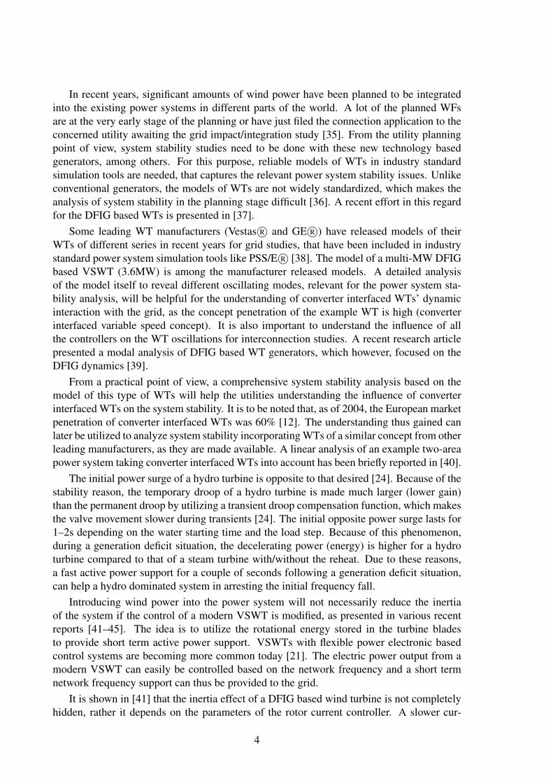
4.1.1 Steady-state voltage stabilityFig. 4.1 presents the power system set-up (set-up-1) for studying the steady state and longterm voltage stability improvement in the presence of VSWTs. Wind turbine systems A, Band C are investigated here (see Chapter 3 for the different systems). The load connectedat BUS4 is a 0.85 lagging power factor static ZIP load [25] consisting of 50% Z-load, 25%I-load and 25% P-load.
The operating point of System B during a low wind speed situation is shown in pointLW1 in Fig. 4.2, where the power factor is kept at unity. At this operating point, the windturbine does not utilize the full capacity of its power electronic converter. Keeping the activepower production at the same level, the wind turbine system can inject a substantial amountof reactive power into the grid until it reaches the operating point LW2, shown in Fig. 4.2.
Fig. 4.3 shows the PV curves or the nose curves [25], [24] at the load bus (BUS4) inthe presence of the different wind turbine systems at BUS5. It is clear from Fig. 4.3 thatthe maximum deliverable power (Pmax as defined in Fig. 4.4) is increased by using the re-active power injection facility of the variable speed System C. In other words, the voltagestability margin can be increased by reactive power injection from System C. Fig. 4.3 shows
27
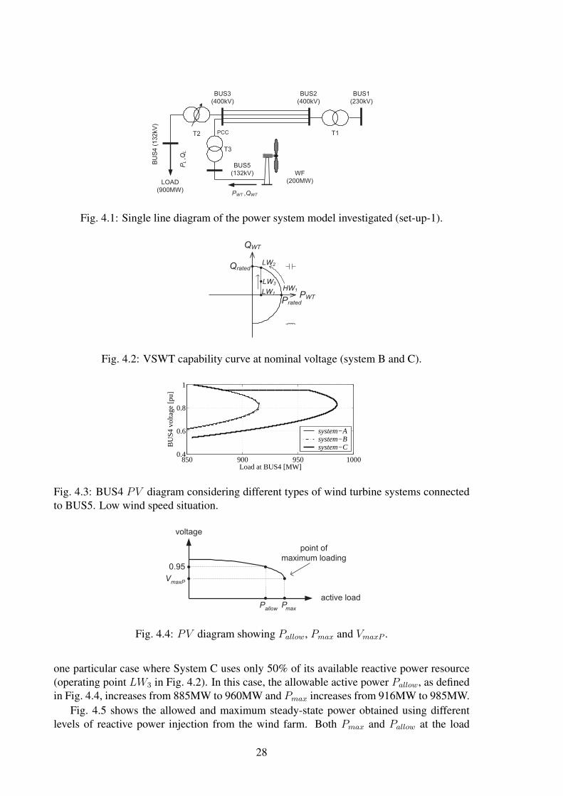
Fig. 4.1: Single line diagram of the power system model investigated (set-up-1).
QWT
PWTPrated
LW1
LW2Qrated
HW1
LW3
Fig. 4.2: VSWT capability curve at nominal voltage (system B and C).
850 900 950 10000.4
0.6
0.8
1
Load at BUS4 [MW]
BU
S4 v
olta
ge [
pu]
system−Asystem−Bsystem−C
Fig. 4.3: BUS4 PV diagram considering different types of wind turbine systems connectedto BUS5. Low wind speed situation.
voltage
active loadP
maxP
allow
VmaxP
0.95
point of
maximum loading
Fig. 4.4: PV diagram showing Pallow, Pmax and VmaxP .
one particular case where System C uses only 50% of its available reactive power resource(operating point LW3 in Fig. 4.2). In this case, the allowable active power Pallow, as definedin Fig. 4.4, increases from 885MW to 960MW and Pmax increases from 916MW to 985MW.
Fig. 4.5 shows the allowed and maximum steady-state power obtained using differentlevels of reactive power injection from the wind farm. Both Pmax and Pallow at the load
28

bus (BUS4) increase with increasing reactive power injection by the wind farm at BUS5, asexpected. It can be noted that at a higher reactive power injection level of the wind farm,the normal operating point (Pallow) progressively approaches the nose point (Pmax) of thePV curve (Fig. 4.5). More details can be found in Paper-VII, appended at the end of thisdissertation.
0 50 100 150850
900
950
1000
1050
QWT
[Mvar]
[MW
]
Pmax
Pallow
Fig. 4.5: Pmax and Pallow at BUS4 with different reactive injection levels of the wind turbinesystems. Low wind speed situation.
4.1.2 Long-term voltage stabilitySo far, results have been presented without considering the tap changing action, in orderto purely see the effect of the reactive power injection from the wind turbine. However,tap changer action is an important issue, in fact, one of the driving forces of long termvoltage instability [25], [24]. By trying to restore the load side voltage within a predefinedvoltage range, the under load tap changing transformer (ULTC) progressively degrades thetransmission level voltage which can lead to a voltage collapse. One possible way to avoidthis scenario is to utilize the reactive-power injection capability of wind turbine System C.
For this purpose, System C boosts the steady-state voltage at the connection point to thetransmission level (BUS3), within a predefined limit. Simulations are performed using thetap changing action of transformer T2 for a high load–low wind situation.
A low wind speed situation at the wind turbine installation is considered, which implies60MW (30% of the rated power) of wind power generation. The total load at the load bus(BUS4) is 910MW and 560Mvar. Now, some kind of disturbance occurs which leads tothe disconnection of one high voltage transmission line. The resulting voltage levels in thesystem are presented in Fig. 4.6. After the line disconnection, the BUS3 voltage drops dueto the increasing reactive losses in the line, and also due to the reduced line charging. Withwind turbine system A or B integrated into the power system, the transmission level voltage(BUS3) drops further due to the tap-changing action of the transformer. The tap-changingaction restores the load side voltage (BUS4), but unfortunately it has a negative impact on thegrid-side voltage and can initiate a voltage collapse event (Fig. 4.6). However, when usingSystem C, a possible voltage collapse event is avoided. In this case, the wind turbine systemutilizes its reactive power injection capability to maintain the voltage on the transmissionlevel (BUS3) within the allowed limit (±5% deviation) after the grid disturbance. Mostof the load-side voltage (BUS4) is restored by this wind farm action, and part of the load-side voltage is restored by a few transformer tap movements. Transmission level voltagereduction, due to this tap movement, is counteracted by subsequent reactive power injectionby the wind farm.
29

0 20 40 60 80 100 120
0.7
0.8
0.9
1
Time [s]
BU
S4
volta
ge [p
u]
system−Asystem−Bsystem−C
0 20 40 60 80 100 120
0.7
0.8
0.9
1
Time [s]
BU
S3
volta
ge [p
u]
0 20 40 60 80 100 120−100
0
100
200
300
400
Time [s]
QW
T [Mva
r]
Fig. 4.6: A high load - low wind situation: BUS3 and BUS4 voltage after the disconnectionof one of the transmission lines and the response of different types of wind farms to thisdisturbance.
4.1.3 Short-term voltage stability
The driving force for short-term voltage instability is the dynamic loads’ tendency to restoretheir consumed power in a one second time frame [25]. A typical load of this type is theinduction motor [25].
The impact of System C wind energy installation on short-term voltage stability, isdemonstrated using the example grid (set-up-2) shown in Fig. 4.7. Only the wind turbineSystems B and C are considered here in the short-term voltage stability study. It is assumedthat the load of: feeder-1 is a constant power load, feeder-2 is an induction motor load, andfeeder-3 is a constant impedance load. The parameters for the induction motor are chosenbased on typical values of a small industrial motor from [25] and is given in Appendix A.2.The load pf of all feeders are assumed to be 0.98 lagging.
Fig. 4.7: Single line diagram of the investigated power system (set-up-2).
30

In the calculation, a high wind speed - high load demand situation is considered. De-pending on the wind turbine technology utilized, two different cases are investigated. Theyare:
case-1: All wind turbines connected at the substation are of System B type, i.e. producingactive power at unity pf.
case-2: All wind turbines connected at the substation are of System C type.
To avoid short-term voltage instability caused by dynamic loads (induction motors, etc.),and to restore the power consumption within one or two seconds, it is necessary to providefast reactive power support near the load center [25]. The reactive support should restorea stable equilibrium point under the worst considered contingency, and should act quicklyenough before the motor slip exceeds the stall point. The short-term voltage instability mech-anism investigated here is due to a short circuit event in the network.
A three phase short-circuit fault (354ms duration) is applied in feeder-3 at location F asshown in Fig. 4.7. When all wind turbines are of System B type (case-1), after the fault-clearing (tripping the faulted feeder), the motor slip exceeds the post disturbance unstableequilibrium value and cannot reaccelerate even after the fault is cleared (see Fig. 4.8). Thevoltage at bus-5 is also shown in the figure. The bus-5 voltage is reduced to around 0.2puduring the fault.
0 0.5 1 1.5 2 2.5 3 3.5 4
−0.25
−0.2
−0.15
−0.1
−0.05
Time [s]
mot
or s
peed
dev
iatio
n [p
u]
case−1case−2
0 0.5 1 1.5 2 2.5 3 3.5 40.2
0.4
0.6
0.8
1
Time [s]
bus−
5 vo
ltage
[pu]
Fig. 4.8: Motor speed deviation and bus-5 voltage for different cases.
In the second case, where all WTs are assumed to be of System C type, the motor decel-eration is further reduced, and, after fault-clearing, the motor load accelerates and reaches itspost disturbance equilibrium point in 2.5s.
The critical fault clearing time (tcritical) [25], [24] for a three-phase-to-ground short-circuit fault applied at location F in feeder-3, is 354ms when all WECS are of System Btype. It increases to 390ms when all WECS are of System C type. More details can be foundin Paper-VII, appended at the end of this dissertation.
31

4.2 Transient stability enhancementThe transient stability improvement that can be obtained by using an appropriately chosenwind power installation control is studied using the set-up presented in Fig. 4.9 (set-up-3).A three-phase-to-ground fault (200ms duration) is applied at the middle of the line (F). Thegenerator rotor angle and the grid power (Pgrid) are studied in the presence of different typesof WTs.
Fig. 4.9: Layout of the investigated power system with a WF (set-up-3).
Fig. 4.10 shows the generator rotor angle swing, when a three-phase-to-ground fault isapplied at location F for 200ms, in the presence of Systems B and C. The generator maximumrotor angle swing is 109o when a nearby connected WT is a System B. The maximum rotorangle swing is reduced to 96o when the connected WT is a System C. When subjected to agrid fault, the reduced maximum rotor angle swing of a hydro generator, in the presence ofa nearby System C WT shows the transient stability enhancing property of System C. Theactive power production from the generator is also shown in the figure in the presence of thedifferent WTs.
0.8 1 1.2 1.4 1.6 1.8
0
50
100
Time [s]
Rot
or a
ngle
[D
egre
e]
System BSystem C
0.8 1 1.2 1.4 1.6 1.8
0
50
100
Time [s]
Gen
erat
or p
ower
[M
W]
Fig. 4.10: Generator rotor angle swing and power in the presence of different types of WECS.
When the fault is applied at F, the critical fault-clearing time is calculated in the presenceof different WTs. The critical fault-clearing time is 252ms when a System B WT is connectednear the generator, i.e. if a solid three-phase-to-ground fault at F exists longer than 252ms, thegenerator will loose its synchronism. When the nearby WT is a System C WT, the critical
32

fault-clearing time increases to 292ms, which demonstrates System C’s transient stabilityenhancing property. A detailed analysis can be found in Paper-VII, appended at the end ofthis dissertation.
4.3 Experimental case demonstrating improvement inshort-term voltage stability
In this section, a real life example is presented where the control of an existing HVDCinstallation is altered to incorporate a grid stabilizing function.
4.3.1 Short description of the example
The island of Gotland is located in the Baltic Sea, between Sweden and the Baltic states.Nasudden, a peninsula located on the southwestern part of Gotland, was previously con-nected to the main Gotland 70kV grid via a 30kV line from the northeast, but due to theincreasing installed wind energy, the transmission capacity needed to be increased. The ra-tio of the grid short-circuit capacity to the installed wind power capacity was 3, which isa very low value. After considering various alternatives, a parallel HVDC line was built,using VSC (Voltage Source Converter) technology, which provides other benefits apart frompurely transmitting energy, e.g. voltage control. More information about this installation canbe found in [64].
In Fig. 4.11 the local grid structure is presented. The DC-power from the HVDC-Lighttransmission is transformed to AC, or the other way around at this HVDC station.
10 x
L444
30 kV
10 kV
70 kV
10 kV
Measurement
point
Visby 70 kV
690 V
80 kV dc
70 kV
Substation
30 kV
Fig. 4.11: Schematic sketch of the Nasudden grid, with the Nas 1 substation.
33

4.3.2 Experimental resultsThe HVDC-Light installation is equipped with an algorithm that reduces voltage fluctua-tions and the flicker level on the 30 and 10kV side of the three-winding transformer. Thisalgorithm was tested by suddenly blocking the HVDC-Light converter. The resulting timetrace can be seen in Fig. 4.12. It is clear that the voltage starts to oscillate more after theHVDC-Light converter station is blocked. A frequency analysis verifies the observation, ascan be noted in Fig. 4.13. In this figure it can be observed that the HVDC-Light convertervastly improves the voltage level stability in a frequency range lower than 3-4Hz.
This real-life example demonstrates that “grid reinforcing functions” can be implementedto control the VSC of modern variable speed wind turbine systems.
0 50 100 15010.75
10.8
10.85
10.9
10.95
time [s]
U10
(kV
)
Fig. 4.12: Voltage on the 10kV side when the HVDC-Light converter is blocked.
10−1
100
101
102
103
104
105
Frequency [Hz]
Mag
nitu
de (
V)
Without VSC assistance
With VSC assistance
Fig. 4.13: Comparison of spectra before and after the HVDC-Light converter is blocked.
4.4 Grid code compliance and network stability support1In this section, the impact of the response of WFs during disturbances, while complyingwith an example grid code, on the stability of the nearby grid, is presented. Such an investi-gation can give insight into the possibilities of achieving improved grid performance supportfrom modern wind turbines while complying with the grid codes.
1A detailed version of the results and analysis presented in this section can be found in Paper-VI appendedat the end of this dissertation.
34

The Cigre Nordic 32-bus test network is used in this investigation. A detailed descriptionof this network can be found in [61, 62]. The original model was modified and is shownin Fig. 4.14. The main modifications made are: 1) splitting the existing transmission linesbetween buses 1044 and 1042 into three parallel lines and 2) addition of a 300MW offshoreWF at bus 1042 with two sea cables and two transformers.
Fig. 4.14: Slightly modified Cigre Nordic 32-bus grid augmented with a WF.
The WF is modeled as a controlled current source with converter current limitation (themodeling approach is described in Chapter 3).
4.4.1 The fault response of a WF complying with the E.ON codeThe E.ON fault response code
The FRT requirement for E.ON Netz is shown in Fig. 4.15. It requires a WF to be gridconnected as long as the voltage at the grid connection point is above the solid line ofFig. 4.15(a). Reactive current support should be provided on the low voltage side of thegenerator transformer following the characteristic shown in Fig. 4.15(b). It specifies the re-active current output from the WF to increase 2% (on a pu base) for a 1% voltage decrease,to have the 100% rated capacity of the converter utilized at 50% voltage at the wind turbineterminal. Accordingly, the slope of the reactive current support line, m, is 2. The E.ON
35

regulation requires WFs to provide this reactive current support within 20ms after a faultdetection. The regulation also states that if the generators are too far away from the grid con-nection point resulting in an ineffective voltage support, then the measurement of the voltagedip should be done at the grid connection point and the voltage support should be providedat this point as a function of this measured value.
Fig. 4.15: The E.ON (a) voltage limit curve at the grid connection point during a fault and(b) the reactive power support required during a network fault.
Besides providing the necessary reactive power support to the grid according to the gridcode, VSWTs can be equipped with larger converters to increase the active power deliveryduring voltage dips to enhance the FRT process. Note that, the E.ON code requires a reactivecurrent support of 100% of the rated current, not of the maximum current, when the voltageat the WF terminal falls below 0.5pu. As shown in [32], this could lead to a rotor angleoscillation of higher amplitude of a nearby machine.
Impact on the nearby grid
Fig. 4.16 shows the rotor angle of a 400 MVA conventional generator at bus 1042, the voltageat the point of common coupling (pcc), the reactive power in-feed into the pcc, the injectedreactive power from the wind farm and the active power of the wind farm - with differentconverter ratings. The installed capacity of the wind farm is 300MW. Fig. 4.16(a) showsthe rotor angle of the machine at bus 1042 (a conventional synchronous generator). Fromthe figure, it can be seen that the rotor angle of the machine at bus 1042 increases whenthe wind turbines of the nearby wind farm are equipped with over-dimensioned converters(to facilitate the FRT process by injecting more active power during a network fault, afterfulfilling the E.ON code for reactive power support). The E.ON code demands a reactivecurrent of 100% of the rated current of a WT if the voltage at the wind turbine is reduced toa value less than or equal to 0.5pu. With a converter having the original rating (design valueis 1.0pu of the nominal active power of the wind turbine), and a voltage drop to 0.5pu orlower, the E.ON code will be fulfilled if the WT injects 100% of the rated current, i.e. 1.2puof reactive current. This corresponds to a 180Mvar injection from the WF terminal (observeFig. 4.16(d)). On the other hand, when a larger converter (1.4pu of the nominal active powerof the wind turbine) is utilized at the wind turbine level, the reactive power injection fromthe wind farm remains at 180Mvar while the wind farm can now inject around 150MW ofactive power due to the presence of a larger converter, following the E.ON voltage supportcriteria, as shown in Fig. 4.16(e). This higher current injection will cause additional reactivelosses in the cable during the fault and consequently, the reactive power in-feed into the gridis less than compared to the standard size converter case (observe Fig. 4.16(c)).
36

Fig. 4.16: The WF response, according to the E.ON code with two different converter sizes (arated converter and a 40% larger converter where this larger capacity is used to deliver activepower during the fault), to a fault at bus 1042. Installed wind power capacity is 300MW.
4.4.2 Modified E.ON fault response code (modification-A)Modification-A
In this section, the E.ON code for fault response of WFs is modified and the result is shownin Fig. 4.17. According to the original E.ON code, the slope of the reactive current supportline (m) is 2 as a 50% voltage reduction at the wind turbine terminal causes a reactive poweroutput of 100% of the rated current. The purpose of this section is to investigate other valuesof m. As shown in Fig. 4.17, a higher slope corresponds to a lower transition voltage dropvalue (the value of the voltage drop where reactive current support should be 100% of therated current).
Impact on the nearby grid
The modified E.ON code as presented in this section is implemented into the control of theWF and the contingency scenario is investigated in the presence of the WF. For the purposeof comparison, the calculations for the E.ON original code case are also presented here.
37

Fig. 4.17: Modified E.ON fault response code for WFs (modification-A).
Fig. 4.18-4.19 present the lost voltage-time area (lva) at the grid connection point and thegenerator maximum rotor angle swing after a grid fault with varying fault severity (varyingfault MVA at bus 1042 by applying faults with different fault reactance) at bus 1042 andvarying rating of the converter.
The lva decreases with an increasing value of m for a given fault severity and a givenconverter rating, as shown in Fig. 4.18. As mentioned earlier, a lower value of lva corre-sponds to a higher value of the remaining voltage during a network fault. It is noted fromthe figure that the lva increases with the increasing converter size as the larger size of theconverter is used to deliver as much active power as possible to enhance the FRT process ofthe WT after fulfilling the E.ON requirements.
1000
2000
3000
4000 300
400
500
6000
20
40m=4
m=1
converter rating [MVA]
lost voltage area (lva) at bus 1042
fault severity at bus 1042 [MVA]
[kV
−s]
Fig. 4.18: Grid fault response of a WF following the modified E.ON code. The lva at bus1042 as a function of the fault severity at bus 1042 and the WT converter capacity. Topsurface- m=1, bottom surface- m=4, in between m=2 and 3.
The maximum rotor angle swing of the machine at bus 1042, following the disturbance,also decreases with an increasing value of m, for a given fault severity and a given convertercapacity (see Fig. 4.19). Following the E.ON code (m=2), the machine loses synchronism forcertain fault severities and converter capacities. Those instabilities are avoided by selectinga larger value of m (m=4), as can be seen from Fig. 4.19.
Based on the calculations presented in this section, it is concluded that a larger value ofm compared to the E.ON specified value of 2 will result in a higher reactive power injectionfrom a WF as long as the voltage is higher than 0.5pu. When a larger converter is used atthe wind turbine level, it does not necessarily mean a higher reactive power injection when
38

1000
2000
3000
4000 300
400
500
600
0
50
Instability
converter rating [MVA]
rotor angle of the machine at 1042
fault severity at bus 1042 [MVA]
m=4
m=1
R
otor
ang
le [
deg]
Fig. 4.19: Grid fault response of a WF following the modified E.ON code. Rotor angle of themachine at bus 1042 as a function of fault severity at bus 1042 and wind turbine convertercapacity. Top surface- m=1, bottom surface- m=4, in between m=2 and 3.
following the E.ON code, since the larger capacity of the converter is utilized to deliver asmuch active power as possible during disturbances to enhance the FRT process after fulfillingthe E.ON requirements. This mode of operation of a WF could result in an unfavorablecondition of the power system following severe disturbances. So, in the event of networkdisturbances, the larger capacity of a converter should be utilized to inject reactive power toutilize the larger converter for grid performance support. A further modification in the E.ONcode in this regard is suggested in the next section.
4.4.3 Modified E.ON fault response code (modification-B)
Modification-B
The further modification of the E.ON code is shown in Fig. 4.20 where the reactive currentsupport line is extended up to the maximum current capacity of the converter instead of therated current of the converter. So, the larger capacity of the converter is utilized to providereactive power support during grid disturbances instead of delivering active power.
Fig. 4.20: Modified E.ON fault response code for WFs (modification-B).
39

Impact on the nearby grid
The previously mentioned contingency scenario is investigated in the presence of the WFcomplying with different fault response codes (the E.ON code and the modified codes).
Fig. 4.21 shows the voltage at bus 1042 and the rotor angle of the machine at bus 1042.Observe the improvement in the voltage profile at bus 1042 in Fig. 4.21(a) (zoomed portion)during the fault when the WF is complying with the modified E.ON code (modification-Aand B). Among the presented cases, the profile of the voltage at bus 1042 is the best whenthe response of the WF is complying with modification-B. The rotor angle of the machineat bus 1042 is presented in Fig. 4.21(b). The rotor angle swing of the machine is minimum,which is 32.5o, when the WF is complying with modification-B. When the response of theWF is complying with the E.ON code, the angle swing is 51.6o when a larger converter isused compared to 44.8o when a rated converter is utilized.
0.5 1 1.5 2 2.5 3 3.5 4 4.5 5
0.6
0.8
1
(a) Bus− 1042 voltage
Vol
tage
[pu]
E.ON (rated)E.ON (larger)mod.−A (larger, m=4)mod.−B (larger, m=4)
0.5 1 1.5 2 2.5 3 3.5 4 4.5 5−20
0
20
40
(b) Rotor angle of the machine at 1042
Time [s]
Rot
or a
ngle
[deg
]
1 1.20.5
0.55
0.6
Fig. 4.21: (a) The voltage at bus 1042 and (b) the rotor angle of the machine at bus 1042 inthe presence of the WF complying with different fault response codes when a fault is appliedat bus 1042.
Fig. 4.22 shows the lva at bus 1042 in the presence of the WF complying with modification-B with m=4, as a function of the fault severity at bus 1042 and the converter rating. For thepurpose of comparison, the lva for the E.ON case and modification-A with m=4 are alsoshown in the same figure. It can be seen from the figure that the lva at bus 1042 is minimumwhen the fault response of the WF is complying with modification-B compared with theE.ON code and modification-A.
In Fig. 4.23, the maximum rotor angle of the machine at bus 1042 is presented. As canbe seen from the figure, the rotor angle swing of the machine is minimum when the WF iscomplying with modification-B compared to the E.ON code and modification-A.
A larger converter of the wind turbine can be utilized for improving the voltage profileand the transient stability of the nearby grid when the response of the wind turbine is inaccordance with modification-B. Modification-B suggests the extending of the reactive cur-rent support line from the rated current (E.ON case) to the maximum current capacity of theconverter. So, the larger current capacity of the converter is utilized to provide the reactivepower support, sacrificing the active power delivery during voltage dips.
40

1000
1500
2000
2500
3000
3500
4000 300
400
500
600
10
15
20
25
30
35
40
mod.−A
mod.−B
E.ON
converter rating [MVA]
lost voltage−time area (lva) at bus 1042
fault severity at bus 1042 [MVA]
[kV
−s]
Fig. 4.22: The lva at the pcc bus 1042 as a function of the fault severity at bus 1042 and thewind turbine converter capacity. Top surface- E.ON (m=2), bottom surface- modification-B(m=4), in between modification-A (m=4).
1000
1500
2000
2500
3000
3500
4000 300
400
500
600
20
30
40
50
60
70
80
Instability
mod.−A
mod.−B
converter rating [MVA]
rotor angle of the machine at 1042
E.ON
fault severity at bus 1042 [MVA]
Rot
or a
ngle
[de
g]
Fig. 4.23: Rotor angle of the machine at bus 1042 as a function of the fault severity at bus1042 and the wind turbine converter capacity. Top surface- E.ON (m=2), bottom surface-modification-B (m=4), in between modification-A (m=4).
41

42

Chapter 5
Small-signal stability enhancement
A complete version of the analysis and results presented in this chapter can be found in
• N. R. Ullah, T. Thiringer, “On oscillations in power systems in the presence of variablespeed wind turbines—Part I: wind turbine model eigenvalue and sensitivity analysis”,IEEE Transactions on Power Systems, submitted for publication, 2008.
• N. R. Ullah, T. Thiringer, “On oscillations in power systems in the presence of variablespeed wind turbines—Part II: wind turbines dynamic interaction with the grid”, IEEETransactions on Power Systems, submitted for publication, 2008.
5.1 WT model eigenvalue and sensitivity analysis
5.1.1 State-space model of the example WTThe linearized model in the block diagram form of the test WT system is shown in Fig. 5.1for different wind speed regions. In the figure, f
′o(Pef ) and g
′o(Cp) are calculated as follows
f′o(Pef ) = −1.34Pefo + 1.42, (5.1)
g′o(Cp) =
∆Pmt
∆β=
1
2ρArw
3s(Σ
4i=1Σ
4j=0iαi,jβ
i−1o λj
o), (5.2)
Twt0 =Pwt0
ωwt0
, (5.3)
where, βo and λo are initial pitch angle and initial tip speed ratio, which all depend on theinitial wind speed.
To convert the linearized WT system model, shown in Fig. 5.1, into the state-space form,the following states of the WT system during the low wind region are chosen (see Fig. 5.1(a)):
Xlow =(
∆ωg ∆θg ∆ωt ∆θt ∆y2 ∆Te ∆ωref
), (5.4)
where, ∆ωg is the generator speed deviation, ∆ωt is the turbine speed deviation, ∆θg is thegenerator angle deviation, ∆θt is the turbine angle deviation, ∆y2 is the torque controllerintegrator state variable, ∆Te is the electrical torque deviation, and ∆ωref is the referencespeed deviation.
43

Fig. 5.1: Linearized model of the WT system for the stability calculation of the examplesystem, (a) for low and mid wind speed regions, (b) for high wind speed regions, (c) blockdiagram of the two-mass rotor model.
After writing the WT system equation in the state-space form, the plant matrix describingthe WT system in the low wind speed region, Alow, can be written as
Alow =
−Dtg
Mg−Ktg
Mg
Dtg
Mg
Ktg
Mg0 − 1
Mg0
ωb 0 0 0 0 0 0Dtg
Mt
Ktg
Mt−Twt0+ωwt0Dtg
ωwt0Mt−Ktg
Mt0 0 0
0 0 ωb 0 0 0 0Kit 0 0 0 0 0 −KitKpt
Tcon0 0 0 1
Tcon− 1
Tcon− Kpt
TconTwt0f ′o
Tf0 0 0 0 ωwt0f ′o
Tf− 1
Tf
. (5.5)
During the mid wind speed operation (when the WT rotor speed reaches the maximum1.2pu while the power output from the WT is less than 1.0pu), the electrical power feedbackpath (shown in the dashed line of Fig. 5.1(a)) is absent, which excludes ∆ωref from the statevariables in this case. The state variables during mid wind operations are
Xmid =(
∆ωg ∆θg ∆ωt ∆θt ∆y2 ∆Te
). (5.6)
44

The plant matrix during mid wind speed regions, Amid, can thus be obtained by eliminat-ing the last row and the last column from Alow, which gives
Amid =
−Dtg
Mg−Ktg
Mg
Dtg
Mg
Ktg
Mg0 − 1
Mg
ωb 0 0 0 0 0Dtg
Mt
Ktg
Mt−Twt0+ωwt0Dtg
ωwt0Mt−Ktg
Mt0 0
0 0 ωb 0 0 0Kit 0 0 0 0 0Kpt
Tcon0 0 0 1
Tcon− 1
Tcon
. (5.7)
During high wind speeds, three controllers are in operation i.e. the torque controller, thepitch controller and the pitch compensator, as shown in Fig. 5.1(b). During the high windspeed operations, the WT system can be described with nine state variables, which are,
Xhigh =(
∆ωg ∆θg ∆ωt ∆θt ∆y2 ∆Te ∆y3 ∆y4 ∆Tmt
), (5.8)
where, ∆y3 and ∆y4 are the pitch controller and the pitch compensator integrator states,respectively. The plant matrix Ahigh is
Ahigh =
(Ahigh,11 Ahigh,12
Ahigh,21 Ahigh,22
), (5.9)
where,
Ahigh,11 =
−Dtg
Mg−Ktg
Mg
Dtg
Mg
Ktg
Mg0 − 1
Mg
ωb 0 0 0 0 0Dtg
Mt
Ktg
Mt−Dtg+0.7
Mt−Ktg
Mt0 0
0 0 ωb 0 0 0Kit 0 0 0 0 0Kpt
Tcon0 0 0 1
Tcon− 1
Tcon
. (5.10)
Ahigh,12 =
0 0 00 0 00 0 1
Mt
0 0 00 0 00 0 0
, (5.11)
Ahigh,21
Kip 0 0 0 0 0Kic
1.20 0 0 0 1.2Kic
g′oKpp
1.2Tp−0.7Ktg
Mt−0.7
Tp
0.7Ktg
Mt0 g′oKpc
Tp
, (5.12)
Ahigh,22 =
0 0 00 0 0g′o
1.2Tp
g′o1.2Tp
− 1Tp
. (5.13)
45

5.1.2 Example WT eigenvalue analysisThe torsional frequency of the two-mass rotor model is calculated as 16.3rad/s (2.6Hz) usingMatlab, which is also given in [58]. In this calculation ∆Tmt and ∆Te are assumed to bezero i.e. only considering the first four rows and columns of state matrix Alow given in(5.5). Also note that the calculations presented in this section do not include any disturbancefrom the grid i.e. a stiff grid is considered, to analyze the WT oscillating modes only. Thecalculated eigenvalue i.e. the torsional mode is -0.51±j16.30. Note that in the example WTmodel, the torsional damping Dtg is approximated as a mutual damping constant between thetwo masses. Detailed calculations including the aerodynamic and the electrical torque willbe shown later. The mode shapes, i.e. the normalized right eigenvector [24], are shown inFig. 5.2. Mode shapes gives the relative activity or the amplitude ration of the state variableswhen a particular mode is excited [24, 65]. The relative displacement of the generator massis five times larger than the turbine mass, when the electrical and aerodynamical torquevariations are not included, as shown in the figure.
Fig. 5.2: Torsional frequency and the relative rotational movement of the masses (modeshape) of the example WT system two-mass rotor.
Low and mid wind speed operations
The eigenvalues of the example WT system, during low wind speed operation, are calculatedfrom the state matrix Alow and are tabulated in Table 5.1 together with the correspondingparticipating states. As can be seen from the table, the generator and turbine masses arethe highest participants in this mode. The other non-oscillatory modes are mainly relatedto the controller of the WT. Mode shapes of the generator and the turbine speed deviation,together with the electrical torque deviation, associated with the torsional mode are shown inTable 5.2. As can be seen from the table, the generator mass is the highest participant in thismode, however, the electrical torque exhibits a significant activity in this mode which can beinterpreted as a high magnitude of electric power oscillation in the torsional mode.
In the mid wind speed region, two oscillatory modes are found from the calculated eigen-values of the plant matrix Amid. Fig. 5.3 shows the mode shapes of ∆ωg, ∆ωt and ∆Te
corresponding to the torsional and system modes. The mode shapes corresponding to thetorsional mode do not change compared to the low wind case. In the system mode, whereboth masses move together, the turbine mass (heavier mass) shows the highest participation.Note that, this mode is a very slow mode with relatively high damping ratio.
High wind speed operations
During high wind speed operations, all the controllers of the WT, i.e. the torque controller,the pitch controller and the pitch compensator, are in operation. The oscillatory eigenval-
46

Table 5.1: Eigenvalues during low wind operation and the corresponding participantsEigenvalue Participants
-0.82±j16.67 ∆ωg,∆θg,∆ωt,∆θt
-0.81 ∆ωref ,∆y2,∆θg,∆ωt,∆θt, ∆Te
-0.2 ∆y2,∆ωref
-0.08 ∆θg,∆ωt,∆θt, ∆y2
Table 5.2: Right eigenvectors during low wind operation associated with the torsional mode-0.82±j16.66
∆ωg ∆ωt ∆Te
Mode shape -0.28-j0.34 0.06+j0.07 -0.9
Participation 0.43 0.08 0.02
0.5
1
30
210
60
240
90
270
120
300
150
330
180 0
Torsional mode (−0.81±j16.66)f=2.65Hz, ζ=0.049
∆ωg
∆ωt
∆Te
participation: ∆ωg−0.43, ∆ω
t−0.08
0.5
1
30
210
60
240
90
270
120
300
150
330
180 0
System mode (−0.15±j0.2)f=0.03Hz, ζ=0.6
∆ωg,∆ω
t
∆Te
participation: ∆ωt−0.53, ∆ω
g−0.11
Fig. 5.3: Mode shape of ∆ωg, ∆ωt and ∆Te of the torsional and the system modes of theexample WT system in the mid wind speed region.
ues, together with their corresponding mode shapes and participation factors, calculated for15m/s prevailing wind speed from the plant matrix Ahigh are shown in Table 5.3. As canbe seen from the table, in the torsional mode, the generator mass (lighter mass) participatesheavily. Although the mechanical and the electrical torque deviation are highly active in thismode (which is confirmed from the higher value of their mode shapes), their participationis negligible. In the system mode, both the masses move together. In this mode the turbinemass (heavier mass) participates heavily, followed by the mechanical torque. So, this modeis dependent on the WT pitch controller, as can be expected.
In Table 5.4, the torsional and the system mode at 20m/s and 25m/s prevailing windspeeds are tabulated. It is noted that the torsional mode is quite insensitive to the prevailingwind speed, however, the system mode changes slightly.
The oscillations in the WT are reflected in the electric power output from the turbine
47

Table 5.3: Torsional and system mode during high wind (15m/s)Torsional mode System mode
-0.79±j16.47 -1.22±j1.83
f=2.62Hz, ζ=0.048 f=0.30Hz, ζ=0.55
mode shape (participation) mode shapes (participation)
∆ωg: 0.15 ∠51o (0.44) 0.02 ∠12o (0.17)
∆ωt: 0.03 ∠-132o (0.07) 0.02 ∠12o (0.83)
∆Te: 0.31 ∠0o (0.02) 0.03 ∠0o (0.04)
∆Tm: 0.62 ∠147o (0.01) 0.37 ∠129o (0.71)
Table 5.4: Torsional and system mode at 20m/s and 25m/s wind speedwind speed Torsional mode System mode
20m/s -0.78±j16.36 -1.30±j2.66
f=2.60Hz, ζ=0.048 f=0.42Hz, ζ=0.44
25m/s -0.77±j16.24 -1.33±j3.37
f=2.59Hz, ζ=0.048 f=0.54Hz, ζ=0.37
which is injected into the power system. In this regard, it is interesting to see the activityof the WT electrical torque/power (mode shapes) in different oscillating modes. Fig. 5.4shows the activity of the state variable ∆Te in the torsional mode and in the system mode indifferent wind speeds. As can be seen, electric power oscillations in the WT torsional modeare highly visible compared to the WT system mode. It is to be noted that, the WT systemmode is of low frequency and the damping associated with this mode is very high comparedto the damping of the torsional mode.
0.5
1
30
210
60
240
90
270
120
300
150
330
180 0
mid wind (10−11.2m/s)
activity of ∆Te in different modes
torsional mode
system mode
0.5
1
30
210
60
240
90
270
120
300
150
330
180 0
high wind (15m/s)
0.5
1
30
210
60
240
90
270
120
300
150
330
180 0
high wind (25m/s)
Fig. 5.4: Activity (right eigenvalue) of ∆Te in the torsional and system mode in mid andhigh wind speed regions.
48

In Fig. 5.5, the impulse response of the electric power is shown when an impulse isapplied as an electrical torque to resemble a network fault. Oscillations at the torsionalfrequency are evident from the figure, while the highly damped low frequency system modeis not so evident from the plot.
0 0.5 1 1.5 2 2.5 3−1
−0.5
0
0.5
1
time [s]
∆Pe [−
]
IMPULSE RESPONSES
7m/s10−11.2m/s15m/s25m/s
Fig. 5.5: Response of the example WT system when an electrical torque impulse is applied.
5.1.3 Parameter sensitivity analysisThe influence of different parameters of the WT controllers on different oscillating modesof the WT are analyzed in this section. For this purpose, the eigenvalue sensitivity matrixis calculated [24]. The sensitivity matrix provides information regarding the sensitivity ofeigenvalues to the elements of the state or the plant matrix [24].
If, A is an (n×n) matrix, then the sensitivity of the eigenvalue λi to the matrix elementakj (element of A in kth row and jth column) is [24]
∂λi
∂akj
= ΨikΦji, (5.14)
where, Ψ and Φ are modal matrix consisting of the left and right eigenvectors of A [24]. Ifeigenvalue λi is complex, then the sensitivity is also a complex number giving informationregarding the change in the real and imaginary parts of the eigenvalue when the matrix el-ement akj is changed. An (n×n) sensitivity matrix Si associated with eigenvalue λi can becalculated as
Si =
Ψi1Φ1i .. Ψi1Φji .. Ψi1Φni
: : : : :ΨikΦ1i .. ΨikΦji .. ΨikΦni
: : : : :ΨinΦ1i .. ΨinΦji .. ΨinΦni
. (5.15)
Si is an (n×n) matrix giving sensitivity information of λi with respect to the correspondingmatrix elements of A, i.e. if the matrix element akj is changed by an incremental amount∆akj then the change in the eigenvalue ∆λi is given by
∆λi = (ΨikΦji)∆akj. (5.16)
From a practical point of view, the sensitivity matrix in the form that gives the infor-mation regarding the change of the eigenvalue from its present position (the direction of
49

which depends on the associated sign), when the individual elements of the plant matrix areincreased by 100%, will be easier to interpret. Sensitivity information in this form can becalculated as
SAi = (
ReSi|A||Reλi| + j
ImSi|A||Imλi| )× 100%, (5.17)
where, SAi is the matrix elements normalized sensitivity matrix corresponding to the eigen-
value λi. Equation (5.17) provides the information regarding the percentage change of theeigenvalue from its present position when the individual matrix elements are increased by100% from their present values.
In the rest of this subsection, the example WT parameter sensitivity matrix correspondingto the oscillating modes, will be calculated based on (5.17), to analyze the influence ofdifferent control parameters on the oscillating modes of the WT.
Low and mid wind speed operations
The real and imaginary parts of the sensitivity matrix corresponding to the torsional mode ofthe WT system in the low wind speed region are as follows :
ReStorlow =
44 −7 −9 7 − 39 −15 − − − − − −−9 7 2 −3 − − −− − 10 − − − −1 − − − − − 0−39 − − − 1 6 10 − − − − −1 0
, (5.18)
ImStorlow =
0 −34 0 7 − −2 −41 − − − − − −0 7 0 −1 − − −− − 8 − − − −0 − − − − − 02 − − − 0 2 00 − − − − 0 0
. (5.19)
Note that, the sensitivity indices corresponding to zero plant matrix entries are filled with’–’.
In the mid wind speed region, the control parameters sensitivity index of the torsionalmode remains almost the same compared to the low wind speed operations. However, thecontrol parameter sensitivity of the system mode is as follows (only, the last two rows ofthe sensitivity matrix are shown, as the physical parameters of the WT do not influence thesystem mode):
ReSsysmid =
. . . . . .
. . . . . .
. . . . . .
. . . . . .1 − − − − −−87 − − − 1 −86
, (5.20)
50

ImSsysmid =
. . . . . .
. . . . . .
. . . . . .
. . . . . .105 − − − − −−90 − − − 105 16
, (5.21)
Comparing the plant matrix of the WT during low wind speed Alow given in (5.5) to thetorsional mode sensitivity matrix given in (5.18) and in (5.19), reveals that an increase in thethe torque controller proportional constant value will decrease the real part of the torsionalmode which corresponds to an increase in the damping. However, no significant effect of theintegral constant of the torque controller is observed on the torsional mode.
The sensitivity of the torsional mode on the torque controller parameters remains thesame during mid wind speed operation, as well, which is however not shown. The WTdoes not exhibit any system mode during low wind speed operation, however, during midwind speed operation, there exists a system mode, which is rather well damped, though.Comparing the plant matrix of the WT during mid wind speed operations Amid given in (5.7)to the system mode sensitivity matrix given in (5.20) and in (5.21), shows that an increase inthe proportional constant Kpt will decrease both the real part and the imaginary part of thesystem mode i.e. increase the damping of this mode.
From the sensitivity matrix corresponding to the torsional and the system mode duringlow wind speed operation, it can be seen that the filter time constant Tf merely effect thetorsional mode of oscillation.
The torsional mode of oscillation of the WT depends on the WT physical parameterslike the inertia constants (Ht, Hg) and the shaft stiffness (Ktg), which is also evident fromthe sensitivity matrix given in (5.18) and in (5.19). The frequency of the torsional mode ofoscillation increases with increasing Ktg. The torsional oscillating frequency also increaseswhen the generator inertia constant Hg (the lighter mass) decreases. The damping associatedwith the torsional mode depends on Dtg, besides Kpt.
High wind speed operations
The real part of the sensitivity matrix elements during high wind speed operation (15m/s)corresponding to the torsional mode is (only the last five rows are shown):
ReStorhigh1 =
. . . . . . . . .
. . . . . . . . .
. . . . . . . . .
. . . . . . . . .1 − − − − − − − −−41 − − − 1 6 − − −0 − − − − − − − −0 − − − − −1 − − −−4 1 0 0 − 1 0 1 −5
, (5.22)
The imaginary part of the corresponding sensitivity matrix is not shown as the imaginarypart of the torsional mode does not depend on the WT control parameters.
51

Sensitivity matrix elements during high wind speed operation (15m/s) corresponding tothe system mode is (only the last five rows are shown):
ReSsyshigh1 =
. . . . . . . . .
. . . . . . . . .
. . . . . . . . .
. . . . . . . . .0 − − − − − − − −36 − − − 0 41 − − −14 − − − − − − − −14 − − − − 62 − − −113 −40 4 −39 − 6 −14 −76 97
, (5.23)
ImSsyshigh1 =
. . . . . . . . .
. . . . . . . . .
. . . . . . . . .
. . . . . . . . .−2 − − − − − − − −12 − − − −2 7 − − −1 − − − − − − − −1 − − − − −5 − − −−90 −2 −3 −2 − −8 −1 4 99
. (5.24)
The sensitivity matrices at 25m/s remain almost comparable with those of 15m/s, which ishowever not shown here.
During high wind speed operation, the damping of the torsional mode increases withincreasing proportional gain of the torque controller kpt, as can be seen from the sensitivitymatrix given in (5.22). However, the frequency of the torsional mode does not change withthe torque controller parameters. On the other hand, the real and imaginary parts of thesystem mode increase with increasing proportional gain kpt, i.e. the frequency increaseswhile the damping decreases, as can be seen from (5.23) and (5.24).
From the sensitivity matrices shown in (5.22), (5.23) and in (5.24), we can see that thedamping of the torsional mode decreases a bit with increasing proportional constant of thepitch controller Kpp. It is also evident that the real part of the system mode decreases withincreasing Kpp, while the imaginary part increases. With increasing integral constant of thepitch controller Kip, the damping of the system mode decreases.
As has been noticed from the above sensitivity matrices, the pitch compensator doesnot influence the torsional mode of the WT. However, it has a high influence on the systemmode, as can be seen from the matrices. Increasing the integral constant Kic of the pitchcompensator, decreases the system mode damping, as well as, it decreases the system modefrequency. Increasing the proportional constant Kpc slightly decreases the real part of thesystem mode, while it increases the imaginary part of the system mode.
The effect of all the control parameters on the WT torsional and system modes are sum-marized in Table 5.5. The non-significant contributions are filled with dots (.) in the table.The table presents how the real and the imaginary parts of eigenvalues will change in per-centage from the original value, when different control parameters are increased by 100%from the initial values.
52

Table 5.5: Torsional and system modes as affected by different control parameters (windspeed 15m/s)
Kpt↑ Kit↑ Kpp↑ Kip↑ Kpc↑ Kic↑Torsional Re 41%↓ . 4%↑ . . .
-0.79±j16.47 Im . . . . . .
System Re 36%↑ . 113%↓ 14%↑ 6%↓ 76%↑-1.22±j1.83 Im 12%↑ . 90%↑ . 8%↑ 4%↓
5.2 WT dynamic interaction with the gridThe example two-area system is modeled in PSS/E using the available library models. Valuesof different parameters of the models are listed in the Appendix A.1. The two-area system isshown in Fig. 5.6 together with the inter-area and local mode eigenvalues and mode shapes.From the mode shapes, it is clear that the generators of area-1 (G1 and G2) oscillates againstthe generators of area-2 (G3 and G4) at 0.62Hz. Moreover, there exists two local area oscil-lation modes, at which the generators in each area oscillates against each other.
0.5
1
30
210
60
240
90
270
120
300
150
330
180 0
area−1 local modef=1.28Hz, ζ=0.219
G1 G2
0.5
1
30
210
60
240
90
270
120
300
150
330
180 0
inter−area modef=0.62Hz, ζ=0.139
G1
G2
G3
G4
0.5
1
30
210
60
240
90
270
120
300
150
330
180 0
area−2 local modef=1.33Hz, ζ=0.219
G3 G4
Fig. 5.6: Studied two-area power system and the base case inter-area and local mode shapes(normalized speed eigenvector).
The investigated WF layout is shown in Fig. 5.7. Several WTs are connected at the20kV collector bus which is connected to the two-area system at bus 10 through a step-uptransformer and a 20km long line. Each WT is a 3.6MW VSWT. The manufacturer released
53

model of this WT is used in this analysis, which is included in the PSS/E wind package [38].
Fig. 5.7: WF layout investigated.
The incoming wind power in area-2 is accommodated by reducing the generation in area-2. This ensures the constant inter-area transfer of 400MW, as well as, the constant systemload. A WF of two different nameplate capacities, 270MW and 360MW, is investigated inthis work. However, most of the analysis is based on the 270MW nameplate capacity WF.In all calculations presented, the WF collector bus voltage is kept at 1.02pu, irrespective ofthe prevailing wind condition. In the calculations, three different prevailing wind conditionsare considered, they are: low wind operation corresponding to 0.25pu of active power pro-duction, mid wind speed operation corresponding to 0.85pu of active power production andhigh wind speed (20m/s) corresponding to 1.0pu of active power production from the WT.
The motivation for the consideration of this wind penetration scenario is that in Swedenseveral large WFs are being planned in the southern region which is the main load center aswell, [8, 9]. In the future some nuclear power plants may also be phased out in this region(two units of the nuclear power plant Barseback, situated near Malmo, have already beenphased-out [66]).
5.2.1 Example WT reactive power and voltage control schemeThe example WT system reactive power and voltage control scheme is shown in Fig. 5.8which is redrawn from [38, 59, 67]. It consists of three levels of control namely, a very fastWT terminal voltage control, followed by a relatively slow WT reactive power control (thespeed of which is determined by Kqi) and a slow plant level voltage controller which is aPI type controller. The standard parameters of the reactive power and voltage controllerare shown in Appendix B.3. The three cascaded controllers are separated in the frequencyspectrum as can be seen from the bode plots in Fig. 5.9. Fig. 5.9 also shows the correspondingstep responses (from ∆Vref to ∆VWT , from ∆Qcmd to ∆QWT , and from ∆Vreg,ref to ∆Vreg).
54
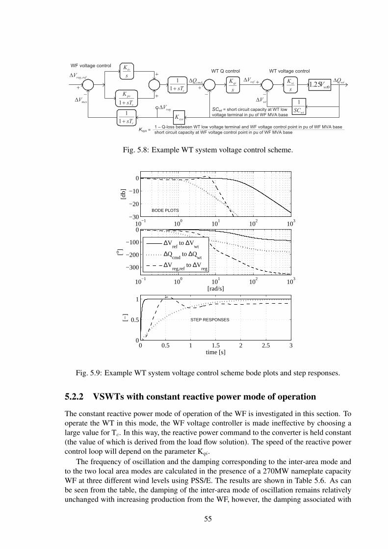
Fig. 5.8: Example WT system voltage control scheme.
10−1
100
101
102
103
−30
−20
−10
0
[db]
BODE PLOTS
10−1
100
101
102
103
−300
−200
−100
0
[o ]
[rad/s]
∆Vref
to ∆Vwt
∆Qcmd
to ∆Qwt
∆Vreg,ref
to ∆Vreg
0 0.5 1 1.5 2 2.5 30
0.5
1
[−]
time [s]
STEP RESPONSES
Fig. 5.9: Example WT system voltage control scheme bode plots and step responses.
5.2.2 VSWTs with constant reactive power mode of operation
The constant reactive power mode of operation of the WF is investigated in this section. Tooperate the WT in this mode, the WF voltage controller is made ineffective by choosing alarge value for Tc. In this way, the reactive power command to the converter is held constant(the value of which is derived from the load flow solution). The speed of the reactive powercontrol loop will depend on the parameter Kqi.
The frequency of oscillation and the damping corresponding to the inter-area mode andto the two local area modes are calculated in the presence of a 270MW nameplate capacityWF at three different wind levels using PSS/E. The results are shown in Table 5.6. As canbe seen from the table, the damping of the inter-area mode of oscillation remains relativelyunchanged with increasing production from the WF, however, the damping associated with
55

the area-2 local plant mode increases. The area-1 local mode does not change with theproduction from the WF, which is quite obvious for the investigated penetration scenario.A similar calculation is also done for a 360MW nameplate capacity WF. The results areshown in Table 5.7. A quite similar trend is also observed in this case. For the later case,the damping associated with the inter-area and the area-2 local modes are higher comparedto the previous case.
Table 5.6: Inter-area and local plant modes in the presence of a WF at various power outputfrom the WF (WF installed capacity 270MW)
inter-area (f ,ζ) area-1 (f ,ζ) area-2 (f ,ζ)
Pwt=0.25pu 0.62Hz, 0.153 1.28Hz, 0.22 1.33Hz, 0.224
Pwt=0.85pu 0.62Hz, 0.155 1.28Hz, 0.221 1.3Hz, 0.242
Pwt=1.0pu 0.62Hz, 0.155 1.28Hz, 0.221 1.29Hz, 0.246
Table 5.7: Inter-area and local plant modes in the presence of a WF at various power outputfrom the WF (WF installed capacity 360MW)
inter-area (f ,ζ) area-1 (f ,ζ) area-2 (f ,ζ)
Pwt=0.25pu 0.61Hz, 0.156 1.28Hz, 0.221 1.33Hz, 0.226
Pwt=0.85pu 0.62Hz, 0.159 1.28Hz, 0.221 1.29Hz, 0.250
Pwt=1.0pu 0.62Hz, 0.158 1.28Hz, 0.220 1.27Hz, 0.256
In the above calculations the value of the parameter Kqi is set to 0.5, as has been rec-ommended by the manufacturer, for the pf control mode of operation, especially for theEuropean WFs [38]. However, the speed of the reactive power control loop is varied bychanging this parameter, and the frequency, as well as, the damping ratio of the inter-areaand the area-2 local modes are noted. The results are shown in Table 5.8. It can be seen thatthe damping associated with the inter-area and the area-2 local modes increase with increas-ing Kqi. The frequency of the area-2 local mode decreases with increasing Kqi. However, thearea-1 local mode is not affected by this parameter variation, which is, however, not shownin the table.
Table 5.8: Inter-area and area-2 mode as affected by WT parameter Kqi (Pwt=1.0pu andinstalled capacity is 270MW)
inter-area (f ,ζ) area-2 (f ,ζ)
Kqi=0.1 0.62Hz, 0.153 1.33Hz, 0.246
Kqi=0.5 0.62Hz, 0.155 1.29Hz, 0.246
Kqi=1 0.61Hz, 0.157 1.27Hz, 0.247
Kqi=5 0.61Hz, 0.156 1.27Hz, 0.253
The WT oscillating modes under the constant reactive power mode of operation is alsoinvestigated in this subsection, which now takes the grid disturbances unlike the calculations
56
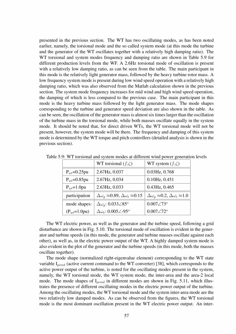
presented in the previous section. The WT has two oscillating modes, as has been notedearlier, namely, the torsional mode and the so called system mode (at this mode the turbineand the generator of the WT oscillates together with a relatively high damping ratio). TheWT torsional and system modes frequency and damping ratio are shown in Table 5.9 fordifferent production levels from the WF. A 2.6Hz torsional mode of oscillation is presentwith a relatively low damping ratio, as can be seen from the table. The main participant inthis mode is the relatively light generator mass, followed by the heavy turbine rotor mass. Alow frequency system mode is present during low wind speed operation with a relatively highdamping ratio, which was also observed from the Matlab calculation shown in the previoussection. The system mode frequency increases for mid wind and high wind speed operation,the damping of which is less compared to the previous case. The main participant in thismode is the heavy turbine mass followed by the light generator mass. The mode shapescorresponding to the turbine and generator speed deviation are also shown in the table. Ascan be seen, the oscillation of the generator mass is almost six times larger than the oscillationof the turbine mass in the torsional mode, while both masses oscillate equally in the systemmode. It should be noted that, for direct driven WTs, the WT torsional mode will not bepresent, however, the system mode will be there. The frequency and damping of this systemmode is determined by the WT torque and pitch controllers (detailed analysis is shown in theprevious section).
Table 5.9: WT torsional and system modes at different wind power generation levelsWT torsional (f ,ζ) WT system (f ,ζ)
Pwt=0.25pu 2.67Hz, 0.037 0.03Hz, 0.768
Pwt=0.85pu 2.67Hz, 0.034 0.10Hz, 0.451
Pwt=1.0pu 2.63Hz, 0.033 0.43Hz, 0.465
participation ∆ωg ≈0.89, ∆ωt ≈0.15 ∆ωg ≈0.2, ∆ωt ≈1.0
mode shapes: ∆ωg: 0.033∠85o 0.007∠73o
(Pwt=1.0pu) ∆ωt: 0.005∠-95o 0.007∠72o
The WT electric power, as well as the generator and the turbine speed, following a griddisturbance are shown in Fig. 5.10. The torsional mode of oscillation is evident in the gener-ator and turbine speeds (in this mode, the generator and turbine masses oscillate against eachother), as well as, in the electric power output of the WT. A highly damped system mode isalso evident in the plot of the generator and the turbine speeds (in this mode, both the massesoscillate together).
The mode shape (normalized right-eigenvalue element) corresponding to the WT statevariable Ipcmd (active current command to the WT converter) [38], which corresponds to theactive power output of the turbine, is noted for the oscillating modes present in the system,namely, the WT torsional mode, the WT system mode, the inter-area and the area-2 localmode. The mode shapes of Ipcmd in different modes are shown in Fig. 5.11, which illus-trates the presence of different oscillating modes in the electric power output of the turbine.Among the oscillating modes, the WT torsional mode and the system inter-area mode are thetwo relatively low damped modes. As can be observed from the figures, the WT torsionalmode is the most dominant oscillation present in the WT electric power output. An inter-
57

2 4 6 8 10
240
260
280[M
W]
Pwt
2 4 6 8 101.16
1.18
1.2
1.22
[pu]
time [s]
ωg
ωt
Fig. 5.10: WT active power, generator and turbine speed immediately after a network faultwith power factor control mode of operation (Pwt=1.0pu).
0.2
0.4
0.6
0.8
1
30
210
60
240
90
270
120
300
150
330
180 0
Activity of Ipcmd
in different modes
high wind (20m/s)
WT torsional
WT systemarea−2 local
inter−area
Fig. 5.11: Activity of Ipcmd in different oscillating modes (normalized right-eigenvectors)under constant reactive power mode of operation.
esting observation is that the activities of Ipcmd in the WT system mode and in the inter-areamode are 90o out of phase. Examining the mode shapes of the speed deviation of the con-ventional generators in the system corresponding to the WT torsional mode show that theother generators in the system do not show any activity in this mode.
58

5.2.3 VSWTs with voltage control mode of operationThis subsection investigates the WT dynamic interaction with the grid, under voltage controlmode of operation. Two different voltage control modes of operation are examined here.They are WT terminal voltage control mode and WF voltage control mode. In the WTterminal voltage control mode, the WT controls its terminal voltage to the reference voltagewhich is set from the load flow solution. In the model, this mode of operation is achieved byselecting a very high value of the parameter Tc and a very small value of Kqi. To achieve theWF voltage control mode, Tc is selected as 0.15s to represent the communication and otherassociated delays, and Kqi is selected as 0.5.
Fig. 5.12 shows the collector bus voltage and reactive power under the terminal voltagecontrol mode and the WF voltage control mode immediately after a three-phase-to-groundfault at bus 9. As can be seen from the figure, the collector bus voltage remains close tothe reference value of 1.02pu under the WT terminal bus voltage control mode, while anoscillatory behavior of 1Hz is observed under the WF voltage control mode which is due tothe WF voltage PI controller (the oscillatory behavior is also evident from the bode plot ofFig. 5.9). The eigenvalue associated with the voltage controller is calculated as -1.02±j6.24.
2 4 6 8 101
1.02
1.04
1.06
[pu]
collector bus voltage
2 4 6 8 100
20
40
60
[MV
Ar]
time [s]
collector bus reactive power
terminal voltage control modecollector voltage control mode
Fig. 5.12: WF collector bus voltage and reactive power with terminal bus voltage control andcollector bus voltage control mode following a grid disturbance.
The activity of Ipcmd in different oscillating modes under the WF voltage control modeof operation is shown in Fig. 5.13. As can be seen from the figure, the WT torsional modeis the most active and visible mode present in Ipcmd i.e. in the active power output of theturbine, followed by other oscillating modes. Comparing this figure with Fig. 5.11 reveals thedifference with the constant reactive power mode of operation. The activity of Ipcmd in powersystem modes (inter-area and area-2 local) has increased compared to the torsional mode,in the voltage control mode of operation, in addition to the new voltage control mode. Atime profile of the electric power output from the turbine will better illustrate the difference.
59

Fig. 5.14 shows the active power output from the WT following a grid disturbance underthe WF voltage control mode of operation. The difference from the constant reactive powermode of operation is visible from Fig. 5.10 and Fig. 5.14. The activity of Ipcmd in the lowfrequency oscillating mode is better damped in the WF voltage control mode of operationcompared to the reactive power control mode of operation.
0.2
0.4
0.6
0.8
1
30
210
60
240
90
270
120
300
150
330
180 0
Activity of Ipcmd
in different modes
high wind (20m/s)
WT torsional
WT system
area−2 local
inter−area
WT voltage
Fig. 5.13: Activity of Ipcmd (electric power output of the WT) in different oscillating modes(normalized right-eigenvectors corresponding to the state Ipcmd) under WF voltage controlmode of operation.
2 4 6 8 10
240
260
280
[MW
]
time [s]
Fig. 5.14: WT active power with WF bus voltage control mode following a grid disturbance.
The findings from the reactive power control mode and voltage control mode of oper-ation are summarized in Table 5.10, together with the case when the WF is modeled as aconstant MVA negative load. It can be seen that, the constant MVA negative load model-ing approach of the WF underestimates the damping associated with the inter-area mode,which is pessimistic, while, it slightly overestimates the area-2 local plant mode. The area-1mode is accurately calculated with this modeling approach. The results are summarized inTable 5.10.
60

Table 5.10: Inter-area and local plant modes in the presence of a WF together with the basecase (no WF)
Inter-area (f ,ζ) area-1 (f ,ζ) area-2 (f ,ζ)
Base case (no WF) 0.62Hz, 0.139 1.28Hz, 0.219 1.33Hz, 0.219
Q mode 0.62Hz, 0.155 1.28Hz, 0.221 1.29Hz, 0.246
vwt mode 0.62Hz, 0.153 1.28Hz, 0.221 1.29Hz, 0.245
vwf mode 0.62Hz, 0.152 1.28Hz, 0.221 1.29Hz, 0.247
(-) load 0.62Hz, 0.145 1.28Hz, 0.221 1.28Hz, 0.250
5.2.4 Grid power oscillations as affected by WT control and physicalparameters
In this subsection, the effect of changing the WT physical parameters and the control param-eters, on the power system, has been analyzed. The parameters that have been changed, oneat a time, are the WT shaft stiffness Ktg and the pitch controller proportional gain Kpp. Onlythe reactive power control mode of operation of the WF is considered here.
The value of the parameter Ktg has been changed to 0.81 from 3.16 to reduce the WT tor-sional frequency so that it coincides with the frequency of area-2 local mode of oscillation.From the normalized right-eigenvector elements associated with the speed deviations of gen-erators G3 and G4, it was found that the activity of these generators in the area-2 local modehas reduced slightly, when this change of parameter Ktg is made. However, no difference isnoted in the inter-area mode. The activity of Ipcmd is shown in Fig. 5.15. Comparing thisfigure with Fig. 5.11 shows that when the WT torsional frequency coincides with the localarea mode, the activity of Ipcmd in the system modes (inter-area and area-2 local) increases.It is also noted that the activity of Ipcmd in the area-2 local mode tries to align itself with theWT torsional mode when the torsional frequency of the WT coincides with the local areamode.
The value of the parameter Kpp is changed to 248 from 150 to increase the frequencyof the WT system mode so that it coincides with the frequency of the inter-area mode. Nonoticeable changes are noted in the mode shapes of the generators speed deviations in theinter-area mode, when this change is made. The activity of Ipcmd is shown in Fig. 5.15. Theactivity of Ipcmd in the area-2 local mode is reduced compared to the previous case. It is alsonoted that the activity of Ipcmd in the inter-area mode lead that of the WT system mode by90o.
Fig. 5.16 shows the active power response of the turbine following a disturbance with theabove mentioned changes. However, no significant difference that may harm the rest of thepower system, is noticed. In other words, the WF is decoupled from the rest of the system inthe frequency range relevant for power system stability studies.
61

0.2
0.4
0.6
0.8
1
30
210
60
240
90
270
120
300
150
330
180 0
Activity of Ipcmd
in different modes
high wind (20m/s)
WT torsionalWT system
area−2 local
inter−area
0.2
0.4
0.6
0.8
1
30
210
60
240
90
270
120
300
150
330
180 0
Activity of Ipcmd
in different modes
high wind (20m/s)
WT torsional
WT system
area−2 local
inter−area
Fig. 5.15: Activity of Ipcmd (electric power output of the WT) in different oscillating modes(normalized right-eigenvectors corresponding to the state Ipcmd), when the WT torsional fre-quency coincides with that of the area-2 local mode (left figure), and, when the frequency ofthe WT system mode coincides with that of the inter-area mode (right figure).
2 4 6 8 10
240
260
280
[MW
]
time [s]
wt torsional=>area−2 localwt system=>inter−area
Fig. 5.16: WT active power following a disturbance with the changed physical and controlparameters of the WT.
5.2.5 Discussion
In Section 5.1, it has been noted that the WT under consideration, does not show any systemmode of oscillation in low wind speed operations. Note that, in that case, the pitch controllerwas set inactive. However, in the calculations presented in Section 5.2, the pitch controlleris active even in the low wind speed region. When the pitch controller is made inactive (byincreasing the time delay associated with the pitch hydraulics in the PSS/E model), the sys-tem mode almost disappears from the eigenvalues in the low wind speed regions. Moreover,during the mid wind speed region, the system mode eigenvalue calculated in this section isdifferent from the value presented in the previous section. The reason is also due to the pitchcontroller. When the pitch controller is made inactive, the system mode eigenvalue as calcu-lated in this section agrees well with the values shown in the previous section. The resultsare summarized in Table 5.11.
62

Table 5.11: WT system mode eigenvalue during low and mid wind speed operations withand without the pitch controller
Low wind Mid wind
with pitch -0.19±j0.16 -0.33±j0.65
without pitch -1.63±j0.14 -0.16±j0.18
The frequency response from Vref of G3 to the electric power of G3 in the presence ofthe WF is shown in Fig. 5.17. It is evident from Fig. 5.17 that the generators do not interactwith the WF at the WT torsional frequency or at the WT system frequency.
Fig. 5.17: Frequency response from Vref of G3 to the electric power of G3 in the presence ofthe WF (see Fig. 5.6).
The frequency response from the initial active power reference of the WT to the electricpower output of the WT is shown in Fig. 5.18. No peak in the magnitude plot of the figure isobserved at any of the system oscillating modes, which indicates the effective decoupling ofthe WF from the rest of the system.
63

Fig. 5.18: Frequency response from the initial power reference of the WT to the WT electricpower output, when connected to the network.
The inter-area power flow in the presence of the WF together with the case when no WFis connected, following a three-phase-to-ground fault at bus 9, is shown in Fig. 5.19. Theincreased damping of the inter-area flow in the presence of the WF is noticeable from thefigure.
2 4 6 8 10
200
300
400
500
600
[MW
]
time [s]
INTER−AREA FLOW
base−casewith WF
Fig. 5.19: Inter-area power flow of the two-area system with and without the WF followinga grid disturbance.
64

Chapter 6
Frequency control support
A complete version of the analysis and results presented in this chapter can be found in
• N. R. Ullah, T. Thiringer, “Primary frequency control support from variable speedwind turbines”, IEEE Transactions on Power Systems, submitted for publication, 2008.
• N. R. Ullah, T. Thiringer, D. Karlsson, “Temporary primary frequency control supportby variable speed wind turbines – potential and applications”, IEEE Transactions onPower Systems, vol. 23, no. 2, pp. 601-612, May 2008.
For the frequency support study, where the goal is to facilitate temporary extra activepower injection into the grid based on the network frequency deviation information, the one-mass model of the drive train seems to be sufficient as the network frequency dynamic is aslower phenomena compared to the first torsional mode of the test WT (which is 16.3rad/s).In the rest of this chapter, the calculations shown are based on the one-mass representationof the WT drive train.
6.1 Quantifying the extractable rotational energy from theturbine-generator
In order to quantify the amount of energy that can be extracted from the WT, the powerthat is injected into the grid from the WT is temporarily increased by ∆Pe above its steadystate value Peo for a given wind speed. For that purpose the speed controller is disabled andthe set point for power is set independently as shown in Fig. 6.1(a) and in Fig. 6.1(b), forlow and high wind speeds, respectively. The amount of energy that can be extracted beforehitting the minimum speed limit of the turbine is calculated for different operating conditions(different wind speeds). These calculations are done in order to quantify the amount of extraactive power support a VSWT can give at a certain wind speed in addition to the steady stateelectric power at that wind speed (extra energy is coming from the stored rotational energyin the turbine-generator) and also to quantify how long such a support could be providedbefore it hits the minimum speed limit of the wind turbine. Note that, the calculations onlyrequire the equivalent inertia constant of the wind turbine-generator (HWT ), the Cp curve forthe minimum value of β (≈ 0o) and the WT rotor speed vs wind speed curve. These simplecalculations can readily give an idea about the amount of extra active power that can be madeavailable by a wind farm for bulk power system stability calculations.
65

Fig. 6.1: Simplified block diagram of the wind turbine model– (a) bypassing the controllers(low and medium wind speeds), (b) for high wind speeds taking the pitch controller intoaccount.
Notice that, when the step in the electric power is ∆Pe pu, it means that the electricaloutput from the wind turbine, Pe, is Peo+∆Pe pu (∆Pe pu higher than the steady-state valuefor this wind speed which is Peo pu). The extra ∆Pe pu power is supplied by utilizing a partof the rotational energy of the turbine-generator.
The available rotational energy is quantified for three wind speed intervals
• Low wind: The wind speed interval for which the rotor speed is less than 1.2pu.
• Medium wind: The wind speed interval for which the rotor speed is 1.2pu and thepower is less than 1.0pu.
• High wind: The wind speed interval for which the rotor speed and the power arelimited to their maximum value (1.2 and 1.0pu, respectively) and the blade pitch angleis set to higher values.
6.1.1 Low windFig. 6.2 presents the duration of a step increase in the electric power output (∆Pe) of thewind turbine for two different wind speeds (7.5m/s and 10.1m/s) before the rotor speed hitsthe 0.7pu minimum speed limit. The duration of the step increase in the output power of theWT decreases when the step size increases, as can be seen from the figure, which is obvious.At a higher wind speed, the duration of a power step is higher compared to a lower windspeed, as expected. Although the minimum speed limit of the GE 3.6MW wind turbine is0.7pu, a further reduction in the rotor speed is allowed here (down to 0.5pu). At 7.5m/s windspeed a 0.05pu extra power can be supplied for 41s when the minimum rotor speed limit is0.5pu (compared to 28s when the rotor speed limit is 0.7pu).
0.05 0.1 0.15 0.2 0.25 0.30
20
40
60
step in electric power [pu]
Tim
e to
hit
the
0.7p
um
in s
peed
lim
it [s
]
ws = 7.5m/s (P
mt= 0.3pu)
ws = 10.1m/s (P
mt= 0.75pu)
Fig. 6.2: The duration of the different step increase in the electric power output of the windturbine at different low wind speeds.
66

6.1.2 Medium windSimilar calculations are done for 10.5m/s and 11.2m/s wind speeds which correspond to0.85 and 1.0pu of wind power. At 10.5m/s wind speed, a 0.05pu extra active power supportcould be maintained for 53s before hitting the 0.7pu minimum speed limit (at 10.1m/s, thecapability was 61s). At 11.2m/s wind speed, the capability is reduced to 45s. The capabilityis reducing with increasing wind speed at the mid wind speed interval.
Despite the reduced capability of providing an extra active power support of the windturbine in the mid wind speed interval, the wind turbine under consideration can provide a0.1pu extra active power support for more than 10s quite easily before hitting the minimumspeed limit, which is twice the Hydro-Quebec requirement [16].
6.1.3 High windDuring high wind speed situations, i.e. when the speed is controlled by pitching the turbine,the active power is limited to the rated value by increasing the pitch angle with increasingwind speeds, which is done by the pitch controller. In other words, during this mode of oper-ation, an increase in the electric power output command (∆Pe) can be made available fromthe converter. Of course, this is provided that the drive train, the generator and the convertercan handle this excess power. The boost in the electric power output will shortly be com-pensated by an increase in the mechanical power input by the pitch controller (by reducingthe pitch angle) for a given wind speed (see the simplified block diagram in Fig. 6.1(b)).
Of course, these figures are dependent on the wind turbine inertia constant (HWT ) andthe shape of the Cp(λ) curve. The inertia constant and the Cp(λ) curve can vary from man-ufacturer to manufacturer. So the numbers presented here can also vary for wind turbinesfrom other manufacturers, but probably only to a smaller extent.
6.1.4 Effect of WT parameters (Cp(λ), HWT )As the Cp(λ) curve and the inertia constant HWT of a WT determine the above mentionedcapability of the WT, values of these parameters are varied from the base case values of theGE turbine and the calculations presented earlier are repeated to be able to generalize thefindings for other turbines. The following different changes in HWT and the Cp(λ) curve aremade one at a time and the results are compared with that of the GE case:
• C1: Shifting the Cp(λ) curve rightwards along the λ axis.
• C2: Reducing the maximum value of the Cp(λ) curve.
• C3: Increasing the slope of the Cp(λ) curve in the region λ<λopt.
• C4: Decreasing the slope of the Cp(λ) curve in the region λ<λopt.
• C5: Changing the value of HWT .
The reference speed (ωref ) – measured electrical power (Pef ) relationship for maximumpower tracking can also be expressed as (from [59])
Pef = (12ρAr
Sn
Cp,max(ωoR
λopt
)3)ω3ref
= Ktubω3ref (6.1)
67

where, ρ is the air density in kg/m3, Ar is the rotor swept area in m2, Cp,max is the maximumvalue of the Cp(λ) curve at β≈0o, λopt is the optimal value of λ for which the value of Cp
is maximum, Sn is the WT rating in MW, ωo is the rotor base speed in rad/s, R is the rotorradius in meter, Pef is the measured electric power in pu and ωref is the reference speed formaximum power tracking in pu. See Appendix B for the values of these parameters for theGE 3.6MW turbine. For the GE turbine, Ktub is 0.44. When λopt is shifted to 9.25 (changeC1), Ktub becomes 0.31. When the value of Cp,max is reduced by 20% from the GE case,Ktub becomes 0.35 (change C2). The effect of these changes on the corresponding Pef (ωref )curves are shown in Fig. 6.3(a). For the GE turbine, the maximum rotor speed reference1.2pu is reached at a power level around 0.75pu [58]. With change C1, the maximum rotorspeed reference is reached at a power level around 0.5pu and with C2, it reaches the maxi-mum rotor speed reference at a power level around 0.6pu, as can be seen from the figure. TheCp(λ) curve with changes C3 and C4 are shown in Fig. 6.3(b) together with the GE case.
0.8 1 1.2
0.2
0.4
0.6
0.8
(a)
ωref
P ef
GEC2C1
5 6 7 80.3
0.4
0.5(b)
λ
Cp
GEC3C4
Fig. 6.3: (a) Optimal rotor speed - power curve for maximum power tracking with changesC1 and C2 together with the GE case, (b) Cp(λ) curve in the region λ<λopt with changes C3and C4 together with the GE case.
Fig. 6.4 shows the temporary extra active power support capability of the turbine withchanges C1 and C2 together with the GE case at different low and medium wind speeds.When the Cp(λ) curve is shifted rightwards i.e. λopt is changed to 9.25 (change C1), theabove mentioned capability increases in low wind speeds compared to the GE case and themaximum capability occurs at a wind speed of 8.8m/s. On the other hand, the same capabilitydecreases in the medium wind speeds compared to the GE case (see Fig. 6.4). However, nosignificant changes in the above mentioned capability are noticed when the maximum valueof the Cp(λ) curve is reduced by 20% from the GE value (change C2), as can be seen fromthe figure.
Fig. 6.5 shows the above mentioned capability with changes C3 and C4. With increasingslope of the Cp(λ) curve in the region λ<λopt, the capability of providing a certain excesspower at a certain wind speed decreases, as can be seen in Fig. 6.5. Also note that, the abovementioned capability decreases almost linearly when HWT is reduced (see Fig. 6.5).
With the changes in HWT and the Cp(λ) curve that are made, it is found that the WTunder consideration can provide 0.1pu of extra active power support for more than 10s,except for some lower values of the inertia constant (HWT <3.6s).
68

7 8 9 10 11
20
40
60
min
spe
ed li
mit power step
= 0.05pu
7 8 9 10 11
10
20
30
40
wind speed [m/s] T
ime
to h
it th
e 0.
7pu
power step
= 0.1pu
Fig. 6.4: The capability of the WT to provide 0.05 and 0.1pu of extra active power before hit-ting the 0.7pu minimum speed limit of the turbine at low and mid wind speeds with changesC1 and C2 together with the GE case. Legends are the same as in Fig. 6.3(a).
3 4 520
40
60
0.7p
u sp
eed
limit
[s]
w
s = 7.5m/s
X
power step= 0.05pu
3 4 520
40
60
ws = 10.1m/s
X
3 4 520
40
60
ws = 10.6m/s
X
3 4 510
20
30
40
Tim
e to
hit
the
X
power step= 0.1pu
3 4 510
20
30
40
HWT
[s]
X
3 4 510
20
30
40X
Fig. 6.5: The capability of the WT to provide 0.05 and 0.1pu of extra active power beforehitting the 0.7pu minimum speed limit of the turbine with changes C3 and C4 together withthe GE case against HWT . ’X’ represents the GE case HWT =5.19s. Legends are the same asin Fig. 6.3(b).
6.2 Possible signal injection points for the temporaryprimary frequency control (TPFC) function
An automatic method to facilitate the TPFC function from an example WT system is pro-posed and evaluated in this chapter.
6.2.1 Requirements on the TPFC
The main functional requirements from the TPFC are:
• An increase in the electric power output should be maintained beyond the temporaryminimum frequency (TMF) point.
69

• Subsequent reduced power generation from the grid to accelerate the WT rotationalspeed to the optimal operating point (during low wind speed operations) should becarried out over a longer period of time to minimize any adverse effect on the grid.
• The value of the subsequent absorbed power should be lower than the previously in-jected power.
6.2.2 Low wind speed operationsThe disturbance rejection capability of the test WT system is analyzed in this subsection.The transfer function from the disturbing signal (either as a speed reference disturbance, asshown in Fig. 6.6 as ‘A’, or an electric power command disturbance, as shown in Fig. 6.6as ‘B’) to the delivered electric power of the WT has been determined and Fig. 6.7 showsthe bode plot and the time series of the delivered electric power when a step disturbance isapplied. It can be seen from this figure that an electric power command disturbance diesout quickly compared to a speed reference disturbance. Two non-oscillatory modes (withassociate time constants) and the corresponding residues, normalized to the slower mode(when a step disturbance is applied), are shown in Table 6.1. The residue, when a speedreference is applied, is labeled as RA, and the other one is labeled as RB. As can be seen,the faster decaying mode has a higher residue compared to the slower mode. However, whenan electric power command disturbance is applied, the residue corresponding to the slowermode has a negative value which explains the negative undershoot in Fig. 6.7(b). It can alsobe seen that the dynamics of the delivered electric power into the grid upon experiencinga power command reference disturbance is mainly determined by the faster mode. On theother hand, when a speed reference disturbance is applied, the dynamics of the deliveredelectric power are dependent on both the modes.
Fig. 6.6: Block diagram of the example WT model, adopted from [58]. Values of differentparameters are given in Appendix B.
70

10−2
100
102
−40
−20
0
(a) ω*−Pe
Gai
n [d
b]
10−2
100
102
−40
−20
0
(b) P*−Pe
10−2
100
102
−50
0
50
Ang
le [o ]
[rad/s]10
−210
010
2
−500
50100150
[rad/s]
0 5 10 150
2
4
time [s]
P e [pu]
Pwt=0.25puPwt=0.70puPwt=0.90pu
0 5 10 15
0
0.5
1
time [s]
Fig. 6.7: Disturbance rejection capability of the test WT system. See Fig. 6.6 for the distur-bance injection points.
Table 6.1: Time constant (TC) and residue normalized to the slower mode (R) of two domi-nant non-oscillatory modes at Pwt=0.25pu
Mode TC RA RB
Mode–1: -0.0721 13.2s 1.0 -1.0
Mode–2: -0.852 1.2s 5.2 11.4
Instead of a step disturbance (either as a speed reference or a power command reference),a disturbance similar to the network frequency fall and recovery, is applied and the responseof the test WT is observed. The time profile is shown in Fig. 6.8. The amplification ofthe network frequency deviation signal is adjusted so that an equal peak power of 0.05puis obtained in both cases. As can be seen from these simulations, the subsequent powerabsorption from the grid is larger when the disturbance is a power command disturbancecompared to the speed reference disturbance. The excess power output from the turbine isalso maintained for a longer time when a speed reference disturbance is applied, comparedto the power command disturbance. In the figure, the change in WT speed is also shown.
So, the speed reference disturbance rejection capability of the test WT system gives afavorable electric power output profile that suits the requirement of the frequency controller.
71

0 10 20 30 40−0.05
0
0.05∆
P e [pu]
network frequencydisturbance equivalent
0 10 20 30 40−0.05
0
0.05
∆ ω
wt [p
u]
time [s]
ωwt
disturbance
Pe disturbance
Fig. 6.8: Response from the turbine generator system when a disturbance similar to a net-work frequency disturbance is applied either as a speed reference disturbance or as a powerreference disturbance. For the purpose of comparison amplification of the disturbance signalhas been adjusted so that an equal peak power of 0.05pu is obtained in both cases. The initialcondition is Pwt = 0.25pu.
6.2.3 Disturbance rejection capability as affected by WT parametervariation
The disturbance rejection capability of the test WT system (shown earlier) as affected by thevariation of different WT parameters, such as, control parameters variation (WT speed con-troller damping (ζt) and bandwidth (ωnt)), and physical parameter variation (WT equivalentinertia constant HWT ), are analyzed here.
The parameters of the speed controller (ζt, ωnt) are varied from the GE values to identifyhow the disturbance rejection capability of a WT system with different controller settingswill vary and affect the TPFC performance. The calculation of ζ and ωn for the test WT isshown in Appendix B. The example WT system speed controller parameters are identifiedas ζt=0.6 and, ωnt=0.24rad/s. The locus of two non-oscillatory modes together with residuesRA and RB are shown in Fig. 6.9 with varying ωnt and ζt, and in Fig. 6.10 with varyingHWT . Note that the filter time constant Tf is kept as Kit/Kpt to nullify the effect of the poleat - 1
Tf.
A time domain simulation will better illustrate the effect of changing the WT parameterson the electric power output of the WT. Such a simulation is shown in Fig. 6.11 with sixdifferent parameter settings. The settings are as follows:
• S-1: ζt=0.6, ωnt=0.24rad/s, HWT =5.19s (example WT setting).
• S-2: ζt=0.5, ωnt=0.50rad/s.
• S-3: ζt=0.7, ωnt=0.20rad/s.
72

• S-4: ζt=0.7, ωnt=0.50rad/s.
• S-5: ζt=0.5, ωnt=0.20rad/s.
• S-6: Same as S-1 except for HWT =3s.
0.1 0.2 0.3 0.4 0.5
10
12
14
16
TC
[s]
Mode−1
X
ζt =0.7
ζt =0.6
ζt =0.5
ζt =0.2
0.1 0.2 0.3 0.4 0.50.5
1
1.5
2
2.5
Residue RA
[−]
ζt =0.2
ζt =0.5
ζt =0.7
X
0.1 0.2 0.3 0.4 0.5
−4
−3
−2
−1
0
Residue RB
ζt =0.7
ζt =0.2
X
0.1 0.2 0.3 0.4 0.50
1
2
3
[s]
Mode−2
ζt =0.2
ζt =0.7
X
0.1 0.2 0.3 0.4 0.50
10
20
30
ωnt
[rad/s]
[−]
ζt =0.7
ζt =0.2X
0.1 0.2 0.3 0.4 0.510
15
20
25ζ
t =0.7
ζt =0.2
X
Fig. 6.9: Loci of time constants and residues of two dominant non-oscillatory modes of thetest WT as affected by the control parameter (ζt, ωnt) variation. ’×’ denotes the base case.Residues are normalized to the slower mode of the base case. Initial condition is Pwt =0.25pu. Above diagrams assume Tf=Kpt
Kit= 2ζt
ωnt.
3 4 5
2
4
6
8
10
12
14TC
[s]
Mode−1
Mode−2
3 4 5
1
2
3
4
5
Residue RA
HWT
[s]
Mode−1
Mode−2
3 4 5
0
5
10
Residue RB
Fig. 6.10: Ratio of time constants and residues of two dominant non-oscillatory modes ofthe test WT as affected by the WT inertia constant HWT variation. Residues are normalizedto the slower mode of the base case. Initial condition is Pwt = 0.25pu. Above calculationsassume Tf=Kpt
Kit= 2ζt
ωnt. ζt and ωnt are fixed to the base case values.
73

As can be seen from Fig. 6.11, no significant differences are observed, however, the speeddisturbance rejection tends to be slower when the speed controller bandwidth is increased,as well as, the damping is reduced.
0 5 10 15 20 25
0
0.5
1
Time [s]
∆ P e [−
]
S−1S−2S−3S−4S−5S−6
Fig. 6.11: Response from the turbine generator system when a disturbance similar to a net-work frequency disturbance is applied as a speed reference disturbance for six different pa-rameter settings. Initial condition is Pwt = 0.25pu.
6.2.4 High wind speed operation
In high wind speed operation, the disturbance rejection capability of the WT does not needto be considered. An additional electric power command can be added as shown in Fig. 6.12.The WT speed will momentarily increase but will be brought back to the set value of 1.2 puby the pitch controller. However, the mechanical power will also increase to offset the in-creased active power injection into the grid, so that the rotational speed is maintained at therated value. Important to note is that the turbine mechanical design and the machine sideconverter power rating need to be properly dimensioned for this purpose.
Fig. 6.12: The example WT block diagram showing the additional signal injection pointduring high wind speed operation.
6.2.5 Gain adjustment
To facilitate the temporary extra active power support from a VSWT, a proportional con-troller is proposed whose gain is adjusted to provide a certain excess active power for thenetwork dimensional disturbance. It has been noticed that the overall gain of the test WT
74

system is dependent on the operating point or on the prevailing wind condition. So, a vari-able gain proportional controller is considered here, see Fig. 6.13 for the structure of theproposed controller, where Pe0 is the initial electric power output from the WT depending onthe prevailing wind condition. When the network frequency deviation (∆ωr) exceeds a cer-tain dead-band zone, the TPFC is activated. The WT prevailing power output and the pitchangle information is used to identify the WT operating state when the network frequency dis-turbance occurs. Based on the WT operating state, an appropriate gain is calculated. Whena non-zero or non-optimal pitch angle is detected, this means that the WT is operating in thehigh wind speed region. When such a state is detected, the TPFC generates a power distur-bance signal to be fed into the WT system, as shown in Fig. 6.13. For other operating states,a speed reference disturbance signal is generated.
Fig. 6.13: Proposed TPFC structure.
For a certain dimensional disturbance, the necessary gain profiles to deliver maximum5% and 10% extra active power, are shown in Fig. 6.14. For a certain dimensional generationdisconnection scenario, the network frequency will drop and reach its minimum after a fewseconds before returning to the new steady-state value in another few seconds. Usually,the rate of frequency recovery is slower than the rate of frequency decay. For the TPFCgain setting purpose, a hypothetical ‘frequency fall and recovery function’ equivalent to theactual network frequency profile (see Fig. 6.8), is used to determine the TPFC gain profilefor different TPFC strengths. The TPFC gain profiles shown in Fig. 6.14 are determined inthis way.
6 8 10 12
5
10
15
20
25(a)
wind speed [m/s]
Gtp
fc [−
]
for 10% max. ∆Pe
for 5% max. ∆Pe
0.2 0.4 0.6 0.8 1
5
10
15
20
25(b)
Pe [pu]
for 10% max. ∆Pe
for 5% max. ∆Pe
Fig. 6.14: Gain profile of the TPFC with different strengths (5% and 10%).
75

6.3 Impact on the existing power system
In this section, the impact of the WF TPFC on the operation of the speed governing systemof the existing power system is analyzed.
6.3.1 Cigre Nordic 32-bus power system for load frequency control study
To investigate the impact of the TPFC on the existing frequency control set-up of the powersystem, the Cigre 32-bus test system is adopted as a base case. Details regarding the testsystem can be found in [61]. The system generation portfolio is as follows:
• External hydro – 5000MVA installed capacity, H=3s.
• Northern hydro – 5950MVA installed capacity, H=3s.
• Thermal generation – 6000MVA installed capacity, H=6s.
• Synchronous condenser – 300MVA installed capacity, H=2s.
The totally installed capacity is thus 17250MVA. The load in the system is 10940MW witha load damping factor of 0.75% (D=0.75). The totally installed capacity of 17250MVA istaken as the system MVA base. On this base, the system inertia Heq becomes 4.03s and thesystem load damping factor D becomes 0.48.
The automatic system frequency control task is mainly carried out by hydro generators inthe system. The thermal generators are not participating in the frequency control. The hydrogovernor model used in the original test system is the PSS/E library model HYGOV [68].Two different droop settings are used for the external and the northern hydro generators.External hydro generators permanent and temporary droop settings are 0.08 and 1.6, respec-tively. On the other hand, the corresponding settings for the northern generators are 0.04and 0.8, respectively. On the system MVA base, the equivalent permanent droop RP,eq of thesystem is 0.0817 and the equivalent temporary droop RT is 1.63. Water starting time TW ,reset time TR and servo time constant TG are 1.0s, 5s and 0.25s, respectively, for all hydrogenerators. The single mass representation of the test power system for the load frequencycontrol study is shown in Fig. 6.15, where Lp is the wind power penetration in per-unit ofthe totally installed generation capacity.
Fig. 6.15: Single mass representation of the Cigre Nordic 32-bus test system for the loadfrequency control study including the TPFC.
76

6.3.2 Wind power integration scenarioThe coming wind power integration scenarios into the existing power systems may varyconsiderably. For instance, the incoming wind power may replace existing conventionalgenerators which were contributing/not contributing to the primary frequency control, orthe incoming wind power may be utilized for the coming load growth. The impact of thewind power integration on the system frequency control function will also depend on theintegration scenarios.
It is assumed that the system load remains the same (i.e. 10940MW) and the incomingwind power replaces thermal generation units which means that the phased out generatorswere not contributing to the primary frequency control function. So, the system frequencycontrol strength remains the same even after the wind power is integrated into the system.The only difference it makes is that the system inertia will be less compared to the basecase scenario which will influence the TMF of the system after a generation deficit situation,unless control parameters are re-tuned. The motivation for this assumption is that in Swedenseveral large WFs are being planned [8, 9] and in the future some nuclear power plants maybe phased out which are not currently contributing to the primary frequency control of thesystem (two units of the nuclear power plant Barseback, situated near Malmo, have alreadybeen phased-out [66]).
1500MW of wind power has been assumed to be integrated into the system. With thisintegration, the system equivalent inertia constant Heq becomes 3.51s on the same systemMVA base. The permanent droop of the system is not affected by the wind power integrationas the phased out generators were not contributing to the primary frequency control.
6.3.3 Incoming wind power with TPFC option and its impact on theexisting speed governing system
The gain profile of the TPFC is set such that an extra active power of maximum 5% of theWF installed capacity can be delivered (TPFC strength is 5%), when the network frequencyis outside its normal range of 50±0.1Hz and reaches as low as 49.5Hz. See Fig. 6.14 for thegain profile to provide a maximum 5% extra active power.
The open-loop frequency response characteristic of the speed governing system of theCigre test system is shown in Fig. 6.16(a) together with the case when the integrated WFs areequipped with TPFC function. The phase and gain margins [69] of the open-loop frequencyresponse characteristic of the speed-governing system of the Cigre test grid are calculated as49o (at 0.13rad/s) and 20.1db (at 0.95rad/s), respectively, which are in accordance with theANSI/IEEE recommendation [70]. Including the WF with TPFC, the phase and gain mar-gins become 56.1o (at 0.1rad/s) and 21.1db (at 1.14rad/s), respectively. The gain and phasemargins of the Cigre system have improved in the presence of the WF with the TPFC featurewhich can be seen as an improvement of the stability of the speed governing system. How-ever, note that the response of the speed governing system becomes slower in the presence ofTPFC which can be seen from the crossover frequencies (the value of frequency for whichthe magnitude is unity or 0db) [24].
Fig. 6.16(b) shows the closed-loop frequency response characteristics of the base caseCigre system and the augmented system with WFs featuring TPFC from ∆PL to ∆ωr. Fromthe gain plot, it can be seen that in the time domain the TMF will be lower in the presence ofWFs with TPFC when a sudden loss of generation occurs in the system.
77

10−2
10−1
100
101
−40
−20
0
20
(a) open−loopG
ain
[db]
10−2
10−1
100
101
−40
−30
−20
−10
0
(b) ∆PL − ∆ω
r
base casewith TPFC
10−2
10−1
100
101
100
150
200
250
300
Ang
le [o ]
[rad/s]10
−210
−110
010
1
100
150
200
250
[rad/s]
Fig. 6.16: (a) Open-loop frequency response characteristic of the speed control system ofthe Cigre Nordic 32-bus test system with and without the TPFC, (b) closed-loop frequencyresponse characteristic of the above mentioned system with and without the TPFC from ∆PL
to ∆ωr.
The network frequency profile after a generation disconnection scenario is shown inFig. 6.17 with a WF with and without TPFC together with the base case. As expected,the network TMF is reduced with the WF TPFC, whereas the frequency recovery becomesslower compared to the base case. For the purpose of comparison, the frequency profileincluding WF without TPFC is also shown in the figure. The network frequency drops fur-ther down transiently as the system inertia is reduced compared to the base case as someconventional generators were phased out.
0 20 40 60
−0.4
−0.2
0
Time [s]
∆ωr [H
z]
base caseno TPFCwith TPFC
Fig. 6.17: The network frequency profile after a generation disconnection with a WF withand without TPFC together with the base case. The TPFC strength is 5%.
78

The WF electric and mechanical power together with the rotational speed in the presenceof TPFC are shown in Fig. 6.18. Note that, the subsequent power absorption from the gridto accelerate the rotational speed of the WT to it’s optimal value is done over a longer periodof time. This will minimize any adverse effect on the network frequency recovery. Also,note that the WT mechanical power is reduced during this temporary active power supportprocess, although the wind speed remains the same.
0 20 40 60−0.05
0
0.05
Time [s]
[−]
∆Pe
∆Pmt
∆ωwt
Fig. 6.18: WF response in the presence of the TPFC feature.
6.3.4 Governing system parameter resetting in the presence of a WFwith the TPFC option
As has been noticed before, the network frequency recovery process has been slowed downin the presence of the TPFC function from WFs, although the TMF is improved. As the mainfrequency regulation function is carried out by the conventional generators, their governorsettings need to be adjusted.
Both RT and TR are modified simultaneously to restore the original system stabilitycharacteristics. The gain margin and the crossover frequency of the open-loop frequencyresponse characteristic of the governing system are 20.1db and 0.13rad/s, respectively, forthe Cigre test case. These values are taken as the benchmark stability characteristics. Theintersection point of the 20.1db gain margin locus and the 0.13rad/s crossover frequencylocus correspond to the Cigre system governor setting. In the presence of a WF without theTPFC option, the necessary setting to maintain the benchmark stability properties changes, asshown in Fig. 6.19. In the presence of WFs with the TPFC option, a 20.1db gain margin locuscan be observed in Fig. 6.19 when both RT and TR are varied. The benchmark 0.13rad/scrossover frequency locus is also drawn in the same figure. The intersection point is the newsetting of the governor parameters where both the gain margin and the crossover frequencyare restored to base case values. The locus of the intersection point is also shown in thefigure with increasing TPFC strength. It can be seen that both RT and TR need to be reducedwith increasing TPFC strength to maintain the benchmark stability characteristics.
For the studied wind power penetration scenario and the TPFC strength, the reset timeand the temporary droop of the existing governing system are reduced to 3.64s and 1.54,respectively, from their initial values of 5s and 1.63, respectively, to restore the benchmark
79

5 10 15
0.8
1
1.2
1.4
1.6
1.8
2
TR [s]
RT [−
]
20.1 db gain margin locus
0.13 rad/sec crossover freq. locus
XOO
OX− Cigre system setting
O− Modified settings with TPFC
increaseing∆ P
e
∆ Pe=0%
∆ Pe=7%
2%
5%
Cigre casewind without TPFCwind with TPFC
Fig. 6.19: Loci of constant gain margin and crossover frequency.
0 20 40 60
−0.4
−0.2
0
Time [s]
∆ωr [H
z]
base casewith TPFCmodified settings
Fig. 6.20: Network frequency profile with the modified settings of RT and TR, as shown inFig. 6.19.
stability characteristics. The result is a faster frequency control capability, without degradingthe stability of the overall governing system. The frequency profile of the network with thisnew setting of RT and TR is shown in Fig. 6.20 together with the base case. The TMF isimproved by 0.1Hz and the frequency recovery becomes faster in the presence of WFs withthe TPFC option, when the suggested changes are made in the existing governing system.
80

Chapter 7
Reactive power ancillary serviceprovision – technical and economic issues
A complete version of the analysis and results presented in this chapter can be found in
• N. R. Ullah, K. Bhattacharya, T. Thiringer, “Wind farms as reactive power ancillaryservice providers – technical and economic issues”, IEEE Transactions on EnergyConversion, accepted for publication, paper no. tec-00137.2008.
7.1 Reactive power capability of WFs under different gridcodes
7.1.1 Investigated WF layoutA VSWT with a full scale power electronic converter is shown in Fig. 7.1, where Ic isthe converter output current. The typical layout of a WF is shown in Fig. 7.2 wherein,Vg, P and Q represent the voltage at the grid connection point, the WF active and reactivepower production at the grid connection point, respectively. Vc represents the convertervoltage, which depends on the dc-link voltage of the converter (Vdc), on the modulationtechnique used and on the amplitude modulation index [55]. For a given hardware setup, Vc
has a certain maximum value. X1 represents the total reactance of the wind turbine’s step-up transformers and the grid filters (10%), X2 represents the reactance of the transformertransforming the wind turbine’s medium voltage to 400kV (20%).
Fig. 7.1: A VSWT with a full scale back-to-back power electronic converter comprising amachine-side (MSC) and a grid-side converter (GSC).
81

Fig. 7.2: A typical wind park layout considered in the work.
7.1.2 Limiting factorsThe grid-side converter (GSC) has a certain maximum current carrying capacity, which willimpose a limit on the P and Q-capability of the turbine. In the PQ plane, it will be a circlesimilar to that of the armature current limit of a synchronous generator, as shown in Fig. 7.3.The relationship between the active and reactive power at the converter current limit is
P 2 + Q2 = (VgIc)2 (7.1)
where, Ic is the converter current.
Fig. 7.3: Capability curve of a VSWT with full scale power electronic converter.
The converter voltage Vc will impose another limit on the P and Q capability of the windturbine, which is similar to that of the field current limit of a synchronous generator. Basedon these analogies of the capability curve of a wind turbine with a full power converter (see
82

Fig. 7.1) with that of a conventional synchronous generator [24], the relationship between Pand Q at the converter voltage limit is given by,
P 2 + (Q +V 2
g
X)2 = (
VcVg
X)2, (7.2)
where, X is the total equivalent reactance from the wind turbine low voltage terminal to thegrid connection point (see Fig. 7.2). Equation (7.2) represents a circle in the PQ plane withcenter (c) and radius (r) as given in (7.3)
c = (0,−V 2g
X), r =
VcVg
X. (7.3)
7.1.3 Design valuesGrid codes of utilities often require a WF to be able to operate continuously at the ratedpower at a certain pf within a certain band of voltages and frequencies at the grid connectionpoint, see [18, 19] for examples. Let us define the upper and lower values of voltage andfrequency as Vg,max=1.05, Vg,min=0.9, fmax=1.01 and fmin=0.98, respectively (all in pu),and the rated pf as cosθR, where θR is the rated power factor angle of the WF. These limitvalues can be used to calculate the design value or the maximum value of the convertervoltage (Vc,max), which determines the maximum dc-link voltage (Vdc,max) of the converter,as well as the maximum current rating (Ic,max) of the converter. Note that, it is assumed thatthe grid reactive power requirement is met by the built-in converters of the wind turbines andaccordingly, the design values Vc,max, Ic,max and Vdc,max are determined. See the appendedpaper Paper-IV for the derivation of the design values.
The maximum reactive power injection capability from the WF is calculated as,
Q = minQc, Qv (7.4)
where, Qc and Qv are the converter current rating and voltage rating limited reactive powerproduction from the WF, respectively, at a certain level of active power production. Qc andQv are given by
Qc =√
(VgIc,max)2 − P 2, (7.5)
Qv =
√(Vc,maxVg
X)2 − P 2 − V 2
g
X. (7.6)
The maximum converter current and voltage ratings as well as the power rating for dif-ferent design pf cases are summarized in Table 7.1. In the table, the corresponding maximumdc-link voltage is also given.
7.1.4 WF reactive power capability considering wind variationsThe power generated from a WF varies considerably over the daily cycle. The reported windplant integration study [71] by Xcel Energy North considered wind forecast errors in therange of ±10 to ±50%. It is reported in [48] that a reasonable day ahead hourly wind powerforecast, using the state-of-the-art forecasting tools, will have a mean absolute error of 10–15% of the rated capacity of the WF. The frequency distribution of the day-ahead wind power
83

Table 7.1: Ic,max, Vc,max, Pc,max and Vdc,max for different design casespf = 1.0 pf = 0.95 pf = 0.9
Ic,max [pu] 1.11 1.17 1.24
Vc,max [pu] 1.09 1.17 1.21
Pc,max [pu] 1.21 1.37 1.50Vdc,max [pu] 1.54 1.66 1.71
forecasting error in Germany reveals a maximum ±25% error [49]. Such a high degree ofvariability of the actual hourly wind power from the forecasted value reduces the availablereactive power capability of the WF from the actual capability, derived in Subsection 7.1.3.This reduced capability should be reported to the ISO as the available hourly reactive powercapability of the WF.
The actual reactive power capability of the WF (Qac,k), when the forecasted wind poweris P ∗
k , at kth hour of operation is obtained from (7.4) as,
Qac,k = minQc,ac,k, Qv,ac,k (7.7)
where,
Qc,ac,k =√
(VgIc,max)2 − P ∗2k , (7.8)
Qv,ac,k =
√(Vc,maxVg
X)2 − P ∗2
k − V 2g
X. (7.9)
Qc,ac,k and Qv,ac,k are the actual converter current rating and voltage rating limited re-active power capability, respectively, at the kth hour of operation. However, due to the highdegree of variability of actual wind power in both directions from the forecasted value, deliv-ery of Qac,k can not be guaranteed by the WF over the entire hour of operation. The WF maylose significant amount of revenue from its energy sold if Qac,k is reported to the ISO as theavailable amount of reactive power (Qav,k) at the kth hour of operation based on forecastedwind power P ∗
k . In that case, the WF has to limit its active power production to P ∗k .
The wind variation has to be taken into account while determining the available/guaranteedreactive power. Based on available meteorological data, the maximum hourly variation ofwind power generated from the forecasted value (∆Pmax, in pu of installed capacity of theWF) can be determined or be agreed upon which can be updated once every year or month.∆Pmax will depend on the specific site [48]. The available reactive power at the kth hour(Qav,k) can now be determined from (7.10) as follows:
Qav,k = minQc,av,k, Qv,av,k (7.10)
where,Qc,av,k =
√(VgIc,max)2 − P ∗2
max,k, (7.11)
Qv,av,k =
√(Vc,maxVg
X)2 − P ∗2
max,k −V 2
g
X, (7.12)
P ∗max,k = P ∗
k + ∆Pmax, (7.13)
84

∆Pmax ≤ P ∗max,k ≤ 1. (7.14)
The available Q-capability of the WF and its comparison to the actual Q-capability isshown in Fig. 7.4 for design pf=0.95.
0 0.2 0.4 0.6 0.8 1
0.4
0.5
0.6
0.7
P*k [pu]
Qac
,k [
pu]
actual capability
availablecapability
X
∆ Pmax
=0.2
∆ Pmax
=0.5
Vg = 0.95
Fig. 7.4: Available Q-capability considering wind variations compared to actual Q-capabilityat Vg=0.95pu, design pf=0.95 (considering ∆Pmax=0.2 and 0.5pu). Only the capacitive ca-pability is shown.
7.2 Cost components of reactive power from a WF
7.2.1 Fixed cost componentIn [72], the breakdown of the levelized production cost of a baseline offshore WF, equippedwith DFIG type wind turbines, is reported. Six main cost components are identified in [72]as the first level components, which are:
• hardware (including onshore transportation) (51%),
• yearly operation and maintenance (O&M) (29%),
• assembly, transport and installation (10%),
• retrofit and overhaul (7%),
• decommissioning (2%), and
• WF design (1%).
To extract the investment cost components, only the following components need to beconsidered:
• hardware (including onshore transportation) (82%),
85

• assembly, transport and installation (16%), and
• WF design (2%).
The breakdown of the hardware cost at the second level consists of mainly the WECS costwhich is around 80% of the hardware cost component, and the electric collection and trans-mission system cost which is around 12% of the hardware cost [72]. The breakdown of theWECS cost at the third level consists of mainly three components [72], which are
• support structure (44%),
• nacelle (32%), and
• rotor (24%).
The electric conversion system cost, i.e. the power electronic converter cost, and the com-puter and sensors cost are around 5% and 26% of the nacelle cost, respectively [73]. Notethat, the reported cost model analysis in [72,73] is done based on a DFIG type of WT, wherethe converter handles only around 30% of the rated power. However, in the case of a full-power converter system, the converter handles the full rated power of the WT. So, we canexpect that, in such cases, the converter cost can be around 15% of the nacelle cost, assumingthat the converter cost varies linearly with the power rating of the converter [74].
From the above mentioned cost figures, we can conclude that the back-to-back full-powerconverter (carrying only the rated active power of the turbine) cost is around 3% of the totalinvestment cost, and the converter control system cost is embedded as a small part of thecomputer and sensors cost, as can be expected. The GSC cost is half of the total back-to-back converter cost i.e. the GSC cost is 1.5% of the total investment cost of the WF.
If the GSCs are designed to comply with the reactive power requirements of the WFat the grid connection point, then the cost will increase. Note that, the additional reactivepower support is provided by the grid-side VSC. The cost of the GSC, in percentage of thetotal investment cost of the WF, to comply with 1.0, 0.95 and 0.9 pf requirement at the gridconnection point are 1.8%, 2% and 2.25%, respectively, calculated from the required powerrating of the converter (see Table 7.1).
7.2.2 Cost of lossesThe additional active power losses incurred by the WF because of an increased reactivepower demand from the ISO need to be calculated for financial compensation purpose, ifit accounts for a significant value. In cases where the reactive power demand is met bythe grid-side VSC of the built-in back-to-back converter of the WTs, as considered in thiswork, the additional active power losses due to increased reactive power supply from theWF mainly occur in the GSC switches and in the resistances of transformers/cables. Seeappended Paper-IV for the derivation of losses in the converter switches.
The losses of a 1MW power module are calculated as a percentage of the rated power ofthe converter for the following scenarios, assuming unity pf design case and Vg=1.0 pu:
1. scenario-1: rated operation, unity pf. Losses = 1.15%,
2. scenario-2: 50% of rated operation, unity pf. Losses = 0.52%,
86

3. scenario-3: 50% of rated operation, 0.9 pf. Losses = 0.58%.
See [75] for the data sheet of the power module. The losses in the power module increases by12% when 25% reactive power is supplied at 50% rated operation in scenario-3 as comparedto scenario-2. The increase in active power losses is 0.06% of the rated value. On theother hand, when the reactive power demand is met by reducing the active power production(reducing the active power production to 50% of the rated value from the 100% operation toprovide 25% reactive power), the power losses decreases by 0.57% of the rated value.
As the power module will be used in a parallel configuration in a multi-MW WT, thepercentage or the pu losses in the GSC, on the WT base quantities, will be the same. Thisvalue will increase or decrease depending on the amount of reactive power supply from themodule, as can be expected. Although not significant, a certain amount of increased activepower losses can be incurred by the WF or can be reduced by the WF, while fulfilling theISO’s request to increase the reactive power production from the mandatory value (grid coderequirement), with or without reducing the present active power production. The cost ofthese power losses can be considered by the ISO while formulating mechanisms for reactivepower procurement from WFs.
7.2.3 Opportunity cost componentIf the WF has to decrease its active power generation and hence forgo market opportunityin order to fulfill an ISO request for additional reactive power, then the WF should receivea payment to cover its lost opportunity cost (LOC). Conventional generators receive suchpayment in some electricity markets [76].
Because of the high degree of variability of the wind speed during an hour, it is difficultfor the WF to guarantee the provision of a certain amount of reactive power to the ISO basedon the forecasted power. The maximum hourly variation of wind power from historical dataneeds to be considered, and the method of calculating the available amount of reactive powerconsidering the hourly wind variation has been introduced in Subsection 7.1.4.
Furthermore, it would be difficult for the ISO to determine the LOC for a WF, since theISO will not have information on whether the wind speed was naturally low (so that theWF could provide the enhanced reactive power supply) or it acted on the ISO´s request forincreased reactive power supply. In this subsection, a procedure to calculate the LOC for aWF is proposed.
When the forecasted wind power is P ∗k at the kth hour of operation, the actual reactive
power capability is Qac,k (see Fig. 7.5). However, this amount of reactive power cannot beuniformly guaranteed by the WF during the entire kth hour of operation. Due to the highdegree of variability of wind, the actual production of the WF can exceed the forecastedvalue during the hour. Taking such variations into account, a value ∆Pmax can be estimated,which can, for instance, be based on previous meteorological data. The kth hour wind powerforecast P ∗
k , can now be immediately converted to a forecasted maximum wind power P ∗max,k
given byP ∗
max,k = minPR, P ∗k + ∆Pmax, (7.15)
where, PR is the rated active power of the WF. The available reactive power from the WF atthe kth hour of operation is Qav,k, considering the hourly wind variation, as shown in Fig. 7.5.Now, if the reactive power demand from the ISO is Qr,k, which is in excess of Qav,k, then itwill impose a highest limit on the active power production (Plim,k). In other words, to fulfill
87

the ISO reactive power demand of Qr,k, which is ∆Qk in excess of the available reactivepower capability, the WF may lose ∆Pk active power production, where
∆Pk = P ∗max,k − Plim,k. (7.16)
∆Pk is the amount of the lost active power production that the WF should be compensatedfor, in the form of LOC.
Fig. 7.5: Concept of LOC component calculation for a WF.
During the operational planning phase, prior to the kth hour, the ISO can calculate theLOC in the following way
LOC = ρk∆Pk, (7.17)
where, ρk is the spot price of the electricity at hour k. Note that, since the WF does notsave any fuel cost by reducing its active power production, the LOC should only reflect therevenue lost due to the non-delivered energy.
In the context of the operation of the Swedish power system, and the energy balance ser-vice market functioning [77], at the end of the kth hour of operation, when the WF generationimbalance Pimb,k and the market regulation state (up or down regulation) are known, then theaccount for the LOC can be settled as
LOC = ρ′k∆Pk, (7.18)
where, ρ′k can be equal to the spot price ρk, the up-regulation price ρup,k or the down-
regulation price ρdn,k depending on the WF imbalance Pimb,k and the market regulation state(up or down regulation).
Now, consider the situation when the WF imbalance, Pimb,k, is positive i.e. the WF pro-duces more energy than scheduled. The excess energy should be sold to the balance marketat a price lower or equal to the spot market price if the system is down-regulated or up-regulated, respectively [77]. In the absence of the production ceiling from the WF (Plim,k),the WF imbalance Pimb,k could have been more positive than it is. Now, if the system is onup-regulation at hour k, then the WF should receive the price ρk, while if down-regulationwas ordered, the WF should receive ρdn,k.
For the other situation when the WF imbalance, Pimb,k, is negative i.e. the WF producesless energy than scheduled, the additional energy should be bought from the regulation mar-ket at a price higher than or equal to the spot market price if the system is up-regulated or
88

down-regulated, respectively. In the absence of the production ceiling from the WF (Plim,k),the WF imbalance Pimb,k could have been less negative than it is. If the ISO calls for up-regulation, then the WF should pay the price ρup,k. If down-regulation is ordered by the ISOduring that hour of operation, the WF should pay ρk, see Table 7.2.
Table 7.2: Energy price ρ′k to be used in LOC account settlement
System in System in
up-regulation down-regulation
(+) Pimb,k ρ′k=ρk ρ
′k=ρdn,k
(-) Pimb,k ρ′k=ρup,k ρ
′k=ρk
Fig. 7.6 shows the total cost of reactive power production from the WF for differentreactive power production levels for one particular case. Fig. 7.6(a) shows the cost of lossescomponent together with the fixed cost component within the range of Qman≤Q≤Qav,k, andFig. 7.6(b) shows the total cost taking the LOC component into account. Note the large LOCcomponent which is due to the relative flatness of the capability diagram of the WF in theconverter voltage limited zone (see Fig. 7.4). It is important to point out that the calculationof LOC component, based on the ‘forecasted maximum wind power (P ∗
max,k)’, may result inan over-compensation for the WF owner, since the active power production may need to bereduced only for a fraction of an hour in order to produce enough reactive power.
0 0.50
0.2
(a)
Q [MVAr/MW−installed]
[$/M
W−
inst
alle
d/h]
Fixed cost
Qman
Qav,k
0.55 0.60
20
40(b)
Q [MVAr/MW−installed]
Qav,k
Fig. 7.6: (a) Fixed cost and cost of losses due to reactive power production from the WFas a function of produced reactive power within the available reactive power limit, (b) LOCtogether with the fixed cost and the cost of losses as a function of produced reactive powerin excess of the available capacity. The figures are drawn for P ∗
k =0.5pu and ∆Pmax=0.2puassuming Vg=1.0pu and ρk=60$/MWh, when Qman=0.0 and the design pf is 0.95.
7.3 Cost model for reactive power supply from WFs
7.3.1 Zero reactive power requirement from ISOThe wind turbine is able to inject reactive power into the grid, in addition to fulfilling thezero reactive power exchange requirement with the grid, without any significant hardwaremodifications. More details regarding the capability curve of the WF under various gridrequirements can be found in Paper-IV, appended at the end of this dissertation. It only
89

requires to modify the control of the converter i.e. the software modification, which is not asignificant cost, as mentioned earlier. In Subsection 7.2.1, it is mentioned that the convertercontrol system cost is embedded as a small part of the computer and sensor cost. Let usassume that the control/software modification cost is 5% of the computer and sensor costi.e. 0.27% of the total investment cost (from Subsection 7.2.1). Considering the recentlycompleted WF project–Lillgrund as an example, such a modification would cost around6750 $/MW-installed capacity of the WF. Assuming an economic lifetime of 20 years andthe interest rate of 5%/yr, the cost of such a modification is around 0.06 $/MW-installed/h(based on continuous compounding [78]). See appended Paper-IV, for the list of a recentlycompleted WF projects.
So, in this case, the cost components for reactive power service from the wind turbineconsist of a small fixed cost component, a0, covering the software modification cost, a cost ofloss component covering the cost of increased active power losses in the converter switchesdue to the increased reactive power production and an opportunity cost if the WF has toreduce active power generation and hence forgo market opportunity in order to fulfil the ISOrequest for additional reactive power. The cost function for (C1), that the ISO can use duringthe reactive power procurement phase, to determine the possible payment towards WFs forthe reactive power service, becomes
C1 = a0 + ρk∆Ploss,k + ρk∆Pk, (7.19)
where, a0 is the fixed cost (in $/h) which the wind farm will spend on software modification,∆Ploss,k is the increased active power losses in the converter switches due to the increasedreactive power production above the mandatory requirement Qman (see the appended Paper-IV for the expressions for the losses), ∆Pk is the lost active power production of the WF tofulfill the ISO request for additional reactive power support and ρk is the electricity marketprice (in $/MWh). At the end of the hour in question, the LOC payment can be made usingthe method described in Subsection 7.2.3.
7.3.2 A generalized structureThree different cost components associated with the reactive power support provision fromWFs are identified in the previous subsection. A generalized structure of the cost model,based on these components, is shown in Fig. 7.7 in order to be able to formulate a reactivepower offer structure from WFs, that suits the deregulated markets. References [79, 80]present a reactive power offer structure from generators in the deregulated market, wheretheir offers represent different cost components associated with the reactive power service.The reactive power offer structure from WFs based on different cost components can be fittedwithin such a framework (see Fig. 7.7). The composite offer structure for the reactive powerservice can be expressed as,
C = f0 ∀ 0.0 ≤ Q ≤ Qman
= f0 + m2(Q−Qman) ∀ Qman < Q ≤ Qav,k
= f0 + m2(Qav,k −Qman)
+m3(Q−Qav,k)2 ∀ Qav,k < Q (7.20)
where, f0 is the fixed cost offer covering the necessary software and hardware modifica-tion costs (equivalent to a0 and b0) in $/h, m2 is the cost of losses offer in the region
90

Qman<Q≤Qav,k in $/Mvarh, and m3 is the LOC offer in the region Qav,k<Q in $/(Mvar)2h.Coefficients m2 and m3 can be estimated from Fig. 7.6. Although the cost of losses and theLOC are not exactly linear and quadratic functions of the reactive power, they can be fittedwith such functions, and the coefficients m2 and m3 can be determined. Based on thesecoefficients, the WF prepares its reactive power offer in the deregulated electricity market.In the absence of a reactive power market, the proposed cost model can be used to calculatethe possible payment to a WF for the reactive power support. See appended Paper-IV for adetailed analysis in this regard.
Fig. 7.7: The composite offer structure from a WF including fixed cost, cost of losses andLOC.
7.4 WF reactive power capability in short-term systemoperation
Issues related to the dependance of active and reactive power generation on wind speeds inthe dispatch stage, and the provision of reactive power as an ancillary service, are preferablyexamined in a comprehensive modeling framework using an optimal power flow type model.
Various reactive power cost components were formulated in Section 7.3, applicable toWFs supplying reactive power to the ISO while connected to the grid with different connec-tivity standards. These cost components will result in payment functions that the ISO willuse to formulate mechanisms for financial compensation for reactive power provision.
The well-known Cigre Nordic 32-bus test system [61] is used in this section to demon-strate a case study (Fig. 7.8). A WF of 300MW installed capacity is connected at bus 4045which is typically in the south-eastern part of Sweden where several large off-shore WFs areplanned.
In this case study, it is assumed that the mandatory reactive power requirement from theISO is zero and the WF design pf=1.0. The optimization (transmission loss minimization),which is a non-linear problem, is modeled in GAMS and solved using the MINOS solver[81]. See the appended Paper-IV for the objective function and the constraints.
When the ISO does not procure the reactive power service from the WF, i.e. the ISOdoes not schedule the WF bus voltage, then the system losses are 432.55MW. The forecastedwind power P ∗
k is 0.25pu. When the ISO utilizes the reactive power capability of the WF,then the scheduled voltage at the WF bus becomes 0.97pu and the WF injects 0.13pu reactivepower. The system losses reduce to 432.51MW. The reduction in losses is not so significantdue to the fact that a single reactive power source may not make a large difference to thelosses in a large system. However, in systems with a high degree of wind power penetration,
91

Fig. 7.8: Cigre Nordic 32-bus test system augmented with a WF at the 400kV grid at bus4045 (only a part of the system is shown in the figure).
the loss reduction will make difference. At this forecasted wind, the actual reactive powerQac,k is 0.39pu (from (7.7)). However, the available reactive power (Qav,k) considering themaximum hourly wind power variations, is 0.37pu when ∆Pmax is 0.2pu, and it is 0.3puwhen ∆Pmax is 0.5pu. In either case, the required reactive power dispatch request from theISO (Qr,k) is less than the available reactive power capability of the WF. The WF will receivea payment covering the fixed cost amounting 300a0$/h (18$/h) and a payment covering thecost of losses amounting 300ρk∆Ploss,k$/h (6$/h), i.e. 24$/h in total for this service. Notethat, only the losses in the GSC switches are included in this calculation.
These calculations are also done for a high load scenario. When the ISO procures thereactive power service from the WF, then the losses are minimized and the WF voltage isscheduled at 0.98pu. The WF injects 0.3pu reactive power. The total system losses are438MW. The actual reactive power capability of the WF is 0.32pu. However, considering0.2pu maximum hourly wind power variation (which is a site specific value), the availablecapability reduces to 0.3pu. So, the WF dispatches the scheduled reactive power withoutreducing the active power production. The expected payment to the WF for this service is18$/h for the fixed cost and 36$/h for the cost of losses, i.e. 54$/h in total. Note the increasedcost of losses due to the increased reactive power production compared to the previous case.
If the maximum hourly wind power variation is taken as 0.5pu (a site with a high degreeof wind variations), then the available reactive power capability reduces to 0.27pu which isless than the requested value. In this case, the WF has to put a ceiling on its production(Plim,k), which is 0.62pu. The expected active power production loss due to this productionceiling is ∆Pk=0.25+0.5-0.62=0.13pu. So, in this case the WF will receive a LOC payment,in addition to the fixed cost and the cost of losses payment, which is 2340$/h. The signifi-cantly higher payment to the WF is because of the higher wind power forecasting error, i.e.larger hourly wind power variations. See appended Paper-IV for the detailed analysis.
92

Chapter 8
Conclusions and future research
In this dissertation, some added value properties of converter interfaced VSWTs are investi-gated that stem from the flexible controllability of modern WTs. Issues covered are voltagestability, transient stability, small-signal stability and frequency control support, as well as,technical and economic issues of reactive power ancillary service provision from WTs.
Voltage and transient stability
It is found that the steady state power transfer capacity of a transmission line could beincreased, a voltage collapse event could be delayed or prevented, the short-term voltagestability could be improved, and, the transient stability of nearby connected conventionalsynchronous generators could be increased when the WF control is altered.
A finding is that, a WF that complies with the E.ON code, improves the transient andvoltage stability of the nearby grid, compared to the traditional unity power factor operationof the WF. Further improvements in the grid stability are observed when the slope of thereactive current support line is increased from the E.ON specified value, as well as, when alarger converter is utilized on the WT level.
Small-signal stability
For the purpose of performing a small-signal stability analysis of power systems, the WToscillating modes are firstly analyzed. It is found that the WT exhibits a slow well dampedsystem mode, where both the generator and the turbine masses move together. The damp-ing associated with this mode is significantly influenced by the proportional constant of thetorque and the pitch controllers (Kpt, Kpp), and by the integral constant of the pitch com-pensator (Kic), whereas, the frequency of oscillation is influenced significantly by the pitchcontroller proportional constant. It is also found that the system mode damping decreaseswhen the torque controller bandwidth comes closer to that of the pitch controller. Anotherfinding is that the torque controller proportional constant influences the damping of the WTtorsional mode of oscillation.
From the small-signal stability analysis, it is found that the damping ratio associatedwith the inter-area mode is increased in the presence of a VSWTs based WF. It is also foundthat the damping associated with the inter-area mode is slightly better in the reactive powercontrol mode compared to the voltage control mode of operation of the WF. A finding isthat, modeling WFs as a constant MVA negative load, underestimates the damping associ-
93

ated with the inter-area mode, which is pessimistic, while the constant MVA model slightlyoverestimates the local plant mode.
It is also found that when the frequency of the WT torsional mode approaches the fre-quency of the local mode, the electric power output from the WT shows higher activity inthe power system modes compared to the WT torsional mode. On the other hand, whenthe frequency of the WT system mode approaches the frequency of the inter-area mode, theactivity of the WT electric power increases compared to the WT torsional mode. However,the conventional generators do not participate in the WT modes even though their oscillatingfrequencies coincide.
Frequency control support
Further, a finding is that the WT system can provide an extra 0.1pu of active power (onthe WT MW base) for more than 10s quite easily without hitting the minimum speed limit,which is twice the Hydro-Quebec requirement. With the modifications in HWT and theCp(λ) curve from the base case values, it is found that in some cases the above mentionedcapability decreases/increases compared to the example case.
The favorable speed reference disturbance rejection capability of the WT is utilized tosupport the network with temporary additional active power. The stability of the existingspeed governing system is improved in the presence of WF TPFC, however the network fre-quency recovery becomes slower due to the subsequent power absorption from the WT. It isfound that both the temporary droop and the reset time of the existing speed governing sys-tem need to be reduced with increasing strength of the TPFC to maintain certain benchmarkstability properties. The result is a faster frequency control capability, without degrading thestability of the existing governing system.
Technical and economic issues of reactive power ancillary service provision
In a case study, using available cost information of a WF, it was found that GSCs designed tohandle only rated active power, represent around 1.5% of the total investment cost of the WF.However, a 50% over-rated GSC would cost around 2.25% of the total investment of the WF,and would be capable of providing 0.65pu reactive power at the grid connection point undernominal conditions. Among the three cost components associated with the reactive powersupply from the WFs, the cost of losses may exceed the fixed cost component dependingon the amount of reactive power production. However, due to the relative flatness of thecapability curve of the WF in the converter voltage limited region, the LOC component islarger than the other two components. It is also due to the fact that the WF does not saveany fuel cost by reducing its active power production unlike the conventional generators.Another finding is that higher wind speed prediction errors, i.e. a WF site with a high degreeof wind variations, may result in higher payments to the WF for the reactive power service,mainly due to the increased LOC component.
A real life example
The example from the Nasudden grid, as shown in the dissertation, demonstrates that incor-porating additional control functions apart from the energy transfer function into the controlof the VSCs of VSWTs should not be a technical problem. In principle, by adding other
94

grid-reinforcing functions, as presented in this dissertation, this type of WTs could con-tribute to the power system stability enhancement, and thus, would bring added values to theinstallation.
8.1 Future researchThis dissertation considered different grid assisting properties of converter interfaced VSWTs,particularly, voltage and transient stability support, small-signal stability enhancement, and,frequency control support. In addition, some technical and economic aspects of the reac-tive power ancillary service provision have also been addressed. The following topics areproposed for future research:
• Investigation of other grid assisting possibilities from WFs like islanding operationsupport.
• A deeper investigation on power oscillation damping improvement by WFs, based onwide-area measurement data, utilizing both the active and the reactive current/powercontrollability of the converters.
• Investigation of economic issues related to other ancillary service provisions fromWFs, for example, for the spinning reserve.
95

96

References
[1] S. Rahman, “Green power: what is it and where can we find it?” IEEE Power andEnergy Magazine, vol. 1, no. 1, pp. 30–37, Jan./Feb. 2003.
[2] (2008, Oct.) Multibrid Technology website. [Online]. Available: http://www.multibrid.com/
[3] (2008, Oct.) Vestas website. [Online]. Available: http://www.vestas.com
[4] (2008, Oct.) Enercon website. [Online]. Available: http://www.enercon.de
[5] (2008, Oct.) REPower Systems website. [Online]. Available: http://www.repower.de/
[6] A. Zervos, C. Kjaer, “Pure power – wind energy scenarios up to 2030,” European WindEnergy Association (EWEA), Tech. Rep., March 2008.
[7] “AWEA 2008 annual rankings report,” American Wind Energy Association (AWEA),Tech. Rep., April 2008.
[8] Vattenfall. (2008, July). [Online]. Available: http://www.vattenfall.se/
[9] E.ON Vindprojektering Sverige AB. (2008, July). [Online]. Available: http://www.eon.se/templates/InformationPage.aspx?id=42453
[10] J. C. Smith, B. Parsons, “What does 20 percent look like?” IEEE Power and EnergyMagazine, vol. 5, no. 6, pp. 22–33, Nov./Dec. 2007.
[11] I. Erlich and U. Bachmann, “Grid code requirements concerning connection and op-eration of wind turbines in Germany,” in IEEE PES General Meeting, June 2005, pp.2230–2234.
[12] F. V. Hulle (principal author), “Large scale integration of wind energy in the Europeanpower supply: analysis, issues and recommendations,” European Wind Energy Associ-ation (EWEA), Tech. Rep., December 2005.
[13] “Interconnection for wind energy,” Federal Energy Regulatory Commission, USA,Tech. Rep., December 2005.
[14] “Affarsverket Svenska Kraftnats foreskrifter och allmanna rad om driftsakerhetsteknikutformning av produktionsanlaggningar,” Svenska Kraftnat, SvKFS 2005:2, Tech.Rep., 2005 (in Swedish).
97

[15] “Wind turbines connected to grids with voltages above 100 kV - technical regulation forthe properties and the regulation of wind turbines,” Elkraft System Eltra, draft versionTF 3.2.5, Dec. 2004.
[16] “Technical requirements for the connection of generation facvilities to the Hydro-Quebec transmission system: supplementary requirements for wind generation,”Hydro-Quebec, Tech. Rep., May 2003 (Revised 2005).
[17] “Wind power facility technical requirements,” Alberta Electric System Operator, Tech.Rep., Nov. 2004 (Revision 0).
[18] “Grid code: high and extra high voltage,” E.ON Netz GmbH, Tech. Rep., April 2006(Status:1).
[19] “Nordic grid code 2007 (Nordic collection of rules),” Nordel, Tech. Rep., Jan. 2004(Updated 2007).
[20] J. Matevosyan, T. Ackermann, S. Bolik and L. Soder, “Comparision of internationalregulatuions for connection of wind turbines to the network,” in Proc. Nordic WindPower Conference (NWPC’04), Goteborg, Sweden, March 2004.
[21] T. Ackermann (editor), Wind Power in Power Systems. West Sussex: John Wiley andSons Ltd., 2005.
[22] T. Gjengedal, “Integration of wind power and the impact on power system operation,”in Power Engineering, 2003 Large Engineering systems Conference on, 2003, pp. 76–83.
[23] C. W. Taylor, Power System Voltage Stability. New York: McGraw-Hill Inc., 1994.
[24] P. Kundur, Power System Stability and Control. New York: McGraw-Hill Inc., 1993.
[25] T. V. Cutsem, C. Vournas, Voltage Stability of Electric Power Systems. Boston: KluwerAcademic Publishers, 1998.
[26] N. G. Hingorani, L. Gyugyi, Understanding FACTS - Concepts and Technology of Flex-ible AC Transmission System. New York: IEEE Press, 2000.
[27] M. Noroozian, A. N. Petersson, B. Thorvaldson, B. A. Nilsson and C. W. Taylor, “Bene-fits of SVC and STATCOM for electric utility application,” in Proc. IEEE Transmissionand Distribution Conference and Exposition, Sept. 2003, pp. 1143–1150.
[28] C. A. Canizares, and Z. T. Faur, “Analysis of SVC and TCSC controllers in voltagecollapse,” IEEE Trans. Power. Syst., vol. 14, no. 1, pp. 158–165, Feb. 1999.
[29] A. E. Hammad, “Comparing the voltage control capabilities of present and futurevar compensating techniques in transmission systems,” IEEE Trans. Power. Delivery.,vol. 11, no. 1, pp. 475–484, Jan. 1996.
[30] E. Larsen, N. Miller, S. Nilsson, S. Lindgren, “Benefits of GTO-based compensationsystems for electric utility applications,” IEEE Trans. Power. Delivery., vol. 7, no. 4,pp. 2056–2064, Oct. 1992.
98

[31] R. Piwko, N. W. Miller, J. J. Sanchez-Gasca, X. Yuan, R. Dai, J. Lyons, “Integratinglarge wind farms into weak power grids with long transmission lines,” in IEEE/PESTransmission and Distribution Conference and Exhibition: Asia and Pacific, 2005, pp.1–7.
[32] N. R. Ullah and T. Thiringer, “Variable speed wind turbines for power system stabilityenhancement,” IEEE Trans. Energy Conv., vol. 22, no. 1, pp. 52–60, March 2007.
[33] P. Kundur, “Inter-area oscillations in power systems: Introduction to the special pub-lication on inter-area oscillations,” IEEE Power Engineering Society, System Oscilla-tions Working Group, U.S.A., Tech. Rep. 95 TP 101, October 1994.
[34] M. J. Gibbard, N. Martins, J. J. Sanchez-Gasca, N. Uchida, V. Vittal, L. Wang, “Recentapplications of linear analysis techniques,” IEEE Trans. Power Syst., vol. 16, no. 1, pp.154–162, Feb. 2001.
[35] R. Zavadil, N. W. Miller, A. Ellis, E. Muljadi, E. Camm, B. Kirby, “Queuing up: in-terconnecting wind generation into the power system,” IEEE Power and Energy Mag-azine, vol. 5, no. 6, pp. 47–58, Nov./Dec. 2007.
[36] J. C. Smith, “Winds of change: issues in utility wind integration,” IEEE Power andEnergy Magazine, vol. 3, no. 6, pp. 20–25, Nov./Dec. 2005.
[37] “Generic type-3 wind turbine-generator model for grid studies.” WECC wind generatormodeling group, U.S.A., Tech. Rep. v 1.1, September 2006.
[38] “PSS/E wind modeling user guide,” March 2005, Siemens/PTI.
[39] F. Mei, B. Pal, “Modal analysis of grid-connected doubly-fed induction generators,”IEEE Trans. Energy Conv., vol. 22, no. 3, pp. 728–736, Sep. 2007.
[40] J. J. Sanchez-Gasca, N. W. Miller, W. W. Price, “A modal analysis of two-area systemwith significant wind power penetration,” in IEEE PES Power Systems Conference andExposition, vol. 2, Oct. 2004, pp. 1148 – 1152.
[41] A. Mullane and M. O’Malley, “The inertial response of induction machine based windturbines,” IEEE Trans. Power. Syst., vol. 20, no. 3, pp. 1496–1503, Aug. 2005.
[42] J. Ekanayake and N. Jenkins, “Comparison of the response of doubly-fed and fixed-speed induction generator wind turbines to changes in network frequency,” IEEE Trans.Energy Conv., vol. 19, no. 4, pp. 800–802, Dec. 2004.
[43] G. Lalor, A. Mullane and M. O’Malley, “Frequency control and wind turbine technolo-gies,” IEEE Trans. Power. Syst., vol. 20, no. 4, pp. 1905–1913, Nov. 2005.
[44] O. Anaya-Lara, F. M. Hughes, N. Jenkins and G. Strbac, “Contribution of DFIG-based wind farms to power system short-term frequency regulation,” IEE Proc.-Gener.Transm. Distrib., vol. 153, no. 2, pp. 164–170, March 2006.
[45] J. Morren, S. W. H. de Haan, W. L. Kling and J. A. Ferreira, “Wind turbines emulatinginertia and supporting primary frequency control,” IEEE Trans. Power. Syst., vol. 21,no. 1, pp. 433–434, Feb. 2006.
99

[46] S. Hao, A. Papalexopoulas, “Reactive power pricing and management,” IEEE Trans.Power Syst., vol. 12, no. 1, pp. 95–104, Feb. 1997.
[47] K. Bhattacharya, J. Zhong, “Reactive power as an ancillary service,” IEEE Trans.Power Syst., vol. 16, no. 2, pp. 294–300, May 2001.
[48] M. Ahlstrom, L. Jones, R. Zavadil, W. Grant, “The future of wind forecasting and utilityoperations,” IEEE Power and Energy Magazine, vol. 3, no. 6, pp. 57–64, Nov./Dec.2005.
[49] B. Ernst, B. Oakleaf, M. L. Ahlstrom, M. Lange, C. Moehrlen, B. Lange, U. Focken,K. Rohrig, “Predicting the wind,” IEEE Power and Energy Magazine, vol. 5, no. 6, pp.78–89, Nov./Dec. 2007.
[50] G. L. Johnson, Wind Energy Systems. Englewood Cliffs, New Jersey: Prentice-HallINC., 1985.
[51] D. M. Eggleston, F. S. Stoddard, Wind Turbine Engineering Design, , Ed. New York,NY: Van Nostrand Reinhold Company, 1987.
[52] D. A. Spera (editor), Wind Turbine Technology. New York, NY: ASME Press, 1994.
[53] S. Heier, Grid Integration of Wind Energy Conversuion Systems, , Ed. West Sussex,England: John Wiley & Sons, 1998.
[54] R. Ottersten, A. Petersson, K. Pietilainen, “Voltage sag response of pwm rectifiers forvariable speed wind turbines,” in Proc. Nordic Workshop on Power and Industrial Elec-tronics (NORpie 2004), Trondheim, Norway, June 2004.
[55] M. Chinchilla, S. Arnaltes and J. C. Burgos, “Control of permanent-magnet generatorsapplied to variable-speed wind-energy systems connected to the grid,” IEEE Trans.Energy Conv., vol. 21, no. 1, pp. 130–135, March 2006.
[56] A. Yazdani, R. Iravani, “A neutral-point clamped converter system for direct-drivevariable-speed wind power unit,” IEEE Trans. Energy Conv., vol. 21, no. 2, pp. 596–607, June 2006.
[57] A. Larsson, A. Petersson, N. R. Ullah, O. Carlsson, “Krieger’s Flak wind farm,” inNordic Wind Power Conference NWPC 2006, Helsinki, Finland, May 2006.
[58] N. W. Miller, W. W. Price, J. J. Sanchez-Gasca, “Dynamic modeling of GE 1.5 and 3.6wind turbine-generators,” GE - Power System Energy Consulting, U.S.A., Tech. Rep.Version 3.0, October 2003.
[59] N. W. Miller, J. J. Sanchez-Gasca, W. W. Price and R. W. Delmerico, “Dynamic model-ing of GE 1.5 and 3.6 MW wind turbine-generators for stability simulations,” in IEEEPES General Meeting, July 2003, pp. 1977–1983.
[60] A. Petersson, “Analysis, modeling and control of doubly-fed induction generators forwind turbines,” Ph.D. dissertation, Department of Energy and Environment, ChalmersUniversity of Technology, Goteborg, Sweden, 2005.
100

[61] K. Walve, “Nordic32-A CIGRE test system for simulation of transient stability andlong term dynamics,” Svenska Kraftnat, Sweden, Tech. Rep., 1993.
[62] CIGRE TF 38.02.08, “Long term dynamics, phase II, final report,” CE/SC 38 GT/WG02, Ref. No. 102, Tech. Rep., 1995.
[63] M. Klein, G. J. Rogers, and P. Kundur, “A fundamental study of inter-area oscillations,”IEEE Trans. Power Syst., vol. 6, no. 3, pp. 914–921, August 1991.
[64] T. Thiringer, “Frequency scanning for power system property determination–applied toa wind power grid,” IEEE Trans. Power. Syst., vol. 21, no. 2, pp. 702–708, May. 2006.
[65] W. T. Thomson, Theory of Vibration with Applications. New Jersey: Prentice-HallInc., 1981.
[66] Barseback Kraft AB. (2008, July). [Online]. Available: http://www.barsebackkraft.se/index.asp?ItemID=1291
[67] R. J. Piwko, N. W. Miller, J MacDowell, “Field testing and model validation of windplants,” in IEEE PES General Meeting, July 2008, pp. 1–9.
[68] “PSS/E 29 program application guide: volume II,” Oct. 2002, Power Technologies,INC.
[69] J. J. D’Azzo, C. H. Houpis, Feedback Control System Analysis and Synthesis. York,PA: McGraw-Hill Book Company, INC, 1960.
[70] “IEEE recommended practice for preparation of equipment specifications for speed-governing of hydraulic turbines intended to drive electric generators,” ANSI/IEEE Std125-1988, March 1988.
[71] E. A. DeMeo, W. Grant, M. R. Milligan, M. J. Schuerger, “Wind plant integration,”IEEE Power and Energy Magazine, vol. 3, no. 6, pp. 38–46, Nov./Dec. 2005.
[72] M. B. Zaaijer, H. B. Hendriks, S. Herman, A. Winnemuller, T. Topper, R. van der Bergand W. op den Velde, “Optimization through conceptual variation of a baseline windfarm,” in Marine Renewable Energy Conference (MAREC), Newcastle upon Tyne, UK,Sep. 2002.
[73] S. Herman, “DOWEC cost model - implementation,” Petten, Tech. Rep., ECN-CX-02-048, Dec. 2002.
[74] J. T. G. Pierik, M. Pavlovsky, J. Bozelie, P. Bauer, S. W. H. de Haan, “DOWEC electri-cal system baseline design,” Petten, Tech. Rep., ECN-CX-02-021, Feb. 2002.
[75] (2008, Jan.) SKiiP R© 1803GB172-3DW power module data sheet. [Online]. Available:http://www.semikron.com/internet/ds.jsp?file=1264.html
[76] J. Zhong, K. Bhattacharya, “Reactive power management in deregulated electricitymarkets—a review,” in IEEE Power Engineering Society Winter Meeting, New York,Jan. 2002, pp. 1287–1292.
101

[77] Svenska Kraftnat, “The Swedish electricity market and the role of Svenska Kraftnat,”Vallingby, Sweden, Jan. 2007.
[78] R. A. Brealey, S. C. Myers, F. Allen, Corporate Finance, 8th ed. New York: McGraw-Hill Irwin, 2006.
[79] J. Zhong, K. Bhattacharya, “Toward a competitive market for reactive power,” IEEETrans. Power Syst., vol. 17, no. 4, pp. 1206–1215, Nov. 2002.
[80] I. El-Samahy, K. Bhattacharya, C. Canizares, M. Anjos, J. Pan, “A procurement marketmodel for reactive power services considering system security,” IEEE Trans. PowerSyst., vol. 23, no. 1, pp. 137–149, Feb. 2008.
[81] GAMS Development Corporation, “A user’s guide,” GAMS release 2.5, 1999.
102

Appendix A
Parameters of power systems investigated
A.1 Two-area system data (base-case)Generators are modeled using the PSS/E library model GENROU. Different parameters are:T’do=8s, T”do=0.03s, T’qo=0.4s, T”qo=0.05s, H=6.5s (for G1 and G2); 6.175s (for G3 andG4), Xd=1.8, Xq=1.7, X’d=0.3, X’q=0.55, X”d=X”q=0.25, Xl=0.2, S(1.0)=0.39, S(1.2)=.89.Sbase=900MVA, Vbase=20kV.
Exciters are modeled using the PSS/E library model SEXS. Different parameters are:TA/TB=0, TB=0.02, K=200, TE=0.
Power system stabilizers are modeled using the PSS/E library model STAB1. Differentparameters are: K/T=20, T=10s, T1/T3=2.5, T3=0.02s, T2/T4=0.56, T4=5.4s.
System load at bus 7: 967MW+j100Mvar; at bus 9: 1767MW+j100Mvar. Shunt capaci-tor at bus 7: 200Mvar; at bus 9: 350Mvar.
Generation dispatch: G1=700MW, 185Mvar; G2=700MW, 235Mvar; G3=719MW, 176Mvar;G4=700MW, 202Mvar.
The transmission line parameters per unit on 100MVA, 230kV base voltage are: r=0.0001pu/km,xL=0.001pu/km, bc=0.00175pu/km.
A.2 Custom defined systems
A.2.1 Set-up-1Values of different parameters of the investigated power system network, set-up-1, are givenin Table A.1 and A.2. System Sbase is 1500MVA. Transformers data are on Sbase.
A.2.2 Set-up-2Values of different parameters of the investigated power system network, set-up-2, are givenin Table A.3, A.4 and A.5. System Sbase is 100MVA. Transformers data are on SBASE.
A.2.3 Set-up-3Values of different components of set-up-3 are given in Table A.2.3 and A.7. System Sbase
is 100MVA. Transformer data on SBASE.
103

Table A.1: Transformer dataParameter T1 T2 T3
SBASE1−2 [MVA] 1500 1500 700
VN1 [kV] 230 400 132
VN2 [kV] 400 132 400
R1−2 [pu] 0.0 0.0 0.0
X1−2 [pu] 0.07 0.07 0.07
No. of steps - ±16 -
Step size - 15/16% -
Dead band- ±5% -
(pu bus voltage)
Initial- 25 -
time delay [s]
Subsequent- 5 -
time delay [s]
Table A.2: Line data
ParameterBUS2-BUS3
(four parallel lines)
R, X, B [pu] 0.13, 1.30, 0.18
Line length [km] 350
Table A.3: Transformer dataParameter
Sbase1−2 [MVA] 10
VN1 [kV] 11
VN2 [kV] 40
R1−2 [pu] 0.0
X1−2 [pu] 0.08
Table A.4: Feeder dataR, X, B [pu] Sk∠ψk
feeder-1 0.595, 1.785, 0 30MVA∠78o
feeder-2 0.397, 1.19, 0 38MVA∠80o
feeder-3 0.397, 0.297, 0.0004 56MVA∠75o
104

Table A.5: Induction motor parameters (pu on motor base)Rs Xs Xm Rr Xr H Sbase
0.031 0.10 3.2 0.018 0.18 0.5 4MVA
Table A.6: Transformer dataParameter
Sbase1−2 [MVA] 70
VN1 [kV] 33
VN2 [kV] 130
R1−2 [pu] 0.0
X1−2 [pu] 0.1
Table A.7: Line data
Parameter
R, X, B [pu] 0.06, 0.4, 0.06
105

106

Appendix B
Parameters of wind turbine investigated
B.1 WT parametersHWT =5.19s, ωo=1.335rad/s, R=52m, Tf=5s, Tcon=0.02s, Kpt=3.0, Kit=0.6, VWT =1.0pu,Kpp=150, Kip=25, Kpc=3, Kic=30. Two-mass model parameters: Ht=4.29s, Hg=0.9s, Ktg=296.7.
B.2 Speed controllers parameters of the WTThe block diagram of the speed control scheme of the WT system through the torque con-troller is shown in Fig. B.1. The transfer function from the reference speed (ωref ) to the rotorspeed (ωwt) is
ωwt
ωref
=Kpts + Kit
2HWT s2 + Kpts + Kit
=
Kpt
2HWTs + Kit
2HWT
s2 + Kpt
2HWTs + Kit
2HWT
, (B.1)
where, HWT =(Ht+Hg). The speed controller bandwidth ωnt can be written as
ωnt =
√Kit
2HWT
⇒ Kit = 2HWT ω2nt, (B.2)
and, damping ratio ζt can be written as
ζt =1
2
Kpt√2HWT Kit
⇒ Kpt = 2ζtωnt2HWT . (B.3)
The design values of ωnt and ζt are calculated as 0.24rad/s and 0.6, respectively.
Fig. B.1: Example WT speed control scheme through the torque controller.
107

Fig. B.2: Example WT speed control scheme through the pitch controller.
The block diagram of the speed control scheme of the WT system through the pitchcontroller is shown in Fig. B.2. The transfer function from the reference speed (ωref ) to therotor speed (ωwt) is
ωwt
ωref
=−K ′
pps−K ′ip
2HWT s2 −K ′pps−K ′
ip
=− K′
pp
2HWTs− K′
ip
2HWT
s2 − K′pp
2HWTs− K′
ip
2HWT
, (B.4)
where,
K ′pp = Kpp
g′o1.2
; K ′ip = Kip
g′o1.2
. (B.5)
The speed controller bandwidth ωnp can be written as
ωnp =
√−K ′
ip
2HWT
⇒ Kip = −1.2
g′o2HWT ω2
np, (B.6)
and, damping ratio ζp can be written as
ζp =1
2
−K ′pp√−2HWT K ′
ip
⇒ Kpp = −1.2
g′o2ζpωnp2HWT . (B.7)
Note that the value of g′o is negative, which can be calculated from (5.2). The design values ofωnp and ζp are calculated as 0.83rad/s and 2.5, respectively, at 25m/s prevailing wind speed.
B.3 WT voltage controller parametersTr=0.02s, Kiv=15, Kpv=5s, Tr=0.05s, Tc=0.15, Kqi=0.5, Kvi=120.
108

Appendix C
List of abbreviations
DFIG doubly-fed induction generatorFRT fault ride-throughGSC grid side converterHAWT horizontal axis wind turbineHVDC high voltage direct currentIG induction generatorISO independent system operatorLOC lost opportunity costlva lost voltage-time areaMSC machine side converterpcc point of common couplingpf power factorPWM pulse-width modulationSCIG squirrel cage induction generatorSG synchronous generatorSTATCOM static synchronous compensatorTPFC temporary primary frequency controlTMF temporary minimum frequencyULTC under load tap changerVSC voltage source converterVSWT variable speed wind turbineWECS wind energy conversion systemWF wind farmWRIG wound rotor induction generatorWT wind turbine
109

110

Appendix D
Selected publications
Paper-IN. R. Ullah, T. Thiringer, “On oscillations in power systems in the presence ofvariable speed wind turbines—Part I: wind turbine model eigenvalue and sensitivityanalysis”, IEEE Transactions on Power Systems, submitted for publication, paperno. tpwrs-00867.2008.
111

112

Paper-IIN. R. Ullah, T. Thiringer, “On oscillations in power systems in the presence ofvariable speed wind turbines—Part II: wind turbines dynamic interaction with thegrid”, IEEE Transactions on Power Systems, submitted for publication, paper no.tpwrs-00869.2008.
123

124

Paper-IIIN. R. Ullah, T. Thiringer, “Primary frequency control support from variable speedwind turbines”, IEEE Transactions on Power Systems, submitted for publication,paper no. tpwrs-00621.2008.
135

136

Paper-IVN. R. Ullah, K. Bhattacharya, T. Thiringer, “Wind farms as reactive power ancillaryservice providers – technical and economic issues”, IEEE Transactions on EnergyConversion, accepted for publication, paper no. tec-00137.2008.
c© Copyright 2008 IEEE. Reprinted with permission.
149

150

Paper-VN. R. Ullah, T. Thiringer, D. Karlsson, “Temporary primary frequency control sup-port by variable speed wind turbines – potential and applications”, IEEE Transac-tions on Power Systems, vol. 23, no. 2, pp. 601-612, May 2008.
c© Copyright 2008 IEEE. Reprinted with permission.
163

164

Paper-VIN. R. Ullah, T. Thiringer, D. Karlsson, “Voltage and Transient Stability Supportby Wind Farms Complying with the E.ON Netz Grid Code”, IEEE Transactions onPower Systems, vol. 22, no. 4, pp. 1647-1656, Nov. 2007.
c© Copyright 2007 IEEE. Reprinted with permission.
177

178

Paper-VIIN. R. Ullah, T. Thiringer, “Variable Speed Wind Turbines for Power System Sta-bility Enhancement”, IEEE Transactions on Energy Conversion, vol. 22, no. 1, pp.52-60, March 2007.
c© Copyright 2007 IEEE. Reprinted with permission.
189

190