wind loads on solar panel systems attached to building ...€¦ · wind loads on solar panel...
TRANSCRIPT

WIND LOADS ON SOLAR PANEL SYSTEMS
ATTACHED TO BUILDING ROOFS
Eleni Xypnitou
A Thesis
In
The Department
of
Building, Civil and Environmental Engineering
Presented in Partial Fulfillment of the Requirements
for the Degree of Master of Applied Science (Building Engineering) at
Concordia University
Montreal, Quebec, Canada
August 2012
© Eleni Xypnitou, 2012

CONCORDIA UNIVERSITY
School of Graduate Studies
This is to certify that the thesis prepared
By: Eleni Xypnitou
Entitled: WIND LOADS ON SOLAR PANEL SYSTEMS ATTACHED TO
BUILDING ROOFS
and submitted in partial fulfillment of the requirements for the degree of
Master of Applied Science (Building, Civil and Environmental Engineering)
complies with the regulations of the University and meets the accepted standards with
respect to originality and quality.
Signed by the final examining committee:
Dr. R. Zmeureanu Chair
Dr. K. Galal Examiner
Dr. G. Vatistas External Examiner
Dr. T. Stathopoulos Supervisor
Approved by _____________________________________________________
Chair of Department or Graduate Program Director
_____________________________
Dean of Faculty
Date

iii
ABSTRACT
WIND LOADS ON SOLAR PANEL SYSTEMS
ATTACHED TO BUILDING ROOFS
ELENI XYPNITOU
Solar panel systems placed either on building roofs or in the fields have become popular
worldwide during the last decades since their contribution to environmental friendly
energy production is remarkable. Their exposure to wind loads results to wind-induced
loading which cannot be predicted efficiently because design standards and codes provide
very little information. The main objective of this study is to determine and assess how
different combination of parameters can affect the wind flow and thus the pressure
distribution on the surface of the panels. For this purpose, wind tunnel tests were
performed in the Building Aerodynamics laboratory of Concordia University.
Literature review was conducted demonstrating experimental results from previous
studies for stand-alone panels and those attached to building roofs. A 1:200 scale model
was fabricated consisting of a building and panels attached to the roof. The model was
tested in the wind tunnel for different configurations, such as two different building
heights and the case without the building, two panel locations and 4 panel inclinations for
13 angles of wind attack.

iv
The acquired data was transformed into mean and peak force, local and area-averaged
pressure coefficients. Different configurations result in different pressure distribution
indicating those parameters contributing to the most critical cases. The results of the
study will be made available to the wind code and standards committees for possible
utilization.

v
ACKNOWLEDGMENTS
I would like to express my appreciation to all the individuals who contributed to the
completion of this thesis.
I would like to thank my supervisor Dr. Theodore Stathopoulos for his helpful guidance
and advice for this research work. I am also grateful for the assistance given by lab
members and especially Ioannis Zisis for reviewing this work. Special thanks to Josef
Hrib, laboratory technician, who provided me with a state of the art testing model.
I would also like to thank my parents Angeliki Lamprou and Michail Xypnitos for their
continuous love, support and encouragement, as well as, all my friends.
Finally, I would like to thank Andrianos Argyropoulos for his unconditional help, support
and encouragement.

vi
TABLE OF CONTENTS
LIST OF FIGURES .......................................................................................................... x
LIST OF TABLES ........................................................................................................ xvii
LIST OF SYMBOLS ................................................................................................... xviii
CHAPTER 1: INTRODUCTION ............................................................................... 1
1.1 OVERVIEW......................................................................................................... 1
1.2 THESIS OBJECTIVES ........................................................................................ 2
1.3 THESIS STRUCTURE ........................................................................................ 3
CHAPTER 2: WIND ENGINEERING BASICS....................................................... 4
2.1 GENERAL ........................................................................................................... 4
2.2 WIND ENGINEERING CONCEPTS ................................................................. 4
2.2.1 The atmospheric boundary layer ................................................................... 4
2.2.2 Boundary layer thickness .............................................................................. 5
2.2.3 Types of boundary layer ............................................................................... 6
2.2.4 Turbulent wind .............................................................................................. 8
2.2.5 Mechanisms generating turbulent wind ........................................................ 9
2.2.6 Wind profile .................................................................................................. 9
2.3 TURBULENT WIND CHARACTERISTICS ................................................... 11
2.3.1 Turbulence intensity.................................................................................... 12
2.4 WIND EFFECTS ON STRUCTURES .............................................................. 12

vii
2.4.1 Wind pressure on structures ........................................................................ 12
2.4.2 Atmospheric boundary layer wind tunnels ................................................. 15
CHAPTER 3: LITERATURE REVIEW ................................................................. 16
3.1 INTRODUCTION .............................................................................................. 16
3.2 WIND EFFECTS ON SOLAR PANELS .......................................................... 17
3.2.1 Solar panels attached to flat roofs ............................................................... 18
3.2.2 Solar panels mounted on pitched roofs ....................................................... 21
3.2.3 Solar panels and rooftop equipment near roof edges and corners .............. 26
3.2.4 Sloped solar panels at the ground level....................................................... 29
CHAPTER 4: WIND TUNNEL STUDY .................................................................. 37
4.1 GENERAL ......................................................................................................... 37
4.2 WIND TUNNEL FACILITIES .......................................................................... 37
4.3 ATMOSPHERIC BOUNDARY LAYER .......................................................... 39
4.4 BUILDING AND SOLAR PANEL MODEL .................................................... 40
4.5 EQUIPMENT ..................................................................................................... 46
4.6 WIND TUNNEL TESTS ................................................................................... 47
4.7 DATA ANALYSIS ............................................................................................ 48
4.8 REPEATABILITY OF DATA .......................................................................... 51
CHAPTER 5: RESULTS AND DISCUSSION ........................................................ 52
5.1 GENERAL ......................................................................................................... 52

viii
5.2 EFFECT OF PANEL INCLINATION ON MEASURED PRESSURE
COEFFICIENTS ........................................................................................................... 57
5.3 EFFECT OF BUILDING HEIGHT ON MEASURED PRESSURE
COEFFICIENTS ........................................................................................................... 72
5.4 EFFECT OF PANEL LOCATION AND WIND DIRECTION ON NET PEAK
PRESSURE COEFFICIENTS ...................................................................................... 77
5.5 EFFECT OF WIND DIRECTION ON MEASURED PRESSURE
COEFFICIENTS FOR SELECTED PRESSURE TAPS .............................................. 80
5.6 CRITICAL VALUES OF NET PRESSURE COEFFICIENTS ........................ 85
5.7 EFFECT OF PANEL INCLINATION ON FORCE COEFFICIENTS ............. 87
5.8 EFFECT OF BUILDING HEIGHT ON FORCE COEFFICIENTS .................. 92
5.9 EFFECT OF WIND DIRECTION ON FORCE COEFFICIENTS ................... 96
5.10 COMPARISON BETWEEN LOCAL PRESSURE COEFFICIENTS AND
FORCE COEFFICIENTS ........................................................................................... 101
5.11 AREA-AVERAGED PRESSURE COEFFICIENTS FOR 135o WIND
DIRECTION ............................................................................................................... 103
5.12 COMPARISON WITH PREVIOUS STUDIES .............................................. 105
CHAPTER 6: SUMMARY AND CONCLUSIONS .............................................. 111
6.1 SUMMARY ..................................................................................................... 111
6.2 CONCLUSIONS .............................................................................................. 111
6.3 RECOMMENDATIONS FOR FURTHER STUDY ....................................... 113

ix
REFERENCES ........................................................................................................... 115
BIBLIOGRAPHY ......................................................................................................... 119
APPENDIX A ........................................................................................................... 120
APPENDIX B ........................................................................................................... 133

x
LIST OF FIGURES
Figure 1.1.1 Damaged solar collectors (after Chung et al, 2008) ....................................... 2
Figure 2.2.1 Dimensional (a) and dimensionless (b) wind velocity profiles (after
Houghton and Carruthers, 1976)......................................................................................... 6
Figure 2.2.2 Normalized laminar and turbulent profile (after Houghton and Carruthers,
1976) ................................................................................................................................... 7
Figure 3.2.1 Cross-section and plan view of building model with attached panel on the
roof .................................................................................................................................... 19
Figure 3.2.2 Net uplift pressure coefficients for solar panels attached to flat roofs ......... 20
Figure 3.2.3 Cross-section and plan view of building model ........................................... 21
Figure 3.2.4 Net Uplift Pressure Coefficients for solar panels on buildings with 30-degree
hipped roof (after Sparks et al. 1981) ............................................................................... 24
Figure 3.2.5 Net uplift pressure coefficients for solar panels on buildings with 42-degree
hipped roof for T=0.1 sec (after Geurts and Steenbergen 2009) ...................................... 24
Figure 3.2.6 Minimum uplift pressure coefficients for solar panels located at the center of
30- and 45-degree pitched roofs (after Stenabaugh et al. 2010) ....................................... 25
Figure 3.2.7 Force Coefficients for solar panels located near roof edges (corner position)
........................................................................................................................................... 29
Figure 3.2.8 Solar water heater (after Chung et al, 2008) ................................................. 31
Figure 3.2.9 Net uplift pressure coefficient for solar panels inclined by 30 and 35 degrees
angle on the ground level .................................................................................................. 35
Figure 4.2.1 The Boundary Layer Wind Tunnel of Concordia University after
Stathopoulos (1984) .......................................................................................................... 38

xi
Figure 4.2.2 Front View of the Boundary Layer Wind Tunnel with the building model in
position .............................................................................................................................. 38
Figure 4.3.1 Wind velocity profile .................................................................................... 40
Figure 4.3.2 Turbulence intensity profile ......................................................................... 40
Figure 4.4.1 Elevation of building models with inclined solar panels attached ............... 41
Figure 4.4.2 Pressure tap distribution on the solar panel surface ..................................... 43
Figure 4.4.3 Top view of the building roof with solar panels attached and pressure tap
notation ............................................................................................................................. 43
Figure 4.4.4 Detailed view of the solar panel “legs” ........................................................ 44
Figure 4.4.5 View of the pressure tap tubing .................................................................... 44
Figure 4.4.6 View of building model with panels placed on the turntable at 135o wind
direction ............................................................................................................................ 45
Figure 4.5.1 Sketch of the experimental wind tunnel equipment (after Zisis 2006) ........ 47
Figure 4.7.1 Pressure signal over a period for pressure tap # 1, for 20o panel inclination, 7
m building height, front location ...................................................................................... 50
Figure 4.8.1 Repeatability of data for mean and peak net pressure coefficients for panel
(pressure tap #1) attached to 16 m building height, 20o panel inclination, front location
and 0o wind direction ........................................................................................................ 51
Figure 5.1.1 Top and side building views with front panel configuration ........................ 53
Figure 5.1.2 Top and side building views with back panel configuration ........................ 54
Figure 5.2.1Mean Cp values on upper surface for 7 m building height, front location and
135o wind direction ........................................................................................................... 58

xii
Figure 5.2.2 Mean Cp values on lower surface for 7 m building height, front location and
135o wind direction ........................................................................................................... 59
Figure 5.2.3 Net mean Cp values for 7 m building height, front location and 135o wind
direction ............................................................................................................................ 60
Figure 5.2.4 Minimum Cp values on upper surface for 7 m building height, front location
........................................................................................................................................... 62
Figure 5.2.5 Maximum Cp values on lower surface for 7 m building height, front location
........................................................................................................................................... 63
Figure 5.2.6 Minimum net Cp values for 7 m building height, front location .................. 64
Figure 5.2.7 Maximum Cp values on upper surface for 7 m building height, front location
........................................................................................................................................... 65
Figure 5.2.8 Minimum Cp values on lower surface for 7 m building height, front location
........................................................................................................................................... 66
Figure 5.2.9 Maximum net Cp values for 7 m building height, front location.................. 67
Figure 5.2.10 Peak pressure coefficients on (a) upper and (b) lower surface for 135o wind
direction ............................................................................................................................ 71
Figure 5.2.11 Net peak pressure coefficients for 135o wind direction .............................. 72
Figure 5.3.1 (a) upper, (b) lower surface peak pressure coefficients and (c) net peak
pressure coefficients for front location and 135o wind direction ...................................... 74
Figure 5.3.2 (a) upper, (b) lower surface peak pressure coefficients and (c) net peak
pressure coefficients for back location and 135o wind direction ...................................... 75
Figure 5.4.1 Net peak pressure coefficients for ground level panels with respect to wind
direction ............................................................................................................................ 78

xiii
Figure 5.4.2 Net peak pressure coefficients for panels attached on (a) 7 m and (b) 16 m
high building for front and back location ......................................................................... 79
Figure 5.5.1 (a) Mean, (b) Minimum and (c) Maximum Cp values for pressure tap #1 on
upper panel surface ........................................................................................................... 81
Figure 5.5.2 (a) Mean, (b) Minimum and (c) Maximum Cp values for pressure tap #2 at
lower panel surface ........................................................................................................... 83
Figure 5.5.3 Net (a) Mean, (b) Minimum and (c) Maximum Cp values for pressure taps #
(1-2)................................................................................................................................... 84
Figure 5.6.1 Critical net minimum Cp for stand-alone panels and 30o panel inclination . 85
Figure 5.6.2 Critical net minimum Cp for panels attached to 7 m high building, 30o panel
inclination and front location ............................................................................................ 86
Figure 5.6.3 Critical net minimum Cp for panels attached to 16 m high building, 30o panel
inclination and front location ............................................................................................ 86
Figure 5.6.4 Critical net minimum Cp for panels attached to 7 m high building, 30o panel
inclination and back location ............................................................................................ 86
Figure 5.6.5 Critical net minimum Cp for panels attached to 16 m high building, 30o panel
inclination and back location ............................................................................................ 87
Figure 5.7.2 Net minimum force coefficients for 135o wind direction applied on panels
attached to (a) 7 m and (b) 16 m high building for front and back location ..................... 89
Figure 5.7.3 Net maximum force coefficients for 135o wind direction applied on panels
attached to (a) 7 m and (b) 16 m high building for front and back location ..................... 91
Figure 5.8.1 Net (a) minimum and (b) maximum force coefficients for 135o wind
direction, applied on 3 panels for front location ............................................................... 93

xiv
Figure 5.8.2 Net (a) minimum and (b) maximum force coefficients for 135o wind
direction, applied on 3 panels for back location ............................................................... 95
Figure 5.9.1 Net peak force coefficients for stand-alone (a) panel 1, (b) panel 2 and (c)
panel 3 ............................................................................................................................... 98
Figure 5.9.2 Net peak force coefficients for (a) panel 1, (b) panel 2 and (c) panel 3 when
attached to 7 m high building, front and back location..................................................... 99
Figure 5.9.3 Net peak force coefficients for (a) panel 1, (b) panel 2 and (c) panel 3 when
attached to 16 m high building, front and back location ................................................. 100
Figure 5.10.1 Comparison of local Cp and panel CF for (a) 20o, (b) 30
o, (c) 40
o and (d) 45
o
panel inclination for 7 m high building and front location ............................................. 102
Figure 5.11.1 Net peak area-averaged pressure coefficients for panels (a) stand-alone, (b)
attached to 7 m high building and (c) attached to 16 m building considering 135o
wind
direction .......................................................................................................................... 104
Figure 5.12.1 Net mean force coefficients for panels inclined by 15o and 20
o, located at
front corner...................................................................................................................... 106
Figure 5.12.2 Net peak force coefficients for panels inclined by 15o and 20
o, located at
front corner...................................................................................................................... 106
Figure 5.12.3 Net mean and peak pressure coefficients for panels centrally located and
30o panel inclination ....................................................................................................... 107
Figure 5.12.4 Net mean force coefficients for panels inclined by 30o and 45
o, located at
back corner ...................................................................................................................... 108
Figure 5.12.5 Maximum force coefficients for panels inclined by 15o and 20
o, located at
central back position ....................................................................................................... 109

xv
Figure A 1 Minimum Cp values for the upper panels surface, attached to 7 m high
building and back located ............................................................................................... 121
Figure A 2 Maximum Cp values for the lower panels surface, attached to 7 m high
building and back located ............................................................................................... 122
Figure A 3 Net minimum Cp values for panels attached to 7 m high building, back located
......................................................................................................................................... 123
Figure A 4 Minimum Cp values for the upper panels surface, attached to 16 m high
building and front located ............................................................................................... 124
Figure A 5 Maximum Cp values for the lower panels surface, attached to 16 m high
building and front located ............................................................................................... 125
Figure A 6 Net minimum Cp values for panels attached to 16 m high buildings, front
located ............................................................................................................................. 126
Figure A 7 Minimum Cp values for the upper panels surface, attached to 16 m high
building and back located ............................................................................................... 127
Figure A 8 Maximum Cp values for the lower panels surface, attached to 16 m high
building and back located ............................................................................................... 128
Figure A 9 Net minimum Cp values for panels attached to 16 m high building, back
located ............................................................................................................................. 129
Figure A 10 Minimum Cp values for the upper panels surface at the ground level ........ 130
Figure A 11 Maximum Cp values for the lower panels surface at the ground level ....... 131
Figure A 12 Net minimum Cp values for panels at the ground level .............................. 132
Figure B 1 Net minimum Cp values for panels attached to 7 m high building and front
located ............................................................................................................................. 134

xvi
Figure B 2 Net minimum Cp values for panels attached to 16 m high building and front
located ............................................................................................................................. 135
Figure B 3 Net minimum Cp values for panels attached to 7 m high building and back
located ............................................................................................................................. 136
Figure B 4 Net minimum Cp values for panels attached to 16 m high building and back
located ............................................................................................................................. 137
Figure B 5 Net minimum Cp values at ground level ....................................................... 138

xvii
LIST OF TABLES
Table 2.2.1 Terrain roughness, power-law exponent and boundary layer thickness values
corresponding to different exposure categories (after Liu 1991) ...................................... 11
Table 3.2.1 Stand-alone solar panels inclined by a 10 to 25 degrees angle ...................... 34
Table 5.1.1 Pressure taps experiencing extreme net pressure coefficients ....................... 56

xviii
LIST OF SYMBOLS
A area (m2)
αi area (m2)
CF force coefficient
CF,max maximum force coefficient
CF,mean mean force coefficient
CF,min minimum force coefficient
Cp pressure coefficient
Cp’ peak fluctuating pressure coefficient
Cp,area-averaged area-averaged pressure coefficient
Cp, ls lower surface pressure coefficient
Cp,max maximum pressure coefficient
Cp,mean mean pressure coefficient
Cp,min minimum pressure coefficient
Cp,net net pressure coefficient
Cp, us upper surface pressure coefficient
Cp, peak peak pressure coefficient
F force (N)

xix
k Von Karman constant
H building height (m)
Ir turbulence intensity
P pressure (Pa)
P’ peak fluctuating pressure (Pa)
Pmean mean pressure (Pa)
ps stagnation pressure (Pa)
pa ambient pressure (Pa)
q dynamic pressure (Pa)
wind velocity (m/s)
Vg gradient wind speed (m/s)
, (z) mean wind speed (m/s)
Uzref wind speed at reference height (m/s)
friction velocity (m/s)
u(x,y,z,t) fluctuating longitudinal velocity component (m/s)
v(x,y,z,t) fluctuating lateral velocity component (m/s)
w(x,y,z,t) fluctuating vertical velocity component (m/s)

xx
z height from ground level (m)
zref reference height from ground level (m)
zo roughness length (m)
α power law exponent
δ boundary layer thickness (m)
το shear stress (Pa)
ρ ambient air density (kg/m3)

1
CHAPTER 1: INTRODUCTION
1.1 OVERVIEW
The evaluation of wind-induced loads applied on solar panels plays a very important role
for design purposes. During the last decades, a strong interest has been developed
towards renewable energy resources and to this end the utilisation of solar panels has
been expanded. However, the effect of a number of factors such as the upstream
exposure, the landscape, the panel inclination and location, the building height for panels
attached to building roofs and the like have to be carefully considered in all experimental
and computational procedures. Experiments can be performed nowadays with more
sophisticated and cutting edge technology resulting in more accurate results.
Scientists and engineers have already made many efforts to define wind loading with
results not always compatible. The main objective of such studies is to produce data that
will be used for the improvement of building code provisions which in turn can lead to a
more sufficient, economical and overall safer design. Many cases of damaged panels
(Figure 1.1.1) have been observed when exposed to strong winds because of poor or non-
available provisions related to this kind of structures in wind design standards or building
codes of practice. Analysis based on simplifications or assumptions often lead to
incorrect results and uneconomic design, which may result in poor safety and/or
unreasonable construction cost. Although, there are a number of studies which have dealt
with this issue, many of them are controversial and many aspects of the problem still

2
remain uncovered requiring more research in this field. Thus, a more detailed study based
on experimental results is necessary to address this problem.
Figure 1.1.1 Damaged solar collectors (after Chung et al, 2008)
1.2 THESIS OBJECTIVES
The main scope of this thesis is the systematic study of wind-induced pressures applied
on the surface of solar panels, placed on the ground or on the roof of buildings. For this
purpose, a detailed literature review was completed as the first step to compare the
experimental results generated by previous studies and indicate the areas for which
further study may be necessary. Previous studies include full-scale, wind tunnel and
simulation tests for stand-alone panels and panels attached to building roofs with
different configurations.
As far as the current study is concerned, the most significant aspect of it was to examine
the influence of a number of factors during the wind tunnel tests performed in the
atmospheric boundary layer wind tunnel of Concordia University. The evaluation of

3
parameters such as building height, panel inclination, and location, as well as, the wind
direction has a direct impact on design decisions for these structures. The collection of
the experimental data, in addition to its analysis and transformation to pressure, force,
and area-averaged pressure coefficients was of major significance in this work.
1.3 THESIS STRUCTURE
The introduction of this thesis is followed by six chapters:
Chapter 2: Basic Wind Engineering concepts regarding structures are discussed in
this chapter.
Chapter 3: Detailed literature review based on previous wind tunnel, full-scale
and computational studies is presented and comparison of previous experimental
results is made.
Chapter 4: The wind tunnel facilities and experimental equipment are presented
along with the details concerning the building and panel model construction. In
addition, the wind tunnel testing procedure is described, as well as, the process of
the data interpretation.
Chapter 5: The wind tunnel experimental results are presented. The results are
given in terms of pressure, area-averaged pressure and force coefficients and the
effect of a number of parameters are also discussed, namely: panels at the ground
level, mounted on 7 m and 16 m high buildings, located at the front and back
position of the building roof and finally inclined by 20, 30, 40 and 45 degrees.
Chapter 6: Based on the results of the present study, conclusions and
recommendations for further research are made.

4
CHAPTER 2: WIND ENGINEERING BASICS
2.1 GENERAL
This chapter is a summary of Wind Engineering basic concepts. The atmospheric
boundary layer and the turbulent wind are introduced in the first part where their
characteristics are also described. The mathematical description of the wind profile
follows, as well as the mechanisms generating it. Moreover, in order to investigate the
wind effects on structures, the Bernoulli equation applied for a wind tunnel and the
dimensionless pressure and force coefficients are presented. Finally, the characteristics of
the atmospheric boundary layer wind tunnels are described.
2.2 WIND ENGINEERING CONCEPTS
2.2.1 The atmospheric boundary layer
The lowest part of the troposphere, which is in contact with the earth’s surface and in
which there is wind motion, is called boundary layer. When the air is moving upon the
earth’s surface, a horizontal drag force exerted on it retards its flow. This force decreases
as the height above the ground increases and thus its effect becomes negligible at a height
δ, which is called height of the atmospheric boundary layer. Above this height, flow is
assumed frictionless and the wind flows with the gradient wind velocity along the
isobars. As a result, the atmosphere at a level greater than the boundary layer is called
free atmosphere.

5
It is obvious, therefore, that the atmosphere can be divided into different layers, which
have different characteristics according to their distance from the ground level.
Nevertheless, it is the boundary layer of the atmosphere that is of main interest to the
building and civil engineers since most of the structures are found on the ground surface
and extend only to some meters above the ground level. The boundary layer’s thickness
is not fixed and it can vary from a few hundred meters to several kilometers. It is directly
affected by the air temperature and the terrain characteristics such as the topography and
the ground roughness.
Concluding, boundary layer is the area adjacent to the earth’s surface where:
The speed of the flow increases from zero at the surface where the no-slip
condition is valid to the geostrophic wind speed where there is no friction and
equilibrium of forces is applied.
Small impulses take place on the surface per unit time, which is translated to a
steady force acting on the body along the flow direction and is called “surface-
friction drag”.
2.2.2 Boundary layer thickness
The thickness of the boundary layer is considered to be extended to a distance δ from the
surface where the velocity u at this point is 99% of the local free-stream velocity because
of friction absence. Figure 2.2.1 (a) and (b) show the thickness of the boundary layer by
plotting the height y as a function of the velocity x-component in both dimensional and

6
dimensionless form. The dimensionless form of the boundary layer is helpful when
boundary layer profiles of different thickness are to be compared.
Figure 2.2.1 Dimensional (a) and dimensionless (b) wind velocity profiles (after
Houghton and Carruthers, 1976)
2.2.3 Types of boundary layer
Study of the boundary layer leads to the conclusion that there may be two different
regimes as far as the flow is concerned: (1) laminar flow, (2) turbulent flow
Laminar flow appears when the fluid layers flow over one another with little mass
fluid interchange of adjacent layers. Momentum exchanges happen only on
molecular scale.
Turbulent flow is characterized by chaotic and stochastic property changes. This
means that fluid particles experience diffusion and convection between adjacent
(a) (b)

7
layers, which results in rapid variation of pressure and velocity in space and time
and important mixing of fluid properties. Velocity fluctuations are present
because of this random motion of particles and mass transportation takes place
between adjacent layers. If there is a flow with a mean velocity gradient then
streamwise momentum interchanges between adjacent layers leads to the
appearance of shearing stresses.
Figure 2.2.2 depicts the normalized laminar and turbulent profile where it is clear that the
laminar velocity drops almost linearly at the lower part of the boundary layer until it
reaches the zero value at the surface. However, it can be seen that for both boundary layer
types, the shearing stress at the surface depends only on the slope of the velocity profile.
Figure 2.2.2 Normalized laminar and turbulent profile (after Houghton and Carruthers,
1976)
8
2.2.4 Turbulent wind
When it comes to studying the wind characteristics, it is more convenient to consider the
following assumptions:
At least a 10-minute period is applied when the mean wind velocity is to be
calculated considering that the wind is stationary for this period of time
It is assumed that the wind direction does not change with height (although the
geostrophic equilibrium of forces cannot be maintained) and low buildings are not
affected by directional change.
In order to describe mathematically the natural wind, a Cartesian coordinate system will
be adopted with the x-direction being the mean wind velocity direction, which is of great
importance since flow usually happens over a flat area. The y-axis is horizontal and the z-
axis is vertical and perpendicular to the surface formed by the other two axes with
positive direction considered when pointing out.
The velocities at a given time are given as:
Longitudinal component: U(z) + u(x, y, z, t)
Lateral component: v(x, y, z, t)
Vertical component: w(x, y, z, t)
Where U(z) represents the mean wind velocity at a height z above the ground and is only
dependent on the height z. The components u, v, w are the fluctuating components of the
wind which are considered stationary with a zero mean value.

9
2.2.5 Mechanisms generating turbulent wind
Turbulence can be generated in the atmospheric boundary layer as a result of mechanical
process, thermal process, or combination of both. The wind conditions appeared in the
boundary layer can be generated mechanically because of the earth’s surface roughness
and are described mathematically by the mean wind velocity and the turbulent
components. Moreover, the thermal effects of the atmosphere cannot be neglected
especially when the wind velocities are less than 10 m/s. The presence of the sun results
in heating the atmospheric layer and thus different air temperature leads to different
density of the air molecules. This density difference gives rise to air mixing which takes
place between adjacent atmospheric layers so as a stable state to be established. No heat
exchange between the layers means that the atmosphere is under a neutral state, which is
assumed to be the case for wind engineering applications.
2.2.6 Wind profile
The wind profile in the boundary layer can be defined by using mainly two characteristic
length scales. For the lower part of the boundary layer, surface roughness is the most
important length scale, while for its upper part, the height of the boundary layer is of
great importance. Therefore, the wind profile close to the ground (50 m-100 m above the
ground) where only the surface roughness is considered will be approximated by the
logarithmic profile while, for greater heights power law is more appropriate since it takes
into consideration the height above the ground.

10
The logarithmic profile
The friction velocity u* is given by the formula:
(1)
where ρ is the air density and τ0 is the shear stress at the ground level.
Dimensional analysis can give another expression for the logarithmic profile of the mean
wind velocity:
(2)
where κ is the Von Karman constant (κ = 0.4) and z0 is the roughness length.
Friction between the ground surface and the air results in the formation of a vortex, the
size of which can be described by the roughness length z0. Formula (2) indicated that z0 is
the height where the mean wind velocity is zero. Table 2.2.1 gives typical values of the
above properties for different terrains.
Power law
As has already been mentioned, the logarithmic profile is more appropriate for heights
closer to the surface. Nonetheless, when it comes to using it for higher levels, the
logarithmic equation is corrected taking into account the height as well. The power law
profile is empirical and is given as:
(3)
11
where zref is a reference height (10 m usually), α is power-law exponent which depends
on roughness and other conditions. The power law is valid for any value of z in the
boundary layer of δ thickness and so by setting UZref = Vg and zref = δ, it yields:
(4)
Exposure category
Terrain
roughness
z0 (cm)
Power-law exponent
α
Atmospheric
boundary layer
thickness δ (m)
A= large cities 80 1/3 457
B= urban and suburban 20 2/9 366
C= open terrain 3.5 1/7 274
D= open coast 0.7 1/10 213
Table 2.2.1 Terrain roughness, power-law exponent and boundary layer thickness values
corresponding to different exposure categories (after Liu 1991)
2.3 TURBULENT WIND CHARACTERISTICS
Wind is a turbulent flow and as such, random fluctuations characterize its velocity and
pressure. To this term, it is necessary to introduce some statistical properties such as the
mean, peak and RMS wind speed to fully describe this phenomenon.
Mean wind speed can be defined as the wind speed recorded at a given location and
averaged over a certain period of time. However, in structural design the peak values are
of main interest, which result from high winds of short duration. The definition of peak

12
wind speed varies according to the average time record. However, it can be observed
that when the averaging time decreases, the peak wind speed increases for a given return
period.
2.3.1 Turbulence intensity
The fluctuating velocity component of wind flow is called turbulence and results mainly
from the terrain roughness. The wind velocity vector V can be decomposed into three
components on x, y, z directions and as it has already been mentioned these constitute
from the mean average value and the fluctuating components. Nonetheless, in most cases
the flow is horizontal and since the turbulence in the x-direction is stronger, only the
horizontal components will survive (U = V, v = 0, w = 0).
The relative intensity of turbulence is defined as the turbulence intensity divided by the
mean velocity .
(5)
Where is the root-mean-square (RMS) of the wind velocity at elevation z.
2.4 WIND EFFECTS ON STRUCTURES
2.4.1 Wind pressure on structures
One of the main scopes of wind engineering is to study the surface pressure applied on
buildings which result from their exposure to natural wind. In order for this pressure to be

13
defined, it is necessary to introduce a reference pressure with which wind pressure can be
compared. For prototype buildings, the reference pressure is the ambient pressure which
is defined as the air pressure at the location where the structure is, as if the structure was
not there and the flow was not obstructed. For a model building tested in a wind tunnel
the ambient pressure is the air pressure in the test section which differs from the
atmospheric. Theoretically, the external pressure (stagnation pressure) applied on a
building can be accurately measured at the stagnation point, which is located above the
center of the windward surface. Pressure on building surfaces can be either positive
(pressure) or negative (suction) when compared to the ambient pressure. If a steady wind
flow is assumed with uniform velocity, then application of Bernoulli’s equation between
the stagnation point and one upstream point can yield:
(6)
Where:
ps is the stagnation pressure, pα is the atmospheric pressure, ρ is the air density and U is
the upstream wind speed.
Measurement of wind pressure can become a very complicated task because of the large
number of different parameters that have to be taken into consideration. Dimensional
analysis, however, is really helpful to overcome these difficulties by introducing the local
mean pressure coefficient which gives the pressure at an arbitrary point on a structure in
dimensionless form as follows:
(7)

14
Where Cp is the pressure coefficient, Pmean is the mean pressure and U is the velocity at a
reference height
Dimensional numbers have been also introduced for the case of peak pressure
coefficients which are of great importance for designing purposes. So, for the case of
peak fluctuating pressure p΄
(8)
It should be noted though, that the velocity U takes the mean time averaged free-stream
value. Moreover, the dimensional coefficients offer the possibility to compare results
coming from different studies even if different parameters have been considered.
The force applied on the structures can also be defined through the dimensionless force
coefficient by the formula:
(9)
Where CF is the force coefficient, F is the force applied on the surface considered and A
is the area of the surface considered.
It is also important to define the net pressure coefficient:
(10)
Where, is the upper surface pressure coefficient and is the lower surface
pressure coefficient. When the net pressure coefficient takes negative values then suction
occurs and the pressure direction is upwards.

15
The area-averaged pressure coefficients are given by the formula:
(11)
The area-averaged pressure coefficients are defined as the integration of the net pressure
coefficients over the corresponding area of the pressure taps and then divided by the
whole area covered by the pressure taps considered.
2.4.2 Atmospheric boundary layer wind tunnels
In order to better investigate the wind effects on structures, engineers use atmospheric
boundary layer wind tunnels where wind velocity properties are better simulated and the
models’ response is more accurately examined. For this purpose, the length, height and
width of wind tunnel’s test section have to be sufficient so as the wind velocity profile to
be generated in the wind tunnel. Moreover, during wind tunnel testing sophisticated
equipment is used in order to capture the wind-induced pressures on very small models.
During studies conducted in a boundary layer wind tunnel it is crucial to satisfy certain
similarity parameters. These are the geometrical, kinematic and dynamic similarity
parameters which are not independent from each other. Wind tunnel models can be
fabricated by different materials and under different scales according to the undertaken
study.

16
CHAPTER 3: LITERATURE REVIEW
3.1 INTRODUCTION
Solar collector or photovoltaic (PV) systems placed either on building roofs or standing
alone in the fields have been used extensively in recent years. These systems are sensitive
to wind loading but design standards and codes of practice offer little assistance to the
designers regarding provisions for wind-induced loading. This chapter reports a detailed
literature survey, which has reviewed and compared the findings of some of the most
recent and older experimental and numerical studies carried out for different solar
collector system configurations.
Results show significant differences among different studies, some of which correspond
to similar configurations. Comparisons are made in terms of mean and, if available, peak
pressure and force coefficients for different wind directions. The data are organized
separately for solar collectors on flat or pitched roofs and stand-alone panels. Also, the
inclination of the collector, as well as its location on the roof, has been taken into
account.
The review explains clearly the lack of design provisions in wind loading standards and
codes of practice. It would indeed be very difficult to yield to an acceptable set of design
provisions for solar collector and PV systems. The literature review concludes that a new
comprehensive study would be necessary in order to put together a set of provisions for
different configurations including both point and area-averaged loads.

17
3.2 WIND EFFECTS ON SOLAR PANELS
The increased interest on energy efficient residential construction enhanced the use of
photovoltaic (PV) systems on such structures. From the structural engineering point of
view, these integrated building attachments are exposed to the same environmental loads
as other structural components. In particular, lightweight components like PV panels are
predominantly sensitive to wind-induced loads. Moreover, their increased cost requires
for special considerations during the design and installation stages.
This chapter focuses on presenting and comparing results from previous studies, which
deal with wind loads applied on solar panels. More specifically, the cases considered
refer to solar panels located on flat or pitched building roofs and stand-alone panels. For
these cases, researchers investigated the wind-induced loads by using full-scale, wind
tunnel and numerical simulation approaches.
The results coming out of these approaches, experimental or numerical, are usually
expressed in terms of dimensionless pressure or force coefficients, which allows to
directly compare results from different studies. However, some studies have been carried
out under different conditions, such as different geometric scale, panel shape etc. In order
to overcome this obstacle, an effort has been made to classify previous studies into
different categories, according to the roof slope as well as the panel’s location on it.
Therefore, the limited studies on wind loads on solar collectors can be organized into the
following categories:
Solar panels attached to flat roofs
Solar panels mounted on pitched roofs

18
Solar panels and rooftop equipment near roof edges and corners
Sloped solar panels on the ground
3.2.1 Solar panels attached to flat roofs
Description of Studies
There are a number of studies dealing with solar panels, which are attached to the surface
of flat roofs as shown in Figure 3.2.1. The panels are either parallel or inclined with
respect to the flat roof and the uplift force coefficients have been estimated using both
experimental and numerical approaches.
One of the first wind tunnel studies on inclined solar panels attached on a five-storey flat
roof building was conducted by Radu et al. (1986). The collector and building models
were fabricated using a geometric scale of 1:50. The dimensions of the collector model
were 0.04 m x 0.02 m and the building dimensions were 0.3 m x 0.43 m x 0.3 m (height x
length x width). The solar collectors were located at the center of the roof at a 30-degree
inclination with respect to the flat roof while the wind direction covered the whole
spectrum from 0 to 360 degrees. The findings from the specific study were mainly
presented in terms of mean net uplift coefficient values.
In a second study from Radu and Axinte (1989), wind tunnel experiments were carried
out using a plate collector model located vertically on the building roof. The model
dimensions were 0.08 m x 0.04 m (length x width) using a 1:50 geometric scale for its
construction. For the particular study a small wind tunnel (0.3 m x 0.3 m x 2.5 m) was
used and local dynamic pressures were measured for four different wind incidence angles

19
(0, 30, 90 and 180 degrees). The experimental findings were presented in terms of mean
pressure coefficients on the upper surface of solar panel arrays.
Figure 3.2.1 Cross-section and plan view of building model with attached panel on the
roof
Wood et al. (2001) conducted wind tunnel experiments on a 1:100 industrial building
model. The solar collector models were mounted parallel to the flat roof of the building
which had dimensions 0.41 m x 0.27 m x 0.12 m (length x width x height) and covered
the whole roof area. In this study, experiments with collectors located at three different
heights above the roof cladding as well as three different lateral spacing values were
carried out. The location considered is the mid-distance from the leading edge.
Ruscheweyh and Windhovel (2011) used 1:50-scale PV models mounted on top of a flat
roof building. The instrumented PV panels were placed at different locations on top of
the flat-roof building model and the net wind-induced pressures were measured.
θ
0o
45o
(-)

20
Experimental Results
The main findings of the previously discussed studies are summarized in Figure 3.2.2.
The results are presented in terms of mean and peak net uplift pressure coefficients as a
function of the wind direction. More specifically, for the case of Wood et al. (2001) the
maximum and minimum values observed at the mid normalized distance from the edges
are presented for 0 and 90 degrees wind direction and for 0 degrees panel inclination.
The comparative results clearly show the differences among the considered studies that
can be attributed mainly to the different configurations and in some cases different
experimental approaches. As far as mean net pressure coefficients are concerned, no
conclusion can be drawn as only a single value from the Ruscheweyh and Windhovel
(2011) study is available. Nevertheless, the findings for 180 degrees wind angle are not
too far from each other.
Figure 3.2.2 Net uplift pressure coefficients for solar panels attached to flat roofs
-2
-1.5
-1
-0.5
0
0.5
1
1.5
0 60 120 180 240 300 360
CP
,net
Wind direction ( o )
max
min
Ruscheweyh and
Windhovel (2011), 30
inclination-mean
Radu et al (1986), 30
inclination-mean
Wood et al (2001) - 0o

21
3.2.2 Solar panels mounted on pitched roofs
Description of Studies
There is a small number of studies that deal with wind-induced loads on solar panels
attached on pitched roofs. Such studies have been carried out in both wind tunnel and
full-scale facilities (e.g. Sparks et al. 1981, Blackmore and Geurts 2008, Geurts and
Steenbergen 2009, Stenabaugh et al. 2010). A representative configuration of a building
and PV models is shown in Figure 3.2.3.
Figure 3.2.3 Cross-section and plan view of building model
In more detail, Sparks et al. (1981) carried out full-scale and wind tunnel experiments in
order to determine the wind-induced forces on solar collectors. The wind tunnel
experiments were performed on models of 1:24 geometric scale. The solar collectors
were mounted on the roof of a single-storey building and they had eight pressure taps,
which were placed on the upper and lower surface of each solar collector. In addition to
the wind tunnel tests, this study made use of a full-scale building with external
φ
0o
45o
(-)

22
dimensions of 4.09 m x 4.9 m x 4.09 m (width x length x height) and a 30 degrees
pitched roof. The spacing between the collector and the roof was 150 mm.
Another full-scale study was carried out by Geurts and Steenbergen (2009). In this study,
two dummy PV panels with 12 pressure taps on the upper and lower surface were used.
The size of each panel was 1.6 m in length, 0.8 m in width and 0.018 m in thickness and
its distance from the roof was 0.15 m. The panels were located on the building roof
having a pitch of 42 degrees. The two panels were attached at two different locations;
Panel 1 was attached to the Southern slope (orientation 150 degrees) and Panel 2 at the
Western side (orientation 240 degrees). In addition to the full-scale experiments,
Blackmore and Geurts (2008) performed wind tunnel experiments using a 1:100 scaled
model of the actual building and PV panel. The spacing between the module and the roof
could range from 0.00025 m to 0.003 m. The results presented in their study provided the
values of pressure coefficients at some selected pressure taps, either on the upper or on
the lower surface of the panels. Nevertheless, it was reported that the net pressure
coefficients range from 0.24 to -0.31 for module to roof spacing of 3 mm and 0.25 mm
respectively.
Finally, Stenabaugh et al. (2010) carried out a wind tunnel study using two different
building models with 30 and 45 degrees roof angles. A scale of 1:20 was selected to
attain an adequate resolution for the gap between the module and the roof. The solar
array’s dimensions were 0.025 m x 0.07275 m and each array was formed by 28 panels.
Their experiments were repeated for different gaps between the panels and the roof and
considered six different configurations by changing the position of the panel on the roof.
23
The results focused on design loads and therefore, the peak loads for different
configurations were presented.
Experimental Results
The findings from the previously discussed studies have been considered in the
comparisons shown in Figures 3.2.4 to 3.2.6 The results are presented in terms of mean
and peak net pressure coefficients and are grouped in two sets, based on the roof shape
(i.e. hipped and gable roofs). More specifically, Figure 3.2.4 presents the mean and
maximum net uplift coefficients for solar panels attached parallel to a 30-degrees hipped
roof that cover the whole roof surface (Sparks et al. 1981). The results include findings
from both wind tunnel and full-scale experiments. The comparison of the two
experimental methods shows that the mean values are in good agreement whereas the
maximum net pressure coefficients are somewhat higher in the full-scale study.
Figure 3.2.5 summarizes the experimental findings for the Geurts and Steenbergen (2009)
full-scale study. The results refer to two solar panel configurations that have different
orientation and are attached to a 42-degree hipped roof. The comparisons of the two
different configurations show that the mean and maximum net pressure coefficients are in
good agreement for most of the examined wind angles. Some discrepancies occur for the
mean values for the 60 to 180-degree range of wind directions. Such differences are even
more pronounced for the minimum net pressure coefficients.
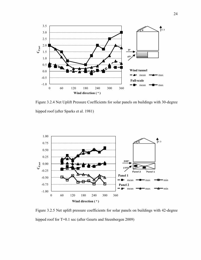
24
Figure 3.2.4 Net Uplift Pressure Coefficients for solar panels on buildings with 30-degree
hipped roof (after Sparks et al. 1981)
Figure 3.2.5 Net uplift pressure coefficients for solar panels on buildings with 42-degree
hipped roof for T=0.1 sec (after Geurts and Steenbergen 2009)
-1.0
-0.5
0.0
0.5
1.0
1.5
2.0
2.5
3.0
3.5
0 60 120 180 240 300 360
CP
,net
Wind direction ( o )
mean max
mean max
Full-scale
Wind tunnel
-1.00
-0.75
-0.50
-0.25
0.00
0.25
0.50
0.75
1.00
0 60 120 180 240 300 360
CP
,net
Wind direction ( o )
mean max min
mean max min
Panel 1
Panel 2

25
Finally, Figure 3.2.6 presents findings from the Stenabaugh et al. (2010) wind tunnel
study. The graph includes results from two building models with roof angles of 30 and 45
degrees respectively. It should be noted that only values obtained from the experiments
with the solar panel located at the center of gable roof building are presented. The
comparison of the peak uplift pressure coefficients for 90, 180 and 270-degree wind
angles show significant differences while for the rest of the examined wind angles, the
results are in better agreement.
Figure 3.2.6 Minimum uplift pressure coefficients for solar panels located at the center of
30- and 45-degree pitched roofs (after Stenabaugh et al. 2010)
-5.0
-4.0
-3.0
-2.0
-1.0
0.0
0 60 120 180 240 300 360
Cp
,net
(m
in)
Wind direction ( o )
θ=30o
θ=45o

26
3.2.3 Solar panels and rooftop equipment near roof edges and corners
Description of Studies
There are a very limited number of studies dealing with wind loads applied on rooftop
equipment and solar panels located at the edges of the roof. Because of the building
geometry, the wind flow pattern will be different near the building edges and will change
closer to the center.
Hosoya et al. (2001) conducted wind tunnel experiments in order to investigate the wind-
induced loads, such as lateral, uplift forces and overturning moment, applied on a cubic
model representing an air conditioner unit placed on top of a building. The geometric
scale selected for this study was 1:50 and the dimensions of their cubic model were
0.0244 m x 0.0244 m x 0.0244 m. A total of 25 pressure taps were installed on the
sidewall and top surfaces of the cubic model. The cubic model was placed at three
different locations in order to examine the wind effect at different distances from the roof
edges.
Another interesting study was conducted by Bronkhorst et al. (2010) which examined the
wind-induced effect on an array of solar panels located at the roof edge of a flat-roof
building. This study included both wind tunnel experiments and numerical simulation.
The solar panels had a depth of 0.024 m (wind tunnel model) and an inclination of 35
degrees while 120 pressure taps were used, located along the solar panels. The building
model was constructed using a 1:50 geometric scale and its dimensions were equal to 0.2
m x 0.6 m x 0.8 m (height x width x length).

27
Similar to the previous study, Bienkiewicz and Endo (2009) performed both wind tunnel
tests and numerical simulations on loose-laid roofing systems. Pressure measurements
were taken at points located at the roof corner region with and without the roofing system
in place. The effect of permeability on the total wind-induced force was also examined.
The results showed that the system permeability -which is also related to the gaps
between the panels- and the flow resistance control the wind uplift reduction under the
system, which corresponds to the spacing under the panel. Finally, as previously
discussed, Erwin et al. (2011) and Saha et al. (2011) performed wind tunnel and full scale
experiments for model configurations in which solar panels are located near roof edges.
A large-scale experimental study was carried out by Erwin et al. (2011) using the 6-fan
Wall of Wind (WoW) facility at Florida International University creating turbulent flow
conditions. A PV module with dimensions 1.57 m x 0.95 m x 0.041 m (length x width x
thickness) was mounted on a flat roof building with dimensions 4.3 m x 4.3 m x 3.2 m.
The PV modules were tested in two different positions; namely “Position 1” at the center
and close to the roof edge and “Position 2” at the corner of the building. However, the
results from this study cannot be compared to this section’s experimental findings since
they apply only for the case in which the panels are located at the roof edge and no other
study discussed data for such configuration.
Last but not least, Saha et al. (2011) tested an array of 18 solar collector models, two of
which were equipped with pressure taps on both the upper and lower surface. The wind
tunnel model was of 1:50 geometric scale and the size of each collector was 0.02 m x
0.04 m. The model was tested in suburban exposure with 0.2 power exponent. The solar
collectors covered the whole roof of the flat roof building model which had dimensions

28
equal to 0.4 m x 0.45 m x 0.45 m (height x width x depth). Several different collector
location configurations were examined such as edge and center areas by changing the
position of the two-instrumented panels.
Experimental Results
Although, Hosoya et al. (2001) and Bronkhorst et al. (2010) examined the wind loads
when the units were placed at the roof edge, the comparison between the results of the
two studies is not possible due to the different model geometry; i.e. inclined panels vs.
cubic attachment. Moreover, the area of the solar panel models is much bigger compared
to that of the cubic model. However, comparisons were made for the studies of Erwin et
al. (2011) and Saha et al. (2011) and are presented in Figure 3.2.7. Several cases for
different inclinations have been included in this comparison and results are presented in
terms of both mean and peak net pressure coefficients.
As far as the Erwin et al. (2011) study is concerned, both mean and peak values follow
the same pattern for 15 and 45 degrees panel inclination. The inclination of the panels has
a minimal effect on the mean values. The absolute minimum and maximum net pressure
coefficients reach their peak for the wind directions of 45 and 135 degrees respectively. It
should be noted that for wind directions greater than 45 degrees, the minimum and
maximum values are really close for the configurations of 15 and 45-degree panel
inclination. On the other hand, Saha et al. (2011) maximum values show a different trend
and are in relative agreement to those of Erwin et al. (2011) only for the case of 0-degree
wind direction. This phenomenon can be attributed to the fact that different geometries
were considered for the building and solar panel models. Moreover, it should be noted

29
that Erwin et al. (2011) performed full-scale experiments while Saha et al. (2011) only
wind tunnel tests.
Figure 3.2.7 Force Coefficients for solar panels located near roof edges (corner position)
3.2.4 Sloped solar panels at the ground level
There are a few studies that have been carried out regarding the wind loads either applied
on single solar collector panels or arrayed panels which are located in the fields. The data
concerning those studies have been collected and presented in this section for inclined
solar collectors at an angle greater than 10 degrees with respect to the flat surface.
-3
-2
-1
0
1
2
3
4
0 60 120 180 240 300 360
CF
,net
Wind direction ( o )
mean max min
mean max min
mean max min
max min
Erwin et al (2011)- 0
Erwin et al (2011)- 15
Saha et al (2011)- 15
Erwin et al (2011)- 45

30
Description of Studies
One very interesting study was conducted by Kopp et al (2002), who performed wind
tunnel experiments on a solar collector system consisting of six parallel slender modules
incorporated in a frame with curved top module surface using a 1:6 scale. The distance
between the modules was 76 mm and the length of the module was 750 mm. The six
wind tunnel scaled modules were equipped with 504 pressure taps in total. The Reynolds
number was 7.6x10⁴. The results were presented in terms of wind uplift pressure
coefficient and the worst cases occurred for 270o and 330
o wind angles. Peak and mean
pressure coefficients were estimated for turbulent flow for 45-degree inclination and 75-
degree module angle.
Wind tunnel experiments were performed by Chung et al (2008) using a 60% scaled,
commercial solar water heater (see Figure 3.2.8), which included a flat panel of 1.2 m x
0.6 m dimensions and a cylinder on top of it with 0.27 m diameter and 0.7 m length. The
flat plate faced the flow direction and was inclined at an angle of 25 degrees, which is
considered the worst case as far as the wind uplift pressure coefficient is concerned and
the one commonly used for solar panels installation in Taiwan. The pressure was
measured on the upper and lower surface of the flat panel by drilling the surface and
placing 26 pressure taps along the centerline of the panel. A closed loop low speed wind
tunnel was employed with constant area test section of 1.2 m high, 1.8 m wide and 2.7 m
long while the turbulence intensity was 0.3% with the wind speed adjusted from 20 m/s
to 50 m/s. Nevertheless, the main goal of the study was to focus on the effect of a steady
wind and as a result, the flow was uniform instead of simulated boundary layer.

31
Figure 3.2.8 Solar water heater (after Chung et al, 2008)
In another study released one year later, again by Chung et al (2009) wind tunnel
experiments were carried out using the same laboratory equipment and therefore the
initial conditions remained the same. They changed, however, their models using a 60%
scaled plate model with a cylinder, a 60% plate model that was only a flat panel and a
40% model with a flat plate panel. Their models were tested for inclinations of 15, 20, 25,
and 30 degrees facing the flow direction.
CFD simulations were carried out by Shademan and Hangan (2009) on stand-alone and
arrayed panels for a set of 3x4 solar panels. Each panel had dimensions 1 m in length, 0.5
m in width and 3 mm thickness with gaps of 0.01 m between two panels. The model
formed, was 22 m in length, 15 m in width and 10 m in height, and was raised 0.6 m
above the ground. The dimensions of the computational domain were 22 m in length,

32
15 m in width and 5 m in height. Two different inclinations (30 and 35 degrees) of the
panel and three wind directions (30, 60, 90 degrees) were simulated in order for the wind
loads to be investigated under different configurations.
More wind tunnel experiments followed by Chung et al (2011) who fabricated a 60%
scaled commercial solar panel (1.2 m x 0.6 m) with horizontal cylinder (0.27 m in
diameter and 0.7 m in length). They tested their model under the same conditions as in
the previous studies, where the maximum blockage ratio was 8.75%. The residential flat
panel under consideration was inclined, with a tilt angle of 15, 20 and 25 degrees
respectively with respect to the flat ground level. The pattern followed for measuring the
pressure on the upper and lower surface of the panel was the same as described in their
previous experiments.
Shademan et al (2010) repeated their CFD simulation for 12 stand-alone panels arrayed
using the same configuration. Four different inclinations (30o, 35
o, 40
o, 50
o) and 7 wind
directions (0o, 30
o, 60
o, 90
o, 120
o, 150
o, 180
o) were simulated. The dimensions of the
computational domain are 30 m in length, 21 m in width and 10 m in height while the
Reynolds number under which the simulation was conducted is Re = 2x10⁶. By testing all
the different configurations described, it was found that the worst wind loads occurred for
0 and 180 degrees.
Two different methods used by Bitsuamlak et al (2010) tried to investigate the
aerodynamic characteristics of panels located on the ground under boundary layer effect.
The study included both computational simulations and full-scale experiments. For the
numerical simulation, a typical panel of 1.3 m height was considered with inclination of

33
40 degrees. The angle of attack was 0, 30 and 180 degrees. The full-scale experiments
took place at Florida International University and the wind uplift pressure coefficients on
the panels were determined. The 11 pressure taps used, were located along a vertical line
on the upper and lower surface of the panels. The dimensions of the panels were 1.3 m
x1.1 m x0.019 m (length x width x depth) and they were attached to a frame inclined by
40 degrees angle while the incidence wind angle could take the values 0 and 180 degrees.
Meroney and Neff (2010) carried out some numerical calculations and wind tunnel
experiments to estimate the uplift coefficient on solar collectors for 2-D and 3-D flow
patterns using ½ scale models, which were inclined by 10 degrees with respect to the flat
roof. They used eight additional dummy tiles so as an array 3x3 in size could be installed
in the 1.8 meters wide wind tunnel.
Experimental Results
A summary of the experimental and simulation results for stand-alone solar panels
inclined by an angle ranging from 10 to 25 degrees is shown in Table 3.2.1.
According to Meroney and Neff (2010) results, it can be said that for 10o inclination, the
net uplift pressure coefficient is greater for 180o wind angle compared to the 0
o wind
direction.
Chung et al (2008, 2009) experiments seem to be in agreement since only small
differences can be observed concerning their examined model which is fabricated in a
60% scale. In addition, as the inclination gets greater values, the suction increases since
its absolute value becomes greater.

34
Wind Direction 0o
180o
Meroney and Neff (2010) 10o inclination
CFD- 2D -0.04 -0.183
Measured- 2D 0.07 -0.073
CFD- 3D -0.02 -0.1
Measured- 3D 0.07 -0.07
Chung et al (2008), 25o inclination -1.1
Chung et al (2009)
Case B, 15o inclination -0.6
Case C, 15o inclination -0.4
Case B, 20o inclination -0.8
Case C, 20o inclination -0.6
Case B, 25o inclination -1
Case C, 25o inclination -0.8
Chung et al (2011)
15o inclination -0.8
20o inclination -1.0
25o inclination -1.1
Case B: 60% scaled model with a flat panel only
Case C: 40% scaled model with a flat panel only
Table 3.2.1 Stand-alone solar panels inclined by a 10 to 25 degrees angle

35
Figure 3.2.9 depicts the results for solar panels inclined by a 30 and 35 degrees slope.
From this Figure, it can be observed that the uplift pressure coefficient takes only positive
values when CFD methods apply. Therefore, the results coming out of Shademan and
Hangan (2009, 2010) and Chung et al (2009) take values with opposite signs for 180
degrees wind angle. It can be seen that Shademan’s CFD results are not in good
agreement either and the only differences between the two studies is the computational
domain considered.
Figure 3.2.9 Net uplift pressure coefficient for solar panels inclined by 30 and 35 degrees
angle on the ground level
However, it is necessary to mention that the results shown in Figure 3.2.9 are the values
of the wind uplift pressure coefficients corresponding to those values recorded at the
-2
-1.5
-1
-0.5
0
0.5
1
1.5
2
0 60 120 180 240 300 360
Cp
,net
(m
ean
valu
es)
Wind direction ( o )
30 35
30 35
case B case C
Shademan and Hangan
(2010)
Shademan and Hangan
(2009)
Chung et al (2009) - 30o

36
middle of the flat solar panels. The particular location was selected because in some
cases, the pressure coefficient is provided only along the centerline and therefore
comparison can be feasible among different studies.
Figure 3.2.10 presents the results for solar panels inclined by a 40 to 50 degrees angle.
Bitsuamlak et al (2010) study shows that their experimental results, although two
different methods were used (full scale experiments and CFD simulations), are in good
agreement. For wind angles in the range of 0 to 60 degrees wind angle Shademan and
Hangan’s results agree with those of Bitsuamlak. However, for a wind angle 180o, the
uplift pressure coefficient takes positive values for Shademan and Hangan study while for
Bitsuamlak are negative.
Figure 3.2.10 Net Uplift Pressure Coefficient for solar panels inclined by a 40-50 angle at
the ground level
-2
-1.5
-1
-0.5
0
0.5
1
1.5
2
2.5
3
0 60 120 180 240 300 360
Cp
,net
(m
ean
)
Wind direction ( o )
40 50
WOW CFD
45
Bitsuamlak et al (2010)- 40o
Shademan and Hangan (2010)
Kopp et al (2002)

37
CHAPTER 4: WIND TUNNEL STUDY
4.1 GENERAL
Wind tunnel experiments play a very important role in determining the wind loads
applied on structures. This chapter summarizes and describes all the necessary
information related to wind tunnel testing such as the wind tunnel facilities, the boundary
layer simulation, as well as, the models constructed and tested. Moreover, the equipment
used, the wind tunnel experimental method, the data analysis procedure and finally the
repeatability tests are also presented in this chapter.
4.2 WIND TUNNEL FACILITIES
The experiments described in this chapter took place at the Building Aerodynamic
Laboratory located at the Engineering Building of Concordia University. The type of the
wind tunnel falls in the category of an open circuit, blowdown tunnel having a working
area 12 m long and cross-section 1.8 m wide and height ranging from 1.4 m to 1.8 m - see
Figures 4.2.1 and 4.2.2. Models are usually located into the downstream section on a
turntable of 1.21 m diameter which can operate manually or electrically and allows
models to be tested for different wind attack angles. The wind speed can range from 3
m/s to 14 m/s inside the wind tunnel section.
The floor of the working section in the wind tunnel is covered with a certain type of
carpet which is used to simulate the open country terrain. For different terrain types to be
simulated, roughness elements are added on panels which can be inserted in the wind

38
tunnel test section. Additional details for the wind tunnel construction and characteristics
are given by Stathopoulos (1984).
Figure 4.2.1 The Boundary Layer Wind Tunnel of Concordia University after
Stathopoulos (1984)
Figure 4.2.2 Front View of the Boundary Layer Wind Tunnel with the building model in
position

39
4.3 ATMOSPHERIC BOUNDARY LAYER
It is really crucial when performing wind tunnel experiments for building testing to
accurately simulate the atmospheric boundary layer wind velocity profile. As has already
been mentioned in a previous chapter, wind fluctuates randomly and this is the reason
why it is characterized as turbulent. The floor of the atmospheric boundary layer wind
tunnel of Concordia University is covered by carpet and thus is classified by default in
the open terrain category.
Before starting with the experiments, the velocity wind profile had to be checked without
the test model in its position. More specifically, the wind speed was measured at the
center of the wind tunnel section at different heights. Figure 4.3.1 gives the curve of the
wind speed measured at different heights as a function of the height in comparison with
the theoretical curve resulting from the power law when α = 0.16. Figure 4.3.2 presents
the turbulence intensity profile which is 17.65% at the top of the 7 m high building and
13.9% at the top of the 16 m high building.

40
Figure 4.3.1 Wind velocity profile
Figure 4.3.2 Turbulence intensity profile
4.4 BUILDING AND SOLAR PANEL MODEL
A geometrical scale 1:200 was selected, considering the similarity parameters that must
be satisfied when performing wind tunnel tests. A sophisticated model was constructed so
as to simulate a prototype building as realistically as possible. The model consists of a
rectangular building model on top of which three identical panels were attached. Both
panels and building model were constructed under 1:200 scale. Transparent plastic was
used for the fabrication of the walls having a thickness of 10 mm at the front and back
walls and 3 mm at the side walls, while the roof and the panels were metallic. The
external dimensions of the building model were 15.3 cm (length) x 9.8 cm (width), while
0
0.1
0.2
0.3
0.4
0.5
0.6
0.7
0.8
0.9
1
0 0.2 0.4 0.6 0.8 1
Z/Z
g
V/Vg
WT profile
V/Vg= (Z/Zg)^α,
α=0.16
0
0.1
0.2
0.3
0.4
0.5
0.6
0.7
0.8
0.9
1
0 0.2 0.4 0.6 0.8 1 Z
/Zg
Vrms/Vz
WT profile

41
the height corresponding to two different cases was 3.5 cm and 8 cm respectively (Figure
4.4.1).
Figure 4.4.1 Elevation of building models with inclined solar panels attached
Three similar panels were mounted on the building roof. Their dimensions were 4.3 cm
(length), 2.8 cm (width) and 1 mm (thickness). The panels were located in two different
positions on the roof, the one closer to the side facing the 0o wind direction and the other
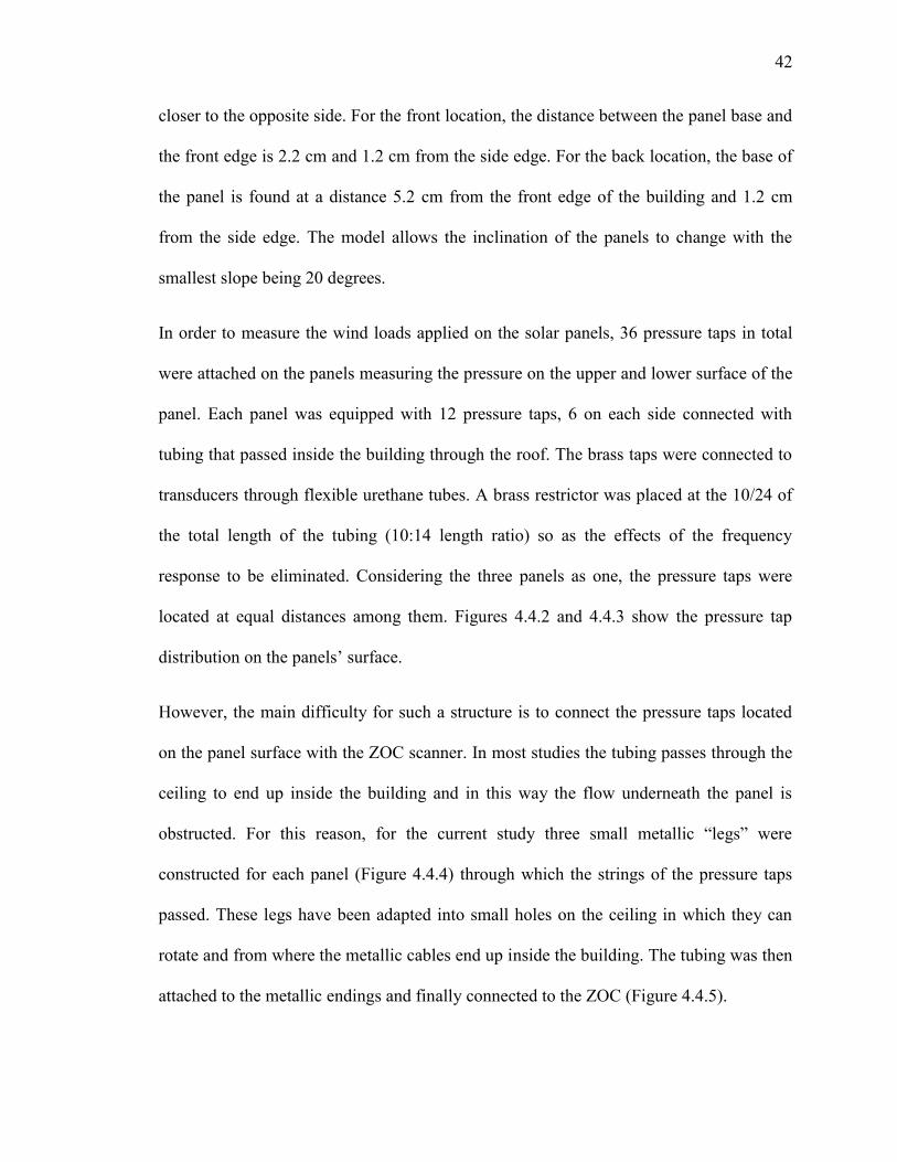
42
closer to the opposite side. For the front location, the distance between the panel base and
the front edge is 2.2 cm and 1.2 cm from the side edge. For the back location, the base of
the panel is found at a distance 5.2 cm from the front edge of the building and 1.2 cm
from the side edge. The model allows the inclination of the panels to change with the
smallest slope being 20 degrees.
In order to measure the wind loads applied on the solar panels, 36 pressure taps in total
were attached on the panels measuring the pressure on the upper and lower surface of the
panel. Each panel was equipped with 12 pressure taps, 6 on each side connected with
tubing that passed inside the building through the roof. The brass taps were connected to
transducers through flexible urethane tubes. A brass restrictor was placed at the 10/24 of
the total length of the tubing (10:14 length ratio) so as the effects of the frequency
response to be eliminated. Considering the three panels as one, the pressure taps were
located at equal distances among them. Figures 4.4.2 and 4.4.3 show the pressure tap
distribution on the panels’ surface.
However, the main difficulty for such a structure is to connect the pressure taps located
on the panel surface with the ZOC scanner. In most studies the tubing passes through the
ceiling to end up inside the building and in this way the flow underneath the panel is
obstructed. For this reason, for the current study three small metallic “legs” were
constructed for each panel (Figure 4.4.4) through which the strings of the pressure taps
passed. These legs have been adapted into small holes on the ceiling in which they can
rotate and from where the metallic cables end up inside the building. The tubing was then
attached to the metallic endings and finally connected to the ZOC (Figure 4.4.5).

43
Figure 4.4.2 Pressure tap distribution on the solar panel surface
Figure 4.4.3 Top view of the building roof with solar panels attached and pressure tap
notation

44
Figure 4.4.4 Detailed view of the solar panel “legs”
Figure 4.4.5 View of the pressure tap tubing
The building model was located on the turntable as illustrated in Figure 4.4.6 which can
rotate 360 degrees and allows different wind attack angles to be tested. The building base
that was set in the turntable allowed the building movement upwards and downwards so
that the wind loads applied on the panels could be examined for different building
heights.
45
Since the environment plays an important role for the flow, it needs to be clarified that
the experiments were conducted for the case of an open terrain simulation. Additionally,
sharp edges and corners on the building and panel models are really important for the
flow separation to occur. In this way, kinematic and dynamic similarities can be assured
even if the Reynolds number of the model is not the same as that for the prototype.
Figure 4.4.6 View of building model with panels placed on the turntable at 135o wind
direction
46
4.5 EQUIPMENT
This section presents the sophisticated instrumentation with which the wind tunnel is
equipped. Figure 4.5.1 shows how the instruments are connected. The measurements of
wind speed and turbulence intensity profile were conducted using the 4-hole Cobra
probe. A 1000 Hz sampling rate was used for the velocity measurements and 30 seconds
was the duration of each run. For the open terrain, the gradient mean wind velocity was
approximately 13.6 m/s.
A sensitive pressure scanning system was used for pressure measurements. This system
consists of a Digital Service Module (DSM 3400) and one pressure scanner ZOC33/64Px
from Scanivalve. The DSM can be connected with up to 8 ZOC pressure scanners and
through Ethernet all the output data can be transferred to a computer. A ZOC module can
host up to 64 pressure sensors. Its temperature has to be maintained constant and this is
why it is kept inside an insulated thermal unit. For the current experiment 36 pressure
taps were connected through urethane tubing to the ZOC which in turn was connected to
the DSM unit. The DSM system was scanning every 50 μs and as a result the sampling
frequency was 312.5 Hz. In total, 8200 frames were scanned which means that the
duration for each run was 26.25 sec. The output data acquired during the scanning
process was in binary format and Ethernet connection was used for the transfer.

47
Figure 4.5.1 Sketch of the experimental wind tunnel equipment (after Zisis 2006)
4.6 WIND TUNNEL TESTS
For the experiments performed, the 36 pressure taps of the panels were connected to a
ZOC module. A cable connected the ZOC module with the DSM unit and then the signals
were transferred to a host computer. This computer is equipped with two software: DSM-
Link which measures scans of low and moderate frequencies and Btel for higher
frequencies.
The building model with the panels attached is symmetrical and for this reason the wind
direction ranged from 0 to 180 degrees while a total number of 13 wind attack angles
were tested with 15 degree intervals. The model can also be tested for different panel
inclinations and for the present study the panel angles tested were 20, 30, 40 and 45
degrees.
The experimental procedure followed is described below:
Choose and set the panel inclination examined
Set all the panels at the same inclination

48
Set the building at 0o wind direction (facing the wind tunnel fan)
Provide compressed air in the tubing
Run DSM-Link and perform a zero calibration for all the channels
Turn on the wind tunnel fan
Open B-Tel file, scan, close and save the file
Change the direction of the turntable and continue the same procedure for 15o
increments for wind direction ranging from 0-180 degrees
Turn off the wind tunnel fan
Repeat zero calibration
The zero calibration was performed so as the drift of the sensors measuring the pressure
to be estimated and corrected. The files were all saved with two characteristic numbers,
one indicating the panel slope and the other the wind attack angle.
In total four rounds of measurements took place, each one for different panel slope and
for 13 different wind directions with 15 degree intervals.
4.7 DATA ANALYSIS
The mean and peak pressure coefficients have been derived by applying dimensional
analysis. The following formulas have been used:
(4.1)
(4.2)

49
The units that have been used for the above equations are kPa for the pressure, m/s for the
wind speed and kg/m3 for the air density. The measurements of the pressure are given in
binary format from the software. The procedure followed was the same for all the cases
and is described below:
Import the record of the pressure scanned for all wind attack angles for each slope
Import the record of the error-drift for each case
Subtract the corresponding drift values for each channel
In order to estimate the Cp values, it is necessary to know the dynamic pressure at the
building height. Using the power law for α = 0.16 at the gradient height h = 70 cm and
knowing the building height for each case, the dynamic pressure at building height is
acquired. A division of the corrected pressure value with the dynamic pressure at building
height gives the pressure coefficient. More specifically, for the mean pressure
coefficients, the average value of the estimated pressure coefficient for each channel is
calculated, whereas, for the peak pressure coefficients the average value of the ten
maximum and ten minimum values are computed for each channel.
The force coefficients for each panel, considering that the area corresponding to each
pressure tap was approximately equal, were calculated by adding the net local pressure
coefficients and then dividing by the number of the pressure taps.
Basically, the output data has a signal form as depicted in Figure 4.7.1. It is this signal
that is corrected accordingly and transformed so as the pressure and force coefficients to
be acquired. The signal of Figure 4.7.1 corresponds to the pressure tap number 1, when
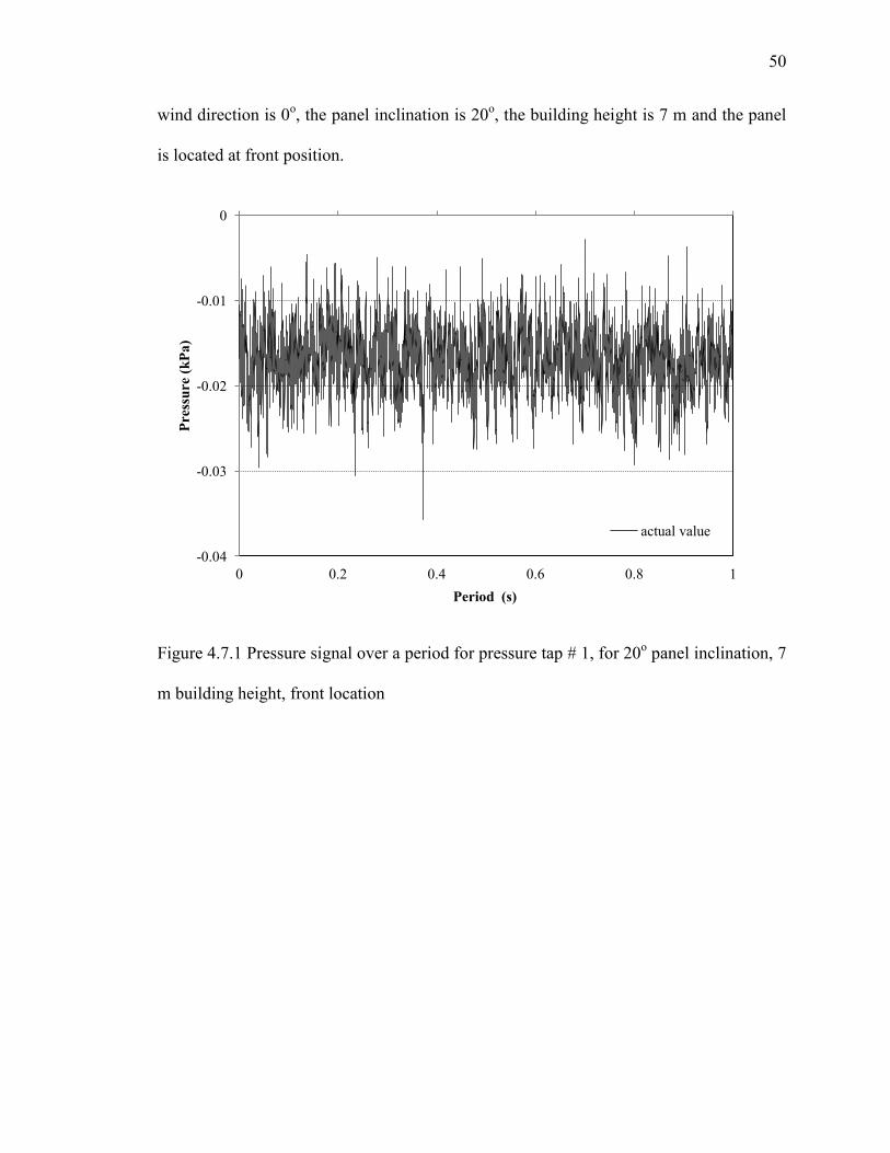
50
wind direction is 0o, the panel inclination is 20
o, the building height is 7 m and the panel
is located at front position.
Figure 4.7.1 Pressure signal over a period for pressure tap # 1, for 20o panel inclination, 7
m building height, front location
-0.04
-0.03
-0.02
-0.01
0
0 0.2 0.4 0.6 0.8 1
Pre
ssu
re (
kP
a)
Period (s)
actual value

51
4.8 REPEATABILITY OF DATA
During the experimental process, it is really important to confirm the validity of the
experimental results. Therefore, two identical experiments took place with eleven days
difference. The model was tested for the case of 16 m building height, 20o panel
inclination, with panels located at front position for all wind directions. As depicted in
Figure 4.8.1 both experiments show almost identical experimental results as far as the
mean and peak pressure coefficients are concerned. The fact that the data shows good
repeatability can be further used so as to reassure that the experimental instruments and
equipment function properly and provide valid data.
Figure 4.8.1 Repeatability of data for mean and peak net pressure coefficients for panel
(pressure tap #1) attached to 16 m building height, 20o panel inclination, front location
and 0o wind direction
-5
-4
-3
-2
-1
0
1
2
0 30 60 90 120 150 180
Cp
,net
Wind direction ( o )
mean min max
mean min max
29 - Sep
10 - Oct

52
CHAPTER 5: RESULTS AND DISCUSSION
5.1 GENERAL
The output data after the completion of the wind tunnel experiments were all organized in
different sections in this chapter so as the effect of different parameters to be shown and
discussed. The experiments were performed for two different building heights and two
different panel locations; namely front (closer to the building edge facing the 0o wind
direction – see Figure 5.1.1) and back (closer to the opposite edge – see Figure 5.1.2). In
addition, a third configuration was examined, for panels located at ground level – see
Figure 5.1.1). Moreover, thirteen different wind directions were examined starting from
0o to 180
o with 15
o intervals and four different panel inclinations namely 20-, 30-, 40-,
45- degrees. A selection of the most critical cases are presented in this chapter, additional
data are shown in Appendices A and B.

53
Figure 5.1.1 Top and side building views with front panel configuration
Note: Odd numbers correspond to the upper panel surface while even numbers to the
lower panel surface.

54
Figure 5.1.2 Top and side building views with back panel configuration

55
Wind tunnel experiments produced a wide range of data which were further analyzed so
as to better understand the wind-induced response of these structures. The values of mean
and peak pressure coefficients were all evaluated for individual set of taps on solar panels
corresponding either on the upper or the lower panel surface. Moreover, the net pressure
coefficients were calculated by considering simultaneously the upper and lower surface
pressure traces. Calculation of net pressure coefficients for individual set of taps on solar
panels shows that minimum values are more critical since in terms of absolute values are
greater compared to those of the maxima. Further investigation of the acquired data can
provide information for the exact location at which extremes occur as well as for their
magnitude.
This kind of information concerning the exact location is provided in Table 5.1.1 which
summarizes the pressure tap numbers for which the most extreme values of the net
minima are observed. It should be noted that all tested wind directions were considered as
well as all model configurations. The grey-coloured boxes indicate for which wind
direction the most extreme values occur, while the number in the grey boxes corresponds
to the pressure tap. Clearly, the most critical minima do occur for wind directions ranging
from 120o to 165
o and especially for 135
o wind direction for which most configurations
get their peak value. Along with 135o wind direction, pressure tap number 1 is
experiencing the greatest pressure.
The most critical case, in terms of net pressure coefficients, is for approaching wind
direction 135 degrees. For this reason, detailed contour plots have been drawn for wind
direction 135o so as the most typical and at the same time critical results to be presented.
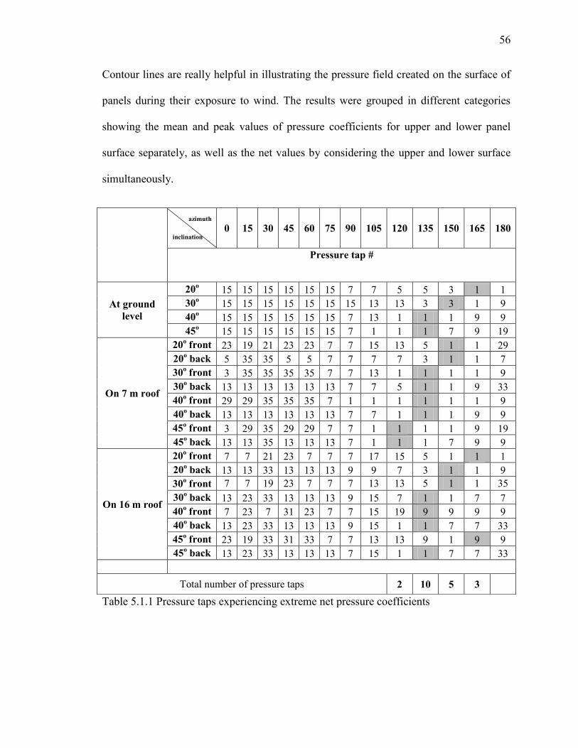
56
Contour lines are really helpful in illustrating the pressure field created on the surface of
panels during their exposure to wind. The results were grouped in different categories
showing the mean and peak values of pressure coefficients for upper and lower panel
surface separately, as well as the net values by considering the upper and lower surface
simultaneously.
Table 5.1.1 Pressure taps experiencing extreme net pressure coefficients
azimuth
inclination 0 15 30 45 60 75 90 105 120 135 150 165 180
Pressure tap #
At ground
level
20o
15 15 15 15 15 15 7 7 5 5 3 1 1
30o
15 15 15 15 15 15 15 13 13 3 3 1 9
40o
15 15 15 15 15 15 7 13 1 1 1 9 9
45o
15 15 15 15 15 15 7 1 1 1 7 9 19
On 7 m roof
20o front 23 19 21 23 23 7 7 15 13 5 1 1 29
20o back 5 35 35 5 5 7 7 7 7 3 1 1 7
30o front 3 35 35 35 35 7 7 13 1 1 1 1 9
30o back 13 13 13 13 13 13 7 7 5 1 1 9 33
40o front 29 29 35 35 35 7 1 1 1 1 1 1 9
40o back 13 13 13 13 13 13 7 7 1 1 1 9 9
45o front 3 29 35 29 29 7 7 1 1 1 1 9 19
45o back 13 13 35 13 13 13 7 1 1 1 7 9 9
On 16 m roof
20o front 7 7 21 23 7 7 7 17 15 5 1 1 1
20o back 13 13 33 13 13 13 9 9 7 3 1 1 9
30o front 7 7 19 23 7 7 7 13 13 5 1 1 35
30o back 13 23 33 13 13 13 9 15 7 1 1 7 7
40o front 7 23 7 31 23 7 7 15 19 9 9 9 9
40o back 13 23 33 13 13 13 9 15 1 1 7 7 33
45o front 23 19 33 31 33 7 7 13 13 9 1 9 9
45o back 13 23 33 13 13 13 7 15 1 1 7 7 33
Total number of pressure taps 2 10 5 3

57
5.2 EFFECT OF PANEL INCLINATION ON MEASURED PRESSURE
COEFFICIENTS
One of the most interesting aspects of the present study is the illustration of the pressure
field using contour plots. These plots are representative of the field created because of
panels’ exposure to wind. The wind angle 135o is the most critical and for that reason, the
pressure fields have all been plotted for this wind direction. The numbers along the
contour lines denote the magnitude of mean and peak pressure coefficients. The mean
values of pressure coefficients, which correspond to upper, lower surface and the net
values are first depicted for panels attached to 7 m-high building and front located; the
minima and maxima of pressure coefficients follow.
Figures 5.2.1, 5.2.2 and 5.2.3 present the mean upper, lower surface and net pressure
coefficients respectively, for 20-, 30-, 40- and 45- degree inclination and for panels at the
front location of the 7 m-high building.
As demonstrated in Figure 5.2.1, suction occurs for all panel inclinations on the upper
surface of the solar panels. Contour lines, however, become less dense with increasing
inclination and as a result, suction is smaller. The greatest suction is observed for 20o and
30o panel inclination at the upper part of panel 1 for both cases.
Positive mean pressure coefficients are measured for lower panel surface, which vary
slightly with panel inclination as depicted by contour lines in Figure 5.2.2. However,
slight suction occurs at the edges of panel 1 and panel 3, which diminishes with
increasing panel inclination. This phenomenon might be caused because of flow
separation that happens near panel edges.

58
Figure 5.2.1Mean Cp values on upper surface for 7 m building height, front location and
135o wind direction

59
Figure 5.2.2 Mean Cp values on lower surface for 7 m building height, front location and
135o wind direction

60
Figure 5.2.3 Net mean Cp values for 7 m building height, front location and 135o wind
direction

61
Combination of the two previous contour maps results in Figure 5.2.3 in which net values
of the pressure coefficients offer the overall suction (negative sign) applied on the solar
panel. Contour lines indicate that panel 1 is mostly affected by the wind since the field
becomes more complex over its surface, while the field over panels 2 and 3 consists of
almost parallel contour lines of, generally, smaller values. It is also evident that
increasing panel inclination results in decreasing net pressure coefficients due to lower
pressure exerted on them. The greatest suction detected, occurs at the upper edge of panel
1 for panel inclination 30o, which slightly differs from the values recorded for 20
o panel
inclination.
As far as the peak values are concerned, Figures 5.2.4 to 5.2.9 demonstrate the resulting
net pressure coefficient derived by combining simultaneously the pressure coefficients
applied on upper and lower surfaces.
Minimum Cp values observed on the upper surface of the panel are illustrated in Figure
5.2.4 which shows that suction occurs for all inclinations. According to this figure,
greatest suction appears for 30o panel inclination at the upper corner of panel 1 near to the
edge, which is greater compared to the peaks occurring for other panel inclinations.
Contour lines also indicate that suction does not change significantly for panels 2 and 3
when they are inclined by 20, 40 and 45 degrees.

62
Figure 5.2.4 Minimum Cp values on upper surface for 7 m building height, front location
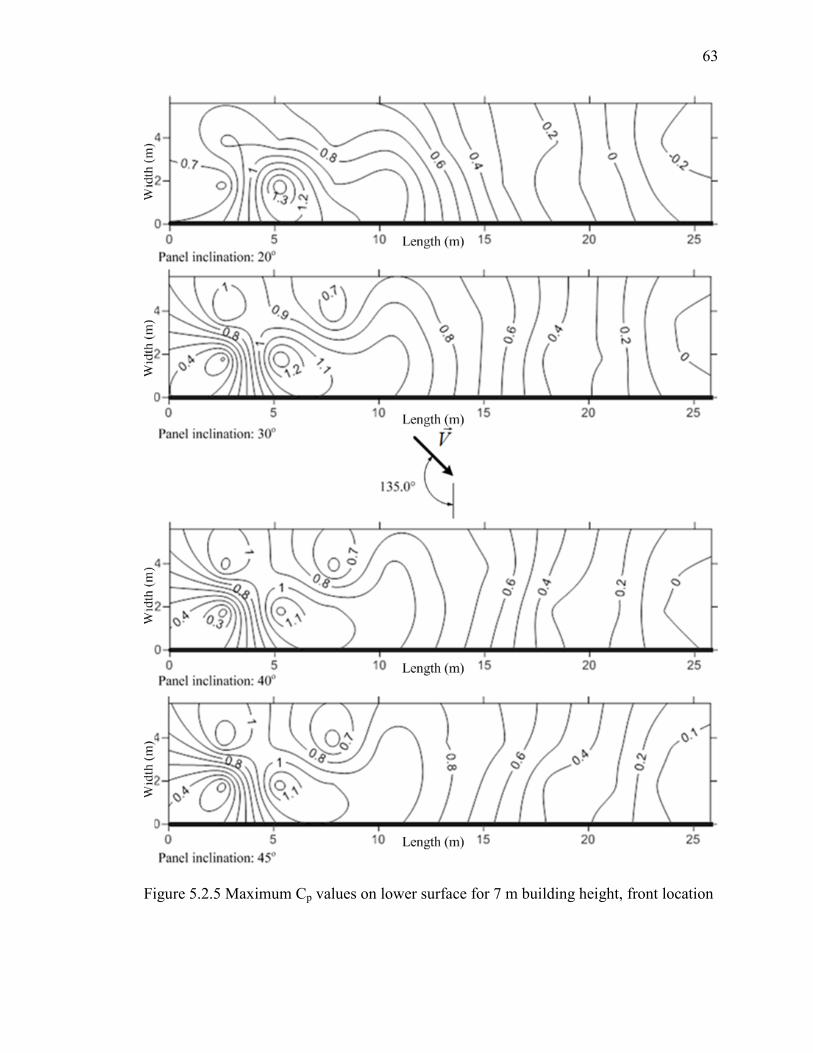
63
Figure 5.2.5 Maximum Cp values on lower surface for 7 m building height, front location

64
Figure 5.2.6 Minimum net Cp values for 7 m building height, front location

65
Figure 5.2.7 Maximum Cp values on upper surface for 7 m building height, front location

66
Figure 5.2.8 Minimum Cp values on lower surface for 7 m building height, front location

67
Figure 5.2.9 Maximum net Cp values for 7 m building height, front location

68
Figure 5.2.5 depicts the maximum values of the pressure coefficients corresponding to
the lower surface of the panel. Contour lines clearly show that overpressure appears all
over the surface of the panels for all the panel inclinations. The extreme value of the
positive pressure coefficients is recorded for 20o panel inclination at the lower edge of
panel 1. As far as panels 2 and 3 are concerned, the pressure field corresponding to them
remains almost constant and unaffected by the panel inclination.
The upper and lower surface panel pressure fields are combined and the resulting field
appears in Figure 5.2.6 which demonstrates that suction is applied on the entire surface of
the panels. Since contour lines at the lower surface don’t change radically with panel
inclination, the contour lines in Figure 5.2.6 follow the same pattern with that of the
upper surface. Therefore, it can be concluded that the pressure field above panel 1 is
mostly affected by the wind flow while panels 2 and 3 appear almost under the same field
for all the panel inclinations. As has already been shown, greater panel inclination results
in lower suction with only exception being the 30o panel inclination for which the
extreme value appears around pressure tap number 1 near the edge of panel 1, where the
extreme values for the other panel inclinations can also be detected.
Figure 5.2.7 shows the maximum values of the pressure coefficients occurring at the
upper surface while Figure 5.2.8 shows the minima at the lower surface from where it is
clear that suction appears for both of them. Contour lines become less dense when panel
inclination increases showing that suction becomes lower. Additionally, maximum values
of Cp corresponding to the upper surface are slightly greater in terms of absolute value
compared to the minimum values of lower surface, indicating that greater suction occurs
at the upper surface.

69
Figure 5.2.9 presents the net pressure coefficients which were calculated by
simultaneously adding the two traces as measured at the upper and lower panel surface.
The resulting pressure fields as depicted in Figure 5.2.9 show that only suction occurs
which varies slightly with panel inclination, particularly for 20-degress panel inclination.
Additional contours corresponding to different configurations have been plotted for the
most critical cases and are available in Appendix A.
As mentioned in Chapter 4, in order to investigate the effect of panel inclination, a
careful study of measured pressure coefficients for several configurations is necessary
and this is presented in this section.
The data are given as a function of the panel inclination for the critical 135o wind
direction. It should be noted that only the extreme values have been considered for the
cases of stand-alone panels and panels attached to buildings. For the cases of the attached
panels on buildings, both building heights (i.e. 7 m and 16 m) and both panel locations
(i.e. front and back) are presented.
For the upper surface, the data are depicted in Figure 5.2.10 (a) in which the maximum
Cp values follow the same pattern for all the panel inclinations while minimum values
vary with different inclination. The pressure coefficients corresponding to the trends for 7
m and 16 m front location decrease with increasing inclination while those corresponding
to the back location increase with increasing inclination. For the stand-alone-panels,
increase of the panel inclination leads to greater suction and consequently the peak
appears for 45o panel inclination which is overall the greatest suction.

70
Figure 5.2.10 (b) shows what happens at the lower panel surface for 135o wind angle and
all the configurations. The minimum and the maximum values of pressure coefficients
differ slightly for different building heights and panel locations. However, the greatest
suction occurs for panels on the 16 m high building, back located and inclined by 20
degrees, while the positive greatest value of the pressure coefficient for the 7 m high
building, at the back location and 20o panel inclination.
The net values of the pressure coefficients referring to the whole solar panel appear in
Figure 5.2.11. The maximum Cp values decrease somewhat with increasing panel
inclination (from -0.5 to < -1.0). On the contrary, the minimum values show smaller
suction with increasing panel inclination for both 7 m and 16 m building height and front
location. The trends for back location show that increasing inclination results in higher
suction for every building height and the stand-alone case as well. The different behavior
for front and back panels comes from the fact that different panel locations affect
differently the wind flow. Panel inclination also contributes to this phenomenon and a
different pressure field is created for different panel inclinations.

71
Figure 5.2.10 Peak pressure coefficients on (a) upper and (b) lower surface for 135o wind
direction
-5
-4
-3
-2
-1
0
1
2
20 25 30 35 40 45
Cp
,pea
k
Panel Inclination ( o )
-5
-4
-3
-2
-1
0
1
2
20 25 30 35 40 45
Cp
,pea
k
Panel Inclination ( o )
(a) upper
(b) lower

72
Figure 5.2.11 Net peak pressure coefficients for 135o wind direction
5.3 EFFECT OF BUILDING HEIGHT ON MEASURED PRESSURE
COEFFICIENTS
Different model configurations were tested in order to evaluate the effect of building
height on the wind-induced load on solar panels. Figures 5.3.1 and 5.3.2 show how the
local peak pressure coefficients from all pressure taps corresponding to different panel
inclinations vary with building height for the most critical case of 135o wind direction.
The peak pressure coefficients for front located panels are depicted in Figure 5.3.1 for
the upper, lower panel surface and the net values. Figure 5.3.1(a) shows that increasing
-5
-4
-3
-2
-1
0
1
20 25 30 35 40 45
Cp
,pea
k (
net
)
Panel inclination ( o )
0m 7m 16m 7m 16m
0m 7m 16m 7m 16m
Front Back
Minima
Maxima

73
building height results in lower suction for every panel inclination. On the contrary, the
suction is smaller for the case of stand-alone panels and for 20o panel inclination. As far
as the lower surface of the panel is concerned, the minima and maxima of pressure
coefficients trends for front location and 135o wind direction follow the same pattern as
shown in Figure 5.3.1(b). Overall, slightly greater suctions do occur when the building
height increases.
Figure 5.3.1(c) depicts the net values of peak pressure coefficients as a function of
building height. Maximum values range from -1.2 to -0.2 as a function of the building
height. As far as the minima are concerned, the 16 m high building results in lower
suctions for every panel inclination compared to those appearing for 7 m high building.
For panels at the ground level, suction takes its greatest value for 40o and 45
o panel
inclination, while the lowest suction appears for 20o panel inclination. The trend of 30
o
panel inclination ranges from -4.2 to -3.7 and thus no significant building height effect is
observed
.

74
Figure 5.3.1 (a) upper, (b) lower surface peak pressure coefficients and (c) net peak
pressure coefficients for front location and 135o wind direction
-6
-5
-4
-3
-2
-1
0
1
2
0 2 4 6 8 10 12 14 16
Cp
,pea
k
Building height (m)
-6
-5
-4
-3
-2
-1
0
1
2
0 2 4 6 8 10 12 14 16
Cp
,pea
k
Building height (m)
-6
-5
-4
-3
-2
-1
0
1
2
0 2 4 6 8 10 12 14 16
Cp
,pea
k
Building height (m)
(a) upper
(b) lower
(c) net

75
Figure 5.3.2 (a) upper, (b) lower surface peak pressure coefficients and (c) net peak
pressure coefficients for back location and 135o wind direction
-6
-5
-4
-3
-2
-1
0
1
2
0 2 4 6 8 10 12 14 16
Cp
,pea
k
Building height (m)
-6
-5
-4
-3
-2
-1
0
1
2
0 2 4 6 8 10 12 14 16
Cp
,pea
k
Building height (m)
-6
-5
-4
-3
-2
-1
0
1
2
0 2 4 6 8 10 12 14 16
Cp
,pea
k
Building height (m)
(a) upper
(b) lower
(c) net

76
For the back location, as depicted in Figure 5.3.2(a) and in which the peak pressure
coefficients appear for the upper surface, the trends remain almost constant for both
building heights and stand-alone panels.
Figure 5.3.2(b) demonstrates the peak pressure coefficients at the lower surface for back
location and 135o wind direction from which can be concluded that increasing building
height results in higher suction in total. Maximum values are almost constant and remain
within the same range.
Finally, the net values of pressure coefficients for the critical 135o wind direction and
back location are depicted in Figure 5.3.2(c). The results show that there are differences
compared to Figure 5.3.1(c) indicating that panel location plays an important role
especially as far as the minimum pressure coefficients are concerned. The trends for the
minimum values of 30-, 40- and 45- degree panel inclination range from -4.6 to -3.7
while the one of 20-degree panel inclination takes values from -2.9 to -2.1. Further
comparison between the two figures also makes evident the fact that absolute values of
minimum pressure coefficients are greater for the back location and their range is within -
5 and -4 for 30-, 40-, 45- degree panel inclination.

77
5.4 EFFECT OF PANEL LOCATION AND WIND DIRECTION ON NET
PEAK PRESSURE COEFFICIENTS
This section presents the effect of wind direction and panel location on experimental
results expressed as net peak pressure coefficients. Figures 5.4.1 to 5.4.2 demonstrate
how the net peak pressure coefficients vary as a function of wind direction for stand-
alone panels and panels attached to 7 m and 16 m high building when panels are inclined
by 20-, 30-, 40-, 45- degrees. Moreover, Figures 5.4.2(a) and 5.4.2(b) illustrate the results
for both front and back panel location. In general, the following comments can be made
for these figures:
As far as the minimum values are concerned, higher suction occurs for wind
directions ranging from 120o to 165
o. On the other hand, maximum value
extremes appear within the range of 15o to 60
o of wind direction.
Building height increase results in greater suction.
Back location is mainly responsible for greater suction while front location is
responsible for slightly greater overpressure.
Overall, overpressure is not as significant as suction in terms of absolute values.
More specifically, Figure 5.4.1 shows the peak pressure coefficients for the case of stand-
alone panels for the panel inclinations examined. The peaks appear for 30o and 135
o wind
directions for the maximum and the minimum values respectively. It is also evident that
suction is greater than overpressure in absolute value.

78
Figure 5.4.1 Net peak pressure coefficients for ground level panels with respect to wind
direction
The case where the panels are attached to a 7 m high building, located at the front and
back of the roof is shown in Figure 5.4.2(a). For wind directions 120o and 135
o the
extreme values do occur for 45- and 30- degree panel inclination respectively, when the
panel is back located. The maximum positive pressure can be observed for 30o wind
direction when the panels are located at the front position and are inclined by 45o.
Figure 5.4.2(b) presents the case where the panels are attached to a 16 m high building
from which can be concluded that suction is overall greater than overpressure in terms of
absolute values. In addition, greater suction appears for back located panels while
overpressure is greater for front located panels. These phenomena can be attributed to the
flow separation occurring due to the sharp building edges. The greatest suction occurs for
135o wind direction when the panel location is back, and the panel inclination is 30
-6
-5
-4
-3
-2
-1
0
1
2
3
4
0 15 30 45 60 75 90 105 120 135 150 165 180
Cp
, p
eak
(n
et)
Wind direction ( o ) 20 30 40 45
20 30 40 45
Minima
Maxima

79
degrees, since airflow moves towards the building at an oblique wind angle of attack and
therefore two delta wing vortices are developed across its edges. The extreme values for
overpressure appear for 45o wind direction, 40
o panel inclination and front location.
Figure 5.4.2 Net peak pressure coefficients for panels attached on (a) 7 m and (b) 16 m
high building for front and back location
-6
-5
-4
-3
-2
-1
0
1
2
3
4
0 15 30 45 60 75 90 105 120 135 150 165 180
Cp
,pea
k (
net
)
Wind direction ( o )
-6
-5
-4
-3
-2
-1
0
1
2
3
4
0 15 30 45 60 75 90 105 120 135 150 165 180
Cp
,pea
k (
net
)
Wind direction ( o )
(a) H=7 m
(b) H=16 m

80
5.5 EFFECT OF WIND DIRECTION ON MEASURED PRESSURE
COEFFICIENTS FOR SELECTED PRESSURE TAPS
The figures presented in this section demonstrate the wind direction effect on selected
pressure taps as far as the mean and peak values are concerned. These pressure
coefficients are measured on the upper and lower surface of the panels and their
combined effect is presented in terms of net pressure coefficients. The pressure taps
examined correspond to a 7 m high building with panels at the front location.
Figure 5.5.1 demonstrates the mean, minimum and maximum values of pressure
coefficients corresponding to pressure tap number 1 (see Figures 5.1.1 and 5.1.2) for both
front and back panel locations. As can be observed the extreme minima appear for wind
directions in the range of 105o to 165
o. The greatest suction occurs for 120
o wind
direction, 45o panel inclination and back location. The maximum peak value (see Figure
5.5.1(c)) occurs for 0o wind direction and 40
o panel inclination for back location.

81
Figure 5.5.1 (a) Mean, (b) Minimum and (c) Maximum Cp values for pressure tap #1 on
upper panel surface
-5
-4
-3
-2
-1
0
1
2
0 15 30 45 60 75 90 105 120 135 150 165 180
Cp
,mea
n
Wind direction ( o )
-5
-4
-3
-2
-1
0
1
2
0 15 30 45 60 75 90 105 120 135 150 165 180
Cp
,min
Wind direction ( o )
-5
-4
-3
-2
-1
0
1
2
0 15 30 45 60 75 90 105 120 135 150 165 180
Cp
,max
Wind direction ( o )
(a) Mean
(b) Minimum
(c) Maximum

82
The mean, minimum and maximum values of pressure coefficients for the lower surface
of panels as a function of wind direction are depicted in Figure 5.5.2. As can be observed
in Figure 5.5.2(b) in which minimum values of pressure coefficients are depicted for
pressure tap number 2 (see Figures 5.1.1 and 5.1.2), higher suction occurs for 60o wind
direction, 45o panel inclination and front location. In comparison with those at the upper
surface, the suction becomes lower for wind directions within the range 120o to 180
o. As
far as the maximum values of pressure coefficients are concerned at the lower surface of
solar panels, they become more significant for wind directions within the range of 135o to
165o. The extreme maximum value occurs for 150
o wind direction and 45
o panel
inclination at the front location.
The net values of the local pressure coefficient is the difference between the pressure
coefficients occurring at the lower surface (pressure tap number 2) deducted by those
occurring at the upper surface (pressure tap number 1) simultaneously. Figure 5.5.3
depicts the net mean, minimum and maximum values of pressure coefficients. The
minimum values can be seen in Figure 5.5.3(b) in which it is evident that greater suctions
occur for wind directions in the range of 120o to 165
o. The maximum peak value appears
for 60o wind direction, 45
o panel inclination and front location.
Concluding, net minimum pressure coefficients take much greater values compared to net
maximum pressure coefficients in terms of absolute values. In general, wind direction can
be considered as a crucial parameter for the wind flow, which is formed around the panel.
Previous figures show clearly that extreme values of pressure coefficients do not occur
for every single wind direction. On the contrary, there is a range of wind directions for
which either greater suction or positive pressure appears.

83
Figure 5.5.2 (a) Mean, (b) Minimum and (c) Maximum Cp values for pressure tap #2 at
lower panel surface
-5
-4
-3
-2
-1
0
1
2
0 15 30 45 60 75 90 105 120 135 150 165 180
Cp
,mea
n
Wind direction ( o )
-5
-4
-3
-2
-1
0
1
2
0 15 30 45 60 75 90 105 120 135 150 165 180
Cp
,min
Wind direction ( o )
-5
-4
-3
-2
-1
0
1
2
0 15 30 45 60 75 90 105 120 135 150 165 180
Cp
,max
Wind direction ( o )
(a) Mean
(b) Minimum
(c) Maximum

84
Figure 5.5.3 Net (a) Mean, (b) Minimum and (c) Maximum Cp values for pressure taps #
(1-2)
-5
-4
-3
-2
-1
0
1
2
3
0 15 30 45 60 75 90 105 120 135 150 165 180
Cp
,mea
n (
net
)
Wind direction ( o )
-5
-4
-3
-2
-1
0
1
2
3
0 15 30 45 60 75 90 105 120 135 150 165 180
Cp
,min
(n
et)
Wind direction ( o )
-5
-4
-3
-2
-1
0
1
2
3
0 15 30 45 60 75 90 105 120 135 150 165 180
Cp
,max (
net
)
Wind direction ( o )
(a) Mean
(b) Minimum
(c) Maximum

85
5.6 CRITICAL VALUES OF NET PRESSURE COEFFICIENTS
This section presents the most critical values of net minimum pressure coefficients which
are mainly used for design purposes. These values are the most critical detected for every
single pressure tap considering all configurations for 30o panel inclination, regardless of
the wind direction. It is evident from the contour plots that greater suction occurs for
panel 1, while this suction is smaller for panel 3.
The greatest suction occurs for panel 1 attached to 16 m high building for back location
and 30o panel inclination – see Figure 5.6.5. At the same time, the smallest suction is also
observed for the same configuration.
Figure 5.6.1 presents the contour lines corresponding to panels at the ground level.
Suction is significant for panel 1 and somewhat smaller for panel 3.
The contours for panels attached to 7 m and 16 m high buildings are presented in Figures
5.6.2 to 5.6.5. These figures show that for panels located at the front, lower suction
appears with increase of building height. The opposite happens for panels located at the
back since increase of building height results in greater suction when inclined by 30o.
Figure 5.6.1 Critical net minimum Cp for stand-alone panels and 30o panel inclination

86
Figure 5.6.2 Critical net minimum Cp for panels attached to 7 m high building, 30o panel
inclination and front location
Figure 5.6.3 Critical net minimum Cp for panels attached to 16 m high building, 30o panel
inclination and front location
Figure 5.6.4 Critical net minimum Cp for panels attached to 7 m high building, 30o panel
inclination and back location

87
Figure 5.6.5 Critical net minimum Cp for panels attached to 16 m high building, 30o panel
inclination and back location
5.7 EFFECT OF PANEL INCLINATION ON FORCE COEFFICIENTS
This section refers to the effect of panel inclination on force coefficients for panels
attached to buildings of different heights and stand-alone panels. The peak values of force
coefficients are presented for each panel as a function of panel inclination.
Figure 5.7.1 demonstrates the peak values of force coefficients for the case of stand-alone
panels and for 135o wind direction. The trends of force coefficients for the three panels
follow the same pattern for both minima and maxima. The suction observed becomes
greater with increasing panel inclination, while greater overpressure occurs for smaller
panel inclination. Panel 1 shows the greatest suction for 45o panel inclination followed by
panel 2 and 3.

88
Figure 5.7.1 Net peak force coefficients for 135o wind direction applied on stand-alone
panels
Figure 5.7.2 shows the minimum values of force coefficients for panels mounted on 7 m
and 16 m high buildings. The trends follow the same pattern for the front located panels,
which does not differ significantly, from those corresponding to back located panels for
both building heights. As can be observed, the greatest suction occurs for panel 1
attached to 7 m high building, located at the back, when inclined by 45 degrees, which is
followed by panel 1 located at the front. For panel 1 attached to 16 m high building, the
greatest suction occurs when it is back located and inclined by 30o. For panels 2 and 3
front located, the suction is greater compared to that corresponding to back location for
both building heights in terms of absolute values. Panel 2 suffers smaller suction than
-4
-3
-2
-1
0
1
20 25 30 35 40 45
CF
, p
eak
(n
et)
Panel inclination ( o )
panel 1 panel 2 panel 3
panel 1 panel 2 panel 3
Minima
Maxima

89
panel 1, while panel 3 experiences the smallest suction that becomes even smaller for
back location in terms of absolute values.
Figure 5.7.2 Net minimum force coefficients for 135o wind direction applied on panels
attached to (a) 7 m and (b) 16 m high building for front and back location
-4
-3
-2
-1
0
1
20 25 30 35 40 45
CF
,min
(n
et)
Panel inclination ( o )
-4
-3
-2
-1
0
1
20 25 30 35 40 45
CF
,min
(n
et)
Panel inclination ( o )
(a) H=7 m
(b) H=16 m

90
Figure 5.7.3 depicts the maximum values of force coefficients as a function of panel
inclination for building heights of 7 m and 16 m. These values for all three panels range
from 0 to approximately -1 for both front and back location. The greatest value of
maximum force coefficients appears for panel 3 when attached to a 16 m high building,
front located and inclined by 20 degrees. Slight overpressure is observed for panel 3,at
20o panel inclination, front location and 16 m high building.

91
Figure 5.7.3 Net maximum force coefficients for 135o wind direction applied on panels
attached to (a) 7 m and (b) 16 m high building for front and back location
-4
-3
-2
-1
0
1
20 25 30 35 40 45
CF
, m
ax (
net
)
Panel inclination ( o )
-4
-3
-2
-1
0
1
20 25 30 35 40 45
CF
, m
ax (
net
)
Panel inclination ( o )
(a) H=7 m
(b) H=16 m

92
5.8 EFFECT OF BUILDING HEIGHT ON FORCE COEFFICIENTS
The effect of building height on force coefficients is examined in this section for the three
panels considered. The net minimum and maximum force coefficient values as a function
of building height are depicted in Figure 5.8.1 for panels located at the front position. As
far as the minima are concerned -see Figure 5.8.1(a) - the 20o and 30
o panel 1 inclination
trend shows that increasing building height results in lower suction, while the opposite
happens for 40o and 45
o panel inclination. The trends of 40
o and 45
o panel 2 inclinations
remain almost constant with building height. However, the trends of 20o and 30
o panel 2
inclinations show greater suction with increasing building height. Panel 3 experiences
significantly smaller suction for both building heights. Stand-alone panels inclined by 30o
show the smallest suction, which becomes greater with increasing building height.
Figure 5.8.1(b) depicts the net maximum values of force coefficients as a function of
building height. It is clearly demonstrated that increasing building height results in
increased values of force coefficients, which remain negative. Positive value of force
coefficients appears only for panel 3, inclined by 20o. For the interval 7 m to 16 m
building height, the values of force coefficients range from -1 to 0 for all the cases, while
suction is greater for stand-alone panels.

93
Figure 5.8.1 Net (a) minimum and (b) maximum force coefficients for 135o wind
direction, applied on 3 panels for front location
-4
-3
-2
-1
0
1
0 2 4 6 8 10 12 14 16
CF
, m
in (
net
)
Building height (m)
-4
-3
-2
-1
0
1
0 2 4 6 8 10 12 14 16
CF
,max (
net
)
Building height (m)
(a) Minimum
(b) Maximum
94
The net peak values of force coefficients are depicted in Figure 5.8.2 for the back
location. The net minimum values in Figure 5.8.2(a) show that higher suction appears for
30o, 40
o, 45
o panel 1 inclination. The greatest suction occurs for 30
o panel inclination. For
45o panel inclination, increasing building height results in lower suction while for 20
o,
30o, 40
o in higher suction. As far as panels 2 and 3 are concerned, increasing building
height results in smaller suction for 20o, 40
o, 45
o panel inclination, while the opposite
happens for 30o panel inclination.
The net maximum values of force coefficients are depicted in Figure 5.8.2(b) from which
can be concluded that, excluding the cases of stand-alone panels 1, 2, 3 when they are
inclined by 30o, values of force coefficients remain constant. The greatest suction appears
for stand-alone panels 1, 2 when inclined by 30o. The net maximum values of force
coefficients range from -1 to 0 and remain independent of building height.
Comparison between Figures 5.8.1(a) and 5.8.2(a) draws to the conclusion that panel
location is a parameter affecting significantly the wind flow around the panels and as a
result, the force applied on them also depends on this flow.
Concluding, the peak net force coefficients, as far as the pressure trends are concerned,
are not affected considerably by the building height. Panel 1 is experiencing the greatest
suction compared to panel 2 that follows and panel 3 that is subjected to the least suction
for both building heights and panel locations.

95
Figure 5.8.2 Net (a) minimum and (b) maximum force coefficients for 135o wind
direction, applied on 3 panels for back location
-4
-3
-2
-1
0
1
0 2 4 6 8 10 12 14 16
CF
, m
in (
net
)
Building height (m)
-4
-3
-2
-1
0
1
0 2 4 6 8 10 12 14 16
CF
, m
ax (
net
)
Building height (m)
(a) Minimum
(b) Maximum

96
5.9 EFFECT OF WIND DIRECTION ON FORCE COEFFICIENTS
The wind direction effect on force coefficients was examined for the three panels and is
presented in this section. The net peak force coefficients are given for panels inclined by
20, 30, 40 and 45 degrees, for the case of stand-alone panels and those mounted on the 7
m and 16 m high building.
Figure 5.9.1(a) shows the minimum and maximum values of force coefficients for panel
1 as a function of wind direction. It is evident that 135o wind direction is critical since for
45o panel inclination, the suction takes its greatest value. The maximum value is observed
for 30o wind direction and 45
o panel inclination.
Figures 5.9.1(b) and 5.9.1(c) refer to peak force coefficients on panels 2 and 3
respectively. In these two figures, the trends follow the same patterns with only
difference being the fact that panel 3 experiences slightly smaller suction and
overpressure. For both panels the minimum peak values are observed for 180o wind
direction and 45o panel inclination. The maximum peak values for panel 3 occurs for 0
o
wind direction and 40o panel inclination, while for panel 2 appears for 30
o wind direction
and 45o panel inclination.
Figure 5.9.2 presents the net peak force coefficients for panels 1, 2, 3 when attached to 7
m high building for both front and back location. The trends follow similar patterns for
the three panels. Differences can be detected regarding the magnitude of their extreme
values and the wind direction for which these extremes occur. The minimum peak force
coefficients, which are observed for panels 1 and 2, occur for 135o wind direction, 30
o
panel inclination, for panels located back and front respectively. Additionally, panel 3

97
peak force coefficients appear for 180o wind direction, 40
o panel inclination and back
location. The maximum peak force coefficient calculated for panel 1 occurs for 30o wind
direction, 45o panel inclination, and front location. Panels 2 and 3 show their maximum
peak force coefficients for 0o wind direction, 45
o panel inclination and front location.
The net peak force coefficients for panels attached to the 16 m high building are depicted
in Figure 5.9.3. Similar trends for panels attached to 7 m and 16 m high buildings can be
observed for all three panels. Panel 1 experiences the greatest suction, followed by panel
2 for which suction is smaller and finally the smallest suction occurs for panel 3.
Overpressure is almost the same for panels 1and 2 and becomes smaller for panel 3. More
specifically, for panels 1 and 2 greatest suction occurs for 135o wind direction, when
panel 1 is back located and inclined by 30o, and while panel 2 is front located and
inclined by 20o. Panel 3 gets its extreme minimum value for 120
o wind direction, when
located at the front and inclined by 30o. Concerning the maximum values of force
coefficients for panels 1 and 2, the peaks occur for 45o wind direction, 40
o panel
inclination and front location. For panel 3 the greatest of the maximum values is observed
for 30o wind direction, 30
o panel inclination and front location.

98
Figure 5.9.1 Net peak force coefficients for stand-alone (a) panel 1, (b) panel 2 and (c)
panel 3
-5
-4
-3
-2
-1
0
1
2
3
4
0 15 30 45 60 75 90 105 120 135 150 165 180
CF
, p
eak
(n
et)
Wind direction ( o )
-5
-4
-3
-2
-1
0
1
2
3
4
0 15 30 45 60 75 90 105 120 135 150 165 180
CF
,pea
k (
net
)
Wind direction ( o )
-5
-4
-3
-2
-1
0
1
2
3
4
0 15 30 45 60 75 90 105 120 135 150 165 180
CF
,pea
k (
net
)
Wind direction ( o )
(a) Panel 1
(b) Panel 2
(c) Panel 3

99
Figure 5.9.2 Net peak force coefficients for (a) panel 1, (b) panel 2 and (c) panel 3 when
attached to 7 m high building, front and back location
-5
-4
-3
-2
-1
0
1
2
3
4
0 15 30 45 60 75 90 105 120 135 150 165 180
CF
,pea
k (
net
)
Wind direction ( o )
-5
-4
-3
-2
-1
0
1
2
3
4
0 15 30 45 60 75 90 105 120 135 150 165 180
CF
,pea
k (
net
)
Wind direction ( o )
-5
-4
-3
-2
-1
0
1
2
3
4
0 15 30 45 60 75 90 105 120 135 150 165 180
CF
,pea
k (
net
)
Wind direction ( o )
(a) Panel 1
(c) Panel 3
(b) Panel 2

100
Figure 5.9.3 Net peak force coefficients for (a) panel 1, (b) panel 2 and (c) panel 3 when
attached to 16 m high building, front and back location
-5
-4
-3
-2
-1
0
1
2
3
4
0 15 30 45 60 75 90 105 120 135 150 165 180
CF
,pea
k (
net
)
Wind direction ( o )
-5
-4
-3
-2
-1
0
1
2
3
4
0 15 30 45 60 75 90 105 120 135 150 165 180
CF
, p
eak
(n
et)
Wind direction ( o )
-5
-4
-3
-2
-1
0
1
2
3
4
0 15 30 45 60 75 90 105 120 135 150 165 180
CF
,pea
k (
net
)
Wind direction ( o )
(a) Panel 1
(c) Panel 3
(b) Panel 2

101
5.10 COMPARISON BETWEEN LOCAL PRESSURE COEFFICIENTS AND
FORCE COEFFICIENTS
This section demonstrates the net local pressure coefficients measured on every single
pressure tap of panel 1 in comparison with the force coefficients, which are applied, on
the whole surface when the panel is located at the front position of 7 m high building.
Figure 5.10.1 shows the local pressure coefficients for pressure taps 1, 3, 5, 7, 9, 11, and
the force coefficients for panel 1 at 20o, 30
o, 40
o, 45
o panel inclination. The trends
corresponding to the examined pressure taps and panel 1 follow the same pattern with
respect to the wind direction. The force coefficient values result from the mean value of
the local pressure coefficients, which are measured separately for every single pressure
tap. The most critical values can be detected for wind directions ranging from 120o to
180o. Pressure tap number 1 is experiencing the greatest suction compared to the other
taps and even greater than that experienced by the whole panel for all panel inclinations.
Figure 5.10.1(a) shows that for a panel inclined by 20o, the minimum pressure coefficient
value appears for 135o wind direction at pressure tap number 5 while for panel 1 the
minimum force coefficient takes its minimum at 150o. Figures 5.10.1(b) and 5.10.1(c)
indicate that pressure and force coefficients become most critical for 135o wind direction
at pressure tap number 1 and panel 1 for panels inclined by 30o and 40
o respectively. For
panel inclined by 45o the results are shown in Figure 5.10.1(d) in which pressure and
force coefficients become critical for 120o wind direction at pressure tap number 1 and
panel 1.

102
Figure 5.10.1 Comparison of local Cp and panel CF for (a) 20o, (b) 30
o, (c) 40
o and (d) 45
o
panel inclination for 7 m high building and front location
-5
-4
-3
-2
-1
0
1
0 15 30 45 60 75 90 105 120 135 150 165 180
Cp, C
F (
min
,net
)
Wind direction ( o )
-5
-4
-3
-2
-1
0
1
0 15 30 45 60 75 90 105 120 135 150 165 180
Cp, C
F (
net
, m
in)
Wind direction ( o )
-5
-4
-3
-2
-1
0
1
0 15 30 45 60 75 90 105 120 135 150 165 180
Cp, C
F (
net
, m
in)
Wind direction ( o )
-5
-4
-3
-2
-1
0
1
0 15 30 45 60 75 90 105 120 135 150 165 180
Cp, C
F (
net
,min
)
Wind direction ( o )
(a) 20o panel inclination
(b) 30o panel inclination
(c) 40o panel inclination
(d) 45o panel inclination

103
5.11 AREA-AVERAGED PRESSURE COEFFICIENTS FOR 135o WIND
DIRECTION
The area-averaged pressure coefficients are depicted in this section as a function of the
area when the wind direction is 135o for panels inclined by 20
o, 30
o, 40
o, 45
o – see Figure
5.11.1. The values of peak area-averaged pressure coefficients are examined for three
different cases, namely: for panels located at the ground level and for panels attached to
roofs of two different building heights. The trends follow a similar pattern for the three
cases for both minima and maxima. Increase of the considered area leads to reduction of
the area-averaged pressure coefficient.
Figure 5.11.1(a) presents the net peak area-averaged pressure coefficients for the case of
stand-alone panels. The minimum area-averaged pressure coefficients, take their extreme
values for panel inclination of 45o. These values show small differences to the cases of
40o and 30
o whereas the 20
o case experiences significantly lower values. The maximum
values range from -1 to 0 and the trend of 20o panel inclination experiences the greatest
suction, which slightly differs from that experienced by the panel for the rest of the panel
inclinations. Figures 5.11.1(b) and 5.11.1(c) present the net peak area-averaged pressure
coefficients for panels attached to 7 m and 16 m high buildings respectively. The extreme
values occur for 30o panel inclination at the back location. Greater suction is detected for
back located panels for both building heights with only exception being the 20o panel
inclination case. For the case of front located panels when attached to 16 m high building,
the suction experienced becomes smaller compared to that experienced by back located
panels. The gradient of minimum values results in smaller suction overall, which can be
reduced to almost half of the initial value. Maxima for both building heights range from

104
-1 to 0 with slight differences among the trends, which have a very small gradient with
respect to the area.
Figure 5.11.1 Net peak area-averaged pressure coefficients for panels (a) stand-alone, (b)
attached to 7 m high building and (c) attached to 16 m building considering 135o
wind
direction
-6
-5
-4
-3
-2
-1
0
1
0 20 40 60 80 100 120 140 160
Cp
-are
a a
ver
aged
(net
)
area (m2)
-6
-5
-4
-3
-2
-1
0
1
0 20 40 60 80 100 120 140 160
Cp
-are
a a
ver
aged
(net
)
area (m2)
-6
-5
-4
-3
-2
-1
0
1
0 20 40 60 80 100 120 140 160
Cp
-are
a a
ver
aged
(net
)
area (m2)
(a) H= 0 m
(b) H= 7 m
(c) H= 16 m

105
5.12 COMPARISON WITH PREVIOUS STUDIES
In this section, a comparison between the experimental results of the current study and
those of previous studies is made. The purpose of the comparison is to investigate how
the results coming from different studies are related. The outcome data of these studies
are referred to mean and peak values of pressure and force coefficients when the panels
have the same or very close values of inclination and are located centrally at the roof, at
the front corner or at central back position.
Figures 5.12.1 and 5.12.2 present the net mean and peak values of force coefficients
respectively for panels located at the front corner of the building roof. The results of two
previous studies, those of Erwin et al (2011) and Saha et al (2011) have been carried out
for panels inclined by 15o, while those of the current study refer to panels inclined by 20
o.
The trends of mean and maximum values appear to have the same pattern for both the
current and Erwin study for wind directions ranging from 0o to 45
o, which changes
radically for wind directions between 45o and 180
o. As far as Saha et al study is
concerned, the trend of maximum values remains almost constant when the wind
direction changes. Regarding the minimum force coefficients for wind direction ranging
from 0o to 120
o, Saha et al reported a higher suction compared to the current study, which
becomes smaller for Erwin’s et al with increasing wind direction. For wind direction,
ranging from 120o to 165
o the current study demonstrates higher force coefficients
applied on the panel. The discrepancies observed, can be attributed to different testing
conditions under which the experiments from different studies were performed.

106
Figure 5.12.1 Net mean force coefficients for panels inclined by 15o and 20
o, located at
front corner
Figure 5.12.2 Net peak force coefficients for panels inclined by 15o and 20
o, located at
front corner
-4
-3
-2
-1
0
1
2
3
4
0 60 120 180 240 300 360
CF
, m
ean
(n
et)
Wind direction ( o )
mean
mean
-4
-3
-2
-1
0
1
2
3
4
0 60 120 180 240 300 360
CF
, m
ean
(n
et)
Wind direction ( o )
max min
max min
max min
Erwin et al (2011) – 15o
Stathopoulos et al (2012) -current study – H= 7 m - front- 20o
Saha et al (2011) – 15o
Erwin et al (2011) – 15o
Stathopoulos et al (2012) –current study– H= 7 m - front- 20o

107
Experimental results coming from different studies such as Erwin et al (2011), Saha et al
(2011) and the current study for panels located centrally at the building roof and inclined
by 30o are depicted in Figure 5.12.3. The mean values of the net pressure coefficients
remain almost constant for the Saha et al (2011). On the contrary, in the current study
experimental results show that for panels located at back position of 7 m high building
roof, greater suction appears for wind directions ranging from 120o to 180
o.
Figure 5.12.3 Net mean and peak pressure coefficients for panels centrally located and
30o panel inclination
-4
-3
-2
-1
0
1
2
0 60 120 180 240 300 360
Cp (n
et)
Wind direction ( o )
Ruscheweyh and Windhovel (2011)-mean
Radu et al (1986)-mean
current study (2012)-mean
current study (2012)-min
current study (2012)-max
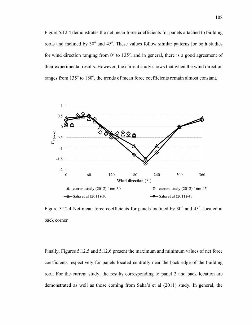
108
Figure 5.12.4 demonstrates the net mean force coefficients for panels attached to building
roofs and inclined by 30o and 45
o. These values follow similar patterns for both studies
for wind direction ranging from 0o to 135
o, and in general, there is a good agreement of
their experimental results. However, the current study shows that when the wind direction
ranges from 135o to 180
o, the trends of mean force coefficients remain almost constant.
Figure 5.12.4 Net mean force coefficients for panels inclined by 30o and 45
o, located at
back corner
Finally, Figures 5.12.5 and 5.12.6 present the maximum and minimum values of net force
coefficients respectively for panels located centrally near the back edge of the building
roof. For the current study, the results corresponding to panel 2 and back location are
demonstrated as well as those coming from Saha’s et al (2011) study. In general, the
-2
-1.5
-1
-0.5
0
0.5
1
0 60 120 180 240 300 360
CF
(m
ean
)
Wind direction ( o )
current study (2012)-16m-30 current study (2012)-16m-45
Saha et al (2011)-30 Saha et al (2011)-45

109
trends for both minimum and maximum values of the force coefficient follow the same
pattern. The small discrepancies observed between the two studies can be attributed to
different testing conditions; Saha et al (2011) conducted a wind test with suburban
exposure, while an open terrain exposure was used for the current study.
As can be observed by Figure 5.12.5, the maximum values of force coefficients
corresponding to Saha’s et al study with panel inclined by 15o are greater in total.
Moreover, Figure 5.12.6 points out that Saha’s et al (2011) experimental results show
slightly greater force coefficients in terms of absolute values compared to the values of
the current study.
Figure 5.12.5 Maximum force coefficients for panels inclined by 15o and 20
o, located at
central back position
-2
-1.5
-1
-0.5
0
0.5
1
1.5
2
0 15 30 45 60 75 90 105 120 135 150 165 180
CF
, m
ax (
net
)
Wind direction ( o )
Saha et al (2011)-15 current study (2012) - H=7m - 20 current study (2012)-H=16m - 20

110
Figure 5.12.6 Minimum force coefficients for panels inclined by 15o and 20
o, located at
central back position
-2
-1.5
-1
-0.5
0
0.5
1
1.5
2
0 15 30 45 60 75 90 105 120 135 150 165 180
CF
, min
(n
et)
Wind direction ( o )
Saha et al (2011)-15 current study (2012)- H=7m-20 current study (2012) - H=16m-20

111
CHAPTER 6: SUMMARY AND CONCLUSIONS
6.1 SUMMARY
The scope of this study was to better understand the wind pressure distribution on stand-
alone panel surfaces and panels attached to flat building roofs. For this purpose,
sophisticated physical models of solar panels of different configurations were constructed
and appropriate instrumentation was used during the experimental process in the
boundary layer wind tunnel in order to evaluate relevant wind-induced loads.
A complex model was constructed using a 1:200 geometric scale. Three model panels
were equipped with 36 pressure taps in total (both surfaces) for point and area-averaged
pressure/force measurements. Pressure and force coefficients were computed for every
pressure tap and for all the panels. Different configurations were tested under similar
conditions in order to examine the effect of each parameter on the experimental results.
6.2 CONCLUSIONS
The conclusions of this study can be summarized as follows:
The wind direction of 135o can be considered critical since most critical pressure
coefficients occur for this wind direction. More specifically, the greatest suction is
experienced by the corner panel located at the roof corner facing the wind flow
(panel 1) for 135o wind direction. The most critical values of local net pressure
coefficients occur at pressure tap denoted “1” which is found at the upper corner
of panel 1.
112
The net values of pressure coefficients corresponding to different configurations
are affected by the panel inclination for the critical 135o wind direction. For
panels located at the ground level, increasing panel inclination results in greater
suction, as well as for panels attached to 7 m and 16 m high buildings, located at
the back position of the roof. On the contrary, for front located panels attached to
7 m and 16 m high buildings, suction becomes smaller with increasing panel
inclination.
The increase of building height for panels which are located at the front position
of the building roof results in slightly smaller suction, while for panels located at
the back, the suction remains almost constant for 135o wind direction.
As far as the panel location is concerned, clearly back located panels suffer higher
suction than front located panels, at least for the critical 135o wind direction.
From all configurations examined, panel 1 shows the greatest net force coefficient
values because it is located at the roof corner and exposed obliquely to the 135o
angle of attack. The suction becomes even greater for this panel when located at
the back position of the roof.
Considering the building height, it is clear that higher suction occurs for panel 1
(corner panel), at the front location and the 135o wind direction. Middle-panel
(panel 2) follows with slightly smaller suction and finally the corner panel (panel
3) sees the smallest suction.
Comparison of the two panel locations (i.e. front and back) demonstrates that
force coefficients are greater for the back located corner panel at the roof building
when exposed obliquely to the wind. However, for the same exposure, the values

113
of force coefficients for the middle-panel (panel 2) and the other corner panel
(panel 3 is at the opposite side of the one facing the wind flow) are greater when
they are located in the front of the building.
The net values of force coefficients with respect to the wind direction show
clearly that the extreme values appear within the range of 105o and 180
o wind
directions. For all the configurations examined, the force coefficients are larger
for the corner panel (panel 1).
Comparison of the experimental results of the current study with those of previous
studies show that the values of net mean force coefficients are in good agreement,
while discrepancies are observed for the net peak force coefficient values.
6.3 RECOMMENDATIONS FOR FURTHER STUDY
The effect of a number of different parameters were examined in the current study,
however, more experimental work in the wind tunnel could offer the opportunity to
investigate the effect of additional important parameters.
One parameter related to a better performance of solar panels is the panel inclination,
which in some cases exceeds the 45o or is smaller than 20
o. Therefore, further
investigation for more panel inclinations would be necessary. Furthermore, solar panels
are often located on flat roofs in different rows of arrays and very little provision is
available for this case. It should also be mentioned that, experiments should be carried
out for different types of terrain so as to better examine the effect of landscape in the
panel wind loading.

114
Moreover, it would be really interesting to examine cases of inclined panels attached to
pitched roofs with different slopes than the roof because studies so far focus mainly on
panels located parallel to roofs. Other parameters that should be further inspected because
of their contribution in better panel functionality are the gaps between the panels and the
roof, as well as, the distance among the panels. Careful examination of these parameters
would provide information useful in determining the design wind loads in which
structures are subjected and improving the building code.

115
REFERENCES
Bienkiewicz, B., & Endo, M. (2009). Wind Considerations for Loose-Laid and
Photovoltaic Roofing Systems. Structures Congress 2009 (pp. 1-10). Austin,
Texas, United States: American Society of Civil Engineers.
Bitsuamlak, G. T., Dagnew, A., & Erwin, J. (2010). Evaluation of wind loads on solar
panel modules using CFD simulation (CWE2010). The fifth International
Symposium on Computational Wind Engineering Conference. Chapel Hill, NC.
Blackmore, P. A., & Geurts, C. P. (2008). Wind loads on roof mounted PV modules.
Paper presented at the WES Conference. Guildford, UK.
Bronkhorst, A. J., Geurts, C. P., Bentum, C. V., & Grepinet, F. (2010). Wind tunnel and
CFD modelling of wind pressures on solar energy systems on flat roofs. 5th
International Symposium on Computational Wind Engineering (CWE2010), (p.
8). Chapel Hill, North Carolina, USA.
Chung, K., Chang, K., & Chou, C.-C. (2011). Wind loads on residential and large-scale
solar collector models. Journal of Wind Engineering and Industrial
Aerodynamics, 99(1), 59 - 64.
Chung, K., Chang, K., & Liu, Y. (2008). Reduction of wind uplift of a solar collector
model. Journal of Wind Engineering and Industrial Aerodynamics, 96(8-9), 1294-
1306.

116
Chung, K.-M., Chang, K.-C., & Chou, J.-C. (2009). Wind Loading of Solar Collector
Models. The Seventh Asia-Pacific Conference on Wind Engineering, (pp. 631-
634). Taipei, Taiwan.
Geurts, C., & Steenbergen, R. (2009). Full scale measurements of wind loads on stand-
off photovoltaic systems. In C. Borri (Ed.), 5th European and African conference
on wind engineering (EACWE), (pp. 1-12). Florence, Italy.
Hosoya, N., Cermak, J. E., & Steele, C. (2001). A Wind-Tunnel Study of a Cubic
Rooftop AC Unit on a Low Building. 9th Americas Conference on Wind
Engineering (ACWE), (pp. 1-10). Clemson, South Carolina, USA.
Houghton, E. L., & Carruthers, N. B. (June 1976). Wind Forces on Buildings and
Structures: An Introduction. John Wiley & Sons Inc.
Kopp, G. A., Surry, D., & Chen, K. (2002). Wind loads on a solar array. Wind and
Structures, 5(5), 393-406.
Liu, H. (1990). Wind Engineering: A Handbook for Structural Engineers. (B. M. Stewart,
Ed.) USA: Prentice-Hall.
Meroney, R. N., & Neff, D. E. (2010). Wind effects on roof-mounted solar photovoltaic
arrays: CFD and wind-tunnel evaluation. 5th International Symposium on
Computational Wind Engineering (CWE2010), (pp. 1-8). Chapel Hill, North
Carolina, USA.
Radu, A., & Axinte, E. (1989). Wind forces on structures supporting solar collectors.
Journal of Wind Engineering and Industrial Aerodynamics, 32(1-2), 93-100.

117
Radu, A., Axinte, E., & Theohari, C. (1986). Steady wind pressures on solar collectors on
flat-roofed buildings. Journal of Wind Engineering and Industrial Aerodynamics,
23(0), 249-258.
Ruscheweyh, H., & Windhövel, R. (2011). Wind loads at solar and photovoltaic modules
for large plants. 13th International Conference on Wind Engineering (ICWE13),
(pp. 1-8). Amsterdam, The Netherlands.
Saha, P. K., Yoshida, A., & Tamura, Y. (2011). Study on wind loading on solar panel on
a flat-roof building: Effects of locations and inclination angles. 13th International
Conference on Wind Engineering (ICWE13), (pp. 1-8). Amsterdam, The
Netherlands.
Shademan, M., & Hangan, H. (2009). Wind Loading on Solar Panels at Different
Inclination Angles. 11th Americas Conference on Wind Engineering, (pp. 1-9).
San Juan, Puerto Rico.
Shademan, M., & Hangan, H. (2010). Wind loading on solar panels at different azimuthal
and inclination angles. The Fifth International Symposium on Computational
Wind Engineering (CWE2010), (pp. 1-8). Chapel Hill, North Carolina, USA.
Sparks, P. R., Akins, R. E., & Tieleman, H. W. (1981). Wind Force Coefficients for Solar
Collectors Derived from Full-Scale Load and Pressure Measurements. 4th U.S.
National Conference on Wind Engineering Research, (pp. 321-331). Seattle, WA,
USA.

118
Stathopoulos, T. (1984). Design and fabrication of a wind tunnel for building
aerodynamics. Journal of Wind Engineering and Industrial Aerodynamics, 16(2-
3), 361 - 376.
Stathopoulos, T., Zisis, I., & Xypnitou, E. (2012). Wind Loads on Solar Collectors: A
Review. ASCE/SEI Structures Congress, (pp. 1169-1179). Chicago.
Stenabaugh, S. E., Karava, P., & Kopp, G. A. (2011). Design wind loads for photovoltaic
systems on sloped roofs of residential buildings. 13th International Conference on
Wind Engineering, (pp. 1-8). Amsterdam, The Netherlands.
Wood, Graeme S; Denoon, Roy O; Kenny, C.S. Kwok;. (December 2001). Wind loads on
industrial solar panel arrays and supporting roof structure. Wind and Structures,
4(6), 481-494.
Zisis, I. (2006). Structural monitoring and wind tunnel studies of a low wooden building.
Masters thesis, Concordia University.

119
BIBLIOGRAPHY
Cook, N. J. (1985). The Designer's Guide to Wind Loading of Building Structures.
Butterworths, London: Building Research Establishment, Department of the
Environment.
Dyrbye, C., & Hansen, S. O. (1997). Wind loads on structures. John Wiley & Sons.
Lawson, T. V. (1990). Wind Effects on Buildings: Design applications. In T. V. Lawson,
Wind Effects on Buildings (Vol. 1, p. 318). Applied Science Publishers.
Simiu, E., & Scanlan, R. H. (1996). Wind Effects on Structures: Fundamentals and
Applications to Design (3rd ed.). John Wiley.

120
APPENDIX A
Appendix A includes the contour plots regarding the upper, lower surface and net values
of pressure coefficients for all configurations examined and wind direction 135o.

121
UPPER SURFACE, H = 7 m
Figure A 1 Minimum Cp values for the upper panels surface, attached to 7 m high
building and back located

122
LOWER SURFACE, H = 7 m
Figure A 2 Maximum Cp values for the lower panels surface, attached to 7 m high
building and back located

123
NET, H = 7 m
Figure A 3 Net minimum Cp values for panels attached to 7 m high building, back located

124
UPPER SURFACE, H = 16 m
Figure A 4 Minimum Cp values for the upper panels surface, attached to 16 m high
building and front located

125
LOWER SURFACE, H = 16 m
Figure A 5 Maximum Cp values for the lower panels surface, attached to 16 m high
building and front located

126
NET, H= 16 m
Figure A 6 Net minimum Cp values for panels attached to 16 m high buildings, front
located
127
UPPER SURFACE, H = 16 m
Figure A 7 Minimum Cp values for the upper panels surface, attached to 16 m high
building and back located

128
LOWER SURFACE, H= 16 m
Figure A 8 Maximum Cp values for the lower panels surface, attached to 16 m high
building and back located

129
NET, H = 16 m
Figure A 9 Net minimum Cp values for panels attached to 16 m high building, back
located

130
UPPER SURFACE, PANELS AT THE GROUND LEVEL
Figure A 10 Minimum Cp values for the upper panels surface at the ground level

131
LOWER SURFACE, PANELS AT THE GROUND LEVEL
Figure A 11 Maximum Cp values for the lower panels surface at the ground level

132
NET, PANELS AT THE GROUND LEVEL
Figure A 12 Net minimum Cp values for panels at the ground level

133
APPENDIX B
Appendix B includes the contour plots regarding the most critical values of pressure
coefficients regardless the wind direction for all configurations tested.

134
H = 7 m, FRONT LOCATION
Figure B 1 Net minimum Cp values for panels attached to 7 m high building and front
located

135
H = 16 m, FRONT LOCATION
Figure B 2 Net minimum Cp values for panels attached to 16 m high building and front
located
136
H = 7 m, BACK LOCATION
Figure B 3 Net minimum Cp values for panels attached to 7 m high building and back
located
137
H = 16 m, BACK LOCATION
Figure B 4 Net minimum Cp values for panels attached to 16 m high building and back
located

138
GROUND LEVEL
Figure B 5 Net minimum Cp values at ground level