wind farm

Valuation Models for Wind Farms under Development A Real Options Perspective

M.Sc. in Economics and Business Administration

Specialization: Finance and Strategic Management

Department of Finance

Master’s Thesis, Version 2, Incl. Appendix

Submission Date: April 8th, 2010

Supervisor: Peder Thomas Petersen

Søren Gantov Frølunde

Peter Elsborg Obling

Copenhagen Business School 2010

Executive Summary This thesis has two objectives. The first objective is to investigate the possibility of developing a

real options valuation model to improve the valuation of a wind farm under development compared

to discounted cash flow valuation models. The second objective is to compare the usability of these

models. In order to reach the two objectives we use a case study approach with a valuation of a

Danish wind farm under development. Before the valuation a thorough comparative analysis of the

different valuation models is undertaken to create a deeper understanding of the reasoning behind

them. The thesis thus has both a theoretical and practical scope; but with an emphasis on the

practical, as the discussion of theory revolves around solving practical issues.

After the introduction, the second chapter presents the case, which includes a discussion of the

process of developing wind farms in Denmark, the electricity market and the electricity price. The

chapter thereby provides some fundamental insights about wind farm development and its main

value drivers. We end this chapter with the observation that real options valuation seems suitable

for investments in wind farms under development.

The next chapter in the thesis is the theoretical discussion where the different valuation models are

evaluated on four criteria that are particularly relevant for a valuation model of wind farms under

development. In the discussion, it becomes clear that the assumptions of all financial models are

strong, and that real options valuation models should not be discarded due to this factor. Instead the

models’ ability to improve decision making in a company should be the focus and here the real

options valuation model has much to offer. Based on this potential, as well as the real options

valuation model’s superiority in handling uncertainty and flexibility, we find that it is a better model

for valuing wind farms under development than the DCF based alternatives.

In the two practical valuation chapters we develop our six step real options valuation model for

wind farms under development, by gradually increasing the amount of factors taken into

consideration. The model demonstrates the possibility of actually implementing real options

valuations in a meaningful way by practitioners, such as the case company European Energy. The

valuation does however underline the novelty of the field by highlighting the complications of

estimating volatility and including the value of the interest tax shield.

The conclusion of the thesis is that while we can develop theoretically advanced valuation models,

their practical value and usability can be debated based on the difficulties of finding reliable

estimates.

1

Table of Contents

1 Introduction ........................................................................................................... 3

1.1 Background and Objectives ................................................................................................. 3

1.2 Problem Definition ............................................................................................................... 4

1.3 Target Group ........................................................................................................................ 5

1.4 Structure ............................................................................................................................... 5

1.5 The Research Approach ....................................................................................................... 6

1.6 Delimitations ........................................................................................................................ 9

2 Wind Farm Development in Denmark ............................................................... 11

2.1 Introduction to the Case ..................................................................................................... 11

2.2 Introduction to the Danish Wind Market ........................................................................... 12

2.3 Development of a Wind Farm in Denmark ........................................................................ 13

2.4 Understanding the Tariff that Wind Farms Receive for Electricity ................................... 19

2.5 Wind Power’s Impact on the Electricity Market ............................................................... 23

2.6 Recapitulation .................................................................................................................... 24

3 Financial Theory and Valuation Models ........................................................... 26

3.1 Corporate Finance and Decision Making ........................................................................... 26

3.2 Four Evaluation Criteria for Financial Valuation Models ................................................. 27

3.3 Standard Discounted Cash Flow Model............................................................................. 29

3.4 Expected Net Present Value Model ................................................................................... 34

3.5 Decision Tree Analysis ...................................................................................................... 36

3.6 Real Options Valuation ...................................................................................................... 39

3.7 Analyzing the Estimates..................................................................................................... 54

3.8 Recapitulation .................................................................................................................... 56

2

4 Valuation of a Wind Farm under Development ................................................. 58

4.1 Introduction ........................................................................................................................ 58

4.2 DCF Value of Operational Phase ....................................................................................... 59

4.3 Expected Net Present Value ............................................................................................... 73

4.4 Binomial Real Options Valuation ...................................................................................... 76

4.5 Quadranomial Real Options Valuation .............................................................................. 91

4.6 Recapitulation .................................................................................................................... 96

5 Valuation Including the Financing Decision .................................................... 98

5.1 The Financing Decision is Important ................................................................................. 98

5.2 Models for Valuing Financial Side Effects ........................................................................ 99

5.3 Inclusion of the Interest Tax Shield in the Operational Phase ......................................... 101

5.4 Inclusion of the Interest Tax Shield in the Development Phase ...................................... 105

5.5 Recapitulation .................................................................................................................. 110

6 Conclusion & Perspectives ................................................................................ 112

6.1 A ROV Model for Wind Farms under Development ....................................................... 112

6.2 The Usability of ROV Models ......................................................................................... 113

6.3 Market Uncertainty Revisited .......................................................................................... 114

6.4 Perspectives ...................................................................................................................... 115

7 References .......................................................................................................... 117

8 Appendixes ......................................................................................................... 122

3

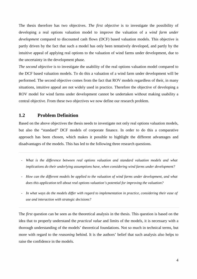
1 Introduction In this chapter we will discuss the background, motivation and target group for the thesis. This

includes a presentation of the objectives and the research question as well as a presentation of the

structure, research approach, key literature and delimitations.

1.1 Background and Objectives The production of electricity using wind energy has developed from being an enfant terrible in the

established energy industry to becoming a cornerstone in the strategy of many of the largest utilities

in Europe. The increasing interest in wind energy is based not only on the global climate debate, but

also to a large extent on issues such as energy security, the increasing demand of energy and the

sometimes high and volatile fuel costs of traditional generation technologies.

As the wind energy industry matures, investors are bound to become more professional and demand

more sophisticated analysis of investment possibilities. This demand creates a need to build a

deeper understanding of the peculiarities surrounding investments in wind farms. Before such wind

farms become operational they need to go through a highly uncertain development phase. The high

uncertainty of this development phase is partly driven by the probability of a failure during the

development phase as the wind farm can be obstructed by other stakeholders. Alternatively, the site

can turn out less attractive than first expected. Finally, the uncertainty is also driven by the

electricity price, which in several ways represents a unique commodity.

The high uncertainty is a deviation from the corporate finance literature’s standard examples, where

often very little uncertainty is present with regard to whether or not a project will be undertaken.

This is opposed to the reality in many companies, where investments are often highly uncertain. To

address these concerns real options valuation models have been suggested as a better way to include

uncertainty in investment decisions (Myers 1984a). Therefore it seems like a natural next step for

the valuation of wind farms to investigate such models as it could potentially lead to better

investment decisions. An improvement of wind farm valuations could lead to better access to

capital markets for wind farm owners, whether raising new capital or selling assets in development.

Despite the appeal of real options valuation (ROV) leading to better investment decisions, the

model is still an outsider in corporate finance. The model can therefore, just like investments in

wind farms, be seen as a relative newcomer within corporate financial analysis. This is particularly

true in the case of ROV of wind farms under development where very little research has been done.

4

The thesis therefore has two objectives. The first objective is to investigate the possibility of

developing a real options valuation model to improve the valuation of a wind farm under

development compared to discounted cash flows (DCF) based valuation models. This objective is

partly driven by the fact that such a model has only been tentatively developed, and partly by the

intuitive appeal of applying real options to the valuation of wind farms under development, due to

the uncertainty in the development phase.

The second objective is to investigate the usability of the real options valuation model compared to

the DCF based valuation models. To do this a valuation of a wind farm under development will be

performed. The second objective comes from the fact that ROV models regardless of their, in many

situations, intuitive appeal are not widely used in practice. Therefore the objective of developing a

ROV model for wind farms under development cannot be undertaken without making usability a

central objective. From these two objectives we now define our research problem.

1.2 Problem Definition Based on the above objectives the thesis needs to investigate not only real options valuation models,

but also the “standard” DCF models of corporate finance. In order to do this a comparative

approach has been chosen, which makes it possible to highlight the different advantages and

disadvantages of the models. This has led to the following three research questions.

- What is the difference between real options valuation and standard valuation models and what

implications do their underlying assumptions have, when considering wind farms under development?

- How can the different models be applied to the valuation of wind farms under development, and what

does this application tell about real options valuation’s potential for improving the valuation?

- In what ways do the models differ with regard to implementation in practice, considering their ease of

use and interaction with strategic decisions?

The first question can be seen as the theoretical analysis in the thesis. This question is based on the

idea that to properly understand the practical value and limits of the models, it is necessary with a

thorough understanding of the models’ theoretical foundations. Not so much in technical terms, but

more with regard to the reasoning behind. It is the authors’ belief that such analysis also helps to

raise the confidence in the models.

5

The second question is the practical analysis of the theories taking into consideration an actual

investment. Here the key focus is the different models’ estimation and calculation techniques as

well as the result obtained. The analysis of the practical implementation also includes a discussion

of the improvement possibilities embedded in real options valuation versus other models. Finally

the analysis highlights the more practical problems of applying abstract theoretical models to real

investment decisions. The third question will not be treated separately – instead it should be viewed as the continuous

emphasis on the practical dimension in the abstract models, as well as an explicit emphasis on the

usability dimension in the theoretical analysis.

1.3 Target Group The emphasis in this thesis on the investment decisions of wind farms under development makes it

especially interesting for active participants in such decisions. Participants include not only the

decision makers, often represented by management, but also the financial analysts who support the

decision making process, as the goal of the thesis is to contribute to the practical field of wind farm

valuations. This does not imply that the thesis is written in such a manner that any practitioner could

understand it and a certain amount of familiarity and knowledge of financial modeling is required of

the reader. Due to the necessity of investigating the assumptions and reasoning in the models (as

argued for above), the thesis is also relevant for students or other academics with a more general

interest in understanding the reasoning behind financial valuation models. This is especially true for

our own education at Copenhagen Business School in finance and strategic management, since

ROV highlights the interaction between finance and strategy.

1.4 Structure The structure of the thesis is illustrated in Figure 1.1 below. To ensure the practical dimension

throughout the thesis, it has been written as a case study for the Danish independent power producer

European Energy A/S. Hence the point of departure in the thesis is an introduction to European

Energy and one of their wind farms under development in chapter 2, along with some general

considerations about the development of wind farms in Denmark. This chapter and our theoretical

analysis in chapter 3 can be seen as the frame of reference for the actual valuations conducted in

chapter 4 and 5. We conclude the thesis with a discussion of the findings and reflections on the

6

future of real options valuation for wind farms, and the thesis ends with a more abstract perspective

of real options valuation’s relation to other fields of management studies.

Figure 1.1 Thesis Structure

Source: Own construction

1.5 The Research Approach The following is an initial clarification of our research approach, data collection and choice of

theories laid out in order to improve the arguments and choices that are made throughout the thesis.

Such a clarification can also assist a reader in understanding the arguments, interpretations and

theoretical choices throughout the thesis.

The way which we have chosen to approach the problem and structure our thesis is influenced not

only by our own assumptions, but also by the theoretical field of the thesis and its paradigm.

Financial theory has grown out of an economic science with a positivistic approach and tradition.

The economic models are based on some strong assumptions about human nature (rational) and

markets (efficient). The positivistic basis of the economic models means that they are based on

Wind Farm Development in Denmark Financial Theory and Valuation Models

Valuation of a Wind Farm Under Development

Introduction

Conclusion and Perspectives

Conclusion Perspectives

Standard DCF Expected NPV Decision Tree Analysis

Real Options Valuation

Valuation Including the Financing Decision

Background and Objectives

Problem Definition

Research Approach Delimitations

The Case Development of a Wind Farm

Wind Farm Tariff Electricity Prices

Operational Phase Expected NPV Binomial ROV Quadranomial

ROV

Frame of Reference

The Financing Decision APV vs. WACC ENPV with Debt Quadranomial

ROV with Debt

7

analytical and mathematical arguments, which can accordingly be verified by empirical studies.1

This approach can be seen in relation to the problem definition and the related requirement that the

study should be based on models, which meet such assumption and on a valid dataset.

The positivistic approach to a social science is hard to fulfill in reality as the knowledge within this

field affects the object, which is studied. This means that there is a two-way relationship between

the knowledge produced and society, known as the “double hermeneutic” (Giddens 1979: 232). An

example could be a standard net present value calculation of stock using discounted cash flows. If

this is accepted as a general model, then it is likely that we will actually influence the value of

traded stock so that our empirical data will verify our theory. Such insight highlights the fact that

empirical data is not always “pure” and models will always be abstract constructions of a complex

reality. It is to a large extent such insights that make the third question in our problem definition

necessary. The research approach in the thesis can thus be seen as on one hand being deductive

using the logic and theoretical assumption of the financial models – while at the same time

acknowledging the necessity of inductive empirical studies that seek to verify as well as critically

reflect upon the theory of the financial models. In our thesis this has been done by using the case

study approach.

1.5.1. Case Study Our case has been provided by European Energy and consists of a site with the potential to develop

a three turbine wind farm in Western Denmark. The case study approach is built on an insight that

totally predictive and universal theories of the human nature and society do not exist. Therefore

concrete, contextualized knowledge is often more valuable than universal laws and as such science

can develop itself based on “the good example” (Flyvbjerg 1991: 144). This approach does not

negate large quantitative studies, but simply points to the fact that especially in situations where

research aims at developing models, insights and “expert” knowledge – the case study is very

valuable. It is important to be careful with generalizations in case studies, however this problem

also exists for studies based on much larger (quantitative) datasets, and it actually turns out that data

found in case studies is often very valuable also for more abstract generalizations (Flyvbjerg 1991:

157). Therefore we believe that the case study as method can provide valuable insights into the

theory and use of financial valuation models for wind farms under development in line with our

three research questions.

1 Definition of positivism: a theory that theology and metaphysics are earlier imperfect modes of knowledge and that positive knowledge is based on natural phenomena and their properties and relations as verified by the empirical sciences (Merriam-Webster, 2008).

8

1.5.2. Data collection As the research questions are defined to consider theoretical issues, practical use and decision

making in companies, it has been necessary to gather data for the study. This has been done both

through primary and secondary sources. The primary data collection has been done for quantitative

and qualitative data, where the latter has been obtained through “informant interviews”. This type of

interviews is deemed particularly relevant for getting information which is hard to observe or is of a

private nature and can furthermore help to highlight the most critical issues, which need to be

further investigated (Andersen 2002: 211).

The two different types of data sources are used to heighten the validity of the arguments as we aim

to compare, critically reflect upon and use several sources for the various estimates when possible.

Such an approach thereby makes it possible to determine what “best practice” is and give concrete

recommendations based on both theoretical and empirical considerations.

1.5.3. Literature Many of the above considerations are relevant for the choice of literature as well, which we have

split in two categories: practical and theoretical literature. This distinction is somewhat artificial as

much of the literature deals with both categories but usually has an emphasis on one of them. To

create consistency between literature and research approach, it is an important criterion to consider

the coherence between the chosen theory and the approach of the thesis. The literature used in the

thesis relates to the economic paradigm, while in many cases also critically reflecting upon it and

the criterion is thus met. To avoid any theoretical or practical bias, literature has been used which is

both positive and negative towards the different models.

1.5.3.1. Theoretical Literature

The theoretical literature used in the thesis generally has its focus more on conceptual problems and

technical issues of both real options valuation and corporate finance in general. This includes texts

such as Hull (2008), Lander and Pinches (1998), Miller and Park (2002), Myers (1984a) and

Trigeorgis (1996). In addition the classic financial text book by Brealey et al. (2006) has been used;

a book which is perceived as representing what is referred to as traditional corporate finance

literature.

9

1.5.3.2. Practical Literature

The practical literature is the literature which is to a greater extent focused on providing concrete

solutions to the actual valuation practice. This literature can be split up in to two subcategories, one

containing literature which is very focused on the operationalization of models in the corporate

context and a second subcategory, which is more focused on solving specific technical issues. The

first is represented by authors such Copeland and Antikarov (2003), Mun (2006), Shockley (2007)

Villiger and Bogdan (2005a), Willigers and Hansen (2008). It is such literature which is referred to

as the practical real options literature in the thesis. Much of this literature is however interested in

promoting real options valuation and therefore literature with a more critical approach has been

taken into considerations as well, to balance the arguments.

The second subcategory of practical literature is not used in the same way throughout the thesis.

Instead we have used it to get ideas of how to perform concrete estimations. This subcategory

includes literature such as Bøckman et al. (2007) but also “classics” like Brealey et al (2006) and

Koller et al. (2005).

1.6 Delimitations The scope of the thesis is quite broad since several different models are compared on different

levels. Given the complexity of the real options models, it is necessary to limit the amount of topics

which are treated thoroughly in the thesis.

1.6.1. Wind Farms under Development Any investment is subject to a large amount of uncertainties, random events and possible strategies.

To narrow the focus of the thesis, especially considering the uncertainty and event estimates, the

thesis is focused on a wind farm under development and the probability of it actually being

constructed.

1.6.2. Traditional Valuation Models Out of the many financial valuation models used in corporate finance, we have chosen the standard

DCF model, Expected Net Present Value Model and Decision Tree Analysis as the traditional

models to compare real options valuation with. This is done based on the notion that the DCF based

models currently represent the standard valuation model (Copeland and Antikarov 2003: V) and

that these models are the ones which real options valuation is generally compared to in the

literature.

10

1.6.3. Real Options Valuation Models The options’ field has produced a tremendous amount of literature since the breakthrough of Black,

Scholes and Merton in 1973. We have chosen to focus on the binomial model, as this is the model

generally suggested by the practical real options literature to be best suited for valuing real

investments. The choice of this model is in line with an outspoken desire among practitioners that

real options literature should focus more on practical applications than model fine tuning (Miller

and Park 2002: 129).

1.6.4. Theoretical Focus The theoretical focus of the thesis is on the reasoning process of the models more than the

mathematical or technical issues of the models. These issues are therefore only discussed when the

authors deem that they add value to the reasoning behind the model. This is based on an idea that

the introduction of complex mathematics would have changed the character of the thesis, giving

less space to the issues which are crucial for decision making, and made it less approachable from

the viewpoint of a non-financial or non-technical decision maker.

1.6.5. Estimates In the assessment of technical issues regarding the development of wind farms such as wind

characteristics and production data for wind farms, we have used the estimates provided by our

external sources, since these issues are outside our area of expertise. The assessment of the

development probabilities has also been done by the experts who are actually working in the

industry, as we have very little chance of estimating such probabilities. We have as authors however

influenced the estimates, in the sense that we have based our estimates on the opinion of several

developers and as such have been responsible for synthesizing the information of the different

sources.

1.6.6. Time Frame Based on the fact that the writing of a thesis and construction of a valuation is a-work-in-progress

until it is submitted, it is necessary to define a time frame to avoid changing estimates and refining

the arguments for eternity. Thus we have chosen the 31th of December 2009 as a cut-off date, and

have only considered data available prior to this date.

11

2 Wind Farm Development in Denmark In the following chapter the case, a Danish wind farm under development, is introduced.

Furthermore the chapter has two main objectives. The first is to give an understanding of the

development process of a wind farm in Denmark. The second objective is to introduce the electricity

market and the price dynamics of electricity. The information about the case, the development

process, and the electricity price provided in this chapter, is the basis for the valuation conducted

in chapter 4.

2.1 Introduction to the Case European Energy (EE) has recently decided to start developing wind farms in Denmark. EE has

now located several attractive sites, and needs to decide which ones to develop. To make this

decision, they need to estimate the value of their different sites.2

To develop a model which is able estimate this value, we have chosen a case study approach. We

will use the following case to test various valuation models. The case should not be perceived as

one specific wind farm with focus on the circumstances for a particular location, but as an average

wind farm under development. Thus many of the estimates in the practical valuation will be average

estimates from various professional developers. The idea is that EE or other developers can change

the variables in our model according to a specific wind farm, but use our estimates as benchmarks.

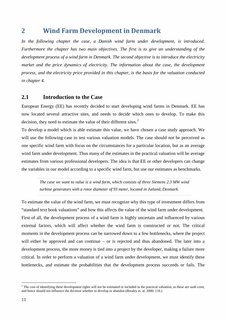
The case we want to value is a wind farm, which consists of three Siemens 2.3 MW wind

turbine generators with a rotor diameter of 93 meter, located in Jutland, Denmark.

To estimate the value of the wind farm, we must recognize why this type of investment differs from

“standard text book valuations” and how this affects the value of the wind farm under development.

First of all, the development process of a wind farm is highly uncertain and influenced by various

external factors, which will affect whether the wind farm is constructed or not. The critical

moments in the development process can be narrowed down to a few bottlenecks, where the project

will either be approved and can continue – or is rejected and thus abandoned. The later into a

development process, the more money is tied into a project by the developer, making a failure more

critical. In order to perform a valuation of a wind farm under development, we must identify these

bottlenecks, and estimate the probabilities that the development process succeeds or fails. The

2 The cost of identifying these development rights will not be estimated or included in the practical valuation, as these are sunk costs, and hence should not influence the decision whether to develop or abandon (Brealey et. al. 2006: 116.)

12

identification of these development stages and estimation of their success probabilities is one of the

two main objectives in this chapter.

Besides the risk of failing under development, the value of a wind farm under development is

highly dependent on the value of the wind farm once it becomes operational. An operational wind

farm receives a tariff, combined of a subsidy and the market price for electricity. Thus the value of a

wind farm under development is highly correlated with the electricity price, and a decreasing

electricity price could result in an unprofitable project and lead the developer to abandon a wind

farm under development. The second objective of this case chapter is therefore to develop an

understanding of the very volatile commodity electricity, as this knowledge is fundamental in the

estimation of the expected value of the wind farm. Before discussing these two objectives, we will

give a short introduction to the Danish wind market and the case company European Energy.

2.2 Introduction to the Danish Wind Market Since modern wind farm development started in Denmark more than 30 years ago, Denmark has

developed into one of the leading countries in the world in terms of installed wind power capacity,

with more than 3,406 MW covering almost 20% of the national electricity demand (Emerging

Energy Research 2009a: 11). Despite this impressive history, the installed capacity has nearly

stagnated since 2003. This stagnation has primarily been caused by political reasons. But in

December 2008 the political climate has changed once again with the introduction of the VE-Law, a

new law which is meant to facilitate wind farm development in Denmark.3 This law contains a

number of initiatives to incentivize investments in wind energy, such as requiring that individual

municipalities locate designated wind turbine areas, a “smoother” administration, initiatives to

address neighbors and other stakeholders and finally a new subsidy system once again attracting

investors to develop wind farms in Denmark. These investors are different from previously.

Traditionally, wind farms in Denmark have been developed and owned by small scale private

investors. But as wind farm investments have developed throughout Europe, the industry has

attracted more professional investors such as EE, who have the resources to develop projects in a

larger scale.

2.2.1. European Energy – an Independent Power Producer from Denmark European Energy is an independent power producer (IPP) within the renewable energy industry,

focused on developing new projects and holding and selling of electricity to the local grid. The

3 Law nr. 1392 af 27/12/2008, ”Lov om fremme af vedvarende energi”.

13

company is privately owned by the management, and was founded in 2004. Since then, EE has

grown rapidly and is today one of the largest independent power producers (IPP) in Denmark. Until

now, EE has focused on the development in other European countries. But with the introduction of

the new VE-law, EE now sees Denmark as a good business opportunity where they can combine

their experience from abroad with their local knowledge.

EE consists of almost 200 smaller companies, but overall it is divided into the mother company

European Energy A/S, and the three daughter companies European Solar Farms, A/S, European

Wind Farms A/S and European Hydro Plants A/S. The three daughter companies each contain a

number of smaller companies or so-called Special Purpose Vehicles (SPV) within respectively

hydro, wind and solar projects. Each SPV is a legal entity – so a bankruptcy of one will not

influence the other SPVs. Furthermore it gives the holding company a limited liability, so that its

maximum risk is the equity held in each SPV. This structure makes project financing possible.

This thesis is written in close collaboration with EE as they have provided the case for the

valuation. Hence the analysis is seen from their perspective, why they will be mentioned throughout

the thesis. But as the purpose of this thesis is to develop a more general valuation methodology, any

idiosyncratic characteristics related to EE will be explicitly stated so another developer can insert

own estimates.

2.3 Development of a Wind Farm in Denmark Based on this brief introduction to the case and the Danish wind market, we are now ready to focus

on the first of the two main objectives of this chapter, namely, to identify the stages of the wind farm

development process and to determine the cost and probabilities of succeeding in each stage. We

start by introducing the three phases of a wind farm life cycle.

2.3.1. The Three Phases of a Wind Farm Life Cycle The life cycle of a wind farm can generally be divided into three phases, a pre-development phase,

a development phase and an operational phase, which are illustrated in Figure 2.1.

14

Figure 2.1 Illustration of the Three Phases in a Wind Farm Life Cycle


In the pre-development phase, attractive locations are identified and the phase ends with a contract,

which is an exclusive agreement between the developer and land owner to develop the site. Until

the contract has been signed, the project is not regarded to be under development, and thus beyond

the scope of the thesis. With this agreement, the project enters the development phase, which is the

main focus of this thesis. This phase is highly uncertain, and the project faces a large probability of

failing in this phase due to external factors, meaning that the investor would lose the time and

money he has put into the project.

Once the project is developed and connected to the grid, it enters the operational phase. The

operational phase of a wind farm is typically expected to be 20-25 years. As we want to value a

wind farm under development, we will now analyze the 3 year long development phase further.

2.3.2. The Four Stages of the Development Phase The development phase can vary significantly between different countries, but generally it includes

some sort of feasibility study of the potential wind resources and a process of obtaining the

necessary agreements and permits before the actual construction takes place.

In Denmark the development phase can be divided into 4 stages as shown in Figure 2.1 above,

which are feasibility studies and pre-approval, VVM4 and final approval, complaints and

compensation and finally construction. As we move to the right in the figure along the 4 stages, the

project’s likelihood of being constructed will increase. The four stages of the development phase

are described in the following subsections.

4 VVM: ”Vurdering af virkning på miljøet” in English: ”Evaluation of Environmental Impact”.

Stage 1 Feasibility Studies and Pre-approval

Stage 2 VVM and Final

Approval

Stage 3 Complaints and Compensation

Stage 4Construction

Development Phase

Pre-developmentPhase

Unknown

Operational Phase

Approx. 20 Years

Development Phase

Approx. 3 Years

15

2.3.2.1. Stage 1, Feasibility Studies and Pre-approval

This stage combines two elements. First and foremost a feasibility analysis of a site and the wind

resources must be conducted. In most countries this is a time consuming and expensive stage, but in

Denmark, due to the uniform wind pattern and the experience with wind turbines, this is less

complicated (Dunlop 2004: 92). Instead, the wind resources are simulated using the software

WindPRO by EMD. The results are very predictable, and only rarely differs significantly from an

experienced developers expectations.

With the feasibility studies in place, the developer will conduct additional preliminary studies such

as noise analysis and grid connection possibilities, and ensure that the project complies with the

local area plan. When the preliminary studies are completed, an application is made to the

municipality. The application is processed in the economic and environmental committee, before

the project has a four week public hearing period. Based on these outcomes, the city council makes

a final decision to give a pre-approval or not.

2.3.2.2. Stage 2, VVM and Final Approval

If the pre-approval is granted, a more thorough environmental investigation is undertaken: the

VVM-report4. With the VVM-report in place, the official application is made. The processing of

this application includes a thorough investigation of the VVM-report by the municipality and an

eight week public hearing period. At the end of the stage, the city council gives a final permit,

leaving the actual building permit as a pure formality.5

2.3.2.3. Stage 3, Complaints and Compensation

Two types of complaints have deadlines along with the public hearing, but are treated afterwards.

The first is technical complaints regarding the VVM-report and the second is neighbors who require

compensation, due to losses in property value as a consequence of the wind farm construction. The

technical complaints are processed by Naturklagenævnet. A decision in favor of a complaint could

stop the entire project, but this is not very likely to occur.6

The second type of complaint that is treated after the public hearing, are any complaints about loss

in property value for neighbors to a wind farm. The possibility to claim compensation was

introduced as a part of the VE-law, and is named “værditabsordningen”.7 This is a new law and

only very few cases have been settled. The 1st case was settled in October 2009 with compensation

5 Interview with resigning Mayor of Ringkøbing-Skjern Municipality Torben Nørregaard, at “Dansk Vindmølle Træf 2009”, 7th November 2009. 6 Telephone interview with Susanne Spangsberg Christensen from “Naturklagenævnet”. One example of a case, where the complaints were approved, is two WTG’s in Kundby 17th June 2009. 7 Chapter 2, §6-§12, law nr. 1392 af 27/12/2008, ”Lov om fremme af vedvarende energi”.

16

to several neighbors of the wind farm Svoldrup Kær in Aars, in a range from 75.000-200.000

DKK.8 Depending on the amounts of settlements, the wind farm might simply not be profitable due

to compensations and will therefore fail.9 Furthermore the complaints entail a large cost for the

developer, since he has to spend time and money on visiting neighbors and on measuring the impact

of the wind turbine generators (WTGs).

2.3.2.4. Stage 4, Construction

The fourth and last stage of development phase is construction of the wind farm. The cost of this

stage consists of the WTG price and the cost of the installation and connection to the grid. The price

of the turbine is known in advance, whereas the construction costs might vary slightly according to

the particular site. As soon the turbine is installed and commissioned it enters the operational phase.

2.3.3. Probability and Cost Estimates for a Wind Farm under Development With the four stages identified above, we will now estimate the cost and probability of success for

each stage. As the VE-law is relatively new, and only a few projects have been developed during

this legislation, applying statistics from developed projects would not make sense. Instead we use

cost and probability estimations available from our interviews with two of Denmark’s largest

developers – Vattenfall and DONG Energy – and EE (see Appendix 4). As our purpose is to

develop a general valuation model, the interviewed developers were asked for estimations on an

average onshore wind farm. The only price that is specific for this exact case is the construction

costs of DKK 58 mil, provided by EE from an actual offer on the construction of three 2.3 MW

Siemens turbines to be constructed in year 2010. Since the turbine will not be purchased and

constructed before 2.5 years into the development phase, the cost has been adjusted for an expected

inflation of 2%, thus the construction cost are estimated to be 61 mil.10 An overview of the cost and

probabilities in the development phase can be seen from Figure 2.2 below.

8 Vindmøller og Vindenergi på land, 1. Oktober. J.nr..013848-0091 jla/jhp/ppe 9 “Cikulær nr. 9295 af 22/05/2009, Cirkulære om planlægning for og landzonetilladelse til opstilling af vindmøller”. In November 2009, Energinet.dk, which processes these complaints, had four open cases with a total of 102 claims of compensation due to value loss (Henrik Kamp, Energinet). 10 The exact amount is 60.944 mil, however we have rounded this to the nearest million.

17

Figure 2.2 Development Probabilities and Cost Estimates of Wind Farm Development

Source: Own construction, based on interviews with Danish wind farm developers (Appendix 4).

These estimates are fundamental for the practical valuation in chapter 4. As can be seen from the

figures above, the probabilities of succeeding in the first two stages are relatively low, making the

investment risky. However, the costs of the first three stages are relatively low compared to the

construction stage; hence the large cost of the turbine construction can actually be avoided if the

project fails before the final stage.

It should be noted that the cost estimation in stage 3 does not include the actual compensations, but

only the cost of undertaking the analysis, based on complaints from neighbors to find out whether

or not they are entitled to any compensation. The project is, however, modeled with the assumption

that no compensation occurs. This is based on an idea that the amount is so individual that it cannot

be included in generic statistics, using the model for a specific project. The expected compensation

could be added to the current amount of DKK 500,000.

2.3.3.1. Assumptions for Applying Probabilities

Using standardized development stages and uniform success probabilities is a strong assumption,

and we are aware that these estimations will vary between the individual projects in Denmark.

However to assign probabilities to development stages is a methodology that can be found in other

Stage 1 Feasibility Studies and

Pre-approval

Stage 2 VVM and Final Approval


Stage 4Construction

Duration of Stage

Reason for Failure

6 Months 12 months

Cost of Stage

Prob. of proceeding to next stage

100,000 DKK 500,000 DKK 500,000 DKK 61,000,000 DKK

50% 50% 80% 100%

6 Months12 months

Activities •Simulate feasibility WindPRO•Make additional preliminary studies•Apply for pre-approval

•Not Feasible•Preapproval not granted

•Perform VVM analysis• Apply for final approval

•VVM fails •Approval not granted

•Compensation makes the project unattractive•VVM approval withdrawn due to complaints

N/A

•Treat complaints and develop solutions•Negotiate fair compensations with neighbors

•Build necessary infrastructure•Build gridconnection•Install WTG

Probability of construction 20% 40% 100%80%

18

valuations, such as HSBC’s report about the world’s largest wind farm owner Iberdrola Renovables

(2008).11 HSBC furthermore use probabilities estimated by the developer Iberdrola themselves, as

they believe that “no one knows the projects better than the developers” – which can be said to be

the same case in our estimation, where we have interviewed leading developers in Denmark to

estimate these probabilities.

In the HSBC report (2008: 58-60), Iberdrola estimates the probabilities of success for “probable

projects” (more or less equal to stage 1 in our terminology) to be 20% equal to the probability of

construction in our stage 1. Their second category is “likely projects”, which is quite similar to our

stage 2, with an estimate of a 45% chance of being constructed, compared to 40% in our case. The

final category is “highly confident projects” with a success rate of 95%. This represents a project

just about to go into construction. Iberdrola’s estimates are based on other markets than the Danish

market, and cannot be used to verify our estimates. However their methodology shows us three

things. First, it demonstrates, that our estimates seem reasonable and as such provide some validity.

Secondly, it highlights the value of the knowledge from experienced developers. Thirdly, it displays

that probabilities for a wind farm under development are estimated, which might not be totally

exact, but these estimates are used in practice by investment professionals to improve valuations.

Thus we find it appropriate to use expert based probabilities in our valuation.

A second assumption of our approach is that information about development success arrives in a

non-continuous way at the end of each stage. It would be more realistic to assume a continuous

information flow within each stage. Although models could be developed with a lower detail level

and more stages, it is doubtful whether they would lead to a higher precision, due to increased

complexity and difficulties of obtaining realistic estimates (Willigers and Hansen 2008: 532).

We have now identified the 4 stages of a wind farm development, and have estimated their costs

and probabilities of success, and we continue with the second objective of the chapter – a discussion

of the electricity price.

11 Iberdrola’s figures are for their global portfolio (approx 40 GW) of projects (USA, UK, Spain and Rest of World). It is likely to assume that the figures from both our developers and Iberdrola are somewhat biased, as they are probably too optimistic concerning development. We have therefore in our estimates in general chosen the more conservative figure.

19

2.4 Understanding the Tariff that Wind Farms Receive for Electricity The following section will discuss the tariff that wind farms receive for electricity in Denmark. As a

large part of the tariff is the market price for electricity, the section will give a thorough

introduction to the unique commodity electricity. Furthermore electricity derivatives are discussed,

as these will be an important part of the valuation later in the thesis.

2.4.1. Introduction When a wind farm produces electricity and sells it to the market, it receives a price per kWh sold,

called the tariff. As wind power cannot compete with conventional electricity sources, many

countries provide attractive subsidiaries to incentivize investors to construct wind farms (dkvind

2009a: 1-3).12 In Denmark a new tariff system was recently introduced as a part of the previously

mentioned VE-law. The tariff consists of two parts; the market price for electricity plus a fixed

subsidy premium of 25 øre/kWh for the first 22.000 full load hours, which is approximately the first

10 years production (dkvind 2009a: 1).13 This is illustrated in Figure 2.3 below.

Figure 2.3 Tariff to Wind Farms in Denmark


To avoid any confusion, we will through-out the thesis use the terms from the figure when referring

to the compensation for electricity. The market price is thus the so-called spot price that is received

from sales to the electricity market, the subsidy premium is the fixed subsidy received per kWh

produced and the tariff is the total compensation received for a kWh at a given point in time.

2.4.2. Understanding the Market Price The market price or the spot price is the hourly price for electricity traded on the market. As

electricity cannot be stored efficiently, it must be used instantly after production, which makes the

spot price very sensitive to shifts in the consumer demand and the supply of electricity (Oum and 12 dkvind is the Danish Wind Turbine Owners’ Association. 13 A full load hour is defined as a turbine producing its name plate capacity i.e. 2 MWh delivered from a 2 MW turbine.

Market PriceThroughout Operational Phase

Subsidy PremiumProduction < 22,000 Full Load Hours≈ First 10 Years of Production

Tarif

f

Year 0 Year 10 Year 20

Tariff to Wind Farms in Operational Phase

20

Oren 2005: 2-3). The non-storability of electricity makes it so volatile, that electricity delivered at

two different times should be perceived as two distinct commodities, as the price can vary

considerably even within a short time interval, as seen in Figure 2.4. (Lucia and Schwartz 2002: 6).

Figure 2.4 Weekly Distribution Pattern for Spot Price (System Price), Year 2000-2008


The figure shows that the electricity price varies throughout a normal week, being lower in the

weekends than during the week and has a daily profile, where the price is significantly higher

throughout the day than during the night. Besides these daily and weekly fluctuations, it is also

affected by monthly seasonality (IBT Wind 2006: 14-16).

2.4.3. The Nordic Electricity Market The Danish electricity market and other countries have relatively recently undergone a liberalization

(Lucia and Schwartz 2002: 7). In July 1999, Denmark entered the Nordic electricity market, Nord

Pool, which is probably the world’s most well functioning electricity market (Fusaro 2004: 1). The

Nord Pool market consists of Denmark, Sweden, Norway and Finland. The benefits from an

international electricity market is a larger flexibility in the grid and ability to distribute electricity

generated from natural resources to a larger market, when it is in excess. Nord Pool does not consist

of one big market, but 8 individual markets, which is caused primarily by two factors. First,

electricity suffers from relatively expensive transmission costs due to transportation losses. Second,

a limited grid connection between the markets prevents the free movement of electricity. Because of

these limiting factors, the market conditions can vary from one market to the other, causing very

different prices on each market. Thus each market has its own price for electricity. As a common

reference point between the 8 individual markets, the so-called system price is used. This is an

arithmetic average of the 8 markets spot prices and thus reflects the overall market condition of the

Nord Pool markets (Lucia and Schwartz 2002: 7).

0

50

100

150

200

250

300

350

400

Monday Tuesday Wednesday Thursday Friday Saturday Sunday

DKK/

MW

h

Spot Price

Monday Tuesday Wednesday Thursday Friday Saturday Sunday

21

2.4.3.1. Danish Electricity Market

The Danish electricity market is split in two: DK West/DK1 consisting of Jutland and Funen, and

DK East/DK2 consisting primarily of Zealand. The markets are two separate entities, as there is no

direct connection between the two. This creates significant price differences between the two

markets, partly due to DK West having substantially more WTGs installed than DK East (IBT Wind

2006: 9). However, a connection between the two markets is currently under construction, and is

expected to be finished in late 2010 (Energinet.dk, link 1).

Denmark’s location between Norway and Sweden with cheap hydro power and the large thermal-

capacity in Germany has a huge impact on the spot price in Denmark, as Denmark serves as a

“buffer” between the two. When electricity is expensive in Germany, then Denmark imports

electricity from the Nordic neighbors and exports it to Germany and vice versa (IBT Wind 2006: 9).

The average price level of the neighboring markets can be seen from Figure 2.5, where the Danish

electricity price during the last two years has been above its Nordic neighbors, and below the

German electricity price.

Figure 2.5 Comparison of Average Electricity Prices, 2007-2008


2.4.3.2. Nord Pool Spot – The Physical Electricity Market

Nord Pool is furthermore divided into two departments, a physical market where actual electricity is

traded called Nord Pool Spot and a financial energy market Nord Pool ASA. Nord Pool Spot is an

electricity exchange owned by the member countries’ transmission system operators.14 Nord Pool

Spot is a day-ahead exchange, where electricity prices are determined for the next day. This is done

in a so-called double auction – where buyers and sellers of electricity place their bids and asks for

electricity on an hourly basis for the following day, and based on these a price is set. (Houmøller

2003: 4). As the exact consumption and production can be hard to predict with precision a day

ahead, Nord Pool also consists of an intraday market, the Elbas Market, which trades electricity up

to one hour before delivery.

14 Svenska Kraftnät, Statnett, Fingrid and Energinet.

0

100

200

300

400

Germany DK East DK West Sweden Norway

DKK/

MW

h

22

System Price Forward

CfD ForwardForward DK West

2.4.3.3. Nord Pool ASA – The Financial Electricity Market

The second part of Nord Pool is Nord Pool ASA, which is the financial market on Nord Pool. Here

energy derivative contracts are traded, creating risk management opportunities for the companies on

the market. In this section, we will focus on some of the financial electricity derivatives, because

these will be used later in the valuation.

One of the most traded derivative contracts on Nord Pool ASA are forwards on electricity. A

forward is the obligation to deliver a product at a pre-specified price and future date (Hull 2008:

781). As Nord Pool ASA is solely a financial market, no actual electricity transfer occurs; instead

the difference in price is settled through North Pool Clearing ASA (Houmøller 2009: 25). The

forwards traded at Nord Pool are either base-load or peak-load contracts, referring to the time of the

day the electricity is delivered. We will solely focus on forwards for base-load contracts. A long

position in a base-load forward, is the obligation to deliver 1 MW capacity throughout the delivery

period at a fixed price.15 The forwards on Nord Pool have delivery periods ranging from one month

up to one year. The trading period of a forward stops immediately before entering the delivery

period and is settled immediately after the delivery period. The delivery price is calculated as an

arithmetic average of the price over the delivery period.

As a forward costs nothing to hold, and is an obligation to deliver or purchase electricity on a future

date to a pre-specified price, this price must reflect the markets present expectations about the

electricity price throughout the delivery period (Black 1975: 173). If this was not the case, arbitrage

possibilities would exist on the market.

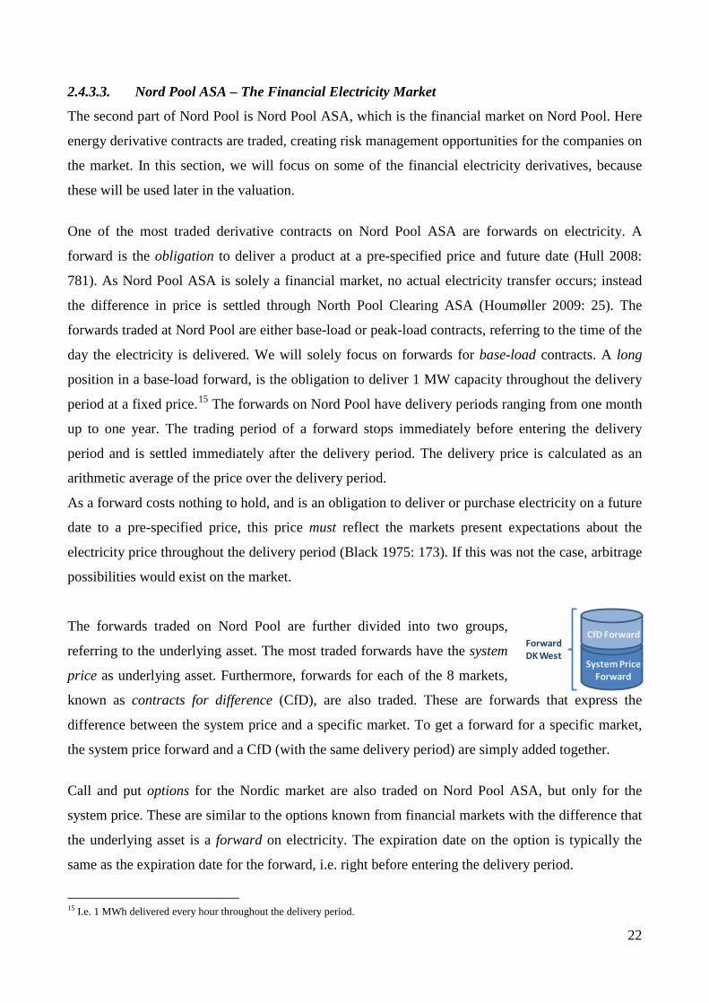
The forwards traded on Nord Pool are further divided into two groups,

referring to the underlying asset. The most traded forwards have the system

price as underlying asset. Furthermore, forwards for each of the 8 markets,

known as contracts for difference (CfD), are also traded. These are forwards that express the

difference between the system price and a specific market. To get a forward for a specific market,

the system price forward and a CfD (with the same delivery period) are simply added together.

Call and put options for the Nordic market are also traded on Nord Pool ASA, but only for the

system price. These are similar to the options known from financial markets with the difference that

the underlying asset is a forward on electricity. The expiration date on the option is typically the

same as the expiration date for the forward, i.e. right before entering the delivery period.

15 I.e. 1 MWh delivered every hour throughout the delivery period.

23

2.5 Wind Power’s Impact on the Electricity Market As previously mentioned, approximately 20% of Denmark’s total supply of electricity is delivered

from WTGs. Unfortunately this is not a stable flow of electricity, as it depends on the varying wind

resources. This has an influence on the electricity sold on the Nord Pool Spot Market, as the supply

is given a day-ahead. For wind power, this is done by the “responsibles for the balancing” (de

balanceansvarlige). As these typically administrate large portfolios of WTGs, a certain

diversification effect occurs, which enables them to give a relatively accurate estimate of the exact

production that their total portfolio of WTGs will generate on a day-ahead basis. However as the

exact production cannot be forecasted with precision, due to the fluctuating wind resources, a

deviation between the day-ahead bid and actual production will occur, which leads to a small fine.

This fine is called the balancing-cost (IBT Wind 2006: 7-8).16 To compensate for this loss, WTG

owners are subsidized with a further 2.3 øre/kWh produced (dkvind 2009a: 2). As this subsidy is

given to cover the loss from selling electricity on market terms, the subsidy will be assumed to

cover the loss exactly hence both will be disregarded for the rest of the thesis.

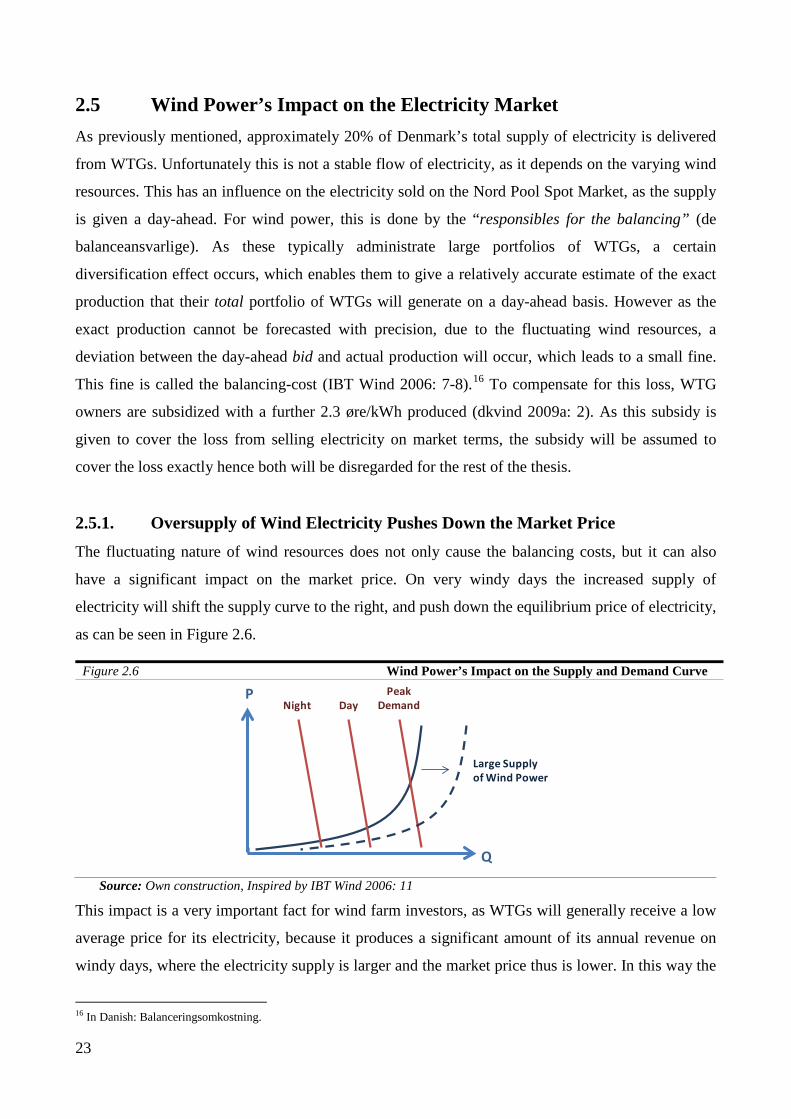
2.5.1. Oversupply of Wind Electricity Pushes Down the Market Price The fluctuating nature of wind resources does not only cause the balancing costs, but it can also

have a significant impact on the market price. On very windy days the increased supply of

electricity will shift the supply curve to the right, and push down the equilibrium price of electricity,

as can be seen in Figure 2.6.

Figure 2.6 Wind Power’s Impact on the Supply and Demand Curve

Source: Own construction, Inspired by IBT Wind 2006: 11

This impact is a very important fact for wind farm investors, as WTGs will generally receive a low

average price for its electricity, because it produces a significant amount of its annual revenue on

windy days, where the electricity supply is larger and the market price thus is lower. In this way the

16 In Danish: Balanceringsomkostning.

Q

PNight Day

Large Supply of Wind Power

Peak Demand

24

WTGs can be said to have a “cannibalizing” effect, which will increase as more WTGs are installed

in Denmark in the future. This cannibalizing effect will be referred to as the down lift.

For short periods of time, the supply from wind power can push down the prices to 0. But as

electricity has to be used and will infer a cost for the transmission system operator if in excess,

negative prices were introduced the 30th November 2009 (Energinet.dk, link 2). Negative prices

mean that when the supply is sufficiently large, the market is willing to pay for the consumption of

electricity. In the short run, this has a relatively small impact on the individual wind farm, as the

spot price has only been zero for approximately 200 hours since 2003 and new technologies are

invented, so that WTGs disconnect as the prices hits zero (Børsen, 29-10-2009). But in the long run,

as the number of installed wind capacity in Denmark increases, a price below zero could occur

more frequently. These negative prices could look like as a potential hazard for wind farm owners

but could actually end up being an advantage. Negative prices might be caused by the WTGs, but it

affects all power producers delivering to the market. The power plants that generate power from

fossil fuels could thus end with a higher marginal cost from continuing their production, as

compared to shutting down. Negative prices could thus act as an incentive for these power plants to

use electricity for heating or storage, when prices are sufficiently low (dkvind 2009a: 3). Other

initiatives, such as the cable between DK West and DK East, are also expected to stabilize the

prices in windy periods further because this opens up for the possibility of selling the excess supply

to other markets.17 The discussion of price patterns will be continued in the practical valuation.

2.6 Recapitulation We started this chapter by presenting the investment opportunity to develop a 3 WTG wind farm in

Jutland, which the case company European Energy identified. To make an investment decision

about this site, EE is interested in developing a valuation model, which is able to estimate the value

of this wind farm under development.

To perform the valuation, it is necessary to understand the life cycle of a wind farm in general and

more importantly the development phase. In the chapter we identified 3 phases in the wind farm life

cycle and 4 stages in the development phase, as seen in Figure 2.1. The development phase is costly

and outside events could induce it to fail, therefore such events should be included in the valuation.

As a result, we assigned a success probability and a cost for each stage of the development phase.

Furthermore we discussed that wind farms in Denmark are very sensitive to the electricity price, as

17 However the cable is only 600MW, so low and negative prices are still expected to occur (Dorthe Vinther, Energinet).

25

a large part of the tariff they receive depends on this price. Since these electricity prices are very

volatile, a wind farm is subject to a substantial amount of uncertainty during the development

phase, because a decline in the price could make the development of the wind farm unattractive.

These two characteristics of a wind farm under development: that it is a staged investment process,

and it is subject to a large degree of uncertainty suggests that such an investment is particularly

suitable for a real options valuation, as we discuss in the following chapter.

26

3 Financial Theory and Valuation Models In this chapter we introduce the financial models for valuing a wind farm under development. The

chapter starts by setting up four important criteria that the valuation models are evaluated upon.

These criteria are used for a more extensive comparison of the different models consisting of the

standard discounted cash flow model, the expected net present value model, decision tree analysis

and real options valuation.

3.1 Corporate Finance and Decision Making The purpose of corporate finance is in essence to maximize the wealth of shareholders by applying

the market value maximization principle, such that a corporation should only invest in a project that

increases the market value of the firm represented by a positive NPV (Arnold and Shockley 2003:

82). 18 To achieve the goal of value maximization, corporate finance supports two decisions. First, it

determines the optimal investment decision – or what investments a company should undertake, and

second, the optimal finance decision – or how the investment should be paid for. Corporate finance

decisions are thus closely related to the strategic decisions through the influence on the allocation of

capital and funding of projects. Despite this close relation, traditional valuation models, based on

discounted cash flows, are not good at incorporating decisions into the value of an investment.

These models have therefore been criticized for lacking ability to reflect the actual value of an

investment decision and as a tool for strategic decision making (Myers 1984a: 127). In our case, the

valuation of a wind farm under development, this is problematic because EE is able to make

decisions during the development phase.

EE could therefore benefit from a valuation model which is able to include the value of decision

making during the development phase. This has, more generally, been formulated by Myers (1984a)

as the need for developing a model that bridges the gap between strategic decision making and

finance, or more realistically brings the two closer to each other. To bridge the gap, Myers (1984a:

136) suggests two solutions: to improve the application of existing valuation models and to look at

the possibility of including option pricing techniques.19 This chapter therefore has two purposes:

First, it will be an analysis of traditional valuation models in comparison to real options valuation.

18 Brealey et al., (2006: 25-29) point out that it is not given that all corporations will follow this criteria and many corporations might consider wealth maximization more broadly than just value for shareholders. Although this seems reasonable, standard corporate finance theory uses the NPV as the decision criterion when discussing different theories and investment opportunities including Brealey et al. themselves. 19 By existing theory Myers (1984a) is referring to standard DCF based valuation techniques.

27

This leads to the second purpose, which is to improve our understanding of how these models can

be used for the valuation of wind farms under development.

3.2 Four Evaluation Criteria for Financial Valuation Models Before starting the examination of the valuation models, we set up four criteria to evaluate the

valuation models upon, which can be seen in Table 3.1. These criteria are chosen to deepen the

understanding of the assumptions and limitations of the different models as well as their usability in

practice. The four criteria touch upon what Plenborg (2000: 2-3) calls the fundamental requirements

of the model and the cosmetic requirements. The fundamental requirements address the realism of

the models’ assumptions and whether they give a precise (unbiased) result, whereas the cosmetic

requirements focus on user-friendliness and intuition of results. The fundamental requirements

dominate the cosmetic ones, as deviations from the prior can lead to irrational investment behavior.

However, the importance of cosmetic requirements should not be underestimated, as it is of great

importance for management to be able to understand the model – and as such important for bridging

the gap between strategy and finance. It is therefore important to address both requirements, when

setting up criteria for evaluating valuation models. Throughout the chapter, the four criteria are

discussed, one by one and applied to each model, each time focusing on the two sub-criteria.

Table 3.1 Four Evaluation Criteria for Financial Valuation Models

Fundamentals Flexibility

Object of Analysis Modeling Event Decision

Market Uncertainty Usability

Perception Measure Implementation Interpretation

Source: Own construction inspired by Dam-Rasmussen and Würtz (2003), Plenborg (2000) and Skjødt (2001).

Fundamentals

This fundamental criterion is intended to build up an understanding and provide the background of

the models. It pertains to a discussion about the models’ origin, object of analysis and their way of

modeling in time.

Market Uncertainty

As we saw in chapter two, the market environment of a wind farm and in particular the electricity

price, is very uncertain. We therefore find it relevant to discuss the models’ perception and measure

of the market uncertainty. To avoid confusion we define market uncertainty as risk and chance:

28

market uncertainty is the randomness of the external market environment. The exposure to such an

uncertainty is defined as either risk or chance. The adverse consequence of such an exposure is risk

and the positive consequence is chance.20

Flexibility

The flexibility criterion discusses how the models incorporate the occurrence of future events.

These are defined as the probabilities of failure in the development stages and in that sense they

could be viewed as the uncertainty related to failure of the project on either technical or political

grounds. The events have been separated from the market uncertainty criterion because we do not

wish to mix it with uncertainty from the market environment. Furthermore, we discuss the models’

ability to incorporate the value of making decisions during the execution of a project to either

maximize expected returns or minimize expected losses. It is important to understand both sub-

criteria when choosing a model for wind farm valuation, as the wind farm is exposed to events

during the development phase, and since EE do not need to take the final construction decision until

very late in the development phase.

Usability

Usability is closely related to the cosmetic requirements discussed earlier. It discusses the models’

ease of implementation such as the estimation of variables and calculation of a value. Secondly it

also addresses the intuition and interpretation of the results and as such its use in strategic decision

making. The usability criterion is necessary to highlight as it is necessary for a valuation model to

gain acceptance in a corporation that the entire management team understands both the model and

the values it produces.

With the four evaluation criteria defined, we can proceed to the introduction of the simplest model

called the standard discounted cash flow model.

20 The definition is inspired by Mun 2006: 140-143; Amram and Kulatilaka 1999: 8 and Brealey et al. 2006: 160-163.

29

3.3 Standard Discounted Cash Flow Model Today the standard discounted cash flow (DCF) model is the benchmark valuation model. The

model is often praised for its simplicity – but it is built on some strong assumption. In line with

Myers (1984a), we believe it is necessary to develop a better understanding of the model to

facilitate an improved application. However, it will become clear that the model is not able to

properly value wind farms under development due to its embedded assumptions.

3.3.1. Fundamentals The origin of the discounted cash flow model is the valuation of bonds and stock.21 This is seen in

the DCF model’s perception of investment projects as “mini-firms” with expected cash flows,

which could be valued and sold on the stock market. The feature that the DCF model is based on an

intrinsic value measure (i.e. expected cash flows), and not measures such as book values, is an often

praised advantage of the model (Brealey et al. 2006: 88-89 and 318-20).22 The model calculates the

net present value (NPV) of an investment, based on its ability to generate future income adjusted for

the time-value-of-money and risk. Several models are based on DCF principles, however the most

well-known and simple model is expressed in Formula 3.1 below, and will be referred to as the

standard DCF model.

Formula 3.1 Standard DCF Model

𝐍𝐏𝐕 = 𝐈𝟎 + �𝐅𝐂𝐅𝐭

(𝟏 + 𝐫)𝐭

∞

𝐭=𝟏

𝑵𝑷𝑽: Net present value

𝑰𝟎: Initial investment

𝑭𝑪𝑭t: Free cash flow

𝒓: Discount rate

𝒕: Time

Source: Brealey et al. 2006: 36

Of the four input (time, initial investment, free cash flow and discount rate), the two initial ones are

known, whereas the two last ones are estimates. The free cash flow is the profit after tax less capital

expenditures and changes in working capital, but with depreciation added back (Brealey et al. 2006:

509). The discount rate is used to adjust the cash flows for market risk and time-value of money.

For any given point in time there can only be one discount rate and one cash flow although both

estimates can change over time, so the modeling in time is linear with only one estimation point per

21 The originator of the theory of the discounted cash flow analysis was J. B. Williams (1938) in his work The Theory of Investment Value, who wanted to find a better way of valuing stock following the 1929 crisis. The work was “rediscovered” by Shapiro and Gordon in Capital Equipment Analysis: the Required Rate of Profit (1956). 22 It should be noted that cash flows are not totally free of accounting measures due the effect depreciation of assets has on tax (Myers 1984a: 129).

30

time period. This has led to critique from authors such as Copeland and Antikarov (2003: 73)

because uncertainty is not explicitly modeled in cash flows. Based on this brief introduction, we

will now discuss how the DCF model perceives and measures market uncertainty.

3.3.2. Market Uncertainty The standard DCF model focuses the discussion of market uncertainty in relation to its adverse

consequence, risk. Risk is divided into two categories: market/systematic/undiversifiable risks –

which are the economy-wide perils that threaten all companies (macroeconomic states), and the

private/unsystematic/diversifiable risks – which are the perils of a company or industry.23 The

distinction makes it possible to assume that by holding a portfolio of diversified assets, an investor

can diversify all the private risk away, thereby ending up with only the undiversifiable systematic

risk (Brealey et al. 2006: 160-163). The distinction is particularly handy, as it allows investors to

only care about the systematic risk when identifying an appropriate discount rate for the project. As

we will see when discussing flexibility, the standard DCF model does recognize other types of

uncertainty as well, but has large difficulties in handling them.

3.3.2.1. The Discount Rate

The discount rate in the DCF model addresses the time-value of money and a market risk. The time-

value of money is the fact that a dollar today is worth more than a dollar tomorrow, so an investor

should be rewarded for giving up a present cash flow for a later one. The market risk reflects that

some investments are more risky than others and that an investor should be rewarded for

undertaking risky cash flows. As the discount rate only address the downside risk and not the

potential upside chance, an increase in the project’s market uncertainty will equal a higher discount

rate and hence a lower value. Finally the debt-equity mix can also influence the discount rate. We

will here focus on the discount rate without debt, i.e. the cost of equity, and treat debt separately in

chapter 5.

The most common way to estimate the cost of equity within corporate finance is by use of the

Capital Asset Pricing Model (CAPM) seen below. Other models exist, such as management

estimates and arbitrage pricing theory. The latter links expected return to a set of specified macro

economic factors influencing stock returns. While such a model can provide valuable insights to an

investments exposure, it does not specify which exact factors to use or look for, and as such its

23 We will use these names of risk interchangeably, as each name highlight different nuances of the models risk definition.

31

practical value can be questioned.24 In general, the different models agree that investors require a

higher return for taking on more risk and are predominantly occupied with market risk (Brealey et

al. 2006: 205). Seeing that the CAPM contains these two dimensions and that it is seen as the

standard model, we recommend applying it as well.

The advantage of the CAPM (which can be seen in the formula below) is its simplicity and ease of

use, however, it builds on strong assumptions, which is one of the main reasons that it is

questioned.25 The implications of the assumptions are that investors have perfect information, and

can easily hold a well-diversified market portfolio. Despite the realism being questioned CAPM

does “…an amazingly good job of describing prices in the capital market.” (Elton et al. 2007: 284).

Formula 3.2 Capital Asset Pricing Model

𝐄(𝐑𝐢) = 𝐫𝐟 + 𝛃𝐢(𝐄(𝐑𝐦) − 𝐫𝐟)

𝑬(𝑹𝒊): Expected return on asset

𝒓𝒇: Risk-free rate

𝜷𝒊: Beta on asset

𝑹𝒎: Market risk premium

Source: Brealey et al. 2006: 189.

The CAPM states a linear relationship between the return on a stock and its beta, the market risk

premium and the risk-free rate. Out of these, only one is individually defined for an investment:

beta. The two others, the market risk premium and the risk-free rate, should be the same for all

stocks and will be treated thoroughly in chapter four. The beta measures the sensitivity of the

movement in returns of a stock (dividend adjusted) relative to the movement in returns on some

measure of the market (Pratt 2002: 87). The beta thus expresses the market risk which a company’s

stock is subject to, i.e. the additional risk it adds to a diversified portfolio, and is not an expression

of total risk of the stock. Therefore, the shareholders should only care about how the individual

asset affects the portfolio. The idea that the cost of equity depends on the risk relative to the market,

i.e. the use and not source of capital, is an essential point, since it makes it possible to estimate the

cost of equity independently of the investors’ preferences (Myers 1984a: 128).

3.3.3. Flexibility An investment in any project is not only subject to market risk, but is also subject to other project

specific uncertainties, such as the events in the development stages in a wind farm under

development. The standard DCF model suggests that these events should be accounted for by

24 The most famous arbitrage pricing theory model is the three factor model by Fama and French, which in addition to the market portfolio return also relates the expected return of a stock to the difference in returns between small-cap and large-cap stocks and the difference in returns between stocks with high-book-to-market and low book-to-market-ratios (Fama and French 1995: 131). 25 For an overview of CAPM’s assumption see Appendix 6.

32

adjusting the individual cash flows with the probability of success. This is because cash flows

“…are supposed to be unbiased forecasts, which give due weight to all possible outcomes,

favorable or unfavorable.” (Brealey et al. 2006: 223). In the same way, events in the operational

phase can also be included, for example by applying scenario analysis, discussed later. While it

might be true that DCF recognizes these events, it is not able to capture the value of reacting to

uncertainty through active decision making (Leslie and Michaels 1997: 11-12). When investing in

financial securities, this is not a problem, since they are passively held. Therefore the DCF model,

when originally developed, did not have to consider the value of active management. Investments in

a real project are different. In such a case the management is able to take active decisions as

information becomes available.

It is not possible to incorporate the value of decision making in the standard DCF model due to the

model’s assumption of reversibility or irreversibility (Dixit and Pindyck 1994: 6). Reversible means

that decisions can somehow be undone and all expenditures recovered, whereas irreversible means

that the investment is a now or never type decision. In the case of wind farm development, where

the majority of the development investment is made in research and negotiations with authorities,

the investment will not be reversible. On the other hand, the irreversibility assumption could be

stated to be at least partially fulfilled, as it is true that if we do not undertake the investment today,

the landowner is likely to either try to lease the land to someone else, or perhaps the municipality

will withdraw their permit, if other sites in the area have been developed. This assumption implies

that all future investment decisions related to a project are taken today, and therefore management is

perceived as being unable to make decision during the project life, which could have minimized

losses or maximized returns based on changes in the market situation (Villiger and Bogdan 2005b:

116). The DCF model is therefore only recommended for situations where such decisions cannot

significantly impact the project value.

3.3.4. Usability The standard DCF model has for a long period been very popular and is today used in the majority

of financial valuations, though it took many years for it to achieve this status.26 In general, the

estimation of the input and the calculation of the present value are perceived as having a high

26 A study by Gitman and Vandenberg (2000: 58) found that 70% of a sample of 1997 Fortune 1000 corporations use cost of capital techniques (standard DCF combined with NPV) and of these 93% use CAPM. This compares to similar 1980 survey by Gitman and Mercurio (1982), which found only 36% of companies using cost of capital techniques indicating a lag in the adaptation of new valuation concepts in corporations.

33

usability. This is to some extent due to experience with the model more than actual ease, because

the estimation of the input is by no means an easy exercise, as we will see in the next chapter.

In addition the intuition of the result of the DCF calculation can be debated. It is clear that the

calculation together with the value maximization principle, gives a consistent and easily

understandable decision, which can be widely communicated and understood in an organization.

However the gain from easy communication might be offset by a loss of information. Due to using

just a single cash flow estimate for each time period, the model does not explicitly show the

uncertainty of the cash flows and they might thus be perceived as depicting a certain reality

(Amram and Kulatilaka 1999: 13). Furthermore, the standard DCF model’s problematic assumption

of handling flexibility makes it hard to use it for strategic decision making. Therefore the standard

DCF model cannot bridge the gap between strategy and finance (Myers 1984a: 136), but it seems

readily applicable to proverbial “cash cow businesses”. In search of alternative models, we turn

towards two extensions of the standard DCF model that proposes ways for handling these short

comings. A summary of the DCF models criteria can be seen in Table 3.2.

3.3.5. Discounted Cash Flow Model Overview

Table 3.2 Discounted Cash Flow Model Criteria



Company or Project Linear CF stream Probability of project

success No



Risk Beta Seems easy due to

experience with model Relatively easy


34

3.4 Expected Net Present Value Model The expected net present value (ENPV) is a simple extension of the standard DCF model and can

primarily be seen as an attempt to improve the standard DCF’s models valuation of staged

investments. The model does however, just like the standard DCF model, have problems with

decision made during the development phase, but is able to give a better value estimate and more

information when investing in a project under development.

3.4.1. Fundamentals The expected net present value can be seen as a hybrid between the standard DCF model and the

decision tree analysis, which we demonstrate later. ENPV can be seen as an extension of the

standard DCF model rather than a distinct valuation model of its own. It models the future DCF

values of the project as a string of nodes, such as the one seen below. The model is often discussed

in relation to the pharmaceutical industry as this industry is characterized by projects with long and

complex development phase, which is in some ways similar to that of a wind farm under

development (Kellogg and Charnes 2000; Willigers and Hansen 2008).27 An illustration of the

ENPV is shown in the figure below.

Figure 3.1 Illustration of ENPV


In Figure 3.1 the logic of ENPV is demonstrated with two possible events for each stage; either the

project succeeds or fails. The value of the project is then calculated as the weighted average of the

different scenarios, thereby providing both a very simple and intuitive model for valuing projects

under development.

27 The name ENPV is not used by all the discussed authors. Koller et al. (2005) use the term Contingent NPV. Shockley’s (2007) method is called Static NPV with a slightly different sequence of calculations, but identical results. Villiger and Bogdan (2005) call their method for Probability Adjusted DCF, although acknowledging it is sometimes called ENPV or rNPV. For an overview of different ENPV methods, please see Appendix 7.

V =DCF Value,if developed

V = 0

V = 0

V = 0

V: Value

Event

35

3.4.2. Market Uncertainty The market uncertainty in ENPV is generally the same as the one in the standard DCF model, i.e.

that market uncertainty is seen as a risk and taken into account through the discount rate. However,

the ENPV model clearly separates the development and operational phase and applies different

discount rates in each phase.

The operational phase in the ENPV model considers the exposure to market risk similarly to the

standard DCF model. However, the events in the development phase of the wind park should be

assumed to reflect only the probability of failure or success, as will be discussed in the flexibility

section. This assumption makes it possible to discount development costs at the risk-free rate

because the risk of such events is diversifiable and should be reflected in cash flows (through

probabilities) and not in the discount rate, as it is not rewarded by a diversified investor nor

correlated to the market (Koller et al. 2005: 558). A similar argument is found in Shockley, who

discusses the application of ENPV in the pharmaceutical industry (2007: 329).

3.4.3. Flexibility For the ENPV model to function properly, it is necessary that good estimates of development failure

rates are available, which again requires two criteria to be met: projects need to be fairly generic,

and some sort of expert experience or data needs to be available to assist the estimation. As we saw

in section 2.3.3, we have been able to get such estimates from Danish wind farm developers.

Based on such probabilities, a valuation can be performed using the ENPV model. However, it is

important to emphasize that development failure in the ENPV model is an event, which makes a

project either succeed or fail – and is not equal to the option to abandon. This has the advantage that

the use of complex option pricing techniques can be avoided, while the different events still can be

incorporated in the model. This point is very clearly stated by Villiger and Bogdan (2004: 552) but

confused by other authors, such as Kellogg and Charnes (2000: 80), who state that their ENPV

incorporates an option to abandon. This is not the case, since a development failure does not leave a

decision to the management, and it is as such out of their reach. This means that ENPV assumes

irreversibility in the same way we saw with the standard DCF model. It is based on this

irreversibility assumption and the events being uncorrelated to the market, that the market

uncertainty can be disregarded in the development phase making it possible to discount at the risk-

free rate. In cases where this assumption can be accepted, the model can be recommended.

36

3.4.4. Usability The ENPV model is easy to use if the corporation already uses the standard DCF model, if

reasonable development probabilities can be found, and if the top management is willing to accept

the assumption that the investment is only subject to events in the development phase. The tree

design is intuitive for most and easy to communicate, and the model will therefore appeal to non-

financial managers as well. But due to exclusion of decision making, the model is not able to bridge

the gap between strategy and finance.

3.4.5. Expected Net Present Value Overview

Table 3.3 Expected Net Present Value Criteria



Project Scenarios in event tree Probability of stage success No



Risk Beta Easy if assumptions are accepted

Easy if management understands assumptions


3.5 Decision Tree Analysis The ENPV and the standard DCF models implicitly assume the passive holding of assets after the

initial investment decision. However, it is often possible for a corporation to actively alter or

abandon a project. Smart management will look for and assign value to these inherent (real)

options. We will here look at the DCF based approach to model and value real options, which

despite its initial appeal, is not able to properly value real options.

3.5.1. Fundamentals Decision tree analysis (DTA) assigns a value to management decision making, by modeling future

uncertainty and contingent investment decisions (Magee 1964: 79). DTA is based on discounting

cash flows in discrete time, but instead of modeling just a single line of cash flows, it constructs a

“tree” of different events and possible decisions. The tree thus consists of both events and also

incorporates the management’s decision to the events. The different scenarios will usually be

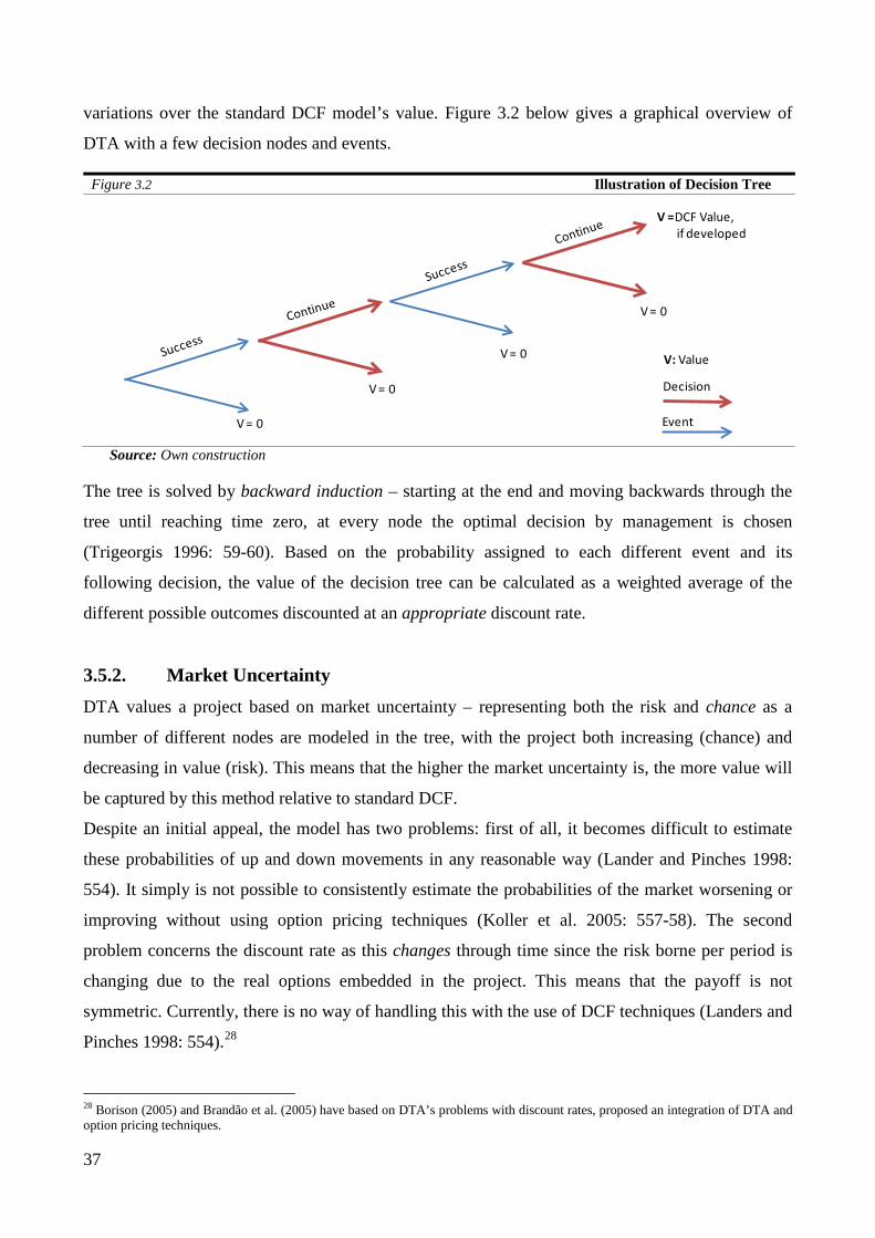
37

variations over the standard DCF model’s value. Figure 3.2 below gives a graphical overview of

DTA with a few decision nodes and events.

Figure 3.2 Illustration of Decision Tree


The tree is solved by backward induction – starting at the end and moving backwards through the

tree until reaching time zero, at every node the optimal decision by management is chosen

(Trigeorgis 1996: 59-60). Based on the probability assigned to each different event and its

following decision, the value of the decision tree can be calculated as a weighted average of the

different possible outcomes discounted at an appropriate discount rate.

3.5.2. Market Uncertainty DTA values a project based on market uncertainty – representing both the risk and chance as a

number of different nodes are modeled in the tree, with the project both increasing (chance) and

decreasing in value (risk). This means that the higher the market uncertainty is, the more value will

be captured by this method relative to standard DCF.

Despite an initial appeal, the model has two problems: first of all, it becomes difficult to estimate

these probabilities of up and down movements in any reasonable way (Lander and Pinches 1998:

554). It simply is not possible to consistently estimate the probabilities of the market worsening or

improving without using option pricing techniques (Koller et al. 2005: 557-58). The second

problem concerns the discount rate as this changes through time since the risk borne per period is

changing due to the real options embedded in the project. This means that the payoff is not

symmetric. Currently, there is no way of handling this with the use of DCF techniques (Landers and

Pinches 1998: 554).28

28 Borison (2005) and Brandão et al. (2005) have based on DTA’s problems with discount rates, proposed an integration of DTA and option pricing techniques.

Event

Decision

V = 0

V = 0

V = 0

V = 0

V =DCF Value,if developed

V: Value

38

3.5.3. Flexibility Where ENPV only modeled events based on development success or failure, DTA is also able to

handle the market uncertainty influencing project value. This difference makes it possible to model

decisions in the company based on new market information. The analysis thus helps to understand

the value which can be created by actively managing projects, instead of holding them passively.

When applying the method it is however important that the adjustments made to probabilities and

discount rates are clearly separated otherwise it can lead to uncertainties being mixed.

3.5.4. Usability While the calculations of DTA are relatively simple, the estimation of the inputs is difficult. It is

difficult to clearly separate market uncertainty and events in the modeling and currently not possible

to estimate the discount rate correctly, seriously limiting its use. Despite the limitations of the

decision tree, the model has its merits when it comes to information. If the need for a precise

estimate can be sacrificed, the strategic value of the process can be high, as the decision tree

demands identification of critical value drivers and decisions for the project.29 In this sense it can be

seen as bridging strategy and finance.

3.5.5. Decision Tree Overview

Table 3.4 Decision Tree Analysis Criteria



Project Scenarios and decisions Probability of event Yes



Risk and Chance Beta and discount rate adjustment due to option Not possible

If imprecision is accepted then it can be meaningful

for strategy


29 Lander and Pinches (1998: 554) make the argument that in many cases decision trees and real option valuation will lead to the same optimal strategy but with two different value estimates.

39

3.6 Real Options Valuation After our review of the DCF based valuation models, we now focus on real options valuation

(ROV). ROV takes its offset in the progression in the 1970s, where Black, Scholes and Merton

(1973) successfully developed models that could value financial options. This led Myers (1977) to

suggest that corporate assets could be perceived as “real options” to invest, grow or abandon.

Despite its promising features, ROV is still not a commonly used valuation technique. We will

therefore discuss its theoretical underpinnings as well as its practical value and lack of application.

3.6.1. Fundamentals Since Myers’ suggestion in 1977 a vast amount of both academic and practical literature has been

produced about ROV.30 The research about this valuation model has aimed at improving the

incorporation of the uncertainty of cash flows, and more importantly, to incorporate strategic

decision making in financial valuations. An extended list of the benefits of ROV is presented below.

- Getting management to ask the right questions.

- Assess the value of strategic choices.

- Expand the set of strategic alternatives that managers consider.

- Provide consistent comparison between financial market alternatives, internal investment opportunities and contracts.

- Acknowledge non-linear payoffs.

- Improved inclusion of uncertainty.

Source: Own construction, inspired by Amram and Kulatilaka 1999: 4-8

Before discussing ROV, it is necessary to gain a better understanding of what an option is. We do

this through a brief discussion of financial options.

3.6.1.1. Financial Options

A financial option is a derivate or a security, whose value is driven by the dynamics of an

underlying asset and time (Miller and Park 2002: 109). More specifically, an option is a contract,

which gives the buyer the right but not the obligation to buy (call) or sell (put) an underlying asset

(V), at a pre-specified exercise price (EX) on a fixed expiry date (European) or up until such date

(American). The payoff structure of an options thus depends on the value of the underlying asset, as

seen in Figure 3.3 below, where the one to the left is a call option and the one to the right a put

option and the blue line represents the profit from holding the option.

30 For two comprehensive literature reviews of main contributions to the real options field, see Lander and Pinches (1998) and Miller and Park (2002). For a compact review see Trigeorgis (1996: 2-3).

40

Figure 3.3 Option Payoff Diagram


The call option will be exercised in the case where the underlying asset exceeds the value of the

exercise price at the expiry date. In an opposite way, a put option will be exercised when the value

of the underlying asset is below the exercise price. This asymmetric payoff implies that the option

will capture any upside, but will never have a value below zero, as seen in the formulas below.

Formula 3.3 Intrinsic Option Value

Call: MAX [V-EX; 0] Put: MAX [EX-V; 0]

Source: Copeland and Antikarov 2003: 128

When purchasing an option the investor only pays the price of the option today, effectively buying

the underlying asset on credit. Option values therefore increase with the interest rate and the time to

maturity. Furthermore since the payoff is asymmetric, the value of the option will increase with the

underlying asset’s market uncertainty. It also means that the value of the option increases with time

due to the higher the probability of up (call) or down (put) movements in stock price. These features

of an option’s value drivers are summarized in Table 3.5.

Table 3.5 Option Value

Source: Brealey et al. 2006: 554-557

3.6.1.2. Real options

The logic of financial options can be “translated” to wind farms under development. By investing a

small amount today in the first development stage, a company effectively purchases an option to

31 The direct effects of an increase in interest rate and volatility on the option price is positive. There may however be indirect effects, such an increase in interest rates reducing the value of the underlying asset and thus the option value.

Share Price Share Price

Valu

e of

Cal

l (Lo

ng p

ositi

on)

Valu

e of

Put

(Lon

g po

sitio

n)

Exercise Price

Exercise Price

Call Option Put Option

Increase in: Change in Call Option Value Change in Put Option ValueValue of Underlying Asset (V) Positive NegativeExercise Price (EX) Negative Positive Interest Rate (r f ) Positive NegativeTime to Maturity (t) Positive PositiveVolatility of V (σ) Positive Positive

41

continue development, given this stage is successful. If conditions turn out to be worse than

anticipated, the company can choose to walk away, only losing the upfront investment of

development. A real option can thus be defined as: the right but not the obligation, to take action in

(e.g. continuing or expanding) a project at a predetermined price (EX), up to the date when the

investment opportunity will cease to exist (Trigeorgis 1996: 124).

Whereas the standard DCF model assumes that the entire investment decision is taken today, ROV

keeps the decision “open” until the exercise date. In many (but not all) cases this adds a significant

value, but one of the following characteristics needs to be present for a ROV to be recommendable.

Future investment decisions contingent on uncertainty are necessary.

Uncertainty is so large that it is sensible to wait for new information to avoid regret of irreversible investment.

Value of project is future growth options rather than current cash flows.

When there will be project updates and mid-course strategy corrections.

When project costs are high and a large proportion can be avoided if project is terminated prematurely.

Value of project is close to zero.

Source: Amram and Kulatilaka (1999:24) and Willigers and Hansen (2008: 531)

These characteristics show that ROV should not be applied to all projects. To apply ROV, a

strategic analysis of the project is often necessary to determine the possible options. This analysis

can provide many qualitative insights and can be referred to as the strategic value of ROV (Villiger

and Bogdan 2005a: 428). Despite these financial and strategic potentials of ROV, the question still

remains if (financial) option pricing techniques can be justifiably used on real assets due to the

differences seen in Table 3.6.

Table 3.6 Difference Between Real and Financial Options

Source: Own construction, inspired by Kodukula and Papudesu 2006: 2-3

Financial Options Real OptionsValue of Underlying Asset (V) Stock price Present value of operational projectOption Price (OV) Fixed on financial market Initial project investment Exercise Price (EX) Fixed value in option contract Cost of realizing option/projectTime to maturity (t) Fixed in contract Not always clearly knownVolatility(σ) Volatility of the stock price Volatility of the project

Increase in time to maturity Value increases Value should increase but this might be diminished by entry of competitors

Option holder’s control of value None Management can influence option value.

Increase in volatility Value increases Value increases

Resolution of uncertainty Clears continuously through time Can be necessary to invest for more information – can be cleared in lumps

Liquidity Complete market Very low/complex

Rationality behind exercise Rational Exercise can have political or personal implications.

42

These differences between real and financial options, are included both in our theoretical discussion

and in our implementation of ROV on a wind farm under development. We will start below with the

most controversial assumption of ROV: the market completeness assumption.

3.6.1.2.1. The Market Completeness Assumption and the Underlying Asset Value

For option pricing techniques to be correct, the assumption of no-arbitrage must hold. This means

that markets are assumed to be complete, so that every future market state can be replicated in a

portfolio using already existing assets (Smith and Nau 1995: 802). In the case of financial options

this portfolio can be constructed using the underlying traded stock. Whether a similar approach can

be applied to real options is a question of much debate, and where the real option analogy is most

often challenged (Shockley and Arnold 2003: 82).

The question is raised due to the fact that the investment projects, which make up the underlying

asset, are generally regarded as being untradeable or tradable only at substantial costs and on

incomplete markets (Trigeorgis 1996: 128). The question was already discussed by Mason and

Merton (1985: 38-39). They point to the fact that DCF models also rest on a complete market

assumption. In spite of this, DCF models are often used for non-traded projects, where the cost of

equity is estimated from a traded twin-security that has the same risk profile, the beta. The

assumption is therefore no stronger in ROV than in the DCF models (Trigeorgis 1996: 127).

A similar point is found in Shockley and Arnold (2003: 87-88): “corporate finance involves the

application of financial market pricing mechanisms to illiquid corporate investments”. Valuation

models will thus not provide entirely precise results in many cases. However, the models should be

evaluated according to their ability to give good predictions and assist decisions and here ROV is

superior to DCF in situations of high uncertainty. Based on these arguments, it is therefore

recommended to use the project itself as the underlying asset of the ROV.

To use the project itself as the underlying asset, it is necessary to find a value of this asset without

options (equal to it being a stock). Copeland and Antikarov (2003: 94) argue that the best way of

doing this is to calculate the NPV of the project with no flexibility using the standard DCF model as

this serves as the best unbiased estimate of the market value of the real asset, if it were traded. They

call this the Marketed Asset Disclaimer (MAD). Based on these arguments the value of real options

can be found using the models originally developed for financial options.

3.6.1.3. Option Pricing Models

A long range of different models exist for pricing options such as continuous-time models including

the Black-Scholes model, finite difference scheme models and lattice models (Lander and Pinches

43

1998: 543-47). In the practical real option literature the binomial model and the Black-Scholes

model have been given the majority of the attention.

3.6.1.3.1. The Black-Scholes Model32

The Black-Scholes model is built upon some very strong assumptions that make it difficult to apply

correctly in ROV. In some cases the formula can be modified to handle, for example, dividends,

stochastic volatility, or interest rates. However, for investment opportunities with non-standard

features, the Black-Scholes model will not work. These non-standard features include options with

multiple uncertainties, American options or options known as compound options (Lander and

Pinches 1998: 543-44). Since a wind farm under development is subject to these features, the model

is therefore not recommended. We thus focus on the binomial model, as it is the most applied model

for the challenges that we face.

3.6.1.3.2. The Binomial Model

As outlined in chapter 2, the development phase of a wind farm is divided into several stages. When

a stage is completed, the investor has the right, but not the obligation, to continue development. If

he chooses to continue, he will enter the next stage. Thus the development phase does not consist of

a single option, but several options. Such a multistage option is called a compound option. To value

a compound option, the practical real option literature generally suggests the binomial model.33

The binomial model is a discrete time simulation of the value of the underlying asset, which models

the different possible values that the underlying asset can take over the life of the option in a

binomial tree (Hull 2008: 237). It assumes that the value of the underlying asset (V0) follows the

binomial distribution and, for every time step (∆t), it can take one of two values, either increasing

(u) or decreasing (d). As time steps become smaller in this model, the movements of the underlying

asset will approach the normal distribution and the binomial model actually has the Black-Scholes

model as a special limiting case. A two-step example of a binomial tree is illustrated below:

32 For more details on the Black-Scholes model we refer to Appendix 8. 33 Other methods exist for valuing compound options including Geske’s model (1979) and Schwartz’ least-squares Monte Carlo model (2004). These models do however lack the intuitive appeal of the binomial model and are rarely seen in the practical literature. They will therefore be disregarded in line with this thesis’ limitations.

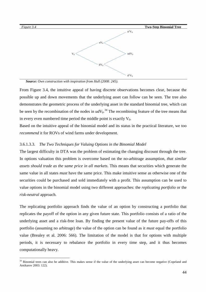
44

Figure 3.4 Two-Step Binomial Tree

Source: Own construction with inspiration from Hull (2008: 245).

From Figure 3.4, the intuitive appeal of having discrete observations becomes clear, because the

possible up and down movements that the underlying asset can follow can be seen. The tree also

demonstrates the geometric process of the underlying asset in the standard binomial tree, which can

be seen by the recombination of the nodes in udV0.34 The recombining feature of the tree means that

in every even numbered time period the middle point is exactly V0.

Based on the intuitive appeal of the binomial model and its status in the practical literature, we too

recommend it for ROVs of wind farms under development.

3.6.1.3.3. The Two Techniques for Valuing Options in the Binomial Model

The largest difficulty in DTA was the problem of estimating the changing discount through the tree.

In options valuation this problem is overcome based on the no-arbitrage assumption, that similar

assets should trade as the same price in all markets. This means that securities which generate the

same value in all states must have the same price. This make intuitive sense as otherwise one of the

securities could be purchased and sold immediately with a profit. This assumption can be used to

value options in the binomial model using two different approaches: the replicating portfolio or the

risk-neutral approach.

The replicating portfolio approach finds the value of an option by constructing a portfolio that

replicates the payoff of the option in any given future state. This portfolio consists of a ratio of the

underlying asset and a risk-free loan. By finding the present value of the future pay-offs of this

portfolio (assuming no arbitrage) the value of the option can be found as it must equal the portfolio

value (Brealey et al. 2006: 566). The limitation of the model is that for options with multiple

periods, it is necessary to rebalance the portfolio in every time step, and it thus becomes

computationally heavy.

34 Binomial trees can also be additive. This makes sense if the value of the underlying asset can become negative (Copeland and Antikarov 2003: 122).

V0

uV0

dV0

u2V0

udV0

d2V0

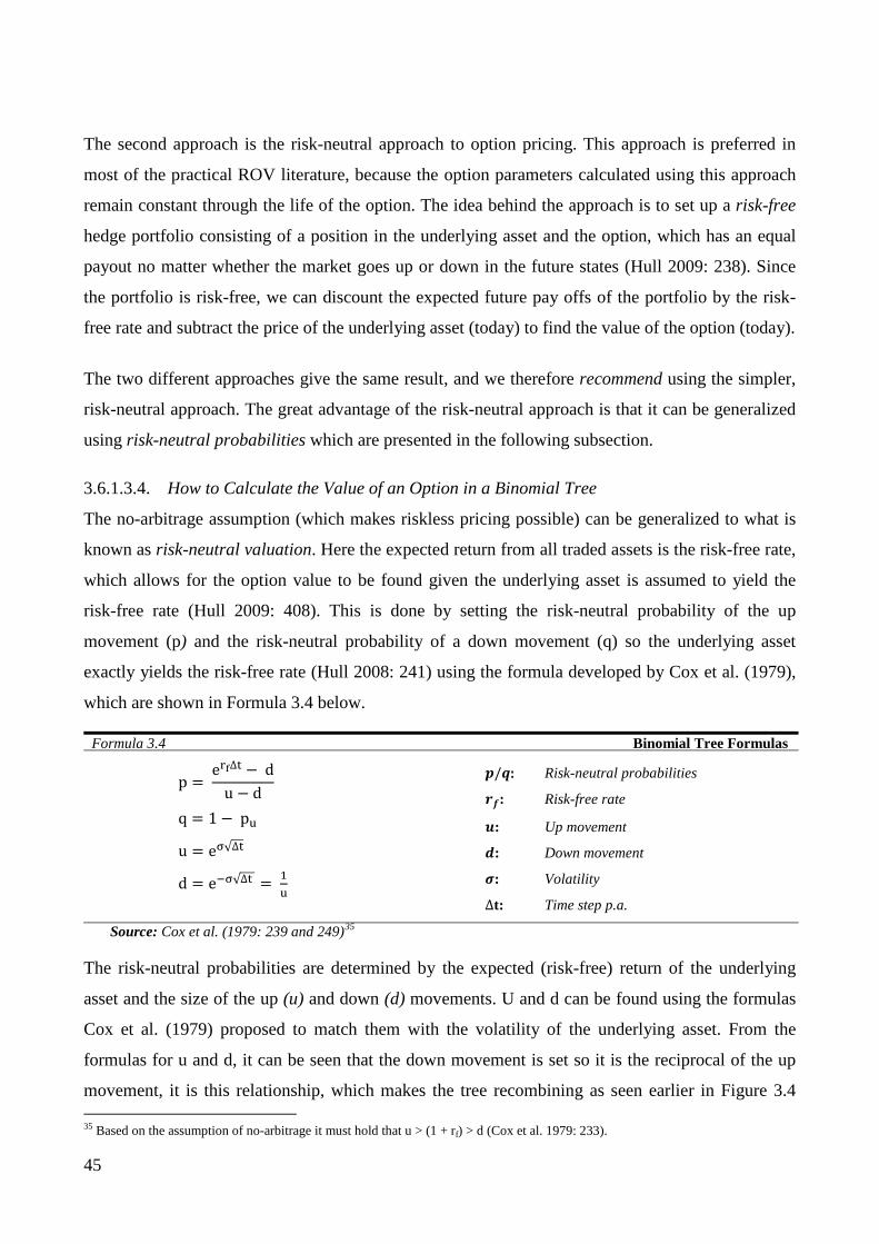
45

The second approach is the risk-neutral approach to option pricing. This approach is preferred in

most of the practical ROV literature, because the option parameters calculated using this approach

remain constant through the life of the option. The idea behind the approach is to set up a risk-free

hedge portfolio consisting of a position in the underlying asset and the option, which has an equal

payout no matter whether the market goes up or down in the future states (Hull 2009: 238). Since

the portfolio is risk-free, we can discount the expected future pay offs of the portfolio by the risk-

free rate and subtract the price of the underlying asset (today) to find the value of the option (today).

The two different approaches give the same result, and we therefore recommend using the simpler,

risk-neutral approach. The great advantage of the risk-neutral approach is that it can be generalized

using risk-neutral probabilities which are presented in the following subsection.

3.6.1.3.4. How to Calculate the Value of an Option in a Binomial Tree

The no-arbitrage assumption (which makes riskless pricing possible) can be generalized to what is

known as risk-neutral valuation. Here the expected return from all traded assets is the risk-free rate,

which allows for the option value to be found given the underlying asset is assumed to yield the

risk-free rate (Hull 2009: 408). This is done by setting the risk-neutral probability of the up

movement (p) and the risk-neutral probability of a down movement (q) so the underlying asset

exactly yields the risk-free rate (Hull 2008: 241) using the formula developed by Cox et al. (1979),

which are shown in Formula 3.4 below.

Formula 3.4 Binomial Tree Formulas

p = erf∆t − d

u − d

q = 1 − pu

u = eσ√∆t

d = e−σ√∆t = 1u

𝒑/𝒒: Risk-neutral probabilities


𝒖: Up movement

𝒅: Down movement

𝝈: Volatility

∆t: Time step p.a.

Source: Cox et al. (1979: 239 and 249)35

The risk-neutral probabilities are determined by the expected (risk-free) return of the underlying

asset and the size of the up (u) and down (d) movements. U and d can be found using the formulas

Cox et al. (1979) proposed to match them with the volatility of the underlying asset. From the

formulas for u and d, it can be seen that the down movement is set so it is the reciprocal of the up

movement, it is this relationship, which makes the tree recombining as seen earlier in Figure 3.4 35 Based on the assumption of no-arbitrage it must hold that u > (1 + rf) > d (Cox et al. 1979: 233).

46

(Copeland and Antikarov 2003: 121-122). In the formula σ is the annual volatility of the return,

which is adjusted for the amount of time steps per year. Having found the risk-neutral probabilities

and up and down movements, we can then in the risk-neutral world find the present value of our

option in each binomial node by using the below formula.

Formula 3.5 Option Value in Binomial Tree

OV0 = [pOVu+(1−p)OVd]erf∆t

𝑶𝑽𝟎: Present value of option

𝑶𝑽𝒖/𝒅: Value of option in future up/down state

𝒑: Risk-neutral probability


∆𝒕: Length of time steps given in years

Source: Cox et al. (1979: 237)

The formula states that the value of the option today (OV0) is its expected pay-off (OVu or OVd) in

a risk-neutral world, discounted at the continuously compounded risk-free rate (Hull 200: 241). To

find the value of the option in the binomial tree, we therefore start by building the asset value tree

(previously demonstrated in Figure 3.4), with the value of the underlying asset moving up and

down. Based on this asset value tree, we use Formula 3.5 to find the present value of the option by

solving it recursively. This has been done in Figure 3.5 below for a European call option, where the

exercise price (EX) has been subtracted to find the expected pay-off in the final nodes, which is

then discounted to find the present value.

Figure 3.5 Option Value Tree for a Two Period European Call

s


The main advantage of calculating the value of the underlying asset and options this way is that the

option parameters remain constant, and that the development in price of the option, as well as the

underlying asset, is observable, which gives an intuitive appeal.

Solved Recursively

OV3 = Max [u2V0-EX;0]

OV4 = Max [udV0-EX;0]

OV5 = Max [d2V0-EX;0]

[pOV1+qOV2]erf∆tOV0 =



47

However, a formula for valuing options based on investors being risk-neutral can be contra-intuitive

for many managers, and might pose a problem for the acceptance of the model (Lander and Pinches

1998: 546). To understand this better, it is important to emphasize that we are not valuing the option

in absolute but in relative terms. The price of the option is valued relative to the value of the

underlying asset (V0), its movements (u and d) and rf – variables, which can be affected by the risk

attitudes of investors (Cox et al. 1979: 235). To further expand the intuition behind the model we

discuss its underlying assumptions in more details below.

3.6.1.3.5. The Underlying Assumptions of the Binomial Model

A vast amount of extensions to the above presented binomial model exist in the options literature,

but the formulas above are the most common when applying the binomial model to ROV. They are

based on a range of assumptions such as σ and the rf being known and constant throughout the life

of the option. Other important assumptions of the model include: no transaction costs, unlimited

riskless lending and borrowing, no taxes and no margin requirements (Cox et. al. 1979: 233).

Finally, it is assumed that the value of the underlying asset follows a stochastic process known as a

geometric Brownian motion, i.e. that the underlying asset has random normally distributed

returns.36 This assumption (together with the assumption of a constant σ) is necessary for the

probability of up and down movements to remain constant throughout the model (Brandão et. al.

2005: 74). These assumptions mean that information is perceived as arriving continuously in a

smooth and consistent way, so the value of the underlying asset does not make any large jumps. But

in the case of wind farms under development, the information about events does not arrive in such a

way. The binomial model can handle such situations using what Copeland and Antikarov (2003:

281) call the quadranomial approach or two-variable binomial tree. In such situations it becomes

clear, that the underlying assumptions of the binomial model are violated and the results of the

model become less precise (Shockley 2007: 237). But (as discussed) earlier it goes for the valuation

models that all the assumptions of the models will never be fulfilled, when dealing with real assets

and the values obtained are indicative and not exact. Based on this thorough introduction of the

fundamental theory underlining ROV, we will now discuss it in relation to the three other criteria

we have defined.

36 Other processes can also be handled in the binomial model such as the arithmetic Brownian motion and mean-reverting Ohrnstein-Uhlenbeck processes (Brandão et al. 2005: 84-85).

48

3.6.2. Market Uncertainty In ROV market uncertainty is seen as the possibility that the value of the underlying asset moves

either up (chance) or down (risk) from the initial value. Graphically the real option way of thinking

market uncertainty is illustrated in Figure 3.6.

Figure 3.6 The Cone of Uncertainty and Two Random Price Paths

Source: Amram and Kulatilaka 1999: 15-16

The underlying asset has a value at time 0 (V0). This value is uncertain over time, and has a chance

of moving up and a risk of moving down and as such it can develop within the “Cone of

Uncertainty”, which shows that the uncertainty increases with time. But if we purchase a call

option today (OV0), the maximum possible loss we can experience is the price of the option today.

While we have a limited downside we are able to take advantage of any potential upside pay-off.

The asymmetric pay-off leads to a fact that might seem contra-intuitive, that more market

uncertainty increases the value of a project. This means that in a situation where a manager has to

chose between two projects with equal expected returns, the one with the highest volatility should

be chosen (Miller and Park 2002: 128). It is however important to emphasize that for uncertainty to

have the above features, it needs to be resolved on a continuous basis so that management can react

to the outcome.

The market uncertainty estimate in ROV is the volatility σ expressing the uncertainty an asset is

exposed to from being on the market (Copeland 2003: 245). Market uncertainty should not be

confused with the concept of market risk as defined previously in the DCF models, as it differs in

two ways. First, market uncertainty includes both risk and chance. Second, market uncertainty is the

total uncertainty from being on the market, i.e. described in DCF terminology; it includes both

diversifiable and non-diversifiable risk.

OV0

V0

OVu = Max(VU-EX;0)

Value

Time

OVd = Max(VD-EX;0)

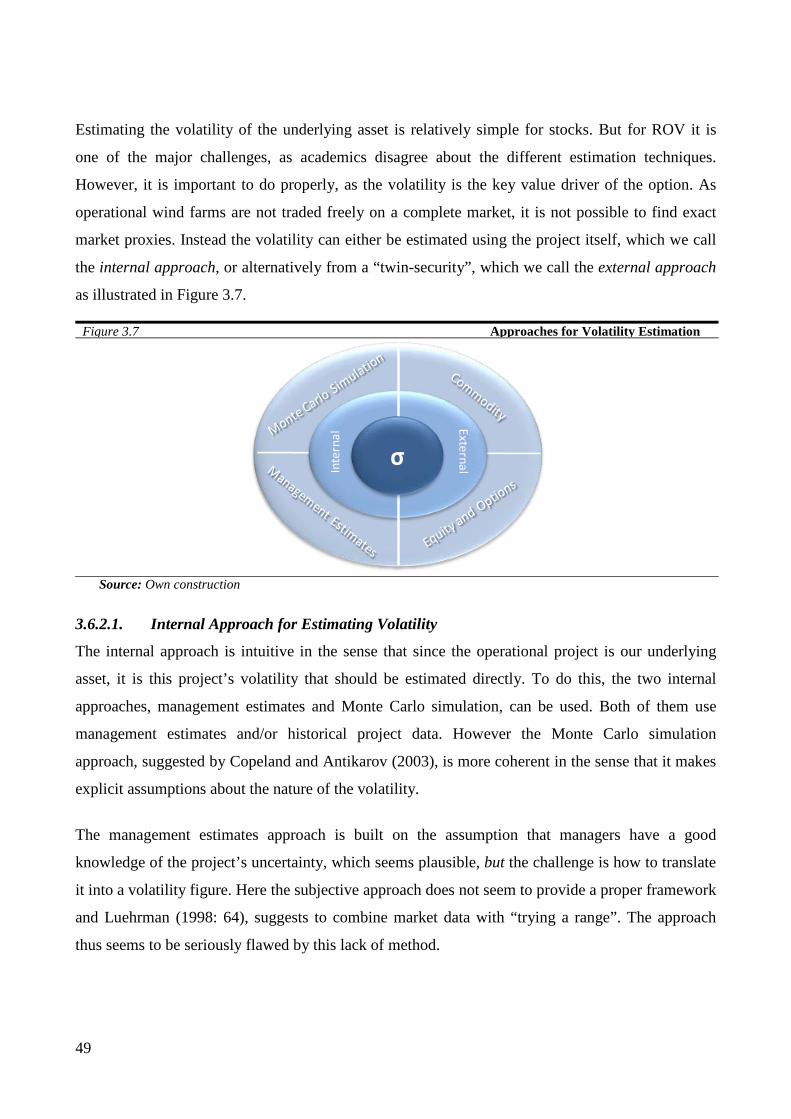
49

Estimating the volatility of the underlying asset is relatively simple for stocks. But for ROV it is

one of the major challenges, as academics disagree about the different estimation techniques.

However, it is important to do properly, as the volatility is the key value driver of the option. As

operational wind farms are not traded freely on a complete market, it is not possible to find exact

market proxies. Instead the volatility can either be estimated using the project itself, which we call

the internal approach, or alternatively from a “twin-security”, which we call the external approach

as illustrated in Figure 3.7.

Figure 3.7 Approaches for Volatility Estimation


3.6.2.1. Internal Approach for Estimating Volatility

The internal approach is intuitive in the sense that since the operational project is our underlying

asset, it is this project’s volatility that should be estimated directly. To do this, the two internal

approaches, management estimates and Monte Carlo simulation, can be used. Both of them use

management estimates and/or historical project data. However the Monte Carlo simulation

approach, suggested by Copeland and Antikarov (2003), is more coherent in the sense that it makes

explicit assumptions about the nature of the volatility.

The management estimates approach is built on the assumption that managers have a good

knowledge of the project’s uncertainty, which seems plausible, but the challenge is how to translate

it into a volatility figure. Here the subjective approach does not seem to provide a proper framework

and Luehrman (1998: 64), suggests to combine market data with “trying a range”. The approach

thus seems to be seriously flawed by this lack of method.

Inte

rnal

Externalσ

50

It is exactly this problem of quantifying management knowledge into market uncertainty, which

Copeland and Antikarov (2003: 260) propose a framework for. This is done by quantifying the

uncertainty of all (market) variables that influence the volatility of the project’s cash flow and

consolidating them into a single figure (σ) using a Monte Carlo simulation.37 The approach is built

on two explicit assumptions. The first is the MAD assumption presented previously, which makes it

reasonable to focus on the project’s volatility, as the project is the underlying asset. The second

assumption is that based on Samuelson’s proof (1965) that properly anticipated prices fluctuate

randomly, it is possible to combine any number of uncertainties in a Monte Carlo simulation and

assume that they follow a random walk when combined (Copeland and Antikarov 2003: 219).

While the assumptions might be strong, the actual implementation of the Monte Carlo simulation is

even more problematic with regard to the estimation of the individual uncertainties and their

autocorrelations and intercorrelations in time. Copeland and Antikarov discuss these issues, but are

not very explicit in their practical examples on how these can be estimated, nor do they properly

explain how the probability distributions of the different variables should be chosen. This is

problematic because defining probability distributions, autocorrelations, and intercorrelations, of

variables is a difficult task and as such the simulation easily becomes a black box.38 This has two

problematic implications. First, as it is unlikely that the inputs will be precise, then the method

could lead to large mistakes in estimation of volatility, secondly since capital budgeting is not

always impartial, the opaque estimation technique could disguise biased estimates. Combined these

arguments make the method unattractive for estimation of the market uncertainty of wind farms and

it is therefore not recommended.

3.6.2.2. External Approach for Estimating Volatility

Having discarded the internal approaches, we turn to the external ones to see if these can provide a

reasonable estimate for the volatility of our underlying asset. The idea to use a market proxy to

estimate the volatility of the project can be seen as the “classic” way of estimating the volatility of

the project (Borison 2005: 18). Miller and Park (2002: 124) argue that for commodity based

projects it is possible to use the commodity price to find a reasonable proxy for the volatility.39 The

argument by Miller and Park of finding the commodity price volatility is supported by the fact that

several classic commodity ROV texts such Brenan and Schwartz (1985: 154) and Dixit and Pindyck

37 Copeland and Antikarov (2003: 270) are unclear on what to include in the estimation of market uncertainty, only stating that individual uncertainties resolved in a non-continuous way should not be included as input in the Monte Carlo simulation. 38 These problems are also clear from Brandão et al. (2005: 80) and Méndez et al. (2009: 7-8) who use the method, but only briefly discuss distributions without mentioning possible autocorrelations or interrelations. 39 This approach has also been suggested by Copeland et al. (1994: 543). Copeland’s change of position thereby clearly demonstrates the work-in-progress of volatility estimation within ROV.

51

(1994: 179) use commodity price volatility as an expression of the market uncertainty of the project.

This is also the case for several of the articles we have found, which apply ROV to the valuation of

renewable energy projects, such as Bøckman et al. (2007: 257), Fleten et al., (2007: 2) and

Venetsanosa et al. (2002: 10). The alternative external approach would be to use either historical or

implied stock volatilities, as seen in Willigers and Hansen (2008: 532). They are, however,

performing the calculations for pharmaceutical projects and therefore do not have the commodity

option. This furthermore requires that the publicly traded company has the same risk profile as the

project considered, thereby posing a serious limitation to this estimation technique.

Despite a commodity is unlikely to give an entirely precise estimate of project volatility, it is

recommended for wind farms under development. This is based on its advantage of using

observable market data, its intuitive appeal and it being used by others academics in ROVs of

commodity based projects.

3.6.2.3. The Stochastic Process of the Market Uncertainty

To describe the evolution in value over time of the underlying asset, different option pricing models

apply different stochastic processes. In the ROV literature, the stochastic process has been treated

by Smith and McCardle (1997: 6) and Laughton and Jacoby (1995: 199), with the conclusions that

the assumption of the underlying stochastic process has a major impact on the value and decisions

undertaken.

A stochastic process is defined as a variable that evolves over time in a way that is at least partly

random. One of the simplest examples of such a stochastic process is the random walk, which

formalizes the idea of independent successive steps in random directions (Dixit and Pindyck 1994:

60-61). Such a random walk is a Markov process (i.e. it satisfies the Markov property). This has a

great advantage, as it implies that only current information is useful for forecasting the future path

of the process, thereby simplifying the analysis (Dixit and Pindyck 1994: 63).

The geometric Brownian motion is the most applied and well known of the stochastic processes and

serves as the basis for the Black-Scholes model and is the process which the binomial model

approximates as the amount discrete time steps increase. One of the reasons for its popularity is its

relatively simplicity and also that it does not allow the price of a given asset to fall below the value

of zero. Formally the geometric Brownian motion is a continuous-time stochastic process, with a

non-random (i.e. deterministic) drift and a constant volatility which varies with the stochastic

Brownian motion (Blanco et al. 2001: 76). However when modeling commodity prices it has been

52

suggested that the geometric Brownian motion is not appropriate (Blanco et al. 2001: 80). This

critique will be discussed in further detail in chapter 4.

3.6.3. Flexibility As we have seen, the standard DCF model and ENPV are unable to value decisions. The real

options model in many ways offers a solution to these issues, as it can model the active decisions of

the management based on both the market uncertainty described above and the events during the

development phase.

While the market uncertainty is included through the volatility, the events cannot be handled in a

standard binomial model. Some authors, such as Myers and Majd (1990), have combined the two

into a single figure depicted by volatility. To adopt such an approach, the events and the market

uncertainty need to follow the same stochastic process, which is clearly wrong for wind farms under

development. Instead it has been suggested that the events are modeled similar to the ENPV

approach as event probabilities. To do this, it is necessary to expand the binomial model using what

is known as the quadranomial approach (Copeland and Antikarov 2003: 279). This approach will

be demonstrated in chapter 4. The decisions are included in the valuation of a project as the

different types of real options in a project, discussed below.

3.6.3.1. Types of Real Options

Many different types of options can be present when using ROV, so it is necessary to know and

understand the different option types. In Table 3.7 we describe the most common real options.

Table 3.7 Common Real Options

Type Description Simple Options Option to defer Option to wait with execution of investment decision. Option to continue Option to continue development Option to alter scale Option expand, contract, shut down and restart production. Option to abandon Option to abandon current operations permanently for salvage value. Option to switch Option change output or input mix of a production. Growth option Platform investment which makes it possible to grow given new innovations. Compound Options Parallel compound option Various options alive at the same time Staged compound option Option whose value is dependent on a previous option being exercised Concurrent compound option Options whose value is dependent on a parallel option not being exercised Advanced Options Rainbow option Option with more than one source of uncertainty

Learning option (Rainbow) option where market uncertainty is increasing through time and technological uncertainty (events) is resolved through time.

Source: Trigeorgis 1996: 2-3 and Copeland and Antikarov 2003: 12 and 221.

53

As we have stated earlier, a wind farm under development should be perceived as a staged

compound option, as each future stage depends on the previous option being exercised. The staged

compound option is distinct compared to the other compound options because only one option is

alive at a time. This means that the value can be calculated as the sum of the different options

through time (Shockley 2007: 350). In the case of either multiple interacting or concurrent options,

the calculation becomes more complicated, since the value of these cannot be found simply as the

addition of all the different option values. This means that the incremental value of adding an extra

option is decreasing, also known as the diminishing option value effect (Trigeorgis 1996: 227). The

most important action is therefore to identify and value the most crucial option(s) instead of

including every possible option, as this easily induces more complexity and model problems than is

added in precision and explanatory power (Skjødt 2001: 44). It is important to recognize that a

ROV is only a valuation at a given point in time, which can help the explicitation of different

scenarios and decisions, but it can never cover all future contingencies.

3.6.4. Usability Even though ROV in many ways presents an intuitive perspective on investment decision valuation,

it is still not a widely accepted framework in practical business life (Copeland and Antikarov 2003:

VIII). The reason for this seems to be a combination of doubts about the underlying assumptions

(Shockley and Arnold 2003: 87) and the increased complexity of the estimation and calculation,

which leads to lack of trust among managers (Hartmann and Hassan 2006: 353).

The critique of ROV’s unrealistic assumptions is flawed in the sense that the assumptions are no

stronger than those used in many DCF valuations. Instead we believe that the critique of the

assumptions is based partly on its relative youth and because its assumptions are more explicit than

in the standard DCF model. The relative youth of the method also applies to the point emphasizing

ROV’s difficulty of use, as it means that corporations have little experience with the method,

leading to uncertainty about estimation and calculation methods. This is reflected by many

practitioners finding that the current tools are too complex in use, and that the real option literature

should focus more on developing viable and practical solutions instead of model fine tuning (Miller

and Park 2002: 129). A problem exacerbated by the fact that there still is no standard ROV model,

and with the different models criticizing each other, the reluctance of practitioners is

understandable.

It is clear that as long as the calculations are deemed to be either too difficult and/or non-

transparent, then a meaningful interpretation of the results is not possible. However, a big advantage

with regard to interpretation of results is the thought process behind sketching out the options and

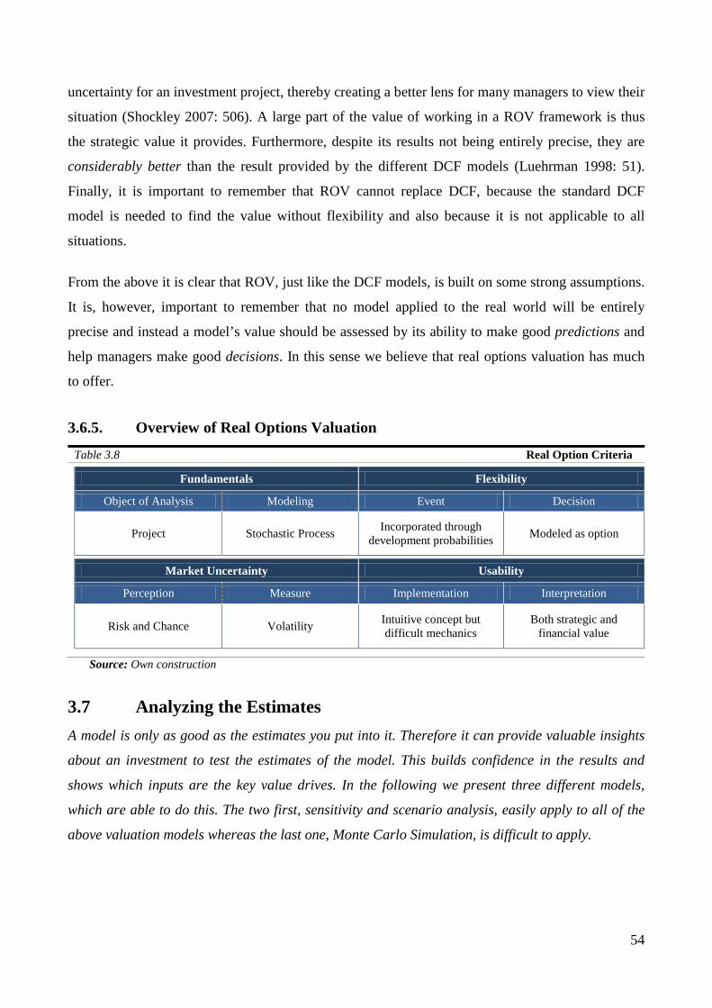
54

uncertainty for an investment project, thereby creating a better lens for many managers to view their

situation (Shockley 2007: 506). A large part of the value of working in a ROV framework is thus

the strategic value it provides. Furthermore, despite its results not being entirely precise, they are

considerably better than the result provided by the different DCF models (Luehrman 1998: 51).

Finally, it is important to remember that ROV cannot replace DCF, because the standard DCF

model is needed to find the value without flexibility and also because it is not applicable to all

situations.

From the above it is clear that ROV, just like the DCF models, is built on some strong assumptions.

It is, however, important to remember that no model applied to the real world will be entirely

precise and instead a model’s value should be assessed by its ability to make good predictions and

help managers make good decisions. In this sense we believe that real options valuation has much

to offer.

3.6.5. Overview of Real Options Valuation

Table 3.8 Real Option Criteria



Project Stochastic Process Incorporated through development probabilities Modeled as option



Risk and Chance Volatility Intuitive concept but difficult mechanics

Both strategic and financial value


3.7 Analyzing the Estimates A model is only as good as the estimates you put into it. Therefore it can provide valuable insights

about an investment to test the estimates of the model. This builds confidence in the results and

shows which inputs are the key value drives. In the following we present three different models,

which are able to do this. The two first, sensitivity and scenario analysis, easily apply to all of the

above valuation models whereas the last one, Monte Carlo Simulation, is difficult to apply.

55

3.7.1. Sensitivity Analysis and Scenario Analysis Sensitivity analysis uses the estimates and the value found with the previous presented models, and

then simply tests the impact of changing one variable, while assuming all other variables are

constant (Bessis 2002: 79). The analysis thus tells us what the consequence on the value of the

project is, if there is a variation or misestimation in a variable (Trigeorgis 1996: 53). It thereby

supports management in determining the most crucial variables for the value of a project.40 The

simplicity of the sensitivity analysis is its strength as well as its weakness. The problem is that in

most cases if one variable changes, the others are likely to do so as well, but such interrelations of

errors or variances is not considered in the analysis. This can be considered through scenario

analysis, which creates a number of alternative scenarios with different (but consistent) sets of

variables. The scenario analysis can in this sense give management of good view of the situations,

thereby providing valuable information.41

However, neither analysis accounts for the serial dependency of estimates, which could lead to

errors growing through time (Trigeorgis 1996: 54). Furthermore “pessimistic” or “optimistic”

variations are often based on some sort of subjective assessment and it can be hard to interpret their

meaning. Finally, they both lack a clear decision rule and there is no way to reconcile, aggregate or

choose between different scenarios (Amram and Kulatilaka 1999: 39).

3.7.2. Monte Carlo Simulation Monte Carlo simulation tries to address both the interdependency of the different variables, the

serial dependency and potentially also the subjectivity of the estimates. A Monte Carlo simulation is

able to inspect the entire distribution of outcomes considering all possible combinations of the

variables. This is based on repeated random sampling from the probability distributions for each of

the crucial variables underlying the cash flows of a project. From this, a probability distribution of

the cash flows or the NPV of the project can be created (Trigeorgis 1996: 54).

A Monte Carlo simulation is a powerful tool for management, as it addresses several of the

problems of scenario and sensitivity analysis. Furthermore, it shows management an entire range of

values instead of giving them just a few pessimistic or optimistic estimates. Despite the promising

features of a Monte Carlo simulation, it is prone to a number of problems. Many of these concern

the technical issues of the simulation as discussed earlier. Trigeorgis (1996: 56) criticizes the

40 Often sensitivity analysis is used as break-even analysis, studying how low a given variable can become before project NPV is 0 (Brealey et al. 2006: 249). 41 Scenario analysis can also be used to stress test a given project or company, where all relevant variables take “worst-case” values (Bessis 2002: 78).

56

creation of many different present values for the project, as price then can no longer be interpreted

as the value of the project given competitive capital markets, thus making it unclear what the value

represents. In general, the results of a simulation, although providing a good overview of

uncertainty, are not intuitively interpreted. Finally, the largest difficulty of the model is that the

simulation is based on a forward looking predetermined strategy. It is thus unable to handle

decisions and provides no clear investment decision rule.

While it is clear that these analyses can test the estimates of the different valuation models, they too

are subject to the notion that models are never be better than what you put into them. This is

especially true for the Monte Carlo simulation, which despite its promising features is threatened by

bad estimations. The sensitivity analysis, on the other hand, might be simple, but so is its message

and it clearly shows management, where to focus the estimation effort, and thus helps to build

confidence in the results. We therefore recommend and use sensitivity analysis to analyze our

results in the following chapter.

3.8 Recapitulation In the beginning of this chapter we quoted Myers (1984a) for pointing toward the need for bridging

the gap between strategic decision making and finance. It was also argued that, since decisions can

actually be undertaken during the development phase of a wind farm, a valuation models that

includes strategic decision making is particularly relevant for this type of investments. Based on

these ideas we have thoroughly reviewed both the standard DCF model, ENPV model, DTA and

ROV. One of the key insights from this analysis was that despite ROV often being called

unrealistic, due to its market completeness assumption for illiquid assets, the standard DCF model

often makes the same assumption.

To be able to systematically examine all the models we built a framework of four criteria, which we

found particularly relevant for valuation models for wind farms under development. Each of our

four models was thereafter discussed according to this framework. We did however use the majority

of the effort on ROV based on the fact that this is the most complex model and is a newcomer

among valuation models, and therefore needs special attention. In the figure below, the different

models have been ranked according to their incorporation of flexibility and market uncertainty, as

well as their ease of use. The fundamental criterion has not been included, as it due to its complex

nature cannot meaningfully be quantified.

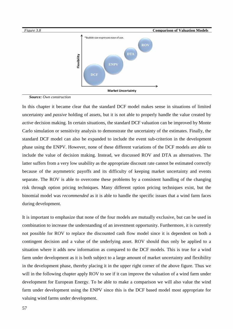
57

Figure 3.8 Comparison of Valuation Models


In this chapter it became clear that the standard DCF model makes sense in situations of limited

uncertainty and passive holding of assets, but it is not able to properly handle the value created by

active decision making. In certain situations, the standard DCF valuation can be improved by Monte

Carlo simulation or sensitivity analysis to demonstrate the uncertainty of the estimates. Finally, the

standard DCF model can also be expanded to include the event sub-criterion in the development

phase using the ENPV. However, none of these different variations of the DCF models are able to

include the value of decision making. Instead, we discussed ROV and DTA as alternatives. The

latter suffers from a very low usability as the appropriate discount rate cannot be estimated correctly

because of the asymmetric payoffs and its difficulty of keeping market uncertainty and events

separate. The ROV is able to overcome these problems by a consistent handling of the changing

risk through option pricing techniques. Many different option pricing techniques exist, but the

binomial model was recommended as it is able to handle the specific issues that a wind farm faces

during development.

It is important to emphasize that none of the four models are mutually exclusive, but can be used in

combination to increase the understanding of an investment opportunity. Furthermore, it is currently

not possible for ROV to replace the discounted cash flow model since it is dependent on both a

contingent decision and a value of the underlying asset. ROV should thus only be applied to a

situation where it adds new information as compared to the DCF models. This is true for a wind

farm under development as it is both subject to a large amount of market uncertainty and flexibility

in the development phase, thereby placing it in the upper right corner of the above figure. Thus we

will in the following chapter apply ROV to see if it can improve the valuation of a wind farm under

development for European Energy. To be able to make a comparison we will also value the wind

farm under development using the ENPV since this is the DCF based model most appropriate for

valuing wind farms under development.

DCF

ENPV

*Bubble size expresses ease of use.

Flex

ibili

ty

Market Uncertainty

DTA

ROV

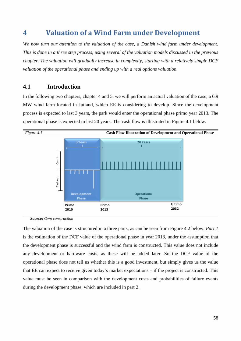
58

4 Valuation of a Wind Farm under Development We now turn our attention to the valuation of the case, a Danish wind farm under development.

This is done in a three step process, using several of the valuation models discussed in the previous

chapter. The valuation will gradually increase in complexity, starting with a relatively simple DCF

valuation of the operational phase and ending up with a real options valuation.

4.1 Introduction In the following two chapters, chapter 4 and 5, we will perform an actual valuation of the case, a 6.9

MW wind farm located in Jutland, which EE is considering to develop. Since the development

process is expected to last 3 years, the park would enter the operational phase primo year 2013. The

operational phase is expected to last 20 years. The cash flow is illustrated in Figure 4.1 below.

Figure 4.1 Cash Flow Illustration of Development and Operational Phase


The valuation of the case is structured in a three parts, as can be seen from Figure 4.2 below. Part 1

is the estimation of the DCF value of the operational phase in year 2013, under the assumption that

the development phase is successful and the wind farm is constructed. This value does not include

any development or hardware costs, as these will be added later. So the DCF value of the

operational phase does not tell us whether this is a good investment, but simply gives us the value

that EE can expect to receive given today’s market expectations – if the project is constructed. This

value must be seen in comparison with the development costs and probabilities of failure events

during the development phase, which are included in part 2.

Primo 2013

Development Phase

Operational Phase

Cash

out

Cash

in

3 Years 20 Years

Primo 2010

Ultimo 2032

59

Figure 4.2 Three Part Structure of Valuation in Chapters 4 and 5


The second part consists of three sections. First, the value of the development phase is estimated

including the events, using the ENPV model in section 4.3. Then, the market uncertainty is

introduced in section 4.4 using a binomial real options valuation, before these are combined in

section 4.5 using the quadranomial real options approach, giving us the value of the case, if all

equity financed.

The third part of the practical valuation concerns debt, and is performed separately in chapter 5 due

to the amount of new information that needs to be introduced. In chapter 4, only the value of the

investment decision is analyzed. As EE’s investment strategy is based on project finance a

significant amount of value is generated from the financing decision as well. Thus we value this

financing decision and finally determine the value of a wind farm under development.

Having outlined the progress in the chapter, we now start by valuing the operational wind farm.

4.2 DCF Value of Operational Phase To find the value of the operational phase, we apply the standard DCF model. This is the most

widely used model for valuing assets-in-place due to its simplicity and versatility. The valuation will

include an estimation and discussion of inputs such as costs, revenue, risk-free rate and cost of

equity. The result does not actually express the value of a wind farm under development but serves

as an input for the ENPV and ROV models.

Chapter Model Valuation of Include Debt Included?

Part 35 APV +

ROV Quadranomial

Development Phase +

Operational Phase

Events +Market Uncertainty Yes

Part 2

4.3

4.4

4.5

ENPV

ROV Binomial

ROV Quadranomial

Development Phase+

Operational Phase

Events

Market Uncertainty

Events +Market Uncertainty

No

No

No

Part 14.2 DCF Operational Phase N/A No

60

4.2.1. Four Step DCF Model The value of the wind farm’s operational phase using the DCF model is equal to the value of the

free cash flows (FCF) that the project generates. The model is easy applicable and the value will be

found in four steps, as presented in Figure 4.3 below.

Figure 4.3 The Four Step DCF Model


Step 1 is the estimation of the wind farm’s FCF. The step includes the estimation of expected

revenues and costs. Step 2 is an estimation of the appropriate cost of equity for the DCF model. In

Step 3 the DCF value of the wind farm is calculated. Step 4 is the interpretation of the results, which

in our case is strengthened by performing a sensitivity analysis.

4.2.2. Step 1: Estimating Free Cash Flows The FCF represents the cash flow generated by operations less any reinvestments back into the

business, and as such it represents the cash flows available to all investors and is independent of

leverage. The FCF thus represents the cash at disposal in a given period and is unlike net income

free of accounting measures. To find the FCF we need to set up a budget with each budget posts

containing a number of variables that need to be estimated, as seen in Table 4.1 below.

Step 1 Estimate Free

Cash Flows

Step 2 Estimate Cost of

Equity

Step 3 Estimate DCF

Value

Step 4 Sensitivity Analysis

61

Table 4.1 Estimating Free Cash Flow for Wind Farm

Budget Post Variables

1. Revenue

Tariff . Production =

a . (1-b) . c . d . e

Production:

a. Expected gross production

b. Grid loss

c. Park availability

Tariff:

d. Market price

e. Subsidy premium

2. Costs

Land lease

Insurance

Maintenance

Decommissioning costs

Own power consumption

3. EBITDA 1 – 2

4. Depreciation Accelerated depreciation at 25%

5. EBIT 3 – 4

6. Tax Danish corporate tax is 25%

7. Profit after tax 5 – 6

8. Investments in fixed assets Assumed fixed through lifetime

9. Investments in working capital Changes in working capital

10. Free cash flow 7 + 4 – 8 – 9

Source: Own construction, with assistance from European Energy

In the following subsections, the variables from the table above will be estimated and then used (in

section 4.2.4) to calculate the DCF value of the operational phase.

It should be noted that an inflation rate of 2% is applied to all of the variables in the free cash flow

to ensure consistency.42 It could be argued that the expected growth rate of the long term electricity

price is higher than 2%, however the banks that finance wind farms are not willing to accept any

higher growth rates in their calculations, thus we have applied the same.

4.2.2.1. Production

The first variable we wish to estimate in the FCF is the expected annual electricity production. In

most countries this will be determined by a comprehensive feasibility study in the first stage of the

development phase, and can often vary from the expectation. This is different in Denmark, because

the developer can estimate the expected production from historical production data for local WTGs.

42 This represents the inflation target set by the ECB. It is a goal for normal circumstances and can of course vary over the years. http://www.ecb.int/mopo/html/index.en.html.

http://www.ecb.int/mopo/html/index.en.html

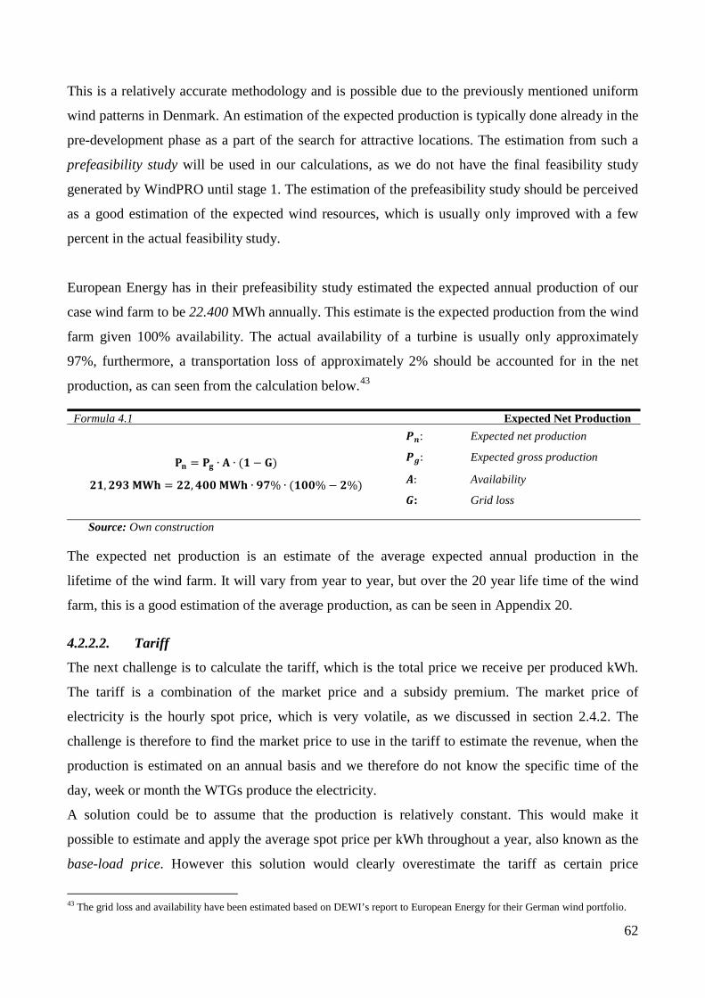
62

This is a relatively accurate methodology and is possible due to the previously mentioned uniform

wind patterns in Denmark. An estimation of the expected production is typically done already in the

pre-development phase as a part of the search for attractive locations. The estimation from such a

prefeasibility study will be used in our calculations, as we do not have the final feasibility study

generated by WindPRO until stage 1. The estimation of the prefeasibility study should be perceived

as a good estimation of the expected wind resources, which is usually only improved with a few

percent in the actual feasibility study.

European Energy has in their prefeasibility study estimated the expected annual production of our

case wind farm to be 22.400 MWh annually. This estimate is the expected production from the wind

farm given 100% availability. The actual availability of a turbine is usually only approximately

97%, furthermore, a transportation loss of approximately 2% should be accounted for in the net

production, as can seen from the calculation below.43

Formula 4.1 Expected Net Production

𝐏𝐧 = 𝐏𝐠 ∙ 𝐀 ∙ (𝟏 − 𝐆)

𝟐𝟏,𝟐𝟗𝟑 𝐌𝐖𝐡 = 𝟐𝟐,𝟒𝟎𝟎 𝐌𝐖𝐡 ∙ 𝟗𝟕% ∙ (𝟏𝟎𝟎% − 𝟐%)

𝑷𝒏: Expected net production

𝑷𝒈: Expected gross production

𝑨: Availability

𝑮: Grid loss


The expected net production is an estimate of the average expected annual production in the

lifetime of the wind farm. It will vary from year to year, but over the 20 year life time of the wind

farm, this is a good estimation of the average production, as can be seen in Appendix 20.

4.2.2.2. Tariff

The next challenge is to calculate the tariff, which is the total price we receive per produced kWh.

The tariff is a combination of the market price and a subsidy premium. The market price of

electricity is the hourly spot price, which is very volatile, as we discussed in section 2.4.2. The

challenge is therefore to find the market price to use in the tariff to estimate the revenue, when the

production is estimated on an annual basis and we therefore do not know the specific time of the

day, week or month the WTGs produce the electricity.

A solution could be to assume that the production is relatively constant. This would make it

possible to estimate and apply the average spot price per kWh throughout a year, also known as the

base-load price. However this solution would clearly overestimate the tariff as certain price

43 The grid loss and availability have been estimated based on DEWI’s report to European Energy for their German wind portfolio.

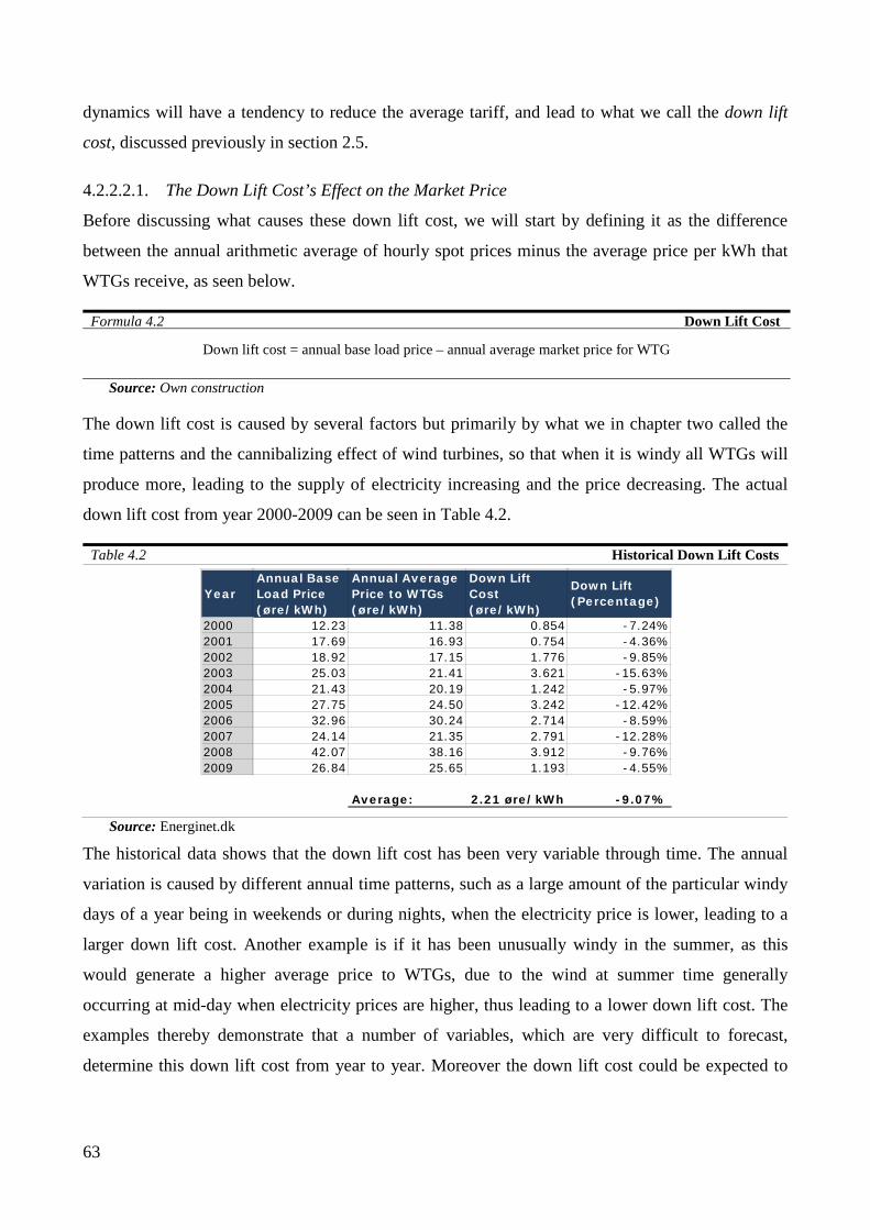
63

dynamics will have a tendency to reduce the average tariff, and lead to what we call the down lift

cost, discussed previously in section 2.5.

4.2.2.2.1. The Down Lift Cost’s Effect on the Market Price

Before discussing what causes these down lift cost, we will start by defining it as the difference

between the annual arithmetic average of hourly spot prices minus the average price per kWh that

WTGs receive, as seen below.

Formula 4.2 Down Lift Cost

Down lift cost = annual base load price – annual average market price for WTG


The down lift cost is caused by several factors but primarily by what we in chapter two called the

time patterns and the cannibalizing effect of wind turbines, so that when it is windy all WTGs will

produce more, leading to the supply of electricity increasing and the price decreasing. The actual

down lift cost from year 2000-2009 can be seen in Table 4.2.

Table 4.2 Historical Down Lift Costs

Source: Energinet.dk

The historical data shows that the down lift cost has been very variable through time. The annual

variation is caused by different annual time patterns, such as a large amount of the particular windy

days of a year being in weekends or during nights, when the electricity price is lower, leading to a

larger down lift cost. Another example is if it has been unusually windy in the summer, as this

would generate a higher average price to WTGs, due to the wind at summer time generally

occurring at mid-day when electricity prices are higher, thus leading to a lower down lift cost. The

examples thereby demonstrate that a number of variables, which are very difficult to forecast,

determine this down lift cost from year to year. Moreover the down lift cost could be expected to

YearAnnual Base Load Price (øre/kWh)

Annual Average Price to WTGs (øre/kWh)

Down Lift Cost (øre/kWh)

Down Lift (Percentage)

2000 12.23 11.38 0.854 -7.24%2001 17.69 16.93 0.754 -4.36%2002 18.92 17.15 1.776 -9.85%2003 25.03 21.41 3.621 -15.63%2004 21.43 20.19 1.242 -5.97%2005 27.75 24.50 3.242 -12.42%2006 32.96 30.24 2.714 -8.59%2007 24.14 21.35 2.791 -12.28%2008 42.07 38.16 3.912 -9.76%2009 26.84 25.65 1.193 -4.55%

Average: 2.21 øre/kWh -9.07%

64

change during the next three years due to a number of factors, such as the previously mentioned

cable between DK East and DK West or more WTGs being installed.

4.2.2.2.2. Estimating the Market Price that Wind Farms Receive

Due to the complex nature of the down lift cost we have (as non-experts) decided to use the

expectations from the market as a best estimate. This can be done by using the forward that the

WTG administrator Vindenergi Danmark offers in collaboration with the energy trader Nordjysk

Elhandel. This is a service whereby WTG owners can fix their market price on electricity for one

year at a time, up to three years in advance. The forward is created based on the forwards traded on

Nord Pool. It consists of a 1-year base-load contract plus a 1-year CfD minus the down lift cost. The

contract for 2013 traded primo 2010 at 34.32 øre/kWh.44 This price is 4.5 øre/kWh lower than the

base load contract trading on Nord Pool, so the down lift cost is estimated by Vindenergi Danmark

to be 4.5 øre/kwh in 2013. This is significantly higher than the 1.19 øre it has been in year 2009 as

can be seen in Table 4.2. This could indicate that Vindenergi Danmark charges a significant risk

premium to offer the service, and/or that the down lift cost is expected to increase significantly in

the future. However, we consider it to be the best estimate of the actual market price that a wind

farm can expect to receive in year 2013 – we will therefore use it in our DCF calculation.

4.2.2.2.3. Subsidy Premium

In addition to the market price, the WTG owner has the right to receive subsidies on the production.

From February 2008, all new turbines receive an additional 25 øre/kWh for the first 22,000 full load

hours, which approximates the entire production in the first 10 years. 45 In our case, with 3 Siemens

2.3 MW turbines, the subsidies will be rewarded for the first 151,800 MWh. The subsidies are fixed

from the day the turbines deliver the first kWh to the grid, i.e. any change in subsidies that occur

after this point in time will not have any influence on the turbine.

4.2.2.3. Costs

A WTG has six significant operating costs as can be seen in Table 4.3. The combination of the

insurance, service and technical management, creates a total insurance for the wind turbine owner

against any kind of unexpected costs in the 20 years expected lifetime of the windmill. Further costs

are land lease, administration fees and own power consumption. The latter cost is due to the WTG

consuming electricity, when positioning itself optimally in the wind.

44 The price is the closing price of the forward the 4th of January 2010. This date is chosen despite our cut-off date, as the particular forward was not traded the 30th of December 2009. 45 In our case this equals: 2.3 MW . 3 turbines . 22,000 full load hours = 151,800 MWh.

65

Out of the six costs two are variable: the technical management and the land lease. The costs have

been estimated based on data from EE, an external wind farm prospect and dkvind, which can be

seen in Appendix 9.

Table 4.3 Annual Cost for One Siemens 2.3 MW WTG

Expense: Annual costs 2009 Annual Costs 2013

Service (from year 3)46 204,300 DKK 216,805 DKK

Technical management 0.080 DKK/kWh 0.0849 DKK./kWh

Insurance: 150,000 DKK 159,181 DKK

Land lease: 4% of revenue 4% of revenue ≈ 170,000 DKK/Year

Administration: 90,000 DKK 95,509 DKK

Own energy consumption: 30,000 DKK 31,836 DKK

Source: Estimations made from European Energy, Vognkær Ny Møllelaug and dkvind, see Appendix 9.

4.2.2.4. The Depreciation Effect on Tax

Fixed capital investments depreciate in value throughout their operational life. This is

acknowledged by the Danish tax laws, which make it possible to depreciate this value decrease. The

Danish corporate tax is today 25%, and wind turbines can be depreciated in accordance with the

accelerated depreciation principle by up to 25% of the remaining book value each year (Grant

Thornton 2008). Any remaining book value is depreciated in the last operational year of the

turbine.47 Furthermore, these depreciation tax shields can be carried forward. This means that if

you cannot use your tax shield in a given year due to insufficient profit, the tax shield can be carried

forward until it can be utilized. This is the case in our project, where the tax shields in the first years

are so large compared to profits that they cannot be fully utilized and therefore are carried forward.

4.2.2.5. Investments in Fixed Assets and Working Capital

A wind farm generally has one investment in fixed assets, namely the purchase and installation of

the WTGs. Any investments in spare parts are included in the service and insurance agreements,

and will therefore not have any impact on the FCF in the operational phase. A wind farm does not

have any significant change in working capital either, and are therefore not included in the FCF.

46 Siemens provides a two year warranty on new turbines, thus no service contract is needed for the first two years. 47 In Danish: “udgiftsført”.

66

4.2.2.6. The Free Cash Flow

Having discussed all the inputs, we can now set up the free

cash flows for the operational wind farm, from year 2013-

2032. A preview of one FCF can be seen in the table to the

right, and the entire cash flow can be seen in Appendix 18.

Having found the free cash flow, we are now ready to step

two of the DCF model, estimating the cost of equity.

4.2.3. Step 2: Estimating the Cost of Equity We now turn to the other variable in the standard DCF model in Formula 3.1, the discount rate for

the operational phase, which in our case is the cost of equity as we do not consider debt financing

until chapter 5. The cost of equity can be found using CAPM, introduced in Formula 3.2. The

CAPM estimates the cost of equity from three inputs, risk-free rate, risk premium and beta. Out of

these three, only the beta is company-specific, whereas the others are general for the market.

Despite the CAPM being a simple formula with only three variables, the actual use is difficult, and

estimating the “correct” market risk premium and beta are considered among the most debated

topics in finance (Koller et al. 2005: 105). It could also be argued that a liquidity premium should

be added to the cost of equity reflecting the fact that wind farms are not traded on efficient markets.

However, this easily becomes a fudge factor, and also seems inconsistent in relation to our

assumption of market completeness, and it will therefore not be included.

4.2.3.1. The Market Risk Premium

The market risk premium is defined as the difference between the return on the market portfolio and

the risk-free rate of return. Although being simple to define, much disagreement exists with regard

to actual estimation, where many practitioners prefer estimates based on forward looking data (ex-

ante method), academics often use the historical data due to a much larger dataset being available

(ex-post method).48 But even within the ex-post methods, disagreements exist, which makes it clear

that estimating the premium is no exact science.49 In Table 4.4 below, a comparison of a number of

risk premium estimates for the Danish market are presented.

48 FSR 2002: 60. 49 The disagreement about market risk premiums is clear from the study published in 2008 by Fernández, which surveys the market risk premium used by 1,400 finance professors

Free Cash Flow Year 20131. Revenue 12,631,269 2. Cost -3,172,571 3. EBITDA 9,458,698

4. Depreciation -15,250,000

5. EBIT -5,791,302

6. Tax -

7. Profit after tax -5,791,302

8. Investments in fixed assets -

9. Investments in working capital -

10. Free Cash Flow 9,458,698

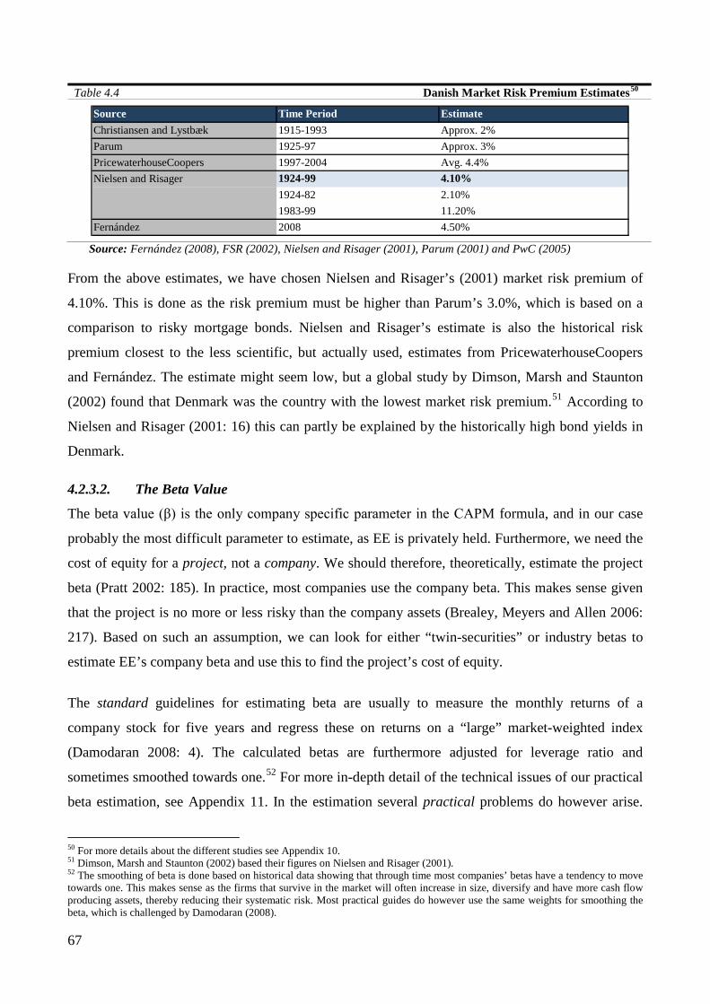
67

Table 4.4 Danish Market Risk Premium Estimates50

Source: Fernández (2008), FSR (2002), Nielsen and Risager (2001), Parum (2001) and PwC (2005)

From the above estimates, we have chosen Nielsen and Risager’s (2001) market risk premium of

4.10%. This is done as the risk premium must be higher than Parum’s 3.0%, which is based on a

comparison to risky mortgage bonds. Nielsen and Risager’s estimate is also the historical risk

premium closest to the less scientific, but actually used, estimates from PricewaterhouseCoopers

and Fernández. The estimate might seem low, but a global study by Dimson, Marsh and Staunton

(2002) found that Denmark was the country with the lowest market risk premium.51 According to

Nielsen and Risager (2001: 16) this can partly be explained by the historically high bond yields in

Denmark.

4.2.3.2. The Beta Value

The beta value (β) is the only company specific parameter in the CAPM formula, and in our case

probably the most difficult parameter to estimate, as EE is privately held. Furthermore, we need the

cost of equity for a project, not a company. We should therefore, theoretically, estimate the project

beta (Pratt 2002: 185). In practice, most companies use the company beta. This makes sense given

that the project is no more or less risky than the company assets (Brealey, Meyers and Allen 2006:

217). Based on such an assumption, we can look for either “twin-securities” or industry betas to

estimate EE’s company beta and use this to find the project’s cost of equity.

The standard guidelines for estimating beta are usually to measure the monthly returns of a

company stock for five years and regress these on returns on a “large” market-weighted index

(Damodaran 2008: 4). The calculated betas are furthermore adjusted for leverage ratio and

sometimes smoothed towards one.52 For more in-depth detail of the technical issues of our practical

beta estimation, see Appendix 11. In the estimation several practical problems do however arise.

50 For more details about the different studies see Appendix 10. 51 Dimson, Marsh and Staunton (2002) based their figures on Nielsen and Risager (2001). 52 The smoothing of beta is done based on historical data showing that through time most companies’ betas have a tendency to move towards one. This makes sense as the firms that survive in the market will often increase in size, diversify and have more cash flow producing assets, thereby reducing their systematic risk. Most practical guides do however use the same weights for smoothing the beta, which is challenged by Damodaran (2008).

Source Time Period EstimateChristiansen and Lystbæk 1915-1993 Approx. 2%Parum 1925-97 Approx. 3%PricewaterhouseCoopers 1997-2004 Avg. 4.4%Nielsen and Risager 1924-99 4.10%

1924-82 2.10%1983-99 11.20%

Fernández 2008 4.50%

68

First of all, it is not clear how many peer companies are needed. Generally the rule seems to be “as

many as possible”. In addition it is unclear how much the peers need to resemble the company to be

“fair” estimates. In our case, finding just a few companies that resemble EE is difficult, as very few

renewable energy IPPs are listed.53 But we have identified three peers, which in many ways

resemble EE in size, markets active and business model etc. The three companies are Greentech

Energy Systems, Alerion Clean Power and Theolia.54 While the companies on the surface resemble

EE, they are problematic as peers. All have within the last faced either serious liquidity issues,

refocusing of their business strategy, or new significant joint ventures. This has created some large

fluctuations in their stock prices making any beta estimation very “noisy”. Despite this, we have

calculated the betas based on the above instructions. However, they have not been smoothed due to

comparison reasons to the industry betas presented later. As a “sanity check” we have included the

world largest wind farm owner Iberdrola Renovables, but since their stock did not start trading until

December 2007, we have calculated the beta on weekly data. The betas are presented below.

Table 4.5 Beta Analysis of Peer Companies55

Source: Datastream

The beta values marked with blue in Table 4.5 are the best estimates of the unlevered betas in our

opinion. It is important to be very cautious when interpreting the figures, due to the complications

mentioned above. The uncertainty of beta estimations is clear from large standard errors in the

table. To get a 95% confidence interval of our beta estimation, we should add and subtract 2

standard errors in each end of the estimates. In the case of Alerion the (levered) beta is thus between

0.29 and 1.17 – hardly a tight range. The reason that we present two different unlevered betas is due

53 Emerging Energy Research tracks 19 renewable energy IPPs active in Europe of which only 6 are independently quoted companies and many of them also hold a large portfolio of conventional generation assets (Emerging Energy Research 2009b: 4-8). 54 More company specific information can be found in Appendix 11. 55 For more details on the beta estimation please see Appendix 12 and the dataset used for the calculation on the enclosed CD. It should be noted that beta values have been calculated from 2003-2008, since debt-equity ratios were not available for 2009, at the time of the analysis.

Monthly Weekly Monthly WeeklyBeta 0.73 0.49 Beta 0.92

Unlevered (2008) 0.37 0.25 Unlevered (2008) 0.87Unlevered (Average) 0.54 0.29 Unlevered (Average) 0.87

R-squared 0.15 0.14 R-squared 0.42Standard Error 0.22 0.12 Standard Error 0.11

Monthly Weekly Monthly WeeklyBeta 1.66 1.56 Beta 1.64 0.67

Unlevered (2008) 0.46 0.44 Unlevered (2008) 1.29 0.53Unlevered (Average) 0.62 0.58 Unlevered (Average) 1.06 0.44

R-squared 0.14 0.30 R-squared 0.23 0.05Standard Error 0.54 0.24 Standard Error 0.40 0.28

Alerion Iberdrola Renovables

Theolia Greentech

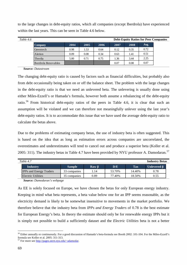
69

to the large changes in debt-equity ratios, which all companies (except Iberdrola) have experienced

within the last years. This can be seen in Table 4.6 below.

Table 4.6 Debt-Equity Ratios for Peer Companies

Source: Datastream

The changing debt-equity ratio is caused by factors such as financial difficulties, but probably also

from debt occasionally being taken on or off the balance sheet. The problem with the large changes

in the debt-equity ratio is that we need an unlevered beta. The unlevering is usually done using

either Miles-Ezzell’s or Hamada’s formula, however both assume a rebalancing of the debt-equity

ratio.56 From historical debt-equity ratios of the peers in Table 4.6, it is clear that such an

assumption will be violated and we can therefore not meaningfully unlever using the last year’s

debt-equity ratios. It is to accommodate this issue that we have used the average debt-equity ratio to

calculate the betas above.

Due to the problems of estimating company betas, the use of industry beta is often suggested. This

is based on the idea that as long as estimation errors across companies are uncorrelated, the

overestimates and underestimates will tend to cancel out and produce a superior beta (Koller et al.

2005: 311). The industry betas in Table 4.7 have been provided by NYU professor A. Damodaran.57

Table 4.7 Industry Betas

Source: Damodaran’s webpage

As EE is solely focused on Europe, we have chosen the betas for only European energy industry.

Keeping in mind what beta represents, a beta value below one for an IPP seems reasonable, as the

electricity demand is likely to be somewhat insensitive to movements in the market portfolio. We

therefore believe that the industry beta from IPPs and Energy Traders of 0.78 is the best estimate

for European Energy’s beta. In theory the estimate should only be for renewable energy IPPs but it

is simply not possible to build a sufficiently dataset and the Electric Utilities beta is not a better

56 Either annually or continuously. For a good discussion of Hamada’s beta-formula see Booth 2002: 101-104. For the Miles-Ezzell’s formula see Koller et al. 2005: 311-313. 57 For more see http://pages.stern.nyu.edu/~adamodar.

Company 2004 2005 2006 2007 2008 Avg.

Greentech 0.98 1.53 0.64 0.12 0.35 0.72Alerion 0.09 0.08 0.34 0.63 1.41 0.51Theolia 5.00 0.71 0.75 1.36 3.44 2.25Iberdrola Renovables 0.07 0.08 0.07

Industry Sample Raw β D/E Tax Unlevered β IPPs and Energy Traders 33 companies 1.14 53.70% 14.40% 0.78Electric Utilities 35 companies 0.89 77.40% 18.50% 0.55

http://pages.stern.nyu.edu/~adamodar

70

alternative. The industry beta estimate is also relatively close to what is probably the best peer

estimate namely the beta of Iberdrola and surprisingly the average of the four “recommended” betas

is actually 0.77.

It should be noted that Damodaran’s betas by no means are “perfect”, but they provide a good

estimate based on the above reasoning. One problem is that Damodaran uses the Hamada-formula

to unlever his betas. Furthermore the betas are based on stock returns measured against local market

indexes, something often seen in practice but theoretically incorrect, as local market indexes often

are heavily weighted towards one industry. This means that the beta does not represent the

sensitivity to the market portfolio, but instead towards some specific industries (Koller et al. 2005:

310).

4.2.3.3. The Risk-free Rate of Return

The risk-free rate of return is defined as the return on an asset that has no covariance with the

market, and (in theory) a zero beta portfolio should be constructed to estimate it. In practice, long

term government default-free bonds are used. Another theoretical ideal that is broken is that, in

theory, the cash flows should be discounted with a risk-free rate of a matching maturity. In practice,

a 10-year bond is recommended (Koller et al. 2005: 296). According to annual surveys from 1998

to 2004 by PricewaterhouseCoopers, the majority of Danish corporate finance companies use a 10-

year Danish government bond to estimate the risk-free rate (PwC 2005). We have chosen to do the

same and have therefore used these to estimate the risk-free rate. This bond has an effective interest

rate of 3.62%.58 In order to ensure consistency we have chosen a Danish bond, so the risk-free rate

and cash flows are denominated in the same currency. Having found the last necessary input for the

CAPM-formula we will now calculate our cost of equity.

4.2.3.4. The Cost of Equity

We will now estimate the unlevered cost of equity applying the unlevered beta of 0.78, a risk-free

rate of 3.62 % and a market risk premium of 4.10 % in the CAPM formula, as seen below.

Formula 4.3 Calculation of Cost of Equity

𝐄(𝐑𝐢) = 𝐫𝐟 + 𝛃𝐢(𝐄(𝐑𝐦) − 𝐫𝐟)

𝟎.𝟎𝟔𝟖𝟐 = 𝟎.𝟎𝟑𝟔𝟐 + 𝟎.𝟕𝟖(𝟎.𝟎𝟒𝟏)

𝑬(𝑹𝒊): Expected return on asset 6.82%

𝒓𝒇: Risk-free rate = 3.62%

𝜷𝒊: Beta on asset = 0.78

𝑹𝒎: Market risk premium = 4.1%


58 From the home page of Danmarks Nationalbank, 30th of December 2009.

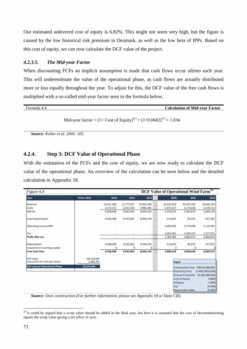
71

Our estimated unlevered cost of equity is 6.82%. This might not seem very high, but the figure is

caused by the low historical risk premium in Denmark, as well as the low beta of IPPs. Based on

this cost of equity, we can now calculate the DCF value of the project.

4.2.3.5. The Mid-year Factor

When discounting FCFs an implicit assumption is made that cash flows occur ultimo each year.

This will underestimate the value of the operational phase, as cash flows are actually distributed

more or less equally throughout the year. To adjust for this, the DCF value of the free cash flows is

multiplied with a so-called mid-year factor seen in the formula below.

Formula 4.4 Calculation of Mid-year Factor

Mid-year factor = (1+ Cost of Equity)0.5 = (1+0.0682)0.5 = 1.034

Source: Koller et al. 2005: 105.

4.2.4. Step 3: DCF Value of Operational Phase With the estimation of the FCFs and the cost of equity, we are now ready to calculate the DCF

value of the operational phase. An overview of the calculation can be seen below and the detailed

calculation in Appendix 18.

Figure 4.4 DCF Value of Operational Wind Farm59

Source: Own construction (For further information, please see Appendix 18 or Data CD).

59 It could be argued that a scrap value should be added in the final year, but here it is assumed that the cost of decommissioning equals the scrap value giving a net effect of zero.

Year Primo 2013 2013 2014 2015 2030 2031 2032

Revenue 12,631,269 12,777,427 12,926,508 … 10,232,836 10,437,493 10,646,243 Costs 3,172,571 3,231,763 3,982,365 … 5,073,157 5,174,620 5,278,113 EBITDA 9,458,698 9,545,663 8,944,143 ... 5,159,679 5,262,873 5,368,130

Asset Depreciation -9,458,698 -9,545,663 -8,944,143 ... -114,633 -85,975 -257,925

Operating income/EBIT - - - ... 5,045,046 5,176,898 5,110,205

Tax - - - … 1,261,261 1,294,224 1,277,551 Profit after tax - - - … 3,783,784 3,882,673 3,832,654

Depreciation 9,458,698 9,545,663 8,944,143 … 114,633 85,975 257,925 Investment in working capital 0 0 0 … 0 0 0Free Cash Flow 9,458,698 9,545,663 8,944,143 … 3,898,418 3,968,648 4,090,579

DCF value 68,193,605Correction for mid-year factor 2,286,391

DCF valueof Operational Phase 70,479,996

Input:

Construction Cost 61,000,000DKK Electricity Price 0.3432 DKK/kWhAnnual Production 21,293,440 kWhCost of Equity 6.82%Inflation 2.00%Tax 25.00%Depreciation Rate 25.00%

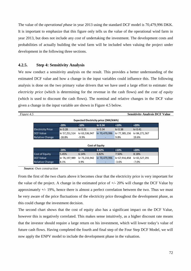
72

The value of the operational phase in year 2013 using the standard DCF model is 70,479,996 DKK.

It is important to emphasize that this figure only tells us the value of the operational wind farm in

year 2013, but does not include any cost of undertaking the investment. The development costs and

probabilities of actually building the wind farm will be included when valuing the project under

development in the following three sections.

4.2.5. Step 4: Sensitivity Analysis We now conduct a sensitivity analysis on the result. This provides a better understanding of the

estimated DCF value and how a change in the input variables could influence this. The following

analysis is done on the two primary value drivers that we have used a large effort to estimate: the

electricity price (which is determining for the revenue in the cash flows) and the cost of equity

(which is used to discount the cash flows). The nominal and relative changes in the DCF value

given a change in the input variable are shown in Figure 4.5 below.

Figure 4.5 Sensitivity Analysis DCF Value


From the first of the two charts above it becomes clear that the electricity price is very important for

the value of the project. A change in the estimated price of +/- 20% will change the DCF Value by

approximately +/- 19%, hence there is almost a perfect correlation between the two. Thus we must

be very aware of the price fluctuations of the electricity price throughout the development phase, as

this could change the investment decision.

The second chart shows that the cost of equity also has a significant impact on the DCF Value,

however this is negatively correlated. This makes sense intuitively, as a higher discount rate means

that the investor should require a large return on his investment, which will lower today’s value of

future cash flows. Having completed the fourth and final step of the Four Step DCF Model, we will

now apply the ENPV model to include the development phase in the valuation.

-20% -10% kr 0.34 +10% +20%Electricity Price kr 0.28 kr 0.31 kr 0.34 kr 0.38 kr 0.41DCF Value kr 57,251,514 kr 63,536,947 kr 70,479,996 kr 77,385,156 kr 84,271,567Relative Change -18.8% -9.9% - 9.8% 19.6%

-20% -10% 6.82% +10% +20%Cost of Equity 5.45% 6.14% 6.82% 7.50% 8.18%DCF Value kr 76,197,989 kr 73,233,942 kr 70,479,996 kr 67,916,858 kr 65,527,291Relative Change 8.1% 3.9% - -3.6% -7.0%

Cost of Equity

Expected Electricity price (DKK/kWh)

73

4.3 Expected Net Present Value Having estimated the value of the operational phase, we are now ready to estimate the value of a

wind farm under development. This is done by introducing the event that the wind farm fails during

the development phase using the ENPV model. This DCF based technique is, however, not able to

handle the market uncertainty and decisions in the development phase – thereby underestimating

the value of the project.

4.3.1. Introduction In chapter 3, two DCF based models were discussed to value a wind farm under development, the

ENPV model and DTA. Of these two models we have chosen to apply ENPV, as it is not possible

to estimate the discount rate needed in the DTA correctly. The below figure gives illustrates how

ENPV values a wind farm under development.

Figure 4.6 Illustration of the Events During the Development Phase


As Figure 4.5 indicates, each stage can turn out as either a success or a failure, caused by events in

the development phase. If the project succeeds, it moves into the next stage, and ultimately, the

wind farm is constructed, with EE receiving the value of the operational wind farm. If it fails, the

project has received a denial from the city council or the compensation demands have become too

large. A failure thus implies that the value of the project will decrease to zero. The ENPV then

Operational PhaseDevelopment Phase

Operational Cash Flow

Primo 2010

Ultimo 2012

Ultimo 2032


Stage 2 VVM and Final

Approval


Stage 4Construction

74

weights each possible outcome with the probabilities found in Figure 2.2 in chapter 2, and discounts

these values in order to find the present value of the wind farm under development.

4.3.2. The Probabilities of Events It is important to note that the probabilities represent either success or failure events in the

development phase, as it assumed that market developments have no influence. This means that the

probabilities reflect the possibility of failing in the development phase due to technical issues or a

political rejection of the project. A similar approach is found in Méndez et al. (2009: 3-4).

4.3.2.1. Non-Measurable versus Measurable Probabilities

A distinction between non-measurable and measurable probabilities is important, as it has been

stated that the probabilities used in the ENPV model reflect the events in the development stages.

But probabilities such as the entire subsidy system changing or a new generation technology being

invented, are not accounted for in the probabilities. This is due to the fact that the probabilities of

such events cannot be measured meaningfully. In general, probabilities which cannot be foreseen at

the time of the initial investment decision should not be included when performing a valuation

(Willigers and Hansen 2008: 524).

4.3.3. The Discount Rate A great advantage of the ENPV model is that it explicitly separates the development and

operational phase. The separation leads to a discussion of which cost of capital to use for

discounting in each phase. As argued in section 3.4, if the notion that the probability of an event is

uncorrelated to the market is accepted, then the risk-free rate should be used to discount the costs of

development. Meanwhile, the cash flows of the operational phase should be discounted at the cost

of equity, as these will still be subject to market risk. The idea to let the events be uncorrelated with

the market is to avoid the problems of estimating the discount rate, as discussed in DTA.

4.3.4. Calculation of Expected Net Present Value The ENPV of the wind farm under development is calculated from the probabilities and costs that

were estimated in chapter 2, and the value of the operational phase estimated in section 4.2.4. The

calculations are shown in Figure 4.7.

75

Figure 4.7 ENPV Calculation


All payments for the stages are assumed to occur in the beginning of each stage, whereas the

outcome is resolved at the end. As an example, EE would decide to invest 500,000 in a VVM report

without knowing if the final approval would be granted until 12 month later. The chance of entering

stage 2 leading to an investment of 500,000 is 50%, as there is 50% chance that stage 1 succeeds.

The chance of entering stage 3 (complaints and compensation), leading to an investment of an

additional 500,000 is thus 25%, because both of the prior stages have a 50% chance of succeeding.

In the last column of Figure 4.7, the probability weighted PVs of each stage have been found. The

four development stages have been discounted with the risk-free rate, whereas the value of the

operational phase has been discounted with the cost of equity. The total value of this column is

DKK -60,879, which is the expected net present value of the wind farm under development when

events are taken into consideration. A negative expected net present value indicates that the project

does not yield the return on equity that EE should require for this project, and their money would be

better spent elsewhere.

4.3.4.1. Sensitivity Analysis

To understand the result better, we now perform a sensitivity analysis of the ENPV, shown in

Figure 4.8 below. Here we test the sensitivity to the probabilities of events, which we introduced

with the ENPV. There are two reasons why we test the probabilities. First, they determine whether

the wind farm is developed, and therefore have a large influence on the ENPV of the project.

Second, the probabilities have been estimated for an average wind farm, and it is therefore relevant

to see what the value would be with other probabilities. The sensitivity analysis has only been

performed on stage 1-3, as stage 4 has a 100% probability of succeeding.

Stage Time Prob. Stage

Probability of Construction Cash Flow (t) PV (t=0) Probability

Weighted PVStage 1: Analysis and Pre-approval 0 50% 100% -100,000 -100,000 -100,000 Stage 2: VVM & Final Approval 0.5 50% 50% -500,000 -491,189 -245,594 Stage 3: Complaints and Compensation 1.5 80% 25% -500,000 -474,029 -118,507 Stage 4: Construction 2.5 100% 20% -61,000,000 -55,811,136 -11,162,227 Value of Operational Phase 3 - 20% 70,479,996 57,827,251 11,565,450

ENPV -60,879

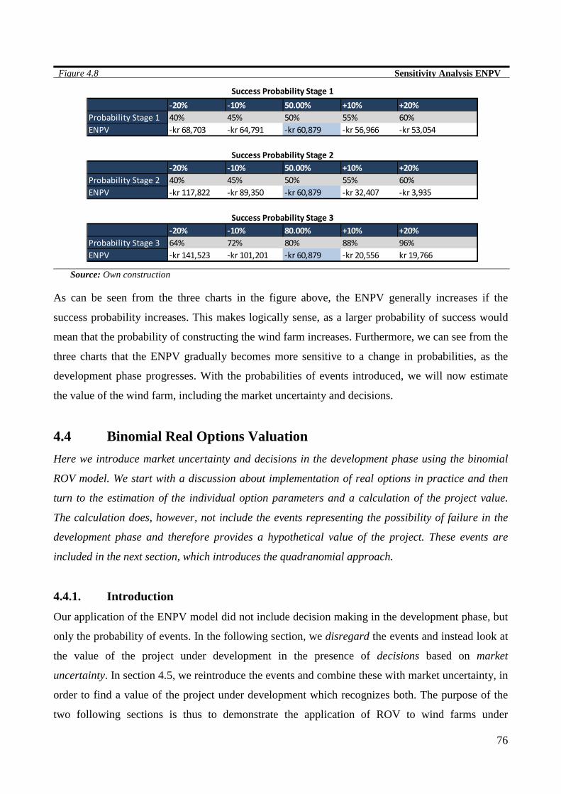
76

Figure 4.8 Sensitivity Analysis ENPV


As can be seen from the three charts in the figure above, the ENPV generally increases if the

success probability increases. This makes logically sense, as a larger probability of success would

mean that the probability of constructing the wind farm increases. Furthermore, we can see from the

three charts that the ENPV gradually becomes more sensitive to a change in probabilities, as the

development phase progresses. With the probabilities of events introduced, we will now estimate

the value of the wind farm, including the market uncertainty and decisions.

4.4 Binomial Real Options Valuation Here we introduce market uncertainty and decisions in the development phase using the binomial

ROV model. We start with a discussion about implementation of real options in practice and then

turn to the estimation of the individual option parameters and a calculation of the project value.

The calculation does, however, not include the events representing the possibility of failure in the

development phase and therefore provides a hypothetical value of the project. These events are

included in the next section, which introduces the quadranomial approach.

4.4.1. Introduction Our application of the ENPV model did not include decision making in the development phase, but

only the probability of events. In the following section, we disregard the events and instead look at

the value of the project under development in the presence of decisions based on market

uncertainty. In section 4.5, we reintroduce the events and combine these with market uncertainty, in

order to find a value of the project under development which recognizes both. The purpose of the

two following sections is thus to demonstrate the application of ROV to wind farms under

-20% -10% 50.00% +10% +20%Probability Stage 1 40% 45% 50% 55% 60%ENPV -kr 68,703 -kr 64,791 -kr 60,879 -kr 56,966 -kr 53,054

-20% -10% 50.00% +10% +20%Probability Stage 2 40% 45% 50% 55% 60%ENPV -kr 117,822 -kr 89,350 -kr 60,879 -kr 32,407 -kr 3,935

-20% -10% 80.00% +10% +20%Probability Stage 3 64% 72% 80% 88% 96%ENPV -kr 141,523 -kr 101,201 -kr 60,879 -kr 20,556 kr 19,766

Success Probability Stage 1



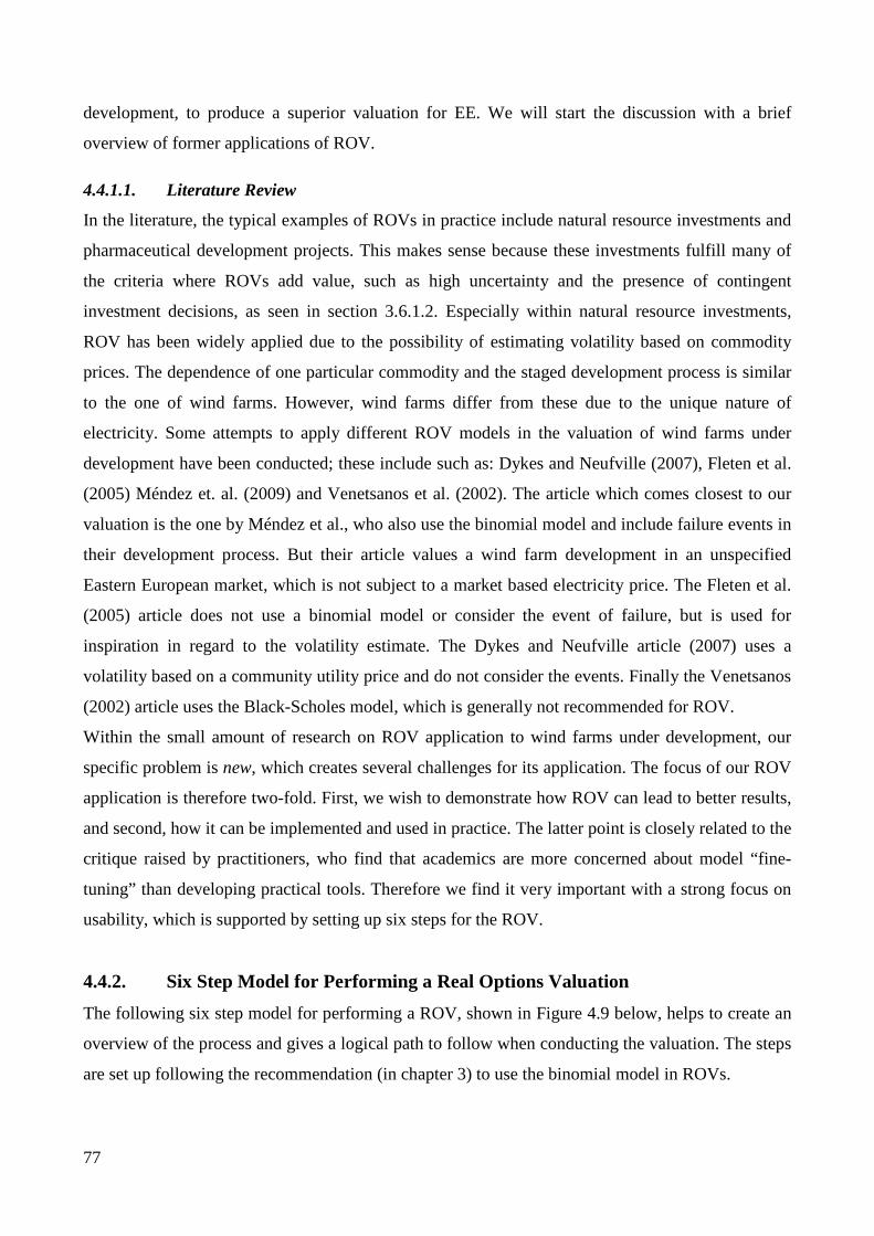
77

development, to produce a superior valuation for EE. We will start the discussion with a brief

overview of former applications of ROV.

4.4.1.1. Literature Review

In the literature, the typical examples of ROVs in practice include natural resource investments and

pharmaceutical development projects. This makes sense because these investments fulfill many of

the criteria where ROVs add value, such as high uncertainty and the presence of contingent

investment decisions, as seen in section 3.6.1.2. Especially within natural resource investments,

ROV has been widely applied due to the possibility of estimating volatility based on commodity

prices. The dependence of one particular commodity and the staged development process is similar

to the one of wind farms. However, wind farms differ from these due to the unique nature of

electricity. Some attempts to apply different ROV models in the valuation of wind farms under

development have been conducted; these include such as: Dykes and Neufville (2007), Fleten et al.

(2005) Méndez et. al. (2009) and Venetsanos et al. (2002). The article which comes closest to our

valuation is the one by Méndez et al., who also use the binomial model and include failure events in

their development process. But their article values a wind farm development in an unspecified

Eastern European market, which is not subject to a market based electricity price. The Fleten et al.

(2005) article does not use a binomial model or consider the event of failure, but is used for

inspiration in regard to the volatility estimate. The Dykes and Neufville article (2007) uses a

volatility based on a community utility price and do not consider the events. Finally the Venetsanos

(2002) article uses the Black-Scholes model, which is generally not recommended for ROV.

Within the small amount of research on ROV application to wind farms under development, our

specific problem is new, which creates several challenges for its application. The focus of our ROV

application is therefore two-fold. First, we wish to demonstrate how ROV can lead to better results,

and second, how it can be implemented and used in practice. The latter point is closely related to the

critique raised by practitioners, who find that academics are more concerned about model “fine-

tuning” than developing practical tools. Therefore we find it very important with a strong focus on

usability, which is supported by setting up six steps for the ROV.

4.4.2. Six Step Model for Performing a Real Options Valuation The following six step model for performing a ROV, shown in Figure 4.9 below, helps to create an

overview of the process and gives a logical path to follow when conducting the valuation. The steps

are set up following the recommendation (in chapter 3) to use the binomial model in ROVs.

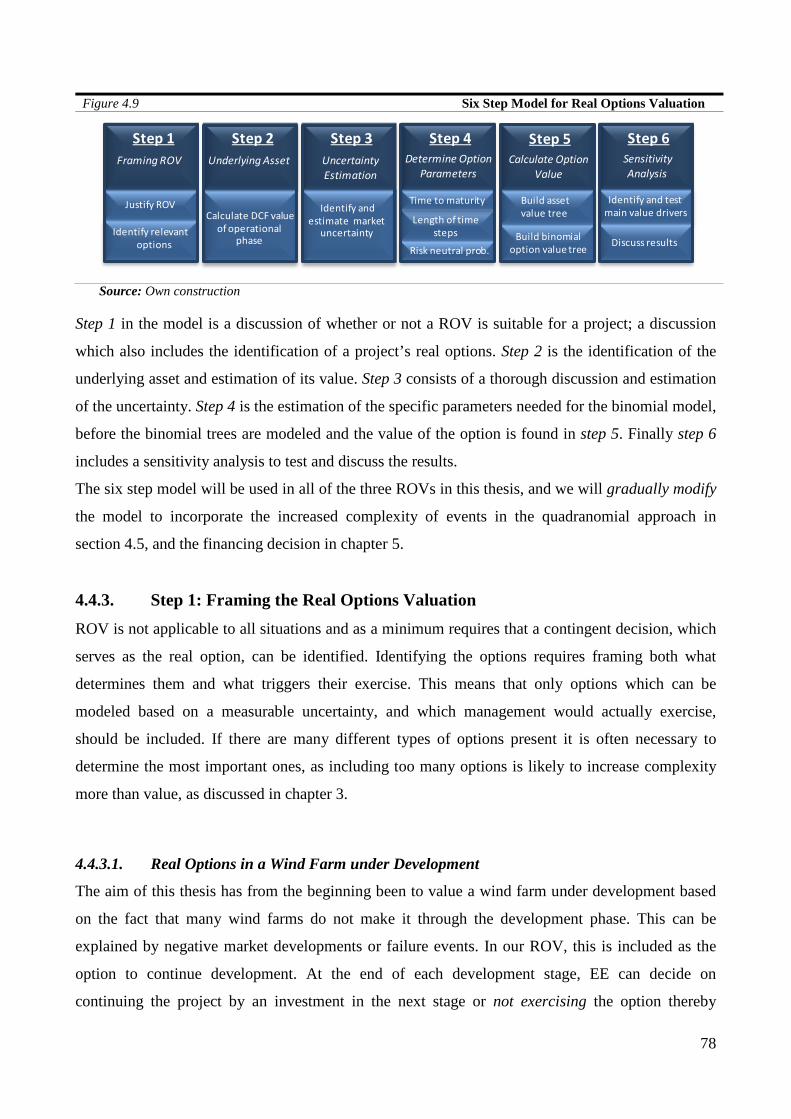
78

Figure 4.9 Six Step Model for Real Options Valuation


Step 1 in the model is a discussion of whether or not a ROV is suitable for a project; a discussion

which also includes the identification of a project’s real options. Step 2 is the identification of the

underlying asset and estimation of its value. Step 3 consists of a thorough discussion and estimation

of the uncertainty. Step 4 is the estimation of the specific parameters needed for the binomial model,

before the binomial trees are modeled and the value of the option is found in step 5. Finally step 6

includes a sensitivity analysis to test and discuss the results.

The six step model will be used in all of the three ROVs in this thesis, and we will gradually modify

the model to incorporate the increased complexity of events in the quadranomial approach in

section 4.5, and the financing decision in chapter 5.

4.4.3. Step 1: Framing the Real Options Valuation ROV is not applicable to all situations and as a minimum requires that a contingent decision, which

serves as the real option, can be identified. Identifying the options requires framing both what

determines them and what triggers their exercise. This means that only options which can be

modeled based on a measurable uncertainty, and which management would actually exercise,

should be included. If there are many different types of options present it is often necessary to

determine the most important ones, as including too many options is likely to increase complexity

more than value, as discussed in chapter 3.

4.4.3.1. Real Options in a Wind Farm under Development

The aim of this thesis has from the beginning been to value a wind farm under development based

on the fact that many wind farms do not make it through the development phase. This can be

explained by negative market developments or failure events. In our ROV, this is included as the

option to continue development. At the end of each development stage, EE can decide on

continuing the project by an investment in the next stage or not exercising the option thereby

Step 1Framing ROV

Justify ROV

Identify relevant options

Step 2Underlying Asset

Calculate DCF valueof operational

phase

Uncertainty Estimation

Step 3Uncertainty Estimation

Identify and estimate market

uncertaintyLength of time

steps

Step 4

Time to maturity

Risk neutral prob.

Determine Option Parameters

Step 5Calculate Option

Value

Build asset value tree

Build binomial option value tree

Step 6Sensitivity Analysis

Discuss results

Identify and test main value drivers

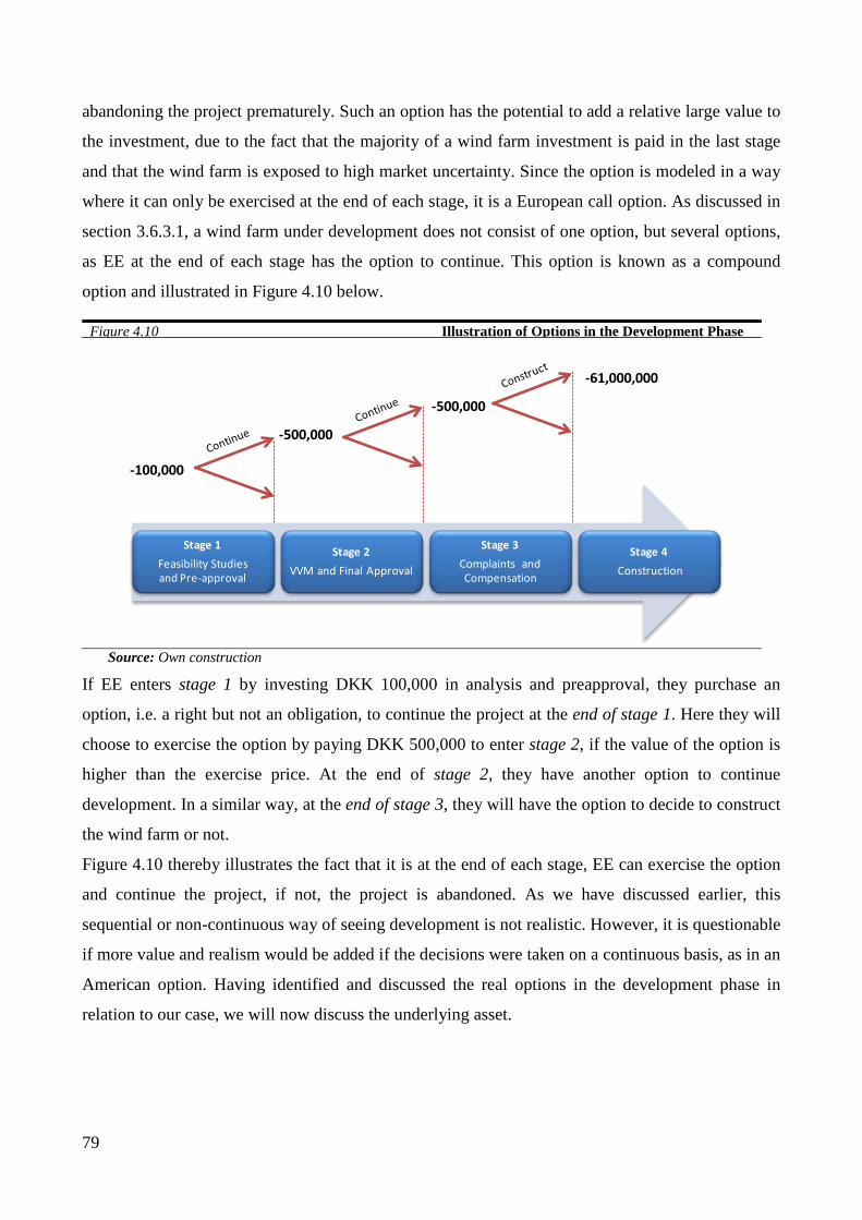
79

abandoning the project prematurely. Such an option has the potential to add a relative large value to

the investment, due to the fact that the majority of a wind farm investment is paid in the last stage

and that the wind farm is exposed to high market uncertainty. Since the option is modeled in a way

where it can only be exercised at the end of each stage, it is a European call option. As discussed in

section 3.6.3.1, a wind farm under development does not consist of one option, but several options,

as EE at the end of each stage has the option to continue. This option is known as a compound

option and illustrated in Figure 4.10 below.

Figure 4.10 Illustration of Options in the Development Phase


If EE enters stage 1 by investing DKK 100,000 in analysis and preapproval, they purchase an

option, i.e. a right but not an obligation, to continue the project at the end of stage 1. Here they will

choose to exercise the option by paying DKK 500,000 to enter stage 2, if the value of the option is

higher than the exercise price. At the end of stage 2, they have another option to continue

development. In a similar way, at the end of stage 3, they will have the option to decide to construct

the wind farm or not.

Figure 4.10 thereby illustrates the fact that it is at the end of each stage, EE can exercise the option

and continue the project, if not, the project is abandoned. As we have discussed earlier, this

sequential or non-continuous way of seeing development is not realistic. However, it is questionable

if more value and realism would be added if the decisions were taken on a continuous basis, as in an

American option. Having identified and discussed the real options in the development phase in

relation to our case, we will now discuss the underlying asset.




Stage 4Construction

-100,000

-500,000

-500,000

-61,000,000

80

4.4.4. Step 2: The Underlying Asset As discussed in chapter 3, it is possible to use the PV of the project as the underlying asset of the

real option. This means that the value of the underlying asset is the value of the operational phase

using the standard DCF model, discounted back to primo year 2010, shown in Formula 4.5 below.

This PV does not include the development and construction costs, as these are accounted for

separately in the binomial tree.

Formula 4.5 Present Value of Underlying Asset

𝐏𝐕𝟐𝟎𝟏𝟎 =∑𝐃𝐂𝐅𝐎𝐏(𝟏 + 𝐫𝐄)𝐧

𝐃𝐊𝐊 𝟓𝟕,𝟖𝟐𝟕,𝟐𝟓𝟏 =𝐃𝐊𝐊 𝟕𝟎,𝟒𝟕𝟗,𝟗𝟗𝟔

(𝟏 + 𝟎.𝟎𝟔𝟖𝟐)𝟑

𝑷𝑽𝟐𝟎𝟏𝟎: Present value 2010 = DKK 57,827,251

𝑭𝑪𝑭𝑶𝑷: DCF value of operational phase = DKK 70,479,996

𝒏: Periods = 3

𝒓𝑬: Cost of equity= 6.82%


4.4.5. Step 3: Uncertainty Estimation The market uncertainty is represented by the volatility of the underlying asset. Estimating this is the

most critical step in a ROV, since it is a main value driver and a parameter which clearly

distinguishes ROV from DCF based valuation models. At the same time, the challenge of

estimating the volatility is one of the main reasons that practitioners are reluctant to adapt ROV

models (Shockley 2007: 302). Therefore, in the following analysis, we make an effort to estimate

the volatility. This is done both to obtain a valid result and to oblige the worries of practitioners.

The analysis will start with some general considerations on volatility estimation, followed by a

discussion of the stochastic process and models available for volatility estimations. Based on this

we will estimate the volatility and discuss the estimate by comparison to several volatility peers.

4.4.5.1. Considerations on Volatility Estimation of a Wind Farm under Development

As discussed in chapter 3, the volatility can be estimated using either internal or external methods.

In the case of investments in natural resource projects, we recommended to use the external

approach, where the volatility is estimated from the commodity related to the investment. As wind

parks in Denmark are compensated with the market price of electricity plus a fixed subsidy, the

value of a wind park is highly correlated with the electricity price. We have therefore chosen the

price volatility of electricity as the twin-security for our volatility estimation. With regard to

practical implementation, this approach has the advantage of suggesting a volatility estimate which

is publicly available.

81

But due to the complex nature of electricity, the volatility of the electricity price is difficult to

estimate compared to many other commodities. Several models have been developed to forecast and

describe this, such as Pilipovic’s two-factor model (2007: 158-162), as well as Lucia and Schwartz’

(2002: 17-23) one-factor and two-factor models. Common for these models are their awareness of

the difference in the stochastic movements of the short term and long term electricity price. These

models thereby address the importance of discussing the stochastic process of electricity prices.

4.4.5.2. The Behavior of Electricity Prices

As described in chapter 2, the nature of the spot price for electricity is very different from other

commodities or financial assets, primarily due to its non-storability, which implies highly volatile

short term prices. The transmission system operators and utilities have developed tools that can

estimate the supply and demand on a given day and time within reasonable precision. However,

small deviations from the predictions (due to the short term supply or demand shifts) continuously

affect the spot price, resulting in constant small

deviations around a long term mean value. Inspired by

Pilipovic, we call this mean value the long term

equilibrium price (2007: 23). Sometimes short term

incidences occur that affect either the present supply or

demand to such an extent that a large “spike” occurs.60

Common for these short term deviations are that they

only change the level temporary, where after the spot price reverts back towards the long term

equilibrium price level, as can be seen from the graph (Pilipovic 2007: 28 and 109). When

estimating the volatility, an awareness of these dynamics is necessary, as it can easily be

misestimated if an appropriate model is not used. Furthermore, it is important that the stochastic

movement of the underlying asset is consistent with the modeling of the binomial tree, as the model

could otherwise misestimate the value of the option.

4.4.5.2.1. Stochastic Processes and Electricity Prices

The standard binomial model assumes that the value of underlying asset follows a geometric

Brownian motion. This assumption has been challenged for commodity prices, and alternative

processes have been suggested. The two most common alternatives are mean-reverting and jump

diffusion processes. The prior modeled has been a popular competitor to the geometric Brownian

motion. The idea behind mean reversion is that prices are somewhat interrelated and in the long run

60 One example of a spike that happened in DK East Wednesday the 16th of December 2009, with a spot price from 16.00-18.00 above € 1400/MWh representing an increase compared to the previous day and time of more than 1300% (www.nordpool.dk).

Time

Price

Long Term Equilibrium

Short Term Deviations

Spike

82

will revert towards a long term equilibrium price. This process implies that price changes are no

longer completely independent, but instead revert towards a long term equilibrium price with a

certain speed known as the mean reversion rate (Blanco and Soronow 2001a: 68). While intuitively

clear, a problem for the modeling of the process is the proper estimation of the mean reversion

rate.61 The idea of mean reversion is often mentioned in relation to the behavior of commodity

prices, based on an idea of a long term price that reflects the cost of production and the level of

demand of the commodity. The model can be applied to ROV, as demonstrated by Hahn and Dyer

(2004), but it is a rarity and as such seems to need special justification (Lander and Pinches 1998:

550). The second alternative process is the jump diffusion process, which is able to capture large or

sudden changes in the project value. The drawback of the model is its need for quite complex

calculus, as well as the problems of meaningfully modeling the jumps (Blanco and Soronow 2001b:

86). Despite the initial appeal of these more advanced price processes it has been argued by several

academics that the long term electricity price, which is the relevant variable in our case, follows a

geometric Brownian motion. Several studies have been undertaken to determine the stochastic processes of electricity prices such

as Lucia and Schwartz’ (2002) study of Nord Pool electricity prices. This paper studies the regular

patterns in the behavior of electricity prices and what the implications of these are for electricity

derivatives pricing. Lucia and Schwartz do this by studying the variation in prices using different

one-factor and two-factor models. In the one-factor models, the prices follow a mean-reverting

stochastic process. In the two-factor models, the short term variations of the prices follow a mean

reverting process, but the equilibrium prices are modeled either as arithmetic or geometric

Brownian motions. Their results indicated that the two-factor models have a better fit to the data.

This argument can be expanded by the ones found in Schwartz and Smith (2000: 895) and Pilipovic

(2007: 109) who claim that for long term investments, the long term factors should be the decisive

one, thereby making the assumption that long term electricity prices follow a geometric Brownian

motion valid. A similar argument is made in Pindyck (2000: 26), who claims that the geometric

Brownian motion can be used when modeling the long term behavior of commodity prices. In the

case of ROVs of renewable energy projects, Bøckman et al. (2007: 257) and Fleten et al. (2007:

805) also choose to model long term electricity prices as a geometric Brownian motions.

61 This can be further complicated by discussion such as whether or not mean reversion is constant or should change through time (Blanco and Soronow 2001a: 69).

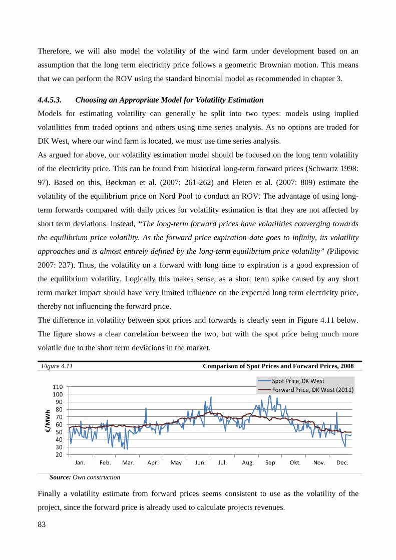
83

Therefore, we will also model the volatility of the wind farm under development based on an

assumption that the long term electricity price follows a geometric Brownian motion. This means

that we can perform the ROV using the standard binomial model as recommended in chapter 3.

4.4.5.3. Choosing an Appropriate Model for Volatility Estimation

Models for estimating volatility can generally be split into two types: models using implied

volatilities from traded options and others using time series analysis. As no options are traded for

DK West, where our wind farm is located, we must use time series analysis.

As argued for above, our volatility estimation model should be focused on the long term volatility

of the electricity price. This can be found from historical long-term forward prices (Schwartz 1998:

97). Based on this, Bøckman et al. (2007: 261-262) and Fleten et al. (2007: 809) estimate the

volatility of the equilibrium price on Nord Pool to conduct an ROV. The advantage of using long-

term forwards compared with daily prices for volatility estimation is that they are not affected by

short term deviations. Instead, “The long-term forward prices have volatilities converging towards

the equilibrium price volatility. As the forward price expiration date goes to infinity, its volatility

approaches and is almost entirely defined by the long-term equilibrium price volatility” (Pilipovic

2007: 237). Thus, the volatility on a forward with long time to expiration is a good expression of

the equilibrium volatility. Logically this makes sense, as a short term spike caused by any short

term market impact should have very limited influence on the expected long term electricity price,

thereby not influencing the forward price.

The difference in volatility between spot prices and forwards is clearly seen in Figure 4.11 below.

The figure shows a clear correlation between the two, but with the spot price being much more

volatile due to the short term deviations in the market.

Figure 4.11 Comparison of Spot Prices and Forward Prices, 2008


Finally a volatility estimate from forward prices seems consistent to use as the volatility of the

project, since the forward price is already used to calculate projects revenues.

Jan.

2030405060708090

100110

€/M

Wh

Spot Price, DK WestForward Price, DK West (2011)

Jan. Feb. Mar. Apr. May Jun. Jul. Aug. Sep. Okt. Nov. Dec.

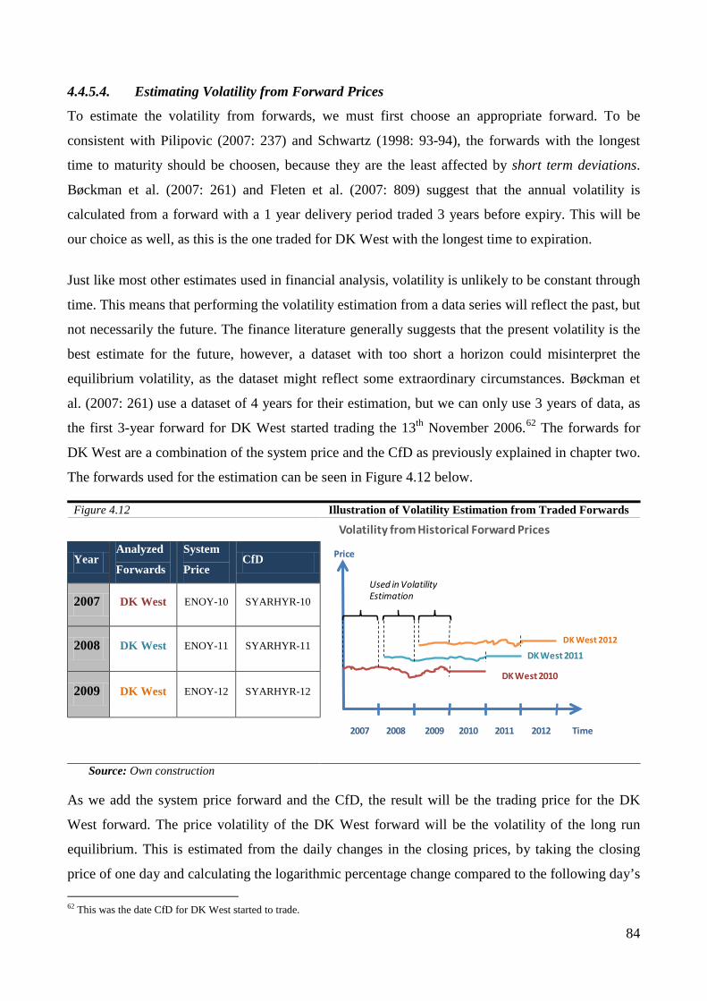
84

4.4.5.4. Estimating Volatility from Forward Prices

To estimate the volatility from forwards, we must first choose an appropriate forward. To be

consistent with Pilipovic (2007: 237) and Schwartz (1998: 93-94), the forwards with the longest

time to maturity should be choosen, because they are the least affected by short term deviations.

Bøckman et al. (2007: 261) and Fleten et al. (2007: 809) suggest that the annual volatility is

calculated from a forward with a 1 year delivery period traded 3 years before expiry. This will be

our choice as well, as this is the one traded for DK West with the longest time to expiration.

Just like most other estimates used in financial analysis, volatility is unlikely to be constant through

time. This means that performing the volatility estimation from a data series will reflect the past, but

not necessarily the future. The finance literature generally suggests that the present volatility is the

best estimate for the future, however, a dataset with too short a horizon could misinterpret the

equilibrium volatility, as the dataset might reflect some extraordinary circumstances. Bøckman et

al. (2007: 261) use a dataset of 4 years for their estimation, but we can only use 3 years of data, as

the first 3-year forward for DK West started trading the 13th November 2006.62 The forwards for

DK West are a combination of the system price and the CfD as previously explained in chapter two.

The forwards used for the estimation can be seen in Figure 4.12 below.

Figure 4.12 Illustration of Volatility Estimation from Traded Forwards

Year Analyzed

Forwards

System

Price CfD

2007 DK West ENOY-10 SYARHYR-10




As we add the system price forward and the CfD, the result will be the trading price for the DK

West forward. The price volatility of the DK West forward will be the volatility of the long run

equilibrium. This is estimated from the daily changes in the closing prices, by taking the closing

price of one day and calculating the logarithmic percentage change compared to the following day’s 62 This was the date CfD for DK West started to trade.

2007 2008 2009 2010 2011 2012 Time

Volatility from Historical Forward Prices

DK West 2011

DK West 2010

DK West 2012

Used in VolatilityEstimation

Price

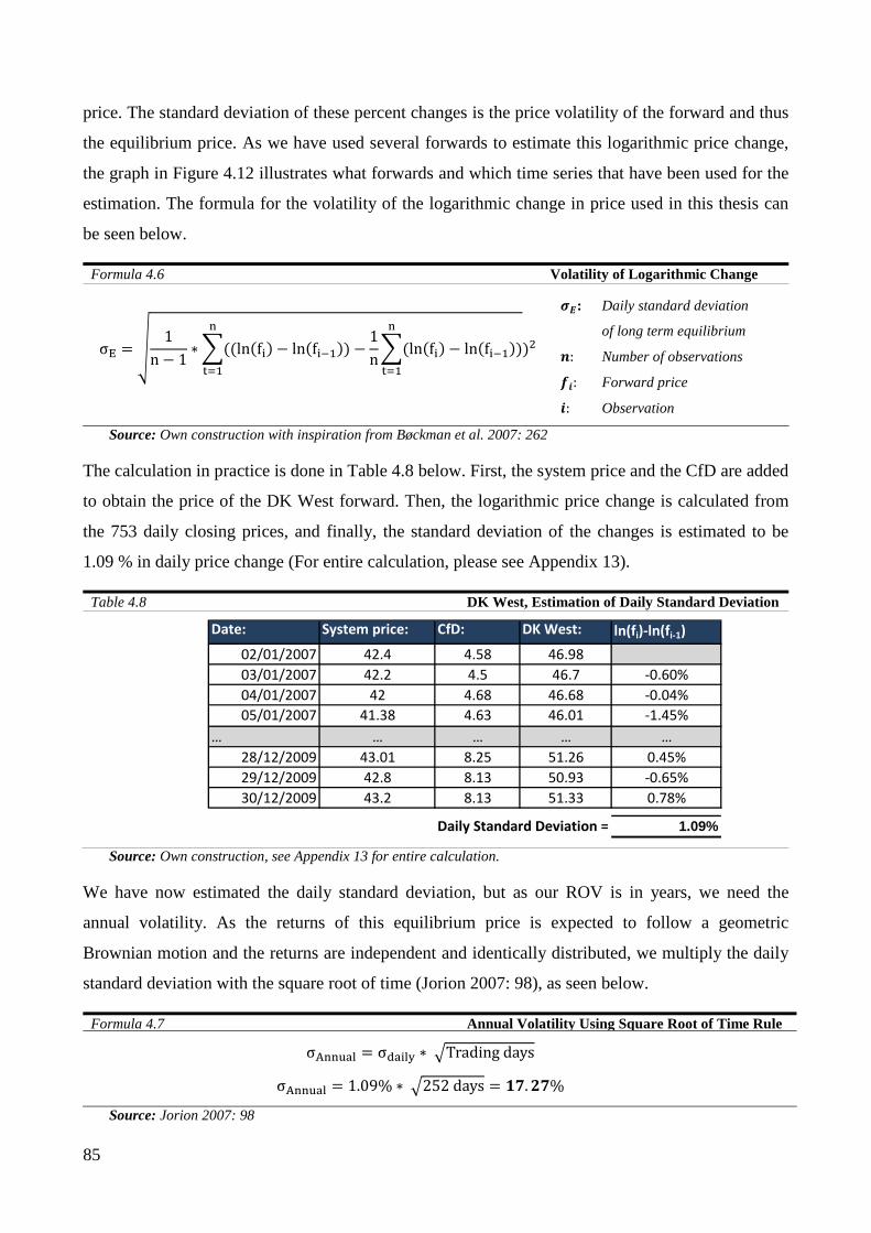
85

price. The standard deviation of these percent changes is the price volatility of the forward and thus

the equilibrium price. As we have used several forwards to estimate this logarithmic price change,

the graph in Figure 4.12 illustrates what forwards and which time series that have been used for the

estimation. The formula for the volatility of the logarithmic change in price used in this thesis can

be seen below.

Formula 4.6 Volatility of Logarithmic Change

σE = �1

n − 1∗�((ln(fi)− ln(fi−1))

n

t=1

−1n�(ln(fi)− ln(fi−1))n

t=1

)2

𝝈𝑬: Daily standard deviation

of long term equilibrium

𝒏: Number of observations

𝒇𝒊: Forward price

𝒊: Observation

Source: Own construction with inspiration from Bøckman et al. 2007: 262

The calculation in practice is done in Table 4.8 below. First, the system price and the CfD are added

to obtain the price of the DK West forward. Then, the logarithmic price change is calculated from

the 753 daily closing prices, and finally, the standard deviation of the changes is estimated to be

1.09 % in daily price change (For entire calculation, please see Appendix 13).

Table 4.8 DK West, Estimation of Daily Standard Deviation

Source: Own construction, see Appendix 13 for entire calculation.

We have now estimated the daily standard deviation, but as our ROV is in years, we need the

annual volatility. As the returns of this equilibrium price is expected to follow a geometric

Brownian motion and the returns are independent and identically distributed, we multiply the daily

standard deviation with the square root of time (Jorion 2007: 98), as seen below.

Formula 4.7 Annual Volatility Using Square Root of Time Rule

σAnnual = σdaily ∗ �Trading days

σAnnual = 1.09% ∗ �252 days = 𝟏𝟕.𝟐𝟕%

Source: Jorion 2007: 98

Date: System price: CfD: DK West: ln(fi)-ln(fi-1)02/01/2007 42.4 4.58 46.9803/01/2007 42.2 4.5 46.7 -0.60%04/01/2007 42 4.68 46.68 -0.04%05/01/2007 41.38 4.63 46.01 -1.45%

… … … … …28/12/2009 43.01 8.25 51.26 0.45%29/12/2009 42.8 8.13 50.93 -0.65%30/12/2009 43.2 8.13 51.33 0.78%

1.09%Daily Standard Deviation =

86

Since the volatility estimate is a fundamental value driver of an option, we will now assess this

estimate in comparison to other relevant volatilities estimates.

4.4.5.5. Comparison of Volatility Estimate

Based on the volatility of forward prices, the annual electricity price volatility is calculated to be

17.27% from 2007-2009. As a way to test the reason and validity of this estimate, we have chosen

to calculate several volatility comparisons, which are shown in Table 4.9 below.

It is possible that specific events in DK West during 2007-2009 have influenced the historical data

set significantly, therefore we perform a validation of the dataset by comparing it to the historical

volatility from forwards calculated on the Nord Pool system price and the German Phelix price.63

As explained in chapter two, DK West is a “buffer” market between the Nordic and the German

electricity market, hence our expectation is that the volatility is in-between the two estimates.

Table 4.9 Forward Volatility Peers

Market Validate: Method Vol. Deviation from

Estimate: Expected:

Forward

Price

DK

West

Logarithmic change on annual

forwards (2007-2009) 17.27 % - -

Peer 1 Nordic Dataset Forward volatility, System Price 21.41 % + 4.14 PP Higher

Peer 2 German Dataset Forward volatility, Phelix Price 15.97 % - 1.30 PP Lower

Source: Own construction (See Data CD for calculations).

As can be seen from the table above, the volatility of the Nordic market is 4.14 percentage points

(PP) above the DK West estimate and the German market is 1.30 PP below. The higher Nordic

volatility is a consequence of the instability of the supply of cheap energy in the Nordic countries,

depending in particular on the amount of hydropower generated in Swedish and Norwegian rivers

causing a more volatile price, when compared to the more stable and easier controllable German

thermal energy sources (IBT Wind 2006: 9). Based on the above figures, the volatility estimate of

17.27% for DK West seems plausible, which indicates that our dataset has not been disturbed by

any large events within the sample period, compared to these peers.

To test the methodology of estimating volatility, we will use implied volatilities from traded

options. As no option is traded for DK West, it is not possible to estimate it for this market.

63 Phelix is an abbreviation for Physical Electricity Index. This is an equilibrium price of electricity between Germany and Austria. The derivatives are traded on the German power exchange EEX. The Phelix price is chosen as there are no options traded only for the German market.

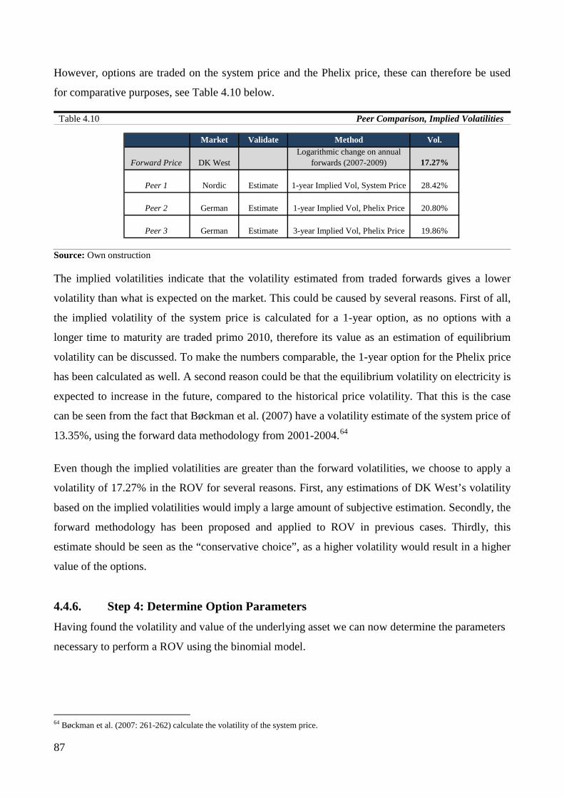
87

However, options are traded on the system price and the Phelix price, these can therefore be used

for comparative purposes, see Table 4.10 below.

Table 4.10 Peer Comparison, Implied Volatilities

Source: Own onstruction

The implied volatilities indicate that the volatility estimated from traded forwards gives a lower

volatility than what is expected on the market. This could be caused by several reasons. First of all,

the implied volatility of the system price is calculated for a 1-year option, as no options with a

longer time to maturity are traded primo 2010, therefore its value as an estimation of equilibrium

volatility can be discussed. To make the numbers comparable, the 1-year option for the Phelix price

has been calculated as well. A second reason could be that the equilibrium volatility on electricity is

expected to increase in the future, compared to the historical price volatility. That this is the case

can be seen from the fact that Bøckman et al. (2007) have a volatility estimate of the system price of

13.35%, using the forward data methodology from 2001-2004.64

Even though the implied volatilities are greater than the forward volatilities, we choose to apply a

volatility of 17.27% in the ROV for several reasons. First, any estimations of DK West’s volatility

based on the implied volatilities would imply a large amount of subjective estimation. Secondly, the

forward methodology has been proposed and applied to ROV in previous cases. Thirdly, this

estimate should be seen as the “conservative choice”, as a higher volatility would result in a higher

value of the options.

4.4.6. Step 4: Determine Option Parameters Having found the volatility and value of the underlying asset we can now determine the parameters

necessary to perform a ROV using the binomial model.

64 Bøckman et al. (2007: 261-262) calculate the volatility of the system price.

Market Validate Method Vol.

Forward Price DK WestLogarithmic change on annual

forwards (2007-2009) 17.27%

Peer 1 Nordic Estimate 1-year Implied Vol, System Price 28.42%

Peer 2 German Estimate 1-year Implied Vol, Phelix Price 20.80%

Peer 3 German Estimate 3-year Implied Vol, Phelix Price 19.86%

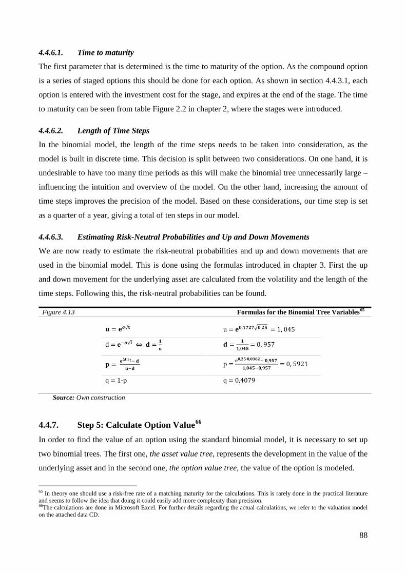
88

4.4.6.1. Time to maturity

The first parameter that is determined is the time to maturity of the option. As the compound option

is a series of staged options this should be done for each option. As shown in section 4.4.3.1, each

option is entered with the investment cost for the stage, and expires at the end of the stage. The time

to maturity can be seen from table Figure 2.2 in chapter 2, where the stages were introduced.

4.4.6.2. Length of Time Steps

In the binomial model, the length of the time steps needs to be taken into consideration, as the

model is built in discrete time. This decision is split between two considerations. On one hand, it is

undesirable to have too many time periods as this will make the binomial tree unnecessarily large –

influencing the intuition and overview of the model. On the other hand, increasing the amount of

time steps improves the precision of the model. Based on these considerations, our time step is set

as a quarter of a year, giving a total of ten steps in our model.

4.4.6.3. Estimating Risk-Neutral Probabilities and Up and Down Movements

We are now ready to estimate the risk-neutral probabilities and up and down movements that are

used in the binomial model. This is done using the formulas introduced in chapter 3. First the up

and down movement for the underlying asset are calculated from the volatility and the length of the

time steps. Following this, the risk-neutral probabilities can be found.

Figure 4.13 Formulas for the Binomial Tree Variables65

𝐮 = 𝐞𝛔√𝐭 u = 𝐞𝟎,𝟏𝟕𝟐𝟕�𝟎,𝟐𝟓 = 1, 045

d = 𝐞−𝛔√𝐭 ⇔ 𝐝 = 𝟏𝐮 𝐝 = 𝟏

𝟏,𝟎𝟒𝟓 = 0, 957

𝐩 = 𝐞∆𝐭∙𝐫𝐟− 𝐝 𝐮−𝐝

p = 𝐞𝟎,𝟐𝟓∙𝟎,𝟎𝟑𝟔𝟐− 𝟎,𝟗𝟓𝟕 𝟏,𝟎𝟒𝟓−𝟎,𝟗𝟓𝟕

= 0, 5921

q = 1-p q = 0,4079


4.4.7. Step 5: Calculate Option Value66 In order to find the value of an option using the standard binomial model, it is necessary to set up

two binomial trees. The first one, the asset value tree, represents the development in the value of the

underlying asset and in the second one, the option value tree, the value of the option is modeled.

65 In theory one should use a risk-free rate of a matching maturity for the calculations. This is rarely done in the practical literature and seems to follow the idea that doing it could easily add more complexity than precision. 66The calculations are done in Microsoft Excel. For further details regarding the actual calculations, we refer to the valuation model on the attached data CD.

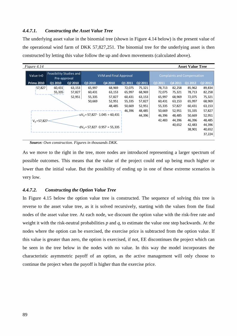
89

4.4.7.1. Constructing the Asset Value Tree

The underlying asset value in the binomial tree (shown in Figure 4.14 below) is the present value of

the operational wind farm of DKK 57,827,251. The binomial tree for the underlying asset is then

constructed by letting this value follow the up and down movements (calculated above).

Figure 4.14 Asset Value Tree

Source: Own construction. Figures in thousands DKK.

As we move to the right in the tree, more nodes are introduced representing a larger spectrum of

possible outcomes. This means that the value of the project could end up being much higher or

lower than the initial value. But the possibility of ending up in one of these extreme scenarios is

very low.

4.4.7.2. Constructing the Option Value Tree

In Figure 4.15 below the option value tree is constructed. The sequence of solving this tree is

reverse to the asset value tree, as it is solved recursively, starting with the values from the final

nodes of the asset value tree. At each node, we discount the option value with the risk-free rate and

weight it with the risk-neutral probabilities p and q, to estimate the value one step backwards. At the

nodes where the option can be exercised, the exercise price is subtracted from the option value. If

this value is greater than zero, the option is exercised, if not, EE discontinues the project which can

be seen in the tree below in the nodes with no value. In this way the model incorporates the

characteristic asymmetric payoff of an option, as the active management will only choose to

continue the project when the payoff is higher than the exercise price.

Primo 2010 Q1 2010 Q2 2010 Q3 2010 Q4 2010 Q1 2011 Q2 2011 Q3 2011 Q4 2011 Q1 2012 Q2 201257,827 60,431 63,153 65,997 68,969 72,075 75,321 78,713 82,258 85,962 89,834

55,335 57,827 60,431 63,153 65,997 68,969 72,075 75,321 78,713 82,258 52,951 55,335 57,827 60,431 63,153 65,997 68,969 72,075 75,321

50,669 52,951 55,335 57,827 60,431 63,153 65,997 68,969 48,485 50,669 52,951 55,335 57,827 60,431 63,153

46,396 48,485 50,669 52,951 55,335 57,827 44,396 46,396 48,485 50,669 52,951

42,483 44,396 46,396 48,485 40,652 42,483 44,396

38,901 40,652 37,224

Feasibility Studies and Pre-approval

Value t=0 VVM and Final Approval Complaints and Compensation

V0 =57,827

uV0 = 57,827 . 1.045 = 60,431

dV0 = 57,827 . 0.957 = 55,335

90

Figure 4.15 Option Value Tree

Source: Own construction, Figures in thousands DKK.

The real options value of the wind farm under development (only including the market uncertainty)

can be seen in the far left node in the tree, and is equal to DKK 3,324,569.67 However, be aware

that this is a hypothetical value, since the probability of failure has not been included.

4.4.8. Step 6: Sensitivity Analysis The final step in the six step model is to conduct a sensitivity analysis on the main value driver of

the ROV, which is the volatility estimate of the underlying asset, as shown in Figure 4.16 below.

Figure 4.16 Sensitivity Analysis of Volatility Estimate


As can be seen above, the real option value is highly sensitive to the volatility. A 10% increase of

the estimate (equal to a nominal change in volatility of approximately 2 PP) causes a 9.7% increase

in real option value. This makes sense, as a higher volatility increases the possibility of ending up

with a very valuable wind farm, whereas the loss can never be greater than the option value.

67 The real options valuation results in a net present value due to discounting of cash flows and costs being subtracted. The term NPV has not been used in regard to real option valuations to avoid confusion with DCF based models.

Primo 2010 Q1 2010 Q2 2010 Q3 2010 Q4 2010 Q1 2011 Q2 2011 Q3 2011 Q4 2011 Q1 2012 Q2 20123,325 4,703 6,279 8,669 10,858 13,313 15,990 19,347 22,352 25,512 28,834

1,645 2,520 4,186 5,684 7,536 9,723 12,709 15,415 18,263 21,258 412 1,394 2,104 3,121 4,528 6,840 9,063 11,625 14,321

232 395 674 1,148 2,509 3,765 5,547 7,969 - - - 435 741 1,263 2,153

- - - - - - - - - - -

- - - - - - -

- - -

EX 100 500 500 61,000

Value t=0 Feasibility Studies and Pre-approval

VVM and Final Approval Complaints and Compensation

89,834-61,000 = 28,834

(0.5921*15,990+0.4079*9,723)/1.0091 = 13,313

MAX[((0.5921*8,669+4,186*0.4079)/1.0091-500);0] = 6,279

-20% -10% 17.62% +10% +20%Volatility 14.10% 15.86% 17.62% 19.38% 21.14%ROV kr 2,667,486 kr 2,998,610 kr 3,324,569 kr 3,646,250 kr 3,964,440Relative Change -19.8% -9.8% - 9.7% 19.2%

Volatility

91

4.5 Quadranomial Real Options Valuation In the following section the value of the wind farm is found including both events and market

uncertainty, by use of the quadranomial approach. The quadranomial approach is an extension to

the binomial approach, and requires relatively little effort once the binomial option parameters

have been estimated.

4.5.1. Introduction We have now calculated the value of a wind farm under development, including events in the

ENPV model and market uncertainty in the binomial ROV. Both of the two models provide

misguiding results, as it is more realistic to include both events and market uncertainty to value the

wind farm under development.

What should be clear from the two previous valuations is the distinct nature of market uncertainty

and events. Where market uncertainty is modeled as a continuous process, as it is resolved

continuously over time, the events are model on a non-continuous basis. The difference between the

two is demonstrated in Figure 4.17 below, where the market uncertainty develops smoothly through

time, whereas the outcome of the event is resolved when the information becomes available.

Figure 4.17 Resolution of Uncertainty and Events over Time


Furthermore the figure shows how market uncertainty increases over time, whereas the uncertainty

with regard to the events is resolved over time as the wind farm is either approved or denied. The

distinct character of the market uncertainty and events is the reason that they have been treated

separately until this point in the valuation. As mentioned in chapter 3, instead of combining the two

into a single measure, we continue to keep them separated in our ROV – in line with Copeland and

Time

Uncertainty

Event

Market Uncertainty

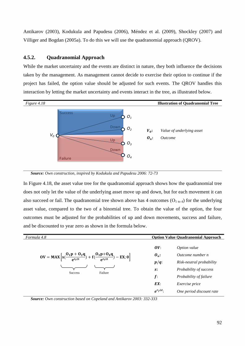
92

Antikarov (2003), Kodukula and Papudesu (2006), Méndez et al. (2009), Shockley (2007) and

Villiger and Bogdan (2005a). To do this we will use the quadranomial approach (QROV).

4.5.2. Quadranomial Approach While the market uncertainty and the events are distinct in nature, they both influence the decisions

taken by the management. As management cannot decide to exercise their option to continue if the

project has failed, the option value should be adjusted for such events. The QROV handles this

interaction by letting the market uncertainty and events interact in the tree, as illustrated below.

Figure 4.18 Illustration of Quadranomial Tree

𝑽𝟎: Value of underlying asset

𝑶𝒏: Outcome

Source: Own construction, inspired by Kodukula and Papudesu 2006: 72-73

In Figure 4.18, the asset value tree for the quadranomial approach shows how the quadranomial tree

does not only let the value of the underlying asset move up and down, but for each movement it can

also succeed or fail. The quadranomial tree shown above has 4 outcomes (O1 to 4) for the underlying

asset value, compared to the two of a binomial tree. To obtain the value of the option, the four

outcomes must be adjusted for the probabilities of up and down movements, success and failure,

and be discounted to year zero as shown in the formula below.

Formula 4.8 Option Value Quadranomial Approach

𝐎𝐕 = 𝐌𝐀𝐗 �𝐬(𝐎𝟏𝐩 + 𝐎𝟐𝐪

𝐞𝐫𝐟∆𝐭) + 𝐟(

𝐎𝟑𝐩+𝐎𝟒𝐪𝐞𝐫𝐟∆𝐭

) − 𝐄𝐗;𝟎�

Success Failure

𝑶𝑽: Option value

𝑶𝒏: Outcome number n

𝒑/𝒒: Risk-neutral probability

𝒔: Probability of success

𝒇: Probability of failure

𝑬𝑿: Exercise price

𝒆𝒓𝒇∆𝒕: One period discount rate

Source: Own construction based on Copeland and Antikarov 2003: 332-333

V0

O1Success

Failure

Up

Down

Up

Down

O2

O3

O4

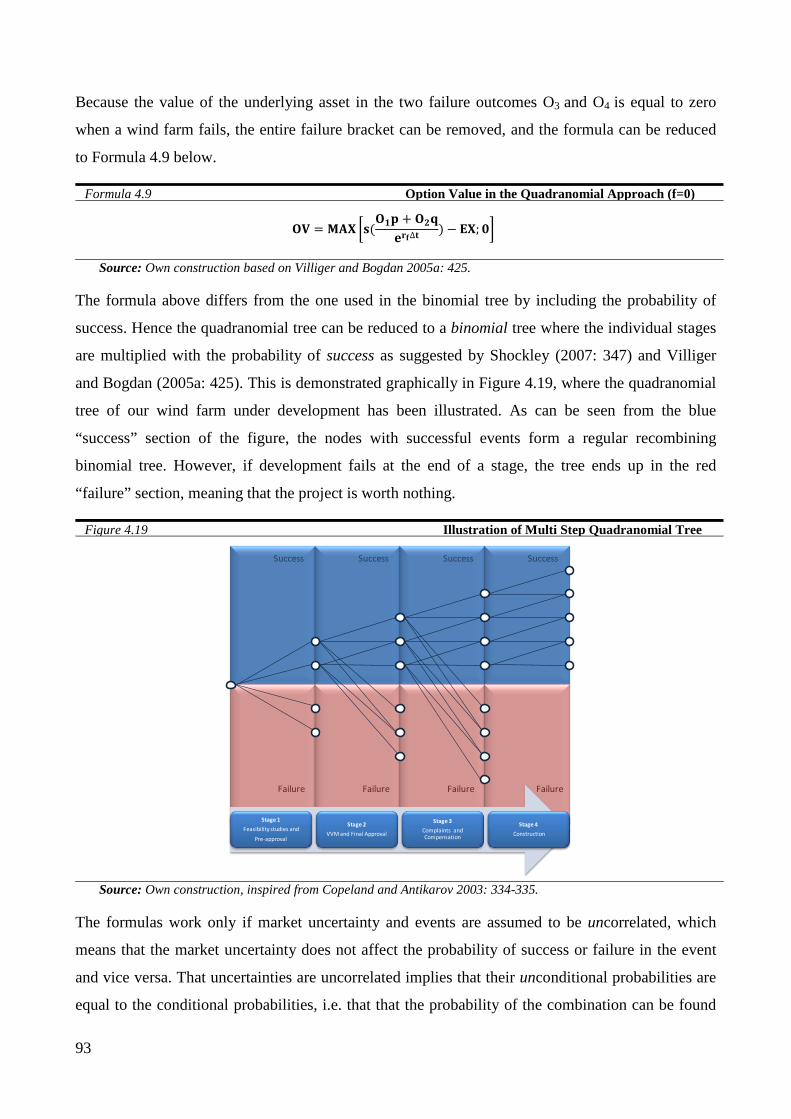
93

Because the value of the underlying asset in the two failure outcomes O3 and O4 is equal to zero

when a wind farm fails, the entire failure bracket can be removed, and the formula can be reduced

to Formula 4.9 below.

Formula 4.9 Option Value in the Quadranomial Approach (f=0)

𝐎𝐕 = 𝐌𝐀𝐗 �𝐬(𝐎𝟏𝐩 + 𝐎𝟐𝐪

𝐞𝐫𝐟∆𝐭) − 𝐄𝐗;𝟎�

Source: Own construction based on Villiger and Bogdan 2005a: 425.

The formula above differs from the one used in the binomial tree by including the probability of

success. Hence the quadranomial tree can be reduced to a binomial tree where the individual stages

are multiplied with the probability of success as suggested by Shockley (2007: 347) and Villiger

and Bogdan (2005a: 425). This is demonstrated graphically in Figure 4.19, where the quadranomial

tree of our wind farm under development has been illustrated. As can be seen from the blue

“success” section of the figure, the nodes with successful events form a regular recombining

binomial tree. However, if development fails at the end of a stage, the tree ends up in the red

“failure” section, meaning that the project is worth nothing.

Figure 4.19 Illustration of Multi Step Quadranomial Tree

Source: Own construction, inspired from Copeland and Antikarov 2003: 334-335.

The formulas work only if market uncertainty and events are assumed to be uncorrelated, which

means that the market uncertainty does not affect the probability of success or failure in the event

and vice versa. That uncertainties are uncorrelated implies that their unconditional probabilities are

equal to the conditional probabilities, i.e. that that the probability of the combination can be found

Stage 1 Analysis and Preapproval



Stage 4Construction

Success Success Success Success

Failure Failure Failure Failure

Stage 1 Feasibility studies and

Pre-approval



Stage 4Construction

94

by multiplying them with each other (Copeland and Antikarov 2003: 283).68 That market

uncertainty and events are uncorrelated means that an increase in value should not increase the

possibility that the municipality approves the wind farm.

4.5.3. Calculation of Option Value With the QROV explained, we are now ready to model the value of the wind farm under

development including both market uncertainty and events. This approach, just like the regular

binomial tree, requires the construction of an underlying asset value tree and an option value tree.

But to implement the model, we will need to modify our earlier presented six step model, as seen in

Figure 4.20.

Figure 4.20 Modified Six Step Model for QROV


As shown with red above, we need to modify step 3 to include the events and probabilities

estimations. Furthermore, step 5 now includes the construction of a quadranomial option value tree.

The rest of the stages all remain the same.

As we have already estimated the events and probabilities, we will now turn to the construction of

the quadranomial option value tree.

The quadranomial option value tree is constructed from the asset value tree (in section 4.4.7.1), as

this has not changed. The tree is solved recursively, just like the binomial option value tree in

Figure 4.15. The major difference is that the events are included.

The logic behind the tree is as follows. EE enters stage 1 by purchasing an option primo 2010 for

DKK 100,000. Ultimo Q2 2010 the pre-municipality approval will be given with a 50% chance,

which means that this is the probability for EE to pass the stage. In the meantime, the market can

either have moved up or down. If the value of the option (given the market condition) is worth more

than the exercise price to enter stage 2, which is 500,000, then EE will exercise the option (invest 68 Copeland and Antikarov 2003: 279-86 also discuss a quadranomial approach with two correlated uncertainties and one with two uncorrelated uncertainties following a geometric Brownian motion.




uncertaintyIdentify events and

determine probabilities

Step 1Framing ROV

Justify ROV




phase

Step 6Sensitivity Analysis


Discuss results


Value


Build quadranomial option value tree



Determine Op Parameters

Step 4

Time to maturity

Length of time steps

Risk neutral prob.

Determine Option Parameters

95

DKK 500,000) and move on to the next stage. From the option value tree in Figure 4.21 below, it is

shown that in the end of stage 1, two out of the three nodes have a positive option value after

subtracting the exercise price to enter stage 2, and development is therefore continued, whereas the

last node is zero and development is therefore discontinued.

Figure 4.21 Option Value Tree


The value of a wind farm under development using QROV is DKK 431,289, which is

approximately DKK 500,000 more than the value found using the ENPV previously. This clearly

shows that a significant value can be added by perceiving a wind farm as a real option and this

difference can be perceived as the value of decision making. In our particular case the difference

between the results leads to two different strategies. Where the ENPV suggests not to invest – the

ROV suggests to invest. The increase in value demonstrates that it makes sense to think of wind

farms under development as real options to conduct a proper valuation.

4.5.4. Sensitivity Analysis In the above valuation, we combined the events and the market uncertainty in the development

phase. We will now conduct a sensitivity analysis of how the events and market uncertainty

influence the value of the result of the QROV approach, as shown in Figure 4.22 below.

Primo 2010 Q1 2010 Q2 2010 Q3 2010 Q4 2010 Q1 2011 Q2 2011 Q3 2011 Q4 2011 Q1 2012 Q2 2012431 770 1,082 3,419 4,294 5,276 6,346 15,478 17,882 20,410 23,067

196 334 1,629 2,224 2,965 3,839 10,167 12,332 14,610 17,006 - 527 801 1,199 1,761 5,472 7,251 9,300 11,457

83 141 240 409 2,007 3,012 4,437 6,375 - - - 348 593 1,011 1,722

- - - - - - - - - - -

- - - - - - -

- - -

Prob. 100% 100% 50% 100% 100% 100% 50% 100% 100% 100% 80%EX 100 500 500 61,000



MAX[((0.5921*3,419+1,629*0.4079)/1.0091-500);0]*0.5 = 1,082

96

Figure 4.22 Sensitivity Analysis QROV


From the sensitivity analysis we can see that the changes in the probabilities have a large impact on

the value. The volatility is also a very important value driver, and can potentially change the value

significantly. Thus both market uncertainty and events should be included in a valuation, in order to

obtain a superior valuation.

4.6 Recapitulation In this chapter, we have valued the wind farm under development using the models discussed in

chapter 3. Initially, we found the value of the operational wind phase using a four step model, as it

is necessary for finding the value of the wind farm under development. In the valuation of the

operational phase, it became clear that despite the standard DCF model being viewed as a simple

and intuitive framework for financial valuations, the actual calculation of the variables in the model,

such as the cost of equity, is no easy task. Based on the value of the operational phase, we

calculated the value of a wind farm under development, taking into account the failure events

during the development phase in the ENPV model. ENPV was preferred over DTA due to DTA’s

problems of a changing discount rate. The ENPV gave a negative NPV, implying that the

investment in the development of wind farm should not be undertaken. The result did, however, not

take into account that EE can decide on whether or not they want to continue at the end of each

stage.

To address the lacking ability to handle the decisions in ENPV, we introduced ROV. The ROV was

performed using the six step model. First this six step model was introduced with a regular binomial

-20% -10% 50.00% +10% +20%Probability Stage 1 40% 45% 50% 55% 60%QROV kr 325,032 kr 378,161 kr 431,289 kr 484,418 kr 537,547Relative Change -25% -12% - 12% 25%

-20% -10% 50.00% +10% +20%Probability Stage 2 40.00% 45.00% 50.00% 55.00% 60.00%QROV kr 284,096 kr 357,693 kr 431,289 kr 504,886 kr 578,482Relative Change -34.1% -17.1% - 17.1% 34.1%

-20% -10% 80.00% +10% +20%Probability Stage 3 64.00% 72.00% 80.00% 88.00% 96.00%QROV kr 266,741 kr 349,015 kr 431,289 kr 513,564 kr 595,838Relative Change -38.2% -19.1% - 19.1% 38.2%

-20% -10% 17.62% +10% +20%Volatility 14.10% 15.86% 17.62% 19.38% 21.14%QROV kr 303,471 kr 368,090 kr 431,289 kr 493,353 kr 554,507Relative Change -29.6% -14.7% - 14.4% 28.6%

Volatility




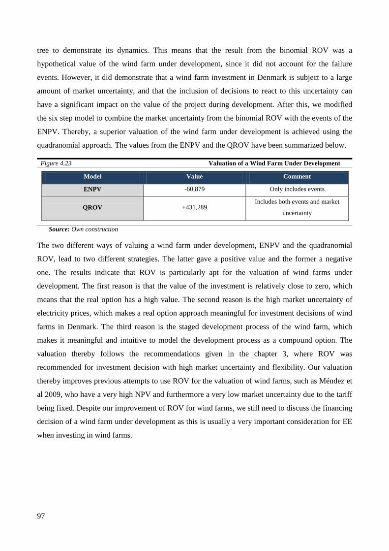
97

tree to demonstrate its dynamics. This means that the result from the binomial ROV was a

hypothetical value of the wind farm under development, since it did not account for the failure

events. However, it did demonstrate that a wind farm investment in Denmark is subject to a large

amount of market uncertainty, and that the inclusion of decisions to react to this uncertainty can

have a significant impact on the value of the project during development. After this, we modified

the six step model to combine the market uncertainty from the binomial ROV with the events of the

ENPV. Thereby, a superior valuation of the wind farm under development is achieved using the

quadranomial approach. The values from the ENPV and the QROV have been summarized below.

Figure 4.23 Valuation of a Wind Farm Under Development

Model Value Comment

ENPV -60,879 Only includes events

QROV +431,289 Includes both events and market

uncertainty


The two different ways of valuing a wind farm under development, ENPV and the quadranomial

ROV, lead to two different strategies. The latter gave a positive value and the former a negative

one. The results indicate that ROV is particularly apt for the valuation of wind farms under

development. The first reason is that the value of the investment is relatively close to zero, which

means that the real option has a high value. The second reason is the high market uncertainty of

electricity prices, which makes a real option approach meaningful for investment decisions of wind

farms in Denmark. The third reason is the staged development process of the wind farm, which

makes it meaningful and intuitive to model the development process as a compound option. The

valuation thereby follows the recommendations given in the chapter 3, where ROV was

recommended for investment decision with high market uncertainty and flexibility. Our valuation

thereby improves previous attempts to use ROV for the valuation of wind farms, such as Méndez et

al 2009, who have a very high NPV and furthermore a very low market uncertainty due to the tariff

being fixed. Despite our improvement of ROV for wind farms, we still need to discuss the financing

decision of a wind farm under development as this is usually a very important consideration for EE

when investing in wind farms.

98

5 Valuation Including the Financing Decision Until now, the large amount of debt which is typically used to finance wind farms has been ignored.

In the following chapter, we introduce the effect that debt has on the value of the project and

discuss how the models from the previous chapters can handle debt financing.

5.1 The Financing Decision is Important In chapter 2 we introduced project finance as European Energy’s typical way of raising debt for

their projects. Until now debt has been ignored, as we have performed all the previous calculations

assuming a pure equity financing of the project. This separation was done to focus on the

investment decision instead of the financing decision, as we discussed and applied the individual

valuation models.

5.1.1. European Energy’s Advantages from Using Project Finance Project financing is different from traditional corporate financing in several ways that influence the

value of the project. Project financing is defined as a project with non-recourse debt that is not

supported by the project’s sponsors, but only by the underlying cash flow of the project itself. In our

case, a small onshore wind farm in a developed country, there are two particularly notable features

of a project financing. The first is the high initial leverage ratios between 60 to 90% that are paid

down through the life of the project, resulting in large changes in the debt-equity ratio. The second

feature is that each wind farm is structured as a special purpose vehicle (SPV) making it possible to

let the project service the debt, instead of the company.

These two features of project finance create specific advantages for EE. The structuring as a SPV

makes it easier for the lenders to monitor the project, as they can focus primarily on the project risk

and do not have to monitor the sponsor as closely. In addition the set up ensures that high risk

projects do not “bankrupt” low risk projects and as such each project can be dealt with individually.

The structuring of the wind farm as a SPV is what makes a high leverage possible (Brealey et al.

1996: 34). The high leverage has two significant advantages for EE. The first advantage is the

interest tax shield (ITS) it generates from the high interest payments on the loan. The ITS is an

expression of the amount of the interest rate payments, which you can deduct from the income tax

of the project (Shah and Thakor 1987: 221). The second advantage is the possibility to build up a

larger asset base as more capital can be raised. The latter could alternatively be done by selling

equity, but this would mean that the control of the company would need to be shared with outsiders

99

(Chemmanur and John 1992: 402). There can also be disadvantages of project financing, if, for

example, a project has high bankruptcy costs, or from the preclusion of establishing an optimal

leverage for the entire company. However, these two disadvantages are irrelevant for wind farm

investments.

It is important to note that the project financing is not undertaken until the decision to construct the

wind farm has been taken. This means that it is only the operational phase that is debt financed. But

as the underlying asset of the wind farm under development is the operational wind farm, the value

of a project under development will change due to the debt. Therefore, we start by valuing the

impact of the financing decision in the operational phase, followed by its inclusion in the

development phase.

5.2 Models for Valuing Financial Side Effects The value of the project in the operational phase was previously calculated using the standard DCF

model. This model usually accounts for the value created by financing decisions by adjusting the

discount rate. This adjustment is not based on the difference in cost between debt and equity since,

as stated in Miller and Modigliani’s proposition II (1958: 268-272), the return that shareholders

demand increases with an increasing debt-equity ratio to reflect the greater risk that they are

exposed to.69 The reduction in the opportunity cost of capital due to debt financing is thus offset

causing a constant relationship. Instead the adjustment is based on the indirect side effects of the

financing decision, such as tax deductibility of interest payments, as acknowledged by Modigliani-

Miller. The standard way of recognizing this side effect is by the weighted average cost of capital

(WACC) seen in Formula 5.1 below.

Formula 5.1 Weighted Average Cost of Capital

𝐖𝐀𝐂𝐂 = 𝐫𝐃(𝟏 − 𝐓𝐜)𝐃𝐕

+ 𝐫𝐄𝐄𝐕

𝒓𝑫: Cost of debt

𝒓𝑬: Cost of equity

𝑻𝒄: Marginal corporate tax rate

𝑫: Debt to total capitalization ratio

𝑬: Equity to total capitalization ratio

𝑽: Value of company

Source: Brealey et al. 2006: 461.

As shown above, WACC lowers the costs of debt with the corporate tax rate thereby including the

ITS. This implies that WACC is reduced by increasing the leverage, which could lead to believe 69 For more details about Modigliani-Miller’s propositions please see Appendix 15.

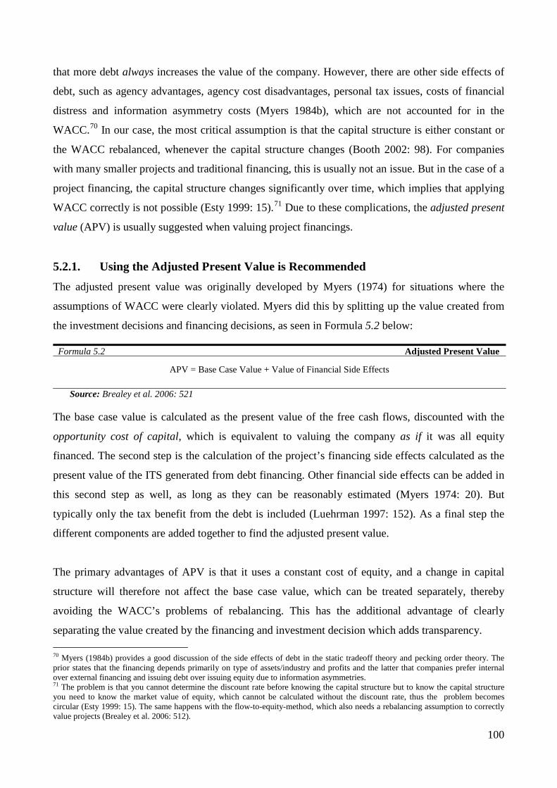
100

that more debt always increases the value of the company. However, there are other side effects of

debt, such as agency advantages, agency cost disadvantages, personal tax issues, costs of financial

distress and information asymmetry costs (Myers 1984b), which are not accounted for in the

WACC.70 In our case, the most critical assumption is that the capital structure is either constant or

the WACC rebalanced, whenever the capital structure changes (Booth 2002: 98). For companies

with many smaller projects and traditional financing, this is usually not an issue. But in the case of a

project financing, the capital structure changes significantly over time, which implies that applying

WACC correctly is not possible (Esty 1999: 15).71 Due to these complications, the adjusted present

value (APV) is usually suggested when valuing project financings.

5.2.1. Using the Adjusted Present Value is Recommended The adjusted present value was originally developed by Myers (1974) for situations where the

assumptions of WACC were clearly violated. Myers did this by splitting up the value created from

the investment decisions and financing decisions, as seen in Formula 5.2 below:

Formula 5.2 Adjusted Present Value

APV = Base Case Value + Value of Financial Side Effects


The base case value is calculated as the present value of the free cash flows, discounted with the

opportunity cost of capital, which is equivalent to valuing the company as if it was all equity

financed. The second step is the calculation of the project’s financing side effects calculated as the

present value of the ITS generated from debt financing. Other financial side effects can be added in

this second step as well, as long as they can be reasonably estimated (Myers 1974: 20). But

typically only the tax benefit from the debt is included (Luehrman 1997: 152). As a final step the

different components are added together to find the adjusted present value.

The primary advantages of APV is that it uses a constant cost of equity, and a change in capital

structure will therefore not affect the base case value, which can be treated separately, thereby

avoiding the WACC’s problems of rebalancing. This has the additional advantage of clearly

separating the value created by the financing and investment decision which adds transparency. 70 Myers (1984b) provides a good discussion of the side effects of debt in the static tradeoff theory and pecking order theory. The prior states that the financing depends primarily on type of assets/industry and profits and the latter that companies prefer internal over external financing and issuing debt over issuing equity due to information asymmetries. 71 The problem is that you cannot determine the discount rate before knowing the capital structure but to know the capital structure you need to know the market value of equity, which cannot be calculated without the discount rate, thus the problem becomes circular (Esty 1999: 15). The same happens with the flow-to-equity-method, which also needs a rebalancing assumption to correctly value projects (Brealey et al. 2006: 512).

101

However, the APV is no panacea. Most notably, it has problems with optimal debt ratios. This is

recognized by Myers (1974: 20) and thoroughly treated by Booth (2002: 99). In the case of a project

financing, this will not be an issue as an optimal debt ratio is not desired. Additionally APV, just

like WACC, does not properly account for financial distress or agency disadvantages, creating a

tendency to overvalue highly levered companies (Booth 2002: 102). Despite the shortcomings of

APV, it is in the case of project financing clearly superior to WACC and we therefore recommend it

in such cases. Based on this recommendation, we now turn to the calculation of the APV of the

operational phase.

5.3 Inclusion of the Interest Tax Shield in the Operational Phase To find the APV of the operational phase, we need to determine the cost of debt as well as the

standard terms for wind farm project finance in Denmark. Based on this information we can

calculate the value of the interest tax shield and find the APV of the operational phase.

5.3.1. Project Finance in Denmark In Denmark the two most active project finance banks are Ringkjøbing Landbobank and

VestjyskBANK with headquarters in western Jutland, an area with a long tradition for wind farm

construction. It is therefore likely that EE will finance their wind farms through one of these two

banks. In addition, Nordea also has a project finance office, although it is not as active in the Danish

wind farm market. The following information about project financing is provided through

interviews with the three banks. The interviews are summarized in Appendix 16.

The three banks all structure the financing of Danish wind farms in a similar way. The loans are

structured like an overdraft, where the entire cash flow is used to repay the debt. The debt has to be

fully repaid before the equity holders receive anything. The length of the loan thus varies according

to the principal, the production of the turbines and the cost of debt etc. Typically the banks’ target is

that the loan should be repaid approximately 8-13 years into the operational phase, which

determines the leverage of the individual project. This typically equals a leverage of approximately

65-90% of the initial investment. Based on previous experiences from their Italian and German

wind farms, EE aims for a leverage ratio of 80%. We have therefore chosen 80% as our initial

leverage ratio, which results in the loan being paid back in 7 years.

102

The cost of debt is in the three banks determined by the 6-month Copenhagen Interbank Offered

Rate (CIBOR) and the debt risk premium as seen in the formula below.

Formula 5.3 Cost of Debt

𝐫𝐝𝐞𝐛𝐭 = 𝐂𝐈𝐁𝐎𝐑 𝟔 + 𝐃𝐞𝐛𝐭 𝐑𝐢𝐬𝐤 𝐏𝐫𝐞𝐦𝐢𝐮𝐦

Source: Ringkøbing Landbobank, Vestjysk BANK and Nordea

The CIBOR is not equal to the risk-free rate since it includes a credit risk premium of lending to

commercial banks. The existence of such a credit risk premium is on international markets usually

expressed by the TED spread. This spread measures the London Interbank Offered Rate (LIBOR)

versus the 3-month T-bill interest rate (Cheung et al. 2010: 88), thereby expressing the difference

between the short term risk-free rate and the interbank rate.

However, the debt risk premium is more individual and typically depends on the individual project

specifications, the professionalism of the developer, the relationship to the bank etc.

5.3.1.1. The 6-month Copenhagen Interbank Offered Rate

The 6-month CIBOR is a daily reference rate based on the interest rates which banks lend and

borrow unsecured fund for in Copenhagen’s wholesale money market. Since CIBOR is a daily rate,

it is unlikely that it will remain constant through the life of the project and these fluctuations will

change the actual interest payments and thereby the ITS of the wind farm. It is therefore necessary

to identify a reasonable proxy for a longer period. This is technically the same problem as in chapter

4, when we discussed the risk-free rate used in the CAPM. There we pointed out that the

theoretically correct approach is to discount cash flows with a discount rate of a matching maturity.

In spite of this we saw that in practice a 10-year government bond was used to set the risk-free rate

for most corporate valuations, and that in general the discount rate is kept constant through the life

of the project. Based on a similar approach we have chosen to apply the 10-year Danish swap

reference rate, as a proxy for the long term CIBOR. This rate was 3.90 % (Nationalbanken) the 30th

of December 2009. We use the swap reference rate instead of a government bond as this can be

perceived as the long-term fixed-for-floating interbank rate (Finansraadet 2010).

5.3.1.2. The Debt Risk Premium

Besides the interbank rate, the cost of debt also contains a risk premium to adjust for the project’s

risk of default. This is typically denoted in basis points (BP). When estimating the debt risk

premium, we face many of the same issues as the ones from the beta estimation in section 4.2.3.2.

For example, the debt risk premium should reflect the individual project’s risk of default and not EE

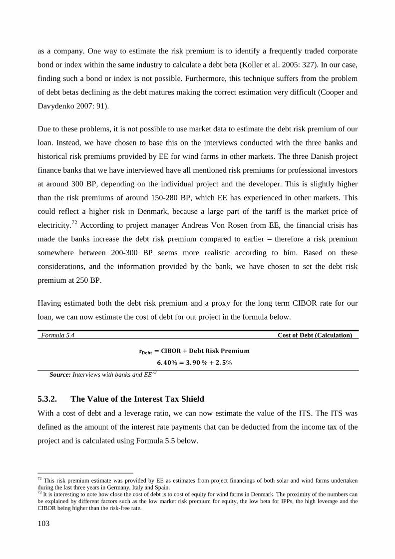
103

as a company. One way to estimate the risk premium is to identify a frequently traded corporate

bond or index within the same industry to calculate a debt beta (Koller et al. 2005: 327). In our case,

finding such a bond or index is not possible. Furthermore, this technique suffers from the problem

of debt betas declining as the debt matures making the correct estimation very difficult (Cooper and

Davydenko 2007: 91).

Due to these problems, it is not possible to use market data to estimate the debt risk premium of our

loan. Instead, we have chosen to base this on the interviews conducted with the three banks and

historical risk premiums provided by EE for wind farms in other markets. The three Danish project

finance banks that we have interviewed have all mentioned risk premiums for professional investors

at around 300 BP, depending on the individual project and the developer. This is slightly higher

than the risk premiums of around 150-280 BP, which EE has experienced in other markets. This

could reflect a higher risk in Denmark, because a large part of the tariff is the market price of

electricity.72 According to project manager Andreas Von Rosen from EE, the financial crisis has

made the banks increase the debt risk premium compared to earlier – therefore a risk premium

somewhere between 200-300 BP seems more realistic according to him. Based on these

considerations, and the information provided by the bank, we have chosen to set the debt risk

premium at 250 BP.

Having estimated both the debt risk premium and a proxy for the long term CIBOR rate for our

loan, we can now estimate the cost of debt for out project in the formula below.

Formula 5.4 Cost of Debt (Calculation)

𝐫𝐃𝐞𝐛𝐭 = 𝐂𝐈𝐁𝐎𝐑 + 𝐃𝐞𝐛𝐭 𝐑𝐢𝐬𝐤 𝐏𝐫𝐞𝐦𝐢𝐮𝐦

𝟔.𝟒𝟎% = 𝟑.𝟗𝟎 % + 𝟐.𝟓%

Source: Interviews with banks and EE73

5.3.2. The Value of the Interest Tax Shield With a cost of debt and a leverage ratio, we can now estimate the value of the ITS. The ITS was

defined as the amount of the interest rate payments that can be deducted from the income tax of the

project and is calculated using Formula 5.5 below.

72 This risk premium estimate was provided by EE as estimates from project financings of both solar and wind farms undertaken during the last three years in Germany, Italy and Spain. 73 It is interesting to note how close the cost of debt is to cost of equity for wind farms in Denmark. The proximity of the numbers can be explained by different factors such as the low market risk premium for equity, the low beta for IPPs, the high leverage and the CIBOR being higher than the risk-free rate.

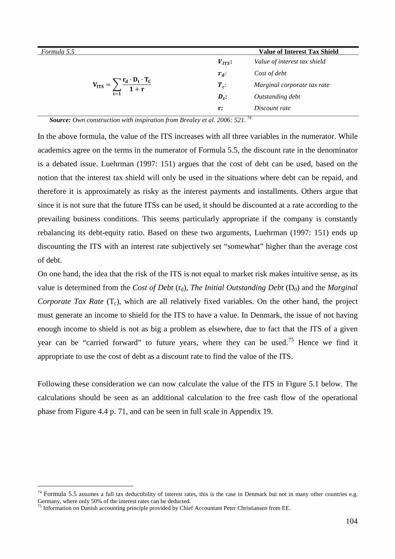
104

Formula 5.5 Value of Interest Tax Shield

𝐕𝐈𝐓𝐒 = �𝐫𝐝 ∙ 𝐃𝐭 ∙ 𝐓𝐂𝟏 + 𝐫

𝐭=𝟏

𝑽𝑰𝑻𝑺: Value of interest tax shield

𝒓𝒅: Cost of debt

𝑻𝒄: Marginal corporate tax rate

𝑫𝒕: Outstanding debt

r: Discount rate

Source: Own construction with inspiration from Brealey et al. 2006: 521. 74

In the above formula, the value of the ITS increases with all three variables in the numerator. While

academics agree on the terms in the numerator of Formula 5.5, the discount rate in the denominator

is a debated issue. Luehrman (1997: 151) argues that the cost of debt can be used, based on the

notion that the interest tax shield will only be used in the situations where debt can be repaid, and

therefore it is approximately as risky as the interest payments and installments. Others argue that

since it is not sure that the future ITSs can be used, it should be discounted at a rate according to the

prevailing business conditions. This seems particularly appropriate if the company is constantly

rebalancing its debt-equity ratio. Based on these two arguments, Luehrman (1997: 151) ends up

discounting the ITS with an interest rate subjectively set “somewhat” higher than the average cost

of debt.

On one hand, the idea that the risk of the ITS is not equal to market risk makes intuitive sense, as its

value is determined from the Cost of Debt (rd), The Initial Outstanding Debt (D0) and the Marginal

Corporate Tax Rate (Tc), which are all relatively fixed variables. On the other hand, the project

must generate an income to shield for the ITS to have a value. In Denmark, the issue of not having

enough income to shield is not as big a problem as elsewhere, due to fact that the ITS of a given

year can be “carried forward” to future years, where they can be used.75 Hence we find it

appropriate to use the cost of debt as a discount rate to find the value of the ITS.

Following these consideration we can now calculate the value of the ITS in Figure 5.1 below. The

calculations should be seen as an additional calculation to the free cash flow of the operational

phase from Figure 4.4 p. 71, and can be seen in full scale in Appendix 19.

74 Formula 5.5 assumes a full tax deductibility of interest rates, this is the case in Denmark but not in many other countries e.g. Germany, where only 50% of the interest rates can be deducted. 75 Information on Danish accounting principle provided by Chief Accountant Peter Christiansen from EE.

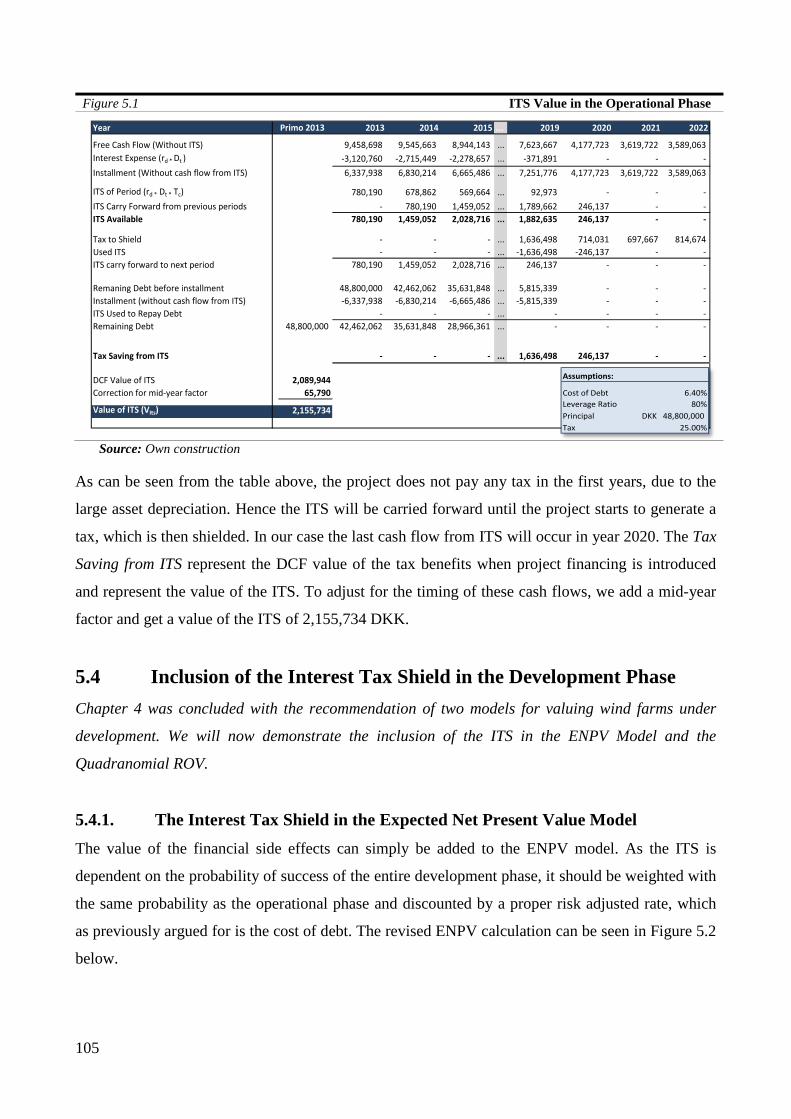
105

Figure 5.1 ITS Value in the Operational Phase


As can be seen from the table above, the project does not pay any tax in the first years, due to the

large asset depreciation. Hence the ITS will be carried forward until the project starts to generate a

tax, which is then shielded. In our case the last cash flow from ITS will occur in year 2020. The Tax

Saving from ITS represent the DCF value of the tax benefits when project financing is introduced

and represent the value of the ITS. To adjust for the timing of these cash flows, we add a mid-year

factor and get a value of the ITS of 2,155,734 DKK.

5.4 Inclusion of the Interest Tax Shield in the Development Phase Chapter 4 was concluded with the recommendation of two models for valuing wind farms under

development. We will now demonstrate the inclusion of the ITS in the ENPV Model and the

Quadranomial ROV.

5.4.1. The Interest Tax Shield in the Expected Net Present Value Model The value of the financial side effects can simply be added to the ENPV model. As the ITS is

dependent on the probability of success of the entire development phase, it should be weighted with

the same probability as the operational phase and discounted by a proper risk adjusted rate, which

as previously argued for is the cost of debt. The revised ENPV calculation can be seen in Figure 5.2

below.

Year Primo 2013 2013 2014 2015 ... 2019 2020 2021 2022

Free Cash Flow (Without ITS) 9,458,698 9,545,663 8,944,143 ... 7,623,667 4,177,723 3,619,722 3,589,063 Interest Expense (rd * Dt ) -3,120,760 -2,715,449 -2,278,657 ... -371,891 - - - Installment (Without cash flow from ITS) 6,337,938 6,830,214 6,665,486 ... 7,251,776 4,177,723 3,619,722 3,589,063

ITS of Period (rd * Dt * Tc) 780,190 678,862 569,664 ... 92,973 - - - ITS Carry Forward from previous periods - 780,190 1,459,052 ... 1,789,662 246,137 - - ITS Available 780,190 1,459,052 2,028,716 ... 1,882,635 246,137 - -

Tax to Shield - - - ... 1,636,498 714,031 697,667 814,674 Used ITS - - - ... -1,636,498 -246,137 - - ITS carry forward to next period 780,190 1,459,052 2,028,716 ... 246,137 - - -

Remaning Debt before installment 48,800,000 42,462,062 35,631,848 ... 5,815,339 - - - Installment (without cash flow from ITS) -6,337,938 -6,830,214 -6,665,486 ... -5,815,339 - - - ITS Used to Repay Debt - - - ... - - - - Remaining Debt 48,800,000 42,462,062 35,631,848 28,966,361 ... - - - -

Tax Saving from ITS - - - ... 1,636,498 246,137 - -

DCF Value of ITS 2,089,944Correction for mid-year factor 65,790

Value of ITS (VIts) 2,155,734

Assumptions:

Cost of Debt 6.40%Leverage Ratio 80%Principal 48,800,000DKK Tax 25.00%

106

Figure 5.2 ENPV Calculation Including Debt


5.4.2. The Interest Tax Shield in the Real Options Valuation The issue of financing side effects is treated quite extensively in the standard DCF literature as

opposed to the situation in the ROV literature. Instead, the ROV literature typically assumes a

Miller-Modgliani world with financing being irrelevant (Bulan 2005: 272). The few exceptions we

have found do not treat it for projects under development, but instead for the interaction between

operational production flexibility and debt capacity (Mauer and Triantis 1994), optimal investment

structure and capital structure (Copeland WP: 1), or leveraged buy-outs of a company (Baldi 2005:

64). Other more practical texts such Copeland and Antikarov (2003), Mun (2002) and Shockley

(2007) discount the operational cash flows using a constant WACC – thereby implicitly assuming a

constant debt-equity ratio of the underlying asset. Based on these initial considerations, the question

is how the value of ITS should be accounted for in our ROV of a wind farm under development.

Before addressing this issue it is necessary with an improved understanding of the ITS’s

relationship to the different market states.

The value of the ITS will not be directly correlated with the market state as its value depends on

factors such as the amount borrowed, whether the loan can be serviced and the pace at which it is

repaid. Although such factors will to some extent be correlated to the market state, it is clear from

Figure 5.3 below, where the electricity price is set as a proxy for the market development, that the

value of the ITS does not vary much with different electricity prices.

Stage Time Prob. Stage

Probability of Construction Cash Flow (t) PV (t=0) Probability

Weighted PVStage 1: Analysis and Pre-approval 0 50% 100% -100,000 -100,000 -100,000 Stage 2: VVM & Final Approval 0.5 50% 50% -500,000 -491,189 -245,594 Stage 3: Complaints and Compensation 1.5 80% 25% -500,000 -474,029 -118,507 Stage 4: Construction 2.5 100% 20% -61,000,000 -55,811,136 -11,162,227 Value of Operational Phase 3 0% 20% 70,479,996 57,827,251 11,565,450Value of ITS 3 - 20% 2,155,734 1,789,912 357,982

ENPV (Including Debt) 297,104

107

Figure 5.3 Change in ITS Value from different Electricity Prices76


The reason that the ITS is not exactly constant is because at the low electricity prices, the ITS is

used very late in the operational phase, partly due to the asset depreciation, leading to a lower

present value of the ITS. The high prices lead to the loan being repaid faster, resulting in fewer

interest payments, thereby reducing the value of the ITS. These relationships demonstrate both the

complexity and the stability of the ITS value in relation to the market state. At the same time, it

could be argued that a change in the market state could change the leverage ratio of the project, as

banks are willing to lend more money to a good project. If an improved market state leads to a

higher leverage ratio, the value of the ITS will increase ceteris paribus. Furthermore, an improved

market state is likely to lead to a lower risk premium as the default risk is reduced creating a lower

ITS, as shown in the two graphs in the figure below.

Figure 5.4 ITS Value Given Different Leverage Ratios and Debt Risk Premiums


76 The electricity price in the figure represents the price when the wind farm is constructed and is fixed for all 20-years of the operational phase. This is supposed to demonstrate the fact that the value of the tax shield is relatively constant. It should be noted, however, that in the case of very low electricity prices the project will default, this means that the value of the tax shield is reduced dramatically. However, in such cases the project would have been abandoned during development and these states can therefore be disregarded.

DKK -

DKK 500.000

DKK 1.000.000

DKK 1.500.000

DKK 2.000.000

DKK 2.500.000

DKK 3.000.000

0,27 0,29 0,31 0,33 0,35 0,37 0,39 0,41 0,43 0,45 0,47 0,49

Valu

e of

ITS

Electricity Price (DKK/kWh)

Risk Premium

DKK -

DKK 500,000

DKK 1,000,000

DKK 1,500,000

DKK 2,000,000

DKK 2,500,000

DKK 3,000,000

Valu

e of

ITS

Leverage Ratio

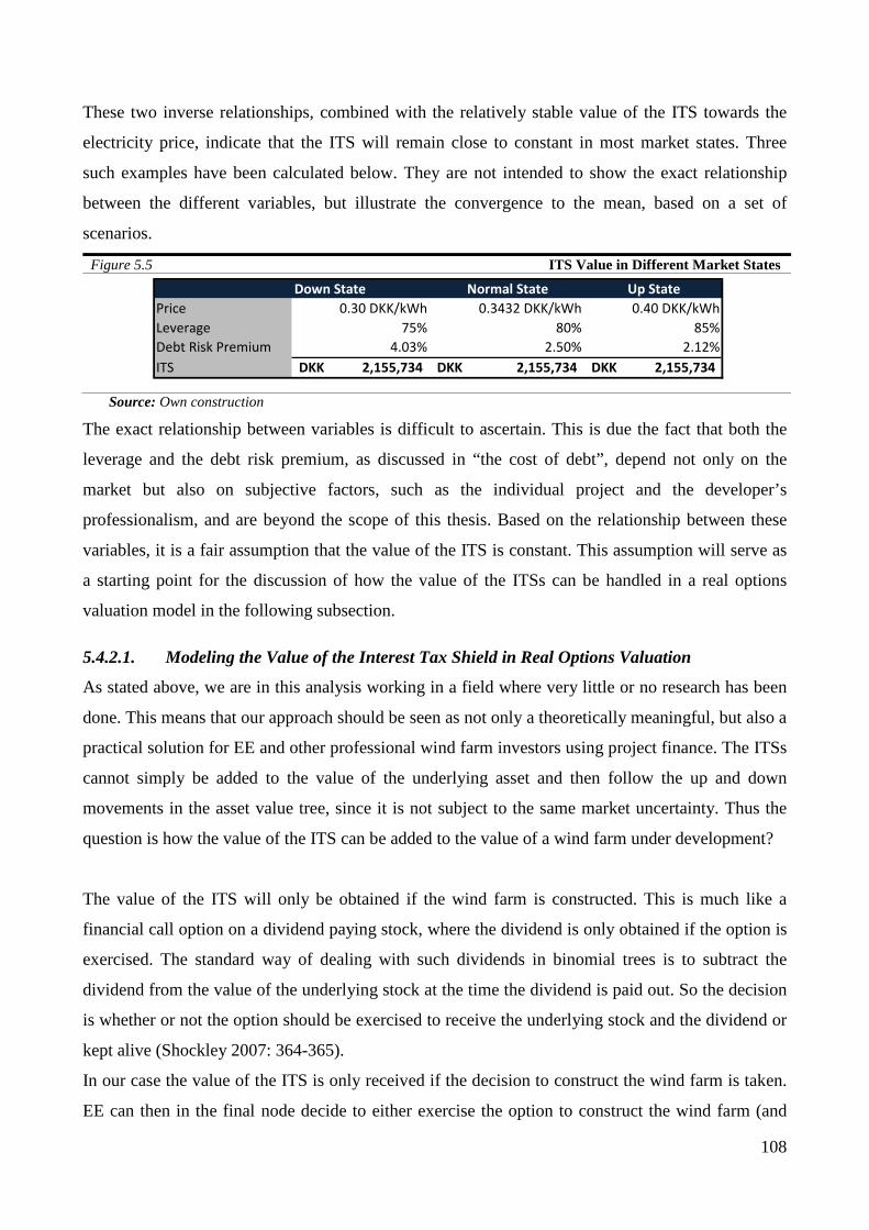
108

These two inverse relationships, combined with the relatively stable value of the ITS towards the

electricity price, indicate that the ITS will remain close to constant in most market states. Three

such examples have been calculated below. They are not intended to show the exact relationship

between the different variables, but illustrate the convergence to the mean, based on a set of

scenarios.

Figure 5.5 ITS Value in Different Market States


The exact relationship between variables is difficult to ascertain. This is due the fact that both the

leverage and the debt risk premium, as discussed in “the cost of debt”, depend not only on the

market but also on subjective factors, such as the individual project and the developer’s

professionalism, and are beyond the scope of this thesis. Based on the relationship between these

variables, it is a fair assumption that the value of the ITS is constant. This assumption will serve as

a starting point for the discussion of how the value of the ITSs can be handled in a real options

valuation model in the following subsection.

5.4.2.1. Modeling the Value of the Interest Tax Shield in Real Options Valuation

As stated above, we are in this analysis working in a field where very little or no research has been

done. This means that our approach should be seen as not only a theoretically meaningful, but also a

practical solution for EE and other professional wind farm investors using project finance. The ITSs

cannot simply be added to the value of the underlying asset and then follow the up and down

movements in the asset value tree, since it is not subject to the same market uncertainty. Thus the

question is how the value of the ITS can be added to the value of a wind farm under development?

The value of the ITS will only be obtained if the wind farm is constructed. This is much like a

financial call option on a dividend paying stock, where the dividend is only obtained if the option is

exercised. The standard way of dealing with such dividends in binomial trees is to subtract the

dividend from the value of the underlying stock at the time the dividend is paid out. So the decision

is whether or not the option should be exercised to receive the underlying stock and the dividend or

kept alive (Shockley 2007: 364-365).

In our case the value of the ITS is only received if the decision to construct the wind farm is taken.

EE can then in the final node decide to either exercise the option to construct the wind farm (and

Down State Normal State Up StatePrice 0.30 DKK/kWh 0.3432 DKK/kWh 0.40 DKK/kWhLeverage 75% 80% 85%Debt Risk Premium 4.03% 2.50% 2.12%ITS 2,155,734DKK 2,155,734DKK 2,155,734DKK

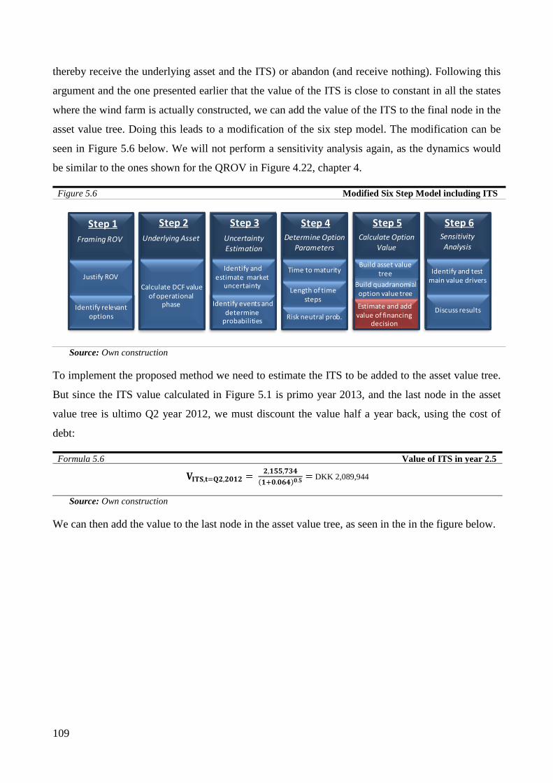
109

thereby receive the underlying asset and the ITS) or abandon (and receive nothing). Following this

argument and the one presented earlier that the value of the ITS is close to constant in all the states

where the wind farm is actually constructed, we can add the value of the ITS to the final node in the

asset value tree. Doing this leads to a modification of the six step model. The modification can be

seen in Figure 5.6 below. We will not perform a sensitivity analysis again, as the dynamics would

be similar to the ones shown for the QROV in Figure 4.22, chapter 4.

Figure 5.6 Modified Six Step Model including ITS


To implement the proposed method we need to estimate the ITS to be added to the asset value tree.

But since the ITS value calculated in Figure 5.1 is primo year 2013, and the last node in the asset

value tree is ultimo Q2 year 2012, we must discount the value half a year back, using the cost of

debt:

Formula 5.6 Value of ITS in year 2.5

𝐕𝐈𝐓𝐒,𝐭=𝐐𝟐,𝟐𝟎𝟏𝟐 = 𝟐,𝟏𝟓𝟓,𝟕𝟑𝟒(𝟏+𝟎.𝟎𝟔𝟒)𝟎.𝟓 = DKK 2,089,944


We can then add the value to the last node in the asset value tree, as seen in the in the figure below.

Sensitivity Analysis

Step 1Framing ROV

Justify ROV




phase



Identify events and determine

probabilities


uncertainty

Step 4Determine Option

Parameters

Time to maturity


Risk neutral prob.



Value


Estimate and add value of financing

decision

Build asset valuetree

Step 6


Discuss results

SensitivityAnalysis

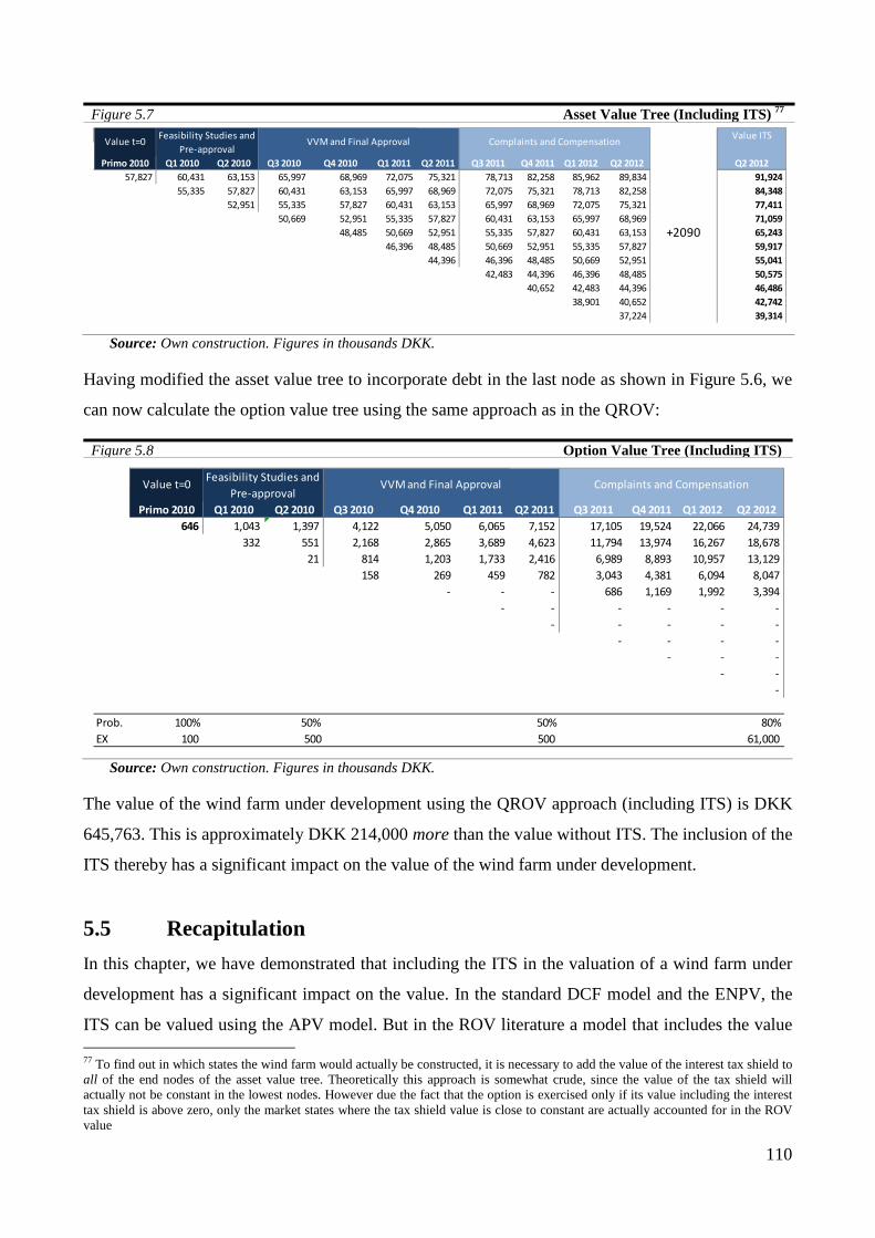
110

Figure 5.7 Asset Value Tree (Including ITS) 77


Having modified the asset value tree to incorporate debt in the last node as shown in Figure 5.6, we

can now calculate the option value tree using the same approach as in the QROV:

Figure 5.8 Option Value Tree (Including ITS)


The value of the wind farm under development using the QROV approach (including ITS) is DKK

645,763. This is approximately DKK 214,000 more than the value without ITS. The inclusion of the

ITS thereby has a significant impact on the value of the wind farm under development.

5.5 Recapitulation In this chapter, we have demonstrated that including the ITS in the valuation of a wind farm under

development has a significant impact on the value. In the standard DCF model and the ENPV, the

ITS can be valued using the APV model. But in the ROV literature a model that includes the value 77 To find out in which states the wind farm would actually be constructed, it is necessary to add the value of the interest tax shield to all of the end nodes of the asset value tree. Theoretically this approach is somewhat crude, since the value of the tax shield will actually not be constant in the lowest nodes. However due the fact that the option is exercised only if its value including the interest tax shield is above zero, only the market states where the tax shield value is close to constant are actually accounted for in the ROV value

Value ITS

Primo 2010 Q1 2010 Q2 2010 Q3 2010 Q4 2010 Q1 2011 Q2 2011 Q3 2011 Q4 2011 Q1 2012 Q2 2012 Q2 201257,827 60,431 63,153 65,997 68,969 72,075 75,321 78,713 82,258 85,962 89,834 91,924

55,335 57,827 60,431 63,153 65,997 68,969 72,075 75,321 78,713 82,258 84,348 52,951 55,335 57,827 60,431 63,153 65,997 68,969 72,075 75,321 77,411

50,669 52,951 55,335 57,827 60,431 63,153 65,997 68,969 71,059 48,485 50,669 52,951 55,335 57,827 60,431 63,153 65,243

46,396 48,485 50,669 52,951 55,335 57,827 59,917 44,396 46,396 48,485 50,669 52,951 55,041

42,483 44,396 46,396 48,485 50,575 40,652 42,483 44,396 46,486

38,901 40,652 42,742 37,224 39,314



+2090

Primo 2010 Q1 2010 Q2 2010 Q3 2010 Q4 2010 Q1 2011 Q2 2011 Q3 2011 Q4 2011 Q1 2012 Q2 2012646 1,043 1,397 4,122 5,050 6,065 7,152 17,105 19,524 22,066 24,739

332 551 2,168 2,865 3,689 4,623 11,794 13,974 16,267 18,678 21 814 1,203 1,733 2,416 6,989 8,893 10,957 13,129

158 269 459 782 3,043 4,381 6,094 8,047 - - - 686 1,169 1,992 3,394

- - - - - - - - - - -

- - - - - - -

- - -

Prob. 100% 100% 50% 100% 100% 100% 50% 100% 100% 100% 80%EX 100 500 500 61,000



111

of the ITS for projects under development does not seem to exist. However, as we have argued in

this chapter, it is actually possible to add the value of the ITS in the operational phase to the value

of a wind farm under development. Our approach thereby makes it possible for companies like EE

to use ROV – also for wind farms that are project financed. The valuation thereby goes one step

further than previous attempts to use ROV models for wind farms under development. We claim

that this approach provides a model with a higher relevance and a better valuation of wind farms

under development.

We have throughout chapter 4 and 5 gradually developed our six step model to be able to create a

ROV model which could actually be used by EE. In addition to developing and refining this model,

we have also wanted to highlight the usability criterion of particularly ROV. This criterion has been

discussed by performing the actual calculations and estimations. Doing this it has been

demonstrated that the estimations are uncertain and that all of the models move away from their

theoretical ideal when the valuations are undertaken in practice. It is therefore important for

practitioners to understand the assumptions of the models – in ability to implement them and

interpret their results correctly. The relevant notion thus becomes what model assists this process in

the most appropriate manner. This is also acknowledged by financial “geniuses” like Robert C.

Merton: “The mathematics of financial models can be applied precisely, but the models are not at

all precise in their application to the complex real world … the models should be applied in

practice only tentatively, with careful assessment of their limitations in each application”.78

However, the notion is just as often forgotten, once “the heat is on”. Merton himself was part of the

Long-Term Capital Management crash in 1998, only a year after receiving the Nobel Prize in

economics with the above quote. It is such facts that underline how important the usability criterion

is and make it relevant to question the appropriateness of very advanced models within corporate

finance.

78 Quote from Merton’s Nobel Prize Speech in Miller and Park (128: 105).

112

6 Conclusion & Perspectives We have discussed and compared different valuation models and their application to wind farms

under development in order to achieve the two objectives of the thesis. The first objective was to

investigate if a ROV model could be developed to improve the valuation of wind farms under

development in comparison to DCF based models. The second objective was to investigate the

practical usability of such a model. We have demonstrated that both objectives are achievable. We

will here discuss the main findings and end by putting them into perspective.

6.1 A ROV Model for Wind Farms under Development In the thesis it is demonstrated that it is both practically and theoretically possible to develop a ROV

model of wind farms under development. This was done using the binomial model, found in the

practical ROV literature, as a starting point. In order to use this model, we set up six steps for a

binomial real options valuation and throughout the thesis, we gradually modified the model to

address the relevant issues when valuing a wind farm under development. The modification

consisted of the inclusion of the failure events during the development phase using the

quadranomial approach, and the inclusion of the added value created by the financing decision. The

modified version of the six step model can be seen in Figure 6.1 below, and represents our

suggestion of a valuation model that can improve the valuation of a wind farm under development

in Denmark.

Figure 6.1 Six Step Model for ROV of a Wind Farm Under Development


The first step is the framing of the real options valuation, which included a discussion of the

relevant option and a justification of the more complex ROV approach. The second step consists of

the identification and valuation of the underlying asset, in our case this underlying asset is the value

of the operational phase. The third step includes the estimation of the market uncertainty

represented by the volatility of the underlying asset as well as the events, such as a failure during

Sensitivity Analysis

Step 1Framing ROV

Justify ROV




phase



Identify events and determine

probabilities


uncertainty

Step 4Determine Option

Parameters

Time to maturity


Risk neutral prob.



Value


Estimate and add value of financing

decision

Build asset valuetree

Step 6


Discuss results

SensitivityAnalysis

113

the development phase, and the probability of these. The fourth step is to determine the specific

option parameters, which are both used in the binomial model and the quadranomial approach. In

step five, the four previous steps are used to construct the asset value tree and option value tree to

calculate the option value. Having performed the valuation, the sixth step discussed the results using

a sensitivity analysis.

Based on this model we were able to calculate a superior value for a wind farm under development

than the DCF-based alternative, the ENPV, as seen in Table 6.1 below.

Table 6.1 Value of a Danish Wind Farm under Development

Model Without Debt With Debt

ENPV -60,879 497,104

Quadranomial ROV 431,289 645,763


The improved result from the ROV model compared to ENPV comes from its ability to include the

market uncertainty and the flexibility that European Energy has during the development phase. It is

from the ability to capture the value of this flexibility that ROV bridges the gap between finance

and strategic decision making. The fact that ROV bridges the gap means that it not only improves

the financial valuation, but it also provides a better framework for managers than DCF models for

evaluating strategic decisions, as it creates a better “lens” for viewing different investment

proposals.

6.2 The Usability of ROV Models It should be clear from the thesis that any financial valuation requires both challenging and

thorough analysis of a long range of factors. Therefore, we defined analysis of the usability criterion

as one of the main objective in our thesis – an objective that is particularly important for ROV due

to its lack of acceptance among practitioners.

In the discussion of the different models we saw that despite the standard DCF model generally

being praised as intuitive and easy, the actual estimations of the input to the model are not simple.

In relation to usability, we also discussed the often heard critique that ROV’s assumptions are

unrealistic. Here we saw that the necessary assumptions are not stronger than the ones found in

many DCF valuations – and as such the critique is unfair. At the same time we conceded that ROV

suffers from several drawbacks with regard to usability. Especially the disagreement between

academics concerning the volatility estimation is problematic. Based on the current literature, we

114

recommend using the volatility of the commodity related to the underlying asset as an expression

for the market uncertainty of the project, when possible. This approach is often found in the

literature and furthermore has the large advantage of providing an intuitive and transparent

volatility estimate for practitioners. Using a commodity as a proxy for the volatility and

acknowledging that the assumptions of the DCF models are also strong, seems like a step in the

right direction of getting practitioners to accept real options valuation.

It is based on the recognition of such usability issues and the significant uncertainty of the

estimates, used in the valuation models that we have chosen to compare many of the estimates with

different peers. Such comparison and discussion clearly demonstrates that valuations are no exact

science. It is therefore relevant to discuss whether it is actually meaningful to develop very

advanced models to perform valuations, given the significant uncertainty of these estimates. This

critique explains the skepticism found among practitioners towards advanced valuation models.

What is important to reemphasize is the fact that while it can be discussed if the ROV actually

provides a more precise financial valuation, it clearly provides a better understanding of the

uncertainties and options of a project and is therefore able to deliver valuable managerial insights.

6.3 Market Uncertainty Revisited In spite of our general recommendation of ROV, we have also noted that it cannot be applied to any

situation, as it requires the presence of a contingent future decision and a certain level of uncertainty

to make sense. We have argued throughout this thesis that this is the case for wind farms under

development. These arguments can be challenged.

First, it can be questioned whether or not wind farms under development are exposed to the high

market uncertainty which we use. This question is raised based on the considerable political

attention which the renewable energy sector has been receiving the last years. From this it can be

questioned what would happen if electricity prices were to rise or fall considerably during the

development phase. In such a situation it is not unthinkable that the subsidy system would change to

adjust for the price change. The idea of such an adjustment is based on the idea that most

governments will not want wind farm investments to be too good or too poor investments – but to

earn a “reasonable return”.79 Since the subsidy is not fixed until the wind farm has been

commissioned, it is possible that the market uncertainty to a large extent would be offset by a

change in the subsidy system. Such a possibility has not been accounted for in any of the valuation

79 Such a target of governments can for example be observed in a recent Emerging Energy Research study (2010: 8) that calculates internal-rate-of-returns on five different offshore markets, obtaining results between 8 to 10%, and thereby suggesting some sort of predefined “reasonable” return on this type of investments.

115

models – based on the notion that it represents an “immeasurable” uncertainty. This critique will

only apply as long as wind farms are dependent on government subsidies – and as these subsidies

most likely become smaller in the upcoming years – ROV will become even more relevant.

A second question that can be raised is whether a company will actually exercise its real options, as

the options financial value is usually not the only decision parameter. This question, along with

ROV’s influence on strategy, is discussed in the following section.

6.4 Perspectives Throughout the thesis there has been a focus on the financial assumptions of the models. We end

the thesis by expanding this focus and discuss ROV in a broader organizational context,

highlighting ROV’s interactions with corporate governance and strategy theory.

6.4.1. Managing Real Options One of the key differences between managing financial options and real options (as seen previously

in Table 3.6) is the economic agent. In financial options, it is an investor who holds the right to

exercise the option. Whereas for real options, it is an employee who is the decision maker and holds

the right to exercise the option.80 This challenges ROV in the sense that where the agent holding a

financial option can be assumed to act rationally, this assumption can be questioned with regard to

the corporate decision maker. Questions can thus be raised about whether the options will be

exercised and if managers will actually adapt the real options way of thinking when choosing

between projects. The problems discussed here are related to principal-agent problem discussed in

economic literature (Jensen and Meckling 1976: 308).

Financial options will only be exercised if this leads to a profit for the investor, otherwise the option

will be left unexercised and the price paid for the option will represent a loss. Such a rational

calculating behavior might not always be present for real options exercise. It is possible that a

decision maker, despite a negative market development, will continue the development of a wind

farm and thus exercise the option to continue, even in a situation where he should not do so. Such

“irrational” behavior could be based on emotional ties to a project. This could be the case for EE,

based on a desire of as a Danish company to be present in Denmark. Alternatively, it could be due

to the fact that they already spent a lot of time and effort. The idea that decision makers undertake

negative NPV investment due to personal interests is acknowledged in corporate finance literature.

This can represent a decision maker’s desire to increase the size of the company (empire-building)

80 Some very large investment decisions might need to be approved by a shareholders’ meeting.

116

or can also be an entrenching investment, i.e. that managers prefer to invest in projects which

require their skills (Brealey et al. 2006: 304). Such potential principal-agent conflicts challenge the

result obtained in the real option valuation (Philippe 2005: 130).

Another problem is found in Miller and Park (2002: 128) with an example of two projects with the

same expected return, but differences in volatility, where ROV suggests that the more volatile

project should be chosen. This leads to the question of whether or not the decision maker will

actually choose the more volatile project. This decision is likely to depend on the way the decision

maker is incentivized as he is likely to make choices to his own benefit. To avoid irrational

decisions, an alignment of the decision makers’ and the shareholders’ incentives is thus necessary

(Philippe 2005: 134). In the example, the decision maker is unlikely to choose the higher risk

project, unless he can gain from the upside and not only risk his job due to the down side.

This corporate governance perspective on real options turns the critique of the standard DCF model

upside down. Where the DCF model is criticized for assuming a passive holding of assets, the ROV

model can be criticized for assuming an active holding of assets with rational decision making.

6.4.2. Real Options and Strategy Revisited It has been argued in the thesis that a large part of the value from the ROV approach is its strategic

value, as it forces decision makers to think about the different decisions in a project. It is interesting

to think this deeper into the strategy process of companies, because the approach highlights that

projects are continuously changing, and there is a value in being able to capture this. Such a

flexibility dimension is lacking in much corporate strategy thinking, which akin to standard DCF

models all too often emphasizes static decisions. This static view on strategy is reflected in the

work of classical strategy scholars such as Porter (1979 and 1996). The general idea in Porter’s

work is strategy as creating and sustaining a competitive advantage based on a unique position on

the market or a fit of activities. Such a view of strategy can be challenged by ROV, leading to a

definition of strategy where the focus should be on a company’s ability to create and capture

flexibility. This is in line with what Mintzberg and Waters (1985: 258) call an “emerging strategy”.

This view on strategy is more preoccupied with creating room for flexibility by opening up the

strategy-making process for new opportunities (Mintzberg 1994: 108). This kind of view on

strategy thereby matches with ROV, as it also focuses on remaining open towards uncertainty in

order to be able to react to and create new opportunities. In this perspective, it can be said that it is

not finance which needs to approach strategy but instead both disciplines that need to open up.

117

7 References

• Amram, M. & Kulatilaka, N. (1999). “Real Options: Managing Strategic Investment in an Uncertain World”. Boston: Harvard Business School Press.

• Andersen, I. (2002). “Den skinbarlige virkelighed - om Vidensproduktion Indenfor Samfundsvidenskaberne” (2nd edition). Forlaget Samfundslitteratur.

• Arnold, T. & Shockley, R.L. (2003). “Corporate Finance and the Foundations of Value Maximization”. Journal of Applied Corporate Finance, (15.2):82-88.

• Baldi. F (2005). “Valuing a Leveraged Buyout: Expansion of the Adjusted Present Value by Means of Real Options Analysis”. Journal of Private Equity, Fall: 64-81.

• Bessis, J. (2002). “Risk Management in Banking” (2nd Edition). John Wiley and Sons Inc. • Black, F. (1975). “The Pricing of Commodity Contracts”. Journal of Financial Economics, 3:

167-179. • Black, F. & Scholes, M. (1973). “The Pricing of Options and Corporate Liabilities”. Journal of

Political Economy, 81(3): 637. • Blanco, C.; Choi, S. & Soronow, D. (2001). “Energy Price Processes Used for Derivatives

Pricing & Risk Management”. Commodities Now: 74-86. • Blanco, C. & Soronow, D. (2001a). “Mean Reverting Processes – Energy Price Processes Used

for Derivatives Pricing & Risk Management”. Commodities Now: 68-72. • Blanco, C. & Soronow, D. (2001b). “Jump Diffusion Processes – Energy Price Processes Used

for Derivatives Pricing & Risk Management”. Commodities Now: 83-87. • Booth, L. (2002). "Finding Value Where None Exists: Pitfalls in Using Adjusted Present Value".

Journal of Applied Corporate Finance, (15.1):95-104. • Borison, A. (2005). “Real Options Analysis: Where Are the Emperor’s Clothes?” Journal of

Applied Corporate Finance, (17.2):17-31. • Brandão, L.E.; Dyer, J.S. & Hahn, W.J. (2005). “Using Binomial Decision Trees to Solve

Real Options Valuation Problems”. Decision Analysis, 2(2): 69-88. • Brealey, R.A.; Cooper, I.A. & Habib, M.A. (1996). “Using Project Finance to Fund

Infrastructure Investments”. Journal of Applied Corporate Finance, Fall, (9.3): 25-38. • Brealey, R. A.; Myers, S. C., & Allen, F. (2006). “Principles of Corporate Finance” (8th

edition). McGraw-Hill. • Bulan, L. (2005). “Real Options, Irreversible Investment and Firm Uncertainty: New Evidence

from U.S. Firms”. Review of Financial Economics, 14: 255-279. • Bøckman, T.; Fleten, S.; Juliussen, E.: Håvard, J.L. & Revdal, I. (2007). "Investment Timing

and Optimal Capacity Choice for Small Hydropower Projects". European Journal of Operational Research, (190): 255-267.

• Børsen, Jakob Skouboe (2009). “Økonomien i Havmøller Er Under Stort Pres”. 29-10-2009. • Chemmanur, T. & John, K. (1992). “Optimal Incorporation, Structure of Debt Contracts, and

Limited-Recourse Project Financing”. Journal of Financial Intermediation, 5: 372–408. • Cheung, W.; Fung, S. & Tsai, S. (2010). "Global Capital Market Interdependence and Spillover

Effect of Credit Risk: Evidence from the 2007-2009 Global Financial Crisis". Applied Financial Economics, 20: 85–103.

• Christiansen, J. & B. Lystbæk (1994). “Afkast og Risiko På Aktier og Obligationer 1915-1993”. Finans/Invest: 10-13.

• Cooper, I. & Davydenko, S. (1997). “Estimating the Cost of Risky Debt”. Journal of Applied Corporate Finance, (19.3): 90-96.

118

• Copeland, T. “The Firm as a Three-Layer Cake – Optimal Investment and Financial Structure”. Working Paper, MIT Sloan School of Business.

• Copeland, T., & Antikarov, V. (2003). “Real Options: A Practitioner's Guide”. Thomson: TEXERE.

• Copeland, T.; Koller, T. & Murrin, J. (1994). “Valuation: Measuring and Managing the Value of Companies” (2nd Edition). John Wiley & Sons Inc.

• Cox, J. C.; Ross, S. & Rubinstein, M. (1979). “Option Pricing: A Simplified Approach”. Journal of Financial Economics, 7: 229-263.

• Dam-Rasmussen, C. & Würtz, C. (2003). ”The Valuation Process for Drug Development Projects”. Master Thesis, Copenhagen Business School.

• Danmarks Nationalbank. Databases. http://nationalbanken.statistikbank.dk. • Dimson, E.; Marsh, P. & Staunton, M. (2002). “Triumph of the Optimists: 101 years of Global

Investment Returns”. University Press of California. • Dixit, A. & Pindyck, R. (1994). “Investment under Uncertainty”. Princeton University Press. • dkvind (2009a). Danish Wind Turbine Owners’ Association, Faktablad Ø5, “Afregningsregler

for Vindmøller”. Available: www.dkvind.dk. • dkvind (2009b). Danish Wind Turbine Owners’ Association, Faktablad T3, “Indpasning af

Vindkraft i Elsystemet”. Available: www.dkvind.dk. • Dunlop, J. (2004). “Modern Portfolio Theory Meets Wind Farms”. Journal of Private Equity,

Spring: 83-95. • Dykes, K. & Neufville, R. (2008). “Real Options for a Wind Farm in Wapakoneta, Ohio:

Incorporating Uncertainty into Economic Feasibility Studies for Community Wind”. Paper submitted for the World Wind Energy Conference of 2008, Kingston, Ontario.

• Elton, E.; Gruber, J.; Brown, S. & Goetzmann, W. (2007). “Modern Portfolio Theory and Investment Analysis” (7th Edition). John Wiley & Sons Inc.

• Emerging Energy Research, Sala de Vedruna, E.; Mühlenbach, M. & Frølunde, S. (2009a). “Europe Wind Plant Ownership Rankings by Country, 2008: Top Ten Markets.”

• Emerging Energy Research (2009b). “Europe Market Study”. • Emerging Energy Research, Gautier, V. & Sala de Vedruna, E. (2010). “Europe Offshore

Wind Power Country Attractiveness Analysis”. • Energinet.dk, Link 1 (2009). http://www.energinet.dk/da/menu/Nyheder/-

Nyhedsartikler/Energinet.dk+er+i+gang+med+at+lægge+højspændingskabel+på+Østfyn.htm. • Energinet.dk, link 2 (2009). http://www.energinet.dk/NR/exeres/A9B35D96-84E6-454A-B6F8-

CA37FC3E80C2.htm. • Energistyrelsen (2009). “Vindmøller i Danmark”. Available at www.ens.dk. • Esty, B. (1999). “Improved Techniques for Valuing Large Scale Project”. The Journal of Project

Finance, Spring: 9-25. • European Central Bank. Monetary Policy. http://www.ecb.int/mopo/html/index • Fama, E.F. & French, K.R. (1995). “Size and Book-to-Market Factors in Earnings and

Returns”. Journal of Finance, 50: 131-155. • Fernández, P. (2009). Market Risk Premium used in 2008 by Professors: a Survey with 1,400

Answers. Working Paper, IESE Business School. • Finansraadet. http://www.finansraadet.dk/tal--fakta/satser/swap/regler-for-fastsaettelse-af-swap. • Fleten, S.E.; Maribu, K.M. & Wangensteen, I. (2007). “Optimal Investment Strategies in

Decentralized Renewable Power Generation under Uncertainty”. Energy, 32: 803-815. • Flyvbjerg, B. (1991). “Eksemplets Magt en Revurdering af Case Studiet som

Forskningsstrategi”. In Rationalitet og Magt 1: Det Konkretes Videnskab. Akademisk Forlag. • FSR Rådgivningsudvalget (2003). “Fagligt Notat om Den Statsautoriserede Revisors Arbejde i

Forbindelse med Værdiansættelse af Virksomheder og Virksomhedsandele”. Nørhaven Book.

http://nationalbanken.statistikbank.dk/

http://www.dkvind.dk/

http://www.dkvind.dk/

http://www.energinet.dk/da/menu/Nyheder/-Nyhedsartikler/Energinet.dk+er+i+gang+med+at+lægge+højspændingskabel+på+Østfyn.htm

http://www.energinet.dk/da/menu/Nyheder/-Nyhedsartikler/Energinet.dk+er+i+gang+med+at+lægge+højspændingskabel+på+Østfyn.htm

http://www.energinet.dk/NR/exeres/A9B35D96-84E6-454A-B6F8-CA37FC3E80C2.htm

http://www.energinet.dk/NR/exeres/A9B35D96-84E6-454A-B6F8-CA37FC3E80C2.htm

http://www.ens.dk/

http://www.ecb.int/mopo/html/index.en.html

http://www.finansraadet.dk/tal--fakta/satser/swap/regler-for-fastsaettelse-af-swap

119

• Fusaro, P. (2004). “The Energy Markets”. In “A Professional Risk Managers’ Guide to Financial Markets”. McGraw-Hill.

• Geske R. (1979). “The Valuation of Compound Options”. Journal of Financial Economics, Vol. 7: 63-81.

• Giddens, A. (1979). “Central Problems in Social Theory”. The MacMillan Press. • Gitman, L.J. & Mercurio, V. (1982). “Cost of Capital Techniques Used by Major U.S. Firms:

Survey and Analysis of Fortune's 1000”. Financial Management, Vol. 11, No. 4: 21-29. • Gitman, L. J. & Vandenberg, P. (2000). “Cost of Capital Techniques Used by Major US

Firms: 1997 vs. 1980”. Financial Practice and Education, 10(2): 53-68. • Gordon, M.J. & Shapiro, E. (1956). “Capital Equipment Analysis: The Required Rate of

Profit”, Management Science, 3, October: 102-110. • Grant Thornton (2008). Skattemæssig Afskrivning. • Hahn, W.J. & Dyer, J.S. (2004). “A Discrete-Time Approach for Valuing Real Options with

Underlying Mean-Reverting Stochastic Processes”. Working Paper, the University of Texas. • Hartmann, M. & Hassan, A. (2006). “Application of real option analysis for pharmaceutical

R&D project valuation - Empirical results from a survey”. Research Policy, 36: 343-354. • Houmøller, A.P. (2003). “Den Nordiske Elbørs og Den Nordiske Model For Et Liberaliseret

Marked”. Nord Pool Spot AS. Available at www.ft.dk. • Houmøller, A.P. (2009). “The Nordic Electricity Market”. • HSBC. Singh, C; Magness, J. & Clover, R. (2008). “Iberdrola Renovables Company Report”,

Global Equity Research, 07-02-2008. • Hull, J. (2008). “Options, Futures and Other Derivatives” (7th edition). Prentice Hall. • IBT WIND (2006). “Vindkraftens Betydning for Elprisen i Danmark”. Working Paper: 1-26. • Jensen, M.C. & Meckling, W.H. (1976). "Theory of The Firm: Managerial Behavior, Agency

Costs, and Ownership Structure". Journal of Financial Economics, 3: 305-360. • Jorion, P. (2007). “Value at Risk” (3rd Edition). McGraw-Hill. • Kellogg, D. & Charnes, J. M. (2000). “Real-Options Valuation for a Biotechnology Company”.

Financial Analysts Journal, (56): 76-84. • Kodukula, P. & Papudesu, C. (2006). “Project Valuation Using Real Options: A Practitioner's

Guide”. J. Ross Publishing. • Koller, T.; Goedhart, M. & Wessels, D. (2005). “Valuation: Measuring and Managing the

Value of Companies” (4th Edition). John Wiley & Sons Inc. • KPMG (2008). KPMG’s Corporate and Indirect Tax Rate Survey 2008. • Lander, D. & Pinches, G. (1998). “Challenges to the Practical Implementation of Modeling and

Valuing Real Options”. Quarterly Review of Economics & Finance, 38(4): 537-567. • Laughton, D.G. & Jacoby, H.D. (1995). “The Effects of Reversion on Commodity Projects of

Different Lengths”. In Real Options in Capital Investment, edited by Trigeorgis, L. Praeger. • Leslie, K. & Michaels, M. (1997). “Real Power of Real Options”. The McKinsey Quarterly, 3. • Lucia, J. & Schwartz, E. (2008). “Electricity Prices and Power Derivatives: Evidence from the

Nordic Power Exchange”, 2002. Review of Derivative Research, 5: 5-50. • Luehrman, T.A. (1997). “Using APV: A Better Tool for Valuing Operations”. Harvard

Business Review, May-June: 145-154. • Luehrman, T.A. (1999). “Opportunities as Real Options: Getting Started on the Numbers”.

Harvard Business Review, July-August: 51-67. • Mason, S.P. & Merton, R.C. (1985). “The Role of Contingent Claims Analysis in Corporate

Finance”. In Recent Advances in Corporate Finance, ed. Altman, E. and Subrahmanyam, M. Irwin Professional Publishing.

http://www.ft.dk/

120

• Mauer, D. & Triantis, A. (1994). "Interactions of Corporate Financing and Investment Decisions: A Dynamic Framework. Journal of Finance, 49: 1253–1277.

• Méndez, M.; Lamothe, P. & Goyanes, A. (2007/2009). “Valoración de un Parque Eólico con Opciones Reales”. BusinessReview UNIVERSIA. (English Working Paper: Real Options Valuation of a Wind Farm available at http://www.realoptions.org/papers2009/46.pdf).

• Merriam-Webster (2008). Retrieved from www.merriam-webster.com • Miller, L. & Park, C.S. (2002). ”Real Options to the Rescue”. The Engineering Economist,

Volume 47(2), pp. 105-149. • Mintzberg, H. (1994). "The Fall and Rise of Strategic Planning”. Harvard Business Review,

January-February: 107-114. • Mintzberg, H. & Waters, J.A. (1985). "Of Strategies, Deliberate and Emergent". Strategic

Management Journal, Vol. 6: 257-272. • Modgliani, F. & Miller, M. (1958). “The Cost of Capital, Corporate Finance and the Theory of

Investment”. American Economic Review, (48), June: 261-297. • Mun, J. (2002/2006). “Real Options Analysis: Tools and Techniques for Valuing Strategic

Investments and Decisions”. John Wiley & Sons Inc. • Myers, S.C. (1974). “Interactions of Corporate Financing and Investment Decision –

Implications for Capital Budgeting”. The Journal of Finance, Vol. XXIX, No. 1, March. • Myers, S. C. (1977). “Determinants of Corporate Borrowing”. Journal of Financial Economics,

5 (2): 147-175. • Myers, S. C. (1984a). “Finance Theory and Financial Strategy”. Interfaces, (14.1), Strategic

Management, (Jan. - Feb.): 126-137. • Myers, S. C. (1984b). “The Capital Structure Puzzle”. Journal of Finance, 39: 575-592. • Myers, S.C. & Majd, S. (1990). “Abandonment Value and Project Life”. In Advances in

Futures and Options Research, Vol. 4, edited by Fabozzi, F. JAI Press. • Nielsen, S. & Risager, O. (2001). “Stock Returns and Bond Yields in Denmark, 1922-99”.

Working Paper, Copenhagen Business School. • Norgaard, P & Holttinen, H. (2004). “A Multi-Turbine Power Curve Approach”. Nordic Wind

Power Conference, volume: 1, March. • Oum, Y. & Oren S. (2005). “Hedging Quantity Risks with Standard Power Options in a

Competitive Whole Sale Electricity Market”. Working Paper. • Pandey, M. (2003). “Investment Decisions in Pharmaceutical R&D Projects”. Drug Discovery

Today, 21, November: 968-971. • Parum, C. (2001). “Corporate Finance”. Jurist og Økonomforbundets Forlag. • Phillipe, H. (2005). “Corporate Governance: A New Limit to Real Options Valuation?” Journal

of Management & Governance, 9(2): 129-149. • Pilipovic, D. (2007). "Energy Risk: Valuing and Managing Energy Derivatives" (2nd edition).

McGraw-Hill. • Pindyck, R. (2001). “The Dynamics of Commodity Spot and Future Markets”. The Energy

Journal, (22.3): 1-28. • Plenborg, T. (2000). “Valg af Ideel Værdiansættelsesmodel”. Børsens Forlag (extract). • Porter, M. (1979). “How Competitive Forces Shape Strategy”. Harvard Business Review,

March-April: 137-145. • Porter, M. (1996). "What is Strategy?" Harvard Business Review, November-December: 61-78. • Pratt, S.P. (2002). "Cost of Capital: Estimation and Applications" (2nd edition). John Wiley &

Sons Inc. • PricewaterhouseCoopers (2005). “Prisfastsættelsen på Aktiemarkedet”.

http://www.realoptions.org/papers2009/46.pdf

http://www.merriam-webster.com/

121

• Shah, S. & Thakor, A. (1987). “Optimal Capital Structure and Project Financing”. Journal of Economic Theory, 42: 209-243.

• Schwartz, E. (1998). "Valuing Long-Term Commodity Assets". Journal of Energy Finance & Development, (3.2): 85-99.

• Schwartz, E. & Smith, J. (2000) “Short-Term Variations and Long-Term Dynamics in Commodity Prices”. Management Science, (46.7), July: 893-911.

• Shockley, R. L. (2007). “An Applied Course in Real Options Valuation”. Mason: Thomson. • Skjødt, P. (2001). “Bridging the Gap between Strategy & Valuation”. REMAP Working Paper,

Copenhagen Business School. • Smith, J.E. & McCardle, K.F (1997). “Options in the Real World: Lessons Learned in

Evaluating Oil and Gas Investments”. Operations Research, 47(1): 1-15. • Smith, J.E. & Nau, R.F. (1995). “Valuing Risky Project: Option Pricing Theory and Decision

Analysis”. Management Science, 41(5): 795-816. • Trigeorgis, L. (1996). “Real Options – Managerial Flexibility and Strategy in Resource

Allocation”, Fifth Printing. The MIT Press. • Venetsanosa, K.; Angelopouloua, P. & Tsoutsos, T. (2002). “Renewable Energy Sources

Project Appraisal under Uncertainty: The Case of Wind Energy Exploitation within a Changing Energy Market Environment”. Energy Policy, 30: 293-307.

• Villiger, R. & Bogdan, B (2004). “Real Options Are Neither Unrealistic Nor Complicated”. Drug Discovery Today, (13.9), July: 552-553.

• Villiger, R. & Bogdan, B. (2005a). ”Getting Real About Valuations in Biotech”. Nature Biotechnology, (23.4), April: 423-428.

• Villiger, R. & Bogdan, B. (2005b). “Valuing Pharma R&D: The Catch-22 of DCF”. Journal of Applied Corporate Finance, 17(2): 113-116.

• Vinther, D. (2009). ”Mere Vindkraft, hva’ så?” Presentation at Dansk Vindtræf, November 7th. • Willigers, B.J. & Hansen, T.L. (2008). “Project Valuation in the Pharmaceutical Industry: a

Comparison of Least-Squares Monte Carlo Real Options Valuation and Conventional Approaches”. R&D Management, 38(5): 520-537.

• Williams, J.B. (1938). “The Theory of Investment Value”. Harvard University Press.

122

8 Appendixes

Appendix 1 Acronym List ......................................................................................... 123

Appendix 2 Overview of Electricity Terms .............................................................. 124

Appendix 3 Table of Content (Figures, Tables and Formulas) ................................. 125

Appendix 4 Interviews with Danish Wind Farm Developers ................................... 128

Appendix 5 Beta Property Details ............................................................................. 131

Appendix 6 CAPM Assumptions .............................................................................. 132

Appendix 7 Overview of ENPV Methods ................................................................. 133

Appendix 8 The Black-Scholes Model...................................................................... 134

Appendix 9 Cost Estimates for Operational Wind Farm .......................................... 135

Appendix 10 Details of Market Risk Premium Studies .............................................. 137

Appendix 11 Beta Estimation Peers ............................................................................ 138

Appendix 12 Beta Estimation Technique .................................................................... 140

Appendix 13 Volatility Estimation from Forward Prices ........................................... 141

Appendix 14 Implied Volatilities ................................................................................ 144

Appendix 15 The Modigliani-Miler Propositions ....................................................... 145

Appendix 16 Interviews with Danish Project Finance Banks ..................................... 146

Appendix 17 Inputs for Valuation ............................................................................... 147

Appendix 18 DCF Value of Operational Phase .......................................................... 148

Appendix 19 Value of Financial Side Effects ............................................................. 149

Appendix 20 Annual Wind Distribution ..................................................................... 150

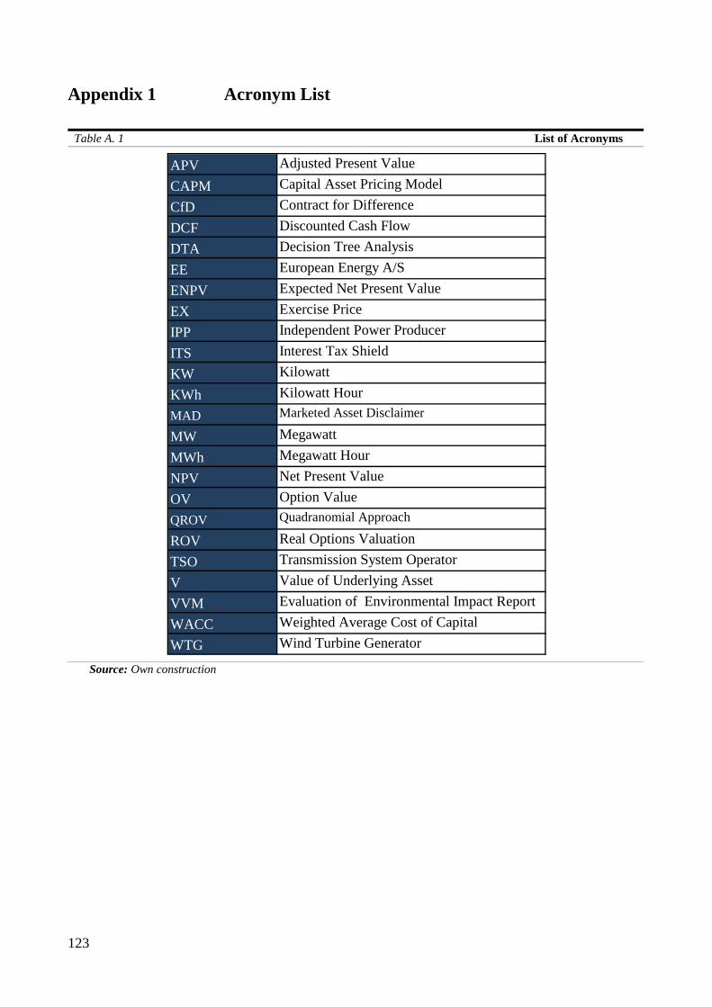
123

Appendix 1 Acronym List

Table A. 1 List of Acronyms


APV Adjusted Present ValueCAPM Capital Asset Pricing ModelCfD Contract for DifferenceDCF Discounted Cash FlowDTA Decision Tree AnalysisEE European Energy A/SENPV Expected Net Present ValueEX Exercise PriceIPP Independent Power ProducerITS Interest Tax ShieldKW KilowattKWh Kilowatt HourMAD Marketed Asset Disclaimer

MW MegawattMWh Megawatt HourNPV Net Present ValueOV Option ValueQROV Quadranomial Approach

ROV Real Options ValuationTSO Transmission System OperatorV Value of Underlying AssetVVM Evaluation of Environmental Impact ReportWACC Weighted Average Cost of CapitalWTG Wind Turbine Generator

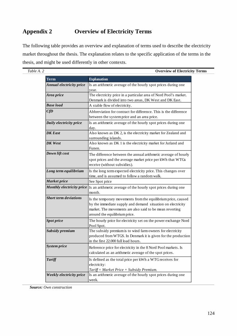
124

Appendix 2 Overview of Electricity Terms

The following table provides an overview and explanation of terms used to describe the electricity

market throughout the thesis. The explanation relates to the specific application of the terms in the

thesis, and might be used differently in other contexts.

Table A. 2 Overview of Electricity Terms


Term ExplanationAnnual electricity price Is an arithmetic average of the hourly spot prices during one

year.Area price The electricity price in a particular area of Nord Pool’s market.

Denmark is divided into two areas, DK West and DK East.Base load A stable flow of electricity.CfD Abbreviation for contract for difference. This is the difference

between the system price and an area price.Daily electricity price Is an arithmetic average of the hourly spot prices during one

day.DK East Also known as DK 2, is the electricity market for Zealand and

surrounding islands. DK West Also known as DK 1 is the electricity market for Jutland and

Funen.Down lift cost The difference between the annual arithmetic average of hourly

spot prices and the average market price per kWh that WTGs receive (without subsidies).

Long term equilibrium Is the long term expected electricity price. This changes over time, and is assumed to follow a random walk.

Market price See Spot price Monthly electricity price Is an arithmetic average of the hourly spot prices during one

month.Short term deviations Is the temporary movements from the equilibrium price, caused

by the immediate supply and demand situation on electricity market. The movements are also said to be mean reverting around the equilibrium price.

Spot price The hourly price for electricity set on the power exchange Nord Pool Spot.

Subsidy premium The subsidy premium is to wind farm owners for electricity produced from WTGS. In Denmark it is given for the production in the first 22.000 full load hours.

System price Reference price for electricity in the 8 Nord Pool markets. Is calculated as an arithmetic average of the spot prices.

Tariff Is defined as the total price per kWh a WTG receives for electricity: Tariff = Market Price + Subsidy Premium.

Weekly electricity price Is an arithmetic average of the hourly spot prices during one week.

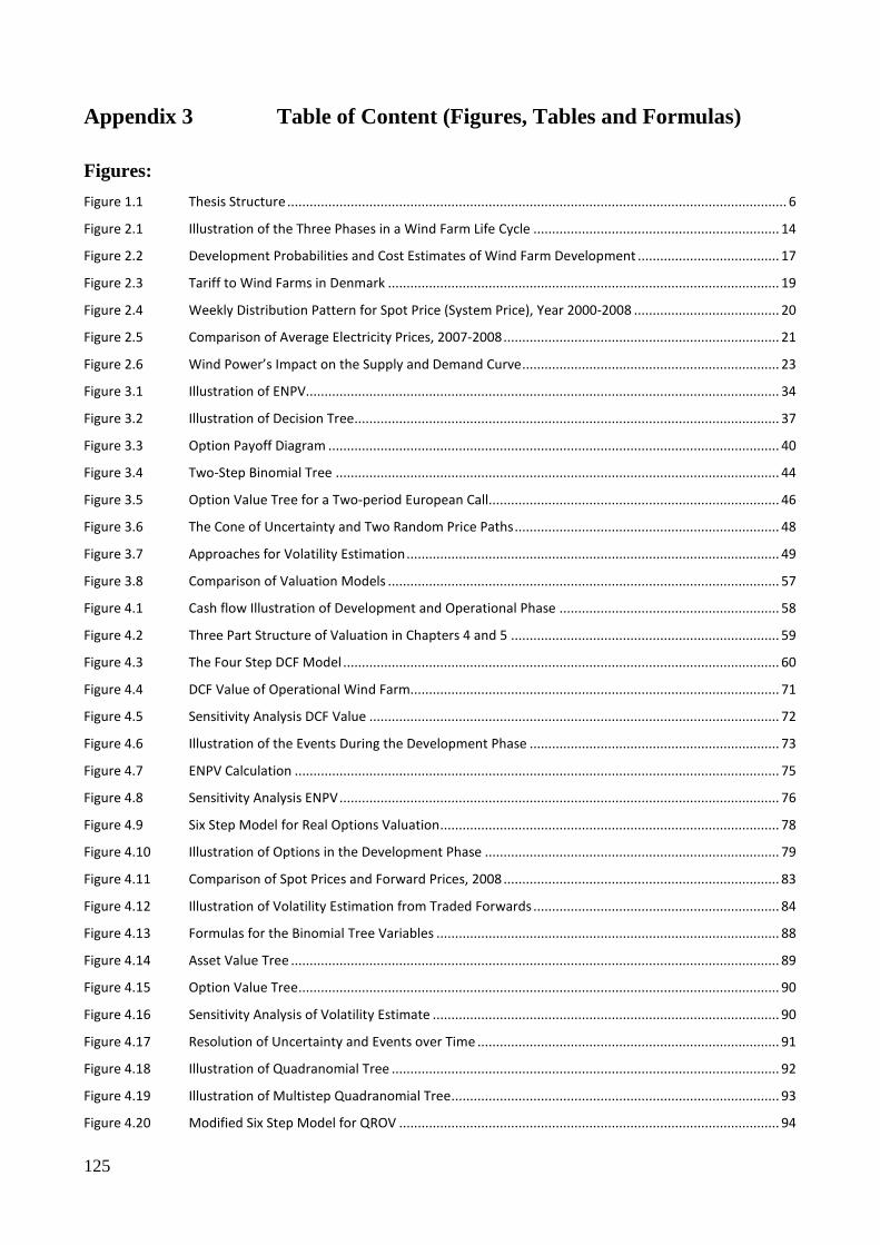
125

Appendix 3 Table of Content (Figures, Tables and Formulas)

Figures: Figure 1.1 Thesis Structure ...................................................................................................................................... 6

Figure 2.1 Illustration of the Three Phases in a Wind Farm Life Cycle .................................................................. 14

Figure 2.2 Development Probabilities and Cost Estimates of Wind Farm Development ...................................... 17

Figure 2.3 Tariff to Wind Farms in Denmark ......................................................................................................... 19

Figure 2.4 Weekly Distribution Pattern for Spot Price (System Price), Year 2000-2008 ....................................... 20

Figure 2.5 Comparison of Average Electricity Prices, 2007-2008 .......................................................................... 21

Figure 2.6 Wind Power’s Impact on the Supply and Demand Curve ..................................................................... 23

Figure 3.1 Illustration of ENPV............................................................................................................................... 34

Figure 3.2 Illustration of Decision Tree.................................................................................................................. 37

Figure 3.3 Option Payoff Diagram ......................................................................................................................... 40

Figure 3.4 Two-Step Binomial Tree ....................................................................................................................... 44

Figure 3.5 Option Value Tree for a Two-period European Call.............................................................................. 46

Figure 3.6 The Cone of Uncertainty and Two Random Price Paths ....................................................................... 48

Figure 3.7 Approaches for Volatility Estimation .................................................................................................... 49

Figure 3.8 Comparison of Valuation Models ......................................................................................................... 57

Figure 4.1 Cash flow Illustration of Development and Operational Phase ........................................................... 58

Figure 4.2 Three Part Structure of Valuation in Chapters 4 and 5 ........................................................................ 59

Figure 4.3 The Four Step DCF Model ..................................................................................................................... 60

Figure 4.4 DCF Value of Operational Wind Farm................................................................................................... 71

Figure 4.5 Sensitivity Analysis DCF Value .............................................................................................................. 72

Figure 4.6 Illustration of the Events During the Development Phase ................................................................... 73

Figure 4.7 ENPV Calculation .................................................................................................................................. 75

Figure 4.8 Sensitivity Analysis ENPV ...................................................................................................................... 76

Figure 4.9 Six Step Model for Real Options Valuation ........................................................................................... 78

Figure 4.10 Illustration of Options in the Development Phase ............................................................................... 79

Figure 4.11 Comparison of Spot Prices and Forward Prices, 2008 .......................................................................... 83

Figure 4.12 Illustration of Volatility Estimation from Traded Forwards .................................................................. 84

Figure 4.13 Formulas for the Binomial Tree Variables ............................................................................................ 88

Figure 4.14 Asset Value Tree ................................................................................................................................... 89

Figure 4.15 Option Value Tree ................................................................................................................................. 90

Figure 4.16 Sensitivity Analysis of Volatility Estimate ............................................................................................. 90

Figure 4.17 Resolution of Uncertainty and Events over Time ................................................................................. 91

Figure 4.18 Illustration of Quadranomial Tree ........................................................................................................ 92

Figure 4.19 Illustration of Multistep Quadranomial Tree ........................................................................................ 93

Figure 4.20 Modified Six Step Model for QROV ...................................................................................................... 94

126

Figure 4.21 Option Value Tree ................................................................................................................................. 95

Figure 4.22 Sensitivity Analysis QROV ..................................................................................................................... 96

Figure 4.23 Valuation of a Wind Farm Under Development ................................................................................... 97

Figure 5.1 ITS Value in the Operational Phase .................................................................................................... 105

Figure 5.2 ENPV Calculation Including Debt ........................................................................................................ 106

Figure 5.3 Change in ITS Value from different Electricity Price ........................................................................... 107

Figure 5.4 ITS Change from Leverage and Debt Risk Premium ........................................................................... 107

Figure 5.5 ITS Change from Leverage and Debt Risk Premium ........................................................................... 108

Figure 5.6 Modified Six Step Model including ITS ............................................................................................... 109

Figure 5.7 Asset Value Tree (Including ITS) ......................................................................................................... 110

Figure 5.8 Option Value Tree (Including ITS) ....................................................................................................... 110

Figure 6.1 Six Step Model for ROV of a Wind Farm Under Development ........................................................... 112

Formulas: Formula 3.1 Standard DCF Model ............................................................................................................................. 29

Formula 3.2 Capital Asset Pricing Model .................................................................................................................. 31

Formula 3.3 Intrinsic Option Value ........................................................................................................................... 40

Formula 3.4 Risk-neutral Probability Formula .......................................................................................................... 45

Formula 3.5 Option Value in Binomial Tree .............................................................................................................. 46

Formula 4.1 Expected Net Production ...................................................................................................................... 62

Formula 4.2 Down Lift Cost ...................................................................................................................................... 63

Formula 4.3 Calculation of Cost of Equity ................................................................................................................. 70

Formula 4.4 Calculation of Mid-year Factor ............................................................................................................. 71

Formula 4.5 Present Value of Underlying Asset ....................................................................................................... 80

Formula 4.6 Volatility of Logarithmic Change........................................................................................................... 85

Formula 4.7 Annual Volatility Using Square Root of Time Rule ................................................................................ 85

Formula 4.8 Option Value Quadranomial Approach ................................................................................................ 92

Formula 4.9 Option Value in the Quadranomial Approach (f=0) .............................................................................. 93

Formula 5.1 Weighted Average Cost of Capital ........................................................................................................ 99

Formula 5.2 Adjusted Present Value ...................................................................................................................... 100

Formula 5.3 Cost of Debt ........................................................................................................................................ 102

Formula 5.4 Cost of Debt (Calculation) ................................................................................................................... 103

Formula 5.5 Value of Interest Tax Shield ............................................................................................................... 104

Formula 5.6 Value of ITS in year 2.5 ....................................................................................................................... 109

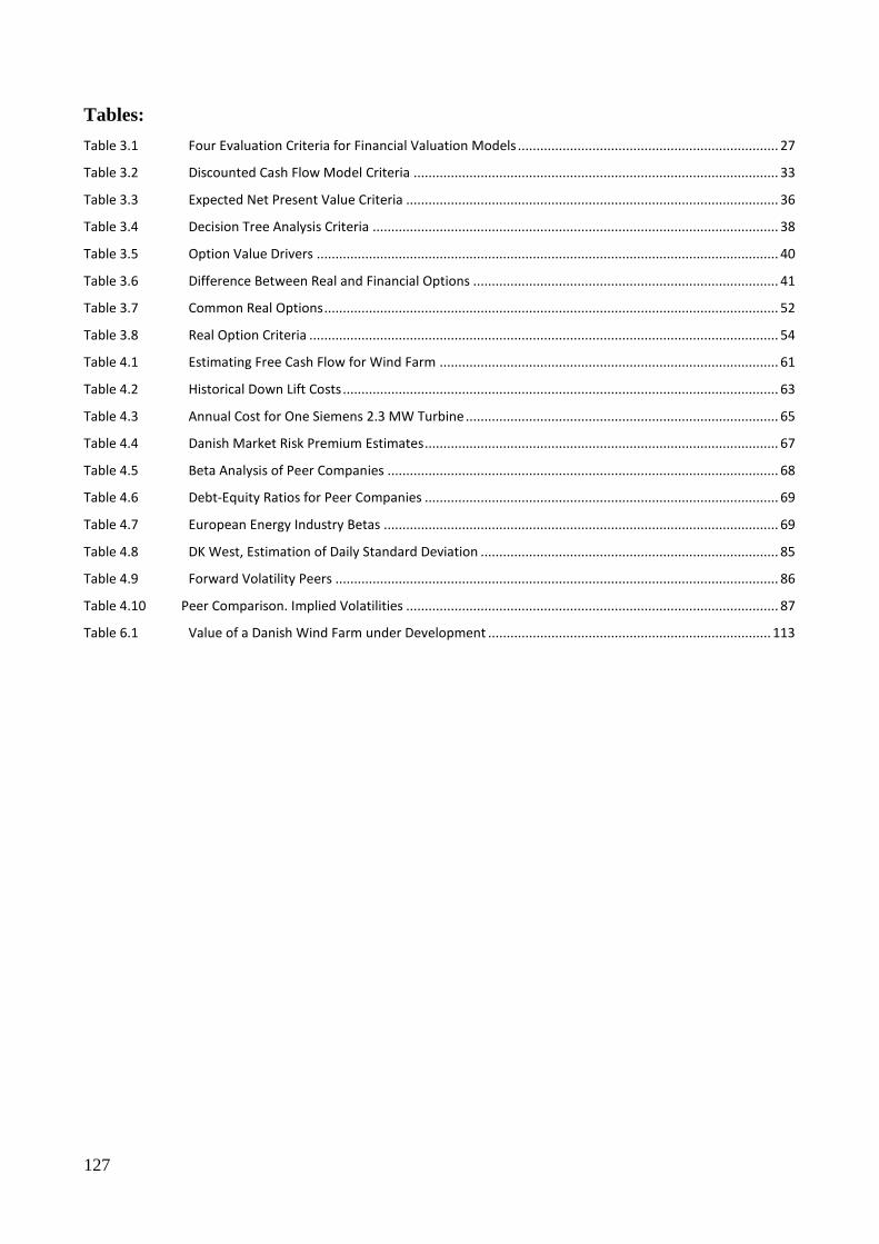
127

Tables: Table 3.1 Four Evaluation Criteria for Financial Valuation Models ...................................................................... 27

Table 3.2 Discounted Cash Flow Model Criteria .................................................................................................. 33

Table 3.3 Expected Net Present Value Criteria .................................................................................................... 36

Table 3.4 Decision Tree Analysis Criteria ............................................................................................................. 38

Table 3.5 Option Value Drivers ............................................................................................................................ 40

Table 3.6 Difference Between Real and Financial Options .................................................................................. 41

Table 3.7 Common Real Options .......................................................................................................................... 52

Table 3.8 Real Option Criteria .............................................................................................................................. 54

Table 4.1 Estimating Free Cash Flow for Wind Farm ........................................................................................... 61

Table 4.2 Historical Down Lift Costs ..................................................................................................................... 63

Table 4.3 Annual Cost for One Siemens 2.3 MW Turbine .................................................................................... 65

Table 4.4 Danish Market Risk Premium Estimates ............................................................................................... 67

Table 4.5 Beta Analysis of Peer Companies ......................................................................................................... 68

Table 4.6 Debt-Equity Ratios for Peer Companies ............................................................................................... 69

Table 4.7 European Energy Industry Betas .......................................................................................................... 69

Table 4.8 DK West, Estimation of Daily Standard Deviation ................................................................................ 85

Table 4.9 Forward Volatility Peers ....................................................................................................................... 86

Table 4.10 Peer Comparison. Implied Volatilities .................................................................................................... 87

Table 6.1 Value of a Danish Wind Farm under Development ............................................................................ 113

128

Appendix 4 Interviews with Danish Wind Farm Developers

To determine the stages of the development phase of wind farms in Denmark, we have interviewed

project manager Andreas Von Rosen and Head of Projects Jens-Peter Zink from our case company

European Energy, as well as project managers from two of the most experienced wind farms

developers in Denmark – DONG Energy and Vattenfall. A summary of the different interviews can

be seen in the table below. Before the interviews, we conducted a small amount of research to get

an initial idea of the development phase and the different stages. We therefore used the interviews

both to further define and understand the key hurdles and tasks within each stage, and to get

estimates of the costs and probabilities of success. A detailed description of the stages is given in

section 2.3 in the thesis. In all of the interviews we asked for estimates for average wind farms in

Denmark. We do however acknowledge that due to recent legislative changes and projects being

individual that neither our cost nor probabilities are exact. It is based on this acknowledgement that

we test the probabilities in the sensitivity analysis. The idea is that individual developers can refine

and collect better estimates for specific projects. The scope of this thesis is rather to develop a

general model, which can later be refined by better estimates. It should be noted that the

construction cost is specific to the wind farm, in our case 3 Siemens 2.3 MW 93m, and therefore

this cost has not been provided by other developers than European Energy.

Table A. 3 Interview with Andreas von Rosen, European Energy

Stage 1 2 3 4

Description Feasibility Studies and

Preapproval

VVM and

Final Approval

Complaints and

Compensation Construction

Duration

(months) Approx. 6 9 to 12 Approx. 6 3 to 6

Costs (DKK) 75,000 500,000 300,000-600,000 61,000,000

Success

Probability 75% 90% 50-75% 100%

Comments

Is hard to make a clear

distinction between this and pre-

development phase

Important stage,

much value is

created here

The duration and cost

of this stage is very site

dependent

-


129

Table A. 4 Interview with Jens-Peter Zink, European Energy

Stage 1 2 3 4

Description Feasibility Studies

and Preapproval

VVM and Final

Approval

Complaints and


Duration

(months) 6 6 to 12 Unsure 6

Costs (DKK) 100,000 300,000 to 500,000 Unsure N/A

Success

Probability 50% 85% Unsure 100%

Comments N/A A stage with a tendency

of “unpleasant surprises”

Did not want to

comment on this.

In theory it should done in

three months but something

always end taking longer than

expected


Table A. 5 Interview with Henriette Holm Mørch and Birte Hansen, DONG Energy

Stage 1 2 3 4


and Preapproval

VVM and Final

Approval

Complaints and


Duration

(months) 3 to 6 6 to 12 6 6-12

Costs (DKK) Unsure 500,000 to 750,000 500,000

Success

Probability 50% 50% 70% 100%

Comments Very variable and

independent stage. N/A

Cost represents

measurement of noise and

shadow effects due to

complaints but do not

account for compensation.

Many people tend to

underestimate this stage. It is

important that it is done

properly, which takes time.


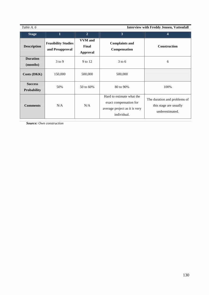
130

Table A. 6 Interview with Freddy Jensen, Vattenfall

Stage 1 2 3 4


and Preapproval

VVM and

Final

Approval

Complaints and


Duration

(months) 3 to 9 9 to 12 3 to 6 6

Costs (DKK) 150,000 500,000 500,000

Success

Probability 50% 50 to 60% 80 to 90% 100%

Comments N/A N/A

Hard to estimate what the

exact compensation for

average project as it is very

individual.

The duration and problems of

this stage are usually

underestimated.


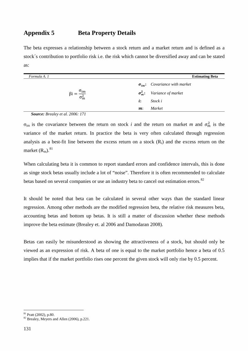
131

Appendix 5 Beta Property Details

The beta expresses a relationship between a stock return and a market return and is defined as a

stock´s contribution to portfolio risk i.e. the risk which cannot be diversified away and can be stated

as:

Formula A. 1 Estimating Beta

βi =σimσm2

𝝈𝒊𝒎: Covariance with market

𝝈𝒎𝟐 : Variance of market

𝒊: Stock i

𝒎: Market


σim is the covariance between the return on stock i and the return on market m and 𝜎𝑚2 is the

variance of the market return. In practice the beta is very often calculated through regression

analysis as a best-fit line between the excess return on a stock (Ri) and the excess return on the

market (Rm).81

When calculating beta it is common to report standard errors and confidence intervals, this is done

as singe stock betas usually include a lot of “noise”. Therefore it is often recommended to calculate

betas based on several companies or use an industry beta to cancel out estimation errors.82

It should be noted that beta can be calculated in several other ways than the standard linear

regression. Among other methods are the modified regression beta, the relative risk measures beta,

accounting betas and bottom up betas. It is still a matter of discussion whether these methods

improve the beta estimate (Brealey et. al 2006 and Damodaran 2008).

Betas can easily be misunderstood as showing the attractiveness of a stock, but should only be

viewed as an expression of risk. A beta of one is equal to the market portfolio hence a beta of 0.5

implies that if the market portfolio rises one percent the given stock will only rise by 0.5 percent.

81 Pratt (2002), p.80. 82 Brealey, Meyers and Allen (2006), p.221.

132

Appendix 6 CAPM Assumptions

Table A. 7 The CAPM Assumptions 1. No transaction costs.

2. Any asset is infinitely divisible.

3. No personal income tax.

4. Individual actions cannot influence stock price.

5. All investment decisions are based on expected

return and standard deviation of portfolio.

6. Unlimited short sales allowed.

7. Unlimited lending and borrowing at risk free rate.

8. Investors are concerned with mean and variance of

returns.

9. All investors are assumed to have identical

expectations, with respect to the necessary inputs to

the portfolio decision.

10. All assets are marketable.

Source: Elton et al. 2007: 285

As can be seen from the above table the assumptions of the CAPM are clearly not realistic.

However the actual test of a model should not be its assumptions but instead how well its results

compares to actual observations (Elton et al. 2007: 285). As argued for in Chapter three despite the

assumption of the CAPM being very strong it actually performs remarkably well when applied to

stock returns.

133

Appendix 7 Overview of ENPV Methods

Table A. 8 ENPV Assumptions Review

Author(s) Discount Rate Failure Probabilities Comments

Kellogg and Charnes

(2000)

A different rate for

development and market

phase.

Based on both market and

development failure. N/A

Koller, Goedhart and

Wessels (2005)

Risk free for development

phase and opportunity

cost of capital for market

phase.

Based on development

failure. N/A

Pandey (2003) Risk free for both phases. Not clear uses illustrative

rates.

Admits that market state

might not be risk free but

uses for illustration.

Shockley (2007)

Risk free for development

and WACC for market

phase.

Development failure.

Acknowledges that risk

free rate does not capture

market uncertainty.

Villiger and Bogdan

(2005)

Risk free plus a risk

premium for both phases.

Includes both market and

development failure.

Discuss the problem of

accounting for economic

failure in probabilities.

Willigers and Hansen

(2008)

Risk free plus a risk

premium for both phases.

Includes both market and

development failure.

Acknowledge double

risking.


From the above it can be seen that not all the authors agree with regard to which discount rate to use

in the ENPV. We have however chosen to follow the arguments presented in Koller et al. (2005)

and Shockley (2007). This is based on the notion that the other authors, who apply different rates

acknowledge the inconsistency of their method e.g. Villiger and Bogdan (2005) and Willigers and

Hansen (2008). Kellogg and Charnes (2000) combine market uncertainty and probabilities of failure

events in their discount rate, which leads to confusion. Pandey (2003) is only interested in

illustrating the approach and states that his discount rates are merely illustrative.

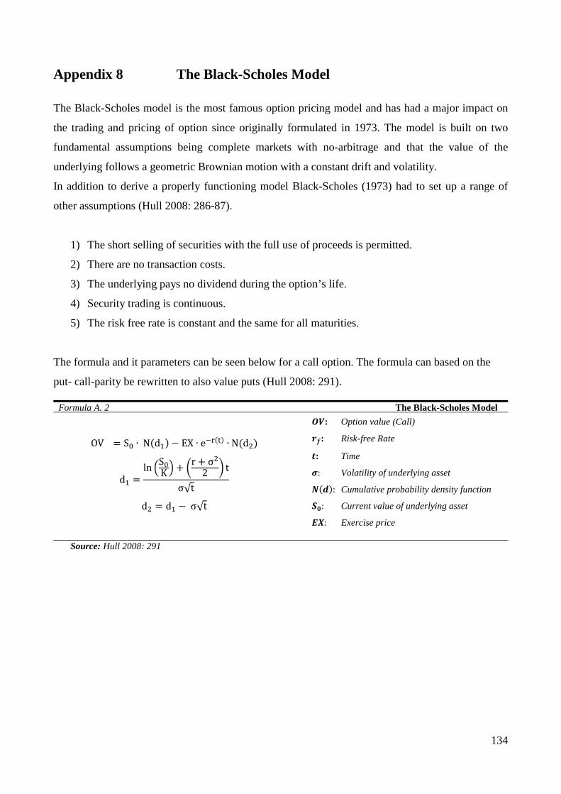
134

Appendix 8 The Black-Scholes Model

The Black-Scholes model is the most famous option pricing model and has had a major impact on

the trading and pricing of option since originally formulated in 1973. The model is built on two

fundamental assumptions being complete markets with no-arbitrage and that the value of the

underlying follows a geometric Brownian motion with a constant drift and volatility.

In addition to derive a properly functioning model Black-Scholes (1973) had to set up a range of

other assumptions (Hull 2008: 286-87).

1) The short selling of securities with the full use of proceeds is permitted.

2) There are no transaction costs.

3) The underlying pays no dividend during the option’s life.

4) Security trading is continuous.

5) The risk free rate is constant and the same for all maturities.

The formula and it parameters can be seen below for a call option. The formula can based on the

put- call-parity be rewritten to also value puts (Hull 2008: 291).

Formula A. 2 The Black-Scholes Model

OV = S0 ∙ N(d1)− EX ∙ e−r(t) ∙ N(d2)

d1 =ln �S0

K � + �r + σ22 � t

σ√t

d2 = d1 − σ√t

𝑶𝑽: Option value (Call)

𝒓𝒇: Risk-free Rate

𝒕: Time

𝝈: Volatility of underlying asset

𝑵(𝒅): Cumulative probability density function

𝑺𝟎: Current value of underlying asset


Source: Hull 2008: 291

135

Appendix 9 Cost Estimates for Operational Wind Farm

The cost estimates for the operational phase are estimated from 3 different sources: Danish Wind

Turbine Owners’ Association (dkvind), European Energy and Vognkær Ny Møllelaug. The two

prior sources have estimated the costs of a Siemens 2.3 MW WTG with rotor diameter of 93 m,

whereas the last one is for a Vestas 3.0 MW. These are different turbines, but their operational costs

are usually relatively similar.

The first cost estimation is from Jørn Larsen, an economic advisor specialized in the economics and

tax issues of WTGs from Danish Wind Turbine Owners’ Association. The estimates are for a

Siemens 2.3 MW 93 m WTG.

Cost Estimation 1, Siemens 2.3 MW Interview with Jørn Larsen, dkvind

Source: E-mail correspondence with Jørn Larsen, dkvind, 16th November 2009.

The second cost estimation is from the Andreas Von Rosen, Project Manager for European

Energy’s assets in Denmark and England, and is also made for a Siemens 2.3 MW, 93 m WTG.

Cost Estimation 2, Siemens 2.3 MW Interview with Andreas Von Rosen, European Energy

Source: Prospect from Vognkær Ny Møllelaug.

The last estimation is a wind farm prospect from Vognkær Ny Møllelaug for two Vestas 3.0 MW

turbines. Even though this is a different and larger turbine than the ones presented in our case wind

Expense: Estimations of Annual Costs/WTGService from Year 3 The 2010 price for such an agreement is: DKK

203,400/YearTechnical Management The price for such an agreement can vary, but is

approxemately 5-8 øre/kWh, depending on the location of the WTG.

Insurance: The 2010 price is approximately DKK 150,000/Year

Land Lease: 3-4 % of the revenueAdministration: DKK 50,000 - 100,000/YearOwn energy consumption: UnknownGrid Loss: Approximately 2%

Expense: Estimations of Annual Costs/WTGService from Year 3 DKK 200,000/YearTechnical Management 5 øre/kWhInsurance: DKK 150,000/YearLand Lease: 2-3% of revenueAdministration: DKK 100,000/YearOwn energy consumption: DKK 30,000/Year

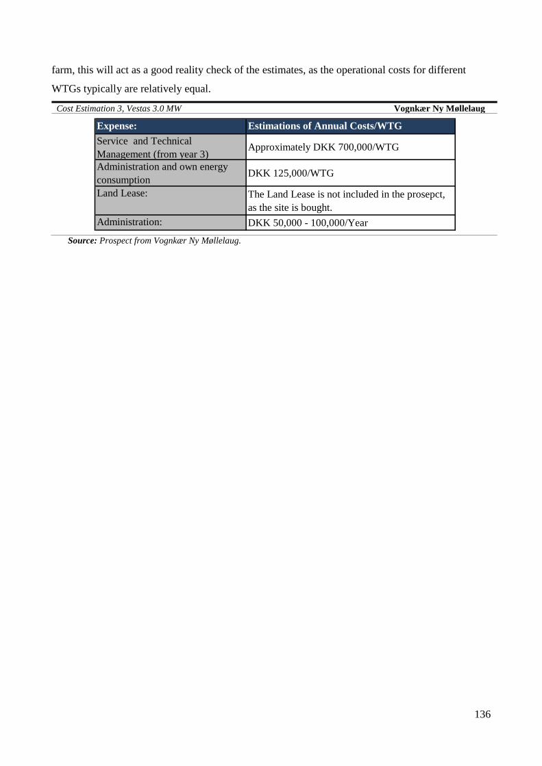
136

farm, this will act as a good reality check of the estimates, as the operational costs for different

WTGs typically are relatively equal.

Cost Estimation 3, Vestas 3.0 MW Vognkær Ny Møllelaug

Source: Prospect from Vognkær Ny Møllelaug.

Expense: Estimations of Annual Costs/WTGService and Technical Management (from year 3)

Approximately DKK 700,000/WTG

Administration and own energy consumption DKK 125,000/WTG

Land Lease: The Land Lease is not included in the prosepct, as the site is bought.

Administration: DKK 50,000 - 100,000/Year

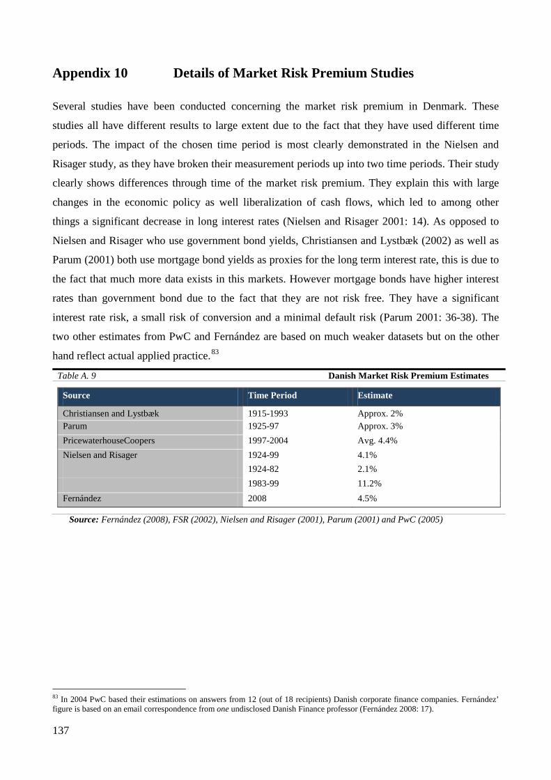
137

Appendix 10 Details of Market Risk Premium Studies

Several studies have been conducted concerning the market risk premium in Denmark. These

studies all have different results to large extent due to the fact that they have used different time

periods. The impact of the chosen time period is most clearly demonstrated in the Nielsen and

Risager study, as they have broken their measurement periods up into two time periods. Their study

clearly shows differences through time of the market risk premium. They explain this with large

changes in the economic policy as well liberalization of cash flows, which led to among other

things a significant decrease in long interest rates (Nielsen and Risager 2001: 14). As opposed to

Nielsen and Risager who use government bond yields, Christiansen and Lystbæk (2002) as well as

Parum (2001) both use mortgage bond yields as proxies for the long term interest rate, this is due to

the fact that much more data exists in this markets. However mortgage bonds have higher interest

rates than government bond due to the fact that they are not risk free. They have a significant

interest rate risk, a small risk of conversion and a minimal default risk (Parum 2001: 36-38). The

two other estimates from PwC and Fernández are based on much weaker datasets but on the other

hand reflect actual applied practice.83

Table A. 9 Danish Market Risk Premium Estimates

Source Time Period Estimate

Christiansen and Lystbæk 1915-1993 Approx. 2% Parum 1925-97 Approx. 3% PricewaterhouseCoopers 1997-2004 Avg. 4.4% Nielsen and Risager 1924-99 4.1% 1924-82 2.1% 1983-99 11.2% Fernández 2008 4.5%

Source: Fernández (2008), FSR (2002), Nielsen and Risager (2001), Parum (2001) and PwC (2005)

83 In 2004 PwC based their estimations on answers from 12 (out of 18 recipients) Danish corporate finance companies. Fernández’ figure is based on an email correspondence from one undisclosed Danish Finance professor (Fernández 2008: 17).

138

Appendix 11 Beta Estimation Peers84

Alerion Clean Power SpA Symbol ARN:IM Country of Origin Italy Power Technologies Wind, Solar, Biomass Geographical Presence Italy, Netherlands, Belgium, Romania, Bulgaria, Albania and Turkey85 Installed Capacity (MW) 230 MW

Alerion Cleanpower SpA is an Italian renewable energy independent power producer. The

Company's activities include wind, solar, and biomass projects. It currently only has operational

projects in Italy but is looking at several new markets both in Eastern and Western Europe.

Greentech Energy Systems A/S Symbol GES:DC Country of Origin Denmark Power Technologies Wind Geographical Presence Denmark, Germany, Poland, Italy and Norway. Installed Capacity (MW) 75

Greentech Energy Systems A/S owns wind turbines and invests in and helps develop companies

that produce wind generated electricity. The Company owns several wind turbines in Denmark and

takes part in international wind power projects. Greentech primarily invests in EURO-related

countries with attractive wind conditions and higher electricity prices.

Theolia SA Symbol TEO:FP Country of Origin France Power Technologies Wind Geographical Presence France, Germany, Morocco, Italy, Brazil and India. Installed Capacity (MW) 421

Theolia is a French IPP operating within the wind energy sector. Theolia is involved in the

development, construction, ownership and management (for third parties) of wind farms. It is

already present in Morocco but wishes to expand more to emerging markets, while at the same time

also growing in Western Europe.

84 Data from company homepages. 85 Italics mean company is only present with projects under development.

139

Iberdrola Renovables SA Symbol IBR: SM

Country of Origin Spain

Power Technologies Wind, Biomass, Hydro and Solar

Geographical Presence Europe, South and North America

Installed Capacity (MW) ~10,700 MW

Iberdrola Renovables is the world larges renewable asset owner and partly owned by Iberdrola SA,

the fourth largest utility in the world. The company is involved in the development, construction

and ownership of these assets. The company’s three main markets are Spain, UK and USA but they

have a significant presence in other countries as well.

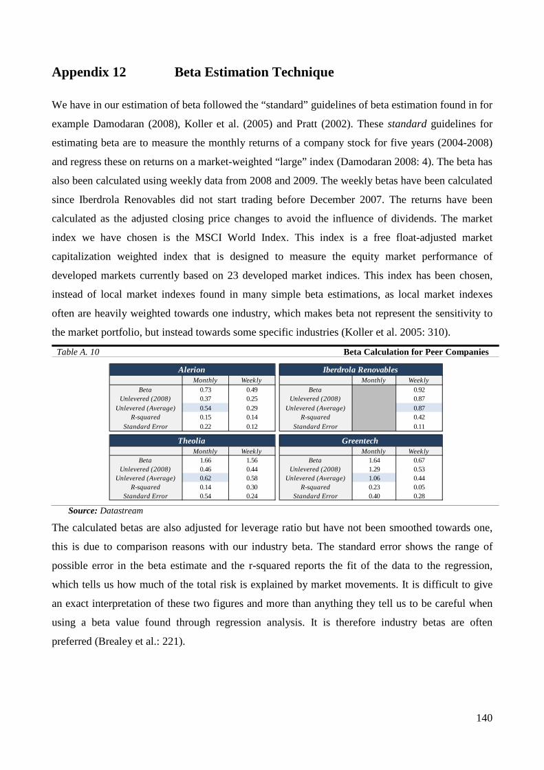
140

Appendix 12 Beta Estimation Technique

We have in our estimation of beta followed the “standard” guidelines of beta estimation found in for

example Damodaran (2008), Koller et al. (2005) and Pratt (2002). These standard guidelines for

estimating beta are to measure the monthly returns of a company stock for five years (2004-2008)

and regress these on returns on a market-weighted “large” index (Damodaran 2008: 4). The beta has

also been calculated using weekly data from 2008 and 2009. The weekly betas have been calculated

since Iberdrola Renovables did not start trading before December 2007. The returns have been

calculated as the adjusted closing price changes to avoid the influence of dividends. The market

index we have chosen is the MSCI World Index. This index is a free float-adjusted market

capitalization weighted index that is designed to measure the equity market performance of

developed markets currently based on 23 developed market indices. This index has been chosen,

instead of local market indexes found in many simple beta estimations, as local market indexes

often are heavily weighted towards one industry, which makes beta not represent the sensitivity to

the market portfolio, but instead towards some specific industries (Koller et al. 2005: 310).

Table A. 10 Beta Calculation for Peer Companies

Source: Datastream

The calculated betas are also adjusted for leverage ratio but have not been smoothed towards one,

this is due to comparison reasons with our industry beta. The standard error shows the range of

possible error in the beta estimate and the r-squared reports the fit of the data to the regression,

which tells us how much of the total risk is explained by market movements. It is difficult to give

an exact interpretation of these two figures and more than anything they tell us to be careful when

using a beta value found through regression analysis. It is therefore industry betas are often

preferred (Brealey et al.: 221).

Monthly Weekly Monthly WeeklyBeta 0.73 0.49 Beta 0.92

Unlevered (2008) 0.37 0.25 Unlevered (2008) 0.87Unlevered (Average) 0.54 0.29 Unlevered (Average) 0.87

R-squared 0.15 0.14 R-squared 0.42Standard Error 0.22 0.12 Standard Error 0.11

Monthly Weekly Monthly WeeklyBeta 1.66 1.56 Beta 1.64 0.67

Unlevered (2008) 0.46 0.44 Unlevered (2008) 1.29 0.53Unlevered (Average) 0.62 0.58 Unlevered (Average) 1.06 0.44

R-squared 0.14 0.30 R-squared 0.23 0.05Standard Error 0.54 0.24 Standard Error 0.40 0.28

Alerion Iberdrola Renovables

Theolia Greentech

141

Appendix 13 Volatility Estimation from Forward Prices

Forward data year 2007, for the DK West forward expiring in year 2010:

...Continued ...Continued

DateSystem Price CfD

Forward DK West

Log change Date

System Price CfD

Forward DK West Log change Date

System Price CfD

Forward DK West Log change

02-01-07 42.4 4.58 46.98 07-05-07 44.24 5.5 49.74 0.02% 05-09-07 46.65 4.53 51.18 -0.29%03-01-07 42.2 4.5 46.7 -0.60% 08-05-07 44.05 5.5 49.55 -0.38% 06-09-07 46.6 4.55 51.15 -0.06%04-01-07 42 4.68 46.68 -0.04% 09-05-07 44.3 5.5 49.8 0.50% 07-09-07 46.55 4.53 51.08 -0.14%05-01-07 41.38 4.63 46.01 -1.45% 10-05-07 44.25 5.5 49.75 -0.10% 10-09-07 46.27 4.68 50.95 -0.25%08-01-07 40 4.63 44.63 -3.05% 11-05-07 44.48 5.5 49.98 0.46% 11-09-07 46.4 4.55 50.95 0.00%09-01-07 40.29 4.63 44.92 0.65% 14-05-07 44.44 5.5 49.94 -0.08% 12-09-07 46.63 4.53 51.16 0.41%10-01-07 40.6 4.65 45.25 0.73% 15-05-07 44.6 5.63 50.23 0.58% 13-09-07 46.35 4.55 50.9 -0.51%11-01-07 41.45 4.98 46.43 2.57% 16-05-07 44.75 5.48 50.23 0.00% 14-09-07 46.5 4.63 51.13 0.45%12-01-07 42.4 4.9 47.3 1.86% 18-05-07 45.1 5.5 50.6 0.73% 17-09-07 46.55 4.53 51.08 -0.10%15-01-07 42.6 4.9 47.5 0.42% 21-05-07 45.25 5.5 50.75 0.30% 18-09-07 46.55 4.55 51.1 0.04%16-01-07 42.75 4.9 47.65 0.32% 22-05-07 45.28 5.5 50.78 0.06% 19-09-07 46.6 4.55 51.15 0.10%17-01-07 42.65 5.5 48.15 1.04% 23-05-07 45.28 5.5 50.78 0.00% 20-09-07 46.9 4.55 51.45 0.58%18-01-07 42.45 5.5 47.95 -0.42% 24-05-07 45.45 5.5 50.95 0.33% 21-09-07 47.37 4.58 51.95 0.97%19-01-07 42.35 5.5 47.85 -0.21% 25-05-07 45.63 5.5 51.13 0.35% 24-09-07 47.13 4.53 51.66 -0.56%22-01-07 42.25 5.55 47.8 -0.10% 29-05-07 46.15 5.5 51.65 1.01% 25-09-07 46.95 4.53 51.48 -0.35%23-01-07 41.95 5.5 47.45 -0.73% 30-05-07 45.85 5.5 51.35 -0.58% 26-09-07 47.25 4.53 51.78 0.58%24-01-07 42.2 5.63 47.83 0.80% 31-05-07 45.7 5.5 51.2 -0.29% 27-09-07 47.3 4.53 51.83 0.10%25-01-07 42.08 5.5 47.58 -0.52% 01-06-07 45.68 5.25 50.93 -0.53% 28-09-07 47.5 4.28 51.78 -0.10%26-01-07 42.2 5.5 47.7 0.25% 04-06-07 46.75 5.13 51.88 1.85% 01-10-07 47.63 4.5 52.13 0.67%29-01-07 41.95 5.58 47.53 -0.36% 05-06-07 46.75 5.25 52 0.23% 02-10-07 47.65 4.53 52.18 0.10%30-01-07 42.2 5.55 47.75 0.46% 06-06-07 46.9 4.75 51.65 -0.68% 03-10-07 47.4 4.53 51.93 -0.48%31-01-07 42.15 5.6 47.75 0.00% 07-06-07 46.3 4.75 51.05 -1.17% 04-10-07 47.5 4.58 52.08 0.29%01-02-07 42 5.55 47.55 -0.42% 08-06-07 46.58 4.75 51.33 0.55% 05-10-07 47.7 4.5 52.2 0.23%02-02-07 41.7 5.5 47.2 -0.74% 11-06-07 46.95 4.75 51.7 0.72% 08-10-07 47.7 4.65 52.35 0.29%05-02-07 41.83 5.5 47.33 0.28% 12-06-07 46.95 4.75 51.7 0.00% 09-10-07 47.8 4.63 52.43 0.15%06-02-07 42.2 5.53 47.73 0.84% 13-06-07 47.1 4.75 51.85 0.29% 10-10-07 48.6 4.63 53.23 1.51%07-02-07 41.9 5.53 47.43 -0.63% 14-06-07 47.63 4.25 51.88 0.06% 11-10-07 48.65 4.68 53.33 0.19%08-02-07 41.9 5.5 47.4 -0.06% 15-06-07 47.28 4.5 51.78 -0.19% 12-10-07 49.53 4.63 54.16 1.54%09-02-07 41.9 5.5 47.4 0.00% 18-06-07 46.85 4.5 51.35 -0.83% 15-10-07 49.65 4.63 54.28 0.22%12-02-07 41.92 5.5 47.42 0.04% 19-06-07 46.25 4.5 50.75 -1.18% 16-10-07 49.9 4.4 54.3 0.04%13-02-07 41.69 5.5 47.19 -0.49% 20-06-07 46.8 4.5 51.3 1.08% 17-10-07 50.03 4.63 54.66 0.66%14-02-07 41.55 5.53 47.08 -0.23% 21-06-07 47.25 4.5 51.75 0.87% 18-10-07 50.28 4.63 54.91 0.46%15-02-07 41.49 5.5 46.99 -0.19% 22-06-07 47.2 4.5 51.7 -0.10% 19-10-07 50.85 4.63 55.48 1.03%16-02-07 41.4 5.5 46.9 -0.19% 25-06-07 47.1 4.5 51.6 -0.19% 22-10-07 50.25 4.63 54.88 -1.09%19-02-07 41.03 5.45 46.48 -0.90% 26-06-07 47.3 4.5 51.8 0.39% 23-10-07 50.65 4.68 55.33 0.82%20-02-07 40.8 5.4 46.2 -0.60% 27-06-07 47.1 4.5 51.6 -0.39% 24-10-07 51.2 4.63 55.83 0.90%21-02-07 41.15 5.65 46.8 1.29% 28-06-07 47.15 4.5 51.65 0.10% 25-10-07 51.5 4.63 56.13 0.54%22-02-07 41.15 5.68 46.83 0.06% 29-06-07 47.2 4.5 51.7 0.10% 26-10-07 51.2 4.63 55.83 -0.54%23-02-07 41.5 5.58 47.08 0.53% 02-07-07 47.15 4.5 51.65 -0.10% 29-10-07 51.48 4.63 56.11 0.50%26-02-07 42.1 5.53 47.63 1.16% 03-07-07 46.7 4.5 51.2 -0.88% 30-10-07 50.28 4.63 54.91 -2.16%27-02-07 41.75 5.5 47.25 -0.80% 04-07-07 46.25 4.75 51 -0.39% 31-10-07 50.4 4.63 55.03 0.22%28-02-07 41.75 5.5 47.25 0.00% 05-07-07 46.5 4.75 51.25 0.49% 01-11-07 50 4.63 54.63 -0.73%01-03-07 42.08 5.5 47.58 0.70% 06-07-07 46.6 4.75 51.35 0.19% 02-11-07 50.23 4.63 54.86 0.42%02-03-07 41.7 5.5 47.2 -0.80% 09-07-07 46.4 4.75 51.15 -0.39% 05-11-07 49.3 4.63 53.93 -1.71%05-03-07 41.1 5.5 46.6 -1.28% 10-07-07 46.3 4.75 51.05 -0.20% 06-11-07 49.9 4.63 54.53 1.11%06-03-07 41.5 5.38 46.88 0.60% 11-07-07 46.2 4.75 50.95 -0.20% 07-11-07 50 4.63 54.63 0.18%07-03-07 41.5 5.38 46.88 0.00% 12-07-07 45.9 4.9 50.8 -0.29% 08-11-07 50.25 4.63 54.88 0.46%08-03-07 41.73 5.38 47.11 0.49% 13-07-07 45.95 4.88 50.83 0.06% 09-11-07 50.35 4.63 54.98 0.18%09-03-07 41.7 5.38 47.08 -0.06% 16-07-07 46.45 4.88 51.33 0.98% 12-11-07 49.8 4.63 54.43 -1.01%12-03-07 41.7 5.38 47.08 0.00% 17-07-07 46.5 4.83 51.33 0.00% 13-11-07 49.9 4.63 54.53 0.18%13-03-07 41.8 5.5 47.3 0.47% 18-07-07 46.28 4.78 51.06 -0.53% 14-11-07 49.75 4.63 54.38 -0.28%14-03-07 41.75 5.5 47.25 -0.11% 19-07-07 46.65 4.75 51.4 0.66% 15-11-07 49.75 4.7 54.45 0.13%15-03-07 41.86 5.5 47.36 0.23% 20-07-07 46.65 4.7 51.35 -0.10% 16-11-07 49.88 4.63 54.51 0.11%16-03-07 41.85 5.5 47.35 -0.02% 23-07-07 46.53 4.75 51.28 -0.14% 19-11-07 50.05 4.63 54.68 0.31%19-03-07 41.73 5.5 47.23 -0.25% 24-07-07 46.5 4.75 51.25 -0.06% 20-11-07 50.35 4.63 54.98 0.55%20-03-07 41.9 5.5 47.4 0.36% 25-07-07 46.8 4.63 51.43 0.35% 21-11-07 50.3 4.65 54.95 -0.05%21-03-07 42.2 5.5 47.7 0.63% 26-07-07 46.78 4.5 51.28 -0.29% 22-11-07 50.26 4.65 54.91 -0.07%22-03-07 42.28 5.5 47.78 0.17% 27-07-07 46.7 4.5 51.2 -0.16% 23-11-07 50.2 4.75 54.95 0.07%23-03-07 42.51 5.5 48.01 0.48% 30-07-07 46.85 4.5 51.35 0.29% 26-11-07 50.2 4.63 54.83 -0.22%26-03-07 43.05 5.5 48.55 1.12% 31-07-07 47.5 4.5 52 1.26% 27-11-07 49.85 4.75 54.6 -0.42%27-03-07 43.05 5.5 48.55 0.00% 01-08-07 47.03 4.5 51.53 -0.91% 28-11-07 50.1 4.63 54.73 0.24%28-03-07 43 5.5 48.5 -0.10% 02-08-07 47.18 4.5 51.68 0.29% 29-11-07 49.75 4.85 54.6 -0.24%29-03-07 43.35 5.5 48.85 0.72% 03-08-07 47.1 4.5 51.6 -0.15% 30-11-07 49.6 4.73 54.33 -0.50%30-03-07 43.63 5.5 49.13 0.57% 06-08-07 46.88 4.5 51.38 -0.43% 03-12-07 49.85 4.68 54.53 0.37%02-04-07 43.25 5.5 48.75 -0.78% 07-08-07 46.5 4.5 51 -0.74% 04-12-07 50.2 4.65 54.85 0.59%03-04-07 43.33 5.5 48.83 0.16% 08-08-07 46.55 4.5 51.05 0.10% 05-12-07 50.25 4.65 54.9 0.09%04-04-07 43.25 5.5 48.75 -0.16% 09-08-07 46.53 4.5 51.03 -0.04% 06-12-07 49.95 4.7 54.65 -0.46%10-04-07 43.23 5.5 48.73 -0.04% 10-08-07 46.48 4.5 50.98 -0.10% 07-12-07 50.16 5.2 55.36 1.29%11-04-07 43.5 5.53 49.03 0.61% 13-08-07 46.45 4.5 50.95 -0.06% 10-12-07 50.1 5.2 55.3 -0.11%12-04-07 43.68 5.63 49.31 0.57% 14-08-07 46.43 4.5 50.93 -0.04% 11-12-07 50.2 5.2 55.4 0.18%13-04-07 43.75 5.7 49.45 0.28% 15-08-07 46.25 4.5 50.75 -0.35% 12-12-07 50 5.25 55.25 -0.27%16-04-07 44.05 5.6 49.65 0.40% 16-08-07 45.93 4.5 50.43 -0.63% 13-12-07 50.3 5.33 55.63 0.69%17-04-07 44 5.6 49.6 -0.10% 17-08-07 45.85 4.5 50.35 -0.16% 14-12-07 50.1 5.38 55.48 -0.27%18-04-07 43.83 5.6 49.43 -0.34% 20-08-07 45.9 4.5 50.4 0.10% 17-12-07 50 5.35 55.35 -0.23%19-04-07 43.6 5.6 49.2 -0.47% 21-08-07 46.1 4.5 50.6 0.40% 18-12-07 50.15 5.43 55.58 0.41%20-04-07 43.7 5.55 49.25 0.10% 22-08-07 45.95 4.5 50.45 -0.30% 19-12-07 50.25 5.6 55.85 0.48%23-04-07 43.9 5.63 49.53 0.57% 23-08-07 46 4.63 50.63 0.36% 20-12-07 50.5 5.53 56.03 0.32%24-04-07 43.78 5.75 49.53 0.00% 24-08-07 45.7 4.25 49.95 -1.35% 21-12-07 50.5 5.53 56.03 0.00%25-04-07 44.1 5.5 49.6 0.14% 27-08-07 45.88 4.38 50.26 0.62% 27-12-07 50.78 5.53 56.31 0.50%26-04-07 43.88 5.63 49.51 -0.18% 28-08-07 45.97 4.13 50.1 -0.32% 28-12-07 50.88 5.23 56.11 -0.36%27-04-07 43.88 5.5 49.38 -0.26% 29-08-07 46.2 3.5 49.7 -0.80%30-04-07 44.14 5.5 49.64 0.53% 30-08-07 46.15 4.38 50.53 1.66%02-05-07 44 5.5 49.5 -0.28% 31-08-07 46.33 4.38 50.71 0.36% Annual Vol. 2007 10.09%03-05-07 44 5.5 49.5 0.00% 03-09-07 46.48 4.55 51.03 0.63%04-05-07 44.23 5.5 49.73 0.46% 04-09-07 46.8 4.53 51.33 0.59%

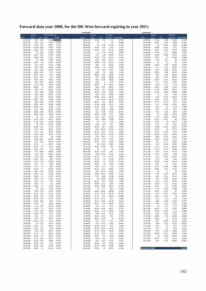
142




Forward DK West

Log change Date

System Price CfD


System Price CfD


02-01-08 50.3 5.58 55.88 06-05-08 53.85 7.15 61 -0.29% 03-09-08 60.2 9.98 70.18 0.33%03-01-08 50.6 5.75 56.35 0.84% 07-05-08 54 7 61 0.00% 04-09-08 60.45 9.63 70.08 -0.14%04-01-08 51.18 5.75 56.93 1.02% 08-05-08 54 7.08 61.08 0.13% 05-09-08 60 10.63 70.63 0.78%07-01-08 51.48 5.88 57.36 0.75% 09-05-08 54.65 7.15 61.8 1.17% 08-09-08 59.85 10.25 70.1 -0.75%08-01-08 52.05 5.83 57.88 0.90% 13-05-08 54.65 7.13 61.78 -0.03% 09-09-08 58.25 11.53 69.78 -0.46%09-01-08 52 5.83 57.83 -0.09% 14-05-08 55 7.15 62.15 0.60% 10-09-08 57.38 11.5 68.88 -1.30%10-01-08 52.05 5.93 57.98 0.26% 15-05-08 55.1 7.18 62.28 0.21% 11-09-08 57.65 11.38 69.03 0.22%11-01-08 51.85 5.68 57.53 -0.78% 16-05-08 55.55 7.18 62.73 0.72% 12-09-08 58.35 11 69.35 0.46%14-01-08 52 5.88 57.88 0.61% 19-05-08 56.5 7.03 63.53 1.27% 15-09-08 55.9 10.1 66 -4.95%15-01-08 51.95 5.9 57.85 -0.05% 20-05-08 56.98 7.13 64.11 0.91% 16-09-08 55 10 65 -1.53%16-01-08 51.3 5.95 57.25 -1.04% 21-05-08 58.4 7.13 65.53 2.19% 17-09-08 56.35 9.93 66.28 1.95%17-01-08 50.6 6.03 56.63 -1.09% 22-05-08 59.85 7.2 67.05 2.29% 18-09-08 57.1 9.25 66.35 0.11%18-01-08 50.1 6.18 56.28 -0.62% 23-05-08 60 7.85 67.85 1.19% 19-09-08 60.5 8.85 69.35 4.42%21-01-08 48.85 6.25 55.1 -2.12% 26-05-08 60.9 7.9 68.8 1.39% 22-09-08 60.25 9.08 69.33 -0.03%22-01-08 49.35 6.25 55.6 0.90% 27-05-08 60.95 7.93 68.88 0.12% 23-09-08 59.8 9.38 69.18 -0.22%23-01-08 49.15 6.25 55.4 -0.36% 28-05-08 59.7 8.38 68.08 -1.17% 24-09-08 58.5 10.37 68.87 -0.45%24-01-08 49.4 6.25 55.65 0.45% 29-05-08 60.3 8.38 68.68 0.88% 25-09-08 56.93 11.23 68.16 -1.04%25-01-08 50.4 6.25 56.65 1.78% 30-05-08 59.9 8 67.9 -1.14% 26-09-08 57.1 10.75 67.85 -0.46%28-01-08 50.1 6.25 56.35 -0.53% 02-06-08 60.35 8 68.35 0.66% 29-09-08 55.8 11.5 67.3 -0.81%29-01-08 50.95 6 56.95 1.06% 03-06-08 60.9 8.15 69.05 1.02% 30-09-08 56.15 11.28 67.43 0.19%30-01-08 50.8 5.75 56.55 -0.70% 04-06-08 60.78 8.1 68.88 -0.25% 01-10-08 57.38 10.83 68.21 1.15%31-01-08 50.2 5.68 55.88 -1.19% 05-06-08 59.76 8.13 67.89 -1.45% 02-10-08 57.95 10.93 68.88 0.98%01-02-08 50.6 6.03 56.63 1.33% 06-06-08 60.6 8.23 68.83 1.38% 03-10-08 57 11.5 68.5 -0.55%04-02-08 50.4 6.03 56.43 -0.35% 09-06-08 60.93 8.33 69.26 0.62% 06-10-08 55.9 12.48 68.38 -0.18%05-02-08 49.63 6.05 55.68 -1.34% 10-06-08 61 8.18 69.18 -0.12% 07-10-08 55.45 12.75 68.2 -0.26%06-02-08 49.8 6.08 55.88 0.36% 11-06-08 60.73 8.2 68.93 -0.36% 08-10-08 54.15 12.75 66.9 -1.92%07-02-08 50.03 6.05 56.08 0.36% 12-06-08 61.85 8.38 70.23 1.87% 09-10-08 55.1 12.35 67.45 0.82%08-02-08 50.95 6.13 57.08 1.77% 13-06-08 62.15 8.35 70.5 0.38% 10-10-08 52.6 13 65.6 -2.78%11-02-08 51.1 5.88 56.98 -0.18% 16-06-08 62.7 8.38 71.08 0.82% 13-10-08 53.2 13.5 66.7 1.66%12-02-08 50.85 6.08 56.93 -0.09% 17-06-08 62.2 8.38 70.58 -0.71% 14-10-08 54.4 13.8 68.2 2.22%13-02-08 50.95 6.13 57.08 0.26% 18-06-08 62.83 8.38 71.21 0.89% 15-10-08 53 14.63 67.63 -0.84%14-02-08 52 6.3 58.3 2.11% 19-06-08 63.7 8.63 72.33 1.56% 16-10-08 51.5 14.85 66.35 -1.91%15-02-08 52.15 6.18 58.33 0.05% 20-06-08 63.2 8.88 72.08 -0.35% 17-10-08 51.25 14.75 66 -0.53%18-02-08 51.78 6.18 57.96 -0.64% 23-06-08 64 8.8 72.8 0.99% 20-10-08 52.73 14 66.73 1.10%19-02-08 52 6.18 58.18 0.38% 24-06-08 64.6 8.9 73.5 0.96% 21-10-08 53.5 13 66.5 -0.35%20-02-08 51.68 6.23 57.91 -0.47% 25-06-08 64.35 10.1 74.45 1.28% 22-10-08 52.88 13.13 66.01 -0.74%21-02-08 52.1 6.25 58.35 0.76% 26-06-08 64.4 10.13 74.53 0.11% 23-10-08 52.75 13 65.75 -0.39%22-02-08 52.1 6.25 58.35 0.00% 27-06-08 65.25 10.5 75.75 1.62% 24-10-08 52.35 12.75 65.1 -0.99%25-02-08 52.35 6.43 58.78 0.73% 30-06-08 66.25 10.13 76.38 0.83% 27-10-08 50.78 13.25 64.03 -1.66%26-02-08 51.25 6.75 58 -1.34% 01-07-08 67.4 10.5 77.9 1.97% 28-10-08 50.8 12.75 63.55 -0.75%27-02-08 52.08 6.55 58.63 1.08% 02-07-08 62.01 11.5 73.51 -5.80% 29-10-08 52.55 11.65 64.2 1.02%28-02-08 52.2 6.53 58.73 0.17% 03-07-08 62.45 11.5 73.95 0.60% 30-10-08 51.7 11.75 63.45 -1.18%29-02-08 52.13 6 58.13 -1.03% 04-07-08 63 11.65 74.65 0.94% 31-10-08 51.2 11.63 62.83 -0.98%03-03-08 51.25 6.5 57.75 -0.66% 07-07-08 62.55 11.95 74.5 -0.20% 03-11-08 51.5 11.75 63.25 0.67%04-03-08 51.05 6.75 57.8 0.09% 08-07-08 61 13 74 -0.67% 04-11-08 51.75 12.13 63.88 0.99%05-03-08 51.5 6.88 58.38 1.00% 09-07-08 61.35 12.75 74.1 0.14% 05-11-08 52.6 12.13 64.73 1.32%06-03-08 51.8 7.05 58.85 0.80% 10-07-08 59.8 12.75 72.55 -2.11% 06-11-08 51.55 12.25 63.8 -1.45%07-03-08 51.8 7.03 58.83 -0.03% 11-07-08 61.73 13 74.73 2.96% 07-11-08 51.1 12.25 63.35 -0.71%10-03-08 51.35 7.05 58.4 -0.73% 14-07-08 61.15 13 74.15 -0.78% 10-11-08 51.4 12.2 63.6 0.39%11-03-08 51.35 7.13 58.48 0.14% 15-07-08 60.85 13 73.85 -0.41% 11-11-08 50.38 11.75 62.13 -2.34%12-03-08 51.5 7.1 58.6 0.20% 16-07-08 60.83 12 72.83 -1.39% 12-11-08 49.7 11 60.7 -2.33%13-03-08 51.5 7.1 58.6 0.00% 17-07-08 60.3 11.5 71.8 -1.42% 13-11-08 47.25 10.63 57.88 -4.76%14-03-08 51.43 7.1 58.53 -0.12% 18-07-08 59.15 11.5 70.65 -1.61% 14-11-08 46.65 10.5 57.15 -1.27%17-03-08 50.5 7.15 57.65 -1.51% 21-07-08 59.1 10.75 69.85 -1.14% 17-11-08 45 11 56 -2.03%18-03-08 50.55 7.13 57.68 0.05% 22-07-08 58.85 10.23 69.08 -1.11% 18-11-08 45.5 11.25 56.75 1.33%19-03-08 50.25 7.1 57.35 -0.57% 23-07-08 57.7 9.98 67.68 -2.05% 19-11-08 44.5 11.25 55.75 -1.78%25-03-08 49.9 7.15 57.05 -0.52% 24-07-08 59 10.45 69.45 2.58% 20-11-08 41.2 11.25 52.45 -6.10%26-03-08 50.2 7.2 57.4 0.61% 25-07-08 60.15 10.7 70.85 2.00% 21-11-08 41.3 11.25 52.55 0.19%27-03-08 50.2 7.2 57.4 0.00% 28-07-08 58.45 11.15 69.6 -1.78% 24-11-08 40.33 11.5 51.83 -1.38%28-03-08 49.85 7.2 57.05 -0.61% 29-07-08 57.83 10.98 68.81 -1.14% 25-11-08 40.75 11.5 52.25 0.81%31-03-08 50 6.8 56.8 -0.44% 30-07-08 57 11.1 68.1 -1.04% 26-11-08 41.5 11.38 52.88 1.20%01-04-08 49.9 7.23 57.13 0.58% 31-07-08 58.25 10.63 68.88 1.14% 27-11-08 43.75 11.25 55 3.93%02-04-08 50.15 7.18 57.33 0.35% 01-08-08 57.75 11.03 68.78 -0.15% 28-11-08 43.4 11.25 54.65 -0.64%03-04-08 50.36 7.18 57.54 0.37% 04-08-08 57.15 11.3 68.45 -0.48% 01-12-08 40.75 11.25 52 -4.97%04-04-08 50.55 7.18 57.73 0.33% 05-08-08 55.75 11.75 67.5 -1.40% 02-12-08 41.1 11.5 52.6 1.15%07-04-08 51.65 7.05 58.7 1.67% 06-08-08 56.15 11.63 67.78 0.41% 03-12-08 40.9 11.58 52.48 -0.23%08-04-08 51.48 7.2 58.68 -0.03% 07-08-08 56.73 11.3 68.03 0.37% 04-12-08 40.5 11.25 51.75 -1.40%09-04-08 51.3 7.23 58.53 -0.26% 08-08-08 56.1 11.5 67.6 -0.63% 05-12-08 40 11.5 51.5 -0.48%10-04-08 51.95 7.3 59.25 1.22% 11-08-08 56.48 11.63 68.11 0.75% 08-12-08 40.25 11.6 51.85 0.68%11-04-08 51.9 7.28 59.18 -0.12% 12-08-08 58.23 11.7 69.93 2.64% 09-12-08 40.05 11.55 51.6 -0.48%14-04-08 51.95 7.35 59.3 0.20% 13-08-08 59.8 11.75 71.55 2.29% 10-12-08 40.6 11.63 52.23 1.21%15-04-08 52.4 7.3 59.7 0.67% 14-08-08 60.15 11.95 72.1 0.77% 11-12-08 40.85 11.8 52.65 0.80%16-04-08 52.5 7.23 59.73 0.05% 15-08-08 60.25 11.75 72 -0.14% 12-12-08 39.43 12 51.43 -2.34%17-04-08 52.25 7.25 59.5 -0.39% 18-08-08 62.1 11.3 73.4 1.93% 15-12-08 39.1 12.05 51.15 -0.55%18-04-08 52 7.25 59.25 -0.42% 19-08-08 61.9 11.53 73.43 0.04% 16-12-08 38.6 12.13 50.73 -0.82%21-04-08 52.25 7.3 59.55 0.51% 20-08-08 62.65 11.55 74.2 1.04% 17-12-08 38.1 12 50.1 -1.25%22-04-08 52.35 7.25 59.6 0.08% 21-08-08 62.75 11.53 74.28 0.11% 18-12-08 37.2 12 49.2 -1.81%23-04-08 51.8 7.25 59.05 -0.93% 22-08-08 62.73 11.53 74.26 -0.03% 19-12-08 37.43 12.03 49.46 0.53%24-04-08 51.73 7.5 59.23 0.30% 25-08-08 61.75 9.75 71.5 -3.79% 22-12-08 38.45 12.13 50.58 2.24%25-04-08 51.65 7.5 59.15 -0.14% 26-08-08 62.45 9.5 71.95 0.63% 23-12-08 38 12.03 50.03 -1.09%28-04-08 51.74 7.63 59.37 0.37% 27-08-08 62.4 9.5 71.9 -0.07% 29-12-08 38.75 11.4 50.15 0.24%29-04-08 51.85 7.63 59.48 0.19% 28-08-08 62.7 9.35 72.05 0.21% 30-12-08 38.1 11.75 49.85 -0.60%30-04-08 51.95 7.25 59.2 -0.47% 29-08-08 62.08 9.5 71.58 -0.65%02-05-08 52.34 7.35 59.69 0.82% 01-09-08 61.25 9.63 70.88 -0.98%05-05-08 53.88 7.3 61.18 2.47% 02-09-08 59.95 10 69.95 -1.32% Annual Vol. 2008 21.81%

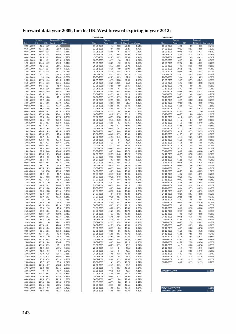
143




Forward DK West

Log change Date

System Price CfD


System Price CfD


02-01-2009 40.5 11.9 52.43 11-05-2009 43 9.88 52.88 -0.51% 11-09-2009 40.6 8.9 49.5 0.24%05-01-2009 40.75 12.1 52.88 0.85% 12-05-2009 43.4 9.85 53.25 0.70% 14-09-2009 40.02 8.93 48.95 -1.12%06-01-2009 43.05 11.8 54.85 3.66% 13-05-2009 42.85 9.7 52.55 -1.32% 15-09-2009 40.48 8.75 49.23 0.57%07-01-2009 42.85 11.8 54.65 -0.37% 14-05-2009 42.7 9.95 52.65 0.19% 16-09-2009 40.4 8.75 49.15 -0.16%08-01-2009 41.5 12.2 53.68 -1.79% 15-05-2009 42.85 10.03 52.88 0.44% 17-09-2009 40.23 8.9 49.13 -0.04%09-01-2009 41.1 12.1 53.23 -0.84% 18-05-2009 42.9 10 52.9 0.04% 18-09-2009 40.3 8.8 49.1 -0.06%12-01-2009 40.45 11.9 52.33 -1.71% 19-05-2009 43.25 10 53.25 0.66% 21-09-2009 39.92 8.8 48.72 -0.78%13-01-2009 40.6 11.4 51.95 -0.73% 20-05-2009 43.73 10.05 53.78 0.99% 22-09-2009 40.1 8.95 49.05 0.68%14-01-2009 40.25 11.4 51.68 -0.52% 22-05-2009 43.18 9.9 53.08 -1.31% 23-09-2009 39.75 8.93 48.68 -0.76%15-01-2009 40.18 11.5 51.71 0.06% 25-05-2009 42.75 10.05 52.8 -0.53% 24-09-2009 39.45 8.88 48.33 -0.72%16-01-2009 40.1 11.7 51.8 0.17% 26-05-2009 42.2 10.05 52.25 -1.05% 25-09-2009 39.1 8.95 48.05 -0.58%19-01-2009 39 11.4 50.43 -2.68% 27-05-2009 42.85 10.05 52.9 1.24% 28-09-2009 39.4 8.9 48.3 0.52%20-01-2009 37.75 11.4 49.18 -2.51% 28-05-2009 42.9 10.08 52.98 0.15% 29-09-2009 39.5 8.95 48.45 0.31%21-01-2009 37.75 11.6 49.35 0.35% 29-05-2009 43.25 10.05 53.3 0.60% 30-09-2009 39.7 8.88 48.58 0.27%22-01-2009 37.55 11.4 48.9 -0.92% 02-06-2009 43.55 9.9 53.45 0.28% 01-10-2009 39.8 8.9 48.7 0.25%23-01-2009 37.4 11.6 48.95 0.10% 03-06-2009 43.05 9.1 52.15 -2.46% 02-10-2009 39.2 8.88 48.08 -1.28%26-01-2009 38.63 10.9 49.48 1.08% 04-06-2009 43.05 9.03 52.08 -0.13% 05-10-2009 39.38 8.85 48.23 0.31%27-01-2009 38.15 11 49.13 -0.71% 05-06-2009 43.35 8.83 52.18 0.19% 06-10-2009 39.85 8.8 48.65 0.87%28-01-2009 38.3 10.8 49.1 -0.06% 08-06-2009 42.99 8.95 51.94 -0.46% 07-10-2009 40.15 8.75 48.9 0.51%29-01-2009 38.2 10.8 49 -0.20% 09-06-2009 42.95 8.83 51.78 -0.31% 08-10-2009 39.9 8.88 48.78 -0.25%30-01-2009 39.1 10.6 49.73 1.48% 10-06-2009 42.95 8.65 51.6 -0.35% 09-10-2009 40.15 8.83 48.98 0.41%02-02-2009 38.1 11 49.13 -1.21% 11-06-2009 42.85 8.63 51.48 -0.23% 12-10-2009 41.18 8.73 49.91 1.88%03-02-2009 38.3 10.6 48.88 -0.51% 12-06-2009 42.4 8.48 50.88 -1.17% 13-10-2009 41.1 8.65 49.75 -0.32%04-02-2009 38.05 10.2 48.25 -1.30% 15-06-2009 41.25 8.4 49.65 -2.45% 14-10-2009 41.35 8.65 50 0.50%05-02-2009 38.23 10.4 48.61 0.74% 16-06-2009 41.8 8.35 50.15 1.00% 15-10-2009 40.85 8.6 49.45 -1.11%06-02-2009 38.3 10.4 48.73 0.25% 17-06-2009 40.53 8.38 48.91 -2.50% 16-10-2009 41.2 8.75 49.95 1.01%09-02-2009 39.6 10 49.63 1.83% 18-06-2009 40.75 8.38 49.13 0.45% 19-10-2009 41.2 8.7 49.9 -0.10%10-02-2009 39.6 9.93 49.53 -0.20% 19-06-2009 41.05 8.3 49.35 0.45% 20-10-2009 41.9 8.58 50.48 1.16%11-02-2009 38.75 9.73 48.48 -2.14% 22-06-2009 39.9 8.13 48.03 -2.71% 21-10-2009 41.85 8.45 50.3 -0.36%12-02-2009 37.8 9.5 47.3 -2.46% 23-06-2009 40.35 8.1 48.45 0.87% 22-10-2009 41.7 8.65 50.35 0.10%13-02-2009 37.85 9.5 47.35 0.11% 24-06-2009 40.15 8.48 48.63 0.37% 23-10-2009 41.8 8.55 50.35 0.00%16-02-2009 37.55 9.75 47.3 -0.11% 25-06-2009 40.48 8.35 48.83 0.41% 26-10-2009 41.65 8.7 50.35 0.00%17-02-2009 36.7 9.4 46.1 -2.57% 26-06-2009 41.13 8.43 49.56 1.48% 27-10-2009 41.3 9.25 50.55 0.40%18-02-2009 36.84 9.5 46.34 0.52% 29-06-2009 41.5 8.4 49.9 0.68% 28-10-2009 41.35 9.15 50.5 -0.10%19-02-2009 36.5 9.13 45.63 -1.54% 30-06-2009 41.3 8.4 49.7 -0.40% 29-10-2009 41.6 8.9 50.5 0.00%20-02-2009 35.65 9.08 44.73 -1.99% 01-07-2009 41.1 8.48 49.58 -0.24% 30-10-2009 41.6 8.8 50.4 -0.20%23-02-2009 33.8 9.48 43.28 -3.30% 02-07-2009 40.45 8.48 48.93 -1.32% 02-11-2009 41.6 8.8 50.4 0.00%24-02-2009 33.6 9.48 43.08 -0.46% 03-07-2009 40.3 8.48 48.78 -0.31% 03-11-2009 40.8 8.88 49.68 -1.44%25-02-2009 33.38 9.5 42.88 -0.47% 06-07-2009 39.75 8.48 48.23 -1.13% 04-11-2009 40.85 8.98 49.83 0.30%26-02-2009 34.4 9.5 43.9 2.35% 07-07-2009 40.15 8.58 48.73 1.03% 05-11-2009 41 8.35 49.35 -0.97%27-02-2009 33.6 9.7 43.3 -1.38% 08-07-2009 40.1 8.58 48.68 -0.10% 06-11-2009 41.15 8.38 49.53 0.36%02-03-2009 32.55 9.58 42.13 -2.74% 09-07-2009 40.23 8.95 49.18 1.02% 09-11-2009 40.75 8.5 49.25 -0.57%03-03-2009 33.1 9.8 42.9 1.81% 10-07-2009 40.25 8.58 48.83 -0.71% 10-11-2009 40.85 8.6 49.45 0.41%04-03-2009 34.75 9.3 44.05 2.65% 13-07-2009 40.25 8.48 48.73 -0.21% 11-11-2009 41.1 8.7 49.8 0.71%05-03-2009 34 9.58 43.58 -1.07% 14-07-2009 40.5 8.48 48.98 0.51% 12-11-2009 40.25 8.8 49.05 -1.52%06-03-2009 34.2 9.5 43.7 0.27% 15-07-2009 40.45 8.48 48.93 -0.10% 13-11-2009 40.2 8.75 48.95 -0.20%09-03-2009 35.1 9.58 44.68 2.22% 16-07-2009 40.38 8.48 48.86 -0.14% 16-11-2009 40.28 8.73 49.01 0.12%10-03-2009 36.15 9.75 45.9 2.69% 17-07-2009 40.4 8.48 48.88 0.04% 17-11-2009 40.41 8.68 49.09 0.16%11-03-2009 35.25 10 45.25 -1.43% 20-07-2009 40.2 8.53 48.73 -0.31% 18-11-2009 40.8 8.65 49.45 0.73%12-03-2009 34.6 10.1 44.65 -1.33% 21-07-2009 40.75 8.48 49.23 1.02% 19-11-2009 40.6 8.58 49.18 -0.55%13-03-2009 35.25 10.4 45.63 2.17% 22-07-2009 40.5 8.48 48.98 -0.51% 20-11-2009 40.4 8.55 48.95 -0.47%16-03-2009 35.4 10.8 46.15 1.13% 23-07-2009 40.38 8.48 48.86 -0.25% 23-11-2009 40.43 8.5 48.93 -0.04%17-03-2009 36.2 10 46.23 0.17% 24-07-2009 40.4 8.48 48.88 0.04% 24-11-2009 40.05 8.53 48.58 -0.72%18-03-2009 35.9 10.3 46.18 -0.11% 27-07-2009 40.35 8.53 48.88 0.00% 25-11-2009 39.85 8.55 48.4 -0.37%19-03-2009 37 10 47 1.76% 28-07-2009 40.2 8.53 48.73 -0.31% 26-11-2009 40.2 8.6 48.8 0.82%20-03-2009 37.5 10 47.5 1.06% 29-07-2009 40.4 8.53 48.93 0.41% 27-11-2009 40.13 8.63 48.76 -0.08%23-03-2009 39.15 9.98 49.13 3.37% 30-07-2009 40.7 8.53 49.23 0.61% 30-11-2009 40 8.6 48.6 -0.33%24-03-2009 38.3 10 48.3 -1.70% 31-07-2009 40.8 8.53 49.33 0.20% 01-12-2009 40.7 8.18 48.88 0.57%25-03-2009 37.9 10.3 48.15 -0.31% 03-08-2009 41.25 8.53 49.78 0.91% 02-12-2009 40.35 8.05 48.4 -0.99%26-03-2009 38.95 10 48.98 1.71% 04-08-2009 41.3 8.53 49.83 0.10% 03-12-2009 40.5 8.38 48.88 0.99%27-03-2009 38.08 10.2 48.26 -1.48% 05-08-2009 41.45 8.58 50.03 0.40% 04-12-2009 40.75 8.18 48.93 0.10%30-03-2009 37.2 10 47.23 -2.16% 06-08-2009 41.5 8.58 50.08 0.10% 07-12-2009 41.35 7.73 49.08 0.31%31-03-2009 37.41 10 47.41 0.38% 07-08-2009 41.33 8.58 49.91 -0.34% 08-12-2009 40.95 7.9 48.85 -0.47%01-04-2009 37.75 10.1 47.83 0.88% 10-08-2009 41.25 8.58 49.83 -0.16% 09-12-2009 40.75 8.05 48.8 -0.10%02-04-2009 39.25 10.4 49.63 3.69% 11-08-2009 40.75 8.6 49.35 -0.97% 10-12-2009 40.9 8.08 48.98 0.37%03-04-2009 39.6 10.1 49.68 0.10% 12-08-2009 40.65 8.6 49.25 -0.20% 11-12-2009 41.35 8.03 49.38 0.81%06-04-2009 39.75 10.1 49.8 0.24% 13-08-2009 41.08 8.63 49.71 0.93% 14-12-2009 41.65 7.85 49.5 0.24%07-04-2009 39.2 10 49.2 -1.21% 14-08-2009 41.63 8.65 50.28 1.14% 15-12-2009 41.8 7.98 49.78 0.56%08-04-2009 39.25 9.98 49.23 0.06% 17-08-2009 40.95 8.38 49.33 -1.91% 16-12-2009 41.65 7.95 49.6 -0.36%14-04-2009 40.25 9.8 50.05 1.65% 18-08-2009 40.7 8.48 49.18 -0.30% 17-12-2009 41.28 7.98 49.26 -0.69%15-04-2009 40.35 9.75 50.1 0.10% 19-08-2009 40.85 8.35 49.2 0.04% 18-12-2009 41.5 8.08 49.58 0.65%16-04-2009 41.2 9.75 50.95 1.68% 20-08-2009 41.1 8.4 49.5 0.61% 21-12-2009 41.5 7.95 49.45 -0.26%17-04-2009 42.3 9.7 52 2.04% 21-08-2009 41.2 8.4 49.6 0.20% 22-12-2009 41.9 8.55 50.45 2.00%20-04-2009 40.9 9.75 50.65 -2.63% 24-08-2009 40.9 8.38 49.28 -0.65% 23-12-2009 42.7 8.33 51.03 1.14%21-04-2009 40.2 9.75 49.95 -1.39% 25-08-2009 40.9 8.5 49.4 0.24% 28-12-2009 43.01 8.25 51.26 0.45%22-04-2009 40.6 9.78 50.38 0.86% 26-08-2009 40.8 8.55 49.35 -0.10% 29-12-2009 42.8 8.13 50.93 -0.65%23-04-2009 40.7 9.7 50.4 0.04% 27-08-2009 41 8.73 49.73 0.77% 30-12-2009 43.2 8.13 51.33 0.78%24-04-2009 41.18 9.7 50.88 0.95% 28-08-2009 41.45 8.75 50.2 0.94%27-04-2009 39.8 9.65 49.45 -2.85% 31-08-2009 41 8.63 49.63 -1.14%28-04-2009 40 9.7 49.7 0.50% 01-09-2009 40.75 8.75 49.5 -0.26% Annual Vol. 2009 17.80%29-04-2009 40.45 9.68 50.13 0.86% 02-09-2009 40.5 8.65 49.15 -0.71%30-04-2009 40.9 9.65 50.55 0.83% 03-09-2009 40.88 8.75 49.63 0.97%04-05-2009 41.5 9.75 51.25 1.38% 04-09-2009 40.55 8.8 49.35 -0.57%05-05-2009 41.55 9.8 51.35 0.19% 07-09-2009 40.35 8.8 49.15 -0.41%06-05-2009 42.25 9.8 52.05 1.35% 08-09-2009 40.75 8.8 49.55 0.81%07-05-2009 43.13 9.7 52.83 1.49% 09-09-2009 40.8 8.73 49.53 -0.04% Daily vol. 2007-2009 1.09%08-05-2009 43.3 9.85 53.15 0.60% 10-09-2009 40.5 8.88 49.38 -0.30% Annual vol. 2007-2009 17.27%

144

Appendix 14 Implied Volatilities

As the underlying asset of electricity options is forwards, the Black 76 model should be used. This

is basically a Black-Scholes model yielding no interests, as the forwards requires no upfront

payment, hence carries no cost of financing (Pilipovic, p. 279).

Formula A. 3 Black Model (Also known as Black 76 model)

CP = Fe−rTN(d1) − EXe−rTN(d2)

d1 =ln � F

EX � + �σ2

2 �T

σ√T

d2 = d1 − σ√T

𝑪𝒑: Call price

𝒓: Risk-free rate

𝑻: Time to maturity

𝝈: Volatility of underlying asset

𝑵(𝒅): Cumulative probability density function

𝑭: Price of forward


Source: Pilipovic 2007: 279

By use of the above formula in Excel’s solver function, the volatility implied in the traded option

prices is estimated. This can be seen in the table below, and the calculations can be found on the

attached Data CD.

Table A. 11 Implied Volatility Nord Pool and European Energy Exchange 3

Source: System Price: www.nordpool.dk, SPAN file: SPAN_000852, Phelix Price: www.eex.com

Peer 1: Peer 2: Peer 3:Exchange: Nord Pool European Energy Exchange European Energy Exchange

Market: System Price Phelix Price Phelix Price

Option: ENOC45YR-11 C5700 for Cal-11 C6000 for Cal-13

Description:Call option for ENOYR-11, excercise price 45€/MWh

Call option for Cal-11, excercise price 57€/MWh

Call option for Cal-13, excercise price 60€/MWh

Underlying Asset: ENOYR-11 Baseload Year Futures Cal-11 Baseload Year Futures Cal-13

Description:Forward on 1 MWh delivered throughout 2011 (System

Future on 1 MWh delivered throughout 2011 (Phelix Price)

Future on 1 MWh delivered throughout 2013 (Phelix Price)

Date of Analysis: 30-12-2009 30-12-2009 30-12-2009Exercise Date: 18-12-2010 28-12-2010 21-12-2012Time to Maturity: (T) ,97 Years ,99 Years 2,98 YearsRisk-free: (r) * 2,01% 2,01% 2,01%

Price of Underlying Asset: (F) 42,15 €/MWh 51,54 €/MWh 61,44 €/MWh

Exercise Price: (K) 45,00 €/MWh 57,00 €/MWh 60,00 €/MWh

d1 -0,094402288 -0,381813282 0,240582808d2 -0,373854788 -0,589209222 -0,102210734N(d1) 0,462394799 0,351299933 0,595060762N(d2) 0,354256178 0,277860466 0,459294704

Empirical Call Price: (C p ) 3,480€ 2,223€ 8,479€ Call Price (Black Model) : 3,479999713 2,222999755 8,478999915Difference: 2,86825E-07 2,45179E-07 8,53043E-08

Volatility (Found by solver) 28,42% 20,80% 19,86%

* The applied risk free-rate is the effective rate of a 2 year danish government bond (Nationalbanken)

http://www.nordpool.dk/

http://www.eex.com/

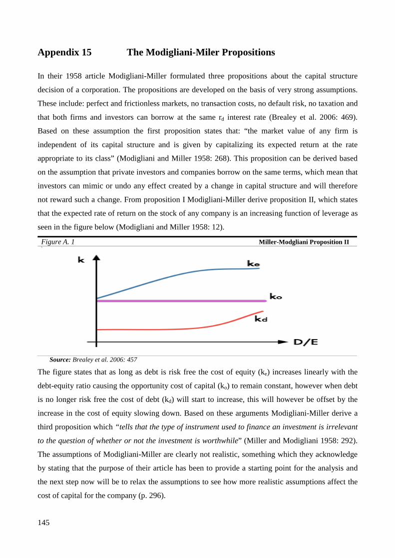
145

Appendix 15 The Modigliani-Miler Propositions

In their 1958 article Modigliani-Miller formulated three propositions about the capital structure

decision of a corporation. The propositions are developed on the basis of very strong assumptions.

These include: perfect and frictionless markets, no transaction costs, no default risk, no taxation and

that both firms and investors can borrow at the same rd interest rate (Brealey et al. 2006: 469).

Based on these assumption the first proposition states that: “the market value of any firm is

independent of its capital structure and is given by capitalizing its expected return at the rate

appropriate to its class” (Modigliani and Miller 1958: 268). This proposition can be derived based

on the assumption that private investors and companies borrow on the same terms, which mean that

investors can mimic or undo any effect created by a change in capital structure and will therefore

not reward such a change. From proposition I Modigliani-Miller derive proposition II, which states

that the expected rate of return on the stock of any company is an increasing function of leverage as

seen in the figure below (Modigliani and Miller 1958: 12).

Figure A. 1 Miller-Modgliani Proposition II

3


The figure states that as long as debt is risk free the cost of equity (ke) increases linearly with the

debt-equity ratio causing the opportunity cost of capital (ko) to remain constant, however when debt

is no longer risk free the cost of debt (kd) will start to increase, this will however be offset by the

increase in the cost of equity slowing down. Based on these arguments Modigliani-Miller derive a

third proposition which “tells that the type of instrument used to finance an investment is irrelevant

to the question of whether or not the investment is worthwhile” (Miller and Modigliani 1958: 292).

The assumptions of Modigliani-Miller are clearly not realistic, something which they acknowledge

by stating that the purpose of their article has been to provide a starting point for the analysis and

the next step now will be to relax the assumptions to see how more realistic assumptions affect the

cost of capital for the company (p. 296).

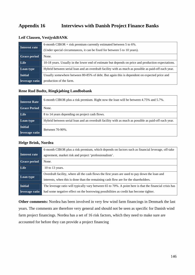
146

Appendix 16 Interviews with Danish Project Finance Banks

Leif Clausen, VestjyskBANK

Interest rate 6-month CIBOR + risk premium currently estimated between 5 to 6%.

(Under special circumstances, it can be fixed for between 5 to 10 years).

Grace period None.

Life 10-18 years. Usually in the lower end of estimate but depends on price and production expectations.

Loan type Hybrid between serial loan and an overdraft facility with as much as possible as paid-off each year.

Initial

leverage ratio

Usually somewhere between 80-85% of debt. But again this is dependent on expected price and

production of the farm.

Rene Rud Budtz, Ringkjøbing Landbobank

Interest Rate 6-month CIBOR plus a risk premium. Right now the loan will be between 4.75% and 5.7%.

Grace Period None.

Life 8 to 14 years depending on project cash flows.

Loan type Hybrid between serial loan and an overdraft facility with as much as possible as paid-off each year.

Initial

leverage ratio Between 70-90%.

Helge Brink, Nordea

Interest rate 6-month CIBOR plus a risk premium, which depends on factors such as financial leverage, off-take

agreement, market risk and project ‘professionalism’.

Grace period None.

Life 10 to 13 years.

Loan type Overdraft facility, where all the cash flows the first years are used to pay down the loan and

interests, when this is done than the remaining cash flow are for the shareholders.

Initial

leverage ratio

The leverage ratio will typically vary between 65 to 70%. A point here is that the financial crisis has

had some negative effect on the borrowing possibilities as credit has become tighter.

Other comments: Nordea has been involved in very few wind farm financings in Denmark the last

years. The comments are therefore very general and should not be seen as specific for Danish wind

farm project financings. Nordea has a set of 16 risk factors, which they need to make sure are

accounted for before they can provide a project financing

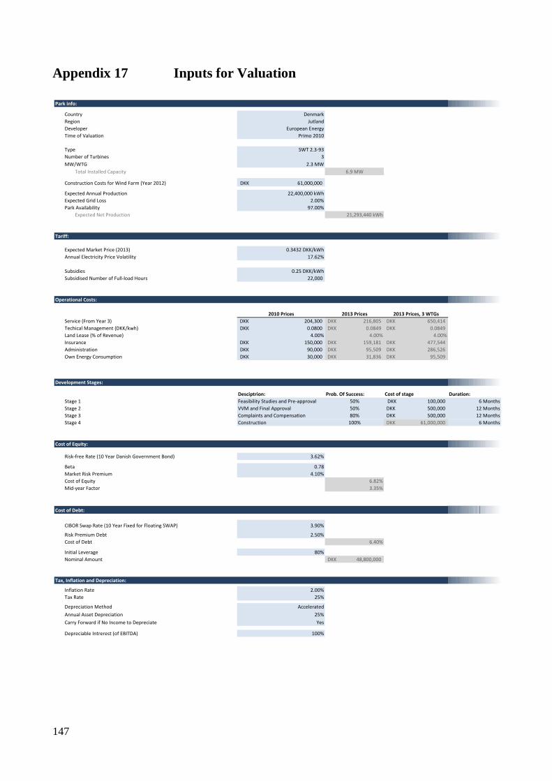
147

Appendix 17 Inputs for Valuation

Park info:

CountryRegionDeveloperTime of Valuation

TypeNumber of TurbinesMW/WTG

Total Installed Capacity 6.9 MW

Construction Costs for Wind Farm (Year 2012)

Expected Annual ProductionExpected Grid LossPark Availability

Expected Net Production 21,293,440 kWh

Tariff:

Expected Market Price (2013)Annual Electricity Price Volatility

SubsidiesSubsidised Number of Full-load Hours

Operational Costs:

2013 Prices 2013 Prices, 3 WTGsService (From Year 3) 216,805DKK 650,414DKK Techical Management (DKK/kwh) 0.0849DKK 0.0849DKK Land Lease (% of Revenue) 4.00% 4.00%Insurance 159,181DKK 477,544DKK Administration 95,509DKK 286,526DKK Own Energy Consumption 31,836DKK 95,509DKK

Development Stages:

Desciptrion: Prob. Of Success: Cost of stage Duration:Stage 1 Feasibility Studies and Pre-approval 50% 100,000DKK 6 MonthsStage 2 VVM and Final Approval 50% 500,000DKK 12 MonthsStage 3 Complaints and Compensation 80% 500,000DKK 12 MonthsStage 4 Construction 100% 61,000,000DKK 6 Months

Cost of Equity:

Risk-free Rate (10 Year Danish Government Bond)

BetaMarket Risk PremiumCost of Equity 6.82%Mid-year Factor 3.35%

Cost of Debt:

CIBOR Swap Rate (10 Year Fixed for Floating SWAP)

Risk Premium DebtCost of Debt 6.40%

Initial LeverageNominal Amount 48,800,000DKK

Tax, Inflation and Depreciation:

Inflation RateTax Rate

Depreciation MethodAnnual Asset DepreciationCarry Forward if No Income to Depreciate

Depreciable Intrerest (of EBITDA)

25%

100%

Yes

80%

25%2.00%

Accelerated

32.3 MW

61,000,000DKK

22,400,000 kWh

2.50%

4.10%

3.90%

150,000DKK 90,000DKK 30,000DKK

3.62%

22,000

204,300DKK 0.0800DKK

2010 Prices

0.78

DenmarkJutland

European EnergyPrimo 2010

SWT 2.3-93

4.00%

2.00%97.00%

0.3432 DKK/kWh17.62%

0.25 DKK/kWh

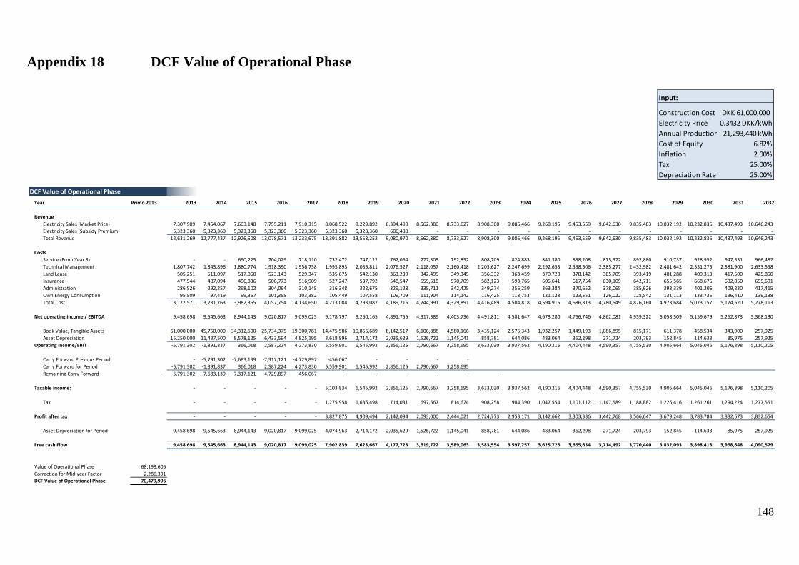
148

Appendix 18 DCF Value of Operational Phase

Input:

Construction Cost 61,000,000DKK Electricity Price 0.3432 DKK/kWhAnnual Production 21,293,440 kWhCost of Equity 6.82%Inflation 2.00%Tax 25.00%Depreciation Rate 25.00%

DCF Value of Operational PhaseYear Primo 2013 2013 2014 2015 2016 2017 2018 2019 2020 2021 2022 2023 2024 2025 2026 2027 2028 2029 2030 2031 2032

RevenueElectricity Sales (Market Price) 7,307,909 7,454,067 7,603,148 7,755,211 7,910,315 8,068,522 8,229,892 8,394,490 8,562,380 8,733,627 8,908,300 9,086,466 9,268,195 9,453,559 9,642,630 9,835,483 10,032,192 10,232,836 10,437,493 10,646,243 Electricity Sales (Subsidy Premium) 5,323,360 5,323,360 5,323,360 5,323,360 5,323,360 5,323,360 5,323,360 686,480 - - - - - - - - - - - - Total Revenue 12,631,269 12,777,427 12,926,508 13,078,571 13,233,675 13,391,882 13,553,252 9,080,970 8,562,380 8,733,627 8,908,300 9,086,466 9,268,195 9,453,559 9,642,630 9,835,483 10,032,192 10,232,836 10,437,493 10,646,243

CostsService (From Year 3) - - 690,225 704,029 718,110 732,472 747,122 762,064 777,305 792,852 808,709 824,883 841,380 858,208 875,372 892,880 910,737 928,952 947,531 966,482 Technical Management 1,807,742 1,843,896 1,880,774 1,918,390 1,956,758 1,995,893 2,035,811 2,076,527 2,118,057 2,160,418 2,203,627 2,247,699 2,292,653 2,338,506 2,385,277 2,432,982 2,481,642 2,531,275 2,581,900 2,633,538 Land Lease 505,251 511,097 517,060 523,143 529,347 535,675 542,130 363,239 342,495 349,345 356,332 363,459 370,728 378,142 385,705 393,419 401,288 409,313 417,500 425,850 Insurance 477,544 487,094 496,836 506,773 516,909 527,247 537,792 548,547 559,518 570,709 582,123 593,765 605,641 617,754 630,109 642,711 655,565 668,676 682,050 695,691 Administration 286,526 292,257 298,102 304,064 310,145 316,348 322,675 329,128 335,711 342,425 349,274 356,259 363,384 370,652 378,065 385,626 393,339 401,206 409,230 417,415 Own Energy Consumption 95,509 97,419 99,367 101,355 103,382 105,449 107,558 109,709 111,904 114,142 116,425 118,753 121,128 123,551 126,022 128,542 131,113 133,735 136,410 139,138 Total Cost 3,172,571 3,231,763 3,982,365 4,057,754 4,134,650 4,213,084 4,293,087 4,189,215 4,244,991 4,329,891 4,416,489 4,504,818 4,594,915 4,686,813 4,780,549 4,876,160 4,973,684 5,073,157 5,174,620 5,278,113

Net operating income / EBITDA 9,458,698 9,545,663 8,944,143 9,020,817 9,099,025 9,178,797 9,260,165 4,891,755 4,317,389 4,403,736 4,491,811 4,581,647 4,673,280 4,766,746 4,862,081 4,959,322 5,058,509 5,159,679 5,262,873 5,368,130

Book Value, Tangible Assets 61,000,000 45,750,000 34,312,500 25,734,375 19,300,781 14,475,586 10,856,689 8,142,517 6,106,888 4,580,166 3,435,124 2,576,343 1,932,257 1,449,193 1,086,895 815,171 611,378 458,534 343,900 257,925 Asset Depreciation 15,250,000 11,437,500 8,578,125 6,433,594 4,825,195 3,618,896 2,714,172 2,035,629 1,526,722 1,145,041 858,781 644,086 483,064 362,298 271,724 203,793 152,845 114,633 85,975 257,925

Operating income/EBIT -5,791,302 -1,891,837 366,018 2,587,224 4,273,830 5,559,901 6,545,992 2,856,125 2,790,667 3,258,695 3,633,030 3,937,562 4,190,216 4,404,448 4,590,357 4,755,530 4,905,664 5,045,046 5,176,898 5,110,205

Carry Forward Previous Period - -5,791,302 -7,683,139 -7,317,121 -4,729,897 -456,067 - - - - Carry Forward for Period -5,791,302 -1,891,837 366,018 2,587,224 4,273,830 5,559,901 6,545,992 2,856,125 2,790,667 3,258,695 Remaining Carry Forward - -5,791,302 -7,683,139 -7,317,121 -4,729,897 -456,067 - - - - - -

Taxable income: - - - - - 5,103,834 6,545,992 2,856,125 2,790,667 3,258,695 3,633,030 3,937,562 4,190,216 4,404,448 4,590,357 4,755,530 4,905,664 5,045,046 5,176,898 5,110,205

Tax - - - - - 1,275,958 1,636,498 714,031 697,667 814,674 908,258 984,390 1,047,554 1,101,112 1,147,589 1,188,882 1,226,416 1,261,261 1,294,224 1,277,551

Profit after tax - - - - - 3,827,875 4,909,494 2,142,094 2,093,000 2,444,021 2,724,773 2,953,171 3,142,662 3,303,336 3,442,768 3,566,647 3,679,248 3,783,784 3,882,673 3,832,654

Asset Depreciation for Period 9,458,698 9,545,663 8,944,143 9,020,817 9,099,025 4,074,963 2,714,172 2,035,629 1,526,722 1,145,041 858,781 644,086 483,064 362,298 271,724 203,793 152,845 114,633 85,975 257,925

Free cash Flow 9,458,698 9,545,663 8,944,143 9,020,817 9,099,025 7,902,839 7,623,667 4,177,723 3,619,722 3,589,063 3,583,554 3,597,257 3,625,726 3,665,634 3,714,492 3,770,440 3,832,093 3,898,418 3,968,648 4,090,579

Value of Operational Phase 68,193,605Correction for Mid-year Factor 2,286,391DCF Value of Operational Phase 70,479,996

149

Appendix 19 Value of Financial Side Effects

Input:

Cost of Debt 6.40%Leverage Ratio 80%Principal 48,800,000DKK Tax 25.00%

Financial Side Effects

Year Primo 2013 2013 2014 2015 2016 2017 2018 2019 2020 2021 2022 2023 2024 2025 2026 2027 2028 2029 2030 2031 2032

Interest Expense 3,120,760 2,715,449 2,278,657 1,852,399 1,393,978 901,241 371,891 - - - - - - - - - - - - -

Remaining Principal Primo 48,800,000 42,462,062 35,631,848 28,966,361 21,797,943 14,092,896 5,815,339 - - - - - - - - - - - - - Installment 6,337,938 6,830,214 6,665,486 7,168,419 7,705,047 7,001,598 5,815,339 - - - - - - - - - - - - - Remaining Principal Ultimo 48,800,000 42,462,062 35,631,848 28,966,361 21,797,943 14,092,896 7,091,297 - - - - - - - - - - - - - -

Tax - - - - - 1,275,958 1,636,498 714,031 697,667 814,674 908,258 984,390 1,047,554 1,101,112 1,147,589 1,188,882 1,226,416 1,261,261 1,294,224 1,277,551

ITS Carry Forward Primo - 780,190 1,459,052 2,028,716 2,491,816 2,840,311 1,789,662 246,137 - - - - - - - - - - - - ITS Generated in Period 780,190 678,862 569,664 463,100 348,495 225,310 92,973 - - - - - - - - - - - - - Cash Flow from ITS - - - - - -1,275,958 -1,636,498 -246,137 - - - - - - - - - - - - ITS Carry Forward Ultimo - 780,190 1,459,052 2,028,716 2,491,816 2,840,311 1,789,662 246,137 - - - - - - - - - - - - -

Remaining Principal Ultimo 42,462,062 35,631,848 28,966,361 21,797,943 14,092,896 7,091,297 - - - - - - - - - - - - - - Cash Flow from ITS - - - - - 1,275,958 1,636,498 246,137 - - - - - - - - - - - - Remaining Principal Ultimo (Corrected for ITS Cash Flow)

48,800,000 42,462,062 35,631,848 28,966,361 21,797,943 14,092,896 5,815,339 - - - - - - - - - - - - - -

Cash Flow from Interest Tax Shield - - - - - 1,275,958 1,636,498 246,137 - - - - - - - - - - - -

PV, Interest Tax Shield 2,089,944Mid-year Factor 65,790 PV, Financial Side Effects: 2,155,734

150

Appendix 20 Annual Wind Distribution

The available wind resources of a wind farm will vary from year to year, but as the annual wind

resources are expected to be normally distributed. Therefore it is reasonable to use a fixed

production for all 20 years of the operational phase., especially as the expected production is

estimated as a so-called “normal-year”, so that the estimate is adjusted to match the long term

expectations of a particular site by use of the so-called wind-index.

The wind index is a relative measure of the available wind resources in different years.86 The wind

index is estimated from the actual production of wind turbines all around the country, and is a

relative measure of the annual deviation in wind resources from the historical average (year 1979-

2010). An average year is wind index 100 hence an index year 110 is 10% better than expected. The

distribution of wind years over the past 30 years can be seen from the figure below.

Figure A. 2 Annual Wind Index (1979-2010)

Data: www.vindstat.dk

As the expected production estimate of the wind farm, in our case 22,400,000 kWh, is adjusted to

be an index 100 estimate, this is what we can expect to be the average production over the 20 year

operational life time of the wind farm.

86 The distribution of the annual production from the wind index should not be confused with the so-called power-curve which determines the annual production from the average wind speed, as this is typically accepted to follow a Weibull-distribution. Holtinnen and Nørregaard, A Multi-Turbine Power Curve Approach, p. 4.

80

85

90

95

100

105

110

115

120

Inde

x

Annual Wind IndexAnnual wind indexAverage 100

wind farm

Documents