willingness to pay for clean air: evidence from air purifier … · 2020-03-11 · air pollution...
TRANSCRIPT

Willingness to Pay for Clean Air:
Evidence from Air Purifier Markets in China
Koichiro Ito Shuang Zhang
University of Chicago & NBER University of Colorado Boulder
1 / 61

Air pollution is very severe in developing countries
Global Annual Average PM2.5 Grids from MODIS and MISR Aerosol Optical Depth (AOD), 2010Satellite-Derived Environmental Indicators
Global Annual PM2.5 Grids from MODIS and MISR Aerosol Optical Depth (AOD) data sets provide annual“snap shots” of particulate matter 2.5 micrometers or smaller in diameter from 2001–2010. Exposure to fineparticles is associated with premature death as well as increased morbidity from respiratory andcardiovascular disease, especially in the elderly, young children, and those already suffering from theseillnesses. The grids were derived from Moderate Resolution Imaging Spectroradiometer (MODIS) and Multi-angle Imaging SpectroRadiometer (MISR) Aerosol Optical Depth (AOD) data. The raster grids have a grid cellresolution of 30 arc-minutes (0.5 degree or approximately 50 sq. km at the equator) and cover the world from70°N to 60°S latitude. The grids were produced by researchers at Battelle Memorial Institute in collaborationwith the Center for International Earth Science Information Network/Columbia University under a NASAResearch Opportunities in Space and Earth Sciences (ROSES) project entitled “Using Satellite Data toDevelop Environmental Indicators.”
Data Source: Battelle Memorial Institute, and Center for International Earth Science Information Network (CIESIN)/Columbia University. 2013. GlobalAnnual Average PM2.5 Grids from MODIS and MISR Aerosol Optical Depth (AOD), 2001–2010. Palisades, NY: NASA Socioeconomic Data andApplications Center (SEDAC). http://sedac.ciesin.columbia.edu/data/set/sdei-global-annual-avg-pm2-5-2001-2010.
Robinson Projection
Particulate Matter (PM2.5)(units: µg/m3)
0 5 10 15 20 50 >80
© 2013. The Trustees of Columbia University in the City of New York.
Map Credit: CIESIN Columbia University, April 2013.
This document is licensed under aCreative Commons 3.0 Attribution Licensehttp://creativecommons.org/licenses/by/3.0/

Air pollution is very severe in developing countries
Source: Chianews.com
3/ 61

Research question: How much are people willing to pay for
clean air in developing countries?
• Severe air pollution ) Health and economic costsI Jayachandran (2009); Greenstone and Hanna (2014); Hanna and Oliva (2015)
• High costs of pollution ; Current env. regulations are not optimalI Willingness-to-pay is a key parameter to determine optimal
environmental regulation (Greenstone and Jack, 2014)
• Yet, limited evidence on WTP for clean air in developing countriesI Data: Hard to obtain data required to estimate WTPI Identification problems: Hard to have exogenous variation
4 / 61

This paper
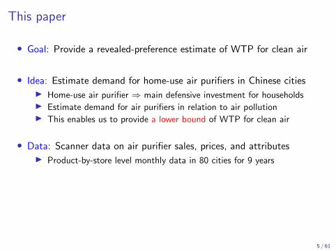
• Goal: Provide a revealed-preference estimate of WTP for clean air
• Idea: Estimate demand for home-use air purifiers in Chinese citiesI Home-use air purifier ) main defensive investment for householdsI Estimate demand for air purifiers in relation to air pollutionI This enables us to provide a lower bound of WTP for clean air
• Data: Scanner data on air purifier sales, prices, and attributesI Product-by-store level monthly data in 80 cities for 9 years
• Quasi-experimental variation in pollution levels and purifier pricesI The Huai River Policy ) A natural experiment to air pollutionI Road distance from factory/port to market ) IV for purifier prices
5 / 61

This paper
• Goal: Provide a revealed-preference estimate of WTP for clean air
• Idea: Estimate demand for home-use air purifiers in Chinese citiesI Home-use air purifier ) main defensive investment for householdsI Estimate demand for air purifiers in relation to air pollutionI This enables us to provide a lower bound of WTP for clean air
• Data: Scanner data on air purifier sales, prices, and attributesI Product-by-store level monthly data in 80 cities for 9 years
• Quasi-experimental variation in pollution levels and purifier pricesI The Huai River Policy ) A natural experiment to air pollutionI Road distance from factory/port to market ) IV for purifier prices
5 / 61

Huai river policy created long-run variation in air pollutionFigure 1: Huai River Boundary and City Locations
Note: The line in the middle of the map shows the Huai River-Qinling boundary.
46
• Government built coal-based centralized heating in the North in 1950’s
• Created plausibly exogenous, long-run variation in air pollution
6 / 61

A boiler house in an apartment complex (Shenyang)
Source: Chianews.com
7/ 61

PM10 by distance to the Huai River border (raw data)
7080
9010
011
012
013
0PM
10
-4 -3.5 -3 -2.5 -2 -1.5 -1 -.5 0 .5 1 1.5 2 2.5 3 3.5 4Distance North to the Huai River (100 miles)
• Note: In the US, average PM10 was 55 ug/m3 in 2014 (it was 85 in 1990)8 / 61
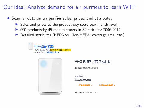
Our idea: Analyze demand for air purifiers to learn WTP
• Scanner data on air purifier sales, prices, and attributesI Sales and prices at the product-city-store-year-month levelI 690 products by 45 manufacturers in 80 cities for 2006-2014I Detailed attributes (HEPA vs. Non-HEPA, coverage area, etc.)
9 / 61

Share of HEPA purifiers sales (raw data)
.4.5
.6.7
.8.9
HEP
A M
arke
t Sha
re
-4 -3.5 -3 -2.5 -2 -1.5 -1 -.5 0 .5 1 1.5 2 2.5 3 3.5 4Distance North to the Huai River (100 miles)
10 / 61
Roadmap of the paper
1. Develop a framework to estimate WTP for environmental quality frommarket transaction data on di↵erentiated productsI Theory work in environmental economics o↵ers an insight (Branden et al. 1991)
I Connect this insight to demand analysis framework in IO (BLP 1995, Nevo 2001)
2. Provide among the first revealed preference estimates of WTP for cleanair in developing countriesI Existing evidence is limited due to data and identification problemsI We use our data and empirical strategy to address these challenges
3. O↵er important policy implications for environmental policies in China
11 / 61

Outline of this talk
• Introduction
• Background and Data
• Demand Model
• Empirical Analysis and Results
• Policy Implications
• Conclusion
• Appendix
12 / 61

1) Air pollution data
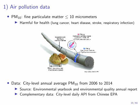
• PM10: fine particulate matter 10 micrometersI Harmful for health (lung cancer, heart disease, stroke, respiratory infection)
4/21/15 10:09 PMParticulate Matter | Air Research | Research Priorities | Research | US EPA
Page 1 of 1http://www.epa.gov/airscience/air-particulate-matter-image.htm
Last updated on May 18, 2012
http://www.epa.gov/airscience/air-particulate-matter-image.htm
Particulate MatterParticulate Matter (PM) Science
• Data: City-level annual average PM10 from 2006 to 2014I Source: Environmental yearbook and environmental quality annual reportI Complementary data: City-level daily API from Chinese EPA
13 / 61
1) Air pollution data
• PM10: fine particulate matter 10 micrometersI Harmful for health (lung cancer, heart disease, stroke, respiratory infection)
4/21/15 10:09 PMParticulate Matter | Air Research | Research Priorities | Research | US EPA
Page 1 of 1http://www.epa.gov/airscience/air-particulate-matter-image.htm
Last updated on May 18, 2012
http://www.epa.gov/airscience/air-particulate-matter-image.htm
Particulate MatterParticulate Matter (PM) Science
• Data: City-level annual average PM10 from 2006 to 2014I Source: Environmental yearbook and environmental quality annual reportI Complementary data: City-level daily API from Chinese EPA
13 / 61
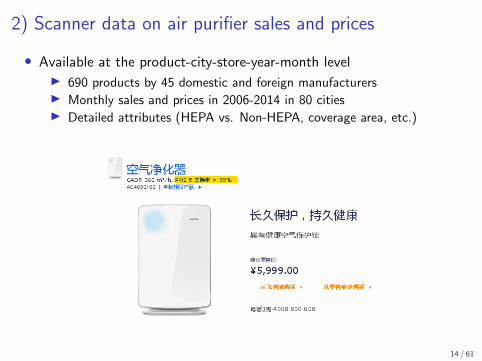
2) Scanner data on air purifier sales and prices
• Available at the product-city-store-year-month levelI 690 products by 45 domestic and foreign manufacturersI Monthly sales and prices in 2006-2014 in 80 citiesI Detailed attributes (HEPA vs. Non-HEPA, coverage area, etc.)
14 / 61

HEPA vs. Non-HEPA air purifiers
• High E�ciency Particulate Arrestance (HEPA):I A necessary attribute for air purifiers to remove PMI It must remove 99.97% of particles � 0.3 micrometer (US DOE)I Ads in Chinese market: it removes > 99% of PM2.5 and PM10
• Non-HEPA filtration systems do not remove PMI It does not remove fine particles such as PM2.5 and PM10
I However, it still provides other benefitsI e.g. Remove Volatile Organic Compounds (VOC), gas and odors
15 / 61

Summary statistics of air purifier dataTable 1: Summary Statistics of Air Purifier Data
Panel A: Air purifier attributes
All purifiers HEPA Non-HEPA Di�erencepurifiers purifiers in means
Price of a purifier ($) 454.52 509.64 369.81 139.84***(383.81) (404.24) (333.45) [52.14]
Humidifing (0 or 1) 0.164 0.177 0.143 0.034(0.370) (0.382) (0.351) [0.070]
Room coverage (square meter) 41.85 44.97 36.50 8.47*(23.65) (24.93) (20.27) [4.42]
Distance to factory or port (in 100 miles) 7.48 7.32 7.72 -0.39(2.87) (2.69) (3.12) [0.45]
Price of a replacement filter ($) 46.38 56.39 34.92 21.47*(52.21) (65.68) (25.91) [10.70]
Frequency of filter replacement (in months) 9.03 10.08 7.92 2.17(5.93) (6.55) (4.97) [1.37]
Panel B: Number of purifier sales/number of households (%)
All purifiers HEPA Non-HEPA HEPA/purifiers purifiers Non-HEPA
(%) (%) (%) (Ratio)
Beijing (North) 17.82 12.10 5.72 2.12Xi‘an (North) 6.20 4.38 1.82 2.41All Northern Cities 4.70 3.16 1.54 2.06Shanghai (South) 8.89 5.08 3.81 1.33Shenzhen (South) 8.35 4.39 3.96 1.11All Southern Cities 3.47 1.94 1.53 1.27
Note: The dataset includes 690 air purifier products from 45 manufactures. 418 products are HEPA purifiersand 272 are non-HEPA purifiers. In Panel A, standard deviations are reported in parentheses, and standarderrors clustered at the manufacture level are reported in brackets. * significant at 10% level; ** significantat 5% level; *** significant at 1% level.
50
1. HEPA purifiers are on average more expensive than non-HEPA purifiers
2. Other attributes are in general quite similar between the two types
16 / 61

3) Census data
• Demographic and economic variables from the confidential census dataI We obtained confidential micro data on demographic variables, which
include a random sample of households in each cityI We also collected economic data (e.g. GDP) at the city-year level
17 / 61

Outline of this talk
• Introduction
• Background and Data
• Demand Model
• Empirical Analysis and Results
• Policy Implications
• Conclusion
• Appendix
18 / 61

Demand Model
• xc : Ambient air pollution in city c
• xjc : A reduction in indoor air pollution given the purchase of purifier j
xjc = xc · ej
I ej : E↵ectiveness in removing PM10
• Conditional indirect utility of consumer i who purchases purifier j
uijc = �ix jc + ↵ipjc + ⌘j + ⇠jc + ✏ijc
I �: marginal utility for a pollution reduction. ↵: disutility for priceI Note: purifiers are durable goods and last for five years on average
19 / 61

1) Standard Logit Demand Approach (�i = � & ↵i = ↵)
• Assume that ✏ijct ⇠ extreme value type I distribution
• The market share for air purifier j in city c is:
sjc =exp(�x jc + ↵pjc + ⌘j + ⇠jc)PJ
k=0 exp(�xkc + ↵pkc + ⌘k + ⇠kc)
I The outside option (j = 0) is not to buy any air purifierI We assume that x0c = 0 (a reduction in indoor air pollution is zero)
• Log market share for j minus log market share for outside option:
lnsjc � lns0c = �x jc + ↵pjc + ⌘j + ⇠jc
20 / 61

1) Standard Logit Demand Approach
• Reductions in indoor pollution (xjc) can be written by:
xjc = xc · HEPAj =
(xc if HEPAj = 1
0 if HEPAj = 0.
• With city fixed e↵ects (�c), the estimating equation becomes:
lnsjc = �xc · HEPAj + ↵pjc + ⌘j + �c + ⇠jc
I � �↵ = Marginal WTP for a reduction in indoor pollution
• Our estimate is likely to be a lower bound of MWTPI Households may take other avoidance methods for indoor air pollution
(e.g. improve building installation) ! We underestimate their MWTP
21 / 61
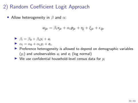
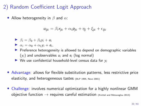
2) Random Coe�cient Logit Approach
• Allow heterogeneity in � and ↵:
uijc = �ixjc + ↵ipjc + ⌘j + ⇠jc + ✏ijc
I �i = �0 + �1yi + ui
I ↵i = ↵0 + ↵1yi + ei ,I Preference heterogeneity is allowed to depend on demographic variables
(yi ) and unobservables ui and ei (log normal)I We use confidential household-level census data for yi
• Advantage: allows for flexible substitution patterns, less restrictive price
elasticity, and heterogeneous tastes (BLP 1995, Nevo 2001)
• Challenge: involves numerical optimization for a highly nonlinear GMM
objective function ! requires careful estimation (Knittel and Metaxoglou 2013)
22 / 61

Note about a potential dynamic decision
• In this paper, we abstract from a consumer’s dynamic decisionI In our setting, exogenous variation in pollution comes from cross-sectionI To exploit this variation, we aggregate our panel data to cross-section
• A new paper in progress: a dynamic discrete choiceI Test if consumers respond to inter-temporal price variationI Investigate how consumers respond to product entries and exits
23 / 61

Outline of this talk
• Introduction
• Background and Data
• Demand Model
• Empirical Analysis and Results
• Policy Implications
• Conclusion
• Appendix
24 / 61

Endogeneity in pollution (x) and price (p)
lnsjc = �xc · HEPAj + ↵pjc + ⌘j + �c + ✏jc
1. Pollution is likely to be correlated with unobserved economic factorsI We exploit spatial RD of the Huai River heating policy
25 / 61

Huai river policy created long-run variation in air pollutionFigure 1: Huai River Boundary and City Locations
Note: The line in the middle of the map shows the Huai River-Qinling boundary.
46
• Government built coal-based centralized heating in the North• Created plausibly exogenous, long-run variation in air pollution
26 / 61

Institutional details of the Huai River heating policy
• In 1958, the Chinese government built centralized heating systemsI Only for the cities north of the Huai River borderlineI Reason: Average January temperature is roughly 0�C along the lineI This line is not used for any other administrative purposes
• Coal-based facilities produce local air pollutionI Heat is generated by local boilers within a residential complexI This create local air pollution for residents in northern cities
27 / 61

1) First stage on PM10
7080
9010
011
012
013
0PM
10
-4 -3.5 -3 -2.5 -2 -1.5 -1 -.5 0 .5 1 1.5 2 2.5 3 3.5 4Distance North to the Huai River (100 miles)
• North of the Huai river ! Higher PM1028 / 61

1) First stage on PM10Table 3: First Stage Estimation for PM10 and Air Purifier Price
(a) First stage estimation for PM10
Dependent variable: PM10 in ug/m3
(1) (2) (3) (4)
North 24.54��� 24.55��� 24.38��� 24.19���
(6.97) (6.98) (8.71) (8.86)
Observations 49 49 49 49R2 0.36 0.36 0.56 0.57Control function for running variable Linear*North Quadratic Linear*North QuadraticDemographic controls Y YLongitude quartile FE Y Y
(b) First stage estimation for air purifier price
Dependent variable: Price ($)
(1) (2) (3) (4)
Distance to factory in 100 miles 18.43��� 18.39��� 12.70�� 12.67��
(4.97) (4.98) (4.94) (4.93)
(Distance to factory in 100 miles)2 -2.32��� -2.33��� -1.49� -1.49�
(0.72) (0.72) (0.77) (0.77)
(Distance to factory in 100 miles)3 0.10��� 0.10��� 0.06 0.06(0.03) (0.03) (0.04) (0.04)
Observations 7,359 7,359 7,359 7,359R2 0.96 0.96 0.96 0.96Control function for running variable Linear*North Quadratic Linear*North QuadraticProduct FE Y Y Y YCity FE Y YLongitude quartile FE*HEPA Y Y Y Y
Predicted e�ect of 500 miles on price 46.46��� 46.30��� 33.22��� 33.16���
(12.07) (12.15) (11.43) (11.42)Predicted e�ect as % of mean price 10.2% 10.2% 7.3% 7.3%
Note: Observations in Panel A are at the city level, and observations in Panel B are at the product-by-citylevel. Demographic controls include population and GDP per capita from City Statistical Yearbook (2006-2014), and average years of schooling and the percentage of population that have completed college fromthe 2005 census microdata. The distance variable in Panel B measures each product’s distances betweenthe manufacturing factory/importing port to markets. We also include the interaction of the linear distancevariable with manufacturer dummy variables to allow a flexible functional form for the relationship betweenprices and distance. * significant at 10% level; ** significant at 5% level; *** significant at 1% level.
52
• Main result: Local linear regression with the bandwidth of 400 miles
• Robust to other choices of bandwidths and functional forms (appendix)
• The amount of PM10 generated by the Huai River Policy = 24.5 ug/m3
29 / 61

Identification assumption behind the RD design
• Assumption: Potential outcomes have to be smooth at the RD cuto↵I As always, this is an untestable assumption (Imbens and Lemieux, 2008)
• We provide two sets of evidence that support this assumption
1. Smoothness of observable variables at the RD cuto↵ (next slide)2. Include longitude quartile FE to control for west-east unobserved factors
30 / 61

Table 2: Summary Statistics of Observables for the North and South of the Huai River
(1) (2) (3) (4)Di�erences RD Estimates
North South in Means (local linear)
Population (1,000,000) 2.398 2.720 -0.323 -0.388(2.266) (3.189) [0.625] [1.411]
Urban population (1,000,000) 1.773 1.974 -0.200 -1.092(1.770) (2.436) [0.480] [1.151]
Years of schooling 9.30 8.64 0.667*** -0.101(0.88) (1.12) [0.227] [0.671]
Fraction illiterate 0.052 0.069 -0.016** 0.003(0.022) (0.033) (0.006) (0.018)
Fraction completed high school 0.338 0.286 0.051** 0.018(0.107) (0.112) [0.025] [0.074]
Fraction completed college 0.052 0.048 0.004 -0.019(0.033) (0.031) [0.007] [0.021]
Per capita household income 527.52 698.10 -170.58** -134.54(USD in 2005) (152.79) (388.20) [67.27] [107.41]
House size (square meter) 75.24 92.04 -16.80*** -12.25(13.32) (17.52) [3.51] [9.34]
Residence built after 1985 0.691 0.718 -0.027 -0.040(0.083) (0.075) [0.018] [0.027]
Fraction building materials include 0.668 0.729 -0.061 0.010reinforced concrete (less insulated) (0.187) (0.147) [0.037] [0.107]
Fraction moved within city 0.074 0.065 0.009 -0.002(0.030) (0.022) [0.006] [0.010]
Fraction occupation involved with 0.218 0.208 0.011 0.032outdoor activities (0.106) (0.099) [0.023] [0.074]
Note: In columns (1)-(2), standard deviations are reported in parentheses. In columns (3)-(4), standarderrors are reported in brackets. * significant at 10% level; ** significant at 5% level; *** significant at 1%level.
51
31 / 61

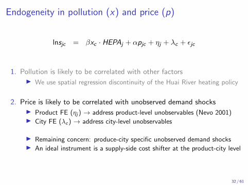
Endogeneity in pollution (x) and price (p)
lnsjc = �xc · HEPAj + ↵pjc + ⌘j + �c + ✏jc
1. Pollution is likely to be correlated with other factorsI We use spatial regression discontinuity of the Huai River heating policy
2. Price is likely to be correlated with unobserved demand shocks
I Product FE (⌘j) ! address product-level unobservables (Nevo 2001)I City FE (�c) ! address city-level unobservables
I Remaining concern: produce-city specific unobserved demand shocksI An ideal instrument is a supply-side cost shifter at the product-city levelI Our idea: the transportation cost from factory/port to market
32 / 61

Endogeneity in pollution (x) and price (p)
lnsjc = �xc · HEPAj + ↵pjc + ⌘j + �c + ✏jc
1. Pollution is likely to be correlated with other factorsI We use spatial regression discontinuity of the Huai River heating policy
2. Price is likely to be correlated with unobserved demand shocksI Product FE (⌘j) ! address product-level unobservables (Nevo 2001)
I City FE (�c) ! address city-level unobservables
I Remaining concern: produce-city specific unobserved demand shocksI An ideal instrument is a supply-side cost shifter at the product-city levelI Our idea: the transportation cost from factory/port to market
32 / 61

Endogeneity in pollution (x) and price (p)
lnsjc = �xc · HEPAj + ↵pjc + ⌘j + �c + ✏jc
1. Pollution is likely to be correlated with other factorsI We use spatial regression discontinuity of the Huai River heating policy
2. Price is likely to be correlated with unobserved demand shocksI Product FE (⌘j) ! address product-level unobservables (Nevo 2001)I City FE (�c) ! address city-level unobservables
I Remaining concern: produce-city specific unobserved demand shocksI An ideal instrument is a supply-side cost shifter at the product-city levelI Our idea: the transportation cost from factory/port to market
32 / 61
Endogeneity in pollution (x) and price (p)
lnsjc = �xc · HEPAj + ↵pjc + ⌘j + �c + ✏jc
1. Pollution is likely to be correlated with other factorsI We use spatial regression discontinuity of the Huai River heating policy
2. Price is likely to be correlated with unobserved demand shocksI Product FE (⌘j) ! address product-level unobservables (Nevo 2001)I City FE (�c) ! address city-level unobservables
I Remaining concern: produce-city specific unobserved demand shocksI An ideal instrument is a supply-side cost shifter at the product-city level
I Our idea: the transportation cost from factory/port to market
32 / 61

Endogeneity in pollution (x) and price (p)
lnsjc = �xc · HEPAj + ↵pjc + ⌘j + �c + ✏jc
1. Pollution is likely to be correlated with other factorsI We use spatial regression discontinuity of the Huai River heating policy
2. Price is likely to be correlated with unobserved demand shocksI Product FE (⌘j) ! address product-level unobservables (Nevo 2001)I City FE (�c) ! address city-level unobservables
I Remaining concern: produce-city specific unobserved demand shocksI An ideal instrument is a supply-side cost shifter at the product-city levelI Our idea: the transportation cost from factory/port to market
32 / 61

2) First stage on price (IV: road distance to factory/port)
• We collected data on each product’s factory/port location• Use GIS to obtain the road distance from factory/port to market
33 / 61

Table 3: First Stage Estimation for PM10 and Air Purifier Price
(a) First stage estimation for PM10
Dependent variable: PM10 in ug/m3
(1) (2) (3) (4)
North 24.54��� 24.55��� 24.38��� 24.19���
(6.97) (6.98) (8.71) (8.86)
Observations 49 49 49 49R2 0.36 0.36 0.56 0.57Control function for running variable Linear*North Quadratic Linear*North QuadraticDemographic controls Y YLongitude quartile FE Y Y
(b) First stage estimation for air purifier price
Dependent variable: Price ($)
(1) (2) (3) (4)
Distance to factory in 100 miles 18.43��� 18.39��� 12.70�� 12.67��
(4.97) (4.98) (4.94) (4.93)
(Distance to factory in 100 miles)2 -2.32��� -2.33��� -1.49� -1.49�
(0.72) (0.72) (0.77) (0.77)
(Distance to factory in 100 miles)3 0.10��� 0.10��� 0.06 0.06(0.03) (0.03) (0.04) (0.04)
Observations 7,359 7,359 7,359 7,359R2 0.96 0.96 0.96 0.96Control function for running variable Linear*North Quadratic Linear*North QuadraticProduct FE Y Y Y YCity FE Y YLongitude quartile FE*HEPA Y Y Y Y
Predicted e�ect of 500 miles on price 46.46��� 46.30��� 33.22��� 33.16���
(12.07) (12.15) (11.43) (11.42)Predicted e�ect as % of mean price 10.2% 10.2% 7.3% 7.3%
Note: Observations in Panel A are at the city level, and observations in Panel B are at the product-by-citylevel. Demographic controls include population and GDP per capita from City Statistical Yearbook (2006-2014), and average years of schooling and the percentage of population that have completed college fromthe 2005 census microdata. The distance variable in Panel B measures each product’s distances betweenthe manufacturing factory/importing port to markets. We also include the interaction of the linear distancevariable with manufacturer dummy variables to allow a flexible functional form for the relationship betweenprices and distance. * significant at 10% level; ** significant at 5% level; *** significant at 1% level.
52
• Longer distance from factory/port to market ! Higher prices34 / 61

010
2030
4050
Cha
nge
in p
rice
pred
icte
d by
dis
tanc
e (U
SD)
0 1 2 3 4 5 6 7 8 9 10Road distance from factory/port to market in 100 miles
• The predicted price-distance relationship35 / 61

An alternative instrument for price as a robustness check
• IO theory predicts that pjc can be a↵ected by its competitor’s costI Consider imperfect competition in di↵erentiated products marketsI A firm sets a higher pjc when its competitors have higher marginal costsI pjc can be a↵ected by the transportation costs of other firms in market c
• IV: Average road distance of the products sold by competing firmsI Appendix Table A.2: the results remain similar to our main results
36 / 61

An alternative instrument for price as a robustness check
• IO theory predicts that pjc can be a↵ected by its competitor’s costI Consider imperfect competition in di↵erentiated products marketsI A firm sets a higher pjc when its competitors have higher marginal costsI pjc can be a↵ected by the transportation costs of other firms in market c
• IV: Average road distance of the products sold by competing firms
I Appendix Table A.2: the results remain similar to our main results
36 / 61
An alternative instrument for price as a robustness check
• IO theory predicts that pjc can be a↵ected by its competitor’s costI Consider imperfect competition in di↵erentiated products marketsI A firm sets a higher pjc when its competitors have higher marginal costsI pjc can be a↵ected by the transportation costs of other firms in market c
• IV: Average road distance of the products sold by competing firmsI Appendix Table A.2: the results remain similar to our main results
36 / 61

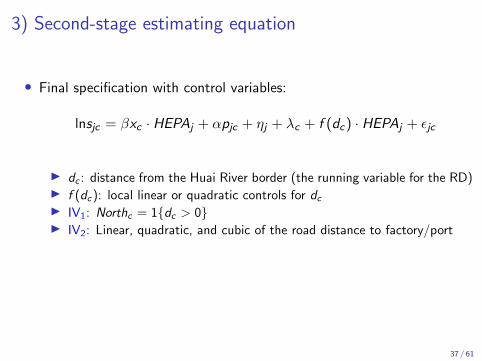
3) Second-stage estimating equation
• Final specification with control variables:
lnsjc = �xc · HEPAj + ↵pjc + ⌘j + �c + f (dc) · HEPAj + ✏jc
I dc : distance from the Huai River border (the running variable for the RD)I f (dc): local linear or quadratic controls for dc
I IV1: Northc = 1{dc > 0}I IV2: Linear, quadratic, and cubic of the road distance to factory/portI Optimal bandwidth is 400 miles from the river (Imbens and Kalyanaraman 2012)
I We report robustness checks with further narrower bandwidthsI Standard errors are clustered at the city level
37 / 61
3) Second-stage estimating equation
• Final specification with control variables:
lnsjc = �xc · HEPAj + ↵pjc + ⌘j + �c + f (dc) · HEPAj + ✏jc
I dc : distance from the Huai River border (the running variable for the RD)I f (dc): local linear or quadratic controls for dcI IV1: Northc = 1{dc > 0}I IV2: Linear, quadratic, and cubic of the road distance to factory/port
I Optimal bandwidth is 400 miles from the river (Imbens and Kalyanaraman 2012)
I We report robustness checks with further narrower bandwidthsI Standard errors are clustered at the city level
37 / 61

3) Second-stage estimating equation
• Final specification with control variables:
lnsjc = �xc · HEPAj + ↵pjc + ⌘j + �c + f (dc) · HEPAj + ✏jc
I dc : distance from the Huai River border (the running variable for the RD)I f (dc): local linear or quadratic controls for dcI IV1: Northc = 1{dc > 0}I IV2: Linear, quadratic, and cubic of the road distance to factory/portI Optimal bandwidth is 400 miles from the river (Imbens and Kalyanaraman 2012)
I We report robustness checks with further narrower bandwidths
I Standard errors are clustered at the city level
37 / 61

3) Second-stage estimating equation
• Final specification with control variables:
lnsjc = �xc · HEPAj + ↵pjc + ⌘j + �c + f (dc) · HEPAj + ✏jc
I dc : distance from the Huai River border (the running variable for the RD)I f (dc): local linear or quadratic controls for dcI IV1: Northc = 1{dc > 0}I IV2: Linear, quadratic, and cubic of the road distance to factory/portI Optimal bandwidth is 400 miles from the river (Imbens and Kalyanaraman 2012)
I We report robustness checks with further narrower bandwidthsI Standard errors are clustered at the city level
37 / 61

3) Second-stage estimation results
Table 4: Standard Logit: Reduced Form and Second Stage Estimation Results
Panel A: Reduced form of the RD design
Dependent variable: ln(market share)
(1) (2)
North*HEPA (⇢) 0.4275��� 0.4216���
(0.0329) (0.0320)
Price (↵) -0.0052��� -0.0052���
(0.0001) (0.0001)
Observations 7,359 7,359First-stage F-Stat 870.29 1115.94Control function for running variable Linear*North Quadratic
Panel B: Second stage of the RD design
Dependent variable: ln(market share)
(1) (2)
PM10*HEPA (�) 0.0299��� 0.0302���
(0.0030) (0.0032)
Price (↵) -0.0048��� -0.0048���
(0.0001) (0.0001)
Observations 7,359 7,359First-stage F-Stat 285.16 292.01Control function for running variable Linear*North Quadratic
MWTP for 5 years (-�/↵) 6.2077��� 6.3100���
(0.6649) (0.7130)MWTP per year 1.2415��� 1.2620���
(0.1330) (0.1426)
Note: Panel A shows results for the reduced-form estimation in equation (8). All regressions include productfixed e�ects, city fixed e�ects, and longitude quartile fixed e�ects interacted with HEPA. Price is instrumentedwith the distance variables discussed in the text. Panel B shows results for the second-stage estimationin equation (9). PM10*HEPA and Price are instrumented with North*HEPA and the distance variablesdiscussed in the text. We use the two-step linear GMM estimation with the optimal weight matrix. Standarderrors are clustered at the city level. * significant at 10% level; ** significant at 5% level; *** significant at1% level. We also report the Kleibergen-Paap rk Wald F-statistic. The Stock-Yogo weak identification testcritical value for one endogenous variable (10% maximal IV size) is 16.38, and for two endogenous variables(10% maximal IV size) it is 7.03.
53
• MWTP = $1.24 per 1 ug/m3 reduction in PM10 per year
• Results are robust to the choice of bandwidths (next slide)
38 / 61

Table 5: Robustness Checks
Panel A: Control function for the running variable: Linear*North
Dependent variable: ln(market share)
(1) 250 miles (2) 300 miles (3) 350 miles (4) 400 miles
PM10*HEPA (�) 0.0296��� 0.0322��� 0.0268��� 0.0299���
(0.0029) (0.0047) (0.0010) (0.0030)
Price (↵) -0.0036��� -0.0038��� -0.0042��� -0.0048���
(0.0002) (0.0002) (0.0001) (0.0001)
Observations 5,619 5,878 7,107 7,359First-stage F-Stat 1921.77 526.20 1348.93 285.16
MWTP for 5 years (-�/↵) 8.2840��� 8.4562��� 6.3748��� 6.2077���
(1.0665) (1.4798) (0.2764) (0.6649)MWTP per year 1.6568��� 1.6912��� 1.2750��� 1.2415���
(0.2133) (0.2960) (0.0553) (0.1330)
Panel B: Control function for the running variable: Quadratic
Dependent variable: ln(market share)
(1) 250 miles (2) 300 miles (3) 350 miles (4) 400 miles
PM10*HEPA (�) 0.0298��� 0.0327��� 0.0265��� 0.0302���
(0.0028) (0.0046) (0.0010) (0.0032)
Price (↵) -0.0035��� -0.0037��� -0.0042��� -0.0048���
(0.0002) (0.0002) (0.0001) (0.0001)
Observations 5,619 5,878 7,107 7,359First-stage F-Stat 2122.08 467.03 1399.44 292.01
MWTP for 5 years (-�/↵) 8.4464��� 8.7436��� 6.3470��� 6.3100���
(1.0758) (1.5087) (0.3034) (0.7130)MWTP per year 1.6893��� 1.7487��� 1.2694��� 1.2620���
(0.2152) (0.3017) (0.0607) (0.1426)
Note: This table shows results for the second-stage estimation in equation (9) with alternative choices ofbandwidth and control functions for the running variable. All regressions include product fixed e�ects, cityfixed e�ects, and longitude quartile fixed e�ects interacted with HEPA. See notes in Table 4. Standarderrors are clustered at the city level. * significant at 10% level; ** significant at 5% level; *** significant at1% level. We also report the Kleibergen-Paap rk Wald F-statistic. The Stock-Yogo weak identification testcritical value for two endogenous variables (10% maximal IV size) is 7.03.
54
39 / 61

4) What variation in the data identifies �?
• Recall that the second-stage of the RD design is:
lnsjc = �xc · HEPAj + ↵pjc + ⌘j + �c + f (dc) · HEPAj + ✏jc
• To visualize what variation in the data is identifying �, it is useful to
see the reduced-form relationship of the RD design
• Reduced-form relationship of the RD design is:
lnsjc = ⇢Northc · HEPAj + ↵pjc + ⌘j + �c + f (dc) · HEPAj + ✏jc
40 / 61

Reduced-form of the RD design
lnsjc = ⇢Northc · HEPAj + ↵pjc + ⌘j + �c + f (dc) · HEPAj + ✏jcTable 4: Standard Logit: Reduced Form and Second Stage Estimation Results
Panel A: Reduced form of the RD design
Dependent variable: ln(market share)
(1) (2)
North*HEPA (⇢) 0.4275��� 0.4216���
(0.0329) (0.0320)
Price (↵) -0.0052��� -0.0052���
(0.0001) (0.0001)
Observations 7,359 7,359First-stage F-Stat 870.29 1115.94Control function for running variable Linear*North Quadratic
Panel B: Second stage of the RD design
Dependent variable: ln(market share)
(1) (2)
PM10*HEPA (�) 0.0299��� 0.0302���
(0.0030) (0.0032)
Price (↵) -0.0048��� -0.0048���
(0.0001) (0.0001)
Observations 7,359 7,359First-stage F-Stat 285.16 292.01Control function for running variable Linear*North Quadratic
MWTP for 5 years (-�/↵) 6.2077��� 6.3100���
(0.6649) (0.7130)MWTP per year 1.2415��� 1.2620���
(0.1330) (0.1426)
Note: Panel A shows results for the reduced-form estimation in equation (8). All regressions include productfixed e�ects, city fixed e�ects, and longitude quartile fixed e�ects interacted with HEPA. Price is instrumentedwith the distance variables discussed in the text. Panel B shows results for the second-stage estimationin equation (9). PM10*HEPA and Price are instrumented with North*HEPA and the distance variablesdiscussed in the text. We use the two-step linear GMM estimation with the optimal weight matrix. Standarderrors are clustered at the city level. * significant at 10% level; ** significant at 5% level; *** significant at1% level. We also report the Kleibergen-Paap rk Wald F-statistic. The Stock-Yogo weak identification testcritical value for one endogenous variable (10% maximal IV size) is 16.38, and for two endogenous variables(10% maximal IV size) it is 7.03.
53
41 / 61
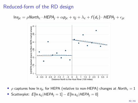
Reduced-form of the RD design
lnsjc = ⇢Northc · HEPAj + ↵pjc + ⌘j + �c + f (dc) · HEPAj + ✏jc
-1-.7
5-.5
-.25
0.2
5.5
ln(H
EPA
mar
ket s
hare
)-ln(
Non
-HEP
A m
arke
t sha
re)
-4 -3.5 -3 -2.5 -2 -1.5 -1 -.5 0 .5 1 1.5 2 2.5 3 3.5 4Distance North to the Huai River (100 miles)
• ⇢ captures how ln sjc for HEPA (relative to non-HEPA) changes at Northc = 1
• Scatterplot: E [ln scj |HEPAj = 1] � E [ln scj |HEPAj = 0]
42 / 61
5) Random-coe�cient logit approach
• Allow heterogeneity in � and ↵
uijc = �ixjc + ↵ipjc + ⌘j + ✏jc + ✏ijc
I �i = �0 + �1yi + ui
I ↵i = ↵0 + ↵1yi + ei ,I Preference heterogeneity is allowed to depend on demographic variables
(yi ) and unobservables ui and ei
I We use micro data on household-level income from census for yi
• Nonlinear numerical optimization requires careful investigation
1. Test several nonlinear search algorithms2. Test 100 sets of random starting values for each search algorithm3. Use conservative tolerance levels for fixed-point iterations
43 / 61

Box plot: Objective function values from 100 staring points
350 400 450 500 550 600Objective Function Value
Solvopt
Simplex
Quasi-Newton 2
Quasi-Newton 1
GPS
Conjugate gradient
• Implications
1. Testing many staring values is important for nonlinear optimization2. In our case, all search algorithms (except for conjugate gradient) reached
the same minimum for more than 90% of the 100 sets of starting values44 / 61

Random-coe�cient logit resultsTable 7: Random-Coe�cient Logit Estimation Results
Dependent variable: ln(market share)
(1) (2)
PM10 · HEPA
Mean coe�cient (�0) 0.0459��� 0.0498���
(0.0084) (0.0092)
Interaction household income (�1) 0.0924��� 0.0891���
(0.0224) (0.0253)
Standard deviation (��) 0.0323��� 0.0570���
(0.0117) (0.0119)
Price
Mean coe�cient (↵0) -0.0069��� -0.0071���
(0.0007) (0.0007)
Interaction with household income (↵1) 0.0028�� 0.0028��
(0.0011) (0.0011)
Standard deviation (��) 0.0006 0.0005(0.0007) (0.0007)
Observations 7,359 7,359Control function for running variable Linear*North QuadraticGMM objective function value 375.05 378.93MWTP per year: 5th percentile 0.38 0.07MWTP per year: 10th percentile 0.49 0.20MWTP per year: 25th percentile 0.75 0.53MWTP per year: 50th percentile 1.19 1.10MWTP per year: mean 1.34 1.41MWTP per year: 75th percentile 1.90 2.04MWTP per year: 90th percentile 2.92 3.45MWTP per year: 95th percentile 3.86 4.69
Note: This table shows the results of the random-coe�cient logit estimation in equation (6). All regressionsinclude product fixed e�ects, city fixed e�ects, and longitude quartile fixed e�ects interacted with HEPA.Column 1 uses a linear control for the running variable interacted with the North dummy variable, andcolumn 2 uses a quadratic control for the running variable. Asymptotically robust standard errors are givenin parentheses, which are corrected for the error due to the simulation process by taking account that thesimulation draws are the same for all of the observations in a market. The household-level income data(in 2005 USD) come from the 2005 Chinese census. The distribution of the marginal willingness to pay for
clean air is obtained by mwtpi = �(�̂0 + �̂1yi + ui)/(↵̂0 + ↵̂1yi + ei) using the estimated coe�cients,household-level income, and random draws from standard normal distributions.
56
Table 7: Heterogeneity in WTP for Clean Air: Random-Coe�cient Logit Estimation Results
Dependent variable: ln(market share)
(1) (2)
PM10 · HEPA
Mean coe�cient (�0) 0.0459��� 0.0498���
(0.0084) (0.0092)
Interaction household income (�1) 0.0924��� 0.0891���
(0.0224) (0.0253)
Standard deviation (��) 0.0056��� 0.0102���
(0.0020) (0.0021)
Price
Mean coe�cient (↵0) -0.0069��� -0.0071���
(0.0007) (0.0007)
Interaction with household income (↵1) 0.0028�� 0.0028��
(0.0011) (0.0011)
Standard deviation (��) 0.0026 0.0024(0.0030) (0.0030)
Observations 7,359 7,359Control function for running variable Linear*North QuadraticGMM objective function value 375.05 378.93MWTP per year: 5th percentile 0.38 0.07MWTP per year: 10th percentile 0.49 0.20MWTP per year: 25th percentile 0.75 0.53MWTP per year: 50th percentile 1.19 1.10MWTP per year: mean 1.34 1.41MWTP per year: 75th percentile 1.90 2.04MWTP per year: 90th percentile 2.92 3.45MWTP per year: 95th percentile 3.86 4.69
Notes: This table shows the results of the random-coe�cient logit estimation in equation (6). All regressions includeproduct fixed e�ects, city fixed e�ects, and longitude quartile fixed e�ects interacted with HEPA. Column 1 uses a linearcontrol for the running variable interacted with the North dummy variable, and column 2 uses a quadratic control forthe running variable. Asymptotically robust standard errors are given in parentheses, which are corrected for the errordue to the simulation process by taking account that the simulation draws are the same for all of the observations in amarket.
44
Table 7: Random-Coe�cient Logit Estimation Results
Dependent variable: ln(market share)
(1) (2)
PM10 · HEPA
Mean coe�cient (�0) 0.0459��� 0.0498���
(0.0084) (0.0092)
Interaction household income (�1) 0.0924��� 0.0891���
(0.0224) (0.0253)
Standard deviation (��) 0.0323��� 0.0570���
(0.0117) (0.0119)
Price
Mean coe�cient (↵0) -0.0069��� -0.0071���
(0.0007) (0.0007)
Interaction with household income (↵1) 0.0028�� 0.0028��
(0.0011) (0.0011)
Standard deviation (��) 0.0006 0.0005(0.0007) (0.0007)
Observations 7,359 7,359Control function for running variable Linear*North QuadraticGMM objective function value 375.05 378.93MWTP per year: 5th percentile 0.38 0.07MWTP per year: 10th percentile 0.49 0.20MWTP per year: 25th percentile 0.75 0.53MWTP per year: 50th percentile 1.19 1.10MWTP per year: mean 1.34 1.41MWTP per year: 75th percentile 1.90 2.04MWTP per year: 90th percentile 2.92 3.45MWTP per year: 95th percentile 3.86 4.69
Note: This table shows the results of the random-coe�cient logit estimation in equation (6). All regressionsinclude product fixed e�ects, city fixed e�ects, and longitude quartile fixed e�ects interacted with HEPA.Column 1 uses a linear control for the running variable interacted with the North dummy variable, andcolumn 2 uses a quadratic control for the running variable. Asymptotically robust standard errors are givenin parentheses, which are corrected for the error due to the simulation process by taking account that thesimulation draws are the same for all of the observations in a market. The household-level income data(in 2005 USD) come from the 2005 Chinese census. The distribution of the marginal willingness to pay for
clean air is obtained by mwtpi = �(�̂0 + �̂1yi + ui)/(↵̂0 + ↵̂1yi + ei) using the estimated coe�cients,household-level income, and random draws from standard normal distributions.
56
• Higher income ! Value clean air more (�1 > 0) & less price-elastic (↵1 > 0)
45 / 61

The relationship between MWTP and household income
0
1
2
3
4
5
6
7
8M
argi
nal W
TP p
er y
ear (
$/PM
10)
0 1000 2000 3000 4000 5000 6000 7000 8000 9000 10000Annual household income (USD)
Marginal WTP per year 95% Confidence Interval
• Estimated marginal WTP for clean air is increasing in household income
46 / 61

Heterogeneity in MWTP for clean air
0
.01
.02
.03
.04
.05
.06
.07
.08
.09
.1
.11
.12
Frac
tion
of h
ouse
hold
s
0 2 4 6 8 10Marginal willingness to pay for clean air per year ($/PM10)
• Substantial heterogeneity in MWTP
• Mean ($1.34) is not largely di↵erent from the standard logit result ($1.24)
47 / 61

7) Does MWTP for clean air depend on information?
• Limited information may attenuate WTP for environmental qualityI Especially important in developing countries (Greenstone and Jack, 2013)
I However, it is generally di�cult to test this with non-experimental data
• We use widespread media coverage on air pollution after January 2013I On January 12th 2013, the US Embassy in Beijing posted air quality
index (AQI) of 755, beyond the scale’s maximum 500I New York Times and other foreign medias started extensive coverageI Resulted in widespread media coverage in Chinese newspapers
48 / 61

7) Does MWTP for clean air depend on information?
• Limited information may attenuate WTP for environmental qualityI Especially important in developing countries (Greenstone and Jack, 2013)
I However, it is generally di�cult to test this with non-experimental data
• We use widespread media coverage on air pollution after January 2013
I On January 12th 2013, the US Embassy in Beijing posted air qualityindex (AQI) of 755, beyond the scale’s maximum 500
I New York Times and other foreign medias started extensive coverageI Resulted in widespread media coverage in Chinese newspapers
48 / 61

7) Does MWTP for clean air depend on information?
• Limited information may attenuate WTP for environmental qualityI Especially important in developing countries (Greenstone and Jack, 2013)
I However, it is generally di�cult to test this with non-experimental data
• We use widespread media coverage on air pollution after January 2013I On January 12th 2013, the US Embassy in Beijing posted air quality
index (AQI) of 755, beyond the scale’s maximum 500
I New York Times and other foreign medias started extensive coverageI Resulted in widespread media coverage in Chinese newspapers
48 / 61

7) Does MWTP for clean air depend on information?
• Limited information may attenuate WTP for environmental qualityI Especially important in developing countries (Greenstone and Jack, 2013)
I However, it is generally di�cult to test this with non-experimental data
• We use widespread media coverage on air pollution after January 2013I On January 12th 2013, the US Embassy in Beijing posted air quality
index (AQI) of 755, beyond the scale’s maximum 500I New York Times and other foreign medias started extensive coverageI Resulted in widespread media coverage in Chinese newspapers
48 / 61

Widespread media coverage has started in January, 2013Figure A.4: Chinese newspaper headlines mentioning air pollution and smog
020
040
060
080
010
0012
0014
0016
00m
entio
ns o
f air
pollu
tion
in h
eadl
ines
2006 2007 2008 2009 2010 2011 2012 2013 2014year
Air pollution SmogNote: Each dot represents the annual number of newspaper headlines mentioning “air pollution” (includingair pollution and ambient air pollution in Chinese) from all 631 newspapers in China. Each triangle representsthe annual number of headlines mentioning “smog”. The data are from the China Core Newspapers Full-textDatabase that collects all newspapers published in China.
61
• Annual number of newspaper headlines from all 631 newspapers in China• We test if the preference for clean air (�) changed in response to this event
49 / 61

We find that MWTP became higher after 2013Table 6: Before and After the Expansion of Media Coverage on Pollution in 2013
Dependent variable: ln(market share)
(1) (2) (3)
PM10*HEPA 0.0192��� 0.0174��� 0.0193���
(0.0018) (0.0027) (0.0025)
PM10*HEPA*Post-2013 0.0329��� 0.0307��� 0.0280���
(0.0076) (0.0079) (0.0090)
Price -0.0072��� -0.0072��� -0.0064���
(0.0001) (0.0002) (0.0002)
Observations 10,780 10,780 10,780First-stage F-Stat 113.39 112.01 189.15Control function for running variable Linear*North Linear*North Linear*NorthProduct FE*Post-2013 Y Y YCity FE*Post-2013 Y Y YLongitude quartile FE*HEPA*Post-2013 Y Y YSalary*HEPA Y YSalary*Price Y
MWTP per year before 2013 0.5313��� 0.4867��� 0.6001���
(0.0595) (0.0874) (0.0918)
MWTP per year after 2013 1.4438��� 1.3458��� 1.4707���
(0.1475) (0.1376) (0.2009)
Di�erence in MWTP per year 0.9124��� 0.8591��� 0.8706���
(0.1961) (0.2040) (0.2647)
Note: This table shows results for the second-stage estimation in equation (9) but allows the preference forair quality (�) to be di�erent before and after 2013. Observations are at the product-city-pre(post) 2013level. Standard errors are clustered at the city level. * significant at 10% level; ** significant at 5% level;*** significant at 1% level. We also report the Kleibergen-Paap rk Wald F-statistic. The Stock-Yogo weakidentification test critical value for one endogenous variable (10% maximal IV size) is 16.38, and for twoendogenous variables (10% maximal IV size) it is 7.03.
55
Table 6: Before and After the Expansion of Media Coverage on Pollution in 2013
Dependent variable: ln(market share)
(1) (2) (3)
PM10*HEPA 0.0192��� 0.0174��� 0.0193���
(0.0018) (0.0027) (0.0025)
PM10*HEPA*Post-2013 0.0329��� 0.0307��� 0.0280���
(0.0076) (0.0079) (0.0090)
Price -0.0072��� -0.0072��� -0.0064���
(0.0001) (0.0002) (0.0002)
Observations 10,780 10,780 10,780First-stage F-Stat 113.39 112.01 189.15Control function for running variable Linear*North Linear*North Linear*NorthProduct FE*Post-2013 Y Y YCity FE*Post-2013 Y Y YLongitude quartile FE*HEPA*Post-2013 Y Y YSalary*HEPA Y YSalary*Price Y
MWTP per year before 2013 0.5313��� 0.4867��� 0.6001���
(0.0595) (0.0874) (0.0918)
MWTP per year after 2013 1.4438��� 1.3458��� 1.4707���
(0.1475) (0.1376) (0.2009)
Di�erence in MWTP per year 0.9124��� 0.8591��� 0.8706���
(0.1961) (0.2040) (0.2647)
Note: This table shows results for the second-stage estimation in equation (9) but allows the preference forair quality (�) to be di�erent before and after 2013. Observations are at the product-city-pre(post) 2013level. Standard errors are clustered at the city level. * significant at 10% level; ** significant at 5% level;*** significant at 1% level. We also report the Kleibergen-Paap rk Wald F-statistic. The Stock-Yogo weakidentification test critical value for one endogenous variable (10% maximal IV size) is 16.38, and for twoendogenous variables (10% maximal IV size) it is 7.03.
55
50 / 61
Outline of this talk
• Introduction
• Background and Data
• Demand Model
• Empirical Analysis and Results
• Policy Implications
• Conclusion
• Appendix
51 / 61

Policy implications
• Policy debate on the tradeo↵ between growth and environmentI Chinese Premier Li Keqiang declared “War Against Pollution” in 2014I A key question is whether such policies enhance social welfare
• Example: A pilot reform for the Huai river policyI Recently implemented by the Chinese government and the World BankI Make the heating system more e�cient and less polluted in pilot cities
52 / 61

Make the heating system more e�cient and less polluted
Source: Chianews.com
• The cost-e↵ectiveness of this policy is still under debate
• How can we use our WTP estimate for this policy discussion?
53 / 61

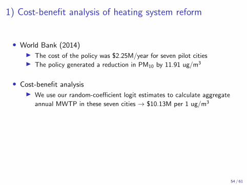
1) Cost-benefit analysis of heating system reform
• World Bank (2014)I The cost of the policy was $2.25M/year for seven pilot citiesI The policy generated a reduction in PM10 by 11.91 ug/m3
• Cost-benefit analysisI We use our random-coe�cient logit estimates to calculate aggregate
annual MWTP in these seven cities ! $10.13M per 1 ug/m3
I This implies that WTP for the 11.91 ug/m3 reduction is $120.63MI Benefit-cost ratio = 53.6 (= 120.63/2.25)
• Benefit-cost ratio > 0, even with our lower bound MWTP estimate
54 / 61
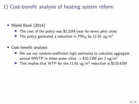
1) Cost-benefit analysis of heating system reform
• World Bank (2014)I The cost of the policy was $2.25M/year for seven pilot citiesI The policy generated a reduction in PM10 by 11.91 ug/m3
• Cost-benefit analysisI We use our random-coe�cient logit estimates to calculate aggregate
annual MWTP in these seven cities ! $10.13M per 1 ug/m3
I This implies that WTP for the 11.91 ug/m3 reduction is $120.63M
I Benefit-cost ratio = 53.6 (= 120.63/2.25)
• Benefit-cost ratio > 0, even with our lower bound MWTP estimate
54 / 61

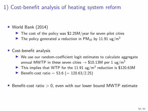
1) Cost-benefit analysis of heating system reform
• World Bank (2014)I The cost of the policy was $2.25M/year for seven pilot citiesI The policy generated a reduction in PM10 by 11.91 ug/m3
• Cost-benefit analysisI We use our random-coe�cient logit estimates to calculate aggregate
annual MWTP in these seven cities ! $10.13M per 1 ug/m3
I This implies that WTP for the 11.91 ug/m3 reduction is $120.63MI Benefit-cost ratio = 53.6 (= 120.63/2.25)
• Benefit-cost ratio > 0, even with our lower bound MWTP estimate
54 / 61
1) Cost-benefit analysis of heating system reform
• World Bank (2014)I The cost of the policy was $2.25M/year for seven pilot citiesI The policy generated a reduction in PM10 by 11.91 ug/m3
• Cost-benefit analysisI We use our random-coe�cient logit estimates to calculate aggregate
annual MWTP in these seven cities ! $10.13M per 1 ug/m3
I This implies that WTP for the 11.91 ug/m3 reduction is $120.63MI Benefit-cost ratio = 53.6 (= 120.63/2.25)
• Benefit-cost ratio > 0, even with our lower bound MWTP estimate
54 / 61

2) Does the WTP justify replacing coal power plants?
• We provide a similar benefit-cost calculation for this questionI Result: Our WTP estimate by itself is unlikely to justify this proposal
• Reason: Coal is substantially cheaper than other options in ChinaI Natural gas in China is not as inexpensive as the one currently in the USI Renewables are still substantially more expensive than coal in China
55 / 61

Outline of this talk
• Introduction
• Background and Data
• Demand Model
• Empirical Analysis and Results
• Policy Implications
• Conclusion
• Appendix
56 / 61

Summary
1. Develop a framework to estimate WTP for environmental quality frommarket transaction data on di↵erentiated products
2. Provide among the first revealed preference estimates of WTP for cleanair in developing countriesI MWTP (mean) = $1.34 per 1 ug/m3 reduction in PM10 per yearI Substantial heterogeneity in MWTP among householdsI Income and information are key determinants of the heterogeneity
3. O↵er policy implications for environmental policies in ChinaI Heating system reform is likely to be a welfare-enhancing policyI Coal power replacement is unlikely to be justified by our WTP estimate
57 / 61