wider working paper 2018/9 · pdf filejel classification: i12, i20, o15 . acknowledgements:...

WIDER Working Paper 2018/9

Formal education, malaria preventive behaviour, and children’s malarial status in Tanzania

Ninja Ritter Klejnstrup1 and Joel Silas Lincoln2

January 2018

1 University of Copenhagen, Denmark; corresponding author: [email protected]; 2 University of Dar es Salaam, Tanzania.

This study has been prepared within the context of the UNU-WIDER 2014–18 work programme.

Copyright © UNU-WIDER 2018

Information and requests: [email protected]

ISSN 1798-7237 ISBN 978-92-9256-451-3

Typescript prepared by Ayesha Chari.

The United Nations University World Institute for Development Economics Research provides economic analysis and policy advice with the aim of promoting sustainable and equitable development. The Institute began operations in 1985 in Helsinki, Finland, as the first research and training centre of the United Nations University. Today it is a unique blend of think tank, research institute, and UN agency—providing a range of services from policy advice to governments as well as freely available original research.

The Institute is funded through income from an endowment fund with additional contributions to its work programme from Denmark, Finland, Sweden, and the United Kingdom.

Katajanokanlaituri 6 B, 00160 Helsinki, Finland

The views expressed in this paper are those of the author(s), and do not necessarily reflect the views of the Institute or the United Nations University, nor the programme/project donors.

Abstract: In this study, we assess formal education as a causal determinant of women’s malaria preventive behaviour, as well as children’s risk of malaria infection. For identification, we rely on exogenous variation in educational attainment generated by educational reforms during the 1970s. We use data from a total of four rounds of either Demographic and Health Surveys or Malaria Indicator Surveys, which allows us to explore variation in relationships over time. In the earliest survey rounds (2004–05 and 2007–08), our results indicate that each additional year of schooling increased women’s probability of using malaria prophylaxis during pregnancy by between 3.7 and 14.5 percentage points, and their children’s probability of sleeping under an insecticide-treated bed net (ITN) by between 1.8 and 3.0 percentage points. Results for both women’s use of ITN and children’s malaria status are inconclusive across all survey rounds. We argue that differences in magnitude and strength of evidence of causality between effect estimates for women’s use of malaria prophylaxis and women’s and children’s use of ITN is likely due to differences in the mechanisms linking these outcomes to education, with the latter being mediated by income to a higher degree than the former.

Keywords: health behaviour, malaria, school reform, Tanzania JEL classification: I12, I20, O15

Acknowledgements: This research is part of the Growth and Development Research Project (GDRP) funded by DANIDA 2016–18. The GDRP is a collaborative research project between the United Nations University World Institute for Development Economics Research (UNU-WIDER), the Development Economics Research Group at University of Copenhagen in Denmark, and the Department of Economics at the University of Dar es Salaam in Tanzania. We acknowledge the financial support from DANIDA under the GDRP and UNU-WIDER for general collaboration.

mailto:[email protected]

1

1 Introduction

Gaining an understanding of which factors influence health behaviour and health outcomes is a central topic within health economics. This is not least because knowledge of the determinants of health is a prerequisite for effective design and targeting of health interventions. One candidate determinant that receives much attention is education. Thus, a large body of literature suggests that formal schooling is the most important correlate of good health, regardless of the health measure considered (Grossman 2004). Meanwhile, it is a well-known truism that correlation does not necessarily imply causation. As such, correlations between education and health could be wholly or partially due to the correlation of both with third factors, such as preferences or contextual factors, just as it may be that it is in fact health that determines educational outcomes. Recent studies that have relied on the introduction of compulsory schooling laws in the United States and various European countries to study the causal relationship between education and health have arrived at mixed conclusions (Lleras-Muney 2005; Clark and Roayer 2013; Meghir et al. 2013; Gathmann et al. 2015). Hence, unsurprisingly, the literature suggests that the nature of the relationship between education and health or health behaviour varies across both context and the aspects of health considered.

In this paper, we examine education as a causal determinant of health, in the context of malaria and malaria preventive behaviour in Tanzania. Despite large reductions in prevalence over the last decade, malaria continues to be a major public health challenge in several regions of the country. In 2009–10, malaria-related health expenditures accounted for 19 per cent of total health expenditures in the country (Ministry of Health and Social Welfare 2012). In 2012, malaria remained the leading cause of outpatient department visits (accounting for 33 per cent of all visits for children aged below 5 years and 30 per cent of visits for everyone else), the leading cause of hospital admissions (accounting for 40 and 30 per cent of all admissions, respectively), and the leading cause of death in hospitals (accounting for 30 and 22 per cent of all deaths, respectively) (Ministry of Health and Social Welfare 2013).

In spite of this, and the importance of understanding determinants for effective policy design, the nature of the relationship between education and malaria preventive behaviour has received little attention in Tanzania (and, to our knowledge, elsewhere). A series of relatively small, localized studies have estimated the bivariate association between formal education and malaria knowledge and/or preventive behaviour such as use of bed nets (Nganda et al. 2004; Mazigo et al. 2010; Ambrose et al. 2011; Mathania et al. 2016). These studies have clearly not been able to establish causality, and they have generally differed in their conclusions. Thus, while correct knowledge of transmission is consistently found to correlate with formal education, the few results for malaria preventive behaviour are mixed. In Geita district in north-western Tanzania, Mazigo et al. (2010) find that education does correlate significantly with use of bed nets, whereas Ambrose et al. (2011) find that it does not among pregnant women seeking antenatal care at Iringa Regional Hospital. In Tanga region, Anders et al. (2008) find no significant relationship between education and uptake of intermittent preventive treatment for malaria during pregnancy.

To our knowledge, the most rigorous association of the relationship between formal education, malaria preventive behaviour, and malarial outcomes to date is noted in the study by Njau et al. (2014) who explore the correlates of maternal education and childhood malaria infections across three African countries, of which Tanzania is one. They distinguish between four sets of covariates, which they argue proxy for distinct causal pathways: child health knowledge, economic empowerment, family formation patterns, and social networking. Starting with a baseline specification with a limited set of demographic control variables and cluster fixed effects, they

2

incrementally add these sets of covariates and find that each addition reduces the point estimate on maternal education from the baseline specification. Based on this and a Blinder–Oaxaca decomposition of the gap in malaria prevalence between children of educated and uneducated mothers, they conclude that children’s malaria status does correlate significantly with maternal education, and that health knowledge, economic empowerment, and social networks are important paths through which maternal education influences childhood infection. Meanwhile, as the authors themselves note, their study design does not enable them to explore causality either. As such, they are essentially unable to distinguish spurious correlation or reverse causality from an actual causal pathway running from education through knowledge, empowerment, and networks to health.

We take on the challenge of causal identification, relying on exogenous variation in educational attainment across birth cohorts generated by Tanzanian educational reforms in the 1970s. We are inspired in design by a number of recent studies that have relied on educational reforms to examine causal links between education and HIV or HIV-related behaviour in Zimbabwe (Aguero and Bharadwaj 2014), Botswana (De Neve et al. 2015), and Malawi and Uganda (Behrman 2015). In these countries, educational reforms gave rise to a discontinuity in the relationship between birth year and educational attainment. This enabled the authors to explore causality based on regression discontinuity designs. In the Tanzanian case, however, the series of educational reforms that were implemented during the 1970s gave rise to a kinked relationship. Therefore, we implement our analysis using the relatively novel regression kink (RK) design.

2 Education reforms in Tanzania during the 1970s

Mainland Tanzania became independent of colonial rule in 1961 and united with Zanzibar to form the United Republic of Tanzania in 1964. Prior to independence, access to education had been very limited: by one estimate, in 1947 less than 10 per cent of the school-aged population was enrolled in primary school, and less than 1 per cent in secondary school (Cameron and Dodd 1970, cited in Al-Samarrai and Peasgood 1998). Meanwhile, the first government of the independent republic, headed by Julius Nyerere, viewed education of the people as a central means to national development and a stated goal of self-reliance, and immediately pursued policies to expand access (Mushi 2009). Whereas the initial focus was on secondary and adult education, motivated in part by a need for an immediate skills upgrade of the work force, expansion of access to primary school education played a central role in the 1970s. As early as 1968, a barrier to progression from form IV to form V, in the shape of an entry exam, was removed, and in 1971 primary school fees were formally abolished. Further, while Tanzania’s Second Five-Year Development Plan (1969–74) had stipulated a goal of universal primary education to be achieved by 1989, in 1974 the target year was moved forward to 1977 in what became known as the Musoma Resolution. In 1978, the passing of the National Act No. 25 made primary school attendance compulsory for all children between the ages of 7 and 13 years (Mushi 2009).

Primary school enrolment figures responded immediately to the new educational policies. Figure 1 presents trends in primary school enrolment numbers and gross enrolment ratio over the period 1970–95. Enrolment followed a positive trend from 1970, but there was a clear jump in enrolment in form I between 1974 and 1975, following the passing of the Musoma Resolution. Those who entered primary school in 1975 would have been in form VII in 1981, and in accordance, a jump in enrolment in form VII is found between 1980 and 1981. A second, large jump in enrolment in form I occurred between 1977 and 1978, when primary school became compulsory. Meanwhile, the dropout rate for the cohort that entered school in 1978, implied by the enrolment figures, is striking. Thus, only 70 per cent of those who entered form I in 1978 had progressed to form VII in 1984. The figure also illustrates that following the jump in 1978, enrolment returned to a level

3

just below that of 1977, and subsequently remained relatively stable throughout the 1980s. Together with growth in the size of the primary school-aged population, this implied a decrease in the gross enrolment ratio throughout the 1980s. This development coincided with a general economic decline in the 1980s, and an accompanying deterioration of educational infrastructure (Mushi 2009).

Figure 1: Enrolment in primary education by grade/form and gross enrolment ratio, 1970–95

Source: Based on data from the UNESCO Institute for Statistics (n.d.).

Overall, the pattern of enrolment and the history of educational policies indicate that the expected years of schooling changed markedly across cohorts of children who went to school during the 1970s as a result of policy changes, and hence independently of individual and household characteristics. However, exactly which cohorts were affected to what degree by these policy developments is less clear because (i) a large number of over-age children were enrolled in form I during the period; and (ii) children of different ages are likely to have dropped out at different rates. Thus, children born in 1968 constitute the first cohort to have been exposed to the 1974–75 reform from the year they were intended to enter primary school (at 7 years of age), and children born in 1971 are the first to have been exposed to the 1978 from 7 years of age. However, primary school became compulsory for anyone below 13 years of age in 1978, and as such anyone born in 1965 and later would have been at least partially exposed to this reform. This means, that establishing how the educational attainments of the cohorts that went to school in the 1970s were affected by reforms is an empirical matter.

To examine this question empirically, and at the same time avoiding specification search in the sample used for the main analysis, we examine the relationship between year of birth and educational attainment using census samples obtained from the Integrated Public Use Microdata Series (IPUMS) (Minnesota Population Center 2017). In Figure 2, we plot average years of schooling against the year of birth of women from the IPUMS sample of the 2002 Tanzanian census, which was produced by the National Bureau of Statistics (NBS) in Tanzania.

Two things stand out in Figure 2. First, average years of schooling increased approximately linearly across cohorts until birth year 1968 (the year of birth of the first cohort exposed to the Musoma Resolution from the year they were intended to enter primary school). At birth year 1968 there appears to be a kink, but not clearly a jump, after which average years of schooling is relatively constant. Second, there appears to be a systematic deviation from the general trend, whereby cohorts with birth years ending in seven or two always fall well below the trend. Bearing in mind that birth years are calculated based on reported age, and that these cohorts would have reported ages ending in zero or five in the census year, this gives rise to suspicion that age heaping may be obscuring the trend. In fact, the suspicion of age heaping is strongly supported by the age distribution of females from the census (Appendix Figure A1), which shows clear spikes for any

4

ages ending in zero and five (and to a slightly lesser degree two and eight), although the pattern is less pronounced for ages below 20 years. Age heaping has repeatedly been shown to correlate with literacy and/or education, both within and across countries, and is, in fact, within the economic history literature, sometimes used as a proxy for numeracy or human capital more broadly (A’Hearn et al. 2009). As such, it seems plausible that less-educated Tanzanian women have a higher tendency to report ages rounded to the nearest number ending in zero or five, and that this accounts for the deviations seen.

Figure 2: Women’s average years of schooling by year of birth

Note: Dashed lines mark the first cohort with complete exposure to the Musoma Resolution (1968 cohort), the first cohort with complete exposure to the 1977–78 reform (1971 cohort), and the oldest cohort with any exposure to the 1977–78 reform (1965 cohort).

Source: Authors’ compilation based on data from the Integrated Public Use Microdata Series (IPUMS) sample of the 2002 Tanzanian census (Minnesota Population Center 2017).

To disallow age heaping from obscuring the relationship between birth cohort and educational attainment, in Figure 3 we plot the five-year central moving average educational attainment against year of birth. This is calculated as:

𝑆𝑆𝑏𝑏𝑀𝑀𝑀𝑀5 = �̅�𝑆𝑏𝑏−2+�̅�𝑆𝑏𝑏−1+�̅�𝑆𝑏𝑏+�̅�𝑆𝑏𝑏+1+�̅�𝑆𝑏𝑏+25

(1)

where 𝑆𝑆𝑏𝑏𝑀𝑀𝑀𝑀5 is the five-year moving average years of schooling for birth year b, and 𝑆𝑆�̅�𝑏 is the sample average years of schooling for individuals with birth year b. We choose a centred moving average rather than a moving average based only on lagged values, because this assumes that people are equally likely to round up and down, which seems a fairer assumption than that they always round down.

5

Figure 3: Years of schooling by year of birth, five-year moving average

Note: Dashed lines mark the first cohort with complete exposure to the Musoma Resolution (1968 cohort), the first cohort with complete exposure to the 1977–78 reform (1971 cohort), and the oldest cohort with any exposure to the 1977–78 reform (1965 cohort).

Source: Authors’ compilation based on data from the IPUMS sample of the 2002 Tanzanian census (Minnesota Population Center 2017).

Figure 3 confirms that years of education increased approximately linearly until birth years in the late 1960s, after which there was a kink in the relationship. And 1968 continues to appear as the year of the kink. This suggests that the exogenous change in educational attainment generated by the reforms in the 1970s may be exploited to separate out the causal effect of maternal education of children’s malarial status within an RK design, with 19681 as the cut-off birth year. Therefore, in the analysis that follows, we proceed with this approach for causal identification.

3 Methods

3.1 Data

We use data from the 2004–05 and 2009–10 rounds of Demographic and Health Surveys (DHS) in Tanzania (NBS/Tanzania and ICF Macro 2005, 2011), as well as the 2007–08 and 2011–12

1 To further support the choice of 1968 as the cut-off year, we estimate, for various cut-off years and various bandwidths, local linear models with educational attainment as a function of birth year, allowing a change in slope at the cut-off year. We take the cut-off year that gives rise to the greatest slope change to be the best kink point. Results, which are presented in Appendix B, confirm 1968 as the appropriate cut-off year.

6

Malaria Indicator Surveys (MIS) (Tanzania Commission for AIDS – TACAIDS et al. 2008, 2013). The DHS are nationally representative, cross-sectional household surveys that cover a broad range of topics about health and population. Relevant to our purpose, since 2000, the DHS have collected data on indicators related to malaria prevention, including the use of bed nets and prophylactic use of antimalarials by women during pregnancy.2 The MIS are implemented through the DHS programme, are also nationally representative and cross-sectional in nature, and use the same basic survey instrument as the DHS, but have a specific focus on malaria.3 In both rounds of MIS, malaria parasitemia tests were administered to children below 5 years of age.

Sampling for all surveys followed a stratified, two-stage cluster design, and information was collected at the levels of both households and individuals within households. Specifically, detailed questionnaires were administered to all women between the ages of 15 and 49 years, with questions pertaining, among other things, to their own health, the health of their children, and circumstances surrounding their latest birth. We consider four malaria-related outcomes in our analysis: (i) malaria status of children below 5 years of age, (ii) use of insecticide-treated bed nets (ITNs) by children below 18 years of age, (iii) use of ITNs by women, and (iv) women’s prophylactic use of antimalarials during pregnancy. Correspondingly, we constructed four samples for each survey round, the details of which are described in Table 1. Each sample consists of two to four individual survey rounds. We considered two windows of birth years around the kink year of 1968: 1959–77, corresponding to a bandwidth of 9, and 1954–82, corresponding to a bandwidth of 14.

Table 1: Sample construction

Sample Outcome Inclusion criteria Survey year (sub-sample)

No. of observations (by birth-year window)

1959–77 1954–82 Sample 1 Children’s malarial

status Children aged <5 years in

mainland Tanzania with valid malaria measurement, and

maternal age ≤18 years

2004–05 0 0 2007–08 1,896 3,068 2009–10 0 0 2011–12 1,740 3,025

Sample 2 Children’s use of ITNs

Children aged <18 years in mainland Tanzania with valid

data on ITN use, and maternal age ≤18 years

2004–05 10,568 13,783 2007–08 8,209 11,362 2009–10 8,722 12,515 2011–12 9,276 13,665

Sample 3 Women’s use of antimalarials

during pregnancy

Women aged ≤18 years in mainland Tanzania with live birth within last 2 years and

valid data on use of antimalarials during pregnancy

2004–05 2,456 3,766 2007–08 1,528 2,453 2009–10 1,496 2,466 2011–12 1,434 2,435

Sample 4 Women’s use of ITNs

Women aged ≤18 years in mainland Tanzania with valid

data on ITN use

2004–05 3,907 6,054 2007–08 3,021 4,783 2009–10 3,236 5,207 2011–12 3,820 5,831

Note: ITNs, insecticide-treated bed nets.

Source: Authors’ compilation based on data from the 2004–05 and 2009–10 Demographic and Health Surveys (DHS) as well as the 2007–08 and 2011–12 HIV/AIDS and Malaria Indicator Surveys (MIS) for Tanzania.

2 The DHS also collect information on treatment of children who have had a fever within two weeks of the survey. In addition, information is collected on pregnancy status of women. Therefore, in principle, it would be possible to estimate the share of children with fever treated with antimalarials and the share of pregnant women who sleep under bed nets. Both of these are important malaria prevention indicators. However, sample sizes are too small to allow for meaningful analysis. 3 The 2007–08 and 2011–12 rounds are in fact malaria and AIDS indicator surveys and, therefore, also contain a detailed AIDS module.

7

Prior to constructing these samples, we subjected all data to a detailed cleaning process, checking for consistency of data and coding within and across survey rounds. In this process, we uncovered a significant amount of inconsistencies, especially in the coding of educational variables within and across rounds. In some cases, we were able to correct these inconsistencies, whereas in others we chose to drop units with inconsistent information. Overall, this means that our data does not correspond entirely to that used to develop the official survey reports.4 Summary statistics for each sample are presented in Table 2.

Table 2: Summary statistics

2004–05

2007–08

2009–10

2011–12 1959–

77 1954–82

1959–77 1954–82

1959–77 1954–82

1959–77 1954–82

Sample 1

Malaria positive

18% 18% 4% 4%

Age (years)

2 (1–4) 2 (1–3)

2 (1–3) 2 (1–3) Female

49% 49%

51% 50%

Mother’s year of birth

1972

(1968–75) 1976

(1971–79)

1973

(1970–76) 1977

(1973–80) Mother’s years of schooling

7 (0–7) 7 (1–7)

7 (1–7) 7 (1–7)

Rural resident

86% 84%

87% 85% Sample 2

ITN use 13% 13%

17% 18%

42% 45%

67% 67% Age (years) 7 (3–

11) 6 (3–11)

8 (4–12) 7 (3–11)

9 (5–13) 8 (4–12)

9 (5–13) 8 (4–12)

Female 49% 49%

49% 49%

50% 50%

50% 50% Mother’s year of birth

1970 (1965–

74)

1971 (1965–76)

1971

(1966–74) 1972

(1967–77)

1972

(1967–74) 1973

(1968–78)

1972

(1968–75) 1974

(1970–79)

Mother’s years of schooling

7 (0–7) 7 (0–7)

7 (0–7) 7 (0–7)

7 (0–7) 7 (0–7)

7 (0–7) 7 (0–7)

Rural resident 82% 82%

83% 82%

83% 82%

84% 83% Sample 3

Used antimalarials during pregnancy

50% 50%

60% 61%

68% 69%

75% 76%

Year of birth 1972 (1968–

75)

1975 (1970–79)

1972

(1968–75) 1976

(1971–79)

1973

(1969–75) 1976

(1972–79)

1973

(1970–76) 1976

(1972–80)

Years of schooling

7 (2–7) 7 (2–7)

7 (2–7) 7 (2–7)

7 (0–7) 7 (1–7)

7 (2–7) 7 (2–7)


82% 80%

82% 79%

85% 81% Sample 4

ITN use 17% 17%

23% 23%

47% 48%

72% 72% Year of birth 1970

(1965–74)

1973 (1965–78)

1970

(1965–74) 1972

(1965–78)

1970

(1965–74) 1972

(1964–78)

1970

(1965–74) 1972

(1964–78)

Years of schooling

7 (0–7) 7 (0–7)

7 (0–7) 7 (0–7)

7 (0–7) 7 (0–7)

7 (1–7) 7 (0–7)


76% 75%

76% 75%

76% 75%

Notes: Data are either percentage or median (interquartile range). Details of the samples are described in Table 1. Statistics are adjusted for stratification and survey weights.

Source: Authors’ compilation based on data from the 2004–05 and 2009–10 DHS as well as the 2007–08 and 2011–12 HIV/AIDS and MIS for Tanzania.

4 Stata do-files to replicate our cleaning process are available upon request.

8

3.2 Empirical strategy

To provide benchmarks for the analyses based on policy reforms, we first estimate multivariate linear probability models controlling for: (i) geographical covariates including region of residence and an indicator for rural residency; and (ii) individual ‘predetermined’ covariates, including year of birth when the outcome pertains to mothers, and gender, age, and maternal year of birth when the outcome pertains to children. The geographical covariates are included as controls to account for spatially varying risk of malaria, as well as other contextual factors, such as differences in, for example, health and education infrastructure. We include only ‘predetermined’ individual covariates, which we define as factors that cannot have been influenced by a woman’s level of education.5 This is in order to avoid netting out potential pathways linking education and health or health behaviour. Thus, we do not control for, for example, income/wealth, educational level of the household head, household size and dependency ratio, birth spacing, or other such ‘usual suspects’ in multivariate regressions.

Formally, we estimate models of the form:

𝑀𝑀𝑖𝑖 = 𝛼𝛼 + 𝛽𝛽𝑆𝑆𝑖𝑖 + 𝛿𝛿𝑋𝑋𝑖𝑖 + 𝜀𝜀𝑖𝑖 (2)

where Mi is the outcome of interest for individual i. Si represents years of schooling of individual i when the sample considered consists of mothers, and years of schooling of the mother of individual i when the sample consists of children. And finally, Xi is a vector of covariates as described above. While certain regional boundaries changed in 2012, when four new regions were formed, we use boundaries that applied in the first survey round for all analyses.

For reasons stated in the introduction, the ordinary least-squares (OLS) estimates of β are likely to be biased. For causal identification, we therefore use exogenous variation in schooling generated by the policy reforms in the 1970s, as discussed. Specifically, we use a fuzzy RK design, with birth year 1968 as the kink point. The RK design is a relatively new approach to causal identification, so far primarily implemented in the context of estimating variations over income or price elasticities in the context of kinked aid or payment schemes (e.g. see Nielsen et al. 2010; Landais 2015; Card et al. 2015).

Conceptually, the fuzzy RK design is similar to the more widely used fuzzy regression discontinuity (RD) design. In the RD design, a discontinuity in the relationship between a ‘running’ variable, such as year of birth, and a ‘treatment’, which may be binary or continuous, as in ‘years of schooling’, is exploited for causal inference. This approach has been widely used to study the relationship between education and health or health behaviour based on policy reforms (e.g. see the studies cited in the introduction). Meanwhile, where the RD approach exploits a jump/discontinuity, the RK approach exploits a kink in the relationship between the running variable and the treatment. Numerically, the fuzzy RK estimator is equal to the estimated change in the slope of the expectation of the outcome variable conditional on the running variable at the kink point, divided by the estimated change in slope of the conditional expectation of treatment at the kink point.

5 Arguably, rural residency and region of residence may be causally affected by education, as educated women may be more or less likely to migrate to specific areas than uneducated women.

9

The conditions under which the RK design can be used to identify local average treatment effects were formalized by Card et al. (2015). The key requirements are that (a) the treatment assignment rule (in our case, the relationship between years of schooling and birth year) is continuous at the kink point, and that (b) the density of the assignment variable (in our case, birth year) is smooth at the kink point, conditional on the unobservable determinants of the outcome variable. Condition (a) distinguishes the RK design from the RD design, in that it disallows a jump in the relationship between the running variable and the treatment variable. We have already established based on census data that the relationship between birth year and years of schooling is kinked but not discontinuous in 1968. In Section 4.1, we validate that the condition is met also using DHS data.

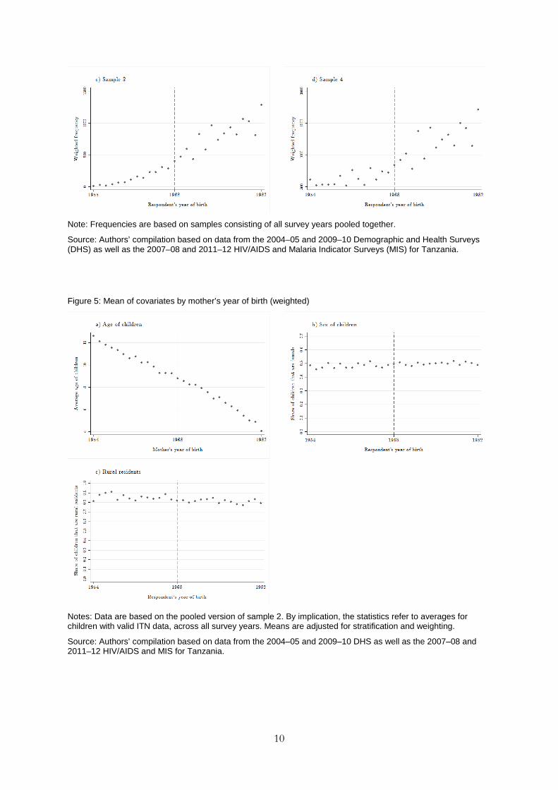
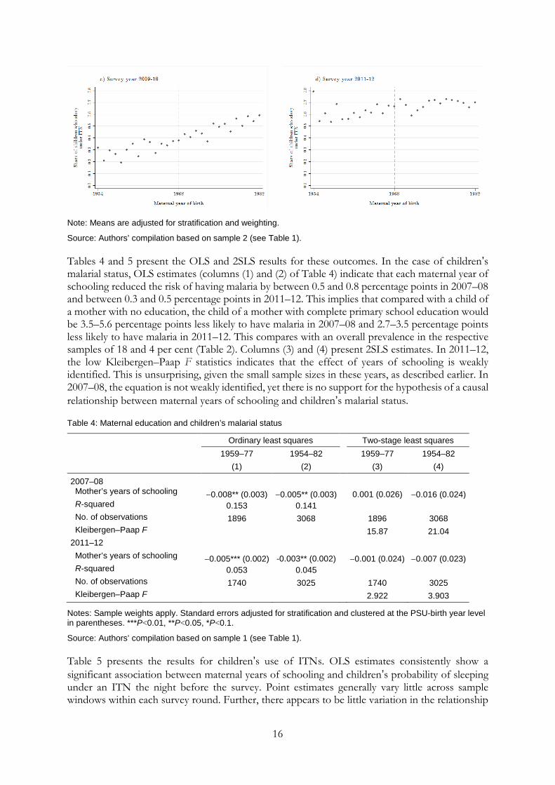
Card et al. (2015) show that requirement (b) has the testable implications that there is no kink or jump in the density of the assignment variable or the conditional distribution of any predetermined variables at the kink point. In Figure 4, we plot weighted number of observations against year of birth for each of our samples. For expositional purposes, we only present graphs based on all survey rounds pooled together. Based on this, there is no evidence of a kink or jump in the density of the assignment variable in our samples. In Figure 5, we plot the average age of children, share of children that are female, and share of children that are rural residents against maternal year of birth. Here, again for expositional purposes we present only plots based on sample 2 with all survey years pooled.6 Based on this there is no evidence of a kink or a jump in the conditional means of the covariates either. Finally, given that the predetermined covariates available from the DHS are sparse, in Figure 6 we present estimates of the under-five mortality rate, produced by UNICEF-IGME (2015), for the period covered by the birth years of women in our samples. Again, we find no evidence of a kink or jump in 1968. Thus, we have no evidence that the requirements for the RK design are not met in our case, and therefore we proceed with the RK analysis.

Figure 4: Weighted number of observations by year of birth

6 Plots for other samples and individual survey rounds are available upon request.

10

Note: Frequencies are based on samples consisting of all survey years pooled together.

Source: Authors’ compilation based on data from the 2004–05 and 2009–10 Demographic and Health Surveys (DHS) as well as the 2007–08 and 2011–12 HIV/AIDS and Malaria Indicator Surveys (MIS) for Tanzania.

Figure 5: Mean of covariates by mother’s year of birth (weighted)

Notes: Data are based on the pooled version of sample 2. By implication, the statistics refer to averages for children with valid ITN data, across all survey years. Means are adjusted for stratification and weighting.


11

Figure 6: Under-five mortality rate, 1954–82

Source: Authors’ compilation, created with estimates generated by UNICEF-IGME (2015).

Just as the fuzzy RD design in practice can be implemented through two-stage least-squares (2SLS) estimation using an indicator for the policy cut-off as the excluded instrument (see previously cited studies), the fuzzy RK design can be implemented through 2SLS using an interaction between the cut-off indicator and the running variable (essentially the slope change) as the excluded instrument (Card et al. 2012). We take this approach, and estimate first-stage regression of the form:

𝑆𝑆𝑖𝑖 = 𝛽𝛽2𝐼𝐼𝑝𝑝𝑝𝑝𝑝𝑝𝑝𝑝1968 × (𝑌𝑌𝑌𝑌𝐵𝐵𝑖𝑖 − 1968) + 𝛽𝛽3 × (𝑌𝑌𝑌𝑌𝐵𝐵𝑖𝑖 − 1968) + 𝜃𝜃𝑋𝑋𝑖𝑖 + 𝜖𝜖𝑖𝑖 (3)

where Ipost-1968 is an indicator variable that takes on the value 1 if year of birth is 1968 or later and YOB is year of birth. We use linear approximations of the relationship between birth year and years of schooling on both sides of the cut-off, which visualizations in Figures 2 and 7 suggest is a good fit. As already mentioned, we consider two different windows of (maternal) birth years, corresponding to bandwidth of 9 and 14 on either side of the cut-off. We choose bandwidths that result in intervals on either side of the kink, which inclusive of the cut-off year are divisible by five, in order to minimize potential confounding caused by age heaping.7 Predicted values, �̂�𝑆𝑖𝑖, from these regressions are then used to estimate the second stage:

𝑀𝑀𝑖𝑖 = 𝛼𝛼 + 𝛽𝛽�̂�𝑆𝑖𝑖 + 𝛾𝛾 × (𝑌𝑌𝑌𝑌𝐵𝐵𝑖𝑖 − 1968) + 𝛿𝛿𝑋𝑋𝑖𝑖 + 𝜀𝜀𝑖𝑖 (4)

7 Initially, we also considered a more restricted window based on a bandwidth of 4. However, this resulted in too small samples and insignificant first-stage results.

12

All estimations take account of the DHS/MIS set-up, which implies that we use sampling weights and adjust standard errors for both clustering and stratification. In terms of clustering, we interact the survey clusters (primary sampling units) with birth years to account for correlation of errors within birth years, across sampling units, which may result, for example, from age heaping. The coefficient β from Equation (4) can be interpreted as the weighted average marginal effect of an extra year of schooling on Mi, with weights reflecting the relative probability of being born in the cut-off year (thus proportionate to the proximity to 1968) (Card Lee et al. 2015). In that sense, to the extent that effects of schooling are heterogeneous across cohorts, it is only representative for cohorts close to the cut-off year.

Figure 7: Women’s average years of schooling and 5 year moving average rate by year of birth

13

Notes: Graphs are based on samples consisting of all survey years pooled together. Means are adjusted for stratification and weighting.


4 Results

4.1 First-stage results

Figure 7 corresponds to Figures 2 and 3, but here to DHS/MIS sample data rather than census data. This provides visual evidence, based on our estimation samples, that there is no discontinuity in the relationship between birth year and years of schooling for women in Tanzania (see condition (a)). We draw two additional conclusions based on these figures. The first is that in sample 1, the relationship between birth year and years of schooling appears less smooth than in other survey years. This may be due to the sample being relatively small, which means that averages are relatively imprecisely estimated. By implication, the RK/IV estimator may perform relatively poorly in this sample. The second observation is that based on samples 2 and 4, 1967 rather than 1968 appears to be the kink year. We chose the kink year for the analysis based on census data so as to avoid specification search. Therefore, we proceed with using 1968 as the kink year.

As noted, we consider two different birth-year windows for each sample and consider four different survey years (or two in the case of children’s malarial status). Therefore, in total, we are dealing with 28 different sub-samples of varying sizes, with 28 different first stages. Table 3 presents these first-stage regressions.

14

Table 3: Maternal birth year and educational attainment (first-stage regressions)

Maternal years of schooling, sample 1

Maternal years of schooling, sample 2

Years of schooling, sample 3

Years of schooling, sample 4

1959–77 1954–82 1959–77 1954–82 1959–77 1954–82 1959–77 1954–82 (2) (3) (2) (3) (2) (3) (2) (3) 2004–05 (Maternal) birth year

0.229*** 0.261*** 0.233*** 0.293*** 0.237*** 0.264*** (0.030) (0.017) (0.040) (0.027) (0.026) (0.014)

Slope change at birth year 1968

−0.286*** −0.323*** −0.256*** −0.341*** −0.242*** −0.289***

(0.051) (0.028) (0.059) (0.036) (0.044) (0.023)

R-squared 0.126 0.158 0.131 0.143 0.160 0.205 No. of obs. 10565 13783 2456 3766 3907 6054 2007–08 (Maternal) birth year

0.272*** 0.252*** 0.303*** 0.261*** 0.215*** 0.199*** 0.302*** 0.254*** (0.058) (0.045) (0.037) (0.021) (0.055) (0.050) (0.031) (0.015)


−0.337*** −0.259*** −0.371*** −0.289*** −0.259*** −0.198*** −0.366*** −0.262*** (0.085) (0.057) (0.060) (0.032) (0.078) (0.060) (0.050) (0.025)

R-squared 0.109 0.102 0.121 0.132 0.094 0.099 0.155 0.187 No. of obs. 1896 3068 8209 11362 1528 2453 3021 4783 2009–10 (Maternal) birth year

0.222*** 0.234*** 0.204*** 0.167** 0.226*** 0.213*** (0.039) (0.021) (0.077) (0.073) (0.031) (0.016)


−0.248*** −0.253*** −0.239** −0.159* −0.262*** −0.218*** (0.061) (0.032) (0.098) (0.082) (0.050) (0.026)

R-squared 0.121 0.140 0.125 0.132 0.153 0.191 No. of obs. 8722 12515 1496 2466 3236 5207 2011–12 (Maternal) birth year

0.214* 0.202** 0.298*** 0.255*** 0.178 0.147 0.263*** 0.248*** (0.114) (0.099) (0.037) (0.027) (0.124) (0.119) (0.026) (0.016)

Slope change birth year 1968

−0.237* −0.214** −0.356*** −0.286*** −0.210 −0.161 −0.314*** −0.267*** (0.137) (0.109) (0.056) (0.036) (0.145) (0.128) (0.045) (0.025)

R-squared 0.138 0.127 0.123 0.135 0.115 0.119 0.167 0.202 No. of obs. 1740 3025 9276 13665 1434 2435 3820 5831

Notes: obs., observations. Sample weights apply. Standard errors adjusted for stratification and clustered at the primary sampling unit–birth year level in parentheses. ***P<0.01, **P<0.05, *P<0.1.


The regressions reveal that in all but one sub-sample (sample 3, women with pregnancy in the last two years, in 2011–12), the coefficients on the instrument (slope change in 1968) are significant. This holds for both the wider (1954–82) and the narrower (1959–77) birth-year windows. There is some variation in the magnitude of the point estimate of the coefficient, which ranges between −0.159 and −0.371. In 70 per cent of the cases, however, the point estimate is between −0.3 and −0.2. Further, in all cases the slope change approximately equals the pre-1968 slope. This implies that, across samples, there was a positive relationship between (maternal) birth year and educational attainment prior to 1968, whereby the expected years of schooling increased by 0.15–0.3 for each year. After 1968, this relationship disappeared, as years of schooling became approximately constant across cohorts born later than 1968.

4.2 Education and malaria-related outcomes for children

Figures 8 and 9 plot, respectively, the share of children who have malaria and the share of children who slept under ITNs the night prior to the interview against maternal year of birth. If years of

15

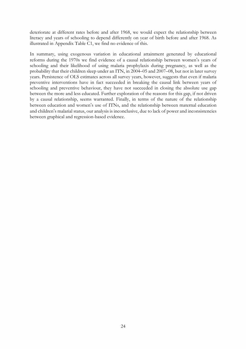
schooling have an effect on these outcomes, we would expect to see a kink in the graphs in 1968 where the relationship between years of schooling and birth year exhibits a kink. In the case of the share of children with malaria (Figure 8), there does seem to be a variation across maternal birth years up until 1968 or a few years later, at which point the variation is significantly reduced. However, it is less clear whether this gives rise to a kinked relationship and if so which year constitutes the kink point. As noted, the sample sizes available for evaluating the effect of maternal education on children’s malarial status are relatively small. Further, given that older women are less likely to have children below the age of 5 years than younger women, the sample size increases in maternal year of birth. As such, in the 2007–08 survey, the average number of children tested for malaria per birth year, for birth years five years prior to 1968 was 59, whereas it was 132 for the five years after 1968. In the 2011–12 survey, the figures were 34 and 126, respectively. It is very possible that reductions in variability across birth year are driven entirely by increases in sample size.

For the share of children who sleep under ITNs (Figure 9), there is a clearer relationship with maternal year of birth, most evident in the 2007–08 and 2009–10 surveys. Children of younger mothers (later birth years) are more likely to sleep under ITNs than children of older mothers. For the survey years 2004–05 and 2007–08, there appears to be a (barely) visible kink in the relationship in or close to 1968. Meanwhile, in 2009–10 and 2011–12 this kink is not visible.

Figure 8: Share of children with malaria by maternal year of birth

Note: Means are adjusted for stratification and weighting.

Source: Authors’ compilation based on sample 1 (see Table 1).

Figure 9: Share of children who slept under an ITN last night

16



Tables 4 and 5 present the OLS and 2SLS results for these outcomes. In the case of children’s malarial status, OLS estimates (columns (1) and (2) of Table 4) indicate that each maternal year of schooling reduced the risk of having malaria by between 0.5 and 0.8 percentage points in 2007–08 and between 0.3 and 0.5 percentage points in 2011–12. This implies that compared with a child of a mother with no education, the child of a mother with complete primary school education would be 3.5–5.6 percentage points less likely to have malaria in 2007–08 and 2.7–3.5 percentage points less likely to have malaria in 2011–12. This compares with an overall prevalence in the respective samples of 18 and 4 per cent (Table 2). Columns (3) and (4) present 2SLS estimates. In 2011–12, the low Kleibergen–Paap F statistics indicates that the effect of years of schooling is weakly identified. This is unsurprising, given the small sample sizes in these years, as described earlier. In 2007–08, the equation is not weakly identified, yet there is no support for the hypothesis of a causal relationship between maternal years of schooling and children’s malarial status.

Table 4: Maternal education and children’s malarial status

Ordinary least squares Two-stage least squares

1959–77 1954–82 1959–77 1954–82

(1) (2) (3) (4)

2007–08 Mother’s years of schooling −0.008** (0.003) −0.005** (0.003) 0.001 (0.026) −0.016 (0.024) R-squared 0.153 0.141 No. of observations 1896 3068 1896 3068 Kleibergen–Paap F 15.87 21.04 2011–12 Mother’s years of schooling −0.005*** (0.002) -0.003** (0.002) −0.001 (0.024) −0.007 (0.023) R-squared 0.053 0.045 No. of observations 1740 3025 1740 3025 Kleibergen–Paap F 2.922 3.903

Notes: Sample weights apply. Standard errors adjusted for stratification and clustered at the PSU-birth year level in parentheses. ***P<0.01, **P<0.05, *P<0.1.


Table 5 presents the results for children’s use of ITNs. OLS estimates consistently show a significant association between maternal years of schooling and children’s probability of sleeping under an ITN the night before the survey. Point estimates generally vary little across sample windows within each survey round. Further, there appears to be little variation in the relationship

17

over time. Thus, the OLS estimates consistently suggest that each additional year of schooling is associated with a 0.7–1.2 percentage point increase in a child’s probability of sleeping under an ITN. This implies that the child of a women with complete primary school education is between 4.9 and 8.4 percentage points more likely to sleep under an ITN than the child of a woman with no formal education. The stability of this relationship over time is striking in a context of significant overall increases in the use of ITNs by children (Table 2). Thus in 2004–05 only 13 per cent of children slept under an ITN whereas 67 per cent did in 2011–12.

2SLS results are presented for each survey year in columns (3) and (4) of Table 5. We find that 2SLS point estimates are significant only for the first two survey rounds. Compared with the OLS estimates, the magnitude of the 2SLS estimates appear inflated. Thus, in 2004–05 the estimates suggest that the child of a woman with complete primary school education is between 12.6 and 21.0 percentage points more likely to sleep under an ITN than the child of a mother with no education. In 2007–08, the corresponding figure is 16.8–18.9 percentage points. In this context, the interpretation of the 2SLS estimate as a local average effect is important to bear in mind. In the two latest survey rounds, 2SLS estimates are insignificant. This is unsurprising given the (lack of) graphical evidence presented. Hence, we conclude that the 2SLS results support the hypothesis of a causal relationship between maternal education and children’s use of ITNs in 2004–05 and 2007–08, but not in the later survey years.

Table 5: Maternal education and children’s use of ITNs


1959–77 1954–82 1959–77 1954–82

(1) (2) (3) (4) 2004–05 Mother’s years of schooling 0.010*** (0.002) 0.010*** (0.002) 0.030* (0.017) 0.018** (0.008) R-squared 0.182 0.181 No. of observations 10,565 13,783 10,565 13,783 Kleibergen–Paap F 36.67 129.8 2007–08 Mother’s years of schooling 0.012*** (0.002) 0.012*** (0.002) 0.024* (0.014) 0.027*** (0.010) R-squared 0.176 0.160 No. of observations 8,209 11,362 8,209 11,362 Kleibergen–Paap F 41.68 84.26 2009–10 Mother’s years of schooling 0.010*** (0.003) 0.009*** (0.002) 0.003 (0.027) −0.000 (0.015) R-squared 0.156 0.157 No. of observations 8,722 12,515 8,722 12,515 Kleibergen–Paap F 17.18 76.18 2011–12 Mother’s years of schooling 0.007** (0.003) 0.010*** (0.002) 0.011 (0.020) 0.017 (0.015) R-squared 0.043 0.042 No. of observations 9,276 13,665 9,276 13,665 Kleibergen–Paap F 33.40 67.57



18

4.3 Education and maternal malaria-related behaviour

Figures 10 and 11 plot the share of women who took antimalarials during pregnancy and the share of women who slept under an ITN the night before the survey against birth years, respectively. Figure 10 quite clearly indicates that, for the 2004–05 and 2007–08 survey rounds, the relationship between a woman’s birth year and her probability of taking antimalarials during pregnancy exhibits a kink around the same time as the relationship between a birth year and years of education. Visually there does not appear to be a kink in the relationship in the 2009–10 or the 2011–12 survey rounds, where the share of women using antimalarials during pregnancy appears to be relatively high across cohorts. As in the case with children tested for malaria, however, it must be born in mind that the sample coverage of birth years prior to 1968 is quite low in those survey rounds. This is because only births that occurred within the latest two years were covered by the survey. Thus, in fact, in the last two survey rounds, the oldest cohorts represented were born in 1960 and 1962, respectively.

The relationships in Figure 11 appear to be very similar to those in Figure 8, indicating that the relationship between women’s birth years and their use of ITNs closely resembles the relationship between maternal birth years and their children’s use of ITNs. Again, the probability of sleeping under an ITN appears to increase with age, and there is slight evidence of a kink in this relationship. Meanwhile, the position of the kink does not appear consistent across survey rounds.

Figure 10: Share of women who took antimalarials during latest pregnancy



19

Figure 11: Share of women who slept under an ITN the night before the survey



Tables 6 and 7 present the results of the OLS and 2SLS regressions. Table 6 illustrates that the OLS estimates of the association between schooling and the use of antimalarials during pregnancy are (again) remarkably consistent across both survey years and sample windows. The results indicate that, across survey rounds, each year of additional schooling is associated with an approximately 2 percentage point increase in the probability of using antimalarials during pregnancy. This should be seen in the context of an increase in the overall probability of using antimalarials during pregnancy from 50 per cent in 2004–05 to 60, 68, and 75 per cent in the 2007–08, 2009–10, and 2011–12 survey rounds, respectively. The 2SLS estimates in columns (3) and (4) of Table 6 are significant for the first two survey rounds when considering the widest sample window (although only for the second survey round when considering the narrower window). For the 2007–08 survey round the point estimates are very large, indicating that each additional year of schooling leads to an increase between 9.4 and 15.5 percentage points in the probability of using antimalarials during pregnancy. This large effect size, however, must be seen in the light of an interpretation as a local average treatment effect and of a relatively low Kleibergen–Paap F statistic. Thus, a comparison to Stock–Yogo critical values indicates between 10 and 15 per cent bias of the instrumental variable relative to the OLS estimator. For 2009–10 and 2011–12, Kleibergen–Paap F statistics are very low, and the estimated relationship is insignificant. Thus, overall, we conclude that results point towards a causal relationship between years of schooling and the use of ITNs by women in 2004–05 and 2007–08, but there is no evidence of causality for the later survey rounds.

Regression results for women’s use of ITNs are presented in Table 7. OLS estimates are significant for the first three survey rounds, but decreasing in magnitude and are essentially zero in 2011–12. This is consistent with the overall use rate increasing significantly over the period from 17 per cent

20

in 2004–05 to 23, 47, and 72 per cent in 2007–08, 2009–10, and 2011–12, respectively. The 2SLS results based on the widest birth-year window indicate a statistically significant effect of schooling on women’s use of ITNs in all but the 2004–05 survey round. However, as graphical evidence does not indicate that the relationship between women’s use of ITNs and their birth year mirrors the relationship between women’s years of schooling and their birth year, we are weary to trust that these estimates in fact reflect a causal relationship. Thus, we conclude that at best, the 2SLS estimates lend weak support to the hypothesis of a causal relationship between education and women’s use of ITNs.

Table 6: Maternal education and use of antimalarials during pregnancy


1959–77 1954–82 1959–77 1954–82

(1) (2) (3) (4) 2004–05 Years of schooling 0.020*** (0.003) 0.020*** (0.003) 0.014 (0.034) 0.037** (0.016) R-squared 0.071 0.064 No. of observations 2456 3766 2456 3766 Kleibergen–Paap F 20.30 96.98 2007–08 Years of schooling 0.019*** (0.004) 0.023*** (0.003) 0.094* (0.051) 0.145** (0.059) R-squared 0.102 0.104 No. of observations 1528 2453 1528 2453 Kleibergen–Paap F 10.76 10.86 2009–10 Years of schooling 0.018*** (0.004) 0.020*** (0.003) −0.024 (0.064) 0.037 (0.077) R-squared 0.078 0.081 No. of observations 1496 2466 1496 2466 Kleibergen–Paap F 5.759 3.732 2011–12 Years of schooling 0.020*** (0.005) 0.019*** (0.003) 0.071 (0.108) 0.066 (0.120) R-squared 0.117 0.098 No. of observations 1434 2435 1434 2435 Kleibergen–Paap F 2.006 1.592



21

Table 7: Education and maternal use of ITNs

Ordinary least squares

Two-stage least squares 1959–77 1954–82

1959–77 1954–82

(1) (2)

(3) (4) 2004–05 Years of schooling 0.009*** (0.002) 0.010*** (0.002) 0.019 (0.018) 0.014 (0.009) R-squared 0.187 0.191 No. of observations 3907 6054 3907 6054 Kleibergen–Paap F 33.19 169.5 2007–08 Years of schooling 0.007*** (0.002) 0.010*** (0.002) 0.013 (0.015) 0.023** (0.011) R-squared 0.153 0.153 No. of observations 3021 4783 3021 4783 Kleibergen–Paap F 53.28 115.3 2009–10 Years of schooling 0.005* (0.003) 0.005** (0.002) 0.056** (0.028) 0.032* (0.017) R-squared 0.101 0.106 No. of observations 3236 5207 3236 5207 Kleibergen–Paap F 27.41 75.03 2011–12 Years of schooling −0.001 (0.003) −0.001 (0.002) 0.008 (0.020) 0.027** (0.014) R-squared 0.018 0.017 No. of observations 5831 3820 5831 Kleibergen–Paap F 49.26 117.2



5 Discussion and conclusion

We found that, across all survey rounds, OLS estimates indicate statistically significant relationships of the expected sign between maternal education and all outcomes considered. Thus, children’s probability of having malaria is negatively related to their mother’s years of schooling. Their probability of sleeping under an ITN, on the other hand, is positively predicted by their mother’s years of schooling. For women, the probability of using antimalarials during pregnancy and sleeping under ITNs are both positively related to their years of schooling. Further, we found that the magnitudes of the estimated relationships are generally very consistent over time. Only in the case of women’s use of ITNs did we find that point estimates are markedly lower in later than in earlier survey years. This is remarkable, given that malaria prevalence decreased and the overall use of antimalarials and ITNs increased significantly between survey years. However, we found that support for the hypothesis of the relationships being causal in nature varied across both outcomes and survey years. We will discuss variation across these two dimensions in turn.

Considering first variation across outcomes, we focus on the first two survey rounds, so as to separate this issue from variation across years. In analyses based on the RK design, we found consistent evidence of a causal effect of years of schooling in the case of women’s use of antimalarials during pregnancy and children’s use of ITNs. Meanwhile, the point estimates of the effect were (although always high compared with OLS estimates) smaller for children’s use of

22

ITNs than for women’s use of antimalarials during pregnancy. Further, for women’s use of ITNs we found at best weak evidence of causality and point estimates that were similar to or smaller than those for children’s use of ITNs. For the relationship between maternal education and children’s malarial status, we found no evidence of causality. There may be several reasons for this pattern of results.

In the case of children’s malarial status, we cannot rule out that the failure to identify a causal effect of maternal years of schooling is related to the small sizes of the available samples compared with the relatively low frequency of malaria in the population. In the case of stronger and/or larger results for the use of antimalarials than for the use of ITNs, this explanation is less relevant. We propose two other explanations that are not mutually exclusive.

First, the difference in magnitude may simply be because the overall use rate is higher for antimalarials during pregnancy than for the use of ITNs by women and children, especially in the early survey years. Thus, relative to the use rate, the difference in magnitude of estimates across these outcomes is much smaller than it is in absolute terms. Second, the results may reflect that the relationship between education and women’s use of antimalarials is in fact of a different nature than the relationship between education and the use of ITNs. This is plausible considering that, in addition to access, the uptake of these preventive measures requires different levels of understanding and trust in health authorities. Thus, the effectiveness of sleeping under a mosquito net in preventing malaria is easy to accept, given only knowledge that malaria is caused by mosquitoes that (mainly) bite at night. In addition, sleeping under ITNs has immediate benefits as it reduces exposure to bothersome bites, and it carries no risk of side effects. Accepting preventive use of antimalarials during pregnancy as a means to prevent malaria requires a more complex understanding of biology and/or trust in public health messages that cannot be directly verified through observation by individuals. In addition, it requires knowledge that pregnant women are particularly susceptible to malaria, and trust that it will not carry side effects that are harmful to the mother or child.

That concerns about side effects is a barrier to the uptake of malaria prophylaxis during pregnancy is supported by a qualitative study of knowledge, attitudes, and practices with respect to intermittent preventive treatment in pregnancy, undertaken in Korogwe district (Mubyazi et al. 2005). This study found that women did fear side effects of the use of antimalarials during pregnancy for both themselves and their children. It seems plausible that women through education, in addition to knowledge about transmission and prerequisites for understanding the efficacy of prophylaxis, gain higher trust in the benefits of formal health care.

In Table 8, we present further evidence in support of the theory that the mechanism linking education and the use of malaria prophylaxis is different (possibly stronger) than the mechanism linking education and the use of ITNs. The estimates presented in columns (1) and (2) of Table 8 correspond to OLS estimates of an extended version of model (2), which includes control for a household wealth index reported by Filmer and Pritchett (2001). Columns (2) and (4) of Table 8 present the percentage reduction in the estimated association between years of schooling and each of the three behaviour-related outcomes from Tables 5–7, resulting from the inclusion of wealth as a covariate. We see that the point estimates for both children’s and women’s use of ITNs are reduced much more than the point estimates for women’s use of antimalarials during pregnancy. In fact, in 2004–05, the point estimates of children’s and women’s use of ITNs become insignificant when wealth is controlled for. This indicates, that the relationship between the use of ITNs and (maternal) education, whether causal or not, is mediated by wealth (which possibly proxies for access) to a much higher degree than the relationship between women’s use of antimalarials and education.

23

Table 8: OLS estimates when controlling for wealth

2004–05

2007–08 Estimate Reduction Estimate Reduction Outcomes (1) (2)

(3) (4)

Children’s use of ITNs 0.001 (0.002) −90%

0.005*** (0.002) −58% Women’s use of antimalarials 0.018*** (0.003) −10%

0.019*** (0.004) −17%

Women’s use of ITNs 0.001 (0.002) −90%

0.004** (0.002) −60%

Notes: Sample weights apply. Standard errors adjusted for stratification and clustered at the PSU-birth year level in parentheses. All estimations are based on the widest samples window, which includes birth years between 1954 and 1982. ***P<0.01, **P<0.05, *P<0.1.

Source: Authors’ compilation based on samples 2, 3, and 4 (see Table 1).

With regard to variation in results over time, given the low value of the Kleibergen–Paap F statistics in the 2009–10 and 2011–12 subsamples in Table 6, we cannot rule out that the time variance in the evidence of causality in the relationship women’s use of antimalarials in pregnancy, is entirely attributable to weak instruments in the later survey rounds. However, for children’s use of ITNs, weak instruments cannot account for the failure to identify an effect of maternal years of schooling in the later survey years. This may indicate that large-scale efforts to increase use of ITNs through mass distribution implemented in Tanzania over the last decade8 have been effective not only in raising the overall level of use but also in eradicating educational barriers to use. On the other hand, OLS estimates suggest that the absolute gap in use of ITNs between children of more- and less-educated mothers remains unchanged. Thus, to the extent that this association no longer represents a causal relationship, it must be that it remains due to third factors.

On a final note, our analysis is possibly susceptible to bias arising from the fact that educational reforms during the 1970s led to changes in the quality of schooling, as well as the quantity (Al-Samarrai and Peasgood 1998). Thus, if educational quality affects the outcomes considered, then it represents an omitted variable, possibly biasing results. Specifically, it is plausible that educational quality deteriorated at a higher rate in the early 1970s when enrolment figures rose rapidly, and then either stopped declining or declined at a lesser rate later, as, for example, educational infrastructure to some degree expanded to accommodate the increased number of students. In that case, in the 2SLS set-up, educational quality is an omitted variable in our second-stage regression, which is negatively correlated with year of birth, but positively correlated with our omitted instrument (educational quality would, on average, be decreasing less for women born after 1968). Since the omitted instrument negatively predicts years of schooling (the birth year to schooling gradient is smaller for women born after rather than before 1968), the failure to include educational quality in the second-stage regression would then lead to a downward bias on the estimated relationship between years of schooling and malaria preventive behaviour. In other words, we would be underestimating the relationship between years of schooling and malaria preventive behaviour.

While we cannot entirely rule out that such omitted variable bias influences our results, in Appendix Table C1 we present suggestive evidence that it is not a major concern. The 2004–05 and 2007–08 DHS/MIS included information on women’s literacy. If educational quality did

8 While ITNs have been subsidized and socially marketed during the entire period considered in this analysis, two mass distribution ‘catch-up’ campaigns separate the early from the late survey years. The first was implemented in 2009 and targeted children below 5 years of age. The second was implemented in 2010 and targeted all sleeping spaces not previously reached. A total of 8.7 and 18.2 million nets were distributed through these campaigns, respectively (National Malaria Control Programme et al. 2013).

24

deteriorate at different rates before and after 1968, we would expect the relationship between literacy and years of schooling to depend differently on year of birth before and after 1968. As illustrated in Appendix Table C1, we find no evidence of this.

In summary, using exogenous variation in educational attainment generated by educational reforms during the 1970s we find evidence of a causal relationship between women’s years of schooling and their likelihood of using malaria prophylaxis during pregnancy, as well as the probability that their children sleep under an ITN, in 2004–05 and 2007–08, but not in later survey years. Persistence of OLS estimates across all survey years, however, suggests that even if malaria preventive interventions have in fact succeeded in breaking the causal link between years of schooling and preventive behaviour, they have not succeeded in closing the absolute use gap between the more and less educated. Further exploration of the reasons for this gap, if not driven by a causal relationship, seems warranted. Finally, in terms of the nature of the relationship between education and women’s use of ITNs, and the relationship between maternal education and children’s malarial status, our analysis is inconclusive, due to lack of power and inconsistencies between graphical and regression-based evidence.

25

References

A’Hearn, B., J. Baten, and D. Crayen (2009). ‘Quantifying Quantitative Literacy: Age Heaping and the History of Human Capital’. The Journal of Economic History, 69(3): 783–808.

Aguero, J.M. and P. Bharadwaj (2014). ‘Do the More Educated Know More about Health? Evidence from Schooling and HIV Knowledge in Zimbabwe’. Economic Development and Cultural Change, 62(3): 489–517.

Al-Samarrai, S., and T. Peasgood (1998). ‘Educational Attainments and Household Characteristics in Tanzania’. Economics of Education Review, 17(4): 395–417.

Ambrose, E.E., H.D. Mazigo, J. Heukelbach, O. Gabone, and D.L. Mwizamholya (2011). ‘Knowledge, Attitudes and Practices Regarding Malaria and Mosquito Net Use Among Women Seeking Antenatal Care in Iringa, South-Western Tanzania’. Tanzania Journal of Health Research, 13(3): 188–95.

Anders, K., T. Marchant, P. Chambo, P. Mapunda, and H. Reyburn (2008). ‘Timing of Intermittent Preventive Treatment for Malaria During Pregnancy and the Implications of Current Policy on Early Uptake in North-East Tanzania’. Malaria Journal, 7(1): 79.

Behrman, J.A. (2015). ‘The Effect of Increased Primary Schooling on Adult Women’s HIV Status in Malawi and Uganda: Universal Primary Education as a Natural Experiment’. Social Science & Medicine, 127: 108–15.

Cameron, J., and W.H. Dodd (1970). Schools, Society and Progress in Tanzania. Oxford: Pergamont Press.

Card, D., D. Lee, Z. Pei, and A. Weber (2012). ‘Nonlinear Policy Rules and the Identification and Estimation of Causal Effects in a Generalized Regression Kink Design’. NBER Working Paper 18564. Cambridge, MA: National Bureau of Economic Research (NBER). Available at: http://www.nber.org/papers/w18564.pdf (accessed December 2017).

Card, D., D. S. Lee, Z. Pei, and A. Weber (2015). ‘Inference on Causal Effects in a Generalized Regression Kink Design’. Econometrica, 83(6): 2453–83.

Clark, D., and H. Roayer (2013). ‘The Effect of Education on Adult Mortality and Health: Evidence from Britain’. The American Economic Review, 103(6): 2087–120.

De Neve, J.-W., G. Fink, S.V. Subramanian, S. Moyo, and J. Bor (2015). ‘Length of Secondary Schooling and Risk of HIV Infection in Botswana: Evidence from a Natural Experiment’. The Lancet Global Health, 3(8): e470–7.

Filmer, D., and L.H. Pritchett (2001). ‘Estimating Wealth Effects Without Expenditure Data—Or Tears: An Application to Educational Enrollments in States of India’. Demography, 38(1): 115–32.

Gathmann, C., H. Jürges, and S. Reinhold (2015). ‘Compulsory Schooling Reforms, Education and Mortality in Twentieth Century Europe’. Social Science & Medicine, 127: 74–82.

Grossman, M. (2004). ‘The Demand for Health, 30 Years Later: A Very Personal Retrospective and Prospective Reflection’. Journal of Health Economics, 23(4): 629–36.

Landais, C. (2015). ‘Assessing the Welfare Effects of Unemployment Benefits Using the Regression Kink Design’. American Economic Journal: Economic Policy, 7(4): 243–78.

Lleras-Muney, A. (2005). ‘The Relationship Between Education and Adult Mortality in the United States’. The Review of Economic Studies, 72(1): 189–221.

26

Mathania, M.M., S.I. Kimera, and R.S. Silayo (2016). ‘Knowledge and Awareness of Malaria and Mosquito Biting Behaviour in Selected Sites Within Morogoro and Dodoma Regions Tanzania’. Malaria Journal, 15(1): 1–9.

Mazigo, H.D., E. Obasy, W. Mauka, P. Manyiri, M. Zinga, and E.J. Kweka (2010). ‘Knowledge, Attitudes, And Practices About Malaria and Its Control in Rural Northwest Tanzania’. Malaria Research and Treatment, 2010: 1–9.

Meghir, C., M. Palme, and E. Simeonova (2013). ‘Education, Cognition and Health: Evidence from a Social Experiment’. NBER Working Paper 19002. Cambridge, MA: National Bureau of Economic Research (NBER). Available at: http://www.nber.org/papers/w19002.pdf (accessed December 2017).

Minnesota Population Center (2017). Integrated Public Use Microdata Series, IPUMS-International: Version 6.5 [Dataset]. 2002 Population and Housing Census for Tanzania. Minneapolis: University of Minnesota. Available at: http://doi.org/10.18128/D020.V6.5 (accessed January 2018).

Ministry of Health and Social Welfare (2012). Tanzania Mainland National Health Accounts 2009/10, With Sub-Accounts for HIV and AIDS, Malaria, Reproductive, and Child Health. Dar es Salaam: Department of Policy and Planning, Ministry of Health and Social Welfare. Available at: http://pdf.usaid.gov/pdf_docs/pnadz607.pdf (accessed December 2017).

Ministry of Health and Social Welfare (2013). Midterm Analytical Review of Performance of the Health Sector Strategic Plan III, 2009–2015. Dar es Salaam: Ministry of Health and Social Welfare of Tanzania in collaboration with the Ifakara National Health Institute, the National Institute for Medical Research and the World Health Organisation. Available at: http://www.who.int/healthinfo/country_monitoring_evaluation/TZ_AnalyticalReport_2013.pdf (accessed December 2017).

Mubyazi, G., P. Bloch, M. Kamugisha, A. Kitua, and J. Ijumba (2005). ‘Intermittent Preventive Treatment of Malaria During Pregnancy: A Qualitative Study of Knowledge, Attitudes and Practices of District Health Managers, Antenatal Care Staff and Pregnant Women in Korogwe District, North-Eastern Tanzania’. Malaria Journal, 4(1): 31.

Mushi, P.A.K. (2009). History and Development of Education in Tanzania. Dar es Salaam: Dar es Salaam University Press.

National Bureau of Statistics – NBS/Tanzania and ORC Macro (2005). Tanzania Demographic and Health Survey 2004–05 [Dataset]. Dar es Salaam: NBS/Tanzania and ORC Macro. Available at: http://dhsprogram.com/pubs/pdf/FR173/FR173.pdf (accessed January 2018).

National Bureau of Statistics – NBS/Tanzania and ICF Macro (2011). Tanzania Demographic and Health Survey 2010 [Dataset]. Dar es Salaam: NBS/Tanzania and ICF Macro. Available at: http://dhsprogram.com/pubs/pdf/FR243/FR243.pdf (accessed January 2018).

National Malaria Control Programme, World Health Organization, Ifakara Health Institute, and the INFORM Project (2013). An Epidemiological Profile of Malaria and Its Control in Mainland Tanzania. Report funded by Roll Back Malaria and the DfID, UK. Available at: http://www.inform-malaria.org/wp-content/uploads/2014/05/Tanzania-Epi-Report-060214.pdf (accessed December 2017).

Nganda, R.Y., C. Drakeley, H. Reyburn, and T. Marchant (2004). ‘Knowledge of Malaria Influences the Use of Insecticide Treated Nets but Not Intermittent Presumptive Treatment by Pregnant Women in Tanzania’. Malaria Journal, 3(1): 42.

27

Nielsen, H.S., T. Sørensen, and C. Taber (2010). ‘Estimating the Effect of Student Aid on College Enrollment: Evidence from a Government Grant Policy Reform’. American Economic Journal: Economic Policy, 2(2): 185–215.

Njau, J.D., R. Stephenson, M.P. Menon, S.P. Kachur, and D.A. McFarland (2014). ‘Investigating the Important Correlates of Maternal Education and Childhood Malaria Infections’. The American Journal of Tropical Medicine and Hygiene, 91(3): 509–19.

Tanzania Commission for AIDS – TACAIDS, Zanzibar AIDS Commission – ZAC/Tanzania, National Bureau of Statistics – NBS/Tanzania, Office of the Chief Government Statistician – OCGS/Tanzania, and Macro International (2008). Tanzania HIV/AIDS and Malaria Indicator Survey 2007–08 [Dataset]. Dar es Salaam: TACAIDS/Tanzania, ZAC/Tanzania, NBS/Tanzania, OCGS/Tanzania, and Macro International. Available at: http://dhsprogram.com/pubs/pdf/AIS6/AIS6.pdf (accessed January 2018).

Tanzania Commission for AIDS – TACAIDS, Zanzibar AIDS Commission – ZAC/Tanzania, National Bureau of Statistics – NBS/Tanzania, Office of the Chief Government Statistician – OCGS/Tanzania, and ICF International (2013). Tanzania HIV/AIDS and Malaria Indicator Survey 2011–12 [Dataset]. Dar es Salaam: TACAIDS/Tanzania, ZAC/Tanzania, NBS/Tanzania, OCGS/Tanzania, and ICF International. Available at: http://dhsprogram.com/pubs/pdf/AIS11/AIS11.pdf (accessed January 2018).

UNESCO Institute for Statistics (n.d.). UIS.Stat. Available at: http://data.uis.unesco.org/ (accessed December 2017).

UNICEF-IGME (2015). Child Mortality Estimates. Country-Specific Under-Five Mortality Rate. UN Inter-Agency Group for Child Mortality Estimation (IGME). Available at: http://data.unicef.org (accessed 28 October 2016).

28

Appendix A: Age heaping in census data

Figure A1: Age distribution of women in the Integrated Public Use Microdata Series (IPUMS) sample of the 2002 Tanzanian census.

Source: Authors’ compilation based on data from the IPUMS sample of the 2002 Tanzanian census (Minnesota Population Center 2017).

0.00

0.01

0.02

0.03

0.04

Den

sity

0 20 40 60 80 100Age (years)

29

Appendix B: Birth year – education kink year

To the choice of 1968 as a kink year in the relationship between women’s birth year and years of schooling, we estimate, for various cut-off years and various bandwidths, local linear models with educational attainment as a function of birth year, allowing a change in slope at the cut-off year. We take the cut-off year that gives rise to the greatest slope change to be the best kink point. We examine potential kink years between 1964 and 1972, both years included. We first undertake the analysis at the level of individuals, using varying bandwidths (i.e. 4, 9, 14) that result in intervals including the cut-off year that is divisible by five, in order to minimize the influence of age heaping. We then undertake the analysis at the level of cohorts, using moving averages and bandwidth ranging from 2 to 10. In Appendix Figures B1 and B2, we plot the slope change against cut-off year, for each bandwidth. Results confirm 1968 as the kink year.

Figure B1: Interaction coefficients from regression of years of schooling on year of birth and interaction between year of birth and potential kink year, plotted against kink year for various bandwidths

Note: Sample of individuals.

Source: Authors’ compilation based on the IPUMS sample from the 2002 Tanzanian census (Minnesota Population Center 2017).

30

Figure B2: Interaction coefficients from regression of average years of schooling on year of birth and interaction between year of birth and potential kink year, plotted against kink year for various bandwidths

31

Note: Sample of moving averages.

Source: Authors’ compilation based on the IPUMS sample of the 2002 Tanzanian census (Minnesota Population Center 2017).

32

Appendix C: Literacy returns to education

The estimates in Appendix Table C1 are based on an augmented version of model (2) with literacy as the dependent variable, where years of schooling is interacted with birth year as well as with an interaction between birth year and an indicator for being born in or after 1968. In this way, returns to schooling in terms of literacy is allowed to depend linearly on year of birth, and a slope change is allowed in 1968. Irrespective of the birth-year window and the survey year considered the estimated coefficient on the slope change is insignificant and in essence zero. Thus, based on this analysis we should not be concerned about omitted variables bias stemming from the failure to control for educational quality.

Table C1: Changing literacy returns to education

2004–05

2007–08 1959–77 1954–82 1959–77 1954–82

(1) (2)

(3) (4) Years of school × year of birth −0.000 (0.001) −0.000 (0.000)

0.001 (0.001) 0.000 (0.001)

Slope change in 1968 −0.000 (0.001) −0.000 (0.001)

−0.000 (0.001) −0.000 (0.001) R-squared 0.554 0.550

0.531 0.529

No. of observations 3607 5476

2849 4077


Source: Authors’ compilation based on data from the 2004–05 Demographic and Health Survey as well as the 2007–08 Malaria Indicator Survey for Tanzania.

wider working paper 2018/9 · pdf filejel classification: i12, i20, o15 . acknowledgements:...

Documents