WIDER Working Paper 2016/115

SAMOD, a South African tax-benefit microsimulation model

Recent developments

Gemma Wright,1 Michael Noble,1 Helen Barnes,1 David McLennan,1 and Michell Mpike2

October 2016

1 Southern African Social Policy Research Insights (SASPRI), Hove, United Kingdom; corresponding author: gemma.wright@saspri.org; 2 Southern African Social Policy Research Institute (SASPRI), Cape Town, South Africa.

This study has been prepared within the UNU-WIDER project on ‘The economics and politics of taxation and social protection’.

Copyright © UNU-WIDER 2016

Information and requests: publications@wider.unu.edu

ISSN 1798-7237 ISBN 978-92-9256-159-8

Typescript prepared by Anna-Mari Vesterinen.

The United Nations University World Institute for Development Economics Research provides economic analysis and policy advice with the aim of promoting sustainable and equitable development. The Institute began operations in 1985 in Helsinki, Finland, as the first research and training centre of the United Nations University. Today it is a unique blend of think tank, research institute, and UN agency—providing a range of services from policy advice to governments as well as freely available original research.

The Institute is funded through income from an endowment fund with additional contributions to its work programme from Denmark, Finland, Sweden, and the United Kingdom.

Katajanokanlaituri 6 B, 00160 Helsinki, Finland

The views expressed in this paper are those of the author(s), and do not necessarily reflect the views of the Institute or the United Nations University, nor the programme/project donors.

Abstract: This paper provides an account of a South African tax-benefit microsimulation model—SAMOD—which has been developed for use by government over the past ten years. The two datasets that underpin the current version of SAMOD are introduced, and the model’s tax and benefit policies are described with discussion of the various data challenges and assumptions that had to be made in order to simulate them, with particular emphasis on the value-added tax policy. Simulations using the two different underpinning datasets are compared with reported administrative data. The paper concludes by highlighting three future developments for SAMOD.

Keywords: tax-benefit; microsimulation, South Africa JEL classification: C63, H24, I38

Acknowledgements: The University of Essex is thanked for granting a license to SASPRI to use EUROMOD, and for their support of the SAMOD teams over the past decade. UNU-WIDER is thanked for supporting the recent developments of SAMOD as part of the SOUTHMOD programme of work. The European Commission is acknowledged for supporting the development of EUROMOD.

1

Acronyms

CDG Care Dependency Grant

CPI Consumer Price Index

CSG Child Support Grant

COICOP Classification of Individual Consumption According to Purpose

DG Disability Grant

DSD Department of Social Development

FCG Foster Child Grant

GIA Grant in Aid

ISER Institute for Social and Economic Research, University of Essex,

LCS Living Conditions Survey

NIDS National Income Dynamics Study

NT National Treasury

OAG Old Age Grant

SAMOD A South African tax-benefit microsimulation model

SARS South African Revenue Service

SASPRI Two not-for-profit organisations – Southern African Social Policy Research Insights (registered in the UK) and Southern African Social Policy Research Institute (registered in South Africa)

SASSA South African Social Security Agency

UCT University of Cape Town

UIF Unemployment Insurance Fund

UNU-WIDER United Nations University World Institute of Development Economics Research

VAT Value-added Tax

2

1 Introduction

This working paper provides an up-to-date account of a South African tax-benefit microsimulation model called ‘SAMOD’ which has been developed for use by government over the past ten years.

Static tax-benefit microsimulation is a technique that involves applying a set of policy rules to household survey data in order to calculate individual entitlement to benefits and/or liability for taxation (see for example Mitton et al. 2000; Zaidi et al. 2009). The resulting output at individual and household level can then be analysed to provide national data on, for example, eligibility for social assistance. It also enables analysis to be undertaken to explore the impact of the tax and benefit system on levels of poverty and inequality, as well as the distributional impact on the population and on different sub-groups such as older people or children. As well as simulating current arrangements, it is possible to simulate policy reforms.

The purpose of this paper is to introduce the most recent version of SAMOD. Section 2 provides a brief account of the development of SAMOD over the past decade, with examples of how the model has been used. Section 3 describes the two datasets that underpin the current version of SAMOD. Section 4 contains an account of the different tax and benefit policies that are simulated within SAMOD Version 5.2, and the various data challenges and assumptions that had to be made in order to simulate those policies. There is a particular emphasis on Value-added tax (VAT) as this represents an innovative approach to the incorporation of the policy within the model. Section 5 presents analysis of the simulations using two different national surveys, including comparisons with reported administrative data. Section 6 concludes with a discussion about three prospective developments for SAMOD that are on the horizon.

2 About SAMOD

SAMOD is a stand-alone static tax-benefit microsimulation model.1 It is underpinned by the EUROMOD software platform which was built by Professor Holly Sutherland and colleagues at the University of Essex to simulate policies for the European Union countries (e.g. Sutherland 2001; Sutherland and Figari 2013).2 EUROMOD has been developed over a 20 year period and now comprises 28 country models (Leventi and Vujackov 2016).

The main advantages of EUROMOD which make it a particularly suitable platform for the South African model are that all the calculations are transparent and can be easily modified by the user; it is very flexible and so enables almost any type of new policy to be created; the EUROMOD software programme is constantly refined by the EUROMOD team; and there is an international community of users.

1 Other examples of South African tax and benefit microsimulation research include Adelzadeh (2007), Casale

(2010), Chitiga et al. (2010), Haarman (2000), Herault (2005), Inchauste et al. (2016), Samson et al. (2002), Samson et al. 2004), and Woolard et al. (2005).

2 EUROMOD is defined as a microsimulation model of tax and benefits system for Europe comprising a user

interface, core executable, related plug-ins and supporting documentation. It does not include source input micro-data from surveys and administrative data sources.

3

SAMOD was first developed by Professor Michael Noble and team (Dr Gemma Wright, Dr Kate Wilkinson, Dr Helen Barnes, Dr Phakama Ntshongwana) at the Centre for the Analysis of South African Social Policy (CASASP) at the University of Oxford in collaboration with Professor Holly Sutherland and the EUROMOD team at the Institute for Social and Economic Research (ISER) at the University of Essex. Additional microsimulation specialists took part in SAMOD development workshops from South Africa (Dr Charles Meth and Prof Ingrid Woolard) and the UK (Prof Jonathan Bradshaw and Dr Martin Evans). The initial project, which ran from 2006–09, was funded by the national Department of Social Development (DSD) of the Government of the Republic of South Africa, as part of a programme called ‘Strengthening Analytical Capacity for Evidence-Based Decision-Making’ which was funded by the UK Department for International Development Southern Africa. Once the first version of SAMOD had been built (Wilkinson et al. 2009; Wilkinson 2009), training sessions were undertaken by the team for members of DSD and the South African Social Security Agency (SASSA).

SAMOD was further developed by CASASP and the EUROMOD team, in collaboration with the University of the Western Cape (Wright et al. 2011). This was funded by the Programme to Support Pro-Poor Policy Development (PSPPD), a partnership programme of the Presidency, Republic of South Africa and the Delegation of the European Union. As part of that project, SAMOD was underpinned by a new microdataset: the first wave of the National Income Dynamics Study (NIDS) (Smit et al. 2010). SAMOD was then updated by CASASP using NIDS Wave 2, for SASSA.

SAMOD has been developed in its current form by Southern African Social Policy Research Insights and Southern African Social Policy Research Institute (together called SASPRI) with the support of the EUROMOD team at the University of Essex. EUROMOD has been transferred by the Essex team from an Excel interface to a new stand-alone user interface which no longer requires MS Office and its components.3 Consequently, SAMOD was converted to the new user interface and named SAMOD Version 3.0, and underpinned by the NIDS Wave 3 (2012).

Most recently, work to develop and extend SAMOD has been undertaken by SASPRI as part of a broader programme of work in collaboration with United Nations University World Institute for Development Economics Research (UNU-WIDER) and the EUROMOD team at the University of Essex, called ‘SOUTHMOD’. The SAMOD work included the updating of policies to 2015 and the preparation of a new underpinning dataset (see Section 3), production of a user manual (Barnes et al. 2015), provision of a training event for DSD and SASSA in 2015, and the preparation of this working paper. The paper is based on SAMOD Version 5.2.

There are a number of ways in which SAMOD has been used over the past decade. First, the model is used on an annual basis as a source for estimates of the number of people eligible for existing grants, both for the current year and projected for future years.

Second, SAMOD has also been used in projects for DSD, SASSA, and other government departments. This includes a study to examine the costs and distributional impact of different scenarios for the provision of social assistance for young people aged 18–24 (Altman et al. 2012; Altman et al. 2014); and a series of tax and benefit options for implementing a universal benefit for older people and a universal child benefit (unpublished and ongoing). As part of a recent study for DSD, SAMOD was ‘linked up’ to an ILO-style social budget which forecasted social spending to 2030 (OPM and CASASP 2013). Also, SAMOD was used as part of a recent cost

3 It does require Microsoft .NET Framework to be installed but this is freely downloadable and often bundled with

Windows 7 or higher operating systems.

4

benefit analysis of South Africa’s Population Census for Statistics South Africa (Stats SA) (May et al. 2013), whereby analysis of the impact of different population estimates on simulated grant eligibility was undertaken using SAMOD.

Third, SAMOD has been used in academic research to examine an income maintenance grant for working age adults (Wright et al. 2011); a caregiver’s grant (Ntshongwana 2010; Ntshongwana et al. 2010); variants of the Child Support Grant (Dinbabo 2011; Wilkinson 2010); and several benefit reforms to reduce child poverty (Whitworth and Wilkinson 2013). SAMOD has also been used to explore the impact of the whole tax and benefit system on child poverty in South Africa (Wilkinson 2010, 2011).

3 The underpinning datasets

SAMOD Version 5.2 is underpinned by two separate datasets: the Living Conditions Survey (LCS) 2008/09 (Stats SA 2011) and the National Income Dynamics Study (NIDS) Wave 4 (SALDRU 2016).

It is possible to choose which dataset to use when running the model, and to compare the results. Both datasets have advantages and disadvantages, which are highlighted in this section. Table 1 provides a summary of the two surveys in terms of their key features.

Table 1: SAMOD Version 5.2 database description

SAMOD database LCS 2008/09 NIDS Wave 4

Original name Living Conditions Survey

2008/09 version 1*

National Income Dynamics Study Wave 4 Version 1.0

Provider DataFirst and Stats SA SALDRU (2016)

Year of collection 2008/09 2014

Period of collection September 2008–August 2009 (p. 47)

September 2014–August 2015 (p. 26)

Income reference period Benchmarked to March 2009 (p. 48)

Base month is November 2014**

Sample size 25,075 households (p. 47) 11,895 households (p. 6)

Notes: * The household file is referred to as v1.1; ** See the STATA do file released with NIDS Wave 4 Version 1.0, called ‘Program 1d - Deflators_W4.do’.

Sources: For LCS 2008/09 column Stats SA (2011), For NIDS Wave 4 column Chinhema et al. (2016).

3.1 The Living Conditions Survey 2008/09

The LCS 2008/09 was undertaken by Stats SA. Version 1 of the LCS 2008/09 was used for SAMOD Version 5.2 and was obtained from DataFirst4. In addition, Stats SA supplied information on mother, father and spouse person numbers as these were not included in the publicly released data, but were needed for SAMOD.

The nationally representative LCS 2008/09 is of course now several years out of date, but it was prepared in STATA as an underpinning dataset for SAMOD in order to ascertain how well it operated as a microdataset for SAMOD, as the next version of the LCS is due to be released in

4 www.datafirst.uct.ac.za

5

early 2017 and could then be incorporated. The preparation of the code to convert the LCS 2008/09 into the necessary shape and format for SAMOD will enable the incorporation of the forthcoming LCS 2015 to take place quickly.

Data adjustment

It should be noted that Stats SA (2011) inflated the LCS food expenditure data for the purposes of their analysis (see p. 59), however this adjustment was not made for the input dataset as the assumptions made for that analysis were not appropriate for the purpose of SAMOD.5

Imputations and assumptions

A number of imputations and assumptions had to be made and are summarized here.

Head of household ID—A head of household ID variable was constructed from the relationship to head of household variable (Q16RELTOHEAD, where heads are coded as 1).6 This captured a head of household for most households. In situations when no individual in the household was coded as head of household (i.e. no individual was coded as 1), then headship was assigned to the person in the household with PersonNo=1 (as respondents had been instructed to list household members starting with the head). In situations when no individuals had been given PersonNo=1, then headship was assigned to the spouse of the (actual but absent) head according to the relationship to head of household variable (Q16RELTOHEAD).

Spouse ID (idpartner)—In situations when the spouse ID was not recorded for an individual but the relationship to head of household variable for that individual was recorded as husband/wife/partner of head, the head of household ID was assigned to the spouse ID variable for that individual. In addition, the husband/wife/partner’s ID was assigned to the spouse ID variable (if not recorded) for heads of household.

Parent ID (idparent)—Within SAMOD it is necessary to be able to identify the primary caregiver, and their spouse if they have one, for each child in the dataset. This is because the Child Support Grant is paid to the child’s primary caregiver, and the means-test is applied to the primary caregiver and their spouse if they have one. The primary caregiver does not necessarily have to be the biological parent of the child, but these were prioritised first, as described here.

The obligatory EUROMOD variable Parent ID (idparent) was used by the team to signify the primary caregiver of the child. As a first step, primary caregivers were identified as the mother of each dependent child using the biological mother ID variable (q115motherpersno). If the child’s biological mother was not present in the household then the father’s ID was assigned to the idparent variable using the biological father ID variable (q112fatherpersno). So-called ‘loose’ children (i.e. those with no mother or father ID) were dealt with using a modified version of

5 In the analysis undertaken in Stats SA (2011), food expenditure was adjusted by 1.4 in order to bring it into line

with other sales data collected by Stats SA. However, the adjustments involved numerous assumptions (see p. 59) including using a ratio of food and non-alcoholic beverage sales to non-food items for data on sales by general dealers, based on a survey undertaken every five years; an assumption that households under-report consumption on these items at the same rate; and an assumption that sales are not made to businesses. The authors decided on balance to use the unadjusted data for SAMOD.

6 This variable was an intermediate variable constructed for the purpose of creating other variables required in the

input dataset, and not as a variable for inclusion in the input dataset.

6

Ingrid Woolard’s technique that she has previously applied to identify children’s primary caregivers and spouses in the Income and Expenditure Survey (see Noble et al. 2005). Accordingly, for children for whom a primary caregiver had not yet been identified, the primary caregiver was identified as:

1. the oldest woman in the household aged 13–40 at the time of the birth of the child; and if none then;

2. the youngest woman in the household aged 41 or over at the time of the birth of the child; and if none then;

3. the oldest male in the household aged 13–40 at the time of the birth of the child; and if none then;

4. the youngest male in the household aged 41 or over at the time of the birth of the child.

At the end of this process, the only children without an assigned caregiver were those aged under 13 who are mainly categorized within the survey as head of household and where no older people are in the household. These were left unallocated.

Grant outliers—The LCS uses Classification of Individual Consumption According to Purpose (COICOP) codes for income as well as expenditure values. COICOP values for reported income from old age pensions and disability grants that were either too high or too low were set to either the maximum or minimum values respectively, of Old Age Grant (OAG) (variable poa) and Disability Grant (DG) (variable bdi) for 2009. Very high COICOP values for reported income from old age pensions were recorded under private pensions in the variable xpp.

Recorded receipt of and contributions to Unemployment Insurance Fund (UIF) (bunct and bunctyn)—Only seven cases (0.01 per cent) record receipt of UIF in Q413EMONEYFROMUIF. It is unclear whether the COICOP codes for UIF are income or contributions—they are classified as taxes and so are probably contributions. Therefore the variable bunct (recorded receipt of UIF) could not be created. In terms of the variable bunctyn (UIF contributor flag), the COICOP codes for UIF are only reported at household level so it is not possible to know who made the contributions. As a proxy, all people in employment in the household were flagged as UIF contributors, and a flag was assigned to the head of household in cases where there was not anyone in employment but a COICOP amount was recorded.

Uprating

In line with EUROMOD common practice, in order to account for any time inconsistencies between the input dataset and the policy year, uprating factors are used. Each monetary variable (i.e. each income component) is uprated so as to account for changes in the non-simulated variables that have taken place between the year of the LCS data (2009) and the years of the simulated tax-benefit systems (i.e. 2014 and 2015). Uprating factors are generally based on changes in the average value of an income component between the year of the data and the policy year.

Two different uprating factors were used in order to uprate monetary variables to the policy years 2014 and 2015 in SAMOD Version 5.2. The Consumer Price Index (CPI) was used for the majority of monetary variables (Statistics South Africa 2015a), and the change in average earnings was used for employment and self-employment income (Statistics South Africa 2015b).

7

Expenditure variables are brought into the model as a separate file and are referenced using the Defvar function. Such variables are not uprated by the conventional ‘uprate’ policy. The variables are uprated using the IlVarop function within a specific ‘expenditure’ policy described elsewhere in this paper.

3.2 National Income Dynamics Study Wave 4

NIDS Wave 4 was undertaken by the University of Cape Town and is the fourth wave of the only national panel study in South Africa (Chinhema et al. 2016).

Although designed as a panel study, a set of weights was released with the data that enable the dataset to be used as a cross-sectional, nationally representative dataset.

Specifically, the version of the NIDS Wave 4 dataset used in SAMOD Version 5.2 is NIDS Wave 4 Version 1.0 which was released in 2016 by DataFirst (SALDRU 2016). The three previous waves of NIDS had worked well as underpinning datasets for SAMOD (e.g. Wright et al. 2011).

One challenge with using NIDS is that the small sample size can result in large variations at the upper end of the income distribution in particular, depending on the treatment of outliers and anomalies. This was exacerbated by the fact that gross employment income data in NIDS had not been subjected to the rigorous data cleaning process that was undertaken by the NIDS team in order to generate their derived income variables which are net of income tax (and therefore cannot be used within SAMOD). The preparation of the gross employment income variable therefore required income imputations which are detailed below.

Another challenge was that the expenditure data was less detailed than in the LCS, and so—as will be seen in the next section—the VAT policy was only simulated in SAMOD Version 5.2 using the LCS dataset.

Data adjustment

When merging the various individual and household level files together, a number of cases were dropped, comprising non-residents and deceased individuals, plus cases in the dataset from wave 3 that could not be followed up in wave 4 for various reasons. It was not necessary to make any adjustments to the weights as a result of these dropped cases as these adjustments had already been undertaken by the NIDS team.

Sixteen cases were identified that had missing weights. On closer inspection it was identified that these individuals were all living in households that had moved out of South Africa in wave 4 and so the households were not interviewed, but the individuals themselves had successfully completed an interview. For these 16 cases with a missing weight, the weight variable (dwt) was set to zero, meaning that they are not taken into account in any analysis using the output from simulations run on NIDS wave 4 data.

Imputations and assumptions

Age (dag)—Age was imputed for 16 cases that had missing age information, using a combination of current education level, highest education level completed and year completed, relationship to head, mother/father IDs, mother’s record of child births, and occasionally other

8

information such as receipt of state pension or child grant, and employment status. For example, one case with a missing age had completed grade 11 in 2011 so could be 20, but the mother's record reports that this child was born in 1990, so was assigned the age of 24.

Gender (dgn)—Thirteen cases had missing information for gender and were recoded as unspecified as it was not possible to reliably impute this information.

Grant outliers—Values for reported income from old age pensions and disability grants that were too high were set to the maximum value of OAG and DG for 2014 in the variables poa and bdi. For cases where it was indicated that the individual was in receipt of the grant but the amount was not provided, the values were set to the maximum amount of the relevant grant.

Parent ID (idparent)—The obligatory EUROMOD variable Parent ID (idparent) was interpreted by the team to mean the primary caregiver of the child. Initially, primary caregivers were identified as the co-resident mother of each dependent child using the biological mother ID variable (w4_best_mthpid—but only if living in the household) and if no mother present then the father was identified as the caregiver using the biological father ID variable (w4_best_fthpid - but only if living in the household).

Where no direct primary caregiver identification was possible because there was no co-resident mother or father ID (‘loose’ children), the following steps were undertaken to generate idparent by indirect means:

1. Assign the head of household ID to any dependent child who is a son/daughter, step, adopted or foster child of the head of household, as determined by the relationship to head of household variable (w4_r_relhead).

2. Assign the head of household ID to any dependent child who is a grandchild, nephew/niece, cousin or great-grandchild of the head of household.

3. Assign all others to the oldest person in the household provided the oldest person is not the child themselves.

Employment income (yemwg)—The NIDS dataset contains detailed information about employment income, including variables on gross employment income7 and net employment income8. For a small number of cases, imputation was undertaken on the gross employment income variable for the main job9. The need to impute was first identified by scrutinizing scatter plots of gross and net employment income for the main job to identify outliers, where gross income was implausibly high when compared to net income, even allowing for situations where some arrears of tax might have been recouped from a particular pay cheque through the PAYE system.10 The need to impute was then more formally defined as situations where the ratio of

7 Variable em1inc relates to the respondent’s main job: ‘How much did you earn last month at your main job before

any deductions for tax, medical aid or pension?’; and an equivalent question is asked about the respondent’s second job (variable em2inc).

8 Variable em1pay relates to the respondent’s main job: ‘How much was your take-home pay last month?’; and an

equivalent question is asked about the respondent’s second job (variable em2pay).

9 In total, just 418 out of 8,455 relevant cases (unweighted) were imputed.

10 The same tests were undertaken for respondents’ second jobs (where applicable) but no major outliers were

identified and so the imputations were undertaken on employment income from first jobs only.

9

take-home pay to pre-deduction earned income was greater than 0.49; that is when gross earned income amounted to at least double the net employment income.11

Computations of the average gross to net employment income ratio were then calculated for the main job, for different occupation classes (having excluded the outlier cases). These ratios were then used to impute gross salaries from net salaries for the outliers, based on the occupation class of each outlier case.

Uprating

The CPI was used to uprate all monetary variables from 2014 to the policy year (2015 in SAMOD Version 5.2). The change in average earnings could not be used to uprate employment and self-employment income as the short period of reported data that post-dated the timepoint of NIDS Wave 4 meant that it was not possible to ascertain whether changes were being driven by seasonal fluctuation.

4 Simulating the 2015 tax and benefit system

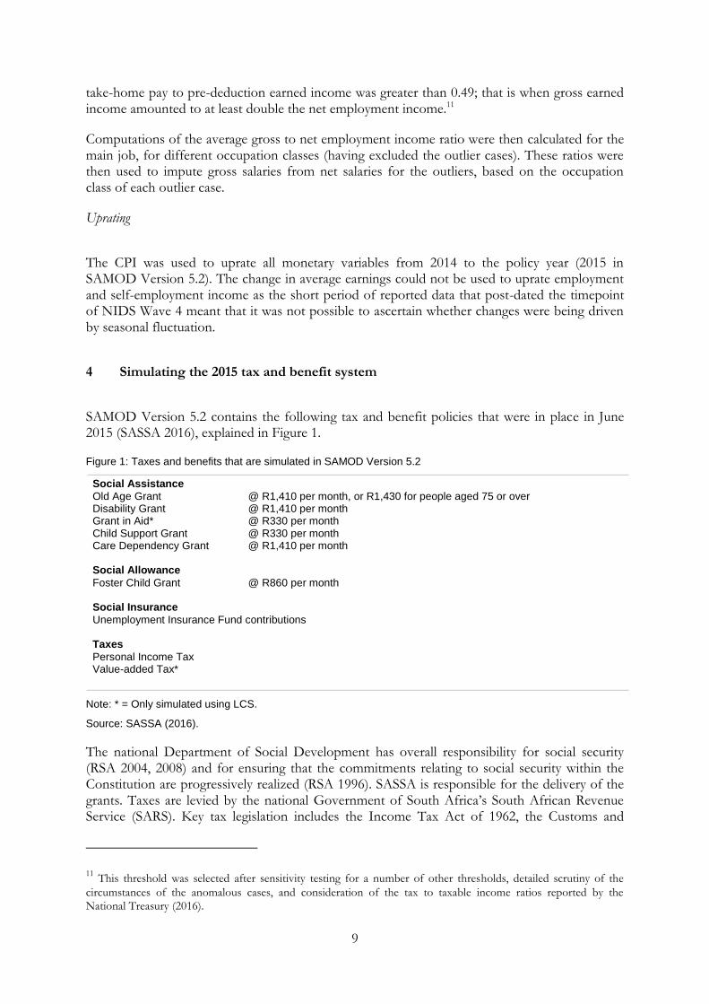
SAMOD Version 5.2 contains the following tax and benefit policies that were in place in June 2015 (SASSA 2016), explained in Figure 1.

Figure 1: Taxes and benefits that are simulated in SAMOD Version 5.2

Social Assistance

Old Age Grant @ R1,410 per month, or R1,430 for people aged 75 or over Disability Grant @ R1,410 per month Grant in Aid* @ R330 per month Child Support Grant @ R330 per month Care Dependency Grant @ R1,410 per month Social Allowance

Foster Child Grant @ R860 per month Social Insurance

Unemployment Insurance Fund contributions Taxes

Personal Income Tax Value-added Tax*

Note: * = Only simulated using LCS.

Source: SASSA (2016).

The national Department of Social Development has overall responsibility for social security (RSA 2004, 2008) and for ensuring that the commitments relating to social security within the Constitution are progressively realized (RSA 1996). SASSA is responsible for the delivery of the grants. Taxes are levied by the national Government of South Africa’s South African Revenue Service (SARS). Key tax legislation includes the Income Tax Act of 1962, the Customs and

11 This threshold was selected after sensitivity testing for a number of other thresholds, detailed scrutiny of the

circumstances of the anomalous cases, and consideration of the tax to taxable income ratios reported by the National Treasury (2016).

10

Excise Act of 1964, the Value-Added Tax Act of 1991, the Tax Administration Act of 2011 and the Employment Tax Incentives Act, 2013.

The tax and benefit policies are described briefly in this section (with reference to the timepoint of June 2015), with a particular focus on the extent to which the social security policies’ eligibility criteria could be replicated using variables contained within the LCS and NIDS datasets, and on how the personal income tax and VAT were simulated.

4.1 Social security and social insurance for adults

The Old Age Grant (OAG) is payable to low-income people aged 60 and over. The means-test threshold is R64,680 per year for single people, and R129,360 for couples, and the grant is paid on a sliding scale, from a minimum of R100 per month to a maximum of R1,410 per month. An additional payment of R20 per month is paid to those aged 75 and over. Although there is an asset test this is not applied within SAMOD as the value of people’s assets are not captured in the LCS and NIDS.

The Disability Grant (DG) is payable to low-income people aged 18–59 inclusive with a work-limiting disability. The means-test thresholds are the same as for the OAG, so R64,680 per year for single people, and R129,360 for couples, and the grant is paid on a sliding scale, from a minimum of R100 per month to a maximum of R1,410 per month. In practice, applicants must submit a medical assessment report which must not be older than three months at the date of application. The possession of such a medical assessment report is not captured in household surveys, and so proxies had to be generated for potentially eligible people. People were identified in the LCS as potentially eligible for the DG using a combination of questions relating to ability to work, chronic illness and a more general question about state of health. In NIDS, potentially eligible people were identified using a combination of questions relating to ability to work, persons who are permanently too ill and disabled to respond to the questionnaire, as well as questions relating to long term sickness or disability. Like the OAG, although there is an asset test for the DG, this is not applied within SAMOD as the value of people’s assets are not captured in the LCS and NIDS.

For those in receipt of OAG or DG and in need of full-time care due to their physical or mental disabilities, Grant-in-Aid is payable at R330 per month. Again, proxies had to be identified for those in need of full-time care. People were identified in the LCS as potentially eligible for Grant in Aid (GIA) based on information about their ability to perform tasks/undertake activities. In NIDS, potentially eligible people could not be identified as the necessary questions (or viable proxies) were not present in the questionnaire.

There is no social assistance for people of working age unless they are eligible for the DG. For those who have contributed to the Unemployment Insurance Fund (UIF) this is payable to people for a period of time for maternity leave and unemployment spells. Within SAMOD the employee and employer contributions to UIF are simulated as this type of model is not appropriate for estimating eligibility for receipt of UIF as the surveys do not provide information on employment history nor of contribution history to the UIF. Employer and employee contributions are each calculated at 1 per cent of gross salary up to a threshold salary of R14,872 per month; this is calculated for all employees who report contributions to UIF.12

12 In the case of the LCS dataset, all employees are identified as potential contributors to the UIF.

11

There is a War Veteran’s Grant which is payable at the level of R1,430 per month—either to disabled adults under 60, or adults over 60—who have a low income and fought in the Second World War or the Korean War. This grant cannot be claimed concurrently with the OAG or DG, and so in essence functions as a R20 supplement to the OAG and DG as—apart from the war veteran status—the eligibility criteria are the same as for OAG and DG, including the means test and asset test. War veteran status is not measured in either the LCS or NIDS, and so this grant is not simulated in SAMOD.

Social Relief of Distress is payable to individuals for up to three months, and a further three months in exceptional circumstances. It cannot be received in conjunction with any of the other grants and is not simulated within SAMOD as it is a short-term form of provision that is locally implemented as a response to disasters such as fire and floods.

In terms of citizenship status, OAG, DG and GIA are payable to South African citizens, permanent residents and refugees. The War Veteran’s Grant is not payable to refugees (SASSA 2016). The citizenship criteria are not applied within SAMOD.

4.2 Social security for children

The Child Support Grant (CSG) is a means-tested grant payable to the primary caregiver of a child aged less than 18. The means-test threshold for the primary caregiver’s income (and their spouse’s income if they have one) is applied at the level of R39,600 per year for single caregivers, and R79,200 per year for caregivers with a spouse. The CSG is paid at a rate of R330 per child per month. There is no cap for the number of biological children but the number of non-biological children for whom a primary caregiver makes a claim cannot exceed six. The CSG used to be unconditional but now has a ‘soft condition’ whereby children aged 7–17 inclusive have to obtain school attendance certificates, though ‘failure to produce this certificate or failure to attend school will not result in the refusal to pay their child support grant’ (SASSA 2016: 4). In practice, the soft condition and the cap for non-biological children are not applied within SAMOD.

The Foster Child Grant (FCG) is a grant payable to the primary caregiver of a child aged less than 18 who is a foster child (or aged less than 22 and still in education). It is not means-tested and so is described here as a social allowance. It is paid at the higher rate of R860 per month. In practice, it is not possible within the LCS and NIDS to identify which children ought to be in receipt of FCG—as applicants must provide a court order indicating foster care status—and so a proxy was required. Children were identified as potentially eligible if they are double orphans.13 Children aged 19-21 in education are excluded from those potentially eligible for the FCG as double orphanhood becomes a less meaningful proxy for this older age group.

The Care Dependency Grant (CDG) is a grant payable to the primary caregiver of a child aged less than 18 who is in need of care due to a permanent severe disability. This grant is paid at a higher rate of R1,410 per month. Whilst the CDG cannot be claimed concurrently with the CSG, it is possible to receive both the CDG and the FCG. In practice, children eligible for CDG had to be identified in NIDS using two different criteria as the health questions in the child questionnaire (for those aged 0–14) were different from the questions in the adult questionnaire (for those aged 15 and over). The same criteria were used for children aged 15–17 (in the adult

13 Whilst these proxies function quite well, as will be seen in the next section, it will have to be pursued differently if

a new grant for double-orphans is introduced which is currently under discussion.

12

questionnaire) as for the identification of adults aged 18–59 who are eligible for the DG. However, in the LCS, children potentially eligible for CDG were identified in the same way as for the whole age group of under 18s and using similar criteria to those used for the DG.

In terms of citizenship status, the foster carer (for FCG and CDG) or primary caregiver (for CSG and CDG) must be South African citizens, permanent residents or refugees. Both the applicant and the child must reside in South Africa (SASSA 2016). These criteria are not replicated within SAMOD.

4.3 Personal income tax

The personal income tax policy in SAMOD is one of the most complicated to implement and straddles three broad themes: the implementation of the tax rebates, the implementation of income tax on lump sums, and lastly the main income tax policy which draws the different strands together and calculates the total amount of personal income tax payable per individual in the dataset.14

The general tax rebate in 2015 was R13,257 per year, with an additional rebate of R7,407 for those aged 65 and over, and a further R2,466 for those aged 75 and above. These tax rebates are deductions from tax calculated rather than tax free thresholds.15

There are also health-insurance/health payment tax rebates though these are categorized by SARS as ‘tax credits’. The medical scheme fees tax credit amounts are calculated for the medical scheme contributor (R270 per month), their first dependant (R270 per month), and any additional dependants (R181 per month each). The eligibility for the excess medical scheme fees tax credit are also calculated, taking into account the variants to the rules for those who were aged 65 or over, and/or had a spouse or child with a disability. The total amount of tax credit is deducted from the amount of tax payable.

Deductions from the amount of tax payable in respect of donations to certain public benefit organisations are not included in SAMOD Version 5.2 as NIDS and the LCS do not contain the necessary information.

The tax on retirement related lump sums, and employment related lump sums (taking into account variants to the rules for those aged less than 55), were calculated for lump sums in excess of the threshold of R500,000 per year. The excess lump sum amounts were taxed at 18 per cent for amounts less than or equal to R200,000 per year; 27 per cent for amounts of R200,001 to R550,000 per year; and 36 per cent for amounts of R550,001 and over per year.

The calculation for the income tax policy in SAMOD Version 5.2 can be summarized as follows:

14 The tax payable is calculated at 18 per cent for the first R181,900 per year; 26 per cent for R181,901 to R284,100;

31 per cent for R284,101 to R393,200; 36 per cent for R393,201 to R550,100; 39 per cent for R550,101 to R701,300; and 41 per cent for amounts above R701,300.

15 The relationship between tax rebates and tax thresholds is as follows: all relevant income is taxed, with the first

R181,900 being taxed at 18 per cent. However the primary rebate of R13,247 is deductible from tax on income. So for example, if a person earns R73,650 they will owe SARS R73,650 x 18 per cent as personal income tax, i.e. R13,257, which is precisely the amount of the primary rebate. As the primary rebate is a deduction from tax, such a person will pay no tax. This in effect means that the tax threshold is R73,650, as people with incomes of R73,650 or below will, in practice, pay no tax.

13

Income tax payable = Tax payable on (general taxable income + income from interest payments – tax deductions for pension contributions) + Tax payable on lump sums – Tax rebate – Medical tax credits

4.4 Indirect taxes: value-added tax

Extensive work has been undertaken by the team to re-introduce VAT as a policy within SAMOD. VAT had been included in the initial version of SAMOD (Wilkinson 2009) but in that initial version aggregate groupings of expenditure items were used, whereas the intention for the most recent update was to incorporate VAT in such a way that a fine level of detail about expenditure was retained in order to maximize flexibility within the model.16 The LCS was used as it contained much finer detail on expenditure items than NIDS, and because the LCS uses an eight digit COICOP code system for expenditure items.17

VAT is described as follows by SARS:

VAT is an indirect tax on the consumption of goods and services in the economy. Revenue is raised for government by requiring certain businesses to register and to charge VAT on the taxable supplies of goods and services. These businesses become vendors that act as the agent for government in collecting the VAT.18

In South Africa the standard rate of VAT is 14 per cent, but certain goods and services are zero rated or VAT exempt.19 Zero rated items include exports, 19 basic food items20, illuminating paraffin, goods which are subject to the fuel levy (petrol and diesel), international transport services, farming inputs, sales of going concerns, and certain government grants.21 VAT exempt items include non-fee related financial services, educational services provided by an approved educational institution, residential rental accommodation, and public road and rail transport.22

The procedure for preparing the variables for SAMOD’s underpinning dataset was as follows. Expenditure data in the LCS is categorized by COICOP code23, and it was possible for each of the expenditure items to be included within the input dataset as there is no limit to the number of variables that can be included in an input file in EUROMOD. The expenditure-item-level

16 Separately, an indirect tax plug-in is being developed for EUROMOD but was not ready for use at present. In any

event, the catalyzing factor for the development of the indirect tax plug-in for EUROMOD was to enable indirect taxes to be simulated for countries whose underpinning datasets do not contain expenditure data which is not the case in South Africa (see e.g. Decoster et al. 2013).

17 In principle VAT could be simulated using NIDS, as NIDS does contain expenditure data, and so there was no

need to contemplate imputing expenditure data as is required in many countries (e.g. in Europe, Decoster et al. (2013), and in Ethiopia as part of the SOUTHMOD programme). However, as the LCS contains more detailed data on expenditure than NIDS, and as the next version of the LCS is due to be released soon, the construction of a VAT policy for the LCS dataset was prioritized.

18 See http://www.sars.gov.za/TaxTypes/VAT/Pages/default.aspx

19 See Jansen and Calitz (2015) for a recent study on the effectiveness of zero-rating of VAT in South Africa.

20 Brown bread, maize meal, samp, mealie rice, dried mealies, dried beans, lentils, pilchards/sardinella in tins, milk

powder, dairy powder blend, rice, vegetables, fruit, vegetable oil, milk, cultured milk, brown wheaten meal, eggs, and edible legumes and pulses of leguminous plants.

21 See www.treasury.gov.za/comm_media/presentations/Zero-rated%20and%20exempt%20supplies.pps

22 See www.treasury.gov.za/comm_media/presentations/Zero-rated%20and%20exempt%20supplies.pps

23 See http://unstats.un.org/unsd/cr/registry/regdnld.asp?Lg=1.

14

dataset had to be converted into a rectangular file containing one row for each household rather than multiple rows per household.

The naming convention for the expenditure variables was that each variable should start with ‘x’, followed by the eight digit COICOP code. For example the full variable name for expenditure for COICOP classification item ‘Rice’ was ‘x01111101’. A total of 748 variables were produced in this way. Having undertaken the off-model preparation of the data, further preparatory steps were undertaken within SAMOD, which are summarized in Annex 1.

The actual VAT policy was produced in SAMOD in such a way that as well as simulating the current system of VAT, two different reform scenarios could be simulated, namely one of constant consumption (assuming no change in quantities), and one of constant expenditure shares (assuming no change in expenditure shares for each type of expenditure). Put another way, the constant consumption scenario assumes that the household will spend more of its disposable income in order to purchase the same quantities of goods, whereas constant expenditure shares assume that no additional disposable income is spent, but rather that the income is spent ratably on a reduced amount of each type of expenditure. These three scenarios are summarized below.

Current system of VAT

For the current system of VAT (where the VAT rate is 14 per cent), the VAT amount was calculated as follows (see Figure 2). In lay terms, if, for example, the cost of standard rated items in a household inclusive of VAT was R114, then the temporary variable sin01_s would equal R114. The formula to calculate the amount of VAT payable is calculated as follows:

sin01_s-(sin01_s/(1+ standard rate of VAT))

For our example the amount of VAT payable would equal 114 – (114/ (1+ 0.14)) = R14. The output variable (tva01_s) is the simulated amount of VAT payable at the standard rate.

Figure 2: The ArithOp function for the current system of VAT (standard rate)

Source: Screenshot from SAMOD Version 5.2.

15

VAT reform: constant quantities

In a reform scenario where constant quantities are assumed, then it is necessary to calculate the new amount of VAT payable for a new VAT rate. In our initial example household the cost of standard rate items inclusive of VAT is R114 and so again the temporary variable sin01_s is equal to R114, but for a constant quantity scenario with a new VAT rate of 20 per cent, the amount of VAT payable is calculated as follows (see Figure 3):

(sin01_s - tva01_s) * new rate of VAT

For our example, the new rate of VAT equals 0.2. The amount of VAT payable for the example household would therefore be calculated as (114-14) *0.2 = R20.

The output variable (tvacq01_s) is the simulated amount of VAT payable at the new rate, assuming constant quantities, which for this household would be R20.

Figure 3: The ArithOp function for a reform system of VAT (20%) assuming constant quantities

Source: Screenshot from SAMOD Version 5.2.

VAT reform: constant expenditure

In a reform scenario where VAT is increased to 20 per cent and constant expenditure is assumed, then the amount of VAT payable is calculated as follows (see Figure 4):

(sin01_s/(1+ new rate of VAT)) * new rate of VAT

For our example this would be calculated as (114 / (1 + 0.2))*0.2 = 95 *0.2 = R19.

The output variable (tvacx01_s) is the simulated amount of VAT payable at the new rate, assuming constant expenditure, which for this household would be R19.

16

Figure 4: The ArithOp function for a reform system of VAT (20%) assuming constant expenditure shares

Source: Screenshot from SAMOD Version 5.2.

The VAT policy in SAMOD

The final VAT policy in SAMOD contains all three scenarios: the current system, a reform scenario assuming constant quantities and a reform scenario assuming constant expenditure. Figure 5 shows a screen shot of the final policy.

17

Figure 5: The VAT Policy in SAMOD

Source: Screenshot from SAMOD Version 5.2.

Several considerations have to be kept in mind when simulating VAT in this way, particularly—as in this version of SAMOD—where only one of the datasets can be used for simulating VAT. Our approach was to switch off all VAT related elements in the model as the default, so that the user has to actively switch them on when wishing to simulate VAT using the appropriate dataset(s). If more than one dataset can be used for simulating VAT, there would be a requirement for two (or more) DefInput functions, and the user would need to remember to switch the correct one on as otherwise the model would crash (see Annex 1).

4.5 Policies that are not simulated in SAMOD

Certain policies are not simulated in SAMOD as neither the LCS 2008/09 nor NIDS Wave 4 contained the necessary information with which to determine eligibility. This includes the War Veteran’s Grant, and Social Relief of Distress, referred to above.

Other policies are not included because the base datasets are inappropriate data sources for the type of policy in question. NIDS and LCS are household surveys, and so many of South Africa’s other taxes cannot be simulated using such datasets, including companies tax, capital gains tax, donations tax, dividends tax, turnover tax, transfer duty, estate duty, the skills development levy, fuel levy and the road accident fund.

18

Excise duties24 and ad valorem taxes are not simulated in SAMOD Version 5.2.25

Another reason for exclusion of policies is because their implementation varies by area. This includes the locally-determined indigency policies that are implemented in different ways by local government.

Additional policies that are excluded are fee free schools, free school meals, free primary health care, motor vehicle tax, road toll fees, and private and medical retirement schemes (except in so far as they impact on the personal income tax rules).

5 Results

This section presents simulations that were produced using SAMOD Version 5.2 for a June 2015 timepoint.26 As described in Section 3, SAMOD Version 5.2 is underpinned by two different datasets: NIDS Wave 4 Version 1.0 (2014 data) and LCS 2008/09. The incomes in both datasets were uprated to a 2015 timepoint but the survey weights were not recast to take into account demographic changes since the time of the survey. As explained in Section 4, GIA and VAT could not be satisfactorily simulated using NIDS data and so results are included only for the LCS for these two policies.

Table 2 shows the number of reported grant beneficiaries in June 2015 (SASSA 2015) and compares these figures with the simulated numbers of eligible beneficiaries for each grant using NIDS Wave 4 Version 1.0 and the LCS 2008/09.

For example, SASSA reported that there were 11.8 million recipients of the CSG in June 2015 whereas using SAMOD it is estimated that there were 14.9 million eligible children (using NIDS) or 13.5 million eligible children (using the LCS). This example provides a fairly stark example of the variation that can be attained from different datasets, even if the same model is used (SAMOD Version 5.2) and the very same policy rules for the CSG are applied.

24 See https://www.saldru.uct.ac.za/projects/current-projects/economics-of-tobacco-control for a recent study that

looked at excise taxes on tobacco in South Africa (amongst other things) and https://www.saldru.uct.ac.za/projects/current-projects/economics-of-alcohol-control for a current study about excise taxes on alcohol in South Africa, both at UCT.

25 These were simulated in the first version of SAMOD and will be re-introduced in due course.

26 SAMOD Version 5.2 is underpinned by EUROMOD executable version 1.12.9.

19

Table 2: Reported and simulated grant beneficiary numbers in 2015

Grant Reported (SASSA 2015)

NIDS wave 4 version 1.0 LCS 2008/09

SAMOD simulated

% captured (simulated/ reported)

Take-up (reported/ simulated)

SAMOD simulated

% captured (simulated/ reported)

Take-up (reported/ simulated)

CDG 127,869 148,931 116 86 183,555 144 70

FCG 519,031 549,336 106 94 789,343 152 66

CSG 11,792,596 14,860,987 126 79 13,511,279 115 87

OAG 3,114,729 3,838,535 123 81 3,109,370 100 100

DG 1,106,425 1,259,594 114 88 1,212,516 110 91

GIA 119,541 / / / 143,953 120 83

Source: Authors calculations using SAMOD Version 5.2 and reported figures (SASSA 2015).

Although it is not possible to state categorically which dataset provides ‘better’ estimates, the fact that NIDS Wave 4 relates to a time-point only one year prior to the policy year in question (2015) and also that (unlike the LCS) the weights in NIDS will have taken into account any recalibrations of the weights as a result of the 2011 Census of Population as well as more recent mid-year estimates, it is likely that the estimates derived from the NIDS Wave 4 data will be more reliable than from the LCS, for a 2015 time point.

In Wright et al. (2011) there is a detailed discussion about the various possible reasons for differences between reported receipt from administrative sources, reported receipt by survey respondents (not presented here), and estimates of the number of people eligible for each grant obtained from a tax-benefit microsimulation model. Clearly, the accuracy of the simulations will depend on the extent to which the survey is indeed nationally representative, the accuracy of the income and demographic data within the survey, and the precision with which the tax and benefit legislation could be replicated on-model. The reported results from administrative sources will be affected by whether there are any inclusion errors (recipients on the system who are ineligible) or exclusion errors (eligible individuals who are not registered on the system). It is important for such errors to be acknowledged before stating—for CSG—that using NIDS Wave 4 Version 1.0, 126 per cent of reported cases are simulated, implying a take-up rate of 79 per cent.

Table 3 provides the reported and the estimated (based on full take-up) cost of each grant in 2015. This is of relevance as some of the grants are payable on a sliding scale and so the costs are not necessarily straightforward multiples of the number of beneficiaries.

20

Table 3: Reported and simulated cost of grants in 2015

Grant Repor-ted

(Rm) (NationalTreasury

2016)

NIDS wave 4 version 1.0 LCS 2008/09

SAMOD simulated (R)

% captured (simulated/ reported)

Expenditure take-up

(reported/ simulated)

SAMOD simulated (R)

% captured (simulated/ reported)

Expendi-ture

take-up (reported/ simulated)

CDG 2,431 2,519,914,558 104 96 3,105,750,600 128 78

FCG 5,480 5,669,146,617 103 97 8,146,015,950 149 67

CSG 47,459 58,849,506,759 124 81 53,504,664,626 113 89

OAG 53,274 62,943,469,126 118 85 50,155,050,555 94 106

DG 19,298 21,131,594,367 110 91 19,992,457,603 104 97

Note: Official sources only report beneficiary numbers for GIA and so results for GIA costs are not included in this table.

Source: Authors calculations using SAMOD Version 5.2 and reported estimates for 2015/16 (National Treasury 2016: Chapter 5).

Table 4 provides information about the number of tax payers in 2012. The National Treasury reports just over 7 million tax payers. Using NIDS Wave 4 Version 1.0, 5.7 million tax payers are identified (81 per cent of the NT figure), compared to a much lower 5.5 million (78 per cent) using the LCS 2008/09.

Table 4: Reported and simulated number of tax payers in 2015

Reported (NT, 2016)

NIDS wave 4 version 1.0 LCS 2008/09

SAMOD simulated % captured (simulated/reported)

SAMOD simulated

% captured (simulated/reported)

2015 7,024,199 5,693,183 81 5,458,105 78

Source: Authors calculations using SAMOD Version 5.2 and reported estimates for 2015/16 (National Treasury

2016: Chapter 4).27

In terms of revenue from personal income tax, the National Treasury reported an estimate of R392 billion (see Table 5). Again, NIDS simulated tax take from personal income tax is much closer at 83 per cent of the reported figure, compared to 67 per cent using the uprated LCS 2008/09.28

Table 5: Reported and simulated revenue from personal income tax in 2015

Reported (Rm) (NT, 2016)

NIDS wave 4 version 1.0 LCS 2008/09

SAMOD simulated (Rm)

% captured (simulated/ reported)

SAMOD simulated (Rm)

% captured (simulated/ reported)

2015 392,000 326,670 83 264,138 67

Source: Authors calculations using SAMOD Version 5.2 and reported estimates for 2015/16 (National Treasury 2016: Chapter 4).

Lastly, Table 6 provides information on the tax take from VAT in 2015. The National Treasury reports a revenue of R278 billion. VAT was not simulated using NIDS, but using the LCS the simulated VAT generates 28 per cent of the reported amount. Though on the face of it this is a small amount, it should never be expected that all VAT could be simulated using a household

27 No revised estimates/actual numbers were provided in the National Treasury (2016).

28 These external validations of the simulated results compare well with those of tax-benefit models in other

countries including in Europe, e.g. in Spain (Adiego et al. 2016).

21

survey. However, it is much less than was simulated for 2008 (40 per cent) in the first version of SAMOD (Wilkinson 2009: 19).

Table 6: Reported and simulated revenue from VAT in 2015

Reported (Rm)

(NT, 2016)

NIDS wave 4 version 1.0 LCS 2008/09

SAMOD simulated % captured (simulated/ reported)

SAMOD simulated (Rm)

% captured (simulated/ reported)

2015 278,060 / / 77,042 28

Source: Authors calculations using SAMOD Version 5.2 and reported revised figure for 2015/16 (National Treasury 2016: Chapter 4).

To conclude this section, the following figure (Figure 6) shows the distributional impact of the benefits and personal income tax in 2015, based on the NIDS Wave 4.0 dataset. The figure is included here for illustrative purposes only, in order to highlight the many ways in which SAMOD can be used for research and policy to explore the impact of current policies, and options for change.

Figure 6: Distributional impact of two components of South Africa’s tax and benefit system in 2015: benefits and personal income tax

Notes: Benefits (or ‘Social Grants’) include CDG, FCG, CSG, OAG and DG. Results show benefits or personal income tax as a percentage of disposable income by income decile group. Source: Authors’ calculations using SAMOD Version 5.2 and NIDS Wave 4 Version 1.0.

6 Discussion

This working paper provides an up-to-date account of the most recent version of SAMOD—Version 5.2. SAMOD has been developed and updated for ten years, and continues to provide an important source of evidence for government for policy making purposes.

-40

-20

0

20

40

60

80

100

1 2 3 4 5 6 7 8 9 10

All Social Grants as a % ofdisposable income

Personal Income Tax as % ofdisposable income

22

In Section 3, the two datasets that underpin SAMOD—the 2008/09 Living Conditions Survey, and the 2014 National Income Dynamics Study—are described. In Section 4, the different tax and benefit policies that are included within SAMOD are described, with a particular focus on the taxes which have been developed extensively since the initial version of SAMOD was produced.

In Section 5, the simulated data is presented and compared alongside reported figures from administrative sources. SAMOD simulates personal income tax remarkably well using NIDS, and less well using the older LCS dataset even having uprated incomes using data on change in average earnings. Using the LCS, only a small proportion (28 per cent) of VAT is simulated but it is difficult to ascertain whether this is due to the quality of the expenditure data in the LCS or the fact that most VAT cannot be captured via a household survey. It is hoped that the simulated VAT will increase markedly when the new LCS is incorporated.

There are a number of ways in which SAMOD can be developed further.

First, and importantly, SAMOD is now part of an initiative to promote tax-benefit microsimulation modelling in developing countries, called SOUTHMOD which is being led by UNU-WIDER, the EUROMOD team at the University of Essex, and SASPRI. Country models are being developed for Ghana, Ecuador, Ethiopia, Mozambique, Tanzania, Viet Nam, and Zambia, as well as an update of SAMOD’s sister model in Namibia—NAMOD. It is hoped that these models will promote cross-country learning about ways in which tax and benefit systems can be used both to distribute and redistribute wealth.

Second, the process of developing SAMOD over the past decade has been an iterative and organic process. As more users become involved, and more uses for the model are identified, the policies have been and will continue to be honed and refined, as well as being updated each year to keep up with policy developments.

In addition, as part of the SOUTHMOD initiative, certain on-model analysis tools are being developed by the EUROMOD team which will be made available for incorporation into SAMOD and the other country models in 2017.

Third, the next LCS date will soon be released, which will provide a much more up-to-date data source to replace the LCS 2008/09 and a more contemporaneous comparator for the simulations obtained using NIDS Wave 4.

23

References

Adelzadeh, A. (2007). ‘Halving poverty and unemployment in South Africa: Choices for the next ten years’. In Oxfam Research Report on ‘Pro-Poor Economic Growth Models for South Africa’. Oxford: Oxfam GB.

Adiego, M., M.J. Burgos, M.M. Paniagua, and T. Perez (2016). ‘EUROMOD Country Report: Spain (ES) 2011–2015’. Colchester: University of Essex.

Altman, M., Z. Mokomane, and G. Wright (2014) ‘Social security for young people amidst high poverty and unemployment: some policy options for South Africa’. Development Southern Africa, 31(2):347–62.

Altman, M., Z. Mokomane, G. Wright, and G. Boyce (2012). ‘Social Grant for Youth—Some Policy Options: Framework on social security for youth in South Africa’. Report prepared by the Human Sciences Research Council (HSRC). Pretoria: Department of Social Development, Republic of South Africa.

Barnes, H., G. Wright, M. Noble, and M. Mpike (2015). ‘SAMOD User’s Handbook: SAMOD version 3.x’. Cape Town and Hove: SASPRI.

Casale, D. (2010). ‘Indirect Taxation and Gender Equity: Evidence from South Africa’. ERSA Working Paper 193. Cape Town: Economic Research Southern Africa.

Chinhema, M., T. Brophy, M. Brown, M. Leibbrandt, C. Mlatsheni, and I. Woolard (eds) (2016). ‘National Income Dynamics Study Panel User Manual’. Cape Town: Southern Africa Labour and Development Research Unit, University of Cape Town.

Chitiga, M., J. Cockburn, B. Decaluwe, I. Fofana, and R. Mabugu (2010) ‘Case Study: A Gender-focused Marco-Micro Analysis of the Poverty Impacts of Trade Liberalization in South Africa’. International Journal of Microsimulation, 3(1): 104–08.

Decoster, A., R. Ochman, and K. Spiritus (2013). ‘Integrating Indirect Taxation into EUROMOD: Documentation and Results for Germany’. EUROMOD Working Paper EM20/13. Colchester: University of Essex.

Dinbabo, M.F. (2011). ‘Social welfare policies and child poverty in South Africa: A microsimulation model on the child support grant’. PhD thesis. Cape Town: University of the Western Cape.

Haarman, C. (2000). ‘Social assistance in South Africa: Its potential impact on poverty’. PhD thesis. Cape Town: University of the Western Cape.

Herault, N. (2005). ‘A Micro-Macro Model for South Africa: Building and Linking a Microsimulation Model to a CGE Model’. Working Paper 16/05. Melbourne: University of Melbourne.

Inchauste, G., N. Lustig, M. Maboshe, C. Purfield, and I. Woolard (2015). ‘The distributional impact of fiscal policy in South Africa’. Policy Research Working Paper 7194. Washington, DC: World Bank.

Jansen, A., and E. Calitz (2015). ‘Reconsidering the effectiveness of zero-rating of value-added tax in South Africa’. REDI3x3 Working Paper 9. Cape Town: Southern Africa Labour and Development Research Unit, University of Cape Town.

Leventi, C., and S. Vujackov (2016). ‘Baseline results from the EU28 EUROMOD (2011–2015). EUROMOD Working Paper EM3/16. Colchester: University of Essex.

24

May, J., M. Dinbabo, J. Tamri, G. Wright, Z. Seeskin, and B. Spencer (2013). ‘Cost Benefit Analysis of South Africa’s Population Census’. Unpublished Report for Statistics South Africa.

Mitton, L., H. Sutherland, and M. Weeks (eds) (2000). Microsimulation Modelling for Policy Analysis. Cambridge: Cambridge University Press.

National Treasury (2016). ‘Budget Review 2016’. Pretoria: National Treasury South Africa.

Noble, M., G. Wright, H. Barnes, S. Noble, P. Ntshongwana, R. Gutierrez-Romero, et al. (2005). ‘The Child Support Grant: A Sub-Provincial Analysis of Eligibility and Take Up in January 2004’. Pretoria: Department of Social Development, Republic of South Africa.

Ntshongwana, P. (2010). ‘Social security provision for lone mothers in South Africa: Dependency, independence and dignity’. PhD thesis. Oxford: University of Oxford.

Ntshongwana, P., G. Wright, and M. Noble (2010). ‘Supporting Lone Mothers in South Africa: Towards Comprehensive Social Security’. Pretoria: Department of Social Development, Republic of South Africa.

OPM and CASASP (2013). ‘South Africa Social Budget: Report on the Social Budget Model and Projections’. Report. Pretoria: Department of Social Development, Republic of South Africa.

Republic of South Africa (RSA) (1996). The Constitution of the Republic of South Africa. Section 1 of 1996. Pretoria: Government Printer.

Republic of South Africa (RSA) (2004). Social Assistance Act of 2004 (Act No. 13 of 2004). Cape Town: Republic of South Africa.

Republic of South Africa (RSA) (2008). Social Assistance Amendment Act of 2008 (Act No. 6 of 2008). Cape Town: Republic of South Africa.

Samson, M., O. Babson, C. Haarman, D. Haarman, G. Khathi, K. Mac Quene, and I. van Niekerk (2002). ‘Research Review on Social Security Reform and the Basic Income Grant for South Africa’. EPRI Research Report 31. Cape Town: Economic Policy Research Institute.

Samson, M., U. Lee, A. Ndlebe, K. Mac Quene, I. van Niekerk, V. Gandhi, T. Harigaya, and C. Abrahams (2004). ‘The Social and Economic Impact of South Africa’s Social Security System’. Cape Town: Economic Policy Research Institute.

Smit, E.v.d.M., M. Leibbrandt, and G.M. Pellissier (eds) (2010). ‘Special Edition on the South African National Income Dynamics Study’. Studies in Economics and Econometrics, 34(3).

South African Social Security Agency (SASSA) (2015). ‘SASSA Fact Sheet: Issue no 6 of 2015 – 30 June 2015’. Pretoria: SASSA.

South African Social Security Agency (SASSA) (2016). ‘You and Your Grants 2016/17’. English Version. Pretoria: SASSA.

Southern Africa Labour and Development Research Unit (SALDRU) (2016). ‘National Income Dynamics Study 2014–2015’. Wave 4 [dataset]. Version 1.0. Cape Town: Southern Africa Labour and Development Research Unit [producer], 2016. Cape Town: DataFirst [distributor], 2016. Pretoria: Department of Planning Monitoring and Evaluation [commissioner], 2014.

Statistics South Africa (Stats SA) (2011) Living Conditions of Households in SA 2008/2009, Statistical Release P0310, Pretoria: Statistics South Africa.

25

Statistics South Africa (Stats SA) (2015a) Consumer Price Index August 2015, Statistical Release P0141, Pretoria: Statistics South Africa.

Statistics South Africa (Stats SA) (2015b) Quarterly Employment Statistics June 2015, Statistical Release P0277, Pretoria: Statistics South Africa.

Sutherland, H. (2001). ‘EUROMOD: an integrated European Benefit-Tax model—Final Report’. EUROMOD Working Paper EM9/01. . Colchester: University of Essex.

Sutherland, H., and F. Figari (2013). ‘EUROMOD: the European Union tax-benefit microsimulation model’. International Journal of Microsimulation, 6(1): 4–26.

Whitworth, A., and K. Wilkinson (2013). ‘Tackling child poverty in South Africa: implications of ubuntu for the system of social grants’. Development Southern Africa, 30(1): 121–34.

Wilkinson, K. (2009). ‘Adapting EUROMOD for use in a developing country—the case of South Africa and SAMOD’. EUROMOD Working Paper EM5/09. Colchester: University of Essex.

Wilkinson, K. (2010). ‘Putting children first? Tax and transfer policy and support for children in South Africa’. PhD thesis. Oxford: University of Oxford.

Wilkinson, K. (2011). ‘Modeling the impact of taxes and transfers on child poverty in South Africa’. Social Science Computer Review, 29(1): 127–44.

Wilkinson, K., G. Wright, and M. Noble (2009). ‘SAMOD User’s Handbook: Installing and running the South African Microsimulation Model’. Version 1.1. Pretoria: Department of Social Development, Republic of South Africa.

Woolard, I., C. Simkins, M. Oosthuizen, and C. Woolard (2005). ‘Final Report—Tax Incidence Analysis for the Fiscal Incidence Study being conducted for National Treasury’. Unpublished Report produced for the National Treasury, South Africa.

Wright, G., M. Noble, M. Dinbabo, P. Ntshongwana, K. Wilkinson, and P. Le Roux (2011). ‘Using the National Income Dynamics Study as the base micro-dataset for a tax and transfer South African Microsimulation Model’. Report produced for the Office of the Presidency, South Africa. Oxford: Centre for the Analysis of South African Social Policy, University of Oxford.

Zaidi, A., A. Harding, and P. Williamson (eds) (2009). New Frontiers in Microsimulation Modelling. Vienna: Ashgate.

26

Annex 1: Further details about the VAT policy

Once the LCS data on expenditure items had been prepared ‘off-model’ for incorporation into SAMOD, three steps had to be undertaken within SAMOD Version 5.2.

First, a new ‘definitional’ policy expenditure_sa is set up (see Figure A1). The definitional policy has four functions: DefVar, DefInput, DefIl and IlVarOp.

Figure A1: The expenditure_sa policy

Source: Screenshot from SAMOD Version 5.2.

The different expenditure items required for the VAT policy have to be defined within the expenditure_sa policy using the DefVar function. The following screenshot (Figure A2) shows the first 10 expenditure variables to be defined in the income list policy using DefVar.

Figure A2: An example of expenditure variables being defined (DefVar) within the expenditure_sa policy to enable VAT to be simulated

Source: Screenshot from SAMOD Version 5.2.

27

The variables were then incorporated into SAMOD using the DefInput function of the expenditure_sa policy (see Figure A3).

Figure A3: An example of expenditure variables being incorporated (DefInput) within the expenditure_sa policy to enable VAT to be simulated

Source: Screenshot from SAMOD Version 5.2.

Next, within the expenditure_sa policy, the function DefIl (define income list) was used to define an income list of items to be uprated to take into account inflation since the date of the survey. In SAMOD all items were inflated by the CPI so only one such income list was created and all items were signaled to be included by using the + sign. Figure A4 shows the first 10 items in this income list (il_exp_uprate01).

28

Figure A4: An example of expenditure variables in the income list (DefIl) to be inflated by the CPI

Source: Screenshot from SAMOD Version 5.2.

If it was decided to inflate different expenditure items by different inflators then it would be necessary to create a different income lists for different inflators. The most straightforward way to create these different income lists is to copy the entire variable list but to signal using + those items to be inflated whilst marking the others n/a.

The final function within the expenditure_sa policy is IlVarOp. The purpose of this function is to perform the arithmetical operation to inflate items within a particular income list. The following screenshot (Figure A5) demonstrates this as regards the il_exp_uprate01.

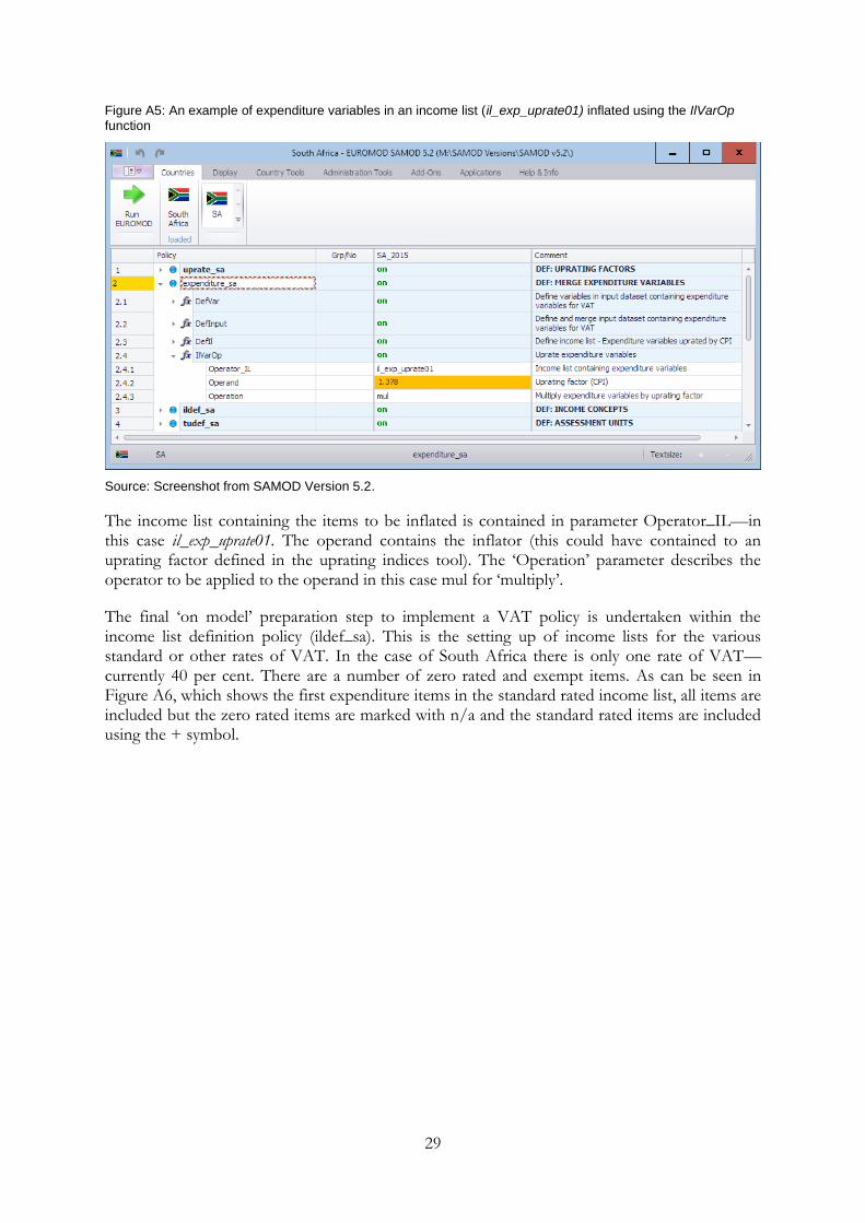
29

Figure A5: An example of expenditure variables in an income list (il_exp_uprate01) inflated using the IlVarOp function

Source: Screenshot from SAMOD Version 5.2.

The income list containing the items to be inflated is contained in parameter Operator_IL—in this case il_exp_uprate01. The operand contains the inflator (this could have contained to an uprating factor defined in the uprating indices tool). The ‘Operation’ parameter describes the operator to be applied to the operand in this case mul for ‘multiply’.

The final ‘on model’ preparation step to implement a VAT policy is undertaken within the income list definition policy (ildef_sa). This is the setting up of income lists for the various standard or other rates of VAT. In the case of South Africa there is only one rate of VAT—currently 40 per cent. There are a number of zero rated and exempt items. As can be seen in Figure A6, which shows the first expenditure items in the standard rated income list, all items are included but the zero rated items are marked with n/a and the standard rated items are included using the + symbol.

30

Figure A6: An example of expenditure variables in an income list (DefIl) to enable the standard rate of VAT to be implemented

Source: Screenshot from SAMOD Version 5.2.

This approach of using income lists means that it would be straightforward to cater for the possibility of introducing additional rates of VAT for selected items.