IEEE TRANSACTIONS ON MICROWAVE THEORY AND TECHNIQUlkS, VOL. MTT-23, NO. 2, FEBRUARY 197.5

Wide-Band Network Modeling of interacting

Inductive Irises and Steps

23.5

T. E, ROZZI AND WOLFGANG F. G. MECKLENBRAUKER

Absfracf—Methods of field and network theory are jointly applied

to he problem of deriving wide-band models for interacting in-

ductive irises and steps in standard and oversize lossless rectangular

guides.,

The resulting equivalent network is a cascade of lumped multi-

ports, described by means of @eir reactance matrix, given in the

canonical Foster% form, and of several parallel transmission lines,

connecting the interacting dkcontinuities. The required frequency

band and the accuracy of the model can be prescribed at will. The

features of the approach are: the solution of the field problem yields

a reactance matrix with monotonic convergence properties; small

matrices only need be manipulated; the frequency dependence is

explicit, so that &e field analysis need not be repeated at each fre-

quency point; a true” network model (and not a “spot frequency”

equivalent circuit) is produced, which is prerequisite for exact

synthesis.

I. INTRODUCTION

MANY standard computer oriented methods for

solving discontinuity problems in waveguide are

based on straightforward modal analysis in terms of two

finite sets of normal modes, to be matched on a certain

region, and inyersion of the resulting matrix equation [1]

A characteristic of this approach is the lack of proper

convergence with the increasing order of the double modal

expansion. Moreover, the method becomes increasingly

unsatisfactory with the number of strongly interacting

discontinuities. Quite apart from this, no proper finite

equivalent network of the discontinuity y is produced.

The importance of a proper wide-band equivalent net-

work is threefold. In the first place, such a model makes

repeating the field analysis at each frequency point un-

necessary. Secondly, a cascade of interacting discontinu-

ities can be broken down into ‘t building blocks’) connected

by transmission lines and the field problem of the whole

structure can be translated into a network problem.Thirdly, wide-band equivalent networks are prerequisite

for the exact synthesis of components and subsystems

satisfying given specifications over a given frequency band.

More anal yticall y based methods, such as the varia-

tional method [2] and the modified residue technique [3]

do not suffer from the convergence difficulties just men-

tioned. Also, simple variational and quasi-static solutions

yield equivalent circuits for isolated discontinuities in

standard guides which are often fairly accurate in a mod-

erate frequency band [4]. To date, these results are in fact

the only ones available to the microwave engineer.

Manuscript received March 20, 1974; revised July 9, 1974.The authors are with Philips Research Laboratories, Eindhoven,

The Netherlands.

However, the stringent requirements of modern telecom-

munication systems make the characterization of discon-

tinuities by means of accurate wide-band equivalent

circuits very desirable.

The principles of a variational approach, which applies

methods of both network and field theory to the problem

of lossless reciprocal discontinuities in a homogeneous

uniform waveguide, were laid ~ovm in previous contri-

butions [5]-[7].

In the present paper the approach just mentioned will

be pursued and applied to the actual derivation of wide-

band equivalent networks of interacting inductive irises

and steps in lossless rectangular guides. The guide is

standard or moderately oversize. The accuracy of the

model as well as the frequency band can be prescribed at

will.

Starting from a Rayleigh–Ritz stationary expression

for the reactance matrix pf the discontinuity y, the network

representation is derived as a finite lumped mul$iport with

frequency independent elements. In the reactance matrix

of the multiport, expressed }n the canonical Foster’s form,

the frequency dependence 1s explicit, whereas poles and

residues depend upon the geometry only. The latter de-

pendence is given in numerical or graphical form or by

means of simple interpolator functions.

The derivation of the model is based upon the follow-

ing physical considerations. In principle, a discontinuity y

excites an infinite number of modes. However, if the wave-

guide is standard or moderately oversize, only a limited

number of modes (above or below cutoff) cause appre-

ciable interaction with adj scent discontinuities. These

are the (‘accessible modes” of the discontinuity y and cor-

respond to the ‘(accessible ports” of the equivalent ~let-

work. The number of accessible modes depends, of course,

upon the accuracy required of the model. All remaining

modes, infinite in number, do not ‘(see” the rest of the

circuit; they remain confined to the neighborhood of the

discontinuity, there causing energy storage and coupling

among the accessible modes. Being well below cutoff,

localized modes are almost “lumped” in nature, whereas

accessible modes are truly ‘[distributed.” It is only natural

that accessible and localized mod,es should be treated indifferent ways, so as to suit their different properties.

The lossless reciprocal energy storage mechanism of the

localized modes is analogous to that of a cavity in all

respects [6].

The reactance matrix of an ideal Iossless cavity at its

accessible ports must satisfy Foster’s theorem. Its canon-

ical form is an infinite converging sum of resonant terms.

236 IEXETRANSACTIONS ON MICROWAVE THEORY AXD'YEC!HNIQUES, FEBRUARY 1975

L, iii L2 Iilmodes

L“’’’”’’”

Fig. 1. Cascade ofinteracting irises (top view) and equivalent net-work model.

The unknown poles and residues Fan, in fact, be extracted

from the waveguide admittance, making use of the quasi-

static character of the localized modes. This allows the

quasi-static limit of ‘the waveguide admittance to be

summed exactly for a, number of basic configurations,

whereas the dynarhic correction is a simple function of

frequency with constant’ coefficients. It will be seen that

the Rayleigh-Ritz stationary expression of order N for

the reactapce leads to a Foster’s expansion of degree 2N

Due to it: stationary nature, the latter converges rapidly

and monotonically with increasing N. Poles and residues

are related to the eigenvalues and eigenvectors of the

matrix obtained from $he waveguide admittance by means

of an appropriate’ expanding set of functions. In practice,planipulatims with matrices of small dimension only

(typically three or four) are needed.

At this point, the problem of a cascade of interacting

discontinuities is translated into the simpler network

problem of a cascade of finite m@tiports connected by

lengths af parallel transmission li~es (see Fig. 1).

‘l?he method just described will be illustrated by means

of a few numerical and experimental examples, namely,

the infinitely thin interacting iris, the thick iris, the ‘cas-

cade of thick interacting irises? and interacting steps in

rectangular waveguides.,,

II. THE SOLUTION OF THE FIELD

PROBLEM

The left-hand side of Fig. 2 illustrates the case of an

infinitely thin (a) symmetric iris at a junction of twodifferent waveguides. ‘The practically interesting cases of

the infinitely thin iris in & waveguide, the inductive step,

and the thick inductive iris are specializations or com-

binations of the preceding” configuration. These will be

treated at a later stage.

Let us consider lCaccessible modes on the left-hand sideof the diseontinuit y and li’ on the right-hand side. lia” =

k + lc’ is the total number of accessible modes of the d~s-continuity. The right-hand side of Fig. 2 shows the equiv-

alent lumped network representation of the discontinuity

as a k. port. The reference planes of the accessible modes

are placed at the Joeation oj the discontinuity. The finite

lumped rnultiport -L represents the energy storage of the

localized modes. in the neighborhood of the discontinuity.

Since the guide is uniform and lossless, coupling between

accessible modes takes place only at the location of the

discontinuity and ii described via the multiport L.

With reference to Fig. 2, let us define :“,,

r. = [(n7r/a) 2 – (27T/~)2]112, propagation constant of(1’1 = jp) the TE.O mode on th~

left-hand guide

T T’ T T’

1

n

1=— L;

k“ k’

I k+k’. keltop v,ew

Fig. 2. Geometry of basic discontinuity and its equivalent network.

I’m’ = [(mm/a’) 2 – (2m/A) 2]’/2 propagation constant of

the TE.O mode on the

right-hand guide.

The characteristic admittance of the TEno mode, nor-

malized to t$e free space admittance, is I’~/.I2wO so that the

characteristic admittance of the TE1O mode (in the larger

guide) is 13/coPo.The energy stored in the localized modes

can be computed from the susceptive part of the modified

magnetic Green’s function at z = Z1 = O. This can be

written as the sum of the contribution due to the left half-

guide and that of the right half-guide [5]. These expres-

sions can be found in a standard textbook, such as Collin’s

[8]. In our case, however, the localized modes only con-

tribute to the sum, since the accessible modes are treated

separately by means of transmission lines.

In order to obtain good convergence properties, we

transform the original kernel as described in [8,P.349]

(~ee also Appendix I). The susceptive part, normalized to

the characteristic admittance of the TE1O mode in the

larger guide, within a factor (a/m) 2 which disappears at a

later stage, is

p. and #~ are related to the cigenfunctions of the t~~-o

guides;

$%(x) = cos~ 2a

+.(X) = Cosy’ =Cos ~ (z + .rl’ — 21).

It is convenient to separate in (1) the quasi-static limit

( (a/A) 2 --+ O) and the “’dynamic correction :“

1 I’. – n7r/a+Ej ~, %(~)%(t)

n>k

ROZZI AND MECKLENBtiUKER: WIDE-BAND NETWORK MODELING 237

Further, we introduce the transformation due to T T’

Schwinger [3], [8], [9] I1

T?

1; P,A : ~,

cos~x = P1O+P11COSO := al+ a2cosok

aYk,, ,deal

trans-Y;l+ ,

with ,~-- former --,a

‘i...: L-YI I

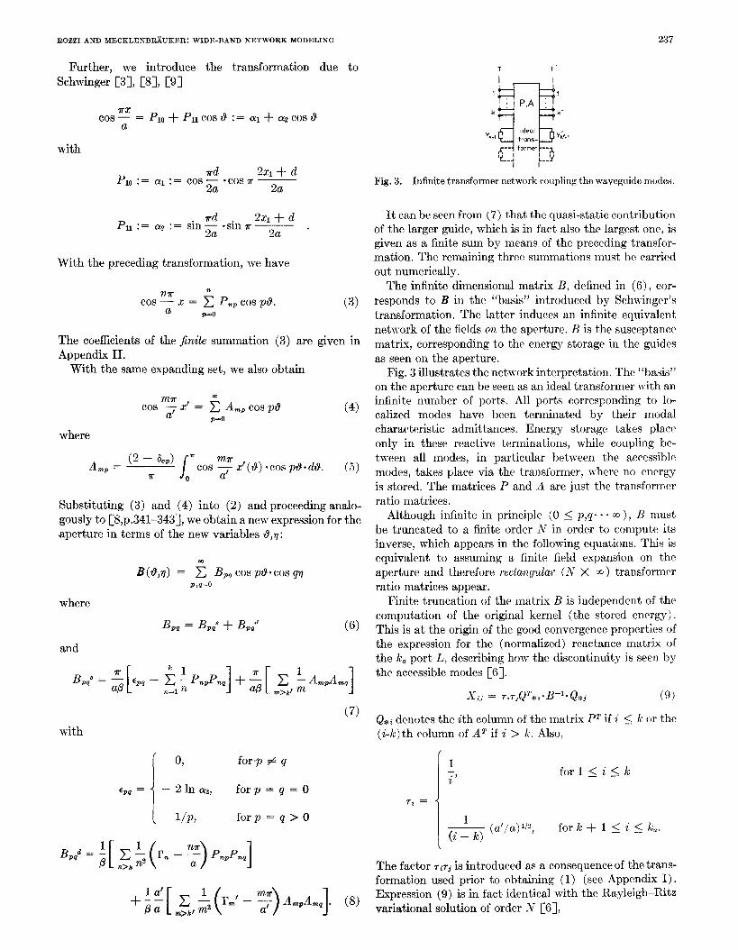
Fig. 3. Infinite transformer network coupling the waveguide modes.

.~d. 2X1 + d It can be seen from (7) that the quasi-static contributionPU : = a?

‘= ‘ln Z “sin T 2a “ bf the larger guide, which is in fact also the largest one, is

given as a finite sum by means of the preceding transfor-

With the preceding transformation, we have

n

Cos~= x = ~ P.p Cos po.a p=o

(3)

The coefficients of the jinite summation (3) are given in

Appendix II.

With the same expanding set, we also obtain

(4)

where

A =(2–M =~P JCOS‘—TX’(8) oC(X5 po. do. (.5)

T o a’

Substituting (3) and (4) into (2) and proceeding analo-

gously to [8,p.341-343], we obtain a new expression for the

aperture in terms of the new variables O,V:

B(d,v) = ~ BPg COS @“COS qq

p ,q=o

where

BP. = BP,’ + B,,d (6)

and

mation. The remaining three summations must be carried

out numerically.

The infinite ‘dimensional matrix B, defined in (6), cor-

responds to B in the (‘basis” introduced by Schwinger’s

transformation. The latter induces an infinite equivalent

network of the fields on the aperture. B is the susceptance

matrix, corresponding to th~ energy storage in the guides

as seen on the aperture.

Fig. 3 illustrates the network interpretation. The “basis”

on the aperture can be seen as an ideal transformer with aninfinite number of ports. All ports corresponding to lo-

calized modes have been terminated by their modal

characteristic admittances. Energy storage takes place

only in these reactive terminations, while coupling be-

tween all modes, in particular between the accessible

modes, takes place via the transformer, w-here no energy

is stored. The matrices P and A are just the transformer

ratio matrices.

Although infinite in principle (O S p,q o”” m), B must

be truncated to a finite order AT in order to compute its

inverse, which appears in the following equations. Thk k

equivalent to assuming a finite field expansion on the

aperture and therefore recta?wular (N X co) transformer

ratio matrices appear.

Finite truncation of the matrix B is independent of the

computation of the original kernel (the stored energy).

This is at the origin of the good convergence properties of

the expression for the (normalized) reactance matrix of

the lca port L, describing how the discontinuity is seen by

the accessible modes [6].

X’ij = TtTJQT*t . B–l . Q*j (9)

(7)Q*~ denotes the ith column of the matrix P~ if i < k or the

with (i-k) th column of AT if i > k. Also,

/

o, for p # q

% = – 2 in CX2, forp=q=O

( I/P, forp=q>O

!

1— (a’/a) ‘~’,(i – k)

fork+ l<i <km.

‘Pgd=;[zk:(rn-:) pnppql The factor riri is introduced as a consequence of the trans-

formation used prior to obtaining (1) ‘(see Appendix I).

+;;[&,#@m-~)AmpAmq]. (8) Expression (9) is in fact identical with the Rayleigh–Ritz

variational solution of order .V [6],

238 lEEETRANSACTIONS ON MICROWAVE THEORY AND TECHNIQUES, FEBRUARY 1975

III. FREQUENCY DEPENDENCE AND

FOSTER’S FORM

Localized modes are characterized by the fact that their

propagation constants are real large numbers (I’. +

n~/a, as n -+ @). Physically, this implies that the fields

pertaining to these modes remain in the neighborhood of

the discontinuity, where their excitation takes place, so

that these modes cause no interaction between neighboring

discontinuities. In intuitive terms, they do not “see” the

neighboring discontinuities. Therefore, one could imagine

that magnetic walls, for these modes only, are placed long,

but finite, distances away from the discontinuity. One

visualizes the space enclosed between these magnetic walls

and the waveguide walls as forming an ideal cavity, storing

the “energy of the localized modes. The magnetic wall

boundary conditions are consistent with a reactance

matrix description. Coupling of the cavity to the external

world takes place on the aperture of the discontinuity, via

the accessible modes.

As a function of frequency, the reactance matrix of a

lossless reciprocal cavity with lca accessible ports must

have the form

with u. z O(m) and r,j[~) * O as m ~ w. Also, the con-

stant residue matrices @J are nonnegative definite [10],

[11]. Normalization to the characteristic impedance of the

larger guide merely replaces X by ~, i.e.,

x(m) = p/wp,x(w) .

One should observe that, within a normalization constant,

(9) and (10\ are two independent expressions for the same

reactance matrix. In particular, in expression (9), ob-

tained from a waveguide description, the dependence on

the geometry and on frequency are connected in a very

complicated way. On the other hand in (10), the frequency

dependence is given explicitly, while poles and residues

are functions of the geometry only. These functions are

u~known as yet. However, they can be extracted from (9).

In the following, we shall derive from (9) a finite approxi-

mation to (10). This is based on the ‘[quasi-static” be-

havior of the localized modes and the fact that in (8) the

frequency dependence is only contained in the factors r.,

rw’, and p.

Let us now investigate the frequency dependence of the

function I’. (~)/@(ti) (n > k 2 1). We have

r.(@) 7z7r/a [1 — (l/nz) (2a/A)2]l/2

@(~) = 7r/a [(2(#A)z – 1]1/2

[1 – (fi/n) ‘]’/’

= n (fi2 _ ~],,, ~ (11)

Here we have introduced the normalized frequency & =

A,]A = 2a/A, AC= 2a being the cutoff wavelength of the

ground mode in the larger guide. With this normalization,

the ordinary guide bandwidth is given by 1 S ii s 2. To

the first two terms, the series expansion of the square root

of the numerator of (11) is

()~g1/2 162

l–— =1———.~2 2 ~2

(12)

Thk is a good approximation for (ti/n)2 <<1, as it is the

case for all localized modes except, possibly, the first few.

Furthermore, the functional form of the preceding approxi-

mation has the advantage of being very convenient for

deriving the Foster’s form of the reactance, as will be seen

later. In particular, going over to the complex frequency

p = u + ,~wit is evident that the expression

%%(;+:$)

is a positive real approximation to the input admittance of

a lossless one-port network (the characteristic admittance

of the nth mode). If only the ground mode is considered

accessible, (12) may not be always sufficient to provide a

satisfactory approximation in the frequency band of

interest.

With a view to improving the approximation while still

maintaining the convenient functional form of the right-

hand side of (12), let us slightly modify the latter as

follows :

(13)

with positive constant lcl@J, k2@J (-+ 1 as n + co ). For

given n, the free parameters kl,lc2 can be determined from

the associated problem of approximating r./@ by (nr/a)

[kl(n) – (k2(”l/2) (ti2/na) ]/@ in the Chebyshev sense over

the frequency band of interest. To give an impression of

the accuracy accruing by means of the preceding approach,

consider a typical example: n = 3, 1.2 < ti < 2. Using the

original expression (12), the maximum relative error in the

band is 1.5 percent, whereas, using (13) with ICI = 1.014,

?J2= 1.194 yields a maximum relative error equal to 1.3

per roil. The accuracy of the approximation improves

rapidly either by increasing n or reducing the frequency

band,

A similar approximation gives a fortiori better results

when applied to the

guide:propagation co~stant in the smaller

(--)1

al ; 2 1[2— (a’ < a).

a m 1

Introducing (13) in (8), we obtain from (7) and (8) the

following susceptance matrix:

B=; ~O– (Ycq (14)

where

239ROZZI AND MECKLENBRkUKER : WIDE-BAND NETWORK MODELING

[

~;(m)

+: z1

— Am@4mq (15)m>kf m

(16)

Since B is the susceptance matrix of a lossless reciprocal

structure, the matrices P and Cd are symmetric and non-

negative definite. Furthermore, the matrix @ being the

de-residue matrix of B is positive definite.

This implies in turn that the two matrices can be

diagonalized simultaneously. In order to do so, let us re-

write @ in (14) as

/3B = (0) ‘12[1 – iiz (0)-lW?(@)-’’2] (&)2/2

= (0) 1/’[1 – fi2TAT~](@) 1/2

= (0)1/27’(1 – L2A) T~(@)112(17)= M-1( I – &’A) (M-l)”

where the matrix (0) 112is the symmetric “square root” of

P, T is the orthogonal matrix of the eigenvectors of

(Cs)-’?C’(0) ‘1/2, and A is the diagonal matrix of the cor-

responding positive eigenvalues. Introducing now (17) in

(9) we obtain the (normalized) reactance matrix of the

discontinuity y as

( 18)

where A = diag ( l/ii~2). Equation (18) is the required

finite approximation to the Foster’s form (10).

As mentioned already in connection with (10), the

cavity model implies: &2 < fi22 < 00. < ~x’ = O(N’).

Furthermore, the first resonant frequency is much higher

than the upper limit of the frequency band of operation.

This is a consequence of the choice of the reference planes

and of the quasi-static behavior of the localized modes.

In (18), the frequency dependence of the reactance

matrix has been separated from the geometry dependence.

The latter is contained in the poles and the residues. Re-

peating the field analysis at each frequency point is there-

fore no longer necessary. Field analysis has provided us

with a true finite network model v slid over a prescribed

frequency band (in contrast with a “spot-frequency”Weissfloch’s equivalent circuit [8, p.251]). The study of

the frequency characteristics of the isolated discontinuity

and its interaction with other discontinuities follows now

on the basis of standard network analysis.

In the following, we shall apply the preceding theory to

the problem of buildbg an accurate network model of

waveguide components such as filters, transformers, and

cascades of inductive steps in general. We will begin with

the basic “buildlng blocks” such as the infinitely thin

symmetric inductive iris, the waveguide H-plane step, and

the thick inductive iris.

IV. THE INFINITELY THIN SYMMETRIC

INDUCTIVE IRIS IN WAVE GUIDE

A top view of the configuration is shown in Fig. 4(a),

while Fig. 4(b) gives a four-port model of the discon-

tinuity. Thk model is applicable to the case where the

TEIO mode of the guide is above cutoff, whereas the first

nonpropagating mode, the TESO mode, may still cause

appreciable interaction with neighboring discontinuities.

This choice will prove sufficient in most cases, since in

most practical situations, interaction via the first non-

propagating mode only is of any importance. The typical

range of application corresponds to an iris to iris distance

%a/2 for the worst case of higher order mode excitation

(d/a = 0.5). In fact, a two-port description is often

sufficient. This case can be easily recovered from the more

general one presented here by closing the two TEso ports

by the corresponding characteristic admittances.

The TEIO and TESOmodes are the “accessible modes” in

the sense discussed in the previous section. The remaining

TEno modes (with n odd, > 3) are the localized modes.

Since the semi-infinite guide on the left is identical to

that on the right, expressions (15) and (16) for the mat-

rices C’ and Cd in (14), now reduce to

~l(n) – 1+x PnpPng1(19)

~>3;~ odd n

and

[

~2(n)Cpqd= ? ~

1— P.pP.q .n3

(~())a n>3; n odd

One sees from (2) and Appendix I that in this case, as a

consequence of the iris being symmetric, PmP = O when-

ever p is even. At thk point, it is convenient to renumber

the indices, so that p = 2p’ – 1, q = 2q’ – 1; p’,q’ =

1,2, . . . N. N is the dimension of the finite truncation of the

matrix B, which is also the order of the finite approxima-

tion of the reactance matrk X in (10).

Symmetry about the plane z = O and reciprocity of the

structure imply that X must have the form

()xl X2

(21)

J#’ 21

where zl,zz are 2 X 2 submatrices and %1iss ymmetric. The

fact that the obstacle is infinitely thin further implies that

240 l~E~ TRANSACTIONSONMICROWAVETHEORYANDTECHNIQUES,FEBRUARY1975

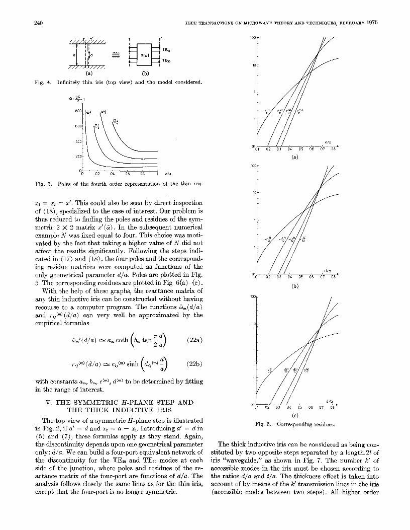
Fig. 4.

T T’

r

/

~1

a1

Id =—

II

(a) ‘

Infinitely thin iris (top

T T’

a

TEIO

x(w)T Em

100

10I

I&~800 q q

U;

600 $;

Loo :L01 02 03 OL 05 06 07 08

200 (a)

10000

02 04 06 08 1 dla [ Y /

Fig. 5. Poles of the fourth order representation of the thin iris. I Y

Z1 = x? = d. This could also be seen by direct inspection

of (18), specialized to the case of interest. Our problem is

thus reduced to finding the poles and residues of the sym- 1:

metric 2 X 2 matrix z’(;). In the subsequent numerical

example N was fixed equal to four. This choice was moti-

vated by the fact that taking a higher value of N did not

affect the results significantly. Following the steps indi-1.

cated in (17) and (18), the four poles and the correspond-

ing residue matrices were computed as functions of the

only geometrical parameter d/a. Poles are plotted in Fig.d/0

0101 02 03 OL 05 06 07 08

5 The corresponding residues are plotted in Fig 6(a)-(c).

With the help of these graphs, the reactance matrix of(b)

any thin inductive iris can be constructed without having

recourse to a computer program. The functions iifi (d/a)

and ril @@(cl/a) can very well be approximated by the

empirical formulas ’01 b

with constants am, bm, c(m), d(m) to be determined by fitting

in the range of interest.

V. THE SYMMETRIC H-PLANE STEP ANDTHE THICK INDUCTIVE IRIS

The top view of a symmetric H-plane step is illustrated

in Fig. 2, if a’ = d and X2 = a — xl. Introducing a’ = d in

(5) and (7), these formulas apply as they stand. Again,

the discontinuity depends upon one geometrical parameter

only: d/a. We can build a four-port equivalent network of

the discontinuity for the TEIO and TE30 modes at each

side of the junction, where poles and residues of the re-

actance matrix of the four-port are functions of d/a. The

analysis follows closely the same lines as for the thin iris,

except that the four-port is no longer symmetric.

(1?)

Fig. 6. Corresponding residues.

The thick inductive iris can be considered as being con-

stituted by two opposite steps separated by a length. zt of

iris “wavegnide,” as shown in Fig. 7. The number k’ of

accessible modes in the iris must be chosen according to

the ratios d/a and tla. The thickness effect is taken into

account of by means of the k’ transmission lines in the iris

(accessible modes between two steps). All higher order

ROZZIAND MECKLENB~UKER: WIDE-BAND NETWORK MODELING 241

T T’ T“/.

/

3

; l\

:

*“:@II

magnetic/electrlc wallIy

open s$c+t cmculf

(a) (b)

Fig.7. Thethlck iris asadouble step discontinuity.

(a) (b)

Fig.8. Even/odd mode problems forthethlck iris.

iris modes excited by the steps are terminated by their

characteristic admittances, i.e., they do not ‘[see” the

other step.

We can build an alternative model for the thick iris in a

waveguide since this structure is symmetric with respect

to z = O and can be analyzed in terms of the even and odd

excitation modes. The even and odd mode half-structures

are obtained by placing a magnetic or an electric wall at the

plane of longitudinal symmetry falling in the middle of the

iris, as shown in Fig. 8. This is in fact a step problem where

the modes on the right are terminated by an open/short

circuit after a distance tof transmission line.

Accordingly, the admittance matrix B for the even/odd

mode is given by the formulas (7) and (8) where for all

localized modes in the iris I’~’/B is now replaced by

Itanh r~’t

rm’/Pcoth rm’t

for the even/odd mode, respectively.

Again, owing to the weak frequency dependence of the

localized modes, we can approximate

!tanh I’~’t

I’m’

coth 17m’t

by an expression like (13), where .kl.,o’ @@,kz, ,0’t’@ (+1

as m ~ co) are determined by a Chebyshev approxi-

mation in the band of interest, for the even and odd mode

separately. The resulting expressions for the matrices C*

and Cd are

~L ,,=1 ,3 ‘{L

--~l(n) – 1

+ En7t>2k-l;n odd

+A~pA.,

x———?n>2kt-l; m odd m

PnvPnq

I 1?cI,d(m)tanh (mm/d) t

(23)

k,,o’c@ coth (mm/d) t

.{ I (24)

((lcz,o’(m) coth ~ t–m~t/d

sinhz (m7r/d) t )]

The upper expression holds for the even case, the lower one

for the odd case. Obscrve that for zt/d >>1 the expressions

for the even and odd case in (23) and (24) approach their

common value given by (1.5) and (16), respectively (set

d = a’). Starting from (23), (24), we can repeat the same

steps as in Section III, leading from (14) to (18). We thus

~btain the reactance matrices X.’, X~’ of the le.-port

representation, shown in ??ig. S(a), at the reference planes

T – T’.

If no iris mode is above cutoff, then k’ = O in the above

formulas and km = 1;.If some iris modes are above cutoff,

we can eliminate them from the network representation by

closing them with the appropriate terminations. Standard

network analysis yields the following formulas for the

k X k driving point reactance matrices X&, at the

reference planes T:

[

Xw = (Zti’)ll – (J&’) 1,” ($?4’)22

({tanh I’<t

+ ~ diag I’1’ . . . >coth rl’t ‘

I )1tanh (1’’y~~_d) -1

. r’W_l (XJ)12T (2.5)

coth (r’z~t_lt)

where

“=::(R)u stands for e in the even case and the upper expressions in

(25) should be used, u stands for o in the odd case and thelower expressions should be used.

Finally, the 2k X Ye reactance matrix of the thick iris

can be expressed in terms of the even/odd mode lC X lC

reactance matrices as

(x, + x. x, – x.

x=-: ) (26)d xeT _ ~yoT Xe + .~o

The approach just described entails repeating the analysis

for the even and the odd cases. Furthermore, poles and

residues of the reactance matrices X.,-Z are now (weak)

242 lEEKTRANSACTIONS (>NMICRO\VAVE THEORY AND TECHNIQUES, FEBRUARY 1975

functions of t/a as well as of d/a, whereas in the case of the

step, the only geometrical parameter was d/a. With respect

to the double step approach previously discussed, the ad-

vantage of the latter approach consists in the fact that

fewer accessible ports need be considered in the case of thin

irises, which is the one most frequently encountered in theapplications. In particular, if the iris is below cutoff, then

no mode at all need be Considered as accessible in the iris.

The port reduction expressed by formula (2.5) is then no

longer necessary.

An example of the latter will be discussed in the follow-

ing section.

VI, FURTHER NUMERICAL AND

EXPERIMENTAL RESULTS

The application of the theory presented in the previous

sections will now be demonstrated by means of a few

examples.

1) The Isolated Thick Iris in the Standarcl Wave@le

Band (1 < ~ < 2): Table I gives poles and residues of the

even and odd mode reactance for d/a = 0.,5 and 2t/a =

0.5. Although fairly typical in practice, these dimcmsions

represent a “worst case” for the existing approximate

representations of the iris. In fact, the preceding ratio d/a

corresponds’ to maximum higher o~der mode excitation

and the thickness, while being too large to be ‘neglected; is

at the same’ time too small to be taken care of by m~ans of

a single iris mode. In the computation, no accessible mo”des

were assumed in the iris [k’ = O in (23), (24)]. Also, .1-

vvas set equal to 3 in (18) and only one accessible mode was

assumed in the guide (k = 1). Table I shows how rapidly

the Foster’s representation converges. Only the first

resonant frequency of the even mode ‘needs be taken into

account. The contribution of all other terms can be lumped

in static inductances.The equivalent network of Fig. 9(a), is based upon the

approximation just mentioned. It holds in the ranges:

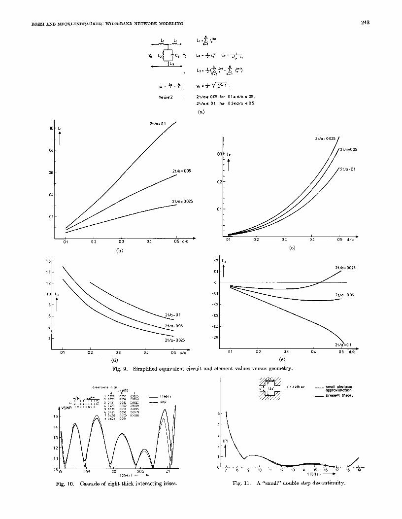
0.1 S d/a S 0.5 for 2t/a S 0.0.5 and 0.2 S cl/a 50.5 for2t/a < 0.1.

In Fig. 9 (b) – (e) the element values of Fig. 9(a) are

plotted in the preceding range. Outside this range; more

than one resonant frequency (or no resonant frequency)

need be taken into account. hTegative inductances Ls,

together with positive inductances Ll, can be interpreted

as belonging to a realizable transformer (Ll + 2Ls > O).

This occurs due to the thickness effect.2) A Cascade of Thick Interacting Inductive Irises: The

field problem of a cascade of interacting irises has been

reduced to the network problem of analyzing a cascade of

lumped multiports connected by a finite and (small)

number of transmission lines, as shown in Fig. ‘1.

In the range of interest, the multiports are described by

their canonical Foster’s form, explicitly displaying the

frequency dependence. Poles and residues depend upon the

geometry only and are obtained by means of field analysis.

Propagation constants and characteristic admittances of

the transmission lines, describing the accessible modes, are

known. Therefore, we can apply standard network analysis

TABLE I

m 1 2 3

:T: )

$!.27 51.7’7 233.38

0.630 0.0234 0.00506

gUJ~2

724.19 244.94 459.05~(m) 0.0108 0.0318 0.0154

frequency band: 1 <a < 2 (~ . 1: cutoff TEIO; ~ = 2: cutoff T~

in order to obtain the frequency characteristics of the

cascade. In order to check the theory, an accurate experi-

mental structure, consisting of a cascade of “eight inter-

acting irises, was built and tested. hTumerical and experi-

mental results are shown in Fig. 10. The figure shows

VSWR versus frequency in the range 19-21 GHz. The

thinner line was computed with the thick iris approach

described in the previous section. A fourth order trial ”field

(N = 4) was assumed on all apertures. Two modes: TE1o,

above cutoff, and TEsO, below ctitoff, but still causing

interaction, were considered accessible in the sections of

waveguide. One mode: TE1O, below cutoff, was assumed

accessible in the iris, in the even/odd mode representationof the iris. Taking N equal to 3, 5, or 6 changed the charac-

teristics only slightly. This is a consequence of the sta-

tionary nature of the reactance of each iris. The thicker

line is the envelope of experimental points obtained by

slotted-line measurements. The agreement can be con-

sidered excellent for a structure of this complexity. The

3-percent error in bandwidth and the slight peak deformat-

ion appearing at the upper band edge can be attributed to

tolerance variations in the guide width along the structure,

since the guide width was assumed constant in the com-

putation. Alsoj no account was taken of losses and of

residual geometrical imperfections such as asymmetries,

misalignment, and bending of the irises.

Interaction between adjacent irises via the TEw mode

is a relatively weak effect in the structure just mentioned.

The influence of interaction between adjacent discon-

tinuities will be illustrated in the following examples,

where the effects appear in increasing measure.

3) H-Plane Oversize Section: Consider Fig. 11. The

continuous line represents the computed modulus of thereflection coefficient for the TEIO mode versus frequency

of an H-plane oversize section in a standard X-bandxvaveguide. ‘The dimensions are given in the -figure. The

reader is cautioned that, consistent with the previous use,

a’ denotes the width of the smaller guide. As it happens, a’,.is now the standard waveguide width. The frequency

ranges from 6.5 to 19 GHz. Above this frequency (namely,

at 19.7 GHz ), the TE~o mode in the standard guide be-

comes propagating and a two-port” model for the input–

output relation nQ longer applies.

A sixth order trial field was assumed on the aperture.

Two modes were considered accessible in both sections of

ROZZIANDMECKLENBRhKER: WIDE-BANDNETWORKMODELING 243

,, .? ,))

--J-#+ ‘“

10 - L,

-t

m -

06-

OL -

02-

1*!3*2 , 2t/as 005 for Ol<d/a <05,

2t/a< 01 for 02sd/a <05,

(a)

2t/a. ol

Zth =005

2t/a=0025

I , I , I

01 02 03+

04 05 d/a

16 -

7L -

12 -

10 - C2

8

-1

6 -

L -

2 -

(b)

~=ol2t/a. oo5

2t/a. 0025

(c)

02 LS

-t2t/a=oo25

01

0

-01 - 2t/a. oos

-02 -

-03 -

-OL -

-05 -2t/i’= 01

, , I , 1 I

01 02 03 OLD ●

05 d/a 01 02 03 OL 05 d/a

(d) (e)

Fig. 9. Simplified equivalent circuit and element values versus geometry.

d,m, ns, ons m cm..1075 G

Y 2“”G, 120,

.,= 2286 cm — small obstaclea~roxl mat ton

A — “’S*’ ‘“WY

ik--L78910111213 IL 16 17 18 19

flG~5zl —

Fig. 10. Cascade of eight thick interacting irises. Fig. 11. A “small” double step discontinuity y.

244 lEEE TRANSACTIONSONMICROWAVETEEORYANDTEC22NIQUES,FEBRUARY1975

~lrq a=22=mg? -iii.. quture

Symmetr!c H-plane over%ze sectmnapproxlmatnm

10

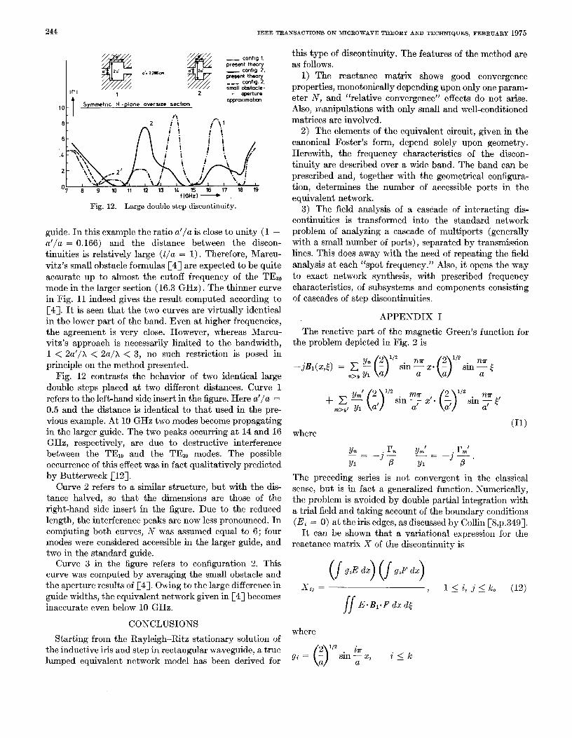
Fig. 12. Large double step discontinuity.

guide. Inthisexample theratio a’/aisclose tounity(l –

a’/a = 0.166) and the distance between the discon-

tinuities is relatively large (t/a = 1). Therefore, Marcu-

vitz’ssmall obstacle formulas [4]areexpected to be quite

accurate up to almost the cutoff frequency of the TEw

mode in the larger section (16.3 GHz). The thinner curve

in Fig. 11 indeed gives the result computed according to

[4]. It is seen that the two curves are virtually identical

in the lower part of the band. Even at higher frequencies,

the agreement is very close. However, whereas Marcu-

vitz’s approach is necessarily limited to the bandwidth,

1 < 2a’/~ < 2a/h <3, no such restriction is posed in

principle on the method presented.

Fig. 12 contrasts the behavior of two identical large

double steps placed at two different distances. Curve 1

refers to the left-hand side insert in the figure. Here a’/a =

0.5 and the distance is identical to that used in the pre-

vious example. At 10 GHz two modes become propagating

in the larger guide. The two peaks occurring at 14 and 16

GHz, respectively, are due to destructive interference

between the TEIO and the TESO modes. The possible

occurrence of this effect was in fact qualitatively predicted

by Butterweck [12].

Curve 2 refers to a similar structure, but with the dis-

tance halved, so that the dimensions are those of the

right-hand side insert in the figure. Due to the reduced

length, the interference peaks are now less pronounced. In

computing both curves, N was assumed equal to 6; four

modes were considered accessible in the larger guide, and

two in the standard guide.Curve 3 in the figure refers to configuration ~. This

curve was computed by averaging the small obstacle and

the aperture results of [4]. Owing to the large cliff erence in

guide widths, the equivalent network given in [4] becomes

inaccurate even below 10 GHz.

CONCLUSIONS

Starting from the Rayleigh-Ritz stationary solution of

the inductive iris and step in rectangular waveguide, a true

lumped equivalent network model has been derived for

this type of discontinuity. The features of the method are

as follows.

1) The reactance matrix shows good convergence

properties, monotonically depending upon only one param-

eter N, and (‘relative convergence)’ effects do not arise.

Also, manipulations with only small and well-conditioned

matrices are involved.

2) The elements of the equivalent circuit, given in the

canonical Foster’s form, depend solely upon geometry.

Herewith, the frequency characteristics of the discon-

tinuity are described over a wide band. The band can be

prescribed and, together with the geometrical configura-

tion, determines the number of accessible ports in the

equivalent network.

3) The field analysis of a cascade of interacting dis-

continuities is transformed into the standard network

problem of analyzing a cascade of multiports (generally

with a small number of ports), separated by transmission

lines. This does away with the need of repeating the field

analysis at each “spot frequency.” Also, it opens the way

to exact network synthesis, with prescribed frequency

characteristics, of subsystems and components consisting

of cascades of step discontinuities.

APPENDIX I

The reactive part of the magnetic Green’s function for

the problem depicted in Fig. Z is

(11)where

The preceding series is not convergent in the classical

sense, but is in fact a generalized function. Numerically,

the problem is avoided by double partial integration with

a trial field and taking account of the boundary conditions

(,?3, = O) at the iris edges, as discussed by Collin [8,P.349].

It can be shown that a variational expression for the

reactance matrix X of the discontinuity is

where

()2 1/2 ~T

gi= – sin — x, i<lca a

ROZZI Ah’D MIWKLEh’BRkUKI,:R: WIDE-BAND NETW”ORK MODELING

and13,F are ‘(trial fields.”

By carrying out double partial integration and upon

application of the boundary conditions at the iris edge, we

obtain

[!(d~/dX) hi {~~w

(dF/dx) hi dx1Xij = T{Tj ‘—--- ‘——-— (13)

JJ

where

{

cos (i7r/a) J = @i, i<?+

h,, =

cos (i7r/a’) J’ = t,, k+l~’i~li..

The quantities q, ~, and B are those defined in (1) ; r, is

defined in connection with (9). Using the matrix represen-

tation introduced in (~)-(7) it can be shown ~fi] that

(13) can be written as

which is formula (9) of Section II.

APP13~DIX H

Here we shall derive a recursive formula for the co-

efficients P.P of (3).

Consider the recursive formula for the Chebyshev poly-

nomials of the first kind:

T.(x) = 2X2’-,(X) – J!’._,(r) (111)

and set in the above

Cos ~ x = 1’. ()cm ~ d = ?’.(4 + 0!2 Cos 0). (11~)a a

lJsing the trigonometric identity,

Cosil. cospo = ; [cm (J) – 1)?9 + Cos (p + 1)81.

(111) becomes

245

k P.. Cos po = 2CY, “g’ P..,,p Cos pr9 – ‘~’ P._,,p cm pt?p=lr ~=o p=o

n—2

+ a, x F’n-l,p+l Cos P8 + @ 5 P.-l, p-l Cos po. (113)*=—1 ~=1

Considering coefficients of cos p8, yields

P.p = ,Z@n-l,p – P.–23P + Cz2p.-l,p+l

+ a2&,pPn-ur + cc2Pn_1,p-1 (H4)

where

1

0, p%l

81,P =

1, p=l

Pull = 1, Plo = al, I’ll = w

and

P.. = o, ifn<porp<O.

(114) is the sought recursive formula.

[1]

r2]

r3.]

[4]

[.5]

[61

[7]

[s]

[9]

[10]

[11]

[12]

REI~ERE~CES

1<. F. Harringtonl Field Cornputatzon by the J1ornerit hfetho<l.New York: Macmdlan, 1964.J. Schwinger and D. Saxon, Dis,continuities zn ~t~aueguides.New York: Gordon and Breach, 1968.T. Itoh and 1{. Mittra, “A method for solving bounddry valueproblems associated with a class of doubly modified Weiner–Hopf structures,” Proc. IEEE (Lett.), vol. .57, pp. 217&2171,I)ec. 1969.N. Marcuvitz, Waueguzdc Handbook (LI.I.T. Jladiation Labora-tory Series). New York: McGraw-Hill, 19.51.T. E. Rozzi, “Hilbert space approach for the analysis of multi-modal t iansmission lines and diseontinuities, ” in 1979 NA 1’0Sy~~lp. Network and Sigrwd Z’fworU (Bournernouth, England),J. Scanlan and J. Skwirzynski, Ed. London, England:Pere~rinlls. 1973.T. E; R oz;i, “Network analysis of strongly coupled transverseapertures in waveguide,” Int. J. circuit Theory Appl.j vol. 1,pp. 161-179, 1972.T. E. Rozzi and W. F. G. hfecklenbra~lker, “Field and networkanalysis of waveguide discontinuities, ” in Proc. 1973 EuropeanMicrowaue C’onf.. vol. 1. Paner B-l-2.R. Collinj Fierc~ Theory of G~ided W’ewes. New York: McGraw-Hill; 1960, ch. 8.T. E. .Rozzi, “The variational treatment of thick interactinginductive irises,” IEEE Trans. Microwate Theory Tech., vol.&ITT-21, pp. 82–88, Feb. 1973.D. S. Jones, The Theor~ of .Wectrornagnetism. New York:Pergamon, 1964, ch. 4.V. Belevitch, L’[assical Netu,ork Theory. San Francisco, Calif.:Holden-Day, 1968, ch. 8.II. J. Butterweck, “A theorem about lossless reciprocal three-ports,” IEEE Trans. Circuit Thror~ (Corresp.), vol. CT-I.5) pp.74–76, &lar. 1968.