wi - virginia tech · bankruptcy filing process and the legal aspects of deciding the disposition...
TRANSCRIPT
wiml ci
BANKRUPTCY OUTCOME AFTER
THE POINT OF FILING
byLarry Allen Lynch
Dissertation submitted to the Faculty of the
Virginia Polytechnic Institute and State University
in partial Fulfillment of the requirements For the degree 0F
Ph.D in Finance
in
Finance, Insurance and Business Law
APPROVED:
I\
ADanaJ. .yf1‘insogCha1rman
F / FF- F J7 «
A F .^ }•
Randall S. Billingsle37)
Arthur J. |Keown
„ ·F ·— L„
F.
Robert E. Lamy Q- L/ ° Gäoängy Thompson
FNovember 17, 1987
Blacksburg, Virginia
JgE
‘¤
SE EBANKRUPTCY OUTCOME AFTER
Ä, THE POINT OF FILING
äv
» byW
_ Larry Allen Lynch
Dana J. Johnson, Chairman
Finance, Insurance and Business Law
(ABSTRACT)
The subject of corporate bankruptcy has been of interest to financial academicians and
practitioners alike. Researchers have directed most of their attention to accounting‘
based models for predicting bankruptcy filings. Although some research has attempted
to estimate the probability and costs of bankruptcy, a very limited amount is centered
around the outcome of bankruptcy proceedings. Specifically, littleis known about the
circumstances that determine whether the firm will liquidate, successfully reorganize, or
become an acquisition of another firm after filing for court protection. Given the po--
tentially large losses to both creditors and stockholders, the determinants ofbankruptcy
outcome should be of considerable interest. The focus of this research is threefold.
First, the factors that should have an effect on the disposition of the firm after the
bankruptcy filing are exarnined for their influence on the disposition. Second, since there
is some dispute as to the appropriate classification of acquired firms, the correct classi-
fication of acquired (or merged) firms is determined. Third, the effect ofa major change
in the bankruptcy law is examined.
ii

Acknowledgements
There are so many people to whom I am indebted for their assistance, kindness, and
understanding during the long and arduous process of preparing this dissertation.
Without their support, this project would never have been completed.
&
To begin, I wish to thank my chairperson, Dr. Dana J. Johnson, who has provided me
· with much needed inspiration, advice, and encouragement throughout my studies.
· Without her I would never have made it. I also wish to thank the other members of
my committee, Dr. Authur Keown, Dr. G. Rodney Thompson, Dr. Randall Billingsley,
and Dr. Robert Lamy. Their guidance and assistance have been invaluable.
I must express my deepest appreciation to my colleagues in the Business Administration
and Economics department at Roanoke College. Their confidence and support during
my studies kept me going when the task seemed insurmountable.
Next, I wish to thank my family. My daughter, parents and sister have enjoyed precious
little of my time during the pursuit of this degree. Their understanding and support have
been very important to me and allowed me to focus my attention on the task at hand.
Acknowledgements 5;;

I love them all more than they know. I pledge to make up the time they have given up
for my degree pursuit.
Finally, I wish to thank my wife, , for her support, encouragement, tolerance, and
love as I completed the study. No one knows more than she how much time and effort
has gone into this work. lt is to her that I dedicate this dissertation.
Acknowledgementsiv
Table of ContentsChapter One: Introduction ...........................................1
Contribution .....................................................2Organization of Study ..............................................3
Chapter Two: Law and Literature Review ................................4I
Introduction..................................................‘....4z The Law
Claimholder Settlements ...........................................7Disposition of the Bankrupt Firm and the Filing Process ...................7
Background Literature Review .......................................10
Bankruptcy Prediction Models ......................................Il
Bankruptcy Costs ...............................................13
Disposition of the Firm in Bankruptcy .................................15
Chapter Three: Data, Model and Methodology ............................23
Introduction.....................................................23
Table of Contents V
Variable Selection.................................................23
Ownership Concentration (OWN) ...................................24
Liquidity (LIQ) .................................................25u
Bank Debt (BANK) .............................................26
Tax Loss Carryovers (TAX) .......................................26
Free Assets (FA) ................................................27
Earnings Prospects (ROA) .........................................28
Size (SIZE) ....................................................28
Return Variance (VAR)...........................................29
Return Skewness (SKEW) .........................................29
Coupon Rate (COUP) ............................................30
/Bankruptcy Law (LAW) ..........................................31
Sample .........................................................31
Missing Data ....................................................33
· · Outcome Estimation Model .........................................35
Effect of the Law Change ...........................................43
Chapter Four: Results .............................................45
Introduction .....................................................45
Categorization of Acquired Firms .....................................46
Acquired Versus Liquidated ........................................46
Acquired Versus Reorganized ......................................53
Reorganized versus Liquidated .......................................58
Continued versus Liquidated .........................................65
Effect of the Law Change ...........................................66
Table of Contents vi
Chapter Five: Summary and Directions for Future Research ..................76U
Introduction.....................................................76
Summary .......................................................77
Limitations and Future Research .....................................79
Bibliography .....................................................80
Appendix A. List of Firms in Study ....................................83
Appendix B. Logit Analyses with Overall Average lmputation .................87
Vita .......................................................I....92
Table of Contents vii
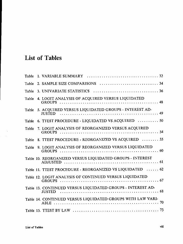
List of Tables
Table 1. VARIABLE SUMMARY ..................................32
Table 2. SAMPLE SIZE COMPARISONS ............................34
Table 3. UNIVARIATE STATISTICS ...............................36
Table 4. LOGIT ANALYSIS OF ACQUIRED VERSUS LIQUIDATEDGROUPS ...............................................48
Table 5. ACQUIRED VERSUS LIQUIDATED GROUPS - INTEREST AD-JUSTED ...............................................49
Table 6. TTEST PROCEDURE - LIQUIDATED VS ACQUIRED ..........50
Table 7. LOGIT ANALYSIS OF REORGANIZED VERSUS ACQUIRED° GROUPS ...............................................54
Table 8. TTEST PROCEDURE - REORGANIZED VS ACQUIRED ........55
Table 9. LOGIT ANALYSIS OF REORGANIZED VERSUS LIQUIDATEDGROUPS ...............................................60
Table 10. REORGANIZED VERSUS LIQUIDATED GROUPS - INTERESTADJUSTED .............................................61
Table 11. TTEST PROCEDURE - REORGANIZED VS LIQUIDATED ......62
Table 12. LOGIT ANALYSIS OF CONTINUED VERSUS LIQUIDATEDGROUPS ...............................................67
Table 13. CONTINUED VERSUS LIQUIDATED GROUPS - INTEREST AD-J USTED ...............................................68
Table 14. CONTINUED VERSUS LIQUIDATED GROUPS WITH LAW VARI-ABLE ..................................................70
Table 15. TTEST BY LAW .........................................73
List of Tables viii
Chapter One: Introduction
The subject of corporate bankruptcy has been of interest to financial academicians and
practitioners alike. Researchers have directed most of their attention to accounting
based models for predicting bankruptcy filings. Although some research has attempted
to estimate the probability and costs of bankruptcy, a very limited amount is centered
_ around the outcome of bankruptcy proceedings. Specifically, little is known about the
circumstances that determine whether the firm will liquidate, successfully reorganize, or
become an acquisition of another firm after filing for court protection. Given the po-
tentially large losses to both creditors and stockholders, the determinants ofbankruptcy
outcome should be of considerable interest. The focus of this research is threefold.
First, the factors that should have an effect on the disposition of the firm after the
bankruptcy filing are examined for their influence on the disposition. Second, since there
is some dispute as to the appropriate classification of acquired firms, the correct classi-
fication of acquired (or merged) firms is determined. Third, the effect of a major change
in the bankruptcy law is examined.
Chapter Onc: Introduction I
Corztribution
Financial theory dictates that liquidation should occur if the market value of the
firm is less than the liquidation value. In practice, however, numerous aspects affect the
actual outcome of a bankruptcy firm. First, the market value of the firm is used in fi-
nancial theories, but courts often use book value to settle priority claims. Second,
management may be acting in their own self-interest since their own value in the labor
market may be affected. Third, there may be agency costs of renegotiating debt con-
tracts. As an example, unsecured debt may be renegotiated for secured debt. This re-
structuring of debt may affect the preference of some claimants on the firm as to the
outcome of a bankruptcy filing. Fourth, the interpretation and application of bank—
ruptcy laws often favor a certain class of creditor and allow for the possible breakdown
of the priorities of claims. The fates of stockholders and creditors of firms in financial
q distress are often not under their own control and, further, differ with respect to the
disposition of the firms.i
As stated above, the purpose of this study is threefold. First, the factors relating
to the disposition of firms from the point of filing for legal bankruptcy are examined.
Then using variables hypothesized by prior theories, a model is developed to estimate the
likelihood of bankruptcy outcomes in terms of liquidation versus continuation given the
announcement of filing. Next, the empirical question of whether the acquired firms
should be grouped with the liquidated firms or with the reorganized (continued) firms is
investigated. White (1983) groups acquired firms with liquidated firms. Casey, et. al.
(1986) remove acquired firms from their sample. Since the effect on the various claim-
ants of the liquidated firm is generally different from that of the acquired firm, the
Chapter One: introduction 2
grouping of the two outcomes is questionable. The model will be tested to determine the-
appropriate grouping. Finally, the 1978 Reform Act is exarnined to test for structural
changes in several variables as well as the overall model.
Organization of Study
Since the bankruptcy law plays a major role regarding the disposition of the firm
after filing, it is discussed at length in the next chapter. This discussion is in two parts:
the law that existed prior to 1979 (hereafter the pre-1979 law) and the Reform Act of
1978 (hereafter the Reform Act) which was implemented on October 1, 1979 and re-
mains in effect today. The second chapter also presents a review of the literature.
The third chapter presents details of the research methodology including a de-
· scription of the logit model and the selection of variables. The results of the study are
presented in chapter four, including tl1e grouping of the acquired firms and the effect of
the law change. The fifth and final chapter presents a summary of the results and rec-
ommendations for further research.
Chapter One: Introduction 3
Chapter Two: Law and Literature Review
IIlII'0dllCIi0ll .
The purpose of this chapter is to review the bankruptcy laws as they existed before
. the 1978 Reform Act as well as after the Act was passed. Also, this chapter will review
the literature dealing with bankruptcy. The law is discussed with emphasis on pertinent
changes that occurred with the Reform Act. The bankruptcy literature is reviewed
looking first at background studies, then reviewing the prediction models. Next, litera-
ture on the costs of bankruptcy is discussed. Finally, literature on the disposition of the
firm is reviewed.
Chapter Two: Law and Literature Review 4
Tha Law
The purpose of this section is to discuss the pre-1979 law and the changes made to
it by the 1978 Reform Act (as stated above, the law went into effect in 1979). The ap-
proach used for this comparison is to discuss each of the following in turn: a brief his-
tory of bankruptcy law; the order of priority of claimholder settlement; and the actual
bankruptcy filing process and the legal aspects of deciding the disposition of the firm
after filing.
The Bankruptcy Reform Act of 1978 replaced the Bankruptcy Act of 1898. Al-
though there was a flurry of emergency legislation passed during the early 1930’s, in re-
sponse to the depression of 1929, the 1898 law remained basically unchanged until the
Chandler Act of 1938. The Chandler Act amended the 1898 law to deal with the finan-
cial crises of the depression era but did not completely modernize the Act of 1898. Two
chapters of the Chandler Act were closely related to corporate bankruptcy and reor-
ganization attempts. Chapter XI proceedings were voluntary and applied only to unse-
cured creditors. Chapter X proceedings could be voluntary or involuntary and were
more restrictive than Chapter XI proceedings. Chapter XI was generally preferred by
the debtor since Chapter X automatically placed an outside trustee in control of the firm
during the bankruptcy proceeding.
ln 1970 Congress formed the Commission on the Bankruptcy Laws of the United
States to study and recommend changes to bring the entire bankruptcy system up to
date. The end product of the Comrnission's work was the Bankruptcy Reform Act of
Chapter Two: Law and Literature Review 5
1978. The change in bankruptcy laws is important to the present study since it could
have a significant impact on the disposition of a troubled firm.
H. R. Miller and M. L. Cook in their "A Practical Guide to the Bankruptcy Reform
Act," found the following to be among the most significant changes brought about by
the Reform Act of 1978 affecting corporate bankruptcies:
a. The Bankruptcy Court’s increased independence and full
jurisdiction.
b. Appointment of the bankruptcy judges by the President for
14-year terms.
c. The United States trustee pilot program.
d. The consolidation of Chapters X, XI and XII into a single
reorganization Chapter 11. (The Reform Act dropped thel
pre-1979 law’s Roman numeral designation).
e. The simplification of the test for involuntary petitions.
fi A simplification of the bankruptcy trustee's statutory
avoiding powers.
g. Expedited hearings on relief from stay and provisions to
safeguard collateral.
Chapter Two: Law and Literature Review 6
Claimholder Settlements_
Since claimants on the firm have specific rights under law which might affect the
outcome of a bankruptcy filing, it is important to review how claimholder setelements
are made. First, the secured creditors may reclaim their principal and interest from the
specific assets against which they have a lien. lf their claims exceed the value of their
security, they become unsecured creditors for thesbalance. The balance of the assets are
disposed of by the trustee and the proceeds from this disposition are paid out according
to the absolute priority rule. Highest in priority is the cost of administering the bank-
ruptcy, including lawyers’ fees and other expenses incurred after the filing for bank-
ruptcy. Second in priority are creditors’ claims arising, in an involuntary case, in the
ordinary course of business after the petition is filed. Wage claims up to a limit of $2000
($600 under the old Act) are granted third priority. Certain fringe benefits are given
fourth priority. The fifth priority in the new law is for consumer creditors who have paid
q money in connection with the purchase or rental of property or the purchase of services
which have not been delivered. Any taxes owed occupy the next priority provided by
both acts. Seventh on the priority list are the unsecured creditors such as trade creditors,
bondholders and banks. Preferred stockholders are eighth and, finally, the common eq-
uity holders receive the balance of the proceeds.
Disposition of the Bankrupt Firm and the Filing Process
The three potential outcomes a financially distressed corporate entity faces are liq-
uidation, reorganization under court protection, and acquisition by another firm. When
Chapter Two: Law and Literature Review 7
a firm files for liquidation, a trustee is appointed by the court to oversee the liquidation
of the assets.
Reorganization under the old Bankruptcy Act allowed failing firms to file for pro-
tection through the court while continuing to operate without substantial change in form
or management. Management would propose a settlement with creditors which specified
a cutback in unsecured debt claims and secured creditors were prevented from foreclos-
ing on their lien assets. The plan had to be approved by majority vote of all unsecured
creditor classes. Since only the managers had a right to propose a plan, the creditors’
had little alternative to accepting the plan. If the plan was not accepted, then liquidation
followed.
The new Bankruptcy Reform Act stiffened the voting requirements by stating that
a two-thirds majority in each class must vote in favor of a plan. The new law also re-
quires that secured as well as unsecured creditor classes approve the plan if their claims
are adversely affected. However, the managers no longer have the exclusive right to
propose a plan. Creditors now have other alternatives to either liquidation or the man-
agers’ plan. If no plan is accepted, the firm can continue to operate while a buyer is
sought. Finally, the new Reform Act removed the restriction that firms reorganizing
must continue in the same form, meaning that parts of the firm may be sold or elirni-
nated.
The old Act generally required that a trustee be appointed if the filing was under
Chapter X, and did not permit the appointment of a trustee in a Chapter XI case. This
situation caused debtors to favor filing under Chapter XI since they did not want to be
restrained in the management of the business. In consolidating the chapters, the Reform
Act adopted the flexible approach of leaving the debtor in control of the business unless
Chapter Two: Law and Literature Review 8

a request is made for the appointment of a trustee. Should this occur, a court hearing-
is held to determine the need for a trustee.
There are now three basic ways of cornmencing a bankruptcy case where a corpo-
ration is concerned. A voluntary case begins with the filing of a petition by the man-
agement of the firm. Involuntary cases may be filed under the liquidation provisions of
Chapter 7 or the reorganization provisions of Chapter 11 of the Reform Act, but an in-
voluntary petition may be filed only if the debtor is generally not paying its debts or a
custodian has been appointed for the debtors property. An involuntary petition may
be filed by three or more creditors having claims aggregating at least $5,000 more than
the value of any lien securing such claims, unless there are fewer than twelve creditors.
In that case, one or more creditors holding claims of at least $5,000 may file. The Re-
form Act specifically provides that an indenture trustee may be a petitioning creditor.
A case ancillary to a foreign proceeding is commenced by the filing ofa petition with theI
bankruptcy court by a foreign representative. ·
The new bankruptcy laws contained in the Reform Act were generally effective on
October 1, 1979. However, the new bankruptcy court system did not take effect until
April 1, 1984. The full effect of the changes in the law may not be evident in empirical
research prior to the new court system being in place.
Chapter Two: Law and Literature Review 9
Background Literature Review
A number of issues have been dcalt with in the literature concerning bankruptcy,
its costs and its probability of occurrence. These issues are of importance due to their
hypothesized effect on the question of cost of debt and equity financing and the exist-
ence of an optimal capital structure. The capital structure literature generally centers
on the trade—off between the tax advantages of debt financing and the expected costs of
bankruptcy. The existence of an optimal capital structure has been modeled in numer-
ous studies, including those by Kraus and Litzenberger (1973), Kim (1976), Scott (1976),
and DeAngelo and Masulis (1980).
Given the important role of capital structure in the development of financial the-
ory, a considerable amount of research has been undertaken in the bankruptcy area. It
has traditionally focused on measuring the costs of bankruptcy or estimating the prob-l
ability of bankruptcy, often through a group of models classified as bankruptcy predic-
tion models. Until recently, little attention had been directed at the importance of the
definition of bankruptcy. More specifically, recent studies have recognized that while
the law permits a bankruptcy filing, this action does not mean that the firm will liquidate
or cease to exist. After filing, the bankruptcy law permits the firm to follow one of the
three avenues; liquidation, reorganization, or acquisition by another firm. Each of these
outcomes has its own implications for the debtholders and stockholders of the firm.
In this section, the literature pertaining to the aforementioned areas of prior re-
search - bankruptcy prediction, cost measurement, and disposition of the firm after
filing - are examined.
Chapter Two: Law and Literature Review 10
Bankruptcy Prediction Models
Early work examining the probability of bankruptcy centers on the use of financial
ratios and various regression techniques. Beaver( 1967) is among the earliest works to
study failure prediction. He analyzes 79 firms that failed between 1954 and 1964 along
with a paired sample of non·failed firms and, using a univariate approach, he tests the
usefulness of ratio analysis for predicting bankruptcy. Beaver concludes that it is pos-
sible for accounting data to predict failure five years in advance. His testsiof 30 ratios
(using dichotomous classification tests and analysis of likelihood ratios) finds cash flow
to total debt to be the key variable.
Altman (1968) uses multiple discriminant analysis of 66 firms to arrive ata five
variable linear model for bankruptcy prediction consisting of (1) working capital/total
assets, (2) retained earnings to total assets, (3) EBIT/total assets, (4) market value of
equity/book value of total debt, and (5) sales/total assets. This model, however, does
not have predictive ability beyond two years prior to failure. Deakin (1972) develops
an alternative to the Beaver and Altman models. He utilizes linear multiple discriminant
analysis to modify A1tman’s model to include Beaver’s fourteen best predictors and ob-
tains a combination of ratios which yields predictive accuracy three years in advance of
failure. The sample size is 32 firms that failed between 1964 and 1970 and a paired
sample of non- failed firms.
Chapter Two: Law and Literature Review ii
Altman, et.al. (1977) employ both linear and quadratic classification equations to
arrive at a seven variable "ZETA" model consisting of (1) return of assets, (2) stability
of earnings, (3) debt service, (4) cumulative profitability, (5) liquidity, (6) capitalization,
and (7) size. Their sample consists of 53 bankrupt firms and a matched sample of non-
bankrupt firms. The ZETA model outperforms Altman’s earlier model. Dambolena and
Khoury (1980) also use financial ratios and discriminant analysis in their stability model.
They employ a sample of 46 firms to introduce various measures of ratio stability to
improve the predictions, relative to those of Altman’s.
Wilcox (1976) analyzes 52 failed and 52 non-failed firms to demonstrate that tech-
niques based on ratios are poor predictors for periods longer than one year. This is be-
cause ratios vary across industries and across time and that they are easily "window
dressed" by managers. He presents a technique based on the gambler's ruin approach
and provides evidence of its superiority for periods longer than one year to failure.
Vinso (1979) criticizes the ratio based models as being static in nature. He also criticizes
models based on first passage of time techniques since they rely on the assumption that
ruin is eventually a certainty. Building on Wilcox, he presents his dynamic "risk 0fruin"
technique as being "consistent with or superior to other risk measures currently avail-
able."
Citing the limited information in ratio and earnings data, Ahrony, Jones and Swary
(1980) suggest an approach to estimate the probability of failure based on a company’s
market rates of return. With a sample of 45 failed industrials and a group of 65 control
firms, they develop a model which compares favorably with ratio based models.
Chapter Two: Law and Literature Review 12
The studies reviewed above demonstrate an academic interest in the bankruptcy-
question and the outcome of firms in financial distress. The next section reviews the
literature pertaining to the costs associated linancially distressed firms.
Bankruptcy Costs
The second area of concern is the identification and measurement of" the costs of
bankruptcy. The literature refers to both direct and indirect costs of bankruptcy. Gen-
erally, direct costs are the legal and administrative costs associated with the process of
filing and executing a bankruptcy. lndirect costs include implicit costs such as loss of
profits caused by the loss of sales.
Some have argued that bankruptcy costs are insignificant to the theory of optimal
capital structure. The first major attempt to measure bankruptcy costs was undertaken
by Warner (1977). Whether his study could be generalized to include other industries
is questionable since he investigates only ll rail earriers over the 1933 to 1955 time pe-
riod. He demonstrates with his sample of railroad bankruptcies that direct bankruptcy
costs are on average only one percent of a firm’s market value prior to bankruptcy.
Others also suggest that bankruptcy costs are not of importance to capital Struc-
ture. Miller (1977) refers to Warner’s study and argues that, in a world of difTerentia1
personal taxes, the marginal personal tax disadvantage ofdebt combined with the supply
side adjustments by firms will override the corporate tax advantage of debt, driving
market prices to equilibrium implying capital structure irrelevance to any given firm.
Haugen and Senbet (1978) conclude that, if capital market prices are determined by ra-
Chapter Two: Law and Literature Review 13
tional investors, informal reorganization would occur making bankruptcy costs trivial
or nonexistent.
White (1983) distinguishes between ex-ante and ex-post bankruptcy costs. She
defines ex-ante bankruptcy costs as an agency cost, where managers do not act in the
interest of the stockholders but in their own self-interest, trying to keep a firm operating
when it should be liquidated. The ex-ante cost is the difference between the net liqui-
dation value of the firm and the present value of the future income stream given con-
tinuation or reorganization. This definition of ex-ante costs is similar to the indirect
costs referred to in other studies. White considers the direct bankruptcy transaction
costs as ex-post costs. Titrnan (1983) also discusses the capital structure problem from
the standpoint of bankruptcy costs arriving from the agency relationship. He investi-
gates the relationship between the firm (as the agent) and its customers (as principals)
who suffer costs if the firm liquidates.
. Altman (1984) considers indirect costs as well as direct costs and presents two
proxies for measuring these costs for 12 retailers and 7 industrial firms. The first proxy
he uses is a regression of firm sales on the appropriate industry sales figure for a ten year
period prior to the forecasted year. Next he uses the estimates of security analysts to
determine lost profits. He finds that total bankruptcy costs (direct plus indirect), on
average, range from 12.4% three years prior to bankruptcy to 16.4% just prior to
bankruptcy.
Noting the measurement problems of previous studies, Kalaba, Langetieg,
Rasakhoo, and Weinstein (1984) demonstrate with a simulation that quasilinear esti-
mation is a potentially reliable and efficient technique for the estimation of implicit
bankruptcy costs. An empirical study remains to be done for validating their contention.
Chapter Two: Law and Literature Review 14
The above research demonstrates that much concern exists over the outcome of theV
financially distressed firm due to the potentially large costs of bankruptcy. With the
exception of Michelle White’s work, most of these models have treated bankruptcy as a
generic concept, ignoring the different outcomes and the different costs. The next sec-
tion reviews literature dealing directly with the disposition of firms in financial distress.
Disposition of the Firm in Bankruptcy
A central concern of this study is the disposition of a firm after it files for bank-
ruptcy. The concept of bankruptcy and the financially distressed firm is currently gain-L
ing the interest of many academicians, however the definition of bankruptcy is an
unclear issue. Is a firm considered bankrupt when it cannot meet the current payment
on its debt obligations, when it violates indenture provisions or is it bankrupt when it
actually files for protection under the court system? Is a firm bankrupt only when it
liquidates or is it considered bankrupt while it is undergoing reorganization? Jensen and
Meckling (1976) argue that bankruptcy and liquidation are different events and that
liquidation will occur only if the market value of future cash flows generated by the firm
is less than the market value of the assets if they were sold piecemeal.
Warner (1977) uses the term, bankruptcy, to refer "to proceedings which are
undertaken under bankruptcy laws when a corporation is unable to pay or reach agree-
ment with its creditors outside of court". Once a firm files for protection under the
courts, the claimants on the firm are subject to outcomes different from those they bar-
Chapter Two: Law and Literature Review 15
gained for when purchasing their respective securities. Warner further points out that
courts typically do not follow the priorities of securities’ claims in bankruptcy pro-
ceedings making the determination ofthe outcome ofa court proceeding ofgreat interest
to the claimants.
Recent studies have become concerned with the alternatives available under actual
bankruptcy proceedings. White (1983) considers the three options of liquidation, con-
tinuation, and reorganization and discusses the tendency ofmanagement to continue the
firm even when liquidation may be more appropriate. She argues that since managers
not wanting to be displaced have an incentive to resist liquidation as long as possible,
the bankruptcy reorganization process prolongs the continuation of inefficient firms.
This offsets the beneficial effects of competition, and efficiency can be improved by re-
ducing the likelihood of reorganization. She maintains that the new Bankruptcy Code
does just that. She also discusses the shift from unsecured to secured debt by failing
’ ‘ firms delaying bankruptcy. This action perrnits the proportion of debt financing to in-
crease and leads to a breakdown in the "me-first" priority rules associated with Fama and
Miller and in the order of claims covered by the Bankruptcy Code. White uses a sample
of 186 firms in the Southern District of New York which liquidated or reorganized in
1978-1979 and a sample of 121 firms from 1980.
Baldwin and Mason (1983) use an options pricing framework to formulate recon-
tracting of debt and equity such that absolute priority rules do not hold. They found
that, in the case of the Massey Ferguson Ltd. reorganization, absolute priority rules did
not hold and that the market expects debt and equity claims to be recontracted before
equity is eradicated.
Chapter Two: Law and Literature Review I6
Lewellen (1971) brings mergers into the bankruptcy argument by arguing that for_
mergers to be beneficial, a merger must reduce the probability of one of the firms in-
volved defaulting on its debt. Should this occur, the debt should increase in value
making the merger beneficial. Further consideration of the merger outcome is supported
by Kim (1978) when he states "...in order for the bankrupt firm to receive even a fraction
of tax credits for its losses, either the firm must merge with a profitable firm or it must
carry·forward its tax losses after the bankruptcy.? Scott (1977) notes a similar tax ben-
efit in the acquisition of the financially distressed firm, but also notes that the relative
size of the acquirer and the target are important. Shrieves and Stevens (1979) present
empirical evidence of mergers occurring for the purpose of avoiding bankruptcy. They
use a sample of 112 acquircd and 112 nonacquired firms and Altman's Z score model to
argue a bankruptcy avoidance rationale for mergers.
Clark and Weinstein (1983) recognize that investors do not expect the firm to liq-
uidate as a result of filing for bankruptcy. They use daily and monthly price and return1
data on 138 firms petitioning for reorganization during the period between 1938 and
1979 in order to investigate the "Bankruptcy Announcement Effect" around the filing
date. They conclude that bankruptcy filings convey important unanticipated informa-
tion to the market. They also check for different behavior under Chapter X and Chapter
XI of the old Act. Their findings offer limited support for the proposition that a Chapter
X filing, which generally took control away from existing management, was worse news
for shareholders than a Chapter X1 filing. However, they drew no conclusion due to
small samples.
Bulow and Shoven (1978) describe a model with three classes of claimants on the
income and assets of the firm, specificallyz
Chapter Two: Law and Literature Review 17

a. bondholders - a non-cohesive group with a fixed time
pattern of claims.
b. bank lendcrs - with loans due each period; they have
ability to negotiate with equity holders.
c. equity holders - residual claimants who always wish to
avoid bankruptcy.
Bulow and Shoven treat bank lenders and equity holders as a coalition with the
bank lender holding the decision making power as to whether the firm willicontinue or
liquidate. They develop a two—period model where bankruptcy occurs when the two
negotiating claimants, the bank and the equity holders, have a more valuable joint claim
„ . under liquidation than with continuance. Also, bankruptcy will occur if bankruptcy
cost, defined as the difference between the value as an ongoing concern and the liqui-
dation value, is less than the value of bondholders' claims under continuance minus the
value ofbondho1ders’ claims under liquidation. Initial financial crisis can be represented
by a negative net worth condition, or when there is insufficient cash to pay all current
claims.
If continuation is to occur then the additional funds needed are optimally obtained
from the bank if the difference between the value of the firm under continuance minus
the liquidation value is less than the value to debtholders under continuance minus the
value to debtholders under liquidation.
Chapter Two: Law and Literature Review l8
Bulow and Shoven present numcrical examples to demonstrate the following re-l
sults:
A. A firm may stay in business dcspite having both negative
net worth and a cash shortage.
B. A firm may liquidate even when the going concern value
exceeds the liquidation value. s
C. A firm may stay in business even when its liquidation value
exceeds its going concern value.
D. If two firms have identical bankruptcy costs, variance of
returns, liabilities, and asset value, it is possible that
the firm with more cash will stay in business while the
other will not.
T E. It is possible that a lower liquidation value will improve
the position of bondholders by encouraging the bank to keep
the firm operating.u
F. Given liquidation value, higher present value of future
earnings may mean a less valuable bondholder claim.
G. Bond debt may receive a higher or lower payoff than bank
debt.
These results indicate that the outcome of a bankruptcy filing is not necessarily intuitive
and that more research is needed in the area.
Finally, they point out that the addition of tax considerations may change the
outcome of the firm’s bankruptcy decision and opens the possibility that a merger will
Chapter Two: Law und Literature Review F9
occur. Since the tax system allows losses to be accumulated and applied to future
earnings, the firm with losses has something of value which is lost in liquidation.
Therefore, the tax system may support the continuance of a firm or merger with another
firm and discouragc liquidation.
White (1980) extends the work of Bulow and Shoven. In her article she analyzes
the bankruptcy liquidation rules from a public policy standpoint. She defines the social
condition for continuance to be P > L or that the firm’s expected present value of future
earnings is greater than the liquidation value of its assets. She concludes that neither
absolute priority, proportionate priority nor the "me-first" rules leads to private invest-
ment incentives which are socially efficient except under a very restrictive set of as-
sumptions: bondholders must be paid the same amount regardless of whether the firm
liquidates or continues and all interest rates on bonds, both old and new, must be the
same as the current discount rate. The latter assumption is not likely to occur and the
first assumption is describing riskless debt which negates the concern of the bankruptcy
question entirely.‘
Golbe (1981) also uses the model of Bulow and Shoven to demonstrate that, al-
though equity holders may be risk neutral or risk averse with respect to their own re-
turns, they may be risk preferring with regard to firm returns, especially if the firm is in
financial crisis. He shows that increased variance does not increase the risk to equity
holders since their downside return is limited to loss of their investment if bankruptcy
occurs but their upside is not limited. Thus, increased variance increases the equity
holders' expected returns but not their risk. Debt holders, on the other hand, do not
share in the upside gain but do participate with the equity holders and the bank in the
downside risk. Therefore, a mean-preserving increase in the variance of the firm’s re-
Chapter Two: Law and Literature Review 20

turns increases the expectations of the equity holders at the expense of the bond holders._
Assuming the Bulow and Shoven coalition theory, this renders bankruptcy less likely.
While some work is being done in the area of bankruptcy dcaling with aspects of
the issue of continuation versus liquidation, little empirical research has been undertaken
in examining the factors which distinguish among outcomes of bankruptcies after filing
has occurred. Casey, McGee, and Stickney (1986) develop a multivariate model to dis-
tinguish between reorganized and liquidated firms with the variables motivated by
White’s work. They use probit analysis to empirically test their model and find that two
factors posited by White have discriminating power. They are the free assets percentage
and the earnings prospects of the firm. Their model is able to classify accurately in only
69% of the cases in their estimation sample and this drops to 59% for their holdout
sample.
There are major weaknesses in their study, however. First, they distinguish be-
tween reorganized and liquidated firms but ignore firms that are acquired. Many firms
that file for protection in the courts have intangible or conditional assets that may be
lost should liquidation occur. For example, tax loss carryovers are valuable to a reor-
ganized firm once it turns profitable or may be valuable to a profitable acquiring firm
immediately. The value of the tax loss carryovers are lost if the firm is liquidated.
Casey, McGee, and Stickney's model might have been more significant had they in-
cluded acquired firms along with reorganized firms in a single group called continued
firms.
Second, they limit ”predictor” variables only to those motivated by White. White’s
model is built using Bulow and Shoven as is Golbe’s, but variables with strong theore-
tical and intuitive significance are not present in the Casey, McGee, and Stickney model.
Chapter Two: Law and Literature Review 21
For example, the liquidity of the firm has theoretical support in Bulow and Shoven’s
Work and is intuitively appealing but was not considered in the Casey, McGee, and
Stickney model. The same holds true for tax loss carryovers. Bulow and Shoven pro-
pose that the amount of funds supplied by banklenders should have an effect on the
outcome. They are not clear as to whether the term "banklender” refcrs strictly to banks
or, more broadly, to private debt. In either case, the variable is not considered by Casey,
McGee and, Stickney. The variance of the firm’s returns is suggested by Golbe as af-
fecting the outcome of a financially distressed firm. including these variables should add
explanatory value to a multivariate model.
Third, when a firm’s plan is confirmed, it is out of bankruptcy. Should it fail again,
this constitutes another failure. Casey, McGee, and Stickney require three years of
continued "success" and this unnecessarily limits their sample. Finally, their holdout
group spans the change in the law. Based on White’s findings, the new Code should
have an effect on their variables. This study uses variables motivated by these recent
studies to investigate their influence on the outcome of the financially distressed firm
after they file for protection under the existing bankruptcy laws.
This chapter provides a review of the law and the literature pertinent to this study.
The next chapter provides a description of the statistical details and the research design.
Chapter Two: Law and Literature Review 22

Chapter Three: Data, Model and Methodology
Introduction
This chapter provides a description of the model and the statistical methods used
in this study. The first section introduces the variables selected for the study and their
proxies. Next, the sample is described. The third section describes the logit outcome
estimation model. Finally, the model to determine the effect of the law change is pre-
sentcd.
Variable Selection
The theoretical determinants of the outcome of a bankruptcy filing which are
operationalized in the present study are (1) Ownership Concentration, (2) Liquidity, (3)
Chapter Three: Data, Model and Methodology 23

Bank Debt, (4) Tax Loss Carryovers, (5) Free Assets, (6) Earnings Prospects, (7) Size,
(8) Return Variance, (9) Return Skewness, (10) Coupon Rate, and (1 1) Bankruptcy Law.
Each of these are discussed next.
Ownership Concentration (OWN)
The ability of the firm’s owners to affect management’s commitment to maintain-
ing the firm as an ongoing concern should have a direct effect on the outcome of the
firm’s bankruptcy proceeding. White (1983) introduces management commitment by
discussing the desire of the existing management to continue the firm in order to protect
their jobs. Management often has a substantial portion of their personal wealth in the
firm. If the firm does poorly and may go bankrupt, the manager’s irnmediate market
value will be adversely effected. They may lose their jobs as well as any wealth invested
in the firm. Jensen and Meckling (1976) argue that the manager is a utility maximizer
with both pecuniary returns and non-pecuniary returns (perquisites) of his employment
determining utility. As the manager’s share of equity declines, his propensity for
perquisite consumption increases. This characterizes the agency conflict between the
owner-manager and outside stockholders.
If the stock of a firm is closely held, i.e. if a few stockholders hold a substantial
number of shares, these stockholders may exert pressure on the management for the firm
to continue. If existing management has a substantial percentage ownership in the firm,
or is influenced by a concentration of ownership, continuation is expected as this
Chapter Three: Data, Model and Merhedeiegy 24
owner-management entity tries to keep secure its position and to prevent losses incurredA
in liquidation.
The eH‘ect of ownership concentration would be affected by the fact that the ability
to control the reorganization process is changed by the new Code. Management no
longer has the exclusive right to present a plan of reorganization. Creditors and/or other
interested parties may now present to the court alternative plans and the court chooses
the one which it determines to best provide f“or the various claimants on the firm. Thus,
one would expect the change in the bankruptcy laws to reduce the significance of the
ownership concentration variable.
The average number of shares held per stockholder serves as proxy for the con-
centration of ownership. This variable was the most diflicult to obtain for the sample
firms. Of the 101 firms in the sample, this variable is missing in 18 of the observations.
Liquidity (LIQ)
The higher the liquidity of the firm, the more likely it will not be liquidated. Re-
ferring to Bulow and Shoven (1980), the higher the liquidity, the lower the amount the —
banklender must put up to continue the firm. The likelihood of continuance should in-
crease with increased liquidity. The current ratio of the firm is used as proxy for
liquidity.
Chapter Three: Data, Modcl and Methodology 25
Bank Debt (BANK)
Bulow and Shoven’s coalition theory provides a strong argument for the inclusion
of the level of bank debt in any model predicting bankruptcy outcome. If banklenders
are willing to lend money to a firm in financial distress, they anticipate that the firm is
to fare better in the future. This would indicate that the firm is expected to continue.
Since banklenders often have security for their loans and thus have had limited voting
rights under the old Act, the change in the voting requirements requiring two-thirds
majority in each class should affect their ability to control the firm as predicted by Bulow
and Shoven. The proxy for bank debt will be the ratio of short- term borrowings of the
firm to the total debt.
Tax Loss Carryovers (TAX) q
Bulow and Shoven further point out that the addition of tax considerations may
change the outcome of the firm's bankruptcy decision. Since the tax system allows
losses to be accumulated and applied to future earnings, the firm with accumulated
losses has something of value that will be lost in liquidation. Therefore, "the tax system
may encourage continuance or merger and discourage bankruptcy." White (1983) con-
siders acquired firms in the same class as liquidated firms. Casey, McGee, and Stickney
(1986) ignore these firms altogether. lt is the contention of the present study that ac-
quired firms are part of the continued class. This concept is supported by the new
bankruptcy code which states that a firm does not have to continue in the same form.
The greater the amount of tax loss benefits available to an acquiring firm, the more
Chapter Three: Data, Model and Mexhedorogy 26

attractive an acquisition becomes. The accumulated tax losscs, in effect, become aA
contingent asset of the financially distressed firm. One would expect to see a positive
relationship between this variable and the continuance outcome. If no tax loss
earryovers are given on Compustat or listed in the Moody’s Industrial Manual, it is as-
sumed that none exist.
Free Assets (FA)
The more free assets a firm has, the greater the assets available for collateral for
further borrowing. White (1983) demonstrates analytically that assets not secured by
previous borrowing give the firm additional borrowing capacity to obtain funds to
emerge from financial distress. Casey, McGee, and Stickney (1986) find free assets to
be a significant discriminatory factor. Thus, firms with a high level of free assets should
show a tendency for continuation. However, the more secured debt the firm has, the
fewer the assets available for distribution to unsecured creditors. This should result in
a tendency for continuation since the unsecured creditors may fare better, and they, by
law, have the voting power to accept a plan for continuance. The theoretical arguments
represented by these two variables are in conflict and the effects may be offsetting. The
Casey, et.al. study used non-collateralized tangible assets divided by total tangible assets
as the proxy for the free asset variable. However, since senior debt may be secured by
general claims on assets, this study uses the ratio of total assets less total borrowings to
total assets as proxy for free assets. Total borrowings is available for all but one of the
observations.
Chapter Three: Data, Model and Methodology 27
Eamings Prospects (ROA)
White (1983) also introduces the idea that the more attractive the firm’s earnings
prospects in the near future, the more likely they will be able to generate funds internally
or obtain funds from external borrowing, thus the more likely it will be continued. The
law change allowing the firm to continue to operate while searching for an acquirer or
allowing the firm to reorganize in an altered form should make the continuance of the
firm more likely. However, this argument is contrary to White’s argument that the Re-
form Act makes reorganization more difficult. White argues that the change should
have made the process more economically efficient. Firms with present value of future
earnings lower than their liquidation value should be liquidated and others should be
continued. For the reasons stated above, this is not so obvious. In arriving at this
conclusion, White considers acquired firms as liquidated. To check for the effect the
change in the law might have on the variables, this study separates the data by the law
under which the filings were made and runs the model on each group as well as on the
combined group. The firm’s return on assets serves as a proxy for earnings prospects.
Size (SIZE)
White further demonstrates that the greater the size of a firm the more likely it has
raised capital in the past by issuing long-term, unsecured bonds. The assets generated
by this borrowing are available to serve as collateral for additional borrowing. Thus the
greater the total assets of the firm, the more likely it will be continued. Also, larger firms
in bankruptcy usually represent larger potential losses to creditors, who will be more
Chapter Three: Data, Model and Methodology 28
likely to accept reorganization proposals to limit these losses. Again, the larger a firm,U
the more likely it will be continued.
Return Variance (VAR)
Golbe (1981) shows that increased variance of returns does not increase the risk to
equity holders. This is because their downside return is limited to the loss of their in-
vestment if bankruptcy occurs while their upside is unlimited. Thus, increased variance
increases the equity holders' expected returns but not their risk. Debt holders, on the
other hand, do not share in the upside gain but do participate with the equity holders
and the bank in the downside risk. Therefore, a mean- preserving increase in the vari-
ance of the firm’s returns increases the expectations of the equity holders at the expense
of the bond holders. If Bulow and Shoven are correct in assuming that a coalition exists
between the equity holders and the bank lenders, and that they have the decision making
power, then liquidation is less likely to occur as the variance of returns is increased.
Return Skewness (SKEW)
The condition described by Golbe actually describes a tendency toward positive
skewness of returns for firms in financial distress. Recognizing this, for the same reasons
as above, the liquidation outcome should be negatively related to the skewness of re-
turns. The average variance and skewness of returns are obtained from CRSP Master
Chapter Three: Data, Model and Mcthodology 29
Daily File by going back 252 days before the date of filing.‘ There are 21 missing ob-
servations of these variables.
Coupon Rate (COUP)
White (1980) introduces the idea that bond interest rate as it relates to the current
discount rate may have an effect on the outcome of a financially distressed firm. She
argues that one condition for the absolute priority rule to give efficient results is that
bond interest rate equals the current discount rate. If the current interest rates are
greater than the average coupon rate for the firm, the bonds will be selling at a discount.
Under these conditions the bondholders may fair better under liquidation rather than
continuation since, under liquidation, their settlement is usually based on book value
rather than market value. The higher the average coupon rate of the firm, the more
likely the firm's debt will not be selling at a discount. The average coupon rate of the
firm is further motivated by Bulow and Shoven (1978) when they argue that the addi-
tional funds required from the banklenders is directly related to the bond interest rate.
They contend that if the firm is to be continued, the banklenders must provide enough
funding to keep the firm's obligation to the bondholders current. The greater the cou-
pon rate on the existing bonds, the greater will be the required funding by the
banklenders and thus, the less likely the firm will be continued. The average coupon rate
for the firm serves as proxy for these interest rate effects.
l The average return for the past 252 days is used to approximate one year.
Chapter Three: Data, Model and Methodology 30
Bankruptcy Law (LAW)n
White (1983) argues that the Reform Act of 1978 makes the bankruptcy process
more eflicient by making reorganization more difficult. lf this is the case, there should
be a tendency for fewer reorganizations and morefliquidations after the implementation
of the Reform Act.
The proxies for the variables discussed above are summarized in Table 1, along
with the hypothesized relationships between liquidation and continuation.
Sample
The sample consists of 42 liquidated firms, 47 reorganized firms and 12 acquired
firms for a total of 101 bankrupt public companies traded on the New York Stock Ex-
change or the American Stock Exchange. These firms are also listed on the Compustat
Research File and the CRSP daily return file. Of these firms, 70 filed under the pre-1979
law and 31 filed under the Reform Act of 1978. The companies are selected by going
through the Wall Street Journal Index and finding companies that had filed during the
’study period of 1970 through 1984 and subsequently culminated the bankruptcy process.
Data on the outcomes are obtained from follow-up Wall Street Journal articles,
Moody's Industrial Manuals, and the National Quotation Bureau "Pink Sheets". Fi-
nancial statement data are obtained from Compustat Annual and Research tapes. Due
the sketchy filing of financial information of firms under the bankruptcy process, there
are missing data for some of the variables. Missing Compustat data on debt securities,
Chapter Three: Data, Model and Methodology 31
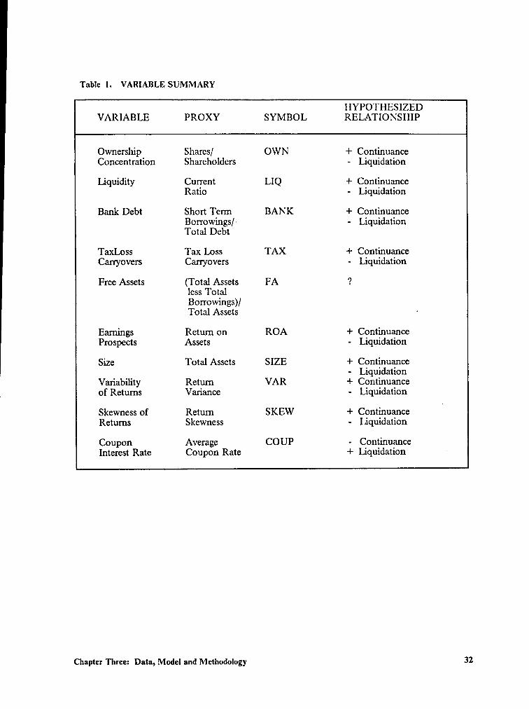
Table l. VARIABLE SUMMARY
IIYPOTHESIZEDVARIABLE PROXY SYMBOL RELATIONSIEIIP
Ownership Shares/ OWN + ContinuanceConcentration Shareholders - Liquidation
Liquidity Current LIQ + ContinuanceRatio - Liquidation
Bank Debt Short Tenn BANK + ContinuanceBorrowingsl- - LiquidationTotal Debt
TaxLoss Tax Loss TAX + ContinuanceCaxryovers Carryovers - Liquidation
Free Assets (Total Assets FA ?less TotalBorrowings)/Total Assets ·
Earnings Retum on ROA + ContinuanceProspects Assets - Liquidation
Size Total Assets SIZE + Continuance- Liquidation
Variability Retum VAR + Continuance_ of Returns Variance - Liquidation
Skewness of Retum SKEW + ContinuanceL
Retums Skewness - Liquidation
Coupon Average COUP - ContinuanceInterest Rate Coupon Rate + Liquidation
Chapter Three: Data, Model and Methodology 32

capital stock holdings and tax loss benefits of the firms are obtained from the Moody'si
Industrial Manual and the corporate 10-K reports of the firms. Data on the variance
and skewness of returns are obtained from the CRSP daily return liles.
While the size of the sample presents some statistical problems, it compares favor-
ably with the sample sizes of other studies in the area of bankruptcy (see Table 2). The
present sample is greater in size than all studies with the exception of White (1983) and
Clark and Weinstein (1983). White’s sample consisted of firms in the Southern District
of New York during her three year study period. Clark and Weinstein’s study used
market data for anperiod between 1938 and 1979.
Missing Data
Due to the nature of the firms under study and their state of financial distress, it
is not unexpected that observations for some of the variables are missing. The
Compustat and CRSP tapes have missing information for a number of the variables.
After searching other sources, missing data still remained. One method for dealing with
missing information for variables is to drop the observations for which there are missing
data. However, dropping the observations with partial data causes a loss of efliciency
and weakens the statistical statements that can be made about the estimated parameters
of the model. Further, the size of this sample requires that an alternative method for
dealing with the problem be found. An accepted method is the imputation of missing
Chapter Three: Data, Model and Mcthodology 33
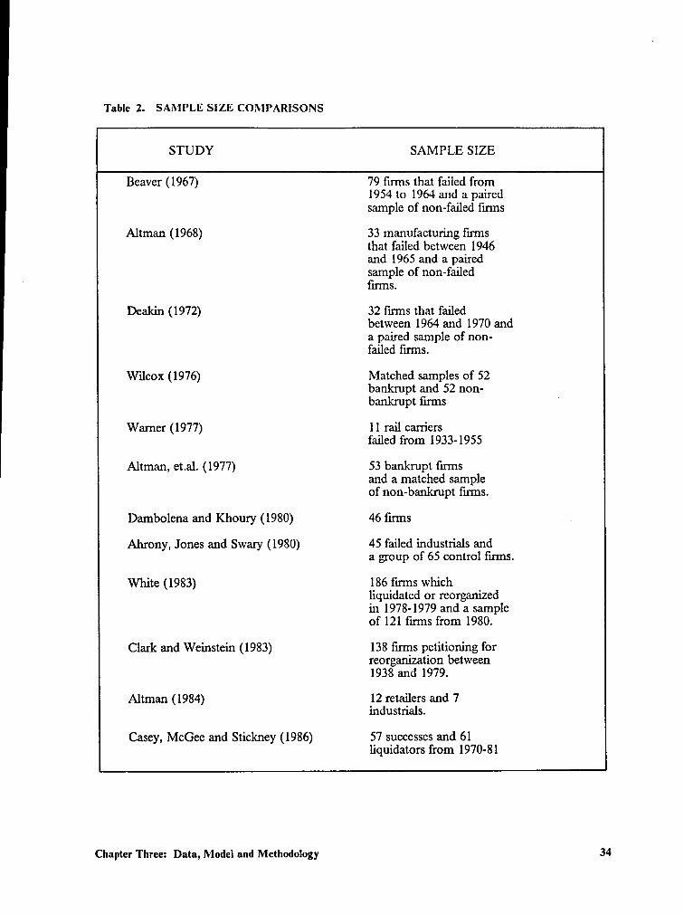
Table 2. SAl\·’lI’LE SIZE COMPARISONS
STUDY SAMPLE SIZE
Beaver (1967) 79 firms that failed from1954 to 1964 and a pairedsample of non-failed firms
Altman (1968) 33 manufacturing frrmsthat failed between 1946and 1965 and a pairedsample of non-failedfrrms.
Deakin (1972) 32 lirms that failedbetween 1964 and 1970 anda paired sample of non-failed iirms.
Wilcox (1976) Matched samples of 52banlcrupt and 52 non-bankmpt firms
Warner (1977) ll rail carnersfailed from 1933-1955
Altman, et.al. (1977) 53 bankrupt frrmsand a matched sampleof non-bankrupt frrrns.
Darnbolena and Khoury (1980) 46 frrms .
Ahrony, Jones and Swary (1980) 45 failed industrials anda group of 65 control firms.
White (1983) 186 firms whichliquidated or reorganizedin 1978-1979 and a sampleof 121 frrms from 1980.
Clark and Weinstein (1983) 138 frrms petitioning forreorganization between1938 and 1979.
Altman (1984) 12 retailers and 7industrials.
Casey, McGee and Stickney (1986) 57 successes and 61liquidators from 1970-81
Chapter Three: Data, Model and Methodology 34
data by the sample means? The missing data in this study are imputed by the sampleI
means by grouped outcome. The models were also run using data imputed by the
overall means for each variable with no significant difference in the results. The inter-
ested reader may refer to appendix B for the results of these runs. The univariate sta-
tistics for the variables by various groupings are given in Table 3.
Outcome Estimation Model
The decision of whether to use discriminant analysis or a conditional probability
model depends largely on the intended use of the results. lf dichotomous classification
is the only requirement, then discriminant analysis may be adequate, even though the
violation of statistical assumptions such as multivariate normality of the independent
variables may make evaluation sample specific. Discriminant analysis may also be used
to generate a probability, but most procedures to do so involve subjective assessment
of the probability associated with a particular discriminant score such as is done by
Altman in his Z-score analysis.
Conditional probability models such as logit and probit use the coefficients of the
independent variables to predict the probability of occurrence of a dichotomous de-
pendent variable. A cumulative probability distribution assumption is needed in order
to constrain the predicted values to comply with the acceptable (0,1) limiting values of
probability distributions. The coefficient of each variable can be interpreted as the effect
2 Robert S.Pindyck and Daniel L. Rubinfeld, Economctric Models & Economic Forcasts, (New York:McGraw-Hill, l98l),p.245-249.
Chapter Three: Data, Model and Mcthodology 35
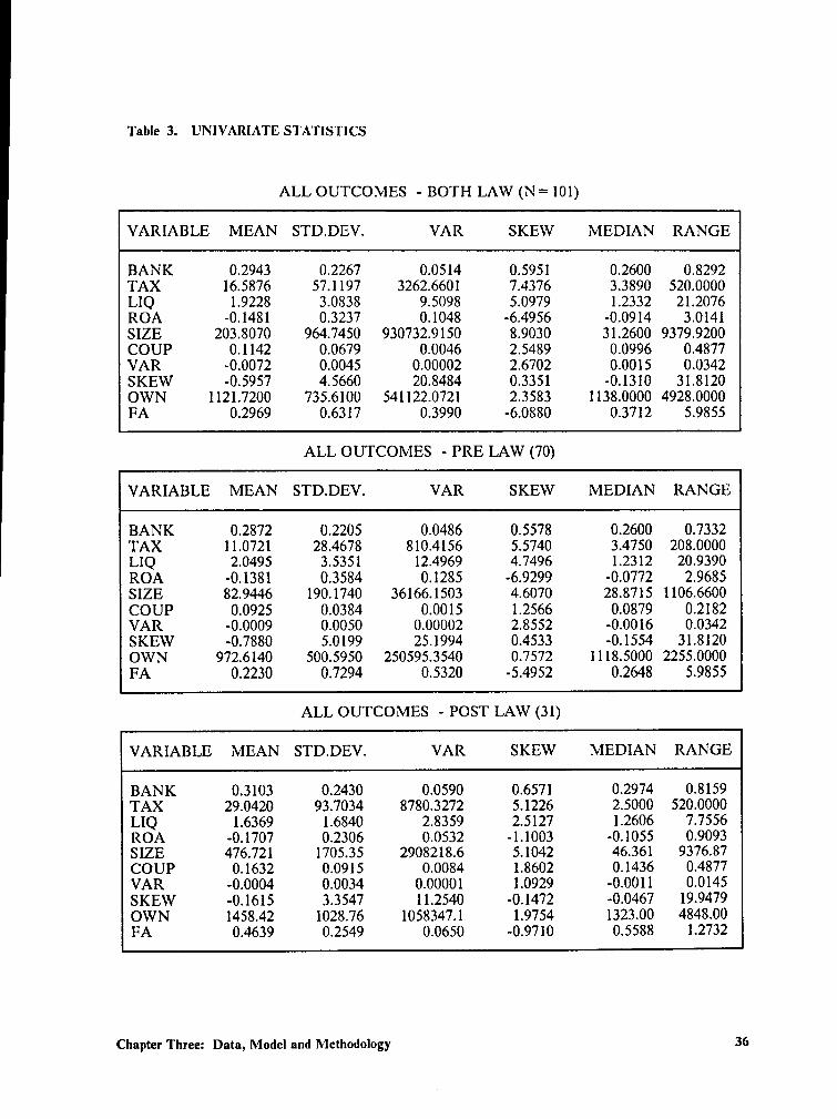
Table 3. UNIVARIATE STATISTICS
ALL OUTCOMES - BOTH LAW (N = 101)
VARIABLE MEAN STD.DEV. VAR SKEW MEDIAN RANGE
BANK 0.2943 0.2267 0.0514 0.5951 0.2600 0.8292TAX 16.5876 57.1 197 3262.6601 7.4376 3.3890 520.0000LIQ 1.9228 3.0838 9.5098 5.0979 1.2332 21.2076ROA -0.1481 0.3237 0.1048 -6.4956 -0.0914 3.0141SIZE 203.8070 964.7450 930732.9150 8.9030 31.2600 9379.9200COUP 0.1142 0.0679 0.0046 2.5489 0.0996 0.4877VAR -0.0072 0.0045 0.00002 2.6702 0.0015 0.0342SKEW -0.5957 4.5660 20.8484 0.3351 -0.1310 31.8120OWN 1121.7200 735.6100 $41122.0721 2.3583 1138.0000 4928.0000FA 0.2969 0.6317 0.3990 -6.0880 0.3712 5.9855
ALL OUTCOMES - PRE LAW (70)
VARIABLE MEAN STD.DEV. VAR SKEW MEDIAN RANGE
BANK 0.2872 0.2205 0.0486 0.5578 0.2600 0.7332TAX 11.0721 28.4678 810.4156 5.5740 3.4750 208.0000LIQ 2.0495 3.5351 12.4969 4.7496 1.2312 20.9390ROA -0.1381 0.3584 0.1285 -6.9299 -0.0772 2.9685SIZE 82.9446 190.1740 36166.1503 4.6070 28.8715 1106.6600COUP 0.0925 0.0384 0.0015 1.2566 0.0879 0.2182VAR -0.0009 0.0050 0.00002 2.8552 -0.0016 0.0342SKEW -0.7880 5.0199 25.1994 0.4533 -0.1554 31.8120OWN 972.6140 500.5950 250595.354O 0.7572 1118.5000 2255.0000FA 0.2230 0.7294 0.5320 -5.4952 0.2648 5.9855
ALL OUTCOMES - POST LAW (31)
VARIABLE MEAN STD.DEV. VAR SKEW MEDIAN RANGE
BANK 0.3103 0.2430 0.0590 0.6571 0.2974 0.8159TAX 29.0420 93.7034 8780.3272 5.1226 2.5000 520.0000LIQ 1.6369 1.6840 2.8359 2.5127 1.2606 7.7556ROA -0.1707 0.2306 0.0532 -1.1003 -0.1055 0.9093SIZE 476.721 1705.35 2908218.6 5.1042 46.361 9376.87COUP 0.1632 0.0915 0.0084 1.8602 0.1436 0.4877VAR -0.0004 0.0034 0.00001 1.0929 -0.0011 0.0145SKEW -0.1615 3.3547 11.2540 -0.1472 -0.0467 19.9479OWN 1458.42 1028.76 1058347.1 1.9754 1323.00 4848.00FA 0.4639 0.2549 0.0650 -0.9710 0.5588 1.2732
Chapter Three: Data, Modcl and Methodology 36
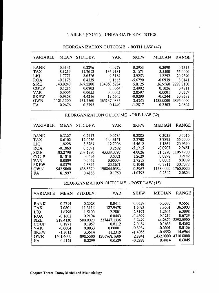
TABLE 3 (CONT) - UNIVARIATE STATISTICS
REORGANIZATION OUTCOME - BOTII LAW (47)
VARIABLE MEAN STD.DEV. VAR SKEW MEDIAN RANGE
BANK 0.3131 0.2296 0.0527 0.2953 0.3090 0.7315TAX 8.1219 11.7012 136.9181 2.1371 3.5500 55.0000LIQ 1.7771 3.0526 9.3184 5.9253 1.2292 20.9390ROA -0.1178 0.4339 0.1883 -5.6790 -0.0939 3.0141SIZE 140.0240 367.2200 I34850.5284 5.0125 36.9560 2297.8100COUP 0.1285 0.0803 0.0064 ‘· 2.4902 0.1026 0.4811VAR 0.0005 0.0055 0.00003 2.8597 0.0001 0.0309SKEW -0.9858 4.4216 19.5505 -0.0290 -0.6244 30.7378OWN 1121.1500 751.7560 $65137.0835 3.4345 1138.0000 4895.0000FA 0.2676 0.3795 0.1440 -1.2817 0.2503 2.0804
REORGANIZATION OUTCOME - PRE LAW (32)
VARIABLE MEAN STD.DEV. VAR SKEW MEDIAN RANGE
BANK 0.3327 0.2417 0.0584 0.2885 0.3035 0.7315TAX 8.6102 12.0256 144.6151 2.3708 3.7895 55.0000LIQ 1.8228 3.5764 12.7906 5.4612 1.1861 20.9390ROA -0.1860 0.5091 0.2592 -5.2715 -0.0907 2.9451SIZE 103.2790 208.1780 43338.0797 4.0026 31.3270 1106.1200COUP 0.1010 0.0456 0.0021 1.2629 0.0898 0.2182VAR 0.0009 0.0062 0.00004 2.7215 0.0003 0.0309SKEW -0.8379 4.8854 23.8671 0.1040 -0.7811 30.7378OWN 942.9060 436.8570 I90844.0384 0.3967 1138.0000 1760.0000FA 0.1997 0.4183 0.1750 -1.0793 0.2342 2.0804
REORGANIZATION OUTCOME - POST LAW (15)
VARIABLE MEAN STD.DEV. VAR SKEW MEDIAN RANGE
BANK 0.2714 0.2028 0.0411 0.0559 0.3090 0.5551TAX 7.0801 11.3114 127.9478 1.7093 3.3501 36.5000LIQ 1.6798 1.5100 2.2801 2.8197 1.2606 6.3098ROA -0.1602 0.2104 0.0443 -0.4699 -0.1219 0.6729SIZE 218.4130 580.9020 337447.1336 3.7479 44.2670 2292.0000COUP 0.1871 0.1057 0.0112 2.0084 0.1633 0.4302VAR -0.0004 0.0033 0.00001 0.8934 -0.0001 0.0136SKEW -1.3013 3.3514 11.2319 -1.4055 -0.4552 14.6964OWN 1501.4000 1098.5300 1206768.1609 2.8941 1432.0000 4710.0000FA 0.4124 0.2299 0.0529 -0.2897 0.4414 0.6045
Chapter Three: Data, Model and Methodology 37
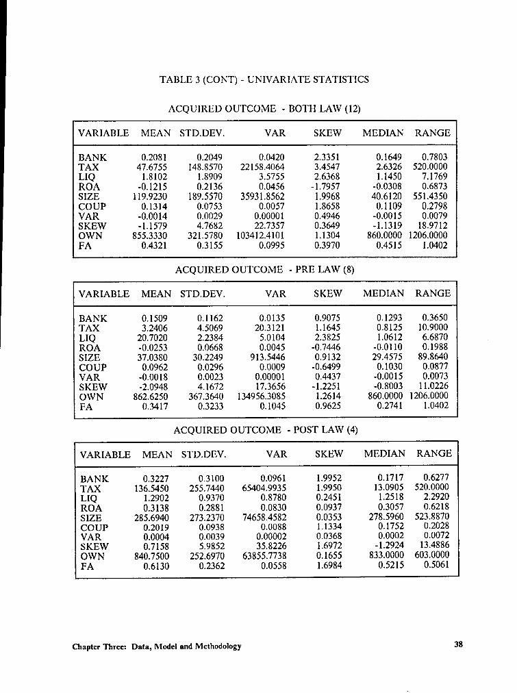
TABLE 3 (CONT) - UNIVARIATE STATISTICS
ACQUIRED OUTCOME - BOT1·I LAW (12)
VARIABLE MEAN STD.DEV. VAR SKEW MEDIAN RANGE
BANK 0.2081 0.2049 0.0420 2.3351 0.1649 0.7803TAX 47.6755 148.8570 22158.4064 3.4547 2.6326 520.0000LIQ 1.8102 1.8909 3.5755 2.6368 1.1450 7.1769ROA -0.1215 0.2136 0.0456 -1.7957 -0.0308 0.6873SIZE 119.9230 189.5570 35931.8562 1.9968 40.6120 551.4350COUP 0.1314 0.0753 0.0057 1.8658 0.1109 0.2798VAR -0.0014 0.0029 0.00001 0.4946 -0.0015 0.0079SKEW -1.1579 4.7682 22.7357 0.3649 -1.1319 18.9712OWN 855.3330 321.5780 103412.410I 1.1304 860.0000 1206.0000FA 0.4321 0.3155 0.0995 0.3970 0.4515 1.0402
ACQUIRED OUTCOME - PRE LAW (8)
VARIABLE MEAN STD.DEV. VAR SKEW MEDIAN RANGE
BANK 0.1509 0.1162 0.0135 0.9075 0.1293 0.3650TAX 3.2406 4.5069 20.3121 1.1645 0.8125 10.9000LIQ 20.7020 2.2384 5.0104 2.3825 1.0612 6.6870ROA -0.0253 0.0668 0.0045 -0.7446 -0.0110 0.1988SIZE 37.0380 30.2249 913.5446 0.9132 29.4575 89.8640COUP 0.0962 0.0296 0.0009 -0.6499 0.1030 0.0877VAR -0.0018 0.0023 0.00001 0.4437 -0.0015 0.0073SKEW -2.0948 4.1672 17.3656 -1.2251 -0.8003 11.0226OWN 862.6250 367.3640 134956.3085 1.2614 860.0000 1206.0000FA 0.3417 0.3233 0.1045 0.9625 0.2741 1.0402
ACQUIRED OUTCOME - POST LAW (4)
VARIABLE MEAN STD.DEV. VAR SKEW MEDIAN RANGE
BANK 0.3227 0.3100 0.0961 1.9952 0.1717 0.6277TAX 136.5450 255.7440 65404.9935 1.9950 13.0905 520.0000LIQ 1.2902 0.9370 0.8780 0.2451 1.2518 2.2920ROA 0.3138 0.2881 0.0830 0.0937 0.3057 0.6218SIZE 285.6940 273.2370 74658.4582 0.0353 278.5960 523.8870COUP 0.2019 0.0938 0.0088 1.1334 0.1752 0.2028VAR 0.0004 0.0039 0.00002 0.0368 0.0002 0.0072SKEW 0.7158 5.9852 35.8226 1.6972 -1.2924 13.4886OWN 840.7500 252.6970 63855.7738 0.1655 833.0000 603.0000FA 0.6130 0.2362 0.0558 1.6984 0.5215 0.5061
Chapter Three: Data, Model and Methodology 38
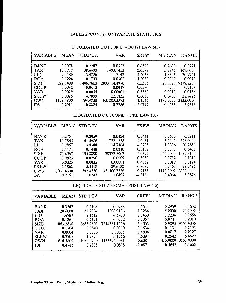
TABLE 3 (CONT) - UNIVARIATE STATISTICS
LIQUIDATED OUTCOME - BOTH LAW (42)
VARIABLE MEAN STD.DEV. VAR SKEW MEDIAN RANGE
BANK 0.2978 0.2287 0.0523 0.6523 0.2600 0.8271TAX 17.1789 38.6490 1493.7452 3.6579 3.2945 208.0000LIQ 2.1180 3.4226 11.7142 4.4633 1.3306 20.7721ROA 0.1226 0.1739 0.0302 -1.8082 0.0867 0.9010SIZE 299.1490 1446.7600 2093114.4976 6.3365 28.8320 9379.7200COUP 0.0932 0.0413 0.0017 0.9570 0.0900 0.2193VAR 0.0019 0.0034 0.00001 * 0.3362 0.0019 0.0186SKEW 0.0015 4.7099 22.1832 0.6656 0.0467 28.7485OWN 1198.4800 794.4830 63l203.2373 1.1546 1175.0000 3233.0000FA 0.2911 0.8824 0.7786 -5.4717 0.4538 5.9576
LIQUIDATED OUTCOME - PRE LAW (30)
VARIABLE MEAN STD.DEV. VAR SKEW MEDIAN RANGE
BANK 0.2751 0.2059 0.0424 0.5441 0.2600U
0.7311TAX 15.7865 41.4986 1722.1338 4.0481 3.2945 208.0000LIQ 2.2857 3.8388 14.7364 4.3285 1.3306 20.2659ROA 0.1171 0.1448 0.0210 0.8102 0.0893 0.5433SIZE 73.4967 195.8890 38372.5003 5.0392 25.9900 1079.3100COUP 0.0823 0.0296 0.0009 0.5959 0.0782 0.1210VAR 0.0025 0.0032 0.00001 0.4759 0.0019 0.0124SKEW 0.3863 5.4418 29.6132 0.8082 0.0467 28.7485OWN 1033.6300 592.8750 351500.7656 0.7188 1175.0000 2255.0000FA 0.2161 1.0243 1.0492 -4.8166 0.4064 5.9576
LIQUIDATED OUTCOME — POST LAW (12)
VARIABLE MEAN STD.DEV. VAR SKEW MEDIAN RANGE
BANK 0.3547 0.2798 0.0783 0.5543 0.2959 0.7652TAX 20.6600 31.7634 1008.9136 1.7286 5.0000 99.0000LIQ 1.6987 2.1312 4.5420 2.3460 1.2204 7.7556ROA 0.1361 0.2391 0.0572 -2.3067 0.0741 0.9010SIZE 863.2810 2685.9600 7214381.1216 3.4503 40.9895 9363.9000COUP 0.1204 0.0540 0.0029 0.1534 0.1131 0.2193VAR 0.0004 0.0035 0.00001 1.8898 0.0017 0.0127SKEW 0.9708 1.7823 3.1766 1.5097 0.2942 5.6822OWN 1610.5800 4 1080.0900 1166594.4081 0.6081 1415.0000 3153.0000FA 0.4785 0.2878 0.0828 -2.0871 0.5642 1.1663
Chapter Three: Data, Model and Mcthodology 39
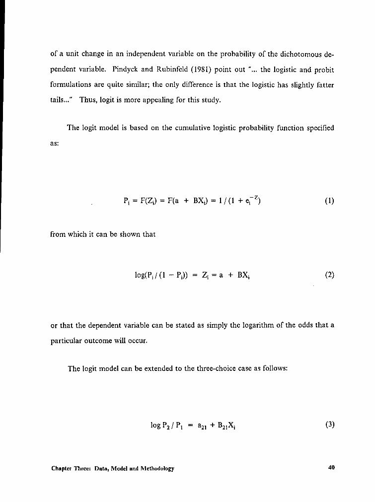
of a unit change in an independent variable on the probability of the dichotomous de-
pendent variable. Pindyck and Rubinfcld (1981) point out the logistic and probit
formulations are quite similar; the only difference is that the logistic has slightly fatter
tails..." Thus, logit is more appealing for this study.
The logit model is based on the cumulative logistic probability function specified
as:
. Pi = F(Zi) = Flä + BXi) = 1/(1 + @[2) (1)
from which it can be shown that
" = Zi = H+or
that the dependent variable can be stated as simply the logarithm of the odds that a
particular outcome will occur.
The logit model can be extended to the three-choice case as followsz
log P2/P1 = am + B21Xi (3)
Chapter Three: Data, Model and Methodology 40
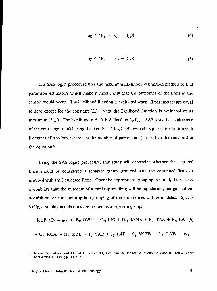
JOE P3/P1 = aai + Bsixi (4)
log P3 / P2 = a32 + B32Xi (5)
The SAS logist procedure uses the maximum likelihood estimation method to find
parameter estimators which make it most likely that the outcomes of the firms in the
sample would occur. The likelihood function is evaluated when all parameters are equal
to zero except for the constant (Lo). Next the likelihood function is evaluated at its
maximum (LM,). The likelihood ratio K is defined as L,/L,„,,,. SAS tests the significance
of the entire logit model using the fact that -2 log ?„ follows a chi-square distribution with
k degrees of freedom, where k is the number of parameters (other than the constant) in
the equation.3
Using the SAS logist procedure, this study will determine whether the acquired
firms should be considered a separate group, grouped with the continued firms or
grouped with the liquidated firms. Once the appropriate grouping is found, the relative
probability that the outcome of a bankruptcy filing will be liquidation, reorganization,
acquisition, or some appropriate grouping of these outcomes will be modeled. Specif-
ically, assuming acquisitions are treated as a separate group:
log P2/P, = a2, + B2, OWN + C2, LIQ + D2, BANK + E2, TAX + F2, FA (6)
+ G2, ROA + H2, SIZE + I2, VAR + J2, INT + K2, SKEW + L2, LAW + e2,
3 Robert S.Pindyck and Daniel L. Rubinfeld, Econometric Models & Economic Forcasts, (New York:McGraw-Hill, 198l),p.3l1-312.
Chapter Three: Data, Model and Methodology 41
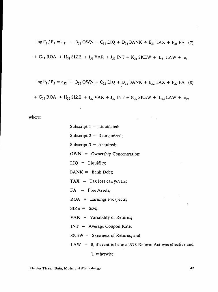
log P3/P, = a3, + B3, OWN + C3, LIQ + D3, BANK + E3, TAX + F3, FA (7)
+ G3, ROA + I··I3, SIZE + I3, VAR + J3, INT + K3, SKEW + L3, LAW + e3,
log P3/P2 = a32”+
B32 OWN + C32 LIQ + D32 BANK + E32 TAX + F32 FA (8)
+ G32 ROA + H32 SIZE + 132 VAR + .1321NT + K32 SKEW + L32 LAW + e32
where: „ ' [
Subscript 1 = Liquidated;
Subscript 2 = Reorganized;
Subscript 3 = Acquired;
OWN = Owncrship Concentration;I
LIQ = Liquidity; -
BANK = Bank Debt;
TAX = Tax loss carryovers;
FA = Free Assets;
ROA = EarningsProispects;SIZE
= Size;
VAR = Variability of Returns;
INT = Average Coupon Rate;
SKEW = Skewness of Returns; and
LAW = 0; if event is before 1978 Reform Act was effective and
I, uotherwise.
Chapter Three: Data, Model and Methodology 42
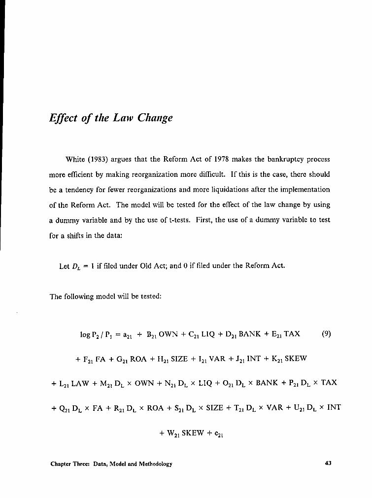
Ej§’ect of the Law Change
White (1983) argues that the Reform Act of 1978 makes the bankruptcy process
more eflicient by making reorganization more diflicult. If this is the case, there should
be a tendency for fewer reorganizations and more liquidations after the implementation
of the Reform Act. The model will be tested for the effect of the law change by using
a dummy variable and by the use of t-tests. First, the use of a dummy variable to test
for a shifts in the data:
Let DL = 1 if filed under Old Act; and 0 if filed under the Reform Act.
The following model will be tested:
log P2/ P, = a2, + B2, OWN + C2, LIQ + D2, BANK + E2, TAX (9)
+ F2, FA + G2, ROA + I”I2l SIZE + I2, VAR + J2, INT + K2, SKEW
+ L2, LAW + M2, DL X OWN + N2, DL X LIQ + O2, DL X BANK + P2, DL X TAX
+ Q2, DL X FA + R2, DL X ROA + S2, DL X SIZE + T2, DL X VAR + U2, DL X INT
+ W2, SKEW + 821
Chapter Three: Data, Model and Methodology 43
where:
Subscript l = Liquidated
Subscript 2 = Continucd
Should any of' the interactive coeflicients be significant, there is an indication that the
law change has an effect. The model is run for the continued versus liquidated groups
only, due to the limited size of the acquired group. This grouping is intuitively appealing
because of the similarity of the consequences to the claimants.
Next, an additional set of tests are run to see if there are differences in the variables
of the model across the law change. T—tests are run on the data to determine if there
are significant differences in the means of the variables when grouped according to the
set of laws the firms filed under. These t-tests arc conducted for all possible groupings
of the data. The SAS t-test procedure first tests for equal variances and then presents
the t-tests for equal means for both the equal variance and the unequal variance cases.
This chapter has presented the motivation of the variables, the development of the
model, the sample selection and the statistical methodology. Next, the results of the
study are presented.
Chapter Three: Data, Model and Methodology 44
Chapter Four: Results
Introduction
The results of the statistical analyses are presented in this chapter. First, the results
of the analyses to determine the proper grouping of the acquired firms are presented.
Next, the results of the analysis comparing liquidated firms to reorganized firms are
given along with the effects that the significant variables have on the disposition of the
bankrupt firm. Then, the acquired firms are grouped with the reorganized firms and
results for the liquidated versus "continued” firms are given. Finally, the results of the
tests for the effect of the law change are presented.
Chapter Four: Results 45
Catcgorization ofAcquired Firms
Acquired Versus Liquidated
A central question in this study concerns thelcategorization of acquired firms. That
is, whether they can be classified as liquidated, reorganized, or whether they are a sta-
tistically different sub—group. To answer this question, pairwise logit models are esti-
mated for both acquired versus liquidated groups and acquired versus reorganized
groups. The results of the logit analysis of the 12 acquired and 42 liquidated firms are
presented in Table 4. According to the chi- square statistic of 15.55 (11 df) the model
is signilicant at only the ot = 0.1585 level. While the model as a whole does not statis-
tically distinguish between the acquired and liquidated lirms at a level that is statistically
acceptable, the average coupon rate variable (COUP) is significant at the ot = 0.0658
level and is positively signed. This indicates that the higher the coupon rate, the greater
the likelihood of acquisition. Further, the ownership concentration variable (OWN) is
significant at the ot = 0.0271 level with a negative BETA, indicating that the lower the
ownership concentration, the greater the likelihood of acquisition.
The coupon rate effect is in direct opposition to Bulow and Shoven's argument that
the greater the need for funds from banklenders, the less likely they will provide these
funds, making liquidation more likely. One explanation for this anomaly is that the av-
erage coupon rate is proxying for interest rates. To test this possibility, the average
coupon rate is divided by the market fatc of interest at the time of filing. Both the
Chapter Four: Results 46
Corporate Baa rate and the prime rate are used.‘ The results presented in Table 5 reveal
that regardless which rate is used to adjust the coupon rate, the interest rate variable
‘
(INT) drops in significance. For the Baa adjustment, the interest rate variable (INT), is
significant at only the oz = 0.1176 level and the variance of returns variable (VAR) enters
the model at a signiflcance level of ot = 0.0751. When adjusted with the prime rate, the
INT variable is significant only at the ci = 0.0968 level but the variance of returns vari-
able (VAR) is only significant at a level of cx = 0.1054. In both cases, the coefficient of
the variance of returns has the hypothesized sign.
The ownership concentration effect is also opposite to that expected. However, to
the extent that low ownership concentration implies less management control, the re-
lationship is as hypothesized from an agency perspective.
The t-tests for differences in the means of the variables grouped by liquidated out-
come versus acquired outcome presented in Table 6 support the logit findings. The
coupon interest variable (COUP) is found to have statistically different means at the
tz = 0.0245 level with coupon interest rate being higher for the acquired firms. The
ownership concentration variable (OWN) has means that are significantly different at
the oz = 0.1519 level with higher concentration for the liquidated firms.
The above results indicate that there are significant differences in the coupon in-
terest rate, ownership concentration and variance of returns variables for acquired firms
versus liquidated tirms. Thus, White should not have combined the two groups in her
1983 study.
‘The interest rates used are those in effect at the time of filing and were found in "The Economic Reportof the President', United States Government Printing Oflice, Jan. 1987
Chapter Four: Results 47
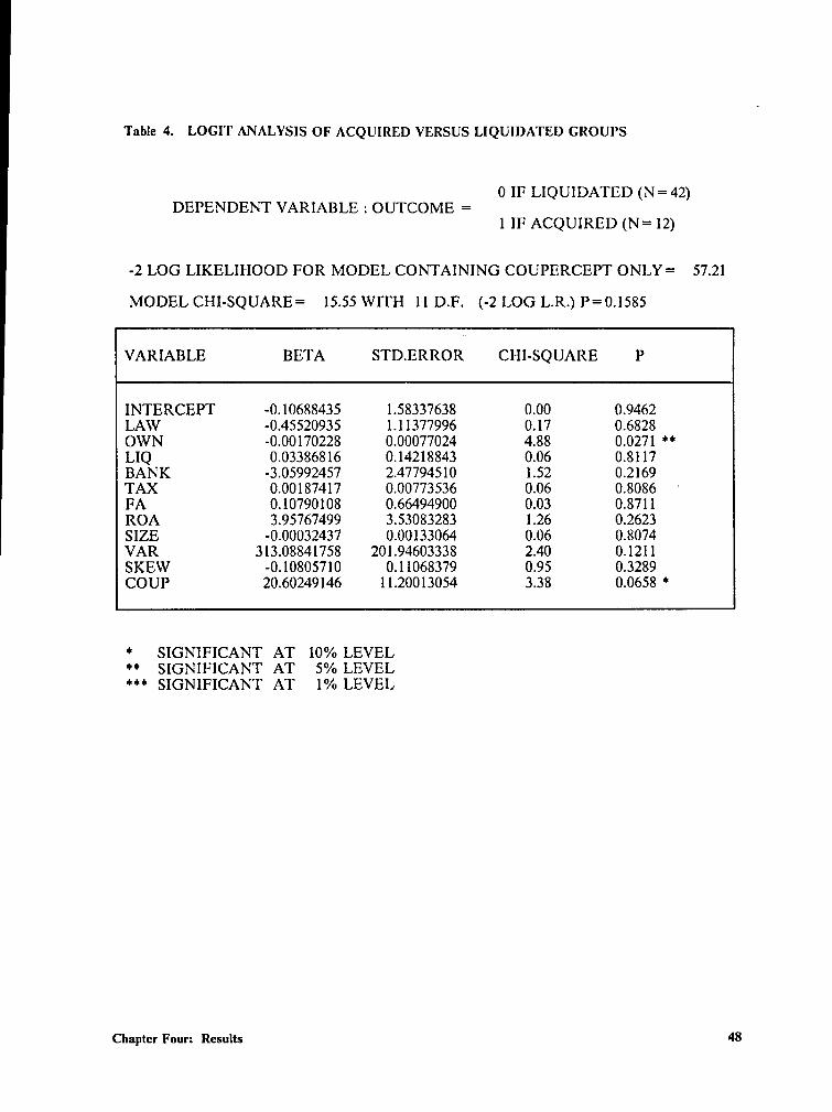
Table 4. LOGl'l‘ ANALYSIS OF ACQUIRED VERSUS LIQUIDATED GROUPS
0 IF LIQUIDATED (N = 42)DEPENDENT VARIABLE 2 OUTCOME =
1 IF ACQUIRED (N= 12)
-2 LOG LIKELIHOOD FOR MODEL CONTAINING COUPERCEPT ONLY= 57.21
MODEL CHI-SQUARE= 15.55 WITH 11 D.F. (-2 LOG L.R.) P=0.1585
VARIABLE BETA STD.ERROR CHI-SQUARE P
INTERCEPT -0.10688435 1.58337638 0.00 0.9462LAW -0.45520935 1.11377996 0.17 0.6828OWN -0.00170228 0.00077024 4.88 0.0271 **LIQ 0.03386816 0.14218843 0.06 0.8117BANK -3.05992457 2.47794510 1.52 0.2169TAX 0.00187417 0.00773536 0.06 0.8086 ‘FA 0.10790108 0.66494900 0.03 0.8711ROA 3.95767499 3.53083283 1.26 0.2623SIZE -0.00032437 0.00133064 0.06 0.8074VAR 3 13.0884l758 201.94603338 2.40 0.1211SKEW -0.10805710 0.11068379 0.95 0.3289COUP 20.60249146 11.20013054 3.38 0.0658 *
* SIGNIFICANT AT 10% LEVEL** SIGNIFICANT AT 5% LEVEL*** SIGNIFICANT AT 1% LEVEL
Chapter Four: Results 48
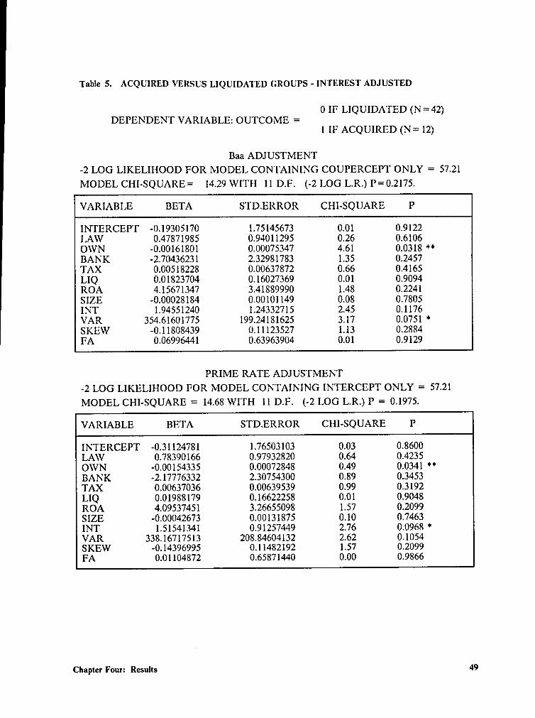
Table 5. ACQUIRED VERSUS LIQUIDATED GROUPS - INTEREST ADJUSTED
0 IF LIQUIDATED (N = 42)DEPENDENT VARIABLE: OUTCOME =
1 IF ACQUIRED (N= 12)
Baa ADJUSTMENT-2 LOG LIKELIHOOD FOR MODEL CONTAINING COUPERCEPT ONLY = 57.21MODEL CIII-SQUARE= 14.29 WITH 11 D.F. (-2 LOG L.R.) P= 0.2175.
VARIABLE BETA STD.ERROR CHI-SQUARE P
INTERCEPT -0.19305170 1.75145673 0.01 0.9122LAW 0.47871985 0.94011295 0.26 0.6106OWN -0.0016180I 0.00075347 4.61 0.0318 **BANK -2.7043623l 2.32981783 1.35 0.2457TAX 0.00518228 0.00637872 0.66 0.4165LIQ 0.01823704 0.16027369 0.01 0.9094ROA 4.15671347 3.41889990 1.48 0.2241SIZE —0.00028184 0.00101149 0.08 0.7805INT 1.94551240 1.24332715 2.45 0.1176VAR 354.61601775 199.24181625 3.17 0.0751 *SKEW -0.11808439 0.11123527 1.13 0.2884FA 0.06996441 0.63963904 0.01 0.9129
PRIME RATE ADJUSTMENT-2 LOG LIKELIHOOD FOR MODEL CONTAINING INTERCEPT ONLY = 57.21
MODEL CHI—SQUARE = 14.68 WITH 11 D.F. (-2 LOG L.R.) P = 0.1975.
VARIABLE BETA STD.ERROR CHI-SQUARE P
INTERCEPT -0.31124781 1.76503103 0.03 0.8600LAW 0.78390166 0.97932820 0.64 0.4235OWN -0.0015433S 0.00072848 0.49 0.0341 **BANK -2.17776332 2.30754300 0.89 0.3453TAX 0.00637036 0.00639539 0.99 0.3192LIQ 0.01988179 0.16622258 0.01 0.9048ROA 4.09537451 3.26655098 1.57 0.2099SIZE -0.00042673 0.00131875 0.10 0.7463INT 1.51541341 0.91257449 2.76 0.0968 *VAR 338.16717513 208.84604132 2.62 0.1054SKEW -0.14396995 0.11482192 1.57 0.2099FA 0.01104872 0.65871440 0.00 0.9866
Chapter Four: Results 49
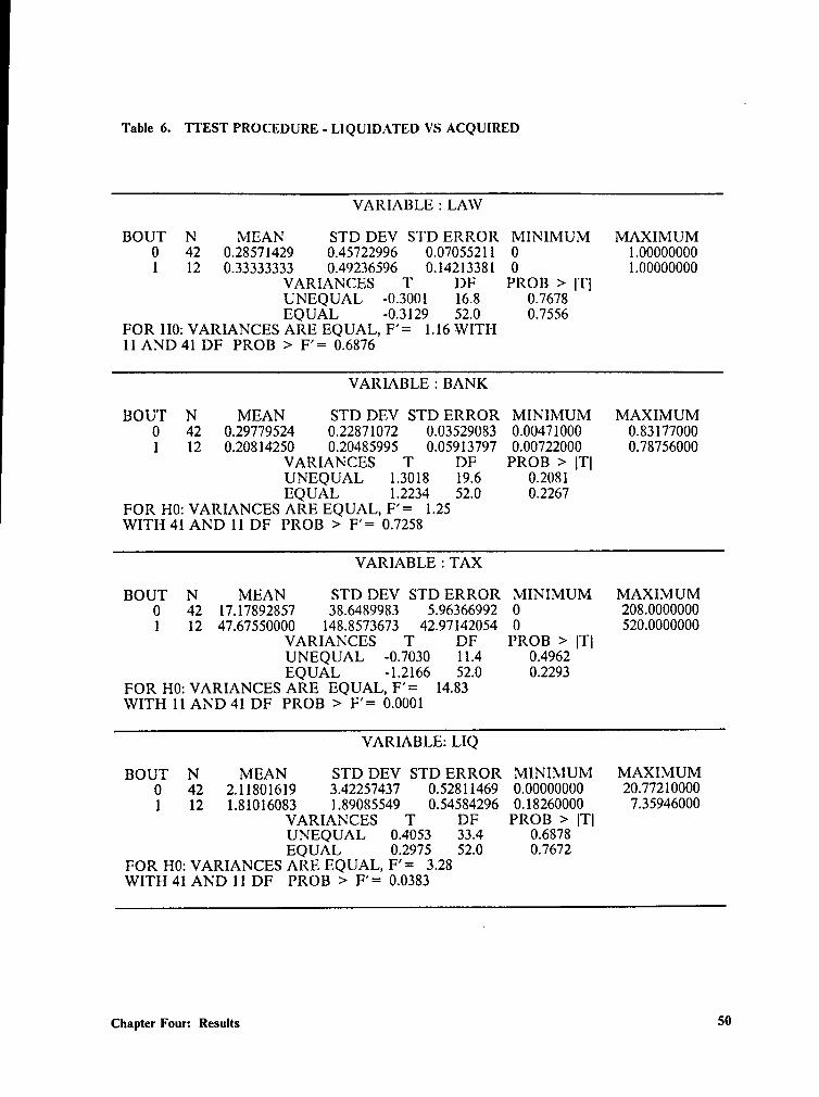
Table 6. TTEST PROCEDURE - LIQUIDATED VS ACQUIRED
VARIABLE : LAW
BOUT N MEAN STD DEV STD ERROR MINIMUM MAXIMUM0 42 0.28571429 0.45722996 0.07055211 0 1.000000001 12 0.33333333 0.49236596 0.14213381 0 1.00000000
VARIANCES T DF PROB > |TlUNEQUAL -0.3001 16.8 0.7678EQUAL -0.3129 52.0 0.7556
FOR H0: VARIANCES ARE EQUAL, F’= 1.16 WITH11 AND 41 DF PROB >
F’=0.6876
VARIABLE : BANK
BOUT N MEAN STD DEV STD ERROR MINIMUM MAXIMUM0 42 0.29779524 0.22871072 0.03529083 0.00471000 0.831770001 12 0.20814250 0.20485995 0.05913797 0.00722000 0.78756000
VARIANCES T DF PROB > lT|UNEQUAL 1.3018 19.6 0.2081EQUAL 1.2234 52.0 0.2267
FOR H0: VARIANCES ARE EQUAL, F’= 1.25WITH 41 AND 11 DF PROB >
F’=0.7258
VARIABLE : TAX
BOUT N MEAN STD DEV STD ERROR MINIMUM MAXIMUM0 42 17.17892857 38.6489983 5.96366992 0 20800000001 12 47.6755000O 148.8573673 42.97142054 0 $20.0000000
VARIANCES T DF PROB > |T|UNEQUAL -0.7030 11.4 0.4962EQUAL -1.2166 52.0 0.2293
FOR H0: VARIANCES ARE EQUAL, F’= 14.83WITH 11 AND 41 DF PROB > F’= 0.0001
‘ VARIABLE: LIQ
BOUT N MEAN STD DEV STD ERROR MINIMUM MAXIMUM0 42 2.11801619 3.42257437 0.52811469 0.00000000 20.7721000O1 12 1.81016083 1.89085549 0.54584296 0.18260000 7.35946000
VARIANCES T DF PROB > lT|UNEQUAL 0.4053 33.4 0.6878EQUAL 0.2975 52.0 0.7672
FOR H0: VARIANCES ARE EQUAL, F’= 3.28WITH 41 AND 11 DF PROB >
F’=0.0383
Chapter Four: Results 50
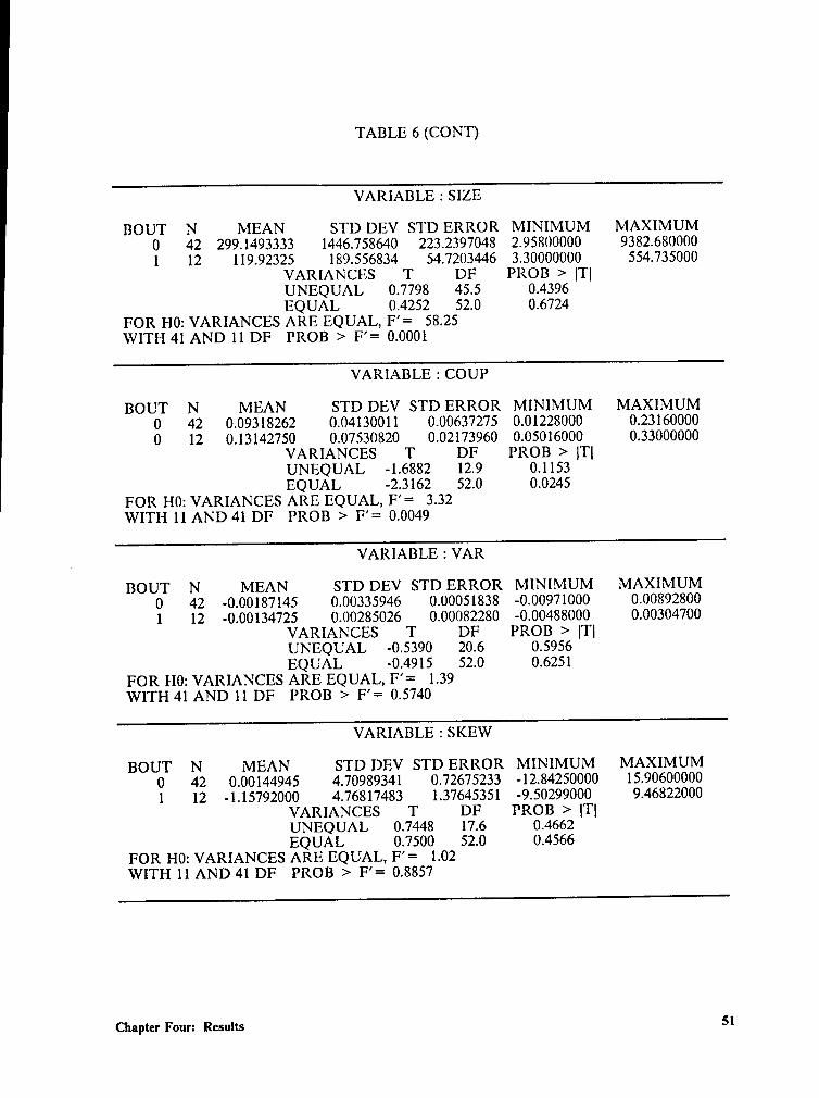
TABLE 6 (CONT)
VARIABLE : SIZE
BOUT N MEAN STD DEV STD ERROR MINIMUM MAXIMUM0 42 299.1493333 1446.758640 223.2397048 2.95800000 9382.6800001 12 119.92325 189.556834 54.7203446 3.30000000 554.735000
VARIANCES T DF PROB > |T|UNEQUAL 0.7798 45.5 0.4396EQUAL 0.4252 52.0 0.6724
FOR H0: VARIANCES ARE EQUAL, F’= 58.25VVITH 41 AND 11 DF PROB > F'= 0.0001
VARIABLE : COUP
BOUT N MEAN STD DEV STD ERROR MINIMUM MAXIMUM0 42 0.09318262 0.04130011 0.00637275 0.01228000 0.231600000 12 0.13142750 0.07530820 0.02173960 0.05016000 0.33000000
VARIANCES T DF PROB > |T|UNEQUAL -1.6882 12.9 0.1153EQUAL -2.3162 52.0 0.0245
FOR H0: VARIANCES ARE EQUAL,F’=
3.32WITH 11 AND 41 DF PROB >
F’=0.0049
VARIABLE : VAR
BOUT N MEAN STD DEV STD ERROR MINIMUM MAXIMUM0 42 -0.00187145 0.00335946 0.00051838 -0.00971000 0.008928001 12 -0.00134725 0.00285026 0.00082280 -0.00488000 0.00304700
VARIANCES T DF PROB > |T|UNEQUAL -0.5390 20.6 0.5956EQUAL -0.4915 52.0 0.6251
FOR H0: VARIANCES ARE EQUAL, F'= 1.39WITH 41 AND 11 DF PROB > F'= 0.5740
VARIABLE : SKEW
BOUT N MEAN STD DEV STD ERROR MINIMUM MAXIMUM0 42 0.00144945 4.70989341 0.72675233 -12.84250000 15.9060000O1 12 -1.15792000 4.76817483 1.37645351 -9.50299000 9.46822000
VARIANCES T DF PROB > |T|UNEQUAL 0.7448 17.6 0.4662EQUAL 0.7500 52.0 0.4566
FOR H0: VARIANCES ARE EQUAL,F’=
1.02WITH 11 AND 41 DF PROB > F’= 0.8857
Chapter Four: Results 51
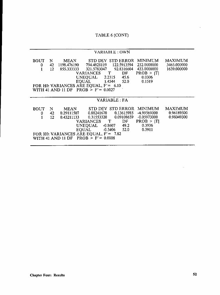
TABLE 6 (CONT)
VARIABLE : OWN
BOUT N MEAN STD DEV STD ERROR MINIMUM MAXIMUM0 42 1198.47619O 794.4828119 122.5913594 232.0000000 3465.0000001 12 855.333333 321.5783047 92.8316604 433.0000000 1639.000000
VARIANCES T DF PROB > |T|UNEQUAL 2.2315 45.6 0.0306EQUAL 1.4544 52.0 0.1519
FOR H0: VARIANCES ARE EQUAL,F’=
6.10WITH 41 AND 11 DF PROB > F’= 0.0027
“
VARIABLE : FA
BOUT N MEAN STD DEV STD ERROR MINIMUM MAXIMUM0 42 0.29111507 0.88241670 0.13615985 -4.99569000 0.961895001 12 0.43211133 0.31553320 0.09108659 -0.05973000 0.98049300
VARIANCES T DF PROB > [TlUNEQUAL -0.8607 49.2 0.3936EQUAL -0.5406 52.0 0.5911
FOR H0: VARIANCES ARE EQUAL, F’= 7.82WITH 41 AND 11 DF PROB > F’= 0.0008
Chapter Four: Results 52
Acquired Versus Reorganizerl
The results of the logit analysis for the 47 reorganized and 12 acquired firms are
presented in Table 7. The chi-square statistic of ll.05 (11 df) shows that the model is
significant at only the ot = 0.4391 level. Further, none of the variables in the model
significantly differentiate between reorganized and acquired firms} The t-tests in Table
8 find that no variable has means significantly different at the ot = .05 level when
grouped by acquired versus reorganized outcomes. The tax loss carryover variable
(TAX) has significantly different means between the acquired versus reorganized groups
only at the ot = 0.070 level.
Overall, the results indicate that there is no statistical difference between the reor-
ganized firms and the acquired firms. This is in direct opposition to White's grouping
and further supports the findings of the previous section that the acquired firms should
not be grouped with the liquidated firms. The results of the analyses of the acquired
versus liquidated firms and acquired versus reorganized firms show that, by not including
the acquired firms, Casey, McGee, and Stickney unnecessarily reduced the size of their
sample.
S The model was estimated using the coupon rate adjusted for the level of interest rates at the time of liling.Since the insignificance of the variables remains the same, the results are not reported here.
Chapter Four: Results 53
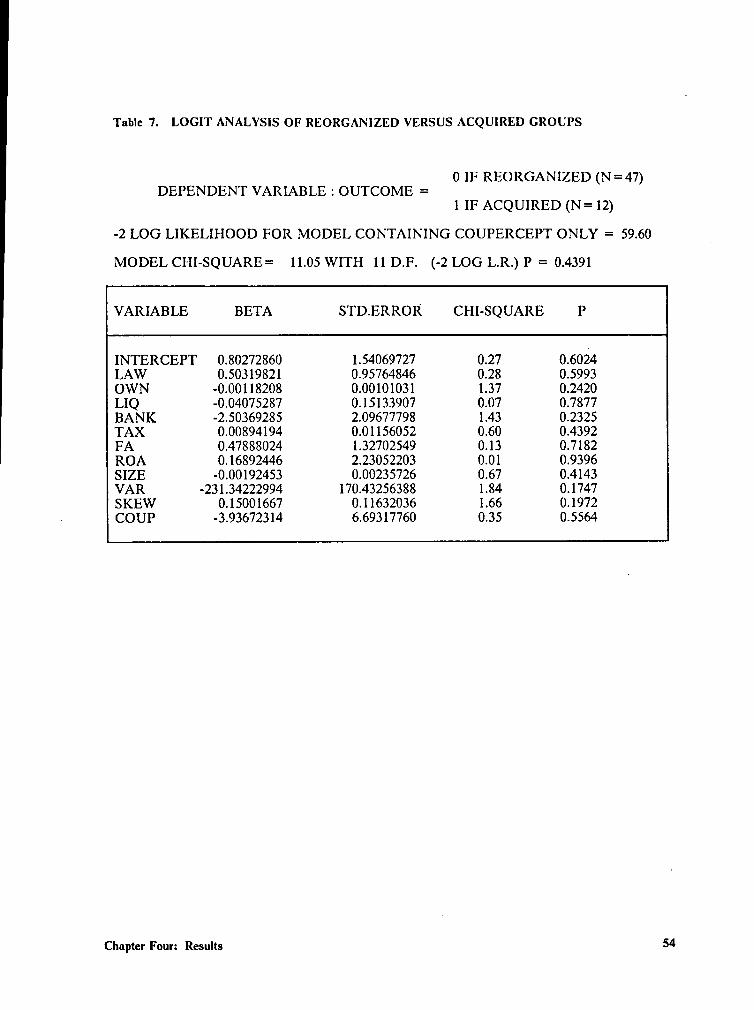
Table 7. LOGIT ANALYSIS OF REORGANIZED VERSUS ACQUIRED GROUPS
0 IF REORGANIZED (N=47)DEPENDENT VARIABLE : OUTCOME =
1 IF ACQUIRED (N= 12)
-2 LOG LIKELIHOOD FOR MODEL CONTAINING COUPERCEPT ONLY = 59.60 _
MODEL CHI-SQUARE= 11.05 WITH 11 D.F. (-2 LOG L.R.) P = 0.4391
VARIABLE BETA STD.ERROR CHI-SQUARE P
INTERCEPT 0.80272860 1.54069727 0.27 0.6024LAW 0.50319821 0.95764846 0.28 0.5993OWN -0.00118208 0.00101031 1.37 0.2420LIQ -0.04075287 0.15133907 0.07 0.7877BANK -2.50369285 2.09677798 1.43 0.2325TAX 0.00894194 0.01156052 0.60 0.4392FA 0.47888024 1.32702549 0.13 0.7182ROA 0.16892446 2.23052203 0.01 0.9396SIZE -0.0019245} 0.00235726 0.67 0.414}VAR -231.34222994 I70.43256388 1.84 0.1747SKEW 0.15001667 0.11632036 1.66 0.1972COUP -}.93672314 6.69317760 0.35 0.5564
Chapter Four: Results 54
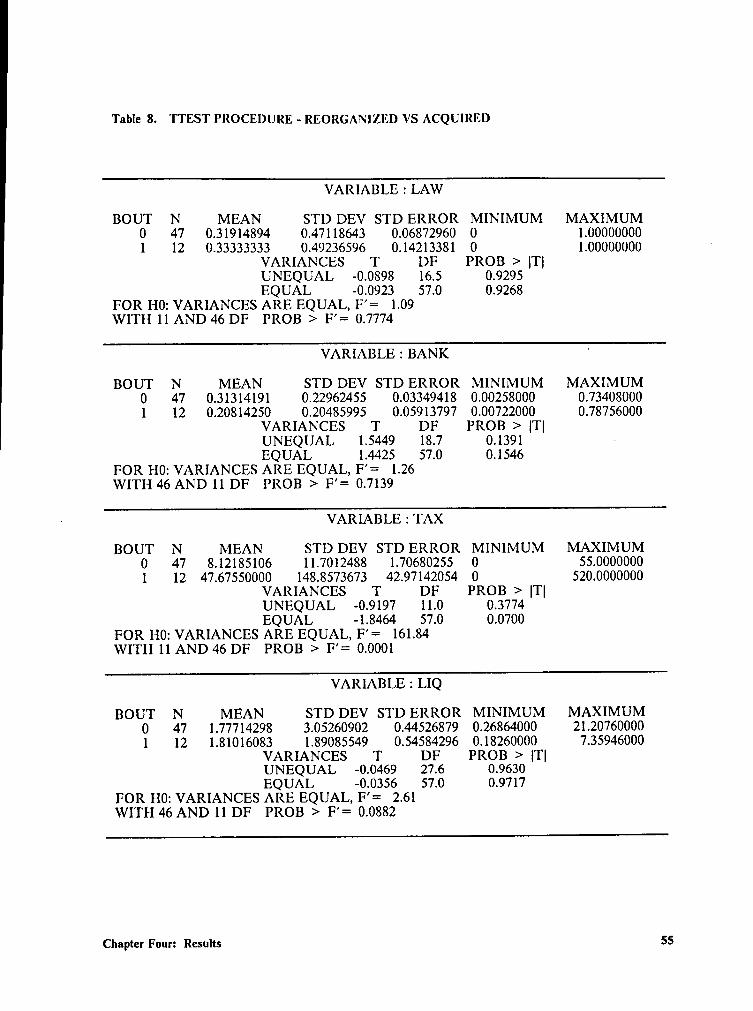
Table 8. TTEST PROCEDURE — REORGANIZED VS ACQUIRED
VARIABLE : LAW
BOUT N MEAN STI) DEV STD ERROR MINIMUM MAXIMUM0 47 0.31914894 0.47118643 0.06872960 0 1.000000001 12 0.33333333 0.49236596 0.14213381 0 1.00000000 '
VARIANCES T DF PROB > \T|UNEQUAL -0.0898 16.5 0.9295EQUAL -0.0923 57.0 0.9268
FOR H0: VARIANCES ARE EQUAL,F’=
1.09WITH 11 AND 46 DF PROB >
F’=0.7774
VARIABLE :
BANKBOUTN MEAN STD DEV STD ERROR MINIMUM MAXIMUM0 47 0.31314191 0.22962455 0.03349418 0.00258000 0.734080001 12 0.20814250 0.20485995 0.05913797 0.00722000 0.78756000
VARIANCES T DF PROB > [TlUNEQUAL 1.5449 18.7 0.1391 -EQUAL 1.4425 57.0 0.1546
FOR H0: VARIANCES ARE EQUAL, F’= 1.26WITH 46 AND 11 DF PROB > F’= 0.7139
- VARIABLE : TAX
BOUT N MEAN STD DEV STD ERROR MINIMUM MAXIMUM0 47 8.12185106 11.7012488 1.70680255 0 55.00000001 12 47.6755000O 148.8573673 42.97142054 0 $20.0000000
VARIANCES T DF PROB > |T|UNEQUAL -0.9197 11.0 0.3774EQUAL -1.8464 57.0 0.0700
FOR H0: VARIANCES ARE EQUAL,F’=
161.84WITH 11 AND 46 DF PROB >
F’=0.0001
VARIABLE : LIQ
BOUT N MEAN STD DEV STD ERROR MINIMUM MAXIMUM0 47 1.77714298 3.05260902 0.44526879 0.26864000 21.20760000l 12 1.81016083 1.89085549 0.54584296 0.18260000 7.35946000
VARIANCES T DF PROB > lT|UNEQUAL -0.0469 27.6 0.9630 „EQUAL -0.0356 57.0 0.9717
FOR H0: VARIANCES ARE EQUAL, F’= 2.61WITH 46 AND 11 DF PROB > F’= 0.0882
Chapter Four: Results 55
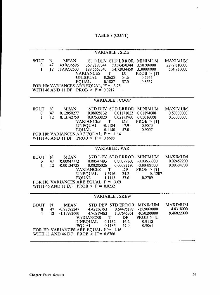
TABLE 8 (CONT)
VARIABLE : SIZE
BOUT N MEAN STD DEV STD ERROR MINIMUM MAXIMUM0 47 140.0236596 367.2197344 $3.56450344 3.50100000 2297.8100001 12 I19.9232500 189.$568340 $4.72034458 3.30000000 554.735000 _
VARIANCES T DF PROB > [TlUNEQUAL 0.2625 34.6 0.7945EQUAL 0.1827 57.0 0.8557
FOR H0: VARIANCES ARE EQUAL,F’=
3.75WITH 46 AND 11 DF PROB >
F’=0.0217
‘
VARIABLE : COUP
BOUT N MEAN STD DEV STD ERROR MINIMUM MAXIMUM0 47 0.12850277 0.08028132 0.01171023 0.01894000 0.500000001 12 0.13142750 0.07530820 0.02173960 0.05016000 0.33000000
VARIANCES T DF PROB > [TlUNEQUAL -0.1184 17.9 0.9070EQUAL -0.1140 57.0 0.9097
FOR H0: VARIANCES ARE EQUAL,F’=
1.14WITH 46 AND 11 DF PROB >
F’=0.8688
VARIABLE : VAR
BOUT N MEAN STD DEV STD ERROR MINIMUM MAXIMUM0 47 0.00047772 0.00547493 0.00079860 -0.00633000 0.024522001 12 -0.00134725 0.00285026 0.00082280 -0.00488000 0.00304700
VARIANCES T DF PROB >[TlUNEQUAL1.5916 34.2 0. 1207
EQUAL 1.1118 57.0 0.2709FOR H0: VARIANCES ARE EQUAL, F’= 3.69WITH 46 AND 11 DF PROB > F’= 0.0232
VARIABLE : SKEW
BOUT N MEAN STD DEV STD ERROR MINIMUM MAXIMUM0 47 -0.98582247 4.42156793 0.64495197 -15.9060000 14.83180001 12 -1.15792000 4.76817483 1.37645351 -9.50299000 9.46822000
VARIANCES T DF PROB > [TlUNEQUAL 0.1132 16.2 0.9113EQUAL 0.1185 57.0 0.9061
FOR H0: VARIANCES ARE EQUAL, F’= 1.16WITH I1 AND 46 DF PROB > F’= 0.6766
Chapter Four: Results 56
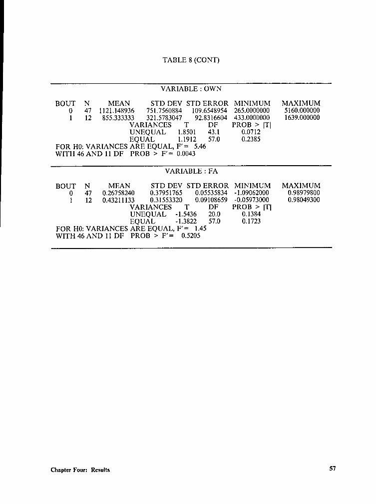
TABLE 8 (CONT)
VARIABLE : OWN
BOUT N MEAN STD DEV STD ERROR MINIMUM MAXIMUM0 47 1l21.148936 751.7560884 l09.6548954 265.0000000 $160.0000001 12 855.333333 321.$78}047 92.8316604 43}.0000000 1639.000000
VARIANCES T DF PROB > |T|UNEQUAL 1.8501 4}.1 0.0712EQUAL 1.1912 57.0 0.2385
FOR H0: VARIANCES ARE EQUAL, F’= 5.46WITH 46 AND 11 DF PROB > F’= 0.004}
VARIABLE : FA
BOUT N MEAN STD DEV STD ERROR MINIMUM MAXIMUM0 47 0.26758240 0.37951765 0.05535834 -1.09062000 0.989798001 12 0.43211133 0.31553320 0.09108659 -0.05973000 0.98049300
VARIANCES T DF PROB > |T|UNEQUAL -1.5436 20.0 0.1384EQUAL -1.3822 57.0 0.1723
FOR H0: VARIANCES ARE EQUAL, F’= 1.45WITH 46 AND 11 DF PROB >
F’=0.5205
Chapter Four: Results 57
Reorgauized versus Liquidated
Table 9 presents the results of the logit analysis for the 47 reorganized and 42 liq-
uidated firms. According to the chi-square statistic of 26.77 (ll df) the model is signif-
icant at the ot = 0.005 level. The variance of returns variable (VAR) is significant at the
ot = 0.0035 level and has a positive BETA, supporting Golbe’s hypothesis that liqui-
dation is less likely to occur as variance of returns is increased. The coupon rate variable
(COUP) is significant at the ot = 0.0604 level also with a positive BETA, providing fur-
ther rebuttal of Bulow and Shoven's argument that the greater the amount of funds re-
quired to be of banklenders, the more likely the firm will be liquidated. A more
reasonable argument is that the greater the potential loss to the existing bondholders,
the more likely the firm will be continued in some form. ·
The skewness of returns variable (SKEW) is significant at the oz = 0.0136 level and
has a negative BETA, which contradicts Golbe’s hypothesis that the greater the poten-”
tial return with a limited downside return, the more likely a firm will be continued. This
is not too surprising because as the owners make riskier investments, they reduce the
value of the existing debt. The riskier a firm's investments become, the more likely the
existing creditors are to force liquidation rather than sustain a transfer of wealth to the
stockholders. Another possible explanation for this finding is that the variance and
skewness variables are highly correlated. However, the correlation coeflicient between
these two variables for the reorganized and liquidated groups is only 0.1035.
The model is also estimated with the coupon rate variable adjusted for the level of
interest rates at the time of filing. As Table 10 reveals, the interest rate variable (INT)
Chapter Four: Results S8
once again drops in significance. For the Baa adjustment, INT is significant only at the
tx = 0.1136 levcl and for the prime rate adjustment t11e significance is at the ot = 0.0840
level.
Interestingly, the tax loss caryovcrs variable (TAX) enters the model at a signif-
icance level of ot = 0.0874 for the Baa adjustment and a significance level of a = 0.0946
level for the prime rate adjustment both with a negative coefficient. The negative coefl
ficient is opposite ofwhat was hypothesized. While financial theory recognizes that tax
loss carryovers can be recognized only if the firm continues either through reorganiza-
tion or acquisition, it is also possible that this variable is proxying for the extent of fi-
nancial distress which exists at the time of bankruptcy filing. That is, a firm with large
tax loss carryovers may in fact be the one for which liquidation is the highest value cre-
ating option.
The t-tests in Table ll find that the coupon interest (COUP) and variance of re-
turns (VAR) variables have means significantly different when grouped by reorganized
versus liquidated outcomes. The coupon interest rate for the reorganized firms has a
mean of 12.85% while the mean for the liquidated group is 9.92%. These means are
significantly different at the ot = 0.0121 level. The variance of returns variable averaged
0.00048 for the reorganized firms and -0.00187 for the liquidated firms and are signif-
icantly different at the ot = 0.0183 level. This further supports the findings of the logit
analysis that the liquidated outcome is significantly different from the reorganized out-
come for firms which have filed bankruptcy.
Chapter Four: Results 59
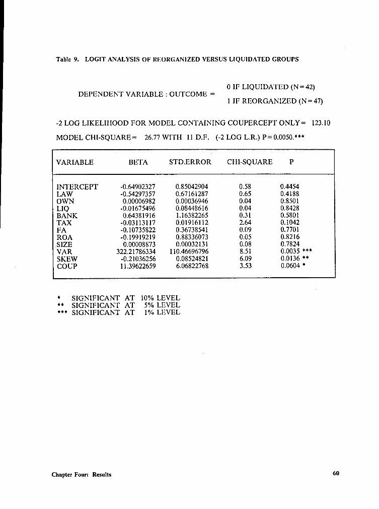
Table 9. LOGIT ANALYSIS OF REORGANIZED VERSUS LIQUIDATED GROUPS
0 IF LIQUIDATED (N=42)DEPENDENT VARIABLE : OUTCOME =
1 IF REORGANIZED (N=47)
-2 LOG LIKELIIIOOD FOR MODEL CONTAINING COUPERCEPT ONLY= 123.10
MODEL CHI-SQUARE= 26.77 WITH 11 D.F. (-2 LOG L.R.) P= 0.0050.***
VARIABLE BETA STD.ERROR CHI-SQUARE P
INTERCEPT -0.64902327 0.85042904 0.58 0.4454LAW -0.54297357 0.67161287 0.65 0.4188OWN 0.00006982 0.00036946 0.04 0.8501LIQ -0.01675496 0.08448616 0.04 0.8428BANK 0.64381916 1.16382265 0.31 0.5801TAX -003113117 0.01916112 2.64 0.1042FA -0.l0735822 0.36738541 0.09 0.7701ROA -0.19919219 0.88336073 0.05 0.8216SIZE 0.00008873 0.00032131 0.08 0.7824VAR 322.21786334 IIO.46696796 8.51 0.0035 ***SKEW ·0.21036256 0.08524821 6.09 0.0136 **COUP 11.39622659 6.06822768 3.53 0.0604 *
* SIGNIFICANT AT 10% LEVEL** SIGNIFICANT AT 5% LEVEL*** SIGNIFICANT AT 1% LEVEL
Chapter Four: Results 60
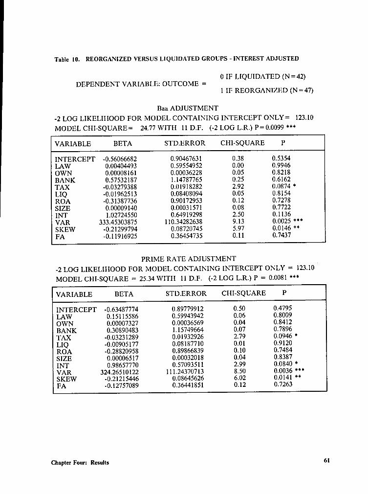
Table l0. REORGANIZED VERSUS LIQUIDATED GROUPS - INTEREST ADJUSTED
0 IF LIQUIDATED (N=42)DEPENDENT VARIABLE: OUTCOME =
1 IF REORGANIZED (N=47)
Baa ADJUSTMENT-2 LOG LIKELIIIOOD FOR MODEL CONTAINING INTERCEPT ONLY= 123.10
MODEL CHI-SQUARE= 24.77 WITI·I 11 D.F. (-2 LOG L.R.) P= 0.0099 ***
VARIABLE BETA STD.ERROR CH1·SQUARE P
INTERCEPT ·0.56066682 0.90467631 0.38 0.5354LAW 0.00404493 0.59554952 0.00 0.9946OWN 0.00008161 0.00036228 0.05 0.8218BANK 0.57532187 1.14787765 0.25 0.6162TAX -0.03279388 0.01918282 2.92 0.0874 *LIQ -0.01962513 0.08408094 0.05 0.8154ROA ·0.31387736 0.90172953 0.12 0.7278SIZE 0.00009140 0.00031571 0.08 0.7722INT 1.02724550 0.64919298 2.50 0.1136VAR 333.45303875 110.34282638 9.13 0.0025 ***SKEW -0.21299794 0.08720745 5.97 0.0146 **FA -0.11916925 0.36454735 0.11 0.7437
PRIME RATE ADJUSTMENT _-2 LOG LIKELIHOOD FOR MODEL CONTAINING INTERCEPT ONLY = 123.10
MODEL CHI—SQUARE = 25.34 WITI·I 11 D.F. (-2 LOG L.R.) P = 0.0081 ***
VARIABLE BETA STD.ERROR CHI-SQUARE P
INTERCEPT -0.63487774 0.89779912 0.50 0.4795LAW 0.15115586 0.59943942 0.06 0.8009OWN 0.00007327 0.00036569 0.04 0.8412BANK 0.30890483 1.15749664 0.07 0.7896TAX -0.03231289 0.01932926 2.79 0.0946 *LIQ -0.00905177 0.08187710 0.01 0.9120ROA -0.28820958 0.89866839 0.10 0.7484SIZE 0.00006517 0.00032018 0.04 0.8387INT 0.98657770 0.57093511 2.99 0.0840 *VAR 324.26510122 111.243707l3 8.50 0.0036 ***SKEW -0.21215446 0.08645626 6.02 0.0141 **FA -0.12757089 0.36441851 0.12 0.7263
Chapter Four: Results 61
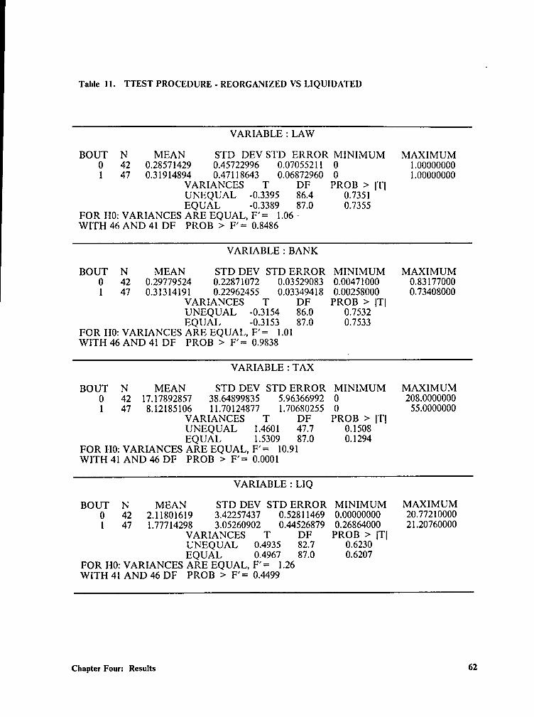
Table ll. TTEST PROCEDURE - REORGANIZED VS LIQUIDATED
VARIABLE : LAW
BOUT N MEAN STD DEV STD ERROR MINIMUM MAXIMUM0 42 0.28571429 0.45722996 0.07055211 0 1.000000001 47 0.31914894 0.47118643 0.06872960 0 1.00000000
VARIANCES T DF PROB > |T|UNEQUAL -0.3395 86.4 0.7351EQUAL -0.3389 87.0 0.7355
FOR H0: VARIANCES ARE EQUAL,F’=
1.06 ·~WITH 46 AND 41 DF PROB > F’= 0.8486
VARIABLE : BANK
BOUT N MEAN STD DEV STD ERROR MINIMUM MAXIMUM0 42 0.29779524 0.22871072 0.03529083 0.00471000 0.831770001 47 0.31314191 0.22962455 0.03349418 0.00258000 0.73408000
VARIANCES T DF PROB > |T|UNEQUAL -0.3154 86.0 0.7532EQUAL -0.3153 87.0 0.7533
FOR IIO: VARIANCES ARE EQUAL,F’=
1.01WITH 46 AND 41 DF PROB > F’= 0.9838
VARIABLE : TAX
BOUT N MEAN STD DEV STD ERROR MINIMUM MAXIMUM0 42 17.17892857 38.64899835 5.96366992 0 208.00000001 47 8.12185106 11.70124877 1.70680255 0 55.0000000
VARIANCES T DF PROB > |T|UNEQUAL 1.4601 47.7 0.1508EQUAL 1.5309 87.0 0.1294
FOR H0: VARIANCES ARE EQUAL,F’=
10.91WITH 41 AND 46 DF PROB > F’= 0.0001
VARIABLE : LIQ
BOUT N MEAN STD DEV STD ERROR MINIMUM MAXIMUM0 42 2.11801619 3.42257437 0.52811469 0.00000000 20.7721000O1 47 1.77714298 3.05260902 0.44526879 0.26864000 21.2076000O
VARIANCES T DF PROB > |T|UNEQUAL 0.4935 82.7 0.6230EQUAL 0.4967 87.0 0.6207
FOR H0: VARIANCES ARE EQUAL,F’=
1.26WITH 41 AND 46 DF PROB >
F’=0.4499
Chapter Four: Results 62
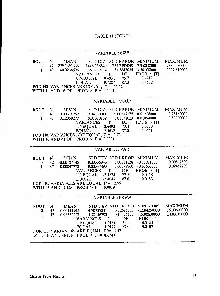
TABLE I1 (CONT)
VARIABLE : SIZE
BOUT N MEAN STD DEV STD ERROR MINIMUM MAXIMUM0 42 299.1493333 1446.75864O 223.2397048 2.95800000 9382.68000O1 47 140.0236596 367.219734 53.5645034 3.50100000 2297.810000
VARIANCES T DF PROB > |T|UNEQUAL 0.6931 45.7 0.4917EQUAL 0.7287 87.0 0.4682
FOR H0: VARIANCES ARE EQUAL,F’=
15.52WITH 41 AND 46 DF PROB > F’= 0.0001
VARIABLE 2 COUP
BOUT N MEAN STD DEV STD ERROR MINIMUM MAXIMUM0 42 0.09318262 0.04130011 0.00637275 0.01228000 0.231600001 47 0.12850277 0.08028132 0.01171023 0.01894000 0.50000000
VARIANCES T DF PROB > |T|UNEQUAL -2.6493 70.4 0.0100EQUAL -2.5632 87.0 0.0121
FOR H0: VARIANCES ARE EQUAL,F’=
3.78WITH 46 AND 41 DF PROB >
F’=0.0001
VARIABLE : VAR
BOUT N MEAN STD DEV STD ERROR MINIMUM MAXIMUM0 42 -0.00187145 0.00335946 0.00051838 -0.00971000 0.008928001 47 0.00047772 0.00547493 0.00079860 —0.00633000 0.02452200
VARIANCES T DF PROB > |T|UNEQUAL -2.4674 77.5 0.0158EQUAL -2.4047 87.0 0.0183
FOR H0: VARIANCES ARE EQUAL, F’= 2.66WITH 46 AND 41 DF PROB >
F’=0.0019
VARIABLE 2 SKEW
BOUT N MEAN STD DEV STD ERROR MINIMUM MAXIMUM0 42 0.00144945 4.70989341 0.72675233 -12.84250000 15.906000001 47 -0.98582247 4.42156793 0.64495197 -15.90600000 14.8318000O
VARIANCES T DF PROB > |T|UNEQUAL 1.0161 84.4 0.3125EQUAL 1.0197 87.0 0.3107
FOR H0: VARIANCES ARE EQUAL,F’=
1.13WITH 41 AND 46 DF PROB >
F’=0.6747
Chapter Four: Rcsults 63
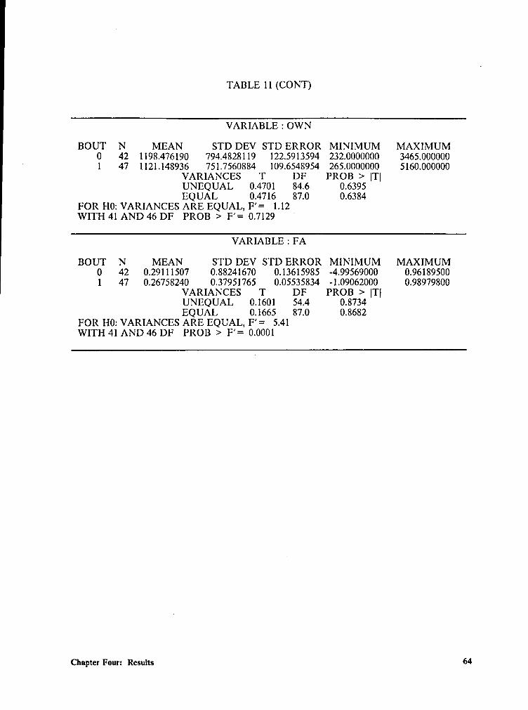
TABLE 11 (CONT)
VARIABLE : OWN
BOUT N MEAN STD DEV STD ERROR MINIMUM MAXIMUM0 42 1198.47619O 794.4828119 122.$913594 232.0000000 3465.000000l 47 1121.148936 751.7560884 109.6548954 2650000000 $160.000000
VARIANCES T DF PROB > |T|UNEQUAL 0.4701 84.6 0.6395EQUAL 0.4716 87.0 0.6384
FOR H0: VARIANCES ARE EQUAL, F’= 1.12WITI·1 41 AND 46 DF PROB > F’=
0.7129VARIABLE : FA
BOUT N MEAN STD DEV STD ERROR MINIMUM MAXIMUM0 42 0.29111507 0.88241670 0.13615985 -4.99569000 0.961895001 47 0.26758240 0.37951765 0.05535834 -1.09062000 0.98979800
VARIANCES T DF PROB > |T|UNEQUAL 0.1601 54.4 0.8734EQUAL 0.1665 87.0 0.8682
FOR H0: VARIANCES ARE EQUAL, F’= 5.41WITH 41 AND 46 DF PROB > F’= 0.0001
Chapter Four: Results 64
Coutiuued versus Liquidated
When grouping acquired firms with the reorganized firms and performing the logit
analysis on the 59 "continued" firms versus the 42 liquidated firms, the results, presented
in Table 12 are in agreement with those in Table 9. The model is signilicant at the
ol = 0.013 level and the coupon rate (COUP), variance of returns (VAR) and the
skewness of returns (SKEW) variables are signilicant and their signs remain the same.
The coupon rate is signilicant at the tx = 0.0153 level, the variance of returns is signif-
icant at the ot = 0.0097 level and the skewness of returns is significant at the
“oz = 0.0182 level.
When the coupon rate is adjusted for the level of interest rates, (see Table 13) the
signs of the variables remains the same. The Baa adjustment leads to a model signif-
icance of oz = 0.0381 with the interest rate variable (INT) significant at the ot = 0.0490
level, the variance of returns variable (VAR) significant at the tx = 0.0073 level, and the
skewness of returns (SKEW) significant at the ot = 0.0195 level. When the prime rate
is used for the adjustment the model is signilicant at the tz = 0.0259 with the interest rate
variable (INT) signilicant at the tx = 0.0265 level, the variance of returns variable (VAR)
signilicant at the ot = 0.0107 level, and the skewness of returns (SKEW) significant at
the oz = 0.0196 level.
Overall, the model is statistically significant in distinguishing between liquidated
and reorganized firms. Furthermore, the variance of returns variable is significant and
has the correct sign. The skewness and the coupon rate variables are also signilicant but
Chapter Four: Results 65
have the opposite sign of that predicted by theory as above. These results suggest thatU
additional research is needed to understand this finding.
Eßect of the Law Change
In all of the above logit analyses, the dummy variable (DL) used to indicate a shift
in the data due to the change in the law was found to be insignificant. The results of the
logit model to test for interactive effects are presented in Table 14. The overall model
is signilicant at the ot = 0.0299 level. The coupon interest rate (COUP) is significant at
the cz = 0.0524 level, the variance of returns (VAR) is signiticant at the ot = 0.0016 level
and skewness of returns (SKEW) are significant at the oz = 0.0089 level. These variables
all have the same sign as in the previous continued versus liquidated analysis.
The only interactive variable found to be significant is the the one associated with
the variance of returns variable. The interactive variable (LVAR) represented by the
product of the dummy law variable and the variance of returns variable is significant at
the ot = 0.0245 level with a negative BETA. Tables l4.a. and 14.b. show that after ad-
justing for the interest rate proxy, the model drops slightly in signilicance to
ot = 0.0751 (Baa) and ot = 0.0703 (Prime) levels. The signilicant variables remain sig-
nificant and with the same sign. The effect suggested by these results is that the law
change works to reverse the effect of the variance of returns variable. That is that the
interactive effect of the law dummy variable on the variance of returns variable is to re-
duce the likelihood of continuance after the law change.
Chapter Four: Results 66

Table 12. LOGIT ANALYSIS OF CONTINUED VERSUS LIQUIDATED GROUPS
0 IF LIQUIDATED (N= 42)DEPENDENT VARIABLE : OUTCOME =
1 IF CONTINUED (N= 59)
-2 LOG L1KELI1·1OOD FOR MODEL CONTAINING COUPERCEPT ONLY= 137.14
MODEL CHI-SQUARE= 23.95 WITH 11 D.F. (-2 LOG L.R.) P= 0.0130**
VARIABLE BETA STD.ERROR CHI-SQUARE P
INTERCEPT ·0.40720685 0.82421343 0.24 0.6213LAW ·0.47881487 0.62361480 0.59 0.4426OWN -0.00029219 0.00037177 0.62 0.4319LIO -0.02454926 0.08099979 0.09 0.7618
BANK 0.19785481 1.11565872 0.03 0.8592TAX -0.00436269 0.00436496 1.00 0.3176FA -0.07893037 0.36373297 0.05 0.8282ROA 0.29055240 0.77694015 0.14 0.7084SIZE -0.00009298 0.00028342 0.11 0.7429VAR 260.23873112 100.56872839 6.70 0.0097 "'**SKEW -0.16481514 0.06980587 5.57 0.0182 **COUP 14.5502852O 6.00192657 5.88 0.0153 **
* SIGNIFICANT AT 10% LEVEL** SIGNIFICANT AT 5% LEVEL*** SIGNIFICANT AT 1% LEVEL
Chaptcr Four: Results67
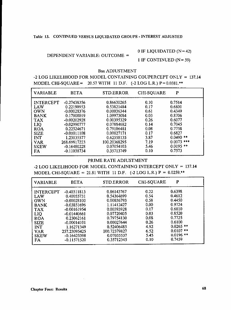
Table 13. CONTINUED VERSUS LIQUIDATED GROUPS - INTEREST ADJUSTED
0 IF LIQUIDATED (N= 42)DEPENDENT VARIABLE: OUTCOME =
1 IF CONTINUED (N= 59)
Baa ADJUSTMENT-2 LOG LIKELIHOOD FOR MODEL CONTAINING COUPERCEPT ONLY = 137.14MODEL CHI—SQUARE= 20.57 WITH 11 D.F. (-2 LOG L.R.) P= 0.0381.**
VARIABLE BETA STD.ERROR CHI-SQUARE P
INTERCEPT -0.27438356 0.86630265 0.10 0.7514LAW 0.22190953 0.53821484 0.17 0.6801OWN -0.00028376 0.00036344 0.61 0.4349BANK 0.17908019 1.09973084 0.03 0.8706TAX ·0.00202928 0.00395329 0.26 0.6077LIQ -0.02990777 0.07884682 0.14 0.7045ROA 0.22524671 0.79106481 0.08 0.7758SIZE -0.00011108 0.00027171 0.17 0.6827INT 1.23135577 0.62558135 3.87 0.0490 **VAR 268.69817223 I00.20368295 7.19 0.0073 ***SKEW -0.16480228 0.07054103 5.46 0.0195 **FA -O.11038734 0.35713749 0.10 0.7573
PRIME RATE ADJUSTMENT-2 LOG LIKELIHOOD FOR MODEL CONTAINING INTERCEPT ONLY = 137.14MODEL CHI-SQUARE = 21.81 WITH 11 D.F. (-2 LOG L.R.) P = 0.0259.**
VARIABLE BETA STD.ERROR CHI-SQUARE P
INTERCEPT -0.40311813 0.86143767 0.22 0.6398LAW 0.40055731 0.54364699 0.54 0.4612OWN -0.0002810O 0.00036793 0.58 0.4450BANK -0.03851696 1.11412427 0.00 0.9724TAX -0.00161954 0.00393928 0.17 0.6810LIQ -0.0144066l 0.07720405 0.03 0.8520ROA 0.23062161 0.79754130 0.08 0.7725SIZE -0.00014101 0.00027644 0.26 0.6100INT 1.16271349 0.52406485 4.92 0.0265 **VAR Z57.23095425 l00.72379827 6.52 0.0107 **SKEW -0.16425398 0.07035537 5.45 0.0196 **FA -0.11571520 0.35712345 0.10 0.7459
Chapter Four: Results 68
The t-tests in Table 15 show that the means of the ownership concentration_
(OWN), size (SIZE), coupon interest rate (COUP), and free assets (FA) variables are
all significantly different across the law change. The means of the adjusted interest rates
are not significant, however. These results indicate that the law change may have af-
fected concentration of ownership, size, and free assets. The size and free assets results
may be due to two very large firms filing for bankruptcy after the law change creating
an outlier effect.I
The results of these analyses of the effect of law change are contradictory and in-
conclusive. A possible explanation of these results is that the judicial system enacted
by the 1978 Reform Act was not fully operationalized until 1984. This suggests further
research is in order to determine whether the Reform Act of 1978 had any significant
effect on the outcome of firms which have filed for bankruptcy.
Chapter Four-: Results 69
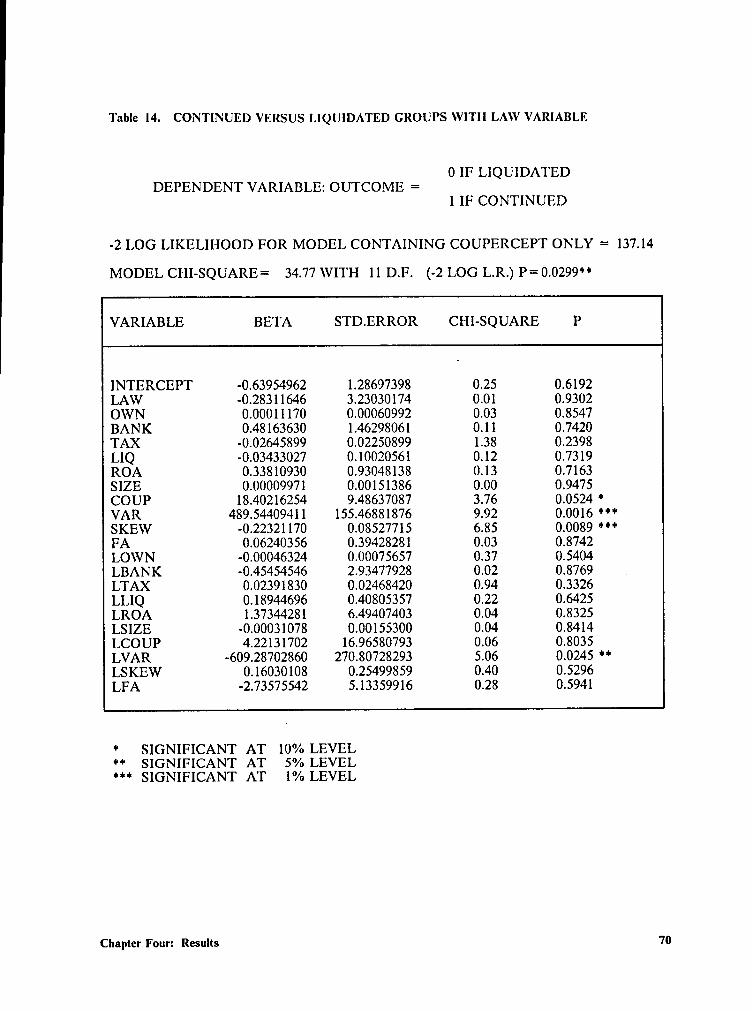
'1‘able I4. CONTINUED VERSUS LIQUIDATED GROUPS WITII LAW VARIABLE
0 IF LIQUIDATEDDEPENDENT VARIABLE: OUTCOME =
1 IF CONTINUED
-2 LOG LIKELIHOOD FOR MODEL CONTAINING COUPERCEPT ONLY = 137.14
MODEL CI·II-SQUARE= 34.77 WITH 11 D.F. (-2 LOG L.R.) P= 0.0299**
VARIABLE BETA STD.ERROR CHI-SQUARE P
INTERCEPT -0.63954962 1.28697398 0.25 0.6192LAW -0.28311646 3.23030174 0.01 0.9302OWN 0.00011170 0.00060992 0.03 0.8547BANK 0.48163630 1.46298061 0.11 0.7420TAX -0.02645899 0.02250899 1.38 0.2398LIQ -0.03433027 0.10020561 0.12 0.7319ROA 0.33810930 0.93048138 0.13 0.7163SIZE 0.00009971 0.00151386 0.00 0.9475COUP 18.40216254 9.48637087 3.76 0.0524 *VAR 489.544094Il 155.4688l876 9.92 0.0016 ***SKEW -0.22321170 0.08527715 6.85 0.0089 ***FA 0.06240356 0.39428281 0.03 0.8742LOWN -0.00046324 0.00075657 0.37 0.5404LBANK -0.45454546 2.93477928 0.02 0.8769 .LTAX 0.02391830 0.02468420 0.94 0.3326LLIQ 0.18944696 0.40805357 0.22 0.6425LROA 1.37344281 6.49407403 0.04 0.8325LSIZE —0.00031078 0.00155300 0.04 0.8414LCOUP 4.22131702 16.96580793 0.06 0.8035LVAR -609.28702860 Z70.80728293 5.06 0.0245 **LSKEW 0.16030108 0.25499859 0.40 0.5296LFA -2.73575542 5.13359916 0.28 0.5941
* SIGNIFICANT AT 10% LEVEL** SIGNIFICANT AT 5% LEVEL*** SIGNIFICANT AT 1% LEVEL
Chapter Four: Results 70
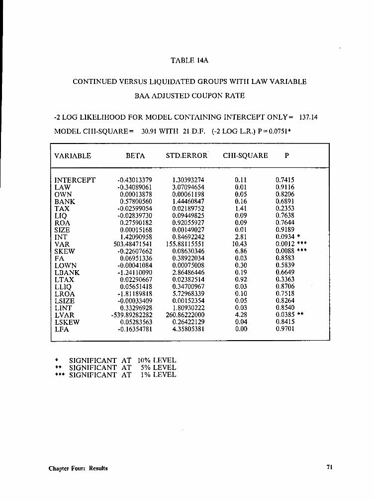
TABLE 14A
CONTINUED VERSUS LIQUIDATED GROUPS WITII LAW VARIABLE
BAA ADJUSTED COUPON RATE
-2 LOG LIKELIHOOD FOR MODEL CONTAINING INTERCEPT ONLY= 137.14
MODEL CHI-SQUARE= 30.91 WITH 21 D.F. (-2 LOG L.R.) P= 0.0751*
VARIABLE BETA STDERROR8 CHI-SQUARE P
INTERCEPT -0.43013379 1.30393274 0.11 0.7415LAW -0.3408906l 3.07094654 0.01 0.9116OWN 0.00013878 0.00061198 0.05 0.8206BANK 0.57800560 1.44460847 0.16 0.6891TAX -0.02599054 0.02189752 1.41 0.2353LIQ -0.02839730 0.09449825 0.09 0.7638ROA 0.27590182 0.92055927 0.09 0.7644SIZE 0.00015168 0.00149027 0.01 0.9189INT 1.42090958 0.84692242 2.81 0.0934 *VAR 503.48471541 155.88115551 10.43 0.0012 ***SKEW -0.22607662 0.08630346 6.86 0.0088 ***FA 0.06951336 0.38922034 0.03 0.8583LOWN -0.00041084 0.00075008 0.30 0.5839LBANK -1.24110090 2.86486446 0.19 0.6649LTAX 0.02290667 0.02382514 0.92 0.3363LLIQ 0.05651418 0.34700967 0.03 0.8706LROA -1.81189818 5.72968339 0.10 0.7518LSIZE -0.00033409 0.00152354 0.05 0.8264LINT 0.33296928 1.80930222 0.03 0.8540LVAR ·539.89282282 26086222000 4.28 0.0385 **LSKEW 0.05283563 0.26422129 0.04 0.8415LFA -0.16354781 4.35805381 0.00 0.9701
* SIGNIFICANT AT 10% LEVEL** SIGNIFICANT AT 5% LEVEL"'** SIGNIFICANT AT 1% LEVEL
Chaptcr Four: Rcsults 71
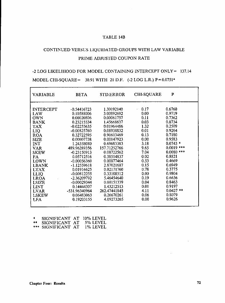
TABLE 14B
CONTINUED VERSUS LIQUIDATED GROUPS WITH LAW VARIABLE
PRIME ADJUSTED COUPON RATE
-2 LOG LIKELIHOOD FOR MODEL CONTAINING INTERCEPT ONLY= 137.14
MODEL CHI·SQUARE= 30.91 WITH 21 D.F. (-2 LOG L.R.) P=0.0751*
VARIABLE BETA STD.ERROR CHI-SQUARE P
INTERCEPT -0.54416723 1.30192140 · 0.17 0.6760LAW 0.10588006 3.00892692 0.00 0.9719OWN 0.00020806 0.00061757 0.11 0.7362BANK 0.23215534 1.45668637 0.03 0.8734TAX -0.02255635 0.01964486 1.32 0.2509LIQ -0.00825760 0.08938832 0.01 0.9264ROA 0.32722595 0.90603469 0.13 0.7180SIZE 0.00007738 0.00147923 0.00 0.9583INT 1.24358080 0.69683383 3.18 0.0743 *VAR 489.96289356 157.71252766 9.65 0.0019 ***SKEW ·0.23150913 0.08722562 7.04 0.0080 ***FA 0.05712516 0.38514837 0.02 0.8821LOWN -0.00056360 0.00077464 0.53 0.4669LBANK -1.l2559618 2.87021687 0.15 0.6949LTAX 0.01916625 0.02171760 0.78 0.3775LLIQ -0.0081225S 0.33108512 0.00 0.9804LROA . -2.36209792 5.46454640 0.19 0.6656LSIZE -0.00029344 0.00151339 0.04 0.8463LINT 0.14444307 1.43212513 0.01 0.9197LVAR -531.96340964 262.47441845 4.11 0.0427 **LSKEW 0.06483063 0.26670261 0.06 0.8079LFA 0.19203155 4.09273265 0.00 0.9626
* SIGNIFICANT AT 10% LEVEL** SIGNIFICANT AT 5% LEVEL*** SIGNIFICANT AT 1% LEVEL
Chapter Four: Results 72
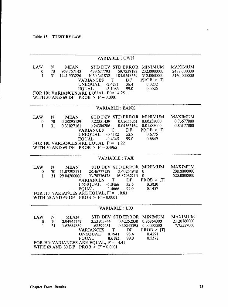
Table 15. TTEST BY LAW
VARIABLE : OWN
LAW N MEAN STD DEV STD ERROR MINIMUM MAXIMUM0 70 969.757143 499.677793 59.7229193 232.0000000 2487.0000001 31 144I.903226 1030.341832 185.0548559 312.0000000 $160.000000
VARIANCES T DF PROB > |T|UNEQUAL -2.4281 36.4 0.0202EQUAL -3.1083 99.0 0.0025
FOR H0: VARIANCES ARE EQUAL, F’= 4.25 —
WITH 30 AND 69 DF PROB > F’=0.0001
VARIABLE : BANK
LAW N MEAN STD DEV STD ERROR MINIMUM MAXIMUM0 70 0.28895129 0.22031439 0.02633261 0.00258000 0.735770001 31 0.31027161 0.24304206 0.04365164 0.01588000 0.83177000
VARIANCES T DF PROB > |T|UNEQUAL -0.4182 52.8 0.6775EQUAL -0.4345 99.0 0.6649
FOR H0: VARIANCES ARE EQUAL, F’= 1.22WITH 30 AND 69 DF PROB > F’=0.4965
VARIABLE : TAX
LAW N MEAN STD DEV STD ERROR MINIMUM MAXIMUM0 70 11.0720857l 28.46777139 3.40254948 0 Z08.00000001 31 Z9.04200000 93.70336478 16.82962113 0 $20.0000000
VARIANCES T DF PROB > |T|UNEQUAL -1.0466 32.5 0.3030EQUAL -1.4666 99.0 0.1457
FOR H0: VARIANCES ARE EQUAL, F’= 10.83WITH 30 AND 69 DF PROB > F’= 0.0001
VARIABLE 2 LIQ
LAW N MEAN STD DEV STD ERROR MINIMUM MAXIMUM0 70 2.04945757 3.53505844 0.42252030 0.26864000 21.207600001 31 1.63684839 1.68399231 0.30245395 0.00000000 7.75557000
VARIANCES T DF PROB > |T|UNEQUAL 0.7941 98.4 0.4291EQUAL 0.6183 99.0 0.5378
FOR H0: VARIANCES ARE EQUAL, F’= 4.41WITH 69 AND 30 DF PROB > F’= 0.0001
Chapter Four: Results 73
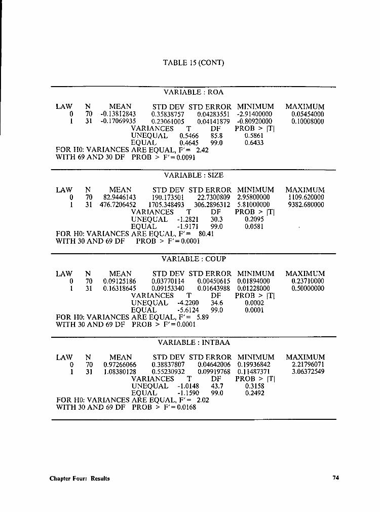
TABLE 15 (CONT)
VARIABLE : ROA
LAW N MEAN STD DEV STD ERROR MINIMUM MAXIMUM0 70 -0.13812843 0.35838757 0.04283551 -2.9140000O 0.054540001 31 -0.1706993S 0.23061005 0.04141879 -0.80920000 0.10008000
VARIANCES T DF PROB > |T|UNEQUAL 0.5466 85.8 0.5861EQUAL 0.4645 99.0 0.6433
FOR H0: VARIANCES ARE EQUAL, F’= 2.42WITH 69 AND 30 DF PROB > F’=0.0091
VARIABLE : SIZE
LAW N MEAN STD DEV STD ERROR MINIMUM MAXIMUM0 70 82.9446143 190.173501 22.7300809 2.95800000 1109.6200001 31 476.7206452 l705.348493 306.2896312 5.81000000 9382.68000O
VARIANCES T DF PROB > |T|UNEQUAL -1.2821 30.3 0.2095EQUAL -1.9171 99.0 0.0581 -
FOR H0: VARIANCES ARE EQUAL,F’=
80.41WITH 30 AND 69 DF PROB > F’=0.0001
VARIABLE : COUP
LAW N MEAN STD DEV STD ERROR MINIMUM MAXIMUM0 70 0.09125186 0.03770114 0.00450615 0.01894000 0.237100001 31 0.16318645 0.09153340 0.01643988 0.01228000 0.50000000
VARIANCES T DF PROB > |T|UNEQUAL -4.2200 34.6 0.0002EQUAL -5.6124 99.0 0.0001
FOR H0: VARIANCES ARE EQUAL,F’=
5.89WITH 30 AND 69 DF PROB > F’=0.0001
VARIABLE : INTBAA
LAW N MEAN STD DEV STD ERROR MINIMUM MAXIMUM0 70 0.97266066 0.38837807 0.04642006 0.19936842 2.217960711 31 1.08380128 0.55230932 0.09919768 0.11487371 3.06372549
VARIANCES T DF PROB > |T|UNEQUAL -1.0148 43.7 0.3158EQUAL -1.1590 99.0 0.2492
FOR H0: VARIANCES ARE EQUAL,F’=
2.02WITH 30 AND 69 DF PROB >
F’=0.0168
Chapter Four: Results 74
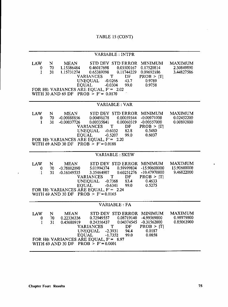
TABLE 15 (CONT)
VARIABLE : INTPR
LAW N MEAN STD DEV STD ERROR MINIMUM MAXIMUM0 70 1.15386484 0.46017698 0.05500167 0.17520814 2.308498901 31 1.15731274 0.65389098 0.11744229 0.09692186 3.44827586
VARIANCES T DF PROB > [TlUNEQUAL -0.0266 43.7 0.9789EQUAL -0.0304 99.0 0.9758
FOR H0: VARIANCES ARE EQUAL, F’= 2.02WITH 30 AND 69 DF PROB >
F’=0.0170
F"
VARIABLE : VAR
LAW N MEAN STD DEV STD ERROR MINIMUM MAXIMUM0 70 -0.00088856 0.00498178 0.00059544 -0.00971000 0.024522001 31 -0.00037726 0.00335841 0.00060319 -0.00557000 0.00892800
VARIANCES T DF PROB > [TlUNEQUAL -0.6032 82.8 0.5480EQUAL -0.5207 99.0 0.6037
FOR H0: VARIANCES ARE EQUAL, F’= 2.20WITH 69 AND 30 DF PROB > F’=0.0188
VARIABLE : SKEW
LAW N MEAN STD DEV STD ERROR MINIMUM MAXIMUM .0 70 -0.7880209O 5.01994374 0.59999804 -15.90600000 15.9060000O
· 1 3l -0.16149535 3.35464907 0.60251276 -10.47970000 9.46822000VARIANCES T DF PROB > [Tl
V
UNEQUAL -0.7368 83.4 0.4633EQUAL -0.6341 99.0 0.5275
FOR H0: VARIANCES ARE EQUAL,F’=
2.24 '
WITH 69 AND 30 DF PROB > F’=0.0165
VARIABLE : FA
LAW N MEAN STD DEV STD ERROR MINIMUM MAXIMUM0 70 0.22336336 0.72949557 0.08719140 -4.99569000 0.989798001 31 0.45680919 0.24356437 0.04374545 -0.31562000 0.85063900
VARIANCES T DF PROB > [TlUNEQUAL -2.3931 94.4 0.0187EQUAL -1.7352 99.0 0.0858
FOR H0: VARIANCES ARE EQUAL,F’=
8.97WITH 69 AND 30 DF PROB > F’=0.0001
Chapter Four: Results 75
Chapter Five: Summary and Directions for Future
Research
Introduction‘
In this chapter, the results and main conclusions are reviewed and summarized and
suggested directions for future research are presented. The first section summarizes the
study and highlights the main contributions and the second section points out the limi-
tations of the study and suggests possible extensions and improvements.
Chapter Five: Summary and Directions for Future Research 76
Sllllllllllljf
The present study develops and estimates a model to statistically distinguish among
liquidated, acquired, and reorganized firms which initially filed bankruptcy. The results
of the study revcal that the model clearly distinguishes between liquidated and reorgan-
ized firms and to some extent between liquidated. and acquired firms. In contrast to a
prior study which categorizes acquired firms as liquidated, the present study demon-
strates that if they are to be assigned to either other group, it should be the reorganized
firms.
When analyzing acquired firms versus liquidated firms the variables that demon-
strate statistically significant influence on the outcomes between the groups are owner-
ship concentration and coupon interest rate. The ownership concentration variable is
as hypothesized from an agency viewpoint. The coupon rate effect is opposite to that
expected by theory and is adjusted for current interest rates. The significance of the
coupon rate effect is reduced and the variance of returns becomes significant with the
hypothesized sign. The results of the analysis of the acquired firms versus the reorgan-
ized firms found no statistically significant difference between the groups. The t-tests for
differences between the means of the variables separated by groups are in agreement
with the logit analyses. The results of these analyses suggest that prior studies which
grouped acquired firms with liquidated firms were doing so inappropriately. Further,
studies which ignored acquired firms were unnecessarily reducing their sample size.
When grouping the acquired firms with the reorganized firms into an intuitively
appealing "continued" group, the variables that statistically influence the outcomes
Chapter Five: Summary and Directions for Future Research 77
among the groups are variance of security returns, the average coupon rate, and
skewness of security returns. The variance of returns variable has the hypothesized sign.
The skewness of returns and the average coupon rate have signs opposite to those hy-
pothesized. The average coupon rate variable becomes insignificant when adjusted for
current interest rates, suggesting that the coupon rate was proxying for these rates. The
skewness of returns variable may be misspecified due to omitted relevant explanatory
variables. Further research is needed to understand this finding. It is interesting to note
that the variables significantly influencing the outcome of a bankruptcy filing are market
variables rather than financial statement variables. This suggests that the market has
assimilated the appropriate information in ascertaining the outcome of firms which have
filed for bankruptcy.
The binary variable representing the change in the bankruptcy code (effective in
1979) was not statistically significant in any of the estimated models. The results of the
interactive model suggests that only the variance of returns variable interacts with the
law change dummy variable. One possible explanation for the insignificance of this fre-
quently discussed and presumably important change in the bankruptcy law is that the
judicial system enacted by the 1978 law to deal with bankruptcy cases was not fully
operationalized until 1984. The T-Tests found significant differences between means
across the law change for the ownership concentration, size, coupon interest rate, and
free assets variables. The results of the two analyses are contradictory and inconclusive.
Chapter Five: Summary and Directions for Future Research 78

'
Limitations and Future ResearchThis dissertation, as any other study of the problems ofbankruptcy, must deal with
limited data. The number of bankrupt firms of sufficient size and/or importance to be
included in the major data bases is limited. Further, once the firms that are included in
the data bases become financially distressed, the filing of information becomes sporadic
and untimely. A continuing buildup of a database of bankrupt firms will allow for
continued research in the areas covered in this study.
The results of the logit analysis and the T-Tests for the effect of the law change
are contradictory and inconclusive. This suggests that additional study is required. As
data becomes available for firms which have filed after 1984 when the court system was
fully in place addition research could provide the results expected.
Many of the variables motivated by the existing theories covering bankrupt firms
are found to present no significant influence on the outcome of the troubled firm. More
importantly, the variables that do exhibit significant influence are market variables
rather than the financial statement variables often used in prior research. Further study
of the market reactions to financially distressed firms is indicated by this study.
Chapter Five: Summary and Directions for Future Research 79

Bibliography
1. Ahrony, J., C. Jones and l. Swary, "An Analysis of Risk and Return Charac-teristics of Corporate Bankruptcy Using Capital Market Data," Journal of Fi- _nance, Sept. 1980.
2. Altman, E., "Financia1 Ratios, Discriminant Analysis and the Prediction ofCorporate Bankruptcy," Journal of Finance, Sept. 1968.
3. Altman, E., R. Haldeman, and P. Narayanan, "ZETA Analysis, a New Modelto Identify Bankruptcy Risk of Corporations," Journal ofBanking and Finance,June 1977.
4. Altman, E., "A Further Empirical Investigation of the Bankruptcy Cost Ques-ti0n,” Journal of Finance, Sept. 1984.
5. Baldwin, C. and S. Mason, "The Resolution of Claims in Financial Distress,"Journal ofFinance, May 1983.
6. Beaver, W., "Financial Ratios as Predictors of Failure," Empirical Research inAccounting: Selected Studies, 1966, supplement to vol. 5, Journal of AccountingResearch.
7. Bulow, J. and J. Shoven, "The Bankruptcy Decision," The Bell Journal of Eco-nomics, Autumn 1980.
8. Casey, C., V. McGee and C. Stickney, "Discriminating Between Reorganizedand Liquidated Firms in Bankruptcy," The Accounting Review, April 1986.
9. Clark, T. and M. Weinstein, "Thc Behavior of Common Stock of BankruptFirms," Journal ofFinance, May 1983.
Bibliography 80

l10. Dambolena, I. and S. Khoury, "Ratio Stability and Corporate Fai1ure," Journal
_
ofFinance, Sept. 1980.
ll. Deakin, E., "A Discriminant Analysis of Prcdictors of Business Fai1ure," Jour-nal ofAccounting Research, Spring 1972.
12. DeAngelo, H. and R. Masulis, "Optima1 Capital Structure Under Corporateand Personal Taxation," Journal ofFinancial Economics, 1980.
13. Golbe, D., "The E1Tects of Imrninent Bankruptcy on Stockholder Risk Prefer-ences and Behavior," The Bell Journal of Economics, Spring 1981.
14. Haugen, R. and L. Senbct, "The Insignilicance of Bankruptcy Costs to theTheory of Optimal Capital Structure," Journal of Finance, May 1978.
15. Jensen, M., and W. Meckling, "Theory of the Firm: Managerial Behavior,Agency Costs and Ownership Structure," Journal ofFinancial Economics, 1976.
16. Kalaba, R., T. Langetieg, N. Rasakhoo, M. Weinstein, "Estimation of ImplicitBankruptcy Costs," Journal ofFinance, July 1984.
17. Kraus, A. and R. Litzenberger, "A State-Preference Model of Optimal Finan-cial Leverage," Journal ofFinance, Sept. 1973.
18. Kim, H., "A Mean-Variance Theory of Optimal Capital Structure and Corpo-rate Debt Capacity," Journal of Finance, March 1978.
19. Lewellen, W., "A Pure Financial Rational for the Conglomerate Merger,"Journal of Finance, May 1971.
20. Miller, M., "Debt and Taxes," Journal ofFinance, 1977
21. Pindyck, Robert S.and Daniel L. Rubinfeld, Econometric Models & EconomicForcasts, (New York: McGraw-Hill,1981).22.
Ruback, R., "The Effect of Discretionary Price Control Decisions on Equity
l Va1ues," Journal ofFinancial Economics, March 1983.
23. Scholes, M. and J. Williams, "Estimating Betas from Non-SynchronousData," Journal ofFinancial Economics, December 1977.
24. Scott, J., "The Theory of Optimal Capital Structure," The Bell Journal of Eco-nomics and Management Science, Spring 1976.
25. Scott, J., "Bankruptcy, Secured Debt and Optimal Capital Structure," TheJournal ofFinance, March 1977.
26. Shrives, R. and D. Stevens, "Bankruptcy Avoidance as a Motive for Merger,"Journal ofFinancial and Quantitative Analysis, September 1979.
Bibliography 8]
27. Titman, S., "The Effect of Capital Structure on a Firm's LiquidationDecisi0n,” Journal ofFinancial Economics, 1984.
28. Vinso, J., "A Determination of the Risk of Ruin," Journal of Financial andQuantitative Analysis, March 1979.
29. Warner, J., "Bankruptcy Costs: Some Evidence," Journal of Finance, May1977.
30. White, M., "Bankruptcy Costs and the New Bankruptcy Code," Journal of Fi-nance, May 1983.
31. White, M., "Public Policy Toward Bankruptcy: Me-First and Other PriorityRu1es," The Bell Journal of Economics, Autumn 1980.
32. Wilcox, J., "The Gamb1er’s Ruin Approach to Business Risk," Sloan Manage-ment Review, Fall 1976.
Bibliography 82
UAppendix A. List of Firms in Study
ii
Appcndix A. List of Firms in Study 83
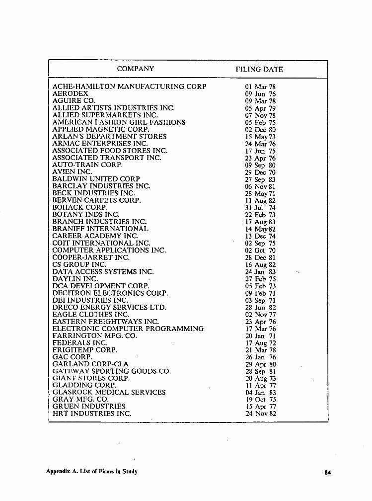
COMPANY FILING DATE
ACHE-HAMILTON MANUFACTURING CORP 01 Mar 78AERODEX 09 Jun 76AGUIRE CO. 09 Mar 78ALLIED ARTISTS INDUSTRIES INC. 05 Apr 79ALLIED SUPERMARKETS INC. 07 Nov 78AMERICAN FASHION GIRL FASHIONS 05 Feb 75APPLIED MAGNETIC CORP. 02 Dec 80ARLAN’S DEPARTMENT STORES 15 May 73ARMAC ENTERPRISES INC. 24 Mar 76ASSOCIATED FOOD STORES INC. 17 Jun 75ASSOCIATED TRANSPORT INC. 23 Apr 76AUTO-TRAIN CORP. 09 Sep 80AVIEN INC. 29 Dec 70BALDWIN UNITED CORP 27 Sep 83BARCLAY INDUSTRIES INC. 06 Nov 81BECK INDUSTRIES INC. 28 May71BERVEN CARPETS CORP. 11 Aug 82BOHACK CORP. 31 Jul 74BOTANY INDS INC. 22 Feb 73BRANCH INDUSTRIES INC. 17 Aug 83BRANIFF INTERNATIONAL 14 May 82CAREER ACADEMY INC. 13 Dec 74_COIT INTERNATIONAL INC. ‘ 02 Sep 75COMPUTER APPLICATIONS INC. 02 Oct 70COOPER-JARRET INC. 28 Dec 81CS GROUP INC. 16 Aug 82DATA ACCESS SYSTEMS INC. 24 Jan 83 ~~DAYLIN INC. — 27 Feb 75DCA DEVELOPMENT CORP. 05 Feb 73DECITRON ELECTRONICS CORP. 09 Feb 71DEI INDUSTRIES INC. 03 Sep 71DRECO ENERGY SERVICES LTD. 28 Jun 82EAGLE CLOTHES INC. 02 Nov 77EASTERN FREIGHTWAYS INC. 23 Apr 76ELECTRONIC COMPUTER PROGRAMMING 17 Mar 76FARRINGTON MFG.‘CO. 20 Jan 71FEDERALS INC. . 17 Aug 72FRIGITEMP CORP. 21 Mar 78GAC CORP. ° 26 Jan 76GARLAND CORP-CLA 29 Apr 80 .GATEWAY SPORTING GOODS CO. 28 Sep 81GIANT STORES CORP. 20 Aug 73 _GLADDING CORP. . II Apr 77GLASROCK MEDICAL SERVICES 04 Jan 83GRAY MFG. CO. 19 Oct 75GRUEN INDUSTRIES 15 Apr 77HRT INDUSTRIES INC. 24 Nov 82
Appendix A. List of Firms in Study 84
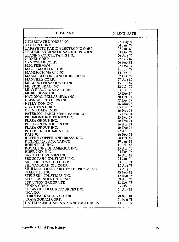
COMPANY FILING DATE
INTERSTATE STORES INC. 22 May 74KENTON CORP. 04 Jan 74LAFAYETTE RADIO ELECTRONIC CORP 07 Jan 80LEADER INTERNATIONAL INDUSTRIES 03 Dec 73LEASING CONSULTANTS INC. 20 Aug 70LIONEL CORP. 22 Feb 82LYNNWEAR CORP. 26 Feb 81M.H. FISHMAN 27 Dec 74MAGIC MARKER CORP. 21 Jun 79MAMMOTH MART INC. 14 Jun 74MANSFIELD TIRE AND RUBBER CO. 02 Oct 79MANVILLE CORP. 27 Aug 82MEGO INTERNATIONAL INC. 15 Jun 82MEISTER BRAU INC. I2 Jul 72MILO ELECTRONICS CORP. 03 Jul 70MOBIL HOME INC. 05 Dec 84NATIONAL BELLAS HESS INC. 30 Oct 74NEISNER BROTHERS INC. 02 Dec 77NELLY DON INC. 18 May78OLD TOWN CORP. 05 Jun 73OPEN ROADS INDS. 16 Nov 76PATERSON PARCHMENT PAPER CO. 23 Dec 74PIEDMONT INDUSTRIES INC. 23 Feb 79PLAZA GROUP INC. 10 Dec 74POLORON PRODUCTS INC. 14 Apr 81PLAZA GROUP INC. 10 Dec 74POTTER INSTRUMENT CO. 22 Apr 75 —-RAI INC. — 16 Feb 73REVERE COPPER AND BRASS INC. 28 Oct 82RICHMOND TANK CAR CO. 10 Jan 83ROBINTECH INC. II Jul 83ROYAL INNS OF AMERICA INC. 25 Apr 75RUPP. IND. INC. 05 Feb 76SAXON INDUSTRIES INC. I6 Apr 82SEQUOYAI·I INDUSTRIES INC. 24 Jan 74SHEFFIELD WATCH CORP. 03 Jun 71 ‘SIIENANDOAH OIL CORP. . 18 Aug 78SHULMAN TRANSPORT ENTERPRISES INC. 03 Aug 78STEELMET INC. ' 23 Feb 83STELBER INDUSTRIES INC. 12 Ma: 76 .STELLER INDUSTRIES INC. 09 Apr 75STRATTON GROUP LTD 18 Sep 73 .TENNA CORP . 05 Dec 79TEXAS GENERAL RESOURCES INC. 01 Apr 83TMA CO. 31 Jul 72TOBIN PACKAGING CO. INC. 28 Sep 81TRANSOGRAM CORP. 01 Mar 71UNITED MERCHANTS & MANUFACTURERS 13 Jul 77
Appendix A. List of Firms in Study 85
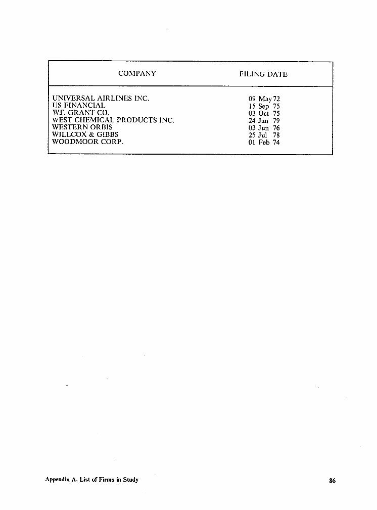
COMPANY FILING DATE
UNIVERSAL AIRLINES INC. 09 May 72US FINANCIAL I5 Sep 75WI. GRANT CO. 03 Oct 75WEST CI·IEMICAL PRODUCTS INC. 24 Jan 79WESTERN ORBIS 03 Jun 76WILLCOX & GIBBS 25 Jul 78WOODMOOR CORP. Ol Feb 74
Appendix A. List of Firms in StudyI
86
Appendix B. Logit Analyses with Overall
Average Imputation
Appcndix B. Logit Analyscs with Overall-Average lmputation 87

TABLE 4B
LOGIT ANALYSIS OF ACQUIRED VERSUS LIQUIDATED GROUPS
0 IF LIQUIDATED (N= 42)DEPENDENT VARIABLE : OUTCOME =
1 IF ACQUIRED(N=12)
-2 LOG LIKELIIIOOD FOR MODEL CONTAINING COUPERCEPT ONLY= 57.21
MODEL CHI-SQUARE= 12.19 WITH 11 D.F. (-2 LOG L.R.) P= 0.3494
VARIABLE BETA STD.ERROR CHI-SQUARE P
INTERCEPT -0.93189805 1.47226083 0.40 0.5268LAW -0.6623910l 1.10122380 0.36 0.5475BANK -2.58877558 2.24515564 1.33 0.2489TAX 0.00092791 0.00749712 - 0.02 0.9015LIQ 0.03161139 0.13528822 0.05 0.8152ROA 3.37456547 3.35975576 1.01 0.3152SIZE -0.00026704 0.00101622 0.07 0.7927COUP 22.0786289O 10.71053404 4.25 0.0393 **VAR 196.06851655 179.77011933 1.19 0.2754SKEW -0.05850846 0.10420944 0.32 0.5745FA 0.1 1508286 0.59896932 0.04 0.8476OWN -000124359 0.00070764 3.09 0.0789 *
* SIGNIFICANT AT 10% LEVEL** SIGNIFICANT AT 5% LEVEL**"' SIGNIFICANT AT 1% LEVEL
Appcndix B. Logit Analyscs with Ovcm1|·Avcragc Imputation 88
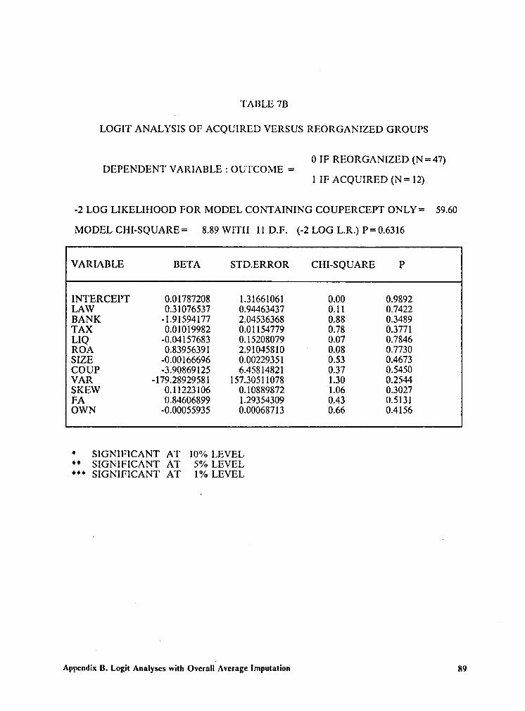
TABLE 7B
LOGIT ANALYSIS OF ACOUIRED VERSUS REORGANIZED GROUPS
0 IF REORGANIZED (N=47)DEPENDENT VARIABLE : OUTCOME =
1 IF ACQUIRED (N = 12)
-2 LOG LIKELIHOOD FOR MODEL CONTAINING COUPERCEPT ONLY= 59.60
MODEL CHI-SQUARE= 8.89 WITII 11 D.F. (-2 LOG L.R.) P=0.63l6
VARIABLE BETA STD.ERROR CHI·SQUARE P
INTERCEPT 0.01787208 1.31661061 0.00 0.9892LAW 0.31076537 0.94463437 0.11 0.7422BANK -1.91594177 2.04536368 0.88 0.3489TAX 0.01019982 0.01154779 0.78 0.3771LIQ -0.04157683 0.15208079 0.07 0.7846ROA 0.83956391 2.91045810 ‘ 0.08 0.7730SIZE -0.00166696 0.00229351 0.53 0.4673COUP -3.90869125 6.45814821 0.37 0.5450VAR - l79.28929581 157.30511078 1.30 0.2544SKEW 0.11223106 0.10889872 1.06 0.3027FA 0.84606899 1.29354309 0.43 0.5131OWN -0.0005593S 0.00068713 0.66 0.4156
* SIGNIFICANT AT 10% LEVEL** SIGNIFICANT AT 5% LEVEL*** SIGNIFICANT AT 1% LEVEL
Appcndix B. Logit Analyscs with Ovcmll-Avcrage Imputation 89
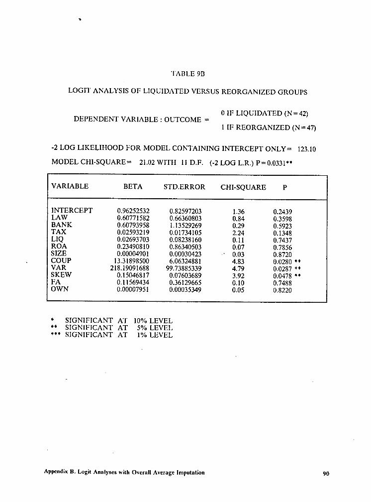
TABLE 9B
LOGIT ANALYSIS OF LIQUIDATED VERSUS REORGANIZED GROUPS
0 IF LIQUIDATED (N=42)DEPENDENT VARIABLE 1 OUTCOME =
1 IF REORGANIZED (N=47)
-2 LOG LIKELII·IOOD FOR MODEL CONTAINING INTERCEPT ONLY= 123.10
MODEL CHI-SQUARE= 21.02 WITH 11 D.F. (-2 LOG L.R.) P= 0.0331**
VARIABLE BETA STD.ERROR CHI-SQUARE P
INTERCEPT 0.96252532 0.82597203 1.36 0.2439LAW 0.60771582 0.66360803 0.84 0.3598BANK 0.60793958 1.13529269 0.29 0.5923TAX 0.02593219 0.01734105 2.24 0.1348LIQ 0.02693703 0.08238160 0.11 0.7437ROA 0.23490810 0.86340503 0.07 0.7856SIZE 0.00004901 0.00030423 —‘ 0.03 0.8720
. COUP 13.3189850O 6.06324881 4.83 0.0280 **VAR 218.19091688 99.73885339 4.79 0.0287 **SKEW 0.15046817 0.07603689 3.92 0.0478 "‘*FA 0.11569434 0.36129665 0.10 0.7488OWN 0.00007951 0.00035349 0.05 0.8220
* SIGNIFICANT AT 10% LEVEL** SIGNIFICANT AT 5% LEVEL**"' SIGNIFICANT AT 1% LEVEL
Appcndix B. Logit Analyscs w·ith OvcraIlKAvcragc lmputation 90

TABLE 12B
LOGIT ANALYSIS OF LIQUIDATED VERSUS CONTINUED GROUPS
0 IF LIQUIDATED (N = 42)DEPENDENT VARIABLE 2 OUTCOME =
1 IF ACQUIRED (N= 59)
-2 LOG LIKELIHOOD FOR MODEL CONTAINING INTERCEPT ONLY= 137.14
MODEL CHI-SQUARE= 19.03 WITH 11 D.F. (-2 LOG L.R.) P=0.0605 *
VARIABLE BETA STD.ERROR CHI-SQUARE P
INTERCEPT -0.74256765 0.80130424 0.86 0.3541LAW -0.57269883 0.61826073 0.86 0.3543BANK 0.18388143 1.09285360 0.03 0.8664TAX -0.00480694 0.00442431 1.18 0.2773LIQ ~0.03064534 0.07971496 0.15 0.7007ROA 0.16813166 0.77051817 0.05 0.8273SIZE ·0.00010077 0.00027512 0.13 0.7142COUP 15.9542131I 6.01584586 7.03 0.0080 ***VAR 169.63166212 8989486777 3.56 0.0592 *SKEW -0.11760456 0.06562464 3.21 0.0731 *FA -0.07971167 0.35670919 0.05 0.8232OWN -0.00017704 0.00034561 0.26 0.6085
* SIGNIFICANT AT 10% LEVEL** SIGNIFICANT AT 5% LEVEL*** SIGNIFICANT AT 1% LEVEL
Appcndix B. Logit Analyscs with Ovcra11.Avcragc Imputation 91