why were latin america’s tariffs so much higher than … were latin america’s tariffs so much...

WHY WERE LATIN AMERICA’S TARIFFS SOMUCH HIGHER THAN ASIA’S BEFORE 1950?*

MICHAEL A. CLEMENSCenter for Global Development a

JEFFREY G. WILLIAMSONHarvard University and the University of Wisconsin b

ABSTRACT

Latin America had the highest tariffs in the world before 1914; Asia hadthe lowest. Heavily protected Latin America also boasted some of the mostexplosive belle epoque growth, while open Asia registered some of the least.What brought the two regions to the opposite ends of the tariff policy spectrum?We find that limits to Asian tariff policy autonomy may have lowered tariffssubstantially there, but by themselves they cannot explain why Asian tariffswere so much lower than the Latin American tariffs before 1914; that naturalbarriers, domestic political economy and strategic tariff policy seems to havecontributed much to the difference and that the origins of Asian post-WorldWar 2 import-substitution policies seem to lie in the interwar years when Asiantariff levels caught up with those of Latin America.

Keywords: tariffs, Latin America, Asia, growth, history

JEL Code: F13, N70, O24

RESUMEN

America Latina tuvo los aranceles mas altos del mundo antes de 1914;Asia tuvo los mas bajos. Fuertemente protegida, America Latina tambien

* Received 12 April 2011. Accepted 19 July 2011.a 1800 Massachusetts Avenue NW, 3rd floor, Washington, DC 20036, USA. [email protected] 350 South Hamilton Street, Unit 1002, Madison, WI 53703, USA. [email protected].

Revista de Historia Economica, Journal of lberian and Latin American Economic HistoryVol. 30, No. 1: 11-44. doi:10.1017/S021261091100019X & Instituto Figuerola, Universidad Carlos III de Madrid, 2011.

11

ofrecio uno de los crecimientos mas explosivos de la belle epoque mientrasAsia mostraba uno de los menores. +Fue el diferente espectro de la polıticaarancelaria lo que llevo a estas dos regiones a destinos tan opuestos? Nosotrosencontramos: que los lımites a la autonomıa de la polıtica arancelaria en Asiahabrıan contribuido considerablemente a reducir los aranceles, pero no pue-den explicar por sı mismos por que los aranceles fueron mucho mas bajos queen America Latina antes de 1914; las barreras naturales, la economıa polıticanacional y las polıticas arancelarias estrategicas parecen haber contribuidomucho a la diferencia en el comportamiento del crecimiento de estas dos zonasy los orıgenes de la polıtica de sustitucion de importaciones asiatica posterior ala II Guerra Mundial parecen extenderse al periodo de entreguerras cuando losniveles arancelarios asiaticos convergieron con los de America Latina.

Palabras clave: aranceles, America Latina, Asia, crecimiento, historia

1. INTRODUCTION

While many have compared Latin American and Asian trade policy since1950, few have extended the comparison to the preceding century. The bestevidence from the long 19th century through World War (WW) 2 revealstremendous contrasts between the two regions. These demand explanation.

Latin America had the highest tariffs in the world before 1914; Asia hadthe lowest. The Latin American belle epoque also boasted some of the highestgrowth rates, while Asia registered some of the lowest. What brought the tworegions to the opposite ends of the tariff policy spectrum? Was it simply thatLatin America had policy autonomy, while most of colonial Asia did not, orwas the political economy of tariffs more complex? Why did Asian tariffscatch up with those high Latin American tariffs in the 1920s and 1930s? Dohistorical patterns of growth and tariff policy in the two regions accord withrecent conventional wisdom that free trade fosters growth?

This paper uses the historical record of tariff policy to begin anexploration of all of these questions. We use average ad valorem-equivalenttariff rates and describe their correlates with tariff autonomy and otherpolitical economy forces in the two regions. Average tariff rates cannot, ofcourse, settle questions about «protection» more generally, which includespolicies other than tariffs, and they lack fine-grained information aboutrelative protection of different industries. Since overall tariffs differed vastlybetween the two regions, they are certainly a good place to begin.

We first describe our tariff database. We use these data to explore the partialcorrelations between import duty levels and the conditions under which theywere set — including colonial rule, «unequal treaties», world market condi-tions, geography and the local political economy environments. We find thatwhile limits to Asian tariff policy autonomy certainly lowered tariffs there

MICHAEL A. CLEMENS/JEFFREY G. WILLIAMSON

12 Revista de Historia Economica, Journal of lberian and Latin American Economic History

substantially, they cannot by themselves explain why Asian tariffs were somuch lower than the Latin American tariffs before 1914; that natural barriers,domestic political economy and strategic tariff policy seem to have contributedmuch to the difference and that the origins of Asian post-WW2 import-sub-stitution policies seem to lie in the interwar years when Asian tariffs caught upwith those of Latin America. At the end of the paper, we pose a researchagenda: Does tariff policy explain most of the differences in industrialisationexperience within and between the two regions, or did other factors — liketerms of trade trends, the evolution of wage, fuel, and intermediate costs andproductivity catch up with the leaders — matter much more?

2. THE TARIFF DATA

A well-developed international literature makes it clear that trade sharesare very poor measures of openness, since they are endogenous and can bedriven by demand and supply factors within countries that are completelyindependent of trade policy1. Among the explicit policy measures of opennessavailable, the average tariff rate is by far the most homogeneous protectionmeasure and the easiest to collect across countries and over time. We are, ofcourse, aware that countries can have the same average tariff levels, but verydifferent tariff structures2. Nevertheless, high average tariffs typically meanteven higher tariffs on manufactures in primary-product exporting countries3.We are also aware that by the late 1930s every country had learnt how to usenon-tariff barriers (NTBs), especially the manipulation of the real exchangerate to favour import-competing industries. However, NTBs were not usedvery frequently before the early 1930s, and nearly every country was on a fixedexchange standard before WW1 and again in the 1920s. In short, tariffs werethe main instrument of trade policy before the 1930s. In any case, high tariffswere also positively correlated with the use of NTBs. Thus, it seems to us that

1 For example, see Anderson and Neary (1994), Sachs and Warner (1995) and Anderson (1998).Indeed, it appears that totally 67 per cent of the late 20th century Organisation for EconomicCooperation and Development trade boom can be explained by unusually fast income growth, andnot by the decline in trade barriers (Baier and Bergstrand 2001). To cite another example, 50 to 65per cent of the European overseas trade boom in the three centuries following 1492 were driven byincome growth, rather than by any decline in trade barriers (O’Rourke and Williamson 2002,p. 439). As a final example, 57 per cent of the world trade boom from 1870 to 1913 was explained bythe income growth (Estevadeordal et al. 2003, Table III).

2 See, for example, Lehmann and O’Rourke (2011) on 19th century Europe, and Nunn andTrefler (2010) on the 20th century world economy.

3 See, for example, Bairoch (1993) and Williamson (2011a, Ch. 13). Antonio Tena (personalcorrespondence) has estimated ad valorem tariffs on British manufacturing exports for four LatinAmerican republics in 1914 (Argentina, Brazil, Chile and Mexico): while the tariff for all importsaveraged 21.5 per cent, the average tariff on British manufactures averaged 45 per cent, more thantwice as high. Similarly, for the European periphery (Greece, Italy, Portugal, Russia, Spain): whilethe average tariff on all imports in 1914 was 18.4 per cent, the tariff on British manufactures was46.2 per cent, almost three times higher.

LATIN AMERICA’S TARIFFS VS. ASIA’S PRE-1950

Revista de Historia Economica, Journal of lberian and Latin American Economic History 13

as an overall measure of protection, average tariffs are the place to start anyempirical analysis of the political economy of protection, even if they are notthe place to finish it. In addition, while high tariffs may not necessarily be theresult of explicit pro-industrialisation goals, they are protectionist regardlessof their motivation.

This paper uses the computed average tariff rate to explore differencesbetween Asian and Latin American policy experience from shortly after the mid-19th century to WW2. Our country observations from these two regions are partof a larger world sample of thirty-five, extending up to 1950: the United States;three members of the European industrial core (France, Germany and the UnitedKingdom); three English-speaking European offshoots (Australia, Canada andNew Zealand); ten from the European periphery (Austria–Hungary, Denmark,Greece, Italy, Norway, Portugal, Russia, Serbia, Spain and Sweden); ten fromAsia and the Middle East (Burma, Ceylon, China, Egypt, India, Indonesia, Japan,the Philippines, Siam (Thailand) and the Ottoman Empire (republican Turkey));and eight from Latin America (Argentina, Brazil, Chile, Cuba, Colombia, Mexico,Peru and Uruguay). Standard tariff histories focus mainly on seven — Denmark,France, Germany, Italy, Sweden, the United Kingdom and the United States.While the tariff data used here have already been exploited to help redress thisbig world research imbalance (O’Rourke and Williamson 2002; Clemens andWilliamson 2004; Coatsworth and Williamson 2004a, 2004b; Williamson 2006b),this paper does much more by focusing in depth on the ten Asian and eight LatinAmerican countries in our sample, which represent the poor periphery, and byexploring the crucial interwar experience as well.

Average tariff rates are calculated as the total revenue from import dutiesdivided by the value of total imports in the same year. In some cases, thesources used do not distinguish between import and export duties, and reportonly total customs duties. However, total customs duties (instead of importduties) are used in the calculation of average tariff rates only for countrieswhere the value of export duties have historically been an insignificant shareof total customs duties. Sometimes, the value of import duties collected isreported for fiscal years, while import data generally refer to calendar years.While making a consistent effort to compare calendar year duties withcalendar year import values, in cases where calendar year duties figures areunavailable, fiscal year duties are divided by calendar year imports to calculateaverage tariff. In these instances, fiscal year import duties are assumed tobelong to the calendar year in which most of the fiscal year falls4.

The remainder of this paper defines Latin America as the eight-countrysample consisting of Argentina, Brazil, Chile, Colombia, Cuba, Mexico, Peruand Uruguay. Asia is defined as the ten-country sample consisting of Burma,China, Ceylon, Egypt, India, Indonesia, Japan, the Philippines, Siam and

4 A complete appendix description of the sources and methods surrounding the tariff databasecan be found in Blattman et al. (2002) and Clemens and Williamson (2004).



Turkey, while East Asia is defined by the sub-sample of China, Indonesia,Japan, the Philippines and Siam.

3. EXPLORING TARIFF AUTONOMY

Our analysis requires formalisation of the concept of tariff autonomy, thefreedom to set tariff levels independent of another state’s military and poli-tical power. Table 1 lists the years in which we judge each country to havehad tariff autonomy. Burma, Ceylon and India were subject to Britishimperial tariff collection policies, as Cuba was to the Spanish through 1899,Indonesia (Netherlands Indies) was to the Dutch and the Philippines was toboth the Spanish up to 1898 and the United States thereafter. The BritishForeign Office in China largely eliminated the tariff restrictions imposed bythe treaties of Nanking and Tientsin in 1929. Norway did not have an inde-pendent tariff policy under the Swedish crown through 1905. Gradual weak-ening of Ottoman control in Serbia is construed to imply tariff autonomyfollowing the 1878 Treaty of Berlin. Egypt is taken to hold tariff autonomyunder non-interventionist Ottoman rule during the years prior to the Britishinvasion of 1882, but not thereafter. Thailand is taken to recover autonomyfrom the grasp of the unequal treaties in 1891, following Ingram (1971,p. 138), and Japan in 1900, following Lockwood (1968, p. 539). We takeTurkey to have lost tariff autonomy in the brief years between its defeat inWW1 and Mustafa Kemal’s establishment of the Turkish Republic thereafter.

With these definitions of tariff autonomy in mind, we turn next to colonialtariff policy, followed by tariff policy under gunboat diplomacy.

3.1. Did Asian Colonies Simply Mimic their Masters?

This is a good place to explore the tariff autonomy issue within thecolonies. There are five colonies in our sample, all in Asia: Burma, Ceylon,India, Indonesia and the Philippines, although foreign influence was strongenough (including occupation) to make Egypt behave like a colony after 1881(see, e.g. Owen 1993, p. 122). To what extent did these six simply mimic theircolonial masters?

Figure 1 reveals a clear correlation in timing and magnitudes of change intariff rates between the United Kingdom and her four colonies in the sample(Burma, Ceylon, Egypt and India). Figure 2 shows the same for the Philippines,first for Spain and then for the United States (becoming the imperialist masterin 1899). Table 2 reports the master colony tariff rate correlations for these fourand for the Philippines5. Colonial tariff policy did indeed mimic that of the

5 The Netherlands is not part of our sample, and thus we cannot explore the same correlationsbetween it and Indonesia.



TABLE 1TARIFF AUTONOMY 1870-1938

Over the years spanning from 1870 to 1938, the periods during which countries aredeemed to have autonomy over setting tariff rates were (see text):

Argentina All

Australia All

Austria/Austria–Hungary All

Brazil All

Burma None

Canada All

Ceylon None

Chile All

China 1929 and after

Colombia All

Cuba 1899 and after

Denmark All

Egypt Before 1882

France All

Germany All except 1919-1925

Greece All

India None

Indonesia None

Italy All

Japan 1900 and after

Mexico All

New Zealand All

Norway 1906 and after

Peru All

Philippines None

Portugal All

Russia/USSR All

Serbia/Yugoslavia 1878 and after

Spain All

Sweden All

Thailand 1891 and after

Turkey All except 1919-1923

United Kingdom All

United States All

Uruguay All



FIGURE 1BRITISH TARIFFS VS. TARIFFS IN THE EMPIRE

0

5

10

15

20

25

30

35

40

45

50

1860

Imp

ort

du

ties

/ Im

po

rts

United KingdomCeylonIndiaBurmaEgypt

1870

1880

1890

1900

1910

1920

1930

1940

1950

1960

FIGURE 2FILIPINO TARIFFS VS. SPANISH AND AMERICAN TARIFFS

0

10

20

30

40

50

60

Imp

ort

du

ties

/ Im

po

rts

United StatesSpainPhilippines

1860

1960

1870

1880

1890

1900

1910

1930

1920

1940

1950



masters: although Spain failed to imprint its tariff rates on the Philippinesbefore 1899 (Figure 2), the United States did afterwards, and Britain did soacross all four of its Asian colonies in our sample (Figure 1). Furthermore, thet-statistics are very large, and the slope coefficients are similar across mastersand colonies, ranging approximately between 0.5 and 0.9.

However, note the variance across these four at any point in time (Figure 1),and note the country-specific variance in the intercepts reported for the five inTable 2. The Philippine tariff rates were on average approximately two pointsbelow the United States after 1898; and compared with Britain, India’s tariffrates were approximately the same, Burma and Ceylon were four or five pointshigher, and Egypt’s were ten points higher. Clearly, local conditions matteredeven in colonies. Thus, we retain the full Asian sample in all that follows,although we will control for the tariff policy of the masters.

There are three surprises that emerge from this section. First, tariff policycorrelates with local conditions even in the colonies. For example, in the1930s tariff rates ranged between 9.9 per cent in the Philippines and 28.7 per cent

TABLE 2CORRELATION BETWEEN TARIFFS IN COLONIES AND THEIR COLONIAL

MASTERS

Country’s tariff asdependent variance Egypt Burma Ceylon India Philippines Philippines

Time period1865-1945

1865-1945

1865-1945

1865-1945 1865-1898 1899-1945

UK tariffs 0.607 0.672 0.493 0.893

6.65 8.62 17.5 16.5

0.587 0.685 0.886 0.874

Spain tariffs 20.0807

20.456

20.0791

USA tariffs 0.870

10.2

0.839

Constant 10.0 4.84 4.32 0.198 11.4 22.16

7.51 4.25 10.5 0.249 3.49 21.47

N 86 86 86 86 35 46

R2 0.345 0.469 0.785 0.763 0.00630 0.704

Note: Ordinary least squares regressions. t-statistics are in italics and standardized coefficients are inbold below each coefficient.



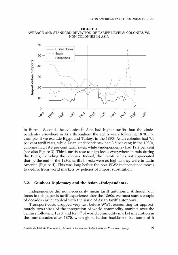
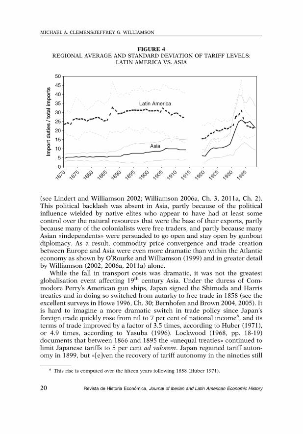
in Burma. Second, the colonies in Asia had higher tariffs than the «inde-pendents» elsewhere in Asia throughout the eighty years following 1870. Forexample, if we exclude Egypt and Turkey, in the 1890s Asian colonies had 7.1per cent tariff rates, while Asian «independents» had 3.8 per cent; in the 1930s,colonies had 19.3 per cent tariff rates, while «independents» had 17.3 per cent(see also Figure 3). Third, tariffs rose to high levels everywhere in Asia duringthe 1930s, including the colonies. Indeed, the literature has not appreciatedthat by the end of the 1930s tariffs in Asia were as high as they were in LatinAmerica (Figure 4). This was long before the post-WW2 independence movesto de-link from world markets by policies of import substitution.

3.2. Gunboat Diplomacy and the Asian «Independents»

Independence did not necessarily mean tariff autonomy. Although ourfocus in this paper is tariff experience after the 1860s, we must start a coupleof decades earlier to deal with the issue of Asian tariff autonomy.

Transport costs dropped very fast before WW1, accounting for approxi-mately two-thirds of the integration of world commodity markets over thecentury following 1820, and for all of world commodity market integration inthe four decades after 1870, when globalisation backlash offset some of it

FIGURE 3AVERAGE AND STANDARD DEVIATION OF TARIFF LEVELS: COLONIES VS.

NON-COLONIES IN ASIA

0

10

20

30

40

50

60

Imp

ort

du

ties

/ Im

po

rts

United StatesSpainPhilippines

1860

1960

1870

1880

1890

1900

1910

1930

1920

1940

1950



(see Lindert and Williamson 2002; Williamson 2006a, Ch. 3, 2011a, Ch. 2).This political backlash was absent in Asia, partly because of the politicalinfluence wielded by native elites who appear to have had at least somecontrol over the natural resources that were the base of their exports, partlybecause many of the colonialists were free traders, and partly because manyAsian «independents» were persuaded to go open and stay open by gunboatdiplomacy. As a result, commodity price convergence and trade creationbetween Europe and Asia were even more dramatic than within the Atlanticeconomy as shown by O’Rourke and Williamson (1999) and in greater detailby Williamson (2002, 2006a, 2011a) alone.

While the fall in transport costs was dramatic, it was not the greatestglobalisation event affecting 19th century Asia. Under the duress of Com-modore Perry’s American gun ships, Japan signed the Shimoda and Harristreaties and in doing so switched from autarky to free trade in 1858 (see theexcellent surveys in Howe 1996, Ch. 30; Bernhofen and Brown 2004, 2005). Itis hard to imagine a more dramatic switch in trade policy since Japan’sforeign trade quickly rose from nil to 7 per cent of national income6, and itsterms of trade improved by a factor of 3.5 times, according to Huber (1971),or 4.9 times, according to Yasuba (1996). Lockwood (1968, pp. 18-19)documents that between 1866 and 1895 the «unequal treaties» continued tolimit Japanese tariffs to 5 per cent ad valorem. Japan regained tariff auton-omy in 1899, but «[e]ven the recovery of tariff autonomy in the nineties still

FIGURE 4REGIONAL AVERAGE AND STANDARD DEVIATION OF TARIFF LEVELS:

LATIN AMERICA VS. ASIA

0

5

10

15

20

25

30

35

40

45

50

1930

Imp

ort

du

ties

/ to

tal i

mp

ort

s

Latin America

Asia

1870

1875

1880

1885

1890

1895

1900

1905

1910

1915

1920

1925

1935

6 This rise is computed over the fifteen years following 1858 (Huber 1971).



left treaty restrictions on the duties applying to many items. Rates weregenerally no higher than 10-15 per cent until the general tariff revision of1911» (Lockwood 1968, p. 539).

Other Asian nations followed the same liberal path, most forced to do soby colonial dominance or gunboat diplomacy. Thus, and even before theJapanese humiliation, China signed a treaty with Britain in 1842 that openedher ports to trade. The treaties of Nanking (1843), Tientsin (1858) and otherslike them, limited the Chinese ad valorem tariff rate on imports fromessentially all of Europe to 5 per cent. In fact, the treaties (and their revisionsin 1870, 1902 and 1922) did not set ad valorem rates but rather nominalspecific duties that, although initially equivalent to a 5 per cent ad valorem tariff,rapidly declined in effective value as prices rose (Remer 1926, pp. 171-181).Siam avoided China’s humiliation by going open on its own and adopting a 3per cent tariff limit in 1855. Between 1865 and 1890, treaties with all the majorpowers kept import duties below 3 per cent in Siam. Only after 1890 did Siambegin to revise the earlier treaties and increase tariff revenue by raising its tariffrates (Ingram 1971, pp. 34-35, 138). Korea emerged from being the autarkicHermit Kingdom about the same time, undergoing market integration withJapan long before colonial status became formalised in 1910 (Brandt 1993;Kang and Cha 1996). India went the way of British free trade in 1846, andIndonesia followed Dutch liberalism. Thus, and in sharp contrast with Europe(and its hostile grain invasion response) and Latin America (and its even morehostile manufactures invasion response), sharply declining transport costs werenot offset in Asia by a rise in tariffs.

4. SOME LATIN AMERICAN BELLE EPOQUE SURPRISES

Coatsworth and one of the present authors (Coatsworth and Williamson2004a, 2004b) recently uncovered some facts that had not been well appre-ciated: Tariffs in Latin America were far higher than anywhere else in theworld during the decades before WW1. This was long before the GreatDepression, after which the region retreated into what became known asImport Substituting Industrialisation (ISI). Indeed, tariffs were even rising inthe decades before 1914, a period that has been identified by O’Rourke andWilliamson (1999) the first globalisation boom for the world economy. Thisfact is surprising, and for three reasons: first, it comes as a surprise given thatthis region has been said to have exploited globalisation forces better thanmost of the poor periphery during the pre-1914 belle epoque (Bulmer-Thomas1994, Ch. 4); second, it comes as a surprise since standard economic historiessay so little about it7; and third, it comes as a surprise since most have alwaysbeen taught to view the Great Depression as the critical turning point when

7 See Gomez Galvarriato and Williamson (2009) for one recent exception to this generalization.



the region is said to have turned towards protection and de-linked from theworld economy for the first time (for three often cited examples, see Diaz-Alejandro 1984; Corbo 1992; Taylor 1998).

These Latin American surprises can be seen in Figure 4, but they can beappreciated even better by comparisons with the rest of the world. As wenoted above, conventional wisdom is that Latin American reluctance to goopen in the mid-late 20th century was the product of the Great Depressionand the anti-global import-substitution strategies that arose to deal with it.Yet, late 19th century Latin America already had by far the highest tariffs inthe world. For example, in 1885 the poor but independent parts of LatinAmerica (Brazil, Colombia, Mexico and Peru) had tariffs almost five timeshigher than those in the poor and dependent parts of Asia (Burma, Ceylon,China, Egypt, India, Indonesia and the Philippines). Perhaps more to thepoint, in the decades before 1914 tariffs in Latin America were, on average,five times higher than those in the European industrial core of Britain,France and Germany!

At the crescendo of the belle epoque, Latin American tariffs were at theirpeak, and still far above tariffs in the rest of the world. For example, in 1905tariffs in Uruguay (the most protectionist, land-abundant and labour-scarcecountry) were approximately two and a half times those in Canada (the leastprotectionist, land-abundant and labour-scarce country). In the same year,tariffs in Brazil and Colombia (the most protectionist Latin Americancountries) were almost ten times those in China and India (the least pro-tectionist in Asia). Furthermore, the rise in Latin American tariffs from thelate 1860s to the turn of the century was much steeper than was true ofEurope, including France and Germany about which so much tariff historyhas been written by scholars like Gerschenkron (1943), Kindleberger (1951),Bairoch (1989) and, more recently, O’Rourke (2000). For example, the rise inthe average tariff rate between the 1870s and the 1890s was 5.7 percentagepoints in France, up from 4.4 per cent to still only 10.1 per cent, and5.3 percentage points in Germany, up from 3.8 to still only 9.1 per cent. Thisheavily researched continental move to protection is pretty modest whencompared with the rise over the same period in the four poor Latin Americancountries (up from 6.9 percentage points to 34 per cent), and this for a regionthat has been said to have exploited the pre-1914 globalisation boom so wellby allowing exports to be an engine of growth.

5. CLOSED JAGUAR, OPEN DRAGON?

Figure 4 reveals the stark difference between Latin American and Asiantariff policy that persisted over the century between the 1860s and the eve ofthe WW2. Black lines show regional means, while grey bands indicate one(regional) standard deviation above and below that mean.



Note the collapse in tariff rates across WW1, a worldwide phenomenon dueto the tendency for wartime inflation to erode the ad valorem equivalent ofwhat were largely specific duties, not principally the result of tariff policychanges. The inflation-induced wartime fall was partially recovered in the post-war deflations of the late 1910s and early 1920s. Note also that the tariff ratesurged in the early 1930s, spiking in 1933, again repeated across the globe, asworld price levels collapsed, raising the ad valorem equivalent of those specificduties, not the result of tariff policy changes. However, both Latin Americanand Asian tariff rates continued to rise after the world recovery and price rise:indeed, they rose more in Asia, reaching parity with and even exceeding pro-tectionist Latin America 1934-1939. Of course, tariff rates were raised partly inresponse to America’s Hawley–Smoot Act; however, the main point is that tariffrates rose to high levels in Asia and Latin America even after prices began toinflate during the recovery from the Great Depression.

The impact of inflation and deflation on ad valorem tariff rate equivalentswas huge in Asia and Latin America since the poor periphery relied soheavily on specific duties (e.g. pesos per pound, francs per bale, dollars peryard). Why were (and are) specific duties so common in poor parts of theworld? There are two possible explanations. First, honest and literate cus-toms inspectors are scarce in poor countries, but honest and literate customsinspectors are needed to implement an ad valorem tariff where importvaluation is so crucial. So, legislators imposed specific duties to minimise the«theft» of state tariff revenues by dishonest and illiterate customs agents.Second, specific duties are more effective macro-stabilisation devices inpoor countries that rely so heavily on customs duties as a source of totalgovernment revenue. During booms, prices rise, lowering the effectivetariff rates from specific duties, thus tending to mute the boom in tariffrevenues generated by the boom in import demand. During slumps, pricesfall, raising effective tariff rates, thus tending to offset the fall in tariff rev-enues generated by the slump in import demand. These macro-stabilisationforces would be all the more valuable in pre-WW2 Latin America andAsia when both regions were susceptible to great price volatility in theircommodity export markets8.

Table 3 summarises the variance in tariff rates before 1914. The averageLatin American country had four times the tariff level of the average Asiancountry. Table 4 gives average tariffs for each country during three differenttime periods (1870-1899, 1900-1913 and 1919-1938). Setting aside for amoment the relatively high tariffs of the Philippines, every Asian country hadlower tariffs than every Latin country before 1914. That was not true afterWW1, however, when three Asian countries nudged their tariff rates up in to

8 The literature on commodity price volatility and its impact is very large. See, for example,Blattman et al. (2002, 2007), Poelhekke and van der Ploeg (2007), Jacks et al. (2011), Williamson(2011a, Ch. 10) and van der Ploeg (2011).



Latin American ranges (Burma, Egypt, Turkey). Moreover, to repeat, by thelate 1930s Asia on average had higher tariffs than Latin America.

Figure 5 presents cross-sectional unweighted average GDP per capita, in1990 US$, for the two regions. Despite variation within the sample and inter-war troubles, the big morals of Figure 5 are that Latin America started from afar richer resource base and thus a much higher per capita income; her belleepoque growth experience left Asia far behind, but the GDP per capita gapbetween Latin America and Asia stopped widening in the interwar decades.

Were high tariffs associated with fast growth? Latin America had enormoustariffs and an impressive growth performance, while Asia had low tariffs andslow growth. However, Figure 6 shows that within these two regions, hightariffs are correlated with slow growth. So it looks like third forces mightaccount for the regional growth differences. Future research might do well toexplore this issue at greater length by looking at industrialisation and thirdfactors, a point we will raise again at the end of this paper.

6. WHY WERE LATIN AMERICAN TARIFFS SO MUCH HIGHERTHAN ASIAN TARIFFS BEFORE WW1?

Table 5 seeks to determine some of the correlates of the vastly differenttariff levels between Latin America and Asia before 1914. It certainly does

TABLE 3REGIONAL SUMMARY OF TARIFF LEVELS, 1870-1913

Mean Std. dev. Min Max Observations

Latin America1

Overall 27.0 8.76 9.7 58.2 N 5 341

Between 6.84 Groups 5 8

Within 6.04 T 5 43

Asia2

Overall 7.04 4.29 1.78 23.5 N 5 440


Within 2.79 T 5 44

East Asia3

Overall 6.70 4.80 1.78 23.5 N 5 220


Within 3.05 T 5 44

1Argentina, Brazil, Chile, Colombia, Cuba, Mexico, Peru and Uruguay.2Burma, China, Ceylon, Egypt, India, Indonesia, Japan, Philippines, Siam and Turkey.3China, Indonesia, Japan, Philippines and Siam.



not estimate a well-specified reduced-form model of the determinants oftariffs, so the coefficients estimated there cannot be given a simple causalinterpretation. Large coefficients can represent the influence of reversecausation or the influence of omitted factors; small coefficients can reflectoverlapping and countervailing effects. Nevertheless, it needs to be stressedthat corroboration of theory advances the scientific enterprise even whenstrict hypothesis testing is difficult, as it certainly is in this setting.

Table 5 explores cross-sectional differences in country tariffs for all thirty-five countries in the world sample, not just those in Asia and Latin America.These regressions use a panel between effects estimator, since the relation-ships we seek are cross-sectional — Latin America vs. Asia. The first threecolumns address the fact that coverage of the inflation regressor in ourdatabase is limited to thirty of the thirty-five countries. The first column thusanalyses the full sample; the second column includes the same regressors,but restricts the sample to data points for which inflation is not missing; and

TABLE 4AVERAGE TARIFF LEVELS BY PERIOD 1870-1938

1870-1899 1900-1913 1919-1938

Argentina 26.1 23.4 18.0

Brazil 34.5 40.0 23.4

Chile 19.4 18.3 22.1

Colombia 33.5 47.4 29.3

Cuba 22.5 25.6 26.2

Mexico 16.6 21.9 21.2

Peru 32.4 23.2 16.3

Uruguay 29.7 33.3 19.6

China 3.2 3.3 11.3

Indonesia 4.9 5.2 10.0

Japan 6.2 7.7 5.9

Philippines 10.3 21.2 8.1

Siam 3.6 7.4 15.1

Burma 4.0 11.3 22.5

Ceylon 6.2 7.3 13.3

Egypt 11.0 14.2 26.3

India 3.4 4.7 17.3

Turkey 7.4 9.5 30.7

Note: Tariffs are expressed as total import duties collected divided by total imports (%).



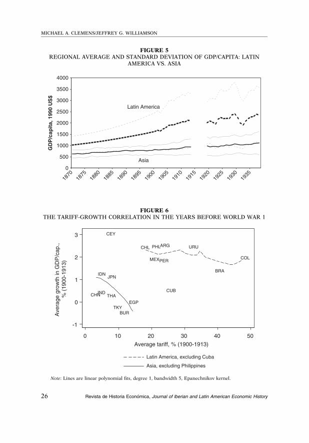
FIGURE 5REGIONAL AVERAGE AND STANDARD DEVIATION OF GDP/CAPITA: LATIN

AMERICA VS. ASIA

0

500

1000

1500

2000

2500

3000

3500

4000

1935

GD

P/c

apit

a, 1

990

US

$

Latin America

Asia

1870

1875

1880

1885

1890

1895

1900

1905

1910

1915

1920

1925

1930

FIGURE 6THE TARIFF-GROWTH CORRELATION IN THE YEARS BEFORE WORLD WAR 1

ARG

BRA

BUR

CEY

CHL

CHN

COL

CUB

EGP

IDN

IND

JPN

MEXPER

PHL

THA

TKY

URU

-1

0

1

2

3

Ave

rage

gro

wth

in G

DP

/cap

., %

(19

00-1

913)

0 10 20 30 40 50

Average tariff, % (1900-1913)

Latin America, excluding Cuba

Asia, excluding Philippines

Note: Lines are linear polynomial fits, degree 1, bandwidth 5, Epanechnikov kernel.



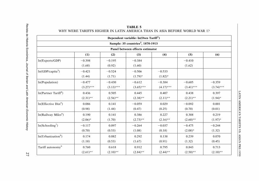
TABLE 5WHY WERE TARIFFS HIGHER IN LATIN AMERICA THAN IN ASIA BEFORE WORLD WAR 1?

Dependent variable: ln(Own Tariff1)

Sample: 35 countries2, 1870-1913

Panel between effects estimator

(1) (2) (3) (4) (5) (6)

ln(Exports/GDP) 20.398 20.195 20.384 20.410

(1.68) (0.92) (1.60) (1.62)

ln(GDP/capita3) 20.421 20.524 20.506 20.533

(1.44) (1.71) (1.79)* (1.82)*

ln(Population) 20.477 20.430 20.612 20.384 20.605 20.359

(3.27)*** (3.13)*** (3.65)*** (4.17)*** (3.41)*** (3.74)***

ln(Partner Tariff4) 0.436 0.505 0.445 0.407 0.438 0.397

(2.31)** (2.56)** (2.38)** (2.11)** (2.21)** (1.94)*

ln(Effective Dist5) 0.086 0.141 20.059 0.029 20.092 0.001

(0.98) (1.44) (0.47) (0.25) (0.70) (0.01)

ln(Railway Miles6) 0.190 0.141 0.386 0.227 0.388 0.219

(2.06)* (1.70) (2.73)** (2.16)** (2.60)** (1.97)*

ln(Schooling7) 20.117 0.097 20.264 20.037 20.475 20.244

(0.70) (0.53) (1.08) (0.18) (2.08)* (1.32)

ln(Urbanization8) 0.174 0.082 0.292 0.138 0.239 0.070

(1.18) (0.53) (1.67) (0.91) (1.32) (0.45)

Tariff autonomy9 0.760 0.618 0.912 0.795 0.843 0.713

(2.61)** (2.10)** (2.84)** (2.44)** (2.50)** (2.10)**

LA

TIN

AM

ER

ICA

’ST

AR

IFF

SV

S.

AS

IA’S

PR

E-1950

Revis

tade

His

toria

Econom

ica,

Journ

alof

lberia

nand

Latin

Am

eric

an

Econom

icH

isto

ry27

TABLE 5 (Cont.)

Dependent variable: ln(Own Tariff1)



(1) (2) (3) (4) (5) (6)

Inflation 20.030 0.034 20.037 0.030

(0.39) (0.50) (0.47) (0.43)

Inflation squared 0.003 0.002 0.003 0.002

(2.10)* (1.43) (2.07)* (1.39)

Constant 5.435 4.989 7.030 5.870 5.261 3.918

(3.14)*** (2.92)*** (3.83)*** (3.34)*** (3.22)*** (2.67)**

Observations 1,528 1,174 1,174 1,174 1,174 1,174

No. of countries 35 30 30 30 30 30

R2 0.655 0.717 0.784 0.753 0.745 0.710

Notes: Absolute value of t-statistics is in parentheses below coefficient estimates.*Significant at 10%.**Significant at 5%.***Significant at 1%.1Import duties over imports.2Argentina, Australia, Austria-Hungary, Brazil, Burma, Canada, Ceylon, Chile, China, Colombia, Cuba, Denmark, Egypt, France, Germany, Greece, India,

Indonesia, Italy, Japan, Mexico, New Zealand, Norway, Peru, Philippines, Portugal, Russia, Serbia, Siam, Spain, Sweden, Turkey, United Kingdom, UnitedStates and Uruguay.

3In 1990 US$.4Index of average tariff levels in top five trading partners weighted by exports going to that partner.5Product of average physical distance to top five trading partners (principal city to principal city) weighted by exports going to that country, and

transportation cost index.6Miles of railway trunk line in country.7Fraction of the population below the age of fifteen that is enrolled in primary school.8Fraction of the population living in agglomerations of greater than 50,000 people.9Indicator variable taking the value 1 if country has the freedom to set own tariff levels independently, or 0 if it does not.

MIC

HA

EL

A.

CL

EM

EN

S/JE

FF

RE

YG

.W

ILL

IAM

SO

N

28R

evis

tade

His

toria

Econom

ica,

Journ

alof

lberia

nand

Latin

Am

eric

an

Econom

icH

isto

ry

the third column includes inflation. Below, we discuss the last three columns —which reflect an admittedly imperfect effort to approximate the magnitude ofendogeneity in the model.

What do we expect? There is no well-specified causal model of funda-mental tariff determinants in this period (or others). We use the availabledata to investigate whether they corroborate broad classes of theories, inorder to motivate the development of better theories and better empirics.Table 5 right-hand side variables, suggested by previous work of the authorswith others (Blattman et al. 2002, 2007; Coatsworth and Williamson 2004a,2004b; Williamson 2006b), are the following (all but dummies in logs)9:

> Export share: suppose that governments set tariffs to maximiserevenue. This export/GDP ratio is a measure of export boom, where weexpect booms in the previous year to diminish the need for high tariffrates this year, thus suggesting negative coefficients in the regression10.

> GDP per capita and Schooling: the latter the primary school enrolmentrate. Suppose that governments set tariffs to protect local manufacture ofproducts requiring skilled labour. These variables are taken as proxies forskill endowments, with the expectation that the more abundant the skills,the more competitive the industrial sector, and the less the need forprotection — at least in Latin America and Asia where manufacturingwas import competing. This suggests a negative coefficient in theregression.

> Population: suppose that governments choose tax instruments to meeta certain revenue target. Large countries have bigger domestic markets(especially interior markets) in which it is easier for local firms to finda spatial niche protected by transport costs. Alternatively, largerpopulations also imply higher density, a fact that makes domestic taxcollection easier and tariff revenues less necessary. In either case, thedemand for protection should be lower in such countries, and theregression might produce a negative coefficient.

> Partner tariffs: measured as a weighted average of the tariff rates inthe trading countries’ markets, the weight being trade volumes, lagged.Suppose that governments set tariffs in strategic response to tradingpartner tariffs, as suggested by Dixit (1987)and Bagwell and Staiger(2002). Countries might then impose higher tariffs this year if theyfaced higher tariffs in their main markets abroad last year.

9 A complete description of the right-hand side variables can be found in appendices toClemens and Williamson (2004) and Blattman et al. (2002).

10 In related paper on Latin America involving one of the present authors (Coatsworth andWilliamson 2004a), capital inflows from Britain were added to the analysis for the years 1870-1913.This variable measured annual British capital exports to potential borrowing countries. Countriesfavoured by British lending were shown to have had less need for tariff revenues and thus had lowertariffs. We do not add the variable here, since our source does not report the period 1914-1938.



> Effective distance: that is, the distance from each country to either theUnited States or the United Kingdom (depending on trade volume),that distance adjusted by seaborne freight rates specific to that route.Suppose that governments set tariff rates to protect local firms fromforeign competition. In this case, effective distance may have served asa substitute for tariffs, so the regression might yield a negativecoefficient.

> Railway mileage: added in kilometres. Suppose again that govern-ments set tariff rates to protect local firms from foreign competition.Poor overland transport connections to interior markets serve as aprotective device that might plausibly substitute for tariffs. In this case,the regression might yield a positive coefficient.

> Urbanisation: taken as share of population in cities and towns greaterthan 20,000. Suppose that governments set tariffs in response to thelobbying power of urban capitalists and artisans in the periphery(urban workers in import-competing industries rarely had the vote) ala Stolper–Samuelson. This might suggest a positive coefficient in theregressions.

> Tariff autonomy: a dummy variable, taking a value 1 if a country hasthe freedom to set its own tariffs independently and 0 otherwise (seeTable 1). Suppose plausibly that countries forced to set tariff ratespreferred by their trading partners set those rates lower than othercountries. This might suggest a positive coefficient.

> Inflation and inflation-squared: the rates in home markets. Supposethat countries rely to some degree on specific duties and face menucosts of changing them as goods prices shift. This might suggest anegative coefficient. However, very rapid inflation might well havetriggered a speedier legislative reaction with increases in specificduties, thus yielding a positive and offsetting coefficient on the squaredterm in the regression.

All of the signs on the regression coefficients in Table 5 are consistentwith prediction and are mostly though not always statistically precise. Thecoefficient of determination is likewise high for all specifications.

Yet again, these coefficients cannot be given a strictly causal interpreta-tion. Many interlocking pathways of causation could be at work among thevariables in these regressions. For example: if tariffs have a causal effect onGDP per capita or on exports (this last through a direct effect on importscoupled with a balance of payments mechanism linking imports andexports). In columns (4) through (6), these variables are piecewise droppedfrom the regression. The other coefficient estimates change little, with theexception of schooling. This is suggestive but not definitive evidence thatreverse causation from income or exports to tariffs may not be primarilyresponsible for the broad pattern of coefficients in the initial regressions.



This certainly does not settle the question of which variables in the regres-sion cause which others, in which direction and with which magnitudes.

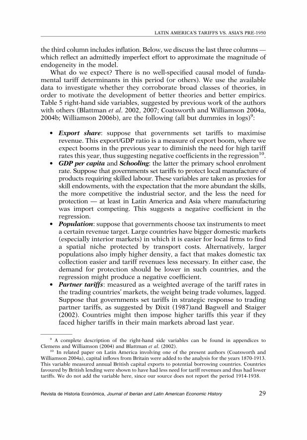
Combined, variance in the regressors of Table 5 explains 65-78 per cent ofvariance in the world cross-sectional tariff before 1914. What about thedifferences between Latin America and Asia? The first six columns of Table 6are simply the coefficient estimates from Table 5, reproduced withoutmodification. The next two columns give the average values of each regressorin both Latin America and Asia, in natural logarithms; at the bottom, thesame values for the regressand are shown. Of particular note is the similarityof the figures for effective distance, an average of physical distance to the topfive trading partners weighted by exports sent to that partner, multiplied byan index of transportation costs. Asia may have been farther away from thecore, but it was doing more intra-regional trading than Latin America. LatinAmerica had a notably higher share of exports in GDP, a much smalleraverage population, much more railway penetration and a much greaterdegree of tariff autonomy. It was also richer, more schooled, more urban,faced higher tariffs abroad and underwent much higher rates of inflation.

The final six columns are a linear combination of the previous columns.The result is an estimate of the relative contribution of each variable’sassociation with tariffs in explaining the much higher pre-1914 tariffs inLatin America compared with Asia. It is calculated in the following way.First, we take the difference between the average regressor value in LatinAmerica and its value in Asia, from columns (7) and (8). Second, this differenceis multiplied by the corresponding coefficient from the first six columns. Third,this number is divided by the average difference ln(Own Tariff) between thetwo regions during this period (the last row of columns (7) and (8)). For theresulting ratio d, a value of zero means that inter-regional differences in thatregressor have no partial correlation with inter-regional differences in tariffs. Anegative value indicates that inter-regional differences in that regressor have apartial correlation with lower tariffs in Latin America than in Asia, ceterisparibus. For substantial correlates of the broadly higher tariffs in Asia, we arelooking for large positive values in those last two columns.

There are five variables whose differences accord strongly with bothworldwide correlations between tariffs and country traits, and with the largeobserved tariff differential between the regions11. These are population size,railroad penetration, urbanisation, partner tariffs and tariff autonomy.

This pattern in the data accords with, though it does not definitively test,classes of theory that have been important in the literature. Start with the

11 On the other hand, some potential explanations for the difference is not easily corroboratedby these numbers. The export share in GDP and GDP per capita were higher in Latin America thanin Asia, which does not accord with the observed tariff differential between the regions. Differencesin effective distance or schooling rates also do not accord with the inter-regional difference. Therelative importance of the remaining five variables listed in the text are not affected by the inclusionor omission of inflation, nor are they affected by the exclusion of GDP per capita and export share.



TABLE 6WHAT ACCOUNTS FOR THE DIFFERENCE IN TARIFFS BETWEEN LATIN AMERICA AND ASIA BEFORE 1914?

Average regressorvalues:

Fraction of regional differenceexplained:

Coefficient estimates from Table 5 Latin America Asia d ¼Coeff:�ðL:Am: avg:�Asia avg:ÞðL:Am: tariff�Asia tariffÞ

(1) (2) (3) (4) (5) (6) (7) (8) (10) (20) (30) (40) (50) (60)

ln(Exports/GDP) 20.398 20.195 20.384 20.410 21.94 22.96 20.28 20.14 20.27 20.29

ln(GDP/capita) 20.421 20.524 20.506 20.533 7.16 6.59 20.17 20.21 20.20 20.21

ln(Population) 20.477 20.430 20.612 20.384 20.605 20.359 8.18 10.0 0.62 0.56 0.79 0.50 0.78 0.46

ln(Partner tariff) 0.436 0.505 0.445 0.407 0.438 0.397 2.71 2.14 0.17 0.20 0.17 0.16 0.17 0.16

ln(EffectiveDist.)

0.086 0.141 20.059 0.029 20.092 0.001 8.09 7.99 0.01 0.01 0.00 0.00 20.01 0.00

ln(Railwaymiles)

0.190 0.141 0.386 0.227 0.388 0.219 7.20 5.72 0.20 0.15 0.40 0.23 0.40 0.23

ln(Schooling) 20.117 0.097 20.264 20.037 20.475 20.244 6.96 6.11 20.07 0.06 20.16 20.02 20.28 20.14

ln(Urbanization) 0.174 0.082 0.292 0.138 0.239 0.070 4.55 3.94 0.07 0.03 0.12 0.06 0.10 0.03

Tariff autonomy 0.760 0.618 0.912 0.795 0.843 0.713 0.918 0.211 0.37 0.30 0.45 0.39 0.41 0.35

Inflation 20.030 0.034 20.037 0.030 2.06 0.486 20.03 0.04 20.04 0.03

Inflation squared 0.003 0.002 0.003 0.002 96.9 224 20.27 20.18 20.27 20.18

ln(Own Tariff) 3.24 1.80

Notes: Coefficient estimates in columns (1) through (6) are taken directly from Table 5. Columns (7) and (8) show the average value of the underlyingregressor before 1914 in Latin America and Asia, respectively, where Latin America includes Argentina, Brazil, Chile, Colombia, Cuba, Mexico, Peru, andUruguay and Asia includes Burma, China, Ceylon, Egypt, India, Indonesia, Japan, Philippines, Siam and Turkey. Columns (10) through (60) takethe difference between columns (7) and (8), multiply this difference by the corresponding coefficient from one of the first six columns and divide by thedifference between average ln(Own Tariff) in Latin America and average ln(Own Tariff) in Asia. This value d can be interpreted as the fraction of thedifference between the two regions’ tariffs that is explained by each regressor. Since tariffs were higher in Latin America, a negative value of d suggeststhat the regressor cannot explain the observed difference; a large positive value suggests it can.

The italics are to show that these are a different kind of number from the numbers in the other columns.

MIC

HA

EL

A.

CL

EM

EN

S/JE

FF

RE

YG

.W

ILL

IAM

SO

N

32R

evis

tade

His

toria

Econom

ica,

Journ

alof

lberia

nand

Latin

Am

eric

an

Econom

icH

isto

ry

first three variables, saving tariff autonomy and partner tariffs for last. Asia’senormous populations provided gargantuan internal markets in which pro-ducers could exploit specialisation and scale. Large internal markets tendedto diminish the need for tariffs to protect import-competing producers. LatinAmerica’s exploding railroad network certainly increased export sectoraccess to foreign markets, but it also exposed interior producers to moreforeign competition, encouraging a tariff backlash to offset the impact of therailroads. The railroad system was less extensive in Asia, and in fact we havemeasured it in a fashion that understates the Asian railroad shortfall (milesof railway trunk line, rather than miles per capita). A less extensive railwaysystem in Asia implied less need for tariffs for protective purposes. It is alsoargued that Asian railroads were built primarily to foster exports, illustratedby Hurd’s (1975) study of India.

Higher levels of urbanisation in Latin America also accord with the gap intariff rates between Latin America and Asia under these partial correlations.Rogowski (1989) has used the Stolper–Samuelson theorem to suggest thatwe look to Latin American urban capitalists for the political economyexplanation for those extraordinarily high tariffs during the belle epoque.Although their economies certainly varied in labour scarcity, every LatinAmerican country faced relative capital scarcity and relative land abundance.As the Stolper–Samuelson theorem has it, «protection benefits (and liberal-ization of trade harms) owners of factors in which, relative to the rest of theworld, that society is poorly endowed» (Rogowski 1989, p. 3). According tothis kind of thinking, urban capitalists should have been looking to formprotectionist coalitions as soon as the Latin American belle epoque and thepax britannica globalisation forces began to threaten them with freer trade.High urbanisation rates in Latin America gave these interests more power toachieve protection, while low rates in Asia contributed to the opposite result.

Even controlling for so many other factors, tariff autonomy is still associatedwith higher tariffs. How much did it matter? After all, we have seen a variety oftariff rates even within colonies run by imperialists favouring free trade at home.Yet, policy autonomy implied high tariffs before WW1, with the coefficient on theautonomy variable in the regressions ranging between 0.618 and 0.912 in col-umns (1) through (6). The model suggests, then, that tariff autonomy might havebeen associated with higher tariffs by a factor of 1.7-2.5, all else equal12. That is,tariff autonomy per se for late 19th century Asia is predicted to correlate with anincrease in average Asian tariffs from 7 to 17 per cent. Turning to columns (10)through (60), we see that Asia’s lack of tariff autonomy accounts for about one-third of the tariff difference between Asia and Latin America. However, thatleaves almost two-thirds associated with factors other than tariff autonomy.

Did the Asian countries subjected to unequal treaties, but not formallycolonies (China, Japan and Siam), have higher tariffs than those that were

12 Since the dependent variable is in logs, 0.618 3 2.72 5 1.68 and 0.912 3 2.72 5 2.48.



colonies (Burma, Ceylon, India, Indonesia and the Philippines)? Surpris-ingly, they did not, as Figure 3 documents.

With policy autonomy, moving naively along these partial correlations,hypothetical Asian tariff levels might have been half those of Latin America,rather than only a fourth. However, as we have seen, tariff autonomy was notthe only variable showing important associations with tariffs. Internal mar-ket size and the protection of the market that poor railroads offered domesticproducers appear to correlate with lower tariffs. Weak political power of theAsian urban capitalist may also have mattered, a weakness associated withsmaller urban presence there compared with Latin America, though the urba-nisation proxy used here could well correlate with other competing factors.Finally, after controlling for tariff autonomy, partner tariffs correlate stronglywith own tariffs. If your trading partner had high tariffs, so did you. LatinAmerica traded more with protectionist North America, whereas Asia tradedmore with free trade Europe (especially its free trade colonisers Britain and theNetherlands). This suggests an interesting candidate to further explain the tariffgap between the regions, though it by no means settles the issue.

We cannot leave this section without saying a word about historical per-sistence, especially in the case of Latin America. Table 5 covers the four decadesafter 1870, but what about the half century before? Does it seem to matter thatthis post-independence period was extremely violent in Latin America?

Customs duties, relative to other sources of revenue, are an inexpensiveway to finance rising central government expenditures on infrastructure anddefence. It is plausible that there might be greater reliance on tariffs than onother sources of revenue in young, recently independent economies with fewbureaucratic resources to implement efficient collection, limited access toforeign capital markets, more enemies and no imperialist protection fromthem. This was certainly true of the newly independent United States andLatin American countries in the first half of the 19th century, although theUnited States had more success in gaining access to European capital mar-kets. As Centeno (1997, Table 1) has shown, the average share of customsduties in total revenues across eleven Latin American republics was 57.8 per centbetween 1820 and 1890. Furthermore, customs revenues are especiallyimportant for land-abundant countries with federal governments since theydo not have the population and taxpayer density to make other forms of taxcollection efficient13. Finally, there was a huge revenue need to bankrollarmed conflict in the United States of the 1860s and the newly independentLatin American republics between the 1820s and the 1870s (see Centeno1997; Mares 2001; Bates et al. 2007).

The preoccupation with national defence and internal security pushed thenewly independent Latin American republics towards higher revenue-generating

13 For federal governments, customs revenues were even bigger share of total revenues in LatinAmerica (65.6 per cent).



tariffs. Centeno (1997) documents that military expenditures quickly rose toconsume over 70 per cent and often more than 90 per cent of all revenues. Weakgovernments, under attack from within and without, abandoned internal taxesthat required an extensive and loyal bureaucracy to collect and concentratedinstead on tax collection at a few ports and mines. Thus, levels of tariff pro-tection rose in every Latin American country (for which there are data) as didthe customs revenues as a percentage of total government revenues.

We stress these facts since we believe that historical persistence matters,and that some part of those very high Latin American tariffs between 1870and WW1, can be explained by the level of violence in the half century before1870, violence so particular to Latin America during what was otherwise apax britannica world.

7. WHAT EXPLAINS THE INTERWAR RISE IN ASIAN PROTECTION?

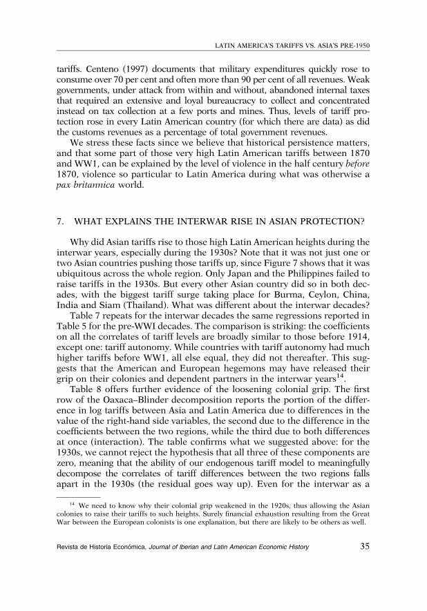
Why did Asian tariffs rise to those high Latin American heights during theinterwar years, especially during the 1930s? Note that it was not just one ortwo Asian countries pushing those tariffs up, since Figure 7 shows that it wasubiquitous across the whole region. Only Japan and the Philippines failed toraise tariffs in the 1930s. But every other Asian country did so in both dec-ades, with the biggest tariff surge taking place for Burma, Ceylon, China,India and Siam (Thailand). What was different about the interwar decades?

Table 7 repeats for the interwar decades the same regressions reported inTable 5 for the pre-WWI decades. The comparison is striking: the coefficientson all the correlates of tariff levels are broadly similar to those before 1914,except one: tariff autonomy. While countries with tariff autonomy had muchhigher tariffs before WW1, all else equal, they did not thereafter. This sug-gests that the American and European hegemons may have released theirgrip on their colonies and dependent partners in the interwar years14.

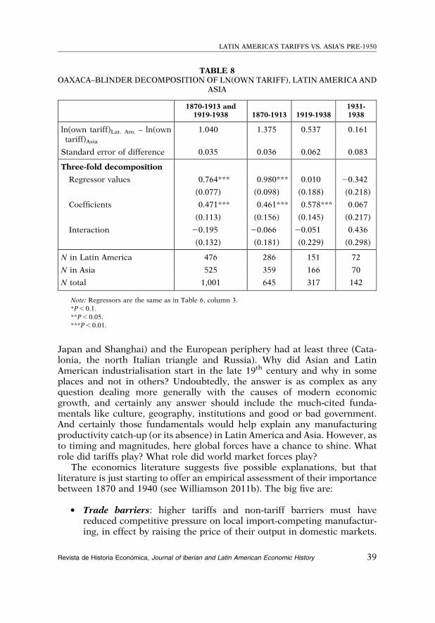
Table 8 offers further evidence of the loosening colonial grip. The firstrow of the Oaxaca–Blinder decomposition reports the portion of the differ-ence in log tariffs between Asia and Latin America due to differences in thevalue of the right-hand side variables, the second due to the difference in thecoefficients between the two regions, while the third due to both differencesat once (interaction). The table confirms what we suggested above: for the1930s, we cannot reject the hypothesis that all three of these components arezero, meaning that the ability of our endogenous tariff model to meaningfullydecompose the correlates of tariff differences between the two regions fallsapart in the 1930s (the residual goes way up). Even for the interwar as a

14 We need to know why their colonial grip weakened in the 1920s, thus allowing the Asiancolonies to raise their tariffs to such heights. Surely financial exhaustion resulting from the GreatWar between the European colonists is one explanation, but there are likely to be others as well.



whole, it appears that differences in the regressors (e.g. autonomy) are notassociated with the regional tariff gap any more, but rather that differencesin how the regressors are associated with tariffs (the coefficients) mattermuch more.

It seems to us that the moral is this: if we are looking for the historicalorigins of inward-looking and anti-market ISI strategies in much of Asiaduring the post-WW2 period, we should start looking at the interwar transitionof the colonies and dependents to policy autonomy, not just in their responseto the global crisis of the 1930s. As for the historical origins of the post-WW2ISI anti-global and anti-market strategies in Latin America, we need notlook farther than the very high tariffs that prevailed there over the centurybefore 1950.

8. DID TARIFF POLICY INFLUENCE INDUSTRIALISATION IN LATINAMERICA AND ASIA?

In some parts of Latin America and Asia, modern industrialisation startedmore than a century ago. Latin America had two emerging industrial leadersin the late 19th century (Brazil and Mexico), Asia had four (Bengal, Bombay,

FIGURE 7TARIFF LEVELS IN ASIA, 1870-1950

0

25

50

0

25

50

0

25

50

0

25

50

1870 1890 1910 1930 1950 1870 1890 1910 1930 1950

Burma Ceylon

China India

Indonesia Japan

Philippines Siam

Ave

rage

Tar

iff L

evel

Year



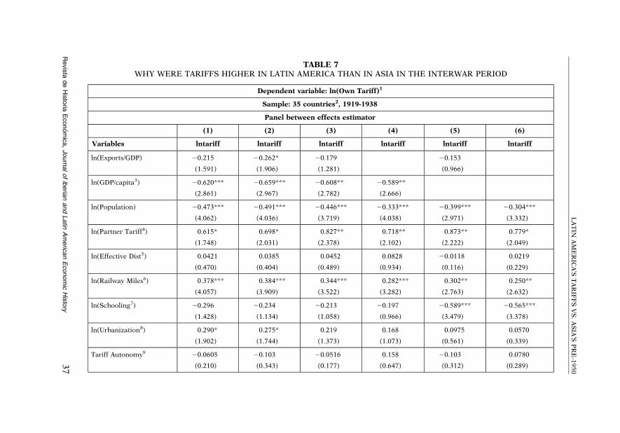
TABLE 7WHY WERE TARIFFS HIGHER IN LATIN AMERICA THAN IN ASIA IN THE INTERWAR PERIOD

Dependent variable: ln(Own Tariff)1



(1) (2) (3) (4) (5) (6)

Variables lntariff lntariff lntariff lntariff lntariff lntariff

ln(Exports/GDP) 20.215 20.262* 20.179 20.153

(1.591) (1.906) (1.281) (0.966)

ln(GDP/capita3) 20.620*** 20.659*** 20.608** 20.589**

(2.861) (2.967) (2.782) (2.666)

ln(Population) 20.473*** 20.491*** 20.446*** 20.333*** 20.399*** 20.304***

(4.062) (4.036) (3.719) (4.038) (2.971) (3.332)

ln(Partner Tariff4) 0.615* 0.698* 0.827** 0.718** 0.873** 0.779*

(1.748) (2.031) (2.378) (2.102) (2.222) (2.049)

ln(Effective Dist5) 0.0421 0.0385 0.0452 0.0828 20.0118 0.0219

(0.470) (0.404) (0.489) (0.934) (0.116) (0.229)

ln(Railway Miles6) 0.378*** 0.384*** 0.344*** 0.282*** 0.302** 0.250**

(4.057) (3.909) (3.522) (3.282) (2.763) (2.632)

ln(Schooling7) 20.296 20.234 20.213 20.197 20.589*** 20.565***

(1.428) (1.134) (1.058) (0.966) (3.479) (3.378)

ln(Urbanization8) 0.290* 0.275* 0.219 0.168 0.0975 0.0570

(1.902) (1.744) (1.373) (1.073) (0.561) (0.339)

Tariff Autonomy9 20.0605 20.103 20.0516 0.158 20.103 0.0780

(0.210) (0.343) (0.177) (0.647) (0.312) (0.289)

LA

TIN

AM

ER

ICA

’ST

AR

IFF

SV

S.

AS

IA’S

PR

E-1950

Revis

tade

His

toria

Econom

ica,

Journ

alof

lberia

nand

Latin

Am

eric

an

Econom

icH

isto

ry37

TABLE 7 (Cont.)

Dependent variable: ln(Own Tariff)1



(1) (2) (3) (4) (5) (6)

Variables lntariff lntariff lntariff lntariff lntariff lntariff

Inflation 0.00423 0.00503* 0.00452 0.00520*

(1.696) (2.056) (1.602) (1.905)

Inflation squared 22.98e–06 23.46e–06 22.61e–06 23.04e–06

(1.066) (1.234) (0.827) (0.972)

Constant 7.078*** 6.841*** 6.252*** 5.932*** 5.530*** 5.276***

(4.609) (4.368) (4.040) (3.834) (3.203) (3.096)

Observations 604 585 585 585 585 585

R2 0.630 0.604 0.659 0.635 0.544 0.527

Number of country 35 35 35 35 35 35

Notes: Absolute value of t-statistics is in parentheses below coefficient estimates.*Significant at 10%.**Significant at 5%.***Significant at 1%.1Import duties over imports.2Argentina, Australia, Austria–Hungary, Brazil, Burma, Canada, Ceylon, Chile, China, Colombia, Cuba, Denmark, Egypt, France, Germany, Greece,

India, Indonesia, Italy, Japan, Mexico, New Zealand, Norway, Peru, Philippines, Portugal, Russia, Serbia, Siam, Spain, Sweden, Turkey, United Kingdom,United States and Uruguay.

3In 1990 US$.4Index of average tariff levels in top five trading partners weighted by exports going to that partner.5Product of average physical distance to top five trading partners (principal city to principal city) weighted by exports going to that country, and

transportation cost index.6Miles of railway trunk line in country.7Fraction of the population below the age of fifteen that is enrolled in primary school.8Fraction of the population living in agglomerations of greater than 50,000 people.9Indicator variable taking the value 1 if country has the freedom to set own tariff levels independently, or 0 if it does not.

MIC

HA

EL

A.

CL

EM

EN

S/JE

FF

RE

YG

.W

ILL

IAM

SO

N

38R

evis

tade

His

toria

Econom

ica,

Journ

alof

lberia

nand

Latin

Am

eric

an

Econom

icH

isto

ry

Japan and Shanghai) and the European periphery had at least three (Cata-lonia, the north Italian triangle and Russia). Why did Asian and LatinAmerican industrialisation start in the late 19th century and why in someplaces and not in others? Undoubtedly, the answer is as complex as anyquestion dealing more generally with the causes of modern economicgrowth, and certainly any answer should include the much-cited funda-mentals like culture, geography, institutions and good or bad government.And certainly those fundamentals would help explain any manufacturingproductivity catch-up (or its absence) in Latin America and Asia. However, asto timing and magnitudes, here global forces have a chance to shine. Whatrole did tariffs play? What role did world market forces play?

The economics literature suggests five possible explanations, but thatliterature is just starting to offer an empirical assessment of their importancebetween 1870 and 1940 (see Williamson 2011b). The big five are:

> Trade barriers: higher tariffs and non-tariff barriers must havereduced competitive pressure on local import-competing manufactur-ing, in effect by raising the price of their output in domestic markets.

TABLE 8OAXACA–BLINDER DECOMPOSITION OF LN(OWN TARIFF), LATIN AMERICA AND

ASIA

1870-1913 and1919-1938 1870-1913 1919-1938

1931-1938

ln(own tariff)Lat. Am. – ln(owntariff)Asia

1.040 1.375 0.537 0.161

Standard error of difference 0.035 0.036 0.062 0.083

Three-fold decomposition

Regressor values 0.764*** 0.980*** 0.010 20.342

(0.077) (0.098) (0.188) (0.218)

Coefficients 0.471*** 0.461*** 0.578*** 0.067

(0.113) (0.156) (0.145) (0.217)

Interaction 20.195 20.066 20.051 0.436

(0.132) (0.181) (0.229) (0.298)

N in Latin America 476 286 151 72

N in Asia 525 359 166 70

N total 1,001 645 317 142

Note: Regressors are the same as in Table 6, column 3.*P , 0.1.**P , 0.05.***P , 0.01.



NTBs should include real exchange rate manipulation and the greatdepreciations during the interwar decades. In contrast, fallingtransportation costs across sea lanes (effective distance) would haveincreased competitive pressure on home manufacturing, and railroaddevelopment (railway mileage per land area) would have done thesame by exposing internal markets to more foreign competition. Howbig were those effects, and was tariff and exchange rate policy the mostimportant of them?

> Terms of trade and world markets: a secular rise in primary productprices may foster an export boom in the poor periphery — as well as aGDP per capita gain — but it will also cause de-industrialisation. The19th century offers abundant evidence confirming this effect, whetherfor India, Mexico or the Ottoman Empire15. However, if a primaryproduct export price boom fostered de-industrialisation in the poorperiphery, the secular export price slump between the 1870s and 1890sand the 1930s16 should have fostered industrialisation there as well.

> Wage costs: as the poor periphery fell further behind the fast-growingindustrial core up to WW1 — what we now call the Great Divergence —wage costs per unit of labour fell in the poor periphery relative to theindustrial core. Furthermore, since, without the role of trade barriers,manufacturing prices were similar the world around, the own wage inmanufacturing (the nominal wage divided by the price of manufacturingoutput) must also have fallen in the poor periphery relative to the richindustrial core. This rising gap should have given the poor periphery anincreasing cost advantage in their domestic markets, ceteris paribus,fostering industrialisation, led by labour-intensive manufacturing.

> Fuel and intermediate input costs: textile manufacturing needscotton, wool, flax and silk intermediates, but many countries do notgrow some or any of them. Metal manufacturing needs ores, but manycountries do not mine them. Since these are high bulk, low-valueproducts, they were expensive to ship long distance in 1870; however,transport revolutions had lowered those costs dramatically by 1940.Manufacturing in natural resource scarce countries in the poorperiphery must have benefited by global market integration muchmore than did the resource-abundant industrial leaders. In addition,modern steam-driven power in industry needed cheap fuel. Thosewithout coal to mine or oil to pump suffered severe competitivedisadvantage in 1870, but that disadvantage had almost evaporated forany poor periphery country without coal or oil reserves in the moreglobal world of 1940 when they could import the stuff cheaply.

15 For India, see Clingingsmith and Williamson (2008), for Mexico, see Dobado et al. (2008) andfor the Ottoman Empire, see Pamuk and Williamson (2011).

16 As famously noted by Prebisch (1950) and Singer (1950). See also Williamson (2008, 2011b).



> Productivity catch-up: given wage, fuel and intermediate costs, givenworld market conditions and given tariff policy, productivity catch-upof domestic manufacturing on the industrial leaders should surely havefostered industrialisation in the poor periphery. This, one supposes, iswhere the role of pro-growth institutions and good government shouldshine.

While these are the big five, any future analysis should also control fordomestic market size and the level of human capital — required moreintensively in manufacturing than in primary product production — as wellas whether the country was a colony — and thus whether it had autonomyover other than just tariff policy. Other forces might include whether parts ofinterwar Asia were mimicking pro-industrial policies in emerging industrialnew comers like Brazil, Mexico and Russia/USSR.

9. CONCLUDING REMARK

Are there lessons from history here? Perhaps, but we prefer to end insteadwith the following challenge: any claim that liberal trade policy lies at theheart of recent growth performance in these two regions must also explainwhy high tariffs did not dampen growth or industrialisation during the LatinAmerican belle epoque and why low tariffs did not ignite growth or indus-trialisation in Asia before 1914.

REFERENCES

ANDERSON, J. E. (1998): «Trade Restrictiveness Benchmarks». Economic Journal 108(July), pp. 1111-1125.

ANDERSON, J. E., and NEARY, J. P. (1994): «Measuring the Restrictiveness of Trade Policy».The World Bank Economic Review 8 (May), pp. 151-169.

BAGWELL, K., and STAIGER, R. W. (2002): The Economics of the World Trading System.Cambridge, Mass: MIT Press.

BAIROCH, P. (1989): «European Trade Policy, 1815-1914», in P. Mathias, and S. Pollard(eds), The Cambridge Economic History of Europe, vol. VIII. Cambridge: CambridgeUniversity Press, pp. 1-160.

BAIROCH, P. (1993): Economics and World History: Myths and Paradoxes. New York:Harvester Wheatsheaf.

BAIER, S. L., and BERGSTRAND, J. H. (2001): «The Growth of World Trade: Tariffs,Transport Costs, and Income Similarity». Journal of International Economics 53 (1),pp. 1-27.

BATES, R. H.; COATSWORTH, J. H., and WILLIAMSON, J. G. (2007): «Lost Decades: Post-independence Performance in Latin America and Africa». Journal of EconomicHistory 67 (December), pp. 917-943.

BERNHOFEN, D. M., and BROWN, J. C. (2004): «A Direct Test of the Theory of ComparativeAdvantage: The Case of Japan». Journal of Political Economy 112 (1), pp. 48-67.



BERNHOFEN, D. M., and BROWN, J. C. (2005): «An Empirical Assessment of theComparative Advantage Gains from Trade: Evidence from Japan». AmericanEconomic Review 95 (March), pp. 208-224.

BLATTMAN, C., CLEMENS, M. A., and, WILLIAMSON, J. G. (2002): «Who Protected and Why?Tariffs the World Around 1870-1913». Paper presented to the Conference on thePolitical Economy of Globalization, Dublin (August 29-31).

BLATTMAN, C.; HWANG, J., and WILLIAMSON, J. G. (2007): «The Impact of the Terms of Tradeon Economic Development in the Periphery, 1870-1939: Volatility and SecularChange». Journal of Development Economics 82 (January), pp. 156-179.

BULMER-THOMAS, V. (1994): The Economic History of Latin America Since Independence.Cambridge: Cambridge University Press.

BRANDT, L. (1993): «Interwar Japanese Agriculture: Revisionist Views on the Impact ofthe Colonial Rice Policy and Labor-Surplus Hypothesis». Explorations in EconomicHistory 30 (3), pp. 259-293.

CENTENO, M. A. (1997): «Blood and Debt: War and Taxation in Nineteenth-Century LatinAmerica». American Journal of Sociology 102 (May), pp. 1565-1605.

CLEMENS, M. A., and WILLIAMSON, J. G. (2004): «Why Did the Tariff-Growth CorrelationReverse After 1950?». Journal of Economic Growth 9 (March), pp. 5-46.

CLINGINGSMITH, D., and WILLIAMSON, J. G. (2008): «De-Industrialization in 18th and 19th

Century India: Mughal Decline, Climate Shocks and British Industrial Ascent».Explorations in Economic History 45 (July), pp. 209-234.

COATSWORTH, J. H., and WILLIAMSON, J. G. (2004a): «The Roots of Latin AmericanProtectionism: Looking Before the Great Depression», in A. Estevadeordal,D. Rodrik, A. Taylor, and A. Velasco (eds), Integrating the Americas: FTAA andBeyond. Cambridge, Mass: Harvard University Press, pp. 37-74.

COATSWORTH, J. H., and WILLIAMSON, J. G. (2004b): «Always Protectionist? Latin AmericanTariffs from Independence to Great Depression». Journal of Latin American Studies36 (part 2, May), pp. 205-232.

CORBO, V. (1992): «Development Strategies and Policies in Latin America: A HistoricalPerspective». International Center for Economic Growth, Occasional Paper no. 22(April) pp. 16-48.

ESTEVADEORDAL, A.; FRANTZ, B., and TAYLOR, A. M. (2003): «The Rise and Fall of WorldTrade, 1870-1939». Quarterly Journal of Economics 118 (May), pp. 359-407.

DIAZ-ALEJANDRO, C. (1984): «Latin America in the 1930s», in R. Thorp (ed.), Latin Americain the 1930s. New York: Macmillan, pp. 17-49.

DIXIT, A. (1987): «Strategic Aspects of Trade Policy», in T. F. Bewley (ed.),Advances in Economic Theory: Fifth World Congress. New York: CambridgeUniversity Press.

DOBADO, R.; GOMEZ-GALVARRIATO, A., and WILLIAMSON, J. G. (2008): «Mexican Exception-alism: Globalization and De-Industrialization 1750-1877». Journal of EconomicHistory 68 (September), pp. 758-811.

GERSCHENKRON, (1943): Bread and Democracy in Germany. Berkeley, Cal: University ofCalifornia Press.

GOMEZ-GALVARRIATO, A., and WILLIAMSON, J. G. (2009): «Was It Prices, Productivity orPolicy? The Timing and Pace of Industrialization in Latin America 1870-1910».Journal of Latin American Studies 41 (December), pp. 663-694.

HOWE, C. (1996): The Origins of Japanese Trade Supremacy. Chicago: University ofChicago Press.

HUBER, J. R. (1971): «Effect on Prices of Japan’s Entry into World Commerce after1858». Journal of Political Economy 79 (3), pp. 614-628.



HURD, J. (1975): «Railways and the Expansion of Markets in India, 1861-1921».Explorations in Economic History 12 (3), pp. 263-288.

INGRAM, J. C. (1971): Economic Change in Thailand 1850-1970. Stanford, California:Stanford University Press.

JACKS, D.; O’ROURKE, K. H., and WILLIAMSON, J. G. (2011): «Commodity Price Volatilityand World Market Integration since 1700». Review of Economics and Statistics93 (3), pp. 800-813.

KANG, K. H., and, CHA, M. S. (1996): «Imperial Policy or World Price Shocks? ExplainingInterwar Korean Living Standards». Paper presented to the Conference on East andSoutheast Asian Economic Change in the Long Run, Honolulu, Hawaii (April).

KINDLEBERGER, C. P. (1951): «Group Behavior and International Trade». Journal ofPolitical Economy 59 (February), pp. 30-46.

LEHMANN, S., and O’ROURKE, K. H. (2011): «The Structure of Protection and Growth inthe Late 19th Century». Review of Economics and Statistics 93 (2), pp. 606-616.

LINDERT, P. H., and WILLIAMSON, J. G. (2002): «Does Globalization Make the World MoreUnequal?», in M. Bordo, A. M. Taylor and J. G. Williamson (eds), Globalization inHistorical Perspective. Chicago: University of Chicago Press and NBER.

LOCKWOOD, W. W. (1968): The Economic Development of Japan: Growth and StructuralChange. Expanded Edition. Princeton: Princeton University Press.

MARES, D. (2001): Violent Peace: Militarized Interstate Bargaining In Latin America.New York: Columbia University Press.

NUNN, N., and TREFLER, D. (2010): «The Structure of Tariffs and Long-Term Growth».American Economic Review: Macroeconomics 2 (4), pp. 158-194.

O’ROURKE, K. H. (2000): «Tariffs and Growth in the late 19th Century». EconomicJournal 110 (April), pp. 456-483.

O’ROURKE, K. H., and WILLIAMSON, J. G. (1999): Globalization and History. Cambridge,Mass: MIT Press.

O’ROURKE, K. H., and WILLIAMSON, J. G. (2002): «After Columbus: Explaining the EuropeanOverseas Trade Boom 1500-1800». Journal of Economic History 62 (June), pp. 417-456.

PAMUK, S- ., and WILLIAMSON, J. G. (2011): «Ottoman De-Industrialization 1800-1913:Assessing the Shock, Its Impact and the Response». Economic History Review 64(February Special Issue), pp. 159-184.

PREBISCH, R. (1950): The Economic Development of Latin America and Its PrincipalProblems. Lake Success, NY: United Nations, Department of Economic Affairs.

POELHEKKE, S., and VAN DER PLOEG, F. (2007): «Volatility, Financial Development and theNatural Resource Curse». CEPR Discussion Paper 6513, Centre for Economic PolicyResearch, London (October).

OWEN, R. (1993): The Middle East in the World Economy 1800-1914. London: Tauris.REMER, C. F. (1926): The Foreign Trade of China. Shanghai: The Commercial Press Ltd.ROGOWSKI, R. (1989): Commerce and Coalitions: How Trade Effects Domestic Political

Arrangements. Princeton, N.J.: Princeton University Press.SACHS, J. D., and WARNER, A. (1995): «Economic Reform and the Process of Global

Integration». Brookings Papers on Economic Activity, I. Washington, D.C.: BrookingsInstitution.

SINGER, H. W. (1950): «The Distribution of Gains between Investing and BorrowingCountries». American Economic Review 40, pp. 473-485.

TAYLOR, A. (1998): «On the Costs of Inward-Looking Development: Price Distortions, Growth,and Divergence in Latin America». Journal of Economic History 58 (March), pp. 1-28.

VAN DER PLOEG, F. (2011): «Natural Resources: Curse or Blessing?». Journal of EconomicLiterature 49 (2), pp. 366-420.



WILLIAMSON, J. G. (2002): «Land, Labor and Globalization in the Third World, 1870-1940».Journal of Economic History 62 (March), pp. 55-85.

WILLIAMSON, J. G. (2006a): Globalization and the Poor Periphery Before 1950. Cambridge,Mass: MIT Press.

WILLIAMSON, J. G. (2006b): «Explaining World Tariffs 1870-1938: Stolper-Samuelson,Strategic Tariffs and State Revenues», in R. Findlay, R. Henriksson, H. Lindgren andM. Lundahl (eds), Eli Heckscher, 1879-1952: A Celebratory Symposium. Cambridge,Mass: MIT Press.

WILLIAMSON, J. G. (2008): «Globalization and the Great Divergence: Terms of TradeBooms and Volatility in the Poor Periphery 1782-1913». European Review ofEconomic History 12 (December), pp. 355-391.

WILLIAMSON, J. G. (2011a): Trade and Poverty: When the Third World Fell Behind.Cambridge, Mass: MIT Press.

WILLIAMSON, J. G. (2011b): «Industrial Catching Up in the Third World 1870-1975».NBER Working Paper16809, National Bureau of Economic Research, Cambridge,Mass. (February).

YASUBA, Y. (1996): «Did Japan Ever Suffer from a Shortage of Natural Resources BeforeWorld War II?». Journal of Economic History 56 (3), pp. 543-560.



why were latin america’s tariffs so much higher than … were latin america’s tariffs so much...

Documents