Why England? Demand, Growth and Inequality During theIndustrial Revolution

Nico Voigtländer, Hans-Joachim Voth

Universitat Pompeu Fabra, Barcelona

Abstract:

Why was England first? And why Europe? We present a probabilistic modelthat builds on big-push models by Murphy, Shleifer and Vishny (1989), combinedwith hierarchical preferences. The interaction of exogenous demographic factors(in particular the English low-pressure variant of the European marriage pattern)and redistributive institutions – such as the “old Poor Law” – combined to makean Industrial Revolution more likely. Essentially, industrialization is the result ofhaving a critical mass of consumers that is “rich enough” to afford (potentially)mass-produced goods. Our model is then calibrated to match the main charac-teristics of the English economy in 1750 and the observed transition until 1850.This allows us to address explicitly one of the key features of the British Indus-trial Revolution unearthed by economic historians over the last three decades – theslowness of productivity and output change. In our calibration, we find that theprobability of Britain industrializing is 5 times larger than France’s. Contrary tothe recent argument by Pomeranz, China in the 18th century had essentially nochance to industrialize at all. This difference is decomposed into a demographicand a policy component, with the former being far more important than the latter.

1

1 IntroductionAfter millennia of stagnation, living standards and productivity began to increase rapidlyafter 1750. Britain was the first country to break free from Malthusian constraints,with population size and living standards beginning to grow in tandem [Crafts (1985),Wrigley (1983)]. Over the following 250 years, more and more countries have indus-trialized, first in Europe and North America in the nineteenth century, and in the restof the world since the middle of 20th century. Following Romer (1990) and Rebelo(1991), a large literature has evolved explaining long-term growth patterns. Recently,a new set of theoretical papers has modelled the transition from Malthusian stagnationto sustained growth.1 The question that has received much less attention is the cross-sectional variation in the timing of the transition to sustained growth. What explainsthese differences? Why did some countries industrialize so early, with major economicand political consequences that are still felt today? In this paper, we attempt to an-swer this question by modelling the transition from traditional production to advancedtechniques in one country, and then calibrate the model with historical data.

We focus on the interplay of random events and structural factors that facilitatedindustrialization. This is in sharp contrast to recent models of the Industrial Revolu-tion. The transition from stagnant living standards to self-sustaining growth is often in-evitable, given the properties of the pre-industrial world. Hansen and Prescott (2002),for example, assume that exogenously driven technological change in the ‘modern’sector will eventually lead to a shift in production techniques. For much of the latemedieval and early modern period, growth occurred repeatedly during sustained ex-pansions in many countries [Braudel #]. Most of these episodes sooner or later groundto a halt. Some highly advanced economies went into decline – with the Italian Re-publics the most prominent case – while others like Holland stagnated at a high levelof income. What explains these stops and starts? Taking our cue from earlier work byCrafts (1977) and by Acemoglu and Zilibotti (1997), our model takes the probabilisticnature of the transition to self-sustaining growth into account. Crucially, we calibrateour model using historical data to obtain quantitative estimates of the industrializationprobabilities for various countries.

Instead of assuming exogenously given or population-driven innovations, we em-phasize structural change.2 Starting with the observation that many new techniquesand manufacturing procedures had been available for some time, we are argue thatadoption, not new inventions drove the industrialization process for most of its earlyperiod, from 1750-1850. It is change during this crucial period that we are attemptingto explain.

We employ a “big push” model, and combine it with hierarchical preferences amongstconsumers in the tradition of Murphy et al. (1989a) . Our model consists of two groups

1Prescott and Moav (2002); Galor and Weil (2000); Jones (2001).2In this sense, our paper pursues a modelling approach that is the logical opposite of Hansen and Prescott

(2002).

2

of consumers – rich and poor – and three production sectors – agriculture, manufactur-ing and intermediate products. Initially, poor consumers cannot afford manufacturedgoods; they consume solely food products, while the rich have access to manufac-tured goods and food. Random, positive shocks to agricultural productivity can raisemass incomes and permit the poor to consume manufactured goods – the higher theirstarting incomes are, the greater the likelihood. The key element for adoption of theconstant-returns-to-scale (“Solow”) technology with relatively high fixed costs is suf-ficient demand. The increased demand for manufactured products then makes it prof-itable for manufacturing firms to sink the up-front costs necessary for industrialization.We add an intermediate goods sector to capture some of the salient features of the In-dustrial Revolution as it occurred in England. Eventually, with enough manufacturingfirms using advanced techniques, the intermediate products sector also industrializes.This allows us to explain the fact that steam engines (intermediate inputs) were widelyadopted in England only a century after their invention, whereas innovations such as thespinning jenny and the Arkwright frame (used in manufacturing) had a much shorteradoption time span (Crafts 2004#).

One key determinant of effective demand was inequality. We follow the lead byZweimüller (2000); Murphy et al. (1989a) and Foellmi and Zweimüller (2004), whoused hierarchical preferences and inequality in growth models. The limiting factor inour model is the purchasing power of the poor rather then overall size of the market.3England had higher consumption levels because of its favorable demographic regimeand unusually generous welfare system. These factors made industrialization morelikely but didn’t determine the outcome. Our approach allows us to model the problemof “why England?” in an explicitly probabilistic setting (Crafts 1977). Country-specificfactors determine whether the switch from advanced techniques occurs at all, and withwhat likelihood.

This setup allows us to make sense of a number of peculiarities that have oftenbeen raised in the context of England’s early transition to self-sustaining growth. Thefinding of slow growth after 1750 implies that living standards must have already beenrelatively high already at this point in time. This was largely a result of a favorabledemographic regime. Europeans in general enjoyed higher per capita living standardsduring the early modern period than their Asian, African and Latin American peers.4The key reason was the ‘European marriage pattern’ – the fact that West of a line fromSt. Petersburg to Triest, age at first marriage for women was determined by socioeco-nomic conditions, not age at first menarche. England in particular was characterizedby a low-pressure demographic regime – negative shocks to income were mainly ab-sorbed by falls in fertility rather than increases in mortality [Wrigley and Schofield(1981); Wrigley et al. (1997)]. This stabilized per capita living standards and avoidedthe waste of resources and human lives that come from the operation of the ‘positive’Malthusian check, when population declines because of widespread starvation.

3In our model, consumption by the rich is not sufficient for industrialization to get under way.4Pomeranz 2000 has recently argued that, for the Yankzi region, living standards were broadly similar

with the most advanced regions in Europe. We nonetheless assume that European living standards werehigher – China as a whole could probably not rival the European average (Maddison 2003). Also, recentwork by Broadberry and Gupta (2005) has shown that Pomeranz’s claims, even for the Yankzi area, areprobably exaggerated.

3

In addition, eighteenth-century England had a relatively generous early form ofwelfare. The Old Poor Law (or the ‘Speenhamland system’, as it was known) providedrelatively generous outdoor relief for the rural poor, helping to stabilize their incomes.High per-capita income matters because our model uses hierarchical preferences. SinceEuropeans had higher incomes (and within Europe, Englishmen had the highest percapita living standard), they could afford a greater number of non-agricultural goods.This helps us to sidestep the potential problem for demand-based endogenous growthmodels of the Industrial Revolution noted by Crafts (1995) – that the cross-sectionalevidence seems at variance with the timing of the transition, with France having amuch larger GDP than the UK but a markedly later start. In our model, countries needto have sufficient demand for one or more higher-ranked goods to make adoption ofthe new technology feasible. In this way, there is a trade-off between higher per capitaincome and total GDP. Put differently – England may have been first because its percapita income was close to Dutch levels (where population was markedly smaller),while being much richer than the French (with a much greater population).

The papers that are closest in spirit to ours are Murphy et al. (1989b) and Ace-moglu and Zilibotti (1997). They focus on project indivisibilities and the problem ofdiversifying away risks at an early stage of development. In the beginning, with low percapita living standards, the range of feasible projects in their model is severely limited.Chance in their model is crucial because a run of “good years” increases the probabilityof switching to high-productivity projects. Our model differs in terms of the mecha-nism that allows the switch to new technologies. We also emphasize indivisibilities,but focus on minimum efficient size considerations which require mass consumptionfor profitable adoption of advanced techniques. We also assume that financing is freelyavailable.

Another important literature that relates closely to our work was pioneered byGilboy (1932), who argued that a surge in additional demand in the eighteenth centurycontributed to the British Industrial Revolution. This work has been severely criticizedby Mokyr (1977) and Crafts (1985), and been defended by Ben-Shachar (1984). Ourmodel gives a rigorous formulation to the link between demand and industrializationwithout relying on any of the questionable assumptions that Gilboy made about thetiming of changes in demand. We also do not need to resort to the idea that exogenouschanges in taste altered the labor-leisure trade-off, as suggested by Jones (2001).

We proceed as follows. Section II discusses some of the historical evidence andoffers a broader motivation for the paper. Section III presents our model and derives thebasic properties of the pre-industrial and the industrialized equilibrium. In an exercisesimilar in spirit to Stokey (2001), we calibrate our model with the available data fromBritain in Section III. Section IV presents some alternative specifications for other partsof the globe – namely China and France – in an attempt to derive predictions about therelative probabilities of industrialization. Section V concludes.

2 Motivation and Historical EvidenceThis paper is an attempt to bridge the gap between two literatures. The Industrial Revo-lution, as modelled in a string of recent theoretical papers, shares few similarities with

4

the one uncovered by economic historians over the last two decades [Voth (2003)].The former stress the discontinuous nature of economic change as a result of the tran-sition from ‘Malthus to Solow’ [Hansen and Prescott (2002); Jones (2001)], comparedto centuries of stagnation beforehand. Time is commonly measured in millennia, andeconomic development occurs in the world as a whole [Jones (2001), Galor and Moav(2002)]. Viewed from the perspective of the last few millennia of world history, theIndustrial Revolution is indeed a sharp discontinuity with immediate consequences,affecting most parts of the globe relatively quickly.

The new orthodoxy in economic history, in contrast, has emphasized the slow, grad-ual nature of change. With every set of revisions over the last 20 years, growth ratesof output and productivity have been reduced (Table 2). They are now anything butimpressive even compared to earlier periods of economic history. Instead of a rapidbreak with Malthusian fetters, the most ‘revolutionary’ aspect of the Industrial Rev-olution lies in structural change (Crafts and Harley 1992#). What is also remarkableabout the period after 1750 is not growth or TFP performance as such, but the fact thataccelerated population growth coincided with stagnant or slowly growing wages andoutput per head [Mokyr (1999)].

Table 1: Output and productivity growth during the Industrial RevolutionFeinstein 1981 Crafts 1985 Crafts and Harley 1992 Antras and Voth 2003

Output1760-1800 1.1 1 11801-1831 2.7 2 1.91831-60 2.5 2.5 2.5Productivity1760-1800 0.2 0.2 0.1 0.271801-1831 1.3 0.7 0.35 0.541831-1860 0.8 1 0.8 0.33

A number of important stylized facts are not well accounted-for in current mod-els of the Industrial Revolution. First, the nature of pre-industrial growth is oftenill-defined. Under Malthusian conditions, increases in technology should not lead tolong-run changes in living standards. Many authors therefore assume that an accumu-lation of positive and unexplained shocks will eventually push living standards beyonda threshold, fertility falls and growth in per capita terms takes off as a result. Sec-ond, the probabilistic nature of the Industrial Revolution has been given scant regard.Most models assume that, given the rate of knowledge accumulation, growth in hu-man capital or technological change, the transition from ‘Malthus to Solow’ had tooccur sooner or later. We present a model in which industrialization may occur, butneed never happen at all. Connected with this, there should be scope for periods ofepisodic growth before the transition to rapid per capita income gains. The history ofeconomic growth before 1750 suggests numerous periods of ‘false starts’, when someareas showed proto-industrialization and a move into sectors outside agriculture at atime of temporarily higher living standards – but without providing the basis for a sus-tained period of growth. This also permits us to understand why some areas, despite

5

showing signs of promise for some of their history, failed to industrialize. Fourth, theissue of changes in sectoral composition needs to be separated from the rate of tech-nological change. While most papers analyzing the Industrial Revolution in a long-runperspective implicitly assume that the adoption of new techniques is synonymous witha shift in employment, the history of the British Industrial Revolution suggests theopposite. Growth in employment outside agriculture was not synonymous with broad-based adoption of revolutionary new techniques. Fifth, we should have something tosay about processes occurring over decades, and not only centuries. While the abruptnature of the Industrial Revolution is undisputed when viewed in the context of the lastten millennia, we aim to provide a theoretical structure that helps us understand changeover the medium term.

Britain was an unequal society, even at a relatively early stage of development [Lin-dert and Williamson (1982), Lindert (2000)]. Nonetheless, average British standardsof consumption were relatively high compared to the French, with a much higher mini-mum level of consumption. Fogel (1993) estimated that as a result of higher inequalityand lower per capita output, the bottom 20-30 percent of the French population didnot receive enough food to work productively. While the vast majority of industrialgoods was purchased by the English well-to-do, the poor continued to have access toa significant share of industrial output (Table 2). Even during the 1790s, when foodprices were high, up to 30% of working class budgets continued to be spent on non-food items (with 6% going on clothing). With most of the goods produced by thenascent modern sector having high income elasticities of demand (in excess of 2.3),even modest gains in real wages translated into markedly higher purchases of luxurygoods. One factor that facilitated the non-food expenditure of poorer groups of soci-ety was redistributive policies. The Old Poor Law was an unusually generous formof redistribution. At its peak, transfers amounted to 2.5% of British GDP, and more11% of the population received some form of relief. This may also have had indirecteffects for the wages of those who were not recipients, by reducing competition in thelabor market (Boyer 1990). Finally, because of the large absolute value of the own-price elasticity of non-food spending (of –1.8 amongst the English poor), productivityincreases and subsequent price reductions facilitated the growth of the modern sector[Horrell (1996)].

Table 2: Domestic demand in the UK for manufactured goods1700 1760 1780 1801 1831 1851

Absolute values(mio. sterling) capitalists 6.9 7.1 18.1 26.5 84.8 121.7

workers 3 4.8 6.5 13 18.7 30.9Proportions(%) capitalists 70 60 74 67 82 80

workers 30 40 26 33 18 20Source: Crafts (1985), p. 136

6

3 The ModelConsider a continuum of infinitely-lived agents i ∈ [0, N ], where N indicates popula-tion size. Each consumer is endowed with one unit of labor that he supplies inelasticallyin each period. A fraction ρ of agents is poor (p), and the corresponding share 1− ρ isrich (r). There is a range J ⊂ R+ of final product sectors, each producing one corre-sponding good j ∈ J . In addition, a range Q ⊂ R+ of sectors produces intermediategoods after industrialization. Let Πj denote total profits of industry sector j, and cor-respondingly πj = Πj/N sector j0s profits per person. In this setup, giving πj to eachagent would mean completely equal distribution of sector j0s profits. To introduce in-equality, we define τp,j = πp,j/πj , where πp,j are profits from sector j given to eachpoor person. Consequently, the inequality measure τp,j indicates the profits of sector jgiven to a poor person relative to the profits an average individual receives from sectorj. Similarly, τ r,j = πr,j/πj is the inequality measure for the rich, and it is straightfor-ward to derive τr,j = (1− ρ · δp,j) / (1− ρ) . Note that inequality in the distributionof sector j0s profits is increasing in ρ, provided τ r,j > 1. Total income of an agents inperiod t is then given by Ii,t = wt + τ i,L(rLL/N) +

Rj∈J τ i,jπj,t +

Rq∈Q τ i,mπm,t,

i ∈ {r, p}, where wt is the wage, and the second term reflects the distribution of totalland rents rLL. This equation reflects the underlying assumptions that all agents pro-vide one unit of labor of the same quality, and that the source of inequality betweenrich and poor is the distribution of profits.

3.1 ConsumersConsumers have hierarchic preferences over a continuum [a,∞) of consumption goods,where a is a positive number close to zero. Goods are indivisible and consumption isa take-it-or-leave-it decision. When consuming good j ∈ [a,∞), a consumer derivesmarginal utility 1/j. Thus, the index j captures the hierarchic nature of preferencesby assigning a high marginal utility to low-j (basic needs) goods and a low marginalutility to high-j (luxury) goods.5 Let cp (cr) denote the last good consumed by a poor(rich) agent. Then instantaneous utility takes the form u (ci,t) = ln(ci,t) − ln(a) fori ∈ {r, p}.6 Consequently, the index ci is a welfare measure for agent i. Regardingthe range of consumption, let JA = [a, 1] denote agriculture and food products (in thefollowing referred to as agriculture), and JM = (1,∞) all other, more luxurious goods(for example, manufactured products such as cotton, clothing, or ceramics). In the fol-lowing we will refer to the range JM as manufacturing products. This definition reflectsthe implicit assumption that consumers first satisfy their need for food before movingon to industrial products along the hierarchy of goods. Given disposable income Ii,t,consumers maximize utility in each period, which yields

5This approach is similar to Murphy et.al. (1989) and Zweimüller (2004). Deviating from the former, weuse the interval [a,∞) rather than (0,∞) because this approach enables us to have hierarchic preferencesalso for goods g < 1.

6In this step we need the consumption range [a,∞) rather than (0,∞), since only the former allows usto find a finite value for the integral

R cia

1gdg.

7

ci,t =

½Ii,t/pA

(Ii,t − pA)/pM + 1

, if Ii,t ≤ pA, if Ii,t > pA

(1)

where pA and pM are the price of agricultural and manufacturing goods, respec-tively.7 To keep matters as simple as possible we treat the saving rate as an exogenouslygiven maximum share of total income that is fully or partially utilized whenever up-front costs need to be paid. This point will be explained in more detail below. The setupof the consumption side of the model implies that a final good j ∈ [a, cp] is demandedby every agent in the population, that is, it is demanded by the rich and the poor - fromnow on indexed by the superscript rp. A good j ∈ (cp, cr) is purchased by the richonly - from now on indexed by the superscript r, and finally, goods j ∈ (cr,∞) are notdemanded or produced. This implies the following demand function for final goods

ydj,t ≡

⎧⎨⎩yd,rpj,t =

yd,rj,t =−

N(1− ρ)N

0

, if j ≤ cp, if cp < j ≤ cr

, if j > cr

(2)

3.2 ProducersThe economy’s production side consists of two ranges of final sectors: agriculture andindustry, and a range of intermediate product sectors. Following Murphy et.al. (1989),each final product j ∈ [a,∞) is produced in its own sector, and each sector con-tains two types of firms: First, a competitive fringe of firms with freely accessible pre-industrialization technology and second, a single industrialized firm, provided that thisfirm paid up-front costs Cj to gain access to a higher-productivity industrialized tech-nology. While prices are determined in the competitive fringe, an industrialized firmhas the exclusive access to the advanced technology in its sector and can thus makeprofits due to its lower variable costs (taking prices and demand as given). In orderfor industrialization to be worthwhile in a given sector, expected discounted life-timeprofits after industrialization must exceed the up-front costs.

The competitive fringe in agriculture uses land and labor as inputs in the productionfunction:

fcA¡AA,t, l, n

¢= AA,tl

γpren1−γpreA (3)

where l is land, nA is labor and 0 < γpre < 1. TFP in pre-industrialized agri-culture in period t, AA,t, is calculated as AA,t = (1 + κt)AA where AA is averagepre-industrialized TFP in agriculture and κt is a shock to agricultural TFP following theAR(1) process κt+1 = θκt+εt. Therein, θ is the autocorrelation and εt˜N

¡0, σ2ε

¢. We

choose this representation of the shock since κt can be interpreted as percentage devi-ation from average productivity. The shock should be interpreted as caused by weather

7Strictly speaking, this result is an approximation that is valid if a is sufficiently close to zero and ifpj = pA for all agricultural goods and pj = pM for all manufacturing goods. These conditions will bevalidated later on. Note also that utility maximization of an agent who consumes only agricultural products(i.e., ci,t ≤ 1) implies that the inequality 1/ci,t ≥ pA/pM must hold in order to maintain the hierarchicconsumption pattern. Otherwise, the agent would have an incentive to consume at least one manufacturingproduct (i.e., the first one in the manufacturing range) before finishing the consumption of all food products.

8

conditions rather than changes in technology. The autocorrelation then results from theabundance or shortage of grain in periods following positive or negative shocks.8 Afterpaying up-front cost Fj , j ∈ [a, 1], an agricultural firm gains access to the technology:

fmA

³l, nA, {xq,A}q∈QA

´= AAl

γpostn(1−αA)(1−γpost)A

ÃQAR0

xβq,Adq

!αAβ (1−γpost)

(4)where AA is TFP in industrialized agriculture, 0 < αA < 1 and xq,A is interme-

diate input q taken from a range [0,QA] of available intermediate inputs. There is noshock to industrialized agriculture’s TFP.9 The parameter β ∈ (0, 1) denotes decreasingreturns with respect to each individual intermediate input. Note that both productionfunctions exhibit constant returns to scale with respect to all inputs. However, produc-tion in post-industrialized agriculture is subject to increasing returns with respect tointermediate input variety QA.10

In manufacturing, the competitive fringe uses the technology fcM (n) = AMnM ,where AM is pre-industrialized TFP. After paying Fj , j ∈ (1, cr], a monopolistic firmhas access to industrialized production:

fmM

³nM , {xq,M}q∈QM

´= AMn

(1−αM )M

ÃQMR0

xβq,Mdq

!αMβ

(5)

where AM is TFP in industrialized manufacturing and 0 < αM < 1. The returns-to-scale properties in this production function are the same as those in (3).

Finally, a pre-industrial competitive fringe produces intermediate products with thetechnology f cI (nI) = AInI , where AI is pre-industrial TFP. In the pre-industrial stagethe range of intermediate products that can be produced is restricted to Q ⊂ Q, whichreflects the fact that the more advanced production of intermediate products requiresindustrialized technology. A classical example is the use of steam engines for pumpingwater in coal mines. The payment of FI provides access to the industrialized produc-tion fmI (nI) = AInI , where AI reflects the increased productivity. Under the newtechnology the range of intermediate inputs Q is unrestricted. Note that before in-dustrialization no intermediate products are needed in final goods production and thusQpre = 0. As in agriculture and manufacturing, the price of intermediate inputs isrestricted by the price at which the competitive fringe can produce.

8This fact alone is not sufficient to explain the relatively high autocorrelation of wages (θ = 0.62)observed in the data between 1600 and 1780 in England. As we will argue later, θ picks up the overallstickiness related a shock to agriculture.

9This is a somewhat extreme representation of the fact that industrialized agriculture can react better toweather events such as droughts. However, none of our results (except for the post-industrialized variationof output) depend on this assumption.

10To see this, note that if prices are the same for each intermediate input, xi = x, ∀i, and thus 3 becomesfmA (·) = AAl

γn(1−αA)(1−γ) (QAx)αA(1−γ)Q

1/β

A . For a given total amount of intermediate inputs,QAx, and given land and labor, we then have increasing returns to the variety QA, which is due to thedecreasing returns to each individual intermediate input xi.

9

In our model, industrialization means the wide-spread transition from a largelylabor-input based production towards a higher-productivity production that uses a va-riety of intermediate inputs. Historically, the up-front costs necessary to access thenew technology are related to the purchase of engines (e.g., steam or spinning) andthe erection of the necessary infrastructure, e.g., buildings (Feinstein and Pollard 1988,v.Tunzelmann 1978, Koehn 1995). Intermediate inputs (e.g., coal, cotton or fertilizer)were then used together with labor (and land) to fabricate final products. Note thatthere is no capital in the production functions. In the pre-industrial period, this as-sumption is realistic, as manpower was by far the most important factor of production.In industrialized production, we can think of the up-front costs as being the capitalstock. In this interpretation, firms must erect all production facilities before startingproduction. Moreover, each firm size requires a corresponding up-front investment.Returns to scale, broadly defined (including capital), thus depend on the relationshipbetween up-front costs and firm size. Similarly, returns to capital depend on the formof productivity advance as a function of up-front costs. If this is a convex (concave)function, we have decreasing (increasing) returns to capital.

From now on, we refer to a division J as a collection of similar sectors, i.e., thecollection of all agricultural sectors j = A,∀j ∈ JA, all manufacturing sectors j =M,∀j ∈ JM , and all intermediate sectors q = I,∀q ∈ JI ≡ Q. We assume that withineach division, the available technology is identical across sectors j. Within divisions,sectors then differ with respect to two properties: First, the status of industrializationdetermines whether there is a competitive fringe or one monopolistic firm. This will berepresented in the following by J and Jind, respectively. Second, the number of peopledemanding the sector’s product determines whether it produces for all people or for therich only. This demand-related property will be represented by ω = {rp, r}, denotingrich-poor and rich-only demand, respectively.

3.3 Allocation of Labor and Factor PaymentsThe assumption that all firms in a division have access to the same technology sim-plifies our analysis. We can then reduce the continuum of producers in each divisionJ to four types of representative firms: There are competitive non-industrialized firmsproducing for rich and poor (supplying ys,rpJ ) and producing for rich only (ys,rJ ). In ad-dition, we (potentially) have monopolistic industrialized firms, producing for all con-sumers (ys,rpJ,ind) and others supplying the rich only (ys,rJ,ind). Figure 1 illustrates thedivisions in the economy.11

We normalize the price of agricultural goods to unity. Factor prices for labor andland are then determined in non-industrialized agriculture for the following reasons:First, provided that the condition 1/ci,t ≥ pA/pM holds, agents consume all agricul-tural products along the hierarchy of preferences before going on to the first manu-facturing good. Perfect competition in non-industrialized production then implies thatagricultural firms pay their workers the marginal product of labor and manufacturing

11Figure 1 is showing a simplified case where the line of industrialized sectors is not interrupted by pre-industrial sectors. This however, can be the case since industrialization in our model does not necessarilyproceed along the hierarchy of preferences.

10

Figure 1: An example for the model economy where cp > 1. Some agriculture and somemanufacturing are industrialized.

firms cannot overbid this wage since 1/ci,t ≥ pA/pM . Underbidding is not feasible,either, since then manufacturing workers would shift to agriculture. Second, industri-alized firms have no incentive to pay wages higher then those in the competitive fringe.This holds even if the whole economy is industrialized, which becomes clear if wethink of the competitive fringe as the backup-home-production sector that is used incase that agents find no other employment. Then the wage paid in non-industrializedagriculture is also the reservation wage of agents.12 Due to equivalent factor pricesfor rich-poor and rich-only production and constant returns to scale (provided that allfinal firms use the full amount of available intermediate inputs, Q), goods prices areindependent of the production scale, i.e., pωj = pj , ω = {rp, r}.

There are three types of inputs in this economy: labor, intermediate inputs andland (used in agriculture only). Labor is used in all sectors, but within the divisionsJA or JM there may be different labor allocations across sectors, nrpJ or nrJ , and nrpJ,indor nrJ,ind, depending on whether the sector is producing for all consumers or for richpeople only, and depending on its state of industrialization. In the intermediate sectorlabor demand is nJI or nJI ,ind. Labor is also needed to build infrastructure and ma-chines as sectors industrialize. This type of labor is paid for with the up-front costs,and we have nF = Ft/wt, where Ft is the total up-front cost paid in period t. Finally,the capital stock (i.e., the up-front-costs paid) of industrialized sectors depreciates at δ.Repairing the capital stock requires labor nδ = δKt/wt, where Kt is the total capitalstock in the economy, which corresponds to the sum of all up-front payments up to t insectors that are still industrialized in t. All labor N is used, which yields the resourceconstraint

XJ={JA,JM ,JA,ind,JM,ind}

Xω={rp,r}

nωJmωJ +

XJ={JI ,JI,ind}

nJmJ + nF + nδ = N (6)

where mJ is the mass of sectors in J . As discussed above, firms have increasingreturns with respect to intermediate product variety. This, together with the assumption

12As Feinstein (1998) demonstrated, real wages rose but little until the 1830. This implies that additionaldemand for labor from industrializing sectors was not sufficient to bid up wage rates.

11

that all intermediate firms (and thus prices of intermediate inputs) are identical, impliesthat industrialized final producers (i) use the whole variety of available intermediateproducts, that is, QA = QM = Q and (ii) use identical amounts of each intermediateinput, i.e., xrpq,J,t = xrpJ,t and xrq,J,t = xrJ,t,∀q ∈ Q for J = {JA,ind, JM,ind}. The factthat all intermediate inputs must be used yields the constraint

XJ={JA,ind,JM,ind}

Xω={rp,r}

xωJmωJ = yq (7)

where yq is the output of intermediate sector q, and the condition must hold forall q ∈ Q. If cp < 1, some agricultural sectors produce for the rich only. In thiscase the land rental rates in rich-poor and rich-only agriculture must equalized, whichdetermines the size of land used in the respective sectors, lrp and lr. If an agriculturalsector industrializes, it uses all the land available to the competitive fringe in the sector,that is, if a rich-poor sector decides to industrialize it has lrp > lr at its disposal.Industrializing firms thus take land as exogenously given. All available fertile land Lis used in agriculture, which requires

XJ={JA,JA,ind}

Xω={rp,r}

lωJmωJ = L (8)

3.4 TimingTo keep matters simple, we assume that there is no financial intermediation for poorpeople. Poor agents consume all their income Ip,t in each period as in equation (1).Rich agents provide a maximum share sr of their income Ir,t to finance up-front in-vestments whenever an entrepreneur promises them an expected return rK,j ≥ rK forproject j, i.e., for the industrialization of a firm in sector j. Consequently, the maxi-mum available funds in each period are srIr,t. If no industrialization project promisesa return that exceeds rK , the rich do not invest and consume all their income. Similarly,if only a few projects are regarded worthwhile investing by the rich, they invest a sharesmaller than sr of their income and consume the remainder. The fact that industrial-ization in Europe was initially funded mainly by rich individuals is described, amongothers, in Feinstein and Pollard (1988) and DaRin and Hellmann (2002). Moreover,Crouzet (1965) argues that

"the capital which made possible the creation of large scale ’factory’industries came . . . mainly from industry itself . . . the simple answer tothis question how industrial expansion was financed is the overwhelmingpredominance of self-finance"

In each final sector j, and in each intermediate sector q ∈ Q there is initially a com-petitive fringe producing, and within each fringe there is a potential entrepreneur. Ineach period potential entrepreneurs observe the demand for their sector’s product, fol-lowing the shock to agricultural productivity. However, before undertaking a project,

12

the duration θ of shocks is only known with uncertainty. Optimists believe that a pos-itive shock lasts longer while a negative shock will be over sooner. There is thereforehetereogeneity of beliefs at any one point in time amongst agents about the durationof shocks.13 This attitude means that they expect higher returns to industrializationprojects in their sector. The contrary applies to pessimists. That is, heterogenous en-trepreneurs expect a range of returns rsubjK,j = robjK,j ± 4rK,j , where the objectivelyexpected return robjK,j is calculated using the true value of θ. An entrepreneur in a sectorneeds to borrow money from the rich to finance the up-front costs. If the subjectivelyexpected return to an industrialization project exceeds the rich’s reservation value, i.e.,rsubjK,j ≥ rK , the entrepreneur contacts the rich for lending. The rich have no a-prioriinformation about projects; they have to believe in the entrepreneur’s promised returnrsubjK,j . In return for financing and letting him manage the project, the entrepreneur givesthe rich all property rights of the monopolistic firm that he creates. Once a project isrealized, the entrepreneur learns the actual duration θ of shocks and can thus calcu-late the objectively expected return robjK,j of his project.14 In all subsequent periodshe reports robjK,j to the lenders, and if the objectively expected return falls short of rKfor a consecutive number of periods t > Tl (denoting lenders’ leniency), his effortsare considered as failed and the lenders stop the project, sending the sector back to itspre-industrial state.15 For sectors fallen back to pre-IR, the game with the potential en-trepreneurs starts again. We use the variable Bj,t to track the state of industrializationof all final and intermediate sectors, where Bj,t = 1 if sector j is industrialized andzero otherwise. Following the above discussion, the law of motion for Bj,t is

Bj,t+1 = Bj,t + dBj,t, where (9)

dBj,t =

⎧⎪⎪⎨⎪⎪⎩01−10

if Bj,t = 0 and rK,j,t < rKif Bj,t = 0 and rK,j,t ≥ rK

if Bj,t = 1 and rK,j,et < rK ,∀et ∈ [t− Tl, t]

if Bj,t = 1 and rK,j,et ≥ rK for some et ∈ [t− Tl, t]

(10)

3.5 EquilibriumLet yωj,t denote the output of sector j producing for ω ∈ {rp, r}. We have now com-pleted the setup of the model and can define the equilibrium.

Definition 1 A static equilibrium in period t is a collection of allocations, prices, prof-its, and up-front costs of industrialization project

¡ci,t, Ii,t, n

ωj,t, nq, nF,t, nδ,t, l

ωt , y

ωj,t,

pj,t, xωq,j,t, Q

ωj,t, wj,t, rl,t,Π

ωj,t, F

ωj,t

¢for i = {r, p}, ω ∈ {rp, r}, j ∈ {JA,t, JA,ind,t,

JM,t, JM,ind,t} and q ∈ Qt such that, given the state variables AA,t, Qt and Bj,t,

13In this regard, our model is similar in spirit to Mankiw and Reis (2003).14The assumption of rapid entrepreneurial learning is not crucial for our results, and solely serves to

simplify the model.15This assumption is not only realistic but also necessary in order to avoid one-time extremely negative

shocks to end industrialization of a large proportion of the economy.

13

(i) the choice variable ci,t fulfills equation (1), (ii) final goods markets clear, i.e.,yd,ωj,t = ys,ωj,t = yωj,t,∀j, ω, (iii) agents are indifferent between working in agricul-ture, manufacturing or in the intermediate sector, i.e., wj,t = wt,∀j, (iv) interest ratesin rich-poor and rich-only production must equalize, that is, rrpl = rrl , (v) final produc-ers use the full variety of intermediate inputs,i.e., Qω

j,t = Q,t,∀j, ω, (vi) intermediatesectors are symmetric, that is, pq,t = pI,t and xωq,j,t = xωI,j,t ∀q ∈ Qt and (vii) theresource constraints (6-8) are satisfied.

Definition 2 A dynamic equilibrium is a sequence of static equilibria for t = 0, 1, 2, ...,together with sequences for

©AA,t, Qt, Bj,t

ª∞t=0

, such that, given an exogenous se-quence of shocks to non-industrialized agriculture {εt}∞t=0, and given the initial con-ditions AA,0 and Bj,0, the evolution of the economy satisfies the law of motion inequation (9) and the constraints AA,t ≥ 0 and Qt ≥ 0 in all periods t.

We solve the model by simulation, as described in Appendix A.1. In the followingwe outline the calibration of the model for the industrial revolution in England from1780 to 1850.

3.6 CalibrationWe normalize population, N = 1, and choose land L = 5 such that its rental rate is6%. The share of poor is set to ρ = 85%. This definition follows from the revisedfigures from Massie, as described in Lindert and Williamson (1982), where we includeamongst the "poor" everyone with an income of 40 pounds or less – giving 86% of allfamilies in 1759, with an average income of sterling 22.7. To reflect inequality in profitdistribution we set τp = 0.2 for the distribution of land rents and profits from interme-diate producers and manufacturing. These sectors were mainly in the hand of peoplefalling into the rich category, according to our definition. The corresponding coefficientfor the rich is then τ r = 5.53. These numbers mean that, as compared to an averageagent, a rich person, receives about five times more profits while a poor agent receivesabout one fifth. We choose τp > 0 to reflect the redistribution from rich to poor inEngland’s Speenhamland system. The magnitude is reasonable, considering that withthis calibration our model gives the income of an average rich person as about 2.5 timesthe income of an average poor person in 1780.16 Considering the distribution of profitsfrom industrialized agriculture, we choose a more equal distribution of profits, that is,τAp = τAr = 1. The reason for this choice of parameters is that agriculture was runmainly by poor people who profited when agriculture became more productive. In thesetup of our model, however, wages are determined by the non-industrialized compet-itive fringe in agriculture, so that it does not rise in the progress of industrialization.Therefore, we use the distribution of profits in industrialized agriculture to represent therise in poor people’s income during the industrial revolution. For example, Feinstein’s(1998) estimates suggest that wages increased by 35% between 1780 and 1850.17

16As we also show later, the resulting inequality in consumption produced by our model matches the datawell.

17For the period 1760 to 1850, the increase was only 24% (Voth 2003).

14

Pre-industrial TFP in agriculture has a direct effect on income and, due to the in-equality between rich and poor, on the share of total manufacturing output sold to thesetwo classes of people. This mechanism works as follows: if pre-industrial agriculturalproductivity rises, wages rise, which benefits the poor relatively more than the rich,as their income is mainly composed of wage. If the poor have already finished allfood consumption (i.e., cp > 1), a further rise of income makes the large number ofpoor consume more manufacturing output. Thus, the share of manufacturing productssold to the poor rises. Crafts (1985) gives the percentage of industrial purchases toworkers as about 40% in 1760 and 26% in 1780. We calibrate pre-industrial TFP inagriculture such that about 30% of industrial purchases are made by the poor. The 30%consumption share of the poor imply cp ≈ 1.1 in 1780. We then derive pre-industrialTFP in manufacturing such that for cp = 1: pM = (w/AM ) = pA. This ensures thatthe condition 1/ci,t ≥ pA/pM always holds. We choose initial TFP in pre-industrialintermediate sectors such that it equals TFP in manufacturing.

According to Crafts (2004b, table 1), British labor productivity grew at an aver-age rate of 1.11% per year during the period 1780-1850. Crafts also shows that thisgrowth occurred almost solely in agriculture and modern sectors (cottons, woollens,iron, canals, railways and ships). The share of these sectors in domestic value addedwas about 60% in 1841 (calculated from the input-output table in Horrell et.al. 1994).Assuming that all other sectors (services, housing, public, and defense) did not con-tribute to labor productivity growth, we find that output per worker in agriculture andmodern sectors must have grown at an average annual rate of 1.32%, or a factor ofabout 2.5 between 1780 and 1850.18 We then use this factor to calculate TFP growthin agriculture and modern sectors as described in Appendix A.2.

To derive the magnitude and persistence of shocks in the agricultural sector, weuse real wage data for England 1600-1780 from Wrigley and Schofield (1997). Theunderlying assumption when working with wages rather than output is a strong posi-tive correlation of wages with agricultural productivity before 1780. With fixed laborsupply and agriculture the dominant sector, productivity shocks will have an immediateknock-on effect on real wages in the economy. This is especially true since wages werelargely fixed in nominal terms, and most of the variation in the Phelps-Brown/Hopkinswage series arises from changes in agricultural prices (Wrigley and Schofield 1997).Figure 2 shows the real wage index and its trend.19

From this time series we derive the HP-filtered series of percentage shocks to realwages, i.e., the shocks in the form κt+1 = θκt+εt. We estimate the parameters of thisAR(1) process to be θ = 0.62 (t=10.31) and σε = 0.073. Note that the autocorrelationof shocks is certainly not solely related to weather events, as this could not explain acoefficient of over 0.5. Rather, we think of the autocorrelation as originating from fric-tions within the economy that make shocks keep their influence over several periods.

18There is no agreement in the literature as to whether productivity growth in agriculture was faster, sloweror equal to productivity growth in modern sectors. For example, Crafts (1985: 70-89) shows that productivitygrowth in agriculture was rapid, and in some periods surpassed manufacturing productivity growth. Wetherefore assume that the growth of labor productivity was broadly speaking the same in modern sectors andagriculture.

19The standard deviation of real wages is very similar to the standard deviation of agricultural output inlater years.

15

Figure 2: Real wage index for England 1600-1780 and HP-filtered trend.

However, since pre-industrial agricultural productivity is the only source of fluctuationin our model, we use the above-found autocorrelation to introduce an economy-wideshock.

To calibrate the labor and intermediate input shares of the production functions, weperform some calculations based on the input-output table for 1841 by Horrell et.al.(1994). We explain our methodology in Appendix A.3.

The adoption of steam engine technology is intrinsically related to the industrialrevolution. When calibrating up-front costs in our model we thus refer to costs of steampower adoption.20 Feinstein and Pollard (1982, table 7.6) provide cost figures for steamengines and boilers. Von Tunzelmann (1978, Table 4.2 and Table 4.10) presents figureson additional costs related to engine house, steam pipes, erection and framework forseveral engine sizes and years between 1795 and 1830. Analyzing these numbers, wefind that the ratio of total non-engine cost over the cost of engine and boiler is relativelystable over engine sizes and time at 0.45. We use this number, together with Feinsteinand Pollard’s data on the patent premium charged by Watt and Boulton, to calculatetotal up-front costs of steam engine usage depending on engine sizes. Figure 3 showsour results.

Size and total costs of steam engines are highly correlated, but there is a fixedcomponent in these costs - the intercept is at 337 Pounds. Therefore, average cost perhorsepower falls with engine size. To work with these figures in our model we needtwo further components: First, we derive the average size of steam engines used inEngland during the industrial revolution from Feinstein and Pollard (1982, table 7.5),who provide estimates of the number of steam engines and total horsepower installed

20This approach is also applied by Stokey (2001).

16

Figure 3: Cost of steam engines in England around 1800

in various industrial towns, 1800-1850. Engine sizes there vary between 12 and 29hpwith a weighted average of about 20hp. We consequently assume that the typical in-dustrialized firm in England used engines of 20hp. Our a-priori belief is that only firmsproducing for a broad share of population had incentives to industrialize, whereas therich-only production was in the hands of artisans. Therefore, we assume that an engineof 20hp is needed to shift to industrial production. A sector j that receives demandN can thus be interpreted as producing a product that receives enough regional or in-terregional demand to make a kick-off worthwhile. Note that under this view goodsj can be interpreted to be differentiated by kind and/or region, and N can be seen asa parameter reflecting population density rather than total population. For example, acountry like China with a huge population but also a large surface certainly had severalregional markets for each product.

Second, we need to fit the Pounds or Pounds per hp into the units of our model.Since up-front costs are not included in the production function (e.g., in terms of cap-ital), we cannot use the numbers from Figure 3 directly. What is represented in ourmodel, however, are material costs of industrialized production, i.e., the cost of inter-mediate inputs. Appendix A.4 shows the calculation of total material cost in sectorsproducing for rich and poor, i.e., receiving demand N . Having found these figures,we can relate them to fixed costs using the relation of up-front costs to annual materialcosts in industrial production. Von Tunzelmann (1978, Table 4.11) provides data on up-front costs and annual material cost for 10hp and 30 hp steam engines between 1795and 1835. We use these figures to compute fixed cost and material cost for a hypotheti-cal 20hp engine around 1800 and find the ratio up-front costs over annual material cost

17

φ = 8. Stokey’s (2001) figures suggest a similar ratio of about 8 for 30hp engines.Crafts (2004b) uses the rate of growth of horsepower to calculate the growth rate of thecapital stock. While such an approach works well in a growth accounting exercise, itcannot be applied in our approach, since we explicitly need cost figures. Having foundφ, we can calculate up-front costs for a 20hp engine in the three divisions as

FJ(20hp) = φ · TMCJ(20hp) (11)

where TMCJ denotes total material costs in division J . If a sector producing forthe rich only decided to industrialize, it would not want to use engines as large as thoseused in sectors producing for rich and poor, since its demand is lower. On the otherhand, a sector in another country, supplying more people than the rich-poor Englishsectors, would optimally buy larger engines when industrializing. In order to calculateup-front costs for differently sized engines we run a regression of total cost on enginesize, Cost(hp) = ao + a1·hp, using the data presented in Figure 3. We find bao = 337and ba1 = 68.7 with R2=0.99. Using these estimates and the known value FJ(20hp),we can calculate FJ for different engine sizes.

There are at least two potential biases in our method of calibrating up-front costs:(1) The annual cost of intermediate inputs may overestimate the annual material costfor steam engines as defined in v. Tunzelmann (1978). For example, intermediate in-puts may include products that are not used to run engines but merely to be processed inthe engines. This upward bias would overestimate up-front costs. (2) The cost of pur-chasing and installing steam engines may underestimate real up-front costs of industri-alizing. For example, industrialization may require the complete change of productionlogistics and infrastructure, leading to large costs in addition to purely technologicalcosts. Analyzing whether the former or the latter effect is dominating goes far beyondthe scope of this paper and we leave it open for future research, taking our approach asthe current best guess for finding up-front costs of industrialization.

Due to its lower usage of intermediate inputs, up-front costs in agriculture are lowerthan up-front costs in industry. On the other hand, because of the unfavorable weight-value ratio of most agricultural commodities, few products from the primary sectorcould be marketed throughout the country. We assume that effective market size foragriculture is smaller by a scale factor of υA. There are at least two reasons to believethat υA > 1 is reasonable: First, agricultural products are generally less diversified thanmanufacturing products, so that for the same number of people demanding a product,one expects to have relatively more firms in agriculture supplying this product. Sec-ond, the weight-value ratio is higher for agricultural product, making them relativelymore expensive to transport. Thus, one would expect agricultural markets to be moreregionally bounded, and thus smaller, than markets for manufacturing products. Ourresults are not sensitive to the precise value for υA chosen; we run the calibration withυA = 3, indicating that the market for a manufacturing firm is about three times largerthan for an agricultural firm.

Our calibration of up-front costs yields the following results: FA = 0.63, FM =2.01, and FI = 0.21. We have FM ≈ υAFA, due to the different market sizes.21

21This relation holds only approximately since the intermediate input share are different in agriculture andmanufacturing and because up-front costs per hp are a non-linear function of size (see Figure 3).

18

The up-front costs for the intermediate division are relatively low due to the smallerscale of production in each intermediate sector and the small (hypothetical) share ofintermediate inputs in intermediate goods production. This also has the implicationthat agriculture never industrializes without manufacturing having made the transition.

In order to reflect entrepreneurial heterogeneity with respect to the rate of returnthat they expect for industrialization projects, we use the following figures: 4rK,M =±5% and 4rK,A = 4rK,I ± 2.5%. We draw the subjectively expected return ofan entrepreneur in division J , rsubjK,J , using a uniform distribution over the intervalhrobjK,J −4rK,J , r

objK,J +4rK,J

i. Recall from the discussion above that the hetero-

geneity of entrepreneurs originates from different expectation regarding the durationof shocks. The influence of such shocks is larger in manufacturing than in agricultureor intermediate sectors. The reason for this is that a positive shock raises poor people’sincome, such that the poor demand a wider range of manufacturing products. But oncethe positive shock is over, demand drops back immediately. Now imagine being anentrepreneur in one of the sectors that had only demand from the rich before the shockand receive demand N during the positive shock. As long as demand is high, industri-alized production is highly profitable, but it is less so once the shock is over. Thus, theexpectation of shock duration is crucial in manufacturing. Plugging 4rK,M = ±5%into our model, we find that it is roughly equivalent to expecting an autocorrelation of0.8 for positive shocks and 0.4 for negative shocks (where 0.62 is the correct value).This 25% deviation from the objective duration of shocks seems reasonable.

In agriculture, on the other hand, demand is basically always N , since the simula-tion starts out at cP > 1 (see the above discussion on the calibration of pre-industrialTFP in agriculture). Therefore, the duration of the shock is less decisive than in man-ufacturing, and we choose a smaller heterogeneity for agricultural entrepreneurs. Westill allow for some heterogeneity to reflect other influences like different access to, orspecial tastes for new technology (driving the subjective return up or down). The samearguments apply to the intermediate sector, where a shock also has a relatively smallerinfluence as compared to manufacturing. The demand for intermediate products is de-termined by the state of industrialization in, and the scale of demand for, agricultureand manufacturing products. Since the state of industrialization does not react imme-diately to shocks (recall the discussion regarding leniency of lenders), the expectedduration is not as crucial as in manufacturing.

In order to reflect lenders’ leniency, we choose a maximum of Tl = 3 consecutiveperiods during which the entrepreneur’s expected return can be below the minimumrequired return rK . Finally, we choose the range of intermediate products that can beproduced with pre-industrial technology as Q = 0.1. This is a guess with some under-lying intuition: as explained above, in 1780 our model is calibrated such that cp ≈ 1.1.As a consequence of receiving rich and poor demand, it is already profitable for therange (1, 1.1] of manufacturing sectors to industrialize, although intermediate inputsare not yet produced industrially. We could think of these firms as already being or-ganized in larger units (e.g., manufactories) but not yet using steam power to run theirengines (e.g., using water mills instead). If a range of size 0.1 is producing final prod-ucts with a pretty much industrial technology, a reasonable thing to assume is that asimilar range of intermediate firms is able to produce intermediate inputs for the final

19

production. We therefore choose Q = 0.1. In order to find the maximum share ofincome that rich people are willing to invest, sr, we use the aggregate saving rate s.According to Crafts (1985, p. 95), the average saving rate 1700-1850 was 0.2. The cor-responding investments, however, went into old and new technology, and what we needin our model are investments in the latter, only. Feinstein (1978) showed that net capi-tal formation increased from 7 to 14 percent of GDP. It is reasonable to assume that theincrease in capital formation reflect the investment in modern technology. Using a con-servative estimate, we assume that roughly 5% of GDP was used in capital formationof industrializing sectors by the end of the period, which gives an industrialization-specific investment rate of s = 5%. Recall that only rich people invest in our model.Depending on the share and relative income of poor and rich people, the overall savingrate of 5% translates into a rate sr ≈ 15%. All other parameters used in the modelare fairly standard, and are given in Table 3 together with the calibration we discussedabove.

TABLE 3: Parameter ValuesPopulation and income distribution

N = 1 L = 5 ρ = 0.85 τp= 0.2 τAp = 1TFP

AA= 0.82 AM= 0.94 AI= 0.94 AA= 2.25 AM= 4.36 AI= 2.35Shock to AA

θ = 0.62 σε= 0.073Factor Shares

γpre= 0.3 γpost= 0.3 αA= 0.36 αM= 0.44 αI= 0.27Up-front costs

FA= 0.63 FM= 2.01 FA= 0.21Entrepreneurial Heterogeneity

4rK,A±2.5% 4rK,M= ±5% 4rK,I= ±2.5%Other parameters

δ = 0.05 s = 0.05 β = 0.8 Q= 0.1Tl= 3 rK= 10% υA= 3 φ = 8

4 ResultsIndustrialization in our model is interpreted as the widespread adoption of high-productivitytechnology that depends on intermediate inputs. This process follows various steps.Initially the economy is in its pre-industrial state with agriculture and intermediate in-put production occurring in the low-productivity competitive fringe. For England, ourcalibration yields cP ≈ 1.1 in 1780. Thus, some manufacturing firms receive demandfrom rich and poor people, which makes it worthwhile for them to produce on a largerscale.22 In the language of our model, this means that they sink the up-front costs tobecome monopolists in their sectors and gain access to the technology from equation(5). However, at this stage intermediate inputs are not yet produced industrially, so

22Our calibration of up-front costs yields that for these manufacturing firms the expected return of indus-trilialization is large enough to kick off.

20

that only a small range Q is available, and intermediate inputs are expensive. Histor-ically, these early firms producing at a larger scale can be seen as manufactories runwith water mills and slowly substituting steam power for water. Figures for coal pricesin v.Tunzelmann (1978) support the fact that the price of intermediate inputs droppedsignificantly between 1780 and 1850.

If enough manufacturing firms demand intermediate products, it becomes worth-while for the intermediate sector to industrialize. As shown in Appendix A.1, the priceof intermediate inputs then drops by about 50%. Moreover, it becomes worthwhilefor more intermediate firms to enter the market such that Q grows beyond Q. Thesechanges in the supply of intermediate inputs make industrialization worthwhile in agri-culture, as well as for further manufacturing firms. This, in turn, creates higher demandfor intermediate inputs, which results in a further extension of Q. This process goes onthroughout the transition from the pre- to the post-industrial economy. In the followingwe provide a glance at some features of the pre-industrial economy, i.e., at how theworld in our model would look like without a kick-off; only being driven by shocks toagriculture. Thereafter, we analyze incentives for industrialization in a pre-industrialworld. Finally, we turn to industrialization itself and examine results of our modelregarding the transition period.

4.1 The pre-industrial economySuppose that modern industrial technology had not been available in 1780, then onlythe shock to agricultural TFP would have driven income and consumption, without everinitiating a kick-off. In the following we analyze this hypothetical economy. The upperleft panel of Figure 4 shows income Iω and consumption cω of rich and poor peopleas a result of shocks to agricultural TFP. A remarkable feature is that although therich’s income increases as a result of positive shocks, their consumption scale (i.e., thelast good that they consume along the hierarchy) decreases. The intuition behind thisfinding is that as agricultural TFP increases, wages (that are determined in agriculture)increase and thus the cost of producing manufacturing goods rises.23 Since the largestshare of rich people’s consumption are manufacturing goods, rising prices of thesegoods offset the higher wages. The poor, having the largest part of consumption inagriculture, are less affected by rising prices of manufacturing products and thus profitfrom positive shocks.

The upper right part of Figure 4 shows the composition of GDP. Note that forcp > 1, agricultural output stagnates since all agricultural demand is satisfied. Thebottom left figure shows the composition of the labor force, which compares well withthe data: Crafts (1985, p. 62) suggests that – abstracting from the service sector –31% of the English male labor force were employed in manufacturing in 1760 (with

23Note that to the right of the cp = 1 line, cr grows up to the point where the shock is zero. The reason isthat some low-j manufacturing sectors (i.e., close to 1) are already performing the monopolistic large-scaleproduction, paying profits to the rich. Profits grow with final demand that in turn depends on poor people’sincome, being driven by the shock. The additional income of the rich from profits then is enough to offsetthe rise in manufacturing prices. Due to our restriction of analyzing the non-kick-off economy, no furthermanufacturing firms industrialize in the range of positive shocks, so that the price-effect is the determiningfactor.

21

Figure 4: Features of the pre-industrial economy

linear interpolation, the figure for 1780 is 37%). Finally, the consumption share ofmanufacturing goods are very sensitive to shocks. Variations in the range of ±20%,as seen in Figure 2, let the consumption shares fluctuate between 0 and 50%. Thisvariation is probably too high but not unreasonable, considering the variating shares inTable 2 and the fact that an extremely negative shock to the poor’s income may wellconstrain them to food consumption in that period.

Using the numbers from Table 2, we can perform a plausibility-check of our cal-ibration with respect to inequality in 1780, i.e., the consumption of the rich relativeto the poor. When using ρ = 0.85 for the share of the poor, as used in our calibra-tion, the manufacturing consumption of a representative rich person relative to a poorperson was about 16, according to the data. In our model, we have c1780p = 1.1 andc1780r = 2.58. Since manufacturing goods have index j > 1 , the relative manufactur-ing consumption of rich to poor is 1.58/0.1 = 15.8. This close similarity to the data iscertainly a coincidence; but since it is not a direct result of the calibration, it providesa check for inequality in the model.

22

4.2 Incentives for IndustrializationWe saw above that following a positive shock the range of products consumed by richand poor (cp) increases. But is this sufficient to induce the kick-off of firms? We an-alyze this question in the following, still sticking to the pre-industrial economy. Theleft panel of Figure 5 visualizes the expected returns of industrialization projects underfull information about the duration of shocks. Strictly speaking, we analyze in eachdivision the (objectively) expected returns of the sector that is awaited to industrializenext. These are the lowest-j agricultural sector, an arbitrary intermediate sector, andthe lowest-j manufacturing sector that still has the competitive fringe. We see thatfor manufacturing expected returns are negative for negative shocks and rise sharplyas shocks become positive. The reason for this observation is that industrialization ofmanufacturing is profitable only if rich and poor people demand the product. But forthe sector we look at, this is only the case for positive shocks. The more positive theshock, the longer the time-span over which the objective entrepreneur expects a highdemand, and the higher is his expected return. The demand-profit relation can alsobe seen in the right panel of Figure 5. The distance between price and marginal costof manufacturing production is not changing much with the shock. Thus, the decisivepoint in order to recoup up-front costs must be the amount of output sold.

For agriculture, things look different. The expected return declines with a morepositive shock. The reason for this becomes obvious when looking at prices and vari-able costs of agricultural goods: While pA does not change (numeraire), the variablecosts of industrialized agriculture increase. Intuitively, this follows because wages aredetermined in non-industrial agriculture so that they rise with a positive shock, thusaffecting the labor cost of industrialized agriculture. An alternative explanation is thatthe shock affects only pre-industrial agriculture, while leaving unaffected industrial-ized production (recall the intuition we provided above for industrialized agriculturebeing more capable to cope with weather events). Thus, the relative advantage of in-dustrialized over non-industrialized agriculture diminishes with more positive shocks.The decisive event pushing expected returns of agriculture upwards is not visible inFigure 5 - the drop in intermediate input prices following the industrialization of theintermediate sector. This feature will be analyzed in the next section.

Finally, an intermediate sector charges the mark-up 1/β over its marginal cost.24

Thus, as was the case for manufacturing, demand is the driving force for expected re-turns. However, expected returns in the intermediate sector are less volatile than thosein manufacturing. The explanation is that intermediate sectors’ demand does not de-pend directly on the volatile range of poor people’s consumption, but on the usage ofintermediate products in final production, and thus on the extent of industrialization infinal sectors. This fact becomes obvious in the left panel of Figure 5, where interme-diate profits have a hump just to the left of a zero-shock. This is the range where anegative shock takes away poor people’s final demand from manufacturing, such thatthe monopolistically producing range (1 < j / 1.1) supplies the rich only, thereforedemanding less intermediate inputs. If the shock is negative enough (around -15%),the poor stop all manufacturing consumption, and intermediate entrepreneurs expect

24In Figure 5 we list the price that a monopolistic intermediate producer would charge, not the (higher)price of the competitive fringe.

23

them to return to manufacturing demand only in the far future. An even more negativeshock then matters less for expected profits of intermediate producers.

Figure 5: Incentives for industrialization

Looking again at the left panel of Figure 5, we see that a 30% shock pushes the(objectively) expected return of industrialization in manufacturing above the lenders’constraint rK = 10%. However, due to the entrepreneurial heterogeneity, it is notcompulsory that the expected return passes this level. In fact, extremely optimisticentrepreneurs in manufacturing may already decide to industrialize their sector at ob-jective returns of 5%. Figure 5 shows that this threshold is already passed for shockssmaller than 10%. On the other hand, if in a sector that is expected to kick off next,the entrepreneur is pessimistic, he may require objective returns of up to 15%. Thislevel is never reached within a reasonable range of shocks. Whether or not an indus-trialization occurs thus depends on several factors: (i) a sufficiently positive shock toraise expected returns in manufacturing sectors that are awaited to kick off (i.e., thelowest-j sectors that are not yet industrialized); (ii) a sufficiently optimistic attitude ofentrepreneurs in these sectors; (iii) a sufficiently long duration of the positive shocksuch that enough manufacturing sectors industrialize, creating the demand for the in-termediate sector; (iv) an optimistic attitude of entrepreneurs in the intermediate sectorat the point in time when demand for intermediate products is high.

4.3 IndustrializationIf the previously mentioned four conditions are fulfilled, the economy goes through aperiod of industrialization. Our simulations suggest that there may be failed kick-offsif a positive shock is followed by a long period of negative shocks. If however, indus-trialization reaches the agricultural sector, the process continues even during a series ofnegative shocks. The reason is that, as explained above, the returns of industrializationin agriculture increase with negative shocks to pre-industrial agriculture. In the follow-ing we analyze a typical kick-off by imposing a large enough shock over some periodsand then letting the shock be zero for the remaining time. Figure 6 shows some fea-tures of this ’deterministic’ industrialization. In the upper left panel, a positive shock

24

gives the incentives for manufacturing sectors to kick off. This, in turn, creates demandfor intermediate products so that some periods later the intermediate sector industrial-izes, as well. The resulting drop in intermediate input prices creates incentives forindustrialization in agriculture, which raises the poor’s income. As the poor becomericher, their demand for manufacturing products increases so that more manufacturingfirms industrialize. This process continues until the post-industrialization equilibriumis reached after approximately half a century. This time-span may seem short comparedto the time-span 1780-1850 usually quoted for England’s industrialization. It shouldbe noted, however, that there are no failed kick-offs in this ’deterministic’ simulation,so that all projects are successful, leading to a fast progress. Moreover, our model onlyconsiders the first adoption of modern technology and not its improvement, and thereare no constraints in the model with respect to technology availability. Introducingsuch frictions would enlarge the time-span needed for full industrialization.

The upper right panel of Figure 6 shows that industrialization spreads relativelysmoothly in agriculture and manufacturing, whereas it is a more uneven process forintermediate sectors. Since the size of the industrialized intermediate division is en-dogenous, we derive its optimal extent of industrialization as follows: Whenever it isprofitable for the intermediate division to increase its extent of industrialization, themodel calculates the new range such that the expected returns of each intermediatefirm are 10%.25 Thus, whenever the intermediate division decides to industrialize, theextent of this step depends on how much more demand for intermediate products hasbeen created by agriculture and manufacturing compared to the last time when the in-termediate sector adjusted. This leads to the more uneven industrialization process inthe intermediate division.

Looking at the lower left part of Figure 6 reveals that the inequality between richand poor increases throughout the industrial revolution.26 Recent evidence presentedby Feinstein (1998) suggests that the gains from industrialization primarily accrued tocapital owners. The lower right panel shows the actual return of industrialized firmsproducing for rich and poor. Note that the returns are very smooth, which is due tothe fact that there are no shocks in this analysis. Therefore, the presented returns are abest-case scenario, without demand ever dropping to rich-only for industrialized firms.Manufacturing profits are higher than the others, around 25% as compared to 10%. Butthis is justified because manufacturing firms are much more affected by shocks - so inthe best-case scenario they require higher returns. In fact, when we introduce shocks,the average profits of manufacturing firms are the same as those of the other sectors.The returns of agriculture being around 10% is a result of our calibration of the marketsize parameter υA, while the returns of the intermediate sector follow from the ongoingadjustment of the range of intermediate production.

The left panel of Figure 7 shows GDP and up-front costs paid during the industrial-ization. GDP grows by about 50%, which matches the data well: According to Craftsand Harley 1992, and Crafts 1985, per capita output growth is 1760-1800 is 0.2% p.a.,1800-1830 0.5%, 1830-60, 1.1% . This means an increase of 57% for 1760-1850. Inthe right panel we present the targeted and the actual saving rates of rich investors. The

25The more intermediate firms there are, the smaller is the demand for each firm’s output.26This was originally argued by Williamson (1985), but his evidence was questioned decisively by Fein-

stein (1988).

25

Figure 6: A ‘deterministic’ industrialization

former is the rate at which investors plan their investment at the end of the previous pe-riod, the latter is the actual investment rate when up-front costs are paid. The actual ratemay exceed the target if investment is planned in a period of a positive shock but theshock in the following period is more negative or due to the approximation procedurein our simulation, as explained in Appendix A.1.27 We see that during industrialization,the availability of funds is a binding constraint in each period, at least in the absence ofshocks.

4.4 Probabilities of industrialization in various countriesWhy did the industrial revolution occur in England first? Could it have been France,Belgium or China? In our model, industrialization occurs stochastically, with the prob-ability of a kick-off depending crucially on the initial income and consumption of thepoor. Figure 8 shows the probability of a kick-off occurring in England after 1780,

27We approximate the continuum of sectors by small intervals of width 0.01. Then, for example, if targetedinvestment would be sufficient to let a range of 0.0258 sectors industrialize, we round this number, whichyields 0.03. Actual investment that must be paid for 0.03 then exceeds the targeted investment. As Figure 7shows, however, this approximation does not create large deviations.

26

Figure 7: GDP and savings during the ‘deterministic’ industrialization

given that consumption of rich and poor remains constant at its 1780 level.28 We seethat a kick-off occurring within 50 years after 1780 is very likely.

Figure 8: The probability of a kick-off in England after 1780

In order to compare the kick-off probability in 1780 England with that in othercountries, we would ideally need a cross-section of income, population size, transportcost and income distribution figures. While those available are not of as a high a qual-ity as one might like, we can derive some basic probabilities based on rough estimates.Income data are presented in Table 4.4. We present data on population density, since inthe 18th century transport costs were high so that the population that could be reachedwith reasonable transport effort presumably determined marked size, not merely total

28If we impose an exogenous increase in per-capita consumption, the marginal probabilities of a kick-offin a certain period grow over time.

27

population. At a horizon of 100 years, France in 1780 had an industrialization proba-bility of 20%.29 This is largely the result of a very steep trade-off between populationsize and per capita income – the vast majority of the population in France was so poorthat access to manufactured goods was out of the question. Lower population densitydid not help. In the case of China, population size is essentially irrelevant because theaverage income is so low that industrialization will almost never happen (the probabil-ity is less than 1/1000). Despite the very large number of inhabitants, the number ofrich is never sufficient to enable the move to advanced manufacturing.

The Poor Laws are not important for England’s higher industrialization probability.With redistribution of 2.5% of GDP, "mass incomes" were bolstered at the expense ofthe more privileged groups in society. However, without this redistribution, industri-alization probabilities at a horizon of 100 years are still essentially 100%, even if theprobabilities at shorter horizons are somewhat lower.

TABLE 4: Income and population in other countriesp.c. income (in 1990 Geary-Khamis dollars) Population (mio) Pop. density (per sqm)

Year 1700 1820 1700 1820 1700 1820England 1250 1707 8.56 21.21 37.09 91.88France 986 1230 21.50 31.22 39.09 56.76China 600 600 138 381 14.4 40Sources: Maddison (2001) and CIA (2005) for land area

5 ConclusionWe argue in this paper that combining hierarchical preferences with a big-push modelcan help us understand why England (and Europe) industrialized first. We show that inan economy with minimum fixed capital requirements, the distribution of income, pop-ulation size as well as the average per capita income will influence the probability ofmaking the transition from “Malthus to Solow”. If starting conditions are sufficientlyfavorable, a series of positive shock to agricultural productivity has the potential to startthe industrialization process. It may be interrupted – as growth in early modern Europeoften was – but the right kind of persistent, benign fluctuations will eventually lead towide-spread adoption of new manufacturing techniques. This transition was markedlyeasier in the case of England (and Europe) since starting conditions were unusually fa-vorable. The low-pressure European marriage pattern was crucial in maintaining livingstandards of the wider population at a level that was sufficiently high for them to startconsuming manufactured goods as soon as favorable income shocks occurred. In theEnglish case, the relatively generous Poor Law system also reinforced this effect. Wecalibrate our model with data for England prior to the classic Industrial Revolution, andshow how we can match many of the crucial features isolated by economic historiansin recent decades. We also present quantitative results for the ex ante industrializa-tion probabilities of other countries – in this case, France and China – and show thatEngland’s better chances are largely the result of higher per capita income before the

29The corresponding methodology is presented in Appedix A.5.

28

start of industrialization, which we argue largely reflects more a favorable demographicregime.

29

APPENDIXA.1. Simulating the ModelWe derive the FOC from the production functions for the optimal input of land,

labor, and intermediate inputs in final production. Together with the conditions men-tioned in the definition of the equilibria we simulate the model, finding the static equi-librium for each period and using the laws of motion to go the next period. [Writing ofthis section is work in progress]

A.2. Calibration of Total Factor Productivity Growth

In the following, productivity means output per worker, while total factor produc-tivity (TFP) is simply the A in a production function. As discussed in the sectionCalibration, labor productivity in agriculture and modern sectors grew at a factor of4prd ' 2.5 between 1780 and 1850. In order to find TFP growth we must solve theequation

y1850V A,j

n1850j

= 4prdy1780V A,j

n1780j

(A-1)

for agriculture and manufacturing sectors, using the pre-industrial figures for 1780and the industrialized ones for 1850. In this equation, yV A,j is value added, which isdifferent from total output if intermediate inputs are used, i.e., in industrial production.Equation (A-1) thus becomes

p1780j y1850j −R Q0p1780q x1850q,j dq

n1850j

= 4prdp1780j y1780j

n1780j

(A-2)

where yj denotes total output of sector j. Solving this equation for agricultureyields:

AA =

⎧⎨⎩⎡⎣AA4prd

µγpre

1− γpre

w1780

r1780L

¶γpre µ1− αAαA

p1850I

w1850

¶(1−γpost)αA+

p1780I

p1780A

µ1− αAαA

p1850I

w1850

¶(1−γpost)αA−1⎤⎦"µ 1

Q1850

¶(1−β)αAβ µ1− αAw1850

Ãyrp,1850A

lrp,1850

! 1

(1−γpost)µp1850I

αA

¶αA µ w1850

1− αA

¶1−αA⎞⎠γpost⎤⎦⎫⎬⎭1−γpost

A-3

where we face the problem that while 1780 TFP and thus factor prices are known,1850 variables are endogenously depending on AA. We solve this issue as follows:First, sincew is fixed by non-industrialized agriculture, its expected value is the same in1780 and 1850. Second, the price of intermediate inputs p1850I can be derived from the1850 technology of the intermediate sector, which is known independently of AA (see

30

equation (A-5)). Third, Q1850 can be approximated by its initial value Q. Althoughthis parameter grows larger than Q during industrialization, this approximation is validsince AA reacts inelastically to changes in Q. Finally, to approximate output and landin 1850 we assume that c1850p > 1 such that all agricultural sectors produce for richand poor, which gives output yrp,1850A . Land lrp,1850 is then given by the land use inthe competitive fringe. Solving equation (A-2) for manufacturing implies:

AM =

µ1

Q1850

¶(1−β)αMβ ∙AM4prd

µ1− αMαM

p1850I

w1850

¶αM+

p1780I

p1780Mµ1− αMαM

p1850I

w1850

¶αM−1#(A-4)

where we use the same arguments as above to approximate 1850 variables. Finally,the TFP change in intermediate production can be calculated easily since equation (A-1) simplifies to

AI = 4prdAI (A-5)

which follows the fact that labor is the only input in the linear production functionof intermediate sectors such that TFP is equivalent to output per worker.

A.3. Calibration of Parameters in the Production Function

In this section we use the input-output table for 1841 by Horrell et.al. (1994). Wechoose agriculture and food, drink and tobacco to represent the division JA in ourmodel. We then define sectors as intermediate if the ratio of intermediate demand overtotal demand exceeds 50%. This is the case for mining and quarrying (77%), metalmanufacturing (70%), and bricks, pottery, and glass (64%). Finally, manufacturingsectors in our model correspond to soap and dyes, textiles and clothing, metal goods,and other manufacturing. In order to derive αA, αM and αI , we must consider thattotal cost CJ in our model (as derived in Appendix A.1.) do not include the payment ofprofits to capital, they only result from payments to land, labor, and intermediate inputs.In order to find CJ we must thus subtract the cost of capital from total cost figuresprovided in the input-output table,i.e., CJ = TCJ − rKKJ , where TCJ denotes totalcost including payments to capital. Horrell et. al. (1994, p.564) give the capital rentalrate as 8.8%, and they also provide data on employment and capital stock per sector intheir input output table.

For agriculture, our calibration follows from the equationQpIxωI,A = αA [C (yωA)− rLl

ω]which is derived from equations (???) and (???) above. It follows the intermediate inputshare

αA =QpIx

ωI,A

TC (yωA)− rKKωA − rLlω

(12)

where we use ω = rp in the calibration since in our model industrialization in agri-culture occurs only in the rich-poor sectors. Moreover, we can think of 1841 as being

31

close enough to 1850, where the industrialization is finished in our model, such that thecapital stock KA refers to rich-poor agriculture only. One more correction is neededin agriculture: just by the nature of the agricultural production process, intermediateinputs (e.g., seeds stemming from the previous year’s harvest) have a high share intotal output. But not all of these intermediate inputs can be considered as being usedonly after the industrialization of agriculture. Since our model requires this interpre-tation, we would over-estimate the importance of intermediate inputs in industrializedagriculture when taking the figures straight from the input-output table. To correct thispotential bias, we calculate the ratio of agricultural inputs to all other inputs used inmanufacturing (≈ 30%) and suppose that this number reflects the typical industrial us-age of agricultural inputs that is used in agriculture, as well. Table A.1 summarizes ourcalculations.

The calibration for the manufacturing sector is even more simple than the one foragriculture, since we neither face the above bias problem nor need to consider land.The basic equation is QpIx

ωI,M = αMC (yωM ), which is derived from (???). The

intermediate input share is then determined by

αM =QpIx

ωI,M

TC (yωM )− rKKωM

(13)

where again we use ω = rp. Finally, recall that the cost in intermediate production(without payments to capital) is C (yI) = nIw/AI , that is, in the model the inter-mediate sector itself does not use intermediate inputs. In Appendix A.4, however, itwill become necessary to have some measure for the ’hypothetical’ intermediate inputshare αI , fulfilling the equation [Cost of interm. inputs] = αIC (yI) . We calculatethis number using the input-output data in the same manner as above:

αI =[Cost of interm. inputs]TC (yI)− rKKI

(14)

Table A.1 shows the calibration procedure and the results. In order to check theplausibility of our approach, we also calculate the implicit wage from the number ofworkers in each sector and payments to labor (which is the residual of value added aftersubtracting capital and land rents). We implicitly find quite similar wages for the threedivisions agriculture, manufacturing and intermediate products.

32

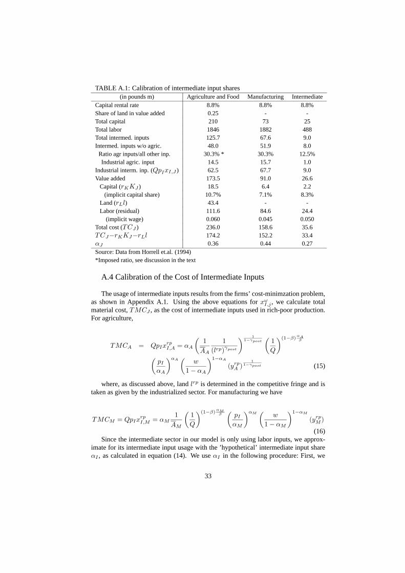
TABLE A.1: Calibration of intermediate input shares(in pounds m) Agriculture and Food Manufacturing Intermediate

Capital rental rate 8.8% 8.8% 8.8%Share of land in value added 0.25 - -Total capital 210 73 25Total labor 1846 1882 488Total intermed. inputs 125.7 67.6 9.0Intermed. inputs w/o agric. 48.0 51.9 8.0Ratio agr inputs/all other inp. 30.3% * 30.3% 12.5%Industrial agric. input 14.5 15.7 1.0

Industrial interm. inp. (QpIxI,J ) 62.5 67.7 9.0Value added 173.5 91.0 26.6

Capital (rKKJ ) 18.5 6.4 2.2(implicit capital share) 10.7% 7.1% 8.3%

Land (rLl) 43.4 - -Labor (residual) 111.6 84.6 24.4

(implicit wage) 0.060 0.045 0.050Total cost (TCJ ) 236.0 158.6 35.6TCJ−rKKJ−rLl 174.2 152.2 33.4αJ 0.36 0.44 0.27Source: Data from Horrell et.al. (1994)*Imposed ratio, see discussion in the text

A.4 Calibration of the Cost of Intermediate Inputs

The usage of intermediate inputs results from the firms’ cost-minimzation problem,as shown in Appendix A.1. Using the above equations for xωI,j , we calculate totalmaterial cost, TMCJ , as the cost of intermediate inputs used in rich-poor production.For agriculture,

TMCA = QpIxrpI,A = αA

µ1

AA

1

(lrp)γpost

¶ 11−γpost

µ1

Q

¶(1−β)αAβµpIαA

¶αA µ w

1− αA

¶1−αA(yrpA )

11−γpost (15)

where, as discussed above, land lrp is determined in the competitive fringe and istaken as given by the industrialized sector. For manufacturing we have

TMCM = QpIxrpI,M = αM

1

AM

µ1

Q

¶(1−β)αMβ µpIαM

¶αM µ w

1− αM

¶1−αM(yrpM )

(16)Since the intermediate sector in our model is only using labor inputs, we approx-

imate for its intermediate input usage with the ’hypothetical’ intermediate input shareαI , as calculated in equation (14). We use αI in the following procedure: First, we

33

calculate the total demand for each intermediate product, yI , at the point in time wherethe industrial revolution starts, i.e., in 1780.30 Second, we calculate the (hypothetical)total material cost in the intermediate sector as the share αI of total cost, that is,

TMCI = αIw

AI

yI (17)

A.5. Relative Probabilities of a kick-offIn order to find relative probabilites, we use the income figures from Maddison in

our model. That is, we update the pre-industrial productivity in each year such thatincome growth reflects the actual data. With this adjusted productivity we calculate theprobabilities of a kick-off over a range of 100 years for each country, starting in 1760.In order to reflect the hypothetical situation "What if England had not industrializedin 1780", we down-scale the Maddison income figures for England after 1780. [Thewriting of this section is in progress]

30Note that since cp > 1 at this point in time (as we explained in the calibration of pre-industrial agri-cultural productivity), there are already some industrialized manufacturing firms demanding intermediateproducts.

34

References[1] Ben-Shachar, Ari (1984). "Demand versus Supply in the Industrial Revolution: A

Comment", Journal of Economic History 44(3): 801-05.

[2] Boyer, George (1990). An Economic History of the English Poor Law, 1750-1850. Cambridge: Cambridge University Press.

[3] Broadberry, Stephen and Bishnupriya Gupta (2005). "The Early Modern GreatDivergence: Wages, Prices and Economic Development in Europe and Asia,1500-1800, Warwick working paper.

[4] CIA (2005). CIA fact book 2005: http://www.cia.gov/cia/publications/factbook/

[5] Crafts, N.F.R. (1977). "Industrial Revolution in England and France: SomeThoughts on the Question, "Why Was England First?"" Economic History Re-view, Second Series 30(3): 429-41.

[6] Crafts, N.F.R. (1995). "Exogenous or Endogenous Growth? The Industrial Revo-lution Reconsidered." Journal of Economic History 55(4): 745-72.

[7] Crafts, N.F.R. (2004a). "The First Industrial Revolution: Resolving the SlowGrowth/Rapid Industrialization Paradox". Working paper. London School of Eco-nomics

[8] Crafts, N.F.R. (1985). British Economic Growth During the Industrial Revolution.Oxford, Oxford University Press.

[9] Crafts, N.F.R. and Knick Harley (1992). ’Output Growth and the British Indus-trial Revolution: A Restatement of the Crafts-Harley View’, Economic HistoryReview, 45.

[10] Crafts, NFR (2004b), ’Steam as a General Purpose Technology: A Growth Ac-counting Perspective’, Economic Journal 114: 338-351.

[11] Crouzet, François (1965). "Capital Formation in Great Britain During the Indus-trial Revolution," in The Proceedings of the Second International; Conference ofEconomic History, The Hague. Reprinted in François Crouzet, Capital Forma-tion in the Industrial Revolution, ed. (London: Methuen & Co., Ltd., 1972). Pp.162-222.

[12] Da Rin, Marco and Thomas Hellmann (2002). "Banks as Catalysts for Industrial-ization". Journal of Financial Intermediation 11: 366-397.

[13] Feinstein, Charles H. (1988). “The Rise and Fall of the Williamson Curve”, Jour-nal of Economic History 48, pp. 699-729

[14] Feinstein, Charles H., (1998). ’Wage-earnings in Great Britain during the Indus-trial Revolution’, in I. Begg, Applied Economics and Public Policy (Cambridge1998)

35

[15] Feinstein, Charles H. (1998). ’Pessimism Perpetuated. Real Wages and the Stan-dard of Living in Britain during and after the Industrial Revolution’, Journal ofEconomic History 58.

[16] Feinstein, Charles H. and Sydney Pollard (1988): Studies in Capital Formation inthe United Kingdom 1750-1920" Clarendon Press, Oxford.

[17] Floud, R. and Johnson, P. (eds.) (2003) ’Living Standards and Urban Disameni-ties’, in: Cambridge Economic History of Britain, Cambridge: Cambridge Uni-versity Press.

[18] Foellmi, Reto and Josef Zweimüller (2004). "Inequality, Market Power, and Prod-uct Diversity." Economics Letters 82(1): 139-45.

[19] Fogel, Robert W (1984). Nutrition and the Decline in Mortality since 1700: SomePreliminary Findings, NBER Working Paper: 1402.

[20] Fogel, Robert W. (1993) ’New Sources and New Techniques for the Study of Sec-ular Trends in Nutritional Status, Mortality, and the Process of Aging’, HistoricalMethods 26.

[21] Gilboy, Elisabeth (1932), "Demand as a Factor in the Industrial Revolution", in:A.H. Cole, ed., Facts and Factors in Economic History. Cambridge, MA, HarvardUniversity Press.

[22] Galor, Oded and Omer Moav (2002). "Natural Selection and the Origin of Eco-nomic Growth." Quarterly Journal of Economics 117(4): 1133-91.

[23] Hansen, Gary D. and Edward Prescott (2002). "Malthus to Solow." AmericanEconomic Review 92(4): 1205-1217.

[24] Horrell, Sara (1996). "Home Demand and British Industrialization." Journal ofEconomic History 56(3): 561-604.

[25] Jones, Charles I (2001). "Was an Industrial Revolution Inevitable? EconomicGrowth over the Very Long Run." Advances in Macroeconomics 1(2): na.

[26] Koehn, Nancy (1995) "Josiah Wedgwood and the First Industrial Revolution",in: Thomas McCraw, Creating Modern Capitalism, Cambridge, MA: HarvardUniversity Press.

[27] Kramer, Michael (1993). "Population Growth and Technological Change: OneMillion B.C. To 1990." The Quarterly Journal of Economics 108(3): 681-716.

[28] Landes, David (1994). "No Room for Accident in History? Explaining BigChanges by Small Events." Economic History Review 48(3): 591-601.

[29] Lindert, Peter H (2000). "When Did Inequality Rise in Britain and America?"Journal of Income Distribution 9(1): 11-25.

36

[30] Lindert, Peter H and Jeffrey G Williamson (1982). "Revising England’s SocialTables, 1688-1812." Explorations in Economic History 19(4): 385-408.

[31] Lewis, Arthur (1954). "Economic Development with Unlimited Supplies ofLabour." Manchester School 22 (May 1954): 139-91.

[32] Lucas, Robert (2002). " Lectures on Economic Growth. Cambridge, MA, HarvardUniversity Press: 109-88.

[33] Maddison, Angus (2001). The World Economy : Historical Statistics. Paris,France, Development Centre of the Organisation for Economic Co-operation andDevelopment.

[34] Mankiw, Greg, Reis, Ricardo, and Justin Wolfers (2003), ’Disagreement aboutInflation Expectations’, NBER Macro Annual 18.

[35] Mokyr, Joel (1977). "Demand vs. Supply in the Industrial Revolution" Journal ofEconomic History 37(4): 981-1008.

[36] Mokyr, Joel (1999). Editor’s Introduction. The British Industrial Revolution. AnEconomic Perspective. J. Mokyr. Boulder, CA, Westview: 1-127.

[37] Murphy, Kevin M, Andrei Shleifer and Robert W Vishny (1989a). "Income Dis-tribution, Market Size, and Industrialization." Quarterly Journal of Economics104(3): 537-64.

[38] Murphy, Kevin M., Andrei Shleifer and Robert Vishny (1989b). "Industrializationand the Big Push." Journal of Political Economy 97(5): 1003-26.

[39] Pomeranz, Kenneth (2000). The Great Divergence : China, Europe, and the Mak-ing of the Modern World Economy. Princeton, N.J., Princeton University Press.

[40] Rebelo S. (1991) "Long-Run Policy Analysis and Long-Run Growth" Journal ofPolitical Economy 99, pp. 500-521.

[41] Romer, Paul M, 1990. "Endogenous Technological Change," Journal of PoliticalEconomy 98(5), pp. S71-10.

[42] Rostow, W. W. (1978). "No Random Walk: A Comment on "Why Was EnglandFirst?"" Economic History Review 31(4).

[43] Stokey, Nancy (2001). "A Quantitative Model of the British Industrial Revolution,1780-1850." Carnegie-Rochester Conference Series on Public Policy 55: 55-109.

[44] v. Tunzelmann, G.N. (1978). "Steam Power and British Industrialization to 1860",Oxford University Press

[45] Voth, Hans-Joachim (2003). "Living Standards During the Industrial Revolution:An Economist’s Guide." American Economic Review 93(2): 221-226.

[46] Williamson, Jeff (1985). ’Did British Capitalism breed Inequality?’ Boston 1985.

37

[47] Wrigley, Edward Anthony (1983). "The Growth of Population in Eighteenth-Century England: A Conundrum Resolved." Past and Present 98: 121-50.

[48] Wrigley, Edward Anthony, R.S. Davies, Jim Oeppen and Richard Schofield(1997). English Population History from Family Reconstitution 1580-1837. Cam-bridge, Cambridge University Press.

[49] Wrigley, Edward Anthony and Richard Schofield (1981). The Population Historyof England, 1541-1871: A Reconstruction. Cambridge, MA, Harvard UniversityPress.

[50] Zweimüller, Josef (2000). "Schumpeterian Entrepreneurs Meet Engel’s Law: TheImpact of Inequality on Innovation-Driven Growth." Journal of Economic Growth5(2): 185-206.

38