Why Does Deep Learning Work?

Aaron Mishkin

UBC MLRG 2019W1

1/35

Why Does Deep Learning Work?

Common refrains from deep learning:

• “Always make your neural network as big as possible!”

• “Neural networks generalize because they’re trained withstochastic gradient descent (SGD).”

• “Sharp minima are bad and shallow minima are good.”

• “SGD finds flat local minima.”

Where do these ideas come from?

2/35

Deep Learning Works!

3/35

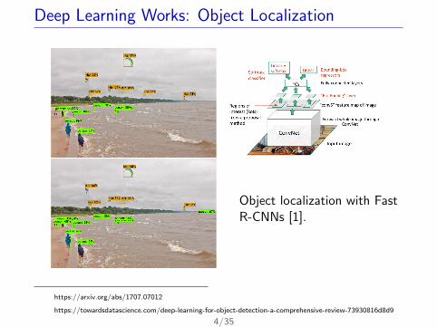
Deep Learning Works: Object Localization

https://arxiv.org/abs/1707.07012

https://towardsdatascience.com/deep-learning-for-object-detection-a-comprehensive-review-73930816d8d9

4/35

Object localization with FastR-CNNs [1].

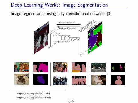
Deep Learning Works: Image Segmentation

Image segmentation using fully convolutional networks [3].

96

384

256 40

964096 21

21

backward/learning

forward/inference

pixe

lwise

pre

dict

ion

segm

enta

tion

g.t.

256

384

https://arxiv.org/abs/1411.4038

https://arxiv.org/abs/1802.02611

5/35

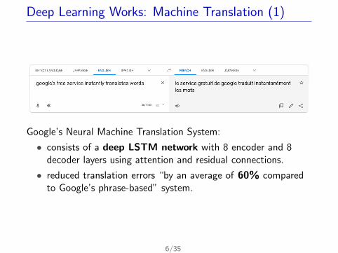
Deep Learning Works: Machine Translation (1)

Google’s Neural Machine Translation System:

• consists of a deep LSTM network with 8 encoder and 8decoder layers using attention and residual connections.

• reduced translation errors “by an average of 60% comparedto Google’s phrase-based” system.

6/35

Deep Learning Works: Machine Translation (2)

Berlin POLIZEI BERLIN The

Berlin police informs about bur-

glary protection On Thursday,

23rd May 2019, between 3:00

pm and 6:00 pm, police officers

hold an information event on bur-

glary protection in their residen-

tial area. In the process, the po-

lice will visit residential buildings

and shops and inform you directly

about security options. At the

same time, police officers at an

information stand in the Hagel-

berger Str. 34, 10965 Berlin show

them, with the help of window

and door models, how they can

effectively secure their property...

7/35

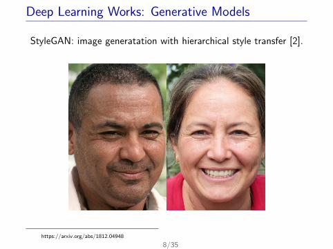
Deep Learning Works: Generative Models

StyleGAN: image generatation with hierarchical style transfer [2].

https://arxiv.org/abs/1812.04948

8/35

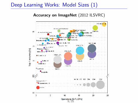
Deep Learning Works: Model Sizes (1)

Accuracy on ImageNet (2012 ILSVRC)

https://arxiv.org/abs/1810.00736

9/35

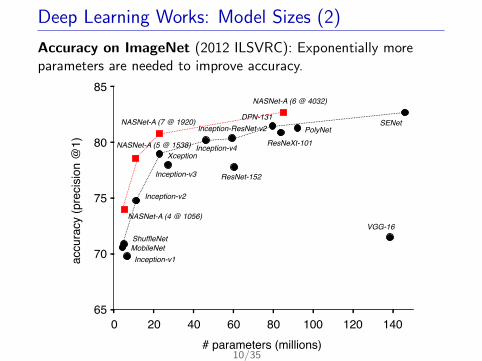
Deep Learning Works: Model Sizes (2)

Accuracy on ImageNet (2012 ILSVRC): Exponentially moreparameters are needed to improve accuracy.

75

70

65

80

85

# parameters (millions)

accu

racy

(pre

cisi

on @

1)

60 80 100 120 1400 4020

NASNet-A (5 @ 1538)

NASNet-A (4 @ 1056)VGG-16

PolyNet

MobileNetInception-v1

ResNeXt-101

Inception-v2

Inception-v4

Inception-ResNet-v2

ResNet-152

Xception

Inception-v3

ShuffleNet

DPN-131

NASNet-A (6 @ 4032)

NASNet-A (7 @ 1920) SENet

https://arxiv.org/abs/1707.07012

10/35

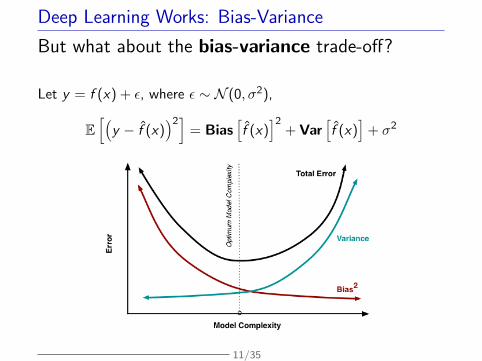
Deep Learning Works: Bias-Variance

But what about the bias-variance trade-off?

Let y = f (x) + ε, where ε ∼ N (0, σ2),

E[Ä

y − f (x)ä2]

= Biasîf (x)ó2

+ Varîf (x)ó

+ σ2

http://scott.fortmann-roe.com/docs/BiasVariance.html11/35

Bias-Variance: Deep Models

We expect bigger architectures to:

• have lower bias because have they more parameters,

• but higher variance across different training sets.

75

70

65

80

85

# parameters (millions)

accu

racy

(pre

cisi

on @

1)

60 80 100 120 1400 4020

NASNet-A (5 @ 1538)

NASNet-A (4 @ 1056)VGG-16

PolyNet

MobileNetInception-v1

ResNeXt-101

Inception-v2

Inception-v4

Inception-ResNet-v2

ResNet-152

Xception

Inception-v3

ShuffleNet

DPN-131

NASNet-A (6 @ 4032)

NASNet-A (7 @ 1920) SENet

Shouldn’t wesee this in

action withdeep models?

https://arxiv.org/abs/1707.07012

12/35

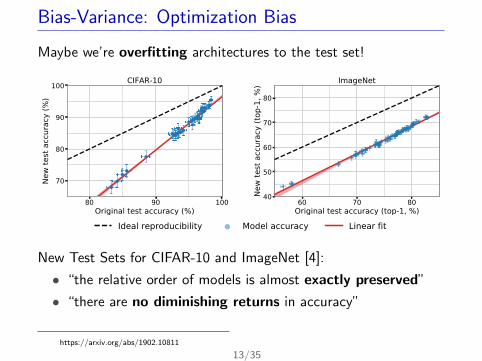
Bias-Variance: Optimization Bias

Maybe we’re overfitting architectures to the test set!

80 90 100Original test accuracy (%)

70

80

90

100

New

test

acc

urac

y (%

)

CIFAR-10

60 70 80OriginaO test accuracy (top-1, %)

40

50

60

70

80

1ew

test

acc

urac

y (t

op-1

, %) ,mage1et

Ideal reproducibility Model accuracy Linear fit

New Test Sets for CIFAR-10 and ImageNet [4]:

• “the relative order of models is almost exactly preserved”

• “there are no diminishing returns in accuracy”

https://arxiv.org/abs/1902.10811

13/35

Bias-Variance: What’s Happening?

Why do bigger neural networks leadto better accurracy?

The issue is how we think aboutmodel “capacity”.

14/35

Perceptron: An Instructive Example

15/35

Learning Theory: A Brief Introduction

Statistical learning theory tries to develop guarantees for theperformance of machine learning models.

• Let D = {(xi , yi )}ni=1 be a training set of input-output pairs.I D is formed by sampling (x , y) ∼ p(x , y) n times.

• Let H be a hypothesis class.I H is a fixed set of prediction functions f (x) = y that we

pre-select.I H could be SVMs with RBF kernels, one-layer neural networks,

etc.

• A learning algorithm takes D as input and returns f ∈ H.

What does it mean to generalize in this framework?

16/35

Learning Theory: Risk and ERM

Let L be a loss function. We care about the risk,

R(f ) = Ep(x ,y) [L(f (x), y)] .

We don’t know p(x , y), but we do have the training set D. Theempirical risk is simply the loss on D,

RD(f ) =1

n

n∑i=1

L(f (xi ), yi ).

Empirical risk minimization (ERM) is the learning algorithm

f = minf ∈H

RD(f ) = minf ∈H

1

n

n∑i=1

L(f (xi ), yi ).

This is simple – choose f to minimize the training loss.

17/35

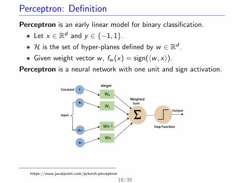
Perceptron: Definition

Perceptron is an early linear model for binary classification.

• Let x ∈ Rd and y ∈ {−1, 1}.• H is the set of hyper-planes defined by w ∈ Rd .

• Given weight vector w , fw (x) = sign(〈w , x〉).

Perceptron is a neural network with one unit and sign activation.

https://www.javatpoint.com/pytorch-perceptron

18/35

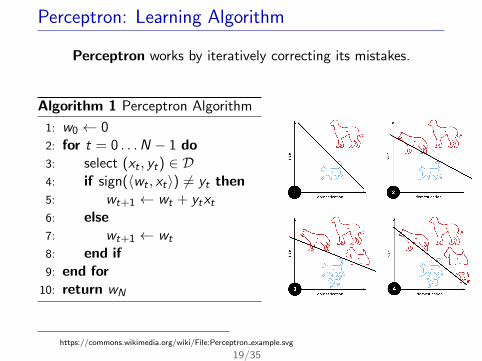
Perceptron: Learning Algorithm

Perceptron works by iteratively correcting its mistakes.

Algorithm 1 Perceptron Algorithm

1: w0 ← 02: for t = 0 . . .N − 1 do3: select (xt , yt) ∈ D4: if sign(〈wt , xt〉) 6= yt then5: wt+1 ← wt + ytxt6: else7: wt+1 ← wt

8: end if9: end for

10: return wN

https://commons.wikimedia.org/wiki/File:Perceptron example.svg

19/35

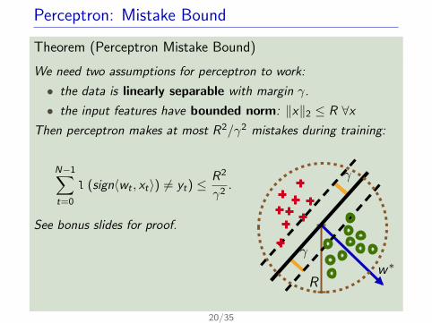
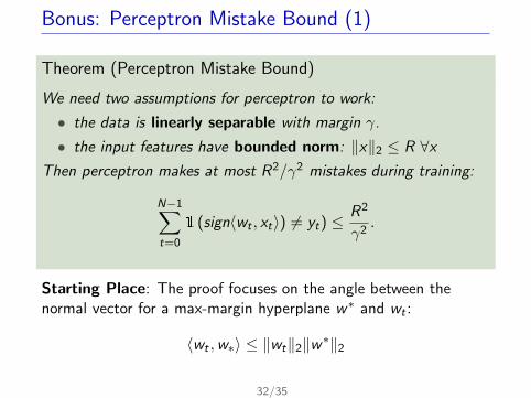
Perceptron: Mistake Bound

Theorem (Perceptron Mistake Bound)

We need two assumptions for perceptron to work:

• the data is linearly separable with margin γ.

• the input features have bounded norm: ‖x‖2 ≤ R ∀xThen perceptron makes at most R2/γ2 mistakes during training:

N−1∑t=0

1 (sign〈wt , xt〉) 6= yt) ≤R2

γ2.

See bonus slides for proof.

γ

w∗

γ

R

20/35

Perceptron: First Risk Bound

Consider doing one pass through the data to get {w0, . . . ,wn−1}.

The expected risk if we use w ′ ∼ Uniform ({w0, . . . ,wn−1}) is

R(fw ′) = Ep(x ,y)EDEt [1(sign(〈wt , x〉) 6= y)] .

Renaming (x , y) to be (xt , yt),

R(fw ′) = EDEt [1(sign(〈wt , xt〉) 6= yt)]

= ED

[1

n

n−1∑t=0

1(sign(〈wt , xt〉) 6= yt)

]This is the number of mistakes perceptron makes during training!

≤ EDï

1

n

R2

γ2

ò(by the mistake bound)

=1

n

R2

γ2

21/35

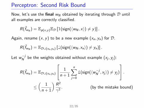
Perceptron: Second Risk Bound

Now, let’s use the final wN obtained by iterating through D untilall examples are correctly classified.

R(fwN) = Ep(x ,y)ED [1(sign(〈wN , x〉) 6= y)] .

Again, rename (x , y) to be a new example (xn, yn) for D.

R(fwN) = ED∪(xn,yn) [1(sign(〈wN , xn〉) 6= yn)] .

Let w−jN be the weights obtained without example (xj , yj):

R(fwN) = ED∪(xn,yn)

1

n + 1

n∑j=0

1(sign(〈w−jN , xj〉) 6= yj)

.≤Å

1

n + 1

ãR2

γ2. (by the mistake bound)

22/35

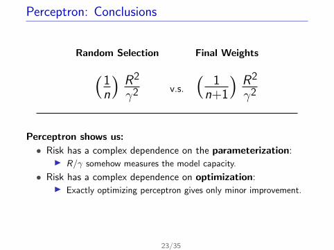
Perceptron: Conclusions

Random Selection Final Weights(1n

)R2

γ2 v.s.

(1

n+1

)R2

γ2

Perceptron shows us:

• Risk has a complex dependence on the parameterization:I R/γ somehow measures the model capacity.

• Risk has a complex dependence on optimization:I Exactly optimizing perceptron gives only minor improvement.

23/35

Why Does Deep Learning Work?

24/35

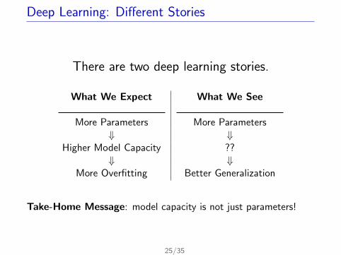
Deep Learning: Different Stories

There are two deep learning stories.

What We Expect What We See

More Parameters More Parameters⇓ ⇓

Higher Model Capacity ??⇓ ⇓

More Overfitting Better Generalization

Take-Home Message: model capacity is not just parameters!

25/35

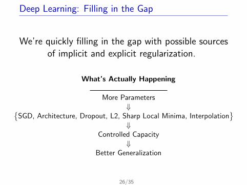
Deep Learning: Filling in the Gap

We’re quickly filling in the gap with possible sourcesof implicit and explicit regularization.

What’s Actually Happening

More Parameters⇓{

SGD, Architecture, Dropout, L2, Sharp Local Minima, Interpolation}

⇓Controlled Capacity

⇓Better Generalization

26/35

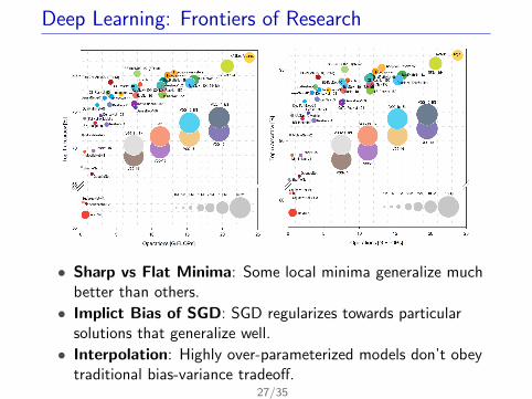
Deep Learning: Frontiers of Research

• Sharp vs Flat Minima: Some local minima generalize muchbetter than others.

• Implict Bias of SGD: SGD regularizes towards particularsolutions that generalize well.

• Interpolation: Highly over-parameterized models don’t obeytraditional bias-variance tradeoff.

27/35

Summary

Here’s what we discussed today:

• Deep neural networks work very well for a variety ofproblems.

• Making neural networks bigger improves performance evenwhen training accuracy has saturated.

• Number of parameters may be a poor measure of capacity.• New research looks at the capacity of neural networks via

I types of local minima,I properties of optimization procedures,I the role of over-parameterization/interpolation.

28/35

Signup

Signup Sheet

29/35

Acknowledgements

• The perceptron example and analysis comes from SashaRakhlin and Peter Bartlett.I See their excellent series on generalization from the

Simons Institute.

30/35

Bonus Slides

31/35

Bonus: Perceptron Mistake Bound (1)

Theorem (Perceptron Mistake Bound)

We need two assumptions for perceptron to work:

• the data is linearly separable with margin γ.

• the input features have bounded norm: ‖x‖2 ≤ R ∀xThen perceptron makes at most R2/γ2 mistakes during training:

N−1∑t=0

1 (sign〈wt , xt〉) 6= yt) ≤R2

γ2.

Starting Place: The proof focuses on the angle between thenormal vector for a max-margin hyperplane w∗ and wt :

〈wt ,w∗〉 ≤ ‖wt‖2‖w∗‖2

32/35

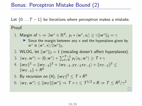
Bonus: Perceptron Mistake Bound (2)

Let {0 . . .T − 1} be iterations where perceptron makes a mistake.

Proof.

1. Margin of γ ⇒ ∃w∗ ∈ Rd , yi ∗ 〈w∗, xi 〉 ≥ γ‖w∗‖2 = γI Since the margin between any x and the hyperplane given by

w∗ is 〈w∗, x〉/‖w∗‖2.

2. WLOG, let ‖w∗‖2 = 1 (rescaling doesn’t affect hyperplanes).

3. 〈wT ,w∗〉 = 〈0,w∗〉+

∑T−1t=0 yt〈xt ,w∗〉 ≥ T ∗ γ

4. ‖wT‖2 = ‖wT−1‖2 + 〈wT−1, yT−1xT−1〉+ ‖xT−1‖2 ≤‖wT−1‖+ R2

5. By recursion on (4), ‖wT‖2 ≤ T ∗ R2

6. 〈wT ,w∗〉 ≤ ‖wT‖‖w∗‖ ⇒ T ∗ γ ≤ T 1/2 ∗ R ⇒ T ≤ R2/γ2

33/35

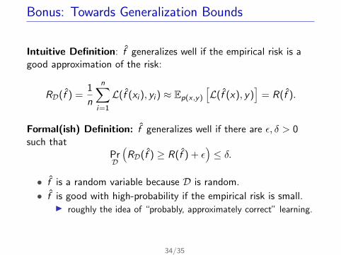
Bonus: Towards Generalization Bounds

Intuitive Definition: f generalizes well if the empirical risk is agood approximation of the risk:

RD(f ) =1

n

n∑i=1

L(f (xi ), yi ) ≈ Ep(x ,y)

îL(f (x), y)

ó= R(f ).

Formal(ish) Definition: f generalizes well if there are ε, δ > 0such that

PrD

ÄRD(f ) ≥ R(f ) + ε

ä≤ δ.

• f is a random variable because D is random.

• f is good with high-probability if the empirical risk is small.I roughly the idea of “probably, approximately correct” learning.

34/35

References I

Ross Girshick.Fast r-cnn object detection with caffe.Microsoft Research, 2015.

Tero Karras, Samuli Laine, and Timo Aila.A style-based generator architecture for generative adversarial networks.In Proceedings of the IEEE Conference on Computer Vision and PatternRecognition, pages 4401–4410, 2019.

Jonathan Long, Evan Shelhamer, and Trevor Darrell.Fully convolutional networks for semantic segmentation.In Proceedings of the IEEE conference on computer vision and patternrecognition, pages 3431–3440, 2015.

Benjamin Recht, Rebecca Roelofs, Ludwig Schmidt, and VaishaalShankar.Do imagenet classifiers generalize to imagenet?arXiv preprint arXiv:1902.10811, 2019.

35/35