DI

SC

US

SI

ON

P

AP

ER

S

ER

IE

S

Forschungsinstitut zur Zukunft der ArbeitInstitute for the Study of Labor

Why Do Some Motorbike Riders Wear a Helmet and Others Don‘t? Evidence from Delhi, India

IZA DP No. 8042

March 2014

Michael GrimmCarole Treibich

Why Do Some Motorbike Riders

Wear a Helmet and Others Don’t? Evidence from Delhi, India

Michael Grimm Erasmus University Rotterdam,

Passau University and IZA

Carole Treibich Paris School of Economics, Erasmus University Rotterdam

and Aix-Marseille University, CNRS & EHESS

Discussion Paper No. 8042 March 2014

IZA

P.O. Box 7240 53072 Bonn

Germany

Phone: +49-228-3894-0 Fax: +49-228-3894-180

E-mail: iza@iza.org

Any opinions expressed here are those of the author(s) and not those of IZA. Research published in this series may include views on policy, but the institute itself takes no institutional policy positions. The IZA research network is committed to the IZA Guiding Principles of Research Integrity. The Institute for the Study of Labor (IZA) in Bonn is a local and virtual international research center and a place of communication between science, politics and business. IZA is an independent nonprofit organization supported by Deutsche Post Foundation. The center is associated with the University of Bonn and offers a stimulating research environment through its international network, workshops and conferences, data service, project support, research visits and doctoral program. IZA engages in (i) original and internationally competitive research in all fields of labor economics, (ii) development of policy concepts, and (iii) dissemination of research results and concepts to the interested public. IZA Discussion Papers often represent preliminary work and are circulated to encourage discussion. Citation of such a paper should account for its provisional character. A revised version may be available directly from the author.

IZA Discussion Paper No. 8042 March 2014

ABSTRACT

Why Do Some Motorbike Riders Wear a Helmet and Others Don’t? Evidence from Delhi, India

We focus on helmet use behavior among motorbike users in Delhi. We use a detailed data set collected for the purpose of the study. To guide our empirical analysis, we rely on a simple model in which drivers decide on self-protection and self-insurance. The empirical findings suggest that risk averse drivers are more likely to wear a helmet, there is no systematic effect on speed. Helmet use also increases with education. Drivers who show a higher awareness of road risks are both more likely to wear a helmet and to speed less. Controlling for risk awareness, we observe that drivers tend to compensate between speed and helmet use. The results can provide a basis for awareness-raising policies. Improvements to the road infrastructure bear the risk of leading to risk-compensating behavior. JEL Classification: D10, I10, I15, K42, R41 Keywords: road safety, helmet use, risky health behavior, self-protection, self-insurance,

India Corresponding author: Michael Grimm University of Passau Innstrasse 29 94032 Passau Germany E-mail: michael.grimm@uni-passau.de

In some states of India, women are exempted from safety rules that mandate motorcycle passengers wear

helmets – an exemption that kills or injures thousands each year. Women’s rights advocates have argued the

exemption springs from a culture-wide devaluation of women’s lives. Supporters of the ban say they’re just

trying to preserve women’s carefully styled hair and make-up – which isn’t exactly a feminist response.

(Washington Post, October 27, 2013)

1 Introduction

Nearly 3,500 people die on the world’s roads every day. 90% of these fatalities occur in

developing countries (WHO, 2009). In 2020, road traffic injuries are expected to be ranked

third in the global burden of disease (Lopez et al., 2006). Despite these numbers and the

related tremendous costs, road mortality is still a neglected public health issue in many

low and middle income countries. India accounts for about 10% of road accident fatalities

worldwide. The implied costs are estimated at around 3% of GDP (Mohan, 2002). In many

developing countries, the share of two-wheeled vehicles largely dominates the vehicle fleet. In

India this share is around 70%. Not surprisingly motorbike users constitute a large share of

all road traffic accident injuries and fatalities; in Delhi for instance more than 30%. Injuries

to the head and the neck are the main cause of death, indeed 60% of All India Institute

of Medical Sciences’ (AIIMS) admissions — one of the biggest trauma centers in Delhi —

are road related head injuries (see also Kumar et al., 2008). Medical science stresses the

efficiency of helmets in reducing the road related mortality and morbidity. Mandatory helmet

use is thus one important policy that governments are recommended to implement in order to

reduce road-related fatalities (WHO, 2004, 2006). The effectiveness of such laws, if enforced,

has been shown in various contexts (see, e.g., Dee, 2009; French et al., 2009). Despite the

formal introduction of such laws in most countries of the world (WHO, 2009), enforcement

is however often very weak. Moreover motorbike users are often not aware of the protection

that a helmet can provide.

India has had a helmet law since 1988. This national law should be implemented at the

State level, yet it is hardly enforced. A major complication comes from the fact that the Sikh

community successfully lobbied against this law as their religion requires a turban or at least

no other headpiece. Since the exception also applies to Sikh women, and hence it is difficult

to distinguish Sikh from other women, the exception was later extended to all women. In

2

Delhi less than 25% of all women wear a helmet when sitting on a motorbike — typically in

the poised perched side-saddle position.1 For men the share of helmet wearers is significantly

higher, but is still far from full coverage. Understanding this heterogeneity, i.e. why some

drivers and passengers wear a helmet and others not, is key to design effective interventions

to increase helmet use.

Helmet use might be linked to risk aversion, the awareness of road-related risks, income,

and as seen above, culture and traditions. Moreover, motorbike riders have various options to

protect themselves or to seek insurance. Speed is obviously a second important decision pa-

rameter. To understand the behavior of helmet use, we first model this problem theoretically.

Relying on the literature of self-insurance and self-protection, we develop a simple model that

can be used for comparative static analysis. Based on this analysis we derive hypotheses

which we test empirically using a unique data set covering more than 850 motorbike riders

and passengers in Delhi.2

The remainder of the paper is organized as follows. In section 2 we briefly review the

related literature, highlight the existing knowledge gaps and elaborate on the paper’s contri-

bution. Section 3 presents the theoretical framework and derives from it testable predictions

regarding helmet use and speed. Section 4 introduces the data set. Section 5 shows how we

operationalize the empirical tests. Section 6 presents the empirical analysis and discusses the

results. Section 7 concludes.

2 Related literature

In what follows we briefly review the theoretical literature that considers the role of risk

aversion on individual investment in different accident prevention activities. We emphasize

in particular the role of risk compensating effects. After that we discuss the related empirical

evidence.

Both Peltzman (1975) and Blomquist (1986) modeled the driver’s behavior and derived

insightful predictions for risk neutral agents. They focused in particular on risk compensation

effects, i.e. behavioral responses to exogenous variations in risk. Others enriched such mod-

els with explicit consideration of the risk preferences of agents in their behavioral response.

1Figures derived from a household survey implemented by the authors in Delhi. See below.2This paper builds on Grimm and Treibich (2013) in which we study the determinants of road traffic

accident fatalities across Indian states over time.

3

Dionne and Eeckhoudt (1985) and Bryis and Schlesinger (1990), for example, examined the-

oretically the impact of increased risk aversion on the optimal levels of self-insurance and

self-protection. Self-insurance refers to activities that reduce the severity of a loss. Self-

protection decreases the probability that the loss occurs (Ehrlich and Becker, 1972). In their

models the level of self-insurance monotonically increases with risk aversion, while the effect

of risk aversion is ambiguous regarding self-protection. In other words, a more risk averse in-

dividual will always invest more in self-insurance but it is possible that the individual chooses

a lower level of self-protection. Indeed, self-protection reduces the occurrence of a loss but

does not reduce the loss in case the bad state occurs. Rather to the contrary, in addition to

the loss, wealth is reduced by the increased cost of self-protection, thus leading to an even

worse outcome if the bad state occurs. Hence, a higher level of self-protection might be con-

sidered as more, not less risky and may explain why a more risk averse individual might decide

to invest less in such an activity. Finally, when combining both activities and investigating

the influence of risk aversion on a self-insurance-cum-protection activity, a more risk averse

individual will invest more in the prevention activity, if the marginal loss reduction in the bad

state out-weights the marginal increase in the cost of the combined activity. This has been

shown by Lee (1998).

Peltzman (1975) and Wilde (1982) introduced the idea that individuals may respond to an

exogenous increase in safety in a way that it lowers or even annihilates (risk homostasis) the

reduced risk. Such reactions are called ‘risk compensation effects’ and may arise if individuals

target a fixed level of risk and therefore prefer taking more risks when their risk environment

improves. Some studies empirically tested whether such effects indeed exist. However, these

studies typically rely on highly aggregated data and hence potentially suffer from omitted

variable bias. Chirinko and Harper Jr. (1993), for example, investigated the effect of improved

car safety (measured through an index of safety regulations in relation to improved car safety

for occupants since 1966) and of the introduction of the speed limit of 55 mph in the US. Their

econometric estimates revealed that the offsetting behavior is quantitatively important and

attenuates the effects of safety regulations on occupant fatalities. Using a modified expected

utility model, the authors showed that the impact of regulatory policies depends on a mix

of protection (direct effect of the regulation), substitution (offsetting behavior) and cognition

elements. Based on Virginia State Police accident reports of 1993, Peterson et al. (1995) also

4

showed that air-bag-equipped cars tend to be driven more aggressively, thus offsetting the

effect of the air-bag for drivers and increasing the risk of death for others. However, other

studies did not find any evidence of such risk-compensating effects (Lund and Zador, 1984;

Lund and O’Neill, 1986).

To circumvent problems inherent in the use of aggregate data, Sobel and Nesbit (2007)

used micro-level data from NASCAR (National Association for Stock Car Auto Racing) races.

Their setting allowed them to control for problems of enforcement, weather conditions and

variation in automobile safety devices. According to their results, NASCAR drivers drive more

recklessly in response to an increase in car safety. However, total injuries still fall since the

side effect is not large enough to completely offset the direct impact of increased vehicle safety.

Obviously, the external validity of this study might be low, as NASCAR drivers might not be

very representative of drivers in general. Stetzer and Hofmann (1996) in turn conducted two

laboratory experiments to investigate the individual’s behavioral response and the perceived

risk associated with various driving situations. They found a negative correlation indicating

some risk compensation following an increase in environmental safety but this was not large

enough to return to the initial level of risk. Messiah et al. (2012) ran a randomized controlled

trial in Bordeaux to analyze motorcyclists’ chosen speed conditional on helmet adoption. Risk

compensation was observed exclusively among men and was of moderate size. Therefore the

feedback effect did not offset the benefits of helmet use.

McCarthy and Talley (1999) also provided evidence on risk compensating behaviors. They

relied on data from recreational boating. They empirically tested whether an operator’s past

experience and formal training induces or reduces safety related behaviors. Moreover they

investigated the influence of the operator’s characteristics and the environmental factors on

the attitude adopted by the boat passengers. The authors highlighted that an individual

can adjust to risk changes using various strategies. In their study, they focused on two of

them: the use of personal flotation devices and alcohol consumption. Passengers seemed to

adapt their behavior to their perception of the operator’s safety level. Indeed, an operator’s

boating experience was negatively correlated with flotation device utilization and positively

correlated with alcohol consumption by passengers. The authors stressed the implication for

motor vehicle travel. In particular, they pointed out that, since the opening of the debate by

Peltzman (1975), little work has been done to identify alternative margins that individuals

5

use to adjust their safety behavior.

We contribute to the above literature with respect to two dimensions: (i) the influence

of risk aversion on prevention activities and (ii) the existence of risk compensating effects.

Regarding the first aspect, we derive theoretical predictions regarding the role of risk aversion

on a set of different types of prevention efforts. Moreover, thanks to an original dataset of

motorbike riders and passengers in Delhi, we are able to test these assumptions empirically.

In particular, we focus on the drivers’ simultaneous decision-making with respect to self-

protection and self-insurance and how risk preferences affect this trade-off. With respect to

the second dimension, we look at the existence of risk compensating effects. An interesting

feature of our data is that we also observe passengers. For passengers speed can be seen as

exogenously determined if the assumption is made that the driver decides on speed. We are

thus able to investigate the relation between a passenger’s safety effort and the environment

such as the quality of roads and motorbike and driver characteristics. As for the driver, we

can examine the relationship between alternative dimensions of safety behaviors and whether

they are complements or substitutes.

3 Theoretical framework

Building on Dionne and Eeckhoudt (1985) and Bryis and Schlesinger (1990), we investigate the

individual decision to invest in self-insurance and self-protection activities using a relatively

simple expected utility model. As in Ehrlich and Becker (1972), self-insurance refers to any

activity that reduces the loss if an accident occurs, while self-protection refers to any activity

that reduces the probability of experiencing an accident.

In our theoretical framework we address three questions: (i) How does risk aversion in-

fluence the investment in insurance and protection? (ii) How do motorbike users respond to

exogenous changes in safety? (iii) Are protection and insurance complements or substitutes

for one another?

We consider two road related attitudes: helmet use and speed. Helmet use can be seen as

a self-insurance activity given that a helmet reduces the severity of an injury if an accident

6

occurs.3 For simplicity, lowering speed is assumed to be a self-protection activity.4 While we

assume that the drivers of a motorbike choose both helmet use and speed, we assume that

passengers only make a decision on helmet use, and take speed as given. We examine these

two types of road users in turn. We start with the case of passengers.

3.1 Passengers

Consider a risk averse passenger with wealth W . With a probability p, the passenger is

involved in a road accident and with probability (1− p) the passenger is not. If an accident

occurs, the passenger faces a loss I; however, the passenger can invest in the self-insurance

activity to reduce the size of the potential loss. This decision includes whether to use a helmet,

the type of helmet and whether for instance the strap is closed. However, helmet use comes

at a cost in the form of discomfort. Let h denote the level of self-insurance. I(h) represents

the effect of a helmet on the severity of an injury, which is obviously assumed to decrease

with the chosen level of self-insurance, I ′(h) < 0. Discomfort, c(h), is assumed to increase

monotonically with h. Preferences, U(·), are assumed to be of the von Neumann-Morgenstern

type, where U ′ > 0 and U ′′ < 0.

The individual’s expected utility can be written as:

EU = p · U [W − c(h)− I(h)] + (1− p) · U [W − c(h)]. (1)

The first order condition for maximizing (1) with respect to h is:

∂EU

∂h= −p · [c′(h) + I ′(h)] · U ′(B)− (1− p) · c′(h) · U ′(G) = 0, (2)

where G = W − c(h) and B = W − c(h)− I(h).

Note that in order to have an interior solution, we must have [c′(h) + I ′(h)] < 0, i.e. the

magnitude of the potential marginal benefit, −I ′(h), must be at least as high as the marginal

3Indeed Liu et al. (2008) reviewed 53 studies that investigate the efficiency of helmets. They found thaton average the use of a standardized helmet reduces the risk of death and serious injuries by 40% and 70%respectively. Goldstein (1996) stressed however that there is a ‘head-neck injury trade-off’, i.e. given theweight of a helmet, the use of a helmet increases the risk of neck injuries.

4We acknowledge that it could also be assumed that speed is rather a self insurance-cum-protection activity,since speed may impact on both the frequency and severity of road accidents. However, to ease the resolutionof the system of equations we opt for this simplification.

7

cost following the increase in h, c′(h). Indeed, the passenger will certainly not choose a level of

helmet-use for which the perceived marginal discomfort exceeds the marginal benefit. Given

the concavity of the utility function, the second-order condition for the maximization problem

can be easily derived.

3.1.1 Risk aversion

Let hU denote the optimal level of insurance for the passenger with utility function U defined

above. Let us now consider a second, more risk averse, passenger with a utility function V

which exhibits higher risk aversion than U , i.e. V (·) is a concave increasing transformation

of U(·), hence V (·) = g[U(·)], with g′ > 0, and g′′ < 0 (Pratt, 1964).

Assuming the same wealth prospect and choice set as (2) but taking into account the

preferences of the more risk averse individual, we obtain:

∂EV

∂h= −p · [c′(h) + I ′(h)] · g′(U(B)) · U ′(B)− (1− p) · c′(h) · g′(U(G)) · U ′(G). (3)

To see whether a more risk averse individual invests more in self-insurance, we need

to evaluate∂EV

∂hat h = hU . Since, g′′ < 0, we have g′(U(B)) > g′(U(G)). Therefore,

when computing∂EV

∂hat the optimal point hU (for which we have

∂EU

∂h= 0) we obtain

∂EV

∂h|h=hU

> 0. In other words, a more risk averse passenger invests more in self-insurance,

i.e. helmet use.

3.1.2 Risk compensating effect

We consider again the passenger with utility function U and explore an increase in the prob-

ability that an accident occurs from p to q, where q > p. Substituting q in Equation (2), we

obtain:∂EU(q)

∂h= −q · [c′(h) + I ′(h)] · U ′(B)− (1− q) · c′(h) · U ′(G). (4)

To see whether the passenger invests more in self-insurance following an exogenous increase

in the probability that an accident occurs, we need to evaluate∂EU(q)

∂hat h = hU . Since q > p

and −[c′(h) + I ′(h)] > 0 (the condition for an interior solution), we have −q · [c′(h) + I ′(h)] >

−p · [c′(h) + I ′(h)] and (1− q) · c′(h) < (1− p) · c′(h). Thus, when computing∂EU(q)

∂hat the

8

optimal point hU , we obtain∂EU(q)

∂h|h=hU

> 0, i.e. if the probability that an accident occurs

increases, the passenger invests more in self-insurance and hence compensate at least partially

for the increased risk. In turn, if safety increases exogenously, passengers are thought to invest

less. As explained above, in the literature, this effect is called “Peltzman-effect” (Peltzman,

1975).

3.2 Drivers

Unlike passengers, drivers are assumed to invest simultaneously in self-insurance (helmet use)

and in self-protection (speed). It is assumed that the probability that an accident occurs,

p(s), increases with speed, p′(s) > 0. The time spent on the road t(s) in turn decreases with

speed, i.e. t′(s) < 0 and thus leaves the driver with a higher level of wealth. As for passengers,

we assume that drivers are risk averse and have an increasing concave utility function U .

In this case the expected utility is given as:

EU = p(s) · U [W − t(s)− c(h)− I(h)] + (1− p(s)) · U [W − t(s)− c(h)]. (5)

The first order conditions for maximizing (5) with respect to h and s are:

∂EU

∂h= −p(s) · [c′(h) + I ′(h)] · U ′(B)− (1− p(s)) · c′(h) · U ′(G) = 0 and (6)

∂EU

∂s= p′(s) · [U(B)− U(G)]− t′(s) · [p(s) · U ′(B) + (1− p(s)) · U ′(G)] = 0. (7)

3.2.1 Risk aversion

Again we consider the case of two individuals, i.e. here drivers, with different degrees of

risk-aversion, U and V :

∂EV

∂h= −p(s) · [c′(h) + I ′(h)] · g′(U(B)) · U ′(B)− (1− p(s)) · c′(h) · g′(U(G)) · U ′(G) (8)

and

∂EV

∂s= p′(s)·[g(U(B))−g(U(G))]−t′(s)·[p(s)·g′(U(B))·U ′(B)+(1−p(s))·g′(U(G))·U ′(G)].

(9)

9

To see whether the more risk averse driver invests more in self-insurance and self-protection,

we need to compute the sign of Equations (8) and (9) at h = hU and s = sU respectively.

The results show that in such a framework a more risk averse individual invests more in

self-insurance, while the effect on self-protection is ambiguous. As explained above this is due

to the fact that a more risk averse individual invests always more in self-insurance but not

necessarily in self-protection. Indeed, self-protection reduces the occurrence of a loss but does

not reduce the loss in case the accident occurs. Rather to the contrary, in addition to the loss,

wealth is reduced by the increased cost of self-protection, leading to an even worse outcome

if the accident occurs. Hence, a higher level of self-protection can be considered as more, not

less risky and can explain why a more risk averse individual may not necessarily decide to

invest more in such an activity (Dionne and Eeckhoudt, 1985; Bryis and Schlesinger, 1990).

3.2.2 Risk compensating effect

Again, we investigate the case of an individual with the utility function U and investigate

the influence of a change in the probability that an accident takes place on helmet use by

drivers. Such variation may be exogenous (as in the case with passengers) or endogenous. An

exogenous increase in the probability of accident may occur following the deterioration of road

quality, increased traffic density or adverse weather conditions. Obviously, just as passengers

do, drivers invest more in self-insurance following an exogenous rise in the probability that an

accident occurs. In the case of drivers, it is important to note that any change in speed has

also wealth effects, as the travel time is altered. The marginal change in helmet use following

a marginal change in speed is given by the following cross-derivative:

∂2EU

∂h∂s= p′(s) · (−[c′(h) + I ′(h)] · U ′(B) + c′(h) · U ′(G))+

t′(s) · (p(s) · [c′(h) + I ′(h)] · U ′′(B) + (1− p(s)) · c′(h) · U ′′(G)). (10)

Using Equation (6), we obtain the following two equalities:

10

−[c′(h) + I ′(h)] · U ′(B) =

(1− p(s)p(s)

· c′(h) · U ′(G) and

p(s) · [c′(h) + I ′(h)] = −(1− p(s)) · c′(h) · U′(G)

U ′(B).

Replacing these two equalities in Equation (10) allows us to derive the sign of the cross

derivative at the optimal point hU :

∂2EU

∂h∂s|h=hU

=p′(s)

p(s)· c′(h) · U ′(G) + t′(s) · (1− p(s)) · c′(h) · [U ′′(G)− U ′(G)

U ′(B)· U ′′(B)]. (11)

Assuming a constant relative risk aversion rate (−U′′(G)

U ′(G)= −U

′′(B)

U ′(B)= r), we find that

∂2EU

∂h∂s|h=hU

> 0. Therefore, when a driver increases speed, he or she also increases helmet

use. In other words, for risk averse drivers, helmet use and higher speed are complements,

and hence self-insurance and self-protection activities are substitutes.

3.2.3 Awareness

There are different options to model awareness in our framework. The most obvious way is to

assume that increased awareness implies that the expected probability of an accident at any

speed and the expected gain of helmet use should an accident occur is not underestimated

relative to actual figures.

Case #1: Raising the expected probability that an accident occurs at any speed

level

We denote the initial probability p and the probability after awareness has risen qA, i.e.

qA > p. Hence, we substitute in Equations (6) and (7) p by qA and obtain:

∂EU1

∂h= −qA(s) · [c′(h) + I ′(h)] · U ′(B)− (1− qA(s)) · c′(h) · U ′(G) and (12)

∂EU1

∂s= q′A(s) · [U(B)− U(G)]− t′(s) · [qA(s) · U ′(B) + (1− qA(s)) · U ′(G)]. (13)

11

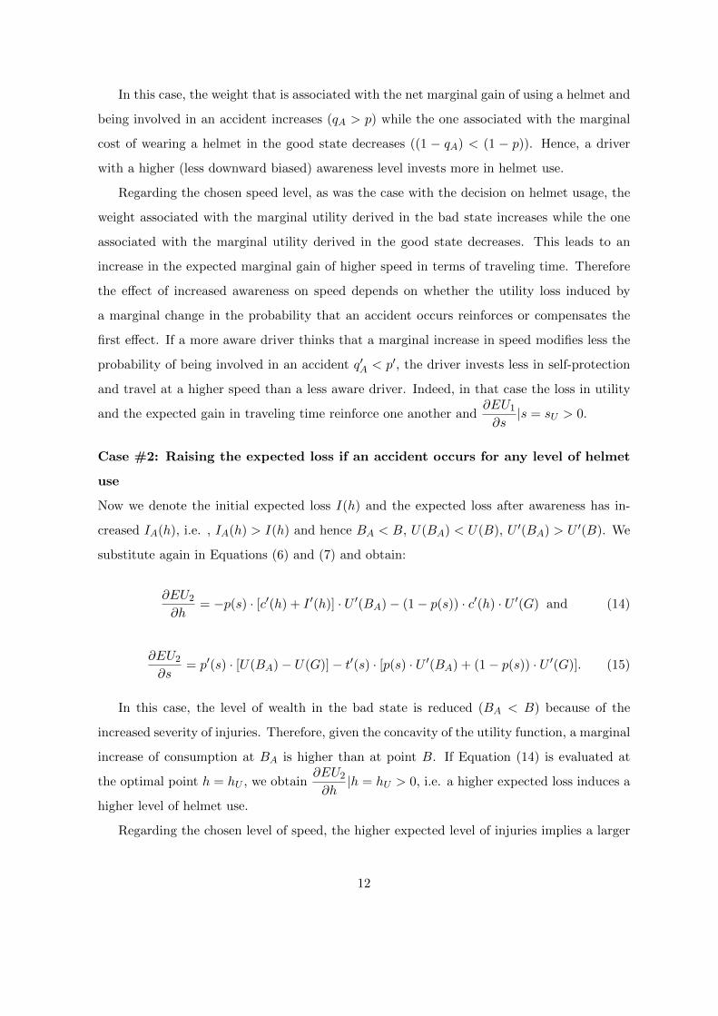
In this case, the weight that is associated with the net marginal gain of using a helmet and

being involved in an accident increases (qA > p) while the one associated with the marginal

cost of wearing a helmet in the good state decreases ((1 − qA) < (1 − p)). Hence, a driver

with a higher (less downward biased) awareness level invests more in helmet use.

Regarding the chosen speed level, as was the case with the decision on helmet usage, the

weight associated with the marginal utility derived in the bad state increases while the one

associated with the marginal utility derived in the good state decreases. This leads to an

increase in the expected marginal gain of higher speed in terms of traveling time. Therefore

the effect of increased awareness on speed depends on whether the utility loss induced by

a marginal change in the probability that an accident occurs reinforces or compensates the

first effect. If a more aware driver thinks that a marginal increase in speed modifies less the

probability of being involved in an accident q′A < p′, the driver invests less in self-protection

and travel at a higher speed than a less aware driver. Indeed, in that case the loss in utility

and the expected gain in traveling time reinforce one another and∂EU1

∂s|s = sU > 0.

Case #2: Raising the expected loss if an accident occurs for any level of helmet

use

Now we denote the initial expected loss I(h) and the expected loss after awareness has in-

creased IA(h), i.e. , IA(h) > I(h) and hence BA < B, U(BA) < U(B), U ′(BA) > U ′(B). We

substitute again in Equations (6) and (7) and obtain:

∂EU2

∂h= −p(s) · [c′(h) + I ′(h)] · U ′(BA)− (1− p(s)) · c′(h) · U ′(G) and (14)

∂EU2

∂s= p′(s) · [U(BA)− U(G)]− t′(s) · [p(s) · U ′(BA) + (1− p(s)) · U ′(G)]. (15)

In this case, the level of wealth in the bad state is reduced (BA < B) because of the

increased severity of injuries. Therefore, given the concavity of the utility function, a marginal

increase of consumption at BA is higher than at point B. If Equation (14) is evaluated at

the optimal point h = hU , we obtain∂EU2

∂h|h = hU > 0, i.e. a higher expected loss induces a

higher level of helmet use.

Regarding the chosen level of speed, the higher expected level of injuries implies a larger

12

loss in terms of wealth leading to both a greater difference in utilities between the two states

of the world (U(G) − U(BA) > U(G) − U(B)) and a higher marginal utility in the bad

state (U ′(BA) > U ′(B)). Given the former, a marginal increase in speed increases the loss.

Moreover, the marginal increase in speed also raises the level of gain in terms of travelling

time due to the latter effect. Hence, again, the effect of an increase in the expected level of

injuries on speed is ambiguous. Note that in this case the utility of helmet use remains the

same, i.e. I ′(h) is constant.

4 Data

4.1 General presentation

During the months July to September 2011 we conducted a household survey in Delhi to

collect information from motorbike riders and pillion passengers regarding their behavior when

using the motorbike including helmet use and speed, their degree of risk aversion and risk

awareness. In addition the survey collected socio-demographic and economic characteristics,

information on insurance coverage as well as characteristics of the motorbike in use. To ensure

representativeness in the survey with respect to Delhi’s population, the following sampling

design was applied: (i) Delhi was divided into five zones, (ii) in each zone, ten polling booths

were randomly drawn, (iii) the location of these polling booths were taken as starting points

from which every fifth household was selected for an interview. Around each polling booth, 30

households were interviewed. In total 1,502 households were surveyed. In 545 households at

least one member had used a motorbike in the past four weeks. These households were given a

long questionnaire. All other households only received a short questionnaire.5 In households

with at least one motorbike user, up to three, either drivers or passengers, were selected. On

average, there were two eligible members per household. 212 selected individuals refused to

answer to the questionnaire, leading to a final sample of 902 individuals which corresponds

to a response rate of 81%. Yet, among those who have answered to our survey, there are

respondents who could not or did not want to answer to some of the questions. We decided to

use in our analysis always the largest possible sample. However we show that our results across

different specifications are robust to the exact sample chosen. We also show in the appendix, a

5The short questionnaire only includes basic socio-demographic information.

13

probit model in which we regress for drivers and passengers a dummy variable “having at least

one missing variable” on a set of basic socio-demographic and socio-economic variables (Table

A1). It can be seen that for male drivers, none of these variables is significant, suggesting

that non-reporting is rather random. For passengers we see that women, higher income and

caste categories are more likely to have some missing information. All our regressions below

control for these characteristics to exclude any bias, yet there is obviously still a risk that

non-reporting is tight to relevant non-observable characteristics. Not surprisingly, income is

the variable where most of the missings occur. In our regressions below we introduce (but

do not show) next to the various income categories a category “income not reported”. This

dummy was in none of the regressions significant, also suggesting that there is no systematic

non-reporting in the data.

Moreover, given the importance of gender in our analysis, we analyze men and women

separately. Since, we do only have 15 female drivers in our sample. These are not part of a

separate analysis. We also have 27 individuals in the sample that reported to be sometimes

a driver and sometimes a passenger. They are also excluded from the driver and passenger

samples.

Given that road usage behavior, helmet use and speed vary a lot with the distance of a

trip, the type of roads used and traffic density, for each user we collected information for up

to three different types of trips: trips in the neighborhood, short distance trips (partly outside

the neighborhood) and long distance trips. Hence, in the empirical analysis we exploit the

variation across different types of trips using single trips as the unit of analysis and clustering

standard errors at the individual level.

[insert Table 1 here]

Table 1 shows some basic descriptive statistics of our sample, separated by drivers and

passengers. The average age is 35 years for drivers and 38 years for passengers. Almost all

drivers are men, passengers are predominantly female (75%). Drivers are typically married

and are the main bread winners in their household. Among male passengers 69% reported to

be married and 69% of them contribute to household income. Among female passengers the

share married is even at 86%. The education level is relatively high. Almost 50% of all drivers

completed middle or high school. The education level of passengers is significantly lower. The

14

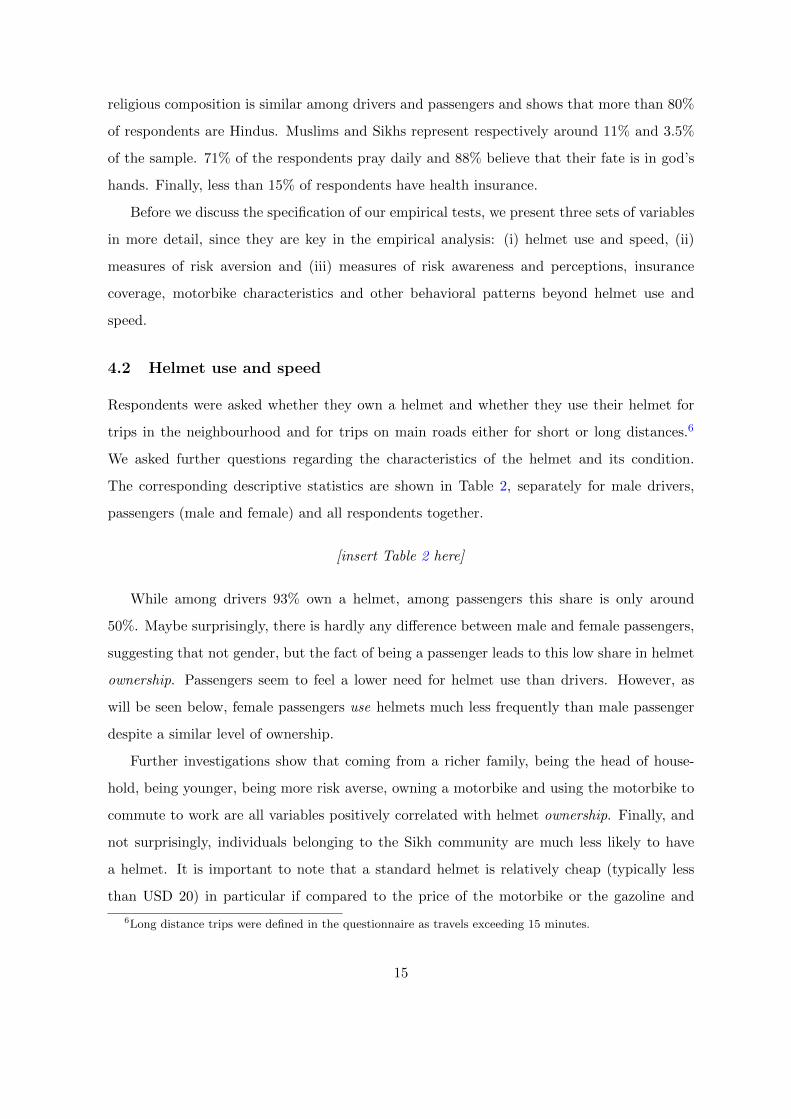
religious composition is similar among drivers and passengers and shows that more than 80%

of respondents are Hindus. Muslims and Sikhs represent respectively around 11% and 3.5%

of the sample. 71% of the respondents pray daily and 88% believe that their fate is in god’s

hands. Finally, less than 15% of respondents have health insurance.

Before we discuss the specification of our empirical tests, we present three sets of variables

in more detail, since they are key in the empirical analysis: (i) helmet use and speed, (ii)

measures of risk aversion and (iii) measures of risk awareness and perceptions, insurance

coverage, motorbike characteristics and other behavioral patterns beyond helmet use and

speed.

4.2 Helmet use and speed

Respondents were asked whether they own a helmet and whether they use their helmet for

trips in the neighbourhood and for trips on main roads either for short or long distances.6

We asked further questions regarding the characteristics of the helmet and its condition.

The corresponding descriptive statistics are shown in Table 2, separately for male drivers,

passengers (male and female) and all respondents together.

[insert Table 2 here]

While among drivers 93% own a helmet, among passengers this share is only around

50%. Maybe surprisingly, there is hardly any difference between male and female passengers,

suggesting that not gender, but the fact of being a passenger leads to this low share in helmet

ownership. Passengers seem to feel a lower need for helmet use than drivers. However, as

will be seen below, female passengers use helmets much less frequently than male passenger

despite a similar level of ownership.

Further investigations show that coming from a richer family, being the head of house-

hold, being younger, being more risk averse, owning a motorbike and using the motorbike to

commute to work are all variables positively correlated with helmet ownership. Finally, and

not surprisingly, individuals belonging to the Sikh community are much less likely to have

a helmet. It is important to note that a standard helmet is relatively cheap (typically less

than USD 20) in particular if compared to the price of the motorbike or the gazoline and

6Long distance trips were defined in the questionnaire as travels exceeding 15 minutes.

15

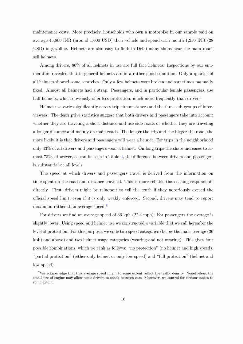
maintenance costs. More precisely, households who own a motorbike in our sample paid on

average 45,800 INR (around 1,000 USD) their vehicle and spend each month 1,250 INR (28

USD) in gazoline. Helmets are also easy to find; in Delhi many shops near the main roads

sell helmets.

Among drivers, 86% of all helmets in use are full face helmets. Inspections by our enu-

merators revealed that in general helmets are in a rather good condition. Only a quarter of

all helmets showed some scratches. Only a few helmets were broken and sometimes manually

fixed. Almost all helmets had a strap. Passengers, and in particular female passengers, use

half-helmets, which obviously offer less protection, much more frequently than drivers.

Helmet use varies significantly across trip circumstances and the three sub-groups of inter-

viewees. The descriptive statistics suggest that both drivers and passengers take into account

whether they are traveling a short distance and use side roads or whether they are traveling

a longer distance and mainly on main roads. The longer the trip and the bigger the road, the

more likely it is that drivers and passengers will wear a helmet. For trips in the neighborhood

only 43% of all drivers and passengers wear a helmet. On long trips the share increases to al-

most 75%. However, as can be seen in Table 2, the difference between drivers and passengers

is substantial at all levels.

The speed at which drivers and passengers travel is derived from the information on

time spent on the road and distance traveled. This is more reliable than asking respondents

directly. First, drivers might be reluctant to tell the truth if they notoriously exceed the

official speed limit, even if it is only weakly enforced. Second, drivers may tend to report

maximum rather than average speed.7

For drivers we find an average speed of 36 kph (22.4 mph). For passengers the average is

slightly lower. Using speed and helmet use we constructed a variable that we call hereafter the

level of protection. For this purpose, we code two speed categories (below the male average (36

kph) and above) and two helmet usage categories (wearing and not wearing). This gives four

possible combinations, which we rank as follows: “no protection” (no helmet and high speed),

“partial protection” (either only helmet or only low speed) and “full protection” (helmet and

low speed).

7We acknowledge that this average speed might to some extent reflect the traffic density. Nonetheless, thesmall size of engine may allow some drivers to sneak between cars. Moreover, we control for circumstances tosome extent.

16

4.3 Measure of risk aversion

The measurement of risk aversion is a well-known challenge. Our survey covered (i) self-

reported risk aversion in general and in four specific domains: on the road, in finance, in

sports and in health; (ii) lottery questions, (iii) specific risk aversion questions related to

finance, such as the amount the respondent would invest in a highly risky business project,

to what extent the respondent would gamble with own income and the willingness to pay for

lottery tickets with different gains as well as (iv) risk aversion questions related to health, for

instance the willingness to take a risky drug that would in the good state allow the respondent

to live in good health for the rest of the life and in the bad state lead to premature death.

After exploring these different measures and reviewing the literature, we decided to use

the self-reported risk aversion measures, i.e. the respondent’s answer to the question whether

he or she is taking risks in general and in the four specific domains: on the road, in finance,

in sports and in health. We think this choice makes sense in our case, since road accidents

typically have financial and health implications. Moreover, driving has, at least for some,

features of a sport and hence it is reasonable to take into account this dimension as well.8

Hence we calculate the arithmetic mean of the self-rated degree of risk-taking (reported from

1 (risk seeking) to 4 (extremely risk averse)) in general and in these four domains. This

variable is thus a continuous variable taking values between 1 and 4 which we call the “Risk

aversion score”. Our preferred choice is also in line with recent studies in this field. Ding

et al. (2010), Dohmen et al. (2011) and Hardeweg et al. (2012) for instance use Chinese,

German and Thai data respectively and all find experimental evidence that self-assessed risk

aversion measures perform much better than risk aversion measures derived from lottery

or hypothetical investment questions. Indeed while lottery choices are useful for predicting

behavior regarding risky financial decisions, they appear to be uninformative for behaviors in

other domains (see Wolbert and Riedl, 2013). Moreover, context specificity of risk aversion

has also been shown by Barseghyan et al. (2011) and Einav et al. (2012). These two studies

found that many individuals reveal different degrees of risk aversion in different life domains

(such as health, disability and car insurance).9 Finally, a further validation of our choice is

8In a closely related article Bhattacharya et al. (2007) measured the willingness-to-pay to reduce the riskof dying in road accidents in Delhi, which may also be interpreted as a measure of risk aversion, although theauthors use it as a measure of the value of a statistical life.

9van der Pol and Ruggeri (2008) even show that risk aversion may vary within domains across differentsituations. With respect to health their findings suggest that individuals are risk averse when immediate death

17

shown in Table 3, where we report the correlation between the risk aversion score and three

health-related risky behaviors: smoking, drinking and heavy drinking. Throughout we find a

significant negative correlation, i.e. risk aversion is negatively correlated with smoking and

drinking, suggesting that our preferred measure is a reasonable measure of risky behaviors

with health implications.

However, since any measure of risk preferences can be subject to debate, we will make

use of the richness of our data set and check the robustness of our results with respect to

alternative measures, although we do not expect all measures mentioned above to give similar

results as some of these measures are clearly less adapted to our context than others.

Moreover, because the literature suggests that answers to questions about risk aversion,

health related behavior and safety perceptions may be subject to framing effects, i.e. answers

may depend on how and by whom the questions have been asked (see Lutz and Lipps, 2010),

we also include in all estimations below interviewer-effects.

[insert Table 3 here]

4.4 Other road use behaviors, safety perceptions and motorbike character-

istics

To get a good sense of the frequency of road usage, respondents were asked to provide the

reason for the use of the motorbike. As can be seen in Table 4, 82% of drivers use the

motorbike to commute to work. Among passengers this share is only about 40%. Frequency

of use by different types of roads was also assessed, for instance whether they use ring roads.

A quarter of all drivers usually travel with one or more passengers. 60% of the passengers

state that they travel with at least two other persons on the motorbike, i.e. the driver and

at least another passenger, often a child.

[insert Table 4 here]

Drivers were also asked to assess their own driving skills and whether they had any type of

formal training, either by getting a driving license, taking at least some lessons or some type

of exam. While about 91% report having a licence, only 65% took an exam and only 42%

report having had driving lessons. 56% have confidence in their own driving ability (i.e. those

is at stake, as in our case, but sometimes risk seeking with regard to other health gambles.

18

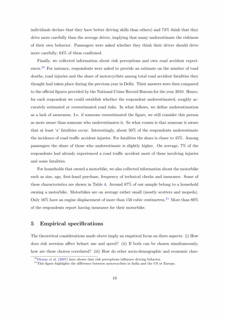
individuals declare that they have better driving skills than others) and 74% think that they

drive more carefully than the average driver, implying that many underestimate the riskiness

of their own behavior. Passengers were asked whether they think their driver should drive

more carefully; 64% of them confirmed.

Finally, we collected information about risk perceptions and own road accident experi-

ences.10 For instance, respondents were asked to provide an estimate on the number of road

deaths, road injuries and the share of motorcyclists among total road accident fatalities they

thought had taken place during the previous year in Delhi. Their answers were then compared

to the official figures provided by the National Crime Record Bureau for the year 2010. Hence,

for each respondent we could establish whether the respondent underestimated, roughly ac-

curately estimated or overestimated road risks. In what follows, we define underestimation

as a lack of awareness. I.e. if someone overestimated the figure, we still consider this person

as more aware than someone who underestimates it. So what counts is that someone is aware

that at least ‘x’ fatalities occur. Interestingly, about 50% of the respondents underestimate

the incidence of road traffic accident injuries. For fatalities the share is closer to 45%. Among

passengers the share of those who underestimate is slightly higher. On average, 7% of the

respondents had already experienced a road traffic accident most of these involving injuries

and some fatalities.

For households that owned a motorbike, we also collected information about the motorbike

such as size, age, first-hand purchase, frequency of technical checks and insurance. Some of

these characteristics are shown in Table 4. Around 87% of our sample belong to a household

owning a motorbike. Motorbikes are on average rather small (mostly scotters and mopeds).

Only 16% have an engine displacement of more than 150 cubic centimetres.11 More than 80%

of the respondents report having insurance for their motorbike.

5 Empirical specifications

The theoretical considerations made above imply an empirical focus on three aspects: (i) How

does risk aversion affect helmet use and speed? (ii) If both can be chosen simultaneously,

how are these choices correlated? (iii) How do other socio-demographic and economic char-

10Dionne et al. (2007) have shown that risk perceptions influence driving behavior.11This figure highlights the difference between motorcyclists in India and the US or Europe.

19

acteristics as well as behaviors and perceptions influence both helmet use and speed? In our

empirical analysis we propose two alternative ways of accounting for the simultaneity of the

two decisions: first to combine both choices in one categorial variable (the level of ‘protec-

tion’ hereafter) and second to model both choices separately, but to estimate them jointly to

account for the possible correlation of the residuals.

The level of protection is coded as follows: “no protection” (no helmet and high speed,

y = 1), “partial protection” (either only helmet or only low speed, y = 2) and “full protection”

(helmet and low speed, y = 3). To explore the role of risk aversion and other factors on the

chosen level of protection, we estimate an ordered logit model, which can be described as

follows.

The cumulative probability Cij gives the probability that the ith individual is in the jth

or higher category:

Cij = Pr(yi ≤ j) =

j∑cat=1

Pr(yi = k). (16)

This cumulative probability can be turned into the cumulative logit:

logit(Cij) = log( Cij

1− Cij

).

The ordered logit model represents the cumulative logit as a linear function of exogenous

variables xi:

logit(Cij) = aj − x′iβp, (17)

where aj indicates the logit of the odds of being equal to or less than category j for the

‘baseline’ group, i.e. when all xi are zero. Hence, these intercepts, or ‘cut-points’, increase

over j. The coefficients βp tell us how an increase in xi increases the log-odds of being higher

than category j. It is assumed that the effect of xi, i.e. βp does not vary with the cut-point

considered. Put differently, the marginal effect of risk aversion on the chosen protection level

for instance, does not vary whether a given individual has currently no or partial protection.

Again the second approach we use consists of unpacking the level of protection, and hence

considering two functions one for helmet use, hi and one for speed, si, but to estimate them

simultaneously. Helmet adoption is used in a binary form, i.e. the driver wears a helmet

20

(h = 1) or not (h = 0). Hence we use a simple probit model for estimation. Speed is

measured continuously (in kph) and we thus use a linear regression model.

Probit(hi = 1|xi) = θ(x′iβh + εhi), (18)

si = βs0 + x′iβs1 + εsi. (19)

We jointly estimate Equations (18) and (19) with full maximum likelihood, assuming that

the errors, εsi and εhi, follow a bivariate normal distribution, and then test the covariance of

the error terms.12 In the absence of convincing instruments we exclude speed from the helmet

equation and helmet use from the speed equation.

Again, for passengers we assume that only helmet use is a choice, which we model with a

simple probit model as described in Equation (18).

6 Empirical analysis and results

6.1 Drivers

6.1.1 The chosen level of protection and the role of risk aversion

The results of the ordered logit model are shown in Table 5. We start with a model in

which the only explanatory variable is risk aversion (col. (1)), then we introduce successively

socio-demographic and economic characteristics (col. (2)), religion (col. (3)) and driving

behavior and attitudes towards road safety issues (col. (4)). Augmenting the model step-by-

step allows us to see whether the estimated effects are sensitive to the inclusion and exclusion

of particular variables. As mentioned above, we also include here and in all estimations that

follow interviewer-effects.

Risk aversion has throughout a positive effect on protection, but is statistically only

significant if the full set of explanatory variables is included (col. (4)). Moreover the size

of the coefficient is also sensitive to the exact sample chosen. Risk aversion is significant

in column (5) which uses the same sample as column (4), but does not control for driving

behavior and safety perception.13 Overall, the effect of risk aversion is thus in line with the

12For estimation we use the STATA module ‘cmp’ developed by Roodman (2011), which can deal withconditional mixed process models.

13When we include variables that measure driving behavior and safety perceptions, we loose 116 observations

21

prediction in the model. In quantitative terms the estimated coefficient implies that at the

sample mean an increase by one standard deviation in the risk aversion score (+0.82 or 29%)

increases the probability that a driver will choose full protection by almost eight percentage

points (marginal effects are shown in the appendix). If we use risk aversion in each of the

four domains constituting our index, we find qualitatively the same effects. If we use other

measures such as the lottery questions and so on, we find either similar or insignificant results;

only for the questions regarding risk-taking behavior in business projects does the coefficient

have a significant opposite effect, but we do not consider this risk dimension as being very

relevant here (results not shown in Table).

Among the socio-demographic characteristics, it is interesting to see that the number of

children is positively associated with the level of protection. This may imply that drivers that

feel a responsibility towards a family choose a higher level of protection. Every additional child

increases the probability that the driver chooses full protection by seven to eight percentage

points (the effect is probably non-linear, as household size has a negative effect). Literacy

is also associated with a higher level of protection. Illiterate drivers have an approximate

25 percentage point lower probability of adopting the full protection compared to literate

drivers. The estimated income effects suggest that poorer individuals choose lower levels of

protection compared to richer individuals — in particular very rich individuals. Drivers with

a reported monthly household income of 25,000 INR and above (420 USD and more) have a

probability that is higher by 20 to 25 percentage points of choosing full protection compared

to drivers with a reported household income of less than 5,000 INR. In the middle income

range, the income gradient is almost flat.

Muslims relative to Hindus choose lower levels of protection, although the coefficient is

not significant throughout. The effects associated with the Sikh group are not significant,

although we have seen above that they show significantly lower levels of helmet use. As we

will see below, they also choose lower speed levels and hence the adverse effect of no helmet

use on protection is mitigated. We do not find, as one could expect, that those drivers who

think that their fate is in god’s hands choose lower levels of protection.

There is no difference between drivers that have already experienced an accident and

those who have not. We only find that drivers who never use ring roads choose higher levels

due to missing information.

22

of protection. As can be seen below, this has mainly to do with the lower speed chosen. The

choice of the road might even be part of the safety strategy: drivers decide to avoid ring roads

in order to travel at a lower speed, implying that “roads used” might be an endogenous deci-

sion variable. The effect associated with health insurance is also interesting. We do not find

any evidence of moral hazard: insured people are more likely, not less, to choose high levels

of protection. Finally, as already seen in our descriptive table above, drivers tend to chose

higher protection on long distance trips and lower protection on short distance trips. For a

long distance trip the probability of choosing full protection compared to a short distance

trip is about 15 percentage points higher.

[insert Table 5 here]

6.1.2 Unpacking protection: the choice of speed and helmet use

We now decompose the protection level adopted by the driver and consider the multidi-

mensional aspect of this behavior by looking at the exact strategy a driver opts for. We

thus investigate the relation between helmet use and average speed using the simultaneous

equations system described above. Here again, we successively expand the list of explanatory

variables. Using a longer list of variables again implies working with a slightly smaller sample.

In all specifications we control for interviewer-effects.

Risk aversion is positively associated with helmet use. This effect is relatively robust.

At the sample mean, a one standard deviation increase in the risk aversion measure (i.e. by

0.82 points or 29%) increases the probability of helmet use by roughly 3 percentage points.

However, risk aversion does not have a significant impact on speed. This is coherent with the

predictions of our theoretical model. Risk averse individuals engage in self-insurance, but the

effect on self-protection is ambiguous. These results also largely hold if we estimate separately

by the type of trip. They are also confirmed if we take risk-taking behavior in each domain

alone. If we take the other risk-measures in our data set we find insignificant results except for

one of the lottery-based measures and the measure based on the risky medicine question for

which risk-aversion seems to lower the probability of helmet use (results not shown in Table).

Again, we trust our self-reported risk measures more. We also obtain absolutely coherent

results if, instead of the binary helmet variable, we use the combined helmet and strap use

23

(5 categories, see Table 2). The effects of the other explanatory variables are largely in line

with our findings in Table 5, where we analyzed protection, i.e. helmet and speed combined.

Helmet use is lower among the illiterate population, between 10 to 12 percentage points

depending on the specification. Tertiary education seems to further increase the probability

of helmet use, but this effect loses significance if religiousness and social status is added to the

list of regressors. Sikhs are, for the reasons given above, less likely to wear a helmet (17 to

20 percentage points less likely), but they also drive on average slower (8 to 10 kph less (4 to

6 mph)) and thus seem to compensate their increased exposure to risk. For that group, not

wearing a helmet is not necessarily the preferred choice, but rather a (religious) constraint

and hence risk compensation can be a rational response. The more children a driver has the

lower the chosen speed level (roughly 3 kph (1.9 mph) less per child), however, more children

is not associated with a higher probability of helmet use. Income also does not correlate

with helmet use conditional on all other included variables, however it plays a role for speed.

The results suggest that speed first increases and then decreases with income. Drivers with

a monthly household income of more than 25,000 INR drive on average 15 to 25 kph (9 to 16

mph) slower than drivers with a monthly household income of 10,000 to 15,000 INR. Here it

is important to note that the size of the motorbike is controlled (engine displacement).

Among the variables measuring driving behavior and safety perceptions, a few effects

stand out. Drivers who use their motorbike regularly to commute to work are more likely to

wear a helmet (+6 percentage points). There is no effect on speed. Risk awareness seems

to matter: drivers who took driving lessons are more likely to wear a helmet (+7 percentage

points). Interestingly, individuals who have a driving license but did not take driving lessons

are not more likely to use a helmet than those who don’t have a license at all (effect not shown

in Table 6). Again, this suggests that it is awareness that matters. Drivers who underestimate

the annual number of road traffic accident injuries, and thus the implied risk more generally,

are less likely to wear a helmet. More passengers on the motorbike is also associated with

lower helmet use. Remarkably, drivers with health insurance are more likely to wear a helmet

and to drive slower. Note that this result holds even if we control for income, education and

a whole range of other characteristics.

Finally, since we estimate helmet use and the choice of speed with a simultaneous equation

system, it is interesting to examine the correlation between the error terms of both equations.

24

The error terms capture those determinants that are not included in the list of regressors

and of course measurement error. If we control only for risk aversion (col. (1)), the error

terms are significantly negatively correlated, implying that the net effect of the unobserved or

not included factors tends to increase helmet use and to lower speed, or, in turn to decrease

helmet use and to increase speed. As more and more explanatory variables are included (col.

(2) and col. (3)), we see that the correlation remains significantly negative and even increases

in absolute size. If we include those variables that account for driving behavior and safety

perceptions (col. (4)), we see that the correlation coefficient loses its significance. This is not

due to the reduced sample size, as col. (5) shows, where we re-estimate the regression on the

same sample without controlling for driving behavior and safety perceptions. As discussed

above, among the variables measuring driving behavior and safety perceptions, of particular

significance in both equations are those that can be related to risk awareness, such as taking

driving lessons, underestimating the number of annual fatalities and having an insurance.

Put differently, given that we control (even if imperfectly) for risk aversion and a large set of

socio-demographic and economic characteristics including religiousness, we believe that risk

awareness is a major determinant that can explain whether individuals wear a helmet and

drive slowly or do not wear a helmet and drive fast. Hence, whereas risk aversion motivates

drivers to compensate for higher speed through a higher propensity to use a helmet, a lack of

awareness comes with both, high speed and no helmet, i.e. both decisions seem to complement

each other. All our results are qualitatively not different if we limit the sample to those drivers

that own a helmet (not shown in Table).

[insert Table 6 here]

6.2 Passengers

Again, for passengers we assume that they only make a choice regarding helmet use and

consider speed to be determined by the driver, although there might be possibilities for the

passenger to influence the driver to some extent. This is discussed in more detail below. Table

7 shows the results. We only present marginal effects.

[insert Table 7 here]

25

Interestingly, for passengers we do not find any significant effect for risk aversion if we use

our risk aversion score. However, we do find some significant positive effects when using the

risky medicine question; nevertheless, for other risk aversion measures, in particular lottery

questions, again the effects are negative (results not shown in Table), so no clear-cut conclusion

can be drawn for passengers.

One of the most important determinants of helmet use among passengers is gender. Men

are between 25 to 40 percentage points more likely to wear a helmet than women, controlling

for all other socio-demographic and economic characteristics and differences in travel habits

and safety perceptions. Some of the factors driving this result have already been discussed

above. Women are exempted from the helmet law. Moreover, women may refuse to wear a

helmet because of their hair-dress. Nevertheless according to our data (cf. Table 2), 45% of

all women always wear a helmet at least on long trips. On short trips this share is still at

15%. We also test whether owning a helmet makes a difference, even though this variable is

of course highly endogenous. Owning a helmet increases the probability of wearing a helmet

by about 30 percentage points. The gender effect is strongly reduced in the specification with

helmet ownership.However, given the low cost of and easy access to helmets, we believe that

there is no difference in modelling the decision to use and the decision to buy a helmet.

Religiousness and whether a passenger believes that life is in the hands of a superior force

does not explain helmet use. Although the coefficient associated with the latter variable is

negative throughout, it is never statistically significant. Education and income also seem

to play no role. The same is true for marital status, having children and household size.

However, being of a lower caste decreases helmet use, by 8 to 15 percentage points.

Based on the predictions derived from our theoretical model, we expect a negative corre-

lation between helmet use and exogenous improvements in the safety level (the “Peltzman-

effect”). In Table 7 we do indeed see that the passenger’s choice to wear a helmet is influenced

by the driver’s choice of speed. Helmet use increase with speed, at least if a speed below 20

kph is compared to a speed between 20 and 40 kph (12 and 25 mph).

As with drivers, we again find that people who underestimate the risk of a road traffic

accident wear a helmet less often (10 to 15 percentage points less likely). Surprisingly, for

passengers, in contrast to drivers, we find that passengers with health insurance wear a helmet

less often (12 percentage points less likely). It could be that for passengers there is some moral

26

hazard, in a sense that passengers think better health care reduces the cost of an injury, but

this is a strong hypothesis that needs further empirical testing. Finally, we see that passengers

who think their driver is speeding too much and who hence may urge their driver to pay more

attention, wear a helmet less often (9 to 12 percentage points less likely). This may imply that

passengers try to reduce the probability of accident involvement by influencing the driver’s

chosen level of speed. This result can also be seen as evidence of a ‘Peltzman effect’ as it

reflects a trade-off between the passenger’s and driver’s safety efforts.

7 Conclusion

Risky health behavior is in many domains still only poorly understood. The analysis is

often plagued by incomplete data and a general lack of information. In this study, we try

to understand the behavior of helmet use among motorcycle riders and passengers in Delhi,

a context in which road safety is low and helmet use is far from being the norm. We use a

very detailed data set collected exactly for the purpose of that study. To guide our empirical

analysis, we rely on a simple model in which drivers decide on their speed and helmet use.

While a helmet provides insurance if an accident happens, speed affects the probability that

an accident will occur. However, a lower speed implies time costs and helmet use comes with

a level of discomfort that has to be borne by the user. Key variables in our analysis are risk

aversion as well as aspects related to risk awareness.

The empirical findings suggest that risk averse drivers are more likely to wear a helmet.

A one standard deviation increase in our risk aversion score (i.e. by 29%) increases the

probability of using a helmet on a given trip by 3 percentage points. This is certainly not a

very strong effect, but cumulated over many trips it means a substantial reduction in the risk

of being seriously injured in the event of an accident. We do not find any systematic effect of

risk aversion on speed. Both results are coherent with our theoretical model. Interestingly,

helmet use also increases with education: illiterate drivers are by about 10% less likely to

wear a helmet than literate drivers. Tertiary education further increases helmet use. Speed

decreases with the number of children at home suggesting that family responsibilities stimulate

drivers to take fewer risks. Speed first increases and then decreases with income, i.e. the

middle class drives the fastest.

Drivers who show a higher awareness of road risks, because, for instance, they are more

27

conscious about the health risks faced when traveling on Delhi’s roads or have taken driving

lessons, are both more likely to wear a helmet and to speed less. In turn, those drivers who

show a high level of unawareness take the highest risks. Controlling for risk awareness, we

observe that drivers tend to compensate between speed and helmet use: the Sikh who cannot

wear a helmet because of the turban, drive, on average, slower.

For passengers, we find a similar pattern. Their probability of helmet use increases with

the driver’s chosen level of speed. The fact that generally passengers less often wear a helmet

than drivers, and women less often than men, even controlling for helmet ownership, suggests

that norms and habits also play an important role. Breaking these is one of the major

challenges that needs to be overcome.

The most obvious solution to India’s road safety problem and the related high social

costs that result from it, is to enforce the helmet law and speed limits and hence to ignore

the associated private costs such as time costs and discomfort. An alternative strategy, and

probably more feasible in the current context, is to design interventions which raise awareness

of road risks. In terms of our model, this means bringing the expected probability of an

accident at a given speed and the expected gain of helmet use closer to its actual levels.

Improvements to the road infrastructure such as separate lanes for cars and motorbikes are

also a possible solution, but, as our analysis and a few other examples in the literature show,

these measures bear the risk that drivers will react by increasing speed or lowering helmet

use.

We end our analysis with a word of caution. In this study we work with purely obser-

vational data and hence we cannot really claim to tease out causal relationships. However,

given the detail of the information we have, we think there are good reasons to believe that

biases due to omitted variables are relatively limited. Further research should try to validate

some of the findings we generated through an adequate experimental design. Nevertheless, we

believe that our analysis is a first important step in understanding helmet use in a low-income

but highly-motorized context.

28

Appendix

Determinants of non-reporting

[insert Table A1 here]

Marginal effects

[insert Tables A2 and A3 here]

Acknowledgements

We thank SIGMA Research and Consulting for excellent collaboration in the field. We are

also grateful to Arjun Bedi, Denis Cogneau, Pierre-Yves Geoffard, Robert Sparrow, Lara

Tobin, Armando Treibich and Rafael Treibich for very valuable comments on this version.

Thanks are also due to seminar participants at Linz University, Erasmus University Rotter-

dam, Passau University, Universite Paris Dauphine, the Paris School of Economics and the

Aix-Marseille School of Economics and participants of the Development Economics Confer-

ence of the German Economic Association in Munich and of the “Research in Health and

Labour” TEPP Conference in Le Mans. Financial support for this research from the Health

Chair - a joint initiative by PSL, Universite Paris-Dauphine, ENSAE and MGEN under the

aegis of the Fondation du Risque (FDR) - the Paris School of Economics Research Fund and

the International Institute of Social Studies of Erasmus University Rotterdam is gratefully

acknowledged.

References

Levon Barseghyan, Jeffrey Prince, and Joshua C. Teitelbaum. Are risk preferences stable

across contexts? evidence from insurance data. American Economic Review, 101(2):591–

631, 2011.

Soma Bhattacharya, Anna Alberini, and Maureen L. Cropper. The value of mortality risk

reductions in delhi, india. Journal of Risk and Uncertainty, 34:21–47, 2007.

29

Glenn Blomquist. A utility maximization model of driver traffic safety behavior. Accident

Analysis and Prevention, 18(5):371–375, October 1986.

Eric Bryis and Harris Schlesinger. Risk aversion and the propensities for self-insurance and

self-protection. Southern Economic Journal, 57(2):458–467, October 1990.

Robert S. Chirinko and Edward P. Harper Jr. Buckle up or slow down? new estimates

of offsetting behavior and their implications for automobile safety regulation. Journal of

Policy Analysis and Management, 12(2):270–296, 1993.

Thomas S. Dee. Motorcycle helmets and traffic safety. Journal of Health Economics, 28:

398–412, 2009.

Xiaohao Ding, Joop Hartog, and Yuze Sun. Can we measure individual risk attitudes in a

survey? IZA Discussion Paper Series 4807, Bonn, March 2010.

Georges Dionne and Louis Eeckhoudt. Self-insurance, self-protection and increased risk aver-

sion. Economic Letters, 17(1-2):39–42, 1985.

Georges Dionne, Claude Fluet, and Denise Desjardins. Predicted risk perception and risk-

taking behavior: The case of impaired driving. Journal of Risk and Uncertainty, 35:237–264,

2007.

Thomas Dohmen, Armin Falk, David Huffman, Uwe Sunde, Jurgen Schupp, and Gert G.

Wagner. Individual risk attitudes: Measure, determinants, and behavioral consequences.

Journal of the European Economic Association, 9(3):522–550, June 2011.

Isaac Ehrlich and Gary S. Becker. Market insurance, self-insurance and self-protection. Jour-

nal of Political Economy, 80:623–648, 1972.

Liran Einav, Amy Finkelstein, Iuliana Pascu, and Mark R. Cullen. How general are risk

preferences? choices under uncertainty in different domains. American Economic Review,

102(6):2606–2538, 2012.

Michael T. French, Gulcin Gumus, and Jenny F. Homer. Public policies and motorcycle

safety. Journal of Health Economics, 28:831–838, 2009.

30

Jonathan P. Goldstein. Self-insurance: The case of motorcycle helmets. The Journal of Risk

and Insurance, 63(2):313–322, June 1996.

Michael Grimm and Carole Treibich. Determinants of road traffic crash fatalities across indian

states. Health Economics, 22(8):915–930, August 2013.

Bernd Hardeweg, Lukas Menkhoff, and Hermann Waibel. Experimental validated survey

evidence on individual risk attitudes in rural thailand. Discussion Paper No 464, April

2012.

Arvind Kumar, Sanjeev Lalwani, Deepak Agrawal, Ravi Rautji, and TD. Dogra. Fatal road

traffic accidents and their relationship with head injuries: An epidemiological survey of five

years. Indian Journal of Neurotrauma, 5(2):63–67, 2008.

Kangoh Lee. Risk aversion and self-insurance-cum-protection. Journal of Risk and Uncer-

tainty, 17:139–150, 1998.

BC. Liu, R. Ivers, R. Norton, S. Boufous, S. Blows, and SK. Lo. Helmets for preventing

injury in motorcycle riders. Cochrane Database of Systematic Reviews, 1, 2008.

Alan D. Lopez, Colin D. Mather, Majid Ezzati, Dean T. Jamison, and Christopher JL.

Murray. Global and regional burden of disease and risk factors, 2001: systematic analysis

of population health data. The Lancet, 367(9524):1747–1757, May 2006.

Adrian K. Lund and Brian O’Neill. Perceived risks and driving behavior. Accident Analysis

and Prevention, 18(5):367–370, 1986.

Adrian K. Lund and Paul Zador. Mandatory belt use and driver risk taking. Risk Analysis,

4(1):41–53, 1984.

Georg Lutz and Oliver Lipps. How answers on political attitudes are shaped by interviewers:

Evidence from a panel survey. Swiss Sociological Review, 36(2):345–358, 2010.

Patrick McCarthy and Wayne K. Talley. Evidence on risk compensation and safety behaviour.

Economic Letters, 62:91–96, 1999.

31

Antoine Messiah, Aymery Constant, Benjamin Contrand, Marie-Line Felonneau, and Lagarde

Emmanuel. Risk compensation: A male phenomenon? results from a controlled interven-

tion trial promoting helmet use among cyclists. American Journal of Public Health, 102:

S204–S206, 2012.

Dinesh Mohan. Social cost of road traffic crashes in india. In Proceedings First Safe Commu-

nity Conference on Cost of Injury, pages 33–38, October 2002.

Sam Peltzman. The effects of automobile safety regulation. Journal of Political Economy, 83

(4):677–726, August 1975.

Steven Peterson, George Hoffer, and Edward Millner. Are drivers of air-bag-equipped cars

more agressive? a test of the offsetting behavior hypothesis. Journal of Law and Economics,

38(2):251–264, October 1995.

John W. Pratt. Risk aversion in the small and in the large. Econometrica, 32(1/2):122–136,

January-April 1964.

David Roodman. Fitting fully observed recursive mixed-process models with cmp. Stata

Journal, 11(2):159–206, 2011.

Russel S. Sobel and Todd M. Nesbit. Automobile safety regulation and the incentive to drive

recklessly: Evidence from nascar. Southern Economic Journal, 74(1):71–84, July 2007.

Adam Stetzer and David A. Hofmann. Risk compensation: Implications for safety interven-

tions. Organizational Behavior and Human Decision Processes, 66(1):73–88, April 1996.

Marjon van der Pol and Matteo Ruggeri. Is risk attitude outcome specific within the health

domain? Journal of Health Economics, 27:706–717, 2008.

WHO. World report on road traffic injury prevention. Technical report, World Health Orga-

nization, 2004.

WHO. Helmets: a road safety manual for decision-makers and practitioners. Technical report,

World Health Organization, 2006.

WHO. Global status report on road safety. Technical report, World Health organization,

2009.

32

Gerald J. S. Wilde. The theory of risk homeostasis: Implications for safety and health. Risk

Analysis, 2(4):209–225, 1982.

Eva Wolbert and Arno Riedl. Measuring time and risk preferences: Reliability, stability,

domain specificity. CESifo Working Paper 4339, Munich, July 2013.

33

Tables

Table 1: Socio-demographic characteristics of drivers and passengers

Male Passengers All(%) drivers Male Female respondents

Male - - - 67.41Age distribution15-29 years 37.83 32.26 27.70 34.9230-39 years 25.36 13.98 32.37 26.0540-49 years 20.25 15.05 25.18 20.8450-59 years 11.25 17.20 8.99 10.9860 years and above 5.32 21.51 5.76 7.21Average (in years) 35.44 42.10 37.00 36.47Married 69.34 68.82 85.56 73.39Contributes to HH income 80.78 68.78 5.80 55.00Share of the contributionless than 40% 32.09 44.09 96.01 54.59between 40% and 60% 19.67 22.58 3.62 14.77more than 60% 48.24 33.33 0.36 30.65Education levelilliterate 2.49 7.53 14.75 6.95primary school 3.53 11.83 4.73 4.93secondary school 48.55 65.59 49.09 50.34tertiary education 45.44 15.05 30.94 37.78ReligionHindu 83.44 86.02 86.69 84.37Muslim 12.07 10.75 9.35 11.09Sikh 1.23 2.15 3.24 3.44other 3.27 1.08 0.72 1.11Prays daily 65.30 74.19 80.73 71.24Believes fate is in god’s hands 87.50 90.22 87.27 88.18

Has health insurance 15.11 11.83 12.64 13.77Observations 489 93 278 902

Notes: The group “all respondents” includes 27 individuals that declared to be

sometimes driver and sometimes passenger as well as 15 female drivers. Both

groups are not included in any of the sub-samples.

Table 2: Helmet use and other safety behaviors by type of user and gender

Male Passengers Alldrivers Male Female respondents

HELMET CHARACTERISTICS (%)Helmet ownershipyes 93.24 51.61 56.20 76.92Observations 488 93 274 897Type of helmetfull face helmet 86.49 82.98 65.77 80.68open face helmet 6.08 2.13 6.04 6.09half helmet 6.98 14.89 27.52 12.78building site helmet 0.45 0 0.67 0.45Condition of the helmetgood condition 72.93 74.47 79.33 74.59some scratches 25.95 25.53 20.00 24.22broken but manually fixed 1.12 0 0.67 1.18Helmet with strapyes 97.75 93.75 93.42 96.49Observations 447 47 152 684

HELMET USE (%)In neighbourhoodsyes 73.80 48.91 20.15 54.41For short trips on main roadsyes 79.84 48.39 30.97 60.97For long trips on main roadsyes 96.88 83.87 52.08 81.14Observations 481 93 268 884

OTHER SAFETY BEHAVIORSSpeed (kph)a

average 36.67 30.64 29.58 33.83variance 21.56 17.47 17.28 20.53Observations 410 73 170 686

Notes: The group “all respondents” includes 27 individuals that declared to be sometimes

driver and sometimes passenger as well as 15 female drivers. Both groups are not included

in any of the sub-samples. a) observations with a declared speed of more than 150 kph are

excluded.

Table 3: Probability of engaging in risky health behaviors, linear probability model

Smoking Drinking Drinking heavilya

Risk aversion score -0.036?? -0.035?? -0.024??

(0.016) (0.014) (0.12)Interviewer fixed effects yes yes yes

R2 0.275 0.195 0.245Observations 832 807 806

Notes: ? p<0.10, ?? p<0.05, ??? p<0.01. Sample of all respondents.

OLS estimations. Robust standard errors are reported in parentheses.

a) had three alcoholic beverages in a row at least once in the past

two weeks.

Table 4: Driving behaviors and risk awareness

Male Passengers Alldrivers Male Female respondents

DRIVING BEHAVIORS (%)Road exposureUses motorbike to commute (=1) 83.37 67.74 29.96 76.92Never uses ring roads (=1) 12.92 16.09 24.23 16.53Observations 487 93 277 897# of persons on motorbike 1.42 2.46 2.72 1.95Observations 478 87 267 869Driving skillsConfident in own driving ability (=1) 55.94Reports driving more carefully than others (=1) 74.18Formal trainingHas a driving licence (=1) 91.45Took driving lessons (=1) 42.36Took a driving exam (=1) 65.44Observations 488Says own driver should pay more attention (=1) 56.06 67.00Observations 66 200SAFETY PERCEPTIONS (%)Experienced road trafic accident (=1) 9.67 8.79 2.17 7.15Observations 486 91 277 895AwarenessUnderest. Annual road injuries (=1) 50.06 60.81 55.05 53.45Underest. Annual road deaths (=1) 42.76 49.35 41.18 43.43Observations 442 77 221 769MOTORBIKE CHARACTERISTICS (%)HH owns a motorbike (=1) 92.62 48.39 90.65 87.35Observations 488 93 278 901Size of the motorbikeLess than 100cc 28.07 30.00 32.58 29.45Between 100cc and 150cc 54.52 57.50 53.39 54.52Above 150cc 17.40 12.50 14.03 16.03Observations 431 40 221 730Has motorbike insurance (=1) 80.96 85.71 82.25 81.61Observations 436 42 231 745

Notes: The group “all respondents” includes 27 individuals that declared to be sometimes

driver and sometimes passenger as well as 15 female drivers. Both groups are not included

in any of the sub-samples.

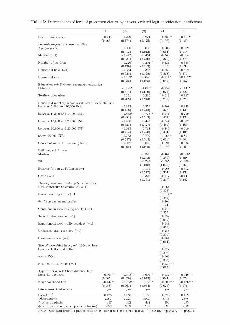
Table 5: Determinants of level of protection chosen by drivers, ordered logit specification, coefficients

(1) (2) (3) (4) (5)

Risk aversion score 0.244 0.229 0.274 0.386?? 0.411??

(0.163) (0.174) (0.175) (0.197) (0.189)Socio-demographic characteristicsAge (in years) 0.008 0.006 0.006 0.002

(0.012) (0.012) (0.014) (0.013)Married (=1) -0.422 -0.464 -0.263 -0.314

(0.331) (0.340) (0.375) (0.370)Number of children 0.276?? 0.292?? 0.321?? 0.355???

(0.120) (0.122) (0.130) (0.133)Household head (=1) -0.354 -0.357 -0.583 -0.612

(0.325) (0.328) (0.378) (0.375)Household size -0.102? -0.090 -0.111? -0.117??

(0.055) (0.055) (0.059) (0.057)Education ref: Primary-secondary educationIlliterate -1.195? -1.076? -0.959 -1.141?

(0.614) (0.646) (0.675) (0.622)Tertiary education 0.251 0.210 0.083 0.167

(0.209) (0.214) (0.231) (0.226)Household monthly income, ref: less than 5,000 INRbetween 5,000 and 10,000 INR -0.313 -0.259 -0.398 -0.345

(0.418) (0.413) (0.477) (0.448)between 10,000 and 15,000 INR -0.843?? -0.773?? -0.571 -0.700

(0.381) (0.392) (0.463) (0.439)between 15,000 and 20,000 INR -0.498 -0.449 -0.247 -0.357

(0.423) (0.427) (0.481) (0.460)between 20,000 and 25,000 INR -0.615 -0.718? -0.445 -0.519

(0.414) (0.420) (0.464) (0.435)above 25,000 INR 0.753 0.709 1.064? 0.801

(0.537) (0.543) (0.621) (0.604)Contribution to hh income (share) -0.047 -0.046 -0.021 -0.035

(0.095) (0.095) (0.107) (0.104)Religion, ref: HinduMuslim -0.325 -0.461 -0.508?

(0.292) (0.330) (0.308)Sikh -0.742 -1.055 -1.055

(1.018) (1.056) (1.060)Believes fate in god’s hands (=1) 0.156 0.068 0.312

(0.317) (0.364) (0.334)Caste (=1) -0.325 -0.117 -0.141

(0.231) (0.247) (0.242)Driving behaviors and safety perceptionsUses motorbike to commute (=1) 0.061

(0.328)Never uses ring roads (=1) 1.017??

(0.439)# of persons on motorbike -0.304

(0.194)Confident in own driving ability (=1) -0.275

(0.257)Took driving lessons (=1) 0.192

(0.250)Experienced road traffic accident (=1) -0.148

(0.456)Underest. ann. road inj. (=1) -0.258

(0.261)Owns motorbike (=1) -0.951

(0.614)Size of motorbike in cc, ref: 100cc or lessbetween 100cc and 150cc -0.177

(0.297)above 150cc 0.163

(0.382)Has health insurance (=1) 0.039???

(0.013)Type of trips, ref: Short distance tripLong distance trip 0.564??? 0.598??? 0.601??? 0.687??? 0.646???

(0.065) (0.070) (0.072) (0.084) (0.079)Neighbourhood trip -0.147?? -0.163?? -0.168??? -0.200??? -0.186???

(0.058) (0.063) (0.064) (0.075) (0.071)Interviewer fixed effects yes yes yes yes yes

Pseudo R2 0.125 0.158 0.168 0.223 0.189Observations 1369 1324 1294 1178 1178# of respondents 457 442 432 393 393# of observations per respondent (mean) 2.99 2.99 2.99 2.99 2.99

Notes: Standard errors in parentheses are clustered at the individual level. ? p<0.10, ?? p<0.05, ??? p<0.01.

Table 6: Helmet use and speed level chosen by drivers, simultaneous equation system, coeffi-cients

(1) (2) (3) (4) (5)

HELMET USE (Probit)Risk aversion score 0.165 0.152 0.208? 0.229? 0.327???

(0.113) (0.118) (0.118) (0.134) (0.124)Socio-demographic characteristicsAge (in years) -0.005 -0.000 0.006 -0.002

(0.009) (0.010) (0.009) (0.010)Married (=1) 0.145 0.180 0.195 0.180

(0.237) (0.252) (0.288) (0.265)Number of children 0.082 0.034 0.008 0.078

(0.079) (0.076) (0.086) (0.083)Household head (=1) 0.171 0.155 0.051 0.001

(0.242) (0.255) (0.272) (0.286)Household size -0.082?? -0.076?? -0.110??? -0.094???

(0.034) (0.034) (0.038) (0.036)Education, ref: Primary-secondary educationIlliterate -0.749??? -0.639?? -0.662? -0.670??

(0.249) (0.285) (0.363) (0.301)Tertiary education 0.305?? 0.235 0.156 0.226

(0.142) (0.144) (0.158) (0.147)Household monthly income, ref: less than 5,000 INRbetween 5,000 and 10,000 INR -0.264 -0.172 -0.270 -0.163

(0.278) (0.269) (0.296) (0.302)between 10,000 and 15,000 INR -0.397 -0.258 -0.299 -0.204

(0.257) (0.253) (0.265) (0.279)between 15,000 and 20,000 INR 0.066 0.104 0.037 0.165

(0.306) (0.305) (0.328) (0.339)between 20,000 and 25,000 INR 0.133 0.166 0.460 0.571

(0.331) (0.348) (0.347) (0.355)above 25,000 INR 0.377 0.348 0.285 0.397

(0.399) (0.414) (0.539) (0.452)Contribution to hh income (share) -0.004 -0.004 -0.004 0.007

(0.059) (0.060) (0.065) (0.064)Religion, ref: HinduMuslim -0.012 -0.152 -0.220

(0.224) (0.247) (0.232)Sikh -1.207??? -1.117??? -1.071???

(0.403) (0.394) (0.398)Believes fate in god’s hands (=1) -0.095 -0.242 -0.050

(0.214) (0.284) (0.245)Caste (=1) -0.245? -0.037 -0.169

(0.146) (0.156) (0.154)Driving behaviors and safety perceptionsUses motorbike to commute (=1) 0.398?

(0.230)Never uses ring roads (=1) 0.037

(0.234)# of persons on motorbike -0.297??

(0.119)Confident in own driving ability (=1) -0.152

(0.179)Took driving lessons (=1) 0.434??

(0.187)Underest. ann. road inj. (=1) -0.428??

(0.189)Experienced road traffic accident (=1) -0.039

(0.258)Owns motorbike (=1) -0.074

(0.371)Size of motorbike in cc, ref: 100cc or lessbetween 100cc and 150cc 0.055

(0.193)above 150cc 0.349

(0.255)Has motorbike insurance (=1) -0.023

(0.233)Has health insurance (=1) 0.020??

(0.008)Type of trips, ref: Short distance tripLong distance trip 1.190??? 1.276??? 1.340??? 1.648??? 1.531???

(0.147) (0.150) (0.157) (0.183) (0.188)Neighbourhood trip -0.194??? -0.237??? -0.255??? -0.319??? -0.284???

(0.072) (0.079) (0.081) (0.094) (0.089)

(continues next page)

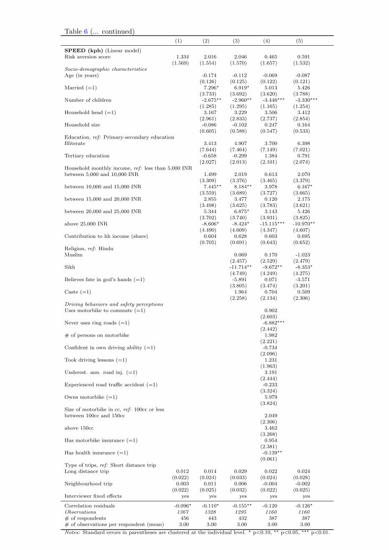
Table 6 (... continued)(1) (2) (3) (4) (5)

SPEED (kph) (Linear model)Risk aversion score 1.334 2.016 2.046 0.465 0.591

(1.569) (1.554) (1.570) (1.657) (1.532)Socio-demographic characteristicsAge (in years) -0.174 -0.112 -0.069 -0.087

(0.126) (0.125) (0.122) (0.121)Married (=1) 7.296? 6.919? 5.013 5.426

(3.733) (3.692) (3.620) (3.788)Number of children -2.675?? -2.960?? -3.446??? -3.330???

(1.285) (1.295) (1.165) (1.254)Household head (=1) 3.167 3.229 3.506 3.412

(2.961) (2.833) (2.737) (2.854)Household size -0.086 -0.102 0.247 0.164

(0.605) (0.588) (0.547) (0.533)Education, ref: Primary-secondary educationIlliterate 3.413 4.907 3.700 6.398

(7.644) (7.464) (7.149) (7.021)Tertiary education -0.658 -0.299 1.384 0.791

(2.027) (2.013) (2.101) (2.074)Household monthly income, ref: less than 5,000 INRbetween 5,000 and 10,000 INR 1.499 2.019 0.613 2.070

(3.309) (3.376) (3.465) (3.379)between 10,000 and 15,000 INR 7.445?? 8.184?? 3.978 6.167?

(3.559) (3.689) (3.727) (3.665)between 15,000 and 20,000 INR 2.855 3.477 0.120 2.175

(3.498) (3.625) (3.783) (3.621)between 20,000 and 25,000 INR 5.344 6.875? 3.143 5.426

(3.702) (3.740) (3.931) (3.825)above 25,000 INR -8.606? -8.424? -15.115??? -10.970??

(4.490) (4.609) (4.347) (4.607)Contribution to hh income (share) 0.604 0.628 0.603 0.695

(0.705) (0.691) (0.643) (0.652)Religion, ref: HinduMuslim 0.069 0.170 -1.023

(2.457) (2.529) (2.479)Sikh -11.714?? -9.672?? -8.353?

(4.749) (4.249) (4.275)Believes fate in god’s hands (=1) -5.891 0.071 -3.571

(3.805) (3.474) (3.201)Caste (=1) 1.964 0.704 0.509

(2.258) (2.134) (2.306)Driving behaviors and safety perceptionsUses motorbike to commute (=1) 0.902

(2.603)Never uses ring roads (=1) -6.882???

(2.442)# of persons on motorbike 1.982

(2.221)Confident in own driving ability (=1) -0.734

(2.096)Took driving lessons (=1) 1.231

(1.963)Underest. ann. road inj. (=1) 3.191

(2.444)Experienced road traffic accident (=1) -0.233

(3.324)Owns motorbike (=1) 5.979

(3.824)Size of motorbike in cc, ref: 100cc or lessbetween 100cc and 150cc 2.049

(2.306)above 150cc 3.462

(3.268)Has motorbike insurance (=1) 0.954

(2.381)Has health insurance (=1) -0.139??

(0.061)Type of trips, ref: Short distance tripLong distance trip 0.012 0.014 0.029 0.022 0.024

(0.022) (0.024) (0.033) (0.024) (0.028)Neighbourhood trip 0.003 0.011 0.006 -0.004 -0.002

(0.022) (0.025) (0.032) (0.022) (0.025)Interviewer fixed effects yes yes yes yes yes

Correlation residuals -0.096? -0.110? -0.155?? -0.120 -0.126?

Observations 1367 1328 1295 1160 1160# of respondents 456 443 432 387 387# of observations per respondent (mean) 3.00 3.00 3.00 3.00 3.00

Notes: Standard errors in parentheses are clustered at the individual level. ? p<0.10, ?? p<0.05, ??? p<0.01.

Table 7: Determinants of helmet use for passengers, probit specification, marginal effects

(1) (2) (3) (4) (5) (6) (7) (8)

Risk aversion score -0.063 -0.056 -0.067 -0.019 -0.054 -0.014 -0.019 -0.057(0.040) (0.044) (0.046) (0.034) (0.040) (0.033) (0.021) (0.049)

Speed, ref: between 20 and 40 kphbelow 20 kph -0.114? -0.093?

(0.064) (0.054)above 40 kph -0.063 -0.042

(0.062) (0.050)Owns a helmet (=1) 0.314???

(0.120)Socio-demographic characteristicsAge (in years) -0.003 -0.003 -0.003? -0.003? -0.002 -0.004?

(0.002) (0.002) (0.002) (0.002) (0.001) (0.002)Male (=1) 0.412??? 0.426??? 0.401??? 0.405??? 0.242?? 0.429???

(0.076) (0.075) (0.111) (0.110) (0.108) (0.082)Married (=1) 0.047 0.051 0.049 0.045 0.023 0.071

(0.066) (0.069) (0.053) (0.052) (0.033) (0.080)Number of children -0.009 0.003 0.008 0.007 0.007 0.008

(0.024) (0.025) (0.018) (0.018) (0.011) (0.027)Household head (=1) -0.088 -0.073 -0.034 -0.051 -0.031 -0.082

(0.085) (0.087) (0.069) (0.065) (0.040) (0.092)Household size 0.013 0.009 0.003 0.003 0.000 0.003

(0.011) (0.011) (0.009) (0.009) (0.005) (0.012)Education, ref: Primary-secondary educationIlliterate -0.102 -0.082 -0.068 -0.057 -0.021 -0.077

(0.081) (0.084) (0.059) (0.059) (0.036) (0.089)Tertiary education -0.070 -0.093 -0.071 -0.069 -0.020 -0.112

(0.060) (0.062) (0.053) (0.052) (0.029) (0.069)Household monthly income, ref: less than 10,000 INRbetween 10,000 and 20,000 INR -0.062 -0.057 -0.013 -0.011 -0.021 -0.021

(0.062) (0.063) (0.051) (0.050) (0.029) (0.069)above 20,000 INR 0.059 0.026 0.001 0.018 -0.037 -0.007

(0.090) (0.090) (0.069) (0.071) (0.038) (0.102)Religion, ref: HinduMuslim 0.033 0.035 0.019 0.024 0.061

(0.094) (0.077) (0.073) (0.050) (0.103)Sikh -0.025 -0.045 -0.025 -0.056 -0.011

(0.128) (0.067) (0.069) (0.037) (0.127)Believes fate in god’s hands (=1) -0.046 -0.039 -0.017 -0.024 -0.058

(0.090) (0.084) (0.076) (0.052) (0.106)Caste (=1) -0.110?? -0.090? -0.087? -0.042 -0.145??

(0.055) (0.048) (0.047) (0.033) (0.060)Driving behaviors and safety perceptionsUses motorbike to commute(=1) -0.010 -0.010 -0.018

(0.050) (0.048) (0.026)Never uses ring roads (=1) 0.035 0.059 0.027

(0.067) (0.071) (0.044)Size of motorbike in cc, ref: 100cc or lessbetween 100cc and 150cc 0.077 0.077 0.024

(0.053) (0.053) (0.035)above 150cc 0.222 0.195 0.060

(0.137) (0.133) (0.081)Experienced road traffic accident (=1) -0.081 -0.079 -0.032

(0.056) (0.056) (0.031)Underest. ann. road inj. (=1) -0.142?? -0.136?? -0.091?

(0.065) (0.063) (0.053)Has health insurance (=1) -0.122??? -0.125??? -0.116???

(0.035) (0.031) (0.020)Says own driver should pay more attention (=1) -0.123? -0.120? -0.090?

(0.066) (0.068) (0.051)Type of trips, ref: Short distance tripLong distance trip 0.262??? 0.298??? 0.296??? 0.275??? 0.264??? 0.273??? 0.230??? 0.336???

(0.026) (0.029) (0.029) (0.066) (0.026) (0.065) (0.089) (0.034)Neighbourhood trip -0.063?? -0.078?? -0.078?? -0.056? -0.065?? -0.055? -0.038 -0.081??

(0.028) (0.031) (0.031) (0.030) (0.028) (0.030) (0.025) (0.036)Interviewer fixed effects yes yes yes yes yes yes yes yes

Pseudo R2 0.151 0.247 0.255 0.309 0.159 0.315 0.440 0.267Observations 963 954 936 759 963 759 756 756# of respondents 322 319 313 254 322 254 253 253# of observations per respondent (mean) 2.99 2.99 2.99 2.99 2.99 2.99 2.99 2.99

Notes: Standard errors in parentheses are clustered at the individual level. ? p<0.10, ?? p<0.05, ??? p<0.01.

Table A1: Socio-demographic and economic correlates of missing information,probit specifications, coefficients

Male drivers All passengers

Male (=1) -0.753??? -0.649??

(0.194) (0.282)Age (in years) -0.005 -0.006 0.010? 0.010

(0.005) (0.009) (0.006) (0.007)Education level (3 categories) 0.006 0.054 0.012 -0.060

(0.117) (0.130) (0.109) (0.133)HH monthly income, ref: Less than 10,000 INRBetween 10,000 and 20,000 INR 0.079 -0.009 0.044 -0.017

(0.186) (0.204) (0.177) (0.191)More than 20,000 INR 0.012 -0.174 -0.268 -0.529??

(0.220) (0.255) (0.240) (0.262)Married (=1) 0.131 -0.214

(0.282) (0.254)Number of children -0.044 -0.051

(0.089) (0.083)Head of household (=1) -0.122 0.264

(0.243) (0.364)Household size 0.025 0.039

(0.042) (0.031)Contributes to HH income (share) 0.057 -0.220??

(0.067) (0.111)Religion, ref: HinduMuslim -0.235 -0.309

(0.253) (0.300)Sikh -0.395 -1.013?

(0.455) (0.569)Believes fate is in god’s hands -0.344 -0.250

(0.221) (0.235)Belongs to low caste (=1) -0.189 -0.563???

(0.172) (0.182)Constant -0.936??? -0.967? -0.853?? -0.174

(0.345) (0.510) (0.343) (0.484)

Pseudo R2 0.006 0.023 0.052 0.122Observations 482 456 368 354

Total observations in survey 489 489 371 371Share of observations in sample (%) 98.50 93.25 99.00 95.40

Notes: ???, ?? and ? stands for 1%, 5% and 10% significance respectively. Robust

standard errors reported in parentheses.

Table A2a: Level of protection chosen by drivers, ordered logit specification, marginal effects

Pr(no protection) (1) (2) (3) (4) (5)

Risk aversion score -0.017 -0.014 -0.017 -0.019?? -0.023??

(0.012) (0.011) (0.011) (0.010) (0.011)Socio-demographic characteristicsAge (in years) -0.001 -0.000 -0.000 -0.000

(0.001) (0.001) (0.001) (0.001)Married (=1) 0.027 0.028 0.013 0.018

(0.021) (0.021) (0.018) (0.021)Number of children -0.018?? -0.018?? -0.016?? -0.020???

(0.008) (0.007) (0.006) (0.007)Household head (=1) 0.022 0.022 0.029 0.034

(0.021) (0.020) (0.018) (0.021)Household size 0.006? 0.005 0.005? 0.007??

(0.004) (0.003) (0.003) (0.003)Education, ref: Primary-secondary educationIlliterate 0.076? 0.065? 0.047 0.064?

(0.039) (0.039) (0.033) (0.035)Tertiary education -0.016 -0.013 -0.004 -0.009

(0.013) (0.013) (0.011) (0.013)Household monthly income, ref: less than 5,000 INRbetween 5,000 and 10,000 INR 0.020 0.016 0.020 0.019

(0.026) (0.025) (0.023) (0.025)between 10,000 and 15,000 INR 0.053?? 0.047?? 0.028 0.039

(0.024) (0.023) (0.022) (0.024)between 15,000 and 20,000 INR 0.032 0.027 0.012 0.020

(0.027) (0.026) (0.023) (0.025)between 20,000 and 25,000 INR 0.039 0.043? 0.022 0.029

(0.026) (0.025) (0.022) (0.024)above 25,000 INR -0.048 -0.043 -0.052? -0.045

(0.034) (0.033) (0.031) (0.034)Contribution to hh income (share) 0.003 0.003 0.001 0.002

(0.006) (0.006) (0.005) (0.006)Religion, ref: HinduMuslim 0.020 0.023 0.029?

(0.018) (0.016) (0.017)Sikh 0.045 0.052 0.059

(0.062) (0.052) (0.060)Believes fate in god’s hands (=1) -0.009 -0.003 -0.018

(0.019) (0.018) (0.019)Caste (=1) 0.020 0.006 0.008

(0.014) (0.012) (0.014)Driving behaviors and safety perceptionsUses motorbike to commute (=1) -0.003

(0.016)Never uses ring roads (=1) -0.050??

(0.021)# of persons on motorbike 0.015

(0.010)Confident in own driving ability (=1) 0.014

(0.013)Took driving lessons (=1) -0.009

(0.012)Underest. ann. road inj. (=1) 0.013

(0.013)Experienced road traffic accident (=1) 0.007

(0.022)Owns motorbike (=1) 0.047

(0.029)Size of motorbike in cc, ref: 100cc or lessbetween 100cc and 150cc 0.009

(0.015)above 150cc -0.008

(0.019)Has health insurance (=1) -0.002???

(0.001)Type of trips, ref: Short distance tripLong distance trip -0.040??? -0.038??? -0.036??? -0.034??? -0.036???

(0.007) (0.007) (0.006) (0.006) (0.007)Neighbourhood trip 0.010?? 0.010?? 0.010??? 0.010??? 0.010???

(0.004) (0.004) (0.004) (0.004) (0.004)Interviewer fixed effects yes yes yes yes yes

Pseudo R2 0.125 0.158 0.168 0.223 0.189Observations 1369 1324 1294 1178 1178

Notes: Standard errors in parentheses are clustered at the individual level. ? p<0.10, ?? p<0.05, ??? p<0.01.

Table A2b: Level of protection chosen by drivers, ordered logit specification, marginal effects

Pr(partial protection) (1) (2) (3) (4) (5)

Risk aversion score -0.041 -0.039 -0.048 -0.074?? -0.076??

(0.027) (0.030) (0.031) (0.038) (0.035)Socio-demographic characteristicsAge (in years) -0.001 -0.001 -0.001 -0.000

(0.002) (0.002) (0.003) (0.002)Married (=1) 0.073 0.082 0.050 0.058

(0.058) (0.061) (0.072) (0.068)Number of children -0.047?? -0.051?? -0.061?? -0.065???

(0.021) (0.022) (0.025) (0.025)Household head (=1) 0.061 0.063 0.112 0.113

(0.056) (0.058) (0.073) (0.070)Household size 0.018? 0.016 0.021? 0.021??

(0.009) (0.010) (0.011) (0.010)Education, ref : Primary-secondary educationIlliterate 0.206? 0.189? 0.183 0.210?

(0.107) (0.115) (0.130) (0.116)Tertiary education -0.043 -0.037 -0.016 -0.031

(0.036) (0.038) (0.044) (0.042)Household monthly income, ref: less than 5,000 INRbetween 5,000 and 10,000 INR 0.054 0.046 0.076 0.063

(0.072) (0.073) (0.092) (0.083)between 10,000 and 15,000 INR 0.145?? 0.136?? 0.109 0.129

(0.068) (0.071) (0.090) (0.083)between 15,000 and 20,000 INR 0.086 0.079 0.047 0.066

(0.074) (0.076) (0.092) (0.085)between 20,000 and 25,000 INR 0.106 0.126? 0.085 0.096

(0.072) (0.075) (0.089) (0.081)above 25,000 INR -0.130 -0.125 -0.203? -0.147

(0.093) (0.096) (0.119) (0.111)Contribution to hh income (share) 0.008 0.008 0.004 0.006

(0.016) (0.017) (0.020) (0.019)Religion, ref: HinduMuslim 0.057 0.088 0.094?

(0.052) (0.064) (0.058)Sikh 0.131 0.202 0.194

(0.178) (0.201) (0.194)Believes fate in god’s hands (=1) -0.027 -0.013 -0.057

(0.056) (0.070) (0.062)Caste (=1) 0.057 0.022 0.026

(0.041) (0.047) (0.045)Driving behaviors and safety perceptionsUses motorbike to commute (=1) -0.012

(0.063)Never uses ring roads (=1) -0.194??

(0.087)# of persons on motorbike 0.058

(0.037)Confident in own driving ability (=1) 0.053

(0.049)Took driving lessons (=1) -0.037

(0.048)Underest. ann. road inj. (=1) 0.049

(0.050)Experienced road traffic accident (=1) 0.028

(0.087)Owns motorbike (=1) 0.182

(0.119)Size of motorbike in cc, ref: 100cc or lessbetween 100 and 150cc 0.034

(0.057)above 150cc -0.031

(0.073)Has health insurance (=1) -0.007???

(0.003)Type of trips, ref: Short distance tripLong distance trip -0.095??? -0.103??? -0.106??? -0.131??? -0.119???

(0.011) (0.012) (0.013) (0.017) (0.015)Neighbourhood trip 0.025?? 0.028?? 0.029??? 0.038??? 0.034???

(0.010) (0.011) (0.011) (0.014) (0.013)Interviewer fixed effects yes yes yes yes yes

Pseudo R2 0.125 0.158 0.168 0.223 0.189Observations 1369 1324 1294 1178 1178

Notes: Standard errors in parentheses are clustered at the individual level. ? p<0.10, ?? p<0.05, ??? p<0.01.

Table A2c: Level of protection chosen by drivers, ordered logit specification, marginal effects

Pr(full protection) (1) (2) (3) (4) (5)

Risk aversion score 0.058 0.054 0.065 0.093?? 0.099??

(0.039) (0.041) (0.041) (0.047) (0.045)Socio-demographic characteristicsAge (in years) 0.002 0.001 0.001 0.001

(0.003) (0.003) (0.003) (0.003)Married (=1) -0.099 -0.110 -0.063 -0.075

(0.078) (0.081) (0.090) (0.089)Number of children 0.065?? 0.069?? 0.077?? 0.085???

(0.028) (0.029) (0.031) (0.032)Household head (=1) -0.083 -0.084 -0.140 -0.147

(0.077) (0.078) (0.091) (0.090)Household size -0.024? -0.021 -0.027? -0.028??

(0.013) (0.013) (0.014) (0.014)Education, ref: Primary-secondary educationIlliterate -0.281? -0.254? -0.230 -0.274?

(0.144) (0.153) (0.162) (0.150)Tertiary education 0.059 0.050 0.020 0.040

(0.049) (0.051) (0.056) (0.054)Household monthly income, ref: less than 5,000 INRbetween 5,000 and 10,000 INR -0.074 -0.061 -0.096 -0.083

(0.098) (0.098) (0.115) (0.108)between 10,000 and 15,000 INR -0.199?? -0.183?? -0.137 -0.168

(0.090) (0.093) (0.112) (0.106)between 15,000 and 20,000 INR -0.117 -0.106 -0.059 -0.086

(0.100) (0.101) (0.116) (0.111)between 20,000 and 25,000 INR -0.145 -0.170? -0.107 -0.125

(0.098) (0.099) (0.112) (0.105)above 25,000 INR 0.177 0.168 0.256? 0.192

(0.126) (0.128) (0.149) (0.145)Contribution to hh income (share) -0.011 -0.011 -0.005 -0.008

(0.022) (0.023) (0.026) (0.025)Religion, ref: HinduMuslim -0.077 -0.111 -0.122?

(0.069) (0.080) (0.074)Sikh -0.175 -0.253 -0.253

(0.239) (0.252) (0.253)Believes fate in god’s hands (=1) 0.037 0.016 0.075

(0.075) (0.087) (0.080)Caste (=1) -0.077 -0.028 -0.034

(0.055) (0.059) (0.058)Driving behaviors and safety perceptionsUses motorbike to commute (=1) 0.015

(0.079)Never uses ring roads (=1) 0.244??

(0.107)# of persons on motorbike -0.073

(0.047)Confident in own driving ability (=1) -0.066

(0.062)Took driving lessons (=1) 0.046

(0.060)Underest. ann. road inj. (=1) -0.062

(0.063)Experienced road traffic accident (=1) -0.035

(0.110)Owns motorbike (=1) -0.229

(0.148)Size of motorbike in cc, ref: 100cc or lessbetween 100cc and 150cc -0.042

(0.071)above 150cc 0.039

(0.092)Has health insurance (=1) 0.009???

(0.003)Type of trips, ref: Short distance tripLong distance trip 0.134??? 0.141??? 0.142??? 0.165??? 0.155???

(0.015) (0.016) (0.016) (0.020) (0.018)Neighbourhood trip -0.035?? -0.038?? -0.040??? -0.048??? -0.045???

(0.014) (0.015) (0.015) (0.018) (0.017)Interviewer fixed effects yes yes yes yes yes

Pseudo R2 0.125 0.158 0.168 0.223 0.189Observations 1369 1324 1294 1178 1178

Notes: Standard errors in parentheses are clustered at the individual level. ? p<0.10, ?? p<0.05, ??? p<0.01.

Table A3: Helmet use and speed level chosen by drivers, simultaneous equation system, marginal effects

(1) (2) (3) (4) (5)

HELMET USERisk aversion score 0.032 0.027 0.036? 0.036? 0.056??

(0.022) (0.022) (0.021) (0.021) (0.022)Socio-demographic characteristicsAge (in years) -0.001 -0.000 0.001 -0.000

(0.002) (0.002) (0.001) (0.002)Married (=1) 0.028 0.033 0.030 0.033

(0.041) (0.042) (0.044) (0.043)Number of children 0.015 0.006 0.001 0.013

(0.015) (0.013) (0.013) (0.014)Household head (=1) 0.032 0.028 0.008 0.001

(0.044) (0.044) (0.043) (0.049)Household size -0.015?? -0.013?? -0.017??? -0.016???

(0.006) (0.006) (0.006) (0.006)Education, ref: Primary-secondary educationIlliterate -0.135??? -0.111?? -0.104? -0.114??

(0.045) (0.049) (0.057) (0.051)Tertiary education 0.055?? 0.040 0.024 0.038

(0.026) (0.025) (0.025) (0.025)Household monthly income, ref: less than 5,000 INRbetween 5,000 and 10,000 INR n.e. n.e. n.e. n.e.between 10,000 and 15,000 INR n.e. n.e. n.e. n.e.between 15,000 and 20,000 INR n.e. n.e. n.e. n.e.between 20,000 and 25,000 INR n.e. n.e. n.e. n.e.above 25,000 INR n.e. n.e. n.e. n.e.

Contribution to hh income (share) -0.002 -0.002 -0.001 0.000(0.013) (0.012) (0.012) (0.012)

Religion, ref: HinduMuslim -0.002 -0.024 -0.037

(0.038) (0.039) (0.039)Sikh -0.208??? -0.175??? -0.182???

(0.069) (0.061) (0.067)Believes fate in god’s hands (=1) -0.016 -0.038 -0.008

(0.037) (0.045) (0.042)Caste (=1) -0.042? -0.006 -0.029

(0.025) (0.025) (0.027)Driving behaviors and safety perceptionsUses motorbike to commute (=1) 0.062?

(0.038)Never uses ring roads 0.006

(0.037)# of persons on motorbike -0.047??

(0.019)Confident in own driving ability (=1) -0.024

(0.028)Took driving lessons 0.068??

(0.029)Underest. ann. road inj. (=1) n.e.

Experienced road traffic accident (=1) -0.006(0.040)

Owns motorbike (=1) -0.012(0.058)

Size of motorbike in cc, ref: 100cc or lessbetween 100 and 150cc n.e.above 150cc n.e.

Has health insurance (=1) 0.003??

(0.001)Type of trips, ref: Short distance tripLong distance trip 0.233??? 0.230??? 0.230??? 0.259??? 0.260???

(0.023) (0.022) (0.023) (0.025) (0.025)Neighbourhood trip -0.038??? -0.043??? -0.044??? -0.050??? -0.048???

(0.014) (0.014) (0.014) (0.015) (0.015)Interviewer fixed effects yes yes yes yes yes

Observations 1367 1328 1295 1160 1160

Notes: n.e. stands for not estimable. ? p<0.10, ?? p<0.05, ??? p<0.01.